modern machine learning methods - home - laboratoire...

Modern Machine Learning Regression Methods

Igor BaskinIgor Tetko

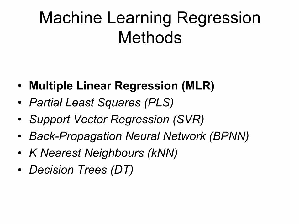
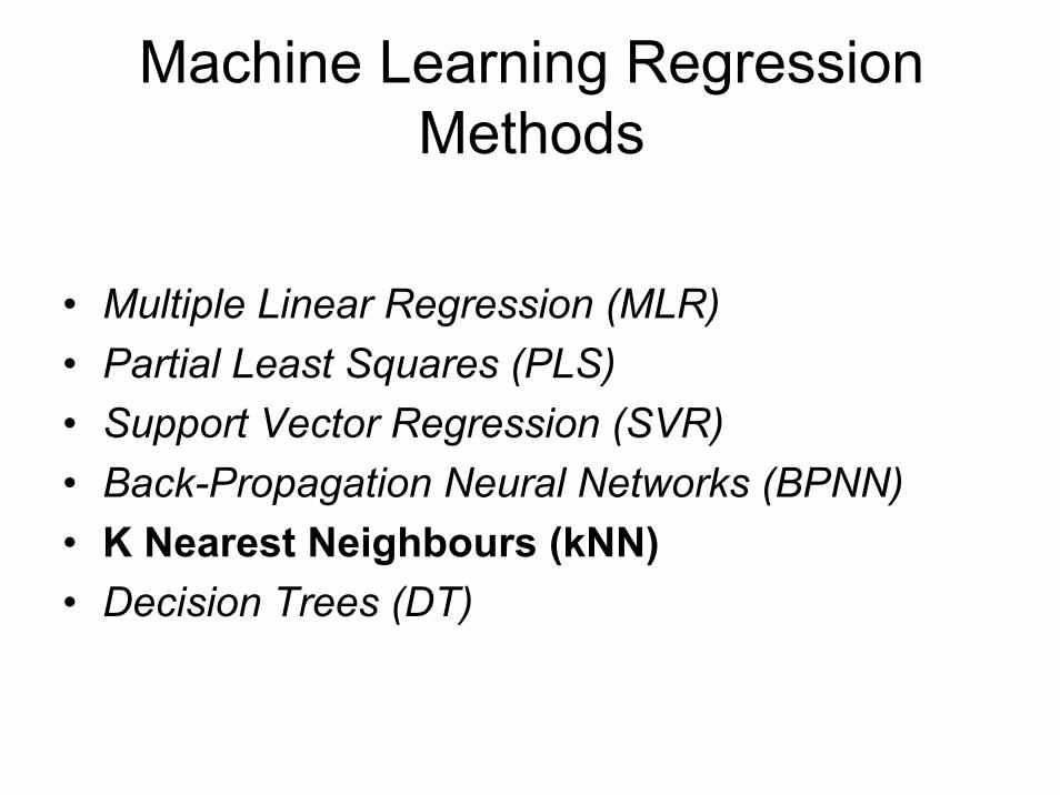
Machine Learning Regression Methods

• Multiple Linear Regression (MLR)• Partial Least Squares (PLS)• Support Vector Regression (SVR)• Back-Propagation Neural Network (BPNN)• K Nearest Neighbours (kNN)• Decision Trees (DT)

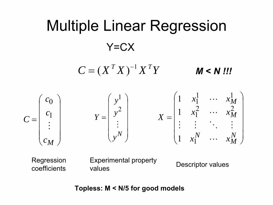
Multiple Linear Regression

YXXXC TT 1)( −=

⎟⎟⎟⎟⎟

⎠

⎞

⎜⎜⎜⎜⎜

⎝

⎛

=

Mc

cc

CM1

0

⎟⎟⎟⎟⎟

⎠

⎞

⎜⎜⎜⎜⎜

⎝

⎛

=

Ny

yy

YM

2

1

⎟⎟⎟⎟⎟

⎠

⎞

⎜⎜⎜⎜⎜

⎝

⎛

=

NM

N

M

M

xx

xxxx

X

L

MOMM

L

L

1

221

111

1

11

Regression coefficients

Experimental property values Descriptor values

M < N !!!

Topless: M < N/5 for good models

Y=CX

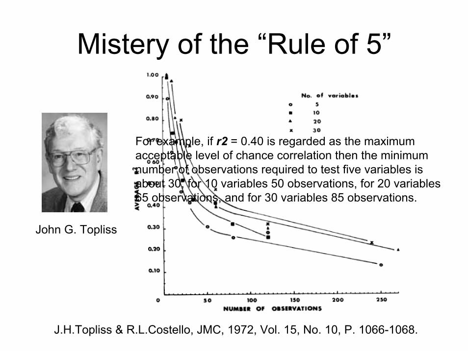
Mistery of the “Rule of 5”

John G. Topliss

J.H.Topliss & R.L.Costello, JMC, 1972, Vol. 15, No. 10, P. 1066-1068.

For example, if r2 = 0.40 is regarded as the maximumacceptable level of chance correlation then the minimumnumber of observations required to test five variables isabout 30, for 10 variables 50 observations, for 20 variables65 observations, and for 30 variables 85 observations.

Mistery of the “Rule of 5”C.Hansch, K.W.Kim, R.H.Sarma, JACS, 1973, Vol. 95, No.19, 6447-6449

Topliss and Costello2 have pointed out the danger of finding meaningless chance correlations with three or four data points per variable.

The correlation coefficient is good and there are almost five data pointsper variable.

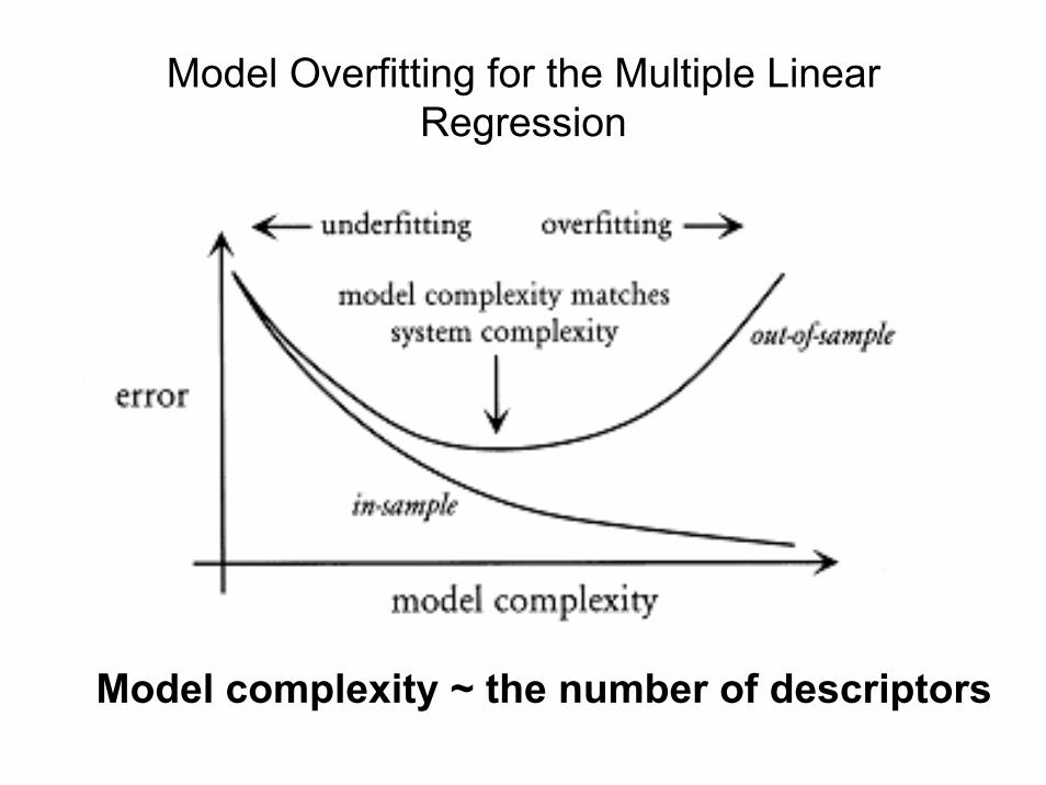
Model Overfitting for the Multiple Linear Regression

Model complexity ~ the number of descriptors

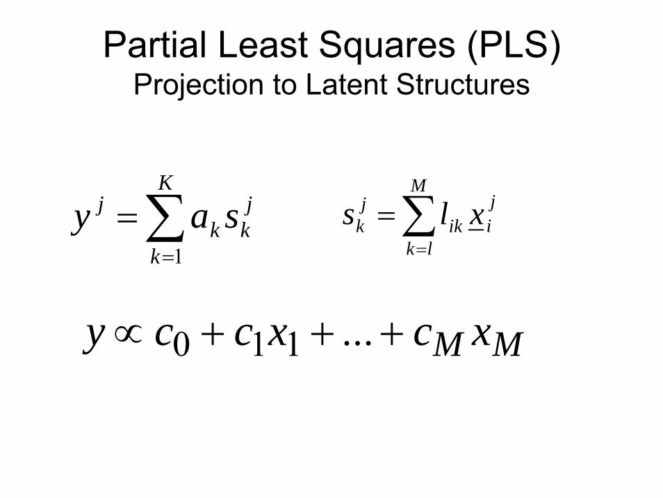
Partial Least Squares (PLS)Projection to Latent Structures

∑=

=K

k

jkk

j say1

∑=

=M

lk

jiik

jk xls

MM xcxccy +++∝ ...110

Principal Component Analysis (PCA)

⎪⎩

⎪⎨

⎧

=≠=

=

1),(,0),(

)}max{var(arg

ii

ki

Tii

llkill

Xll

rr

rr

rr

Partial Least Squares (PLS)

⎪⎩

⎪⎨

⎧

=≠=

=

1),(,0),(

)},max{cov(arg

ii

ki

Tii

llkill

Xlyl

rr

rr

rrr

Dependence of R2,Q2 upon the Number of Selected Latent Variables A

0

0.2

0.4

0.6

0.8

1

1.2

1 2 3 4 5 6 7 8 9 10A

R2,

Q2 R2

Q2

PLS (Aopt=5)

Q2(PLS)

MLR(A=rank(X))

Q2(MLR)

Herman Wold (1908-1992)

Swante Wold

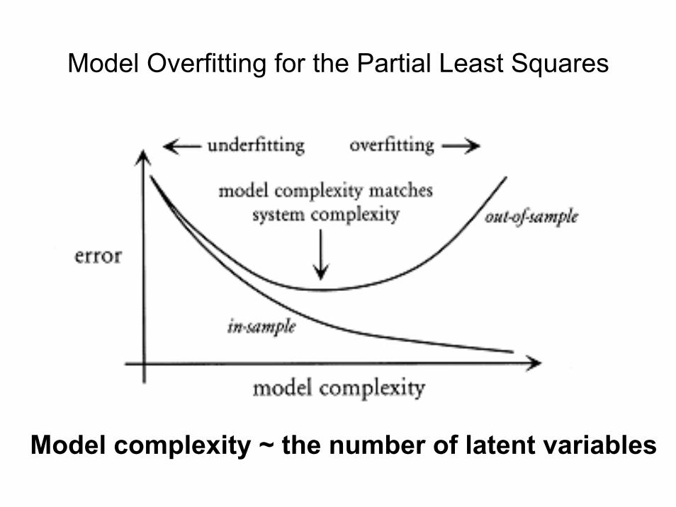
Model Overfitting for the Partial Least Squares

Model complexity ~ the number of latent variables

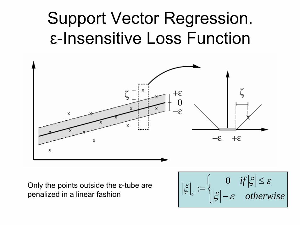
Support Vector Regression. ε-Insensitive Loss Function

⎩⎨⎧

−≤

=otherwise

ifεξ

εξξ

ε

0:Only the points outside the ε-tube are

penalized in a linear fashion

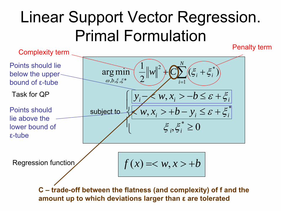
Linear Support Vector Regression. Primal Formulation

∑=

++N

iii

bCw

1

*2

*,,,)(

21minarg ξξ

ξξω

⎪⎩

⎪⎨

⎧

≥+≤−+><+≤−><−

0,,

,

*

*

ii

iii

iii

ybxwbxwy

ξξξεξε

subject to

Regression function bxwxf

Task for QP

+>=< ,)(

C – trade-off between the flatness (and complexity) of f and the amount up to which deviations larger than ε are tolerated

Complexity termPenalty term

Points should lie below the upper bound of ε-tube

Points should lie above the lower bound of ε-tube

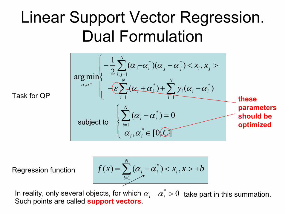
Linear Support Vector Regression. Dual Formulation

⎪⎪⎩

⎪⎪⎨

⎧

−++−

><−−−

∑ ∑

∑

= =

=N

i

N

iiiiii

N

jijijjii

y

xx

1 1

**

1,

**

*, )()(

,))((21

minargααααε

αααα

αα

⎪⎩

⎪⎨⎧

∈

=−∑=

],0[,

0)(*

1

*

Cii

N

iii

αα

ααsubject to

∑=

+><−=N

iiii bxxxf

1

* ,)()( αα

Task for QP

Regression function

these parameters should be optimized

In reality, only several objects, for which 0* >− ii ααSuch points are called support vectors.

take part in this summation.

Dualism of QSAR/QSPR Models

bxwxf +>=< ,)(Primal formulation

Dual formulation

Ordinary method

Similarity-based method

∑=

+><−=N

iiii bxxxf

1

* ,)()( αα

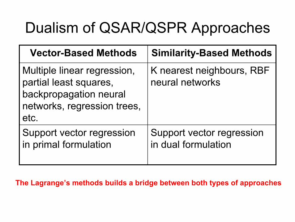
Dualism of QSAR/QSPR ApproachesVector-Based Methods Similarity-Based Methods

Multiple linear regression, partial least squares, backpropagation neural networks, regression trees, etc.

K nearest neighbours, RBF neural networks

Support vector regression in primal formulation

Support vector regression in dual formulation

The Lagrange’s methods builds a bridge between both types of approaches

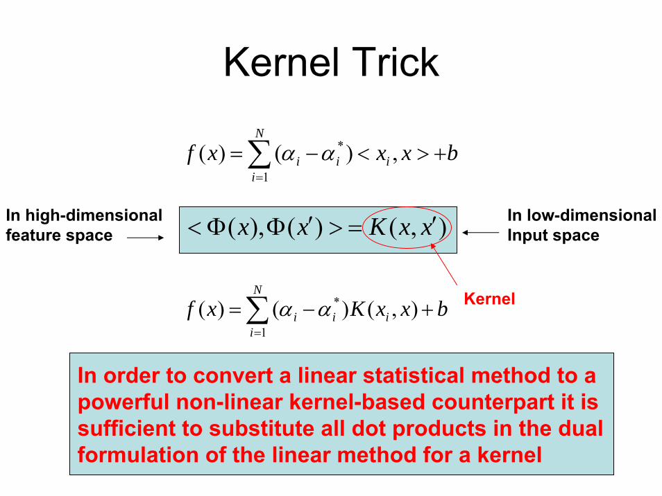
Kernel Trick

Any non-linear problem (classification, regression) in the original input space can be converted into linear by making non-linear mapping Φ into a feature space with higher dimension

Kernel Trick

∑=

+><−=N

iiii bxxxf

1

* ,)()( αα

In order to convert a linear statistical method to a powerful non-linear kernel-based counterpart it is sufficient to substitute all dot products in the dual formulation of the linear method for a kernel

),()(),( xxKxx ′=>′ΦΦ<

Kernel∑=

+−=N

iiii bxxKxf

1

* ),()()( αα

In high-dimensional feature space

In low-dimensionalInput space

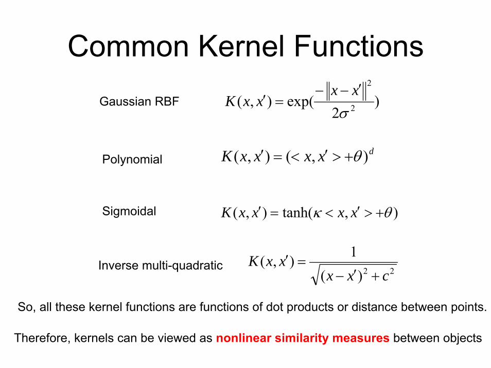
Common Kernel FunctionsGaussian RBF )

2exp(),( 2

2

σxx

xxK′−−

=′

PolynomialdxxxxK ),(),( θ+>′<=′

Sigmoidal ),tanh(),( θκ +>′<=′ xxxxK

Inverse multi-quadratic 22)(1),(

cxxxxK

+′−=′

So, all these kernel functions are functions of dot products or distance between points.

Therefore, kernels can be viewed as nonlinear similarity measures between objects

Function Approximation with SVR with Different Values of ε

ε=0.5 ε=0.2

ε=0.1 ε=0.02

line – regression function f(x)

small points – data points

big points – support vectors

So, the number of support vectors increases with the decrease of ε

Model Overfitting for the Support Vector Regression

Model complexity ~ 1/ε ~ the number of support vectors

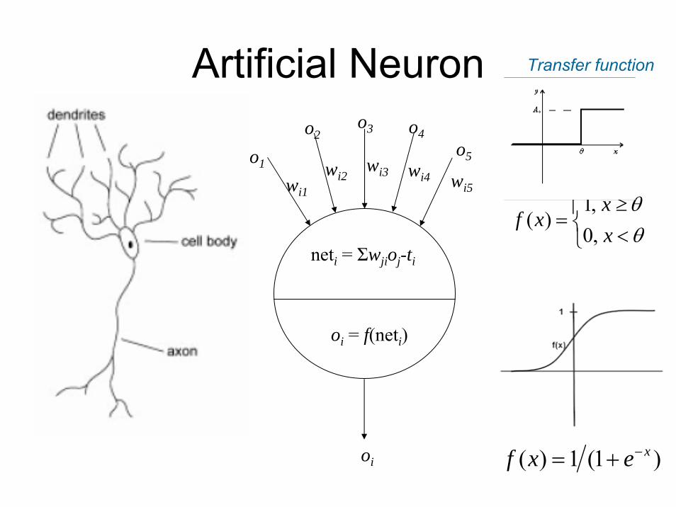
Artificial Neuron

wi5wi4

wi3wi2wi1

o5

o3 o4

o1

O2O2o2

oi = f(neti)

oi

neti = Σwjioj-ti

)1(1)( xexf −+=

⎩⎨⎧

<≥

=θθ

xx

xf,0,1

)(

Transfer function

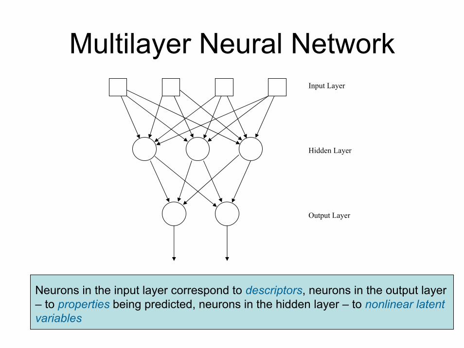
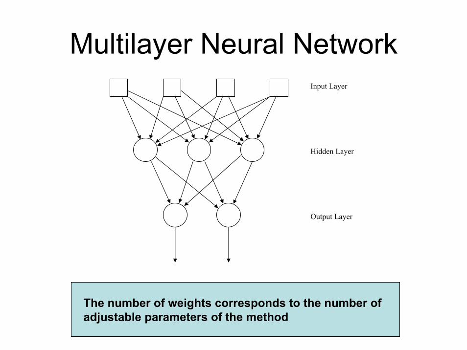
Multilayer Neural NetworkInput Layer

Hidden Layer

Output Layer

Neurons in the input layer correspond to descriptors, neurons in the output layer – to properties being predicted, neurons in the hidden layer – to nonlinear latent variables

Generalized Delta-RuleThis is application of the steepest descent method to training backpropagation neural networks

')(ji

jji

ij

empij y

deedf

yw

Rw δηδηη −=−=

∂

∂−=Δ

η – learning rate constant

1974

Paul WerbosDavid

RummelhardJames

McClelland

1986

Geoffrey Hinton

Multilayer Neural NetworkInput Layer

Hidden Layer

Output Layer

The number of weights corresponds to the number of adjustable parameters of the method

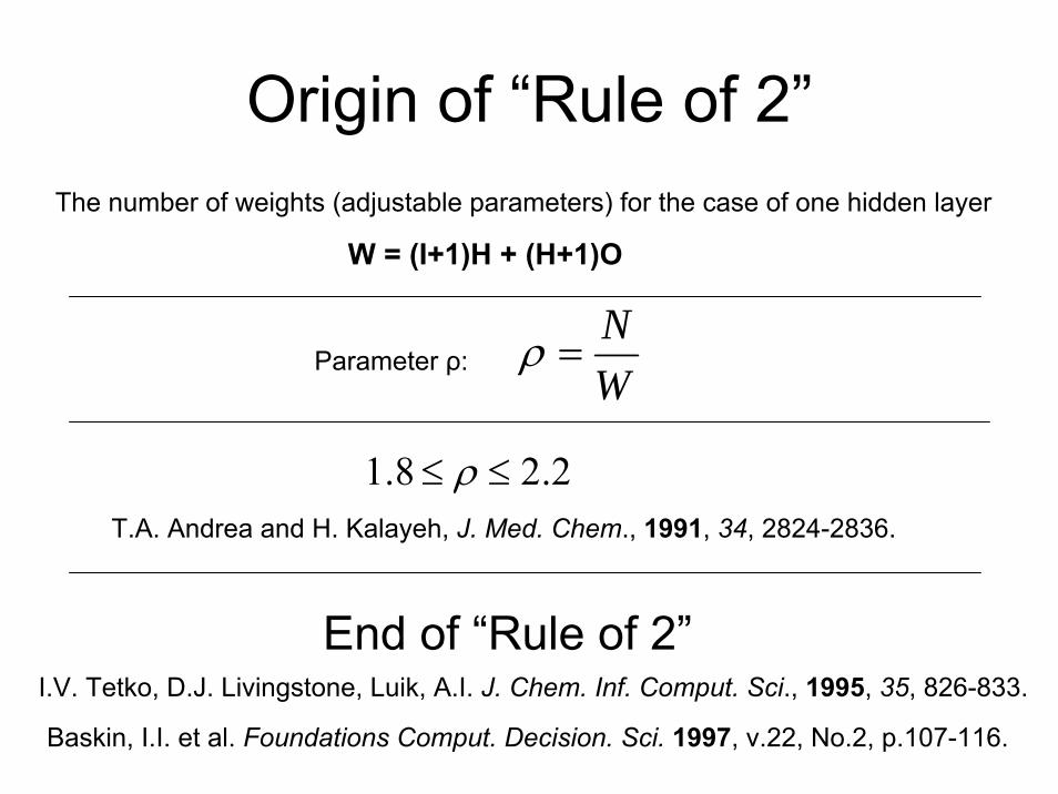
Origin of “Rule of 2”The number of weights (adjustable parameters) for the case of one hidden layer

W = (I+1)H + (H+1)O

2.28.1 ≤≤ ρT.A. Andrea and H. Kalayeh, J. Med. Chem., 1991, 34, 2824-2836.

Parameter ρ:WN

=ρ

End of “Rule of 2”I.V. Tetko, D.J. Livingstone, Luik, A.I. J. Chem. Inf. Comput. Sci., 1995, 35, 826-833.

Baskin, I.I. et al. Foundations Comput. Decision. Sci. 1997, v.22, No.2, p.107-116.

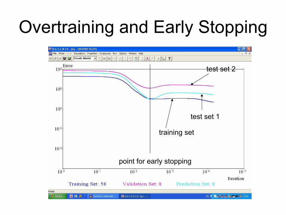
Overtraining and Early Stopping

training set

test set 1

test set 2

point for early stopping

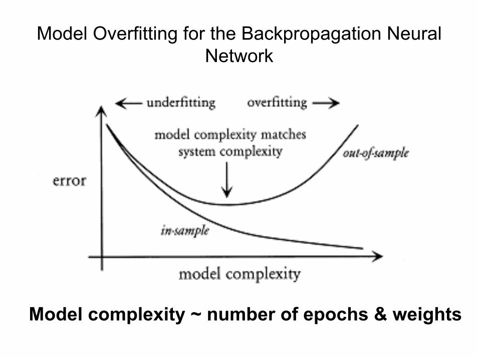
Model Overfitting for the Backpropagation Neural Network

Model complexity ~ number of epochs & weights


• Multiple Linear Regression (MLR)• Partial Least Squares (PLS)• Support Vector Regression (SVR)• Back-Propagation Neural Networks (BPNN)• K Nearest Neighbours (kNN)• Decision Trees (DT)

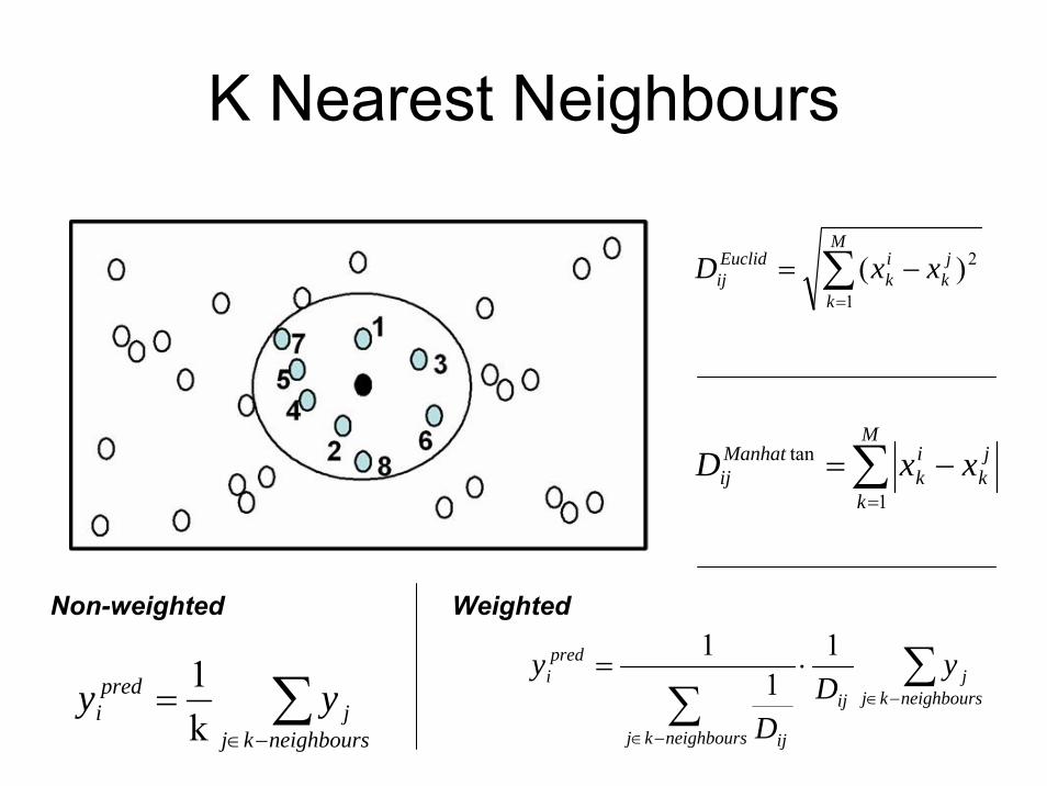
K Nearest Neighbours

∑=

−=M

k

jk

ik

Euclidij xxD

1

2)(

∑=

−=M

k

jk

ik

Manhatij xxD

1

tan

∑−∈

=neighbourskj

jpredi yy

k1 ∑

∑ −∈

−∈

⋅=neighbourskj

jij

neighbourskj ij

predi y

DD

y 11

1Non-weighted Weighted

Overfitting by Variable Selection in kNN

Golbraikh A., Tropsha A. Beware of q2! JMGM, 2002, 20, 269-276

Model Overfitting for the k Nearest Neighbours

Model complexity ~ selection of descriptors ~1/k


• Multiple Linear Regression (MLR)• Partial Least Squares (PLS)• Support Vector Regression (SVR)• Back-Propagation Neural Networks (BPNN)• K Nearest Neighbours (kNN)• Decision Trees (DT)

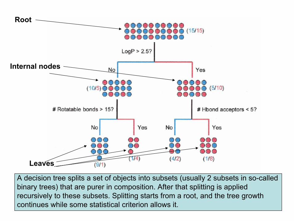
A decision tree splits a set of objects into subsets (usually 2 subsets in so-called binary trees) that are purer in composition. After that splitting is applied recursively to these subsets. Splitting starts from a root, and the tree growth continues while some statistical criterion allows it.

Root

Leaves

Internal nodes

Overfitting and Early Stopping of Tree Growth

Decision trees can overfit data. So, it is necessary to use an external test set in order to stop tree growth at the optimal tree size

Stop learning here

Decision Tree for Biodegradability

- biodedagrable

- nonbiodedagrable

JCICS, 2004, 44, 862-870

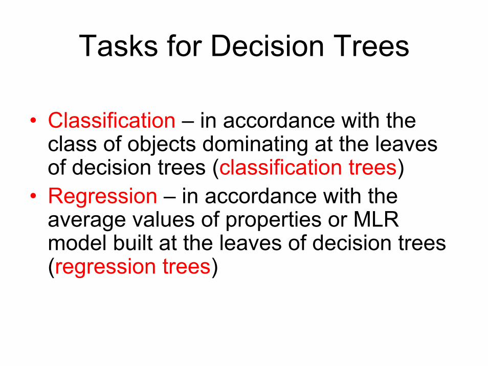
Tasks for Decision Trees

• Classification – in accordance with the class of objects dominating at the leaves of decision trees (classification trees)

• Regression – in accordance with the average values of properties or MLR model built at the leaves of decision trees (regression trees)

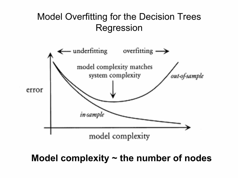
Model Overfitting for the Decision Trees Regression

Model complexity ~ the number of nodes

Conclusions

• There are many machine learning methods

• Different problems may require different methods

• All methods could be prone of overfitting• But all of them have facilities to tackle this

problem

Exam. Question 1

What is it?

1. Support Vector Regression

2. Backpropagation Neural Network

3. Partial Least Squares Regression

Exam. Question 2Which method is not prone to overfitting?

1. Multiple Linear Regression2. Partial Least Squares3. Support Vector Regression4. Backpropagation Neural Networks5. K Nearest Neighbours6. Decision Trees7. Neither

modern machine learning methods - home - laboratoire...

Documents