modelling with auto_cad_2002
TRANSCRIPT

Modelling with AutoCAD 2002
modelling with AutoCAD.qxd 17/06/2002 15:37 Page i

Other titles from Bob McFarlane
Beginning AutoCAD ISBN 0 340 58571 4
Progressing with AutoCAD ISBN 0 340 60173 6
Introducing 3D AutoCAD ISBN 0 340 61456 0
Solid Modelling with AutoCAD ISBN 0 340 63204 6
Assignments in AutoCAD ISBN 0 340 69181 6
Starting with AutoCAD LT ISBN 0 340 62543 0
Advancing with AutoCAD LT ISBN 0 340 64579 2
3D Draughting using AutoCAD ISBN 0 340 67782 1
Beginning AutoCAD R13 for Windows ISBN 0 340 64572 5
Advancing with AutoCAD R13 for Windows ISBN 0 340 69187 5
Modelling with AutoCAD R13 for Windows ISBN 0 340 69251 0
Using AutoLISP with AutoCAD ISBN 0 340 72016 6
Beginning AutoCAD R14 for Windows NT and Windows 95 ISBN 0 340 72017 4
Advancing with AutoCAD R14 for Windows NT and Windows 95 ISBN 0 340 74053 1
Modelling with AutoCAD R14 for Windows NT and Windows 95 ISBN 0 340 73161 3
An Introduction to AEC 5.1 with AutoCAD R14 ISBN 0 340 74185 6
modelling with AutoCAD.qxd 17/06/2002 15:37 Page ii

Modelling withAutoCAD 2002Bob McFarlaneMSc, BSc, ARCSTCEng, FIED, RCADDesMIMechE, MIEE, MIMgt, MBCS, MCSD
Curriculum Manager CAD and New Media, Motherwell College,Autodesk Educational Developer
OXFORD AMSTERDAM BOSTON LONDON NEW YORK PARISSAN DIEGO SAN FRANCISCO SINGAPORE SYDNEY TOKYO
modelling with AutoCAD.qxd 17/06/2002 15:37 Page iii

Butterworth-Heinemann An imprint of Elsevier Science Linacre House, Jordan Hill, Oxford OX2 8DP225 Wildwood Avenue, Woburn, MA 01801-2041
First published 2002
Copyright © 2002, R. McFarlane. All rights reserved
The right of Bob McFarlane to be identified as the author of this work has been asserted in accordance with the Copyright, Designs and Patents Act 1988.
No part of this publication may be reproduced in any material form (including photocopying or storing in any medium by electronic means and whether or not transiently or incidentally to some other use of this publication) without the written permission of the copyright holder except in accordance with the provisions of the Copyright, Designs and Patents Act 1988 or under the terms of a licence issued by the Copyright Licensing Agency Ltd, 90 Tottenham Court Road, London, England W1T 4LP. Applications for the copyright holder’s written permission to reproduce any part of this publication should be addressed to the publisher
British Library Cataloguing in Publication DataA catalogue record for this book is available from the British Library
Library of Congress Cataloguing in Publication DataA catalogue record for this book is available from the Library of Congress
ISBN 0 7506 5611 5
Produced and typeset by Gray Publishing, Tunbridge Wells, KentPrinted and bound in Great Britain by Bath Press, Avon
For information on all Butterworth-Heinemannpublications visit our website at www.bh.com
modelling with AutoCAD.qxd 17/06/2002 15:37 Page iv
ContentsPreface vii
Chapter 1 The 3D standard sheet 1
Chapter 2 Extruded 3D models 5
Chapter 3 The UCS and 3D coordinates 14
Chapter 4 Creating a 3D wire-frame model 24
Chapter 5 The UCS 32
Chapter 6 The modify commands with 3D models 44
Chapter 7 Dimensioning in 3D 47
Chapter 8 Hatching in 3D 52
Chapter 9 Tiled viewports 56
Chapter 10 3D views (Viewpoint) 64
Chapter 11 Model space and paper space and untiled viewports 83
Chapter 12 New 3D multiple viewport standard sheet 91
Chapter 13 Surface modelling 100
Chapter 14 3DFACE and PFACE 110
Chapter 15 3DMESH 110
Chapter 16 Ruled surface 113
Chapter 17 Tabulated surface 121
Chapter 18 Revolved surface 123
Chapter 19 Edge surface 127
Chapter 20 3D polyline 133
Chapter 21 3D objects 136
Chapter 22 3D geometry commands 139
Chapter 23 Blocks and Wblocks in 3D 151
Chapter 24 Dynamic viewing 161
modelling with AutoCAD.qxd 17/06/2002 15:37 Page v

Chapter 25 Viewport specific layers 169
Chapter 26 Shading and 3D orbit 173
Chapter 27 Introduction to solid modelling 179
Chapter 28 The basic solid primitives 184
Chapter 29 The swept solid primitives 196
Chapter 30 Boolean operations and composite solids 205
Chapter 31 Composite model 1 – a machine support 209
Chapter 32 Composite model 2 – a backing plate 214
Chapter 33 Composite model 3 – a flange and pipe 219
Chapter 34 The edge primitives 222
Chapter 35 Solids editing 228
Chapter 36 Regions 235
Chapter 37 Inquiring into solids 241
Chapter 38 Slicing and sectioning solid models 247
Chapter 39 Profiles and true shapes 255
Chapter 40 Dimensioning in model and paper space 262
Chapter 41 A detailed drawing 267
Chapter 42 Blocks, wblocks and external references 273
Chapter 43 The setup commands 286
Chapter 44 The final composite 295
Chapter 45 Rendering 302
Chapter 46 Publishing to the web 312
Chapter 47 Students’ models 316
Activities 323
Index 335
vi Modelling with AutoCAD 2002
modelling with AutoCAD.qxd 17/06/2002 15:37 Page vi

PrefaceThis book is intended for the AutoCAD 2002 user who wants to learn about modelling.My aim is to demonstrate how the user can create 3D wire-frame models, surface modelsand solid models with practical exercises backed up by user activities. The concept ofhow multiple viewports can be used to enhance drawing productivity will also bediscussed in detail. The user will also be introduced to rendering.
The book will provide an invaluable aid to a wide variety of users, ranging from thecapable to the competent. The book will assist students on any national course whichrequires 3D draughting and solid modelling, e.g. City and Guilds, BTEC and SQA as wellas students at higher institutions. Users in industry will find the book useful as areference and an ‘inspiration’. The book will also prove useful to the Design/Technologydepartments in schools who are now becoming more involved in computer aided design.
Reader requirementsThe following are the requirements I consider important for using the book:a) the ability to draw with AutoCAD 2002b) the ability to use icons and toolbarsc) an understanding of how to use dialogue boxesd) the ability to open and save drawings to a named foldere) a knowledge of model/paper space would be an advantage, although this is not
essential
Using the bookThe book is essentially a self-teaching package with the reader working interactivelythrough exercises using information supplied. The various prompts and responses willbe listed in order and icons and dialogue boxes will be included where appropriate.
The following points are important:a) All drawing work should be saved to a named folder. The folder name is at your
discretion but I will refer to it as MODR2002, e.g. open drawingMODR2002\MODEL1 or similar
b) Icons will be displayed the first time is usedc) Menu bar selection will be in bold type, e.g. Draw-Surfaces-3D Faced) Keyboard entry will also be in bold type, e.g. VPOINT, UCS etce) Prompts will be in typewrite type, e.g. First cornerf) The symbol <R> will require the user to press the return/enter key.
NoteAll the exercises and activities have been completed using AutoCAD 2002. I have triedto correct any errors in the drawings and text, but if any error should occur, I apologisefor them and hope they do not spoil your learning experience. Modelling is an intriguingtopic and should give you satisfaction and enjoyment.
Any comments you have about how to improve the material in the book would be greatlyappreciated.
modelling with AutoCAD.qxd 17/06/2002 15:37 Page vii

To CIARA, our beautiful grand-daughter
modelling with AutoCAD.qxd 17/06/2002 15:37 Page viii
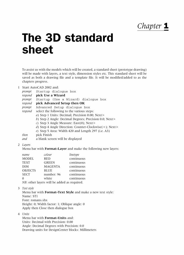
The 3D standardsheetTo assist us with the models which will be created, a standard sheet (prototype drawing)will be made with layers, a text style, dimension styles etc. This standard sheet will besaved as both a drawing file and a template file. It will be modified/added to as thechapters progress.
1 Start AutoCAD 2002 and:prompt Startup dialogue boxrespond pick Use a Wizardprompt Startup (Use a Wizard) dialogue boxrespond pick Advanced Setup then OKprompt Advanced Setup dialogue boxrespond select the following to the various steps:
a) Step 1 Units: Decimal; Precision 0.00; Next>b) Step 2 Angle: Decimal Degrees; Precision 0.0; Next>c) Step 3 Angle Measure: East(0); Next>d) Step 4 Angle Direction: Counter-Clockwise(+); Next>e) Step 5 Area: Width 420 and Length 297 (i.e. A3)
then pick Finishand a blank screen will be displayed
2 LayersMenu bar with Format-Layer and make the following new layers:
name colour linetypeMODEL RED continuousTEXT GREEN continuousDIM MAGENTA continuousOBJECTS BLUE continuousSECT number: 96 continuous0 white continuousNB: other layers will be added as required.
3 Text styleMenu bar with Format-Text Style and make a new text style:Name: ST1Font: romans.shxHeight: 0; Width factor: 1; Oblique angle: 0Apply then Close then dialogue box
4 UnitsMenu bar with Format-Units and:Units: Decimal with Precision: 0.00Angle: Decimal Degrees with Precision: 0.0Drawing units for DesignCenter blocks: Millimeters
Chapter 1
modelling with AutoCAD.qxd 17/06/2002 15:37 Page 1

5 LimitsMenu bar with Format-Drawing Limits and:prompt Specify lower left corner and enter: 0,0 <R>prompt Specify upper right corner and enter: 420,297 <R>
6 Drafting SettingsMenu bar with Tools-Drafting Settings and use the tabs to set:a) Snap: 5 and grid: 10 – not generally used in 3Db) Polar Tracking: offc) Object Snap: off and all modes: clear
Object Snap Tracking: off
7 Dimension styleMenu bar with Dimension-Style and:prompt Dimension Style Manager dialogue boxrespond pick Newprompt Create New Dimension Style dialogue boxrespond 1. New Style Name: 3DSTD
2. Start With: ISO-25 (or similar)3. Use for: All dimensions4. pick Continue
prompt New Dimension Style: 3DSTD dialogue boxrespond pick Lines and Arrows tab and alter:
1. Dimension Linesa) Baseline spacing: 10
2. Extension Linesa) Extend beyond dim lines: 2.5b) Offset from origin: 2.5
3. Arrowheadsa) both Closed Filledb) Leader: Closed Filledc) Arrow size: 4d) Center Mark for Circles: None
then pick Text tab and alter:1. Text Appearance
a) Text Style: ST1b) Text Height: 5
2. Text Placementa) Vertical: Aboveb) Horizontal: Centredc) Offset from dim line: 1.5
3. Text Alignmenta) ISO Standard
then pick Fit tab and alter:1. Fit Options
a) Either the text or the arrows active (black dot)2. Text Placement
a) Beside the dimension line active3. Scale for Dimension Features
a) Use overall scale of: 14. Fine tuning: both inactive, i.e. blank
2 Modelling with AutoCAD 2002
modelling with AutoCAD.qxd 17/06/2002 15:37 Page 2

then pick Primary Units tab and alter:1. Linear Dimensions
a) Unit Format: Decimalb) Precision: 0.00c) Decimal separator: ‘.’ Periodd) Round off: 0
2. Measurement Scalea) Scale factor: 1
3. Zero Suppressiona) Trailing: active, i.e. tick
4. Angular Dimensionsa) Units Format: Decimal Degreesb) Precision: 0.0c) Zero Suppression: Trailing active
then pick Alternate Units tab and:1. Display alternate units: not active
then pick Tolerances tab and:1. Tolerance Format
1 Method: Nonethen pick OK from New Dimension Style dialogue boxprompt Dimension Style Manager dialogue boxwith 1. 3DSTD added to styles list
2. preview of 3DSTD style displayed3. description of 3DSTD given
respond 1. pick 3DSTD and it becomes highlighted2. pick Set Current3. AutoCAD alert perhaps – just pick OK4. pick Close
8 Make layer 0 current and menu bar with Draw-Rectangle and:prompt Specify first corner point and enter: 0,0 <R>prompt Specify other corner point and enter: 420,290 <R>
9 This rectangle will save as a ‘reference base’ for our models
10 Menu bar with View-Zoom-All and pan to suit
11 Make layer MODEL current
12 Set variables to your own requirements, e.g. GRIPS, PICKFIRST, etc. While I generallywork with these off, there will be occasions when they will be toggled on
13 Menu bar with File-Save As and:prompt Save Drawing As dialogue boxrespond 1. scroll and pick named folder (MODR2002)
2. enter File name: 3DSTDA33. file type: AutoCAD 2000 Drawing (*.dwg)4. pick Save
The 3D standard sheet 3
modelling with AutoCAD.qxd 17/06/2002 15:37 Page 3

14 Menu bar with File-Save As and:prompt Save Drawing As dialogue boxrespond 1. scroll at Files of type
2. pick AutoCAD Drawing Template File (*.dwt)3. scroll and pick named folder4. enter File name as: 3DSTDA35. pick Save
prompt Template Description dialogue boxrespond 1. Enter: This is my 3D standard sheet
2. pick OK
15 The created standard sheet has been saved as a drawing file and a template file, bothwith the name 3DSTDA3. Both have been saved to the MODR2002 named folder – orthe name you have given the folder to save all modelling work.
16 Notea) we could have saved the template file to the AutoCAD Template file – you still can if
you wantb) saving the standard sheet as a template will stop the user ‘inadvertently’ over-writing
the basic 3DSTD standard drawing sheetc) all models will be created from the 3DSTDA3 template filed) all completed models will be saved as drawings to your named foldere) the standard sheet has been saved as a drawing file as backup
We are now ready to proceed with creating 3D and solid models.
4 Modelling with AutoCAD 2002
modelling with AutoCAD.qxd 17/06/2002 15:37 Page 4

Extruded 3D modelsAn extruded model is created by extruding a ‘shape’ upwards or downwards from ahorizontal plane – called the ELEVATION plane. The actual extruded height (or depth)is called the THICKNESS and can be positive or negative relative to the set elevationplane. This extruded thickness is always perpendicular to the elevation plane. Theextrusion is in the Z direction of the UCS icon – more on the UCS later. The basicextruded terminology is displayed in Fig. 2.1.
Note: Extruded models were one of the first ever 3D displays with a CAD system. Theterm 3D model is not quite correct, a more accurate description being 21/2D model.
Chapter 2
Figure 2.1 Basic extruded terminology.
modelling with AutoCAD.qxd 17/06/2002 15:37 Page 5

Example 1The example is given as a series of user entered steps, these steps also being displayedin Fig. 2.2. The exercise will introduce the user to some of the basic 3D commands andconcepts.
To get started:
1 Open your 3DSTDA3 template file and display toolbars to suit e.g. Draw, Modify and Object Snap.
2 Layer MODEL should be current.
Step 1: the first elevation1. At the command line enter ELEV <R> and:
prompt Specify new default elevation<0.00> and enter: 0 <R>prompt Specify new default thickness<0.00> and enter: 50 <R>
2. Nothing appears to have happened?3. Select the LINE icon and draw:
Start point: 40,40 <R>Next point: @100,0 <R>Next point: @100<90 <R>Next point: @–100,0 <R>Next point: C <R> – the close option
4. A red ‘square’ will be displayed.
6 Modelling with AutoCAD 2002
Figure 2.2 Extruded example 1.
modelling with AutoCAD.qxd 17/06/2002 15:37 Page 6

Step 2: the second elevation1. At the command line enter ELEV <R> and:
prompt Specify new default elevation<0.00> and enter: 50 <R>prompt Specify new default thickness<50.00> and enter: 30 <R>
2. Select the CIRCLE icon and:a) centre point: enter 90,90 <R>b) radius: enter 40 <R>
3. At the command line enter CHANGE <R> and:prompt Select objectsrespond pick the circle then right-clickprompt Specify change point or [Properties]enter P <R> – the properties optionprompt Enter property to change [Color/Elev/Layer/Ltype etcenter C <R> – the color optionprompt Enter new colorenter green <R>prompt Enter property to changerespond right-click and pick Enter
4. The added circle will be displayed with a green colour
Step 3: the third elevation1. With the ELEV command:
a) set the default elevation to 80b) set the default thickness to 10
2. With the LINE icon, draw:Start point: 70,70 <R>Next point: 110,70 <R>Next point: 90,120 <R>Next point: C <R>
3. With the CHANGE command, change the colour of the three lines to blue, using thesame procedure as was used previously.
4. We now have a blue triangle inside a green circle inside a red square, and appear tohave a traditional 2D plan type drawing.
5. Each of the three shapes has been created on a different default elevation plane:a) square: elevation 0b) circle: elevation 50c) triangle: elevation 80
Step 4: viewing the model in 3DTo ‘see’ the model in 3D the 3D Viewpoint command is required, so:1. From the menu bar select View-3D Views-SE Isometric2. The model will be displayed in 3D. The black ‘drawing border’ is also displayed in 3D
and acts as a ‘base’ for the model.3. The orientation of the model is such that it is difficult to know if you are looking down
on it, or looking up at it. This is common with 3D modelling and is calledAMBIGUITY. Another command is required to ‘remove’ this ambiguity.
4. At this stage save your model with File-Save As and ensure:a) File type is: AutoCAD 2000 Drawing (*.dwg)b) Save in: MODR2002 – your named folderc) File name: EXT-1 – the drawing name
5. This saves the drawing as C:\MODR2002\EXT-1.dwg – the path name
Extruded 3D models 7
modelling with AutoCAD.qxd 17/06/2002 15:37 Page 7

Step 5: the hide command1. From the menu bar select View-Hide and the model will be displayed with hidden
line removal. It is now easier to visualise.2. From the screen display it is obvious that the model is being viewed from above, but
it is possible to view from different angles.3. Menu bar with View-Regen to ‘restore’ the original model
Step 6: another viewpoint1. At the command line enter VPOINT <R> and:
prompt Specify a view point or [Rotate]enter R <R> – the rotate optionprompt Enter angle in XY plane from X-axis and enter: 315 <R>prompt Enter angle in XY plane and enter: –10 <R>
2. The model will be displayed from a different viewpoint without hidden line removal3. At the command line enter HIDE <R>4. The model will be displayed with hidden line removal and is being viewed from below5. At the command line enter REGEN <R> to restore the original
Step 7: the shade command1. Restore the original 3D view with the menu bar sequence View-3D Views-SE
Isometric2. Menu bar with View-Shade-Flat Shaded and the model will be displayed in colour.
This is the result of the change command after the various objects had been drawn.3. Note the icon – more on this later4. Menu bar with View-Shade-Gouraud Shaded and note the effect on the model.
Can you observe any difference between the flat shading and the Gouraud shading?Look at the ‘cylinder’ part of the model
5. Investigate the other SHADE options available6. Restore the model to its original display with View-Shade-2D Wireframe and note
the icon.
Task1 With the ERASE command pick any line of the ‘base’ and a complete ‘side’ is erased
because it is an extrusion
2 Undo the erase effect with U <R>
3 Using the erase command pick any point on the top ‘circle’ and the complete ‘cylinder’will be erased.
4 Undo this erase effect.
5 This completes our first extrusion exercise.
6 Note:Although Fig. 2.2 displays several different viewpoints of the model on ‘one sheet’ thisconcept will not be discussed until a later chapter. At present you will only display asingle viewpoint of the model.
8 Modelling with AutoCAD 2002
modelling with AutoCAD.qxd 17/06/2002 15:37 Page 8
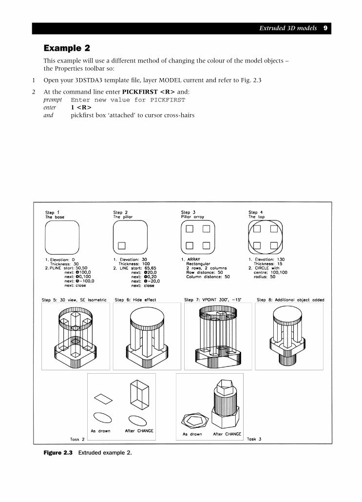
Example 2This example will use a different method of changing the colour of the model objects –the Properties toolbar so:
1 Open your 3DSTDA3 template file, layer MODEL current and refer to Fig. 2.3
2 At the command line enter PICKFIRST <R> and:prompt Enter new value for PICKFIRSTenter 1 <R>and pickfirst box ‘attached’ to cursor cross-hairs
Extruded 3D models 9
Figure 2.3 Extruded example 2.
modelling with AutoCAD.qxd 17/06/2002 15:37 Page 9

Step 1: the base1. With ELEV at the command line, set the new default elevation to 0 and the new
default thickness to 302. With the polyline icon from the Draw toolbar, draw a 0 width polyline:
Start point 50,50 <R>Next point @100,0 <R>Next point @0,100 <R>Next point @–100,0 <R>Next point C <R>
3. Menu bar with Modify-Fillet and:prompt Select first object or [Polyline/Radius/Trim]enter R <R> – the radius optionprompt Specify fillet radiusenter 20 <R>prompt Select first object [Polyline/Radius/Trim]enter P <R> – polyline optionprompt Select 2D polylinerespond pick any point on the polyline
4. The red polyline will be filleted at the four cornersStep 2: the first pillar1. Set the elevation to 30 and the thickness to 1002. With the LINE command, draw a 20 unit square the lower left corner being at the
point 65,653. Using the pickbox on the cursor, pick the four lines of the square then select the
Properties icon from the Standard toolbar and:prompt Properties dialogue boxrespond 1. pick Categorised tab
2. pick Color line – highlights3. scroll at right of Color line4. pick Blue – Fig. 2.45. Close the Properties dialogue box – top right pick6. press ESC key
4. The square will be displayed with blue lines
10 Modelling with AutoCAD 2002
Figure 2.4 The Properties dialogue box for the selected square.
modelling with AutoCAD.qxd 17/06/2002 15:37 Page 10

Step 3: arraying the pillar1. Select the ARRAY icon from the Modify toolbar and:
prompt Array dialogue boxrespond 1. Rectangular Array active
2. Rows: 2; Columns: 23. Row offset: 50 and Column offset: 504. Angle of Array: 05. pick Select objects and:
prompt Select objects at the command linerespond window the blue square then right-clickprompt Array dialogue boxrespond pick Preview<and blue square arrayed as expected? then Array message and pick Accept
2. The blue square will be arrayed in a 2×2 matrix pattern
Step 4: the top1. Set the elevation to 130 and the thickness to 152. Draw a circle, centred on 100,100 with radius of 503. Using the pickbox:
a) pick the circle then the Properties iconb) set the colour to green
Step 5: the 3D viewpoint1. Menu bar with View-3D Views-SE Isometric2. The model is displayed in 3D but appears rather ‘cluttered’
Step 6: hiding the model1. Menu bar with View-Hide model displayed with hidden line removal2. Menu bar with View-Regen to restore the original model
Step 7: setting another viewpoint1. At the command line enter VPOINT <R> and:
prompt Specify a new view point or [Rotate]enter R <R> – the rotate optionprompt Enter angle in XY plane from X axis and enter: 300 <R>prompt Enter angle from XY plane and enter: –15 <R>
2. Menu bar with View-Hide to ‘see’ the model from below 3. Menu bar with View-Regen to restore the original model4. Restore the original 3D view with View-3D Views-SE Isometric
Step 81. The model should be displayed in 3D at a SE Isometric viewpoint2. Using the command line, set the elevation to 0 and the thickness to –603. Draw a circle with centre at 100,100 and radius 304. The circle will be displayed in 3D as a ‘cylinder’5. Change the colour of the added ‘cylinder’ to magenta6. As the model is complete, save as C:\MODR2002\EXT-2
Extruded 3D models 11
modelling with AutoCAD.qxd 17/06/2002 15:37 Page 11

Task 1Use the menu bar with the following menu bar sequences:a) View-3D Views-SE Isometricb) View-Hide and note green circle displayc) View-Shade-Flat Shaded and note colour effect and icond) View-Shade-3D Wireframee) View-Hide and note the green circle displayf) View-Shade-Flat Shaded, Edges Ong) View-Shade-2D Wireframe and note the green circle displayh) View-Regen to ‘restore’ the original model
Task 21 Still with the SE Isometric viewpoint displayed
2 Set the elevation to 0 and the thickness to 100
3 With Draw-Rectangle create a rectangle anywhere on the screen
4 With Draw-Ellipse-Center create an ellipse anywhere on the screen
5 Both the rectangle and the ellipse will be drawn without any thickness, although thethickness was set to 100 in step 2
6 At the command line enter CHANGE <R> and:prompt Select objectsrespond pick any point on the rectangle then right-clickprompt Specify change point or [Properties]enter P <R> – the Properties optionprompt Enter property to change [Color/Elev/Layer etcenter T <R> – the thickness optionprompt Specify new thickness <0.00>enter 100 <R>prompt Enter property to changeenter <R> – to end command as no other properties to change
7 The rectangle will now be displayed in 3D with a thickness
8 Using the same sequence and entries as step 6, select the ellipse. No thickness will ‘be added’
9 With the CHANGE command, alter the elevation of the ellipse to 50.
Task 31 Display a SE Isometric viewpoint and set the elevation and thickness both to 0. Layer
MODEL still current
2 Draw the following objects:a) polygon with 6 sides, centred on 0,0 and inscribed in a 50 radius circleb) circle, centre on 0,0 with radius 40c) polygon with 5 sides, centred on 0,0 and inscribed in a 30 radius circle
3 Set PICKFIRST to 0 then use the CHANGE command to alter the three objects with thefollowing information:
object elev thickness colour6 sided polygon 0 50 redcircle 50 80 blue5 sided polygon 130 30 green
4 Investigate the hide and shade commands and other 3D viewpoints
5 This exercise is now complete. Do not save these additions.
12 Modelling with AutoCAD 2002
modelling with AutoCAD.qxd 17/06/2002 15:37 Page 12
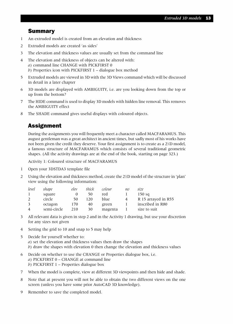
Summary1 An extruded model is created from an elevation and thickness
2 Extruded models are created ‘as sides’
3 The elevation and thickness values are usually set from the command line
4 The elevation and thickness of objects can be altered with:a) command line CHANGE with PICKFIRST 0b) Properties icon with PICKFIRST 1 – dialogue box method
5 Extruded models are viewed in 3D with the 3D Views command which will be discussedin detail in a later chapter
6 3D models are displayed with AMBIGUITY, i.e. are you looking down from the top orup from the bottom?
7 The HIDE command is used to display 3D models with hidden line removal. This removesthe AMBIGUITY effect
8 The SHADE command gives useful displays with coloured objects.
AssignmentDuring the assignments you will frequently meet a character called MACFARAMUS. Thisaugust gentleman was a great architect in ancient times, but sadly most of his works havenot been given the credit they deserve. Your first assignment is to create as a 21⁄2D model,a famous structure of MACFARAMUS which consists of several traditional geometricshapes. (All the activity drawings are at the end of the book, starting on page 323.)
Activity 1: Coloured structure of MACFARAMUS
1 Open your 3DSTDA3 template file
2 Using the elevation and thickness method, create the 21⁄2D model of the structure in ‘plan’view using the following information:
level shape elev thick colour no size1 square 0 50 red 1 150 sq2 circle 50 120 blue 4 R 15 arrayed in R553 octagon 170 40 green 1 inscribed in R804 semi-circle 210 30 magenta 1 size to suit
3 All relevant data is given in step 2 and in the Activity 1 drawing, but use your discretionfor any sizes not given
4 Setting the grid to 10 and snap to 5 may help
5 Decide for yourself whether to:a) set the elevation and thickness values then draw the shapesb) draw the shapes with elevation 0 then change the elevation and thickness values
6 Decide on whether to use the CHANGE or Properties dialogue box, i.e.a) PICKFIRST 0 – CHANGE at command lineb) PICKFIRST 1 – Properties dialogue box
7 When the model is complete, view at different 3D viewpoints and then hide and shade.
8 Note that at present you will not be able to obtain the two different views on the onescreen (unless you have some prior AutoCAD 3D knowledge).
9 Remember to save the completed model.
Extruded 3D models 13
modelling with AutoCAD.qxd 17/06/2002 15:37 Page 13

The UCS and 3D coordinatesAutoCAD uses two coordinates systems:
1 the world coordinate system (WCS)
2 the user coordinate system (UCS)
The World Coordinate System (WCS)All readers should be familiar with the basic 2D coordinate concept of a point describedas P1 (30,40) – Fig. 3.1. Such a point has 30 units in the positive X-direction and 40 units in the positive Y-direction. These ordinates are relative to an XY axes system with the origin at the point (0,0). This origin is normally positioned at the lower leftcorner of the screen and is perfectly satisfactory for 2D draughting but not for 3Dmodelling.
Chapter 3
Figure 3.1 2D Coordinate entry with the WCS at the (0,0) origin.
Figure 3.2 3D coordinate input.
modelling with AutoCAD.qxd 17/06/2002 15:37 Page 14

Drawing in 3D requires a third axis (the Z axis) to enable three-dimensional coordinatesto be used. The screen monitor is a flat surface and it is difficult to display a three-axiscoordinate system on it. AutoCAD overcomes this difficulty by using an ICON and this iconcan be moved to different positions on the screen and can be orientated on existing objects.
Figure 3.2 shows the basic idea of how the icon has been constructed. The X and Y axes are displayed in their correct orientations while the Z axis is pointing outwards towardsthe user. The W on the icon indicates that the user is working with the world coordinatesystem. The origin is at the point (0,0,0) and is positioned at the lower left corner of thescreen – as it is in 2D. The status bar displays the three coordinates of any point on thescreen, but these figures can be misleading, especially when viewing in 3D. The originpoint can be positioned to suit the model being created – more on this later.
The point P2 (30,40,5) is thus defined as 30 units in the positive X direction, 40 unitsin the positive Y direction and 50 units in the positive Z direction. Similarly the pointP3 (–40,–50,–30) has 40 units in the negative X direction, 50 units in the negative Ydirection and 30 units in the negative Z direction.
In the previous chapter, all the extruded models were created with the WCS.
The User Coordinate System (UCS)The UCS is one of the most important concepts in 3D modelling and all users must befully conversant with it. The user coordinate system allows the operator to:a) set a new UCS origin pointb) move the origin to any point (or object) on the screenc) align the UCS icon with existing objectsd) align the UCS icon to suit any ‘plane’ on a modele) rotate the icon about the X, Y and Z axesf) save UCS ‘positions’g) recall previously saved UCS settings
Icon displayAutoCAD 2002 allows the user to display the icon as a 2D symbol or as a 3D symbol.The previous discussion has assumed that the user has the traditional AutoCAD 2D icondisplayed (as Fig. 3.2) but this may not be the icon displayed on your screen. To investi-gate the UCS icon display:
1 Close all existing drawings
2 Menu bar with File-New and select Start from Scratch-Metric-OK
3 A blank drawing screen will be returned
4 Menu bar with View-Display-UCS Icon and:a) ensure On active – tickb) ensure Origin active – tickc) pick Properties and:
prompt UCS Icon dialogue boxrespond 1. UCS icon style: pick 2D and note Preview
2. UCS icon size: set to suit – normally 15–203. UCS icon color: set to Suit – Black is default4. Layout tab icon color: set to suit (Black default)5. pick OK
5 The icon is displayed as Fig. 3.3(a)
The UCS and 3D coordinates 15
modelling with AutoCAD.qxd 17/06/2002 15:37 Page 15

6 Menu bar with View-3D Views-SE Isometric and the icon will be displayed in 3D asFig. 3.3(b)
7 Enter U <R> to restore the original ‘plan’ icon
8 Repeat step 4 and from the UCS Icon dialogue box:a) set UCS icon style: pick 3D and note Previewb) ensure Cone active – tickc) set Line width: 1d) dialogue box as Fig. 3.4e) pick OK
9 The icon will be displayed as Fig. 3.4(c) and as Fig. 3.4(d) if a SE Isometric viewpointis set
As the user, you must now decide on whether to display the 2D or 3D icon. It is yourpreference.
16 Modelling with AutoCAD 2002
Figure 3.3 The 2D and 3D icon display.
Figure 3.4 The UCS Icon dialogue box with the 3D icon set.
modelling with AutoCAD.qxd 17/06/2002 15:37 Page 16

UCS icon exerciseThe appearance of the coordinate icon alters depending on:a) its orientation, i.e. how it is ‘attached’ to objectsb) the viewpoint selected or entered
To investigate the UCS icon display, the following exercise is given as a sequence ofoperations which the reader should complete. No drawing is involved and it should benoted that several of the commands will be new to some readers, all of which will beexplained later. The object of the exercise is to make the reader aware of the ‘versatility’of the coordinate icon.
1 Close all existing drawings then open your 3DSTDA3 template file. Refer to Fig. 3.5
2 Menu bar with View-Display-UCS icon and:a) On and Origin both active, i.e. tickb) pick Properties and activate the UCS icon style
3 The icon will be displayed at the lower left corner of the screen has a W on it, indicatingthat it is the WCS icon as fig(a). This is the ‘normal’ default icon.
4 Select the PAN icon from the Standard toolbar or enter PAN <R> at the command lineand:a) pan the screen upwards and to the rightb) right-click and pick Exit
The UCS and 3D coordinates 17
Figure 3.5 Icon exercise.
modelling with AutoCAD.qxd 17/06/2002 15:37 Page 17

5 The icon will be displayed as fig(b) and be positioned at the lower left corner of the‘drawing sheet’. It has a + sign added at the ‘box’, indicating that the icon is positionedat the origin
6 With snap on, move the cursor onto the icon + and observe the status bar – thecoordinates should be 0.00, 0.00, 0.00
7 Pick the Undo icon from the Standard toolbar to restore the icon to its original position
8 Menu bar with Tools-New UCS-Origin and:prompt Specify new origin point<0,0,0>enter 100,100 <R>and the icon moves to the entered point and is displayed as fig(c). It has no W
indicating that it is a UCS icon and has a + indicating it is at the origin
9 With snap on, move the cursor onto the + and observe the coordinates in the status bar.They should display 0.00
10 Menu bar with Tools-New UCS-X and:prompt Specify rotation angle about X axis<0.0>enter 90 <R>and icon displayed as fig(d). This is the AutoCAD ‘broken pencil’ icon indicating
that we are looking at it ‘edge-on’
11 At the command line enter UCS <R> and:prompt Enter an option [New/Move/...enter N <R> – the new optionprompt Specify origin of new UCS or [ZAxis/3point/..enter X <R> – the rotate about X axis optionprompt Specify rotation angle about X axisenter 90 <R>and icon displayed as fig(e) and is being viewed from below – there is no ‘box’. The
+ is still displayed indicating the UCS icon is still at the origin
12 Menu bar with Tools-New UCS-X and enter 180 as the rotation angle. The icon will againbe displayed as fig(c)
13 Menu bar with View-3D Views-SE Isometric and the icon will be displayed in 3D asfig(f). It still has a + and is therefore still at the origin
14 At the command line enter UCS <R> and:prompt Enter an optionenter N <R> then X <R> – new and X rotate optionsprompt Specify rotation angle about X axisenter 90 <R>and icon displayed as fig(g)
15 Undo the UCS X rotation with U <R> or pick the Undo icon to display the icon as fig(f)again
16 At the command line enter ZOOM <R> then 0.75 <R> to ‘reduce’ the scale of thedrawing sheet
17 Menu bar with Tools-New UCS-World and the icon will be displayed as fig(h). Thisis a WCS icon positioned at the original origin point – the lower left corner of the‘drawing sheet’. The icon is still displayed in 3D
18 Menu bar with View-3D Views-Plan View-World UCS and the icon should be as theoriginal fig(a). The screen should display the drawing sheet ‘as opened’
18 Modelling with AutoCAD 2002
modelling with AutoCAD.qxd 17/06/2002 15:37 Page 18

19 Left click on the word MODEL in the status bar and:prompt Page Setup dialogue boxrespond pick Cancel – more on this laterand the icon will be displayed as fig(i). This is the paper space icon which will be
discussed in more detail in a later chapter.
20 At present undo this paper space effect with U <R> to restore the icon as fig(a)
21 Enter/select the following sequences:a) Menu bar with Tools-New UCS-Origin and enter 100,100 to display the icon as fig(c)b) enter VPOINT <R> then R <R> with angles of 20 and 20 and the icon will be
displayed as fig(j)c) enter VPOINT <R> then –1,–1,–1 to give the icon as fig(k)d) enter VPOINT <R> then R <R> with angles of 0 and 90 – fig(c)e) enter UCS <R> then W <R> – fig(a)
22 This completes the first part of the icon exercise.
23 Note: we could have used the UCS toolbar with icons during this exercise, but at thisstage I think that the menu bar and command line selections give the user a ‘betterunderstanding’ of that is actually happening.You can investigate the UCS toolbar for yourself.
24 Icon summaryFigure 3.5 displays a summary of the various 2D icons which can be displayed on thescreen. These are:a) icon with a W is a WCS iconb) icon with no W is a UCS iconc) icon with a + is at the origind) icon with a ‘box’ is viewed from abovee) icon with no ‘box’ is viewed from below
25 Taska) with the UCS Icon dialogue box, set a 3D style iconb) repeat the steps in the previous exercise and observe the orientation of the 3D iconc) generally the same ‘type of orientation’ is obtained with the 3D icon as with the 2D
icon. The paper space icon with the 3D style is slightly different from the 2D icond) the WCS and UCS icons with a 3D style setting are displayed in Fig. 3.5e) it is user-preference whether to use a 2D or 3D icon
26 This exercise is now complete
The UCS and 3D coordinates 19
modelling with AutoCAD.qxd 17/06/2002 15:37 Page 19

Orientation of the UCSThe completed exercise has demonstrated that the UCS icon can be moved to any pointon the screen and rotated about the three axes (we only used the X axis rotation, butthe procedure is the same for the Y and Z axes). It is thus important for the user to beable to determine the correct orientation of the icon, i.e. how the X, Y and Z axes areconfigured in relation to each other.
The axes orientation is determined by the right-hand rule and is demonstrated in Fig. 3.6.The knuckle of the right hand is at the origin and the position of the thumb, index fingerand second finger determine the direction of the positive X, Y and Z axes respectively.
20 Modelling with AutoCAD 2002
Figure 3.6 The right-hand rule.
The
inde
x fin
ger
The second finger
The thumb
Three-dimensional coordinate inputCoordinate input is generally required at some time during the creation of a 3D model.With 3D draughting there are three types of coordinates available, each having bothabsolute and relative entry modes. The three coordinate types with their formats andexamples are:
Type Format Absolute RelativeCartesian x dist,y dist,z dist 100,150,120 @300,–100,–50Cylindrical dist<angle,Z dist 150<55,120 @75<–15,–120Spherical dist<angle 1<angle 2 80<30<50 @120<–10<75
To investigate the different types of coordinate input we will draw some objects on thescreen. We will also investigate the effect of the icon position on the coordinate entries.
1 Close any existing drawings
2 Open your 3DSTDA3 template file and refer to Fig. 3.7
3 Menu bar with View-Display-UCS Icon and:a) On and Origin – tickb) properties and set a 2D stylec) These selections ensure that the icon is displayed in 2D on the screen and is always
‘positioned’ at the origin point.
4 Menu bar with View-3D Views-SE Isometric to display the screen in 3D
5 Menu bar with View-Zoom-Scale and:prompt Enter a scale factor and enter: 0.75 <R>
6 The WCS icon should be positioned at the left vertex of the black border – point A inFig. 3.7
7 Make three new layers – L1, L2, L3 with continuous linetype and colour numbers 30,72, 240 respectively
modelling with AutoCAD.qxd 17/06/2002 15:37 Page 20

A) WCS entry1 With layer L1 current, use the LINE icon and draw:
First point 0,0,0 <R>Next point 150,100,80 <R> absolute line 1WNext point @50,80,90 <R> relative absolute line 2WNext point @100<30,–100 <R> relative cylindrical line 3WNext point @120<40<–20 <R> relative spherical line 4WNext point right-click and pick Enter
2 Draw a circle, centre: 0,0,0 with radius: 50
3 Add the following item of text:a) start point: 40,40,0b) height: 20 with 0 rotationc) item: AutoCAD WCS
4 a) With ELEV at the command line, set the current elevation to 0 and the currentthickness to 50
b) Draw a line from 60,70 to @150,0,0
5 Set the elevation and thickness values back to 0
The UCS and 3D coordinates 21
Figure 3.7 Coordinate entry exercise.
modelling with AutoCAD.qxd 17/06/2002 15:37 Page 21

B) UCS entry1 Menu bar with Tools-New UCS-Origin and:
prompt Specify new origin pointenter 300,100,0 <R>
2 Menu bar with Tools-New UCS-Z and:prompt Specify rotation angle about Z axisenter 90 <R>
3 The icon should be positioned and orientated at point B
4 With layer L2 current, use the LINE icon and draw:First point 0,0,0 <R>Next point 150,100,80 <R> absolute line 1UNext point @50,80,90 <R> relative absolute line 2UNext point @100<30,–100 <R> relative cylindrical line 3UNext point @120<40<–10 <R> relative spherical line 4UNext point right-click and Enter
5 Menu bar with View-Zoom-All to ‘see’ the additional lines
6 Draw a circle, centred on 0,0,0 with a 50 radius
7 Add the text item:a) start point: 40,40,0b) height: 20 with 0 rotationc) item: AutoCAD UCS
8 a) With ELEV at the command line, set the current elevation to 0 and the currentthickness to 50
b) Draw a line from 60,70 to @150,0,0
9 Set the elevation and thickness values back to 0
C) WCS entry with UCS icon1 The UCS should still be at position B
2 Set elevation and thickness to 0 and make layer L3 current
3 With the LINE icon draw:First point *0,0,0 <R>Next point *150,100,80 <R>Next point @*50,80,90 <R>Next point @*100<30,–100 <R>Next point @*120<40<–20 <R>next point right-click and Enter
4 These lines should be identical to those created on layer L1 when the WCS was current
22 Modelling with AutoCAD 2002
modelling with AutoCAD.qxd 17/06/2002 15:37 Page 22

Task1 Save the coordinate exercise if required, but we will not refer to it again
2 With File-Open recall your 3DSTDA3 template file
3 Menu bar with View-Display-UCS icon and ensure:a) On and origin active – tickb) Properties and set icon to your preference 2D or 3D
4 Menu bar with View-3D Views-SE Isometric
5 Menu bar with View-Zoom-Scale and enter a factor of 0.75
6 The WCS icon should be positioned at left vertex of the border
7 Save this layout as:a) the 3DSTDA3.dwt template file and replace the existing template file. Enter a
suitable template descriptionb) the 3DSTDA3.dwg drawing file, overwriting the existing file
8 This will allow the template file to opened in 3D with the icon always ‘set’ to the originposition.
Summary1 There are two coordinate systems:
a) the world coordinate system WCSb) the user coordinate system UCS
2 Each system has its own icon
3 The WCS is a fixed system, the origin being at 0,0,0
4 The WCS icon is ‘standard’ and does not alter in appearance. The WCS icon is denotedwith the letter W
5 The UCS system allows the user to define the origin, either as a point on the screen orreferenced to an existing object
6 The UCS icon alters in appearance dependent on the viewpoint
7 The UCS icon can be rotated about the three axes
8 The UCS current position can be saved and recalled
9 The user can set a 2D or 3D UCS icon style
10 3D coordinate input can be:a) Cartesian, e.g. 10,20,30b) Cylindrical, e.g. 10<20,30c) Spherical, e.g. 10<20<30
11 Both absolute and relative modes of input are possible with the three ‘types’ ofcoordinates, e.g.a) absolute cylindrical: 100<200,50b) relative cylindrical: @100<200,50
12 3D coordinate input can be relative to the current UCS position or to the WCS, e.g.a) 100,200,150 for UCS entryb) *100,200,150 for WCS entry
13 It is recommended that 3D coordinate input is relative to the current UCSposition.
The UCS and 3D coordinates 23
modelling with AutoCAD.qxd 17/06/2002 15:37 Page 23
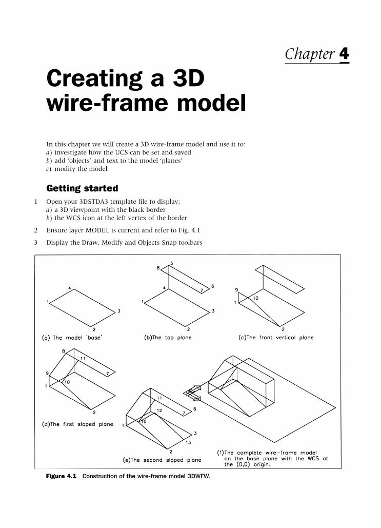
Creating a 3D wire-frame modelIn this chapter we will create a 3D wire-frame model and use it to:a) investigate how the UCS can be set and savedb) add ‘objects’ and text to the model ‘planes’c) modify the model
Getting started1 Open your 3DSTDA3 template file to display:
a) a 3D viewpoint with the black borderb) the WCS icon at the left vertex of the border
2 Ensure layer MODEL is current and refer to Fig. 4.1
3 Display the Draw, Modify and Objects Snap toolbars
Chapter 4
Figure 4.1 Construction of the wire-frame model 3DWFW.
modelling with AutoCAD.qxd 17/06/2002 15:37 Page 24

Creating the wire-frame model1 To create the base of the model – fig(a), select the LINE icon and draw:
Start point 50,50 <R> pt1Next point @200,0 <R> pt2Next point @0,120 <R> pt3Next point @–200,0 <R> pt4Next point close
2 The top plane – fig(b) is also created from lines, so with the LINE icon draw:Start point Intersection icon of pt4Next point @0,0,100 <R> pt5Next point @200,0,0 <R> pt6Next point @0,–40,0 <R> pt7Next point @–200,0,0 <R> pt8Next point Intersection icon of pt5 pt5Next point right-click and pick Enter
3 If you cannot ‘see’ the complete model, then menu bar with View-Zoom-Scale andenter a scale factor of 0.9
4 To create the front vertical plane – fig(c), select the LINE icon and draw:Start point Intersection icon of pt1Next point @0,0,45 <R> pt9Next point @60,0,0 <R> pt10Next point Intersection icon of pt2Next point right-click and Enter
5 With the LINE icon draw:Start point Intersection of pt9Next point Intersection of pt8 then right-click/enter
6 LINE icon again:Start point Intersection of pt10Next point Perpendicular to line 78 pt11Next point right-click and Enterand first sloped plane created – fig(d)
7 To create the second sloped plane – fig(e), select the LINE icon and draw:Start point Intersection of pt10Next point @0,80,0 <R> pt12Next point Perpendicular to line 23 pt13Next point right-click and Enter – fig(e)
8 To completing the model, three lines require to be added, so with the LINE icon draw:a) from pt3 to pt6b) from pt7 to pt13c) from pt11 to pt12
9 The completed model is displayed in fig(f) on ‘its base’, i.e. the black border.
10 At this stage save the model as a drawing file with the name C:\MODR2002\3DWFM
11 NoteThe model has been created using 3D coordinate input with the WCS, i.e. no attempthas been made to use the UCS. This is a perfectly valid method of creating wire-framemodels, but difficulty can be experienced if objects and text have to be added to thevarious ‘surfaces’ of the model when the coordinates need to be calculated. Using theUCS usually overcomes this type of problem.
Creating a 3D wire-frame model 25
modelling with AutoCAD.qxd 17/06/2002 15:37 Page 25

Moving around with the UCSTo obtain a better understanding of the UCS and how it is used with 3D models, we willuse the created wire-frame model to add some objects and text. The sequence is quitelong but it is important that you persevere and complete the exercise. Both menu barand keyboard entry methods will be used to activate the UCS command.
1 Open the wire-frame model C:\MODR2000\3DWFM or continue from the previousexercise. This model has the WCS icon at the black border origin point – the left vertex
2 Menu bar with View-Display-UCS Icon and:a) On and Origin both active (tick)b) select Properties and set a 2D UCS icon style
3 Refer to Fig. 4.2
4 PAN the layout until the lower black border vertex is near the lower edge of the screen.This will allow us to ‘see’ any UCS movements more clearly
5 Menu bar with Tools-New UCS-Origin and:prompt Specify new origin point<0,0,0>respond Intersection icon and pick pt1and a) icon ‘moves’ to selected point – fig(a)
b) it is a UCS icon – no Wc) it is at the origin – the +
note if the icon does not move to the selected point, menu bar with View-Display-UCS Icon and pick Origin
26 Modelling with AutoCAD 2002
Figure 4.2 Investigating the UCS and adding objects and text to 3DWFW.
modelling with AutoCAD.qxd 17/06/2002 15:37 Page 26

6 Now that the icon has been repositioned at point 1, we want to save its ‘position’ forfuture recall, so at the command line enter UCS <R> and:prompt Enter an optionenter S <R> – the save optionprompt Enter name to save current UCSenter BASE <R>
7 Make layer OBJECTS current and use the LINE icon to draw:Start point 100,25,0 <R>Next point @0,30,0 <R>Next point 145,40,0 <R>Next point close
8 Make layer TEXT current and menu bar with Draw-Text-Single Line Text and:a) start point: 60,10,0b) height: 10 and 0 rotationc) text item: BASE
9 The line objects and text item are added as fig(a)
10 Menu bar with Tools-New UCS-Origin and:prompt Specify new origin point<0,0,0>respond Intersection icon and pick pt8and icon ‘jumps’ to the selected point – fig(b)
11 At the command line enter UCS <R> and:prompt Enter an optionenter S <R> – the save optionprompt Enter name to save current UCSenter TOP <R>
12 With layer OBJECTS current draw a circle with centre: 60,20 and radius: 15
13 With layer TEXT current, add single line text using:a) start point: 85,10b) height: 10 with 0 rotationc) text item: TOP
14 Using the COPY icon:a) select objects: pick the circle then right-clickb) base point: Center icon and pick the circlec) second point: enter @0,0,–100 <R> – fig(b)d) question: why these coordinates?
15 Menu bar with Tools-UCS-3Point and:prompt Specify new origin point<0,0,0>respond Intersection icon and pick pt2prompt Specify point on positive portion of the X-axisrespond Intersection icon and pick pt3prompt Specify point on positive-Y portion of the UCS XY planerespond Intersection icon and pick pt10
16 The UCS icon will move to point 2 and be ‘aligned’ on the sloped surface as fig(c)
17 NoteThe 3 point option of the UCS command is ‘asking the user’ for three points to definethe UCS icon orientation, these being:first prompt the origin pointsecond prompt the direction of the X axisthird prompt the direction of the Y axis
Creating a 3D wire-frame model 27
modelling with AutoCAD.qxd 17/06/2002 15:37 Page 27

18 Save this UCS position by entering at the command line UCS <R> then S <R> and:prompt Enter name to save current UCSenter SLOPE1 <R>
19 With layer OBJECTS current use the LINE icon to draw:Start 15,100,0Next @50,0,0Next 40,30,0Next close
20 With layer TEXT current, add a single text item using:a) start point: centred on 10,110b) height: 10 with 0 rotationc) item: SLOPE1 – fig(c)
21 At command line enter UCS <R> and:prompt Enter an optionenter R <R> – the restore optionprompt Enter name of UCS to restoreenter BASE <R>and icon restored to the base point as fig(a)(The restore option is used extensively with UCS’s)
22 Menu bar with Tools-New UCS-X and:prompt Specify rotation angle about X axisenter 90 <R>and icon displayed as fig(d)
23 At command line enter UCS <R> then S <R> for the save option and FRONT <R>as the UCS name to save
24 With layer TEXT current add an item of text with:a) start point: 25,20b) height: 10 with 0 rotationc) text: FRONT – fig(d)
25 Menu bar with Tools-New UCS-3 Point and:prompt Specify new origin pointrespond Intersection icon and pick pt7prompt Specify point on positive portion of the X-axisrespond Intersection and pick pt11prompt Specify point on positive-Y portion of the UCS XY planerespond Intersection icon and pick pt13
26 The UCS icon will be aligned as fig(e)
27 Save this UCS position as VERT1 – easy? (UCS-S-VERT1)
28 With layer TEXT current add a text item with:a) start point: 120,50b) height: 10c) rotation: –90d) text: VERT1 – fig(e)
29 Restore UCS BASE and the model will be displayed as fig(f)
30 Make layer MODEL current and save the drawing at this stage as C:\MODR2000\3DWFM updating the original wire-frame model.
28 Modelling with AutoCAD 2002
modelling with AutoCAD.qxd 17/06/2002 15:37 Page 28

Modifying the wire-frame modelTo further investigate the UCS we will modify the wire-frame model, so refer to Fig. 4.3 and:
1 3DWFM still on the screen? – if not open the drawing file
2 Layer MODEL current with UCS BASE – fig(a)
3 Select the CHAMFER icon from the Modify toolbar and:a) set both chamfer distances to 30b) chamfer lines 7–11 and 7–13c) chamfer lines 5–6 and 6–3
4 Now add two lines to complete the ‘chamfered corner’ and erase the unwanted originalcorner line – fig(b).
5 Restore UCS VERT1 and note its position – fig(c)
6 Draw two circles:a) centre at 80,0,0 with radius 30b) centre at 80,0,–40 with radius 30 – fig(c)
7 Using the TRIM icon from the Modify toolbar:a) trim the two circles ‘above’ the modelb) trim the two lines ‘between’ the circles – fig(d)
8 Move the TOP text item from: ENDPOINT of pt5, by: @80,0
9 Draw in the two lines on the top plane and restore UCS BASE.
10 The modified model is now complete – fig(e)
11 Save the model as C:\MODR2000\3DWFM updating the existing model drawing
12 NoteThe user should realise that the UCS is an important concept with 3D modelling. IndeedI would suggest that 3D modelling would be very difficult (if not impossible) without it.
Creating a 3D wire-frame model 29
Figure 4.3 Modifying the 3DWFM model.
modelling with AutoCAD.qxd 17/06/2002 15:37 Page 29

Task 11 The wire-frame model has eleven flat planes and one ‘curved surface’. We have set and
saved UCS positions for five of these planes – BASE, TOP, SLOPE1, FRONT and VERT1.
2 You now have to set and save the other six flat UCS positions, i.e. one for each surfaceand add an appropriate text item to that surface.
3 My suggestions for the UCS name and text item are LEFT, RIGHT, REAR, SLOPE2,SLOPE3 and VERT2 but you can use any names that you consider suitable.
4 Figure 4.4 displays the complete wire-frame model with text added to every plane (withthe exception of the curved surface) using the UCS positions I ‘set’ Realise that youradditional text may differ in appearance from mine. This is acceptable as your UCSpositions may be ‘set’ different from mine
5 When complete, remember to save as MODR2002\3DWFM as it will be used in otherchapters.
Task 21 Restore UCS BASE – should be current?
2 With the MOVE command:a) window the complete model then right-clickb) base point: 0,0c) second point: @100,100
3 The complete model moves as expected, but do the set UCS’s move with the model? Thiscan be a nuisance when moving models. The UCS is ‘not tied’ to a specific model, it isONLY A POSITION ON THE SCREEN
4 This exercise is now complete. Do not save the changes.
Figure 4.4 The complete 3D wire-frame model (3DWFM) with text added to every plane.
30 Modelling with AutoCAD 2002
modelling with AutoCAD.qxd 17/06/2002 15:37 Page 30

Summary1 Wire-frame models are created by coordinate input and by referencing existing objects
2 Both the WCS and UCS entry modes can be used, but I would recommend:a) use the WCS to create the basic model outlineb) use the UCS to modify and add items to the model
3 It is strongly recommended that a UCS be set and saved for every surface on a wire-frame model.
AssignmentsCreating wire-frame models at this stage is important as it allows the user to:a) use 3D coordinate entry with the WCS and/or the UCSb) set and save different UCS positionsc) become familiar with the concept of 3D modelling
I have included two 3D wire-frame models which have to be created. The suggestedapproach is:
1 Open your 3DSTDA3 standard file – template or drawing
2 Complete the model with layer MODEL current, starting at some convenient point, e.g.50,50,0. Use WCS entry and add one ‘plane’ at a time
3 Save each completed model as a drawing file in your named folder with a suitable name,e.g. C\MODR2002\ACT2, etc.
4 Note:a) do not attempt to add dimensionsb) do not attempt to display the two models on ‘one screen’ – you will soon be able to
achieve this for yourself.c) these models will be used for later assignments, so ensure they are savedd) use your discretion for any sizes not given
The activities concern our master builder MACFARAMUS, and you have to create 3Dwire-frame models of two of his famous shaped blocks. It is not known how these blockswere used, i.e. in road building, structures, plazas etc, but they allow us to create wire-frame models.
Activity 2: MACFARAMUS’s shaped block 1
A relatively simple wire-frame model to create. I suggest that you construct it in a similarmanner to the worked example, i.e. create the base, then the front vertical plane. The‘back’ vertical plane can be drawn or copied from the front plane. The top and slopesare then easy to complete. When finished, save as MODR2002\ACT2
Activity 3: MACFARAMUS’s shaped block 2
This shaped block is slightly more difficult due to the curves. Create the basic shape astwo rectangular blocks, then add four circles, using an obvious ‘corner point’ as the circlecentre. The circles and lines can then be trimmed ‘to each other’, but the UCS positionis important. When complete, save as MODR2002\ACT3
Creating a 3D wire-frame model 31
modelling with AutoCAD.qxd 17/06/2002 15:37 Page 31

The UCSThe UCS is one of the basic 3D draughting ‘tools’ and it has several commands associatedwith it. Although it was used in the previous chapter, we will now investigate in more detail:a) setting a new UCS positionb) moving the UCSc) the UCS and UCS II toolbarsd) the UCS dialogue boxe) Orthographic UCSsf) UCS specific commands
Getting started1 Open your MODR2002\3DWFM model from the previous chapter. This model has several
blue objects with several saved UCS positions and is ‘positioned’ on the black ‘sheet border’
2 Restore the UCS BASE – probably is current?
3 Layer MODEL current and freeze layer TEXT. Refer to Fig. 5.1 which does not displaythe black sheet border. This is for clarity only.
Chapter 5
Figure 5.1 The UCS (NEW) options exercise.
modelling with AutoCAD.qxd 17/06/2002 15:37 Page 32

Setting a new UCS positionThe user can set a new UCS position from the menu bar with Tools-New UCS or byentering UCS <R> then N <R> at the command line. Both methods give the useraccess to the same options although the selection order differs. The menu bar optionsare displayed as:
World/Object/Face/View/Origin/ZAxis Vector/3 Point/X/Y/Z
The following is an explanation of these UCS option:
World1 This option restores the WCS setting irrespective of the current UCS position. It is the
default AutoCAD setting.
2 At the command line enter UCS <R> then W <R> to display the WCS icon on thesheet border at the left vertex as fig(a)
Origin1 Used to set a new origin point. The user specifies this new origin point by:
a) picking any point on the screenb) coordinate entryc) referencing existing objects
2 When used, the UCS icon is positioned at the selected point if the UCS Icon display isset to Origin. This option has been used in previous exercises.
3 Menu bar with Tools-New UCS-Origin and:prompt Specify new origin point<0,0,0>respond Intersection icon and pick ptAand icon positioned as fig(b)
Z Axis Vector1 Defines the UCS position relative to the Z axis, the user specifying:
a) the origin pointb) any point on the Z axis
2 Menu bar with Tools-New UCS-Z Axis Vector and:prompt Specify new origin pointrespond Intersection icon and pick ptBprompt Specify point on positive portion of Z-axisrespond Intersection icon and pick ptC – fig(c)
3 The icon will be aligned with:a) the X axis along the shorter base left edgeb) the Y axis along the front left vertical edgec) the Z axis along the line BC
The UCS 33
modelling with AutoCAD.qxd 17/06/2002 15:37 Page 33

3 Point 1 Defines the UCS orientation by specifying three points:
a) the actual origin pointb) a point on the positive X axisc) a point on the positive Y axis
2 Menu bar with Tools-New UCS-3 Point and:prompt Specify new origin point respond Intersection of ptBprompt Specify point on positive portion of the X-axisrespond Intersection of ptCprompt Specify point on positive-Y portion of the UCS XY planerespond Intersection of ptD – icon as fig(d)
3 This is a very useful option especially if the icon is to be aligned on sloped surfaces. Itis probably my preferred method of setting the UCS.
Object1 Aligns the icon to an object, e.g. a line, circle, polyline, item of text, dimension, block etc.
2 Menu bar with Tools-New UCS-Object and:prompt Select object to align UCSrespond pick any point on circle on top surface
3 The icon is aligned as fig(e) with:a) the origin at the circle centre pointb) the positive X axis pointing towards the circumference of the circle at the point
‘picked’ by the user
View1 Aligns the UCS so that the XY plane is always perpendicular to the view plane.
2 Menu bar with Tools-New UCS-View
3 The UCS icon will be displayed as fig(f) and is similar to the traditional 2D icon?
4 This is a useful UCS option as it allows 2D text to be added to a 3D drawing – try it foryourself.
X/Y/Z1 Allows the UCS to be rotated about the entered axis by an amount specified by the user
2 Make UCS BASE current
3 Menu bar with Tools-New UCS-X and:prompt Specify rotation angle about the X axisenter 90 <R> – fig(g)
4 Menu bar with Tools-New UCS-Y and:prompt Specify rotation angle about the Y axisenter –90 <R> – fig(h)
5 Menu bar with Tools-New UCS-Z and:prompt Specify rotation angle about the Z axisenter –90 <R> – fig(i)
34 Modelling with AutoCAD 2002
modelling with AutoCAD.qxd 17/06/2002 15:37 Page 34

Face1 Aligns the UCS with a selected solid model face. This option cannot be used with 3D wire-
frame models.
2 Restore UCS BASE
3 Menu bar with Tools-New UCS-Face and:prompt Select face of solid objectrespond pick any line of the top planeprompt A 3D solid must be selected
No solids detected
ApplyAn option which allows the user to apply the current UCS setting to a specific viewport.We will use this option in later chapters, but not yet.
Moving a UCSA selection which allows the user to move the UCS to a new origin position, the UCSicon retaining both its orientation and name. Refer to Fig. 5.1 and:
1 UCS restored to BASE
2 Menu bar with Tools-Move UCS and:prompt Specify new origin point or [Zdepth]respond Intersection icon and pick ptAand icon moved to point A and retains the name BASE
3 Restore UCS TOP
4 At the command line enter UCS <R> and:prompt Enter an option [New/Move/..enter M <R> – the move optionprompt Specify new origin point or [Zdepth]respond Intersection icon and pick ptCand icon moves to point C and retains the name TOP
5 Restore UCS FRONT
6 Menu bar with Tools-Move UCS and:prompt Specify new origin point or [Zdepth]enter Z <R> – the Z depth optionprompt Specify Zdepth<0>enter –120 <R>and icon moved to ‘back of model’ and retains name FRONT
7 Note:a) This UCS command should be used with caution as the user may not want a named
UCS to be ‘repositioned’b) I never use this command. If I want to reposition the UCS, I use the origin optionc) Do not save the drawing, as you will saved these moved UCS’s
8 TaskReset the three moved UCS’s to their original positions, i.e. BASE, TOP and FRONT
The UCS 35
modelling with AutoCAD.qxd 17/06/2002 15:37 Page 35

Other UCS optionsThe new UCS options are available from the command line but the menu bar selectionTools-New UCS is the usual method of activating the command. The command line hasother UCS options available for selection, these being:
Prev1 Restores the previously ‘set’ UCS position and can be used to restore the last 10 UCS
positions.
2 The command is activated from the command line by entering UCS <R> then P <R>and can be used continually until the command line displays ‘no previous coordinate systemsaved’.
Restore1 Allows the user to restore a previously saved UCS position but the names of the saved
UCS’s must be remembered (This will be modified shortly). This option has been usedin our examples
2 At the command line enter UCS <R> then R <R> and:prompt Enter name of UCS to restore or [?]enter TOP <R>then restore UCS BASE
Save1 Allows the user to save a UCS position for future recall. It should be used every time a
new UCS has been defined.
2 The option is activated from the command line with UCS <R> then S <R> and theuser can enter any name for the UCS position.
Del1 Entering UCS <R> then D <R> prompts for the UCS name to be deleted.
2 The default is none. Use with care!
?1 The query option which will list all saved UCS positions
2 At the command line enter UCS <R> then ? <R> and:prompt Enter UCS name(s) to list<*>respond press the RETURN keyprompt AutoCAD Text Window with:
Current UCS Name: BASESaved Coordinate systems
and Details about all the saved UCS’s, their origin point and their X,Y and Z axesorientation
respond cancel the window
36 Modelling with AutoCAD 2002
modelling with AutoCAD.qxd 17/06/2002 15:37 Page 36

The UCS toolbarAll the UCS options have so far been activated by keyboard entry with UCS <R> orfrom the menu bar with Tools. The only reason for this is that I think it easier for theuser to understand what option is being used. The UCS options can also be activated inicon form from the UCS and UCS II toolbars – Fig. 5.2. The toolbars have no icon selectionfor the orthographic options or for Restore, Save, Delete or for query (?), although thesecan easily be activated by selecting the actual UCS icon. An additional icon in both theUCS and UCS II toolbars is Display UCS Dialog, while the UCS II toolbar allows savedUCS’s to be made current, i.e. restored.
The user now has three methods of activating the various UCS options, these being:a) from the menu barb) by command line entryc) in icon form from the appropriate toolbar
It is user preference as to what method is used.
The UCS 37
Figure 5.2 The UCS and UCS II toolbars.
World UCSUCS Previous
Display UCS DialogUCS
Origin UCSZ Axis Vector UCS
3 Point UCSX Axis Rotate UCS
Object UCSFace UCS
View UCS
Apply UCSZ Axis Rotate UCS
Y Axis Rotate UCS
Saved UCS’s
Display UCS dialogMove UCS
modelling with AutoCAD.qxd 17/06/2002 15:37 Page 37

The UCS dialogue box The UCS dialogue box can be activated by three different methods:a) from the menu bar with Tools-Named UCSb) by selecting the Display UCS dialog icon from either the UCS or UCS II toolbarc) by entering UCSMAN <R> at the command line
When activated, the dialogue box allows the user three tab selections, these being:a) Named UCSs – the defaultb) Orthographic UCSsc) Settings
To demonstrate using the UCS dialogue box:
1 Ensure the 3DWFM is displayed with UCS BASE current
2 Menu bar with Tools-Named UCS and:prompt UCS dialogue boxwith three tab selections and Named UCSs tab activeand a) a list of saved UCS names for the model
b) a World and Previous selection optionrespond 1. pick Top
2. pick Set Current – Fig. 5.33. pick OK
2 The model will be displayed with the icon at the TOP setting
3 Use the Named UCS tab of the UCS dialogue box to set current some other saved UCSpositions
4 Set UCS BASE current
38 Modelling with AutoCAD 2002
Figure 5.3 The UCS dialogue box – Named UCS tab.
modelling with AutoCAD.qxd 17/06/2002 15:37 Page 38

5 Activate the UCS dialogue box and:prompt UCS dialogue box – Named UCS tab activerespond 1. pick TOP and it becomes highlighted
2. right-click the mouseprompt shortcut menu with selections for: Set Current, Rename, Delete, Detailsrespond 1. pick Rename
2. enter new name: ABOVE <R>3. pick Set Current4. pick OK
6 The UCS will be displayed in the ‘old top position’
7 Now:a) rename the ABOVE UCS to TOP againb) make UCS BASE current
8 Activate the UCS dialogue box and pick the Settings tab and:prompt Settings tab – Fig. 5.4with 1. UCS icon settings for ON and ORIGIN – both active
2. UCS settings for viewports and planrespond note the settings then pick Cancel
9 Notea) The UCS icon settings from the dialogue box are the same as the menu bar selection
of View-Display-UCS Icon-On/Originb) The other Settings options will be discussed in later chapters
The UCS 39
Figure 5.4 The UCS dialogue box – Settings tab.
modelling with AutoCAD.qxd 17/06/2002 15:37 Page 39

Setting an orthographic UCSThis allows the user to restore six preset UCS positions, the orientation being set relativeto a saved UCS. Refer to Fig. 5.5 and:
1 Ensure the 3DWFM is displayed with the saved UCSs
2 Restore UCS SLOPE1 current – fig(a)
3 Activate the UCS dialogue box with the Orthographic UCS tab active and:prompt UCS dialogue box – Orthographic tab displayrespond 1. scroll at Relative to
2. pick BASE3. at Current UCS Name, pick TOP4. pick Set Current – Fig. 5.65. pick OK
and icon displayed as fig(b)
4 With the Orthographic tab of the UCS dialogue box, set Bottom current relative to BASE– fig(c)
5 Menu bar with Tools-Orthographic UCS-Left to display the icon as fig(d)
40 Modelling with AutoCAD 2002
Figure 5.5 The Orthographic UCS options exercise relative to BASE with UCS SLOPE1 current.
modelling with AutoCAD.qxd 17/06/2002 15:37 Page 40
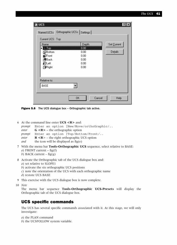
6 At the command line enter UCS <R> and:prompt Enter an option [New/Move/orthoGraphic/..enter G <R> – the orthographic optionprompt Enter an option [Top/Bottom/Front/..enter R <R> – the right orthographic UCS optionand the icon will be displayed as fig(e)
7 With the menu bar Tools-Orthographic UCS sequence, select relative to BASE:a) FRONT current – fig(f)b) BACK current – fig(g)
8 Activate the Orthographic tab of the UCS dialogue box and:a) set relative to SLOPE1b) activate the six orthographic UCS positionsc) note the orientation of the UCS with each orthographic named) restore UCS BASE
9 This exercise with the UCS dialogue box is now complete.
10 NoteThe menu bar sequence Tools-Orthographic UCS-Presets will display theOrthographic tab of the UCS dialogue box.
UCS specific commandsThe UCS has several specific commands associated with it. At this stage, we will onlyinvestigate:
a) the PLAN commandb) the UCSFOLLOW system variable.
The UCS 41
Figure 5.6 The UCS dialogue box – Orthographic tab active.
modelling with AutoCAD.qxd 17/06/2002 15:37 Page 41

PlanPlan is a command which displays any model perpendicular to the XY plane of thecurrent UCS position.
1 Ensure the 3DWFM is displayed with UCS BASE current
2 Refer to Fig. 5.7
3 At the command line enter PLAN <R> and:prompt Enter an option [Current ucs/Ucs/World] <Current>enter <R> i.e. accept the Current UCS default
4 The screen will display the model as a plan view – fig(a). This view is perpendicular tothe current UCS setting (BASE) and is really a ‘top’ view in orthogonal terms
5 Restore UCS FRONT – pencil icon?
6 Menu bar with View-3D Views-Plan View-Current UCS and the model will bedisplayed as fig(b). This is a plan view to the current UCS FRONT and is a ‘front’ viewin orthogonal terms
7 Menu bar with View-3D Views-Plan View-Named UCS and:prompt Enter name of UCSenter SLOPE1 <R>
8 The model will be displayed as a plan to the UCS SLOPE1 setting as fig(c)
9 At the command line enter PLAN <R> and:prompt Enter an option [Current ucs/Ucs/World]<Current>enter U <R> – the Ucs optionprompt Enter name of UCSenter VERT1 <R>
42 Modelling with AutoCAD 2002
Figure 5.7 The PLAN command with 3DWFM.
modelling with AutoCAD.qxd 17/06/2002 15:37 Page 42
10 The model display is as fig(d) i.e. a plan view to the UCS setting VERT1. This displayshould be upside-down – why?
11 Finally restore UCS BASE and menu bar with View-3D Views-SE Isometric to return theoriginal model display.
UCSFOLLOWUCS FOLLOW is a system variable which controls the screen display of a model whenthe UCS position is altered. The variable can only have the values of 0 (default) or 1 and:a) UCSFOLLOW 0: no effect on the display with UCS changesb) UCSFOLLOW 1: automatically generates a plan view when the UCS is altered
1 Original 3D display with UCS BASE on the screen?
2 At the command line enter UCSFOLLOW <R> and:prompt Enter new value for UCSFOLLOW <0>enter 1 <R>
3 Nothing has changed?
4 Restore UCS FRONT – plan view as Fig. 5.7(b)
5 Restore UCS SLOPE1 – plan view as Fig. 5.7(c)
6 Restore UCS VERT1 – plan view as Fig. 5.7(d)
7 Restore UCS BASE – plan view as Fig. 5.7(a)
8 Set UCSFOLLOW to 0 and restore the original screen display with View-3D Views-SEIsometric
9 This completes the exercises with the UCS
Summary1 The UCS is an essential 3D modelling aid
2 The UCS command has several options including:a) New: origin, 3 point, X,Y,Z rotateb) Move: which should be used with cautionc) Orthographic: six preset UCS settings
3 The orientation of the UCS icon is dependent on the option used
4 The UCS toolbars offer fast option selection
5 It is STRONGLY RECOMMENDED that the UCS icon and the UCS icon origin are ONwhen working in 3D. These can be activated with:a) the menu bar sequence View-Display-UCS Iconb) the Settings tab of the UCS dialogue box
6 The UCS dialogue box allows flexible management of the UCS with three tab selections:a) Named UCSs – set current, rename, deleteb) Orthographic UCSs (Presets)c) Settings
7 PLAN is a command which displays the model perpendicular to the XY plane of thecurrent UCS
8 UCSFOLLOW is a system variable which can be set to give automatic plan views whenthe UCS is re-positioned. It is recommended that this variable be set to 0, i.e. off.
The UCS 43
modelling with AutoCAD.qxd 17/06/2002 15:37 Page 43

The modify commandswith 3D modelsAll the modify commands are available for use with 3D models, but the results aredependent on the UCS position. We will investigate how the COPY, ARRAY, ROTATEand MIRROR commands can be used with our 3D wire-frame model so:
1 Open your 3DWFM model with UCS BASE and layer MODEL current
2 Display the Modify, Object snap and UCS toolbars
3 Erase all text but the FRONT text item
The COPY command1 Select the COPY icon from the Modify toolbar and:
prompt Select objectsrespond pick the 4 red lines and the green FRONT text item on the ‘front
vertical’ plane then right-clickprompt Specify base point or displacementrespond Intersection icon and pick ptAprompt Specify second point of displacemententer @0,0,260 <R> – Fig. 6.1.A(a)
Chapter 6
Figure 6.1 The COPY and ARRAY commands with 3DWFM.
modelling with AutoCAD.qxd 17/06/2002 15:37 Page 44

2 Restore UCS FRONT
3 Select the COPY icon and:prompt Select objectsenter P <R><R> – previous selection set optionprompt Specify base point and: pick Intersection of ptAprompt Specify second point and enter: @0,0,260 <R> – Fig. 6.1.A(b)
4 Menu bar with View-Zoom-All
5 Undo (or erase) the copied effects to leave the original model
The ARRAY command1 Restore UCS BASE
2 At the command line enter –ARRAY <R> and:prompt Select objectsrespond pick the FRONT text item then right-clickprompt Enter the type of array and enter: R <R>prompt Enter the number of rows and enter: 2 <R>prompt Enter the number of columns and enter: 6 <R>prompt Enter the row distance and enter: 40 <R>prompt Specify the distance between columns and enter: 60 <R>
3 The text item is arrayed in a 2×6 rectangular matrix as Fig. 6.1.B(a)
4 Restore UCS SLOPE1
5 Rectangular array the original FRONT text item using the same entries as step 2 – Fig. 6.1.B(b)
6 Undo (or erase) the arrayed effects
The ROTATE command1 Restore UCS BASE
2 Select the ROTATE icon from the Modify toolbar and:prompt Select objectsrespond pick the 4 red lines and the FRONT text item as before then right-clickprompt Specify base pointrespond Intersection icon and pick ptAprompt Specify rotation angleenter 90 <R>
3 The selected objects will be rotated as Fig. 6.2.A(a)
4 Undo this rotated effect
5 Restore UCS FRONT and rotate the same objects with the same entries as step 2. Thiswill give Fig. 6.2.A(b)
6 Undo this effect
The modify commands with 3D models 45
modelling with AutoCAD.qxd 17/06/2002 15:37 Page 45

The MIRROR command1 Restore UCS BASE, activate the Mirror icon and:
prompt Select objectsrespond pick the four lines and text item as before and right-clickprompt Specify first point of mirror linerespond Intersection icon and pick ptAprompt Specify second point of mirror linerespond Intersection icon and pick ptBprompt Delete source objectsenter N <R>
2 The selected objects will be mirrored about the line AB as Fig. 6.2.B(a)
3 Restore UCS SLOPE1 and repeat the mirror command with the same objects and sameentries as step 1. This will give Fig. 6.2.B(b)
Other modify commandsAll of the modify commands are available for use with 3D models, but the final resultis dependent on the UCS position. The only requirement for the user is to ensure thatthe icon is positioned on the ‘plane’ for the modification.
SummaryThe AutoCAD modify commands with 3D models have to be used with care. The resultis UCS dependent.
46 Modelling with AutoCAD 2002
Figure 6.2 The ROTATE and MIRROR commands with 3DWFM.
modelling with AutoCAD.qxd 17/06/2002 15:37 Page 46

Dimensioning in 3DThere are no special commands to add dimensions in 3D. Dimensioning is a 2D concept,the user adding the dimensions to the XY plane of the current UCS setting. This meansthat the orientation of the complete ‘dimension object’ will depend on the UCS position.The user should be aware of:a) AutoCAD’s automatic dimensioning facilityb) linear dimensioning will be horizontal or vertical, depending on where the
dimension line is located in relation to the object being dimensioned.
We will demonstrate how dimensions can be added to 3D models with two examples.The first will be the 3D wire-frame model 3DWFM, and the second will use AutoCAD’sstored 3D objects.
Example 11 Open MODR2002\3DWFM and display the Dimension, Object Snap and other toolbars
to suit
2 Freeze layer TEXT and make layer DIM current
3 The standard sheet created as the template/drawing file had a created dimension style– 3DSTD. You may want to ‘alter’ the Overall Scale (Fit tab) to a value of 1.5 which willmake the added dimensions ‘clearer’
4 Ensure UCS BASE is current and refer to Fig. 7.1
Chapter 7
Figure 7.1 Dimension exercise with 3DWFM.
modelling with AutoCAD.qxd 17/06/2002 15:37 Page 47

5 Select the LINEAR dimension icon and:prompt Specify first extension line originrespond Intersection icon and pick pt1prompt Specify second extension line originrespond Intersection icon and pick pt2prompt Specify dimension line locationrespond pick to suit
6 Repeat the LINEAR dimension selection and dimension line 23, positioning thedimension line to suit
7 Select the DIAMETER icon and:prompt Select circle or arcrespond pick the circle on the TOP ‘plane’prompt Specify dimension line locationrespond pick to suit – interesting result?
8 The three added dimensions will be displayed as fig(a)
9 Erase the added dimensions and restore UCS FRONT
10 Using the dimension icons:a) linear dimension lines 12 and 14b) align dimension line 56c) try and add a diameter dimension to the top circled) dimensions displayed as fig(b)
11 Erase these added dimensions and restore UCS TOP and:a) linear dimension line 67 and line 78b) diameter dimension the circle on the topc) result as fig(c)
12 Restore UCS SLOPE1, erase the previous dimensions and:a) linear dimension line 23 and line 29b) angular dimension a vertex of the blue triangle ‘on the slope’c) the three dimensions will be displayed as fig(d)
13 With UCS VERT1 current, erase the dimensions from SLOPE1 and:a) linear dimension line 67 and line 35b) align dimension line 56c) interesting result as fig(e) – why?
14 This exercise should demonstrate to the user that:a) adding dimensions to a 3D model is VERY UCS DEPENDENTb) there are no special 3D dimension commandsc) the actual orientation of added dimensions depends on the UCS position and
orientationd) dimensions are added to the XY plane of the current UCS
15 Task a) erase any dimensions still displayedb) with layer DIM current refer to Fig. 7.2 and add the given to the modelc) some of the existing saved UCS positions will be usedd) you may have to set a new UCS position for the continuous 80,40 and the 70
dimensionse) when complete save if required, but not as 3DWFM
48 Modelling with AutoCAD 2002
modelling with AutoCAD.qxd 17/06/2002 15:37 Page 48

Example 21 Close any existing drawings then menu bar with File-New and:
a) pick Use a Templateb) pick 3DSTDA3.dwt (your 3D template file) then pick OK
2 The screen will display the black border:a) in SE Isometric viewpointb) layer MODEL currentc) WCS icon at left vertex of border
3 Display the Surfaces toolbar and refer to Fig. 7.3
Dimensioning in 3D 49
Figure 7.2 Required dimensions to be added to 3DWFM.
Figure 7.3 Adding dimensions to 3D objects.
modelling with AutoCAD.qxd 17/06/2002 15:38 Page 49

4 Menu bar with Draw-Surfaces-3D Surfaces and:prompt 3D Objects dialogue boxrespond pick Box3d then OKprompt Specify corner of box and enter: 50,50,0 <R>prompt Specify length of box and enter: 120 <R>prompt Specify width of box or [Cube] and enter: 80 <R>prompt Specify height of box and enter: 60 <R>prompt Specify rotation of box about Z axis and enter: 0 <R>
4 Select the WEDGE icon from the surface toolbar and:prompt Specify corner of wedge and enter: 200,150,0 <R>prompt Specify length of box and enter: 100 <R>prompt Specify width of box and enter: 75 <R>prompt Specify height of box and enter: 65 <R>prompt Specify rotation of wedge about Z axis and enter: 0 <R>
5 Using the 3 point UCS option:a) origin at point 1b) x axis along line 12c) y axis along line 13d) save UCS position as POS1e) add two linear dimensions with this UCS
6 Use the 3 point UCS option again with:a) origin at point ab) x axis along line abc) y axis along line acd) save as POS2e) add two linear dimensions with this UCS
7 Now add the three other dimensions, i.e. one to the box and two to the wedge. SomeUCS manipulation is required but you should manage this without any problems.
8 Menu bar with Tools-New UCS-World to return to the WCS.
9 TaskAnother 3D object has to be created and dimensioned so select the pyramid icon fromthe Surfaces toolbar and:prompt Specify first corner point for base of pyramid and enter:
40,220 <R>prompt Specify second corner point for base of pyramid and enter:
80,250 <R>prompt Specify third corner point for base of pyramid and enter:
60,320 <R>prompt Specify fourth corner point for base of pyramid or
[Tetrahedron]enter T <R> – the tetrahedron optionprompt Specify apex point of tetrahedronenter 60,320,75 <R>
10 Now set appropriate UCS positions and add the three linear dimensions given
11 Save if required, but the drawing will not be used again
50 Modelling with AutoCAD 2002
modelling with AutoCAD.qxd 17/06/2002 15:38 Page 50
Summary1 There are no special 3D dimension commands
2 Dimensioning is a 2D concept and dimensioning a 3D model involves adding thedimensions to the XY plane of the required UCS setting
3 If the UCS is not positioned correctly, dimensions can have the ‘wrong orientation’ inrelation to the object being dimensioned.
AssignmentTwo dimensioning assignments for you to complete, one being an existing wire-framemodel, the other being a new wire-frame model. Both involve the work of our greatarchitect MACFARAMUS.
Activity 4: Shaped block of MACFARAMUS
Recall the shaped block from activity 2 and:a) set and save appropriate UCS positionsb) add the given dimensionsc) save the completed model for later recall
Activity 5: The famous rectangular topped pyramid of MACFARAMUS
The rectangular topped pyramid designed by Macfaramus was never built but his designis still considered unique. You have to:a) create a wire-frame model of the pyramid using the sizes givenb) set and save several UCS positions, these being on the following surfaces:
1. the base and top – UCS BASE and UCS TOP2. the four ‘sides’ of the pyramid, which I have names as SLOPE1, SLOPE2, SLOPE3
and SLOPE4 (I know that two of these sides are not sloped, I named them in alogical order)
3. the vertical sides of the top. Use your own names, e.g. V1, etc.c) add the given dimensionsd) save the completed model
MACFARAMUS had to calculate certain angles and distances without the aid ofcalculators or computers. This took him a great deal of time and involved using hisknowledge of trigonometry. The angles and distances he required were:1. the angle of the two sloped ‘planes’ in relation to the base2. the length of the three sloped ‘edges’
His calculations gave the following values:a) angle of first sloped plane to the base: 50.19b) angle of second sloped plane to the base: 56.31c) length of the three sloped edges:
1 – 234.312 – 263.253 – 216.33
Was he correct?
Dimensioning in 3D 51
modelling with AutoCAD.qxd 17/06/2002 15:38 Page 51
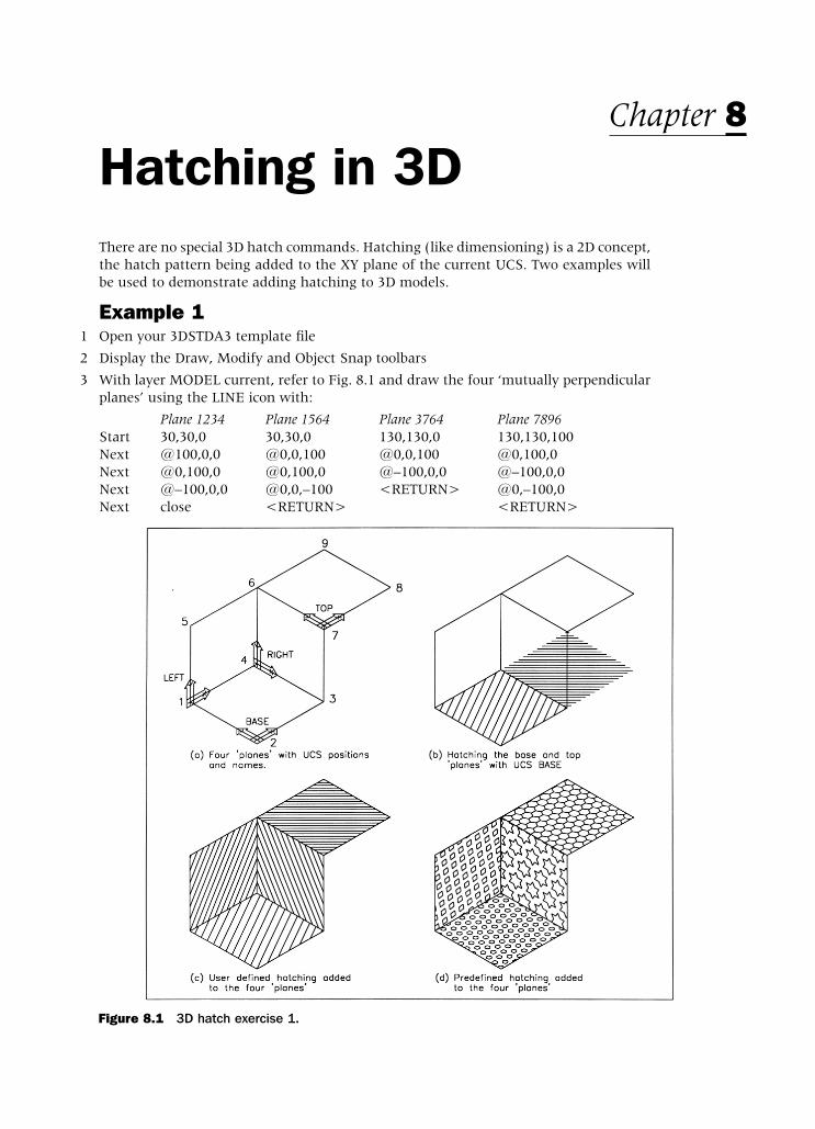
Hatching in 3DThere are no special 3D hatch commands. Hatching (like dimensioning) is a 2D concept,the hatch pattern being added to the XY plane of the current UCS. Two examples willbe used to demonstrate adding hatching to 3D models.
Example 11 Open your 3DSTDA3 template file
2 Display the Draw, Modify and Object Snap toolbars
3 With layer MODEL current, refer to Fig. 8.1 and draw the four ‘mutually perpendicularplanes’ using the LINE icon with:
Plane 1234 Plane 1564 Plane 3764 Plane 7896Start 30,30,0 30,30,0 130,130,0 130,130,100Next @100,0,0 @0,0,100 @0,0,100 @0,100,0Next @0,100,0 @0,100,0 @–100,0,0 @–100,0,0Next @–100,0,0 @0,0,–100 <RETURN> @0,–100,0Next close <RETURN> <RETURN>
Chapter 8
Figure 8.1 3D hatch exercise 1.
modelling with AutoCAD.qxd 17/06/2002 15:38 Page 52

4 Erase the black border and pan the drawing to suit
5 Set and save the four UCS positions as fig(a)
6 Restore UCS BASE and make SECT the current layer
7 Select the HATCH icon from the Draw toolbar and using the Boundary Hatch dialogue box:a) pick User defined pattern typeb) set angle to 30 and spacing to 8c) use the Pick Points< option and:
1. select a point within the 1234 plane then right-click/enter2. Preview-right click-OK
8 Repeat the HATCH icon selection and:a) using the Pick Points option pick a point within the 6789 plane and:
prompt Boundary Definition Error dialogue box – Fig. 8.2respond pick OK then <RETURN>
b) using the Select Objects option pick the four lines of the 6789 plane then right-click/enter and:1. set angle to –45 and spacing to 52. Preview-right click-OK
9 The result of the two hatch operations is displayed in fig(b) with plane 1234 having thecorrect hatching, but plane 6789 has none, the hatching having been added to the planeof UCS BASE.
10 Use the HATCH icon and try and add hatching to the vertical planes 1564 and 3467.a) Not possible? b) Unable to hatch the boundary message at the command linec) Why is this?
11 Erase the ‘wrong’ hatching and restore UCS TOP
12 Hatch the top plane (6789) using the HATCH icon with:a) pick points optionb) angle –45 and spacing 5
13 Add hatching to the two vertical planes remembering to restore UCS LEFT and UCSRIGHT – fig(c). Use your own angle and spacing values.
14 Taska) Erase the added hatching then add the following predefined hatch patterns using the
information given:UCS Pattern Scale AngleBASE HEX 1 –10TOP HONEY 2 0LEFT SQUARE 2 10RIGHT STARS 2 0
c) the result is fig(d)d) this completes example 1 which does not have to be saved.
Hatching in 3D 53
Figure 8.2 The Boundary Definition Error Message box.
modelling with AutoCAD.qxd 17/06/2002 15:38 Page 53

Example 21 Open the drawing C:\MODR2002\3DWFM and refer to Fig. 8.3
2 a) erase all text and any dimensionsb) erase the smaller triangle and lower circle on the base planec) make layer SECT currentd) restore UCS TOP
3 Select the HATCH icon and:a) Predefined pattern type: scroll and pick STARSb) set scale to 1 and angle to 0c) select Pick Points: pick internal points in the TWO top planes then right-click/enterd) preview-right click-OK
4 Restore UCS FRONT and with the HATCH icon:a) pattern type: ZIGZAGb) scale: 1.5 and angle: 30c) select objects: pick the four lines of front vertical plane then right-click/enterd) preview-right click-OK
5 Repeat the HATCH icon selection and add the following hatch patterns:UCS Pattern Scale Angle Selection typeSLOPE1 TRIANG 1 25 pick pointsVERT1 HOUND 2.5 0 pick points
6 Menu bar with View-Hide and the model is as before. Hatching a wire-frame modeldoes not produce a hide effect.
7 Save your completed hatched model but not as MODR2002/3DWFM.
8 NoteIn the two hatch exercises we used the one layer (SECT) for all hatching. It is sometimesdesirable to have a different layer for each current UCS that is to be used for hatching.This is a user decision.
54 Modelling with AutoCAD 2002
Figure 8.3 Hatch exercise with 3DWFM.
modelling with AutoCAD.qxd 17/06/2002 15:38 Page 54

Summary1 Hatching is a 2D concept
2 Hatching a 3D model requires the UCS to be set to the ‘plane’ which is to be hatched
3 a) both user-defined and pre-defined hatch patterns can be usedb) both the select objects and pick points methods are permitted
4 Hatching a 3D wire-frame model does not produce a hide effect
AssignmentsTwo hatch activities have been included, both using previously created wire-framemodels these being MACFARAMUS’s shaped block and rectangular topped pyramid.
The procedure with both activities is to:
1 Open the saved drawing
2 Freeze layer DIM, or erase the dimensions if necessary
3 Add appropriate hatching, making new hatch layers for each UCS position if required –your decision!
4 Use the pick points method where possible
5 Save the completed model.
Activity 6: The shaped block of MACFARAMUS
1 Restore the appropriate UCS and add the following user defined hatching:UCS Angle SpacingFRONT 45 8RIGHT 45 8MID 45 8SLOPE 45 8
2 When complete save the model as MODR2002\SHBLOCK for recall.
Activity 7: The rectangular topped pyramid of MACFARAMUS.
1 Using the correct UCS, add the following predefined hatch patterns:UCS Pattern Scale Anglefour ‘shaped’ planes BRICK 2 0four vert ‘top’ planes BRSTONE 1 0the horiz top surface EARTH 1.5 0
2 Save the complete hatched model as MODR2002\PYRAMID
3 Note:a) extra lines required for the hatch effect?b) the viewpoint has been altered for effect.
Hatching in 3D 55
modelling with AutoCAD.qxd 17/06/2002 15:38 Page 55
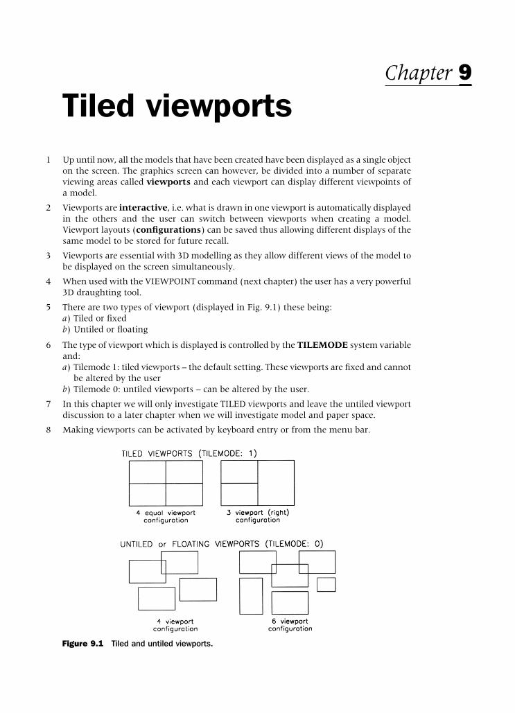
Tiled viewports1 Up until now, all the models that have been created have been displayed as a single object
on the screen. The graphics screen can however, be divided into a number of separateviewing areas called viewports and each viewport can display different viewpoints ofa model.
2 Viewports are interactive, i.e. what is drawn in one viewport is automatically displayedin the others and the user can switch between viewports when creating a model.Viewport layouts (configurations) can be saved thus allowing different displays of thesame model to be stored for future recall.
3 Viewports are essential with 3D modelling as they allow different views of the model tobe displayed on the screen simultaneously.
4 When used with the VIEWPOINT command (next chapter) the user has a very powerful3D draughting tool.
5 There are two types of viewport (displayed in Fig. 9.1) these being:a) Tiled or fixedb) Untiled or floating
6 The type of viewport which is displayed is controlled by the TILEMODE system variableand:a) Tilemode 1: tiled viewports – the default setting. These viewports are fixed and cannot
be altered by the userb) Tilemode 0: untiled viewports – can be altered by the user.
7 In this chapter we will only investigate TILED viewports and leave the untiled viewportdiscussion to a later chapter when we will investigate model and paper space.
8 Making viewports can be activated by keyboard entry or from the menu bar.
Chapter 9
Figure 9.1 Tiled and untiled viewports.
modelling with AutoCAD.qxd 17/06/2002 15:38 Page 56

Example 1 This exercise is rather long, but persevere with it.
1 Open your 3DWFM drawing of the wire-frame model on the black border with layerMODEL current and UCS BASE.
2 Deactivate all floating toolbars and display the model without any text, dimensions orhatching. Erase or freeze layers?
3 At the command line enter TILEMODE <R> and:prompt Enter new value for TILEMODE<1>and observe the 1 default then press ESC
4 The TILEMODE value of 1 indicates that only TILED viewports can be used. The samecondition is also evident with:a) Status bar: word MODEL is displayedb) Menu bar: View-Viewports indicate that Polygonal Viewport and Object are not
available for selection
5 Menu bar with View-Viewports-3 Viewports and:prompt Enter a configuration [Horizontal/Vertical/Above..enter R <R> – the right configuration option
6 The drawing screen will:a) be divided into three separate ‘areas’ – one large at the right and two smaller to the
left. The three viewports will ‘fill the screen’ as Fig. 9.2(a)b) display the same view of the model in the three viewports
Tiled viewports 57
Figure 9.2 Viewport example 1.
modelling with AutoCAD.qxd 17/06/2002 15:38 Page 57

7 Move the mouse about the screen and:a) the large viewport will display the cursor cross-hairs and is the ACTIVE viewport,
i.e. it is ‘current’b) the other viewports will display an arrow and these viewports are NON-ACTIVE
8 Any viewport can be made active by:a) moving the mouse into the viewport areab) left-clickc) try this for yourself a few times
9 At the command line enter -VPORTS <R> and:prompt Enter an option [Save/Restore/Delete/..enter S <R> – the save optionprompt Enter name for new viewport configurationenter CONF1 <R>
10 Make the upper left viewport active and select the menu bar sequence View-Viewports-2 Viewports and:prompt Enter a configuration option [Horizontal/Vertical..enter V <R> – the vertical optionand the top left viewport will be further divided into two equal vertical viewports,
each displaying the model layout
11 Make the lower left viewport active and menu bar with View-Viewports-4 Viewportsto display an additional four viewports of the model
12 At the command line enter -VPORTS <R> and:prompt Enter an option [Save/Restore/..enter S <R> – the save optionprompt Enter name for new viewport configurationenter CONF2 <R>
13 With the lower left viewport active, enter -VPORTS <R> at the command line and:prompt Enter an option [Save/Restore..enter 3 <R> – the 3 viewport optionprompt Enter a configuration option [Horizontal/Vertical/Above..enter H <R> – the horizontal option
14 The lower left viewport will be further divided into another three viewports and at thisstage your screen should resemble Fig. 9.2(b)
15 Make the lower left viewport active and enter -VPORTS <R> then 4 <R> and thefollowing message will be displayed at the prompt line: The current viewport is too small to divide
16 Save the screen viewport configuration as CONF3 – easy?
17 a) make the large right viewport activeb) menu bar with View-Viewports-1 Viewportc) original screen displayed?d) zoom-all needed?
18 Menu bar with View-Viewports-4 Viewports to ‘fill the screen’ with four viewportsof the model
19 Using the menu bar View-3D Views selection make each viewport current and setdifferent viewpoints using the following:Viewport 3D Viewtop left SE Isometrictop right NE Isometriclower right Plan-Current UCSlower left Front
58 Modelling with AutoCAD 2002
modelling with AutoCAD.qxd 17/06/2002 15:38 Page 58

20 The screen display should resemble Fig. 9.2(c)
21 Save the screen configuration as CONF4
22 TaskRestore the screen to a single viewport configuration to display the original model layout
23 At the command line enter -VPORTS <R> and:prompt Enter an option [Save/Restore..enter R <R> – the restore optionprompt Enter name of viewport configuration to restoreenter CONF1 <R>and screen displays the first saved configuration
24 Restore the other three saved viewport configurations using the command line –VPORTS,then restore the display to a single viewport
25 Notesa) The command line entry -VPORTS gives the user the viewport options at the
command line. This was deliberate for this first example. b) Generally the viewports command is activated from the menu bar in dialogue box form.
26 Menu bar with View-Viewports-Named Viewports and:prompt Viewports dialogue boxwith Named Viewports tab activeand four saved viewport configurationsrespond pick CONF3 then OK – Fig. 9.3
27 The screen will display the named viewport configuration
28 Using the Named viewport dialogue box, display the other named named viewports thenrestore the model in the original single viewport as opened
29 This completes the first viewport exercise. If you want to save the exercise (with theviewport configurations) DO NOT USE THE NAME 3DWFM
Tiled viewports 59
Figure 9.3 The Viewports (Named Viewports tab) dialogue box.
modelling with AutoCAD.qxd 17/06/2002 15:38 Page 59
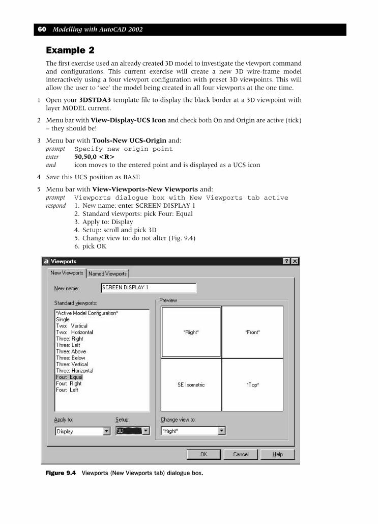
Example 2The first exercise used an already created 3D model to investigate the viewport commandand configurations. This current exercise will create a new 3D wire-frame modelinteractively using a four viewport configuration with preset 3D viewpoints. This willallow the user to ‘see’ the model being created in all four viewports at the one time.
1 Open your 3DSTDA3 template file to display the black border at a 3D viewpoint withlayer MODEL current.
2 Menu bar with View-Display-UCS Icon and check both On and Origin are active (tick)– they should be!
3 Menu bar with Tools-New UCS-Origin and:prompt Specify new origin pointenter 50,50,0 <R>and icon moves to the entered point and is displayed as a UCS icon
4 Save this UCS position as BASE
5 Menu bar with View-Viewports-New Viewports and:prompt Viewports dialogue box with New Viewports tab activerespond 1. New name: enter SCREEN DISPLAY 1
2. Standard viewports: pick Four: Equal3. Apply to: Display4. Setup: scroll and pick 3D5. Change view to: do not alter (Fig. 9.4)6. pick OK
60 Modelling with AutoCAD 2002
Figure 9.4 Viewports (New Viewports tab) dialogue box.
modelling with AutoCAD.qxd 17/06/2002 15:38 Page 60

6 The screen will display a four viewport configuration with the black border displayed ineach. Note the ‘appearance’ of the icon in the top two, and lower right viewports – ithas the same configuration in each, despite the different viewpoints set in the NewViewports dialogue box (respond 4 above)
7 Making each viewport active in turn enter the following:a) at the command line enter UCSVP <R> and:
prompt Enter new value for UCSVP<1>enter 0 <R>
b) at the command line enter ZOOM <R> then 0.9 <R>
8 The screen layout at this stage is similar to Fig. 9.5(a)
9 Note: we will discuss UCSVP in a later chapter
10 With the lower left viewport active, construct the model base using the LINE icon with:Start point 0,0,0 <R> pt1Next point @200,0,0 <R> pt2Next point @0,120,0 <R> pt3Next point @200<180,0 <R> pt4Next point close – fig(b) in 3D
11 Using the LINE command construct the front vertical side with:Start point Intersection icon of pt1Next point @20,0,100 <R> pt5Next point @120,0,0 <R> pt6Next point Intersection icon of pt2Next point right-click/enter – fig(c) in 3D
Tiled viewports 61
Figure 9.5 Construction of model for viewport example 2.
modelling with AutoCAD.qxd 17/06/2002 15:38 Page 61

12 The top surface is created with the LINE command and:Start point Intersection icon of pt6Next point @0,80,0 <R> pt7Next point @–120,0,0 <R> pt8Next point Intersection icon of pt5Next point right-click/enter – fig(d) in 3D
13 Add the sloped sides with lines joining points 3–7 and 4–8 as fig(e) in 3D
14 Make layer OBJECTS (blue) current and draw a circle with centre at 80,40,100 and witha radius of 25 – fig(f) in 3D
15 Menu bar with Draw-Surfaces-3D Surfaces-Box3d and:prompt Specify corner of box and enter: 80,30,0prompt Specify length of box and enter: 50prompt Specify width of box and enter: 40prompt Specify height of box and enter: 30prompt Specify rotation angle of box about Z axis and enter: 20
16 a) Make layer TEXT currentb) Rotate UCS about X axis by 90 and save as FRONTc) Menu bar with Draw-Text-Single Line Text and add the text item AutoCAD,
centred on 80,50 with height 20 and rotation 0
17 a) Set a 3 point UCS on the right sloped surface with:1. origin: midpoint of line 23 – Fig. 9.5(e)2. x axis: intersection of pt 33. y axis: perpendicular to line 674. save UCS as SLOPE
b) Add the single line text item R2002, centred on –5,50 with a height of 15 and arotation angle of 0
18 The complete four viewport configuration display should be similar to Fig. 9.6
19 Save the drawing as MODR2002\TEST3D
20 This completes the two exercises on viewports
21 Notes1. A new system variable was used during this exercise, this being UCSVP. This variable
determines whether the UCS in an active viewport will ‘reflect’ the UCS orientationof that active viewport and:a) UCSVP 0: unlocked, i.e. the UCS will reflect the UCS of the current active viewportb) UCSVP 1: locked, i.e. UCS is independent of the UCS in the current active viewport
2. The default UCSVP value is 1, i.e. locked3. It is recommended that the UCSVP is set to 0, i.e. it always reflects the UCS
position in any active viewport4. The UCSVP must be set in every created viewport
62 Modelling with AutoCAD 2002
modelling with AutoCAD.qxd 17/06/2002 15:38 Page 62

Summary1 Viewports allow multi-screen configurations to be set
2 There are two types of viewport – TILED and UNTILED
3 The viewport type is controlled by the system variable TILEMODE and:a) TILEMODE 1: tiled viewports (fixed)b) TILEMODE 0: untiled viewports (movable) – more later
4 Tiled viewports can have between 1 and 4 ‘divisions’ and ‘fill the screen drawing area’
5 Multi-screen viewports are generally used with the viewpoint command and their fullbenefit will not be appreciated until the various viewpoint options are discussed
6 Multiple viewport layouts are essential to 3D modelling.
Tiled viewports 63
Figure 9.6 Completed viewport example 2 – TEST3D.
modelling with AutoCAD.qxd 17/06/2002 15:38 Page 63

3D views (Viewpoint)3D Views (or viewpoints) determine how the user ‘looks’ at a model and has been usedin previous chapters without any discussion about how it is used. In this chapter we willinvestigate the command in detail using previously created models. When combined withviewports, the user has a very powerful draughting aid – multiple viewports displayingdifferent views of a model.
The viewpoint command has the following selection options:a) Isometric views: SW, SE, NE, NWb) Orthographic views: Top, Bottom, Left, Right, Front, Backc) Plan view: to current UCS, WCS, named UCSd) Viewpoint: with rotate, compass and tripod, vector optionse) Viewpoint Presets: dialogue box selectionf) Real-time 3D rotationg) New Viewports dialogue box
In this chapter we will investigate all of the above selections.
The Viewpoint ROTATE optionThis option requires two angles to be entered by the user:a) the angle in XY plane from the X-axis – the view directionb) the angle from XY plane – the inclination (tilt)
1 Open your MODR2002\3DWFM drawing and:a) erase any dimensions and hatching. b) leave all text items – they will act as a ‘reference’ as the model is viewed from different
angles.
2 Layer MODEL current, UCS BASE and SE Isometric viewpoint
3 Refer to Fig. 10.1 section A
4 At the command line enter VPOINT <R> and:prompt ***Switching to WCS***and Current view directionthen Specify a view point or [Rotate]<display compass and
tripod>enter R <R> – the rotate optionprompt Enter angle in XY plane from X-axisenter 40 <R>prompt Enter angle from XY planeenter 0 <R>prompt ***Returning to UCS***then Regenerating drawingand model displayed as fig(a1), i.e. looking towards the right-rear side from a
horizontal ‘stand-point’ – the view direction.
Chapter 10
modelling with AutoCAD.qxd 17/06/2002 15:38 Page 64
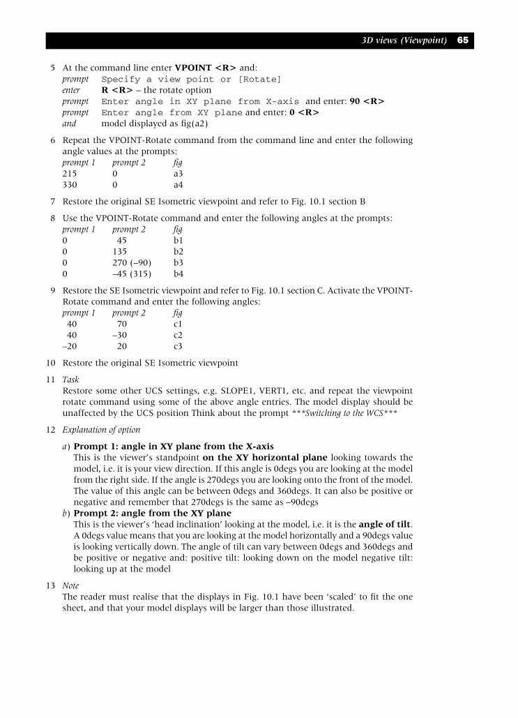
5 At the command line enter VPOINT <R> and:prompt Specify a view point or [Rotate]enter R <R> – the rotate optionprompt Enter angle in XY plane from X-axis and enter: 90 <R>prompt Enter angle from XY plane and enter: 0 <R>and model displayed as fig(a2)
6 Repeat the VPOINT-Rotate command from the command line and enter the followingangle values at the prompts:prompt 1 prompt 2 fig215 0 a3330 0 a4
7 Restore the original SE Isometric viewpoint and refer to Fig. 10.1 section B
8 Use the VPOINT-Rotate command and enter the following angles at the prompts:prompt 1 prompt 2 fig0 45 b10 135 b20 270 (–90) b30 –45 (315) b4
9 Restore the SE Isometric viewpoint and refer to Fig. 10.1 section C. Activate the VPOINT-Rotate command and enter the following angles:prompt 1 prompt 2 fig40 70 c140 –30 c2
–20 20 c3
10 Restore the original SE Isometric viewpoint
11 TaskRestore some other UCS settings, e.g. SLOPE1, VERT1, etc. and repeat the viewpointrotate command using some of the above angle entries. The model display should beunaffected by the UCS position Think about the prompt ***Switching to the WCS***
12 Explanation of option
a) Prompt 1: angle in XY plane from the X-axisThis is the viewer’s standpoint on the XY horizontal plane looking towards themodel, i.e. it is your view direction. If this angle is 0degs you are looking at the modelfrom the right side. If the angle is 270degs you are looking onto the front of the model.The value of this angle can be between 0degs and 360degs. It can also be positive ornegative and remember that 270degs is the same as –90degs
b) Prompt 2: angle from the XY planeThis is the viewer’s ‘head inclination’ looking at the model, i.e. it is the angle of tilt.A 0degs value means that you are looking at the model horizontally and a 90degs valueis looking vertically down. The angle of tilt can vary between 0degs and 360degs andbe positive or negative and: positive tilt: looking down on the model negative tilt:looking up at the model
13 NoteThe reader must realise that the displays in Fig. 10.1 have been ‘scaled’ to fit the onesheet, and that your model displays will be larger than those illustrated.
3D views (Viewpoint) 65
modelling with AutoCAD.qxd 17/06/2002 15:38 Page 65
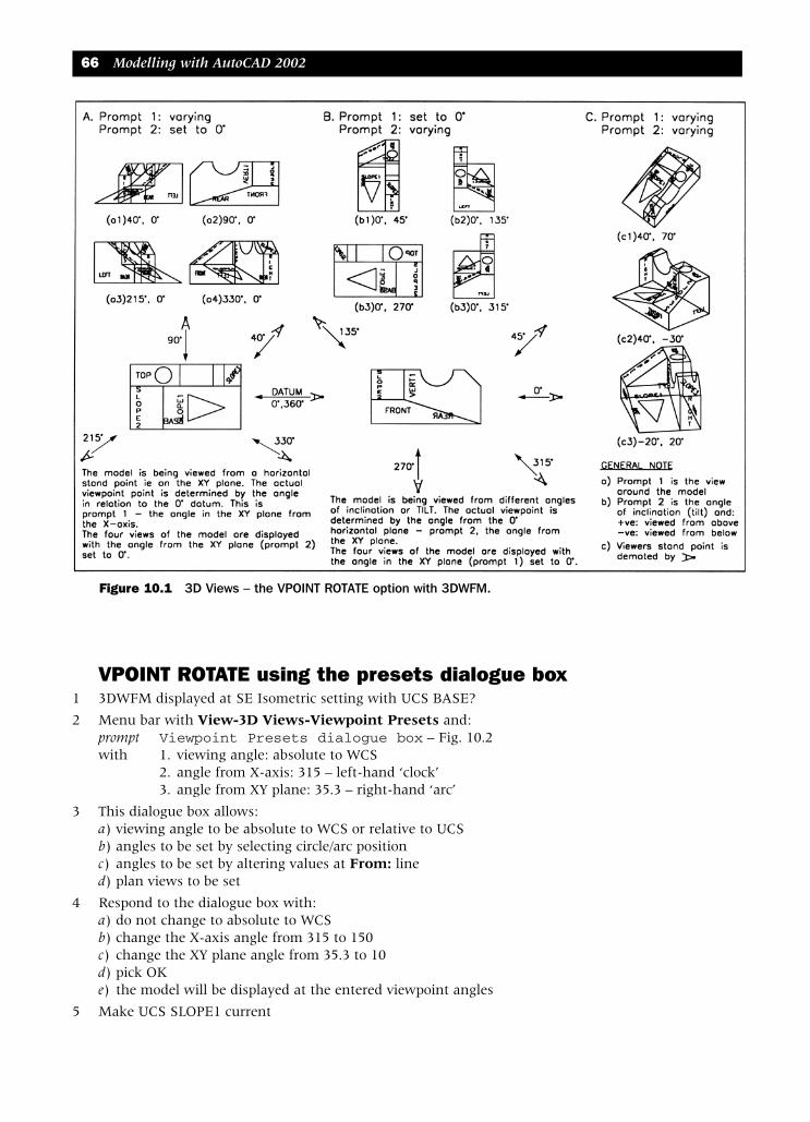
VPOINT ROTATE using the presets dialogue box1 3DWFM displayed at SE Isometric setting with UCS BASE?
2 Menu bar with View-3D Views-Viewpoint Presets and:prompt Viewpoint Presets dialogue box – Fig. 10.2with 1. viewing angle: absolute to WCS
2. angle from X-axis: 315 – left-hand ‘clock’3. angle from XY plane: 35.3 – right-hand ‘arc’
3 This dialogue box allows:a) viewing angle to be absolute to WCS or relative to UCSb) angles to be set by selecting circle/arc positionc) angles to be set by altering values at From: lined) plan views to be set
4 Respond to the dialogue box with:a) do not change to absolute to WCSb) change the X-axis angle from 315 to 150c) change the XY plane angle from 35.3 to 10d) pick OKe) the model will be displayed at the entered viewpoint angles
5 Make UCS SLOPE1 current
66 Modelling with AutoCAD 2002
Figure 10.1 3D Views – the VPOINT ROTATE option with 3DWFM.
modelling with AutoCAD.qxd 17/06/2002 15:38 Page 66

6 Menu bar with View-3D Views-Viewpoint Presets and:a) make Relative to UCS active – black dotb) leave the two angle values as 150 and 10c) pick OKd) the model is displayed at the entered viewpoint angles but differs from the step 4
display due to the UCS setting
7 Taska) Try some other entries from the Viewpoint Presets dialogue box using both selection
methods, i.e. the clock/arc and altering the angles.b) Investigate the difference in the display with the Absolute to WCS and Relative to
UCS selectionsc) Restore Absolute to WCSd) Restore UCS BASE and the SE Isometric viewpoint
8 This completes the viewpoint rotate exercise. Do not save any changes to the 3DWFM model.
3D views (Viewpoint) 67
Figure 10.2 The Viewpoint Presets dialogue box.
modelling with AutoCAD.qxd 17/06/2002 15:38 Page 67
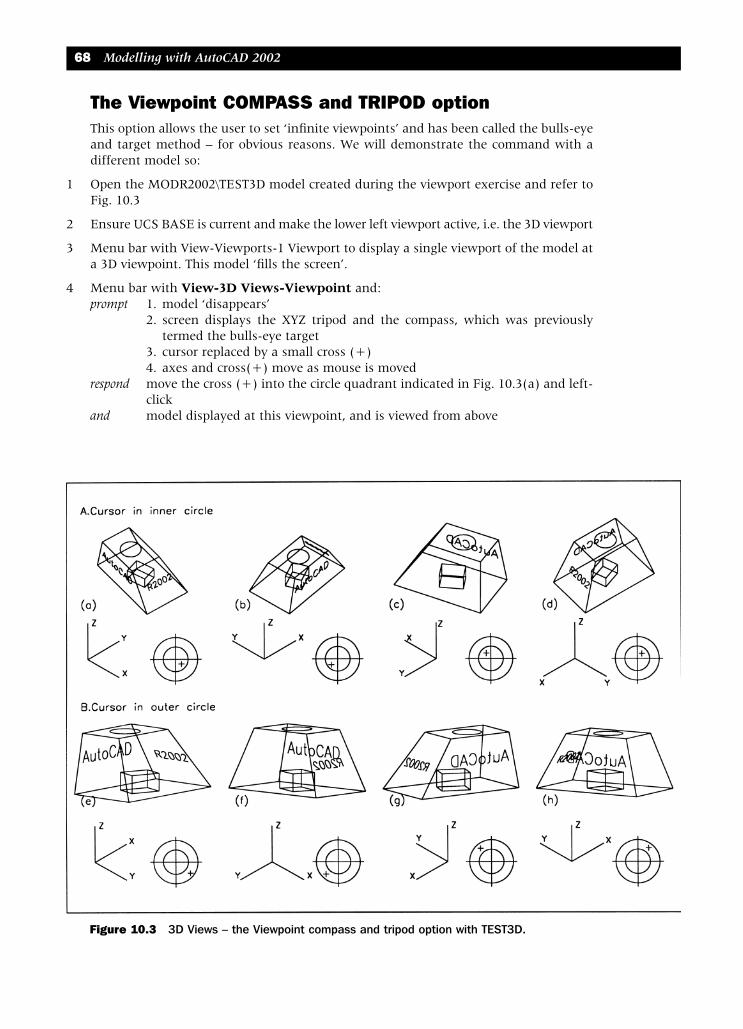
The Viewpoint COMPASS and TRIPOD optionThis option allows the user to set ‘infinite viewpoints’ and has been called the bulls-eyeand target method – for obvious reasons. We will demonstrate the command with adifferent model so:
1 Open the MODR2002\TEST3D model created during the viewport exercise and refer toFig. 10.3
2 Ensure UCS BASE is current and make the lower left viewport active, i.e. the 3D viewport
3 Menu bar with View-Viewports-1 Viewport to display a single viewport of the model ata 3D viewpoint. This model ‘fills the screen’.
4 Menu bar with View-3D Views-Viewpoint and:prompt 1. model ‘disappears’
2. screen displays the XYZ tripod and the compass, which was previouslytermed the bulls-eye target
3. cursor replaced by a small cross (+)4. axes and cross(+) move as mouse is moved
respond move the cross (+) into the circle quadrant indicated in Fig. 10.3(a) and left-click
and model displayed at this viewpoint, and is viewed from above
68 Modelling with AutoCAD 2002
Figure 10.3 3D Views – the Viewpoint compass and tripod option with TEST3D.
modelling with AutoCAD.qxd 17/06/2002 15:38 Page 68

5 At the command line enter VPOINT <R> and:prompt ***Switching to WCS***then Specify a viewpoint or [Rotate]<display compass and tripod>respond press <RETURN>prompt tripod and compass displayedrespond move the cross (+) into the circle quadrant indicated in Fig. 10.3(b) then left-clickand model displayed at this new viewpoint
6 Repeat the tripod viewpoint option (menu bar or command line) and position the cross(+) in the quadrants indicated in Fig. 10.3i.e. (c)–(d): within the inner circle
(e)–(h): between the inner and outer circles
7 TaskWhen you are capable of using the compass and tripod, try the following:a) position the + at different points on the two axes and observe the resultant displaysb) position the + at different points on the circle circumferences and note the displays
8 Explanation of optiona) The ‘bulls-eye’ is in reality a representation of a glassglobe and the model is located
at the centre of the globe. The XY plane is positioned at the equator. The north pole of the globe is at the circle centres and the two concentric circles represent thesurface of the world, stretched out onto a flat plane with: circle centre : the north pole inner circle : the equator outer circle : the south pole
b) As the cross(+) is moved about the circles, the user is moving around the surfacesof the globe and:Cross (+) position View resultin inner circle above equator, looking down on modelin outer circle below equator, looking up at modelon inner circle looking horizontally at modelbelow horizontal viewing from the frontabove horizontal viewing from the rear
9 This completes the tripod option exercise. Do not save changes.
3D views (Viewpoint) 69
modelling with AutoCAD.qxd 17/06/2002 15:38 Page 69

The Viewpoint VECTOR option1 Open MODR2002\3DWFM with UCS BASE and SE Isometric viewpoint.
2 Erase any dimensions and hatching, but leave the text items as they will act as a‘reference’ as the model viewpoint is altered.
3 Refer to Fig. 10.4
4 Menu bar with View-3D Views-Viewpoint and:prompt ***Switching to WCS***then Current view directionand Specify a view point or [Rotate]enter 0,0,1 <R>prompt ***Returning to the UCS***and 1. the model will be displayed at the entered viewpoint
2. it is a top view – fig(a)3. it ‘fills the screen’
6 At the command line enter VPOINT <R> and:prompt Specify a view point or [Rotate]enter 0,–1,0 <R>and model displayed as fig(b) – a front view
70 Modelling with AutoCAD 2002
Figure 10.4 3D Views – the Viewpoint VECTOR option with 3DWFM.
modelling with AutoCAD.qxd 17/06/2002 15:38 Page 70

7 Repeat the viewpoint vector option (menu bar or command line) and enter the followingcoordinates at the prompt line:co-ords view fig1,0,0 from right c0,1,0 from rear d–1,0,0 from left e0,0,–1 from below f1,1,1 3D from above g–1,–1,–1 3D from below h
8 Restore the original SE Isometric viewpoint
9 TaskTry some vector entries for yourself then restore the original SE Isometric viewpoint
10 Explanation of optiona) The vector option allows the user to enter x,y,z coordinates. These are the coordinates
of the viewers ‘stand point’ looking at the model which is considered to be at theorigin. Thus if you enter 0,0,1 you are ‘standing’ at the point 0,0,1 looking towardsthe origin. As this point is on the positive Z axis you are looking down on the model,i.e. a top view.
b) The actual numerical value of the vector entered does not matter, i.e. 0,0,1; 0,0,12;0,0,99.99; 0,0,3456 are all the same viewpoint entries. I prefer to use the number 1,hence 0,0,1; –1,0,0 etc
c) Certain vector entries give the same display as rotate options and the following listssome of these similarities:vector rotate view0,0,1 0,90 top0,–1,0 270,0 front1,0,0 0,0 right0,1,0 90,0 rear–1,0,0 180,0 left0,0,–1 0,–90 bottom1,1,1 45,35 3D from above–1,–1,–1 –135,–35 3D from below
11 This completes the vector option. Do not save any changes.
3D views (Viewpoint) 71
modelling with AutoCAD.qxd 17/06/2002 15:38 Page 71

The Isometric viewpointsThe isometric 3D views allow the user to view a model from four ‘preset’ viewpoints,these being SW, SE, NE and NW. These four viewpoints are used extensively as theyallow easy access to viewing a model in 3D.
1 Open model TEST3D to display the four viewport configuration saved from the previouschapter.
2 Restore UCS BASE with layer MODEL current
3 Making the appropriate viewport active, menu bar with Views-3Dviews and set thefollowing viewpoints:viewport viewpointtop left SW Isometrictop right SE Isometriclower right NE Isometriclower left NW Isometric
4 When the viewpoints have been entered, zoom-all in each viewport and the result shouldbe Fig. 10.5. This does not need to be saved
5 Notes:a) The four preset isometric viewpoints only allow viewing from above. If a model is to
be viewed from below, another option is required. My choice for this is VPOINT-Rotatewith a negative second angle value.
b) The equivalent VPOINT-Rotate angles for the four isometric presets are:3D View angle in XY plane angle from XY planeSW Isometric 225 35.3SE Isometric 315 35.3NE Isometric 45 35.3NW Isometric 135 35.3
72 Modelling with AutoCAD 2002
Figure 10.5 3D Views – the ISOMETRIC Presnts with the TEST3D model.
modelling with AutoCAD.qxd 17/06/2002 15:38 Page 72
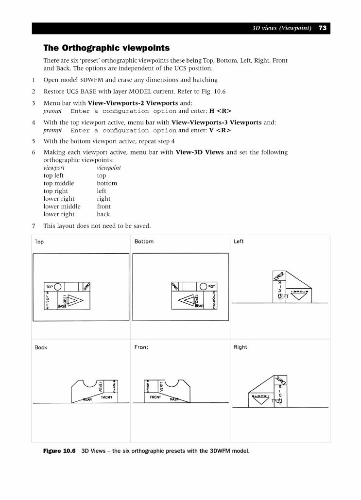
The Orthographic viewpointsThere are six ‘preset’ orthographic viewpoints these being Top, Bottom, Left, Right, Frontand Back. The options are independent of the UCS position.
1 Open model 3DWFM and erase any dimensions and hatching
2 Restore UCS BASE with layer MODEL current. Refer to Fig. 10.6
3 Menu bar with View-Viewports-2 Viewports and:prompt Enter a configuration option and enter: H <R>
4 With the top viewport active, menu bar with View-Viewports-3 Viewports and:prompt Enter a configuration option and enter: V <R>
5 With the bottom viewport active, repeat step 4
6 Making each viewport active, menu bar with View-3D Views and set the followingorthographic viewpoints:viewport viewpointtop left toptop middle bottomtop right leftlower right rightlower middle frontlower right back
7 This layout does not need to be saved.
3D views (Viewpoint) 73
Figure 10.6 3D Views – the six orthographic presets with the 3DWFM model.
modelling with AutoCAD.qxd 17/06/2002 15:38 Page 73

Viewpoint PLAN This viewpoint selection was discussed during the chapter on the UCS and gives a viewperpendicular to a UCS position.
1 Open the four viewport configuration TEST3D and:a) create a single viewport configuration of the 3D viewb) set any 3 viewport configurationc) UCS FRONT current and refer to Fig. 10.7
2 Make any viewport active and menu bar with View-3D Views-Plan View-CurrentUCS and the model will be displayed as fig(a).
3 It is a plan view perpendicular to the UCS FRONT XY plane.
4 With another viewport active, menu bar with View-3D Views-Plan View-World UCSand the model will be displayed as fig(b)
5 Make the third viewport active and select the menu bar sequence View-3D Views-PlanView-Named UCS and:prompt Enter name of UCS and enter: SLOPE <R>
6 The model will be displayed as a view perpendicular to the XY plane of UCS SLOPE.
7 This layout does not need to be saved.
74 Modelling with AutoCAD 2002
Figure 10.7 3D Views – the PLAN options with model TEST3D.
modelling with AutoCAD.qxd 17/06/2002 15:38 Page 74

The VIEW commandDifferent views of a model can be saved within the current drawing, thus allowing theoperator to create a series of ‘pictures’. These could be of the model being constructed,of a completed model at differing viewpoints etc. These views (pictures) can be recalledat any time.
1 Open the 3DWFM model and erase any dimensions and hatching (or freeze theappropriate layers)
2 Model displayed at SE Isometric viewpoint with UCS BASE and layer MODEL current
3 At the command line enter –VIEW <R> and:prompt Enter an option [?/Orthographic/Delete/Restore/Save..enter S <R> – the save optionprompt Enter view name to saveenter V1 <R>
4 Menu bar with View-3D Views and set to NW Isometric
5 Menu bar with View-Named Views and:prompt View dialogue box – Named Views tab activerespond pick Newprompt New View dialogue boxrespond 1. enter View name: V2
2. ensure Current display active, i.e. black dot3. Save UCS with view active (tick)4. UCS name: BASE – Fig. 10.85. pick OK
prompt View dialogue box with V2 added to listrespond pick OK
6 Menu bar with View-3D Views and set to SW Isometric
7 Menu bar with View-Named Views and from the View dialogue box:a) pick Newb) View name: V3 with current display, UCS BASE then OKc) View dialogue box as Fig. 10.9d) pick OK
8 At the command line enter -VIEW <R> and:prompt Enter an optionenter R <R> – the restore optionprompt Enter view name to restore enter V1 <R>and saved view V1 displayed
9 Menu bar with View-Named Views and:prompt View dialogue boxrespond 1. pick V3
2. pick Set Current3. pick OK
and screen displays the saved V3 view
10 Taska) create, save and display some other viewsb) investigate the Details option from the Named Views tabc) investigate the Orthographic & Isometric Views tabd) investigate altering the UCS with saved views
11 When complete, restore the SE Isometric viewpoint. Save if required but not as 3DWFM.
12 NoteDo not confuse the VIEW command with the View option of the UCS command. Theyare two entirely different concepts.
3D views (Viewpoint) 75
modelling with AutoCAD.qxd 17/06/2002 15:38 Page 75

76 Modelling with AutoCAD 2002
Figure 10.10 The Viewports dialogue box (New Viewports tab).
Figure 10.8 The New View dialogue box.
Figure 10.9 The View dialogue box (Named Views tab).
modelling with AutoCAD.qxd 17/06/2002 15:38 Page 76
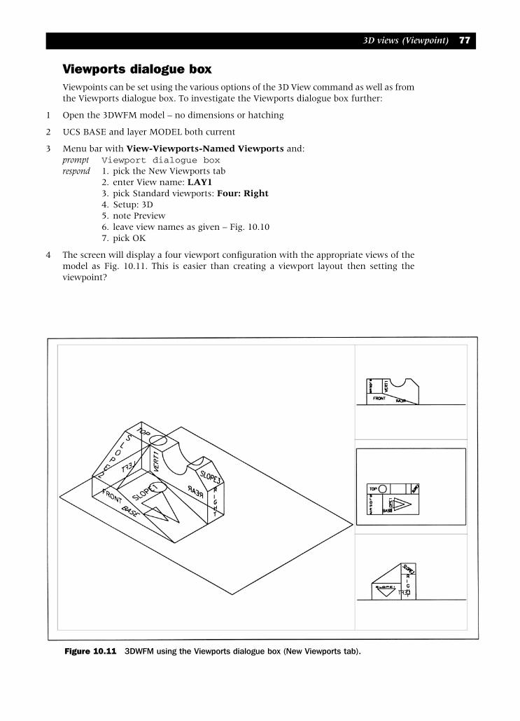
Viewports dialogue boxViewpoints can be set using the various options of the 3D View command as well as fromthe Viewports dialogue box. To investigate the Viewports dialogue box further:
1 Open the 3DWFM model – no dimensions or hatching
2 UCS BASE and layer MODEL both current
3 Menu bar with View-Viewports-Named Viewports and:prompt Viewport dialogue boxrespond 1. pick the New Viewports tab
2. enter View name: LAY13. pick Standard viewports: Four: Right4. Setup: 3D 5. note Preview6. leave view names as given – Fig. 10.107. pick OK
4 The screen will display a four viewport configuration with the appropriate views of themodel as Fig. 10.11. This is easier than creating a viewport layout then setting theviewpoint?
3D views (Viewpoint) 77
Figure 10.11 3DWFM using the Viewports dialogue box (New Viewports tab).
modelling with AutoCAD.qxd 17/06/2002 15:38 Page 77
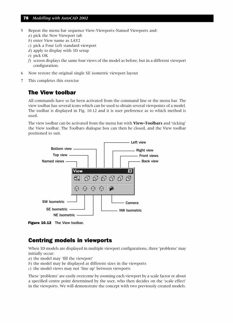
5 Repeat the menu bar sequence View-Viewports-Named Viewports and:a) pick the New Viewport tabb) enter View name as LAY2c) pick a Four Left standard viewportd) apply to display with 3D setupe) pick OKf) screen displays the same four views of the model as before, but in a different viewport
configuration.
6 Now restore the original single SE isometric viewport layout
7 This completes this exercise
The View toolbarAll commands have so far been activated from the command line or the menu bar. Theview toolbar has several icons which can be used to obtain several viewpoints of a model.The toolbar is displayed in Fig. 10.12 and it is user preference as to which method isused.
The view toolbar can be activated from the menu bar with View-Toolbars and ‘ticking’the View toolbar. The Toolbars dialogue box can then be closed, and the View toolbarpositioned to suit.
Centring models in viewportsWhen 3D models are displayed in multiple viewport configurations, three ‘problems’ mayinitially occur:a) the model may ‘fill the viewport’b) the model may be displayed at different sizes in the viewportsc) the model views may not ‘line up’ between viewports
These ‘problems’ are easily overcome by zooming each viewport by a scale factor or abouta specified centre point determined by the user, who then decides on the ‘scale effect’in the viewports. We will demonstrate the concept with two previously created models.
78 Modelling with AutoCAD 2002
Figure 10.12 The View toolbar.
Bottom view
Top view
Named views
SW Isometric
SE Isometric
NE Isometric
Left view
Right viewFront viewsBack view
Camera
NW Isometric
modelling with AutoCAD.qxd 17/06/2002 15:38 Page 78

Example 1 – centring by scale1 Open MODR2002\3DWFM of the wire-frame model and:
a) erase/freeze any dimensions and textb) leave the hatching displayedc) erase the black borderd) Zoom-all and the model ‘fills the screen’e) ensure UCS Icon is on and at origin with menu bar View-Display-UCS Icon (these
should be active)f) ensure UCS BASE is currentg) command line with UCSVP <R> and:
prompt Enter new value for UCSVPrespond enter: 0 <R>
2 Menu bar with View-Viewports-4 Viewports and the model is displayed in 3D in eachviewport
3 By entering VPOINT <R> at the command line, set the following vector viewpoints inthe named active viewports:viewport viewpointtop left 1,0,0top right 0,–1,0lower right 0,0,1lower left 1,–1,1
4 The model will be displayed at the viewpoints entered and will be of differing sizes ineach viewport. The model now needs to be centred about a specific point
5 With the top left viewport active, menu bar with View-Zoom-Scale and:prompt Enter a scale factorrespond enter: 1.75 <R>
6 Repeat the zoom-scale selection in the other three viewports, and enter a scale factor of1.75 in the top right and lower right viewports, but 1 in the lower left (3D) viewport.
7 When the zoom-scale command has been completed, the model will be ‘neatly centred’in all viewports as Fig. 10.13
8 Save as MODR2002\MV3DWFM
3D views (Viewpoint) 79
Figure 10.13 Centre viewport example 1 – 3DWFM by scale factor.
modelling with AutoCAD.qxd 17/06/2002 15:38 Page 79

Example 2 – centring about a user specified point1 Open drawing TEST3D to display the four viewport configuration of the created model
with text on two ‘planes’
2 Erase the black border and zoom-all in each viewport and the model will be displayedat different ‘sizes’ in the viewports
3 Ensure UCS BASE is current
4 a) ensure UCS Icon is on and at originb) in each viewport use the command line UCSVP command and set the variable to 0
5 The model has a basic overall cuboid sizes of 200x120x100 and its ‘centre point’ relative
to UCS BASE is at 100,60,50.
6 With the top left viewport active, menu bar with View-Zoom-Center and:prompt Specify centre point enter 100,60,50 <R>prompt Enter magnification or height <some value>enter 175 <R>
7 Repeat the zoom-center command in the other three viewports and enter the center pointas 100,60,50 and the magnification as 175 but 225 in the 3D viewport
8 The model will be centred in each viewport as Fig. 10.14
9 Save this display as MODR2002\MVTEST3D.
80 Modelling with AutoCAD 2002
Figure 10.14 Centre viewport example 2 – TEST3D by centre/magnification.
modelling with AutoCAD.qxd 17/06/2002 15:38 Page 80

Summary1 The viewpoint command allows models to be viewed from different ‘stand points’
2 The command has several selection options including:a) four preset isometric views – SW, SE, NE and NWb) six orthographic preset views – top bottom, left, right, front and backc) three plan views – current UCS, world UCS, named UCSd) VPOINT with three options – rotate, compass and tripod, vector
3 The VPOINT rotate option requires two angles:a) the angle ‘around’ the model – the directionb) the angle of inclination – the tilt
4 The VPOINT rotate option can be set from a dialogue box
5 The VPOINT compass/tripod option allows unlimited viewpoints
6 The VPOINT vector option requires an x,y,z coordinate entry
7 Viewpoints are generally set absolute to the WCS and the relative to the UCS optionis not recommended
8 All wire-frame models exhibit ambiguity when the viewpoint command is used, i.e.viewed from above or from below?
9 The VIEW command allows different views of a model to be saved in the current drawingfor future recall. This is useful when the model is being displayed at various viewpoints.
10 Models can be centred in multiple tiled viewports using:a) Zoom-scale, the user entering the scale factorb) Zoom-center, the user entering the centre point and the magnification
11 The centre point entered with zoom-center is dependent on the UCS position
12 I like to zoom-centre relative to UCS BASE which is usually ‘set’ at a convenient basevertex. It is then easy for me to work out the model centre point in relation to the overallsize of the model.
13 The magnification value entered is a ‘scale’ effect and is relative to the given default,e.g. if the default is <180> then:a) a value less than 180 will increase the model sizeb) a value greater than 180 will decrease the model size.
3D views (Viewpoint) 81
modelling with AutoCAD.qxd 17/06/2002 15:38 Page 81

AssignmentsTwo activities have been included at this stage, both of which involve creating multipletiled viewports, setting viewpoints and scaling/centring the models. The models havealready been created (hopefully) during the hatching activities.
Activity 8: The hatched shaped block of Macfaramus.
1 Open the drawing of the hatched block from activity 6 and erase the border
2 Create a four viewport configuration to display top, front, right and a 3D view.
3 Zoom-all in each viewport
4 With UCS BASE current, zoom centre about the point 100,60,90 at 225 magnificationin the three orthographic viewports, but 275 in the 3D viewport.
5 When complete, save as MODR2002\MVBLOCK
Activity 9: The hatched pyramid of Macfaramus.
1 Open hatched pyramid model from activity 7 and erase the border
2 Create a four viewport (left) configuration to display top, front, right and a SE Isometricview
3 Either:a) Zoom-scale in each viewport with a scale factor of 1, but with a different scale factor
in the 3D viewportb) with UCS BASE current, zoom centre about the point 100,100,125 at 300
magnification in the three orthogonal viewports and your own entered magnificationin the 3D viewport
4 When complete, save as MODR2002\MVPYR
82 Modelling with AutoCAD 2002
modelling with AutoCAD.qxd 17/06/2002 15:38 Page 82

Model space andpaper space anduntiled viewportsAutoCAD 2002 has multi-view capabilities which allow the user to layout, organise andplot multiple views of any 3D model. The multiple viewport concept has already beenused with our wire-frame models, these viewports being TILED, i.e. fixed.
In this chapter we will investigate how to create UNTILED or FLOATING viewports whichare used in the same way that the tiled viewports were used. The creation of untiledviewports requires an understanding of the two AutoCAD drawing environments – modelspace and paper space.
The model/paper space concepts required by the user are:
1 Model spaceThis is the drawing environment that exists in any viewport and is the default. All modelswhich have been created have been completed in model space. Model space is used forall draughting and design work and for setting 3D viewpoints. Multiple viewports arepossible in model space but are TILED, i.e. they cannot be moved or altered in size – Fig.11.1(a). While model space multi-views are useful, they have one major disadvantage –only the active viewport can be plotted, i.e. model space multiple viewports cannot beplotted on one sheet of paper.
2 Paper spaceThis is a drawing environment which is independent of model space. In paper space theuser creates the drawing sheet, i.e. border, title box, etc. as well as arranging the multipleviewport layout. The viewports created in paper space are UNTILED, i.e. they can bepositioned to suit, altered in size and additional viewports can be added to the layout –Fig. 11.1(b). In paper space the 3D viewpoint command is not valid although objects(particularly text) can be added to the sheet layout. The real advantage of working withpaper space multiple viewports is that any viewport configuration can be plotted on theone sheet of paper.
3 TilemodeThe system variable which controls the ‘type’ of viewport to be created is TILEMODEand:a) TILEMODE 1: model space (FIXED) viewports and paper space is not availableb) TILEMODE 0: paper space (FLOATING) viewports and model space is available
Tiled (model space) viewports are always displayed as edge-to-edge and fill the screenlike a tiled wall. Untiled (paper space) viewports can be positioned anywhere within thescreen area with spaces between them if required. They can also be copied, moved,stretched etc.
4 IconsWhen working in model space the normal WCS/UCS icon will be displayed in allviewports, orientated to the viewport viewpoint as Fig. 11.1(c). In paper space, the paperspace icon – Fig. 11.1(d) is displayed.
Chapter 11
modelling with AutoCAD.qxd 17/06/2002 15:38 Page 83
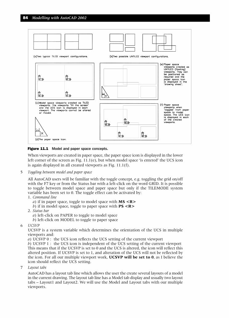
When viewports are created in paper space, the paper space icon is displayed in the lowerleft corner of the screen as Fig. 11.1(e), but when model space ‘is entered’ the UCS iconis again displayed in all created viewports as Fig. 11.1(f).
5 Toggling between model and paper space
All AutoCAD users will be familiar with the toggle concept, e.g. toggling the grid on/offwith the F7 key or from the Status bar with a left-click on the word GRID. It is possibleto toggle between model space and paper space but only if the TILEMODE systemvariable has been set to 0. The toggle effect can be activated by:1. Command line
a) if in paper space, toggle to model space with MS <R>b) if in model space, toggle to paper space with PS <R>
2. Status bara) left-click on PAPER to toggle to model spaceb) left-click on MODEL to toggle to paper space
6 UCSVPUCSVP is a system variable which determines the orientation of the UCS in multipleviewports and:a) UCSVP 0 : the UCS icon reflects the UCS setting of the current viewportb) UCSVP 1 : the UCS icon is independent of the UCS setting of the current viewportThis means that if the UCSVP is set to 0 and the UCS is altered, the icon will reflect thisaltered position. If UCSVP is set to 1, and alteration of the UCS will not be reflected bythe icon. For all our multiple viewport work, UCSVP will be set to 0, as I believe theicon should reflect the UCS setting.
7 Layout tabsAutoCAD has a layout tab line which allows the user the create several layouts of a modelin the current drawing. The layout tab line has a Model tab display and usually two layouttabs – Layout1 and Layout2. We will use the Model and Layout tabs with our multipleviewports.
84 Modelling with AutoCAD 2002
Figure 11.1 Model and paper space concepts.
modelling with AutoCAD.qxd 17/06/2002 15:38 Page 84

Model/paper space example – untiled viewportsThis example will use a model created in model space to demonstrate the paper spacemultiple viewport concept. The example is quite long but if you are unsure of paper space,persevere with it – it is important that you understand how to create and use paper spaceviewports.
Note a) Although you may be familiar with the model/paper space concept it is advisable that
you complete the exercise.b) AutoCAD 2002 assumes that the user has access to a printer or plotter, this being
connected to the computer. As all printer/plotters differ in their configurations, papersize etc, I have assumed that no printer is configured. This does not exclude the userfrom obtaining a hard copy of completed drawings, it is simply a matter ofconvenience for me when detailing the various steps in the exercises.
c) There are different methods of creating paper space untiled viewports from a modelspace drawing. This example demonstrates one of these methods.
1 Open drawing MODR2002\3DWFM and:a) erase the black border, hatching and any dimensionsb) leave the text items – they will ‘act as a reference’c) layer MODEL and UCS BASE currentd) zoom-all and model ‘fills the screen’e) refer to Fig. 11.2
Model space and paper space and untiled viewports 85
Figure 11.2 Creating the paper space multiple viewport layout with 3DWFM.
modelling with AutoCAD.qxd 17/06/2002 15:38 Page 85

2 Make a new layer called VP, linetype continuous, colour 12
3 At the command line enter PS <R> and prompt line will display:
** Command not allowed in Model tab **
4 Menu bar with Tools-Wizards-Create Layout and:prompt Create Layout – Begin dialogue boxrespond enter layout name: MYFIRST then pick Nextprompt Create Layout – Printer dialogue boxrespond pick None then pick Nextprompt Create Layout – Paper Size dialogue boxrespond 1. scroll and pick ISOA3 (420.00x297.00MM)
2. Drawing units: Millimeters3. pick Next
prompt Create Layout – Orientation dialogue boxrespond ensure Landscape active then pick Nextprompt Create Layout – Title Block dialogue boxrespond pick None then pick Nextprompt Create Layout – Define Viewports dialogue boxrespond pick None then pick Nextprompt Create Layout -Finish dialogue boxrespond pick Finishand 1. screen returned in paper space – note the icon
2. the white area is the A3 paper3. the dotted area is the permitted drawing area within the white A3 paper –
for plot purposes4. a new layout name MYFIRST is added to the tab bar
5 Make layer 0 current and menu bar with Draw-Rectangle and:prompt Specify first corner point enter 0,0 <R>prompt Specify other corner point enter 405,257 <R>
6 This rectangle is our drawing area outline
7 Make layer VP current
8 Menu bar with View-Viewports-1 Viewport and:prompt Specify corner of viewport and enter: 10,10 <R>prompt Specify opposite corner and enter: 190,170 <R>and a viewport (A) is created with the model 3DWFM displayed as fig(a)
9 Menu bar with View-Viewports-2 Viewports and:prompt Enter viewport arrangement and enter: V <R>prompt Specify first corner and enter: 10,180 <R>prompt Specify opposite and enter: 215,245 <R>and two additional viewports (B and C) are created, each displaying the model in
3D – fig(b)
10 Menu bar again with View-Viewports-4 Viewports and:prompt Specify first corner and enter: 205,10 <R>prompt Specify opposite corner and enter: 395,150 <R>and four new viewports (D,E,F,G) are created with the model displayed in each – fig(c)
11 Final menu bar selection with View-Viewports-3 Viewports (Right option) and:prompt Specify first corner and enter: 240,170 <R>prompt Specify opposite corner and enter: 440,270 <R>and three viewports (H,I,J) are created each with the model displayed as fig(d).
These viewports extend ‘outwith’ the drawing paper.
86 Modelling with AutoCAD 2002
modelling with AutoCAD.qxd 17/06/2002 15:38 Page 86
12 What has been achieved?a) ten different sized viewports have been createdb) the viewports have been created in paper spacec) each viewport displays the original 3DWFM model
13 At the command line enter MS <R> and:a) toggled to model spaceb) the last viewport (top right) is active?c) each viewport displays the UCS icon at BASE?d) any viewport can be made active as before, i.e. move to required viewport and left-click
14 Investigate the paper/model space toggle:a) from the command line with PS and MSb) status bar with left-click on MODEL/PAPERc) decide on which toggle method you prefer
15 Investigate the model/layout tab line:a) pick Model – the original 3DWFM model is displayedb) pick MYFIRST – our multiple viewport layout is displayed.
16 At this stage the layout is as Fig. 11.2
Setting the viewpoints1 Enter model space and set the following viewpoints in the named viewports:
viewport viewpoint viewport viewpointA SW Isometric F SE IsometricB NE Isometric G TopC NW Isometric H BottomD Right I LeftE Front J Back
2 The model is now displayed at a different viewpoint in each viewport. Using the Zoom-Scale command, enter the following scale factors in the appropriate viewport:a) scale factor of 1.75 in orthogonal view viewportsb) scale factor of 1.25 in 3D view viewports.
3 The UCS icon may not be displayed as expected so:a) in each viewport, enter UCSVP <R> then 0 <R>b) make the largest viewport (A) currentc) restore UCS BASE and the icon should be displayed as expected.
Model space and paper space and untiled viewports 87
modelling with AutoCAD.qxd 17/06/2002 15:38 Page 87

Adding text1 In model space, make layer TEXT current and viewport (A) active
2 Using the menu bar sequence, Draw-Text-Single Line Text, add an item of text usingthe following:a) start point: 0,–30b) height: 15 and rotation: 0c) text item: AutoCAD 2002 (MS)
3 This item of text will be displayed in the ten viewports at different orientations due tothe viewpoints. In some viewports (D,E,I,J) the text is viewed ‘end-on’
4 Enter paper space with PS <R>
5 Menu bar with Draw-Text-Single Line Text and add an item of text using:a) start point: centred on 200,150b) height: 20 and rotation: 0c) text: AutoCAD 2002<R>
text: in <R>text: PAPER SPACE <R><R> – two returns
6 At this stage your screen layout should resemble Fig. 11.3
88 Modelling with AutoCAD 2002
Figure 11.3 Working with the created paper space viewports.
modelling with AutoCAD.qxd 17/06/2002 15:39 Page 88

Modifying the layout1 In paper space try and erase the model – you cannot
2 In model space try and erase the paper space text – not possible
3 In paper space, activate the ZOOM command and window viewport A. The viewport willbe enlarged and by entering model space, it is easier to work on the model.
4 In paper space, zoom previous to restore the original layout
5 In paper space, select the SCALE icon from the Modify toolbar and:prompt Select objectsrespond completely window viewports H,I,J then right-clickprompt Specify base pointrespond Intersection of lower left corner of viewport Jprompt Specify scale factorenter 0.75 <R>
6 In model space:a) zoom-all in viewports H, I and Jb) then zoom-scale with the same 1.75 scale factor as before.
7 Enter paper space and freeze the layer VP
8 The ten views of the model will be displayed with text but without the viewport borders– Fig. 11.4
9 If you have access to a printer/plotter:a) print from any viewport in model spaceb) print from paper space
10 This completes this exercise – save if required.
Model space and paper space and untiled viewports 89
Figure 11.4 Completed paper space exercise with 3DWFM.
modelling with AutoCAD.qxd 17/06/2002 15:39 Page 89

Comparison between model space and paper spaceThe following table gives a brief comparison between the model and paper space drawingenvironments:Model space Paper space
used to create the model used to create the paper layoutmodel can be modified model cannot be modifiedtiled (fixed) viewports untiled (floating) viewportstilemode: 1 tilemode: 0viewports restricted in size viewports to any sizeviewports ‘fill screen’ viewports positioned to suitviewports cannot be altered viewports can be moved, copied etccannot add viewports additional viewports can be createdplot only active viewport all viewports can be plotted3D views active cannot use 3D viewpointWCS or UCS icon paper space iconzoom in active viewport zoom complete viewports
FinallyOne of the major benefits of paper space is the ability to zoom a complete viewport. Thisallows the zoomed viewport to be enlarged, thus allowing the user to ‘see more clearly’the model being created/worked on when in model space. This is a concept with whichthe user should become familiar and the procedure is:
1 Enter paper space with PS <R>
2 Zoom-window a specific viewport, e.g. the 3D viewport
3 Return to model space with MS <R>
4 Complete (or modify) the model
5 Enter paper space with PS <R>
6 Zoom-previous (or All) to restore the complete layout
7 Return to model space with MS <R>
This zoom a viewport in paper space is a very useful concept and will be used in all futureexercises.
90 Modelling with AutoCAD 2002
modelling with AutoCAD.qxd 17/06/2002 15:39 Page 90

New 3D multipleviewport standardsheetNow that the model/paper space concept has been discussed, a new standard sheet willbe created which will allow all future models (surface and solid) to be displayed inmultiple viewports. This standard sheet will be created with three layout tab displays,and the original 3DSTDA3 sheet will be modified as it:a) already has layers, e.g. MODEL, OBJECTS, TEXT, etc.b) has a created dimension style – 3DSTDc) has other variables set
Getting ready1 Close any existing drawings and open your 3DSTDA3 standard sheet – template or
drawing (it does not matter) to display:a) the black border as a SE Isometric viewpointb) the WCS icon at the left vertex of the border
2 Erase the black border – we will not use it again
3 Menu bar with View-Display-UCS Icon and:a) On and Origin active (tick)b) Properties and decide on a 2D or 3D icon display
4 Menu bar with Format-Layer and create two new layers:name colour linetypeVP number 14 continuousSHEET number 212 continuous
5 At the command line enter UCSVP <R> and:prompt Enter new value for UCSVPenter 0 <R>
6 Note the layout tab line – similar to Fig. 12.1(a)
Chapter 12
Figure 12.1 The layout tab displays. (a) Original tab with a 3D icon. (b) The layout tab display after creatingthree new viewport configurations with a 3D icon.
(a) (b)
modelling with AutoCAD.qxd 17/06/2002 15:39 Page 91

The first layout tab display1 Menu bar with Tools-Wizards-Create Layout and with the Create Layout dialogue
box set the following:a) Begin: enter MVLAY1 then Nextb) Printer: None then Nextc) Paper Size: Millimeters, ISO A3 (420×297) then Nextd) Orientation: Landscape then Nexte) Title Block: None then Nextf) Define viewports: None then Nextg) Finish: pick Finish
2 A white paper area will be returned with a dotted drawing area within, this being inpaper space.
3 Make layer SHEET current4 Menu bar with Draw-Rectangle and:
prompt Specify first corner point and enter: 0,0 <R>prompt Specify other corner point and enter: 405,257 <R>
5 Zoom-all and PAN to suit6 Draw a line from: 0,15 to: @405,07 The area at the bottom of the ‘paper’ is for you to ‘customise’ as required. Use layer
SHEET for this.8 Make layer VP current9 Menu bar with View-Viewports-New Viewports and:
prompt New Viewports dialogue boxrespond 1. pick Four: Equal
2. Viewport spacing: 03. Setup: 3D4. Change views to: leave unaltered5. pick OK
prompt Specify first corner and enter: 10,20<R>prompt Specify opposite corner and enter: 395,247<R>
10 The screen will display four paper space viewports within the sheet border11 To set and save some UCS positions, enter model space with the command line entry
MS <R>12 Making each viewport active, enter UCSVP <R> and:
prompt Enter new value for UCSVPenter 0 <R>
13 Make the lower left viewport active then menu bar with Tools-New UCS-World14 Menu bar with Tools-New UCS-Origin and:
prompt Specify new origin point enter 10,10,0 <R>
15 At command line enter UCS <R> then S <R> and:prompt Enter name to save current UCS enter BASE <R>
16 Menu bar with Tools-New UCS-X and:prompt Specify rotation angle about X axisenter 90 <R>
17 Command line with UCS <R> then S <R> and enter: FRONT <R>18 Menu bar with Tools-New UCS-Y and:
prompt Specify rotation angle about Y axis enter 90 <R>
19 Command line with UCS <R> then S <R> and enter: RIGHT <R>20 We have now set and saved three UCS positions – BASE, FRONT and RIGHT. These three
UCS positions will assist with future model creation.21 Restore UCS BASE and make the lower left viewport active
92 Modelling with AutoCAD 2002
modelling with AutoCAD.qxd 17/06/2002 15:39 Page 92

A second layout tab display1 Still with the MVLAY1 tab and the lower left viewport active with UCS BASE current
2 Left-click on the Layout1 tab and:prompt Page Setup – Layout1 tab dialogue boxrespond 1. Plot Device tab active and set:
a) Plotter configuration: None2. Layout Settings tab active and set:
a) Paper size: ISO A3 (420×297)b) Drawing orientation: Landscapec) Plot area: Layoutd) Plot scale: 1:1e) pick OK
and Paper space entered with:a) white drawing paperb) dashed line plotting area c) coloured rectangle – a new viewport
respond erase the viewport
3 Make layer SHEET current
4 Menu bar with Draw-Rectangle and:prompt Specify first corner point and enter: 0,0 <R>prompt Specify other corner point and enter: 405,257 <R>
5 Zoom-all and PAN to suit
6 Draw a line from: 0,15 to: @405,0 and customise the area below this line using layer SHEET
7 Make layer VP current and menu bar with View-Viewports-New Viewports and set:a) Configuration: Two verticalb) Spacing: 0c) Setup: 3Dd) Change view to: leave at presente) first corner: 10,20f) opposite corner: 395,247
8 Enter model space and:a) set UCSVP to 0 in each viewportb) restore UCS BASE
9 Make the right viewport active and with VPOINT <R> at the command line:a) enter R <R> for the rotate optionb) enter 210 as the angle in the XY planec) enter 30 as the angle from the XY plane
10 With the left viewport active, VPOINT <R> again and:a) enter R <R> for the rotate optionb) enter 210 as the angle in the XY planec) enter –30 as the angle from the XY plane
11 We have set two viewpoints in this layout tab, one from above (the right viewport) andone from below (the left)
12 Right-click on Layout1 tab name and:prompt Shortcut menurespond pick Renameprompt Rename Layout dialogue boxrespond 1. alter name to MVLAY2
2. pick OK
13 Now have created two layout settings, MVLAY1 and MVLAY2 with the Model tab stillavailable.
New 3D multiple viewport standard sheet 93
modelling with AutoCAD.qxd 17/06/2002 15:39 Page 93
A third layout tab displayAlthough we have created two layout tab displays, we will create a third layout tabconfiguration which is slightly different from the two ‘traditional’ layouts MVLAY1 andMVLAY2. The sequence is long and uses coordinates for most of the entries. I would askthe user to persevere with this exercise, as the end result is worth the time and effortspent.
1 Still with the MVLAY2 tab and the right viewport active with UCS BASE current
2 Left-click on the Layout2 tab and:prompt Page Setup – Layout2 tab dialogue boxrespond 1. Plot Device tab active and set:
a) Plotter configuration: None2. Layout Settings tab active and set:
a) Paper size: ISO A3 (420x297)b) Drawing orientation: Landscapec) Plot area: Layoutd) Plot scale: 1:1e) pick OK
and Paper space entered with:a) white drawing paperb) dashed line plotting area c) coloured rectangle – a new viewport
respond erase the viewport
3 Make layer SHEET current
4 Menu bar with Draw-Rectangle and:prompt Specify first corner point and enter: 0,0 <R>prompt Specify other corner point and enter: 405,257 <R>
5 Zoom-all and PAN to suit
6 Draw a line from: 0,15 to: @405,0 and customise the area below this line using layerSHEET
7 Make layer VP current
8 Menu bar with View-Viewports-Polygonal Viewport and:prompt Specify start point and enter: 5,140 <R>prompt Specify next point and enter: 140,140 <R>prompt Specify next point and enter: 170,195 <R>prompt Specify next point and enter: 170,250 <R>prompt Specify next point and enter: 5,250 <R>prompt Specify next point and enter: C <R> – the close option
9 A five sided viewport will be displayed at the top left corner of the drawing area
10 Menu bar with Modify-Mirror and:prompt Select objectsrespond pick any point on viewport then right-clickprompt First point of mirror line and enter: 202.5,15 <R>prompt Second point of mirror line and enter: 202.5,250 <R>prompt Delete source objects and enter: N <R>
94 Modelling with AutoCAD 2002
modelling with AutoCAD.qxd 17/06/2002 15:39 Page 94

11 Repeat the menu bar with Modify-Mirror selection and:prompt Select objectsrespond pick any point on the two viewports then right-clickprompt First point of mirror line and enter: 0,136 <R>prompt Second point of mirror line and enter: 405,136 <R>prompt Delete source objects and enter: N <R>
12 We have now created four polygonal viewports
13 Menu bar with View-Viewports-Polygonal Viewport and:prompt Specify start point and enter: 152.5,136 <R>prompt Specify next point or [Arc/Length/Undo]enter A <R> the arc optionprompt Enter arc boundary optionenter CE <R> – the centre point optionprompt Specify center point of arc and enter: 202.5,136 <R>prompt Specify endpoint of arc and enter: 252.5,136 <R>prompt Specify endpoint of arc and enter: 152.5,136 <R>prompt Specify endpoint of arc and <RETURN> to end command
14 We have now added a circular viewport to our Layout3 display
15 Enter model space and make any of the new viewports active
16 Menu bar with View-Display-UCS Icon and ensure that On and Origin are both active.I had to complete this sequence in all the five viewports
17 Enter UCSVP and 0 in all viewports
18 Make layer MODEL current and restore UCS BASE
19 Set five viewpoints to your own specification. I set the viewpoints to SE Isometric, Left,Right, Front and Top, but it is your choice
20 Right-click on Layout2 tab and:a) pick Rename from shortcut menub) enter MVLAY3 as the layout namec) pick OK
21 At this stage the layout tab should display Model, MVLAY1, MVLAY2 and MVLAY3similar to Fig. 12.1(b)
22 If the layout tab names are ‘not in order’ then right-click an MVLAY name and use theMove/Copy option of the shortcut menu to position as required.
New 3D multiple viewport standard sheet 95
modelling with AutoCAD.qxd 17/06/2002 15:39 Page 95

Saving the layouts as a new standard sheet1 Make any layout tab MVLAY1 (for example) current
2 Enter model space with the lower left viewport active
3 Layer MODEL and UCS BASE current
4 Menu bar with File-Save As and:prompt Save Drawing As dialogue boxrespond 1. scroll at Files of Type
2. pick AutoCAD Drawing Template File (*.dwt)prompt list of existing template files in the AutoCAD template folderrespond 1. enter File name as: MV3DSTD
2. Measurement: Metric3. pick Save
prompt Template Description dialogue boxrespond 1. enter: My multi-view 3D prototype layout drawing created on
XX/YY/ZZ2. pick OK
5 Repeat step 2, but save as a template to your named folder with the same name, i.e.MV3DSTD
6 Menu bar with File-Save As and:prompt Save Drawing As dialogue boxrespond 1. scroll and pick AutoCAD 2000 Drawing (*.dwg)
2. scroll and pick your named folder (MODR2002)3. enter file name: MV3DSTD4. pick Save
7 The template/drawing file will be used extensively when starting new model exercises.
Checking the new MV3DSTD layoutNow that the MV3DSTD template file has been created we will add some 3D objects to‘check’ the layout. Try and reason out the coordinate entries.
1 Close any existing drawings
2 Menu bar with File-New and:prompt Create New Drawing dialogue boxrespond 1. pick Use a Template
2. scroll and pick MV3DSTD.dwt – Fig. 12.23. pick OK
96 Modelling with AutoCAD 2002
Figure 12.2 The Use a Template dialogue box with MV3DSTD selected.
modelling with AutoCAD.qxd 17/06/2002 15:39 Page 96

3 The created multiple viewport drawing should be displayed with the layout tab currentthat you saved as.
4 Display the Object Snap and Surfaces toolbars
5 Menu bar with Draw-Surfaces-3D Surfaces and:prompt 3D Objects dialogue boxrespond pick Box3d then OKprompt Specify corner of box and enter: 0,0,0 <R>prompt Specify length of box and enter: 200 <R>prompt Specify width of box and enter: 100 <R>prompt Specify height and enter: 80 <R>prompt Specify rotation angle about Z axis and enter: 0 <R>
6 Menu bar with Draw-Surfaces-3D Surfaces and:prompt 3D Objects dialogue boxrespond pick Wedge then OKprompt Specify corner point of wedge and enter: 0,0,0 <R>prompt Specify length of wedge and enter: 100 <R>prompt Specify width of wedge and enter: 100 <R>prompt Specify height of wedge and enter: 100 <R>prompt Specify rotation angle of wedge about Z axis and enter: –90 <R>
7 At the command line enter CHANGE <R> and:prompt Select objectsrespond pick the wedge then right-clickprompt Specify change point or [Properties] and enter: P <R>prompt Enter property to change and enter: C <R>prompt Enter new color and enter: BLUE <R><R> – two returns
8 Select the CONE icon from the Surfaces toolbar and:prompt Specify center point for base of cone and enter: 70,50,80 <R>prompt Specify radius for base of cone and enter: 50 <R>prompt Specify radius for top of cone and enter: 0 <R>prompt Specify height of cone and enter: 100 <R>prompt Enter number of segments for surface of cone and enter: 16 <R>
9 Change the colour of the cone to green
10 Select the DISH icon from the Surface toolbar and:prompt Specify center point of dish and enter: 150,50,0 <R>prompt Specify radius of dish and enter: 50 <R>prompt Enter number of longitudinal segments for surface of dishand – enter: 16<R>prompt Enter number of latitudinal segments for surface of dishand – enter: 8 <R>
11 Change the colour of the dish to magenta
12 Make each viewport current and:a) zoom to extentsb) zoom to a scale of 1
13 With UCS BASE make layer TEXT current and menu bar with Draw-Text-Single LineText and:prompt Specify start point of text and enter: 130,80,80 <R>prompt Specify height and enter: 10 <R>prompt Specify rotation angle of text and enter: 0 <R>prompt Text and enter: AutoCAD <R><R>
New 3D multiple viewport standard sheet 97
modelling with AutoCAD.qxd 17/06/2002 15:39 Page 97

14 Add two other text items using the following information:first item second item
Named UCS FRONT RIGHTstart point 110,40,0 15,15,200height 15 20rotation 0 0item Release 2002
15 Restore UCS BASE
16 Enter paper space with PS <R>
17 At the command line enter DTEXT <R> and add the following text using theinformation given:a) start point: centred on 202.5,133.5b) height: 10 and rotation: 0c) enter text: AutoCAD <R>
enter text: 2002 <R>enter text: Paper space <R><R>
18 Return to model space with MS <R>
19 Menu bar with View-Hide in each viewport and your model will be displayed withhidden line removal – Fig. 12.3(a)
20 Now select the MVLAY2 tab and:a) in each viewport Zoom-Extentsb) Zoom-Scale with a 1 scale factorc) hide each viewport – Fig. 12.3(b)
98 Modelling with AutoCAD 2002
Figure 12.3 The layout tabs for checking the MV3DSTD standard sheet.
modelling with AutoCAD.qxd 17/06/2002 15:39 Page 98

21 Select the MVLAY3 tab and repeat the three entries (a), (b) and (c) as step 20 – Fig. 12.3(c)
22 Select the Model tab to display the original 3D view of the model and hide – Fig. 12.3(d)
23 Taska) Using each tab name and in model space, make each viewport active and menu bar
with View-Shade-Gouraud Shaded to display the model in colour. Note the effectof the shading on the model space and paper space text.
b) When you have completed shading, menu bar with View-Shade-2D Wireframe torestore the original views of the model. This will also restore the paper space text –interesting?
This (long) chapter is now complete. You do not have to save the drawing, but if you dobe careful not to over-write your standard sheet.
We can concentrate on surface and solid modelling.
New 3D multiple viewport standard sheet 99
modelling with AutoCAD.qxd 17/06/2002 15:39 Page 99
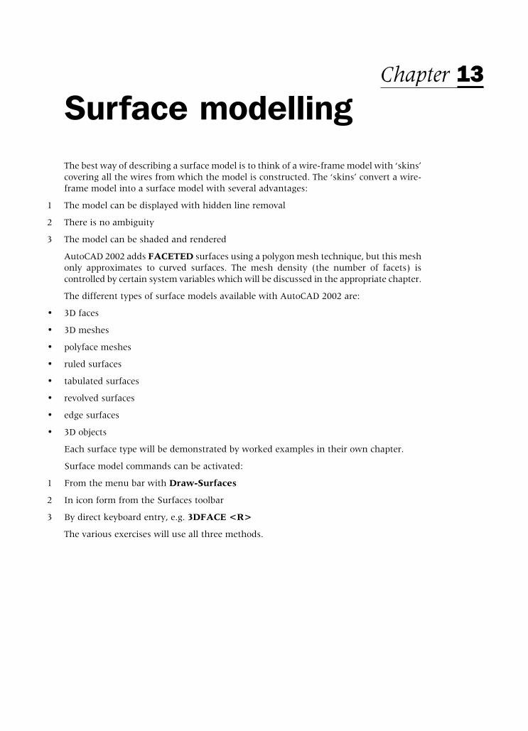
Surface modellingThe best way of describing a surface model is to think of a wire-frame model with ‘skins’covering all the wires from which the model is constructed. The ‘skins’ convert a wire-frame model into a surface model with several advantages:
1 The model can be displayed with hidden line removal
2 There is no ambiguity
3 The model can be shaded and rendered
AutoCAD 2002 adds FACETED surfaces using a polygon mesh technique, but this meshonly approximates to curved surfaces. The mesh density (the number of facets) iscontrolled by certain system variables which will be discussed in the appropriate chapter.
The different types of surface models available with AutoCAD 2002 are:
• 3D faces
• 3D meshes
• polyface meshes
• ruled surfaces
• tabulated surfaces
• revolved surfaces
• edge surfaces
• 3D objects
Each surface type will be demonstrated by worked examples in their own chapter.
Surface model commands can be activated:
1 From the menu bar with Draw-Surfaces
2 In icon form from the Surfaces toolbar
3 By direct keyboard entry, e.g. 3DFACE <R>
The various exercises will use all three methods.
Chapter 13
modelling with AutoCAD.qxd 17/06/2002 15:39 Page 100

3DFACE and PFACEThese two commands appear similar in operation, both adding faces (skins) to wire-framemodels. If these added faces are in colour, the final model display can be quite impressive.
3Dface example 1A 3Dface is a three or four sided surface added to an object and is independentof the UCS position.
1 Close any existing drawings then menu bar with File-New and ‘open’ your MV3DSTDtemplate file with layer MODEL and UCS BASE both current
2 Ensure MVLAY1 tab is current and:a) display toolbars to suitb) make the lower left (3D) viewport activec) zoom-centre about the point 60,35,50 at 175 magnification
3 Create a wire-frame model using the LINE command and the reference sizes in Fig. 14(a)Ensure that point 1 is (0,0,0)
4 When the 3D wire-frame model is complete:a) make each of the other viewports active and zoom-extents then zoom to a factor of
2 in eachb) make the 3D viewport active
5 The created model has five ‘planes’ so make five new layers: F1 red, F2 blue, F3 green,F4 magenta and F5 colour 14.
6 Make layer F1 current
7 Still with the 3D viewport active, menu bar with Draw-Surfaces-3Dface and:prompt Specify first pointrespond Intersection icon and pick pt1prompt Specify second point respond Intersection icon and pick pt2prompt Specify third point respond Intersection icon and pick pt3prompt Specify fourth pointrespond Intersection icon and pt4prompt Specify third pointrespond right-click/enter
8 Make layer F2 current and select the 3DFACE icon from the Surfaces toolbar and:prompt Specify first point and pick Intersection pt2prompt Specify second point and pick Intersection pt3prompt Specify third point and pick Intersection pt5prompt Specify fourth point and pick Intersection pt2 then <R>
9 Make layer F3 current, enter 3DFACE <R> at the command line and:prompt First point and pick Intersection pt3prompt Second point and pick Intersection pt4prompt Third point and pick Intersection pt6prompt Fourth point and pick Intersection pt5 then <R>
Chapter 14
modelling with AutoCAD.qxd 17/06/2002 15:39 Page 101
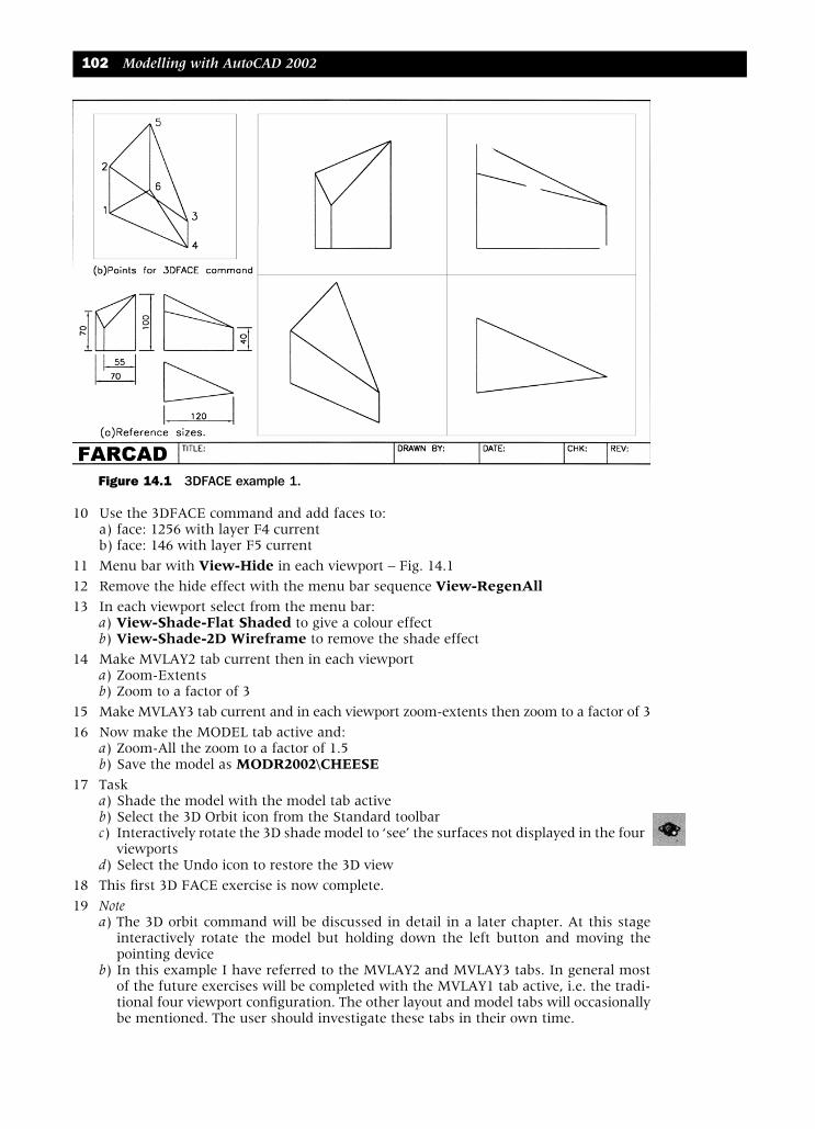
10 Use the 3DFACE command and add faces to:a) face: 1256 with layer F4 currentb) face: 146 with layer F5 current
11 Menu bar with View-Hide in each viewport – Fig. 14.112 Remove the hide effect with the menu bar sequence View-RegenAll13 In each viewport select from the menu bar:
a) View-Shade-Flat Shaded to give a colour effectb) View-Shade-2D Wireframe to remove the shade effect
14 Make MVLAY2 tab current then in each viewporta) Zoom-Extentsb) Zoom to a factor of 3
15 Make MVLAY3 tab current and in each viewport zoom-extents then zoom to a factor of 316 Now make the MODEL tab active and:
a) Zoom-All the zoom to a factor of 1.5b) Save the model as MODR2002\CHEESE
17 Taska) Shade the model with the model tab activeb) Select the 3D Orbit icon from the Standard toolbarc) Interactively rotate the 3D shade model to ‘see’ the surfaces not displayed in the four
viewportsd) Select the Undo icon to restore the 3D view
18 This first 3D FACE exercise is now complete.19 Note
a) The 3D orbit command will be discussed in detail in a later chapter. At this stageinteractively rotate the model but holding down the left button and moving thepointing device
b) In this example I have referred to the MVLAY2 and MVLAY3 tabs. In general mostof the future exercises will be completed with the MVLAY1 tab active, i.e. the tradi-tional four viewport configuration. The other layout and model tabs will occasionallybe mentioned. The user should investigate these tabs in their own time.
102 Modelling with AutoCAD 2002
Figure 14.1 3DFACE example 1.
modelling with AutoCAD.qxd 17/06/2002 15:39 Page 102

3D Face example 2The 3DFACE command can be used to face any three or four sided ‘plane’. The commandallows ‘continuous’ faces to be created and will be demonstrated with a 2D example(although the procedure is valid in 3D) so:
1 With the MODEL tab active:a) erase the model (saved?)b) restore a plan view with the menu bar sequence View-3D Views-Plan View-
Current UCSc) set the snap to 5 and the grid to 10d) zoom-all and refer to Fig. 14.2
2 Activate the 3DFACE command and:prompt Specify first point or [Invisible] respond pick any pt1 on the screenprompt Specify second point or [Invisible] respond pick any pt2 on the screenprompt Specify third point or [Invisible[<exit> respond pick any pt3 (which is the 1st pt of the next face)prompt Specify fourth point or [Invisible]<create three-sided face>respond pick any pt4 (which is the 2nd pt of the next face)and Face 1–2–3–4 displayedprompt Specify third point respond pick any pt5 (3rd pt of face and 1st pt of next face)prompt Specify fourth point respond pick any pt6 (4th pt of face and 2nd pt of next face)and Face 3–4–5–6 displayedprompt Specify third point respond pick any pt7 (3rd pt of face and 1st pt of next face)prompt Specify fourth point respond pick any pt8 (4th pt of face and 2nd pt of next face)and Face 5–6–7–8 displayedprompt Specify third point..respond in response to the third and fourth point prompts:
a) pick any points 9 and 10b) then pick any points 11 and 12c) then pick any points 13 and 14 in responsed) then right-click/enter
and Faces 7–8–9–10; 9–10–11–12; 11–12–13–14 will be displayed as fig(a)
3 Activate the 3DFACE command again and:prompt Specify first point and pick any ptaprompt Specify second point and pick any ptbprompt Specify third point and pick any ptc (1st of next face)prompt Specify fourth point and press <RETURN> – note the promptand Face a-b-c displayedprompt Specify third point and pick any ptd (2nd pt of face)prompt Specify fourth point and pick any pte (3rd pt of face)and Face c-d-e displayedprompt Specify third point and pick any ptfprompt Specify fourth point and <R><R> – two returnsand Face d-e-f displayed as fig(b)
4 Now erase the two continuous 3D faces.
3DFACE and PFACE 103
modelling with AutoCAD.qxd 17/06/2002 15:39 Page 103

The invisible edge (3D Face example 3)When the 3DFACE command is used with continuous three/four-sided ‘shapes’, allthree/four sides of the face are displayed. It is possible to create a 3DFACE with an‘invisible edge’ which will be demonstrated with the following example.
1 Refer to Fig. 14.2(c) and with the Model tab still active:a) make MVLAY1 tab activeb) enter model spacec) layer MODEL and UCS BASE currentd) toggle the grid and snap off
2 Change the viewpoint in the following viewports:a) lower left: VPOINT ‘Rotate’ at 300degs and 30degsb) upper left: VPOINT ‘Rotate’ at 30degs and 30 degsc) upper right and lower right: your own VPOINT ‘Rotate’ values
3 Set the running object snap to INTERSECTION
4 Create a 3D wire-frame model using the sizes given. This should be easy for you (?) butuse your discretion if unsure of sizes
5 With layer F1 current, 3DFACE the four vertical sides of the lower part of the model
6 With layer F3 current, 3DFACE the four vertical sides of the upper part of the model
7 With layer F4 current, 3DFACE the top of the model
104 Modelling with AutoCAD 2002
Figure 14.2 Continuous 3DFACE example.
modelling with AutoCAD.qxd 17/06/2002 15:39 Page 104

8 With layer F2 current:a) activate the 3DFACE command and:
prompt Specify first point and pick pt1prompt Specify second point and pick pt2prompt Specify third point and pick pt3prompt Specify fourth point and pick pt4 the right-click/enter
b) activate the 3DFACE command and:prompt Specify first point and pick pt1prompt Specify second point and pick pt6prompt Specify third point and pick pt5prompt Specify fourth point and pick pt4 then right-click/enter
9 Menu bar with View-Hide and the model will be displayed with hidden line removal.The edge between point 1 and 4 is visible as displayed in fig(d)
10 Menu bar with View-Shade-Flat Shaded and the model is displayed with coloured3D faces. No edge is visible between points 1 and 4 due to the two added faces havingthe same colour
11 Restore the original wire-frame model with the menu bar sequence View-Shade-2DWireframe
12 Erase the two blue 3D face surfaces by picking the edges between points 1 and 4
13 Still with layer F2 current and running object snap set:a) activate the 3DFACE command and:
prompt Specify first point and pick pt1prompt Specify second point and pick pt2prompt Specify third point and pick pt3prompt Specify fourth pointenter I <R> – the invisible edge optionprompt Specify fourth point and pick pt4prompt Specify third point and right-click/enterand the 3D face is displayed without edge 1–4
b) 3DFACE again and:prompt Specify first point and pick pt1prompt Specify second point and pick pt6prompt Specify third point and pick pt5prompt Specify fourth point and enter: I <R>prompt Specify fourth point pick pt4prompt Specify third point and right-click/enterand the 3D face is displayed without edge 1–4
14 Display the model with hidden line removal – fig(e)
15 Try some different shade effects then restore the original wire- frame model
16 Cancel the object snap intersection mode.
17 Save if required, but it will not be used again.
3DFACE and PFACE 105
modelling with AutoCAD.qxd 17/06/2002 15:39 Page 105
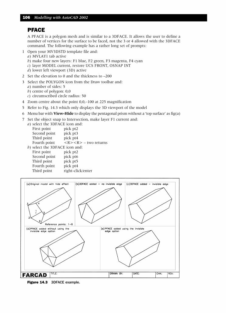
PFACEA PFACE is a polygon mesh and is similar to a 3DFACE. It allows the user to define anumber of vertices for the surface to be faced, not the 3 or 4 allowed with the 3DFACEcommand. The following example has a rather long set of prompts:
1 Open your MV3DSTD template file and:a) MVLAY1 tab activeb) make four new layers: F1 blue, F2 green, F3 magenta, F4 cyanc) layer MODEL current, restore UCS FRONT, OSNAP INTd) lower left viewport (3D) active
2 Set the elevation to 0 and the thickness to –200
3 Select the POLYGON icon from the Draw toolbar and:a) number of sides: 5b) centre of polygon: 0,0c) circumscribed circle radius: 50
4 Zoom centre about the point 0,0,–100 at 225 magnification
5 Refer to Fig. 14.3 which only displays the 3D viewport of the model
6 Menu bar with View-Hide to display the pentagonal prism without a ‘top surface’ as fig(a)
7 Set the object snap to Intersection, make layer F1 current and:a) select the 3DFACE icon and:
First point pick pt2Second point pick pt3Third point pick pt4Fourth point <R><R> – two returns
b) select the 3DFACE icon and:First point pick pt2Second point pick pt6Third point pick pt5Fourth point pick pt4Third point right-click/enter
106 Modelling with AutoCAD 2002
Figure 14.3 3DFACE example.
modelling with AutoCAD.qxd 17/06/2002 15:39 Page 106

8 Hide the model to display the ‘top surface’ as fig(b) i.e. with hidden line removal. Restorethe original wire-model from the menu bar with View-Regen
9 Make layer F2 current and freeze layer F1 then:a) activate the 3DFACE command and:
First point pick pt2Second point pick pt3Third point enter I <R> then pick pt4Fourth point <R><R> – two returns
b) 3DFACE again and:First point pick pt2
Second point pick pt6Third point pick pt5Fourth point enter I <R> then pick pt4Third point right-click/enter
10 Hide to display the model with the 3D face invisible edge option as fig(c)
11 Make layer F3 current and freeze layer F2
12 At the command line enter PFACE <R> and:prompt Specify location for vertex 1 and enter: 0,0 <R> i.e. pt1prompt Specify location for vertex 2 and pick pt2prompt Specify location for vertex 3 and pick pt3prompt Specify location for vertex 4 and pick pt4prompt Specify location for vertex 5 and pick pt5prompt Specify location for vertex 6 and pick pt6prompt Specify location for vertex 7 and right-click: no more verticesprompt Face 1,vertex 1then Enter a vertex number and enter1 <R>and Enter the following in response to the vertex number
prompts:prompt Face 1,vertex 2 and enter: 2 <R>prompt Face 1,vertex 3 and enter: 3 <R>prompt Face 1,vertex 4 and <RETURN> i.e. end of face 1prompt Face 2, vertex 1 and enter: 1prompt Face 2, vertex 2 and enter: 3prompt Face 2, vertex 3 and enter: 4prompt Face 2, vertex 4 and <RETURN> i.e. end of face 2prompt Face 3, vertex 1 and enter: 1prompt Face 3, vertex 2 and enter: 4prompt Face 3, vertex 3 and enter: 5prompt Face 3, vertex 4 and <RETURN> i.e. end of face 3prompt Face 4, vertex 1 and enter: 1prompt Face 4, vertex 2 and enter: 5prompt Face 4, vertex 3 and enter: 6prompt Face 4, vertex 4 and <RETURN> i.e. end of face 4prompt Face 5, vertex 1 and enter: 1prompt Face 5, vertex 2 and enter: 6prompt Face 5, vertex 3 and enter: 2prompt Face 5, vertex 4 and <RETURN> i.e. end of face 5prompt Face 6, vertex 1 and <RETURN> to end command.
13 Menu bar with View-Hide to display the end of the prism with a PFACE surface – fig(d)
14 Make layer F4 current and freeze layer F3
3DFACE and PFACE 107
modelling with AutoCAD.qxd 17/06/2002 15:39 Page 107

15 Repeat the PFACE command line entry and:prompt Specify location for vertex 1 and enter: 0,0 <R>prompt Specify location for vertex 2 and pick pt2prompt Specify location for vertex 3 and pick pt3prompt Specify location for vertex 4 and pick pt4prompt Specify location for vertex 5 and pick pt5prompt Specify location for vertex 6 and pick pt6prompt Specify location for vertex 7 and <RETURN>prompt Face 1, vertex 1, Enter a vertex number and enter: –1 <R>prompt Face 1, vertex 2 and enter: 2 <R>prompt Face 1, vertex 3 and enter: –3 <R>prompt Face 1, vertex 4 and <RETURN>prompt Face 2, vertex 1 and enter: –1prompt Face 2, vertex 2 and enter: 3prompt Face 2, vertex 3 and enter: –4prompt Face 2, vertex 4 and <RETURN>prompt Face 3, vertex 1 and enter: –1prompt Face 3, vertex 2 and enter: 4prompt Face 3, vertex 3 and enter: –5prompt Face 3, vertex 4 and <RETURN>prompt Face 4, vertex 1 and enter: –1prompt Face 4, vertex 2 and enter: 5prompt Face 4, vertex 3 and enter: –6prompt Face 4, vertex 4 and <RETURN>prompt Face 5, vertex 1 and enter: –1prompt Face 5, vertex 2 and enter: 6prompt Face 5, vertex 3 and enter: –2prompt Face 5, vertex 4 and <RETURN>prompt Face 6, vertex 1 and <RETURN>
16 Now View-Hide to display the model with the hidden edge option of the PFACEcommand.
17 The negative (–1, etc.) entry for the face/vertex prompt is the invisible edge option. Thinkthis out for the vertices being entered
18 Save if required, but this model will not be used again.
108 Modelling with AutoCAD 2002
modelling with AutoCAD.qxd 17/06/2002 15:39 Page 108

Summary1 The 3DFACE and PFACE commands allow surface models to be created by drawing
‘skins’ over wire-frame models
2 The HIDE command allows surface models to be displayed with hidden line removal
3 The 3DFACE command can only be used with three or four sided ‘shapes’ althoughcontinuous faces can be created
4 The PFACE command can be used with multi-sided figures
5 Both commands have an invisible edge option
6 The commands can be activated:a) 3DFACE: command line, menu bar or iconb) PFACE: command line only
7 Using separate coloured layers for different faces allows models to be displayed in colourusing the SHADE command
8 If the HIDE command has been used, the original model can be restored with:a) View-Regen: in the active viewportb) View-Regenall for all viewports
9 If the SHADE command has been used then REGEN will not restore the original model.The menu bar sequence View-Shade-2D Wireframe must be selected. This must beapplied in the viewports which used the SHADE command.
AssignmentOne of MACFARAMUS’s structures was a temple created from a series of hexagonalshaped columns, these prisms having two different sloped surfaces. It is one of thesecolumns which you have to create as a 3DFACED surface model.
Activity 10: Hexagonal column of MACFARAMUS.
1 Start with your MV3DSTD template/drawing file
2 MVLAY1 tab, layer MODEL current and UCS BASE current
3 Create a wire-frame model of the hexagonal prism using the sizes given then zoom-centreabout 0,0,75 at 200 magnification
4 Make three new coloured layers for:a) vertical sides: blueb) slopes: greenc) horizontal surfaces: red
5 Use the 3DFACE command with the coloured layers to convert the wire-frame modelinto a surface model. Note that two of the vertical sides have five vertices while all theother surfaces to be faced have four (except of course the base)
6 Freeze layer MODEL, then hide and shade the model
7 Save as MODR2002\HEXCOL
3DFACE and PFACE 109
modelling with AutoCAD.qxd 17/06/2002 15:39 Page 109

3DMESHA 3D mesh (or more correctly, a 3D polygon mesh) consists of a series of 3D faces in arectangular array pattern. This mesh matrix is defined by M x N vertices and:a) M is the number of ‘columns’ in the x directionb) N is the number of ‘rows’ in the y directionc) the user enters the x,y,z coordinates of every vertex in the matrix.
3D mesh example1 Open your MV3DSTD template file with MVLAY1 tab, layer MODEL and UCS BASE
current
2 Enter model space and make the lower right viewport active
3 Display the Surfaces toolbar and refer to Fig. 15.1
4 Zoom-centre about the point 150,150,25 at 250 magnification
5 Select the 3DMESH icon from the Surfaces toolbar and:prompt Enter size of mesh in M directionenter 5 <R>prompt Enter size of mesh in N directionenter 4 <R>prompt Specify location for vertex (0,0)enter 50,50,30 <R>prompt Specify location for vertex (0,1) enter 50,120,15 <R>prompt Specify location for vertex (0,2)respond refer to Fig. 15.1 and enter the required coordinates in response to the vertex
prompts
6 When the last vertex coordinate is entered – Vertex (4,3), the 3D mesh will be displayedas fig(a)
Modifying the meshTwo of the vertices have been entered wrongly, these being:a) vertex (0,3): entered value of (50,200,–25)b) vertex (4,0): entered value of (260,90,100)
To modify the mesh:
1 Menu bar with Modify-Object-Polyline and:prompt Select polylinerespond pick any point on the meshprompt Enter an option [Edit vertex/Smooth surface/..enter E <R> – the edit vertex optionprompt Current vertex (0,0) and a small X displayed at vertex (0,0)then Enter an option [Next/Previous/Left/Right/..
Chapter 15
modelling with AutoCAD.qxd 17/06/2002 15:39 Page 110
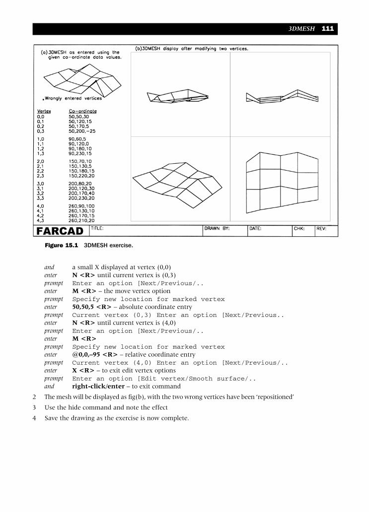
and a small X displayed at vertex (0,0)enter N <R> until current vertex is (0,3)prompt Enter an option [Next/Previous/..enter M <R> – the move vertex optionprompt Specify new location for marked vertexenter 50,50,5 <R> – absolute coordinate entryprompt Current vertex (0,3) Enter an option [Next/Previous..enter N <R> until current vertex is (4,0)prompt Enter an option [Next/Previous/..enter M <R>prompt Specify new location for marked vertexenter @0,0,–95 <R> – relative coordinate entryprompt Current vertex (4,0) Enter an option [Next/Previous/..enter X <R> – to exit edit vertex optionsprompt Enter an option [Edit vertex/Smooth surface/..and right-click/enter – to exit command
2 The mesh will be displayed as fig(b), with the two wrong vertices have been ‘repositioned’
3 Use the hide command and note the effect
4 Save the drawing as the exercise is now complete.
3DMESH 111
Figure 15.1 3DMESH exercise.
modelling with AutoCAD.qxd 17/06/2002 15:39 Page 111

Notes1 This example has been a brief introduction to the 3DMESH command
2 The command requires the user to enter all vertex values as coordinates and is thereforevery tedious to use. You can also reference existing objects if these are displayed
3 The Modify-Polyline command can be used with 3D meshes. This is the same as the 2Dmodify-polyline command
4 Selecting MESH from the 3D Objects dialogue box, will allow the user to create a 2Dmesh by:a) specifying the four corners of the meshb) entering the M and N sizes
5 The 3D MESH values M and N can be between 2 and 256
6 A 3D MESH is a single object
7 The command can be activated:a) by icon selection from the Surfaces toolbarb) from the menu bar with Draw-Surfacesc) by entering 3DMESH at the command line.
112 Modelling with AutoCAD 2002
modelling with AutoCAD.qxd 17/06/2002 15:39 Page 112

Ruled surfaceA ruled surface is a polygon mesh created between two defined boundaries selected bythe user. The objects which can be used to define the boundaries are lines, arcs, circles,points and 2D/3D polylines. The surface created is a ‘one-way’ mesh of straight linesdrawn between the two selected boundaries. The number of straight line meshes iscontrolled by the system variable SURFTAB1 which has an initial value of 6.
The ruled surface effect will be demonstrated by worked examples, the first being in 2Dto allow the user to become familiar with the basic terminology.
Example 11 Begin a new 2D drawing from scratch (metric) and create two layers, MOD (red) and
RULSUR (blue). Refer to Fig. 16.1
2 Display the Draw, Modify and Surfaces toolbars
Chapter 16
Figure 16.1 Ruled surface example 1 – usage and basic terminology.
modelling with AutoCAD.qxd 17/06/2002 15:39 Page 113

Pick points effect1 With layer MOD current, draw two lines and two three point arcs as fig(a) then make
layer RULSUR current
2 Select the RULED SURFACE icon from the Surfaces toolbar and:prompt Select first defining curverespond pick a point P1 on the first lineprompt Select second defining curverespond pick a point P2 on the first arcand a blue ruled surface is drawn between the two objects
3 Menu bar with Draw-Surfaces-Ruled Surface and:a) first defining curve prompt: pick point P3 on second lineb) second defining curve prompt: pick point P4 on second arcc) ruled surface drawn between the line and arc
4 The ruled surface drawn between selected objects is thus dependent on the pick pointpositions.
Effect of the SURFTAB1 system variable1 With layer MOD current draw a line and three point arc as fig(b)
2 Copy the line and arc to three other places on screen
3 Make layer RULSUR current
4 At the command line enter SURFTAB1 <R> and:prompt Enter new value for SURFTAB1<?>enter 6 <R>
5 At the command line enter RULESURF <R> and:prompt Select first defining curverespond pick a point on the first lineprompt Select second defining curverespond pick a point on the first arc
6 By entering SURFTAB1 at the command line, enter new values of 12, 24 and 36 and adda ruled surface between the other lines and arcs.
7 Notea) The system variable SURFTAB1 controls the display of the ruled surface effect, i.e.
the number of ‘strips’ added between the defining curves. b) The default value is 6. c) The value of SURFTAB1 to be used is dependent on the ‘size’ of the defining curves.
Open paths1 An open path is defined as a line, arc or open polyline
2 With layer MOD current draw some open paths as fig(c)
3 Using the ruled surface command and with SURTFAB1 set to your own value, add ruledsurfaces between the drawn open paths.
Closed paths1 A closed path is defined as a circle or closed polyline.
2 Draw some closed paths as fig(d) and add ruled surfaces between them.
114 Modelling with AutoCAD 2002
modelling with AutoCAD.qxd 17/06/2002 15:39 Page 114
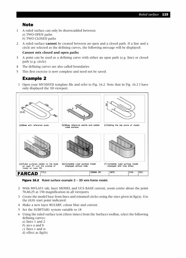
Note1 A ruled surface can only be drawn/added between:
a) TWO OPEN pathsb) TWO CLOSED paths
2 A ruled surface cannot be created between an open and a closed path. If a line and acircle are selected as the defining curves, the following message will be displayed:
Cannot mix closed and open paths
3 A point can be used as a defining curve with either an open path (e.g. line) or closedpath (e.g. circle)
4 The defining curves are also called boundaries
5 This first exercise is now complete and need not be saved.
Example 21 Open your MV3DSTD template file and refer to Fig. 16.2. Note that in Fig. 16.2 I have
only displayed the 3D viewport.
2 With MVLAY1 tab, layer MODEL and UCS BASE current, zoom centre about the point70,40,25 at 150 magnification in all viewports
3 Create the model base from lines and trimmed circles using the sizes given in fig(a). Usethe (0,0) start point indicated.
4 Make a new layer RULSRF, colour blue and current5 Set the SURFTAB1 system variable to 186 Using the ruled surface icon (three times) from the Surfaces toolbar, select the following
defining curves:a) lines 1 and 2b) arcs a and bc) lines v and wd) effect as fig(b)
Ruled surface 115
Figure 16.2 Ruled surface example 2 – 3D wire-frame model.
modelling with AutoCAD.qxd 17/06/2002 15:39 Page 115
7 Erase the ruled surface and create the top surface of the model by copying the baseobjects:a) from the point 0,0,0b) by @0,0,50 – fig(c)
8 With layer RULSRF still current, select the ruled surface icon and select the followingdefining curves as fig(c):a) lines 1 and 2 – ruled surface addedb) lines 3 and 1 – no ruled surface added and following message displayed:
Object not usable to define ruled surface – why?c) Explanation: when the second set of defined curves was being selected:
1. point 3 was picked satisfactorily2. point 1 could not be picked – you were picking the previous ruled surface added
between lines 1 and 2d) cancel the ruled surface command (ESC) and erase the added ruled surface
9 Make the following four new layers:R1 – red; R2 – blue; R3 – green; R4 – magenta
10 a) Make layer R1 currentb) Add a ruled surface to the base of the model (three needed)
11 a) Make layer R2 currentb) Freeze layer R1c) Add a ruled surface to the three ‘outside’ vertical planes of the model d) Thaw layer R1 – fig(d)
12 a) Make layer R3 currentb) Freeze layers R1 and R2c) Rule surface the top three defining curves of the model
13 a) Make layer R4 current and freeze layer R3b) Add a ruled surface to the three ‘inside’ vertical planes
14 a) Thaw layers R1, R2 and R3b) Model displayed a fig(e)
15 Menu bar with View-Hide to give fig(f)
16 Menu bar with View-Shade-Gouraud Shaded – impressive?
17 Return the model to wire-frame then save as MODR2002\RSRF1, it may be used in alater exercise
18 NoteWhen the ruled surface command is being used with adjacent surfaces, it isrecommended that:a) a layer be made for each ruled surface to be addedb) once a ruled surface has been added, that layer should be frozen before the next
surface is addedc) the new surface layers should be coloured for effect
19 Taska) Try the 3D orbit with the 3D viewport activeb) The two ‘ends’ of the model are ‘open’. A 3DFACE could be added to these ends?c) The original model was created from lines and circles/arcs. The base could have beencreated from a single polyline and then offset. Try this and add a ruled surface and notethat only one set of defining curves is required. What about SURFTAB1 with a polyline?
116 Modelling with AutoCAD 2002
modelling with AutoCAD.qxd 17/06/2002 15:39 Page 116

Example 3This example will investigate how a ruled surface can be added to a surface which hasa circular/slotted hole in it. The example will be in 2D, but the procedure is identical fora 3D model.
1 Begin a new 2D metric drawing from scratch and refer to Fig. 16.3
2 Make two new layers, MOD red (current) and RULSRF blue and set SURFTAB1 to 24
3 Using the LINE icon draw a square of side 60 with a 15 radius circle at the square ‘centre’– snap on helps
4 Using the Ruled Surface icon, pick any line of the square and the circle as the definingcurves. No ruled surface can be added because of the open/closed path effect – fig(a)
5 With the Polyline icon, draw a 60 sided square from 1–2–3–4–<R> as fig(b) and drawthe 15 radius circle. Add a ruled surface and the open/closed path message is displayedand no ruled surface is added.
6 Draw a closed polyline square using the points 1–2–3–4–close in the order given in fig(c).Draw the circle. With the ruled surface icon pick the defining curves indicated and a ruledsurface is added, but not as expected.
7 Draw a 60 sided square as a closed polyline and select the points 1–2–3–4–close in theorder given in fig(d). Draw the circle then add a ruled surface picking the defining curvesindicated. The added ruled surface is not quite ‘correct’ at the circle.
Ruled surface 117
Figure 16.3 Ruled surface example 3 – polylines and circles.
modelling with AutoCAD.qxd 17/06/2002 15:39 Page 117
8 Erase the ruled surface effect, set SURFTAB1 to 48 and repeat the ruled surface commandto give fig(e). Set SURFTAB1 back to 24.
9 Notea) When a ruled surface is added between two defined curves, the surface ‘begins at the
defined curve start points’. It is thus essential that the defined curves are:1 DRAWN IN THE SAME DIRECTION2 DRAWN FROM THE SAME ‘RELATIVE’ START POINT
b) Circular holes require to be drawn as two closed polyarcs
10 TaskUsing the information given in step 9, add ruled surfaces to the following modelsdisplayed in Fig. 16.3:a) fig(p): square drawn as a closed polyline and circle drawn as two closed polyarcs. Note
start pointsb) fig(q): square drawn as a closed polyline and circle drawn as two closed polyarcs. Note
that the start points differ from those in fig(p)c) fig(r): both the outer and inner perimeters are drawn as closed polylines/polyarcs. Note
the start pointsd) fig(s): the outer perimeter is drawn as four lines, and the inner as two arcs and two
lines.
11 When this task is complete, the exercise is finished. Save?
Example 4A ruled surface is one of the most effective surface modelling techniques, and I haveincluded another 3D model to demonstrate how it is used. The procedure when addinga ruled surface is basically the same with all models, this being:a) create the 3D wire-frame modelb) make new coloured layers for the surfaces to be addedc) use the ruled surface command with layers current as required.
1 Open your MV3DSTD template file and refer to Fig. 16.4
2 Make four new layers, R1 red, R2 blue, R3 green and R4 magenta
3 With MVLAY1 tab and layer MODEL current, restore UCS FRONT and make the lowerleft (3D) viewport active.
4 Select the POLYLINE icon and draw:Start point: 0,0Next point: @0,100Next point: Arc option, i.e. enter A <R>Arc endpt: @50,50 then right-click/enter
5 Centre each viewport about the point 50,75,0 at 175 mag
6 Offset the polyline by 20 ‘inwards’
7 Copy the two polylines from: 0,0, by: @0,0,–20
8 Change the viewpoint in the lower left viewport with the rotate option and angles:a) first prompt: 300b) second prompt: 30
9 Set SURFTAB1 to 18
10 Making each layer R1-R4 current, add a ruled surface to each ‘side’ of the model,remembering to freeze layers as in the second example.
118 Modelling with AutoCAD 2002
modelling with AutoCAD.qxd 17/06/2002 15:39 Page 118

11 Restore UCS BASE and polar array the complete model (crossing selection) using:a) Method: Total number of items & Angle to fillb) Centre point: X: 50 and Y: 10c) Total number of items: 4d) Angle to fill: 360e) Rotate items as copied: active
12 Hide, shade etc – impressive result?
13 Save the complete model as MODR2002\ARCHES for future recall
14 Note
The top ‘square’ of the arrayed arches – comments?
Summary1 A ruled surface can be added between lines, circles, arcs, points and polylines
2 The command can be activated in icon form, from the menu bar or by keyboard entry
3 The command can be used in 2D or 3D
4 A ruled surface CAN ONLY be added between:a) two open paths, e.g. lines, arcs, polylines (not closed)b) two closed paths, e.g. circles, closed polylines
5 Points can be used with open and closed paths
Ruled surface 119
Figure 16.4 Ruled surface example 4 – ARCHES.
modelling with AutoCAD.qxd 17/06/2002 15:39 Page 119

6 With closed paths, the correct effect can only be obtained if:a) the paths are drawn in the same directionb) the paths start at the ‘same relative point’
7 The system variable SURFTAB1 controls the number of ruled surface ‘strips’ addedbetween the two defining curves.
8 The default SURFTAB1 value is 6
AssignmentActivity 11: Ornamental flower bed of MACFARAMUS
MACFARAMUS designed some interesting artefacts for the famous lost city ofCADOPOLIS. One of his least known creations has the ‘hanging gardens’ for which hemade several unusual ornamental flower beds. It is one of these which you have to createas a 3D ruled surface model, the procedure being the same as in the examples:
1 Open your MV3DSTD template file, MVLAY1 tab, layer MODEL active
2 Create the wire-frame model from lines and trimmed circles using the sizes given withthe (0,0) start point. The vertical R50 arch requires the UCS RIGHT to be current andthe R30 side curve requires UCS FRONT. Use your discretion for any sizes omitted.
3 With UCS BASE, zoom centre about 90,50,50 at 200 mag.
4 Make four coloured layers
5 Add ruled surfaces to the ‘four sides’ of the model using the four new layers correctly.Use a SURFTAB1 value of 18 for most of the defining curves, but 6 for the ‘side’ line/arcselection.
6 Hide, shade, 3D orbit, save.
7 Notea) I suggest that you enter paper space and zoom-window the lower left viewport then
return to model space. This will make creating the wire-frame model and selectingthe defining curves easier
b) As an alternative to (a), create the model with the MODEL tab active
120 Modelling with AutoCAD 2002
modelling with AutoCAD.qxd 17/06/2002 15:39 Page 120
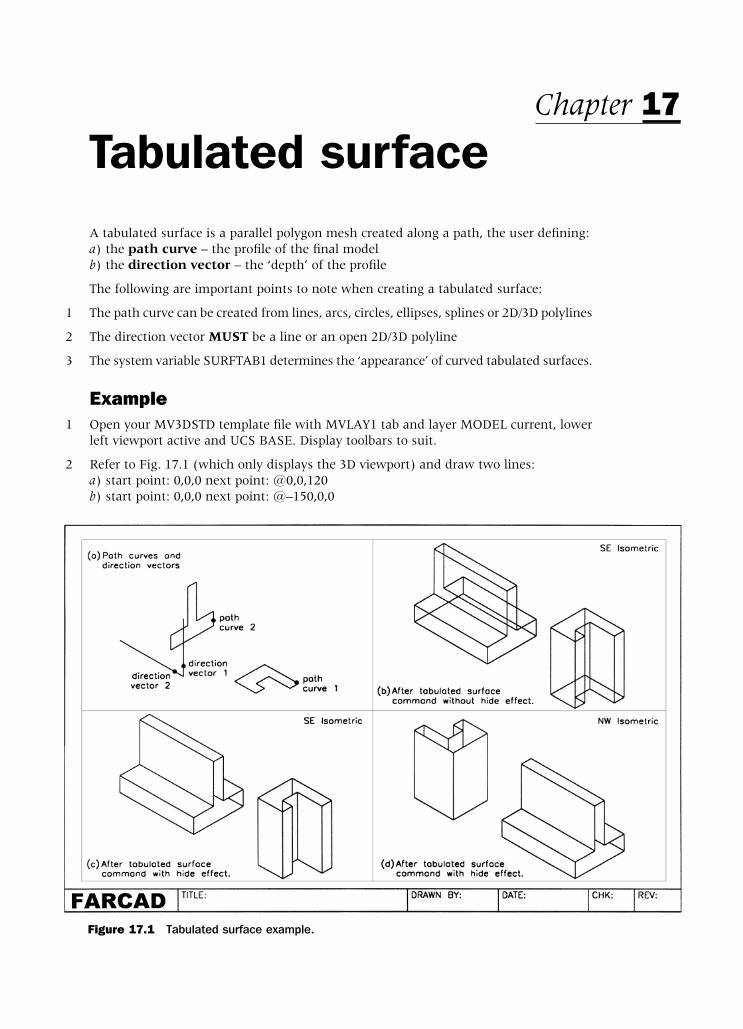
Tabulated surfaceA tabulated surface is a parallel polygon mesh created along a path, the user defining:a) the path curve – the profile of the final modelb) the direction vector – the ‘depth’ of the profile
The following are important points to note when creating a tabulated surface:
1 The path curve can be created from lines, arcs, circles, ellipses, splines or 2D/3D polylines
2 The direction vector MUST be a line or an open 2D/3D polyline
3 The system variable SURFTAB1 determines the ‘appearance’ of curved tabulated surfaces.
Example1 Open your MV3DSTD template file with MVLAY1 tab and layer MODEL current, lower
left viewport active and UCS BASE. Display toolbars to suit.
2 Refer to Fig. 17.1 (which only displays the 3D viewport) and draw two lines:a) start point: 0,0,0 next point: @0,0,120b) start point: 0,0,0 next point: @–150,0,0
Chapter 17
Figure 17.1 Tabulated surface example.
modelling with AutoCAD.qxd 17/06/2002 15:39 Page 121

3 Restore the appropriate UCS and draw two closed polylines with the following coordinatedata:UCS BASE UCS RIGHTStart: 70,50,0 Start: 20,20,–50Next: @50,0 Next: @100,0Next: @0,20 Next: @0,30Next: @–20,0 Next: @–40,0Next: @0,30 Next: @0,80Next: @50,0 Next: @–20,0Next: @0,20 Next: @0,–80Next: @–80,0 Next: @–40,0Next: close Next: close
4 Restore UCS BASE and zoom centre about –35,70,60 at 250 mag in all viewports
5 Select the TABULATED SURFACE icon from the Surfaces toolbar and:prompt Select object for path curverespond pick polyline 1 as fig(a)prompt Select object for direction vectorrespond pick line 1 at the end indicatedand a tabulated surface is added to the path curve
6 The added tabulated surface has a ‘depth’ equal to the length of the direction vector, i.e.120
7 Menu bar with Draw-Surfaces-Tabulated Surface and:prompt Select object for path curve respond pick polyline 2 as fig(a)prompt Select object for direction vector respond pick line 2 at the end indicated
8 Figure 17.1 displays (in 3D) the results of the tabulated surface operations:a) reference informationb) tabulated surfaces without hide at SE Isometric viewpointc) tabulated surfaces with hide at SE Isometric viewpointd) at a NW Isometric viewpoint with hide
9 Taska) Erase the tabulated surfaces to display the original path curvesb) Repeat the tabulated surface commands, but pick the direction vector lines at the
‘opposite ends’ from the exercise. The path curve will be ‘extruded’ in the oppositesense.
Summary1 A tabulated surface is a parallel polygon mesh
2 The command requires:a) a path curve – a single objectb) a direction vector – generally a line
3 The command can be used in 2D or 3D
4 The final surface orientation is dependent on the direction vector ‘pick point’
5 SURFTAB1 determines the surface appearance with curved objects
6 The command can be activated:a) in icon form from the Surfaces toolbarb) from the menu bar with Draw-Surfacesc) by entering TABSURF <R> at the command line.
122 Modelling with AutoCAD 2002
modelling with AutoCAD.qxd 17/06/2002 15:39 Page 122

Revolved surfaceA revolved surface is a polygon mesh generated by rotating a path curve (profile) aboutan axis, the user selecting:a) the path curve – a single object, e.g. a line, arc, circle or 2D/3D polylineb) the axis of revolution – generally a line, but can be an open or closed polyline.
The generated mesh is controlled by two system variables:a) SURFTAB1: controls the mesh in the direction of the revolutionb) SURFTAB2: defines any curved elements in the profilec) the default value for both variables is 6
Example 11 Open the MV3DSTD template file, MVLAY1 tab and layer MODEL current, UCS BASE
and refer to Fig. 18.1
2 Make the lower right viewport active and display toolbars
3 Draw two lines:a) start point: 0,0 next point: @100,0b) start point: 0,0 next point: @0,100
4 Set SURFTAB1 to 16 and SURFTAB2 to 6 – command line entry
Chapter 18
Figure 18.1 Revolved surface example 1.
modelling with AutoCAD.qxd 17/06/2002 15:39 Page 123

5 Using the polyline icon from the Draw toolbar, create a CLOSED polyline shape usingthe reference sizes given in Fig. 18.1. The start point is to be 50,50
Note The actual polyline shape is not that important. Use your discretion/own design, but tryand keep to the overall reference sizes given.
6 Select the REVOLVED SURFACE icon from the Surfaces toolbar and:prompt Select object to revolverespond pick any point on the polylineprompt Select object that defines the axis of revolutionrespond pick the Y axis lineprompt Specify start angle<0> and enter: 0 <R>prompt Specify included angle (+ = ccw, – = cw)<360>enter 360 <R>
7 A revolved surface model will be displayed in each viewport
8 In all viewport, zoom centre about 0,120,0 at 350 magnification
9 Hide each viewport – fig(a)
10 Erase the revolved surface (regen needed?) to display the original polyline shape andfrom the menu bar select Draw-Surfaces-Revolved Surface and:a) object to revolve: pick the polyline shapeb) object to define axis of revolution: pick the X axis linec) start angle: 0d) included angle: 360
11 Zoom centre about 100,0,0 at 400 magnification
12 Hide the viewports – fig(b)
13 Save if required, as this first exercise is complete.
Example 21 Open the MV3DSTD template file, MVLAY1 tab, layer MODEL, UCS BASE with the lower
right viewport active
2 Refer to Fig. 18.2
3 Draw a line from 0,0 to @0,250
4 With the polyline icon, draw an OPEN polyline shape using the sizes in fig(a) as areference. The start point is to be (0,50) but the final polyline shape is at your discretionas it is your wine glass design.
5 Set SURFTAB1 to 18 and SURFTAB2 to 6
6 At the command line enter REVSURF <R> and:a) object to revolve: pick the polyline shapeb) object to define axis of revolution: pick the linec) start angle: enter 0d) included angle: enter 270
7 Set the following 3D viewpoints in the named viewports:Top left: NE Isometric Top right: NW IsometricLower left: SE Isometric Lower right: SW Isometric
8 Zoom centre about 0,120,0 at 200 magnification
9 Hide the viewports – fig(b)
10 Save if required
124 Modelling with AutoCAD 2002
modelling with AutoCAD.qxd 17/06/2002 15:39 Page 124

Summary1 The revolved surface command can be used to produce very complex surface models from
relatively simple profiles
2 The resultant polygon mesh is controlled by the two system variables, SURFTAB1 andSURFTAB2:a) SURFTAB1: controls the mesh in the direction of rotationb) SURFTAB2: controls the display of curved elements in the profile
3 The start angle can vary between 0 and 360. A start angle of 0 means that that the surfaceis to begin on the current drawing plane. This is generally what is required.
4 The included angle allows the user to define the angle the path curve is to be revolvedthrough. The 360 default value gives a complete revolution, but ‘cut-away’ models canbe obtained with angles less than 360
5 The direction of the revolved surface is controlled by the sign of the included angle and:a) +ve for anti-clockwise revolved surfacesb) –ve for a clockwise revolution
6 The command can be activated by icon, from the menu bar or by command line entry.
Revolved surface 125
Figure 18.2 Revolved surface example 2.
modelling with AutoCAD.qxd 17/06/2002 15:39 Page 125

AssignmentMACFARAMUS designed a garden furniture arrangement for the gardens inCADOPOLIS. This garden furniture set complemented the ornamental flower bed createdas a ruled surface. You need to create two profiles and revolve them about two differentaxes. Adding colour to the revolved surfaces greatly enhances the model appearance withshading and rendering.
Activity 12: Garden furniture set of MACFARAMUS.
1 Use your MV3DSTD template file – MVLAY1 tab
2 Make the top right viewport active and restore UCS FRONT
3 Draw two polyline profiles using the reference data given. Use your discretion for sizesnot given, or design your own table and chair. Also draw two vertical lines for the axesof revolution.
4 Set SURFTAB1 to 18 and SURFTAB2 to 6
5 Revolve the profiles about vertical lines
6 Change the colour of the revolved chair to green and the table to blue
7 Restore UCS BASE and make the lower left viewport active
8 Polar array the chair for five items about the point (0,0) with rotation
9 Hide the viewports, then REGENALL and save as MODR2002\GARDEN
10 Try the following with the Model tab active:a) Gouraud shadeb) Use the 3D orbit command
11 Make sure this model has been saved.
126 Modelling with AutoCAD 2002
modelling with AutoCAD.qxd 17/06/2002 15:39 Page 126

Edge surfaceAn edge surface is a 3D polygon mesh stretched between four touching edges. The edgescan be combinations of lines, arcs, polylines or splines but must form a closed loop.
The edge surface mesh is controlled by the system variables:a) SURFTAB1: the M facets in the direction of the first edge selectedb) SURFTAB2: the N facets in the direction of the edges adjacent to the first selected edge
Three examples will be used to demonstrate the command, the first being in 2D, thesecond to allow us to use the editing features of a polygon mesh, and the third will usesplines as the four touching edges.
Example 1 (2D edge surfaces)1 Open any 2D drawing and make two layers, EDGE colour red and MESH colour blue
2 Refer to Fig. 19.1 and display toolbars as required. Erase all objects
Chapter 19
Figure 19.1 Edge surface example 1 – 2D application.
modelling with AutoCAD.qxd 17/06/2002 15:39 Page 127

3 With layer EDGE current, create the following touching edges similar in layout to fig(a):a) four linesb) four three point arcsc) four single 90deg polyline arcs (use CE option)
4 Set SURFTAB1 to 10 and SURFTAB2 to 7
5 Select the EDGE SURFACE icon from the Surfaces toolbar and: prompt Select object 1 for surface edgerespond pick a point on any lineprompt Select object 2 for surface edgerespond pick a point on another lineprompt Select object 3 for surface edgerespond pick a point on a third lineprompt Select object 4 for surface edgerespond pick a point on the fourth line
6 A 10x7 surface mesh is stretched between the four touching lines as fig(a1)
7 a) Erase the added edge surfaceb) Set SURFTAB1 and SURFTAB2 to 18c) Menu bar with Draw-Surfaces-Edge Surface and pick the four touching lines in
any orderd) The edge surface mesh is displayed as fig(a2)
8 At the command line enter EDGESURF <R> and pick the four arcs to display the edgesurface mesh as fig(b)
9 Set both SURFTAB1 and SURFTAB2 to 10 and add an edge surface mesh between tofour touching polyarcs – fig(c). The result of this mesh is quite interesting?
This completes the first exercise and it need not be saved.
Example 2 (a 3D edge surface mesh)1 Open your MV3DSTD template file (MVLAY1 tab)
2 Refer to Fig. 19.2
3 With layer MODEL, UCS BASE and the lower left viewport active, use the LINE icon todraw the four touching lines:Start point: 0,0,0Next point: 150,0,–20 Next point: 180,200,30Next point: 40,120,50 Next point: close
4 The four lines will be displayed as fig(a)
5 Centre each viewport about the point 90,100,25 at 250 mag.
6 Make a new layer, MESH colour blue and current
7 Set both SURFTAB1 and SURFTAB2 to 10
8 Using the edge surface icon, pick the four lines in the order indicated 1–2–3–4 as fig(a)
9 An edge surface mesh will be stretched between the four lines as fig(b)
10 In paper space, zoom the 3D viewport and return to model space
128 Modelling with AutoCAD 2002
modelling with AutoCAD.qxd 17/06/2002 15:39 Page 128

11 Menu bar with Modify-Object-Polyline and:prompt Select polylinerespond pick any point on meshprompt Enter an option [Edit vertex/Smooth surface/..enter E <R> – the edit vertex optionprompt Current vertex (0,0) then Enter an option [Next/Previous/..and an X is displayed at the 0,0 vertex – leftmost?enter U <R> until X is at vertex (10,0) and:prompt Current vertex (10,0)then Enter an option [Next/Previous/..enter M <R> – the move optionprompt Specify new location for marked vertexenter @0,0,60 <R>and DO NOT EXIT COMMAND
12 We now want to alter other vertices of the mesh to create a raised effect. This will beachieved by:a) moving the X to the required vertices b) using the M optionc) entering the required relative vertex coordinates
Edge surface 129
Figure 19.2 Edge surface example 2 – 3D with edit vertices.
modelling with AutoCAD.qxd 17/06/2002 15:39 Page 129

13 Use the N/D/L/R/U options and enter the following new locations for the named vertices:relative movement vertices@0,0,50 9,0 10,1@0,0,40 8,0 9,1 10,2@0,0,30 7,0 8,1 9,2 10,3@0,0,20 6,0 7,1 8,2 9,3 10,4@0,0,10 5,0 6,1 7,2 8,3 9,4 10,5
14 When all the new vertex locations have been entered:a) enter X <R> to exit the edit vertex optionb) then enter X <R> to end the command
15 The mesh will be displayed with a ‘raised corner’ as fig(c)
16 At the command line enter PEDIT <R> then:a) pick any point on the meshb) enter E <R> for the edit vertex optionc) use the N/U/R/L/D entries to move the X to the following named vertices and with
the M (move option), enter the following new locations:relative movement vertices@0,0,–80 4,10@0,0,–50 3,10 4,9 5,10@0,0,–30 2,10 3,9 4,8 5,9 6,10@0,0,–10 1,10 2,9 3,8 4,7 5,8 6,9 7,10
d) exit the vertex option with X <R>e) exit the polyline edit command with X <R>
17 These vertex modifications have produced a v-type notch in the mesh as fig(d)
18 Paper space and zoom-previous then model space. Freeze the MODEL layer
19 The complete four viewport configuration of the edge surface mesh is displayed in fig(e)
20 The exercise is now complete – save if required.
21 Now investigate the effect of the smooth surface option (S) on the mesh
Example 3 (an edge surface mesh created from splines)This example will demonstrate how an edge surface can be stretched between four splinecurves to simulate a car body panel.
1 Open your MV3DSTD template file as usual, i.e. MVLAY1 tab, layer MODEL and UCS BASE
2 Zoom centre about the point (–100,50,50) at 225 magnification in the 3D viewport and200 in the other three
3 With the lower left viewport active, refer to Fig. 19.3 and by selecting the SPLINE iconfrom the Draw toolbar, draw four spline curves using the following coordinateinformation. Use the start and end coordinates as the start and end tangents, indicatedby (S) and (E) in the following data table:spline 1 spline 2 spline 3 spline 40,0,0 (S) –200,0,0 (S) –200,80,105 (S) 0,0,0 (S)–200,0,0 (E) –200,0,100 0,100,105 (E) 0,0,110<RETURN> –200,80,105 (E) <RETURN> 0,100,105 (E)
<RETURN> <RETURN>
4 The four spline curves will be displayed as fig(a)
5 Make a new layer, MESH colour blue and current
130 Modelling with AutoCAD 2002
modelling with AutoCAD.qxd 17/06/2002 15:39 Page 130
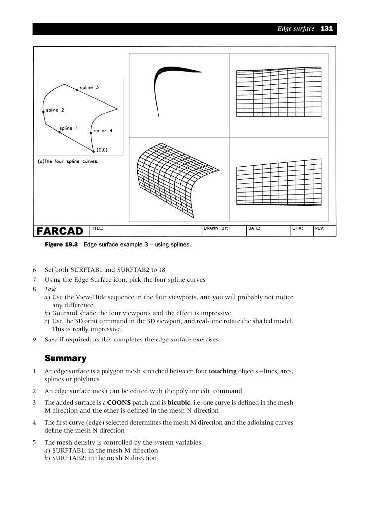
6 Set both SURFTAB1 and SURFTAB2 to 18
7 Using the Edge Surface icon, pick the four spline curves
8 Taska) Use the View-Hide sequence in the four viewports, and you will probably not notice
any differenceb) Gouraud shade the four viewports and the effect is impressivec) Use the 3D orbit command in the 3D viewport, and real-time rotate the shaded model.
This is really impressive.
9 Save if required, as this completes the edge surface exercises.
Summary1 An edge surface is a polygon mesh stretched between four touching objects – lines, arcs,
splines or polylines
2 An edge surface mesh can be edited with the polyline edit command
3 The added surface is a COONS patch and is bicubic, i.e. one curve is defined in the meshM direction and the other is defined in the mesh N direction
4 The first curve (edge) selected determines the mesh M direction and the adjoining curvesdefine the mesh N direction
5 The mesh density is controlled by the system variables:a) SURFTAB1: in the mesh M directionb) SURFTAB2: in the mesh N direction
Edge surface 131
Figure 19.3 Edge surface example 3 – using splines.
modelling with AutoCAD.qxd 17/06/2002 15:39 Page 131

6 The default value for SURFTAB1 and SURFTAB2 is 6
7 The type of mesh stretched between the four curves is controlled by the SURFTYPEsystem variable and:a) SURFTYPE 5 – Quadratic B-splineb) SURFTYPE 6 – Cubic B-spline (default)c) SURFTYPE 8 – Bezier curve
8 The SURFTYPE variable controls the appearance of all mesh curves.
AssignmentMACFARAMUS was contracted by the emperor TOOTENCADUM to create a flat toppedhill for a future project.
The activity is very similar to the second example, i.e. an edge surface has to have severalof its vertices modified to give a ‘flat-top hill’ effect. The process is quite tedious, butpersevere with it as it is needed for another activity in a later chapter.
Activity 13: The flat topped hill made by MACFARAMUS.
1 Use your MV3DSTD template file with UCS BASE as usual
2 Zoom centre about 0,0,50 at 400 magnification originally
3 With layer MODEL, create four touching polyline arcs of radius 200 with 0,0 as the arccentre point. If you are unsure of this, use the Centre, Start, End ARC option.
4 Make a new layer called HILL, colour green and current
5 Set SURFTAB1 and SURFTAB2 to 20
6 Add an edge surface to the four touching arcs
7 In paper space, zoom the 3D viewport then return to model space
8 Use the Modify-Object-Polyline (PEDIT) command with the Edit Vertex option to movethe following vertices by @0,0,100:a) 6,9 6,10 6,11b) 7,7 7,8 7,9 7,10 7,11 7,12 7,13c) 8,7 8,8 8,9 8,10 8,11 8,12 8,13d) 9,6 9,7 9,8 9,9 9,10 9,11 9,12 9,13 9,14e) 10,6 10,7 10,8 10,9 10,10 10,11 10,12 10,13 10,14f) 11,6 11,7 11,8 11,9 11,10 11,11 11,12 11,13 11,14g) 12,7 12,8 12,9 12,10 12,11 12,12 12,13h) 13,7 13,8 13,9 13,10 13,11 13,12 13,13i) 14,9 14,10 14,11
9 Notea) The named vertices all lie within a circle of radius 100b) Use the N/U/D/L/R entries of the edit vertex option until the named vertex is displayedthen use the M option with an entry of @0,0,100
10 When all the vertices have been modified, optimise your viewpoints. I used four differentVPOINT-ROTATE values and the effect with hide was quite ‘pleasing’
11 Save this drawing as MODR2002\HILL as it will be used with a later activity.
12 The View-Shade-Gouraud Shaded effect in any 3D viewport with the 3D orbit commandis very interesting. You can rotate the model to ‘see inside’ the raised part of the edgesurface.
132 Modelling with AutoCAD 2002
modelling with AutoCAD.qxd 17/06/2002 15:39 Page 132
3D polylineA 3D polyline is a continuous object created in 3D space. It is similar to a 2D polyline,but does not possess the 2D versatility, i.e. there are no variable width or arc optionsavailable with a 3D polyline. The benefit of a 3D polyline is that it allows x,y,z coordinatesto be used. A 2D polyline can only be created in the plane of the current UCS.
ExampleThis exercise will create a series of hill contours from splined 3D polylines, so:
1 Open your MV3DSTD template file, MVLAY1 tab with the lower left viewport active andUCS BASE.
2 Refer to Fig. 20.1 and make the following new layers:LEVEL1, LEVEL2, LEVEL3, LEVEL4 – all colour greenPATH1: red; PATH2: blue; PATH3: magenta
3 With layer LEVEL1 current, menu bar with Draw-3Dpolyline and:prompt Specify start point of polyline and enter: 0,50,0 <R>prompt Specify endpoint of line and enter: 50,0,0 <R>prompt Specify endpoint of line and enter: 150,0,0 <R>prompt Specify endpoint of line and enter: 220,60,0 <R>prompt Specify endpoint of line and enter: 260,140,0 <R>prompt Specify endpoint of line and enter: 170,180,0 <R>prompt Specify endpoint of line and enter: 20,160,0 <R>prompt Specify endpoint of line and enter: c <R>
4 Make layer LEVEL2 current and at the command line enter 3DPOLY <R> and:prompt Specify start point of polyline and enter: 40,60,50 <R>prompt Specify endpoint of line and enter: 80,20,50 <R>prompt Specify endpoint of line and enter: 140,35,50 <R>prompt Specify endpoint of line and enter: 200,100,50 <R>prompt Specify endpoint of line and enter: 130,140,50 <R>prompt Specify endpoint of line and enter: 60,130,50 <R>prompt Specify endpoint of line and enter: c <R>
5 With layers LEVEL3 and LEVEL4 current, use the 3D polyline command with thefollowing coordinate values:
Level3 Level4Start point 70,70,100 85,70,125Endpoint 80,35,100 90,50,125Endpoint 130,45,100 130,60,125Endpoint 170,90,100 130,80,125Endpoint 100,120,100 closeEndpoint close
Chapter 20
modelling with AutoCAD.qxd 17/06/2002 15:39 Page 133

6 Menu bar with Modify-Object-Polyline and:prompt Select polylinerespond pick the 3D polyline created at level 1prompt Enter an optionenter S <R> – the spline optionprompt Enter an optionenter X <R> – the exit command option
7 The selected polyline will be displayed as a splined curve
8 Use the S option of the Edit Polyline command to spline the other three 3D polylines
9 Zoom centre about 120,90,60 at 200 magnification in all viewports
10 With layer PATH1 current, use the 3D polyline command with the following entries:Start: 0,50,0 – level 1 pointEndpoint: 60,130,50 – level 2 pointEndpoint: 100,120,100 – level 3 pointEndpoint: 130,60,125 – level 4 pointEndpoint: <R>
11 This 3D polyline is a path ‘up the hill’ and each entered coordinate value is a point onthe level 1,2,3,4 contours
12 Spline this polyline, and it does not pass through the entered coordinates
134 Modelling with AutoCAD 2002
Figure 20.1 3D polyline example.
modelling with AutoCAD.qxd 17/06/2002 15:39 Page 134

13 Taska) Using the ID command, identify the coordinates of the points A, B and C where PATH1
‘crosses’ the level 2, 3 and 4 contours. My values were:ptA: 55.06, 101.57, 50ptB: 95.42, 101.91, 100ptC: 127.07, 65.65, 125
b) With layer PATH2 current, create a 3D polyline as a ‘path down the hill’, this path tobe drawn as a vertical line in the top (lower right) viewport. It has to ‘touch’ eachcontour, and if possible, be the shortest distance (ortho on helps, as does OSNAPnearest). Do not spline this path. Find the distance from top to bottom for this path.My value was 135.51.
c) With layer PATH3 current, create another un-splined 3D polyline which is to ‘join thefour level right-ends’ in the top right viewport. Find the distance between each levelfor this path.My three values were:1–2: 82.812–3: 57.693–4: 38.26
14 The exercise is now complete. Save if required.
Summary1 A 3D polyline is a single object and can be used with x,y,z coordinate entry
2 A 3D polyline can be edited with options of Edit vertex, Spline and decurve
3 3D polylines cannot be displayed with varying width or with arc segments.
4 The command is activated from the menu bar or by command line entry.
3D polyline 135
modelling with AutoCAD.qxd 17/06/2002 15:39 Page 135
3D objectsAutoCAD has nine pre-defined 3D objects, these being box, pyramid, wedge, dome,sphere, cone (and cylinder), torus, dish and mesh. They are considered as ‘meshes’ andcan be displayed with hide, shade and render.
To demonstrate some of these objects:
1 Open your MV3DSTD template file, with MVLAY1 tab, layer MODEL, UCS BASE andthe lower left viewport active.
2 Refer to Fig. 21.1 and display the Surfaces toolbar
3 In the steps which follow, reason out the coordinate entry values
4 Select the BOX icon from the Surfaces toolbar and:prompt Specify corner point of box and enter: 0,0,0 <R>prompt Specify length of box and enter: 150 <R>prompt Specify width of box and enter: 120 <R>prompt Specify height of box and enter: 100 <R>prompt Specify rotation angle of box about Z axis and enter: 0 <R>
5 A red box will be displayed at the 0,0,0 origin point
6 Menu bar with Draw-Surfaces-3D Surfaces and:prompt 3D Objects dialogue boxrespond pick Wedge then OKprompt Specify corner point of wedge and enter: 150,0,0 <R>prompt Specify length of wedge and enter: 80 <R>prompt Specify width of wedge and enter: 70 <R>prompt Specify height of wedge and enter: 150 <R>prompt Specify rotation angle of wedge about Z axis and enter: –10 <R>
7 At the command line enter CHANGE <R> and:prompt Select objects and pick the wedge then right-clickprompt Specify change point or [Properties] and enter: P <R>prompt Enter property to change and enter: C <R> – colour optionprompt Enter new colour and enter: 14 <R>prompt Enter property to change and <RETURN>
8 Using the icons from the Surfaces toolbar, or the 3D Objects dialogue box, create thefollowing two 3D objects:Cone Cylinder (using cone object)Base centre: 50,70,100 Base centre: 75,0,50Radius for base: 50 Radius for base: 50Radius for top: 0 Radius for top: 50Height: 85 Height: 90Number of segments: 16 Number of segments: 16Colour: green Colour: blue
9 Restore UCS RIGHT and with the ROTATE icon from the Modify toolbar:a) pick the blue cylinder then right-clickb) base point: 0,50c) rotation angle: 90
Chapter 21
modelling with AutoCAD.qxd 17/06/2002 15:39 Page 136
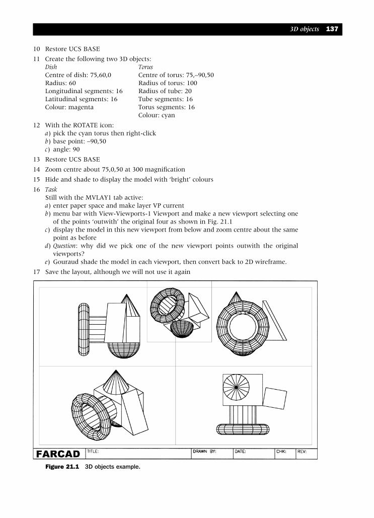
10 Restore UCS BASE
11 Create the following two 3D objects:Dish TorusCentre of dish: 75,60,0 Centre of torus: 75,–90,50Radius: 60 Radius of torus: 100Longitudinal segments: 16 Radius of tube: 20Latitudinal segments: 16 Tube segments: 16Colour: magenta Torus segments: 16
Colour: cyan
12 With the ROTATE icon:a) pick the cyan torus then right-clickb) base point: –90,50c) angle: 90
13 Restore UCS BASE
14 Zoom centre about 75,0,50 at 300 magnification
15 Hide and shade to display the model with ‘bright’ colours
16 TaskStill with the MVLAY1 tab active:a) enter paper space and make layer VP currentb) menu bar with View-Viewports-1 Viewport and make a new viewport selecting one
of the points ‘outwith’ the original four as shown in Fig. 21.1c) display the model in this new viewport from below and zoom centre about the same
point as befored) Question: why did we pick one of the new viewport points outwith the original
viewports?e) Gouraud shade the model in each viewport, then convert back to 2D wireframe.
17 Save the layout, although we will not use it again
3D objects 137
Figure 21.1 3D objects example.
modelling with AutoCAD.qxd 17/06/2002 15:39 Page 137
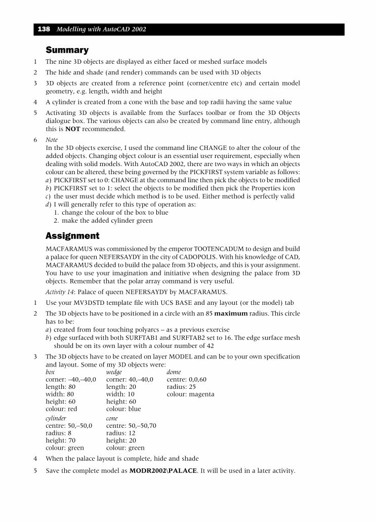
Summary1 The nine 3D objects are displayed as either faced or meshed surface models
2 The hide and shade (and render) commands can be used with 3D objects
3 3D objects are created from a reference point (corner/centre etc) and certain modelgeometry, e.g. length, width and height
4 A cylinder is created from a cone with the base and top radii having the same value
5 Activating 3D objects is available from the Surfaces toolbar or from the 3D Objectsdialogue box. The various objects can also be created by command line entry, althoughthis is NOT recommended.
6 NoteIn the 3D objects exercise, I used the command line CHANGE to alter the colour of theadded objects. Changing object colour is an essential user requirement, especially whendealing with solid models. With AutoCAD 2002, there are two ways in which an objectscolour can be altered, these being governed by the PICKFIRST system variable as follows:a) PICKFIRST set to 0: CHANGE at the command line then pick the objects to be modifiedb) PICKFIRST set to 1: select the objects to be modified then pick the Properties iconc) the user must decide which method is to be used. Either method is perfectly validd) I will generally refer to this type of operation as:
1. change the colour of the box to blue2. make the added cylinder green
AssignmentMACFARAMUS was commissioned by the emperor TOOTENCADUM to design and builda palace for queen NEFERSAYDY in the city of CADOPOLIS. With his knowledge of CAD,MACFARAMUS decided to build the palace from 3D objects, and this is your assignment.You have to use your imagination and initiative when designing the palace from 3Dobjects. Remember that the polar array command is very useful.
Activity 14: Palace of queen NEFERSAYDY by MACFARAMUS.
1 Use your MV3DSTD template file with UCS BASE and any layout (or the model) tab
2 The 3D objects have to be positioned in a circle with an 85 maximum radius. This circlehas to be:a) created from four touching polyarcs – as a previous exerciseb) edge surfaced with both SURFTAB1 and SURFTAB2 set to 16. The edge surface mesh
should be on its own layer with a colour number of 42
3 The 3D objects have to be created on layer MODEL and can be to your own specificationand layout. Some of my 3D objects were:box wedge domecorner: –40,–40,0 corner: 40,–40,0 centre: 0,0,60length: 80 length: 20 radius: 25width: 80 width: 10 colour: magentaheight: 60 height: 60colour: red colour: bluecylinder conecentre: 50,–50,0 centre: 50,–50,70radius: 8 radius: 12height: 70 height: 20colour: green colour: green
4 When the palace layout is complete, hide and shade
5 Save the complete model as MODR2002\PALACE. It will be used in a later activity.
138 Modelling with AutoCAD 2002
modelling with AutoCAD.qxd 17/06/2002 15:39 Page 138

3D geometrycommandsAll AutoCAD commands can be used in 3D but there are three commands which arespecific to 3D models, these being 3D Array, Mirror 3D and Rotate 3D. In this chapterwe will investigate these three commands and how to use the Align, Extend and Trimcommands with 3D models.
Getting startedTo investigate the 3D commands, we will create a new model from 3D Objects, so:
1 Begin a new drawing with your MV3DSTD template file
2 For this exercise it is recommended that the user works with the Model tab active so:a) select the Model tabb) layer MODEL and UCS BASE currentc) pan so that the UCS BASE icon is at the lower centre of the screen and alter the
viewpoint with the command line entry VPOINT <R> then R <R> (rotate option)and enter angles of 300 and 30
d) refer to Fig. 22.1 which displays the 3D viewport only
3 Select the BOX icon from the Surfaces toolbar and:a) corner: 0,0,0b) length: 100; width: 100; height: 40; Z rotation: 0c) colour: red
4 Select the WEDGE icon from the Surfaces toolbar and:a) corner: 0,0,40 b) length: 30; width: 30; height: 30; Z rotation: 0c) colour: blue
5 Zoom to a scale factor of 1
6 The two 3D objects will be displayed as fig(a)
Chapter 22
modelling with AutoCAD.qxd 17/06/2002 15:39 Page 139

Rotate 3DUsing the menu bar sequence Modify-Rotate or selecting the ROTATE icon from theModify toolbar results in a 2D command, i.e. the selected objects are rotated in thecurrent XY plane. Objects can be rotated in 3D relative to the X, Y and Z axes with theRotate 3D command. The command will be demonstrated by rotating the blue wedgeand then the complete model.
Rotating the wedge1 From the menu bar select Modify-3D Operation-Rotate 3D and:
prompt Select objectsrespond pick the blue wedge then right-clickprompt Specify first point on axis or define axis by [Object/
Last/..enter X <R> – the X axis optionprompt Specify a point on the X axis<0,0,0>enter 0,0,40 <R> – why these coordinates?prompt Specify rotation angleenter 90 <R>
2 The blue wedge is rotated about the x-axis as Fig. 22.1(b)
140 Modelling with AutoCAD 2002
Figure 22.1 The 3DGEOM model for the 3D commands.
modelling with AutoCAD.qxd 17/06/2002 15:39 Page 140

3 Activate the Rotate 3D command and:prompt Select objectsenter pick the blue wedge the right-clickprompt Rotate 3D options enter Z <R> – the Z axis optionprompt Specify a point on Z axis<0,0,0>enter 0,0,0 <R>prompt Specify rotation angleenter 90 <R>
4 The blue wedge is now aligned as required – fig(c)
5 Select the ARRAY icon from the Modify toolbar and with the Array dialogue box select:a) Type: Polar Arrayb) Objects: the blue wedgec) Center point: X: 50 and Y: 50d) Method: Total number of items & Angle to fille) Total items: 4f) Angle to fill: 360g) Rotate items as copied: active
6 The blue wedge is arrayed to the four corners of the box as fig(d)
7 With the Rotate 3D command:a) pick wedges 1 and 2 then right-click b) enter Y <R> as the defined axisc) enter 100,0,40 <R> as a point on axis – why this entry?d) enter 90 <R> as the rotation angle
8 Now move these two rotated wedges from 0,0 by @–30,0
9 The final result is fig(e) and can be saved as MODR2002\3DGEOM for future recall.
Rotating the model1 Model 3DGEOM on the screen in model tab with UCS BASE and layer MODEL current.
Refer to Fig. 22.2 (3D only)
2 Menu bar with Modify-3D Operation-Rotate 3D and:prompt Select objectsrespond window the complete model then right-clickprompt Specify first point on axis or define axisenter X <R> – the X axis optionprompt Specify a point on the X axis respond right-click, i.e. accept the 0,0,0 default pointprompt Specify rotation angle and enter: 45 <R>then PAN if required then HIDE – fig(b)
3 At the command line enter ROTATE3D <R> and:prompt Select objectsrespond window the model then right-clickprompt Specify first point on axis or define axisenter Z <R> – the Z axis optionprompt Specify a point on Z axis<0,0,0> and: right-clickprompt Specify rotation angle and enter: 60 <R>then PAN to suit and HIDE – fig(c)
3D geometry commands 141
modelling with AutoCAD.qxd 17/06/2002 15:39 Page 141
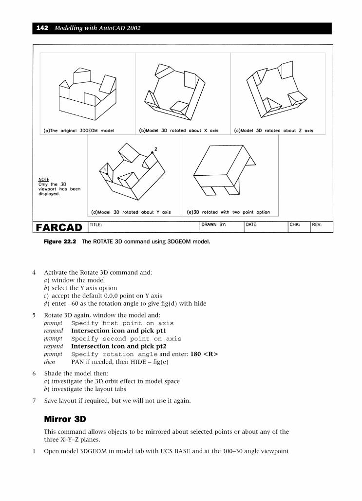
4 Activate the Rotate 3D command and:a) window the modelb) select the Y axis optionc) accept the default 0,0,0 point on Y axisd) enter –60 as the rotation angle to give fig(d) with hide
5 Rotate 3D again, window the model and:prompt Specify first point on axisrespond Intersection icon and pick pt1prompt Specify second point on axisrespond Intersection icon and pick pt2prompt Specify rotation angle and enter: 180 <R>then PAN if needed, then HIDE – fig(e)
6 Shade the model then:a) investigate the 3D orbit effect in model spaceb) investigate the layout tabs
7 Save layout if required, but we will not use it again.
Mirror 3DThis command allows objects to be mirrored about selected points or about any of thethree X–Y–Z planes.
1 Open model 3DGEOM in model tab with UCS BASE and at the 300–30 angle viewpoint
142 Modelling with AutoCAD 2002
Figure 22.2 The ROTATE 3D command using 3DGEOM model.
modelling with AutoCAD.qxd 17/06/2002 15:39 Page 142

2 Refer to Fig. 22.3 which again only displays the 3D viewport
3 Menu bar with Modify-3D Operation-Mirror 3D and:prompt Select objectsrespond window the model then right-clickprompt Specify first point on mirror plane (3 points) or [Object/
Last/..enter XY <R> – the XY plane optionprompt Specify point on XY plane<0,0,0> and: right clickprompt Delete source objects<Yes/No> and enter: Y <R>then PAN to suit – fig(b)
4 The model at this stage has the AMBIGUITY effect of all 3D models, i.e. are you lookingdown or looking up? Hence HIDE!
5 At the command line enter MIRROR3D <R> and:prompt Select objectsrespond window the model then right-clickprompt Specify first point on mirror planerespond Intersection icon and pick pt1prompt Specify second point on mirror planerespond Intersection icon and pick pt2prompt Specify third point on mirror planerespond Intersection icon and pick pt3prompt Delete source object<Yes/No> and enter: Y <R>then PAN to suit, then HIDE – fig(c)
3D geometry commands 143
Figure 22.3 The MIRROR 3D command using 3DGEOM model.
modelling with AutoCAD.qxd 17/06/2002 15:39 Page 143

6 Activate the Mirror 3D command and:a) window the model the right-clickb) select the YZ plane optionc) pick intersection of point A as a point on the planed) enter Y to delete source objects prompte) pan and hide – fig(d)
7 Using the Mirror 3D command:a) window the model the right-clickb) select the ZX optionc) enter –50,–50 as a point on the ZX planed) accept the N default delete source objects optione) pan and hide – fig(e)
8 Shade and 3D orbit, then investigate the layout tabs
9 Save if required. We will not refer to this drawing again.
3D ArrayThe 3D array command is similar in operation to the 2D array. Both rectangular and polararrays are possible, the rectangular array having rows and columns as well as levels inthe Z direction. The result of a 3D polar array requires some thought!
Rectangular1 Open the 3DGEOM drawing, UCS BASE, Model tab active and refer to Fig. 22.4 which
displays the MVLAY1 tab
2 At the command line enter 3DARRAY <R> and:prompt Select objectsrespond window the model then right-clickprompt Enter the type of array [Rectangular/Polar]enter R <R> – rectangular optionprompt Enter the number of rows(---)<1> and enter: 2 <R>prompt Enter the number of columns(|||)<1> and enter: 3 <R>prompt Enter the number of levels(…)<1> and enter: 4 <R>prompt Specify the distance between rows(---) and enter: 120 <R>prompt Specify the distance between columns(|||) and enter: 120 <R>prompt Specify the distance between levels(…) and enter: 100 <R>
3 The model will be displayed in a 2×3×4 rectangular matrix pattern but will ‘be off the screen’.
4 Zoom-extents then hide to display the complete array
5 With MVLAY1 tab active, zoom centre about the point 170,110,185 (why thesecoordinates) at 400 magnification (550 in 3D view)
6 Hide the model – Fig. 22.4 then Gouraud shade the 3D viewport.
7 Try the 3D orbit command with the shaded model.
8 This exercise does not need to be saved.
144 Modelling with AutoCAD 2002
modelling with AutoCAD.qxd 17/06/2002 15:39 Page 144

Polar1 Open 3DGEOM, UCS BASE in Model tab
2 Menu bar with Modify-3D Operation-3D Array and:prompt Select objectsrespond window the model then right-clickprompt Enter the type of array and enter: P <R>prompt Enter the number of items and enter: 5 <R>prompt Specify the angle to fill and enter: 360 <R>prompt Rotate arrayed objects and enter: Y <R>prompt Specify center point of arrayenter 150,150,0 <R>prompt Specify second point on axis if rotationenter @0,0,100 <R> i.e. a vertical line
3 Zoom-all then investigate the MVLAY1 tab – Fig. 22.5(a)
4 Undo the 3D polar array
5 Activate the 3D array command and:a) window the original model then right-clickb) enter a polar array typec) number of items: 5d) angle to fill: 360e) rotate as copied: Yf) centre point of array and enter: –50,0,0 <R>g) second point on axis and enter: @0,100,0 <R>
6 Zoom-all then hide and shade7 Investigate the MVLAY1 tab which will need a zoom-extents and then a zoom scale factor
– Fig. 22.5(b)
3D geometry commands 145
Figure 22.4 The 3D ARRAY (rectangular) command using 3DGEOM model.
modelling with AutoCAD.qxd 17/06/2002 15:39 Page 145

8 Note:a) The first polar array was about a vertical line, the second about a horizontal line. Think
about the entered coordinatesb) The ARRAY icon/dialogue box is for 2D arrays only
9 This exercise is complete and need not be saved.
AlignThe align commands can be used in 2D or 3D and allows objects (models) to be alignedwith each other.
1 Open your MV3DSTD template file, MVLAY1 tab with UCS BASE and layer MODELcurrent. Refer to Fig. 22.6
2 Using the Surfaces toolbar create the following objects:Box Wedge
corner 0,0,0 160,0,0length 100 100wedge 80 80height 50 50rotation 0 0colour red blue
3 Copy the box and wedge:a) base point: 0,0,0b) second point: @150,150
4 Set the running object snap to Intersection
146 Modelling with AutoCAD 2002
Figure 22.5 The 3D ARRAY (polar) using the 3DGEOM model.
modelling with AutoCAD.qxd 17/06/2002 15:40 Page 146

5 Menu bar with Modify-3D Operation-Align and:prompt Select objectsrespond pick a blue wedge then right-clickprompt Specify first source point and pick point 1sprompt Specify first destination point and pick point 1dprompt Specify second source point and pick point 2sprompt Specify second destination point and pick point 2dprompt Specify third source point and pick point 3sprompt Specify third destination point and pick point 3d
6 The blue wedge will be aligned with its sloped surface on the top of the box as (a)
7 At the command line enter ALIGN <R> and:a) pick the copied red box then right-clickb) pick first source/destination points: pick a and xc) pick second source/destination points: pick b and yd) pick third source/destination points: pick c and ze) the red box will be aligned onto the sloped surface of the wedge as (b)
8 This completes the align exercise.
3D geometry commands 147
Figure 22.6 The ALIGN command with 3D objects.
modelling with AutoCAD.qxd 17/06/2002 15:40 Page 147

3D extend and trimObjects can be trimmed and extended in 3D irrespective of the objects’ alignment. Thetwo commands are very dependent on the UCS position.
1 Open your MV3DSTD template file and refer to Fig. 22.7
2 Using the LINE icon draw a square with:start point: 0,0 next point: @100,0 next point: @0,100next point: @–100,0 next point: close
3 Multiple copy the square with:a) base point: 0,0b) second point: @0,0,120 and: @0,0,180
4 Scale the top square about the point 50,50,180 by 0.5
5 Draw in the four vertical lines between the two large squares, then draw the followingfour lines:line start point next point colour1 25,25,180 @0,–5,–30 blue2 75,25,180 @5,0,–30 green3 75,75,180 @0,5,–30 cyan4 25,75,180 @0,0,–60 magenta
6 Change the viewpoint in the 3D viewport with VPOINT-ROTATE and angles of 300 and30. The model will be displayed as fig(a).
Figure 22.7 The EXTEND and TRIM commands.
148 Modelling with AutoCAD 2002
modelling with AutoCAD.qxd 17/06/2002 15:40 Page 148

Extend1 With the 3D viewport active, restore UCS RIGHT and select the EXTEND icon from the
Modify toolbar and:prompt Select objectsrespond pick line ab then right-clickprompt Select object to extend or [Project/Edge/Undo]enter E <R> – the edge optionprompt Enter an implied edge extension mode [Extend/No extend]enter E <R> – the extend optionprompt Select object to extend or [Project/Edge/Undo]enter P <R> – the project optionprompt Enter a projection mode [None/Ucs/View]enter U <R> – the current UCS optionprompt Select object to extendrespond pick blue line 1 then right-click/enter
2 Repeat the EXTEND command using the entries E,E,P,U as step 1 and:a) extend the green line 2 to edge bc with UCS RIGHTb) extend the cyan line 3 to edge cd with UCS FRONT
3 The extended lines are displayed as fig(b)
Trim1 Still with the 3D viewport active, restore UCS BASE and select the TRIM icon from the
modify toolbar and:prompt Select objectsrespond pick line wx then right-clickprompt Select object to trim or [Project/Edge/Undo]enter P <R> – the project optionprompt Enter a projection option [None/Ucs/View]enter V <R> – the view optionprompt Select object to trimrespond a) make the top right viewport active
b) pick the blue line then right-click/enter
2 Repeat the TRIM command with P and V entries as step 1 and:a) trim the green line to edge xy, picking the green line in the top left viewport at the
select object to trim promptb) trim the cyan line to edge yz, picking the cyan line in the top right viewport at the
select object to trim prompt
3 The coloured lines have now been extended and trimmed ‘to the top surface’ of the largered box – fig(c)
Task1 Draw four lines connecting the ‘bottom ends’ of the blue, green, cyan and magenta lines
2 Hatch this area
3 Find the hatched area and perimeter. My values were: Area: 3350 and Perimeter: 232.65
3D geometry commands 149
modelling with AutoCAD.qxd 17/06/2002 15:40 Page 149

Summary1 The commands Rotate3D, Mirror3D and 3DArray are specific to 3D models.
2 Rotate 3D allows models to be rotated about the X,Y and Z axes as well as two specifiedpoints and about objects
3 Mirror 3D allows models to be mirrored about the XY, YZ and ZX axes as well as threespecified points and objects
3 A rectangular 3D Array is similar to the 2D command but has ‘levels’ in the Z direction.The result of the polar 3D array can be difficult to ‘visualise’
4 3D models can be aligned with each other.
5 The trim and extend commands can be used in 3D, the result being dependent on theUCS position. Generally objects are trimmed or extended ‘to a plane’.
150 Modelling with AutoCAD 2002
modelling with AutoCAD.qxd 17/06/2002 15:40 Page 150
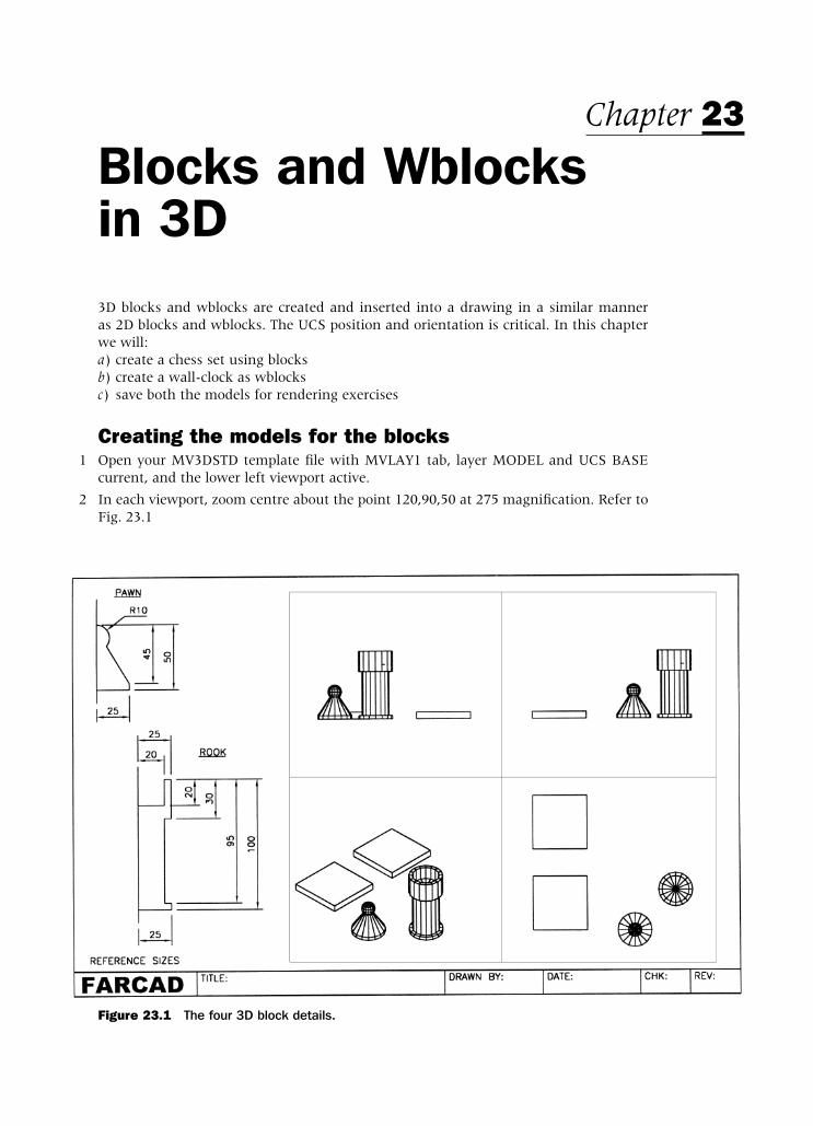
Blocks and Wblocks in 3D3D blocks and wblocks are created and inserted into a drawing in a similar manner as 2D blocks and wblocks. The UCS position and orientation is critical. In this chapterwe will:a) create a chess set using blocksb) create a wall-clock as wblocksc) save both the models for rendering exercises
Creating the models for the blocks1 Open your MV3DSTD template file with MVLAY1 tab, layer MODEL and UCS BASE
current, and the lower left viewport active.
2 In each viewport, zoom centre about the point 120,90,50 at 275 magnification. Refer toFig. 23.1
Chapter 23
Figure 23.1 The four 3D block details.
modelling with AutoCAD.qxd 17/06/2002 15:40 Page 151
3 With the lower left viewport active, create the following two 3D box objects:box1 box2
corner 0,0,0 0,120,0length 80 80width 80 80height 10 10rotation 0 0colour number 126 number 220
4 Restore UCS FRONT and make the upper right viewport active.
5 Draw a line with start point: 150,–10 and next point: @0,80
6 In paper space, zoom-window the top right viewport, then return to model space
7 a) Draw the pawn outline as a polyline from: 150,0 using your own design but with the‘overall’ sizes given as reference.
b) Set SURFTAB1 to 16c) With the REVOLVED SURFACE icon from the Surfaces toolbar, revolve the pawn
outline about the vertical line – full circle
d) The pawn colour is to be red
8 Still with UCS FRONT, draw a line with start point: 210,–10,–60 and next point: @0,120
9 a) Draw the rook outline as a polyline from: 210,0,–60 using the reference sizes givenor create your own design
b) Revolve the rook polyline about the vertical line (360 degs)c) The rook colour is to be red
10 Erase the two vertical lines
11 Restore UCS BASE and models displayed as Fig. 23.1.
Making the blocks1 With the lower left viewport active and UCS BASE, menu bar with Draw-Block-Make and:
prompt Block Definition dialogue boxrespond 1. enter name: SQ1
2. enter base point as X: 0; Y:0; Z: 03. pick Select objects and pick the green coloured box then right-click4. Objects: ensure Delete active5. Preview: Create icon from block geometry active6. enter description: FIRST SQUARE7. ensure insert units: millimeters (dialogue box as Fig. 23.2)8. pick OK
2 The green coloured square will be ‘made into a block’ and should disappear from thescreen due to respond 4
3 Using the Block Definition dialogue box, make the other three blocks using the samemethod as step 1 with the following information:
first second thirdname SQ2 PAWN ROOKinsertion pt 0,120,0 150,0,0 210,60,0object purple box 3D pawn 3D rookdescription SECOND SQUARE PAWN PIECE ROOK PIECE
4 Now erase the original polyline outlines which should be displayed
5 Activate the block definition dialogue box and scroll at name and the four created blocksshould be listed (PAWN, ROOK, SQ1, SQ2) in alphabetical order.
152 Modelling with AutoCAD 2002
modelling with AutoCAD.qxd 17/06/2002 15:40 Page 152

6 Note:a) The command line BLOCK <R> entry will display the Block Definition dialogue boxb) The command line entry –BLOCK <R> will allow block creation from the command line c) At the command line enter –BLOCK <R> and:
prompt Enter block name or [?] and enter: ? <R> – query optionprompt Enter block(s) to list and enter: * <R>prompt Text window with information about the four defined blocksrespond cancel the text window
Inserting the blocks1 Four ‘blank’ viewports should be displayed with MVLAY1 tab, UCS BASE, layer MODEL
and the 3D viewport active
2 Menu bar with Insert-Block and:prompt Insert dialogue boxrespond 1. scroll at name and pick SQ1
2. deactivate all on-screen prompts, i.e. no tick3. enter insertion point as X: 0; Y: 0; Z: 04. enter scale as X: 1; Y: 1; Z: 15. enter rotation as 06. dialogue box as Fig. 23.37. pick OK
and the green 3D box block will be displayed at the 0,0,0 insertion point
3 Repeat the Insert-Block sequence with:a) scroll and pick SQ2b) ensure on-screen prompts are offc) insertion point of X: 80; Y: 0; Z: 0d) scale of X: 1; Y: 1; Z: 1 and rotation: 0e) pick OK and the purple 3D box block displayed adjacent to the green 3D box
Block and Wblocks in 3D 153
Figure 23.2 Block Definition dialogue box for SQ1.
modelling with AutoCAD.qxd 17/06/2002 15:40 Page 153

4 Zoom centre about 320,320,100 at 700 in all viewports
5 With the 3D viewport active, complete the 64 square chess board using one of thefollowing methods:a) inserting each block SQ1 and SQ2b) multiple copy the two inserted boxesc) rectangular arrayd) note: I used multiple copy
6 At the command line enter –INSERT <R> and:prompt Enter block name and enter: PAWN <R>prompt Specify insertion point and enter: 40,120,10 <R>prompt Enter X scale factor and enter: 1 <R>prompt Enter Y scale factor and enter: 1 <R>prompt Specify rotation angle and enter: 0 <R>and the red pawn piece will be displayed on top of the left second row square
7 Now insert the ROOK full-size with 0 rotation at the insertion point of 40,40,10 usingeither the Insert dialogue box or the –INSERT command line entry.
8 a) Rectangular array the red pawn for 1 row and 8 columns, the column distance being80. Row distance is 0?
b) Copy the eight pawns from: 40,80,10 to: @0,400,0c) Multiple copy the rook from a base point of 40,40,10 to second points of: @560,0,0;
@0,560,0; @560,560,0
9 Taska) Alter the layout to display a three viewport configuration, remembering to make layer
VP currentb) set the viewpoints to display a 3D, top and front viewc) Change the colour of one set of prawns and rooks to blue. This may not be as simple
as you think. The inserted blocks must be exploded before the colour can be changed.Decide whether to use the PICKFIRST variable set to:i) 0: CHANGE at command line then pick the objectsii) 1: pick the objects then the Properties icon
d) re-centre the model in each viewport about 320,320,100 at 1100 magnification in the3D viewport and 700 in the other two
10 When complete, the layout should resemble Fig. 23.4 and should be saved asMODR2002\CHESS for the activity part of the chapter.
154 Modelling with AutoCAD 2002
Figure 23.3 The Insert dialogue box for SQ1.
modelling with AutoCAD.qxd 17/06/2002 15:40 Page 154

Creating the models for the Wblocks1 Open the MV3DSTD template file with MVLAY1 tab, UCS BASE and zoom centre about
125,0,100 at 300 magnification in all viewports. Refer to Fig. 23.5
2 The wblocks will be created using the WCS, so menu bar with Tools-New UCS-World
3 With the top right viewport active, layer MODEL current rotate the WCS about the Xaxis with menu bar sequence Tools-New UCS-X and enter 90 as the rotation angle
4 Create the three outlines for parts of a wall clock with:a) draw the body as lines using the 0,0,0 start point and the reference sizes given. Use
the Modify-Object-Polyline command to ‘convert’ the five lines into a single polylineobject
b) draw the face as an octagon circumscribed in a circle with centre at 90,90,0 and aradius of 40
c) draw the dial as a 30 radius circle, centre at 90,10,0
5 Draw the following three lines:a) line 1, start point: 150,0 next point: @0,0,40b) line 2, start point: 200,0 next point: @0,0,15c) line 3, start point: 250,0 next point: @0,0,8
6 The three wall clock components will be created as tabulated surface models, so setSURFTAB1 to 16
Block and Wblocks in 3D 155
Figure 23.4 The chess layout after the block insertions.
modelling with AutoCAD.qxd 17/06/2002 15:40 Page 155
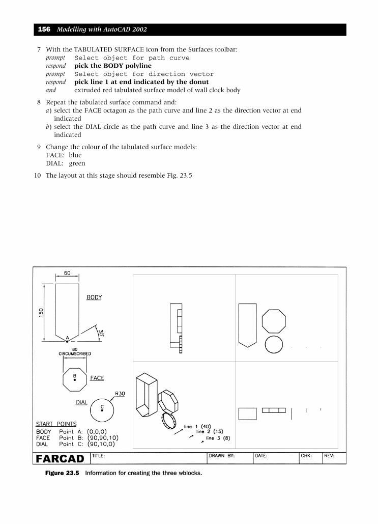
7 With the TABULATED SURFACE icon from the Surfaces toolbar:prompt Select object for path curverespond pick the BODY polylineprompt Select object for direction vectorrespond pick line 1 at end indicated by the donutand extruded red tabulated surface model of wall clock body
8 Repeat the tabulated surface command and:a) select the FACE octagon as the path curve and line 2 as the direction vector at end
indicated b) select the DIAL circle as the path curve and line 3 as the direction vector at end
indicated
9 Change the colour of the tabulated surface models: FACE: blueDIAL: green
10 The layout at this stage should resemble Fig. 23.5
156 Modelling with AutoCAD 2002
Figure 23.5 Information for creating the three wblocks.
modelling with AutoCAD.qxd 17/06/2002 15:40 Page 156
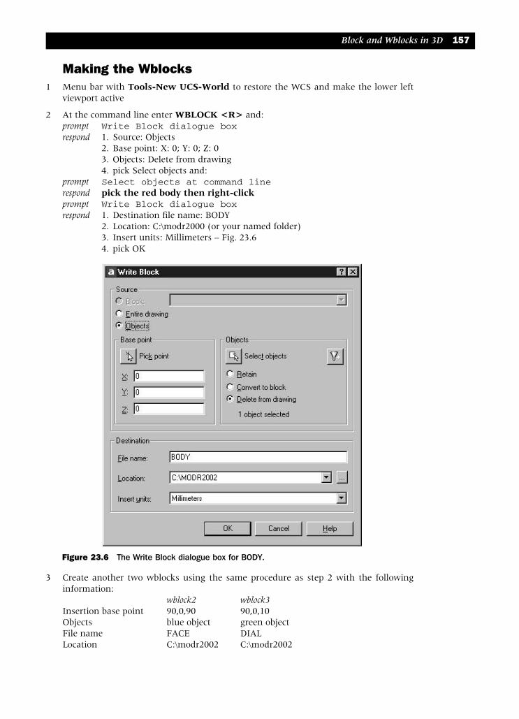
Making the Wblocks1 Menu bar with Tools-New UCS-World to restore the WCS and make the lower left
viewport active
2 At the command line enter WBLOCK <R> and:prompt Write Block dialogue boxrespond 1. Source: Objects
2. Base point: X: 0; Y: 0; Z: 03. Objects: Delete from drawing4. pick Select objects and:
prompt Select objects at command linerespond pick the red body then right-clickprompt Write Block dialogue boxrespond 1. Destination file name: BODY
2. Location: C:\modr2000 (or your named folder)3. Insert units: Millimeters – Fig. 23.64. pick OK
3 Create another two wblocks using the same procedure as step 2 with the followinginformation:
wblock2 wblock3Insertion base point 90,0,90 90,0,10Objects blue object green objectFile name FACE DIALLocation C:\modr2002 C:\modr2002
Block and Wblocks in 3D 157
Figure 23.6 The Write Block dialogue box for BODY.
modelling with AutoCAD.qxd 17/06/2002 15:40 Page 157

Inserting the three wblocks1 Menu bar with File-Close and pick No to save changes
2 Menu bar with File-New and ‘open’ your MV3DSTD template file with UCS BASE, layerMODEL, MVLAY1 tab and lower left viewport active
3 Restore the WCS
4 Menu bar with Insert-Block and:prompt Insert dialogue boxrespond pick Browseprompt Select Drawing File dialogue boxrespond 1. scroll and pick the C: drive
2. scroll and pick C:\modr2000 (or your named folder)3. pick BODY and note the preview4. pick Open
prompt Insert dialogue boxrespond 1. cancel the on-screen prompts
2. enter insertion point as X: 0; Y: 0; Z: 03. all scale factors 1 and rotation angle 04. pick OK
and the red body will be displayed at the 0,0,0 insertion point
5 Activate the Insert dialogue, select the Browse option and insert the other wblocks withthe following information:File name: FACE DIALInsertion point: 0,–40,130 0,–55,130X and Y scale: 1 1Rotation angle: 0 0
6 Zoom centre about the point 0,–30,80 at 200 magnification in all viewports – Fig. 23.7
7 Investigate the other layout tabs, centring the model using the following suggestion:Zoom-Extents then Zoom to scale 1.5
8 Hide and shade from the model tab and try 3D orbit
9 Save the model as MODR2002\WALL
158 Modelling with AutoCAD 2002
Figure 23.7 The completed wall clock created from inserted wblocks.
modelling with AutoCAD.qxd 17/06/2002 15:40 Page 158
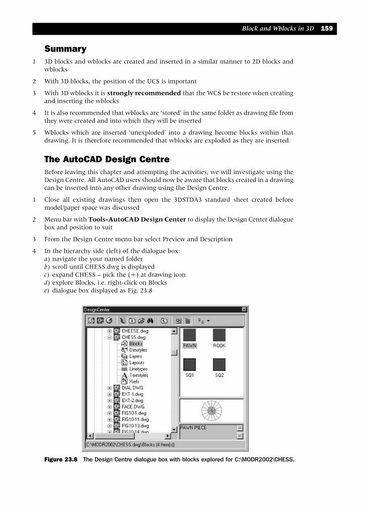
Summary1 3D blocks and wblocks are created and inserted in a similar manner to 2D blocks and
wblocks
2 With 3D blocks, the position of the UCS is important
3 With 3D wblocks it is strongly recommended that the WCS be restore when creatingand inserting the wblocks
4 It is also recommended that wblocks are ‘stored’ in the same folder as drawing file fromthey were created and into which they will be inserted
5 Wblocks which are inserted ‘unexploded’ into a drawing become blocks within thatdrawing. It is therefore recommended that wblocks are exploded as they are inserted.
The AutoCAD Design CentreBefore leaving this chapter and attempting the activities, we will investigate using theDesign Centre. All AutoCAD users should now be aware that blocks created in a drawingcan be inserted into any other drawing using the Design Centre.
1 Close all existing drawings then open the 3DSTDA3 standard sheet created beforemodel/paper space was discussed
2 Menu bar with Tools-AutoCAD Design Center to display the Design Center dialoguebox and position to suit
3 From the Design Centre menu bar select Preview and Description
4 In the hierarchy side (left) of the dialogue box:a) navigate the your named folderb) scroll until CHESS.dwg is displayedc) expand CHESS – pick the (+) at drawing icond) explore Blocks, i.e. right-click on Blockse) dialogue box displayed as Fig. 23.8
Block and Wblocks in 3D 159
Figure 23.8 The Design Centre dialogue box with blocks explored for C:\MODR2002\CHESS.
modelling with AutoCAD.qxd 17/06/2002 15:40 Page 159

5 Right-click the SQ1 icon from the Design Center palette and:prompt Shortcut menurespond pick Insert blockprompt Insert dialogue boxwith SQ1 named and dialogue box as beforerespond cancel the dialogue box and the Design Center
6 This exercise was to demonstrate that the Design Center can be used to insert ANY blockfrom any drawing into any other drawing
AssignmentsTwo activities have been included for you to attempt, one involving the partiallycompleted chess set, and the other using two previously saved drawings, one of whichwill be inserted as a wblock into the other.
ACTIVITY 15: CHESS SET1 Recall the drawing CHESS saved earlier in this chapter to display the 64 square chess
board with the two sets of red and blue pawns and rooks.
2 Design the other chess pieces – KNIGHT, BISHOP, KING and QUEEN using the samemethod as the worked example:a) draw the outline as a polylineb) use the revolved surface command to create the piece as a 3D surface modelc) the actual shape of the pieces is at your discretion.d) the information given in the Activity 15 drawing is for reference purposes onlye) ensure that your start point for the outline is known – it will be useful as the block
insertion point
3 Create a block of each created piece
4 Insert the created blocks onto the chess board
5 Complete the chess set layout, remembering to change the colours of the pieces to redand blue as appropriate.
6 Save as MODR2002\CHESS.
7 Investigate the various shade options with the completed model
8 Note: the model layout displayed in activity 15 was produced by Craig Matthewman. Craigwas a full-time student on the HNC CADD course at Motherwell College and his designwas interesting. He gave his permission for the layout to be included as an activity.
ACTIVITY 16: Palace of Queen NEFERSAYDY built by MACFARAMUS.
MACFARAMUS was last encountered building the palace for queen NEFERSAYDY.Unfortunately this palace was to be built on a flat topped hill and you have to create thelayout using an existing drawing and inserting another drawing into it as a wblock.
1 Open the drawing MODR2002\HILL of the edge surface model created as activity 13
2 Insert the wblock drawing file MODR2002\PALACE of the 3D objects created as activity 14
3 The palace has to be positioned at the centre point of the hill top, and the coordinatesof this point as 0,0,100. This is the only help given.
4 Optimise all the layout tabs for maximum effect.
5 When complete save the layout as MODR2002\HILLPAL
160 Modelling with AutoCAD 2002
modelling with AutoCAD.qxd 17/06/2002 15:40 Page 160

Dynamic viewingDynamic viewing is a powerful (yet underused) command which is very useful with 3Dmodelling as it allows models to be viewed from a perspective viewpoint. The commandalso allows objects to be ‘cut-away’ enabling the user to ‘see inside’ models. Dynamicviewing has its own terminology which is obvious when you are familiar with thecommand, but can be confusing to new users.
The basic concept of dynamic viewing is that the user has a CAMERA which ispositioned at a certain DISTANCE from the model – called the TARGET. The user islooking through the camera lens at the model and can ZOOM in/out as required. Theviewing direction is from the camera lens to a TARGET POINT on the model. Thecamera can be moved relative to the stationary target, and both the camera and targetcan be turned relative to each other. The target can also be TWISTED relative to thecamera. Two other concepts which the user will encounter with the dynamic viewcommand are the slider bar and the perspective icon. The slider bar allows the userto ‘scale’ the variable which is current, while the perspective icon is displayed when theperspective view is ‘on’.
Figure 24.1(A) displays the various dynamic view concepts of: a) the basic terminologyb) the slider barc) the perspective icon
Chapter 24
Figure 24.1 Dynamic view terminology and AutoCAD’s DVIEWBLOCK ‘house’.
modelling with AutoCAD.qxd 17/06/2002 15:40 Page 161

The dynamic view command has eleven options, these being:
CAmera,TArget,Distance,POints,Pan,Zoom,TWist,CLip,Hide,Off,Undo
The option required is activated by entering the CAPITAL letters at the command line,e.g. CA for the camera option, TW for twist etc.
We will investigate the dynamic view command with two examples:
1 using AutoCAD’s dynamic view ‘house’
2 with a previously created and saved model
Note1 Dynamic view is a model space concept, and cannot be used in paper space.
2 Dynamic view is viewport independent, i.e. if the command is used in a specificviewport, the model display in the other viewports will not be affected.
3 The command is activated by entering DVIEW <R> at the command line
Example 1 – AutoCAD’s ‘house’AutoCAD has a ‘drawing’ – actually a type of block – which can be used as an interactiveaid with the dynamic view command. We will use this house block to demonstrate someof the options so:
1 Close any existing drawings and start a new metric drawing from scratch and refer toFig. 24.1(B)
2 At the command line enter DVIEW <R> and:prompt Select objects or <use DVIEWBLOCK>respond <RETURN> i.e. accept the DVIEWBLOCK default
a) prompt Enter option[Camera/Target/Distance/Points/Pan/Zoom/Twist/Clip/Hide/Off/Undo]
and some coloured lines appear on the screenenter Z <R> – the zoom optionprompt slider bar with scale displayed at top of screenand Specify zoom scale factorenter 0.5 <R>and full plan view of house – fig(a)
b) prompt Enter option [CAmera/TArget/etcenter CA <R> – the camera optionprompt ghost image of house which moves as mouse movedand Specify camera location or enter angle from XY plane enter 30 <R>prompt Specify camera location or enter angle in XY plane from
X axisenter 30 <R>and 3D view of house – fig(b)
c) prompt Enter option [CAmera/TArget/etcenter H <R> – the hide optionand house displayed with hidden line removal – fig(c)
162 Modelling with AutoCAD 2002
modelling with AutoCAD.qxd 17/06/2002 15:40 Page 162

d) prompt Enter option [CAmera/TArget/etcenter CL <R> – the clip optionprompt Enter clipping option [Back/Front/Off]enter F <R> – the front clip optionprompt Specify distance from target or [set to Eye(camera)/ON/OFF]enter 40 <R>prompt Enter option [CAmera/TArget/etcenter H <R> – the hide optionand house displayed ‘cut-away’ similar to fig(d)
e) enter U <R> – undoes the hide effect of (d)enter U <R> – undoes the clip effect of (d)enter U <R> – undoes the hide effect of (c)and leave house with Camera option displayedand command prompt line optionsthen read the explanation before proceeding
Explanation of the dynamic view commandDynamic view is an interactive command and the various options can be used one afterthe other. The undo (U) option will undo the last option performed, and can be usedrepeatedly until all the options entered have been ‘undone’. Some of the options havebeen used to demonstrate how the command is used, these options being zoom, camera,clip, hide and undo. The hide option is very useful as it allows the model to be displayedwhen other options have been entered, and removes the ‘ambiguity’ effect from themodel. The command can be used with all 3D models, i.e. extruded, wire-frame, surfaceand solid. The command is also viewport independent, i.e. it can be used in anyviewport without affecting the display in other viewports. The AutoCAD ‘house’ is a user-reference, and if a model is displayed on the screen, this model will assume the houseorientation when the dynamic view command is completed. This will be investigatedduring the next example.
Dynamic viewing 163
Figure 24.2 The various DVIEW options with DVIEWBLOCK – AutoCAD’s house.
modelling with AutoCAD.qxd 17/06/2002 15:40 Page 163

The house displayed on the screen has been left with the Camera option with enteredangles of 30 and 30. We will continue with the screen display and investigate the otherdynamic view options. This means that you have to enter the various options and valuesas prompted.
Refer to Fig. 24.2 which displays one entry (with hide) from the exercises which follow.
CAmera1 This option is used to direct the camera at the target and the camera can be ‘tilted’
relative to the target. These are two angle prompts:prompt 1 angle in the XY plane, between –90degs and +90degsprompt 2 angle from the XY plane, between –180degs and +180degs
2 The angles can be:a) toggled using the ghost image as a guideb) entered directly from the keyboard
3 Using the CAmera option enter the following angle values:angle in XY plane angle from XY plane
a) 35 35b) 35 –35c) –35 35d) –35 –35
4 The option can be considered similar to VPOINT-ROTATE
5 When all the above entries have been completed, return the camera angles to the original30 and 30, but do not exit the command.
TArget1 This option allows the target (the model) to be tilted relative to the camera. The two
angle prompts are the same as the camera option:prompt 1 angle in the XY planeprompt 2 angle from the XY plane
2 The angles can be toggled or entered from the keyboard
3 Using the TArget option enter the following angle values:angle in XY plane angle from XY plane
a) 35 35b) 35 –35c) –35 35d) –35 –35
4 The option can be used to give the same effect as the camera option, but it should beremembered that the camera and target are being ‘tilted’ in the ‘opposite sense’ to each other
5 When all angles have been entered, restore the camera to angles of 30 and 30, but donot exit the command.
TWist1 A very useful option as it allows the ‘plane’ on which the target is ‘resting’ to be twisted
through an entered angle. This angle can be positive or negative and have values between0 and 360degs
2 The prompt with this option is: Specify new view twist angle
3 The result of the option is dependent on the CAmera/Target angles
164 Modelling with AutoCAD 2002
modelling with AutoCAD.qxd 17/06/2002 15:40 Page 164

4 Using the TWist option enter angle values of:a) 35 b) –35 c) 180 d) –90
5 This is one of the few AutoCAD commands which allows models to be ‘flipped’ over by180degs.
6 When the four twist angles have been viewed with the hide effect, restore the originaltwist angle of 0, with the camera options of 30 and 30. Do not exit the command.
CLip1 The clip option of the dynamic view command is probably of the most useful of all the
options, as it allows models to be ‘cut-away’, thus allowing the user to ‘see inside’ the model.
2 The user selects a (F)ront or (B)ack clip and then decides on the clip distance either:a) using the slider barb) entering a value at the command line
3 The result of the clip option is dependent on the CAmera/TArget angles as well as the‘size’ of the model on the screen
4 With the CAmera angles set to 30 and 30, activate the front clip option and move theslider bar until the ghost image displays a clip effect then right-click
5 When the clip option attempts are complete, undo the various effects with U <R> untilthe house is again displayed with the CAmera settings of 30 and 30.
POints1 This option allows the model (the target) to be viewed from a specific ‘stand point’, the
user looking at a specific point on the target.
2 Two sets of coordinates need to be specified:a) the target point coordinates to be looked atb) the coordinates of the camera – the user
3 The coordinate entries can be absolute or relative
4 When this option is used, the PAn option is also usually needed
5 The result does not depend on the CAmera or TArget options
6 Use the Point option with the following entries:target point camera point
a) 0,0,0 1,0,0b) 0,0,0 0,1,0c) 0,0,0 0,0,1d) 0,0,0 1,1,0e) 0,0,0 1,0,1f) 0,0,0 1,1,1g) 1,2,3 0,0,0h) 0,0,0 1,2,3
7 The option is similar to the VPOINT-VECTOR command.
8 When all the points entries have been entered, restore the camera angles of 30 and 30,but do not exit the command.
Dynamic viewing 165
modelling with AutoCAD.qxd 17/06/2002 15:40 Page 165

Distance1 Alters the distance between the camera and the target
2 The distance can be:a) entered as a value from the command lineb) toggled using the slider bar
3 With the distance option, enter some values e.g.:a) 1000 b) 1500 c) 2500 d) 5000
4 The distance option introduces true perspective to the model
5 When the distance option has been used, and the command is exited, the zoomcommand cannot be used.
6 Restore the original CAmera option of 30 and 30
Zoom1 This option does what you would expect – it ‘zooms the model’
2 The zoom factor can be:a) entered as a value from the keyboardb) toggled using the slider bar
3 Try some zoom entries e.g.:a) 1 b) 0.75 c) 0.5 d) 0.25
4 Restore the original CAmera effect (30,30) and use the zoom option with a 0.5 scale factorthree times.
Pan1 This option is similar to the AutoCAD PAN command, but the ‘real-time’ pan effect is
not available.
2 The user selects (or enters) the pan displacement
Hide1 Will display the model with a hide effect
2 Removes any ambiguity
Undo1 Entering U <R> will undo the last option of the DVIEW command
2 Can be used repetitively until all the option entries have been undone
eXit1 Entering X <R> will end the dynamic view command and a blank screen will be
returned
2 The blank screen is because we did not have any model displayed, the AutoCAD ‘house’being a visual aid indicating what any model would ‘look like’
3 With ‘real models’, the model orientation will be similar to the ‘house’ orientation whenthe DVIEW command has been exited, as will now be investigated.
4 If the DVIEW command is still active, enter X <R>
5 This first exercise is now complete.
166 Modelling with AutoCAD 2002
modelling with AutoCAD.qxd 17/06/2002 15:40 Page 166

Example 2 – an 3D modelIn this example we will use the dynamic view command with a previously created model.
1 Open the ruled surface model MODR2002\ARCHES created during chapter 16 with UCSBASE, layer MODEL. Re-centre the model about the point 50,10,75 at 150 mag.
2 Make the upper left viewport active and refer to Fig. 24.3
3 At the command line enter DVIEW <R> and:prompt Select objects or use <DVIEWBLOCK> respond <RETURN>prompt AutoCAD’s house as an ‘end view’ in the active viewportand dynamic view optionsenter CA <R>prompt Angle from XY plane and enter: –20 <R>prompt Angle in XY plane and enter: 30 <R>prompt dynamic view options and enter: X <R>
4 The model will be displayed with house CAmera configuration as fig(b) with hide
5 With the top right viewport active, enter DVIEW <R> at the command line and:prompt Select objects or use <DVIEWBLOCK>respond window the model then right-clickprompt dynamic view optionsenter TW <R>prompt Specify view twist angle and enter: –90 <R>prompt dynamic view options and enter: X <R>and Model displayed with new twist as fig(c)
Dynamic viewing 167
Figure 24.3 Dynamic view example 2 using MODR2002\ARCHES.
modelling with AutoCAD.qxd 18/06/2002 11:23 Page 167

6 Use the dynamic view command in the lower viewports with the following entries:lower left lower rightoptions: TArget options: CAmeraangles: 40 and –30 angles: 30 and 30options: CLip, Front options: TWist, angle: 180distance: 10 options: CLip, Front, Distance: 15options: X options: Xfig(d) fig(e)
7 Note: if the clip-front distances do not give the exact same effect as Fig. 24.3 it could beas a result of your model having a different zoom effect from mine.
8 Save the drawing if required, but we will not refer to this exercise again.
Summary1 The dynamic view command is viewport specific, i.e. it only affects the active viewport
2 The command has several useful options:a) CAmera, TArget: similar to VPOINT rotateb) TWist: allows models to be ‘inverted’c) Distance: introduces true perspectived) CLip: useful to ‘see inside’ models
3 The command can only be activated with DVIEW <R> at the command line
4 The command can be used:a) directly on modelsb) interactively using AutoCAD’s house
5 The command is used relative to the WCS – observe the prompt line when the commandis activated.
AssignmentNo specific activity, but investigate DVIEW with some previously created models.
168 Modelling with AutoCAD 2002
modelling with AutoCAD.qxd 17/06/2002 15:40 Page 168

Viewport specificlayersWhen layers are used with multiple viewports they are generally GLOBAL, i.e. what isdrawn on a layer in one viewport will be displayed in the other viewports. This is quiteacceptable for creating models but is unacceptable for certain other concepts, e.g. addingdimensions to a model, sectioning the model, obtaining a true shape etc. If dimensions(for example) have to be added to a model in a multi-view layout, then these dimensionsshould only be visible in the active viewport. This is also true for true shapes and sections.
In this chapter we will investigate how to create and use viewport specific layers byadding dimensions to an existing model.
Note1 Remember that dimensioning is a 2D concept, the result depending on the position and
orientation of the UCS. Think back to when we dimensioned the 3D wire-frame model.
2 In later chapters we will use viewport specific layers to extract sections and true shapesfrom solid models
3 Although dimensioning is being used to demonstrate using viewport specific layers, laterchapters will introduce the user to other methods of dimensioning models.
Global layers1 Open the 3D faced model MODR2002\CHEESE from chapter 14 and refer to Fig. 25.1
2 With the MVLAY1 tab current, UCS BASE, lower right viewport active make layer DIMcurrent and display the Dimension toolbar
3 Select the LINEAR DIMENSION icon from the Dimension toolbar and dimension lines1–2 and 1–3.
4 Make the upper right viewport active and restore UCS FRONT
5 Linear dimension line a-b and baseline dimension lines a–c and a–d.
6 The five dimensions will be displayed in all four viewports due to the GLOBAL natureof layer DIM. Fig. 25.1(a) displays the five dimensions as displayed in the 3D viewport.
7 Now erase the five dimensions and restore UCS BASE
Chapter 25
modelling with AutoCAD.qxd 17/06/2002 15:40 Page 169
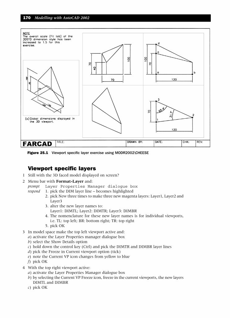
Viewport specific layers1 Still with the 3D faced model displayed on screen?
2 Menu bar with Format-Layer and:prompt Layer Properties Manager dialogue boxrespond 1. pick the DIM layer line – becomes highlighted
2. pick New three times to make three new magenta layers: Layer1, Layer2 andLayer3
3. alter the new layer names to:Layer1: DIMTL; Layer2: DIMTR; Layer3: DIMBR
4. The nomenclature for these new layer names is for individual viewports, i.e. TL: top left; BR: bottom right; TR: top right
5. pick OK
3 In model space make the top left viewport active and:a) activate the Layer Properties manager dialogue boxb) select the Show Details optionc) hold down the control key (Ctrl) and pick the DIMTR and DIMBR layer linesd) pick the Freeze in Current viewport option (tick)e) note the Current VP icon changes from yellow to bluef) pick OK
4 With the top right viewport active:a) activate the Layer Properties Manager dialogue boxb) by selecting the Current VP Freeze icon, freeze in the current viewports, the new layers
DIMTL and DIMBRc) pick OK
170 Modelling with AutoCAD 2002
Figure 25.1 Viewport specific layer exercise using MODR2002\CHEESE
modelling with AutoCAD.qxd 17/06/2002 15:40 Page 170
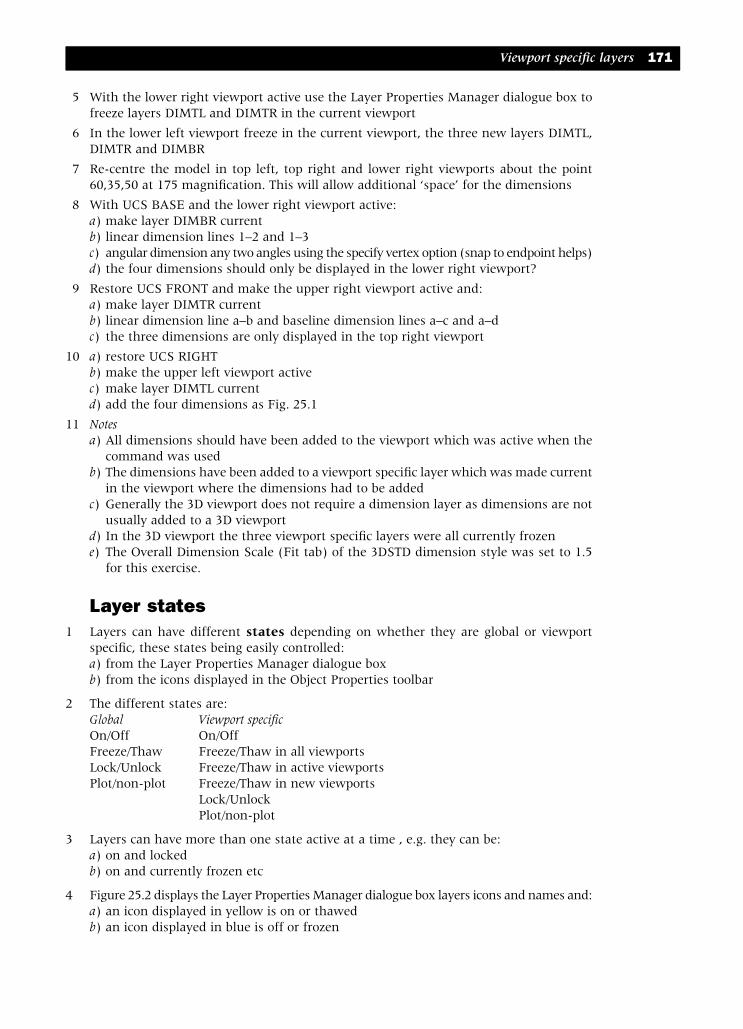
5 With the lower right viewport active use the Layer Properties Manager dialogue box tofreeze layers DIMTL and DIMTR in the current viewport
6 In the lower left viewport freeze in the current viewport, the three new layers DIMTL,DIMTR and DIMBR
7 Re-centre the model in top left, top right and lower right viewports about the point60,35,50 at 175 magnification. This will allow additional ‘space’ for the dimensions
8 With UCS BASE and the lower right viewport active:a) make layer DIMBR currentb) linear dimension lines 1–2 and 1–3c) angular dimension any two angles using the specify vertex option (snap to endpoint helps)d) the four dimensions should only be displayed in the lower right viewport?
9 Restore UCS FRONT and make the upper right viewport active and:a) make layer DIMTR currentb) linear dimension line a–b and baseline dimension lines a–c and a–dc) the three dimensions are only displayed in the top right viewport
10 a) restore UCS RIGHTb) make the upper left viewport activec) make layer DIMTL currentd) add the four dimensions as Fig. 25.1
11 Notesa) All dimensions should have been added to the viewport which was active when the
command was usedb) The dimensions have been added to a viewport specific layer which was made current
in the viewport where the dimensions had to be addedc) Generally the 3D viewport does not require a dimension layer as dimensions are not
usually added to a 3D viewportd) In the 3D viewport the three viewport specific layers were all currently frozene) The Overall Dimension Scale (Fit tab) of the 3DSTD dimension style was set to 1.5
for this exercise.
Layer states1 Layers can have different states depending on whether they are global or viewport
specific, these states being easily controlled:a) from the Layer Properties Manager dialogue boxb) from the icons displayed in the Object Properties toolbar
2 The different states are:Global Viewport specificOn/Off On/OffFreeze/Thaw Freeze/Thaw in all viewportsLock/Unlock Freeze/Thaw in active viewportsPlot/non-plot Freeze/Thaw in new viewports
Lock/UnlockPlot/non-plot
3 Layers can have more than one state active at a time , e.g. they can be:a) on and lockedb) on and currently frozen etc
4 Figure 25.2 displays the Layer Properties Manager dialogue box layers icons and names and:a) an icon displayed in yellow is on or thawedb) an icon displayed in blue is off or frozen
Viewport specific layers 171
modelling with AutoCAD.qxd 17/06/2002 15:40 Page 171
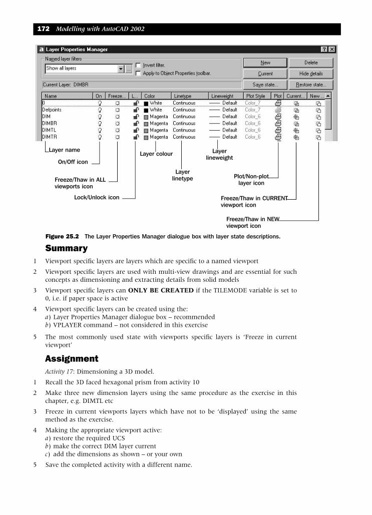
Summary1 Viewport specific layers are layers which are specific to a named viewport
2 Viewport specific layers are used with multi-view drawings and are essential for suchconcepts as dimensioning and extracting details from solid models
3 Viewport specific layers can ONLY BE CREATED if the TILEMODE variable is set to0, i.e. if paper space is active
4 Viewport specific layers can be created using the:a) Layer Properties Manager dialogue box – recommendedb) VPLAYER command – not considered in this exercise
5 The most commonly used state with viewports specific layers is ‘Freeze in currentviewport’
AssignmentActivity 17: Dimensioning a 3D model.
1 Recall the 3D faced hexagonal prism from activity 10
2 Make three new dimension layers using the same procedure as the exercise in thischapter, e.g. DIMTL etc
3 Freeze in current viewports layers which have not to be ‘displayed’ using the samemethod as the exercise.
4 Making the appropriate viewport active:a) restore the required UCSb) make the correct DIM layer currentc) add the dimensions as shown – or your own
5 Save the completed activity with a different name.
172 Modelling with AutoCAD 2002
Figure 25.2 The Layer Properties Manager dialogue box with layer state descriptions.
Layer name
On/Off icon
Freeze/Thaw in ALLviewports icon
Freeze/Thaw in CURRENTviewport icon
Freeze/Thaw in NEWviewport icon
Lock/Unlock icon
Layer colour
Layerlinetype
Layerlineweight
Plot/Non-plotlayer icon
modelling with AutoCAD.qxd 17/06/2002 15:40 Page 172
Shading and 3D orbitShading and 3D orbit have been used in previous chapters without any discussion. Inthis chapter we will investigate both topics in greater detail.
ShadingShading allows certain models to be displayed on the screen as a more realistic colouredimage. The models which can be shaded (and rendered) are 21/2D extruded models, 3Dobjects, 3D surface models and solid models. We will use some previously created 3Dsurface models to investigate the topic.
1 Open the ruled surface model MODR2002\ARCHES from chapter 14
2 Make the model tab active and restore UCS BASE. Any layer can be active
3 a) Menu bar with View-Hide to display the model with hidden line removal. Note the2D icon is still displayed
b) Menu bar with View-Regen to restore original model
4 a) Menu bar with View-Shade-Hidden and the model will be displayed with hiddenline removal, but note the coloured 3D icon with X-axis red, Y-axis green and Z-axisblue
b) Menu bar with View-Regen and model is unchangedc) Menu bar with View-Shade-3D Wireframe and the model will be displayed without
hidden line removal, but the coloured 3D icon is still displayedd) Menu bar with View-Shade-2D Wireframe to restore the original model with the
2D icon
5 Using the menu bar sequence View-Shade, activate the four shade options returning the display to 3D Wireframe before activating the next option. Note the difference inthe shading between the Flat and Gouraud options, evident at the arch curved ‘shoulders.
Explanation of the shade optionsActivating SHADE from the View pull-down menu allows the user access to sevenoptions. These options allow models to be displayed as shaded/wireframe images asfollows:
1 2D Wireframe: The model is displayed with the boundaries as lines and curves with the ‘normal’ 2Dicon. This option is generally used to restore shaded models to their original appearance.
2 3D Wireframe:Models are displayed as lines and curves for their boundaries but with a coloured 3Dicon. When used, this option restores shaded models to their original appearance butretains the coloured 3D icon.
Chapter 26
modelling with AutoCAD.qxd 17/06/2002 15:40 Page 173

3 Hidden:Displays models with hidden line removal and displays the coloured 3D icon. The REGENcommand will not work when this option has been used, and models are restored totheir original appearance with either the 2D Wireframe or 3D Wireframe options.
4 Flat Shaded:Models are shaded between their polygon mesh faces and appear flatter and less smooththan the Gouraud shaded models. Any materials (later chapter) which have been appliedare also displayed flat shaded
5 Gouraud Shaded:Models are shaded with the edges between the polygon mesh faces smoothed. Thisoption gives models a realistic appearance. Added materials are also Gouraud shaded.
6 Flat Shaded, Edges On:Models are flat shaded with the wireframe showing through the shade effect
7 Gouraud Shaded, Edges On:Models displayed with the Gouraud shading effect and the wireframe shows through
8 General:a) Both the Flat and Gouraud shading options display the coloured 3D iconb) The Flat and Gouraud shading use the 2D wireframe or the 3D Wireframe options to
restore the model to its original appearancec) The REDRAW/REGEN/REGENALL commands cannot be used if the View-Shade
sequence is activatedd) If HIDE <R> is entered from the command line to display any model with hidden
line removal, then REGEN can be used.
This completes the shading part of the chapter. Ensure that the ARCHES drawing is stilldisplayed in the model tab for the 3D orbit exercise.
3D orbitThe 3D orbit command (introduced in AutoCAD Release 2000) allows real-time 3Drotation, the user controlling this rotation with the pointing device. The basic conceptis that you are viewing the model (the target) with a camera (the user), the targetremaining stationary while the camera moves around the target. The opposite effect isdisplayed on the screen, i.e. the models appears to ‘rotate’.
The 3D orbit concept has its own terminology, the most common being the arcball andicons – Fig. 26.1.
1 Arcball: is a circle with smaller circles at the quadrants
2 Icons: which alter in appearance dependent on were the pointing device is positionedrelative to the arcball
3 Click and drag: the term for holding down the left button of the mouse and moving themouse to give rotation of the model
4 Roll: a type of rotation when the icon is outside the arcball. It is a rotation about an axisthrough the centre of the arcball perpendicular to the screen.
174 Modelling with AutoCAD 2002
modelling with AutoCAD.qxd 17/06/2002 15:40 Page 174

Using 3D orbit1 The ARCHES model should still be displayed in Model tab
2 Pick the 3D Orbit icon from the Standard toolbar and:prompt Arcball displayedrespond a) hold down the left mouse button
b) move the mouse about the screenc) release the mouse buttond) practice this hold down, move, release and note the movement of the modele) press ESC to end command
3 Restore the model to its original viewpoint with U <R>
4 Menu bar with View-Shade-Gouraud Shaded
5 At the command line enter 3DORBIT <R> and:prompt Arcball displayedrespond right-click prompt Shortcut menurespond pick Moreprompt cascade shortcut menu – Fig. 26.2respond pick Continuous Orbitprompt continuous icon displayedrespond 1. move mouse slightly then leave it alone
2. model displayed shaded with continuous rotation3. use the mouse left button to alter the rotation 4. practice the continuous rotation5. right-click and pick Exit
6 Restore the model to the original orientation with U <R>
Shading and 3D orbit 175
Figure 26.1 The basic 3D orbit terminology.
modelling with AutoCAD.qxd 17/06/2002 15:40 Page 175
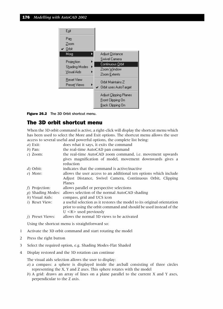
The 3D orbit shortcut menuWhen the 3D orbit command is active, a right-click will display the shortcut menu whichhas been used to select the More and Exit options. The shortcut menu allows the useraccess to several useful and powerful options, the complete list being:a) Exit: does what it says, it exits the commandb) Pan: the real-time AutoCAD pan commandc) Zoom: the real-time AutoCAD zoom command, i.e. movement upwards
gives magnification of model, movement downwards gives areduction
d) Orbit: indicates that the command is active/inactivee) More: allows the user access to an additional ten options which include
Adjust Distance, Swivel Camera, Continuous Orbit, ClippingPlanes
f) Projection: allows parallel or perspective selectionsg) Shading Modes: allows selection of the normal AutoCAD shadingh) Visual Aids: compass, grid and UCS iconi) Reset View: a useful selection as it restores the model to its original orientation
prior to using the orbit command and should be used instead of theU <R> used previously
j) Preset Views: allows the normal 3D views to be activated
Using the shortcut menu is straightforward so:
1 Activate the 3D orbit command and start rotating the model
2 Press the right button
3 Select the required option, e.g. Shading Modes-Flat Shaded
4 Display restored and the 3D rotation can continue
The visual aids selection allows the user to display:a) a compass: a sphere is displayed inside the arcball consisting of three circles
representing the X, Y and Z axes. This sphere rotates with the modelb) A grid: draws an array of lines on a plane parallel to the current X and Y axes,
perpendicular to the Z axis.
176 Modelling with AutoCAD 2002
Figure 26.2 The 3D Orbit shortcut menu.
modelling with AutoCAD.qxd 17/06/2002 15:40 Page 176

The clipping planesThe clipping plane options in 3D orbit are similar to the clip option of the DVIEWcommand, i.e. the clipping plane is an invisible plane set by the user. Parts of the modelcan be clipped, i.e. ‘cut-away’ relative to this clipping plane. To demonstrate the option:
1 Restore the model to its original orientation
2 Start the model rotating with the 3D orbit command
3 Activate the shortcut menu and select the Hidden shading mode
4 Activate the shortcut menu and select More-Adjust Clipping Plane and:prompt Adjust Clipping Plane dialogue boxrespond 1. pick the Adjust Front Clipping icon
2. drag the datum plane downwards – Fig. 26.3(a)3. right-click and close
5 Continue with the 3D orbit and the model will be rotated with a front clip effect – Fig. 26.3(b)
6 When you are satisfied with the display:a) right-click and reset viewb) right-click and exit
7 The model should be restored to its original orientation
8 Try this clipping plane option a few times. It is relatively easy to use.
Shading and 3D orbit 177
Figure 26.3 Using the More-Adjust Clipping Planes option of 3D orbit.
Adjust Front Clipping
(a) (b)
modelling with AutoCAD.qxd 17/06/2002 15:40 Page 177
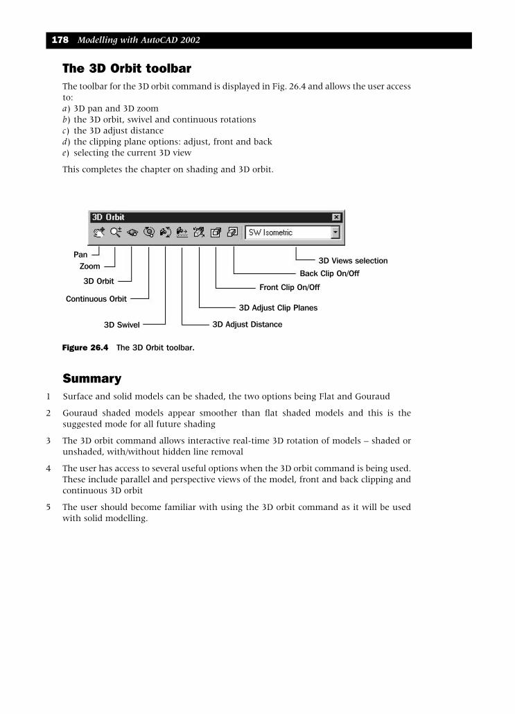
The 3D Orbit toolbarThe toolbar for the 3D orbit command is displayed in Fig. 26.4 and allows the user accessto:a) 3D pan and 3D zoomb) the 3D orbit, swivel and continuous rotationsc) the 3D adjust distanced) the clipping plane options: adjust, front and backe) selecting the current 3D view
This completes the chapter on shading and 3D orbit.
Summary1 Surface and solid models can be shaded, the two options being Flat and Gouraud
2 Gouraud shaded models appear smoother than flat shaded models and this is thesuggested mode for all future shading
3 The 3D orbit command allows interactive real-time 3D rotation of models – shaded orunshaded, with/without hidden line removal
4 The user has access to several useful options when the 3D orbit command is being used.These include parallel and perspective views of the model, front and back clipping andcontinuous 3D orbit
5 The user should become familiar with using the 3D orbit command as it will be usedwith solid modelling.
178 Modelling with AutoCAD 2002
Figure 26.4 The 3D Orbit toolbar.
PanZoom
3D Orbit
Continuous Orbit
3D Swivel
3D Views selection
Back Clip On/Off
Front Clip On/Off
3D Adjust Clip Planes
3D Adjust Distance
modelling with AutoCAD.qxd 17/06/2002 15:40 Page 178
Introduction to solidmodellingThree dimensional modelling with computer-aided draughting and design (CADD) canbe considered as three categories:
• wire-frame modelling
• surface modelling
• solid modelling
We have already created wire-frame and surface models and will now concentrated onhow solid models are created.
This chapter will summarise the three model types.
Wire-frame modelling1 Wire-frame models are defined by points and lines and are the simplest possible
representation of a 3D component. They may be adequate for certain 3D modelrepresentation and require less memory than the other two 3D model types, but wire-frame models have several limitations:a) Ambiguity: it is difficult to know how a wire-frame model is being viewed, i.e. from
above or from below?b) No curved surfaces: while curves can be added to a wire-frame model as arcs or trimmed
circles, an actual curved surface cannot. Lines may be added to give a ‘curved effect’but the computer does not recognise these as being part of the model.
c) No interference: as wire-frame models have no surfaces, they cannot detect interferencebetween adjacent components. This makes then unsuitable for kinematic displays,simulations etc.
d) No physical properties: mass, volume, centre of gravity, moments of inertia, etc. cannotbe calculated
e) No shading: as there are no surfaces, a wire-frame model cannot be shaded or rendered.f) No hidden line removal: as there are no surfaces, it is not possible to display the model
with hidden line removal.
2 AutoCAD 2002 allows wire-frame models to be created.
Chapter 27
modelling with AutoCAD.qxd 17/06/2002 15:40 Page 179

Surface modelling1 A surface model is defined by points, lines and faces. A wire-frame model can be
‘converted’ into a surface model by adding these ‘faces’. Surface models have severaladvantages when compared to wire-frame models, some of these being:a) Recognition and display of curved profilesb) Shading, rendering and hidden line removal are all possible, i.e. no ambiguityc) Recognition of holes
2 Surface models are suited to many applications but they have some limitations whichinclude:a) No physical properties: other than surface area, a surface model does not allow the
calculation of mass, volume, centre of gravity, moments of inertia, etc.b) No detail: a surface model does not allow section detail to be obtained.
3 Several types of surface model can be generated including:a) plane and curved swept surfacesb) swept area surfacesc) rotated or revolved surfacesd) splined curve surfacese) nets or meshes
4 AutoCAD 2002 allows surface models of these types to be created.
Solid modelling1 A solid model is defined by the volume the component occupies and is thus a real 3D
representation of the component. Solid modelling has many advantages which include:a) Complete physical properties of mass, volume, centre of gravity, moments of inertia, etc.b) Dynamic properties of momentum, angular momentum, radius of gyration, etc.c) Material properties of stress-straind) Full shading, rendering and hidden detail removale) Section views and profile extractionf) Interference between adjacent components can be highlightedg) Simulation for kinematics, robotics, etc.
2 Solid models are created using a solid modeller and there are several types of solidmodeller, the two most common being:a) Constructive solid geometry or constructive representation, i.e. CSG/CREP. The model
is created from solid primitives and/or swept surfaces using Boolean operationsb) Boundary representation (BREP). The model is represented by the edges and faces
making up the surface, i.e. the topology of the component.
3 AutoCAD 2002 supports solid models of the CSG/CREP type.
4 The AutoCAD 2002 modeller is based on the ACIS solid modeller and supports NURBS– nonuniform rational B splined curves
180 Modelling with AutoCAD 2002
modelling with AutoCAD.qxd 17/06/2002 15:40 Page 180

Comparison of the model typesThe three model types are displayed in:a) Figure 27.1: as models with hidden line removalb) Figure 27.2: as model cross-sections
Introduction to solid modelling 181
Figure 27.1 Simple comparison between wire-frame, surface and solid models.
Figure 27.2 Further comparison of model types as cross-sections.
modelling with AutoCAD.qxd 17/06/2002 15:40 Page 181

The solid model standard sheetA solid model standard sheet (prototype drawing) will be created as a template anddrawing file using the layouts from the surface model exercises, i.e. MV3DSTD. Thisstandard sheet will:a) be for A3 paperb) have the four tab configurations: Model, Layout1, Layout2 and Layout3
1 Close and existing drawings or start AutoCAD
2 Menu bar with File-New and open your MV3DSTD template or drawing file
3 Check the following:a) Tool-Named UCS: BASE, FRONT, RIGHT – set and savedb) Layers: 0,DIM,MODEL,OBJECTS,SECT,SHEET,TEXT,VPc) Sheet: layout to your own specificationd) Text style: ST1 (romans.shx) and ST2 (Arial Black)e) Dimension style: 3DSTD with various settings
4 At the command line enter -PURGE <R> and:prompt Enter type of unused objects to purgeenter LA <R> – layer optionprompt Enter names to purge<*> and <RETURN>prompt Verify each name to be purges [Yes/No] and enter: Y <R>prompt Purge layer “DIM” and enter: N <R>prompt Purge layer “OBJECTS” and enter: Y <R>prompt Purge layer “SECT” and enter: N <R>prompt Purge layer “TEXT” and enter: N <R>
5 Repeat the command line -PURGE command with the following entries:a) B (blocks) and purge all (if any) blocksb) D (dimstyles) and purge all dimension styles except 3DSTDc) ST (text styles) and purge any text styles except ST1 and ST2d) SH (shapes) and purge all (if any) shapese) M (multilines) and purge all (if any) multilinesf) Note: entering PURGE at the command line will allow the user access to the Purge
dialogue box. The various unwanted items can then be purged from the standard sheet
6 At the command line enter ISOLINES <R> and:prompt Enter new value for ISOLINES<4>enter 12 <R>
6 At the command line enter FACETRES <R> and:prompt Enter new value for FACETRES<0.5000>enter 1 <R>
7 Display the Draw, Modify, Object Snap and Solids toolbars
8 Make MVLAY1 tab current, model space with the lower left viewport active, restore UCSBASE with layer MODEL current
182 Modelling with AutoCAD 2002
modelling with AutoCAD.qxd 17/06/2002 15:40 Page 182

9 Menu bar with File-Save As and:prompt Save Drawing As dialogue boxrespond 1. scroll at Files of type
2. pick AutoCAD Drawing Template File (*.dwt)prompt Save in AutoCAD Template folder dialogue boxrespond 1. enter file name as: A3SOL.dwt
2. pick Saveprompt Template Description dialogue boxrespond 1. enter: My solid model prototype created on ???
2. measurement: Metricthen pick OK
10 Menu bar with File-Save As and:prompt Save Drawing As dialogue boxrespond 1. scroll at Files of type
2. pick AutoCAD 2000 Drawing (*.dwg)3. scroll and pick your named folder4. enter file name: A3SOL.dwg5. pick Save
11 Menu bar with File-Save As and save you standard sheet as an AutoCAD DrawingTemplate file (A3SOL) in your named folder
12 You are now ready to start creating solid models.
Notes1 The new A3SOL solid model standard sheet has been saved as both a template file and
a drawing file
2 The A3SOL drawing file has been saved to your named folder, while the template filehas been saved to both the AutoCAD Template folder and your named folder.
3 Two new system variables have been introduced in the creation of the A3SOLtemplate/drawing file, these being:ISOLINES: specifies the number of isolines per surface on objects. It is an integer with
values between 0 and 2047. The default value is 4.FACETRES: adjusts the smoothness of shaded and rendered objects and objects with
hidden line. The value can be between 0.01 and 10.00, the default being 0.5
4 The ISOLINES and FACETRES values may be altered when creating some models
5 The viewports have not been zoom-centred, as this will depend on the model beingcreated.
6 Solid modelling consists of creating ‘composites’ from ‘primitives’ and AutoCAD 2002supports the following types of primitive:
a) basic b) swept c) edge
7 All three types of primitive will be investigated with examples and the various optionsfor each will be discussed.
8 While the A3SOL standard sheet has different layout configurations, I will generally onlyuse the MVLAY1 or the MODEL tabs the, although the other layout tabs will be‘investigated’ from time to time
Solid modelling is a fascinating topic, and should give the user a great deal of satisfactionas the various models are created and rendered.
Introduction to solid modelling 183
modelling with AutoCAD.qxd 17/06/2002 15:40 Page 183

The basic solidprimitivesAutoCAD 2002 supports the six basic solid primitives of box, wedge, cylinder, cone,sphere and torus. In this chapter we will create layouts (which I hope are interesting)using each primitive. We will also investigate the various options which are available.
Note: During the exercises do not just accept the coordinate values given. Try and reasonout why they are being used.
The BOX primitive – Fig. 28.11 Open your A3SOL template file with layer MODEL, tab MVLAY1, UCS BASE and the
lower left viewport active. Display the Object Snap and Solids toolbars.
2 Select the BOX icon from the Solids toolbar and:prompt Specify corner of box or [CEnter]<0,0,0>enter 0,0,0 <R>prompt Specify corner or [Cube/Length]enter C <R> – the cube optionprompt Specify lengthenter 100 <R>and a red cube is displayed in all viewports
3 Select from the menu bar Draw-Solids-Box and:prompt Specify corner of box or [CEnter]<0,0,0>enter 100,0,0 <R>prompt Specify corner or [Cube/Length]enter L <R> – the length optionprompt Specify length and enter: 40 <R>prompt Specify width and enter: 80 <R>prompt Specify height and enter: 30 <R>and another red cuboid is displayed in all viewports
4 At the command line enter CHANGE <R> and:prompt Select objectsrespond pick the smaller box then right-clickprompt Specify change point or [Properties] and enter: P <R>prompt Enter property to change and enter: C <R>prompt Enter new color and enter: 3 <R> or green <R>prompt Enter property to change and right-click/enter
5 Now zoom-extents the zoom at a scale of 1.5 in each viewport then make the lower leftviewport again active
Chapter 28
modelling with AutoCAD.qxd 17/06/2002 15:40 Page 184

6 At the command line enter BOX <R> and:prompt Specify corner of box or [CEnter]<0,0,0>respond Endpoint icon and pick pt1 – first corner pointprompt Specify corner or [Cube/Length]enter @120,60,15 <R> – the diagonally opposite corner point
7 Change the colour of this box to blue, with CHANGE <R> at the command line as step 4
8 Restore UCS RIGHT
9 Create a solid box with the following information:a) corner: 0,70,100b) cube option with length: 25
10 a) At the command line enter CHANGE <R> and:prompt Select objectsrespond pick the last box createdprompt 1 was not parallel to the UCSrespond right-click to end the command
b) At the command line enter CHPROP <R> and:prompt Select objectsrespond pick the last box created and right-clickprompt Enter property to change and enter: C <R>prompt Enter new color and enter: MAGENTA <R>prompt Enter property to change and right-click/enter
c) Note: the CHANGE and CHPROP commands will be discussed at the end of thechapter. In future, when an object has to have its colour changed use the CHPROPcommand from the command line.
The basic solid primitives 185
Figure 28.1 The BOX primitive layout (BOXPRIM).
modelling with AutoCAD.qxd 17/06/2002 15:40 Page 185

11 Rectangular array the magenta box:a) for 1 row and 3 columnsb) with column distance: 30
12 Restore UCS FRONT
13 Activate the solid BOX command and:prompt Specify corner of box or [CEntre]<0,0,0>enter CE <R> – the box center point optionprompt Specify center of box and enter: 50,80,30 <R>prompt Specify corner of box or [Cube/Length] and enter: L <R>prompt Specify length and enter: 18 <R>prompt Specify width and enter: 25 <R>prompt Specify height and enter: 60 <R>
14 With CHPROP, change the colour of this last box to suit yourself. I used colour number 76
15 Polar array this last box with:a) center point: 50,50b) items: 4c) 360 angle with rotation
16 Finally restore UCS BASE and create another solid box with:a) corner: 0,100,100b) length: –10; width: –80; height: –65c) colour: number 234
17 The model is now complete so save as MODR2002\BOXPRIM
18 Investigate:a) The model with hide – menu bar or command lineb) Shading the viewportsc) The 3D orbit command with the shaded model and the model tab actived) Restoring the model to the original 3D wireframe display
19 Changing propertiesWhen solid model layouts are being created the user will be asked to change someproperties, especially the colour. All primitives will be originally displayed as red (dueto layer MODEL being current) and thus require to be changed to another colour. Thisis to give a coloured image for shading, rendering and for using the 3D orbit commandto maximum effect. Changing the colour of a primitive depends on the value of thePICKFIRST system variable and:a) if PICKFIRST is set to 0, then use CHANGE <R> at the command line as step 4, i.e.
activate the command then pick the object which is to have its colour changedb) If PICKFIRST is set to 1 then:
1. select the object to be changed2. pick the Properties icon from the Standard toolbar3. pick the Color line4. scroll and pick the required colour5. cancel the Properties dialogue box and press ESC
20 CHANGE or CHPROP?These two commands are similar but:a) CHANGE can only be used for objects created with the current UCS, hence the step
10(a) messageb) CHPROP can be used with ANY UCS setting, and should be used for all future change
colour operations
21 The user must now decide whether to set PICKFIRST to 0 or 1. My personal preferenceis to have PICKFIRST set to 0 and use the CHPROP command.
186 Modelling with AutoCAD 2002
modelling with AutoCAD.qxd 17/06/2002 15:40 Page 186

The WEDGE primitive – Fig. 28.21 Open the A3SOL template file with layer MODEL, MVLAY tab, UCS BASE and lower
left viewport active
2 Menu bar with Draw-Solids-Wedge and:prompt Specify corner of wedge or [CEnter]<0,0,0>enter 0,0,0 <R>prompt Specify corner or [Cube/Length]enter C <R> – the cube optionprompt Specify lengthenter 100 <R>and red wedge displayed in all viewports
3 Select the WEDGE icon from the Solids toolbar and:prompt Specify corner of wedge or [CEnter]enter 0,0,0 <R>prompt Specify corner or [Cube/Length]enter @80,–60 <R> – the other corner optionprompt Specify height and enter: 50 <R>
4 Change the colour of this wedge to blue
5 In each viewport, zoom-extents then zoom to a 1.75 scale then make the lower leftviewport again active
The basic solid primitives 187
Figure 28.2 The WEDGE primitive layout (WEDPRIM).
modelling with AutoCAD.qxd 17/06/2002 15:40 Page 187

6 At the command line enter WEDGE <R> and create a solid wedge with:a) corner: 100,100,0b) length: 60; width: 60; height: 80c) colour: greend) 2D rotate the green wedge about the point 100,100 by –90degs
7 Restore UCS FRONT and create a wedge with:a) corner: endpoint icon and pick pt1b) length: –50c) width: –100d) height: 30e) colour: magenta (CHPROP command)
8 Restore UCS BASE
9 The final wedge is to be created with:a) corner: endpoint of pt2b) cube option with length: –80c) colour: number 14
10 Save the model layout as MODR2002\WEDPRIM
11 Hide and shade the model in each viewport
12 Use 3D orbit with a shaded model in the MODEL tab.
The CYLINDER primitive – Fig. 28.31 Open A3SOL, UCS BASE, MVLAY1 tab, layer MODEL, lower left viewport active
2 Menu bar with Draw-Solids-Cylinder and:prompt Specify center point for base of cylinder or [Elliptical]enter 0,0,0 <R> – the cylinder base centre pointprompt Specify radius for base of cylinder or [Diameter]enter 60 <R> – the cylinder radiusprompt Specify height of cylinder or [Center of other end]enter 100 <R> – the cylinder heightand a red cylinder is displayed, centred on 0,0,0
3 Select the CYLINDER icon from the Solids toolbar and:prompt Specify center point for base of cylinder or [Elliptical]enter E <R> – the elliptical optionprompt Specify axis endpoint of ellipse for base of cylinder or
[Center]enter C <R> – the centre optionprompt Specify center point of ellipse for base of cylinderenter 80,0,0 <R>prompt Specify axis endpoint of ellipse for base of cylinderenter @20,0,0 <R>prompt Specify length of other axis for base of cylinderenter @0,30,0 <R>prompt Specify height of cylinder or [Center of other end]enter 50 <R>
4 Change the colour of this cylinder to green, then polar array it:a) about the point 0,0b) for 3 items, full angle with rotation
5 Zoom centre about the point 0,0,80 at 300 magnification in all viewports
188 Modelling with AutoCAD 2002
modelling with AutoCAD.qxd 17/06/2002 15:40 Page 188
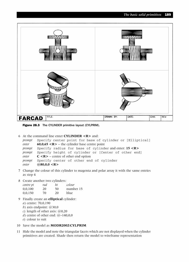
6 At the command line enter CYLINDER <R> and:prompt Specify center point for base of cylinder or [Elliptical]enter 60,0,65 <R> – the cylinder base centre pointprompt Specify radius for base of cylinder and enter: 15 <R>prompt Specify height of cylinder or [Center of other end]enter C <R> – centre of other end optionprompt Specify center of other end of cylinderenter @80,0,0 <R>
7 Change the colour of this cylinder to magenta and polar array it with the same entriesas step 4
8 Create another two cylinders:centre pt rad ht colour0,0,100 20 50 number 150,0,150 70 20 blue
9 Finally create an elliptical cylinder:a) centre: 70,0,190b) axis endpoint: @30,0c) length of other axis: @0,20d) centre of other end: @–140,0,0e) colour to suit
10 Save the model as MODR2002\CYLPRIM
11 Hide the model and note the triangular facets which are not displayed when the cylinderprimitives are created. Shade then return the model to wireframe representation
The basic solid primitives 189
Figure 28.3 The CYLINDER primitive layout (CYLPRIM).
modelling with AutoCAD.qxd 17/06/2002 15:40 Page 189

12 Investigatea) With the 3D viewport active, enter ISOLINES at the command line and enter a value
of 6. Enter REGEN <R> and note model displayb) change the ISOLINES value to 48 and regenc) return the ISOLINES value to the original 12d) enter FACETRES at the command line and alter the value to 2, then enter HIDE <R>.
Note the effect, then regene) alter FACETRES to 5, hide, then regenf) return FACETRES to 1
13 NoteThe ISOLINES system variable controls the appearance of primitive curved surfaces whenthey are created. The triangulation effect, or FACETS, is controlled by the system variableFACETRES. The higher the value of FACETRES (max 10) then the ‘better the appearance’of curved surfaces, but the longer it takes for hide and shade. At our level, the values of12 for ISOLINES and 1 for FACETRES are sufficient.
The CONE primitive – Fig. 28.41 Open the A3SOL template file, MVLAY1, UCS BASE etc
2 Menu bar with Draw-Solids-Cone and:prompt Specify center point for base of cone or [Elliptical]enter 0,0,0 <R> – the cone base centre pointprompt Specify radius for base of cone or [Diameter]enter 50<R>prompt Specify height of cone or [Apex]enter 60 <R>
3 Create another cone with:a) centre: 0,0,0b) radius: 90c) height: –80d) colour: green
4 Centre each viewport about the point 0,0,10 at 200 mag
5 Select the CONE icon from the Solids toolbar and:prompt Specify center point for base of cone or [Elliptical]enter E <R> – the elliptical optionprompt Specify axis endpoint of ellipse for base of cone or
[Center]enter C <R> – the centre point optionprompt Specify center point of ellipse for base of coneenter 70,0,0 <R>prompt Specify axis endpoint of ellipse for base of cone and enter:
@20,0,0 <R>prompt Specify length of other axis for base of cone and enter:
@0,25,0 <R>prompt Specify height of cone or [Apex] and enter: 35 <R>
6 Change the colour of this cone to blue, then polar array it with:a) centre point: 0,0b) items: 5c) full angle to fill, with rotation
190 Modelling with AutoCAD 2002
modelling with AutoCAD.qxd 17/06/2002 15:40 Page 190
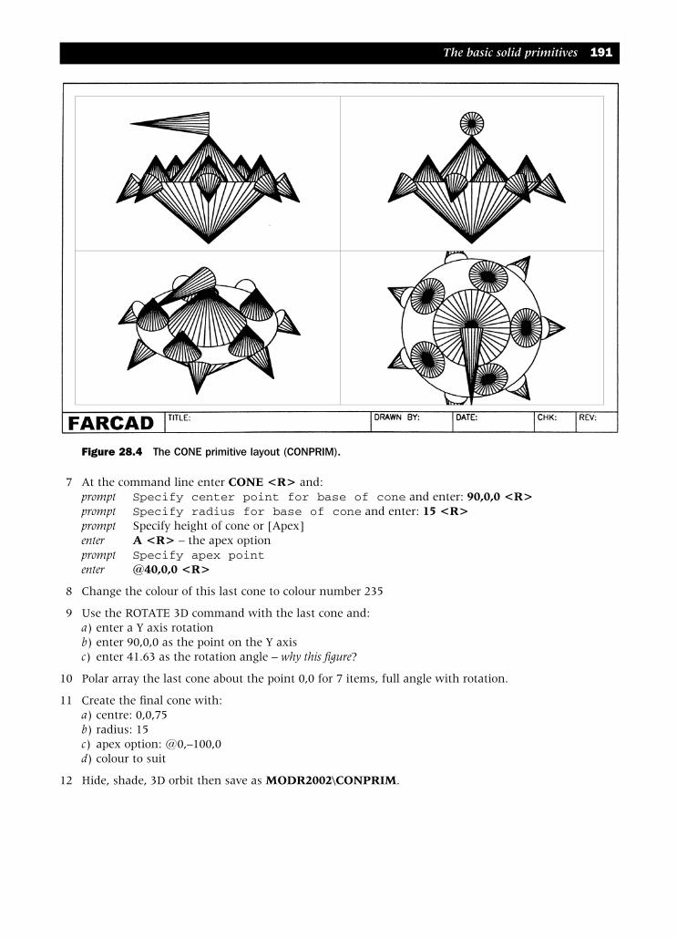
7 At the command line enter CONE <R> and:prompt Specify center point for base of cone and enter: 90,0,0 <R>prompt Specify radius for base of cone and enter: 15 <R>prompt Specify height of cone or [Apex]enter A <R> – the apex optionprompt Specify apex pointenter @40,0,0 <R>
8 Change the colour of this last cone to colour number 235
9 Use the ROTATE 3D command with the last cone and:a) enter a Y axis rotationb) enter 90,0,0 as the point on the Y axisc) enter 41.63 as the rotation angle – why this figure?
10 Polar array the last cone about the point 0,0 for 7 items, full angle with rotation.
11 Create the final cone with:a) centre: 0,0,75b) radius: 15c) apex option: @0,–100,0d) colour to suit
12 Hide, shade, 3D orbit then save as MODR2002\CONPRIM.
The basic solid primitives 191
Figure 28.4 The CONE primitive layout (CONPRIM).
modelling with AutoCAD.qxd 17/06/2002 15:40 Page 191

The SPHERE primitive – Fig. 28.51 Open the A3SOL template file, UCS BASE etc
2 Menu bar with Draw-Solids-Sphere and:prompt Specify center of sphere<0,0,0>enter 0,0,0 <R>prompt Specify radius of sphere or [Diameter]enter 60 <R>
3 Centre each viewport about 0,0,20 at 200 magnification
4 Select the SPHERE icon from the Solids toolbar and:prompt Specify center of sphere<0,0,0>enter 80,0,0 <R>prompt Specify radius of sphere or [Diameter]enter D <R> – the diameter optionprompt Specify diameter and enter: 40 <R>
5 Change the colour of this sphere to green, then polar array it:a) about the point: 0,0b) for 5 itemsc) full angle with rotation
6 At the command line enter SPHERE <R> and create a sphere with:a) centre: 0,0,75b) radius: 15c) colour: magenta
192 Modelling with AutoCAD 2002
Figure 28.5 The SPHERE primitive layout (SPHPRIM).
modelling with AutoCAD.qxd 17/06/2002 15:40 Page 192

7 Restore UCS FRONT and polar array the magenta sphere about the point 0,0 for 3 itemswith full angle rotation
8 Restore UCS BASE and create the final sphere with:a) centre: 58,0,70b) radius: 30c) colour blued) polar array about 0,0 for 3 items, full angle rotation
9 Hide, shade, save as MODR2002\SPHPRIM
10 Investigatea) ISOLINES set to 48 then regenb) ISOLINES set to 5 then regenc) Restore original ISOLINES 18d) FACETRES set to 10 then hide and regene) Note the appearance of the sphere primitives with these system variable values.
The TORUS primitive – Fig. 28.61 A3SOL template file with UCS BASE, MVLAY1 layout etc
2 Menu bar with Draw-Solids-Torus and:prompt Specify center of torus<0,0,0>enter 0,0,0 <R>prompt Specify radius of torus or [Diameter]enter 80 <R>prompt Specify radius of tube or [Diameter]enter 15 <R>
3 Zoom extents then zoom to a scale of 1 in each viewport
4 Restore UCS FRONT and select the TORUS icon from the Solids toolbar and:prompt Specify center of torus<0,0,0>enter 80,0,0 <R>prompt Specify radius of torus and enter: 50 <R>prompt Specify radius of tube and enter: 20 <R>
5 Change the colour of this torus to blue
6 Restore UCS BASE and polar array the blue torus about 0,0 for 3 items with full circlerotation
7 Restore UCS RIGHT, enter TORUS <R> at the command line and create a torus with:a) centre: 0,0,–95b) radius of torus: 80c) radius of tube: 20d) colour: green
8 Restore UCS BASE and create the final torus with:a) centre: 80,0,80b) radius of torus: 50c) radius of tube: 20d) colour: to suit
9 Save as MODR2002\TORPRIM
The basic solid primitives 193
modelling with AutoCAD.qxd 17/06/2002 15:40 Page 193
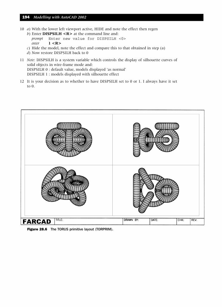
10 a) With the lower left viewport active, HIDE and note the effect then regenb) Enter DISPSILH <R> at the command line and:
prompt Enter new value for DISPSILH <0>enter 1 <R>
c) Hide the model, note the effect and compare this to that obtained in step (a)d) Now restore DISPSILH back to 0
11 Note: DISPSILH is a system variable which controls the display of silhouette curves ofsolid objects in wire-frame mode and:DISPSILH 0 : default value, models displayed ‘as normal’DISPSILH 1 : models displayed with silhouette effect
12 It is your decision as to whether to have DISPSILH set to 0 or 1. I always have it set to 0.
194 Modelling with AutoCAD 2002
Figure 28.6 The TORUS primitive layout (TORPRIM).
modelling with AutoCAD.qxd 17/06/2002 15:40 Page 194

Summary1 The six solid primitives can be activated:
a) from the menu bar with Draw-Solidsb) by icon selection from the Solids toolbarc) by entering the solid name at the command line
2 The corner/centre start points can be:a) entered as coordinates from the keyboardb) referenced to existing objectsc) picking suitable points on the screen
3 The six primitives have various options:box: a) corner; centre
b) cube; length, width, height; other cornerwedge: a) corner; centre
b) cube; length, width, height; other cornercylinder: a) circular; elliptical
b) radius; diameterc) height; centre of other end
cone: a) circular; ellipticalb) radius; diameterc) height; apex point
sphere: a) centre onlyb) diameter; radius
torus: a) centre onlyb) radius of torus; diameterc) radius of tube; diameter
AssignmentA single activity for your imaginative mind.
Activity 18: A solid primitive layout.
Create a layout of your own design with the six basic primitives using the followinginformation and with your own colours:
Box Wedge Cylinder Conelength: 100 length: 50 radius: 20 radius: 50width: 40 width: 60 height: 80 height: 120height: 30 height: 50
Sphere Torusradius: 40 torus rad: 50
tube rad: 20
The basic solid primitives 195
modelling with AutoCAD.qxd 17/06/2002 15:40 Page 195

The swept solidprimitivesSolid models can be generated by extruding or revolving ‘shapes’ and in this chapter wewill use several exercises to demonstrate how complex solids can be created fromrelatively simple shapes.
Extruded solidsSolid models can be created by extruding CLOSED OBJECTS such as polyline shapes,polygons, circles, ellipses, splines and regions:a) to a specified height and taper angleb) along a path.
Extruded example 1: letters1 Open your A3SOL template file, layer MODEL, MVLAY1 and display the Solids toolbar
2 Change the viewpoint in lower left viewport with the command line entry VPOINT <R>and:prompt Specify a view point or [Rotate]enter R <R> – the rotate optionthen enter angles of 30 and 30
3 Make the upper left viewport active and restore UCS RIGHT
4 Using the reference sizes given in Fig. 29.1:a) draw the three letters M, T and C as closed shapes using line and arc segmentsb) use Modify-Object-Polyline from the menu bar to ‘convert’ the three outlines into
a single polyline with the Join optionc) use your discretion for sizes not given (a snap of 5 helps)d) use the start points A, B and C given
5 Still with UCS RIGHT, zoom centre about 0,50,0 at 200 in the 3D viewport and 300 inthe other three viewports
6 Menu bar with Draw-Solids-Extrude and:prompt Select objectsrespond pick the letter M then right-clickprompt Specify height of extrusion or [Path]enter 80 <R>prompt Specify angle of taper for extrusion enter 0 <R>
7 The letter M will be extruded for a height of 80 in the positive Z direction.
Chapter 29
modelling with AutoCAD.qxd 17/06/2002 15:40 Page 196

8 Select the EXTRUDE icon from the Solids toolbar and:prompt Select objectsrespond pick the letter T then right-clickprompt Specify height of extrusion or [Path]enter 50 <R>prompt Specify angle of taper for extrusionenter 5 <R>
9 At the command line enter EXTRUDE <R> and:a) objects: pick the letter C then right-clickb) height: enter –50c) taper angle: enter –3
10 Hide and shade etc, then save the model with your own name
The swept solid primitives 197
Figure 29.1 Extruded example 1 – letters.
modelling with AutoCAD.qxd 17/06/2002 15:40 Page 197

Extruded example 2: keyed splined shaft1 Open the A3SOL template file, layer MODEL, MVLAY1, UCS BASE and the lower right
viewport active.Note: in future exercises when I refer to opening A3SOL these are the ‘normal settings’I expect, i.e. layer MODEL current, MVLAY1 tab active, UCS BASE current and the lowerleft (3D) viewport active. I will thus only say: Open A3SOL file.
2 Zoom centre about 0,0,–20 at 150 magnification in all viewports
3 Refer to Fig. 29.2 and create two profiles:a) an outer tooth profile from two circles and an arrayed line, then trim as required. The
circle centres should be at 0,0b) an inner shaft profile to your own specification
4 Use the menu bar sequence Modify-Object-Polyline (or PEDIT at the command line) toconvert each profile into a single polyline using the Join option.
5 Alter the system variables ISOLINES to 6 and FACETRES to 0.5
6 Select the EXTRUDE icon from the Solids toolbar and:prompt Select objectsrespond pick the outer tooth profile then right-clickprompt Specify height of extrusion or [Path]enter –70 <R>prompt Specify angle of taper for extrusionenter –3 <R>
7 Repeat the Extrude icon selection and:a) objects: pick the inner shaft profile then right-clickb) height: enter 30c) taper: enter 0d) note the ‘denseness’ of the model sides
8 Gouraud shade the model and use 3D orbit in the 3D viewport
9 Restore the original display with the menu bar sequence View-Shade-2D Wireframe
10 Save the model layout
198 Modelling with AutoCAD 2002
Figure 29.2 Extruded example 2 – splined shaft.
modelling with AutoCAD.qxd 17/06/2002 15:41 Page 198

Extruded example 3: a moulding1 Open the A3SOL template file with ‘normal settings’
2 Centre the viewports about the point 120,75,35 at 300 mag
3 Draw a polyline with:start point: 0,0next point: @0,100arc option with endpoint: @100,0arc endpoint: @100,–100line option with endpoint: @100,0 then right-click/enter
4 Change the colour of the polyline to blue
5 Restore UCS FRONT and make the top right viewport active
6 Use the reference sizes in Fig. 29.3 to create the moulding as a single polyline or createyour own outline design if required.
7 Make the lower left viewport active
8 Set ISOLINES to 12
9 Select the EXTRUDE icon from the Solids toolbar and:prompt Select objectsrespond pick the red polyline then right-clickprompt Specify height of extrusion or [Path]enter P <R> – the path optionprompt Select extrusion pathrespond pick the blue polylineand the red outline is extruded along the blue path
10 Shade the model, 3D orbit then restore to original wireframe model
11 Save the model layout
The swept solid primitives 199
Figure 29.3 Extruded example 3 – a moulding.
modelling with AutoCAD.qxd 17/06/2002 15:41 Page 199

Extruded example 4: a polygon type duct arrangement1 Open the A3SOL template file with normal settings
2 Create a 5 segment 3D polyline with the menu bar sequence Draw-3D Polyline and:prompt Specify start point of polyline and enter: 0,0 <R>prompt Specify endpoint of line and enter: @0,0,100 <R>prompt Specify endpoint of line and enter: @100,0,100 <R>prompt Specify endpoint of line and enter: @100,100,0 <R>prompt Specify endpoint of line and enter: @0,100,100 <R>prompt Specify endpoint of line and enter: @100,100,–100 <R>prompt Specify endpoint of line and: right-click/enter
3 Change the colour of the 3D polyline to green
4 In each viewport, zoom centre about 150,150,175 at 400 mag.
5 Draw a polygon with:a) sides: 6b) centre: 0,0c) inscribed in a circle of radius 40
6 Select the EXTRUDE icon and:a) objects: pick the red polygon then right-clickb) enter P <R> for the path optionc) path: pick the green 3D polyline
7 The polygon will be extruded along the green path to give a ducting effect.
8 Shade, 3D orbit then save
9 Question: Green polyline but red model – why?
This completes the extrusion exercises.
200 Modelling with AutoCAD 2002
Figure 29.4 Extruded example 4 – a polygon duct effect.
modelling with AutoCAD.qxd 17/06/2002 15:41 Page 200

Revolved solidsSolid models can be created by revolving objects (closed polylines, polygons, circles,ellipses, closed splines, regions):a) about the X and Y axesb) about selected objects by a specified angle.
As with extrusions, very complex models can be obtained from relatively simple shapes.
Revolved example 1: a flagon1 Open the A3SOL template file as normal and in each viewport zoom centre about
0,80,0 at 200 mag.
2 a) Set ISOLINES to 8b) In the top left viewport, alter the viewpoint with VPOINT at the command line, select
the ROTATE option and enter angles of 30 and –20
3 Restore UCS FRONT and make the top right viewport active
4 Refer to Fig. 29.5 and draw a closed polyline outline using the sizes given as a reference– or design your own
5 Menu bar with Draw-Solids-Revolve and:prompt Select objectsrespond pick the polyline then right-clickprompt Specify start point for axis of revolution or define axis
by [Object/X (axis)/Y (axis)]enter Y <R> – the Y axis optionprompt Specify angle of revolutionrespond right-click to accept the 360 (full circle) default
6 The polyline outline will be revolved into a swept revolved solid
7 Shade one of the 3D viewports and use 3D orbit
8 Save the completed model
The swept solid primitives 201
Figure 29.5 Revolved example 1 – a flagon.
modelling with AutoCAD.qxd 17/06/2002 15:41 Page 201

Revolved example 2: a shaft1 Open the A3SOL template file with normal settings
2 Make the lower right viewport active
3 In each viewport zoom centre about 50,0,0 at 200 magnification
4 Refer to Fig. 29.6 and draw a closed polyline outline using the sizes given. Use the(0,–30) start point. Note that I have only displayed the 3D viewport with this exercise.This was for convenience purposes only
5 Set ISOLINES to 12
6 Menu bar with Draw-Solids-Revolve and:prompt Select objectsrespond pick the polyline then right-clickprompt Specify start point of axis of revolution or define axis
by [Object/X (axis)/Y (axis)]enter X <R> – the X axis optionprompt Specify angle of revolutionenter 360 <R>
7 The polyline outline will be revolved about the X axis as fig(a)
8 Observe the effect then undo the revolved effect to restore the original polyline outline
202 Modelling with AutoCAD 2002
Figure 29.6 Revolved example 2 – a shaft.
modelling with AutoCAD.qxd 17/06/2002 15:41 Page 202

9 Select the revolve icon from the solids toolbar and: a) objects: select the polyline outline then right-clickb) axis of revolution: X axisc) angle of revolution: 250d) the revolved effect will be as fig(b). Observe then undo
10 At the command line enter REVOLVE <R> and:a) objects: select polyline then right-clickb) axis of revolution: enter Y <R>c) angle of revolution: 360d) the result will be as fig(c) – pan needed?e) observe then undo the revolved effect
11 Finally revolve the polyline:a) about the Y axisb) with a 300 angle of revolution – fig(d)
10 Shade, 3D orbit, etc. then save if required
This completes the swept primitive exercises.
Plotting multiple viewport layouts with hideTo obtain a plot of a multiple layout with hide, the user needs the use the MVIEWcommand. To demonstrate this command:
1 Open any multiple viewport drawing, e.g. the splined shaft example
2 Enter paper space
3 At the command line enter MVIEW <R> and:prompt Specify corner of viewport or [various options]enter H <R> – the hideplot optionprompt Hidden line removal for plotting [ON/OFF]enter ON <R>prompt Select objectsrespond pick the borders of all viewports which have to have hidden line
removalthen right-click
4 The command line is returned
5 Proceed with the normal plot sequence, but ensure that the Hide Plot option is NOTACTIVE (i.e. no tick)
6 This procedure should be used at all times when multi-viewport plots are required withhidden line removal
The swept solid primitives 203
modelling with AutoCAD.qxd 17/06/2002 15:41 Page 203

Summary1 Swept solids are obtained with the extrude and revolve commands
2 The two commands can be activated:a) by icon selection from the Solids toolbarb) from the command line with Draw-Solidsc) by entering EXTRUDE and REVOLVE at the command line
3 Very complex models can be obtained from simple shapes
4 Only certain ‘shapes’ can be extruded/revolved. These are closed polylines, circles, ellipses,polygons, closed splines and regions (more on this in a later chapter)
5 Objects can be extruded:a) to a specified heightb) with/without a taper anglec) along a path curve
6 The extruded height is in the Z direction and can be positive or negative
7 The taper angle can be positive or negative
8 Objects can be revolved:a) about the X and Y axesb) about an objectc) by specifying two points on the axis of revolution
9 The angle of revolution can be full (360) or partial.
AssignmentDuring the excavation of the ancient city of CADOPOLIS, the intrepid diggers uncoveredtwo artefacts, both of which they attributed to our master builder MACFARAMUS. Theydecided (how we will never know), that the artefacts were scale models of a pyramidand the partial wheel from a chariot. It is these that you have to create as solid modelsfrom swept primitives.
Activity 19: Two swept primitive models designed by MACFARAMUS.
These two models have to be created from closed polylines. The dimensions taken bythe site engineers were not complete and only the basic sizes have been given. You haveto use your own discretion when drawing the two outlines. The procedure for bothmodels is:
1 Open your template file as normal
2 Draw the outline of the model as a closed polyline, both with UCS BASE, layer MODELand with the lower right viewport active
3 Extrude the pyramid outline for a height of 150 and a taper angle of 10
4 Revolve the wheel outline about the X or Y axis dependent on how the original outlinewas drawn. The partial angle of revolution is to be 270 degrees
5 Centre the models in the viewports
6 Note: I have displayed both models on the one sheet of paper with:a) pyramid: 3D and front viewsb) wheel: two 3D views, from above and from below
204 Modelling with AutoCAD 2002
modelling with AutoCAD.qxd 17/06/2002 15:41 Page 204

Boolean operationsand composite solidsThe basic and swept solids which have been created are called primitives and are the‘basic tools’ for solid modelling. With these primitives the user can create compositesolids, so called because they are ‘composed’ of two or more solid primitives, i.e.a) primitive: a box, wedge, cylinder, extrusion, etc.b) composite: a solid made from two or more primitives.
Composite solids are created from primitives using the three Boolean operations ofunion, subtraction and intersection. Figure 30.1 demonstrates these operations with twoprimitives: a) a boxb) a cylinder ‘penetrating’ the box
Chapter 30
Figure 30.1 The three BOOLEAN operations.
modelling with AutoCAD.qxd 17/06/2002 15:41 Page 205

Union1 This operation involves ‘joining’ two or more primitives to form a single composite, the
user selecting all objects to be unioned
2 The operation can be considered similar to welding two or more components together.
Subtraction1 This involves removing one or more solids from another solid thereby creating the
composite. The user selects:a) the source solidb) the solids to be subtracted from the source solid
2 The result of a subtraction operation can be likened to a drilled hole, i.e. if the cylinderis subtracted from the box, a hole will obtained in the box.
3 Note: the source solid is generally ‘the larger solid’ i.e. you cannot normally take a largesolid from a small solid
Intersection1 This operation gives a composite solid from other solids which have a common volume,
the user selecting all objects which have to be intersected
2 The box/cylinder illustration of the intersection operation gives a ‘disc shape’ or ‘hole’i.e. if the box and cylinder are intersected, the common volume is the disc shape.
Creating a composite solid from primitivesThere is no ‘correct or ideal’ method of creating a composite, i.e. the Boolean operationsselected by one user may be different from those selected by another user, but the finalcomposite may be the same. To demonstrate this, we will create an L-shaped componentby three different methods, so:
1 Open your A3SOL template file refer to Fig. 30.2 and:a) enter paper spaceb) erase any text and the four viewportsc) with layer VP current create a single viewport with:
i) first point: pick to suit in lower left corner areaii) other corner: enter @360,220
d) return to model space, UCS BASE, layer MODELe) set a SE Isometric viewpoint
2 Create two box primitives:a) corner: 0,0,0 b) corner: 100,100,100
cube option length: –60length: 100 width: –100colour: red height: –70
colour: blue
3 Create another two box primitives:a) corner: 125,125,0 b) corner: 125,125,30
length: 100 length: 40width: 100 width: 100height: 30 height: 70colour: red colour: blue
206 Modelling with AutoCAD 2002
modelling with AutoCAD.qxd 17/06/2002 15:41 Page 206

4 Restore UCS FRONT and draw a 2D polyline shape:start pt: 500,250 next pt: @100,0 next pt: @0,30next pt: @–60,0 next pt: @0,70 next pt: @–40,0next pt: close
5 Restore UCS BASE and zoom centre about 100,250,0 at 400 mag.
6 From the menu bar select Modify-Solids Editing-Subtract and:prompt Select solids and regions to subtract from..
Select objectsrespond pick the left red box then right-clickprompt Select solids and regions to subtract..
Select objectsrespond pick the left blue box then right-clickand the blue box is subtracted from the red box
7 Menu bar with Modify-Solids Editing-Union and:prompt Select objectsrespond pick the middle red and blue boxes then right-clickand the two boxes will be unioned
8 Restore UCS FRONT and:a) select the EXTRUDE icon from the Solids toolbarb) pick the L shaped polyline then right-clickc) enter an extruded height of –100 with 0 taperd) the L-shape polyline is extruded into a composite
Boolean operations and composite solids 207
Figure 30.2 Creating the same composite by three different methods.
modelling with AutoCAD.qxd 17/06/2002 15:41 Page 207

9 Taska) Hide the models – all the sameb) Gouraud shade the models and note colour effect between the union and subtraction
composites – any comment?c) Return to 2D wireframe representationd) Menu bar with Tools-Inquiry-Region/Mass Properties and:
prompt Select objectsrespond pick left composite then right-clickand AutoCAD Text Window with:
Mass: 580000.00Volume: 580000.00Bounding box, Centroid etc.
enter N <R> in response to ‘Write analysis to file’ promptd) Repeat the MASSPROP command and select the middle and right composites – same
mass and volume?
10 Questionsa) Why are the mass and volume the same?
Answer: AutoCAD 2002 assumes a density value of 1 and does not support differentmaterial densities
b) Is the volume of 580000 correct for the L shape?c) What are the volume units?
11 Now that we have investigated the Boolean operations, we will create some compositesolid models which (I hole) will be interesting.
Summary1 There are three Boolean operations – union, subtraction and intersection
2 The three operations can be activated:a) from the menu bar with Modify-Solids Editingb) in icon form from the Solids Editing toolbarc) by entering the command from the keyboard.
3 The Boolean operations are derived from Boolean Algebra (set theory) and are essentialfor the creation of solid composites from primitives.
208 Modelling with AutoCAD 2002
modelling with AutoCAD.qxd 17/06/2002 15:41 Page 208
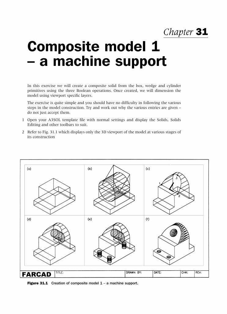
Composite model 1 – a machine supportIn this exercise we will create a composite solid from the box, wedge and cylinderprimitives using the three Boolean operations. Once created, we will dimension themodel using viewport specific layers.
The exercise is quite simple and you should have no difficulty in following the varioussteps in the model construction. Try and work out why the various entries are given –do not just accept them.
1 Open your A3SOL template file with normal settings and display the Solids, SolidsEditing and other toolbars to suit.
2 Refer to Fig. 31.1 which displays only the 3D viewport of the model at various stages ofits construction
Chapter 31
Figure 31.1 Creation of composite model 1 – a machine support.
modelling with AutoCAD.qxd 17/06/2002 15:41 Page 209

3 In each viewport, zoom-extents then zoom to 1.5 scale
4 With the 3D viewport active, use the BOX icon to create two primitives as fig(a) with:a) corner: 0,0,0 b) corner: 100,120,25
length: 100 length: –100width: 150 width: –90height: 25 height: 60colour: red colour: blue
5 Create a cylinder on top of the blue box with:a) centre: 50,30,85b) radius: 50c) height/other end: enter C <R> then @0,90,0 <R>d) colour: green
6 Create a wedge with:a) corner: 0,120,85b) length: 70; width: 100; height: 70c) colour: magenta
7 Rotate (2D rotate) the magenta wedge:a) about the point: 0,120,85b) by: –90 degrees to give fig(b)
8 Select the INTERSECTION icon from the Solids Editing toolbar and:prompt Select objectsrespond pick the green cylinder and magenta wedge then right-click
9 Select the UNION icon from the Solids Editing toolbar and: prompt Select objectsrespond pick the red and blue boxes and the intersected wedge/cylinder then
right-click
10 The model now appears as fig(c)
11 Refer to fig(c) and menu bar with Tools-New UCS-3 Point and set a new UCS with:a) origin: MIDpoint icon and pick line 12b) X axis: ENDpoint icon and pick pt2c) Y axis: QUADrant icon and pick pt3 on curve
12 The UCS icon will move and align itself on the sloped surfaceNote: if icon does not move, menu bar with View-Display-UCS Icon and ensure that Onand Origin are ticked
13 Save this UCS position as SLOPE
14 Create a cylinder with:a) centre: 0,35,0b) radius: 18c) height: –100d) colour: number 54 – use the CHPROP command
15 Select the SUBTRACT icon from the Solids Editing toolbar and:prompt Select solids and regions to subtract from..
Select objectsrespond pick the composite model then right-clickprompt Select solids or regions to subtract
Select objectsrespond pick the cylinder then right-click – fig(d)
210 Modelling with AutoCAD 2002
modelling with AutoCAD.qxd 17/06/2002 15:41 Page 210

16 Restore UCS BASE
17 Create a cylinder with:a) centre: 20,15,0b) radius: 9c) height: 25d) colour: number 174
18 Multiple copy the cylinder:a) from: 20,15b) by: @60,0 and by: @30,120
20 Using the SUBTRACT icon:a) select the original composite then right-clickb) pick the three cylinders then right-click
21 The model is now complete and is displayed in fig(e) without hide and in fig(f) withhide.
22 Select the Model tab and Gouraud shade the model, then use the 3D orbit command torotate the shaded model
23 Restore the model to 2D wireframe representation, then make the MVLAY1 tab active
24 At this stage save the composite as MODR2002\MACHSUPP
Making the viewport specific layersThe MVLAY1 tab screen displays the model in a four viewport configuration and we nowwant to add some dimensions. These dimensions must be added on viewport specificlayers and these layers must now be created.
1 At the command line enter VPLAYER <R> and:prompt Enter an option [?/Freeze/Thaw/Reset/Newfrz/Vpvisdflt]enter N <R> – the Newfrz (new viewport freeze) optionprompt Enter name(s) of new layers frozen in all viewportsenter DIMTL,DIMTR,DIMBR <R>prompt Enter an option [?/Freeze/Thaw/..respond right-click – as finished with command
2 The command line entry VPLAYER is to activate viewport layer
3 Make the top left viewport active and menu bar with Format-Layer and:prompt Layer Properties Manager dialogue boxnote three new layers – DIMBR, DIMTL, DIMTR with:
i) Frozen in current viewport – blue iconii) Frozen in new viewport – blue icon
respond 1. activate Show Details 2. pick DIMTL (highlights) and note details – Freeze in current viewport is
on (tick)3. pick blue icon Freeze in active viewport to Thaw the layer and the tick
is removed from Freeze in current viewport details list4. pick OK
4 With the top right viewport active, Format-Layer and:a) pick layer DIMTRb) toggle the blue Freeze in current viewport icon to yellow to
Thaw layer DIMTR in the top right viewportc) pick OK
Composite model 1 – a machine support 211
modelling with AutoCAD.qxd 17/06/2002 15:41 Page 211

5 With lower right viewport active, Format-Layer and:a) pick layer DIMBRb) toggle Freeze icon in current viewport from blue to yellow, i.e. from Frozen to Thaw
to Thaw layer DIMBR in the lower right viewportc) pick OK
6 What has been achieved in this section?a) three new viewport specific layers have been madeb) these layers have been named DIMTL for the top left viewport, DIMTR for the top
right viewport and DIMBR for the bottom left viewportc) the three layers were originally created :
i) frozen in new viewportsii) currently frozen in all viewports
d) each layer was currently thawed in a specific viewport, e.g. layer DIMTL is currentlythawed in the top left viewport but is currently frozen in the other three viewports.Layers DIMTR and DIMBR are currently frozen in the top left viewport.
7 Before adding the dimensions, change the colour of the three new layers (DIMTL,DIMTR, DIMBR) to magenta using the Layer Properties Manger dialogue box.
Adding the dimensions1 Before the dimensions are added to the model, menu bar with Dimension-Style and
using the Dimension Style Manager dialogue box:a) 3DSTD the current (and only) style?b) pick Modifyc) pick the Fit tabd) Alter Scale for Features: Use overall scale of 2e) pick OK to return to Dimension Style Manager dialogue boxf) pick Close
2 This will scale all the dimension parameters by 2
3 Make the lower right viewport active and:a) restore UCS BASEb) make layer DIMBR currentc) refer to Fig. 31.2
4 With Dimension-Linear from the menu bar, or with the LINEAR dimension icon fromthe Dimensions toolbar, add:a) the horizontal dimensionb) the four vertical dimensions using the baseline option
5 With the top right viewport active:a) restore UCS FRONTb) make layer DIMTR currentc) add the two linear dimensions
6 Make the top left viewport active and:a) restore UCS RIGHTb) make layer DIMTL currentc) add the six dimensions
7 The composite model is now complete with dimensions added and can be plotted withthe layer VP frozen for effect – Fig. 31.2
8 These dimension additions do not need to be saved.
212 Modelling with AutoCAD 2002
modelling with AutoCAD.qxd 17/06/2002 15:41 Page 212
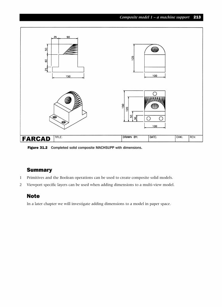
Summary1 Primitives and the Boolean operations can be used to create composite solid models.
2 Viewport specific layers can be used when adding dimensions to a multi-view model.
NoteIn a later chapter we will investigate adding dimensions to a model in paper space.
Composite model 1 – a machine support 213
Figure 31.2 Completed solid composite MACHSUPP with dimensions.
modelling with AutoCAD.qxd 17/06/2002 15:41 Page 213

Composite model 2 – a backing plateIn this exercise we will create a solid from an extruded swept primitive an then subtractvarious ‘holes’ to complete the composite. The exercise will also involve altering theviewport layout of the A3SOL template file which is an interesting exercise in itself. Aswith all the exercises, do not just accept the entries – work out why the various valuesare being used.
The modelRefer to Fig. 32.1 which details the model to be created and gives the relevant sizes. Asan aside draw the three orthogonal views as given and then add the isometric (the arc‘hole’ is interesting to complete in an isometric view). Time how long it takes to completethis 2D drawing. I spent about an hour to complete the four views with dimensions.
Chapter 32
Figure 32.1 Backing plate drawn as orthogonal views and as isometric.
modelling with AutoCAD.qxd 17/06/2002 15:41 Page 214

Setting the viewports1 Open your A3SOL template file and with MVLAY1 tab active:
a) enter paper spaceb) erase the four viewportsc) make layer VP currentd) refer to Fig. 32.2
2 Menu bar with View-Viewports–1 Viewport and:prompt Specify first corner and enter: 10,25 <R>prompt Specify other corner and enter: @155,175 <R>
3 Create another three single viewports using the following coordinate entries:a) first corner: 165,25
other corner: @160,70b) first corner: 165,95
other corner: @160,155c) first corner: 325,95
other corner: @70,155
4 In model space:a) make layer MODEL currentb) set UCSVP to 0 in each viewportc) set the 3D viewpoints in the viewports as fig(a)d) restore UCS BASEe) zoom centre about 0,10,60 at 1XP – yes enter 1XPf) in paper space zoom in on viewport B then model space with viewport B active
Composite model 2 – a backing plate 215
Figure 32.2 Steps in the creation of the backing plate composite.
modelling with AutoCAD.qxd 17/06/2002 15:41 Page 215

Creating the extrusion1 Using the polyline icon from the Draw toolbar, create a single polyline from line and arc
segments with the following entries:Start point 0,0Next point @27,0Next point Arc option, with endpoint of arc @2,2Next point Line option, to @0,22Next point @23,0Next point Arc option, with endpoint of arc @0,–6Next point Line option, to @–17,0Next point @0,–20Next point Arc option, with endpoint of arc @–4,–4Next point Line option, to @–31,0Next point right-click/enter
2 Mirror the polyline shape about the points 0,0 and 0,50 and do not delete source objects
3 Use the menu bar sequence Modify-Object-Polyline and:a) pick any point on the right-hand polylineb) enter J <R> – the join optionc) pick the two polyline shapes then right-clickd) enter X <R> to end the command
4 The two ‘halves’ of the polyline have been joined into a single polyline as fig(b) in planview and fig(c) in 3D.
5 At the command line enter ISOLINES <R> and:prompt Enter new value for ISOLINES<24>enter 3 <R>
6 Note: the ISOLINES system variable has been reduced from 18 to 3 due to the ‘corneredges’ of the model. With a value of 18, the extrusion would result in these corner edgesbeing displayed ‘very dense’.
7 Select the EXTRUDE icon from the Solids toolbar and:prompt Select objectsrespond pick any point on the polyline then right-clickprompt Specify height of extrusion or [Path] and enter: 120 <R>prompt Specify angle of taper for extrusion and enter: 0 <R>
8 The polyline shape will be extruded as fig(d)
9 Paper zoom-previous then return to model space
216 Modelling with AutoCAD 2002
modelling with AutoCAD.qxd 17/06/2002 15:41 Page 216

Creating the ‘holes’1 Restore UCS FRONT with viewport C active
2 Create a box primitive with:a) corner: –5,30,0b) length: 10; width: 50; height: 6c) colour: blue
3 Create the following three primitives:box cylinder cylindercorner: –10,85,0 centre: –10,95,0 centre: 10,95,0length: 20 radius: 10 radius: 10width: 20 height: 6 height: 6height: 6 colour: green colour: greencolour: green
4 Union the three green primitives
5 Draw two circles:a) centre: 0,30 with radius: 20b) centre: 0,50 with radius: 30c) both circles colour green
6 Trim the circles ‘to each other’ and fillet the ‘corners’ with a radius of 2
7 Convert the four arcs into a single polyline with the menu bar sequence Modify-Object-Polyline using the Join option
8 Extrude the arced polyline for a height of 6 with 0 taper, then change the colour of theextrusion to green
9 Subtract the green and blue ‘holes’ from the red extrusion to display the model as fig(e)
10 Create the following two primitives:cylinder boxcentre: 45,20,–24 corner: 45,15,–24radius: 5 length: 30height: 6 width: 10colour: magenta height: 6
colour: magenta
11 Union these two magenta primitives
12 Rectangular array the magenta cylinder/box composite:a) for 3 rows and 1 columnb) row distance: 40
13 Mirror the three arrayed magenta composites about the points 0,0 and 0,50 and do notdelete the source objects
14 Subtract the six magenta composites from the red extrusion
15 The model is now complete – fig(f) and the four viewport layout should be displayed asFig. 32.3
16 Save the model layout as MODR2002\BACKPLT
17 Shade and use the 3D orbit command in the 3D viewport, then return the model towireframe representation.
Composite model 2 – a backing plate 217
modelling with AutoCAD.qxd 17/06/2002 15:41 Page 217
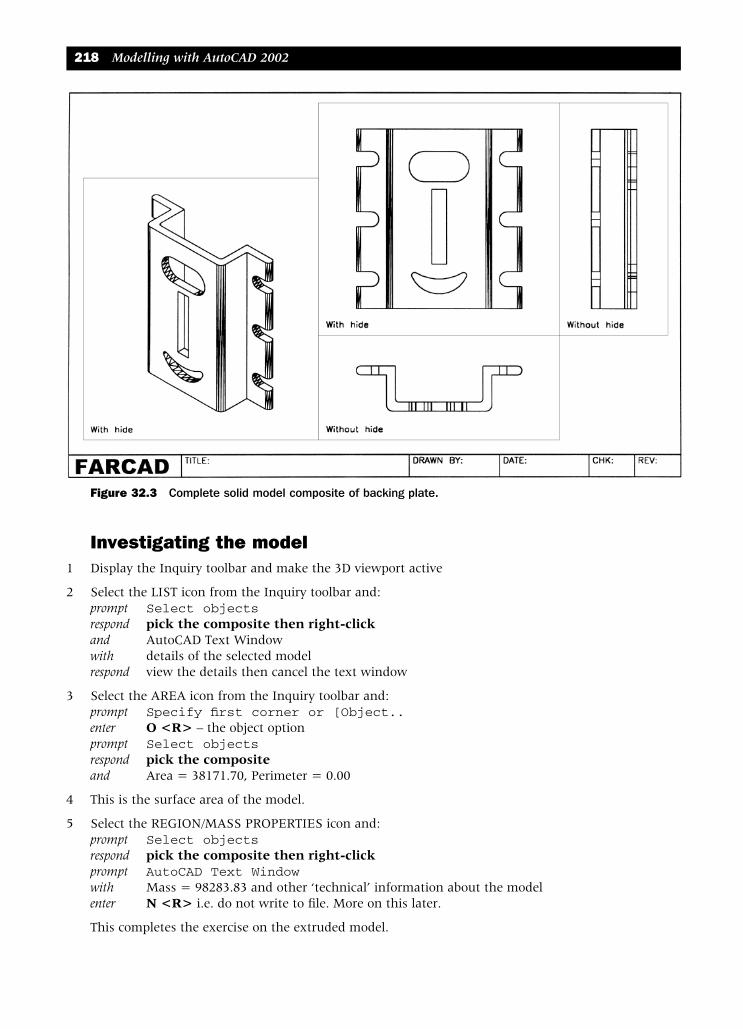
Investigating the model1 Display the Inquiry toolbar and make the 3D viewport active
2 Select the LIST icon from the Inquiry toolbar and:prompt Select objectsrespond pick the composite then right-clickand AutoCAD Text Windowwith details of the selected modelrespond view the details then cancel the text window
3 Select the AREA icon from the Inquiry toolbar and:prompt Specify first corner or [Object..enter O <R> – the object optionprompt Select objectsrespond pick the compositeand Area = 38171.70, Perimeter = 0.00
4 This is the surface area of the model.
5 Select the REGION/MASS PROPERTIES icon and:prompt Select objectsrespond pick the composite then right-clickprompt AutoCAD Text Windowwith Mass = 98283.83 and other ‘technical’ information about the modelenter N <R> i.e. do not write to file. More on this later.
This completes the exercise on the extruded model.
218 Modelling with AutoCAD 2002
Figure 32.3 Complete solid model composite of backing plate.
modelling with AutoCAD.qxd 17/06/2002 15:41 Page 218

Composite model 3 – a flange and pipe This exercise will involve creating a composite mainly as a revolved swept primitive. Cylinderprimitives will be subtracted from the revolved primitive to complete the composite.
1 Open A3SOL template file as normal
2 With the lower left viewport active, restore UCS RIGHT and draw:a) circle: centre at 0,0 with radius: 30b) circle: centre at 0,0 with radius: 40c) line: start point at –200,0 and next point at @0,100
3 Select the REVOLVE icon from the Solids toolbar and:prompt Select objectsrespond pick the smaller circle then right-clickprompt Specify start point for axis of revolution or define axis
[Object..enter O <R> – the object optionprompt Select an objectrespond pick the lower end of the vertical lineprompt Specify angle of revolutionenter 70 <R>
4 Change the colour of the revolved pipe to green
5 Revolve the larger circle using the same entries as step 3 and change the colour of thepipe to blue
6 Erase the line then subtract the green pipe from the blue pipe.
7 You may need a paper space zoom for this operation?
8 Make the lower right viewport active and restore UCS BASE
9 With the POLYLINE icon from the Draw toolbar, draw a continuous closed polyline withthe following entries:Start point: 0,–30Next point: @0,–10Next point: @10,0Next point: Arc option with endpoint: @10,–10Next point: Line option with endpoint: @0,–50Next point: @30,0Next point: @0,70Next point: close option
Chapter 33
modelling with AutoCAD.qxd 17/06/2002 15:41 Page 219

10 Using the REVOLVE icon from the Solids toolbar:a) pick a point on the polyline then right-clickb) enter X <R> as the axis of revolutionc) enter 360 <R> as the angle
11 Change the colour of the revolved solid to magenta
12 With the top left viewport active, restore USC RIGHT
13 Create a cylinder with:a) centre: 0,100,20b) radius: 25c) height: 30d) colour: number 222
14 Polar array this cylinder about the point 0,0 for five items with 360 fill angle
15 a) Subtract the five cylinders from the magenta flangeb) Union the flange and pipe
16 Centre the model with zoom-extents, then zoom to a scale of 1
17 The model is complete and is displayed in Fig. 33.1. It can now be saved asMODR2002\FLPIPE
18 Select the model tab, Gouraud shade then use 3D orbit. The result is impressive?
19 Note: The three composite models MACHSUPP, BACKPLT and FLPIP will be used in laterchapters to demonstrate other commands.
220 Modelling with AutoCAD 2002
Figure 33.1 The completed composite model 3 – pipe/flange.
modelling with AutoCAD.qxd 17/06/2002 15:41 Page 220

The tab layoutsUntil now all models have been created with the MVLAY1 tab active, simply becausethis is the layout I generally use when creating models.
Figure 33.2 is a compilation of the four tab displays on the one sheet. This in itself is aninteresting exercise, i.e. can you set the viewport configuration as Fig. 33.2 to displaythe FLPIP model as shown. In Fig. 33.2 I centred the model with the zoom-extent, zoom1 effect as used previously.
This completes the revolved composite exercise.
Composite model 3 – a flange and pipe 221
Figure 33.2 The four tab displays of the composite pipe/flange.
modelling with AutoCAD.qxd 17/06/2002 15:41 Page 221

The edge primitivesModels can be modified to include a chamfer and fillet effect. These are the edgeprimitives – the third type of primitive which can be created. In this chapter we willinvestigate how solids can be constructed with these edge primitives.
Note:The term ‘edge primitive’ is not now generally used, the models being considered to havebeen modified or edited.
Example 1 – a box solid1 Open the A3SOL template file with normal settings.
2 Refer to Fig. 34.1(a)
3 Use the BOX icon and create a primitive with:a) corner 0,0,0b) cube option with length: 100
4 Zoom centre about 50,50,50 at 225 magnification
5 Select the CHAMFER icon from the Modify toolbar and:prompt Select first line or [Polyline/Distance..respond pick any line on top surfaceprompt Base surface selectionand a) one face of the cube will be highlighted
b) it will be a ‘side’ or the ‘top’prompt Enter surface selection option [Next/OK (current)]respond a) right-click/enter if top face is highlighted
b) enter N<R> if side face is highlighted to highlight the top face then right-click/enter
prompt Specify base surface chamfer distance and enter: 15 <R>prompt Specify other surface chamfer distance and enter: 25 <R>prompt Select an edge or [Loop]respond a) pick any three sides on top surface
b) right-click/enter
6 The top surface will be chamfered at the selected three edges
7 Note: entering L for loop will allow all edges to be chamfered with a single pick
8 Select the FILLET icon from the Modify toolbar and:prompt Select first object or [Polyline/Radius/Trim]respond pick any line on the base surface of the cubeprompt Enter fillet radius and enter: 20 <R>prompt Select edge or [Chain/Radius]respond pick any three edges of the base then right-click
9 The base of the cube will be filleted at the three selected edges and displayed as fig(a).
Chapter 34
modelling with AutoCAD.qxd 17/06/2002 15:41 Page 222

Example 2 – a cylinder solid1 Erase the cube and at the command line enter ISOLINES <R> and check the
value is 12
2 Use the CYLINDER icon to create a cylinder with:a) centre: 0,0,0b) radius: 50c) height: 100
3 Zoom centre about 0,0,50 at 200 magnification
4 In paper space zoom-in on the 3D viewport then return to model space
5 Select the CHAMFER icon and:prompt Select first line or..respond pick the top surface circle edgeprompt Base surface selectionthen Enter surface selection optionrespond <RETURN> as the required surface is highlightedprompt Specify base surface chamfer distance and enter: 15 <R>prompt Specify other surface chamfer distance and enter: 15 <R>prompt Select an edge or..respond pick top circle edge then right-click/enter
6 The top of the cylinder is chamfered with the entered values
The edge primitives 223
Figure 34.1 Modifying solids with the chamfer/fillet commands.
modelling with AutoCAD.qxd 17/06/2002 15:41 Page 223

7 Select the FILLET icon and:prompt Select first object..respond pick bottom circle of cylinderprompt Enter fillet radius and enter: 25 <R>prompt Select an edge..respond right-click as bottom edge already selected
8 The cylinder is filleted at the base
9 In paper space zoom-previous then return to model space
10 The chamfer/fillet effect of the cylinder is displayed as fig(b)
Example 3: A composite edge primitive solid1 Erase the cylinder model and with MVLAY1 tab, UCS BASE, layer MODEL and the lower
left viewport active, create four primitives with:box cylinder box cylindercorner: 0,0,0 centre: 75,60,0 corner: 50,0,40 centre: 150,0,0length: 150 radius: 40 length: 60 radius: 30width: 120 height: 100 width: 120 height: 100height: 100 colour: green height: 40 colour: magentacolour: red colour: blue
2 In all viewports, zoom centre about 75,60,50 at 200 mag in the 3D viewport and 150 magin the other viewports
3 Subtract the green, blue and magenta primitives from the red box and note the‘interpenetration’ effect
224 Modelling with AutoCAD 2002
Figure 34.2 Chamfered and filleted composite.
modelling with AutoCAD.qxd 17/06/2002 15:41 Page 224

4 Select the FILLET icon and:a) pick the top circle of the green objectb) enter a radius of 15c) select an edge and right-click/enter
5 The top edge of the cylinder is filleted ‘outwards’ and is red. Why is the fillet red andnot green?
6 Select the CHAMFER icon and:a) pick the top long front edge of the red boxb) press <RETURN> if the front vertical face is highlighted or N <R> until front vertical
face is highlighted then right-click/enterc) enter base surface distance of 10d) enter other surface distance of 5e) pick the four front edges of the blue primitive then right-click/enter
7 The blue box primitive is chamfered in red – not blue?8 Now fillet the top curve of the magenta cylinder with a radius of 159 The completed model is displayed as Fig. 34.2 and can be shaded and the 3D orbit
command used.10 The model can be saved if required, but will not be used again
A practical use for fillet/chamfer with solidsBefore leaving this chapter, we will investigate a practical use of the fillet and chamfercommands with solids so:
1 Erase the composite on the screen and ensure UCS BASE, layer MODEL and lower leftviewport active. Refer to Fig. 34.3
The edge primitives 225
Figure 34.3 Practical use for chamfer/fillet.
modelling with AutoCAD.qxd 17/06/2002 15:41 Page 225

2 Create the following three box primitives:box1 box2 box3
corner 0,0,0 0,0,100 10,100,10length 100 10 90width 100 100 –10height 10 90 90
3 Union the three boxes and copy the unioned composite from: 0,0,0 to 100,100,0
4 Scale the copied composite about the point 100,100 by 0.75
5 Change the viewpoint in the 3D viewport with VPOINT-ROTATE and angles of 300 and 30
6 Zoom-centre in each viewport about the point 80,80,50 for 225 mag
7 In paper space zoom in on the 3D viewport then model space
8 Select the FILLET icon and:prompt Select first object respond pick edge 12prompt Enter fillet radius and enter: 25 <R>prompt Select an edgerespond pick edges 12,23 and 24 then right-click/enter
9 Select the CHAMFER icon and:prompt Select first linerespond pick edge ABprompt Enter surface selection optionrespond a) enter N <R> until horizontal surface is highlighted
b) right-click/enterprompt Specify base surface chamfer distance and enter: 15 <R>prompt Specify other surface chamfer distance and enter: 25 <R>prompt Select an edgerespond pick edges AB and BC then right-click/enter
10 The two composites will be filleted and chamfered at the selected edges
11 Questionsa) Is it possible to fillet more that three edges at the one time?b) Can a chamfer be added to three adjacent surfaces?
This completes the edge primitive exercise.
226 Modelling with AutoCAD 2002
modelling with AutoCAD.qxd 17/06/2002 15:41 Page 226

Summary1 Primitives and solids can be chamfered and filleted with the ‘normal’ CHAMFER and
FILLET commands
2 Solids and primitives can be chamfered/filleted:a) inwards if a primitiveb) outwards if a ‘hole’
3 Individual edges can be chamfered and filleted
4 The chamfer command has a LOOP option allowing a complete surface to be chamfered
5 The fillet command has a CHAIN option allowing a complete surface to be filleted
6 Error messages will be displayed if the chamfer distances or the fillet radius are too largefor the model being modified, and the command line will display:a) Failed to perform blendb) Failure while chamfering/Filleting
AssignmentThis activity requires a cube to be chamfered to give a ‘truncated pyramid’. The modelwill be used in a later activity, so ensure that it is saved.
ACTIVITY 20: Penetrated pyramid of MACFARAMUS.
One of MACFARAMUS’s model pyramids was unearthed from the desert and basicallyconsisted if three primitives:a) a cube of side 200b) a cylinder with radius 25 with the centre 100 from the basec) a square box of side 80 with the lower edge 30 from the base
You have to create this model and the suggested approach is:
1 Position the cube (red) with corner at 0,0,0
2 Chamfer the cube to give a square topped pyramid, the top having a side length alongthe top surface 100
3 Position the square (blue) sided box
4 Position the cylinder (green) – use other end option
5 Subtract the box and cylinder from the pyramid
6 Chamfer the blue square box ‘front’, distances: 10
7 Fillet the green cylinder ‘right side’ with radius 10
8 Save the composite as MODR2002\MODCOMP.
The edge primitives 227
modelling with AutoCAD.qxd 17/06/2002 15:41 Page 227

Solids editingAutoCAD 2002 allows solid primitives and composites to be edited, the commands beingactivated from the:a) menu bar with Modify-Solids Editingb) Solids Editing toolbar
The editing facilities available are:
1 Boolean: union, subtraction, intersection
2 Faces: extrude, move, offset, delete, rotate, taper, color, copy
3 Edges: color, copy
4 Body: imprint, clean, separate, shell, check
The Boolean editing features have been used in the creation of the previous composites,and in this chapter we will investigate some of the other editing features.
Solids editing example 11 Open your SOLA3 template file and refer to Fig. 35.1. Display the Solids, Solids Editing
and Object Snap toolbars.
Chapter 35
Figure 35.1 Solids editing example 1 – 3D viewport with hide.
modelling with AutoCAD.qxd 17/06/2002 15:41 Page 228

2 Make the Model tab active and with layer MODEL current, UCS BASE create thefollowing:a) Box: corner at 0,0,0 with L: 150, W: 120, H: 100, colour: redb) Cylinder: centre at 75,0,0, R: 30, H: 100, colour: bluec) Subtract the blue cylinder from the red boxd) Pan the composite to suit – fig(a)
3 Select the OFFSET FACES icon from the Solids Editing toolbar and:prompt Select faces or [Undo/Remove]respond pick any pt1 on side surface then right-click/enterprompt Specify the offset distanceenter 30 <R>prompt Enter a face editing option and enter: X <R>prompt Enter a solids editing option and enter: X <R>and selected face is offset as fig(b)
4 Select the EXTRUDE FACES icon from the Solids Editing toolbar and:prompt Select faces or [Undo/Remove]respond pick any pt2 on the top surface then right-click/enterprompt Specify height of extrusion or [Path]enter 80 <R>prompt Specify angle of taper for extrusionenter 5 <R>prompt Enter a face editing option and enter: X <R>prompt Enter a solids editing option and enter: X <R>and top surface of model is extruded as fig(c)note colour and taper of extruded part cylinder
5 Draw a polyline using:start point: 150,120next point: @100,0arc option with arc endpoint: @150,–150arc endpoint: right-click/enter
6 Pan the model to suit
7 Menu bar with Modify-Solids Editing-Extrude Faces and:prompt Select faces or [Undo/Remove]respond pick any pt3 on right face then right-click/enterprompt Specify height of extrusion or [Path]enter P <R> – the path optionprompt Select extrusion pathrespond pick any point on polylineprompt Enter a face editing option and enter: X <R>prompt Enter a solid editing option and enter: X <R>
8 The selected face is extruded along the polyline path as fig(d)
9 Pan the model to suit
10 Select the TAPER FACES icon from the Solids Editing toolbar and:prompt Select faces or [Undo/Remove]respond pick any pt4 on top surface then right-click/enterprompt Specify the base pointrespond Endpoint icon and pick pt5prompt Specify another point along the axis of taperingrespond Endpoint icon and pick pt6prompt Specify the taper angle and enter: 20 <R>prompt Enter a face editing option and enter: X <R> and X <R>
Solids editing 229
modelling with AutoCAD.qxd 17/06/2002 15:41 Page 229

11 The selected top surface will be tapered as fig(e)
12 Menu bar with Modify-Solid Editing-Rotate Faces and:prompt Select faces or [Undo/Remove]respond pick any pt7 on face indicated then right-click/enterprompt Specify an axis point or [Axis by object..respond Endpoint icon and pick pt8prompt Specify the second point on the rotation axisrespond Endpoint icon and pick pt9prompt Specify a rotation angleenter 20 <R>prompt Enter a face editing option and enter: X <R> and X <R>
13 The selected face is rotated about the selected side as fig(f)
14 Shade and 3D orbit the model then save if required
15 This exercise is now complete.
Solids editing example 21 Open your SOLA3 template file and refer to Fig. 35.2. Display the Solids, Solids Editing
and Object Snap toolbars.
2 With Model tab active, layer MODEL current, UCS BASE create the following:a) Box: corner at 0,0,0 with cube of length 200 and colour redb) Cone: centre at 0,100,100; radius: 80; Apex at @300,0 and colour: greenc) Subtract the green cone from the red boxd) Pan to suit and alter the viewpoint with to suit – fig(a)
230 Modelling with AutoCAD 2002
Figure 35.2 Solids editing example 2 – 3D viewport without hide.
modelling with AutoCAD.qxd 18/06/2002 11:23 Page 230

3 The options for this example are given as a series of simple steps which you should beable to follow:1. Offset faces
a) pick face 1b) distance: 75 – fig(b)
2. Rotate facesa) pick face 2b) axis with endpoints 3 and 4 (in order shown)c) angle 45 – fig(c)
3. Extrude facesa) pick face 5b) height: 100 with taper: 0 – fig(d)
4. Move facesa) pick face 6b) base point at point 7c) second point: @0,0,85 – fig(e)
5. Taper facesa) pick face 8b) axes points 9 and 10c) taper angle: 25 – fig(f)
6. Rotate facesa) pick face 11b) axis with endpoints 12 and 13 (in order shown)c) angle 25 – fig(g)
7. Extrude facesa) pick face 14b) height of extrusion: 120c) taper angle: 5 – fig(h)
This completes the second example.
Note1 The two examples have concentrated on the faces editing options
2 It is sometimes difficult to select a face for the solids editing options, and it is sometimeseasier to select an edge. As an edge ‘belongs’ to two adjacent faces, the unwanted facecan easily be removed from the ‘selection’ with the ‘R’ entry.
3 The solids editing command allows the user repetitive options, i.e. when one option hasbeen completed, the command is still active. The UNDO option is very useful.
4 The solids editing command is exited with two X <R> or ESC.
Solids editing 231
modelling with AutoCAD.qxd 17/06/2002 15:41 Page 231

Solids editing example 31 Open your SOLA3 template file and refer to Fig. 35.3. Display suitable toolbars.
2 With the Model tab active, layer MODEL current, UCS BASE, create the following:a) Box: corner at 0,0,0 with cube of length 100 and colour redb) Cylinder: centre at 0,0,100; radius: 50; height: 20c) Cylinder: centre at 100,50,100; radius: 30; height: –50d) Subtract the second cylinder from the boxe) Zoom and pan to suit – fig(a)
3 Select the IMPRINT icon from the Solids Editing toolbar and:prompt Select a 3D solidrespond pick the cubeprompt Select an object to imprintrespond pick the R50 cylinderprompt Delete the source object <N>enter Y <R> then X <R> and X <R>
4 The cylinder outline is imprinted on the cube – fig(b)
5 With the EXTRUDE FACES option:a) pick face 1b) enter an extrusion height of 80 c) enter a taper angle of 5 – fig(c)
232 Modelling with AutoCAD 2002
Figure 35.3 Solids editing example 3.
modelling with AutoCAD.qxd 18/06/2002 11:24 Page 232

6 Select the COPY FACES icon from the Solids Editing toolbar and:prompt Select facesrespond pick face 2 then right-click/enterprompt Specify a base point or displacementrespond Endpoint icon and pick pt3prompt Specify a second point of displacemententer @50,0,100 <R> then exit the command
7 The selected face is copied as fig(d)
8 Erase all objects from the screen and create two primitives:a) cylinder: centre 0,0,0; radius: 30; height: 100b) cone: centre: 0,0,200; radius: 100; height: –150c) union the cone and cylinder – fig(e)
9 Select the SHELL icon from the Solids Editing toolbar and:prompt Select a 3D solidrespond pick any point on the composite then right-click/enterprompt Enter the shell offset distanceenter 10<R> then X<R> and X<R>
10 The cylinder/cone is offset by 10 in ‘all directions’ – fig(f)
11 Hide the model then regen
12 With the EXTRUDE FACES icon:a) pick any point on the ‘top face’b) extrusion height: –10 c) angle of taper: 0 – fig(g)
13 Repeat the extrude faces command and:a) pick any point 4 on the ‘new rim’ of the compositeb) extrusion height: 50c) angle of taper: 5 – fig(h)
This completes the third solids editing example.
Other solids editing optionsNot all of the solids editing options have been used in the worked examples. Thefollowing is a brief description of those not considered:a) Clean: removes all redundant edges and vertices, e.g. imprinted edgesb) Separate: separates 3D solid objects with disjointed volumes into independent 3D
objects. It DOES NOT separate composites created by Boolean operations into theoriginal primitives.
c) Check: confirms that a selected object is a valid ACIS solidd) Color Edges/Faces: a very useful option as it allows individual edges and faces to be
coloured, i.e. a cube could be created on layer MODEL (red) and the six faces of thecube assigned different colours.
e) Copy Edges/Faces: should be obviousf) Delete faces: allows faces of a model to be deleted, but the option has obvious
limitations. Useful with fillet/chamfer edges.
Solids editing 233
modelling with AutoCAD.qxd 17/06/2002 15:41 Page 233

Solids editing errorsWhen a solids editing option is activated and completed, the command line will display:a) Solid validation startedb) Solid validation completed
Solids editing may not always work due to the model selected or the option which hasbeen activated. Errors which are displayed include:
1 No solution for an edge
2 No solution for a vertex
3 No loop through new edges and vertices
4 Could not taper surface as requested
5 Improper edge/edge intersection
6 Gap cannot be filled
If and error message is obtained, then the active option cannot be performed on theselected object. Try again.
Summary1 Solids editing allows the user several options
2 These options can result in very interesting and complex models which may be difficultto achieve from basic primitives
3 The solids editing options are divided into four categories:a) Boolean operationsb) Face optionsc) Edge optionsd) Body options
4 Solid editing options which cannot be performed result in an error message beingdisplayed
5 The solids editing command allows repetitive entries and has an undo option.
234 Modelling with AutoCAD 2002
modelling with AutoCAD.qxd 17/06/2002 15:41 Page 234
RegionsA region is a closed 2D shape created from lines, circles, arcs, polylines, splines, etc. andcan be used with the extrude and revolve command to create solid composites. Whencreated, a region has certain characteristics:
• it is a solid of zero thickness
• it is coplaner, i.e. must be created on the one plane
• it consists of loops – outer and inner
• the loops must be continuous closed shapes
• every region has one outer loop
• there may be several inner loops
• inner loops must be in the same plane as the outer loop
• regions can be created with the BOUNDARY command
• regions can be used with the solid EXTRUDE and REVOLVE command
Regions allow the user another method for creating solid models and very complexmodels can be created with regions. They can also be used be apply hatching to modelsand extract details from models.
Example 1 – a splined shaft1 Open your A3SOL template file as normal and display suitable toolbars
2 Refer to Fig. 36.1 (which only displays the 3D viewport) and create the layout from threecircles having diameters 120, 40 and 16. The actual layout is your design but use the 0,0point as indicated.
3 Zoom centre about 0,0,40 at 200 magnification – all viewports
4 Select the SUBTRACTION icon from the Solids Editing toolbar, pick the largest circlethen right-click and:prompt No solids or regions selected
5 Select the REGION icon from the Draw toolbar and:prompt Select objectsrespond pick all circles then right-clickprompt 13 loops extracted
13 Regions created
Chapter 36
modelling with AutoCAD.qxd 17/06/2002 15:41 Page 235

6 Menu bar with Modify-Solids Editing-Subtract and:prompt Select solids or regions to subtract from
Select objectsrespond pick the largest circle then right-clickprompt Select solids or regions to subtract
Select objectsrespond pick the 12 smaller circles then right-clickand the region is created as fig(a)
7 At this stage save as MODR2002\REGEX for the next exercise
8 With the lower left viewport active select the EXTRUDE icon from the Solids toolbar and:a) objects: pick the regionb) height: 100c) taper angle: 0 – fig(b)d) hide and shade
9 Undo the hide, shade and extrusion effects, then use the EXTRUDE icon with thefollowing entries:i) height: 100, taper angle: 3 – fig(c). Undo effectii) height: 100, taper angle: –3 – fig(d)
10 This exercise does not need to be saved.
236 Modelling with AutoCAD 2002
Figure 36.1 Region example 1 – an extruded component.
modelling with AutoCAD.qxd 17/06/2002 15:41 Page 236
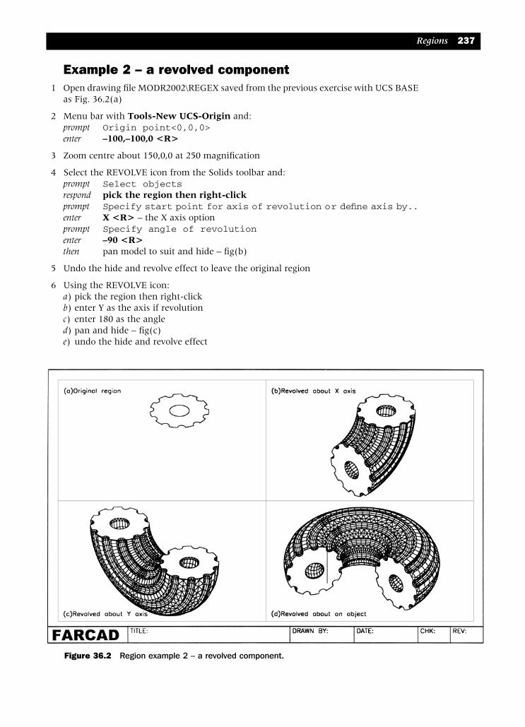
Example 2 – a revolved component1 Open drawing file MODR2002\REGEX saved from the previous exercise with UCS BASE
as Fig. 36.2(a)
2 Menu bar with Tools-New UCS-Origin and:prompt Origin point<0,0,0>enter –100,–100,0 <R>
3 Zoom centre about 150,0,0 at 250 magnification
4 Select the REVOLVE icon from the Solids toolbar and:prompt Select objectsrespond pick the region then right-clickprompt Specify start point for axis of revolution or define axis by..enter X <R> – the X axis optionprompt Specify angle of revolutionenter –90 <R>then pan model to suit and hide – fig(b)
5 Undo the hide and revolve effect to leave the original region
6 Using the REVOLVE icon:a) pick the region then right-clickb) enter Y as the axis if revolutionc) enter 180 as the angled) pan and hide – fig(c)e) undo the hide and revolve effect
Regions 237
Figure 36.2 Region example 2 – a revolved component.
modelling with AutoCAD.qxd 17/06/2002 15:41 Page 237
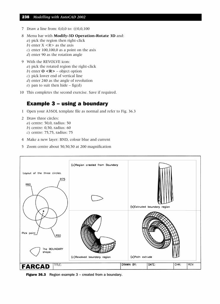
7 Draw a line from: 0,0,0 to: @0,0,100
8 Menu bar with Modify-3D Operation-Rotate 3D and:a) pick the region then right-clickb) enter X <R> as the axisc) enter 100,100,0 as a point on the axisd) enter 90 as the rotation angle
9 With the REVOLVE icon:a) pick the rotated region the right-clickb) enter O <R> – object optionc) pick lower end of vertical lined) enter 240 as the angle of revolutione) pan to suit then hide – fig(d)
10 This completes the second exercise. Save if required.
Example 3 – using a boundary1 Open your A3SOL template file as normal and refer to Fig. 36.3
2 Draw three circles:a) centre: 50,0, radius: 50b) centre: 0,50, radius: 60c) centre: 75,75, radius: 75
4 Make a new layer: BND, colour blue and current
5 Zoom centre about 50,50,50 at 200 magnification
238 Modelling with AutoCAD 2002
Figure 36.3 Region example 3 – created from a boundary.
modelling with AutoCAD.qxd 17/06/2002 15:41 Page 238
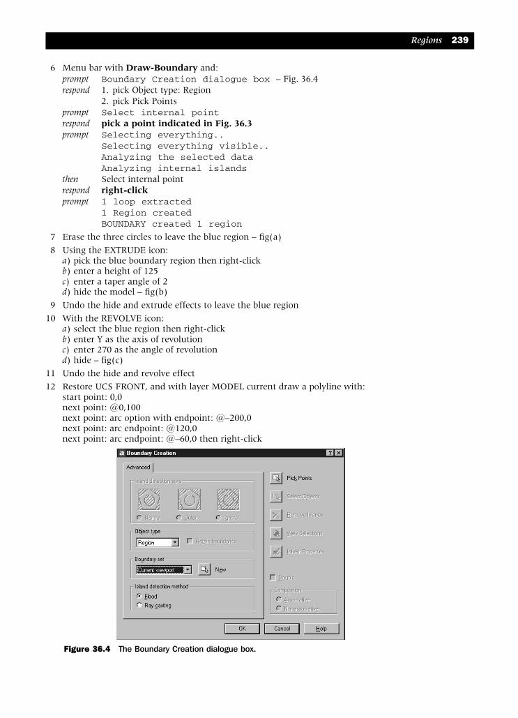
6 Menu bar with Draw-Boundary and:prompt Boundary Creation dialogue box – Fig. 36.4respond 1. pick Object type: Region
2. pick Pick Pointsprompt Select internal pointrespond pick a point indicated in Fig. 36.3prompt Selecting everything..
Selecting everything visible..Analyzing the selected dataAnalyzing internal islands
then Select internal pointrespond right-clickprompt 1 loop extracted
1 Region createdBOUNDARY created 1 region
7 Erase the three circles to leave the blue region – fig(a)
8 Using the EXTRUDE icon:a) pick the blue boundary region then right-clickb) enter a height of 125c) enter a taper angle of 2d) hide the model – fig(b)
9 Undo the hide and extrude effects to leave the blue region
10 With the REVOLVE icon:a) select the blue region then right-clickb) enter Y as the axis of revolutionc) enter 270 as the angle of revolutiond) hide – fig(c)
11 Undo the hide and revolve effect
12 Restore UCS FRONT, and with layer MODEL current draw a polyline with:start point: 0,0next point: @0,100next point: arc option with endpoint: @–200,0next point: arc endpoint: @120,0next point: arc endpoint: @–60,0 then right-click
Regions 239
Figure 36.4 The Boundary Creation dialogue box.
modelling with AutoCAD.qxd 17/06/2002 15:41 Page 239

13 Restore UCS BASE and make layer BND current
14 With the EXTRUDE icon:a) select the blue regionb) enter P <R> for the path optionc) pick the red polylined) pan to suitd) hide to give fig(d)
15 The exercise is complete, save?
16 NoteAlthough this exercise has been completed using the Boundary command, it could havealso been completed by making the three circles into regions and then using the Booleanintersection command.
Summary1 A region is created from closed shapes, e.g. polylines, arcs, circles, ellipses etc
2 Regions can be created with the BOUNDARY command
3 Regions consist of loops and all regions must have an outer loop. There can be severalinner loops.
4 Regions can be extruded and revolved
5 All parts of a region are extruded/revolved to the same height or angle
6 Regions are extruded along the Z-axis of the current UCS. The height of the extrusioncan be positive or negative
7 Regions can be extruded along a path
AssignmentThis activity requires a region to be created from circles, copied, scaled and then extrudedto different heights.
ACTIVITY 21: Ratchet mechanism of Macfaramus
While digging in a water bed outside the city of CADOPOLIS, a device was discoveredwhich was thought to be a ratchet mechanism for a primitive type of waterwheel. Thismechanism has three distinct ‘parts’ to it, each having the same shape.
Using the reference sizes given, create the outline from circles, convert these circles intoregions, then subtract the smaller circles from the larger. The other parts of themechanism are scaled by 0.85 and 0.55 from the original. When the three parts havebeen created, they have to be:a) lower part: extruded to a height of –50 with –15 taperb )middle part: extruded to a height of 60 with 0 taperc)top part: revolved about an line object for –90 degrees and then array for 3 items aboutthe top ‘circle’ centre. The line for the object can be drawn at your discretion. The lineI used is indicated in the activity drawing.
Notes:1 Use a 0,0 centre point for the large circle and for copying and scaling purposes2 Each scaled part is positioned on top of the previous part3 Use your discretion for sizes not given
240 Modelling with AutoCAD 2002
modelling with AutoCAD.qxd 17/06/2002 15:41 Page 240

Inquiring into modelsIn this chapter we will create two new composites and then use the AutoCAD inquirycommands to determine the properties of these solids. We will also investigate how tocreate a material properties file.
Composite model 4 – a slip block1 Open the A3SOL template file with normal settings, display the Inquiry toolbar and refer
to Fig. 37.1
2 Create the following primitives:Box Wedgecorner: 0,0,0 corner: 120,0,0length: 120 length: 50width: 100 width: 100height: 100 height: 70colour: red colour: blue
3 Centre the model about 80,50,50 at 200 magnification
Chapter 37
Figure 37.1 Composite model 4 – a slip block (plotted without hide).
modelling with AutoCAD.qxd 17/06/2002 15:41 Page 241

4 Create two green cylindrical primitives with:a) centre: 60,0,50
radius: 25centre of other end option: @0,100
b) elliptical optioncentre of ellipse: 0,50,50axis endpoint: @20,0length of other axis: @0,0,30centre of other end: @180,0
5 a) union the red box and blue wedgeb) subtract the two green cylinders from the compositec) note the ‘curves of interpenetration’d) shade and note the colour effecte) use the 3D orbit command with the model, then restore the original 2D wireframe
representation.
6 At this stage save the composite as MODR2002\SLIPBL
7 Select the AREA icon from the Inquiry toolbar and:prompt Specify first corner point or [Object/Add/Subtract]enter O <R> – the object optionprompt Select objectsrespond pick the compositeprompt Area = 98062.84, Perimeter = 0.00
9 The area value displayed is the surface area of the composite in square units (mm?). Asolid object has no perimeter, hence the 0 value
9 Select the REGION/MASS PROPERTIES icon from the Inquiry toolbar and:prompt Select objectsrespond pick the composite then right-clickprompt AutoCAD Text Windowwith details about the model including:
Mass = 995882.69Volume = 995882.69
prompt Write analysis to a file?<N>enter Y <R>prompt Create Mass and Area Properties File dialogue boxrespond 1. check – Save in: named folder active
2. check – Save as type *.mpr – materials properties3. enter File name: SLIPBL4. pick Save (more on properties file later)
10 Note that the mass and volume values are the same as AutoCAD 2002 assumes a densityof 1.
Composite model 5 – a casting block1 Close and existing drawings then open A3SOL template file with the normal settings and:
a) refer to Fig. 37.2b) zoom centre about 37,50,18 at 150 magnification in all viewports
2 With the 3D viewport active, create a box primitive with:a) corner: 0,0,0b) length: 75, width: 100, height: 36
242 Modelling with AutoCAD 2002
modelling with AutoCAD.qxd 17/06/2002 15:41 Page 242
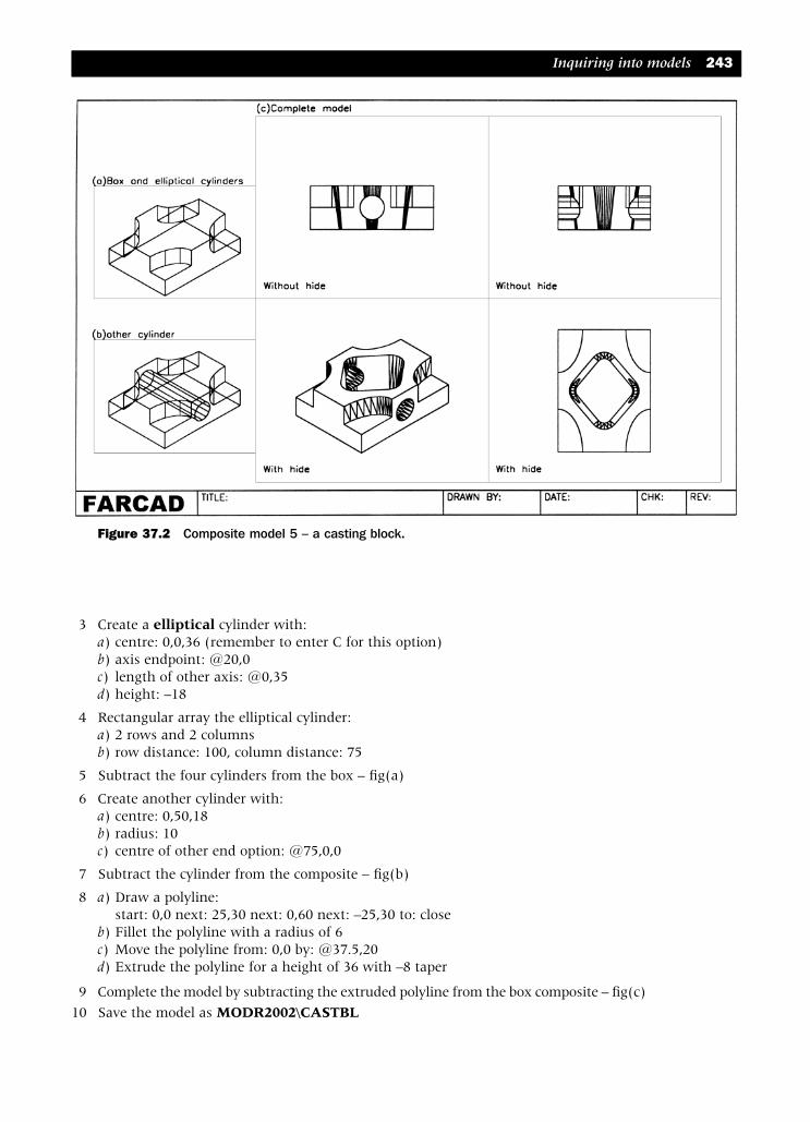
3 Create a elliptical cylinder with:a) centre: 0,0,36 (remember to enter C for this option)b) axis endpoint: @20,0c) length of other axis: @0,35d) height: –18
4 Rectangular array the elliptical cylinder:a) 2 rows and 2 columnsb) row distance: 100, column distance: 75
5 Subtract the four cylinders from the box – fig(a)
6 Create another cylinder with:a) centre: 0,50,18b) radius: 10c) centre of other end option: @75,0,0
7 Subtract the cylinder from the composite – fig(b)
8 a) Draw a polyline:start: 0,0 next: 25,30 next: 0,60 next: –25,30 to: close
b) Fillet the polyline with a radius of 6c) Move the polyline from: 0,0 by: @37.5,20d) Extrude the polyline for a height of 36 with –8 taper
9 Complete the model by subtracting the extruded polyline from the box composite – fig(c)
10 Save the model as MODR2002\CASTBL
Inquiring into models 243
Figure 37.2 Composite model 5 – a casting block.
modelling with AutoCAD.qxd 17/06/2002 15:41 Page 243
11 Menu bar with Format-Units and using the Drawing Units dialogue box alter:a) Length type: Engineeringb) Precision: 0’-0.00”c) Insert units: inchesd) pick OK
12 Select the AREA icon from the Inquiry toolbar and:a) use the object option and pick the compositeb) Area = 29416.67 square in (204.2824 square ft)
13 Select the MASS PROPERTIES icon, pick the composite and:prompt AutoCAD Text Windowwith Mass 155027.84 lb
Volume 155027.84 cu inrespond <RETURN> to the promptprompt Write Analysis to a file?<N>enter Y <R>prompt Create Mass and Area Properties File dialogue boxwith SLIPBL listed from previous exerciserespond 1. enter file name: CASTBL
2. pick Save
14 Investigatea) The area and mass properties have been ‘calculated’ with the UCS BASE. There are
two other UCS saved positions, FRONT and RIGHT. Using these saved UCS’s,determine the area and mass/ volume values with engineering units.My values were:UCS Area(sq in) Mass (lb)/Volume (cu in)BASE 29416.67 155027.84FRONT 29416.67 155029.90RIGHT 29416.67 155027.59These slight variations in mass/volume are due to the way in which AutoCAD 2002performs the various calculations.
b) Using the relevant commands, find the area and mass for the composite modelscreated in previous chapters. My values with UCS BASE and decimal units were:Model/chap Area MassMachine support(31) 81270.75 1022333.68Backing plate(32) 38171.70 98283.83Pipe/flange(33) 190938.19 1305275.35
Mass Properties fileWhen the mass properties command is used with a solid model, the AutoCAD Text Win-dow will display ‘technical’ information about the model including the mass and volume.
The user has the option of saving this information to a Mass Property file with theextension .mpr. As the mass property file is a ‘text file’ it can be opened in any ‘texteditor’ type package.
To demonstrate this:
1 Select the Windows Start icon from the Windows bar at the bottom of the screen thenselect Programs-Accessories-Notepad and:prompt Untitled Notepad screenrespond 1. menu bar with File-Open
2. at Look in, scroll and to named folder3. alter file name to *.mpr then <R>4. pick SLIPBL5. pick Open
2 The screen will display the saved material property file for the slip block composite –Fig. 37.3(a)
244 Modelling with AutoCAD 2002
modelling with AutoCAD.qxd 17/06/2002 15:41 Page 244
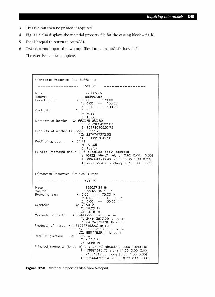
3 This file can then be printed if required
4 Fig. 37.3 also displays the material property file for the casting block – fig(b)
5 Exit Notepad to return to AutoCAD
6 Task: can you import the two mpr files into an AutoCAD drawing?
The exercise is now complete.
Inquiring into models 245
Figure 37.3 Material properties files from Notepad.
modelling with AutoCAD.qxd 17/06/2002 15:42 Page 245

Summary1 Mass properties can be obtained from solid models
2 The mass properties include mass, volume, centroid, radius of gyration etc.
3 The mass properties can be saved to an mpr text file
4 AutoCAD 2002 does not support a materials library and hence mass and volume arealways the same, as density is assumed to be 1.
AssignmentMACFARAMUS designed many different types of objects including garden walls andpaths. It is one of these ‘garden blocks’ that you now have to create as a solid model.The block was one of many used in the design of the famous walled gardens ofCADOPOLIS and the block was made from the mud of the river CLYDEBER on whosebanks CADOPOLIS was built.
Activity 22: Garden block of MACFARAMUS
The creation of the garden block is straightforward:
1 Open you template file as normal
2 Using the reference sizes in the activity drawing, create the model from primitives orregions – your choice
3 When the model is complete, save as MODR2002\GARDBL as it will be used in a laterchapter
4 Taska) when the model is complete, obtain the massb) MACFARAMUS obtained a quantity of mud from the banks of the river CLYDEBER
for making the blocks. If the mass of this mud was 1000000 units, how many blockscould he make (assuming no waste)
c) I worked out he could create 5748 blocks.
246 Modelling with AutoCAD 2002
modelling with AutoCAD.qxd 17/06/2002 15:42 Page 246
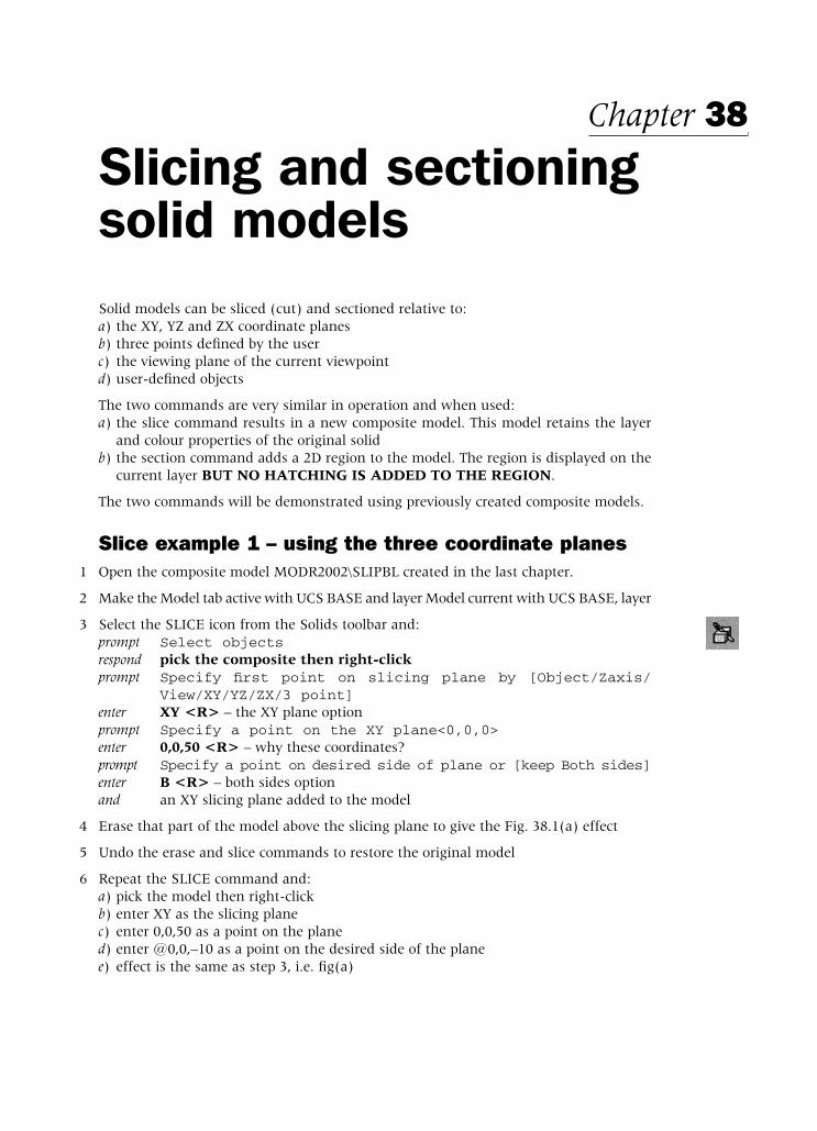
Slicing and sectioningsolid modelsSolid models can be sliced (cut) and sectioned relative to:a) the XY, YZ and ZX coordinate planesb) three points defined by the userc) the viewing plane of the current viewpointd) user-defined objects
The two commands are very similar in operation and when used:a) the slice command results in a new composite model. This model retains the layer
and colour properties of the original solidb) the section command adds a 2D region to the model. The region is displayed on the
current layer BUT NO HATCHING IS ADDED TO THE REGION.
The two commands will be demonstrated using previously created composite models.
Slice example 1 – using the three coordinate planes1 Open the composite model MODR2002\SLIPBL created in the last chapter.
2 Make the Model tab active with UCS BASE and layer Model current with UCS BASE, layer
3 Select the SLICE icon from the Solids toolbar and:prompt Select objectsrespond pick the composite then right-clickprompt Specify first point on slicing plane by [Object/Zaxis/
View/XY/YZ/ZX/3 point]enter XY <R> – the XY plane optionprompt Specify a point on the XY plane<0,0,0>enter 0,0,50 <R> – why these coordinates?prompt Specify a point on desired side of plane or [keep Both sides]enter B <R> – both sides optionand an XY slicing plane added to the model
4 Erase that part of the model above the slicing plane to give the Fig. 38.1(a) effect
5 Undo the erase and slice commands to restore the original model
6 Repeat the SLICE command and:a) pick the model then right-clickb) enter XY as the slicing planec) enter 0,0,50 as a point on the planed) enter @0,0,–10 as a point on the desired side of the planee) effect is the same as step 3, i.e. fig(a)
Chapter 38
modelling with AutoCAD.qxd 17/06/2002 15:42 Page 247

7 With the slice command, the user can either:a) specify a point on the desired side of the slicing plane to keep b) keep both models on either side of the slicing plane then erase or move one of them
8 Now undo the slice effect or re-open SLIPBL
9 Menu bar with Draw-Solids-Slice and:a) pick the composite then right-clickb) enter YZ <R> as the slicing planec) enter 50,0,0 <R> as a point on the planed) enter @–10,0,0 <R> to keep part ‘to left’ of slice planee) the new composite is created as fig(b)
10 Undo the slice effect
11 At the command line enter SLICE <R> and:a) pick the composite then right-clickb) enter ZX as the slicing planec) enter 0,50,0 as a point on the planed) enter @0,10,0 to keep part ‘below’ the slice planee) new composite as fig(c)
12 Undo the slice effect, activate the slice command and:a) pick the composite then right-clickb) select the YZ planec) enter 40,0,0 as a point on the planed) enter B <R> to keep both sidese) model is now ‘sliced’ into two new composites
248 Modelling with AutoCAD 2002
Figure 38.1 Slice example 1 – using the slicing planes with model SLIPBL.
modelling with AutoCAD.qxd 17/06/2002 15:42 Page 248

13 With the MOVE command:a) pick the blue wedge then right-clickb) base point: enter 170,0c) second point of displacement: enter @50,0d) the two new composites are separated – fig(d)
14 This completes the first exercise which does not need to be saved
Slice example 2 – using user-defined slicing planes1 Open the drawing file MODR2002\MACHSUPP – the first composite solid created in
chapter 31. Make the Model tab active with USC BASE and layer MODEL. Refer to Fig. 38.2
2 Activate the SLICE command and:prompt Select objectsrespond pick the composite then right-clickprompt Specify first point on slicing plane ..respond right-click/enter – accepting the 3 point defaultprompt Specify first point on plane and: ENDpoint icon and pick pt1prompt Specify second point on plane and: ENDpoint icon and pick pt2prompt Specify third point on plane and: QUAdrant icon and pick pt3prompt Specify a point on desired side of plane..enter @0,0,–10 <R> – why this entry?
3 A new composite will be created as fig(a). This has been ‘sliced’ through an inclinedplane.
Slicing and sectioning solid models 249
Figure 38.2 Slice example 2 – MABHSUPP using three-defined points.
modelling with AutoCAD.qxd 17/06/2002 15:42 Page 249
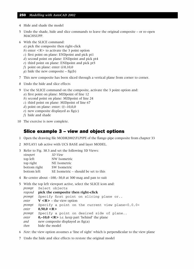
4 Hide and shade the model
5 Undo the shade, hide and slice commands to leave the original composite – or re-openMACHSUPP.
6 With the SLICE command:a) pick the composite then right-clickb) enter <R> to activate the 3 point optionc) first point on plane: ENDpoint and pick pt1d) second point on plane: ENDpoint and pick pt4e) third point on plane: ENDpoint and pick pt5f) point on plane: enter @0,10,0g) hide the new composite – fig(b)
7 This new composite has been sliced through a vertical plane from corner to corner.
8 Undo the hide and slice effects
9 Use the SLICE command on the composite, activate the 3 point option and:a) first point on plane: MIDpoint of line 12b) second point on plane: MIDpoint of line 24c) third point on plane: MIDpoint of line 67d) point on plane: enter: @–10,0,0e) new composite displayed as fig(c)f) hide and shade
10 The exercise is now complete.
Slice example 3 – view and object options1 Open the drawing file MODR2002\FLPIPE of the flange-pipe composite from chapter 33
2 MVLAY1 tab active with UCS BASE and layer MODEL.
3 Refer to Fig. 38.3 and set the following 3D Views:viewport 3D Viewtop left NW Isometrictop right NE Isometricbottom right SW Isometricbottom left SE Isometric – should be set to this
4 Re-centre about –100,–30,0 at 300 mag and pan to suit
5 With the top left viewport active, select the SLICE icon and:prompt Select objectsrespond pick the composite then right-clickprompt Specify first point on slicing plane or..enter V <R> – the view optionprompt Specify a point on the current view plane<0,0,0>enter 0,50,0 <R>prompt Specify a point on desired side of plane..enter 0,–10,0 <R> i.e. keep part ‘behind’ the planeand new composite displayed as fig(a)then hide the model
6 Note: the view option assumes a ‘line of sight’ which is perpendicular to the view plane
7 Undo the hide and slice effects to restore the original model
250 Modelling with AutoCAD 2002
modelling with AutoCAD.qxd 17/06/2002 15:42 Page 250

8 With the top right viewport active, SLICE and:a) pick the composite then right-clickb) enter V <R> for the view optionc) enter 0,50,0 <R> as a point on the view planed) enter 0,–10,0 <R> as a point on the desired side on the planee) new composite createdf) hide the model – fig(b)
9 Undo the hide and slice effects
10 Make the lower right viewport active and slice with:a) the compositeb) the view optionc) 0,–50,0 as a point on the planed) 0,10,0 as a point on the desired side of the planee) new composite as fig(c)f) hide then undo both the hide and slice effects
11 Finally with the lower left viewport active:a) draw a circle with centre: 0,–100 and radius: 100b) rotate 3D this circle:
1. about the X axis2. with the circle centre as a point on the axis3. for a reference angle of 45 degrees
c) with the SLICE command:1. pick the composite then right click2. enter O <R> for the object option3. pick the circle as the object4. enter 0,10,0 as a point on desired side5. erase the circle then hide and composite as fig(d)
The slice examples have now been completed.
Slicing and sectioning solid models 251
Figure 38.3 Slice example 3 – FLPIP model with view and object options.
modelling with AutoCAD.qxd 17/06/2002 15:42 Page 251

Section example – three point optionThe section command is very similar in operation to the slice command, and only oneexample will be demonstrated
1 Open the drawing file MODR2000\SLIPBL from chapter 37, MVLAY1 tab, UCS BASE,layer MODEL and the lower left viewport active. Refer to Fig. 38.4
2 Make layer SECT current – or make a new section layer
3 Select the SECTION icon from the Solids toolbar and:prompt Select objectsrespond pick the composite then right-clickprompt Specify first point on section plane by..respond <R> – to activate the three point optionprompt Specify first point on plane and ENDpoint of pt1prompt Specify second point on plane ENDpoint of pt2prompt Specify third point on plane pick ENDpoint of pt3
4 A coloured outline as added to the model
5 Menu bar with Tools-Inquiry-List and:prompt Select objectsrespond pick any point on the added outline then right-clickprompt AutoCAD Text Windowwith details about the selected object and it is a REGIONrespond cancel the text window
252 Modelling with AutoCAD 2002
Figure 38.4 Section example with model SLIPBL plotted without hide.
modelling with AutoCAD.qxd 17/06/2002 15:42 Page 252

6 Notea) Hatching is not automatically added to the regionb) Hatching must be added to the section region by the user.c) The section region is displayed in all viewports, and the viewport specific layer concept
can then be used to ‘currently freeze’ the section outline in specific viewports.d) If hatching is to be added to the section region (as it should?), remember to alter the
UCS position as hatching is a 2D concept
7 TaskAdd hatching to the added section plane using the following information:a) Hatching to be Predefined-ANSI-ANSI33b) Scale: 1 and Angle: 0c) Hide the model in each viewport with interesting resultsd) A new 3-point UCS will be required and the points should be obvious, as they are the
same as the section plane points
8 In a later chapter we will section models ‘more realistically’
Using the slice and section commandsIf a ‘true section’ has to be obtained from a solid composite, then the slice and sectioncommands can both be used. To demonstrate this concept:
1 Open drawing file MODR2002\CASTBL from chapter 37 with MVLAY1 tab, UCS BASE,layer MODEL and the lower left viewport active.
2 Refer to Fig. 38.5 which displays the original model in fig(a)
Slicing and sectioning solid models 253
Figure 38.5 Using the SLICE and SECTION commands with CASTBL.
modelling with AutoCAD.qxd 17/06/2002 15:42 Page 253

3 With the SLICE command:a) pick the composite then right-clickb) use the three points on slicing plane option and pick the ENDpoints of points 1,2
and 3c) enter 0,100,0 as the point on the desired side on the planed) a new composite will be displayed
4 With layer SECT current, use the SECTION command and:a) pick the new composite then right-clickb) use the three point options with the same selection as step 3c) region added to composite
5 Hatch the region with correct UCS setting
6 Fig. 38.5(b) displays the result of the SLICE and SECTION commands
Summary1 The SLICE command produces a new composite on the same layer as the original model
2 The SECTION command adds a region to the section plane of the model, but does notadd any hatching to this region. Hatching must be added by the user and is UCSdependent
3 Both commands are very similar with the following options:a) the XY, YZ and ZX slicing/sectioning planesb) defining any three points on the slice/section planec) relative to an objectd) relative to the viewing plane in the current viewpoint
4 The SLICE command requires:a) a point on the slicing planeb) a point on the desired side of the plane which is to ‘be kept’
5 The SECTION command only requires a point on the sectioning plane
6 The orientation of the UCS will affect the XY,YZ and ZX planes
7 The two commands can be activated:a) by icons from the Solids toolbarb) from the menu bar with Draw-Solidsc) by entering SLICE or SECTION from the keyboard.
254 Modelling with AutoCAD 2002
modelling with AutoCAD.qxd 17/06/2002 15:42 Page 254

Profiles and trueshapesWhen the HIDE command is used with a solid composite, the model is displayed withhidden line removal – as expected. From an ‘engineering viewpoint’ this may not be whatis wanted, as the front, top and end views should have lines which represent hiddendetail. AutoCAD 2002 allows this hidden detail to be ‘added’ to a solid model with thePROFILE command and when used, new layers are automatically added to the existingdrawing.
A profile is defined as: an image which displays the edges and silhouettes of curved
surfaces of the solid for the current view
The command will be demonstrated with previously created models.
Example 1 – slip block1 Open drawing MODR2002\SLIPBL from chapter 37.
2 In paper space, use the LIST command and pick the top right viewport border. TheAutoCAD Text Window will display information about the viewport including theHANDLE number. Take a note of this handle number, then repeat the LIST commandselecting the other three viewport borders. In each case note the handle number as itwill be referred to in the exercise. My handle numbers for the four viewports were:top right: 70 top left: 72lower right: 76 lower left: 74
3 Note:a) all objects created in AutoCAD are given a handle number and this number increases
every time a new object is added to the drawingb) the handle numbers are in hexadecimal format – don’t worry about this if you have
never heard of it. It is not important at this level of AutoCADc) the handles are for assisting with the AutoCAD databased) your four viewport handle numbers will probably differ from mine. This is perfectly
normal. Simply note them.
4 After the viewport border handle numbers have been noted, return to model space withUCS BASE.
5 Make layer 0 current and the top left viewport active.
6 Refer to Fig. 39.1
Chapter 39
modelling with AutoCAD.qxd 17/06/2002 15:42 Page 255

7 Select the SETUP PROFILE icon from the Solids toolbar and:prompt Select objectsrespond pick the composite then right-clickprompt Display hidden profile lines on a separate layer?[Yes/No]<Y>enter Y <R>prompt Project profile lines onto a plane?[Yes/No]<Y>enter Y <R>prompt Delete tangential edges?{Yes/No]<Y>enter Y <R>and the model in the top left viewport will be displayed with black lines over the
model lines
8 Menu bar with Format-Layer and:prompt Layer Properties Manager dialogue boxwith two new layers (*):
a) PH-72 for hidden profile lines – Hidden linetype?b) PV-72 for visible profile lines – Continuous
respond 1. check the linetype for layer PH-722. if it is not Hidden, then LOAD the HIDDEN linetype and set it to layer PH-
723. freeze layer MODEL in the current viewport4. pick OK
9 The two new layers (*) will have the same handle number as the top left viewport, inmy case 72
10 The top left viewport will now only display the profile visible and hidden lines for thecomposite as layer MODEL has been frozen in the current viewport. Do you understandwhy the linetype for layer PH-72 was set to HIDDEN?
256 Modelling with AutoCAD 2002
Figure 39.1 Using the PROFILE command with SLIPBL.
modelling with AutoCAD.qxd 17/06/2002 15:42 Page 256

11 Make the top right viewport active and from the menu bar select Draw-Solids-Setup-Profile and:prompt Select objectsrespond pick the composite then right-clickprompt Display hidden profile lines.. and <R>prompt Project profile lines.. and <R>prompt Delete tangential edges.. <R>
12 The model will be displayed with black visible and hidden lines13 Menu bar with Format-Layer and:
prompt Layer Properties Manager dialogue boxwith Two new layers:
a) PH-70 with HIDDEN linetypeb) PV-70 with CONTINUOUS linetype
respond 1. freeze layer MODEL in current viewport2. pick OK
and a) remember that PH-70 and PV-70 are the visible and hidden layers for myviewport handles. You may have different PH and PV handle numbers
b) layer PH-70 has HIDDEN linetype as this linetype was loaded in step 8
14 The top right viewport will display visible and hidden lines for the model.
15 Make the lower right viewport active, still with layer 0 current
16 At the command line enter SOLPROF <R> and:a) pick the model then right-clickb) enter Y <R> to the display hidden profile lines promptc) enter Y <R> to the project profile lines promptd) enter Y <R> to the delete tangential edges prompte) layer properties manager dialogue box and:
1. two new layers: PH-76 and PV-762. freeze layer MODEL in current viewport3. pick OK
17 The viewport will display the visible and hidden detail lines for the model in the viewport18 At this stage the layout should resemble Fig. 39.1 and can now be saved if required, but
not as SLIPBL.This exercise is now complete.
ExplanationThe PROFILE command is viewport specific and when activated:
1 Two viewport specific layers are automatically created, these being PH-?? and PV-??
2 The PH layer is for hidden detail
3 The PV layer is for visible detail
4 The ?? with the layer name is the current viewport handle number and is not controlledby the user
5 The PV linetype should always be continuous
6 The PH linetype should always be hidden, but MAY HAVE TO BE LOADED by the user
7 The command must be used in each viewport in which profile detail has to be extracted
8 The command is generally used in viewports which display top, front and side views ofthe model
9 The command is generally not used in a viewport which displays a 3D view of the model
10 The hidden and visible detail added are blocks, i.e. there is a hidden detail block and avisible detail block. These blocks can be exploded if required.
Profiles and true shapes 257
modelling with AutoCAD.qxd 17/06/2002 15:42 Page 257

Example 2 – the pipe and flange1 Open the pipe/flange model created in chapter 33 with MVLAY1 tab, UCS BASE, layer
MODEL, lower left viewport active and refer to Fig. 39.2
2 In the top left viewport, activate the PROFILE command and:a) pick the model then right-clickb) enter Y <R> to the three promptsc) activate the Layer Properties Manager dialogue box and:
1. load the HIDDEN linetype and set to the new PH layer2. freeze layer MODEL in the current viewport
3 Repeat step 2 in the top right and lower right viewports, but do not load the HIDDENlinetype – it is already loaded?
4 Extracting profiles is as simple as this!
5 Profile drawings can be dimensioned using viewport specific layers using the sameprocedure as chapter 25. I will let you try and add the dimensions for yourself, butremember to:a) create a new layer for each viewportb) set the correct UCS – dimensioning is a 2D concept.
6 Save the layout when complete.
258 Modelling with AutoCAD 2002
Figure 39.2 The PROFILE command with the flange/pipe model.
modelling with AutoCAD.qxd 17/06/2002 15:42 Page 258

Profile explanationWhen the profile command is used with a solid model, three prompts are displayed andit is usual to enter Y to these prompts.a) Display hidden profile lines on separate layers
This creates two blocks, one for visible lines and one for hidden lines. Two newviewport specific layers are created for this block information PH-?? and PV-??. Theactual ?? number is the handle of the current viewport, i.e. it is unique. The PV (visibledetail) has a continuous linetype, while the PH (hidden detail) has a hidden linetype.The hidden linetype must be loaded before it can be ‘assigned’ to the PH layer
b) Project profile lines onto a planeThe profile detail is displayed as 2D objects and is projected onto a planeperpendicular to the viewing direction and passing through the UCS origin
c) Delete tangential edgesA tangential edge is an imaginary edge where two faces meet at a tangent. Tangentialedges are not shown for most drawing applications.
TRUE SHAPESA true shape is obtained when a surface (face) is viewed at right angles. In AutoCAD2002 this can be obtained with the PLAN and Solids Editing commands. We will use amodel from a previous chapter to demonstrate how a true shape can be obtained.
1 Open the machine support model from chapter 31 and refer to Fig. 39.3.
Profiles and true shapes 259
Figure 39.3 True shape extraction using composite model 1.
modelling with AutoCAD.qxd 17/06/2002 15:42 Page 259

2 In the top two viewports, use the PROFILE command and:a) accept the three Y promptsb) freeze layer MODEL in these two active viewportsc) load linetype HIDDEN and set to the two new PH layers
3 Create a new layer TS, colour to suit and current
4 With the lower right viewport active, restore UCS SLOPE which should have been savedwith the model during the chapter 31 exercise
5 Menu bar with View-3D Views-Plan View-Current UCS to display the sloped surfaceof the model as a ‘true shape’
6 Menu bar with Modify-Solids Editing-Copy faces and:prompt Select objectsrespond pick any pt 1 within the sloped face then right-click and enter (toggle
between the two lower viewports)prompt Specify a base point and enter: 0,0 <R>prompt Specify a second point of displacement and enter: @0,0,10 <R>
7 a) freeze layer MODEL in the current (lower right) viewport to display the true shapeof the sloped surface
b) making each of the other viewports active, freeze layer TS in the other three currentviewports
c) make the lower right viewport active, still with UCS SLOPE
8 Menu bar with Modify-Rotate and:prompt Select objectsrespond pick any point on the true shapeprompt Specify base point and enter: 0,0 <R>prompt Specify rotation angle and enter: –45 <R>
9 The true shape is rotated and now has to be positioned relative to the sloped surface‘from which it was copied’
10 In the lower right viewport, zoom extents the zoom 1.5 to ‘scale’ the true shape to thesame ‘value’ as the model
11 In paper space, activate the MOVE command and:prompt Select objectsrespond pick any point on the lower right viewport border then right-clickprompt Specify base point or displacementrespond Endpoint icon and pick pt aprompt Specify second point of displacementrespond Endpoint icon and pick pt b
12 Repeat the MOVE command with:a) objects: pick the moved viewport borderb) base point: endpoint icon and pick pt bc) second point: enter @170<–45
13 The true shape is moved to another part of the screen
14 Taska) dimension the true shape with the correct UCS and layer. This layer will need to be
currently frozen in the other viewportsb) freeze the layer VP to give the layout as Fig. 39.3
15 The exercise is now complete and should be saved as it will be used in the next chapter.
260 Modelling with AutoCAD 2002
modelling with AutoCAD.qxd 17/06/2002 15:42 Page 260

Summary1 Profiles can be extracted from models
2 Profiles display views of solid models with visible and hidden details
3 New layers are created with the PROFILE command, PV for visible objects and PH forhidden objects
4 The PH and PV layers are not controlled by the user and are assigned handle numbers.These handle numbers are those of the viewport in which the profile was extracted.
5 True shapes can be extracted from models with the copy faces solids editing command.
Profiles and true shapes 261
modelling with AutoCAD.qxd 17/06/2002 15:42 Page 261
Dimensioning inmodel and paperspaceAll users will know that AutoCAD has two drawing environments, these being:a) model space: used to create the modelb) paper space: used to layout the drawing sheet for plotting
When a multiple viewport layout has been created in paper space and dimensions haveto be added to the ‘model’, many users are unsure whether these dimensions should beadded in model space or paper space. In this chapter we will investigate both model andpaper space dimensioning.
We will use a previously created model for the demonstration.
Getting started1 Open the SLIPBL model from chapter 37 with MVLAY1 tab active
2 In model space with the top left viewport active:a) set a FRONT 3D viewb) zoom extents then zoom at 1.5 scalec) extract a profile of the modeld) load linetype HIDDEN if requirede) freeze layer Model in the current viewport
3 Repeat step 2 in the top right and lower right viewports
4 You should now have the same view in three viewports
5 Refer to Fig. 40.1, restore UCS FRONT and make layer DIM current
6 If you have the ability, modify the 3DSTD dimension style to increase the text height to 6. This is not greatly important
7 Linear dimension the top line of the model and diameter dimension the circle. Thesetwo dimensions will be displayed in all four viewports, as dimensioning is global.
8 Erase these two dimensions
Chapter 40
modelling with AutoCAD.qxd 17/06/2002 15:42 Page 262
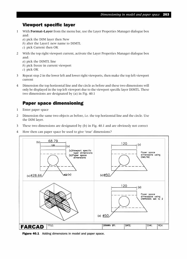
Viewport specific layer1 With Format-Layer from the menu bar, use the Layer Properties Manager dialogue box
and:a) pick the DIM layer then Newb) alter the Layer1 new name to DIMTLc) pick Current then OK
2 With the top right viewport current, activate the Layer Properties Manager dialogue boxand:a) pick the DIMTL lineb) pick freeze in current viewportc) pick OK
3 Repeat step 2 in the lower left and lower right viewports, then make the top left viewportcurrent
4 Dimension the top horizontal line and the circle as before and these two dimensions willonly be displayed in the top left viewport due to the viewport specific layer DIMTL. Thesetwo dimensions are designated by (a) in Fig. 40.1
Paper space dimensioning1 Enter paper space
2 Dimension the same two objects as before, i.e. the top horizontal line and the circle. Usethe DIM layer.
3 These two dimensions are designated by (b) in Fig. 40.1 and are obviously not correct
4 How then can paper space be used to give ‘true’ dimensions?
Dimensioning in model and paper space 263
Figure 40.1 Adding dimensions in model and paper space.
modelling with AutoCAD.qxd 17/06/2002 15:42 Page 263

Using DIMLFACDIMLFAC (Dimension Linear scale Factor) is a system variable which when set to thecorrect value will scale linear and radial measurements and allow paper spacedimensioning of model space objects to have the ‘correct’ value.
1 In model space make the top right viewport active, then enter paper space
2 At the command line enter DIM <R> and:prompt Dim:enter DIMLFAC <R>prompt Enter new value for dimension variable, or Viewportenter V <R> – the viewport optionprompt Select viewport to set scalerespond pick the border of the top right viewportprompt DIMLFAC set to –1.74449then Dim:respond ESC to end the command line dimension sequence
3 Still in paper space, dimension the same linear and circular objects in the top rightviewport. The dimensions should now be correct, designated by (c)
Using DIMASSOCDIMASSOC is a system variable which controls dimension associativity, i.e. its valuedetermines whether any added dimension will change when the object it is associatedwith is changed. DIMASSOC can have one of three values as follows:a) 0 : dimensions are displayed exploded, i.e. any part of the dimension can be selectedb) 1 : the complete dimension is a single object and model space associativity applies.
This is the normal default valuec) 2 : the complete dimension is a single object and paper space associativity applies
1 Paper space still active
2 At the command line enter DIMLFAC <R> and:prompt Enter new value for DIMLFAC<–1.7445>enter 1 <R>
3 At the command line enter DIMASSOC <R> and:prompt Enter new value for DIMASSOC<?> – probably 1 valueenter 2 <R>
4 Now dimension the two objects as before using the lower right viewport. The dimensionsshould be correct, as (d)
5 This exercise is now complete and need not be saved.
264 Modelling with AutoCAD 2002
modelling with AutoCAD.qxd 17/06/2002 15:42 Page 264

Paper space dimension exercise1 Open the profile drawing saved in the previous chapter and refer to Fig. 40.2
2 With command line entry, set DIMLFAC to 1 and DIMASSOC to 2
3 Enter paper space and add the linear and circular dimensions
4 Are these paper space dimensions correct?
5 Enter model space with layer TS current and make viewport with the true shape active
6 Copy the true shape to another part of the viewport – you may have to ‘paper space’stretch this viewport
7 Explode the copied shape
8 In paper space, with layer DIM current, align dimension the 100 line and diameterdimension the circle
9 Enter model space and:a) activate the scale commandb) window the true shapec) pick a suitable base pointd) enter a scale factor of 1.2
10 The model space shape and the paper space dimensions should both be scaled by 1.2
11 This is true associativity, i.e. paper space dimensions are associated with model spaceobjects.
This exercise is complete and can be saved.
Dimensioning in model and paper space 265
Figure 40.2 Paper space dimension exercise.
modelling with AutoCAD.qxd 17/06/2002 15:42 Page 265

Summary1 Dimension can be added to models in both model and paper space
2 Multiple viewport model space dimensioning requires viewport specific layers to be madeby the user
3 Paper space dimensions can be added to multiple viewport models by setting theDIMLFAC system variable
4 True associative paper space dimensions can be added to models in a multiple viewportlayout with the DIMASSOC system variable set to 2. This is the recommended method.
AssignmentThis activity requires the garden block from the previous activity to be dimensioned.
Activity 23: Adding dimensions to the garden block of MACFARAMUS.
1 Open your activity 22
2 Set DIMASSOC to 2
3 Extract profiles from the top and front views then currently freeze the model layer inthese viewports
4 Add suitable paper space dimensions to the model layout
5 Extract a diagonal section through the block and hatch using the AR-CONC predefinedpattern at a suitable scale
6 Save with a suitable name
266 Modelling with AutoCAD 2002
modelling with AutoCAD.qxd 17/06/2002 15:42 Page 266
A detailed drawingIn this example a new composite will be created and used to display the model as adetailed drawing. The model to be created is a desk tidy, so open your A3SOL templatefile with MVLAY1 tab active, UCS BASE, layer MODEL, lower left viewport active.
Altering the viewports1 In paper space select the STRETCH icon from the Modify toolbar and:
prompt Select objectsenter C <R> – the crossing optionprompt Specify first corner and enter: 160,100 <R>prompt Specify opposite corner and enter: 260,200 <R>prompt 4 found, Select objectsrespond right-clickprompt Specify base point or displacement and enter: 200,135 <R>prompt Specify second point of displacement and enter: @–25,25 <R>
2 The viewport configuration will be altered
3 Return to model space with UCS BASE
The basic shape1 Refer to Fig. 41.1
2 With the lower left viewport active restore UCS FRONT
3 Draw a polyline using the following entries:Start point: 0,0 next point: @156,0 next point: @0,15next point: @–132,0 next point: @0,10 next point: @–24,0next point: close
4 With the EXTRUDE icon from the Solids toolbar, extrude the red polyline with:a) height: –85b) taper: 0
5 Restore UCS BASE and zoom centre about the point 78,42,8 at 0.9XP in the 3D viewportand 1XP in the other three viewports. The XP entry is to allow for the different viewportsizes, i.e. the model is being zoomed about a centre point relative to the size of theviewport.
6 The extruded polyline will be displayed as fig(a)
Chapter 41
modelling with AutoCAD.qxd 17/06/2002 15:42 Page 267

The top1 Create a box primitive with:
a) corner: 0,12,25b) length: 6; width: 61; height: 5
2 Create three wedges using the following information:a) corner: 6,12,25; length: 18; width: 61; height: 5b) corner: 6,12,25; length: 12; width: –6; height: 5c) corner: 6,73,25; length: 12; width: 6; height: 5
3 With the ROTATE icon, rotate the following wedges:1. wedge (b) about the point 6,12,25 by –902. wedge (c) about the point 6,73,25 by 90
4 Union the box and the three wedges with the red extrusion5 The model at this stage resembles fig(b)6 Create another two wedges with:
a) corner: 6,0,25; length: 18; width: 12; height: 5b) corner: 24,12,25; length: 12; width: –18; height: 5
7 Rotate the second wedge (b) about the point 24,12,25 by –908 Menu bar with Modify-Solids Editing-Intersect and:
prompt Select objectsrespond pick the two wedges then right-click
9 Menu bar with Modify-3D Operation-Mirror 3D and:prompt Select objectsrespond pick the intersected wedges then right-clickprompt Specify first point of mirror plane or..enter ZX <R> – the ZX plane optionprompt Specify point on ZX planeenter 0,42.5,25 <R>prompt Delete source objects?<N> and enter: N <R>
10 Union the two sets of intersected wedges with the composite
11 The model should be displayed as fig(c)
268 Modelling with AutoCAD 2002
Figure 41.1 Steps in the construction of the desk tidy (3D view only with hide).
modelling with AutoCAD.qxd 17/06/2002 15:42 Page 268

The compartments1 The desk tidy compartments will be created from boxes subtracted from the composite.
2 With lower left viewport active and UCS BASE, create the following four box primitives:box1 box2 box3 box4
corner 153,3,3 100,3,3 100,36,3 100,52,3length –50 –76 –76 –76width 79 30 13 30height 20 20 20 20colour magenta blue green blue
3 Subtract the four boxes from the red composite – fig(d)
5 Shade the model in the 3D viewport then return to 2D wireframe representation
The end cut-out1 Lower left viewport active with UCS BASE
2 Set a new UCS position with the 3 point option using:a) origin: 156,0,0b) x-axis position: 156,85,0c) y-axis position: 156,0,15d) save UCS position as NEWEND
3 Draw a polyline with the following keyboard entries:Start point: 10,15Next point: @0,–3Next point: arc option with arc endpoint: @3,–3Next point: line option with line endpoint: @59,0Next point: arc option with arc endpoint: @3,3Next point: line option with line endpoint: @0,3Next point: close
4 Set ISOLINES to 6 and FACETRES to 0.5
5 Extrude the polyline for a height of –3 with 0 taper
6 Subtract the extruded polyline from the composite – fig(e)
7 Restore UCS BASE
The holes on the slope1 In paper space zoom in on the 3D sloped area then model space
2 Set a new UCS position with the 3 point option using:a) origin: 24,42.5,25b) x-axis position: 24,85,25c) y-axis position: 6,42.5,30d) save UCS position as SLOPE
A detailed drawing 269
modelling with AutoCAD.qxd 17/06/2002 15:42 Page 269

3 Create three cylinders, colour magenta with:cylinder 1 cylinder 2 cylinder 3
centre 0,9.34077,0 20,9.34077,0 –20,9.34077,0radius 3 5 5height –12 –20 –20
4 Subtract the three cylinders from the red composite – fig(f)
5 In paper space, zoom previous and return to model space
The complete model1 Restore UCS BASE
2 The model is now complete and your screen display should be similar to Fig. 41.2
3 Save the model at this stage as MODR2002\DESKTIDY
4 In the 3D viewport use the 3D orbit command with Gouraud shading then return theoriginal view as wireframe
Extracting a profile1 Refer to Fig. 41.3 and with the top left viewport active, select the SETUP PROFILE icon
from the Solids toolbar and:prompt Select objectsrespond pick the composite then right-clickprompt Display hidden profile lines.. and enter: Y <R>prompt Project profile line.. and enter: Y <R>prompt Delete tangential edges and enter: Y <R>
270 Modelling with AutoCAD 2002
Figure 41.2 Complete desk tidy model.
modelling with AutoCAD.qxd 17/06/2002 15:42 Page 270

3 The model will be displayed with black lines
4 Using the Layer Properties Manager dialogue box:a) note new layers PH?? and PV?? b) load the linetype HIDDEN (if required) and set the new PH?? layer with this linetypec) freeze layer MODEL in this active viewport
Extracting the section1 With the top right viewport active, ensure UCS BASE and make layer SECT current
2 With the SECTION icon from the Solids toolbar:a) pick the composite then right-clickb) enter ZX as the section planec) enter 0,42,5,0 as a point on the planed) a region will be displayed in all viewports
3 a) currently freeze layer MODEL in the top right viewportb) currently freeze layer SECT in the other three viewports
4 With an appropriate UCS setting, add hatching to the region using: pattern name:ANSI32; scale: 1; angle: 0
Extracting the true shape1 The layout on your screen at present will differ from Fig. 41.3 so in paper space use the
MOVE command to interchange the viewports, i.e. the two lower viewports to the topof the paper sheet and the two top viewports to the bottom of the sheet. Use the endpointicon and pick a viewport border corner
2 Make a new layer named TS, colour to suit and current
3 In the top left and the two lower viewports, freeze the new layer TS in these activeviewports
4 With the top right viewport active, restore UCS SLOPE
5 Menu bar with Modify-Solids Editing-Copy faces and:prompt Select facesrespond pick any point within the sloped face indicated by pt 1 in the top left
viewport then right-click/enterprompt Specify a base point and enter: 0,0,0 <R>prompt Specify a second point and enter: @0,0,0 <R>prompt Enter a face editing option and enter: X <R> and X <R>
6 The face has been copied ‘on to itself’
7 Now currently freeze layer MODEL in the top right viewport to display the coloured trueshape of the sloped surface
8 Menu bar with View-3D Views-Plan View-Current UCS to display the copied face(true shape) in plan view. The position of this plan view may not be ideal
9 With the ROTATE icon from the MODIFY toolbar:a) pick the shape and <R>b) enter 0,0 as the base pointc) enter 74.476 as the rotation angle – this angle should become apparent once thedimensions have been added
A detailed drawing 271
modelling with AutoCAD.qxd 17/06/2002 15:42 Page 271
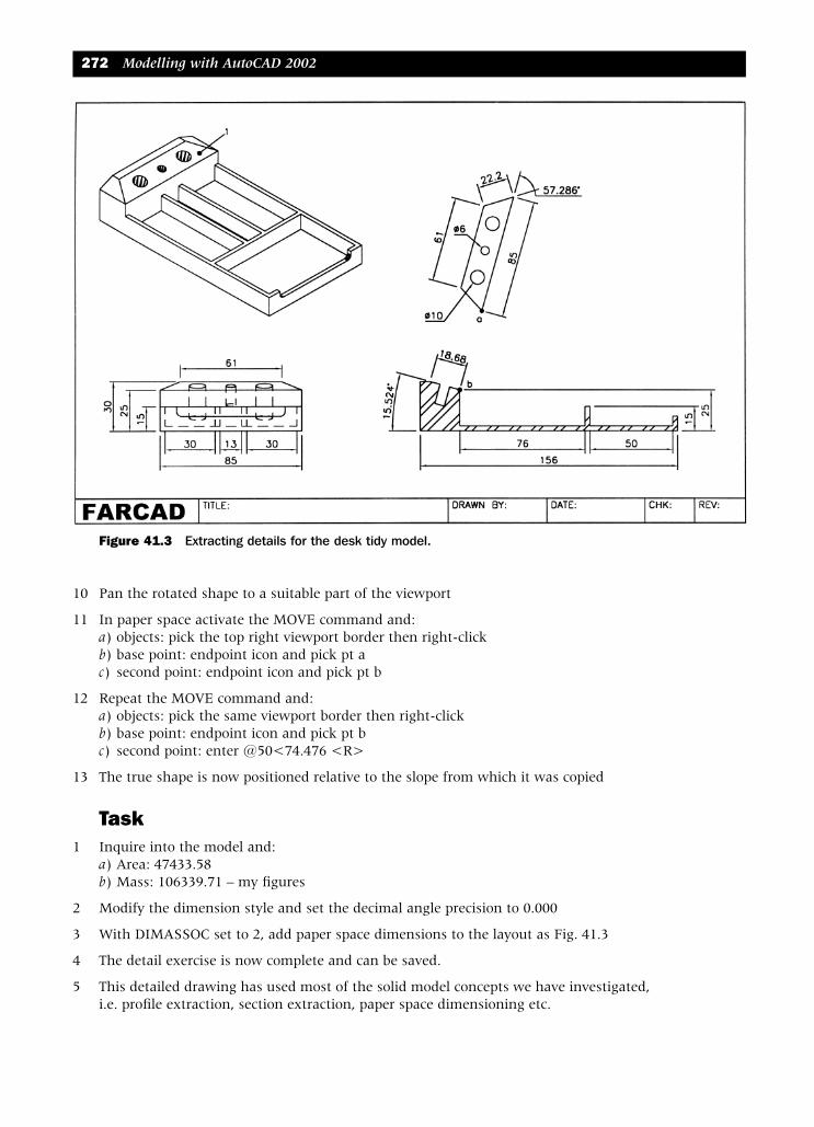
10 Pan the rotated shape to a suitable part of the viewport
11 In paper space activate the MOVE command and:a) objects: pick the top right viewport border then right-clickb) base point: endpoint icon and pick pt ac) second point: endpoint icon and pick pt b
12 Repeat the MOVE command and:a) objects: pick the same viewport border then right-clickb) base point: endpoint icon and pick pt bc) second point: enter @50<74.476 <R>
13 The true shape is now positioned relative to the slope from which it was copied
Task1 Inquire into the model and:
a) Area: 47433.58b) Mass: 106339.71 – my figures
2 Modify the dimension style and set the decimal angle precision to 0.000
3 With DIMASSOC set to 2, add paper space dimensions to the layout as Fig. 41.3
4 The detail exercise is now complete and can be saved.
5 This detailed drawing has used most of the solid model concepts we have investigated,i.e. profile extraction, section extraction, paper space dimensioning etc.
272 Modelling with AutoCAD 2002
Figure 41.3 Extracting details for the desk tidy model.
modelling with AutoCAD.qxd 17/06/2002 15:42 Page 272

Blocks, wblocks andexternal referencesSolid model blocks and wblocks can be created and inserted into drawings like any other2D or 3D object. In this chapter we will create two interesting (I hope) solid modelassembly drawings from blocks and wblocks and then investigate solid model externalreferences. We will also investigate the ‘interference’ between solids.
Example 1 – a desk tray assembly1 Open your A3SOL template file with the MVLAY1 tab as normal and refer to Fig. 42.1
2 Zoom centre about 55,40,20 at 0.75XP in all viewports
3 Set the ISOLINES system variable to 8 and FACETRES to 0.5
Figure 42.1 Creation of the assembled model.
Chapter 42
modelling with AutoCAD.qxd 17/06/2002 15:42 Page 273

The Tray1 Make a new layer TRAY, colour blue and current
2 With UCS BASE, create two primitives from:Box Cylindercorner: 0,0,0 centre: 10,0,0length: 110 radius: 10width: 80 height: 40height: 40
2 Rectangular array the cylinder:a) for 2 rows and 2 columnsb) row distance: 80 and column distance: 70
3 Union the box and the four cylinders – fig(a)
4 Create another two primitives from:Box Wedgecorner: 10,10,10 corner: 110,0,40length: 110 length: –15width: 60 width: 80height: 40 height: –40
5 Subtract the box and wedge from the composite – fig(b)
6 Draw a polygon with:a) sides: 5b) centre: 10,0,0c) inscribed in a circle of radius 5
7 Solid extrude the polygon for a height of 10 with 0 taper
8 Menu bar with Modify-3D Operation-3D Array and:prompt Select objectsenter L <R><R> – two returns for the cylinder (last object)prompt Enter the type of array and enter: R <R>prompt Enter the number of rows and enter: 2 <R>prompt Enter the number of columns and enter: 2 <R>prompt Enter the number of levels and enter: 2 <R>prompt Specify the distance between rows and enter: 80 <R>prompt Specify the distance between columns and enter: 70 <R>prompt Specify the distance between levels and enter: 30 <R>
9 Subtract the eight cylinders from the composite – fig(c). A paper space zoom may beneeded to help with this, but remember to return to model space
10 At the command line enter –BLOCK <R> and:prompt Enter block name and enter: TRAY <R>prompt Specify insertion base point and enter: 0,0,0 <R>prompt Select objectsrespond pick the composite then right-click
11 The tray block may disappear. If it does not, erase it
12 The -BLOCK entry allows the prompts to be entered from the keyboard and not fromthe dialogue box
274 Modelling with AutoCAD 2002
modelling with AutoCAD.qxd 17/06/2002 15:42 Page 274

The support1 Make a new layer SUPPORT, colour magenta and current
2 Draw two polygons then solid extrude using the following:polygon 1 polygon 2
a) sides: 6 6b) centre: 0,0,0 50,50,0c) inscribed: rad 5 rad 5d) height: 130 140e) taper: 0 0
3 Change the colour of the 140 high cylinder to green
4 The two extrusions are displayed as fig(d)
5 Make two blocks of these supports with:a) Name: SUP1
Insertion base point: 0,0,0Objects: pick the red extrusion and <RETURN>
b) Name: SUP2Insertion base point: 50,50,0Objects: pick the green cylinder and <RETURN>
Inserting the blocks1 Zoom extents the zoom 1.2 in all viewports
2 Make layer TRAY current
3 Menu bar with Insert-Block and:prompt Insert dialogue boxrespond 1. At Name scroll and pick TRAY
2. ensure the on-screen prompts are active (tick)3. pick OK
prompt Specify insertion point and enter: 0,0,0 <R>prompt Enter X scale factor and enter: 1 <R>prompt Enter Y scale factor and enter: 1 <R>prompt Specify rotation angle and enter: 0 <R>
4 Repeat the INSERT command and insert block TRAY:a) at the point 0,0,150b) full size (i.e. X=Y=1) with 0 rotation
5 At the command line enter -INSERT <R> and:prompt Enter block name and enter: SUP2 <R>prompt Specify insertion point and enter: 10,0,30 <R>prompt Enter X scale factor and enter: 1 <R>prompt Enter Y scale factor and enter: 1 <R>prompt Specify rotation angle and enter: 0 <R>
6 Menu bar with Modify-Solids Editing-Union and:prompt Select objectsrespond pick the three inserted blocks then right-clickprompt At least 2 solids or coplaner regions must be selected
7 What does this prompt mean? The union operation has not been successful with thethree inserted blocks. This is because blocks must be exploded before they can be usedwith Boolean operations.
8 Using the EXPLODE icon from the Modify toolbar, select the three inserted blocks
Block, wblocks and external references 275
modelling with AutoCAD.qxd 17/06/2002 15:42 Page 275

Checking for interference1 Make layer 0 current
2 Menu bar with Draw-Solids-Interference and:prompt Select the first set of solids
Select objectsrespond pick the top tray then right-clickprompt Select the second set of solids
Select objectsrespond pick the support then right-clickprompt Comparing 1 solid against 1 solid
Interfering solids (first set) : 1(second set) : 1
Interfering pairs : 1Create interference solids>[Yes/No]<N>
enter Y <R>
3 The model will be displayed with a black solid (layer 0) where interference occursbetween the tray and the support leg. This interference is due to the support leg (SUP2)being too long, or the TRAY having been inserted into the drawing at the wrong insertionpoint. We deliberately created the support leg (SUP2) with a height of 140 to obtaininterference.
4 Erase the support leg and the black interference cylinder will still be displayed. Erasethis interference cylinder.
Inserting the correct support1 Still with the two (exploded) inserted trays displayed?
2 UCS BASE, lower left viewport active and layer SUPPORT current
3 INSERT the support block SUP1 with:a) insertion point: 10,0,30b) full size with 0 rotationc) explode this inserted block
4 Rectangular array the inserted support:a) for 2 rows and 2 columnsb) row distance: 80 and column distance: 70
5 Make layer MODEL current
6 Menu bar with Modify-Solids Editing-Union and pick the six exploded blocks thenright-click – fig(e)
7 The composite will be displayed blue or magenta. Why is this when layer MODEL (red)is current? The colour of the composite depends on the order you selected for the unionoperation. If a tray was the first object selected, then the composite will be blue, and ifa support was first selected, then the composite will be magenta
8 Using the CHPROP command, pick the composite and change the layer to MODEL. Thecomposite should be displayed in red.
276 Modelling with AutoCAD 2002
modelling with AutoCAD.qxd 17/06/2002 15:42 Page 276

Completing the model1 Create a cylinder with:
a) centre: 150,40,0b) radius: 50 and height: 200
2 Subtract this cylinder from the composite – fig(f)
3 The model is now complete and can be saved as MODR2002\DESKTRAY
4 Figure 42.2 displays the four viewport configuration of the completed model assembly.
Example 2 – a wall clockIn this example, seven different coloured blocks will be created and used for an assemblydrawing. The assembly will then be used for profile and section extraction.
1 Open your A3SOL template file with MVLAY1 tab as normal
2 Refer to Fig. 42.3 which displays the blocks to be created.
3 Restore UCS FRONT, layer MODEL and zoom centre about 100,75,0 at 250 mag in allviewports.
Block, wblocks and external references 277
Figure 42.2 Compared desk tray assembly model.
modelling with AutoCAD.qxd 17/06/2002 15:42 Page 277

Creating the blocksBody (red)
1 Create the clock body from two polylines using the sizes given. The start point shouldbe at 0,0 and your discretion is needed for any sizes not given. (I created the body fromlines then used the polyline edit command to join them into one polyline. I then offsetthe polyline by 6)
2 Solid extrude the two polylines for a height of –20 with 0 taper
3 Subtract the inside extrusion from the outside extrusion
4 Set ISOLINES to 6 and FACETRES to 0.5
5 Create a cylinder with:a) centre: –27,125,–10 and diameter: 5b) centre of other end option: @54,0,0
6 Subtract the cylinder from the extruded composite
7 Make a block of the composite body with:a) block name: BODYb) insertion base point: 0,0,0
278 Modelling with AutoCAD 2002
Figure 42.3 Wall clock solids for block creation.
modelling with AutoCAD.qxd 17/06/2002 15:42 Page 278
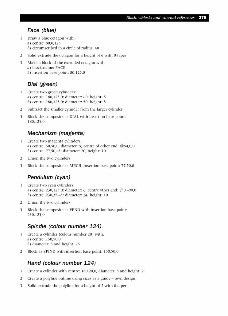
Face (blue)1 Draw a blue octagon with:
a) centre: 80,0,125b) circumscribed in a circle of radius: 40
2 Solid extrude the octagon for a height of 6 with 0 taper
3 Make a block of the extruded octagon with:a) block name: FACEb) insertion base point: 80,125,0
Dial (green)1 Create two green cylinders:
a) centre: 180,125,0; diameter: 60; height: 5b) centre: 180,125,0; diameter: 50; height: 5
2 Subtract the smaller cylinder from the larger cylinder
3 Block the composite as DIAL with insertion base point:180,125,0
Mechanism (magenta)1 Create two magenta cylinders:
a) centre: 50,50,0; diameter: 5; centre of other end: @54,0,0b) centre: 77,50,–5; diameter: 20; height: 10
2 Union the two cylinders
3 Block the composite as MECH, insertion base point: 77,50,0
Pendulum (cyan)1 Create two cyan cylinders:
a) centre: 230,125,0; diameter: 6; centre other end: @0,–90,0b) centre: 230,35,–5; diameter: 24; height: 10
2 Union the two cylinders
3 Block the composite as PEND with insertion base point:230,125,0
Spindle (colour number 124)1 Create a cylinder (colour number 20) with:
a) centre: 150,50,0b) diameter: 5 and height: 25
2 Block as SPIND with insertion base point: 150,50,0
Hand (colour number 124)1 Create a cylinder with centre: 180,20,0, diameter: 5 and height: 2
2 Create a polyline outline using sizes as a guide – own design
3 Solid extrude the polyline for a height of 2 with 0 taper
Block, wblocks and external references 279
modelling with AutoCAD.qxd 17/06/2002 15:42 Page 279

4 Subtract the cylinder from the extrusion
5 Block as HAND with insertion base point: 120,20,0
Inserting the blocks1 Still with UCS FRONT, layer MODEL and lower left viewport
2 Zoom centre about 0,75,0 at 200 magnification – all viewports
3 At the command line enter -INSERT <R> and:prompt Enter block name and enter: BODYprompt Specify insertion point and enter: 0,0,0prompt Enter X scale factor and enter: 1prompt Enter Y scale factor and enter: 1prompt Specify rotation angle and enter: 0
4 Insert the other blocks using the following information:name insertion pt scale rotFACE 0,125,0 X=Y=1 0DIAL 0,125,6 X=Y=1 0MECH 0,125,–10 X=Y=1 0PEND 0,125,–10 X=Y=1 0SPIND 0,125,–5 X=Y=1 0HAND 0,125,15 X=Y=1 0HAND 0,125,18 X=Y=0.75 –150
5 Shade the 3D viewport (Gouraud) the use the 3D orbit command. The result is veryimpressive
6 DO NOT union the inserted blocks but save as MODR2002\CLOCK for the renderingexercises.
Tasks1 Union the eight inserted blocks – explode needed? The model will be displayed with the
block inserted colours. Why is this different from the desk tidy example when the unioncommand resulted in the model being displayed in one colour? Think layers!
2 In the lower right viewport extract a profile of the model to display hidden detail andremember:a) hidden linetype must be loaded and set to the pH layerb) currently freeze layer MODEL in the viewportc) optimise the LTSCALE variable
3 In the top left viewport extract a vertical section through the model and remember:a) use the layer SECT with the required section planeb) add hatching to the region – UCS is importantc) currently freeze layer MODEL in this viewportd) currently freeze layer SECT in other viewports
4 Add an additional viewport to display the assembled model from below
5 The final layout should be as Fig. 42.4 and can be saved.
280 Modelling with AutoCAD 2002
modelling with AutoCAD.qxd 17/06/2002 15:42 Page 280

External references with solid modelsTo demonstrate how solid models can be used as wblocks and external references, arelatively simple layout will be created to represent a workshop, the machines being largemachining centres. Solid model composite will be used for these machining centres.
1 Open your A3SOL template file with MVLAY1 as normal
2 Restore the WCS with the command line entry UCS <R> then W <R>
3 Create the following primitives:box wedge wedge
corner: 0,0,0 100,0,70 100,80,70length: 100 –50 –50width: 80 15 –25height: 70 –50 –50colour: red blue green
4 Create a cylinder, centre at 20,0,70 and radius 20 with centre of other end at @0,80,0.This cylinder is to be magenta
5 Union the box and cylinder and subtract the two wedges from the composite. This modelrepresents the machining centre.
Block, wblocks and external references 281
Figure 42.4 Assembled wall clock with profile and section extraction..
modelling with AutoCAD.qxd 17/06/2002 15:42 Page 281

6 At the command line enter WBLOCK <R> and:prompt Write Block dialogue boxrespond 1. Source: objects
2. Base point with X: 0, Y: 0, Z: 03. Objects: pick Select objects and:
prompt Select objectsrespond pick the composite then right-clickprompt Write Block dialogue boxrespond 1. File name: MACH1
2. Location: c:\MODR2002 or named your folder3. Insert units: Millimeters4. pick OK
prompt Write block preview displayed at top left of screen
7 Erase the composite then create another box and cylinder with:a) box: corner at 0,–20,0 with cube option of length 40b) cylinder: centre at 40,0,20, radius 15 with centre of other end at @40,0
8 Change the colour of the box and cylinder to colour number 24 then union the twoprimitives. This model represents the robot feeder for the machining centres
9 Make a second wblock with:a) source: objectsb) base point: X 0, Y 0, Z 0c) objects: select objects, pick composite, right-clickd) file name: MACH2e) location: C:\MODR2002 or named your folderf) insert units: millimetersg) pick OK
10 Close the A3SOL file (no save) then re-open it again
11 Restore the WCS (UCS-W) then zoom centre about 0,100,50 at 300 magnification in allviewports
12 With the 3D viewport active, menu bar with Insert-External Reference and:prompt Select Reference File dialogue boxrespond 1. scroll and pick C:\MODR2002 or named your folder
2. scroll and pick MACH13. pick Open
prompt External Reference dialogue boxwith Name: MACH1respond 1. ensure all on-screen prompts active (tick)
2. reference type: Attachment3. pick OK
prompt Specify insertion point and enter: –200,–40,0 <R>prompt Enter X scale factor and enter: 1 <R>prompt Enter Y scale factor and enter: 1 <R>prompt Specify rotation angle and enter: 0 <R>
13 Polar array the insertion external reference about the point 0,0 for four items withrotation, the angle to fill being –180
282 Modelling with AutoCAD 2002
modelling with AutoCAD.qxd 17/06/2002 15:42 Page 282
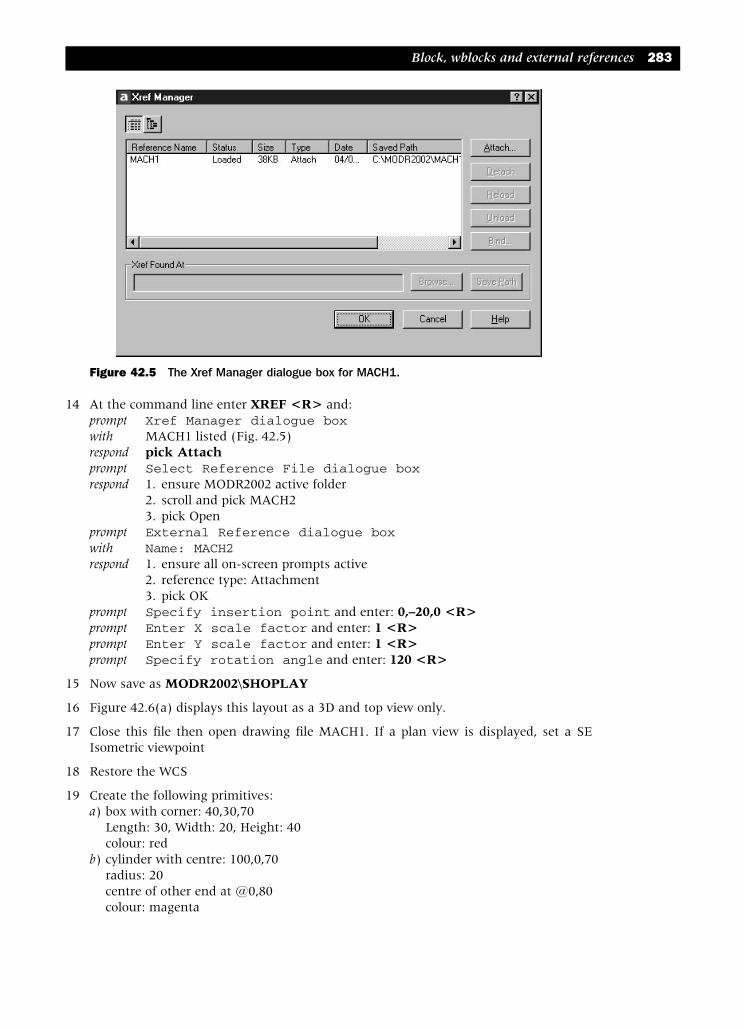
14 At the command line enter XREF <R> and:prompt Xref Manager dialogue boxwith MACH1 listed (Fig. 42.5)respond pick Attachprompt Select Reference File dialogue boxrespond 1. ensure MODR2002 active folder
2. scroll and pick MACH23. pick Open
prompt External Reference dialogue boxwith Name: MACH2respond 1. ensure all on-screen prompts active
2. reference type: Attachment3. pick OK
prompt Specify insertion point and enter: 0,–20,0 <R>prompt Enter X scale factor and enter: 1 <R>prompt Enter Y scale factor and enter: 1 <R>prompt Specify rotation angle and enter: 120 <R>
15 Now save as MODR2002\SHOPLAY
16 Figure 42.6(a) displays this layout as a 3D and top view only.
17 Close this file then open drawing file MACH1. If a plan view is displayed, set a SEIsometric viewpoint
18 Restore the WCS
19 Create the following primitives:a) box with corner: 40,30,70
Length: 30, Width: 20, Height: 40colour: red
b) cylinder with centre: 100,0,70radius: 20centre of other end at @0,80colour: magenta
Block, wblocks and external references 283
Figure 42.5 The Xref Manager dialogue box for MACH1.
modelling with AutoCAD.qxd 17/06/2002 15:42 Page 283
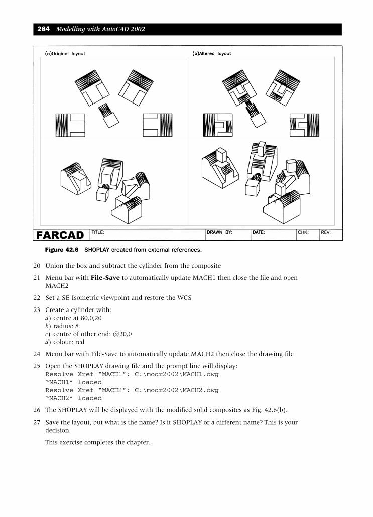
20 Union the box and subtract the cylinder from the composite
21 Menu bar with File-Save to automatically update MACH1 then close the file and openMACH2
22 Set a SE Isometric viewpoint and restore the WCS
23 Create a cylinder with:a) centre at 80,0,20b) radius: 8c) centre of other end: @20,0d) colour: red
24 Menu bar with File-Save to automatically update MACH2 then close the drawing file
25 Open the SHOPLAY drawing file and the prompt line will display:Resolve Xref “MACH1”: C:\modr2002\MACH1.dwg“MACH1” loadedResolve Xref “MACH2”: C:\modr2002\MACH2.dwg“MACH2” loaded
26 The SHOPLAY will be displayed with the modified solid composites as Fig. 42.6(b).
27 Save the layout, but what is the name? Is it SHOPLAY or a different name? This is yourdecision.
This exercise completes the chapter.
284 Modelling with AutoCAD 2002
Figure 42.6 SHOPLAY created from external references.
modelling with AutoCAD.qxd 17/06/2002 15:42 Page 284

SummaryBlocks, wblocks and eternal references can be used with solid modelling as with anyother type of drawing layout.
AssignmentIn activity 23, the garden block of MACFARAMUS was created. This object was used formany building projects in various parts of the city of CADOPOLIS. Part of a garden projectwas unearthed which contained a wall, gate and path. The original garden block has tobe saved as a block (no pun intended) and used to create the wall, gate and path.
ACTIVITY 24: Using the garden block of MACFARAMUS
1 Open the activity 22 drawing and create a block of the garden block with:a) name: GRADBLb) base point: pick the suit – suggest 0,0c) select the objectd) ensure insert units are millimetres
2 Wall: with UCS RIGHTa) insert the GRADBL at a suitable pointb) the scales are full sizec) create a suitable wall layout
3 Gate: with UCS RIGHTa) insert the GARDBL at the correct point relative to the wallb) scales are X: 2, Y: 3, Z: 0.5
4 Path: with UCS BASEa) insert the GRADBL at the correct point relative to the gateb) scales are X: 2, Y: 1, Z: 0.25
5 Optimise your layout and save
Block, wblocks and external references 285
modelling with AutoCAD.qxd 17/06/2002 15:42 Page 285
The setup commandsThe setup commands (Drawing, View and Profile) allow drawing layouts to be createdby the user. As the profile command has been discussed in a previous chapter, we willonly consider the View and Drawing commands in this chapter. These two commandscan be summarised as:
View: creates floating viewports using orthographic projection to lay-out multi andsectional views of 3D solid models.
Drawing: generates profiles and sections in viewports which have been created withthe setup VIEW command.
Basically the two commands allow the user to create multiple viewport configurationswhich will display top, front, end and auxiliary views as well as extracting profile andsections of the model. In other words the two commands will create the same type oflayout that has been achieved with our A3SOL template file, the 3D viewpoint commandand with the SECTION and PROFILE commands.
We will demonstrate the two commands using previously created models.
Example 1 – the backing plate1 Open the drawing file MODR2002\BACKPLT from chapter 32 and:
a) MVLAY1 tab activeb) restore UCS BASE with layer MODEL currentc) in paper space erase the viewports except the 3D viewd) scale the 3D viewport about the lower left corner by 0.3e) in paper space ensure the paper space icon is relative to World by command line entry
UCS <R> then W <R>f) in model space, zoom extents
2 Refer to Fig. 43.1
Chapter 43
modelling with AutoCAD.qxd 17/06/2002 15:42 Page 286
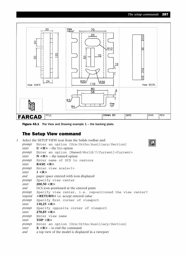
The Setup View command1 Select the SETUP VIEW icon from the Solids toolbar and:
prompt Enter an option [Ucs/Ortho/Auxiliary/Section]enter U <R> – the Ucs optionprompt Enter an option [Named/World/?/Current]<Current>enter N <R> – the named optionprompt Enter name of UCS to restoreenter BASE <R>prompt Enter view scale<1>enter 1 <R>and paper space entered with icon displayedprompt Specify view centerenter 200,50 <R>and UCS icon positioned at the entered pointprompt Specify view center, i.e. repositioned the view center?respond <RETURN> i.e. accept entered valueprompt Specify first corner of viewportenter 130,25 <R>prompt Specify opposite corner of viewportenter 270,85 <R>prompt Enter view nameenter TOP <R>prompt Enter an option [Ucs/Ortho/Auxiliary/Section]enter X <R> – to end the commandand a top view of the model is displayed in a viewport
The setup commands 287
Figure 43.1 The View and Drawing example 1 – the backing plate.
modelling with AutoCAD.qxd 17/06/2002 15:42 Page 287

2 Menu bar with Draw-Solids-Setup-View and:prompt Enter an option [Ucs/Ortho/Auxiliary/Section]enter O <R> – the ortho optionprompt Specify side of viewport to projectrespond pick bottom horizontal line of the new viewport and note the midpoint snap
effectprompt Specify view center and enter: 200,170 <R>prompt Specify view center and <RETURN>prompt Specify first corner of viewport and enter: 130,85 <R>prompt Specify opposite corner of viewport and enter: 270,245 <R>prompt Enter view name and enter: FRONT <R>prompt Enter an option [Ucs/Ortho/Auxiliary/Section] and enter: X <R>
3 A front view of the model is displayed in a viewport
4 At the command line enter SOLVIEW <R> and:prompt Enter an option [Ucs/Ortho/Auxiliary/Section] and enter: O <R>prompt Specify side of viewport to projectrespond pick right vertical line of the new (front) viewportprompt Specify view center and enter: 80,165 <R>prompt Specify view center and <RETURN>prompt Specify first corner of viewport and enter: 130,85 <R>prompt Specify opposite corner of viewport and enter: 25,245 <R>prompt Enter view name and enter: SIDER <R>prompt Enter an option [Ucs/Ortho/Auxiliary/Section] and enter: X <R>
5 A right view of the model is displayed
6 Activate the setup View command and:prompt Enter an option [Ucs/Ortho/Auxiliary/Section]enter S <R> – the section optionprompt Specify first point of cutting planerespond 1. pick the new ‘front’ viewport
2. enter 0,0,0 <R>prompt Specify second point of cutting planeenter 0,120 <R>and a dashed ‘section’ line is displayedprompt Specify side to view fromrespond pick a point to left of section lineprompt Enter view scale and enter: 1 <R>prompt Specify view center and enter: 320,165 <R>prompt Specify view center and <RETURN>prompt Specify first corner of viewport and enter: 270,85 <R>prompt Specify opposite corner of viewport and enter: 370,245 <R>prompt Enter view name and enter: SECTL <R>prompt Enter an option [Ucs/Ortho/Auxiliary/Section]enter X <R>
7 A left view of the model is displayed
8 Note:a) In the example I have given coordinates for the view centre point, the viewport
corners, the section line etc. It is usual to ‘pick these points’ on the screen rather thanenter coordinates. The only reason for the coordinate entry was that this was our firstexample and it should help the user understand the responses to the various prompts
b) The view names can be entered as V1, V2, etc. or as TOP, FRONT. This is dependenton the user. Just ensure that you know what view has been allocated to the name.
288 Modelling with AutoCAD 2002
modelling with AutoCAD.qxd 17/06/2002 15:42 Page 288

Investigating the layers1 Menu bar with Format-Layer and note the new layer names:
a) FRONT-DIM, FRONT-HID, FRONT-VISb) SECTL-DIM, SECTL-HAT, SECTL-HID, SECTL-VISc) SIDER-DIM, SIDER-HID, SECTR-VISd) TOP-DIM, TOP-HID, TOP-VISe) VPORTS
2 Each new viewport has a dimension, hidden and visible layer and the section viewporthas a hatch layer
3 In model space make the TOP viewport active and activate the Layer Properties Managerdialogue box. The three FRONT, four SECTL and three SIDER layers are all frozen in thiscurrent viewport.
4 Using the Layer Properties Manger dialogue box, load the HIDDEN linetype and set thefour -HID layers to this linetype. The reason for this will become obvious.
5 The new layers are automatically created with the SETUP VIEW command and areviewport specific as follows: a) -DIM: for dimensionsb) -HID: for hidden detail c) -VIS: for visible linesd) -HAT: for hatching detail if the section option has been used
The Setup Draw command1 In model space with any viewport active, set the following system variables from the
command line:command line enterHPNAME ANSI31HPANG 0HPSCALE 1
2 Select the SETUP DRAW icon from the Solids toolbar and:and paper space enteredprompt Select viewports to drawthen Select objectsrespond pick the four new viewports borders then right-click
3 The four new viewports will display the model:a) with hidden line removal: top, front, rightb) as a section: left – with no hidden detailc) you should now understand why the HIDDEN linetype was loaded and set to certain
layers, and why the three HP system variables were set
4 Optimise the LTSCALE system variable for the hidden line detail
5 Note:a) The three command line entries of HPNAME, HPANG and HPSCALE have set the
hatch pattern name, angle and scale. This could have been achieved after the hatchingwas added to the section view with the Modify-Hatch command.
b) Note the model space icon in each viewport has the same orientation. This is becausewhen new viewports are created, the UCSVP system variable defaults to 1, i.e. theUCS icon will have the same configuration in each new viewport. We will leave it asit is.
The setup commands 289
modelling with AutoCAD.qxd 17/06/2002 15:42 Page 289

6 Task: Add dimensions to the new viewports remembering:a) the -DIM layers are viewport specific but need to be current in the appropriate
viewportb) is a named UCS required for this?c) Fig. 43.1 displays the complete layout with dimensions
These dimensions have been added without altering the UCS orientation. They arealso viewport specific dimensions and not paper space dimensions. Thus this isanother method of adding dimensions to a drawing layout
d) save the model with your own entered file name
Example 2 – the slip block1 Open model MODR2002\SLIPBL from chapter 37 and:
a) in paper space erase three viewports to leave the 3D viewb) in model space restore UCS BASE and layer MODELc) refer to Fig. 43.2
2 Use the Setup View command with:a) options: Ub) UCS options: N then BASEc) view scale: 0.5d) view center: 190,90 then <RETURN>e) first corner of viewport: 130,50f) opposite corner of viewport: 250,130g) view name: V1h) options: X
290 Modelling with AutoCAD 2002
Figure 43.2 The setup View and Drawing example 2 – the slip block.
modelling with AutoCAD.qxd 17/06/2002 15:42 Page 290

3 In paper space erase the original 3D view then return to model space
4 Use the SOLVIEW command with:a) options: Ub) UCS options: N then FRONTc) view scale: 0.5d) view center: 190,170 then <RETURN>e) first corner of viewport: 250,130f) opposite corner of viewport: 130,210g) view name: V2h) options: X
5 In model space make the new viewport active – should be
6 With the SOLVIEW command use the following:a) options: S – sectionb) first point of cutting plane: 50,0c) second point of cutting plane: 50,100d) side to view from: pick to right of the section linee) view scale: 0.5f) view centre: 0,100 (note icon effect) then <RETURN>g) first corner of viewport: 130,210h) opposite corner of viewport: 10,130i) view name: V3j) options: X
7 Activate the Setup View command and:prompt Enter an option [Ucs/Ortho/Auxiliary/Section]enter A <R> – the auxiliary optionprompt Specify first point of inclined planerespond make first new viewport activeand ENDpoint icon and pick pt1prompt Specify second point of inclined planeenter @100<–60 <R>prompt Side to view fromrespond pick ‘below’ the inclined planeprompt View centreenter 0,175 <R> then <RETURN>prompt Specify first corner of viewport and enter: 250,100 <R>prompt Specify opposite corner of viewport and enter: 390,240 <R>prompt View name and enter: V4 <R>prompt Enter an option [Ucs/Ortho/Auxiliary/Section] and enter: X <R>
8 Select the Setup Drawing icon and pick the four new viewport borders and the displaywill be:a) as a section: the left viewportb) with hidden line removal: the other three viewports after the HIDDEN linetype has been
loaded and set to the -HID layers and the LTSCALE system variable has been optimised
9 Note the hatch effect is the ANGLE hatch pattern. This is the default setting
10 To alter the hatch pattern, enter model space and make the left(section)viewport active.Restore UCS RIGHT
The setup commands 291
modelling with AutoCAD.qxd 17/06/2002 15:42 Page 291

11 Menu bar with Modify-Object-Hatch and:prompt Select associative hatch objectrespond pick the hatchingprompt Hatch Edit dialogue boxrespond 1. Type: User-defined
2. Angle: 453. Spacing: 44. pick OK
12 The model layout is now as Fig. 43.2 and can be saved
13 Note: the view centre entry with the section and auxiliary options is perpendicular tothe paper space icon. This icon is orientated relative to the:a) section plane b) auxiliary inclined plane
Example 3 – the pipe and flange model1 Open the drawing file MODR2002\FLPIP created in chapter 33 and:
a) paper space to erase the viewports leaving the 3D viewb) model space with UCS BASE and layer MODEL currentc) load the linetype HIDDENd) set the LTSCALE variable value to a suitable valuee) set the following hatch variables:
HPNAME: ANSI32; HPANG: 0; HPSCALE: 1f) paper space scale the 3D viewport by 0.5 and move to the top left of the drawing sheetg) model space and zoom the model in the 3D viewport to a suitable sizeh) refer to Fig. 43.3 for the viewport layouts
292 Modelling with AutoCAD 2002
Figure 43.3 Setup view and drawing example 3 – the flange/pipe model.
modelling with AutoCAD.qxd 17/06/2002 15:43 Page 292

2 Activate the setup View command and:a) UCS option with UCS BASEb) view scale: 0.25c) view centre: 200,200d) position viewport: pick to suit yourselfe) name: MYVIEW1f) options: X
3 Repeat the setup View command:prompt Enter an option [Ucs/Ortho/Auxiliary/Section]enter O <R> – the ortho optionprompt Specify side of viewport to projectrespond pick lower horizontal line of viewport prompt Specify view centerenter 200,100 <R>prompt Specify view centreand pick to suit yourselfprompt Specify corners of viewportrespond pick to suit your layoutprompt Enter view name and enter: MYVIEW2 <R>prompt Enter an option and continue with next part of exercise
4 Setup view command still active with options:a) select the Ortho optionb) pick right vertical line of second viewportc) view center: pick a point to right to suitd) viewport corners: pick points to suite) view name: MYVIEW3f) optionsg) select the Auxiliary optionh) Inclined plane points: pick to suit – see Fig. 43.3i) Side to view from: pick ‘below’ the inclined linej) view center: pick a point to suitk) viewport corners: position to suitl) view name: MYVIEW4m) optionsn) select the section optiono) cutting plane points: pick points as indicated in Fig. 43.3p) side to view from: pick to right of the section lineq) view scale: 0.25r) view center: pick to suits) viewport corners: pick to suit the layoutt) name: MYVIEW5u) options: X to end command
5 Linetype HIDDEN and three HP variables set?
6 Activate the Setup Drawing command and pick the five viewports to display the layoutwith hidden line removal and section detail as Fig. 43.3
7 Freeze layer VPORTS if required
8 QuestionIn our three setup examples the type of layout has not been mentioned, i.e. first or thirdangle. I am sure that you are aware of the projections obtained, the first two examplesbeing in first angle, and the third example being in third angle. This is the ‘power’ ofthe setup commands. First and third angle detail layouts can be obtained for models bysimply picking the relevant view centre points
9 Save the exercise as it is now complete.
The setup commands 293
modelling with AutoCAD.qxd 17/06/2002 15:43 Page 293

Summary1 The set View and Drawing commands allow the user to layout multi-view drawings
without the need to create viewports and set viewpoints
2 Both commands can be activated:a) by selecting the icon from the Solids toolbarb) from the menu bar with Draw-Solids-Setupc) from the command line with SOLVIEW and SOLDRAW
3 The setup View command has options which allow views to be created:a) relative to a named UCSb) as an orthographic view relative to a selected viewportc) as an auxiliary view relative to an inclined planed) as a section view relative to a cutting plane
4 When used, the View command creates viewport specific layers, these being relative tothe viewport handle number with the following names:-VIS for visible lines-HID for hidden lines-DIM for dimensions-HAT for hatching but only if the section option is used
5 The View command requires the user to:a) enter the view scaleb) position the viewport centre pointc) position the actual viewport corners
6 With the Ortho option, both First and Third angle projections can be obtained dependenton which side the new viewport is to be placed
7 The section option requires that the system variables HPNAME, HPANG and HPSCALEare set. It is usual to use the ANSI31 hatch pattern name, but this is not essential.AutoCAD defaults the ANGLE hatch pattern
8 The Drawing command will display models which have been created with the Viewcommand:a) with visible and hidden detailb) as a section if the section option has been used
9 It is recommended that the linetype HIDDEN be loaded before the Drawing commandis used.
10 The hidden linetype appearance is controlled by the LTSCALE system variable.
11 The user now has two different methods for creating multi-view layouts of solid models:a) using the A3SOL template file idea which sets the viewports and viewpoints prior to
creating the model. Profiles can then be extracted to display hidden detailb) using the VIEW and DRAWING commands with a solid composite to layout the
drawing in First or Third angle projection with sections and auxiliary views asrequired.
c) it is now the user’s preference as to which method is used
12 Dimensions can now be added to models:a) using viewport specific layersb) using paper space dimensioningc) using the setup commands
294 Modelling with AutoCAD 2002
modelling with AutoCAD.qxd 17/06/2002 15:43 Page 294

The final compositeWe have now covered virtually every concept of solid modelling within the AutoCADdraughting package. The next chapter will introduce the user to rendering, but beforethat we will make a final solid model using the various techniques that have beendiscussed. The model is quite involved, so try not to miss out any of the steps, especiallythose which set a new UCS position.
The three examples selected to demonstrate the View and Drawing commands have usedpreviously created models. This example will create a new model ‘from scratch’.
1 Open your A3SOL template/drawing file with layer MODEL, UCS BASE and make themodel tab active. We will use this tab to create the model and then set up our drawinglayout with the MVLAY1 tab
2 Set ISOLINES to 6 and refer to Fig. 44.1
3 The new model will be created from five primitives, each requiring a new UCS position.
Chapter 44
Figure 44.1 Construction of the computer link model.
modelling with AutoCAD.qxd 17/06/2002 15:43 Page 295

Primitive 1: the base1 Rotate the UCS about the X axis by 90 and save as PRIM1
2 Draw a polyline:a) start point: 0,50 b) next point: @60,0 c) next point: @0,–40d) arc option with endpoint: @–10,–10 e) line option to: @–40,0 f) arc option with endpoint: @–10,10g) line option to: close
3 Zoom extents then zoom to a scale of 3
4 Solid extrude the polyline for a height of 3 with 0 taper
5 Create two cylinders:a) centre: 30,25,0; radius: 6; height: 3b) centre: 30,40,0; radius: 3; height: 3
6 Polar array the smaller cylinder about the point 30,25 for 3 items with full circle rotation
7 Subtract the four cylinders from the extruded polyline – fig(a)
Primitive 2: wedge on top of first primitive1 UCS PRIM1 current
2 Set a new 3 point UCS position with:a) origin: 0,50,0b) x-axis: 60,50,0c) y-axis: 0,50,3d) save as: PRIM2
3 Create a wedge with:a) corner: 0,0,0b) length: 60; width: –3; height: –30
4 Rotate 3D this wedge:a) about the X axisb) with 0,0,0 as a point on the axisc) for 90 degrees
5 Union the wedge and the extruded polyline – fig(b)
Primitive 3: box on top of wedge1 UCS PRIM2 current
2 Set a new 3 point UCS position with:a) origin: 60,0,0b) x-axis: 0,30,0c) y-axis: 60,0,–3d) save as: PRIM3
3 Create a solid box with a) corner: 0,0,0b) length: 67.08; width: 30; height: –3. Why 67.08?
296 Modelling with AutoCAD 2002
modelling with AutoCAD.qxd 17/06/2002 15:43 Page 296

4 Create a cylinder with: a) centre: 10,10,0 and:b) radius: 3; height: –3
5 Rectangular array the cylinder:a) for 2 rows and 3 columnsb) row offset: 10; column offset: 15
6 a) subtract the six cylinders from the boxb) union the box and the composite – fig(c)
Primitive 4: curved extension on top of box1 Pan the model to lower part of screen
2 UCS PRIM3 current
3 Set a new 3 point UCS position with:a) origin: 0,30,–3b) x-axis: 67.08,30,–3c) y-axis: 0,30,0d) save as: PRIM4
4 Zoom in on the ‘free edge’ of the box
5 Draw two line segments with: start point: 0,0 next point: @0,–15; next point: @50,0
6 Draw a polyline about the ‘top rim’ of the box using the ENDpoint snap and the closeoption
7 With the solid revolve command:a) objects: enter L <R><R> – to select the polylineb) options: enter O <R> – object optionc) object: pick the left end of long construction lined) angle: enter 120
8 Erase the two line segments
9 Zoom previous to restore original view
10 Union the revolved component and the composite – fig(d)
Primitive 5: final curved component1 UCS PRIM4 current
2 Set a new 3 point UCS position with:a) origin: 67.08,–22.5,–12.99b) x-axis: 0,–22.5,–12.99c) y-axis: 67.08,–24,–15.59d) save as: PRIM5e) can you work out the three sets of coordinates?
3 Zoom-in on the ‘free end’ of the curved component
4 Draw a polyline about the free end of the curved component using the ENDpoint snapand the close option
The final composite 297
modelling with AutoCAD.qxd 17/06/2002 15:43 Page 297

5 With the Solid revolve command:a) objects: enter L <R><R> – to select the polylineb) options: enter Y <R> – the Y axisc) angle: enter –30
6 Create a cylinder with:a) centre: 45,0,15b) radius: 5c) centre of other end: @0,10,0
7 Subtract the cylinder from the revolved component, then union the revolvedcomponent with the cylinder – fig(e)
8 Zoom previous to restore the original view
9 The model is now complete, so:a) Gouraud shade and 3D orbit – impressive?b) restore 2D wireframe representation at the original viewpoint
10 a) restore UCS BASEb) save as MODR2002\COMPLINK
Laying out the viewportsThis part of the exercise will use the MVLAY1 tab with all options of setup Viewcommand.
1 Pick the MVLAY1 tab name
2 In paper space:a) erase three viewports but leave the 3D viewportb) stretch (crossing option) the two vertical edges of the 3D viewport by @50,0 (left side)
and @–50,0 (right side)c) move the 3D viewport as far left as possibled) in model space, UCS BASE, layer Model current and zoom the model to suit
3 a) load linetype HIDDENb) set the following variables:
HPNAME: ANSI31; HPANG: 0; HPSCALE: 0.5c) set the LTSCALE value to suit which may change after the layout has been created
4 Activate the setup View command with:a) UCS option with BASEb) view scale: 1c) view center: 175,75d) viewport corners: pick to suite) view name: TOPf) options: X
5 Using the SOLVIEW command:a) UCS option with PRIM1 as the named UCSb) view scale: 1c) view center: 175,200d) viewport corners: pick to suite) view name: FRONTf) exit command or continue with command
298 Modelling with AutoCAD 2002
modelling with AutoCAD.qxd 17/06/2002 15:43 Page 298

6 SOLVIEW command with:a) Ortho optionb) side: pick right vertical side of the second viewportc) view center: 50,200d) viewport corners: pick to suite) view name: RIGHTf) exit command or continue with command
7 With the setup View command:a) activate the Section optionb) pick any point in the second viewportc) cutting plane points: 30,0 and 30,120d) side to view from: pick a point to left of section linee) view scale: 1f) view center: 0,–110g) viewport corners: pick to suith) view name: SECTIONi) exit or continue with command
8 The final SOLVIEW command is with:a) the Auxiliary optionb) first point of inclined plane and with the first viewport active, pick ENDpoint of pt1
(see Fig. 44.2)c) second point of inclined plane: PERP to line 23d) side to view from: pick to left of inclined linee) view center: 0,200f) viewport corners: pick to suitg) view name: AUXILIARYh) end the command
The final composite 299
Figure 44.2 Computer link detail drawing using the setup commands.
modelling with AutoCAD.qxd 17/06/2002 15:43 Page 299

9 Using the setup Drawing command, pick the five viewports to display hidden detail anda section view – linetype HIDDEN loaded?
10 Now optimise the LTSCALE system variable
11 Tasksa) Interrogate the model in the 3D viewport:
Area: 20196.01Mass: 26758.64
b) Using the viewport specific -DIM layers, add the dimensions displayed in Fig. 44.2.The UCS in the new created viewports should be ‘set’ to allow this as the UCSVPsystem variable always defaults to 1 when a new viewport is created. Note that a paperspace zoom of the viewport being dimensioned will assist with the dimensions.
c) Freeze the VP and VPORTS layersd) In paper space, optimise your drawing with suitable texte) Save the completed exercise – worth the effort?
AssignmentTo give some additional practice with the View and Drawing commands I have includedanother new model to be created.
Activity 25 – dispenser of MACFARAMUS
One of the discoveries in the city of CADOPOLIS was a container which was thought tobe a dispenser belonging to MACFARAMUS. It is this container which has to be createdas a solid model and then displayed with the setup commands.
1 Use your template file with the Model tab active and when the model is complete usethe MVLAY1 tab as the chapter example
2 Make two new layers BODY blue and TOP green
3 With UCS FRONT, draw the two shapes using the reference sizes in Fig. 44.3. Use thestart points given. Draw as lines/arcs then use the join option of the modify polylinecommand to convert the segments into single polylines.
300 Modelling with AutoCAD 2002
Figure 44.3 Reference details for activity 25.
modelling with AutoCAD.qxd 17/06/2002 15:43 Page 300

4 Solid revolve the two polylines for a full circle
5 Create the holes in the top
6 Create a handle from a hexagon, the actual shape being at your discretion – I extrudeda hexagon along a polyline path
7 Use the VIEW and DRAWING commands to create a multi-view layout to display:a) top and front views with hidden detailb) two section views through the planes indicatedc) an auxiliary view through an inclined plane at 45 degrees d) a 3D viewe) I used a view scale of 0.6
8 This activity should highlight a problem when the setup commands are used with amodel containing more than one part. The dispenser has a top and a body, but whenthe section option is used, the same hatching is added to both parts. How would differenthatching be added to the two parts?
The final composite 301
modelling with AutoCAD.qxd 17/06/2002 15:43 Page 301
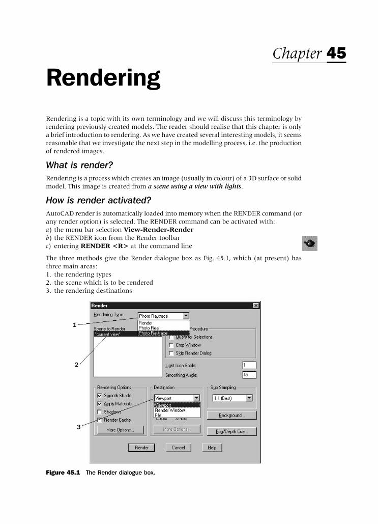
RenderingRendering is a topic with its own terminology and we will discuss this terminology byrendering previously created models. The reader should realise that this chapter is onlya brief introduction to rendering. As we have created several interesting models, it seemsreasonable that we investigate the next step in the modelling process, i.e. the productionof rendered images.
What is render?Rendering is a process which creates an image (usually in colour) of a 3D surface or solidmodel. This image is created from a scene using a view with lights.
How is render activated?AutoCAD render is automatically loaded into memory when the RENDER command (orany render option) is selected. The RENDER command can be activated with:a) the menu bar selection View-Render-Renderb) the RENDER icon from the Render toolbarc) entering RENDER <R> at the command line
The three methods give the Render dialogue box as Fig. 45.1, which (at present) hasthree main areas:1. the rendering types2. the scene which is to be rendered3. the rendering destinations
Chapter 45
Figure 45.1 The Render dialogue box.
1
3
2
modelling with AutoCAD.qxd 17/06/2002 15:43 Page 302

Rendering typesAutoCAD has three ‘types’ of rendering, these being:1. Render: the basic AutoCAD render option which allows models to be rendered without
the need for scenes, lights or materials. This is the default ‘setting’ 2. Photo Real: is a photo-realistic renderer which can display bitmapped and transparent
materials. Volumetric and mapped shadows can also be generated.3. Photo Raytrace: is a photo-realistic raytrace renderer which can generate reflections,
refraction and precise shadows.
Rendering destinationThe rendered image of the model can be:1. displayed in the current viewport of a multi-screen layout2. displayed in the render window3. saved to a file for future recall
Scene to renderAllows the user to select a named scene of the model to render. The user can ‘make’ severalscenes using different views of the model with various lights and materials added.AutoCAD provides a ‘default’ scene for rendering purposes. This default scene uses a distantlight which cannot be modified by the user. At all times it should be remembered that:
*** A scene is a view with lights added ***
The AutoCAD lightsAdding lights to a model layout immediately improves the render appearance and lights canbe used to illuminate a complete model or to highlight specific parts of the layout. AutoCAD2002 has four ‘types’ of light available, these being ambient, distant, point and spot.
Ambient light1 Provides a constant illumination to all surfaces of a model.
2 It is always ‘there’ and does not originate from any particular source.
3 The user has control of the intensity of the ambient light
4 Generally the ambient light intensity should be a low value or the model will be displayed‘too bright’
5 The default ambient intensity value is 0.3
6 Ambient light on its own does not produce good rendered images.
Distant light1 Gives a parallel beam in a particular direction
2 The user specifies the target point and the light source location
3 Think of a torch shining at an object
4 Distant light rays extend to infinity on either side of the light source
5 The distant light intensity is not affected by the distance of the source from the target
6 It is recommended that distant lights are positioned at the extents of the drawing
7 Distant lights are used to give a ‘uniform lighting’ facility
8 A single distant light simulates the sun
Rendering 303
modelling with AutoCAD.qxd 17/06/2002 15:43 Page 303

Point light1 A point light emits light in all directions from its position
2 The user specifies the point light location
3 Think of a light bulb
4 The intensity of a point light is affected by the distance from the model
5 Point lights are used for general lighting effects
6 Point lights are used with spot lights for lighting effects
Spot light1 Gives a directional cone of light
2 The user specifies the direction of the light and the size of the cone
3 The intensity of a spot light diminishes with the distance from the model
4 Spot lights have ‘hot-spots’ and ‘fall-off angles’ that determine how the lightdiminishes at the edge of the cone
5 Spot lights can be used to highlight specific features on a model.
Point lights, distant lights and spot lights are represented in a drawing with symbols,the light name being displayed within the light symbol – Fig. 45.2
Note1 Lights are essential for rendering and their position in relation to the model is very
important. AutoCAD will position a light in the centre of the active viewport, irrespectiveof the model position. The user must know exactly where the light is to be positionrelative to the model. This can be achieved using coordinates and object snaps. It is alsoimportant for the user to know the basic sizes of the model and its where the model issituated on the drawing screen. This is one of the main reasons that I use the 0,0,0 originpoint when creating models.
2 The basic ‘order’ with rendering is:a) create the modelb) make a view for a particular model 3D viewpointc) position lights – with or without shadowsd) add materials to the model partse) make a scene from a view and lightsf) render with a type and to a destination
304 Modelling with AutoCAD 2002
Figure 45.2 Light symbols with ‘names’ added.
modelling with AutoCAD.qxd 17/06/2002 15:43 Page 304

Models to be renderedTwo previously created solid models will be used be demonstrate how lights, scenes,materials, shadows, etc. can be added to a layout and produce a rendered coloured image.The models selected are the extruded backing plate and the wall clock.
Render example 1 – the solid model backing plateWhen rendering a model, the user will activate several dialogue boxes. It is not myintention to display these dialogue boxes (other than Render) in the exercise. Thenecessary steps to activate parts of these dialogue boxes will be given, and the user caninvestigate other ‘parts’ of these dialogue boxes at their leisure.
1 Open your saved drawing MODR2002\BACKPLT from chapter 32
2 Make the model tab active and set a SE Isometric viewpoint
3 a) Ensure UCS BASE and layer Model currentb) Ensure that the model is positioned with the mid-point of the front bottom edge at
the origin. It should be, but if it is not, move the model so that it is. This is importantfor positioning the lights
c) Display the Render toolbar
4 For maximum effect we want the lights to ‘cast shadows’ and we will create a base forthe model to stand on and a back wall, so from the menu bar select Draw-Solids-Boxand create two box primitives with:
box 1 box 2a) corner: –70,–20,0 –70,78,0b) length: 200 200c) width: 100 2d) height: –2 100e) colour: number 41 number 41
5 Union the two box primitives then zoom extents. The complete model layout should bedisplayed
6 The viewAs stated earlier, once the model has been created a view should be saved, and we willuse our existing screen layout for this, so at the command line enter VIEW <R> and:prompt View dialogue boxrespond 1. pick Named View tab
2. pick Newprompt New View dialogue boxrespond 1. View name: enter V1
2. Current display and Save UCS with view active3. UCS name: BASE4.pick OK
prompt View dialogue boxwith V1 listed with detailsrespond pick OK
7 Note that –VIEW <R> will allow command line entry
Rendering 305
modelling with AutoCAD.qxd 17/06/2002 15:43 Page 305

8 The lightsSelect the LIGHTS icon from the render toolbar and: prompt Lights dialogue boxrespond 1. set Ambient Light Intensity to 0.3
2. scroll at New and pick Point Light3. pick New
prompt New Point Light dialogue boxrespond 1. Light name: enter P1
2. Intensity: alter to 703. pick Modify
prompt Drawing screen returned with rubber band effect to lightposition which is at the ‘centre of the viewport’ i.e.the screen in this case
and Enter light location<current>enter 0,–50,100 <R> i.e. in front of the modelprompt New Point Light dialogue boxrespond 1. activate Shadows on – tick
2. pick Shadows Optionsprompt Shadows Options dialogue boxrespond 1. ensure Shadow Volumes/Ray Traced Shadows active
2. pick OKprompt New Point Light dialogue boxrespond pick OKprompt Lights dialogue box with P1 listedrespond 1. scroll at New and pick Distant Light
2. pick Newprompt New Distant Light dialogue boxrespond 1. Light name: enter D1
2. Intensity: alter to 0.93. pick Modify
prompt Drawing screen returned with rubber band effect to lightposition at centre of screen
and Enter light direction TOenter 50,0,30 <R>prompt Enter light direction FROMenter @20,–30,30 <R>prompt New Distant Light dialogue boxrespond 1. activate Shadows on
2. pick Shadows Optionsprompt Shadows Options dialogue boxrespond 1. ensure Shadow Volumes/Ray Traced Shadows active
2. pick OKprompt Distant Light dialogue boxrespond pick OK prompt Lights dialogue box with D1 and P1 listedrespond pick OK
9 The sceneMenu bar with View-Render-Scene and:prompt Scenes dialogue boxrespond pick Newprompt New Scenes dialogue boxrespond 1. enter Scene name: SC1
2. pick Views: V13. pick Lights: *ALL*4. pick OK
prompt Scenes dialogue box with SC1 listedrespond pick OK
306 Modelling with AutoCAD 2002
modelling with AutoCAD.qxd 17/06/2002 15:43 Page 306

10 The first renderAt the command line enter RENDER <R> and:prompt Render dialogue boxrespond 1. Rendering Type: scroll and pick Photo Real
2. Scene to Render: pick SC13. Destination: scroll and pick Render Window4. Rendering Options: ensure Smooth Shade, Apply Materials and Shadows
are active (tick)5. pick Render
prompt Render window will be displayed with a coloured image ofthe backing plate
and The rendered image should be reasonably impressive and the user shouldobserve:a) two shadow effectsb) a white backgroundc) the light effect on the model being ‘too bright’
respond pick AutoCAD from the Windows taskbar to return to the drawing screen
11 The user has now to decide whether the lights are in the correct position, is the intensityset correctly etc. We will leave the light settings as they are.
12 The backgroundWe now want to add a background to enhance the display and AutoCAD allows renderedimages to be displayed with four ‘types’ of background, these being:a) the default white backgroundb) a one coloured backgroundc) a gradient background of three coloursd) a ‘picture’ background of an already saved image
13 Select the BACKGROUND icon from the Render toolbar and: prompt Background dialogue boxrespond 1. Select Gradient
2. Accept the RGB colour settings3. Alter Horizon: 0.7; Height: 0.5; Rotation: –204. pick Preview then OK
14 Render scene SC1 with Photo Real to the Render Window and the model image will bedisplayed with the set gradient background
15 Return to the AutoCAD screen
16 Attaching a materialThe rendered image of the model is displayed with the colours of the primitives fromwhich it was created. AutoCAD has a library which allows the user to attach differentmaterials to surface and solid models, so select the Materials Library icon from theRender toolbar and:prompt Materials Library dialogue boxwith a) Materials in Current Drawing – Global
b) Current Library listrespond 1. scroll at Current Library list
2. pick WOOD-WHITE ASH3. scroll at Preview, pick Cube then pick Preview4. pick <-Import
and WOOD-WHITE ASH added to Current Drawing list
respond pick OK
Rendering 307
modelling with AutoCAD.qxd 17/06/2002 15:43 Page 307

17 Note1. The current library list will display either a few material names or a large number of
names. If only a few names are displayed then it will be necessary to open an MLIfile. This is achieved by:a) picking Open from the Materials Library dialogue boxb) scrolling and opening the render.mli files from Support
2. Although WHITE ASH has been selected, any material can be used for this exercise.
18 Menu bar with View-Render-Materials and:prompt Materials dialogue boxrespond 1. pick WOOD-WHITE ASH
2. pick Attach<prompt Select objects to attach “WOOD-WHITE ASH” to:respond pick the composite and right-clickprompt Materials dialogue box
respond pick OK
19 Now render scene SC1 to the render window to display the model with a material anda background. The result should be quite impressive?
20 The rendered display is a bit-map image and can be saved for future recall into AutoCADor to other graphics type packages, so from the render menu bar select File-Save and:prompt Save BMP dialogue boxrespond 1. named folder should be current
2. enter file name: BACKPLT3. pick OK
21 Return to AutoCAD and save the screen layout with a suitable name. This will save themodel and the lights, scene, materials etc
22 A screen dump of the model is displayed in Fig. 45.3
23 This first render exercise is now complete.
308 Modelling with AutoCAD 2002
Figure 45.3 The rendered BACKING PLATE with materials attached.
modelling with AutoCAD.qxd 17/06/2002 15:43 Page 308

Render example 2 – the wall clockPreparing a model for rendering follows the basic procedure used with example 1, i.e.save a view, position lights, create a scene, attach materials, render the scene. For oursecond example we will use the wall clock model and attach several materials to thevarious parts of the model.
1 Open model CLOCK of the wall clock created in chapter 41
2 Make the model tab active
3 Restore UCS BASE and check that the front lower vertex of the clock body is positionedat 0,0. If it is not, then move it.
4 Create a box primitive with:a) corner: –90,40,–50b) length: 180; width: 2; height: 240c) colour: number 201
5 Now zoom extents and at the command line enter -VIEW <R> and:prompt Enter an optionenter S <R> – the save optionprompt Enter view name to saveenter V1 <R>
6 Position the following three lights:1. Point light with:
a) name: P1b) intensity: 100c) location: 0,20,300d) no shadow effect
2. Point light with:a) name: P2b) intensity: 50c) location: 0,–90,150d) shadows on: shadow volumes/ray trace shadows
3. Distant light with:a) name: D1b) intensity: 0.75c) direction TO: –50,–20,150d) direction FROM: @–50,–50,50e) shadows (volumes/ray traced) on
7 Make a scene named SC1 with view V1 and all three lights
8 Using the materials library icon, import the materials COPPER, MARBLE GREEN, PINKMARBLE, WOOD-WHITE ASH, BLUE PLASTIC and CHECKER TEXTURE
9 With the Materials icon, attach the imported materials to the following parts of themodel:a) COPPER: pendulum, spindle and mechanismb) MARBLE GREEN: octagonal facec) PINK MARBLE: circular diald) WOOD WHITE ASH: bodye) BLUE PLASTIC: one handf) CHECKER TEXTURE: other hand
Rendering 309
modelling with AutoCAD.qxd 17/06/2002 15:43 Page 309

10 Set a gradient background of your choice
11 Render scene SC1 with:a) photo realb) render windowc) shadow options on
12 Save the rendered image to your named folder
13 The rendered image of the clock is displayed in Fig. 45.4
This chapter has introduced the reader to how models can be rendered. Hopefully youwill investigate the topic in more detail as rendering is a fascinating subject and theresults really enhance the final appearance of models.Note.AutoCAD 2002 allows the 3D orbit command to be used with materials attached. If youhave tried the 3D orbit command it not have ‘retained’ the materials during the real-time rotation. To achieve this:a) a good quality-high memory graphics card is requiredb) certain additional settings must be activated
To demonstrate the effect:
1 Open the saved backing plate model which has a wood material attached
2 Activate the model tab
310 Modelling with AutoCAD 2002
Figure 45.4 The rendered WALL CLOCK with materials attached.
modelling with AutoCAD.qxd 17/06/2002 15:43 Page 310
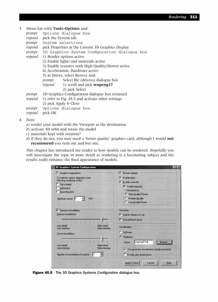
3 Menu bar with Tools-Options and:prompt Options dialogue boxrespond pick the System tabprompt System selectionsrespond pick Properties at the Current 3D Graphics Displayprompt 3D Graphics System Configuration dialogue boxrespond 1) Render options active
2) Enable lights and materials active3) Enable textures with High Quality/Slower active4) Acceleration: Hardware active5) at Driver, select Browse and:prompt Select file (drivers) dialogue boxrespond 1) scroll and pick wopeng17
2) pick Selectprompt 3D Graphics Configuration dialogue box returnedrespond 1) refer to Fig. 45.5 and activate other settings
2) pick Apply & Closeprompt Options dialogue boxrespond pick OK
4 Now: a) render your model with the Viewport as the destination b) activate 3D orbit and rotate the model c) materials kept with rotation?d) if they do not, you may need a ‘better quality’ graphics card, although I would not
recommend you rush out and but one.
This chapter has introduced the reader to how models can be rendered. Hopefully youwill investigate the topic in more detail as rendering is a fascinating subject and theresults really enhance the final appearance of models.
Rendering 311
Figure 45.5 The 3D Graphics Systems Configuration dialogue box.
modelling with AutoCAD.qxd 17/06/2002 15:43 Page 311

Publishing to the webAutoCAD 2002 allows the user to create Web pages of existing drawings. Todemonstrate the concept:
1 Open any model (3D or solid) and:a) activate the Model tabb) view the model in 3Dc) save with a suitable name and note the name
2 Repeat step 1 for some other models (3 or 4)
3 Start a new metric drawing from scratch to display the typical AutoCAD 2002 blankscreen
4 Menu bar with File-Publish to Web and:prompt Publish to Web (Begin) dialogue box (as Layout dialogue box)respond 1. pick Create New Web Page
2. pick Newprompt AutoCAD message similar to Fig. 46.1respond 1. read the message
2. pick Cancel
Figure 46.1 The AutoCAD message with Publish to Web.
Chapter 46
modelling with AutoCAD.qxd 17/06/2002 15:43 Page 312

5 Now open one of the previously opened/saved drawings, then menu bar with File-Publish to Web and:prompt Publish to Web (Begin) dialogue boxrespond 1. pick Create New Web Page
2. pick Newprompt Publish to Web (Create Web Page) dialogue boxrespond 1. Web page name: enter MYSOLID
2. Note parent directory3. Add any suitable description – Fig. 46.24. pick Next
prompt Publish to Web (Select Image Type) dialogue boxrespond 1. select type from list : DWF
2. pick Nextprompt Publish to Web (Select Template) dialogue boxrespond 1. select a template type, e.g. Array plus Summary
2. pick Nextprompt Publish to Web (Apply Theme) dialogue boxrespond 1. scroll and select an element, e.g. Ocean Waves – Fig. 46.3
2. pick Nextprompt Publish to Web (Enable i-drop) dialogue boxrespond activate enable i-drop then pick Nextprompt Publish to Web (Select Drawings) dialogue boxwith the opened drawing listed by namerespond 1. Layout: select Model (probably active)
2. Label: alter to some suitable name3. Description: enter to suit4. pick Add->
and entered label added to Image listrespond pick the (...) at Drawingprompt Publish to Web dialogue box with *.dwg file typerespond 1. scroll to your named folder if not active
2. open another drawing/activity3. Layout: Model4. Label: alter to suit5. Description: enter to suit6. pick Add->
then select (...) another 2/3 drawings and repeat the above six responsesand dialogue box similar to Fig. 46.4then pick Nextprompt Publish to Web (Generate Images) dialogue boxrespond 1. Regenerate images for drawing (etc) active
2. pick Nextprompt Plot progress information displayedthen Publish to Web (Preview and Post) dialogue boxrespond pick Previewand Internet Explorer with Images of drawings – Fig. 46.5respond 1. view your images
2. close the Internet to return to AutoCADand select Finish
6 You have now create a web page which can be:a) edited to your requirementsb) posted to the Internet
7 I hope that in this chapter the user has realised that AutoCAD 2002 has uses other thandrawing. The web page creation is very useful and relatively simple to create
Publishing to the web 313
modelling with AutoCAD.qxd 17/06/2002 15:43 Page 313

314 Modelling with AutoCAD 2002
Figure 46.3 The Publish to Web (Apply Theme) dialogue box.
Figure 46.2 The Publish to Web (Create Web Page) dialogue box.
modelling with AutoCAD.qxd 17/06/2002 15:43 Page 314
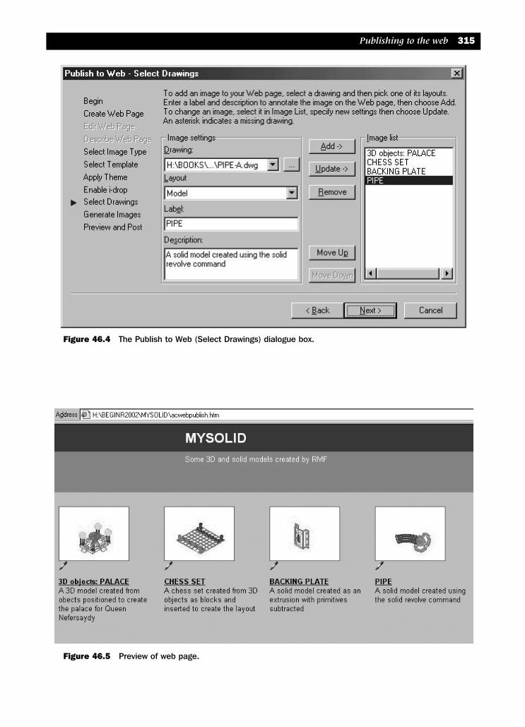
Publishing to the web 315
Figure 46.5 Preview of web page.
Figure 46.4 The Publish to Web (Select Drawings) dialogue box.
modelling with AutoCAD.qxd 17/06/2002 15:43 Page 315
Students’ modelsThis last chapter will show the reader some solid models which have been created bystudents. Motherwell College offers the HNC and HND courses in Computer AidedDraughting and Design, and one of the units on this course requires the students tocomplete a CADD related project. The student must ‘think up’ this project for themselves,produce a brief, produce a technical report and also deliver an oral presentation to theirclass group.
Many different and varied projects are produced including menu customisation, hatchpattern customisation, slide shows etc, but most students decide on solid modelling. The‘object’ which has to be model has to have sizes and the student must obtain these andthen decide on the best way to model the object, i.e. from primitives, regions etc.
To show the reader what can be obtained with solid modelling I have included 12 studentprojects. These are:
Figure Title Student47.1 Anglepoise Lamp John-Joseph McCaveny47.2 Chieftain Tank Joe Williams47.3 Formula 1 Racing Car Tom Doyle47.4 Crash Helmet (Surface model) Steven Anderson-Sams47.5 Micrometer Pamela Hettrick47.6 Wood Plane Michael Monaghan47.7 Droid Ryan Farnin47.8 Suspension Assembly Alan Thomas47.9 Battle Car Craig Matthewman47.10 Vice Keith Irwin47.11 Watch William Milne47.12 3D Chess Set Gary Jamieson
Further student work can be viewed from the Motherwell College website, the addressbeing www.motherwell.co.uk
Chapter 47
modelling with AutoCAD.qxd 17/06/2002 15:43 Page 316

Students’ models 317
Figure 47.1 JJ McCaveny CAD Project.
Figure 47.2 Jow Williams HNC (C) CAD Project (Chieftain tank).
modelling with AutoCAD.qxd 17/06/2002 15:43 Page 317

318 Modelling with AutoCAD 2002
Figure 47.3
Figure 47.4 Steven Anderson-Sams HNC CADD Project.
modelling with AutoCAD.qxd 17/06/2002 15:43 Page 318

Students’ models 319
Figure 47.5
Figure 47.6
modelling with AutoCAD.qxd 17/06/2002 15:43 Page 319

320 Modelling with AutoCAD 2002
Figure 47.7
Figure 47.8
modelling with AutoCAD.qxd 17/06/2002 15:43 Page 320
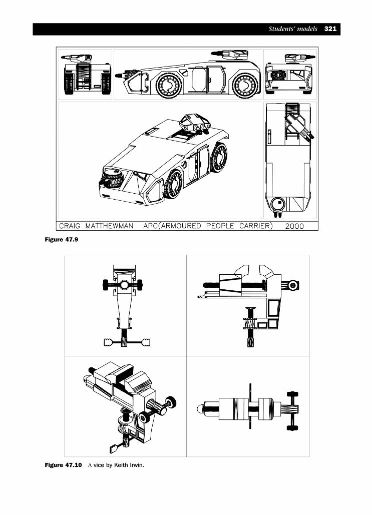
Students’ models 321
Figure 47.9
Figure 47.10 A vice by Keith Irwin.
modelling with AutoCAD.qxd 17/06/2002 15:43 Page 321

322 Modelling with AutoCAD 2002
Figure 47.11
Figure 47.12 Gary Jamieson.
modelling with AutoCAD.qxd 17/06/2002 15:43 Page 322
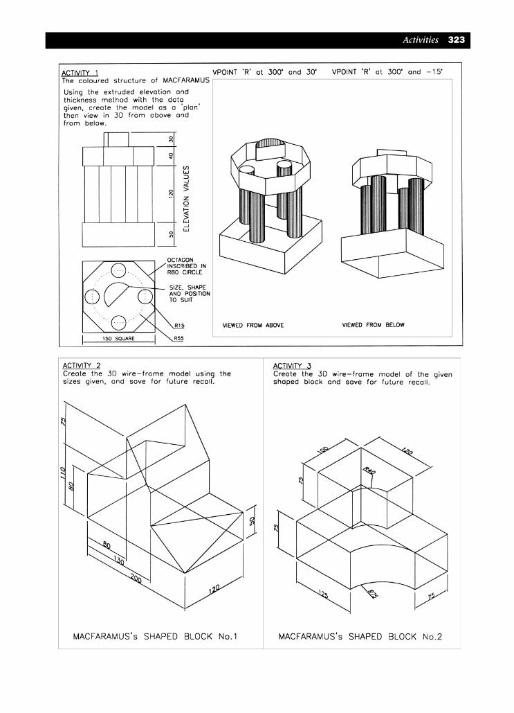
Activities 323
modelling with AutoCAD.qxd 17/06/2002 15:43 Page 323

324 Modelling with AutoCAD 2002
modelling with AutoCAD.qxd 17/06/2002 15:44 Page 324
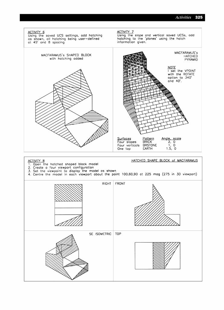
Activities 325
modelling with AutoCAD.qxd 17/06/2002 15:44 Page 325

326 Modelling with AutoCAD 2002
modelling with AutoCAD.qxd 17/06/2002 15:44 Page 326
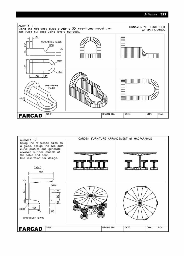
Activities 327
modelling with AutoCAD.qxd 17/06/2002 15:44 Page 327
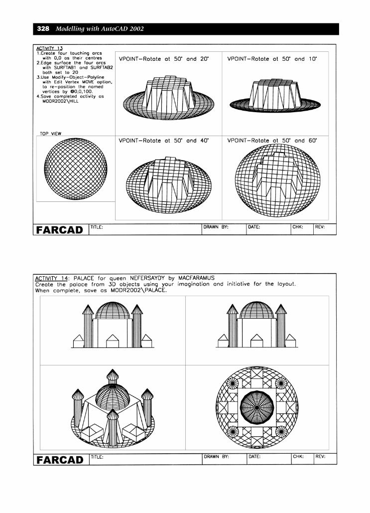
328 Modelling with AutoCAD 2002
modelling with AutoCAD.qxd 17/06/2002 15:44 Page 328

Activities 329
modelling with AutoCAD.qxd 17/06/2002 15:44 Page 329

330 Modelling with AutoCAD 2002
modelling with AutoCAD.qxd 17/06/2002 15:44 Page 330

Activities 331
modelling with AutoCAD.qxd 17/06/2002 15:44 Page 331

332 Modelling with AutoCAD 2002
modelling with AutoCAD.qxd 17/06/2002 15:44 Page 332

Activities 333
modelling with AutoCAD.qxd 17/06/2002 15:44 Page 333

334 Modelling with AutoCAD 2002
modelling with AutoCAD.qxd 17/06/2002 15:44 Page 334

3D Array 1443D Coordinate entry 203D extend and trim 1483D orbit 1743D point UCS 34
Align 146AMBIGUITY 7, 13, 181Area 242Array with 3D 45AutoCAD Design Center 159AutoCAD’s house 162
Background 307Bezier curve 132Bitmap image 308Boundary 235, 238Box primitive 185
Centring models 78CHANGE or CHPROP 186Check 233Clean 233Clipping planes 177Closed paths 114 Color edges/faces 233Cone primitive 190COONS patch 131Copy 3D Models 44Copy faces 233Cubic B spline 12Cylinder primitive 188
Dialogue boxes3D Graphics Systems 311Block definition 153Boundary creation 239Boundary error 53Design center 159New view 76Properties 10Publish to Web 312, 314, 315Render 302UCS 38, 39, 41
UCS Icon 16Use a template 96View 76Viewports 59, 76Viewports preset 67Write block 157Xref manager 283
DIMASSOC 264DIMLFAC 264DISPSILH 194Drawing (setup) 286, 289Dynamics view options 164
ELEVATION 5Extruded faces 226Extruded solids 196
FACETS 100FACETRES 183Floating viewports 56
Global layers 170Gourand shading 8, 99
Handle 255
Icon display 15, 83IMPRINT 232Interactive viewports 56Interference 276Intersection 206Invisible 3D face 104ISOLINES 183Isometric viewport 72
Layer states 171Layout tabs 84, 92Lights 303Loops 235
Mass properties 242Mass properties file 244Materials 307Mirror 3D 142
Index
modelling with AutoCAD.qxd 17/06/2002 15:44 Page 335

Mirror with models 46Model vs paper space 90Moving a UCS 35MVIEW 203
Object UCS 34Offset faces 229Open paths 114Orthographic UCS 40Orthographic viewports 73
Paper space dimensioning 263PICKFIRST 13, 186Plan (UCS) 42Plotting multiple viewports 203Polygonal viewport 95Presets dialogue box 66Profile explanation 259
Revolved solids 201Rotate 3D 140Rotate 3D models 45Rotate faces 230
Scene 303Separate 233Shell 233Solid Modelling 180Sphere primitive 192Spline 130Subtraction 206Surface modelling 180SURFTAB1 114, 121, 127SURFTAB2 123, 127, 132SURFTYPE 132
Taper faces 229THICKNESS 5
TILEMODE 56, 83Toolbars
3D Orbit 178UCS 37View 78
Torus primitive 193True associativity 265True shapes 259, 271
UCS axis rotate 34UCS dialogue box 38UCS Icon 17UCS movement 26UCS new position 33UCS options 36UCS orientation 20UCS specific commands 41UCS FOLLOW 43UCS UP 61, 84Union 206Untitled viewports 85User coordinate system 15
View (setup) 286, 287VIEW command 75View UCS 34Viewpoint compass 68Viewpoint plan 74Viewpoint rotate 64Viewpoint vector 70Viewport configuration 56Viewport specific layers 170, 263
Wedge primitive 187Wireframe modelling 180World coordinate system 14
Z axis vector 33
336 Modelling with AutoCAD 2002
modelling with AutoCAD.qxd 17/06/2002 15:44 Page 336

modelling with AutoCAD.qxd 17/06/2002 15:44 Page 337

modelling with AutoCAD.qxd 17/06/2002 15:44 Page 338

modelling with AutoCAD.qxd 17/06/2002 15:44 Page 339

modelling with AutoCAD.qxd 17/06/2002 15:44 Page 340

modelling with AutoCAD.qxd 17/06/2002 15:44 Page 341

modelling with AutoCAD.qxd 17/06/2002 15:44 Page 342

modelling with AutoCAD.qxd 17/06/2002 15:44 Page 343

modelling with AutoCAD.qxd 17/06/2002 15:44 Page 344