modelling the impact of treatment uncertainties in
TRANSCRIPT

Modelling the impact of treatment
uncertainties in radiotherapy
Jeremy T. Booth, B.MedPhys(Hons)
Supervisors:
Dr. Sergei F. Zavgorodni
Dr. John R. Patterson
A thesis submitted for the degree of
Doctor of Philosophy
in the Department of Physics and Mathematical Physics
University of Adelaide
~ March 2002 ~

ii

iii
Table of Contents
TABLE OF CONTENTS ........................................................................................................................ III
ABBREVIATIONS AND ACRONYMS.............................................................................................. VIII
SYMBOLS ................................................................................................................................................X
LIST OF FIGURES ..............................................................................................................................XIV
LIST OF TABLES .............................................................................................................................XVIII
ABSTRACT ..........................................................................................................................................XIX
THESIS STATEMENT ........................................................................................................................XXI
ACKNOWLEDGEMENTS ................................................................................................................ XXII
CHAPTER 1 GENERAL INTRODUCTION 1 1.1. EXTERNAL BEAM RADIOTHERAPY PLANNING 1 1.2. AIMS OF CURRENT INVESTIGATION 4 1.3. THESIS OUTLINE 5 1.4. PUBLICATIONS 6 CHAPTER 2 A REVIEW OF PATIENT POSITIONING UNCERTAINTY AND ORGAN MOTION AT VARIOUS ANATOMICAL SITES 9 2.1. INTRODUCTION 9 2.2. REVIEW OF ICRU REPORTS 50 AND 62 10 2.3. COMPARISON ACROSS STUDIES 12 2.4. PATIENT POSITIONING (SETUP) ERRORS 14
2.4.1. Defining Patient Positioning Errors 14 2.4.2. Magnitudes of positioning errors at various sites 16 2.4.3. Patient Immobilisation 18 2.4.4. Pelvis 18 2.4.5. Brain 20 2.4.6. Abdomen 20 2.4.7. Head and Neck 20 2.4.8. Breast 21
2.5. ORGAN MOTION 21 2.5.1. Defining organ motion 21

iv
2.5.2. Magnitudes of organ motion 22 2.5.3. Prostate Motion 23
2.5.3.1. Supine versus prone treatment positions 25 2.5.3.2. Bladder/rectum filling influence on prostate motion (MODprostate) 25 2.5.3.3. Strategies to account for prostate motion 27
2.5.4. Abdominal Motion 28 2.5.4.1. Generalities 28 2.5.4.2. Kidney Motion 30 2.5.4.3. Diaphragm Motion 30 2.5.4.4. Pancreas Motion 31 2.5.4.5. Breath Holding Techniques 31 2.5.4.6. Advanced Techniques 31 2.5.4.7. Patient Orientation during treatment 32
2.6. PATIENT REPOSITIONING STRATEGIES 32 2.7. CONTEMPORARY SUGGESTIONS FOR TREATMENT PLANNING 35
2.7.1. Statistics based treatment margins 35 2.7.2. Adaptive radiation therapy 39 2.7.3. Monte Carlo techniques 40 2.7.4. Convolution techniques 41
2.8. SUMMARY 42 CHAPTER 3 REVIEW OF RADIOBIOLOGICAL MODELS 43 3.1. INTRODUCTION 43 3.2. BIOLOGICAL MODELS 44
3.2.1. Empirical (Logit and Probit) Models 44 3.2.2. Theoretical (Poisson/Linear Quadratic) Model 45 3.2.3. Hyper sensitivity of tumour/normal tissue at low doses 48 3.2.4. Biological Effective Dose 49 3.2.5. Standard Effective Dose 50 3.2.6. Equivalent Uniform Dose 50
3.3. TUMOUR CONTROL PROBABILITY 51 3.3.1. Accounting for interpatient radiosensitivity variation in a population of patients 52 3.3.2. Clonogen denisity and optimisation 52 3.3.3. Prostate Carcinoma 54
3.4. NORMAL TISSUE COMPLICATION PROBABILITY 55 3.4.1. Dose-Volume effects 55 3.4.2. Lyman-Kutcher-Burman (LKB) model 56 3.4.3. Källman k- and s-models 59 3.4.4. Yaes-Kalend/Fenwick model 60 3.4.5. Clinical application of NTCP 61 3.4.6. Rectal complications 62
3.4.6.1. Grading rectal complications 62 3.4.6.2. Rectum architecture 62 3.4.6.3. Dose volume characterisation 64
3.5. UNCOMPLICATED TUMOUR CONTROL AND OBJECTIVE FUNCTIONS 67 3.6. SUMMARY 69 CHAPTER 4 MODELLING THE DOSIMETRIC EFFECT OF TREATMENT UNCERTAINTY 71
v
4.1. INTRODUCTION 71 4.2. DOSE UNCERTAINTY 72
4.2.1. Modelling dose uncertainty 73 4.2.2. Probability density functions for position and dose 73
4.3. MONTE CARLO TECHNIQUE 76 4.3.1. Methods 76
4.3.1.1. Sampling from distributions, and the dose grid 77 4.3.1.2. Dose accumulation 78 4.3.1.3. Clinical example 79
4.3.2. Results 80 4.3.2.1. Mean and variance in fractionated dose for single incident beam 80 4.3.2.2. Impact of margin size 83 4.3.2.3. Impact of magnitude of patient positioning and organ variations 83 4.3.2.4. Number of fields and dose gradients. 83
4.3.3. Discussion 85 4.3.3.1. Possible margin reductions with multiple pretreatment CT scans 85 4.3.3.2. Relative importance of systematic and random components 85 4.3.3.3. Comparison of spatially uniform dose error and positioning errors 86 4.3.3.4. Dose reporting 87
4.4. CONVOLUTION TECHNIQUE 87 4.4.1. Derivation of spatial PDF including systematic organ motion error 88 4.4.2. Benchmarking against Monte Carlo results 89 4.4.3. Margin recipe including systematic error 89
4.5. MULTIPLE CT SCANS 90 4.5.1. Timing regimes for multiple intra-treatment image acquisition 90 4.5.2. Results 92
4.6. MONTE CARLO MODELLING OF 3D DOSIMETRIC IMPACT 92 4.6.1. Methods 92 4.6.2. Results 95 4.6.3. Discussion 97
4.7. SUMMARY AND CONCLUSION 99 CHAPTER 5 MODELLING DOSE DEPOSITION TO THE DEFORMING RECTUM 101 5.1. INTRODUCTION 101 5.2. BACKGROUND 102 5.3. METHODS 104
5.3.1. ‘Original’ and ‘Initial’ rectum geometries 104 5.3.1.1. Original geometry 104 5.3.1.2. Initial Geometry 106
5.3.2. Modelling rectum deformations 107 5.3.3. Modelling planning CT image acquisition 109 5.3.4. Modelling treatment delivery 112 5.3.5. The input data 113
5.3.5.1. Geometry 113 5.3.5.2. Uncertainty parameters 114
5.3.6. Calculations 114 5.4. RESULTS 115
5.4.1. Planned rectum dose distributions 115 5.4.2. Interfraction variations 117
5.4.2.1. Systematic error: empty rectum at planning 117 5.4.2.2. Systematic error: full rectum at planning 120

vi
5.4.3. Interpatient variations 121 5.5. DISCUSSION 128 5.6. CONCLUSIONS 130 CHAPTER 6 MODELLING THE RADIOBIOLOGICAL EFFECT OF TREATMENT UNCERTAINTY IN RADIOTHERAPY 133 6.1. INTRODUCTION 133 6.2. TUMOUR CONTROL PROBABILITY 133
6.2.1. Background 134 6.2.2. Method 134
6.2.2.1. Input data for 1D case 136 6.2.2.2. Input data for 3D case 138 6.2.2.3. Calculations 138
6.2.3. Results 139 6.2.3.1. Impact of margin size 139 6.2.3.2. Impact of penumbra steepness 141 6.2.3.3. Impact of uniform dose uncertainty and interpatient heterogeneity 143 6.2.3.4. Results using 3D input data 149
6.2.4. Discussion 151 6.3. NORMAL TISSUE COMPLICATION PROBABILITY 154
6.3.1. Background: Incorporating treatment uncertainty into NTCP calculation 154 6.3.2. Methods 155
6.3.2.1. Fitting Linear-Quadratic parameters to late rectum complications 155 6.3.2.2. Modelling individual treatments and patient populations 156
6.3.3. Results 156 6.3.3.1. Individual patients 156 6.3.3.2. Population based results 158 6.3.3.3. Impact of fluctuations in fractional dose 158 6.3.3.4. Comparison with mean treatment dose 160
6.3.4. Discussion 162 6.4. UNCOMPLICATED TUMOUR CONTROL PROBABILITY (UTCP) 165
6.4.1. Methods 165 6.4.2. Results 166
6.4.2.1. UTCP calculated for an individual patient 166 6.4.2.2. Population based results 167
6.4.3. Discussion 171 6.5. CONCLUSIONS 173
CHAPTER 7 TREATMENT PLANNING ALGORITHM CORRECTIONS TO ACCOUNT FOR AND DISPLAY DOSE UNCERTAINTY IN RADIOTHERAPY 175 7.1. INTRODUCTION 175
7.1.1. Possibilities for future radiotherapy treatment planning 175 7.1.2. Purpose 176
7.2. MODIFICATIONS TO DOSE CALCULATION ALGORITHMS FOR PHOTONS 177
7.1.3. Correction based techniques 177 7.2.1.1. Input data 177 7.2.1.2. Dose calculation 178 7.2.1.3. Including estimations of error 180
7.1.4. Superposition technique 180

vii
7.2.1.4. Input data 180 7.2.1.5. Dose calculation 180 7.2.1.6. Including estimations of error 181
7.1.5. Monte Carlo technique 183 7.2.1.7. Input data 183 7.2.1.8. Dose calculation 183 7.2.1.9. Including estimations of error 184
7.3. REQUIREMENTS FOR DISPLAY INPUT DATA 185 7.1.6. Standard deviations 185 7.1.7. Non standard deviations 186
7.4. TREATMENT PLANNING DISPLAYS 187 7.1.8. Mean dose and/or standard deviation 187 7.1.9. Modified dose volume histogram 190 7.1.10. Mean with estimated standard deviation display 190 7.1.11. Difference maps 192
7.5. CRITICAL EVALUATION OF UNCERTAINTY DISPLAY TOOLS 193 7.6. CONCLUSIONS 196
CHAPTER 8 CONCLUSIONS AND FURTHER RESEARCH 197 8.1. MAJOR CONCLUSIONS 198 8.2. FURTHER RESEARCH 201 Appendix A 203
References 223

viii
Abbreviations and Acronyms AP Anterior-Posterior direction BED Biological Effective Dose
CL-DVH Confidence Limited Dose Volume Histogram CT Computed Tomography
CTV Clinical Tumour Volume DNA Deoxyribose Nucleic Acid
DSAR Differential Scatter Air Ratio DVH Dose Volume Histogram
DWH Dose Wall Histogram EGS4 Electron Gamma Shower version 4
EPID Electronic Portal Imaging Device ETAR Equivalent Tissue Air Ratio
EUBED Equivalent Uniform Biologically Effective Dose EUD Equivalent Uniform Dose
FFT Fast Fourier Transform FML Full Maximum Likelihood
FS Field Size FSU Functional Sub-Unit
FWHM Full Width at Half Maximum GTV Gross Tumour Volume
HDSA High Dose Surface Area I-125 Iodine-125
ICRU International Commission on Radiation Units IM Internal Margin
IMRT Intensity Modulated Radiation Therapy IPTV Internal Planning Target Volume
IR Induced Repair LET Linear Energy Transfer
LQ Linear Quadratic LR Left-Right direction
MC Monte Carlo ML Medio Lateral (same plane as left right)

ix
MOD Mean Organ Displacement
MRI (nuclear) Magnetic Resonance Imaging MTPD Mean Treatment Position Deviation
NAL No Action Level NTCP Normal Tissue Complication Probability
OAR Organ At Risk PDF Probability Density Function
PDV Prescribed Dose Volume PTV Planning Target Volume
RTOG Radiation Therapy Oncology Group grading system RTP Radiation Therapy Planning
SAL Shrinking Action Level SD Standard Deviation
SEAS Setup Error (averaged) Across Studies SED Standard effective dose
SI Superior-Inferior direction SM Setup Margin
SSD Surface-Skin Distance TCP Tumour Control Probability
TERMA Total Energy Released in the Medium TPD Treatment Position Deviation
TPS Treatment Planning System UTCP Uncomplicated Tumour Control Probability

x
Symbols
ξ mean organ position
x mean patient position based on all measurements for a group of patients
r mean rectal wall radius across Nz CT slices
popr mean rectal wall radius across patient population
D mean treatment dose
)(rd s∗ perturbed sample fraction dose in spatial element ∆r located ∆r +r units from the
isocentre
jx∆ systematic patient positioning error for jth patient
τ initial action level for possible patient repositioning
ϕ proportion of patients with injury uncorrelated to benefit
φj random deviate from Gaussian distribution describing patient position at the jth fraction dose
σm,organ standard deviation in mean organ position
σR,j standard deviation of random error for jth patient
ΣT standard deviation of systematic setup error across a group of patients
∆xi,j measured shift in patient position in ith portal image from position at simulation for jth patient a variable
A0 (original) area of rectal wall segment b variable
ca partial score (for treatment plan) Ci score
CT∞ infinite CT images used to calculate true mean organ position d fraction dose D treatment dose including, for example, 30 fraction doses
D0 planned treatment dose D50 dose that produces a given endpoint in 50% of the population after 5 years
dc dose limit for induced repair deff effective depth
Dm Maximum treatment dose dmax depth of maximum dose

xi
ds fraction dose sampled from known distribution
Ds(r) sum of Nfx sample fraction doses ds
* perturbed fraction dose
dst standard dose per fraction (Gy) d㦀 angle increment
E rotation vector erf() error function
F objective function g Gaussian function
GC (absolute) position of geometric centre of rectum H CTV→PTV margin
Hp primary kernel
Hs scatter kernel k parameter from Kallman k-model
m parameter from Lyman model M the total number of voxels
N a number (general) n parameter from Lyman model
N0 initial number of cells in tumour/organ Ncell number of consecutive cells
NCT the number in CT image acquisitions NF number of FSU’s in organ
NFSU number of cells per FSU Nfx the number of fraction doses
nj number of portal images Npat number of patients in a particular study
NS number of surviving cells following irradiation NSD
number of standard deviations Nz number of slices in CT image set
P probability (general)
P(D,1) dose-response function, giving the probability of a given endpoint following irradiation of whole organ volume
P(D,v) dose-response function, giving the probability of a given endpoint following irradiation of partial volume
P+ probability of uncomplicated tumour control

xii
PB probability of benefit from the treatment
PB|I conditional probability for benefit without injury PI probability of treatment induced injury
r radius (general)
r0 initial rectal radius
ξ random deviate from Gaussian distribution describing organ position rdef radius of deformed rectal wall rin inner rectal wall radius
s parameter from Kallman s-model S surviving fraction
T TERMA (see abbreviations) T total time of treatment (days)
T1/2 half-life for sub lethal damage Tk kick-off time (days)
Tpot potential doubling time of tumour (days) U Utility of treatment
ut vector displacement at time, t. v partial volume (cm3)
Veff effective volume (considering tissue architecture) (cm3)
Vt tumour volume (cm3)
w rectal wall thickness (mm). w′ weighted change in rectal wall thickness
x position along LR axis (mm).
x0(v) position (absolute) of v at planning (mm). xt(v) position (absolute) of v at time, t (mm).
y position along AP axis (mm). z position along SI axis (mm).
㬰 gradient of dose response function 㥀 deviation or shift (of dose distribution) (mm).
㥀r change in rectum radius (mm).
㥀v sub-volume (normally volume of a voxel)
㥀w change in rectal wall thickness (mm).
㭠 random deviate sampled from Gaussian distribution

xiii
㭰 co-efficient
㦀 angle 㯀 on-going number of measurement
㯠 organ position (mm).
㲐 a weighting factor
∆j total shift from mean organ position for jth fraction (mm).
∆r′ weighted change in radius
Σ standard deviation between patient variables (systematic error)
Σdelin standard deviation in interpatient (systematic) mean delineation error
ΣOM standard deviation in interpatient (systematic) mean organ motion error
ΣSE standard deviation in interpatient (systematic) mean setup error
α parameter of the Linear Quadratic model for cell killing (Gy-1)
αs hyper sensitive cell sensitive at low dose (Gy-1)
β parameter of the Linear Quadratic model for cell killing (Gy-2)
ρ clonogen density (cm-3)
σ standard deviation in random parameter (general)
σOM standard deivation in interfraction (random) organ motion
σp standard deviation describing the production of penumbra
σSE standard deviation in interfraction (random) setup error
σTD standard deviation of treatment delivery (random) errors (i.e. interfraction setup errors plus interfraction organ motion error)
σα standard deviation in interpatient (systematic) cell sensitivity

xiv
List of Figures Figure 2.1 Definitions of treatment volumes as defined by ICRU-62 (Fig. 2.16) showing their relation by scenarios A, B and C discussed in the text.
Figure 2.2 Cumulative probability distributions as a function of the normalised radius of expansion for three different CTV-PTV margin strategies. From Antolak and Rosen (1999).
Figure 3.1 Plots of Probability of effect following single fraction irradiation to dose, as calculated with the Probit model (solid curve) and Logit model (dashed).
Figure 3.2 Surviving fraction versus dose for early responding tumour tissue and late responding normal tissue. Tumour is characterised by α= 0.35 Gy-1 and α/β = 10, while normal tissue is characterised by α = 0.15 Gy-1 and α/β = 3 (from Metcalfe et al. 1997).
Figure 3.3 Survival fraction versus dose for T98G human glioma cells. The dots with error bars are the experimental data points, the dashed curve is the LQ model prediction, and the solid curve is the IR model prediction. From Joiner et al. (2001).
Figure 3.4 Characteristic sigmoidal TCP versus dose curve derived theoretically and experimentally. (Taken from Webb and Nahum 1994)
Figure 3.5 The dose-volume relationship for a) the (mostly serial) esophagus, b) for (mostly parallel) lung, and c) for the rectum. Taken from Burman et al. (1991) using data from Emami et al. (1991).
Figure 3.6 a) The distribution of rectal surface area irradiated across patients can be separated by the grade of prostate cancer. Taken from Lu et al. (1995) b) The correlation between NTCP and volume is strongest at low partial volumes (less than 0.5) and for full volume delineation. Taken from Dale et al. (1999).
Figure 3.7 A transverse section of the rectum showing different methods of organ delineation for generating histograms. Adapted from Dale and Olsen (1998).
Figure 3.8 Characterisation of the Dose Surface Histogram. From Fenwick et al. (2001).
Figure 4.1 Demonstration of the direct derivation of dose PDF from spatial PDF with static dose distribution. (Adapted from Leong 1987). The spatial PDF (below the half dose profile) is used to allocate probability values (a dose PDF located right of the half dose profile) for a particular element of radius positioned originally at 50% dose. This procedure is repeated for other elements yielding dose PDFs as shown in figure 4-2 below.
Figure 4.2 Dose PDFs within voxels that are positioned at five distances from the central axis, labelled from Figure 4.1. Only odd numbered curves are shown for brevity. Dose PDF curves for distances 3 and 5 cm (corresponding to radii r3 and r5 respectively) predict mainly high and low doses respectively because these voxels are centred at the upper and lower position of the dose profile. The dose PDF curve for the voxel centred at 4 cm from the central axis (radius r4) is smeared over a large dose range because it’s mean location is the midpoint of the penumbra. The value of the positional PDF standard deviation is 0.6 cm.
Figure 4.3 Rayleigh distribution with b=2.
Figure 4.4 Maxwell probability density function with b=2.
Figure 4.5 (a) Mean organ position is represented by the x,y co-ordinate system. In routine treatment, due to CT uncertainty, the planning image represents the organ in an off-set co-ordinate system (the x′,y′ co-ordinate system). This co-ordinate system is then used to plan and deliver the dose. The 1D approach in this study uses only the x-component of these 2D shifts. (b) Organ positions during the treatment delivery (such as φ1, φ2 and φ3 for 3 fractions) are measured in the off-set (x′,y′) co-ordinate system.
Figure 4.6 (a) Mean dose incorporating uncertainty at both planning and treatment. The dose profile represented by the broken line is the original dose profile and that represented by a solid line includes only the treatment delivery errors. The spatially uniform dose uncertainty follows the original dose profile. (b) Magnified view of penumbra.
xv
Figure 4.7 Dose variation (1 standard deviation of mean treatment dose) scored in voxels (∆x = 0.1 cm), using multiple CT scans to estimate mean organ position. The solid line shows dose variation due only to treatment delivery uncertainty. Vertical lines represent position of 95% isodose contour and the dash-dot line represents the spatially uniform dose uncertainty.
Figure 4.8 a) One dimensional profiles of prescribed dose distributions with three margin sizes (0.5, 1.0, 1.5 cm) and b) the associated standard deviations in treatment dose.
Figure 4.9 Standard deviation in treatment dose using the standard deviation in position to be 0.6, 0.8 and 1.0 cm. The value given as ‘tumour position’ is the standard deviation equal to the quadratic sum or random inter-fraction organ motion and random setup errors.
Figure 4.10 Possible reductions in margin size evident from improving knowledge of mean organ position.
Figure 4.11 Mean treatment dose predicted for 1 and 5 CT scans using the convolution method as compared with MC results. The original dose profile is also shown.
Figure 4.12 Flow chart of regimes for timing multiple imaging
Figure 4.13 Mean dose (A→C) and variance in mean dose (D→F) resulting from incorporating regimes A,B, C into Monte Carlo modelling of the treatment process.
Figure 4.14 Illustration of the prostate gland (GTV), rectum and three dose distributions characterised by margins of a) 0.5 cm b) 1.0 cm and c) 1.5 cm. In each case the 95% isodose indicates the PTV, the green volume is the prostate (GTV & CTV) and the brown volume is the rectal wall.
Figure 4.15 Two views of the mean treatment dose calculated with three original dose distributions (for margins of 0.5, 1.0, 1.5 cm) for three cases. The three cases are an original dose distribution (black solid line), a mean treatment dose calculated based on 1 planning CT scan (blue solid) and a mean treatment dose based on infinite planning CT scans (red dashed line).
Figure 4.16 Iso-standard deviation plots in the transverse plane with a) 0.5 cm and b) 1.5 cm margin.
Figure 4.17 Profiles of one standard deviation in mean treatment dose along the lateral (X) and anterior-posterior (Y) direction for the a) 0.5 cm margin, b) 1.0 cm margin and c) 1.5 cm margin.
Figure 5.1 Schematic of the characterisation of the rectum geometry A rectal wall segment will area, A0, subtended by dθ of distance rin(θ) from the geometric centre, and of thickness, w(θ).
Figure 5.2 Plot of inner rectum wall radius, and wall thickness versus angle for a characteristic slice.
Figure 5.3 Calculated wall thickness (Eq.5.7) with changes of rectal wall radius..
Figure 5.4 Rectum segment has constant area. Dashed segment is original segment.
Figure 5.5 Modelling shifts of the rectum GC is done by shifting the entire organ within a fixed dose grid. A) The rectum GC position in the original CT planning image is compared to b) the position(shifted posteriorly) in a later fraction, or CT image acquisition.
Figure 5.6 Dose surface histograms of the planned dose distributions with CTV-PTV margins of 5, 10, or 15 mm.
Figure 5.7 Dose Surface maps of the planned dose distributions with CTV-PTV margins of a) 5 mm, b) 10 mm, or c) 15 mm. Orientation: Left=0°; Anterior=90°.
Figure 5.8 DSH showing the mean and planned dose distributions modelling an empty rectum at planning with three CTV-PTV margins.
Figure 5.9 Dose Surface Maps showing the difference between rectal dose distributions with empty rectum at planning for a) 5 mm margin, b) 10 mm margin, c) 15 mm margin. Orientation: Left=0°; Anterior=90°.
Figure 5.10 DSH for planned and mean (calculated) dose distributions with 5, 10, and 15 mm margins, including a full rectum at planning.
Figure 5.11 DSM showing where the difference dose occurs for margins of a) 5 mm, b) 10 mm, and c) 15 mm with full rectum at planning. Orientation: Left=0°; Anterior=90°.
Figure 5.12 Dose surface histograms of the rectal wall for dose distributions with a) 5 mm b) 10 mm, and c) 15 mm margin. The three planned dose distributions are solid lines and the 20 DSHs including random and systematic errors are dashed lines. The individual patient DSHs are symmetrical about the planned DSH across the population
A0

xvi
Figure 5.13 The standard deviation in rectal wall dose calculated with 5 mm margin and a) one pre-treatment CT scan with, b) two pre-treatment CT scans, and c) infinite pre-treatment CT scans. Orientation: Left=0°; Anterior=90°.
Figure 5.14 The standard deviation in rectal wall dose calculated with 10 mm margin and a) one pre-treatment CT scan with, b) two pre-treatment CT scans, and c) infinite pre-treatment CT scans. Orientation: Left=0°; Anterior=90°.
Figure 5.15 The standard deviation in dose presented as a DSM. A margin of 15 mm is used with a) one, b) two, and c) an infinite number of pretreatment CT scan information. Orientation: Left=0°; Anterior=90°.
Figure 6.1 Isodose contours for typical prostate treatment. The CTV (solid and filled), PTV (dotted), and rectum (brown) are shown, with the oblique and horizontal lines indicating the position of dose profiles used.
Figure 6.2 The dose distribution for 1D TCP calculations.
Figure 6.3 TCP calculated with planned dose distribution versus mean calculated with CTV-PTV margins of 0.5 cm, 1.0 cm and 1.5 cm (incorporating treatment uncertainty). The magnitude of treatment uncertainty is fixed for all cases.
Figure 6.4 TCP calculated with planned dose distribution versus mode calculated with CTV-PTV margins of 0.5 cm, 1.0 cm and 1.5 cm (incorporating treatment uncertainty). The magnitude of treatment uncertainty is fixed for all cases.
Figure 6.5 Mean TCP calculated using dose distribution with steep penumbra compared with the standard dose distribution.
Figure 6.6 Mean tumour control probability for treatments incorporating non-uniform dose uncertainty, uniform dose uncertainty and varying cell sensitivity inter-patient.
Figure 6.7 Standard deviation in mean tumour control probability incorporating spatially non-uniform dose uncertainty, spatially uniform dose uncertainty and varying cell sensitivity inter-patient.
Figure 6.8 Distributions of TCP for three dose levels a) 48 Gy, b) 52 Gy, and c) 56 Gy incorporating dose uncertainty (uniform or non-uniform) and inter-patient cell sensitivity variation. The exact calculated TCP at these dose levels (shown as vertical dashed line) are 0.05, 0.58 and 0.90, respectively.
Figure 6.9 Mode of TCP over a patient population.
Figure 6.10 TCP calculated for an individual patient with (F)ull or (E)mpty rectum in planning CT scan with margins of 0.5 cm, 1.0 cm, or1.5 cm.
Figure 6.11 Plot of TCP versus cell sensitivity. Two values of cell sensitivity (α 1=0.29 Gy-1, α 2=0.35 Gy-1) and the range covered by one and two standard deviations in cell sensitivity are illustrated. See text for further description.
Figure 6.11 Schematics of voxel-based dose allocation from the deformed rectal wall (dashed) to the original wall (solid) following a sampled change of radius. Three cases are shown, where a) the wall thickness does not change, b) the wall thickness is reduced, and c) where the wall thickness increases. See text for further explanation.
Figure 6.13 Mean NTCP calculated for individual patients with either full (F) or empty (E) rectums in the planning CT scan and with margins of 0.5 cm, 1.0 cm, or 1.5 cm. Table 6.4 NTCP across a patient population (N=1000) with D=64 Gy
Figure 6.14 NTCP calculated with planned dose or with a 5% spatially uniform dose error at each fraction of treatment.
Figure 6.15 Comparison between NTCP calculated with the planned dose distribution against NTCP calculated assuming that the planned surface dose (from DSM) is deposited uniformly in each angular rectal wall segment.
Figure 6.16 Comparison of mean NTCP calculated with mean dose against the calculated rectal wall dose. Both sets were calculated for a population of patients, with each patient being planned from a single CT image set.

xvii
Figure 6.17 Comparison of mean NTCP calculated with the mean dose against the MC calculated rectal wall dose. Both sets were calculated for a population of patients, with each patient being planned using the mean organ position.
Figure 6.18 NTCP calculated using the mean dose with n=0.24, m=0.15 for an individual patient with systematic error.
Figure 6.19 NTCP calculated using the mean dose with n=0.12, m=0.15 for an individual patient with systematic error.
Figure 6.20 Mean UTCP calculated for a population of identical patients with fixed systematic error.
Figure 6.21 Mean UTCP (1CT) versus dose for margin sizes 0.5, 1.0, and 1.5 cm.
Figure 6.22 Mean UTCP against margin size at a) 64 Gy and b) 70 Gy..
Figure 7.1 Correction factors for various inhomogeneity correction techniques versus depth in different density media. Taken from Wong and Purdy (1990).
Figure 7.2 The superposition dose calculation technique models primary fluence interactions at r′ and the probability of dose deposition in surrounding voxels, including that voxel centred at r. Adapted from Metcalfe et al. (1997).
Figure 7.3 The superposition dose calculation overestimates dose in lower density media and underestimates after lower density media. Taken from Metcalfe et al. (1997).
Figure 7.4 Dose PDF at the medial edge of the penumbra.
Figure 7.5 Standard deviation isodoses for a) a liver treatment including random patient positioning errors (Taken from Lujan et al. 1999) and b) a 4-field prostate treatment (reproduced from Chapter 4).
Figure 7.6 a) Mean isodose contours, and b) Confidence limit plot showing the minimum dose received by 90% of the population.
Figure 7.8 The CL-DVH from Mageras et al. (1999) a) for prostate and b) rectum, and b) the DVH accuracy increases with the number of fractions (from Lujan et al. 1999)
Figure 7.9 Schematic of the a) 95% modal isodose, and b) 30% modal isodose with error bars indicating a 95% chance of depositing given dose.
Figure 7.10 Single axial slice showing lateral and AP beam orientation, b) dose difference display: 0DD − . Taken from Lujan et al. (1999).

xviii
List of Tables
Table 2.1 Variation in parameters used for measurement of MODprostate.. Key: full (F) bladder/rectum, empty (E) bladder/rectum, rectum status Not Considered (NC), insufficient information provided (-). The numbers of images taken per patient refers to the number of images (CT, simulation and portals) used to derive their final measurement. Patients were treated in the supine (S) or prone (P) position, whether patient repositioning was done (yes, Y) or was not done (no, N), and the method used for the measurement (M1 or M2) from the text. In two studies the bladder/rectum content was increased with time (*), while in another study two time periods for voiding before treatment were examined (**).
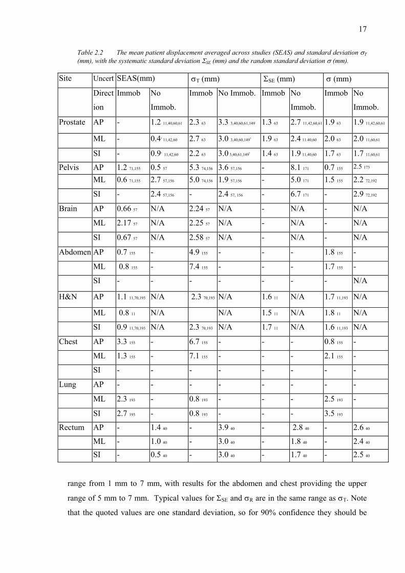
Table 2.2 The mean patient displacement averaged across studies (SEAS) and standard deviation δ (mm), with the systematic standard deviation δS (mm) and the random standard deviation δR (mm).
Table 2.3 Prostate position uncertainty due to the motion not directly attributed to bladder/rectum filling in the anterior-posterior, medio-lateral and superior-inferior directions. References will be bracketed.
Table 2.4 Summary of respiration-induced abdominal motion. The movement of the organ is the positional difference of the organ from inhalation to exhalation, unless otherwise stated. The details of the measurement may include a direction, breathing rate, alternate endpoint, or the condition of the organ at the time of measurement i.e. disease title.
Table 3.1 Magnitudes of parameters m,n,D50, s and k used to model normal tissue complications following full volume irradiation for a range of organs. From Burman et al. (1991) and Kallman et al. (1992).
Table 4.1 Summary of typical error magnitudes concerning supine treatment of prostate carcinoma used for modelling. Delineation error ranges are due to uncertainty in apex and seminal vesicles localisation. Systematic set-up errors quoted do not include the use of a correction protocol.
Table 5.1 The parameters defining systematic and random changes in rectum geometry
Table 6.1 The effect of margin size on TCP incorporating treatment uncertainty. The difference between planned TCP and mean TCP with 1 CT, as well as the difference in TCP between the planned and calculated mean TCP are shown.
Table 6.2 The effect of margin size on TCP incorporating treatment uncertainty and steep dose gradient to mimic IMRT. The difference between planned TCP and mean TCP at a 60 Gy dose level, as well as the difference in dose between the planned and calculated mean TCP at two levels of TCP are shown.
Table 6.3 Mean TCP across a patient population for three margin sizes, with error given as one standard deviation in mean TCP.
Table 6.4 NTCP across a patient population (N=1000) with D=64 Gy
Table 6.5 Maximum value of mean UTCP across a population with 1 SD uncertainty. The dose required for maximum UTCP is given in brackets.

xix
Abstract Uncertainties are inevitably part of the radiotherapy process. Uncertainty in the dose
deposited in the tumour exists due to organ motion, patient positioning errors, fluctuations
in machine output, delineation of regions of interest, the modality of imaging used, and
treatment planning algorithm assumptions among others; there is uncertainty in the dose
required to eradicate a tumour due to interpatient variations in patient-specific variables
such as their sensitivity to radiation; and there is uncertainty in the dose-volume restraints
that limit dose to normal tissue.
This thesis involves three major streams of research including investigation of the actual
dose delivered to target and normal tissue, the effect of dose uncertainty on radiobiological
indices, and techniques to display the dose uncertainty in a treatment planning system. All
of the analyses are performed with the dose distribution from a four-field box treatment
using 6 MV photons. The treatment fields include uniform margins between the clinical
target volume and planning target volume of 0.5 cm, 1.0 cm, and 1.5 cm. The major work
is preceded by a thorough literature review on the size of setup and organ motion errors for
various organs and setup techniques used in radiotherapy.
A Monte Carlo (MC) code was written to simulate both the treatment planning and
delivery phases of the radiotherapy treatment. Using MC, the mean and the variation in
treatment dose are calculated for both an individual patient and across a population of
patients. In particular, the possible discrepancy in tumour position located from a single
CT scan and the magnitude of reduction in dose variation following multiple CT scans is
investigated. A novel convolution kernel to include multiple pretreatment CT scans in the
calculation of mean treatment dose is derived. Variations in dose deposited to prostate and
rectal wall are assessed for each of the margins and for various magnitudes of systematic
and random error, and penumbra gradients.
The linear quadratic model is used to calculate prostate Tumour Control Probability (TCP)
incorporating an actual (modelled) delivered prostate dose. The Kallman s-model is used to
calculate the normal tissue complication probability (NTCP), incorporating actual

xx
(modelled) fraction dose in the deforming rectal wall. The impact of each treatment
uncertainty on the variation in the radiobiological index is calculated for the margin sizes.

xxi
Thesis Statement
This work contains no material which has been accepted for the award of any other degree
or diploma in any University or other tertiary institution and, to the best of my knowledge
and belief, contains no material previously published or written by another person, except
where due reference has been made in the text.
I give consent to this copy of my thesis, when deposited in the University Library, being
available for loan and photocopying.
Signed: ………...……………………………………………………………….
Dated: …………………………………………………………………………

xxii
Acknowledgements I am indebted to Dr. Sergei Zavgorodni for his scientific expertise, dedication, guidance
and friendship through out the last four years. It was very satisfying (on many levels) to
work with Sergei and an honour to be the first PhD student he has supervised. I would also
like to thank the other senior members of our research group Dr. John Patterson, Assoc.
Prof. Tim van Doorn, and Dr. Eva Bezak. John was particularly generous during the first
months of my move to Adelaide and gave me a good start. Tim and Eva both contributed
many helpful discussions, and provided guidance in approaching problems holistically.
I have had the pleasure of working in the same office as some other fine physicists
including Dr. Peter Greer, Dr. Guilin Lui, Setayesh Behin-ain, and David (Emami) Taylor.
At various stages through my 3.5 years each of these people grew to become very good
friends. Thank you to Kurt Byas for countenance.
I am grateful for the unconditional love of Angelique, and my family Warwick, Linda,
Luke, Chad and Jye.

xxiii
This thesis is dedicated to my great grandmother, Ethel Jaye 1899-2001
1
Chapter 1
General Introduction
1.1. External Beam Radiotherapy Planning
Prostate cancer was the most commonly diagnosed cancer in South Australia during
2000. The Department of Human Services* reported that 27% of all male cancers were
prostate, and it is the 2nd most lethal (after lung cancer) of all cancers in males. One of
the treatment modalities for men with prostate cancer is external beam radiation therapy
(EBRT). EBRT is the targeting of cancer cells with an external source of radiation,
usually electrons or photons, generated by a linear accelerator.
The EBRT process includes a number of links (or sub-processes). The two major sub-
processes are treatment planning and treatment delivery, and these may be further sub-
divided into tasks. The tasks within the treatment planning process include simulation of
the treatment, CT image acquisition, delineation of the tumour volume on the CT
images, arranging a suitable configuration of incident beams, beam energies and
number of fractions to deposit the prescribed dose to the tumour volume. The tasks
within the treatment delivery process include positioning the patient (using the cardinal
positioning laser system, and a positioning device) and irradiating with each treatment
* Website: http://www.dhs.sa.gov.au/pehs/cancer-report2001.html

2
ο
ο
ο
ο
ο
ο
ο
ο
ο
ο
field. At each step in these processes, small errors may occur that combine to form large
errors. The errors that occur during treatment preparation will impact on the entire
treatment and are called systematic errors. Those that occur during treatment delivery
will be random errors.
The systematic errors include (but are not limited to);
mistakes in the positioning of a patient during simulation causing the intended
positioning during treatment delivery to be incorrect
organ motion will cause the treatment target to be displaced from its mean position
in the CT image used to delineate the tumour and plan the orientation of the
treatment fields,
delineation error may be present due to low contrast or image modality
the calculated dose may be incorrect due to fluctuating linear accelerator output
treatment planning software with incorrect homogeneity correction
mechanical inaccuracy of the linear accelerator, including field size, gantry angles,
multi-leaf collimator calibration etc.
The random errors will affect the treatment by different amounts at each fraction of
treatment delivery. They include (but are not limited to);
patient positioning errors
organ motion
mechanical inaccuracy of the linear accelerator
linear accelerator output variability
Considering these uncertainties, the International Commission on Radiation Units
(ICRU) recommends that the delineated tumour volume be enlarged by a margin to a
planning target volume (PTV). The margin ensures that the tumour receives the

3
intended target dose. Thus through the 5-6 week fractionated treatment the tumour
should be always contained within the PTV.
Portal images may be acquired to test the positioning of actual radiation fields used in
treatment delivery. These can be used to detect systematic and random positioning
errors. However, ensuring that the planned and actual organ positions (within the
patient) coincide is a little more difficult. This is because most organs are of low
contrast in current portal images, and physically positioning the organ would be
impractical and invasive.
For the treatment of prostate carcinoma, the decision to use fixation devices is taken
differently at each radiotherapy centre. Most centres will treat prostate cancer patients
with some sort of positioning device, but generally the patient will not be rigidly fixed.
This is despite studies demonstrating the benefits of improved targeting with improved
patient response (Epstein et al 1992, Corn et al 1995). A margin around the prostate will
normally be in the range 0.6 cm to 1.5 cm and will depend on the confidence the
clinician has with the staff, positioning device, technique, and the tolerance of adjacent
normal tissues such as the rectum, bladder and femoral heads. The prostate will move
inside the patient due to variations in rectum and bladder volume. Some portion of the
rectum will be included in the high dose (PTV) volume.
There has been a substantial amount of research studying the positioning accuracy of
prostate treatment techniques, the magnitude of prostate movements between the
treatment fractions, and methods to calculate the size of the treatment margin. Among
other findings, these studies have illustrated that:
ο
ο
ο
ο
the prostate can move up to 2 cm between fractions (Ten Haken et al 1991)
a substantial movement is possible between the original planning CT scan and the
mean prostate position during treatment
the prostate is invisible in mega voltage portal images
statistical (dose based) methods have been derived for sizing the treatment margin

4
ο
ο
ο
Therefore, despite the technological advances in depositing dose with high accuracy,
uncertainty still exists in the actual radiation dose received by the tumour, and with
increasing interest, the dose deposited to the rectal wall.
1.2. Aims and Summary of Current Investigation
The aims of this research are:
to estimate the differences between the planned and deposited doses in the prostate
gland and rectal wall
to calculate the biological effect of the differences between the planned and
deposited dose
to investigate tools to visualise the uncertainty in dose delivery.
The estimating of dose actually deposited is based on a novel computer simulation of
the planning and treatment delivery processes, incorporating uncertainties at each stage.
These calculations use Monte Carlo (MC) and convolution techniques. Both techniques
are used to investigate the dosimetric importance of accurately defining the volume to
be treated at the planning stage. This is done through the simulation of multiple
pretreatment CT images that can be used to average the centre of mass location of the
prostate. For the convolution, a variation kernel including systematic error is suggested
and benchmarked. Some institutions are currently utilising serial CT scans to monitor
the prostate position during the course of treatment. Other investigators have suggested
acquiring images during treatment with kilovoltage x-rays or ultrasound. A calculation
of the dosimetric effect of improved localisation using such techniques is presented and
discussed.
The biological impact of treatment uncertainty on tumour control of prostate carcinoma
and the associated rectal complication is calculated. These calculations are based on MC
modelling of the planning and treatment delivery processes, incorporating uncertainties
at each stage. For prostate carcinoma, the importance of margin size is assessed using
calculations of mean Tumour Control Probability (TCP) and one standard deviation in

5
mean TCP, the variation in these parameters are investigated with various
configurations of treatment error (systematic organ motion error, random organ motion
and random patient positioning errors), and margin size. Normal Tissue Complication
Probability (NTCP) is calculated for the case of rectum bleeding complications
following the prostate treatment. The MC model incorporates rectal wall deformation,
and patient positioning errors in the calculation of rectal NTCP with various
arrangements of treatment parameters. It is important to understand potential
ramifications of each component of uncertainty.
The clinical usefulness of the convolution technique with commercial software is
investigated. Current treatment planning systems allow no visualisation of potential
outcomes of beam arrangements with respect to uncertainty. Despite the mathematical
techniques in the literature there are no tools for visualising what could happen and
indicating the probability of certain outcomes occurring.
Thus, through careful evaluation of current techniques for treating prostate carcinoma
with external beam radiation therapy, two novel models of the process have been
developed and used to investigate the dosimetric impact of separate components of
error, a detailed spatial model of the process has been developed to investigate the
radiobiological impact of the errors, and tools for displaying potential outcomes and
their probability have been addressed.
1.3. Thesis outline
Chapter 1 introduces external beam radiotherapy and the uncertainty present in the
planning and treatment delivery processes. The aims and importance of the research are
outlined.
Chapter 2 reviews potential sources of radiotherapy uncertainties, the magnitudes and
characteristics of these errors, as well as current techniques to reduce and/or manage the
uncertainty.
The mathematical models used to simulate radiobiological interaction are introduced in
Chapter 3. Particular emphasis is made on the models for calculating Tumour Control
Probability (TCP), Normal Tissue Complication Probability (NTCP) and

6
Uncomplicated Tumour Control Probability (UTCP). The feasibility of each model and
the values currently used for their parameters in the literature are discussed.
Chapter 4 presents two models of the planning and treatment delivery processes. These
models are used to estimate the dosimetric impact of the treatment uncertainties,
particularly systematic organ motion error. The models presented in this chapter are
particularly relevant to the treatment of prostate carcinoma because they assume no
deformation of the organ.
Deformation of the rectum will lead to considerable uncertainty in the dose delivered to
this organ. The uncertainty in rectal wall dose is investigated through another simple
model in Chapter 5.
In Chapter 6 a MC model is developed to incorporate prostate motion and patient
position errors into the calculation of TCP, NTCP and UTCP.
The importance of presenting the potential quantities of error, their impact and
probability of occurrence is investigated in Chapter 7. The convolution method is a
simple and accurate method for including systematic organ motion discrepancies into
the treatment plan.
Chapter 8 discusses the final conclusions made in the thesis and future research
stemming from the project.
1.4. Publications
Publications in refereed journals
Booth JT, Zavgorodni SF. The effects of radiotherapy treatment uncertainties on the
delivered dose distribution and tumour control probability. Australas. Phys. Eng. Sci.
Med. 24(2):71-79, 2001.
Booth JT, Zavgorodni SF. Modelling the dosimetric consequences of organ motion at
CT imaging on radiotherapy treatment planning. Phys.Med.Biol. 46(5):1369-1377,
2001.

7
Booth JT, Zavgorodni SF. Set-up Error & Organ Motion: A Review. Australas. Phys.
Eng. Sci. Med., 22(2):29-47, 1999.
Keall PJ, Beckham WA, Booth JT, Zavgorodni SF, Oppelaar M. A Method to predict
the Effect of Organ Motion and Set-up Variation on Treatment Plans. Australas. Phys.
Eng. Sci. Med., 22(2):48-52, 1999.
Conference presentations (abstracts)
Booth JT, Zavgorodni ZF. The influence of PTV margin size and organ deformation on
rectal complications. EPSM2001, Perth, October 2001, p92.
Zavgorodni ZF, Booth JT, Rosenfeld AR. Investigation of the impact of dose
fluctuations on BED and tumour control. EPSM2001, Perth, October 2001, p120.
Booth JT, Zavgorodni ZF. The importance of PTV margin size in the presence of dose
uncertainty. ESTRO Physics for Clinical Radiotherapy Meeting, Sevilla September
2001, pS61.
Booth JT, Zavgorodni ZF. The effect of variable fractional doses on rectum
complications. AIP2000, Adelaide, December 2000, p41.
Booth JT, Zavgorodni ZF. Incorporating organ motion at imaging into a convolution
method for predicting mean treatment dose. EPSM2000, Newcastle, Nov 2000, p148. > Awarded Curie Prize for best postgraduate presentation.
Booth JT, Zavgorodni ZF. Repetitive pre-treatment CT scans to improve target
localisation for planning. WC2000, Chicago, July 2000, Med.Phys. 27(6):1449.
Booth JT, Zavgorodni ZF. Can multiple pre-treatment CT scans reduce the planning
margin? WC2000, Chicago, July 2000, Med.Phys. 27(6):1412.
Booth JT, Zavgorodni SF. A convolution method for predicting mean treatment dose
including organ motion at imaging. Medical Staff Prize, RAH, June 2000.
Booth JT, Zavgorodni ZF. Considerations of the dose uncertainty in the calculation of
tumour control probability. EPSM1999, Surfers Paradise, October, 1999, p93.

8
Booth JT, Zavgorodni ZF. Tumour position considerations in a model for fractionated
radiotherapy. EPSM1999, Surfers Paradise, October, 1999, p148.
Booth JT, Zavgorodni ZF. Setup and Organ Motion Uncertainty: A Summary.
EPSM98, Hobart, November, 1998, p29.

9
Chapter 2
A review of patient positioning
uncertainty and organ motion at
various anatomical sites
2.1. Introduction
Accounting for treatment errors, including patient setup errors and organ motion, is an
increasingly important part of the clinical radiotherapy process. Linear accelerator and
multileaf collimator technology has evolved such that radiation dose can be delivered with
high accuracy to volumes in regular objects. Unfortunately, the accuracy of dose delivery
to dynamic cancer targets is limited by uncertainty in many of the treatment parameters,
including the motion of organs and patient positioning. Therefore, knowledge of the
treatment errors, their characteristics and causes, and techniques to control or reduce them
are very important for comprehensive health care. A thorough understanding of the
treatment uncertainties is also required if the radiotherapy process is to be modelled, which
is the major task of this thesis.
This chapter defines the components of patient positioning (setup) error and describes the
magnitude of setup errors from the literature for various sites including the pelvis, head
and neck, brain, abdomen and breast. Organ motion is defined and magnitudes of organ
motion are reviewed from the literature for sites including pelvis, kidney, diaphragm, and
pancreas. A review of current approaches to compensate and account for the treatment
uncertainties in the planning process is also included. General guidelines to accommodate

10
these and other uncertainties in planning of external beam radiotherapy treatments are
provided by the International Commission on Radiation Units (ICRU) report 50 (1993) and
supplement report 62 (1999). These reports are reviewed. Other suggested approaches for
reducing and/or accommodating uncertainty in the process are reviewed. These include
patient repositioning for reducing systematic patient positioning error, breathe holding and
gated techniques for controlling respiration-induced abdominal organ motion and
contemporary (statistical dose-based) techniques for calculating the size of the treatment
margin to account for residual error.
2.2. Review of ICRU reports 50 and 62
The International Commission on Radiation Units (ICRU) have released two reports
(Report number 50 (1993) and supplement report number 62 (1999)) offering suggested
considerations and a technique to account for uncertainties in the planning of external
beam radiotherapy treatments. The ICRU-50/62 documents also suggest requirements for
accurate documentation of prescription dose.
Among the specifications, ICRU Report 50 defines a number of organ and tissue volumes
relating to the tumour and normal tissues. The number and description of the volumes is
improved in ICRU 62 to include the Gross Tumour Volume (GTV), Clinical Tumour
Volume (CTV), Internal Planning Target Volume (IPTV) with Internal Margin (IM),
Planning Target Volume (PTV) with Setup Margin (SM), and Organs at Risk (OAR).
These volumes are shown in figure 2.1 (adapted from ICRU-62 figure 2.16) illustrating
three of the possible clinical scenarios (labelled A→C). The scenarios are explained in the
following text.
Scenario A describes the basic interaction between the volumes. The GTV is the gross,
palpable tumour volume defined usually from CT images by the clinician and in the
reference frame of the bony anatomy. The CTV is the GTV plus any suspected sub clinical
growth. An internal margin is added to compensate for potential changes in position and/or
size and shape of the CTV relative to bony anatomy. A Setup Margin is added to
compensate for potential variations/uncertainties in the patient position. The PTV equals
CTV + IM + SM and should assure that the complete CTV always receives the prescription
dose. Thus the PTV is defined in the room coordinate system, and the CTV will lie within
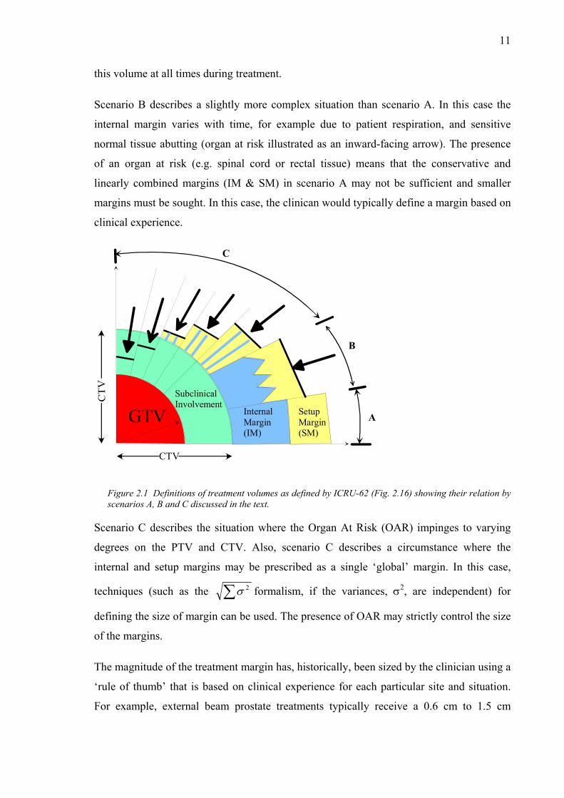
11
this volume at all times during treatment.
Scenario B describes a slightly more complex situation than scenario A. In this case the
internal margin varies with time, for example due to patient respiration, and sensitive
normal tissue abutting (organ at risk illustrated as an inward-facing arrow). The presence
of an organ at risk (e.g. spinal cord or rectal tissue) means that the conservative and
linearly combined margins (IM & SM) in scenario A may not be sufficient and smaller
margins must be sought. In this case, the clinican would typically define a margin based on
clinical experience.
CTV
C
B
ASetupMargin(SM)
Internal Margin(IM)
SubclinicalInvolvement
GTV
Figure 2.1 Definitions of treatment volumes as defined by ICRU-62 (Fig. 2.16) showing their relation by scenarios A, B and C discussed in the text.
Scenario C describes the situation where the Organ At Risk (OAR) impinges to varying
degrees on the PTV and CTV. Also, scenario C describes a circumstance where the
internal and setup margins may be prescribed as a single ‘global’ margin. In this case,
techniques (such as the ∑ 2σ formalism, if the variances, σ2, are independent) for
defining the size of margin can be used. The presence of OAR may strictly control the size
of the margins.
The magnitude of the treatment margin has, historically, been sized by the clinician using a
‘rule of thumb’ that is based on clinical experience for each particular site and situation.
For example, external beam prostate treatments typically receive a 0.6 cm to 1.5 cm
12
margin that may vary along each coordinate axis. The magnitude 0.6 cm to 1.5 cm was, in
some cases, used prior to measurements of the reproducibility of patient position and organ
mobility, but does coincide with current measurements from the literature. Statistically
oriented techniques utilizing in-house measurements of setup reproducibility and organ
mobility for sizing the margin have been proposed in the literature and are addressed below
(see §2.7.1).
Setup errors and organ motion aren’t the only factors causing uncertainty in the position of
the CTV, for example approximations of algorithms used in the treatment planning
software or simply inaccuracy in machine calibrations do exist. However, the predominant
(non-setup or organ motion) error is tumour delineation. That is, the volume of the tumour
delineated on the planning image may differ considerably depending on the clinicians, and
the methods and imaging modality used (Gademann 1996, Ketting et al 1997, Logue et al
1998, Rasch et al 1999, Valicenti et al 1999, Yamamoto et al 1999). Tumour boundaries
are not well defined. In particular, prostate GTVs defined using Magnetic Resonance
Imaging (MRI) have been found to be 30% smaller than those same tumours defined by
means of conventional Computed Tomography (CT) scans (Rasch et al 1999). Also
comparisons among clinicians show a factor of 1.8 variation in the CTV definitions for the
same tumour from the same set of images (Ketting et al 1997). Tumour delineation is
discussed in the ICRU-62 document, and should be considered in the definition of a PTV,
but is not explicitly described as belonging to either the IM or SM.
2.3. Comparison across studies
An attempt has been made in this section to average the mean and standard deviations
quoted in the literature across studies. In this case it is important to provide strict
definitions, as has been done below. However, the number of measurements adhering to
these definitions is greatly reduced from the total number of values quoted in the literature.
For example, consider the existing literature regarding the inter fraction movement of the
prostate (see table 2.1). Variables such as whether or not the rectum and/or bladder are full,
if an immobilisation device was used, the number of images (CT, simulation and portal)
per patient, the number of fields used, whether or not repositioning has been applied and
how, whether the patient was treated supine or prone, and even the stage (A, B, or C) of the

13
prostate cancer, can all affect the measurement.
Table 2.1 shows that for the case of inter fraction prostate motion, none of the reviewed
articles contain the same combination of parameters. Two broad methods of measuring the
position of the prostate were used in the reviewed studies. One method (M1) measured the
relative position of centre of mass of the prostate from bony anatomy. The other method
Table 2.1 Variation in parameters used for measurement of MODprostate.. Key: full (F) bladder/rectum, empty (E) bladder/rectum, rectum status Not Considered (NC), insufficient information provided (-). The numbers of images taken per patient refers to the number of images (CT, simulation and portals) used to derive their final measurement. Patients were treated in the supine (S) or prone (P) position, whether patient repositioning was done (yes, Y) or was not done (no, N), and the method used for the measurement (M1 or M2) from the text. In two studies the bladder/rectum content was increased with time (*), while in another study two time periods for voiding before treatment were examined (**).
Author
Year Rectum
Status
Bladder
Status
Patient
Immobil-
isation
images/
patient
Treated
position
Reposi-
tioning
Method
Ten Haken et al 1991 F* F* Y - S N M1,M2
Beard et al 1993 - - Y - S - M1
Schild et al 1993 F* F* N 3 S N M2
Balter et al 1995 - F N 4-8 - N M1
Crook et al 1995 - F N 6.5-7.0 S N M1,M2
Althof et al 1996 NC NC N 6 S - M2
Rudat et al 1996 NC NC N 4.5 S N M1
Melian et al 1997 F E** Y 4 P Y M1
Vigneault et al 1997 - - N N/A - N M2
Lattanzi et al 1998 F E Y 6-8 S Y M1
Roeske et al 1998 F - Y 5-8 S N M1

14
(M2) measured the relative position of markers (fiducial, radio opaque, or Foley catheter)
or prostate border (using CT images) relative to bony anatomy. Measurements of mean
prostate movement were all made relative to a ‘gold standard’ image that was taken either
during simulation or during the first fraction of treatment. Ten Haken et al (1991) and
Schild et al (1993) both describe the movement of the prostate as the rectum and bladder
were filled. Others describe the motion of the prostate during treatment not directly due to
bladder/rectum filling. (Beard et al 1993, Balter et al 1995, Crook et al 1995, Roeske et al
1995, Althof et al 1996, Rudat et al 1996, Melian et al 1997, Vigneault et al 1997, Lattanzi
et al 1998).
Variability in the reported parameters for other sites is also common - the prostate motion
is just one example. In this situation the most realistic approach is to represent the
published data in a uniform manner as outlined in the next section. The variability,
however, does highlight the conclusion that each institution should measure personalised
data for use with their clinical decision making.
2.4. Patient positioning (setup) errors
Fractionated external beam radiotherapy requires patients to be positioned for about 30
fractions of treatment, based on initial measurements done at planning. Thus, systematic
differences between the initial measurements and the desired positioning for a particular
patient may exist due to many factors including inaccurate alignment of positioning
devices and differences in cushioning capacity of couch material between CT and
treatment. Also random error will exist between the daily patient positions and the desired
patient position, due to factors such as the width of positioning laser beams and human
error. The patient positioning (or setup) errors then can be defined as consisting of
systematic and random components.
2.4.1. Defining Patient Positioning Errors
The treatment position deviation (TPD), ∆xi,j, is defined as the difference between the set-
up position described by the ith portal or CT image, from the setup position described at the
physical or digital simulation for the jth patient. These 'setup positions' are usually

15
measured using landmarks clearly visible on the Electronic Portal Imaging Device (EPID)
or portal film. The measurement includes components of both random and systematic
error. The jth patient may be described as having systematic error, jx∆ , defined as the
average TPD of that patient.
.1
j
n
ii
j n
xx
j
∑=
∆=∆ (2.1)
Equation 2.1 provides a calculation of systematic error in the x-direction only. Similar
measurements are made in the y- and z- directions and used with the calculations.
Generally the co ordinate system that is adopted is based on the patient co ordinate system
and defines x in the lateral direction, y is defined in the anterior-posterior direction and z is
defined in the superior-inferior direction. The positive and negative directions do differ in
the literature. In practise, the orientation and direction of x, y, z is based on the linear
accelerators software specifications and may differ between corporations. The distribution
of ∆ about the systematic error is defined as the random error, σix R,j, for the jth patient with
a variance defined as:
( )
.1
1
2
2, −
∆−∆=
∑=
j
n
iji
jR n
xxσ (2.2)
It is useful to define the mean treatment position deviation (MTPD), x , as the average of
TPD measurements over all N patients’ nj images within the study. Mathematically, the
MTPD is defined as:
.
1
1 1,
∑
∑∑
=
= =
∆= N
jj
N
j
n
iji
n
xx
j
(2.3)
If x is shown to be small, then the mean setup position over all patients is near the
position defined at simulation. It is important to represent the variation in the TPD using
the standard deviation, σT, of the data set because one set of data may vary more than other
sets. The variation in setup position will impact directly on the setup margin. The

16
magnitude of systematic error is important, but particularly if the systematic error is small,
the magnitude of the largest random shifts is important for setting a safe, conservative
setup margin. The setup error is generally written as x ± σT for a given group of patients.
For a population of patients the mean systematic error, Sx∆ , is defined as the average of
the systematic errors for each patient. The value of the mean systematic error will always
be close to that of the MTPD and identical to it if the number of portal images nj is equal
for all patients. Both the MTPD and the mean systematic error are important determinants
in locating setup technique errors at an institution. The systematic setup variation, ΣSE, is
defined from the standard deviation of the jx∆ data set over the j patients. The systematic
component then could be presented in a similar form to the setup error as Sx∆ ± ΣSE. The
mean random error for a population of patients is necessarily zero. The random setup
variation, σR, is calculated as the standard deviation of the set of data including all
( jji xx ∆−∆ , ) values. That is, the set of data including all patients’ TPDs subtracted from
that patient’s systematic setup error.
2.4.2. Magnitudes of positioning errors at various sites
Data for the typical magnitude of Setup Errors Averaged across Studies (SEAS) at a
variety of sites are presented in Table 2.2. The interested reader is directed to other review
articles on the topic, see Kutcher et al (1995).
Table 2.2 shows typical magnitudes of setup errors. The number of references attached to
each value indicates the number of studies that the corresponding value has been averaged
across, with the one exception. Bel et al (1996) provide results for prostate setup errors
from three institutions in the Netherlands. The statistics of the non-immobilised prostate
patient data is superior to those results with immobilised patients. A large number of
vacant cells appear indicating that no data was found for that entry or due to incongruent
presentation. Furthermore, it is noted that the prostate and pelvic regions are the most
extensively studied.
Generally, results for SEAS range from 0 mm to 3 mm (for both immobilised and non-
immobilised patients) across all sites. Immobilising the patient is shown to reduce SEAS,
but it has been noted in some studies that it is not beneficial. Results for σT across all sites
17
Table 2.2 The mean patient displacement averaged across studies (SEAS) and standard deviation σT (mm), with the systematic standard deviation ΣSE (mm) and the random standard deviation σ (mm).
Site Uncert SEAS(mm) σT (mm) ΣSE (mm) σ (mm)
Direct
ion
Immob No
Immob.
Immob No Immob. Immob No
Immob.
Immob No
Immob.
Prostate AP - 1.2 11,40,60,61 2.3 63 3.3 3,40,60,61,149 1.3 63 2.7 11,42,60,61 1.9 63 1.9 11,42,60,61
ML - 0.4, 11,42,60 2.7 63 3.0 3,40,60,149
, 1.9 63 2.4 11.40,60 2.0 63 2.0 11,60,61
SI - 0.9, 11,42,60 2.2 63 3.0 3,40,61,149, 1.4 63 1.9
11,40,60 1.7 63 1.7 11,60,61
Pelvis AP 1.2 71,155 0.5 57 5.3 74,156 3.6 57,156 - 8.1 171 0.7 155 2.5 173
ML 0.6 71,155 2.7 57,156 5.0 74,156 1.9 57,156 - 5.0 171 1.5 155 2.2 72,192
SI - 2.4 57,156 - 2.4 57, 156 - 6.7 171 - 2.9 72,192
Brain AP 0.66 57 N/A 2.24 57 N/A - N/A - N/A
ML 2.17 57 N/A 2.25 57 N/A - N/A - N/A
SI 0.67 57 N/A 2.58 57 N/A - N/A - N/A
Abdomen AP 0.7 155 - 4.9 155 - - - 1.8 155 -
ML 0.8 155 - 7.4 155 - - - 1.7 155 -
SI - - - - - - - N/A
H&N AP 1.1 11,70,193 N/A 2.3 70,193 N/A 1.6 11 N/A 1.7 11,193 N/A
ML 0.8 11 N/A N/A 1.5 11 N/A 1.8 11 N/A
SI 0.9 11,70,193 N/A 2.3 70,193 N/A 1.7 11 N/A 1.6 11,193 N/A
Chest AP 3.3 155 - 6.7 155 - - - 0.8 155 -
ML 1.3 155 - 7.1 155 - - - 2.1 155 -
SI - - - - - - - -
Lung AP - - - - - - - -
ML 2.3 193 - 0.8 193 - - - 2.5 193 -
SI 2.7 193 - 0.8 193 - - - 3.5 193
Rectum AP - 1.4 40 - 3.9 40 - 2.8 40 - 2.6 40
ML - 1.0 40 - 3.0 40 - 1.8 40 - 2.4 40 SI - 0.5 40 - 3.0 40 - 1.7 40 - 2.5 40
range from 1 mm to 7 mm, with results for the abdomen and chest providing the upper
range of 5 mm to 7 mm. Typical values for ΣSE and σR are in the same range as σT. Note
that the quoted values are one standard deviation, so for 90% confidence they should be

18
doubled.
It is important to note that the published results tend to be from advanced institutions and
may not indicate the variation applicable to the average busy department.
2.4.3. Patient Immobilisation
It is evident from table 2.2 that head and neck, brain, abdomen and lung treatments are
typically performed with immobilisation devices, while treatment at the pelvis is still in
debate. Verhey (1995) has published a review of patient immobilisation techniques by site.
Prostate immobilisation devices have yielded results that have been described as beneficial
(Soffen et al 1991, Rosenthal et al 1993) and not beneficial (Song et al 1996) for
improving the reproducibility of prostate treatment. Soffen et al (1991) reported a
reduction in the greatest ∆x measured during treatment by over 50% in each direction. The
value of x reduced from 8.0 mm to 3.3 mm. An increase in the percentage of exact
agreements with simulator increased from 22 % to 43 % because of the use of an alpha
cradle cast (extending from mid thigh to low thoracic area). This study used 20 port films
per patient. Bentel et al (1995) discovered that the number of isocentre shifts required to
achieve treatment position decreased by 20% for patients using custom made hemibody
foam cradles (formed around the supine patients back and down to their feet) compared to
non-immobilised patients, over a 7 week treatment course. Catton et al (1997) used a
treatment couch stiffened with polycarbonate inserts and a soft immobilisation device.
Values of x were decreased from 3.9 mm to 2.6 mm using this device and the percentage
of ∆x values greater than 5 mm was decreased from 17 % of setups to 8 % of setups.
Washington et al (1994) measured insignificant improvement in σT using immobilisation
devices against results without any immobilisation device (three tested). Among the
devices tested were the alpha cradle as used by Soffen et al (1991) and a styrofoam
immobiliser below the knees.
2.4.4. Pelvis
Table 2.2 lists ‘pelvic’ and ‘prostate’ as separate entries. This is because the literature
provides some studies that isolate measurements of the prostate, while others combine a
number of tumour sites in the pelvic region. The pelvic sites include genitourinary,

19
gynaecological, prostate, bladder, and rectal tumours.
Hanley et al (1995, 1997) have two separate sets of results listed in table 2.2. The former is
a retrospective study into the magnitude of setup errors for treatment of the prostate while
the latter is a study into the use of multiple projection port films. Results at that institution
have shown a reduction in systematic setup error because of the introduction of patient
repositioning when ∆x is measured to be greater than 2 mm. Greer et al (1998a) reported
that systematic setup errors in the AP direction were reduced for prostate from 3.7 mm to
1.2 mm, by adjusting the technique from setups with tattoos to using a table height method.
Bel et al (1995) also report highly accurate set-up results using a table height method,
although not for the pelvis.
Interestingly, Althof et al (1996) measured σT for both the bony anatomy and the prostate
(with I125 seeds). Measurements of the prostate set up error (included in table 2.2) showed
similar values as those for the bony anatomy with the largest difference being 0.2 mm. The
setup error for individual measurements (i.e. ∆x) ranged up to 9 mm (with no significant
differences between bony anatomy and prostate setup error).
Hanley et al (1995) measured an inherent uncertainty in the registration algorithm in portal
imaging software* (while imaging the prostate) of 0.6±0.5 mm in translation and 0.7±0.8°
in rotation within the 2D image plane. This uncertainty was increased to 2.3±1.0 mm and
1.2±1.1°, by applying a 2° out of plane rotation to the treatment planning computers 3D
dose matrix. Crook et al (1995) and Balter et al (1996) measured rotation around the AP
and ML axes using implanted radio opaque markers (3 per prostate). Crook et al (1995)
reported rotation of 1.63±1.55° around AP and 2.09±1.81° around ML. This rotation is
greater than that measured by Balter et al (1995) who quoted rotations of 0.2°, and 0.7°
about the AP and ML axes respectively.
Weber et al (2000) investigated the prone versus supine orientations for prostate treatment.
The random variations appeared similar for each patient orientation, but the prone
orientation provided larger systematic errors. Also, the prone position is associated with
higher dose to the rectum and/or bladder in over 30% of the patients.
* Varian PortalVision, software v.3.1.e., palo Alto, CA.

20
2.4.5. Brain
Gildersleve et al (1995) have published measurements of setup error (av. > 20 setups per
patient) involving stereotactic radiotherapy of the brain. In this study each of the 12
patients were immobilised using plastic (individually moulded) fixation shells for
simulation and treatment. Patients were positioned using marks on the cast with alignment
lasers for isocentric treatments. Values of x are about three times greater for the ML
direction, than for the AP and SI directions. Values of σ in each direction are similar at
between 2 mm and 3 mm. This suggests that the distribution was skewed because of a
systematic error (at this institution) in the ML direction. 13% of patients showed x to be
greater than 5 mm with none greater than 1 cm. A beam margin of 5 mm is suggested by
Gildersleve et al (1995). Rabinowitz et al (1985) measured σR equal to 3 mm for treatment
of the brain, with a positioning device.
2.4.6. Abdomen
Schewe et al (1996) measured set-up errors for a number of sites including the treatment of
abdominal cancers. Mean setup errors were measured as similar with standard deviations
greater in the ML direction than in the AP direction (see table 2.2). Rabinowitz et al (1985)
measured σR to equal 2.3 mm, for patients with abdominal cancer. These measurements are
similar in magnitude to those measuring abdominal motion (see table 2.4) suggesting that
much of the setup error may be due to abdominal movement. Interestingly, the setup errors
in the abdomen have been measured to be comparable to those at other sites within the
body, including the head and neck region.
2.4.7. Head and Neck
Magnitudes of SEAS for head and neck region (see table 2.2) show two predominant
trends including: 1) use of immobilisation devices eventuated in all presented cases, and 2)
highly accurate patient positioning across studies. Values of SEAS are typically around 1
mm with a value of σΤ equal to approximately 2 mm. The components of σ and ΣS appear
to be typically similar with values of each ranging from 1.5- 1.8 mm. Rabinowitz et al.
(1985) measured σ from a single head and neck patient to be 0.1 mm with an
immobilisation device. McParland et al (1993) measured field placement errors of the head
21
and neck region of immobilised patients to be 1.5±4.6 mm. Meertens et al (1990)
measured x between simulator and portal images with σT equal to 1.5 mm using an online
EPID system.
2.4.8. Breast
Westbrook et al (1991) measured setup errors for breast treatments. They measured the
movement of tattoos with a megavoltage imaging device and found that most (84%) of the
measurements fall within ±2 mm of the initial position. A large variety of patient and
breast sizes were evaluated with no substantial differences between patients based on
physical size. Other studies (Creutzberg et al 1993, van Thienoven et al 1991, Lirette et al
1995) generally measured larger positioning errors, with mean values of systematic
standard deviations ranging up to 4 mm, and maximum individual deviations ranging up to
around 15 mm for particular patients. A systematic error between the simulation patient
position and the reproduced patient position during the treatments was measured to be less
than 4 mm in each direction (Pradier et al 1999). Pradier et al (1999) suggest that for breast
treatments an immobilising device would improve the set-up reproducibility.
2.5. Organ motion
2.5.1. Defining organ motion
The motion of organs within the body can be broadly classified as moving randomly and/or
cyclically. For example, most organs in the pelvis are described as moving randomly
between fractions and organs in the abdomen are described as moving cyclically due to
breathing. These two types of organ motion need to be defined separately. The interested
reader is referred to a review article by Langen and Jones (2001).
Temporal prostate displacement is defined similarly to MTPD. The position of the organ
from bony landmarks is described at simulation, and then inter fraction deviation from this
position is measured during the treatment giving organ displacements. Alternatively, intra
fraction variations can be measured using movie clips obtained with imaging equipment.
All organ displacements from each patient are combined to form a data set from which a
mean organ displacement (MODorgan) is calculated with corresponding standard deviation
22
(σm,organ). The standard deviation of MOD is discussed more extensively in the literature
than the MOD. This is because the range of movement has been generally considered of
higher importance than the mean organ position. However, in recent years knowledge of
systematic error between planning CT images and the mean organ position during the
fractionated treatment has sparked increased interest in systematic organ motion error (van
Herk et al 1995). A novel investigation of the effect of (random inter patient) systematic
organ motion error on delivered dose is done below (refer to Chapter 4).
For those organs moving predominantly due to respiratory forces, for example abdominal
organs, most authors measure a total organ movement. The total organ movement is
defined as the total positional change of the organ from inspiration to exhalation.
Alternatively, for gated techniques that may include breathe holding, the reproducibility of
the organ position at breathe hold or at a particular part of the cycle (say, inspiration) is
required.
2.5.2. Magnitudes of organ motion
The Internal Planning Target Volume (IPTV) describes a volume to contain all movements
of the CTV relative to the bony anatomy. The CTV may be displaced between fractions
(inter fraction variation) or during the fraction (intra fraction variation). Inter fraction
variations occur due to various factors including, for example with prostate treatments, the
patient may void before some fractions, or the patient might not sit or lie on the treatment
couch in the same way for each fraction. Intra fraction variations may occur due to factors
including breathing, digestive processes or the pulsing of the heart or arteries. Obviously
the location of the tumour, the structure/function of nearby organs and the setup procedure
all have important influences on the motions, their magnitudes and the size of the IPTV to
include uncertainty. The literature suggests that many institutions are starting to utilise
values of the mean and standard deviations for inter fraction organ position and setup
uncertainty to prescribe a ‘global’ margin, and not two separate internal and setup margins
(as suggested by ICRU-62).
In the literature, organs in the pelvis (particularly the prostate) and abdomen are the most
thoroughly studied. Published movements of the prostate, abdominal organs and others are
summarised below. Techniques to reduce the organ movements are also explored. One of
the challenges in comparing the published literature is the variety in measurement

23
techniques between institutions. Therefore, further detail in some cases is provided
regarding the measurement techniques.
2.5.3. Prostate Motion
Measurements of prostate position have demonstrated movement of the organ due to
factors including partial rectum and bladder filling (inter fraction variations) and also due
to breathing (intra fraction variations). Studies have measured the prostate movements
specifically due to each of these factors and also neglecting these factors. Inter fraction
variations can be large in some circumstances. Therefore, an understanding of why the
prostate moves and how factors such as constant rectal volume affect prostate position can
be of great importance to accurate treatment field positioning.
Inter fraction variation is caused predominately by differences in rectal and bladder
volumes at each fraction (Melian et al 1997, Beard et al 1993). Recently, respiratory
induced prostate motion for patients who were positioned prone has been suggested as a
cause of non trivial movements (Malone et al 2000).
The measurement of prostate motion, neglecting the rectal and bladder volume provides
similar values of MODprostate and ΣOM (the standard deviation in MODprostate) in the
literature to those studies directly measuring the effects of these motions. Detailed
investigation of rectal and bladder effects is given in §2.5.3.2.
The MODprostate values presented in the literature range up to 6 mm, with σOM varying in
the range 1.3 mm to 4.5 mm. Typical values (MODASprostate) derived from measurements
of MODprostate, using prostate centre of mass or individual markers have been tabulated
below (table 2.3) with and without the patient being immobilised† during treatment. The
vacant column indicates no prostate motion information found (of suitable format) for non
immobilised patients in the literature. Movements tend to be greater in the AP direction
† Patient immobilisation devices refer to those devices that rigidly hold the patient in position for treatment.
They might be personalised. Other patient positioning devices such as neck or knee rolls, bars held by the
patient, or positioning lasers are not generally included in this description of patient immobilisation devices.

24
due to rectal filling, which might be intuitive from the geometry/position of the rectum.
Crook et al (1995) measured MODprostate with patient immobilisation using two methods.
Only the results from one of the methods (measuring positional change of the centre of
mass of three gold seeds) were consistent with our definitions and therefore included in
table 2.3. Results from the other study demonstrated that the prostate changes shape
between measurements.
Standard deviations in MODASprostate, ΣOM,prostate, for those patients treated with an
immobilisation device are typically reported to be similar to those measured without the
use of an immobilisation device. Several institutions have published improved results using
immobilisation devices. Standard deviations of MODASprostate with and without patient
immobilisation devices were presented in table 2.3. These values were comparable to those
directly measuring the effect of bladder/rectal filling on prostate positional change. For
example, Melian et al (1997) reported σOM,prostate values of 4.0 mm, 1.2 mm and 3.1mm, in
the anterior-posterior (AP), medio-lateral (ML) and superior-inferior (SI) directions,
respectively. Ten Haken et al (1991), measured σOM values of about 5 mm over the 31
patients in their Foley catheter study, and 2 mm for their CT study over 5 post implant
patients.
Table 2.3 Prostate position uncertainty due to the motion not directly attributed to bladder/rectum filling in the ant-post, medio-lateral and sup-inf directions. References are bracketed.
Site Uncertainty MODASprostate (mm) δprostate (mm)
Direction Immobilised Not Immobilised Immobilised Not Immobilised
Prostate AP 2.4 [31,93,147] - 3.2 [31,93,147] 3.2 [3,8,150]
ML 2.0 [31,93,147] - 1.0 [31,93,147] 1.5 [3,8,150]
SI 3.1 [31,147] - 4.1 [31,93,147] 2.7 [3,8,150]
MODASprostate and ΣOM,prostate in the ML direction is shown to be typically less than the
movement in the AP and SI directions, for both patients with and without immobilisation.
The superior portion of the prostate and the seminal vesicles tend to move more freely in

25
the anterior-posterior direction than the rest of the prostate (from a study with immobilised
patients, Melian et al 1997). Methods of measuring the position of the prostate from its
centre of mass assume that the prostate does not change shape, but the prostate has been
measured to deform (with dosimetric consequences) due to physiological effects (Forman
et al 1993) such as rectal and bladder filling. Therefore methods using markers or
measuring positional changes of the prostate borders may give a more representative
measurement of MODprostate.
2.5.3.1. Supine versus prone treatment positions
There may be advantages to treating patients in a prone rather than a supine position on the
treatment couch. The prostates of men positioned prone tends to shift anteriorly, due to
gravity, away from the rectum. Rectal filling has been correlated with prostate movements,
and thus less prostate motion is evidenced in the prone position. However, those prostates
of prone patients immobilised in thermoplastic shells can move substantially due to
respiration (Malone et al 2000). One study showed that twenty three percent (23%) of
patients treated prone and immobilised experienced intra fraction motions of greater than 4
mm. Calculations of rectal wall dose show reduced doses compared to patients treated
supine (Schild et al 1993, Zelefsky et al 1997). The average rectal dose (as a percentage of
the prescribed dose) was calculated as 64±1.3 % in the prone position and 72±1.1 % in the
supine position, despite the PTV’s being the same in both cases (Zelefsky et al 1997). No
significant difference in bladder wall dose was found. Melian et al (1997) noted that
treating patients in the prone position might increase bladder effects compared to the
supine position. It is also suggested that the prone position may not be suitable for those
patients who are obese or suffer significant orthopaedic/arthritic disease. In these cases the
supine position may be more practical and tolerable for the patient.
2.5.3.2. Bladder/rectum filling influence on prostate motion (MODprostate)
MODprostate values of 1 to 8 mm, due to rectal and bladder distension, were measured by
Ten Haken et al (1991) using the centre of mass of the prostate derived from CT images.
Greater movements of a Foley catheter balloon (i.e. 0 to 20 mm) due to rectal and bladder
distension were also measured. The effects of rectal wall and bladder movement have been
separately measured using CT images (Schild et al 1993). In this study, each border was
measured to move by different amounts. Filling of the bladder was found to cause posterior
26
movement of the prostate and seminal vesicles with maximum range of 0 to 8 mm and
maximum mean 2 mm (for posterior prostate margin). Rectal filling was found to cause
compression of the prostate and seminal vesicles in the anterior direction of maximum
range 0 to 17 mm and maximum mean 3 mm (for anterior seminal vesicles).
The effect of bladder filling can be inferred by comparing the MODprostate measured due to
bladder and rectum filling (Melian et al 1997), with the MODprostate calculated for patients
with full bladders (Crook et al 1995). Those MODprostate values derived separately for rectal
and bladder filling showed substantially smaller magnitudes than those reported with only
fixed bladder volumes. Despite this, the variation about the mean treatment positions (i.e.
σOM) were similar for both cases. The small values of MODprostate (less than 0.1 mm in each
direction) indicate that the distribution of prostate positions was centred at the position of
the prostate described at simulation. A systematic difference between the treatment
fractions and the single simulation image was present in the study using patients with full
bladders (Crook et al 1995). Constant volume of the rectum before and during treatment
appears to be a more important indicator than the bladder volume for prostate position
precision.
Indeed a time trend has been shown with movements of the prostate. The prostate tends to
move in a superior-posterior direction as the treatment proceeds. The position of the
prostate seems to be more constant near the end of the treatment (Lattanzi et al 1998). This
is thought to be due to incontinence induced by the irradiation of rectal tissue (Yeoh et al
1999). Forman et al (1993) suggest the presence of a systematic difference between the
mean position of the prostate measured during treatment and the mean position during
treatment plus the prostate position in the planning CT scan. Using CT scan images
Forman et al (1993) reported MODprostate/seminal vessicles measurements as 12 mm with ∆x
measurements ranging up to 37 mm during the treatment alone (i.e. disregarding the
treatment planning CT). Interestingly, when the treatment planning CT was included in the
calculations the mean shifted to 17 mm with ∆x values ranging up to 35 mm. This suggests
that the position of the prostate in the initial planning CT scan (typically used as the ‘gold
standard’ prostate position) was significantly different to the mean prostate position during
the treatment.
Chemotherapy combined with radiotherapy may affect the prostate volume and hence the
amount of movement possible within the pelvic chamber. The prostate volume has been

27
measured to decrease by 37% following radiotherapy and three monthly injections of
Lupron (Forman et al 1993, 1995). Radiation alone has been shown to decrease the volume
by an average of 14% after two weeks of fractionated radiotherapy (Roach et al 1997).
The stage of the tumour has been linked with the amount of inter fraction variation
measured (Ten Haken et al 1991). Patients treated with earlier stage disease appear to
exhibit larger movements (Ten Haken et al 1991, Crook et al 1995). Another study
however found no correlation between tumour stage and the inter fraction variation
(Melian et al 1997). Radical treatment of prostate cancer is usually only performed on
earlier stage tumours. Perhaps it may be inferred that the tumour stage (and
correspondingly increased size) causes the pelvis to restrict prostate movement for those at
later stages of the disease.
2.5.3.3. Strategies to account for prostate motion
A number of authors have made suggestions from the results of their measurements of
prostate motion. In particular Webb (1997) summarises four strategies. These may be
classified into those that accept organ motion and aim to account for the uncertainty with
the application of safety margins (Pickett et al 1993), and those that aim to monitor or
control motion (Balter et al 1993, Liebel et al 1994). Some strategies include;
Using a Foley catheter with rectal stent to keep the rectal volume constant (Ten Haken et al
1991).
Treat patients prone with full rectums and bladders (Schild et al 1993). The prostate
position then is not only more reproducible, but the inferred shift of the prostate is
advantageous to rectal sparing.
Image patients before each fraction and shift the linac isocentre accordingly. Daily CT
scans can be used to locate the prostate on each treatment day (Lattanzi et al 1998). The
bony anatomy is matched between the initial planning CT and the daily CT scans (called a
CT-CT fusion technique). The daily CT scans, amended planning and setup increased the
treatment time by 15 minutes for each patient. Also daily ultrasound has been suggested in
the literature to be a simple and reproducible technique (Lattanzi et al 1999). If the
isocentre is simply adjusted to the daily prostate centre of mass, deformation is obviously
being ignored, but can be included in the IM.

28
Non uniform (isotropic) margins should be used to compensate for prostate deformation
and the isotropic nature of the prostate motions (Pickett et al 1993).
These considerations are of great importance to IMRT and boost treatments (Deasy and
Cornett 1997) where the randomness of prostate motion is becoming a limiting factor to
dose escalation.
By accounting for prostate motion in the treatment planning software improvement has
been demonstrated in the calculated isodose distribution (Mageras et al 1994). Various
models of prostate motion exist with some assuming linear motion of the organ (Craig et al
1998), while others allow for separate motion in each direction of the entire surface or each
individual pixel (i.e. deformation)(Yan et al 1994, Fontenla et al 1997).
2.5.4. Abdominal Motion
While prostate motion is hypothesised to be caused by patient physiology, abdominal
motion is generally caused by respiration and is generally cyclic. During the past 20 years
methods to quantify and hence manage patient breathing and the corresponding movement
of abdominal organs have progressed forward with technological advances. Organ motion
within the abdominal cavity due to respiration has been quantified using computed
tomography (CT) (Balter et al 1996), magnetic resonance imaging (MRI) (Moerland et al
1994, Swartz et al 1994) and ultrasonography (US) (Oppelaar 1998, Davies et al 1994)
techniques.
The data available on radiotherapy aspects of respiratory induced organ motion are scarce
and more data is required.
2.5.4.1. Generalities
Measurements of MODabdominal under the same clinical conditions (e.g. breathing rate), of
the same organ, in a given direction and presented in the same form were not found in the
literature. Typical values (in a form similar to table 2.3) of MODabdominal could not be
derived for this reason. Instead a summary of results from the literature is shown in table
2.4.

29
Table 2.4 Summary of respiration-induced abdominal motion. The movement of the organ is the positional difference of the organ from inhalation to exhalation, unless otherwise stated. The details of the measurement may include a direction, breathing rate, alternate endpoint, or the condition of the organ at the time of measurement i.e. disease title.
Author Organ Movement (mm) Details
Balter (ref 7) Kidney (L) 18±6 AP, Normal Breathing (nb)
Balter (ref 7) Kidney (R) 18±6 AP, Normal Breathing
Swartz (ref 165) Kidney < 43 SI, Normal Breathing
Moerland (ref 126) Kidney (L) 2-24 Normal Breathing
Moerland (ref 126) Kidney (R) 4-35 Normal Breathing
Suramo (ref 165) Kidney (L) 19 (10-40) CC, Normal Breathing
Suramo (ref 165) Kidney (R ) 19 (10-40) CC, Normal Breathing
Kuhns (ref 87) Kidney 4.9±8.3 Breath hold @ inspiration
Kuhns (ref 87) Kidney 7.7±6.6 Breath hold @ expiration
Suramo (ref 165) Kidney (L) 41 (20-70) CC, forced respiration
Suramo (ref 165) Kidney (R ) 40 (20-70) CC, forced respiration
Ahmad (ref 2) Kidney (L) 1-32 Forced respiration
Ahmad (ref 2) Kidney (R) 3-21 Forced respiration
Moerland (ref 126) Kidney (L) 10-86 Forced respiration
Moerland (ref 126) Kidney (R) 10-66 Forced respiration
Kuhns (ref 87) Diaphragm 8.0±9.8 Btw exposures, nb
Davies (ref 34) Diaphragm 12±7 (7-28) SI, Normal Breathing
Balter (ref 7) Liver 17±5 AP, Normal Breathing
Suramo (ref 165) Liver 25 (10-40) Normal Breathing
Suramo (ref 165) Liver 55 (30-80) Forced respiration
Davies (ref 34) Liver 10±8 Quiet respiration
Suramo (ref 165) Pancreas 20 (10-30) Normal pancreas, nb
Suramo (ref 165) Pancreas 43 (20-80) Normal pancreas, forced
Kivisaari (ref 84) Pancreas 30±17 - 41±21 Normal pancreas
Kivisaari (ref 84) Pancreas 29±16 - 32±23 Pancreatis
Kivisaari (ref 84) Pancreas 14±6 - 25±1 Caput carcinoma
Using an ultra fast CT during normal breathing, Ross et al (1990) measured total
abdominal movement ranges up to 22 mm in the ML direction (with mean 6.1 mm) and up
to 15 mm in the AP direction (with mean 1.9 mm). Craniocaudal movements were greatest

30
near the diaphragm, while lateral movements were greatest near the heart or aorta.
Casamassima (1994) measured the kidney and liver to move by up to 3 cm during normal
respiration. Davies et al (1994) measured abdominal motion to be greatest in the
diaphragm, moderate for the kidneys and least for the liver, with motion of the diaphragm
and the liver predominantly in the SI direction. Tumours in the upper lobe and those
attached to the chest wall showed minimal movement.
The difficulties for comparison of results are the lack of measured directional information
for the movement, the different breathing rates requested of patients/volunteers in each
study, and the different endpoints of each measurement.
As expected, greater organ movement during forced respiration than during normal or
quiet respiration was reported at each site. Movement of organs has been shown to follow
complex paths when the patient breathes heavily. However, most studies considering
normal breathing show the variation in motion amplitude as being reproducible (with
standard deviations ranging from 6 to 8 mm for the kidneys, and up to 30 mm for other
abdominal organs).
2.5.4.2. Kidney Motion
Schwartz et al (1994) measured total kidney movement ranges up to 43 mm between
inhalation and exhalation, with the reproducibility (standard deviation of mean total
movement) at inhalation being 1.8 mm to 3.0 mm and 2.8 mm to 3.6 mm for exhalation,
using ultra fast MRI. No differences were found between the left and right kidney
movements, as measured by Balter et al (1996) or Suramo et al (1984) during normal
breathing. Moerland et al (1984) measured the range of displacements of the right kidney
to be greater than that of the left kidney during normal breathing. Both Moerland et al
(1984) and Ahmad et al (1997) found greater movements and movement variability of the
left kidney to the right kidney during forced respiration. The various borders of the kidney
were shown to vary by different amounts, with the internal border varying the least and the
inferior border varying the most.
2.5.4.3. Diaphragm Motion
Evaluation of diaphragm motion shown in table 2.4 demonstrates the measurement of
diaphragm movements using different endpoints. Kuhns et al (1979) measured the

31
variation in position between exposures, while Davies et al (1994) measured movement in
the SI direction during normal breathing at inhalation and exhalation. The results,
however, show similar values.
2.5.4.4. Pancreas Motion
Kivisaari et al (1982) measured total pancreas movement to be dependant on the condition
of the pancreas, with those considered normal or suffering pancreatitis being more mobile
than those suffering caput carcinoma. Pancreases with the former two conditions tended to
be most mobile at the tail and the body being least mobile. Those pancreases with caput
carcinoma tended to move most in the body and least in the tail of the pancreas. The
measurements of normal pancreas movement by Suramo et al (1984) show movements less
than those by Kivisaari et al (1982).
2.5.4.5. Breath Holding Techniques
Kuhns et al (1979) demonstrated the movement of the upper poles of the kidney for breath
holds to be 4.9±8.3 mm during inspiration and 7.7±6.6 mm during expiration. Suramo et al
(1984) devised a method, using a horizontal bar (able to move vertically) placed across the
patients’ chest, to reduce organ movement. In particular movements of the kidneys, liver,
and pancreas were decreased from 4 mm to 1 mm, 9 mm to 2 mm, and 6 mm to 1 mm,
respectively. Other attempts to improve reproducibility of lung volume for repeated breath
holds (during an imaging session) included providing the patient with an LED display
(Jones 1984) or a deflecting pointer (Frolich and Dohring 1985) to indicate chest height.
2.5.4.6. Advanced Techniques
Recent studies (Ohara et al 1989, Kubo and Hill 1996) suggest that the radiotherapy beam
may be gated by either a mechanical or physiological sensor resulting in “gated
radiotherapy”. This technique allows the patient to breathe freely during treatment without
the risk of compromising the accuracy of the dose delivery. Another two techniques which
utilise gated methods are Predictive Respiratory Gating (Richie et al 1994) for imaging and
Active Breathing Control (Wong et al 1997) for radiotherapy. The gating mechanisms are
currently standard on some commercial linear accelerators.
Predictive Respiratory Gating uses an algorithm that predicts the time taken to restart
inspiration after end of expiration and then aligns the CT acquisition accordingly (without

32
assuming periodic motion). Whilst Active Breathing Control differs by additionally
involving a device that feeds the patient air, and thus controls their breathing cycle. At a
predetermined time the apparatus cuts the air supply and holds the lung volume constant
while a periodic dose is given. Clinical studies (Wong et al 1997) have shown that patients
can comfortably hold their breath for around 15 seconds at the end of expiration and from
25 to 50 seconds at the end of inspiration. During this time period the lung volume changes
by less than 5%.
2.5.4.7. Patient Orientation during treatment
Willet et al (1987) found that Hodgkin’s disease patients treated in the standing position
had a lower ratio of the mediostinal mass to the inter thoracic diameter than those patients
treated supine and prone, during quiet respiration. For heavy breathing no appreciable
difference occurred between the patient positions. Harauz and Bronskill (1979) found no
appreciable improvement (regarding liver motion) in positioning the patient supine
compared to having them stand. The respiratory amplitude decreased from 14 mm to 12
mm.
For a given patient, the movement of abdominal organs deduced during the initial imaging
session tends to reflect the movement through the treatment course (Opelaarr 1999).
Organs within the abdomen are physically fixed in position and respiration may cause the
organs to move substantially. Abdominal motion tends to reflect the distance of the organ
from the diaphragm, and might represent the respiratory frequency of the patient. Gated
and breathing control techniques match these circumstances.
Abdominal organ position distributions have been shown to be reproducible across patients
after the initial sizes and locations have been measured. This has suggested the possibility
of modelling organ movement by applying the fixed variation to the personalised initial
organ position image (Yan et al 1997).
2.6. Patient Repositioning strategies
Patient repositioning using portal images can dramatically reduce systematic set-up errors
(Shalev and Glutchev 1994, Yan et al 1994). The megavoltage or kilovoltage (Pisani et al
2000) portal image is compared to a benchmark simulation image and specialised

33
computer software is used to detect shifts in the bony anatomy between the two images. If
a shift is detected, and it is larger than a prescribed action level, a decision can be made
(off line) for the patient to be shifted before the next fraction. Alternatively, the decision
can be made in real time and the shift, if any, can be made (on line) for the current
treatment fraction. The on line procedure adds 3-10 minutes to each fraction (Stroom et al
2000, Pisani et al 2000).
Balter et al (1993) modelled repositioning patients on-line. They initially measured that 17
out of 27 port films demonstrated shifts (∆x) greater than or equal to 1 cm. Replacing those
measured values that were greater than 1 cm with higher accuracy random error data
(ranging from 1 mm to 4 mm), the minimum tumour coverage with reduced field margin
compared well to that of normal treatment, illustrating that repositioning the patient would
be beneficial. Moreover, reducing the systematic error using on-line repositioning is
thought to justify the reduction of margins 1 cm to 0.5 cm for gynaecologic tumours
(Stroom et al 2000).
Many criteria for prescribing a suitable action level have been described in the literature
(Yan et al 1994). Bel et al (1996) suggest a two stage, shrinking action level (SAL)
protocol for prostate treatment (known as the Amsterdam method). The first stage involves
measuring the ∆x over the first few fractions and comparing the measured values against
the diminishing action level calculated as τ/µ, where τ is the initial action level and, µ is
the measurement number. A minimum of two measurements are taken and if the measured
value of ∆x is greater than the action level then the isocentre is shifted in the next fraction
by the cumulative x in each direction and stage 1 is restarted. The initial parameters (τ and
µ max, the number of consecutive treatment sessions featuring portal image acquisition)‡ are
calculated using derived (patient specific) values of σT in a computer simulation. When the
required accuracy is achieved the second stage begins. The second stage is based on a
weekly check of the setup accuracy. This method ignores rotations as they have been
measured in the literature and were shown to be small for prostate treatments (van Herk et
al 1995, Bijhold et al 1992). The method also assumes that the σR is the same for each
patient (Bijhold et al 1992). This procedure improved the percentage of ∆x measurements
‡ Typical values for τ, µ max range from 6 mm to10 mm, and 2 to 4, respectively.

34
that were greater than 5 mm from as high as 42.7% to less than 1%, requiring about 12
measurements per patient. Other techniques have been suggested to reduce the average
number of measurements per patient using a No Action Level (NAL) protocol (de Boer et
al 2001). The NAL protocol measures patient positioning over a specified number of
fractions before the single repositioning per patient per treatment and is similar to the
Newcastle method described below.
Following diagnosis of a discrepancy the Amsterdam method prescribes repositioning of
the patient by the whole measured shift despite this measured shift containing components
of random and systematic error. Pouliot and Lirette (1996) suggest that only the systematic
component of the measured discrepancy should be included in the repositioning of the
patient following the diagnosis of an error. They proposed using the full maximum
likelihood theory (FML) to derive that the magnitude of the required shift is the measured
discrepancy multiplied by the FML factor. The FML factor is calculated from the standard
deviations of the systematic error SDsys and random error SDrand, as FML = SDsys2 / (SDsys
2
+ SDrand2). This procedure is optimal when the component of random error is large, and the
method seeks to prevent over corrections.
The flow of operation suggested by Bel et al (1996) and by Pouliot and Lirette (1996)
assume that the measured discrepancies in each direction are independent and a history of
errors associated with that site and procedure are available. See et al (2000) test a further
method (the Newcastle method) that does not assume the discrepancies are independent
and builds case histories for each patient as they are treated. The Newcastle method
schedules the patient treatment into two sections, these are; diagnosis during the first week
and intervention during the remaining weeks. No corrections are made during the first
week, but portal images are acquired and the 3D discrepancies are detected. Hotelling’s T2
statistics are used to prescribe the action level for that patient and to provide useful
statistics. The action level is not simply three single direction scalars along each coordinate
axis, but plots of the measurements including a multivariate analysis to detail whether the
movements in each direction are independent. The method is not based on population
statistics and although the derivation of individual patient action levels is advantageous the
number of portal images required and the associated workload could limit the clinical
usefulness.

35
2.7. Contemporary suggestions for treatment planning
The provision of a margin between the CTV and the PTV based on a ‘rule of thumb’ is not
the optimal technique to account for targeting uncertainty. This is because the rule of
thumb may offer no patient specificity, no scientific basis and may not consider the
directional dependence of the errors. Statistical dose based methods have been suggested in
the literature to size the CTV-PTV margin and also to adaptively conforms dose to the
tumour while the treatment progresses and individual data are generated (Craig et al 2001).
It should be noted that many radiotherapy clinics are not yet utilising any of these
techniques.
2.7.1. Statistics based treatment margins
The sizing of a margin between the CTV and PTV is a balance between the targeting
accuracy and dose constraints on tumour and normal tissue. The margin should be
sufficient to account for all geometric errors such that the CTV accumulates no less than,
say, 95% of the prescribed dose. Various factors have been included in the statistical
techniques for manufacturing a suitable margin.
One of the original suggestions for sizing the margin came from Goitein (1985) who
conjectured that the CTV-PTV margin, H, should equal 1.5 multiplied by the standard
deviation of combined target/patient motion. At this stage of history, the positioning of
dose in space was not as precise as it became during the 1990’s. The basic premise at this
stage was, and still is in a large number of centres, the ‘global’ margin identified in §2.1.
The global method calculates a margin from the root of the measured variances of patient
positioning error plus organ motion assuming that the two uncertainties are independent:
H = NSD(Σ2 + σ2random)½ (2.4)
The technique then uses population statistics, and the margin is based on certain numbers
of standard deviations, NSD, providing a certain probability of PTV coverage. For example
2 standard deviations refers to a 90% probability of PTV coverage.
There are other further advanced techniques that account for the geometry of the tumour,
the systematic and random components of setup error and the beam geometry. The
geometry of the tumour can be incorporated to allow for the areas of tumour near beam
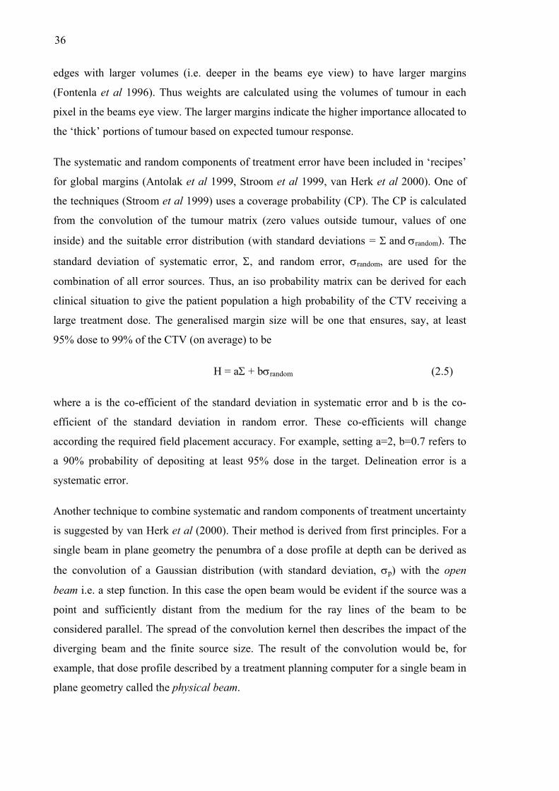
36
edges with larger volumes (i.e. deeper in the beams eye view) to have larger margins
(Fontenla et al 1996). Thus weights are calculated using the volumes of tumour in each
pixel in the beams eye view. The larger margins indicate the higher importance allocated to
the ‘thick’ portions of tumour based on expected tumour response.
The systematic and random components of treatment error have been included in ‘recipes’
for global margins (Antolak et al 1999, Stroom et al 1999, van Herk et al 2000). One of
the techniques (Stroom et al 1999) uses a coverage probability (CP). The CP is calculated
from the convolution of the tumour matrix (zero values outside tumour, values of one
inside) and the suitable error distribution (with standard deviations = Σ and σrandom). The
standard deviation of systematic error, Σ, and random error, σrandom, are used for the
combination of all error sources. Thus, an iso probability matrix can be derived for each
clinical situation to give the patient population a high probability of the CTV receiving a
large treatment dose. The generalised margin size will be one that ensures, say, at least
95% dose to 99% of the CTV (on average) to be
H = aΣ + bσrandom (2.5)
where a is the co-efficient of the standard deviation in systematic error and b is the co-
efficient of the standard deviation in random error. These co-efficients will change
according the required field placement accuracy. For example, setting a=2, b=0.7 refers to
a 90% probability of depositing at least 95% dose in the target. Delineation error is a
systematic error.
Another technique to combine systematic and random components of treatment uncertainty
is suggested by van Herk et al (2000). Their method is derived from first principles. For a
single beam in plane geometry the penumbra of a dose profile at depth can be derived as
the convolution of a Gaussian distribution (with standard deviation, σp) with the open
beam i.e. a step function. In this case the open beam would be evident if the source was a
point and sufficiently distant from the medium for the ray lines of the beam to be
considered parallel. The spread of the convolution kernel then describes the impact of the
diverging beam and the finite source size. The result of the convolution would be, for
example, that dose profile described by a treatment planning computer for a single beam in
plane geometry called the physical beam.

37
To investigate the typical magnitude of the σp parameter a simple computer program was
written. The program reads an input dose profile and then separately calculates the
convolution of a Gaussian function with a step function for comparison. The input dose
profile is visually compared to the result of the convolution with various σp values. Using
the input dose profile from a 10x10 cm2 beam of 6 MV photons, the value of σp was
calculated to be 3.2 ± 1.0 mm. Using the oblique and lateral profiles through a four field
box technique, the fitted values of σp were 6 ± 1 mm (with lower dose cut off 5 Gy) and 5
± 1 mm (with lower dose cut off 35 Gy), respectively. The literature provides the value 3.4
mm as a typical magnitude (van Herk, 2000).
For a single beam multi fraction treatment the random positioning uncertainty experienced
for each fraction of treatment can be characterised by Gaussian σrandom, and will lead to a
dose profile given as the convolution of the physical beam with the random error. If we
wish to use the geometrical beam, then we must perform a convolution with the combined
error (given as σ2 = (σp2 + σrandom
2)1/2 ). Thus, including the random component of error, to
cover the CTV with the PTV from the 90% dose point on the penumbra a margin of 1.28(σ
– σp) should be added. To accommodate systematic error, such as delineation error at the
treatment preparation stage, a margin of 2.5Σ is derived to succeed for 90% of patients.
Therefore, to include the CTV within the PTV for 90% of patients to 90% of prescription
dose the margin required is
H = 2.5Σ + 1.28(σ-σp). (2.6)
For higher confidence that the CTV will be enclosed within the PTV for all fractions, other
coefficients can be used. For example, for 95% of prescription dose the coefficient of
random error is 1.64 and for 95% of patients the coefficient of systematic error is 2.79.
Another technique using the combined standard deviation of random and systematic error
(where Σtotal is the root of the systematic and random variances added in quadrature)
provides an alternative to the requirement of enclosing a point on the surface of the CTV
inside the PTV. Antolak and Rosen (1999) have shown the theoretical probabilities of
movement from a point by a certain distance in 1D, 2D, and 3D space. Most relevant is the
3D case, where they use the integral form of the Maxwell equation to express that the
probability of finding an object within the sphere of radius R is (Antolak et al 1998):
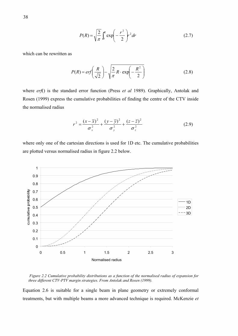
38
∫
−=
RdrrrRP
0
22
2exp2)(
π (2.7)
which can be rewritten as
−⋅−
=
2exp2
2)(
2RRRerfRPπ
(2.8)
where erf() is the standard error function (Press et al 1989). Graphically, Antolak and
Rosen (1999) express the cumulative probabilities of finding the centre of the CTV inside
the normalised radius
2
2
2
2
2
22 )()()(
zyx
zzyyxxrσσσ−
+−
+−
= (2.9)
where only one of the cartesian directions is used for 1D etc. The cumulative probabilities
are plotted versus normalised radius in figure 2.2 below.
0
0.1
0.2
0.3
0.4
0.5
0.6
0.7
0.8
0.9
1
0 0.5 1 1.5 2 2.5 3
Normalised radius
1D2D3D
Figure 2.2 Cumulative probability distributions as a function of the normalised radius of expansion for three different CTV-PTV margin strategies. From Antolak and Rosen (1999).
Equation 2.6 is suitable for a single beam in plane geometry or extremely conformal
treatments, but with multiple beams a more advanced technique is required. McKenzie et

39
al (2000) derived an alternate co-efficient, η, for the random component of error depending
on the number of beams used (up to 6 beams) and whether the beams are parallel and
opposed or not parallel and opposed. The margin is then
H = 2.5Σ + η(σ-σp), (2.10)
where η ranges from 1.64 for a single beam to 0.52 in the transverse plane with 6 beams.
Generally, the values of η are greater than one in the transverse and cranio-caudal
directions assuming that the patient is treated parallel to the linear accelerator gantry.
The techniques for margin calculation discussed thus far have been predominately
theoretical and dose-based. In practise the margin calculated with one of these margin
recipes may include a portion of a sensitive normal structure and in that case other factors
need to be considered. Other factors may include DVHs, or biological indices such as the
normal tissue complication probability. In essence though, these other factors do refer to
clinician input directed towards either changing the margin in some way or progress
without any changes. Recently, van Herk (2001) has calculated a margin rule that
considers the tumour control probability. In that work, decreasing the existing margin by 3
mm was calculated to reduce the probability of tumour control by 1%.
Mageras et al (1999) have developed a technique to include population based
measurements of patient positioning and organ motion uncertainty into a prescribed dose
volume (PDV). The PDV is used to set margins by weighting the importance each region
of interest and allocating limits of dose.
In general the margin ‘recipes’ to date have separated uncertainty into systematic and
random components. This does not conform to the IM and SM suggested in ICRU-62
(1999). The ICRU-62 document is still relatively new (at the time of writing) and only time
will tell if it’s suggestions are put into practice.
2.7.2. Adaptive radiation therapy
Adaptive radiation therapy involves constantly optimising the planning of a treatment as it
proceeds according to the accumulating knowledge of each treatment. Thus as portal
images are obtained and the distributions of set-up and organ positions become more
reliable, the treatment margins can be adjusted accordingly. This broad system of treatment

40
was proposed by Yan et al (1997a) and has been developed further in recent years (Yan et
al 1999, Yan et al 2000, Yan and Lockman 2001). The latest system involves kilovoltage
imaging attached to the linear accelerator so that organ motion and setup errors can be
reasonably eliminated.
2.7.3. Monte Carlo techniques
Killoran et al (1997) suggest a Monte Carlo technique that iteratively samples from
population distributions of setup errors and organ motion. The result is a probability of
prescription dose curve, which directly relates the margin size with the probability that the
CTV will accumulate the prescription dose. This method allows patient specific
distributions for each known uncertainty to be included, but computation times are high.
Mageras et al (1996) have devised a method to include a population of serial CT images
with a planning CT image set to provide information on the potential extent of prostate
movement. The region of interest data (reflecting outlined target and non-target organs)
from the population of serial images is included on a current patients CT image set. The
statistics of the past organ positions are used to calculate a confidence limited dose volume
histogram (CL-DVH). The CL-DVH offers the dose deposited to incremental volumes of
the specified region of interest tissue, allowing for possible organ movement, within
specified confidence limits. Thus, potential organ movements are predicted and included
into a DVH. The DVH itself includes no spatial information and therefore the magnitudes
of organ motion in each direction may not be easily interpreted. The method also ignores
systematic organ shifts from planning to treatment by treating all images with equal
weight.
In this thesis, a Monte Carlo code is developed that calculates the standard deviation in
deposited dose based on the statistics of the organ motion. With this tool, the regions on
the planning CT image that attract the most uncertainty in deposited dose are elucidated.
The MC technique presented in §4.3 allows inclusion of single or multiple CT image sets,
and details the magnitude of dose advantage from multiple CT scans and the size of the
potential regions of regret from the normal practise of single planning CT scans.

41
2.7.4. Convolution techniques
The convolution integral has been used previously for reducing statistical noise in
electrical circuit applications. More recently, in radiotherapy, the convolution integral has
been used to model the interaction of high energy photon beams with matter and used for
calculating dose in treatment planning systems (Mackie et al 1984). However, the
application of the convolution integral has also been utilised for calculating the effect of
treatment uncertainties (Leong, 1987). The general form of the convolution integral is
∫ ′⋅′−=′ xdxgxxfxf )()()( (2.11)
where f is the planned dose distribution, g is a probability distribution function (PDF)
describing the treatment uncertainty and f′(x) is the mean delivered dose distribution. Since
the method uses the precalculated dose distribution from the planning system with an
existing PDF, and involves one simple calculation, this technique is easily implemented
into a treatment planning system. Once the delivered dose distribution has been calculated
the associated DVH can be created and compared with both the original plan DVH and
rival plan DVHs (Keall et al 1999). Moreover, the convolution technique has been
extended from calculating only the mean delivered dose to calculating the standard
deviation in mean dose (Zavgorodni 1997, Lujan et al 1999). Bel et al (1996) used
deconvolution to calculate CTV→PTV margins.
However, the weakness of the convolution technique is the assumptions that it is based on.
These assumptions include (but are not limited to) the organ not deforming during
treatment, uncertainty obeying the PDF through out each patients’ treatment, and the lack
of heterogeneities. Obviously, some disease sites will better conform to these assumptions
than others. The prostate, as has been detailed previously, does conform well to the
assumptions of the convolution method and is a candidate for accurate use of the
technique. The prostate is located in the rather homogeneous bony pelvis, deforms only
moderately with physiological function, and shows reasonably small variations from the
PDF during a 5 week course of radiotherapy.
There are, however, still areas that need to be improved upon with the convolution
technique. In this thesis (§4.4) the technique is extended to predict the effect of single and
multiple planning CT images on the precision of dose delivery. As explained previously,

42
the systematic error of prostate location is a discrepancy between the planning CT image(s)
and those taken during treatment are substantial and should be included extrinsically in the
planning process. Further detail is given in Chapter 4.
2.8. Summary
This chapter has demonstrated the significance and importance of considering the
inevitable uncertainty during the planning and delivery of a radiotherapy treatment. Across
all sites, the inclusion of knowledge regarding the magnitudes and characteristics of the
errors should be considered. Combined with techniques to control the magnitude of errors,
careful efforts need to be employed to account for them as well. The best opportunity to
account for uncertainty is in the planning process, using methods that reflect the statistical
nature of many of the errors.
The prostate has been illustrated to move up to 2 cm interfraction due to rectal, and to a
lesser extent, bowel distension (Ten Haken et al 1991). Following the suggestions of the
ICRU reports, combined with statistical dose based techniques, suitable CTV→PTV
margins can be calculated. But, a large unpredicted movement is always possible, as is a
patient-specific trend. Repositioning the patient is not trivial because the prostate is not
visible in portal images. Other imaging techniques, such as kilovoltage or CT have been
suggested in the literature. However these techniques have not been shown to be efficient
or integrated into commercial treatment planning software.
Clearly, the prediction of potential organ movement and patient position is the best option.
Accordingly, a number of considerations are explored in this thesis deriving from
knowledge of the prostate motion and patient positioning characteristics. One such
characteristic is the potential systematic prostate position error between planning and
treatment. The ramifications of not considering this error when managing errors during
treatment delivery are explored in Chapter 4 using both convolution and MC techniques.
The impact of the errors at planning and treatment on the tumour and normal tissue
response are calculated with biological models in Chapter 6. Possible techniques for better
displaying the potential error are explored in Chapter 7.

43
Chapter 3
Review of radiobiological models
3.1. Introduction
This chapter introduces the concepts that are important for investigation of the
radiobiological impact of the potential errors in the dose delivered to the tumour site and
surrounding tissue investigated later in this thesis.
The chapter contains a description of the current radiobiological models used within
radiotherapy and discussion of their relative merits. The relevant concepts outlined include
the Biologically Effective Dose (BED), Standard Equivalent Dose (SED), Equivalent
Uniform Dose (EUD), Tumour Control Probability (TCP), Normal Tissue Complication
Probability (NTCP), and Uncomplicated Tumour Control Probability (UTCP).
The calculation of TCP for prostate carcinoma is outlined in detail following the general
discussion of TCP. A number of radiobiological aspects such as the currently considered
fractionation regime (from the literature) for prostate carcinoma will be reviewed. The
feasibility of using the calculated TCP for prostate cancer is discussed. With NTCP, the
particular case of late rectal complications is outlined in further detail to highlight the
growing knowledge base surrounding the choice of parameter values and their meaning.

44
3.2. Biological Models
Biological models can be grouped as being either empirically or theoretically based. The
empirical models derive from fitting curves to actual clinical data. Strictly, these models
are then only valid for situations described by the original clinical data. Alternatively,
theoretical models are based on some insight into radiation interaction with cells and DNA
and the processes involved. These models require the theory for each process. It is
important for the user of such models to take into account the limitations in identifying and
theorising about each of the processes.
An important proviso when using the radiobiological tools derived from these models is to
remember that they have a limited application, are based on incomplete laboratory data,
and that they should be superseded by clinical experience. Box puts this in perspective
when he writes “All models are wrong, but some are useful!” (Box, 1984).
3.2.1. Empirical (Probit and Logit) Models
The two most common empirical models are the Probit and Logit models. The Probit
model (Lyman, 1985) was derived from tolerance dose data for various percentage
volumes irradiated across a variety of organs (and is plotted in figure 3.1). The Probit
model can be described by the probability of effect following radiation dose, D using:
−−=
50
1121)(
DDerfDP probit γπ
(3.1)
where erf() is an error function, γ is the slope of the dose response curve at 50% response,
and D50 is the dose to cause a given effect (or endpoint) in 50% of the population. For
tumours the desired effect is total eradication of all clonogenic cells, while for normal
tissue, the effect could be anything from a range of undesired complications, such as skin
reddening (erythema).
The error function used in equation 3.1 is a form of the gamma function expressed as:
( ) ∫ −=x
t dtexerf0
22π
(3.2)

45
The Logit model was proposed by Schulthiess et al. (1983) and is plotted in figure 3.1. The
logit model states that for dose D, the probability of effect will be;
14501)(
−
+=
γ
DD
DP Logit
(3.3)
where γ is (again) the gradient of the dose response function at D50. Both the Logit and
Probit models have been fitted to normal tissue dose-volume response data.
0
0.1
0.2
0.3
0.4
0.5
40 45 50 55 60
Dose (Gy)
ProbitLogit
Figure 3.1 Plots of Probability of effect following single fraction irradiation to dose, as calculated with the Probit model (solid curve) and Logit model (dashed).
3.2.2. Theoretical (Poisson/Linear Quadratic) Model
The Poisson model is the most commonly used in radiotherapy, particularly in the linear-
quadratic (LQ) form. Using Poisson statistics, the probability of n surviving cells where the
expected value is Ns may be written
( )
!nNenP
ns
Ns−
= (3.4)
For tumour control the number of clonogens remaining will be zero, setting n=0, the
tumour control probability (TCP) is;

46
s
sNs
N
eNeTCP −−
==!0
0
(3.5)
The linear quadratic model provides an expression for the surviving fraction, S, of
mammalian cells after low LET irradiation.
The theory behind the shape of the shouldered mammalian cell survival curve relates the
linear and quadratic terms in dose to cell kill. The interaction of ionising radiation with the
cell DNA causes strand breaks that lead to cell necrosis or apoptosis. Single strand breaks
can be easily repaired, while double strand breaks are less likely to be repaired and more
likely to cause cell death. The number of hits that are required to kill the cell i.e. single hit
or multiple hits can be linked to the probability of single or double strand breaks. The
linear coefficient in dose, α, describes the shoulder resulting from cell death dominated by
single hit kills, while the quadratic term in dose, β, describes cell death requiring multiple
interactions. This allows for cell repair to occur and is the principle allowing fractionation.
For high LET particles like alpha particles the fraction of single hit deaths is higher than
for low LET radiation such as gamma radiation so that an alpha particle cell survival curve
will show essentially no shoulder.
Considering a tumour originally containing N0 tumour cells irradiated to total dose, D, then
the surviving fraction (Ns/N0) is given by (Fowler, 1989)
.)(
2
0
DDs eNNDS −−== βα
(3.6)
The cell sensitivity for a particular tumour or tissue type is indicated by the constants, α
and β. These are illustrated in figure 3.2 for two types of tissue; early and late responding
tissues. Typically early responding tissues characterise tumour, while the late responding
tissues will typically characterise normal tissue (or side effects). The ratio of α/β will also
provide valuable information on the tissue response to radiation. With tumours, the α/β
ratio generally has the value ~10, while for normal tissue the α/β ratio will have the value
~3. Therefore, the β term is sometimes dropped when relating to tumour control. There is
naturally a range of possible α and β values across tissue and tumour types, and these rules
will not always hold.

47
From equation 3.5 we may insert Ns(=N0S) into equation 3.4, which simplifies to give
[ ],exp)( )( dDtLQ eVDP βαρ +−⋅⋅−= (3.7)
where the product of the clonogen density, ρ (cm-3) and the tumour volume, Vt (cm3)
calculates the initial number of clonogens, N0, and the total dose, D=nd, is the number of
fractions, n, multiplied by the dose per fraction, d.
1.0E-10
1.0E-09
1.0E-08
1.0E-07
1.0E-06
1.0E-05
1.0E-04
1.0E-03
1.0E-02
1.0E-01
1.0E+00
0 2 4 6 8 10 12 14 16 18 20
Dose (Gy)
Late responding
Early responding
Figure 3.2 Surviving fraction versus dose for early responding tumour tissue and late responding normal tissue. Tumour is characterised by α = 0.35 Gy-1 and α/β = 10, while normal tissue is characterised by α = 0.15 Gy-1 and α/β = 3 (from Metcalfe et al. 1997).
For rapidly proliferating tumours, such as those of the head and neck, an extension to the
conventional LQ model has been proposed (Lee et al 1995). The survival fraction will then
be calculated as;
−++−= )(2ln)(exp k
pot
TTT
dndS βα (3.8)
where Tpot is the potential doubling time, T is the total time of treatment and , Tk, is the
kick-off time. The potential doubling time is the time taken for the number of clonogens to
double, and the kick-off time is the time taken for the irradiation to induce an increased
proliferation rate.

48
3.2.3. Hyper sensitivity of tumour/normal tissue at low doses
Recently, a hypersensitivity to doses lower than ~0.5 Gy per fraction has been shown for
26 human cell lines including both tumour and normal tissue (Joiner et al 2001). The
hypersensitive response occurs maximally at doses around 0.5 Gy as shown in figure 3.3.
The LQ model has been shown to significantly underestimate response in the dose range
up to 1 Gy. However, two models have been suggested as extensions of the standard LQ
model (refer to equation 3.6) to include the low dose hypersensitivity. The two models are
the two population model and the induced repair (IR) model.
The two population model states that the increased sensitivity is due to the more
radiosensitive cells in the G0 phase of the cell cycle being predominately killed. However,
this model has been subsequently revoked due to the magnitude of the hyper sensitivity
being larger than would be predicted from merely cell cycle differences. Additional
evidence for rebuttal of this model came from an experiment where cells were repeatedly
irradiated in the dark where the cell cycle is arrested (Howard and Cowie, 1978). The cells
still showed the hypersensitive response.
Figure 3.3 Survival fraction versus dose for T98G human glioma ceexperimental data points, the dashed curve is the LQ model predic
α
lls. The dots with error bars are the tion, and the solid curve is the IR
49
model prediction. From Joiner et al. (2001).
The IR model is based on a threshold dose. Prior to this threshold dose (generally
following up to ~0.5 Gy) the tissue is hypersensitive, but when the dose has exceeded the
threshold repair mechanisms are induced in the tissue and the effective cell sensitivity
reduces greatly. The IR model can be expressed in terms of effect on the surviving fraction
as (Lambin et al 1994):
−
−+−= − 2)1(1exp ddeS cdds β
ααα , (3.9)
where αs is the larger tissue sensitivity at very low doses; and dc is a constant which
describes the dose range over which induction of repair occurs.
3.2.4. Biological Effective Dose
Until Barensden introduced the concept of Extrapolated Response Dose (ERD) in 1982
(later renamed Biological Effective Dose (BED) by Fowler) radiobiology was not widely
used in radiotherapy. The BED provides a simple method of including the biological
response of tissue from fractionation and total dose. The Biological Effective Dose is
defined as the dose delivered with a fractionation schedule that delivers 0 Gy fractions;
D(α + βd) = BED(α + β×0) (3.10)
+=
βαdDBED 1
(3.11)
The BED can then be used to differentiate between fractionation regimes. The α/β ratio is
used to differentiate the type of tissue, where broadly an α/β ratio of 10 refers to tumour
(early responding) tissue and α/β of 3 refers to normal (late responding) tissues.
Commonly, the units of Gy10 and Gy3 are used to refer to the BED for tumour and normal
tissues.
Integral Biological Effective dose has been proposed (Clark et al 1998) as the mean BED
across an inhomogeneous dose distribution. The Integral Biological Effective Dose is
useful where large dose heterogeneities are present because it provided a single value that
may be compared to a uniform dose distribution.
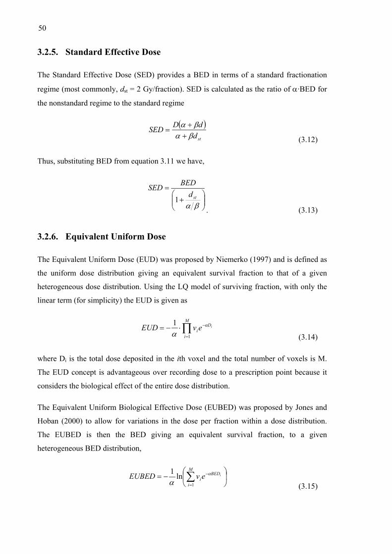
50
3.2.5. Standard Effective Dose
The Standard Effective Dose (SED) provides a BED in terms of a standard fractionation
regime (most commonly, dst = 2 Gy/fraction). SED is calculated as the ratio of α·BED for
the nonstandard regime to the standard regime
( )stddDSED
βαβα
++
= (3.12)
Thus, substituting BED from equation 3.11 we have,
+
=
βαstd
BEDSED1
. (3.13)
3.2.6. Equivalent Uniform Dose
The Equivalent Uniform Dose (EUD) was proposed by Niemerko (1997) and is defined as
the uniform dose distribution giving an equivalent survival fraction to that of a given
heterogeneous dose distribution. Using the LQ model of surviving fraction, with only the
linear term (for simplicity) the EUD is given as
∏
=
−⋅−=M
i
Di
ievEUD1
1 α
α (3.14)
where Di is the total dose deposited in the ith voxel and the total number of voxels is M.
The EUD concept is advantageous over recording dose to a prescription point because it
considers the biological effect of the entire dose distribution.
The Equivalent Uniform Biological Effective Dose (EUBED) was proposed by Jones and
Hoban (2000) to allow for variations in the dose per fraction within a dose distribution.
The EUBED is then the BED giving an equivalent survival fraction, to a given
heterogeneous BED distribution,
−= ∑
=
−M
i
BEDi
ievEUBED1
ln1 α
α (3.15)

51
where BEDi is calculated for voxel, vi, from the total number of fractions with equation
3.8. The EUBED can also be expressed in terms of EUD for the cases of constant number
of fractions or constant fraction size (Jones and Hoban, 2000). This conversion is useful
because most clinicians will relate clinical outcomes to dose, or a certain fractionation
regime.
3.3. Tumour Control Probability
The probability of killing all tumour cells in the defined tumour volume following
irradiation to a certain total dose is named the Tumour Control Probability (TCP). All
clonogens need to be eradicated to achieve tumour control since, theoretically, only one
tumour cell is required to repopulate the tumour.
For calculation, the tumour volume is considered to be contructed of independent tumour
subvolumes (Webb and Nahum, 1993). If each subvolume is considered small enough to
receive a uniform dose then the TCP for the tumour is simply the product of the TCP
values calculated in each of the M subvolumes:
. (3.16) ∏=M
iiTCPTCP
The probability that all clonogens will be killed by total dose, D, in fractions of dose, d, for
the subvolume will be given by the LQ expression for cell killing (from equation 3.6)
[ ].exp )( dDt eVTCP βαρ +−⋅⋅−= (3.17)
Similarly, an expression for TCP using the Biological Effective Dose is;
[ ]BEDt eVTCP ⋅−⋅⋅−= αρexp (3.18)
Following equation 3.17, the expression may be rearranged to calculate the total dose, D,
required for a given value of TCP neglecting the β term;
(
⋅
−−= TCP
VD
t
ln1ln1ρα
) (3.19)
52
Equation 3.19 implies that for a constant TCP the dose required will vary in proportion to
reciprocal cell sensitivity, 1/α, the natural logarithm of clonogen density, ln(ρ), and the
natural logarithm of tumour volume, ln(Vt). Therefore changes in the cell sensitivity or
dose can have a large effect on the TCP. For example, for 0.1 < TCP < 1 the treatment
dose will vary by only about 10 Gy for cell sensitivity of 0.35 Gy-1.
3.3.1. Accounting for interpatient radiosensitivity variation in a
population of patients
Clinical measurements of cell cultures have shown variation in surviving fraction across
the population of tumour types, across samples of the same type of tumour, and within a
single tumour. Clinically, a given type of tumour will then be characterised by a mean and
standard deviation of cell sensitivity from measurements made across a patient population.
The impact of interpatient variations in cell sensitivity will be a decrease in slope of the
population mean tumour control curve from the TCP curve for an individual patient.
Population TCP curves are illustrated in figure 3.4 for α=0.35 Gy-1 with σα=0 or 0.08 Gy-1
(Webb and Nahum 1993).
For an individual patient the TCP curve will be steeper than the population average and
close to the curve in figure 3.4 with σα=0. Intratumour variation (due to a hypoxic fraction,
for example) in cell sensitivity will cause a decrease in the slope of the TCP curve for an
individual patient (Niemerko and Goitein, 1991). For an individual patient, the clinician
will always prescribe a dose level to terminate the least sensitive cells in the tumour.
Importantly, the variation in cell sensitivity for a single patient is hypothesised to be small,
and will be closer to the theoretical TCP versus dose curve without variation, than to the
less steep population TCP versus dose curve (Zagars et al 1989).
3.3.2. Clonogen density and optimisation
A number of studies in the literature have investigated the influence of the spatial
distribution of clonogens, as well as inter- and intratumour radiosensitivity variations on
the dose distribution required to optimally eradicate the tumour.
Obviously, a uniform dose distribution will yield optimum TCP (Brahme and Ågren 1987,
Webb, 1993) if the clonogens are distributed uniformly. However, the spatial distribution

53
of clonogens is probably not uniform, and a number of workers have investigated the
influence of heterogeneous clonogen distributions on TCP. In particular, from equation
3.19, the dose required for constant TCP will decrease with the natural logarithm of
clonogen density. Therefore, large decreases in clonogen density, such as across
microscopic extensions at the tumour periphery, will still require a significant dose for
tumour eradication (Webb and Nahum 1993).
SD=0.00 SD=0.08
Figure 3.4 Characteristic sigmoidal TCP versus dose curve derived theoretically and experimentally. (Taken from Webb and Nahum 1994)
The optimal dose distribution regarding intratumour variation in the cell sensitivity will
show significant variation accordingly. Considering the example from Ebert and Hoban
(1996) for a tumour with cell sensitivity 0.35 Gy-1, an intrinsic spatial variation in cell
sensitivity with standard deviation 0.08 Gy-1 will introduce a difference of about 20 Gy
between the TCP curve with uniform and optimal dose distributions. The optimal TCP
includes increased dose for those voxels with lower than average cell sensitivity and vice
versa. Indeed, a number of authors have investigated how to include intratumour variation
in cell sensitivity so that when more data is available, dose distributions can be optimised
accordingly (Brahme and Ågren, 1987). In the meantime, Kåver et al (1999) have
suggested a method to stochastically optimise TCP based on a known variation in
interpatient cell sensitivity.
54
3.3.3. Prostate Carcinoma
Prostate carcinoma is a slowly proliferating tumour, with estimates of the median potential
doubling time, Tpot = 42 days calculated from a range of 15 to 170 days across the patient
population (Haustermans and Fowler 2001). The half life for sublethal damage repair, T1/2
= 1.9 hrs (95% CI 1.4-2.9 hrs, Fowler et al 2001). The cell sensitivity for prostate
carcinoma, α, has been estimated at 0.29 ± 0.07 Gy-1 (Sanchez-Neito and Nahum, 1999).
The α/β ratio for prostate carcinoma is currently being reevaluated, with some researchers
estimating its value as 1.5 Gy (95% CI 0.8-2.2, Brenner and Hall 1999) and 1.49 (95% CI
1.25 to 1.76, Fowler et al 2001). These reported values are substantially lower than the
traditionally accepted value of 10 Gy for most tumour cells. The reevaluated value of α/β
ratio is now close to (and even lower than) the best estimate value for normal tissue (α/β=3
Gy). The low α/β ratio for prostate cancer might be explained by the low cell cycle rate,
and high proportion of cells in the G0 phase of the cell cycle.
The ramifications of a low α/β ratio is that the tumour will be less sensitive to fractionation
effects. That is, the tumour will respond similarly to normal tissue. The benefit from
fractionation is that with each fraction an incremental separation of the late (normal tissue)
and early (tumour) effects. New fractionation regimes could therefore be an improvement
on the current techniques, and may make much more difference than improvements in the
conformality of dose delivery. One such fractionation regime being discussed in the
literature is hypofractionation. This regime considers reducing the total target dose
appropriately such that the dose per fraction could be increased with no change in tumour
control and late sequelae expected.
Such schemes have been used in some centres in Britain for 20 years. Most well known is
the 6 × 6 Gy regime, which has shown similar survival and complication rates to the more
conventional 1.8 to 2 Gy per fraction regimes. Further indications for hypofractionation are
found in a recent publication that compared two boost doses for prostate, 2 × 9 Gy
compared with 3 × 6 Gy (Martinez et al 2000). In that study, the former regime with the
larger boost fraction size was shown to cause significantly higher survival rates than the
smaller boost fraction size regime.

55
The hypofractionation regimes are (Brenner 2000)
as efficacious as standard fractionation ο
ο
ο
more convenient for the patient, both in terms of logistics and acute morbidity
less resource intensive.
More clinical trials of hypofractionation regimes are currently in progress, and the
conventional fractionation regimes will continue to be favoured until further positive
findings are reported.
Some centres (such as Memorial Sloan Kettering in the United States) are currently
delivering large doses (>80 Gy) to the prostate with over 40 fractions of 2 Gy. These
treatments require patients to be treated once every weekday over 8 or more weeks. If
target doses as high as 80 Gy are to be prescribed a hypofractionation regime will be well
tolerated by the patient due to lowering the total time of treatment. Hypofractionation
would also allow more patients to be treated.
In this thesis, the prostate is modelled without the potential doubling time parameters that
would be necessary for other rapidly growing tumours and with the conventional
fractionation of 2 Gy/fn to the target tissue. The fractionation is considered additionally to
the total dose for all tumour control calculations by using the β term in the LQ model.
3.4. Normal Tissue Complication Probability
Normal tissue complication probability (NTCP) is the probability that a certain percentage
of the patient population will incur unfavourable reactions in the contiguous tissue at a
particular dose. Normal tissues will always receive radiation dose with the treatment of
deep-seated tumours with external beam radiation therapy.
3.4.1. Dose-Volume effects
The calculation of NTCP differs directly from the calculation of TCP due to the intended
endpoints differing. For normal tissues, the relative volume of the organ irradiated to
certain dose levels is used to predict the probability of causing complications. The dose-

56
volume relationship will differ for each organ and will generally be a mix of two extreme
cases, where either a critical dose must be reached or a critical volume must receive a
certain dose before complications (or certain known endpoints) arise.
The normal tissue is constructed of functional sub-units (FSU). The irradiation of a single
FSU to a certain dose level might alter the functionality of the organ and cause
complications. If so, then this organ will be classified under the critical element model or
as having serial architecture. Serial organs have a minimal dose-volume effect because
once any of the critical elements are damaged, the function of the entire organ is impaired.
Alternatively, irradiating a certain proportion of the total organ volume may be required
before the functionality of the organ is impaired and complications arise. This is known as
the critical volume model or parallel architecture. In the case of the parallel architecture,
the FSUs may be more correctly termed Tissue Rescue Units since the organ possesses a
certain functional reserve of the Tissue Rescue Unit’s that assist in the repair of the
functionality following partial volume irradiation. The critical element and critical volume
models are extreme cases and most organs will be a combination of the two.
Clinically, the dose-volume effect has been quantified for many organs. The complication
probability has been plotted against dose for esophagus, lung and rectum in figure 3.1. The
dots indicate clinical data points and the curves represent fitted curves that model the data.
Clearly the lung possesses a strong volume effect, whilst the esophagus and rectum are
shown to be highly serial.
3.4.2. Lyman-Kutcher-Burman (LKB) model
The dose-volume relationship can be represented by the model suggested by Lyman
(1985). The volume effect is described using the parameter n in the power law (Withers et
al 1986, Schultheiss et al 1983)
(3.20) nvvTDTD ⋅= )()1( 5050
where TD(1) is the tolerance dose (i.e. that dose causing a known endpoint to 50% of the
population after 5 years) following whole organ irradiation, and v is the partial volume
defined as v = V/Vref, where V is the total volume of the organ and Vref is the reference
volume, n is a fitting parameter accounting for the volume effect. The reference volume

57
a)
b)
c)
would usually be the whole volume.
Figure 3.5 The dose-volume relationship for a) the (mostly serial) esophagus, b) the (mostly parallel) lung,
and c) the rectum. Taken from Burman et al (1991) using data from Emami et al (1991).

58
The normal tissue complication probability for uniform dose D to a volume V of the organ
is given by
( )dttNTCP
t
.2exp21 2
∫∞−
−=π (3.21)
where
( )( )vTDm
vTDDt
50
50
⋅−
= (3.22)
The mean tolerance dose is defined from TD50(v) and m is another fitting parameter that
accounts for the volume effect. Three parameters are then required {i.e. TD50(1), m, n} to
define the probability of complications for any organ irradiated to uniform dose, D. Table
3.1 includes magnitudes of various parameters used to describe the response of normal
tissues to partial volume irradiation (from Burman et al 1991, Kallman et al 1992).
Table 3.1 Magnitudes of parameters m,n,D50, s and k used to model normal tissue complications following full volume irradiation for a range of organs. From Burman et al (1991) and Kallman et al (1992).
Organ m n D50 (Gy) s k
Brain Stem 0.14 0.16 65 - -
Esophagus 0.11 0.06 68 3.4 0.47
Liver 0.15 0.32 40 0.23 2.6
Lung 0.18 0.87 24.5 0.0061 3.0
Rectum 0.15 0.12 80 - -
Kidney 0.10 0.70 28 - -
Bladder 0.11 0.50 80 1.3 2.9

59
To extend the Lyman model to allow inclusion of heterogeneous dose distributions, the use
of Dose Volume Histograms (DVH) has been proposed by Kutcher and Burman (1989).
Kutcher and Burman (1989) proposed a technique to reduce a histogram featuring various
discrete volumes with certain levels of dose into a single dose bin. Following Lyman, they
conjecture that each dose element of the differential DVH has the same three parameter
values as the whole organ, therefore each dose bin of height ∆Vi and dose Di is adjusted to
one with smaller volume ∆Veff and dose Dm using:
( )
n
m
iiieff D
DVV1
∆=∆
(3.23)
This volume reduction is repeated for each dose element of the DVH until a single bin is
derived with dose Dm and effective volume:
∑ ∆⋅
= i
n
m
ieff VD
DV1
(3.24)
The effective volume, Veff receiving dose Dm can then be used with equations 3.1, 3.3, or
3.6 to compute NTCP.
3.4.3. Källman k- and s-models
A relationship between NTCP predictions from whole, P(D,1), and partial, P(D,v), volume
irradiation was suggested by Källman et al (1992),
( ) ( )[ ] kvDPvDP−
= 1,, (3.25)
where the parameter, k, reflects the magnitude of the volume effect. A large value of k
infers a mostly parallel organ (see table 3.1) and vice versa. At k=-1, equation 3.25 would
be the Poisson model for cell killing, but because P(D,v) must increase as the volume
increases, k>0 (Zaider and Amols, 1999). Kallman et al (1992) originally used vk in
equation 3.25, with k<0.
Introducing the linear part of the LQ model for P(D) in equation 3.25, we have;

60
( )
−= − D
k evNvDP α0exp),(
(3.26)
Källman et al (1992) also describe a technique for considering the architecture of the organ
with a parameter, the relative seriality, s. The relative seriality is derived from the case
where an organ contains relative fractions of serial (0<a<1) and parallel (0<b<1) portions
in its volume. Using the simplifying assumption that b=1, the relative seriality can be
defined from the number of serial, n, and the number of parallel, m, subunits in the
organ, ( ) nmnms 1=⋅= . Low values of relative seriality infer a mostly parallel organ,
while large values infer a mostly serial organ (see table 3.1). For a homogeneous dose
distribution the NTCP is calculated as
( )[ ] ssDPNTCP1
)(11 −−= , (3.27)
where P(D) is the probability for cell killing following dose, D. Using the LQ model, an
expression for P(D) is given in equation 3.7 (above). Extending the model for
inhomogeneous doses, we have
( )
sM
i
vsiDPNTCP
1
1
)(11
−−= ∏
=
∆
. (3.28)
Where the ith voxel receives dose Di, the total number of voxels is M and the relative
volume of each voxel, ∆v = 1/M.
3.4.4. Yaes-Kalend/Fenwick model
For serial organs, the original definition states that local failure (i.e. complications) may
arise following inactivation of an entire FSU consisting of N cells (Niemerko and Goitein,
1991, 1993, Fowler 1993). However, Yaes and Kalend (1988) had previously suggested
that local failure may follow inactivation of any N consecutive cells, out of the N×NF = K
cells, lying along the length of the irradiated volume, where there are NF traditional FSUs.
Following these concepts, Yaes and Kalend derive,
NTCP ~ 1 – exp[-NF(1+Nexp(-α2D))exp(-Nexp(-α2D))] (3.29)

61
where α2 = (1+2β/α), with α and β from the linear quadratic model.
Fenwick (2001a) discovered an error in the derivation of Yaes and Kalend and using a
different method derived,
NTCP ~ 1 – exp[-NFN(1+Nexp(-α2D))(1-exp(-α2 D))N] (3.30)
for the same case, given three conditions. The conditions include NF ≥ 30, 10 < N < 1011,
and (N+1)(1-P)>1, where P is the probability of cell death after a radiation dose, D. When
the conditions are satisfied equation 3.30 leads to an inaccuracy of less than [-2.2%,
+2.5%].
3.4.5. Clinical application of NTCP
A lack of clinical data on normal tissue response due to insufficient dose-volume
availability and recording has lead to NTCP being a less reliable parameter than TCP.
Current treatment planning software does provide facilities for recording complete 3D dose
statistics, that, when aided by patient reviews, is contributing increasing amounts of data. It
is important to note that, as with TCP, the NTCP calculation has limited quantitative
significance but can be beneficial for deciding between competing treatment plans when
assisted by clinical knowledge.
A major shortfall with the current data is a lack of complication information relating to
actual dose distributions. Most of the current models are based on interpolation between
‘known’ complications from whole organ irradiation and partial volume irradiation, where
part of the organ receives a uniform dose and the remainder receives none. This
requirement is evident from the Kutcher-Burman technique for reducing a dose volume
histogram into a partial volume irradiation and interpolating to ‘known’ whole organ
irradiation parameters. Zaider and Amols (1999) investigated the clinical accuracy of two
NTCP models (Probit and Kallman k-model) for non-uniform dose distributions. They
concluded that the extrapolation to (closer to reality) heterogeneous dose distributions
produced a model dependent NTCP result. Clearly, expertise regarding the origin of the
input parameters and model assumptions is important when implementing the NTCP
models clinically.

62
Moisenko et al (2000) compare four NTCP models (Logit, Kallman k-model, Kallman s-
model and probit). They examined the effect of changes to the dose distribution, in terms
of either increased heterogeneity, boosted CTV dose and boosted total dose, on the change
models prediction of NTCP. This was done using two different dose reduction techniques
(preferred Lyman and Kutcher-Burman). The preferred Lyman technique calculates the
effective dose to the full organ volume. The Kutcher-Burman technique (also known as
the effective volume technique) is outlined in §3.4.3 above. Moisenko et al (2000)
concluded that the relative change in the computed NTCP did depend on the model being
used, but the results were consistent for each model.
3.4.6. Rectal complications
3.4.6.1. Grading rectal complications
External beam radiotherapy will always deposit some radiation dose in the adjacent rectal
tissue. When the deposited dose is too high, rectal complications will occur, including
bleeding, severe proctitis, necrosis, stenosis or fistula. The severity of the complication can
be graded using the RTOG grading system (Lawton et al 1991); grade 0 – no complication;
grade 1 – minor symptoms requiring no treatment; grade 2 – symptoms responding to
simple outpatient management, life style (performance status) not affected; grade 3 –
distressing symptoms altering the a patients life style (performance status) and/or requiring
hospitalisation for diagnosis or minor surgical intervention; grade 4 – major surgical
intervention or prolonged hospitalisation; grade 5 – death. Other grading systems have
been suggested, including the SOMA LENT scale (LENT SOMA, 1995) however the
RTOG grading system appears to be the most widely referenced.
From the literature, the predominant complication studied appears to be long term rectal
bleeding. The rectum is constructed mainly of muscle, but sensitive structures, the
telangiectatic vessels, populate the mucus layer of the rectal wall. These telangiectatic
vessels become the site of radiation induced bleeding.
3.4.6.2. Rectum architecture
The early published data on rectal complications (Emami et al 1991) suggested that the
rectum is a highly serial organ (n=0.12, m=0.15). However, more recent studies comparing
3D conformal techniques with traditional beam arrangements (Boersma et al 1998,

63
Hartford et a. 1996) suggest that the rectum does have a pronounced volume effect. This
conclusion is based on a detected benefit from conformal dose distributions that deposit
less dose in the rectal wall. Lu et al.(1995) demonstrated a clear difference between the
grade 0/1 and grade 2/3 complications based the amount of rectal surface area irradiated to
greater than 65 Gy (see figure 3.6a). They concluded that a Lyman volume parameter n
value of 0.2 (compared with the original calculation of 0.12) might be more appropriate for
severe late rectal complications. Fenwick and Nahum (2001b) suggest that the increased
volume effect evident in these studies might be present for a population of patients due to
inter-patient sensitivity differences. The response of an individual, in similarity with
tumour control, should be much steeper than that averaged across the population.
Dale et al (1999) used softer endpoints as a measure of rectal complication than the RTOG
suggestion, citing them as too severe for patient comfort. Based on a patient questionaire,
Dale et al (1999) suggest that for their softer endpoints, the rectum is indeed a serial
structure. This is demonstrated by comparing the correlation co-efficient of the composite
score (from the questionaire) against the volume of rectum irradiated to be higher at lower
volumes (figure 3.6b). Fenwick et al (2001) have conjectured, however, that the limited
variety in dose distributions used by Dale et al (1999) would not provide the data to detect
a volume effect, even if it was present.
a)Figure 3.6 a) The distribution of rectal surfacgrade of prostate cancer. Taken from Lu et alstrongest at low partial volumes (less than 0.5(1999).
b)
e area irradiated across patients can be separated by the . (1995) b) The correlation between NTCP and volume is ) and for full volume delineation. Taken from Dale et al.

64
3.4.6.3. Dose volume characterisation
Dose-volume histograms of the solid rectum (including contents) have been criticised in
the literature (Lu et al 1995b, Ting et al 1997) because the rectum is a hollow organ and
irradiation of the rectum content will not affect the rate of complications. Therefore, other
dose volume techniques have been suggested, including the dose wall histogram (DWH)
and the dose surface histogram (DSH) and more recently the dose surface map (DSM).
The DWH (Ting et al 1997) requires the inside wall of the rectum to be outlined, which is
often difficult, due to poor contrast between rectum contents and wall tissue. The DWH is
defined as the percentage of rectum wall receiving less than a certain dose. Meijer et al
(1999) have suggested that the DWH can be automatically calculated from the outside wall
contour only by assuming that the sectors of the rectal wall have equal areas.
The DSH (Lu et al 1995, Li et al 1997) is the percentage of mid-rectum wall (area) that
received less than a certain dose. The definitions for the DVH, DWH and DSH are
illustrated in figure 3.7 below.
Inner and outer boundaries
organ wall
DWH
DVH
Tracing giving DSH
DSH
Figure 3.7 A transverse section of the rectum showing different methods of organ delineation for
generating histograms. Adapted from Dale and Olsen (1998).
The DSM (Sanchez-Neito et al 2001a, Hoogeman et al 2001) has been suggested as a
valuable technique to maintain the spatial dose-area information of the hollow organ that is
lost with other techniques. The DSM is constructed by ‘unfolding’ the delineated rectum
wall to obtain a 2D map of rectum length superiorly against the angle subtended
perpendicular to the longitudinal axis of the rectum. The dose values are recorded on this
map and illustrate through, for example, a colour map the regions of high and low dose.

65
The DSM should lead to a better understanding of rectal complications. However, they still
need to be improved since they do not account for the changes in rectal wall volume
through the treatment.
Recently, the DSH has been shown to provide correlation between dose and the incidence
of grade 1-3 rectal bleeding (Fenwick et al 2001). Fenwick and colleagues have
characterised the differential DSH of the rectum from external beam therapy of prostate
carcinoma (see figure 3.8 below) with a number of parameters. The parameters tested to
empirically confirm prediction of late rectal bleeding include (Fenwick et al 2001,
Fenwick and Nahum, 2001);
PDmax is the maximum of the high dose peak, ο
ο
ο
ο
PS is the width of the high dose peak,
PDhi is the maximum (%) dose, and
fhi is the fractional highly dosed rectal surface, which is assessed by fitting a Gaussian
to the high dose peak.
Fenwick et al (2001) then compared the 2 year rectal bleeding outcomes from 79 patients
with the summarised dose distribution data of these patients. They discovered that the area-
normalised integral dose, that is, the average dose multiplied by the total surface area
(including 11 cm of rectum length) correlated well (statistically significant) with the
occurance of grade 1-3 rectal bleeding. Other indications, while not as statistically
significant as the area normalised integral dose, were the average dose, the length
normalised high dose area (calculated from, fhi*L), and the length based integral dose to
the highly dosed area (calculated from, PDhi(Dref/100)fhiL).
Further prognostic factors have been outlined by Jackson et al (2001). They list different
prognostic factors for each of two maximum dose protocols. For the 75.6 Gy protocol, the
factors shown indicate a higher probability of rectal bleeding included a smaller
anatomically defined rectal wall volume, the maximum dose to the rectal wall, enclosure of
the rectal wall contour inside the 50% isodose, a history of diabetes mellitus, and patient
age. For the 70.2 Gy protocol, the prognostic factors included the first and third factors
listed above for the higher dose protocol. Interestingly, the 50% isodose is a prognostic
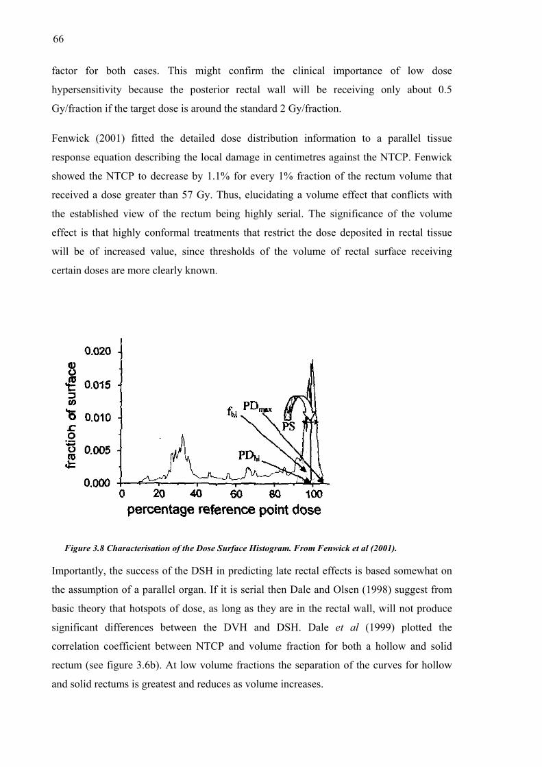
66
factor for both cases. This might confirm the clinical importance of low dose
hypersensitivity because the posterior rectal wall will be receiving only about 0.5
Gy/fraction if the target dose is around the standard 2 Gy/fraction.
Fenwick (2001) fitted the detailed dose distribution information to a parallel tissue
response equation describing the local damage in centimetres against the NTCP. Fenwick
showed the NTCP to decrease by 1.1% for every 1% fraction of the rectum volume that
received a dose greater than 57 Gy. Thus, elucidating a volume effect that conflicts with
the established view of the rectum being highly serial. The significance of the volume
effect is that highly conformal treatments that restrict the dose deposited in rectal tissue
will be of increased value, since thresholds of the volume of rectal surface receiving
certain doses are more clearly known.
Figure 3.8 Characterisation of the Dose Surface Histogram. From Fenwick et al (2001).
Importantly, the success of the DSH in predicting late rectal effects is based somewhat on
the assumption of a parallel organ. If it is serial then Dale and Olsen (1998) suggest from
basic theory that hotspots of dose, as long as they are in the rectal wall, will not produce
significant differences between the DVH and DSH. Dale et al (1999) plotted the
correlation coefficient between NTCP and volume fraction for both a hollow and solid
rectum (see figure 3.6b). At low volume fractions the separation of the curves for hollow
and solid rectums is greatest and reduces as volume increases.

67
3.5. Uncomplicated tumour control and objective functions
The tumour control and normal tissue control probabilities can be used to indicate the
potential for control of the tumour and treatment-induced complications from a given
treatment. However, it is important to be able to combine the positive and detrimental
effects of each treatment into a single parameter, the treatment utility. Naturally, there are
advantages and disadvantages to using a single parameter to decide between competing
treatment plans. Generally the array of biological and dose parameters (including TCP,
NTCP, EUD etc.) should each be considered with clinical expertise.
In its simplest form the treatment utility is given as the uncomplicated tumour control
probability, defined as the probability for controlling a given tumour without
complications;
UTCP = TCP(1-NTCP). (3.31)
The UTCP is defined from the tumour TCP, and the predicted complications of a single
nearby healthy organ or tissue. The UTCP will range between zero and unity with the
higher utility inferring the more beneficial treatment plan and is bound by the assumption
that the complications are independent (Ågren et al 1990). Ågren et al (1990) define the
probability for benefit without complications as,
P+ = PB(1-PI | B) (3.32)
where PI | B is the conditional probability for injury provided that the tumour is controlled.
The parameter, P+, must then rely on whether the injury and tumour control are correlated
or independent. If the tumour control and complication are considered to be independent
events then the conditional probability reduces to PI and equation 3.32 becomes
P+ = PB(1-PI ) (3.33)
which is analogous to equation 3.31 above. Alternatively, if tumour control and
complication are considered to be correlated then the conditional probability will equal
unity and according to the Bayes Law
B
IBI P
PP =| (3.34)

68
which yields
P+ = PB-PI (3.35)
for the uncomplicated tumour control. Clinically, only a subpopulation, ϕ of the total
number of patients will get complications independent of the tumour, and a strongly
correlated group (1-ϕ) will also exist, so that the uncomplicated tumour control may be
expressed as:
P+ = PB – PI + ϕPI(1-PB). (3.36)
A general description for the treatment utility might be given as (Schulthiess and Orton,
1985)
( )∏ −⋅=i
ii NTCPTCPU ω1 (3.37)
where a weight, ωi, is given to each of the i organs that might incur deleterious effects
from the treatment. The clinician would be the professional that is authorised to set the
weights given to the importance of avoiding each particular complication and care should
be taken if any correlation exists between tumour control and complication or between
complications. Generally, only one complication is then considered per organ and only
tissues with NTCP calculated will be included.
The utility of the treatment may be used to compare a number of competing treatment
techniques manually or it can be used as a radiobiological objective function in
computerised optimisation routines. The optimisation routines will calculate the optimal
number of beams, their energies, aperture size etc. One of the more important objective
functions (Mohan et al 1992) includes further constraints to that of the utility (as described
above). Mohan et al (1992) suggest that the weight is itself a sophisticated function of the
NTCP. They constrain the weight by various amounts depending on a clinician derived
'acceptable' NTCP value, Pa, a 'critical' NTCP level, Pc, and a corresponding weight or
score, ca, derived from the acceptable NTCP value. The radiobiological objective function
is then;
∏⋅=i
iCTCPF (3.38)

69
where the component scores, Ci, are calculated using;
( )a
ai PNTCPcC −−= 11 for NTCP ≤ Pa (3.39a)
( )ac
cai PP
NTCPPcC−
−= for Pa < NTCP < Pc (3.39b)
Ci = 0 for NTCP ≥ Pc (3.39c)
The term, Ci, is thus derived from a constraining relationship between a score and NTCP,
where the score at a value of NTCP equal to Pa is ca. Examples of the contraints that were
used with this model to derive the relationship between the score and the NTCP include a
dose-volume constraint for normal tissues, a lower limit on the TCP and upper limits on
the skin dose.
3.6. Summary
A number of radiobiological models have been discussed in this chapter, with further
details given to the cases for the tumour control probability of prostate carcinoma and the
normal tissue complication probability of the rectal wall.
The potential discrepancies in delivered dose, from that planned, can be extrapolated
through these radiobiological models to evaluate possible discrepancies in the TCP, NTCP
and UTCP from that calculated with the static planned dose distribution. Such calculations
are performed in Chapter 6. The variation in each of these parameters is also explored for a
range of feasible parameters.
The linear quadratic model will be used to calculate surviving fraction for tumour and
normal tissue. The LQ model provides a feasible estimate of the surviving fraction and has
been used widely in literature. To calculate NTCP for the rectum, the Kallman s-model
will be used. This model was chosen because the rectum is generally considered to be
serial (with a known volume effect component also), the model suits a voxel based
technique and qualitatively at least, the Kallman s-model has been shown to predict the
correct trends given particular DVH input data compared to others in the literature
(Moisenko et al 2000).

70
With the calculations of TCP, NTCP and UTCP performed in this thesis it is important to
understand the assumptions made for derivation of the radiobiological models themselves,
the current clinical uses of the models and their known limits. The current chapter has
served to provide the basis for these qualifications to be made.
71
Chapter 4
Modelling the dosimetric effect of
treatment uncertainty
4.1. Introduction
In this chapter, the dosimetric effects of the treatment process are modelled using Monte
Carlo and convolution techniques. There are many contributing factors to uncertainty in
delivered dose including geometrical, mechanical and computational factors among others.
Ultimately these individual uncertainties contribute to overall uncertainty in the dose
delivered to the patient (tumour and normal tissues). An understanding of the uncertainty
in deposited dose is important because it impacts directly on the treatment planning and
delivery processes.
This chapter begins by reviewing the impact of the treatment uncertainties on deposited
dose, reviewing modelling techniques from the literature and then the concepts of spatial
and dose probability density functions are introduced. A Monte Carlo technique is used to
model the entire treatment process (planning and delivery) for a patient population
including systematic organ motion uncertainty, random organ motion uncertainty and
random setup uncertainty. A novel convolution kernel is derived that includes systematic
organ motion error. This kernel is used with the convolution technique to predict mean
treatment dose across a patient population. Both Monte Carlo and convolution techniques
have the capacity to account for reductions of systematic organ motion error by using
averaged organ positions from multiple pretreatment CT acquisitions. Weekly and daily

72
multiple CT acquisition regimes can also reduce systematic organ motion error and these
are modelled using the MC code.
Modelling the reduction in systematic organ motion errors due to the use of multiple CT
images to average organ location and accounting for this in the treatment planning
algorithm is the predominant novel investigation in this chapter. Variables such as margin
size, as well as the magnitudes of random and systematic organ motion, random setup error
and penumbra gradients are explored. This investigation of uncertainty in deposited dose
leads to a study of the radiobiological effects of the treatment errors in chapter 6.
4.2. Dose uncertainty
Treatment uncertainties hinder the current technological advances in external beam
radiation therapy, such as 3D conformal techniques and intensity modulated therapy.
It is important to differentiate clearly between the different sources of uncertainty in order
to understand the effect between each of them on the resulting treatment dose distribution.
A list of treatment uncertainties and estimates of one standard deviation in dose would
include (Kron et al 1998);
ο
ο
ο
ο
ο
ο
ο
absolute calibration of the treatment machine (1%),
characterisation of the beams (1.5%),
modelling of radiation transport within the patient (2-5%)
day-to-day positioning of the patient (2%)
the constancy of the patients’ geometry during treatment planning and delivery
uncertainty in the clinical description of tumour volume,
accuracy of the dose prescription.
All of the above mentioned factors need to be considered when prescribing dose to treat
the disease. Other documents (such as ICRU-50, 1993) specify requirements for dose
reporting. ICRU-50 requires that an error of 5% in reporting dose to the isocentre is an
acceptable tolerance level. The last four factors listed above are difficult to label with a

73
standard deviation in dose because they involve further geometrical data and require, more
aptly, dose-volume data. The day to day patient positioning uncertainty will introduce a
spatially varying uncertainty in dose as discussed later.
4.2.1. Modelling dose uncertainty
The current literature provides a very limited number of examples of modelling the dose
uncertainty. One of the studies from the literature models the uncertainty in tumour dose
with the assumption that the magnitude of dose deposited in the patient varies normally
about the prescribed dose (Boyer and Schultheiss, 1988). Standard deviations in dose up to
9 Gy were used to estimate the accumulated effect of most physical sources of uncertainty.
Importantly, Boyer and Schultheiss (1988) presumed a spatially uniform uncertainty in
dose to account for all sources of uncertainty. This presumption obviously oversimplifies
the situation for the particular case of geometrical positioning errors. Beam misalignment
due to these positioning errors has demonstrated larger dose variation near the field edges
than in the field centre (Michalski et al 1993) using portal images. That is, lateral shifts of
the patient relative to the beam will cause large fluctuations in dose in the penumbra and
small fluctuations in dose in the more uniform central dose region. Therefore variations in
the daily patient positioning produce position dependent (spatially non-uniform) dose
uncertainty because the amount of dose variation depends on the position of the point of
measurement. Likewise, organ motion will also cause non-uniform dose uncertainty.
4.2.2. Probability density functions for position and dose
Measurements of organ motion and patient position distributions provide the information
to derive spatial probability distribution functions (PDF) for an organ relative to bony
anatomy (organ motion) and for a patient relative to the treatment machine (setup errors).
The random patient setup PDF can be derived for a population and used, for example, to
predict the variability of patient positioning expected. However, it is useful to derive a
relationship between the spatial PDF and the amount of dose variability (dose PDF) due to
the geometric positioning errors.
Direct derivation of the dose PDF has been described in the literature (Leong 1987) using a
precalculated dose distribution. This dose distribution is static, and positional uncertainty is
modelled as movements of the volume. In figure 4.1 three voxels (at radii labelled r3, r4
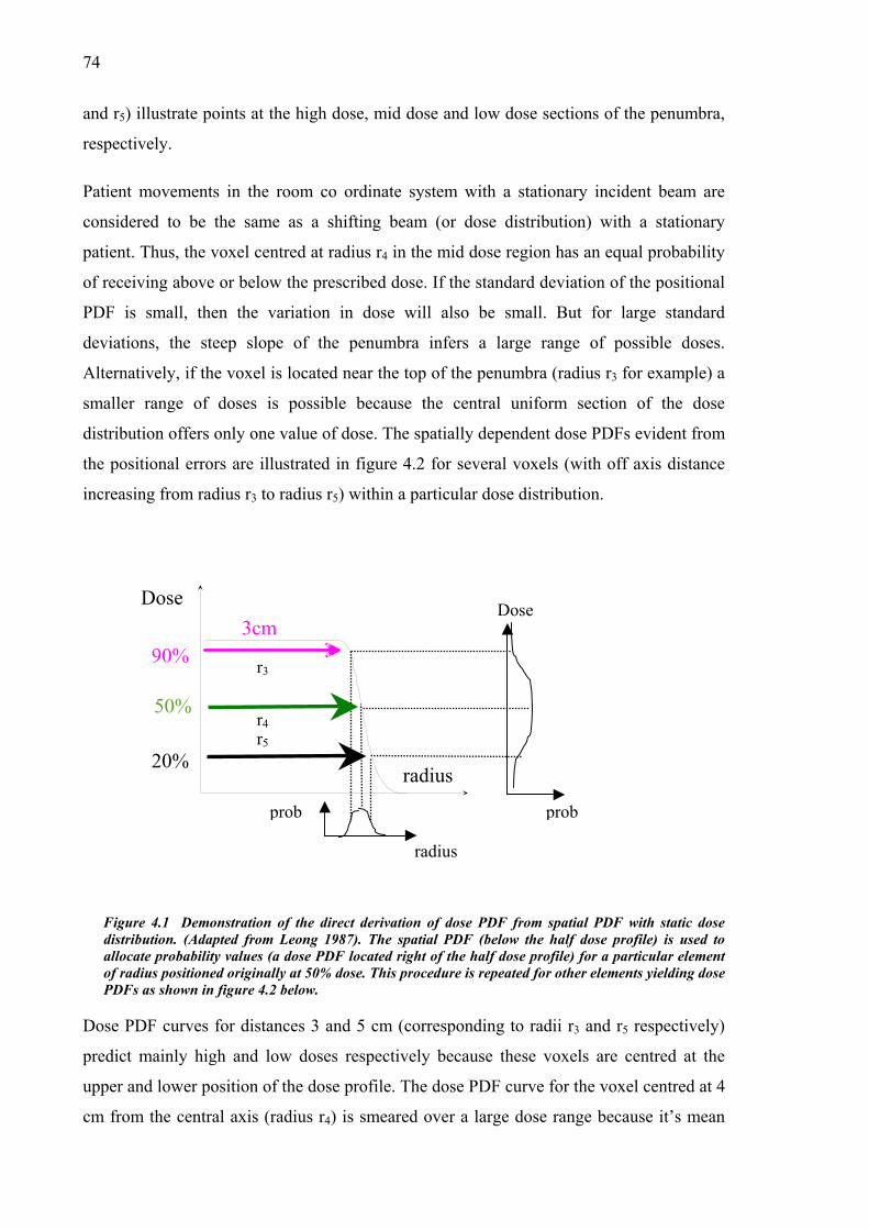
74
and r5) illustrate points at the high dose, mid dose and low dose sections of the penumbra,
respectively.
Patient movements in the room co ordinate system with a stationary incident beam are
considered to be the same as a shifting beam (or dose distribution) with a stationary
patient. Thus, the voxel centred at radius r4 in the mid dose region has an equal probability
of receiving above or below the prescribed dose. If the standard deviation of the positional
PDF is small, then the variation in dose will also be small. But for large standard
deviations, the steep slope of the penumbra infers a large range of possible doses.
Alternatively, if the voxel is located near the top of the penumbra (radius r3 for example) a
smaller range of doses is possible because the central uniform section of the dose
distribution offers only one value of dose. The spatially dependent dose PDFs evident from
the positional errors are illustrated in figure 4.2 for several voxels (with off axis distance
increasing from radius r3 to radius r5) within a particular dose distribution.
Dose
r3
prob
3cm
radius
90%
50%
20%
Figure 4.1 Demonstratiodistribution. (Adapted froallocate probability valuesof radius positioned originPDFs as shown in figure 4
Dose PDF curves for dist
predict mainly high and
upper and lower position
cm from the central axis
prob
n of the direct derivatiom Leong 1987). The sp (a dose PDF located rially at 50% dose. This p.2 below.
ances 3 and 5 cm (c
low doses respectiv
of the dose profile. T
(radius r4) is smeare
radius
r4r5
n of dose PDatial PDF (b
ght of the halrocedure is re
orrespondin
ely because
he dose PD
d over a lar
Dose
F from spatial PDF with static dose elow the half dose profile) is used to f dose profile) for a particular element peated for other elements yielding dose
g to radii r3 and r5 respectively)
these voxels are centred at the
F curve for the voxel centred at 4
ge dose range because it’s mean

75
location is the midpoint of the penumbra. The value of the positional PDF standard
deviation is 0.6 cm.
0
0.05
0.1
0.15
0.2
0.25
0.3
0 20 40 60 80 100Dose (%)
Pro
babi
lity 3.0
3.54.04.55.0
TissueRadius (cm)
r3
r5
r4
Figure 4.2 Dose PDFs within voxels that are positioned at five distances from the cenlabelled from Figure 4.1. Only odd numbered curves are shown for brevity.
4.3. Monte Carlo technique
A Monte Carlo (MC) technique involves modelling physical situations by the
random variables. In this section, the radiotherapy treatment process f
population including treatment planning and delivery is simulated. The M
described here is similar to that described by Killoran et al (1997) that
calculate a statistically oriented planning target volume.
In practice, following cancer diagnosis and the clinician deciding that the
undergo radiotherapy, a number of steps are followed to carry out the radio
first stage is the treatment preparation, which involves the patient having a C
CT image includes a set of transverse 2D images. The tumour volume (GTV)
volume (PTV) are outlined in each of these images and the number and o
incident beams is decided upon. The second step is the treatment delivery.
treatment will be carried out over a number of fractions, with the patient bein
on the couch using lasers in the treatment room against tattoo’s on the patients
D=90%
D=50%
D=20%
tral axis,
sampling of
or a patient
C technique
was used to
patient will
therapy. The
T scan. The
and planning
rientation of
The planned
g positioned
skin.

76
4.3.1. Methods
We first model the imaging and planning process (treatment preparation) and then the
treatment delivery. Interfraction organ motion is typically defined as a translation relative
to bony anatomy, while the setup errors are movements of the bony anatomy relative to the
treatment beam. The modelling uses a fixed grid in the room coordinate system, with axes
in the left-right (x), anterior-posterior (y), and superior-inferior (z) directions.
4.3.1.1. Sampling from distributions, and the dose grid
The Monte Carlo code is written using the Interactive Data Language software1. Random
deviates are calculated by this software using the Box-Muller method (Press 1989).
Organ position at the time of planning CT imaging is sampled randomly from the
corresponding organ motion PDF. This provides organ coordinates, which are then used
through the treatment as a reference for planning and dose delivery. The organ position
used for the treatment planning is determined from at least one CT image. A possibility of
using multiple images is also included in the model. Organ position at CT is represented as
a random variable ξ sampled from the PDF of organ motion, which is assumed to be
documented from in-house measurements.
Mean organ position for the planning,ξ , is computed from NCT simulated organ positions
using:
.1
CT
N
ii
N
CT
∑==
ξξ (4.1)
Once the planning organ position is estimated from the CT scan(s) the dose distribution (or
profile in 1D) is centred at that estimated position. The dose distribution is pre-calculated
using the Pinnacle3 software for a 10 cm × 10 cm field of an incident 6 MV photon beam.
The treatment is modelled for each patient of the patient population. This modelling
incorporates organ misplacement from its mean position at CT and treatment delivery.
1 Research Systems Inc.

77
Treatment delivery uncertainties are simulated as translations of the rigid organ from the
mean planning position (figure 4.3b). The reference frame for scoring the dose to the
tumour is fixed with an origin centred over the actual mean organ position (figure 4.3a).
y′
FiguretreatmsystemThe 1Dpositioset (x′,
Patient s
random
therefore
be comb
y
AMean organ position for
Actual meanorgan position
B
ξ
4.3 (a) Mean organ pent, due to CT uncertainty, th (the x′,y′ co-ordinate system). approach in this study uses o
ns during the treatment delivey′) co-ordinate system.
etup error and organ mo
variables. By using fixed
assume that its variance
ined gaining a treatment d
x
x′ξ
planning
Mean organ position forplanning
x′
y′
φ2
φ1 φ3
osition is represented by the x,y co-ordinate system. In routine e planning image represents the organ in an off-set co-ordinate This co-ordinate system is then used to plan and deliver the dose. nly the x-component of these 2D shifts. (b) Organ ry (such as φ1, φ2 and φ3 for 3 fractions) are measured in the off-
tion uncertainties are both considered as independent
standard deviations for the organ displacement we
does not change during the treatment. These errors may
elivery error
(4.2) .222OMSETD σσσ +=

78
The organ displacement relative to the planned position (incorporating patient setup
uncertainty) at the jth fraction can be represented as a random variable, φj, sampled from
the PDF with variance given in equation 4.2 at each fraction (see figure 4.3b).
Following the jth fraction, the dose distribution will be shifted by a total displacement of
ξφ +=∆ jj (4.3)
from the actual mean organ position.
4.3.1.2. Dose accumulation
For a single incident beam, sample dose, ds(r), is accumulated in voxels following each
fraction. For multi beam treatment, sample dose is combined from all beams and then
accumulated following each fraction. The process is repeated over the course of Nfx
fractions. The value of Nfx in a typical treatment (i.e. ~30) is sufficiently large (Rudat et al
1996) for the discretised distribution resulting from only 30 fractional treatments for each
patient to approximate the continuous distributions used in accordance with the Central
Limit Theorem.
An additional uncertainty in dose due to other factors is also included in the model as a
spatially uniform dose fluctuation in a similar manner to Boyer and Schultheiss (1988).
The relative effect of these components is suggested by ICRU-50 to be less than 5% of the
prescription dose. A uniform component of dose uncertainty is modelled by sampling a
discrepancy from prescription dose, ζ from a normal distribution (with SD=5%, or 0.10 Gy
in the case of 2 Gy fractions) and applied to the existing sample dose fraction.
( ).)()()( ζ⋅+=∗ rdrdrd sss (4.4)
A sample treatment dose for each voxel, Ds(r), is then the sum of the perturbed sample
doses, for the N)(rd s∗
fx fraction treatments:
(4.5) ).()( rdrDfxN
ss ∑ ∗=
For a patient population the values of Ds(r) form a distribution that is used to calculate the
mean and standard deviation of the treatment dose in each voxel.

79
4.3.1.3. Clinical example
Prostate carcinoma has been studied extensively in the literature and was chosen to
investigate the dose uncertainty for a number of reasons. Firstly, interfraction variations in
prostate position have been demonstrated in the literature to approximate a Gaussian
distribution, which is easily implemented in the Monte Carlo (and convolution) codes.
Also, the anatomical position of the prostate implies that patient movements will not affect
the form of the static dose distribution enough to require recalculation for each fraction.
That is, the prostate is distant from significant tissue density changes such as air/tissue
interfaces. The bony pelvis will not affect the dose distribution significantly and therefore
shifts of the beam entry point will not significantly alter the geometry of the combined
dose distributions of the four incident beams.
The dose grid used is sized to include the entire prostate PTV with grid spacing in each
direction of 1 mm. Larger grid spacing was investigated, but is limited by the sensitivity
required with small magnitudes of positional standard deviation.
Table 4.1 Summary of typical error magnitudes concerning supine treatment of prostate carcinoma used for modelling. Delineation error ranges are due to uncertainty in apex and seminal vesicles localisation. Systematic setup errors quoted do not include the use of a correction protocol.
Random error (mm) Systematic error (mm)
Direction LR SI AP LR SI AP
Target delineation
(Rasch et al 1999)
1.7 2-3.5 2.0
Organ motion
(Stroom 1999)
0.6 2.5 2.8 0.5 2.5 2.7
Setup error 3.1 (ref 149) 5.4 (ref 149) 4.9 (ref 149) 2.6 (ref 13) 2.4 (ref 13) 2.4 (ref 13)
Total SD
(quadratic sum)
3.2 6.0 6.1 3.1 4-4.9 4.1
A typical 30 fraction treatment for prostate carcinoma delivering 60 Gy to isocentre was
modelled. We assume that the prostate does not deform or rotate during the treatment.
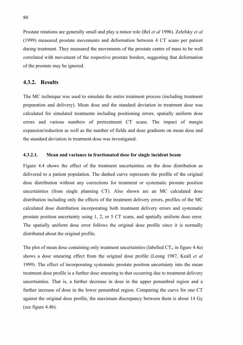
80
Prostate rotations are generally small and play a minor role (Bel et al 1996). Zelefsky et al
(1999) measured prostate movements and deformation between 4 CT scans per patient
during treatment. They measured the movements of the prostate centre of mass to be well
correlated with movement of the respective prostate borders, suggesting that deformation
of the prostate may be ignored.
4.3.2. Results
The MC technique was used to simulate the entire treatment process (including treatment
preparation and delivery). Mean dose and the standard deviation in treatment dose was
calculated for simulated treatments including positioning errors, spatially uniform dose
errors and various numbers of pretreatment CT scans. The impact of margin
expansion/reduction as well as the number of fields and dose gradients on mean dose and
the standard deviation in treatment dose was investigated.
4.3.2.1. Mean and variance in fractionated dose for single incident beam
Figure 4.4 shows the effect of the treatment uncertainties on the dose distribution as
delivered to a patient population. The dashed curve represents the profile of the original
dose distribution without any corrections for treatment or systematic prostate position
uncertainties (from single planning CT). Also shown are an MC calculated dose
distribution including only the effects of the treatment delivery errors, profiles of the MC
calculated dose distribution incorporating both treatment delivery errors and systematic
prostate position uncertainty using 1, 2, or 5 CT scans, and spatially uniform dose error.
The spatially uniform dose error follows the original dose profile since it is normally
distributed about the original profile.
The plot of mean dose containing only treatment uncertainties (labelled CT∞ in figure 4.4a)
shows a dose smearing effect from the original dose profile (Leong 1987, Keall et al
1999). The effect of incorporating systematic prostate position uncertainty into the mean
treatment dose profile is a further dose smearing to that occurring due to treatment delivery
uncertainties. That is, a further decrease in dose in the upper penumbral region and a
further increase of dose in the lower penumbral region. Comparing the curve for one CT
against the original dose profile, the maximum discrepancy between them is about 14 Gy
(see figure 4.4b).

81
-10 -9 -8 -7 -6 -5 -4 -3 -2 -1 0 1 2 3 4 5 6 7 8 9 10
Dos
e (G
y)
0
10
20
30
40
50
60
1 CT 2 CT 5 CT CT∞ Original Dose Profile
The
unc
aro
due
deg
pre
a)
X-Position (cm)
60
~14 Gy
~0.3 Gy
b)X-Position (cm)
4.0 4.2 4.4 4.6 4.8 5.0
Dos
e (G
y)
30
40
50 ~10 Gy
Figure 4.4 (a) Mean dose incorporating uncertainty at both planning and treatment. The dose profile represented by the broken line is the original dose profile and that represented by a solid line includes only the treatment delivery errors. The spatially uniform dose uncertainty follows the original dose profile. (b) Magnified view of penumbra.
maximum discrepancy between the plot with no systematic prostate position
ertainty but incorporating treatment uncertainty (CT∞) and the original dose profile is
und 10 Gy. This illustrates that although most of the differences in mean dose occurs
to the treatment delivery errors, the CT uncertainty does contribute to the dose
radation. After averaging organ position from only two temporally spaced CT images
-treatment, mean dose for the population is within 0.3 Gy of the mean dose calculated

82
with no systematic prostate position uncertainties (indicated by CT∞ in figure 4.4).
Figure 4.5 shows the variation (represented by 1SD) in mean dose to each voxel from the
population of treatments. The plot including treatment delivery uncertainty only is again
represented as CT∞ scans. Figure 4.5 highlights the spatial variation in dose uncertainty
due to positioning uncertainties, with peaks occurring in the penumbral regions of the dose
profile. These peaks are largest at the point of inflection in the dose profile.
Distance X (cm)
-10 -8 -6 -4 -2 0 2 4 6 8 10
Dos
e V
aria
tion,
1SD
(Gy)
0
2
4
6
8
10
12
14 1 CT 2 CT 3 CT 5 CT 10 CT 20 CT CΤ∞
S.U. (5%)
Figure 4.5 Dose variation (1 standard deviation of mean treatment dose) scored in voxels (∆x = 0.1 cm), using multiple CT scans to estimate mean organ position. The solid line shows dose variation due only to treatment delivery uncertainty. Vertical lines represent position of 95% isodose contour and the dash-dot line represents the spatially uniform dose uncertainty.
Figure 4.5 demonstrates a large reduction in dose variation as the number of CT scans used
to average organ position is increased. When using only one CT image to plan the
treatment the standard deviation of the dose has a maximum value of ~14 Gy, but the
maximum value drops to 11 Gy with 2 CT scans and continues to reduce with further
scans. With infinite CT scans performed the maximum value of the standard deviation in
mean treatment dose calculated is ~4 Gy. Over 20 CT scans are needed to reduce the
standard deviation to below the 5 Gy level. More importantly, the dose standard deviation

83
within 95% isodose line (which is often used to treat planning target volume is ~10 Gy for
one CT scan, dropping to 3 Gy with the number CT scans exceeding 10.
Incorporating the spatially uniform component of dose uncertainty results in dose variation
that is proportional to the original dose profile (by definition). The uncertainty of 5% per
fraction (σd= 0.10 Gy) is reduced for the 30 fraction treatment by √30 (refer to figure 4.5).
Thus in the central region of the dose profile where the dose is homogeneous and
prescribed at 60 Gy, the standard deviation in mean treatment dose due to a 5% fractional
dose uncertainty is σD = 0.55 Gy.
4.3.2.2. Impact of margin size
The size of the CTV→PTV margin will obviously affect the position of the 95% isodose
and the entire dose distribution. For shrinking CTV→PTV margins, the penumbra
becomes closer to the tumour periphery as the margin is decreased (refer to figure 4.6a).
Thus the uncertainty in dose will also move closer to the tumour periphery. However,
averaging multiple organ locations from corresponding images will reduce the systematic
organ motion error and this can be used to justify potential margin reductions (as to be
discussed in §4.3.3.1).
Obviously reducing any component of the total treatment error will allow margin
reductions, and this will lower the dose deposited in contiguous normal tissue. Multiple
pretreatment CT scans reduce the uncertainty in mean dose.
4.3.2.3. Impact of magnitude of patient positioning and organ variations
Figure 4.7 shows the variation in treatment dose considering a range of targeting
accuracies. As the standard deviation of positioning error increases, the slope of the dose
distribution decreases. This has been demonstrated experimentally using radiographic film
(McCarter and Beckham, 2000). For each institution it is important to measure individual
values of patient setup and organ position variability.
4.3.2.4. Number of fields and dose gradients.
The number of fields and beam shaping technique used will influence the dose gradient of
the penumbra. The number of fields has been included into margin ‘recipes’ (refer to §2.7).
As the penumbra becomes steeper, that maximum of dose uncertainty increases. This is

84
particularly important for intensity modulated and highly conformal dose delivery
techniques.
60
70
PTV15PTV10PTV5CTV
a)Position - X (cm)
0.0 0.5 1.0 1.5 2.0 2.5 3.0 3.5 4.0 4.5 5.0 5.5 6.0 6.5 7.0
Dos
e (G
y)
20
30
40
50
1.5 cm 1.0 cm 0.5 cm
Margin Size
men
t dos
e (G
y)
5
6
71.5cm 1.0cm0.5cm
b)Off-axis distance (cm)
0 1 2 3 4 5 6 7Sta
ndar
d de
viat
ion
in tr
eat
0
1
2
3
4CTV
Figure 4.6 a) One dimensional profiles of prescribed dose distributions with three margin sizes (0.5, 1.0, 1.5 cm) and b) the associated standard deviations in treatment dose.

85
4.3.3. Discussion
4.3.3.1. Possible margin reductions with multiple pretreatment CT scans
As shown previously, multiple pretreatment CT scans can be used to significantly reduce
the standard deviation in treatment dose, particularly in the penumbra. Conversely, when
the margins are reduced for this standard treatment, the penumbra (and peak of the
standard deviation in treatment dose) will approach the CTV. These two effects may be
combined to justify margin reductions. Figure 4.8 demonstrates that if the standard
treatment utilises one planning CT scan and a margin of 1.5 cm, then an equivalent amount
of dose uncertainty at the tumour periphery is present with either 4 pretreatment images
and a 1.0 cm margin or 30 pretreatment images and a 0.5 cm margin. The mean dose at this
point on the tumour periphery will not differ from that prescribed if the positioning errors
are in the average range.
02468
1012141618
0 2 4 6
Radius (cm)
0.6cm0.8cm1cm
Tumour Position (1SD)
PTV
CTV
Figure 4.7 Standard deviation in treatment dose using the standard deviation in position to be 0.6, 0.8 and 1.0 cm. The value given as ‘tumour position’ is the standard deviation equal to the quadratic sum or random interfraction organ motion and random setup errors.
4.3.3.2. Relative importance of systematic and random components
Intuitively it would seem that systematic prostate position uncertainty, being a systematic
error for each patient, would have a greater detrimental effect on the treatment outcome
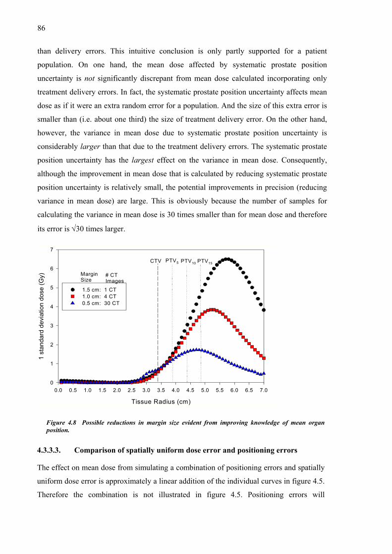
86
than delivery errors. This intuitive conclusion is only partly supported for a patient
population. On one hand, the mean dose affected by systematic prostate position
uncertainty is not significantly discrepant from mean dose calculated incorporating only
treatment delivery errors. In fact, the systematic prostate position uncertainty affects mean
dose as if it were an extra random error for a population. And the size of this extra error is
smaller than (i.e. about one third) the size of treatment delivery error. On the other hand,
however, the variance in mean dose due to systematic prostate position uncertainty is
considerably larger than that due to the treatment delivery errors. The systematic prostate
position uncertainty has the largest effect on the variance in mean dose. Consequently,
although the improvement in mean dose that is calculated by reducing systematic prostate
position uncertainty is relatively small, the potential improvements in precision (reducing
variance in mean dose) are large. This is obviously because the number of samples for
calculating the variance in mean dose is 30 times smaller than for mean dose and therefore
its error is √30 times larger.
Tissue Radius (cm)
0.0 0.5 1.0 1.5 2.0 2.5 3.0 3.5 4.0 4.5 5.0 5.5 6.0 6.5 7.0
1 st
anda
rd d
evia
tion
dose
(Gy)
0
1
2
3
4
5
6
7
1.5 cm: 1 CT 1.0 cm: 4 CT 0.5 cm: 30 CT
CTV PTV5 PTV10 PTV15
MarginSize
# CTImages
Figure 4.8 Possible reductions in margin size evident from improving knowledge of mean organ position.
4.3.3.3. Comparison of spatially uniform dose error and positioning errors
The effect on mean dose from simulating a combination of positioning errors and spatially
uniform dose error is approximately a linear addition of the individual curves in figure 4.5.
Therefore the combination is not illustrated in figure 4.5. Positioning errors will

87
predominately affect the dose delivered to regions of dose gradient at the field edges and
they will be particularly important if sensitive normal tissue abuts the target. The spatially
uniform dose error, which occurs due to such factors as limited linear accelerator
calibration precision, will predominately affect the regions of maximum dose, normally
with in the CTV.
4.3.3.4. Dose reporting
Obviously reductions in mean treatment dose will cause decreases in tumour control
probability (TCP). Importantly, the fluctuations in dose per fraction inferred from the
presented treatment dose variations (refer to figure 4.7) will also have an effect on the
TCP. Increased dose heterogeneity leads to rapid loss in tumour control (Ebert 2000) and
therefore the TCP reduction due to temporal fluctuations will be present in addition to the
loss of tumour control due to mean dose reductions (smearing) caused by the uncertainties
for the population. This indicates that treatment outcome is dependent on both mean dose
and its variance, and that both of these quantities should be indicated on the treatment
plans. Some biological parameters are calculated with the Monte Carlo model developed in
this section in Chapter 6.
4.4. Convolution technique
A convolution method has been used to predict mean dose incorporating the treatment
delivery errors (Leong 1987, Bel et al 1996, Lujan et al 1997, Keall et al 1999). It was
extended to calculate dose variance (Zavgorodni 1997, 2000, Lujan et al 1999). The
convolution equation used to predict the mean dose is of the form:
( ) ( ) zdydxdzyxfzzyyxxDD ′′′⋅′−′−′−= ∫∫∫ ,,,,0 (4.6)
where D0 is the static reference dose and ( )zyxf ,, is a variation kernel, which is usually
assumed to be Gaussian, hence:
( ) ( )( ) ( ) ( )
−+
−+
−= 2
2
2
2
2
2
3 222exp
2
1,,z
z
y
y
x
x
zyx
zyxzyxfσµ
σµ
σµ
πσσσ (4.7)
where µx is the mean x value, which is zero, and σx is the standard deviation in the x

88
direction as prescribed by equation 4.2, and so on.
4.4.1. Derivation of spatial PDF including systematic organ motion
error
The variation kernel used with the convolution method can be extended using statistics to
include systematic organ motion error from the planning stage. The organ mobility affects
delivered dose twice: initially through planning on a potentially displaced image and later
during the treatment delivery (van Herk et al 1995). For a particular patient the CT
uncertainty will result in a systematic positioning error that can be considered random over
a patient population. The individual shifts at each treatment fraction form the treatment
delivery uncertainty distribution. This distribution combines the effects of the organ
motion at treatment with set-up errors and it is fixed for the population of treatments. As a
result, the total variance of positional error distribution for a population of patients is
the sum of the three components
2Tσ
(4.8) 2222OMSEOMT Σ++= σσσ
where and OMΣ OMσ are both related to organ motion, but different notation is used to
separate the systematic from the random component, respectively.
Equation 4.8 is true for the case of a single CT image used to plan the treatment, but
clearly the definition of organ position at planning will become more accurate as further
CT scans are performed. After NCT images are averaged, the standard error in the mean
( ) should be used in this equation to specify the CT component of the total variance.
This component is reduced from its original value by a factor of N
2,CTsσ
CT as follows
CT
CTCTs N
22,
σσ = . (4.9)
Consequently, with multiple pretreatment CT scans used to estimate mean organ position,
the variance of the convolution variation kernel will become
CT
CTOMSET N
2222 σ
σσσ ++= . (4.10)

89
The convolution method was implemented using equations 4.6, 4.7, and 4.10 to compute
mean treatment dose with various NCT and the results compared to the benchmark MC
results. The use of convolution technique allows the integration of this approach into the
treatment planning software.
4.4.2. Benchmarking against Monte Carlo results
Figure 4.9 demonstrates that systematic prostate position uncertainty can be easily
accounted for in the treatment planning calculations. Shown in this figure is the mean dose
for a patient population calculated using the convolution method with the variation kernel
that includes the effect of systematic prostate position uncertainty through equation 4.10.
An excellent agreement is observable between the convolution and the MC results
(replotted from figure 4.4). Treatment planning software corrections used to account for
the treatment uncertainties are further investigated in Chapter 7.
4.4.3. Margin recipe including systematic error
The systematic organ position error is reduced when the average organ position is used
from multiple pre-treatment image acquisitions. The CTV→PTV margin ‘recipes’ (refer to
§2.7) include a factor of 2.5 times the standard deviation of systematic error. This standard
deviation is the quadratic addition of systematic patient setup (ΣSE) , systematic organ
localisation (ΣOM) and delineation error (Σdelin). Multiple pretreatment imaging can
therefore be directly incorporated into the margin recipe to compensate for the reductions
in systematic organ motion error. The margin for systematic error including the number of
pretreatment images used to derive the mean organ position NCT may be extended from
equation 2.6 using equation 4.9 as;
Hsys = ∑∑ 22
25.delin
CT
OMSE N∑ ++2 (4.11)
For images (megavoltage images or CT) acquired during the treatment the inclusion of
localisation improvements into say shrinking margin recipes would be useful. However,
this would not be as simple to calculate as for the pretreatment image acquisition.

90
Position - X (cm)
0 1 2 3 4 5 6 7
Mea
n Tr
eatm
ent D
ose
(Gy)
0
10
20
30
40
50
60
MC: 1CT CONV: 1CT MC: 5CT CONV: 5CT Original Dose Profile
Figure 4.9 Mean treatment dose predicted for 1 and 5 CT scans using the convolution method as compared with MC results. The original dose profile is also shown.
4.5. Multiple CT scans
The systematic discrepancy between the organ position located during the planning CT
scan and the mean organ position during treatment has been quantified in this thesis (refer
§4.3.2.1) and in the literature (van Herk et al 1995, McKenzie et al 2000). One method to
overcome this is to adapt the delivery following imaging procedures as the treatment
course proceeds. Suggested imaging procedures have included kilovoltage x rays, CT
scans, and ultrasound (Padhani et al 1999, Dawson et al 1998, Lattanzi et al 1999). This
would be similar to patient repositioning following portal imaging to reduce systematic
setup errors. As with the repositioning protocols (refer to §2.6) a variety of regimes are
possible.
4.5.1. Timing regimes for multiple intra-treatment image acquisition
The effect of the frequency of imaging procedures during treatment delivery on the mean
dose and variance in mean dose is investigated in this section. The MC code accounting for
multiple pretreatment imaging (§4.3) is altered here to account for various intratreatment
regimes. In particular; imaging done daily with on-line isocentre shifts, imaging done daily

91
with off-line isocentre shifts using the adaptively improving estimation of mean organ
position, and imaging done weekly with adaptively improving estimation of mean organ
position.
The pseudo code for modelling each of these regimes is included in figure 4.10 a→c,
respectively. In the figures, the MC simulation begins following the initial treatment
preparation with the simulation of Nfx treatment fractions. Any given treatment fraction
may be given following the NCT CT image acquisition sessions.
a) b) c)
Yes
No
Calculate total shift and add dose to dose grid
Use improved organ position
NCT/5 ∈ 9?
Simulate fraction
Yes
No
Calculate total shift and add dose to dose grid
Use improved organ position
Is N<NCT?
Simulate fraction
Yes
No
Calculate total shift and add dose to dose grid
Use exact daily organ position
Is N<NCT?
Simulate fraction
Figure 4.10 Flow chart of regimes for timing multiple imaging
Regime ‘a’ specifies CT image acquisition daily with on-line shifting of the patient
through the initial portion of the patients’ treatment. This regime assumes that the patient
does not move between the daily imaging procedure and treatment fraction. For this an
immobilisation device would be used. The literature provides one example of regime ‘a’ in
practice, which studied the resulting patient positioning uncertainty (Lattanzi et al. 1998).
In practice, regime ‘a’ would be time consuming and restrictive for the patient.
Regime ‘b’ includes daily imaging of the patient with off-line shifting of the patient.
However, the patient is allowed to walk from the imaging venue to the treatment couch,
and the daily organ position is used to improve the average organ position. Although more
practical and comfortable for the patient, if significant improvements in dose deposition
accuracy are not present then the workload involved with utilising all the extra information
would probably be limiting. Of course, some studies of prostate motion indicate that inter-
fraction variations decrease as the treatment progresses and this suggests that only the first
portion of the treatment might feasibly be imaged.

92
Regime ‘c’ specifies imaging only once per week. This is expressed mathematically in
Figure 4.10 as when the total number intended divided by the number of days in the week
is an integer. Regime ‘c’ implies a similar imaging workload to regime ‘b’ with Nfx=5.
However, with regime ‘b’ the improved organ location estimate is used for the remaining
weeks of treatment, while the same precision is acheived with only days remaining for
regime ‘c’.
4.5.2. Results
Incorporating regimes ‘a’, ‘b’, or ‘c’ into the treatment process modelled with the MC code
is illustrated for mean dose and spatial variance in mean dose.
The curves for both mean dose and one standard deviation in dose (refer to figure 4.11) for
the on-line technique (regime ‘a’) are demonstrated to be similar to the daily CT offline
technique (regime ‘b’). If daily CT scans were to be used, then the daily offline over the
first week of treatment will provide the most advantage considering usefulness and staff
workload. Clinically, all of the multiple imaging techniques would obviously be combined
with portal imaging schedules for correcting systematic patient setup error (refer to §2.6).
4.6. Monte Carlo modelling of 3D dosimetric impact
The Monte Carlo method (outlined in §4.3) was used to calculate mean treatment dose and
the standard deviation in mean treatment dose, incorporating clinically feasible
uncertainties in the delivery of the four field ‘box’ technique (with rectangular fields)
commonly employed to treat patients with prostate carcinoma. The prescribed treatment
included 64 Gy to be deposited at isocentre in 32 fractions.
4.6.1. Methods
The dose distribution from the four field treatment of a patient treated for prostate
carcinoma was extracted retrospectively from the treatment planning system2. The dose
distributions for each of the four beams were separately calculated forming a set for that
2 Pinnacle v5.2g

93
PTV margin. Three uniform PTV margins were used (0.5, 1.0, 1.5 cm) each composed of a
set of four dose distributions. The dose grid encompassed the largest PTV and the rectum
with an additional margin around both. Dose calculation used the Pinnacle
convolution/superposition algorithm with 0.5 cm voxels. The CTV and three PTVs are
illustrated in figure 4.12 with the structures of interest (i.e. prostate and rectum).
ion
in m
ean
dose
(Gy)
3
4
5
6
7
1 CT day 2 CT days 3 CT days 5 CT days 10 CT days 20 CT days
Dos
e (G
y)
50
55
60
65
1 CT day 2 CT days
a)Off-axis distance (cm)
0 1 2 3 4 5 6
Stan
dard
dev
iat
0
1
2
Off-axis distance (cm)
0 1 2 3 4 5 6
Mea
n
35
40
453 CT days 5 CT days 10 CT days 20 CT days Original Dose
se (G
y) 55
60
65
1 CT day n in
mea
n do
se (G
y)
4
5
6
71 CT day 2 CT days 3 CT days 5 CT days 10 CT days 20 CT days
b)Off-axis distance (cm)0 1 2 3 4 5 6
Mea
n do
35
40
45
502 CT days3 CT days 5 CT days 10 CT days 20 CT days Original Dose
Off-axis distance (cm)
0 1 2 3 4 5 6
Stan
dard
dev
iatio
0
1
2
3
n D
ose
(Gy)
50
55
60
65
1 CT week 2 CT weeks in
mea
n do
se (G
y)
3
4
5
6
1 CT week 2 CT weeks 3 CT weeks 4 CT weeks 5 CT weeks
c)Off-axis distance (cm)
0 1 2 3 4 5 6
Mea
35
40
45 3 CT weeks 4 CT weeks 5 CT weeks Original Dose Profile
Figure 4.11 Mean dose (a→c) and variancea,b, c into Monte Carlo modelling of the trea
f)
e)
d)
Off-axis distance (cm)
0 1 2 3 4 5 6
Stan
dard
dev
iatio
n
0
1
2
in mean dose (d→f) resulting from incorporating regimes tment process.

94
30
AP
(mm
)
T
d
s
b
s
a) 6030
20
10
10 20 30 40 50
201030
30
30
30
20
20
20
10
10
10
40
404040
40
40 40
50
505050
50
50 50
60
6060
60
60 60
30
30
30
30
20
20
20
2010
10
10
X DataLateral (mm)
0
40
50
Lateral (m10 20 30
AP
(mm
)
0
10
20
30
40
50
60
4040
40
40 40
5050
50
5050
660
60
60 60
30
30
30
20
20
20
10
10
10
Figure 4.12 Illustration of the prostate gland (Gby margins of a) 0.5 cm b) 1.0 cm and c) 1.5 cmgreen volume is the prostate (GTV & CTV) and
he previously described MC technique was
istributions comprising the four field beam
ame sampled shifts of the organ and patien
eam. Following the 32 simulated prescrib
ummed, giving a simulated treatment dose
b)
Lateral (mm)10 20 30 40 50
AP
(mm
)
0
10
20
30
40
50
60 102030
30
30
30
20
20
10
10
40
404040
40
4040 40
50
505050
50
50 5050
60
606060
6060 60
30
30
30
30
20
20
20
10
10
10
102030
40
4050
6060
c)
m)40 50
30
30
20
20
10
10
40
40
50
50
60
0
TV), rectum and three dose distributions characterised . In each case the 95% isodose indicates the PTV, the
the brown volume is the rectal wall.
applied separately to each of the four 3D dose
design for each patient. At each fraction, the
t were applied to the dose distribution of each
ed fractions, the four dose distributions were
distribution. One thousand simulated treatment

95
dose distributions were created and used to calculate the mean treatment dose distribution
and the standard deviation in mean treatment dose.
The convolution technique described in §4.4 was also used to generate mean treatment
dose distributions.
4.6.2. Results
Mean treatment dose distributions calculated with the MC and convolution techniques
coincided. Only the mean treatment dose distributions calculated with the MC technique
are shown.
Mean treatment dose is illustrated in figures 4.13 with 0.5, 1 and 1.5 cm isotropic margins
around the tumour volume. Each contour plot show small variation between the mean dose
distribution considering a single CT used for planning and the original (planned) dose
distribution. The 60 Gy isodose contour of the former is inside that of the latter and vice
versa for the 40 Gy isodose contour, illustrating a reduction of the penumbra gradient with
positioning uncertainty. As with the 1D case, the deviation between the mean dose
distribution based on a single CT scan and that based on an infinite number of CT scans is
very small. The difference between all three cases depends on the penumbra gradient as
evidenced by comparing the discrepancy along the oblique cross section through the
central ‘box’ and the cross section parallel to the axes. A larger discrepancy is present in
the former case due to the higher penumbra gradient.
The mean treatment dose, calculated with only spatially uniform interfraction variation in
dose, follows the original dose distribution.
The standard deviation in mean treatment dose is illustrated in figure 4.14 below in the
transverse slice for the dose distributions including 0.5 and 1.5 cm margins.
For the 0.5 cm margin and in the transverse plane (figure 4.14a) the penumbra is located
between lateral positions {7,12} and {23,27} and anterior-posterior positions {10,15} and
{22,26}. The standard deviation in mean treatment dose, shown as profiles in figure 4.16a,
peaks in these penumbral zones.

96
0 5 10 15 20 25 30
5
10
15
20
25
30
10
10
20
20
30
30
30
20
10
40
40
40
4040
40
10
20
50
50
50
50
50
50
2030
60
60
6060
60
50
30
3030
30
40
20
20
20
20
10
10
10
10
3030
10
10
20
20
30
30
30
30
20
20
10
10
40 40
40
4040
40
40
50
50
50
50
50
50
60
60
6060
60
30
20
20
30
30
20
20
3030
10
10
10
10
10
10
20
20
30
30
30
2010
40 40
40
40
10
20
50
50
50
50
50
50
20
30
30
4040
40
60
60
60
60
60
30
30
30
40
20
20
20
20
10
10
10
10
30 30
Anterior-posterior (Y) cm
Late
ral (
X) c
m
Superior-inferior (Z) cm
0 5 10 15 20
Ant
erio
r-po
ster
ior (
Y) c
m
5
10
15
20
25
30
10
10
10
10
20
20
20
20
30
30
30
30
40 40
40
40
4040
40
50 50
50
5050
50
60 60
60
60
60
30
30
30
50
3020
20
20
20
30
10
10
20
10
10
10
10
10
10
20
20
20
20
30
30
30
30
4040
40
40
4040
40
50 50
50
5050
50
60 60
60
60
60
30
30
30
50
30
30
20
20
20
40
20
10
10
20
10
10
10
10
10
10
20
20
20
20
30
30
30
30
40 40
40
40
4040
40
5050
50
50
5050
50
60
60
60
6060
60
30
30
30
50
30
30
20
20
20
40
20
20
10
10
10
10
0 5 10 15 20 25 30
5
10
15
20
25
30
1020
30
30
30
30
2010
40 40
40
40
4040
40
40
50
50
50
5050
50
50
60
60
60
60
60
60
50
30
30
30
20
20
4020
20
3030
10
10
10
10
1020
30
30
3020
10
40 40
40
40
4040
40
40
50
50
50
5050
50
50
60 60
60
6060
60
30
30
30
50
20
20
4020
20
10
10
3030
10
10
1020
30
30
302010
40 40
40
40
4040
40
40
50 50
50
50
5050
50
50
60 60
60
6060
60
60
30
30
30
4020
20
20
20
3030
10
10
10
10
Anterior-Posterior (Y) cm
Late
ral (
X) c
m
Superior-Inferior (Z) cm
0 5 10 15 20 25
Ant
erio
r-P
oste
rior (
Y) c
m
5
10
15
20
25
30 10
10
10
20
20
1020
20
30
30
30
4040
40
40
50 50
50
50
5050
50
30
40
40
40
40
6060
60
6060
60
50
30
30
30
30
40
20
20
20
2010
10
10
10
10
10
20
20
1020
20
30
30
30
4040
40
40
50 50
50
50
5050
50
30
40
40
40
40
60
60
60
60
60
60
30
30
30
50
30
40
20
20
20
20
10
10
10
10
10
10
10
20
20
20
2030
30
30
30
50 50
50
50
5050
50
40
4040
40
40
4040
40
60 60
60
6060
60
50
30
30
30
30
20
20
20
2010
10
10
Anterior-posterior (Y) cm
0 5 10 15 20 25 30
Late
ral (
X) c
m
5
10
15
20
25
30
35
10
20
20
30
30
30
30
20
10
40 40
40
40
4040
40
40
10
20
50
50
50
5050
50
50
60
60
60
6060
60
30
30
30
40
20
20
20
20
10
10
10
30
10
20
20
30
30
30
30
2010
40 40
40
40
4040
40
1020
50 50
50
50
5050
50
5060 60
60
6060
60
60
30
30
30
40
40
20
20
20
20
10
10
10
10
30
10
20
20
30
30
30
30
20
2010
40 40
40
40
4040
40
40
50 50
50
50
5050
50
50
60 60
60
6060
60
60
30
30
30
20
20
20
20
30
10
10
10
10
Superior-Inferior (Z) cm
0 5 10 15 20 25
Ante
rior-
post
erio
r (Y)
cm
5
10
15
20
25
30
10
10
10
10
20
20
20
20
30
30
30
30
40
4040
40
40
4040
40
50 50
50
50
5050
50
60 60
60
6060
60
50
30
30
30
3040
20
20
20
20
2010
10
10
10
10
10
20
20
20
20
30
30
30
40 40
40
40
50 50
50
50
5050
50
30
40
4040
40
60
60
60
60
6060
60
50
30
30
30
3040
20
20
20
20
10
10
10
10
10
10
10
20
20
20
20
30
30
30
30
4040
40
40
40
4040
40
5050
50
50
50
50
50
50
60
6060
60
6060
60
50
30
30
30
3040
20
20
20
2010
10
10
10
Figure 4.13 Two views of the mean treatment dose calculated with three original dose distributions (for margins of 0.5, 1.0, 1.5 cm) for three cases. The three cases are an original dose distribution (black solid line), a mean treatment dose calculated based on 1 planning CT scan (blue solid) and a mean treatment dose based on infinite planning CT scans (red solid line).
The standard deviation in mean treatment dose is illustrated in figure 4.15 for the scenario
of multiple CT scans (1,2,5, ∝) at planning and uniform dose uncertainty (2% and 5%).

97
The results are shown for each of the three margin sizes along the planes sharing the point
(15,20,12). The standard deviation in mean treatment dose, calculated with only spatially
uniform inter-fraction variation, is proportional to the original dose distribution.
Anterior-posterior (Y) cm
0 5 10 15 20 25 30
Late
ral (
X) c
m
5
10
15
20
25
30 132
55
5 54
4
4 46
66
6 65 5
5 54321
1
1
3
3
2
2
554
44 4
6665
55 54
4
4 432
1
3
7
44
7
66
6
3
3
3
3
3
33
3
3 3
22
2
2
22
21
1
1
1
2 21 1
11
5 56 6
3
7
4 4
7
6 6
3
3
33
33
3
3
6
2
21
1
22
22
2
21
1
1
1
1
Anterior-posterior (X) cm
0 5 10 15 20 25 30
Late
ral (
X) c
m
5
10
15
20
25
30
35
12
4 4 4 43
5 5 5 56
6 6 6 65 5 5 5432
1
12
2
4 4 4 43
3
65 5 5 56
6 6 65 5 5 54 4 4 43 21
344
7
7
66
3
3
3
3 3
3
33
3
3
3 3
66
22
2
2
2
2
2
2
1 1
1
1
1
1
2 2
11
1 1
34
7
7
6
6
3
3
2
3
3
3
3
32
1
2
2
2
1
1
1
1
Figure 4.14 Iso-standard deviation plots in the transverse plane with a) 0.5 cm and b) 1.5 cm margin.
4.6.3. Discussion
The mean treatment dose distributions across a population of patients featuring feasible
magnitudes of error during treatment preparation and delivery have been modelled. Three
original dose distributions were considered to cover the CTV plus margins of 0.5, 1.0, and
1.5 cm.
The discrepancy between planned and calculated mean (actual) dose distributions is shown
to be largest at the junctions of orthogonal beams for the four field box technique.
Accordingly, the standard deviation in mean treatment dose is largest at these four
junctions and peaks with dose ~6.5 Gy.
The spatially uniform dose uncertainty results in inter-treatment variations of treatment
dose with standard deviation, σD ~ 0.6 Gy for the 5% fractional dose error. This variation
between patients prescription doses will occur in the tumour volume.

98 de
viat
ion
in M
TD, G
y
3
4
5
6
71 CT2 CT5 CTCTinfUniform (2%)Uniform (5%)
evia
tion
in d
ose
(Gy)
3
4
5
6
7
a)Lateral (X) cm0 10 20 30
Sta
ndar
d
0
1
2
Anterior-Posterior (Y) cm0 10 20 30
Sta
ndar
d d
0
1
2
dev
iatio
n in
MTD
Gy
3
4
5
6
7
dev
iatio
n in
MTD
, Gy
2
3
4
b)Lateral (X) cm
0 5 10 15 20 25 30
Sta
ndar
d
0
1
2
Anterior-Posterior (Y) cm
0 5 10 15 20 25 30
Sta
ndar
d
0
1
rd d
evia
tion
in M
TD, G
y
2
3
4
5
6
7
rd d
eon
in M
TD, G
y
2
3
4
viat
i
c)Lateral (X) cm
0 10 20 30
Stan
da
0
1
Figure 4.15 Profiles of one standard devianterior-posterior (Y) direction for the a) 0.5
From the mean treatment dose and stand
to positioning errors, it appears that
prescribed dose to the prostate gland. E
standard deviation in mean treatment do
1 Gy. However, significant variation in
close to that prescribed.
The mean treatment dose deposited in r
e)
e)
d)
Anterior-posterior (Y) cm
0 10 20 30
Sta
nda
0
1
ation in mean treatment dose along the lateral (X) and cm margin, b) 1.0 cm margin and c) 1.5 cm margin.
ard deviation in mean treatment dose results, due
the majority of the population will receive the
ven with the smallest margin (0.5 cm) the largest
se of an element of the tumour volume is less than
dose to rectum is calculated, with the mean dose
ectal tissue will obviously depend largely on the
99
margin and the complication rate will also depend on the architecture of the organ. These
radiobiological aspects are examined further in the following chapter.
4.7. Summary and Conclusion
A Monte Carlo and a convolution technique have been used to simulate the radiotherapy
process. The Monte Carlo technique provided calculation of the mean treatment dose and
standard deviation of treatment dose across a patient population, while the convolution
technique provided the mean treatment dose. The impact on mean treatment dose and the
standard deviation in treatment dose from a number of situations were investigated
including various margin sizes, various magnitudes of the positioning errors, spatially
uniform dose uncertainty and organ location averaging from a number of CT scans. The
Monte Carlo technique allowed evaluation of multiple CT scans performed before
treatment and during treatment as an adaptively conformal technique. A novel convolution
kernel was derived that incorporated systematic organ position error and included the
capacity for averaging organ position from a number of pretreatment CT scans. Averaging
organ position in this way reduces the systematic component of organ position uncertainty
during treatment and an addition to a published margin ‘recipe’ is proposed to incorporate
this.
The averaging of organ position pretreatment is obviously useful when the organ position
is varying normally about a true mean position. For sites such as the prostate, the
distribution of inter-fraction organ displacements has been characterised as being normally
distributed (Rudat et al 1996). For other sites, such as the lung and abdominal organs, the
predominant motion is due to breathing and is not random. For these sites, multiple images
can be acquired over a short period of time (less than 10 minutes) to characterise motion
(Oppelaar 1999) and estimate organ mean position. If breathe holding is used then the
organ position at breathe hold will be random. Furthermore, although the current work uses
a Gaussian PDF to describe the interfraction variations, the convolution technique is not
limited to normally (Gaussian) distributed organ movements. Therefore, the convolution
technique is not limited to the prostate and can be useful for other sites.
The practical conclusions are that large improvements in the dose distribution delivered to
the patient can be achieved and that reducing systematic errors is of highest importance.

100

101
Chapter 5
Modelling dose deposition to the
deforming rectum
5.1. Introduction
The rectum is a dynamic organ that changes shape dramatically with time. For external
beam radiotherapy of the prostate, the rectum will be partially included in the CTV and
will encounter the large dose variations associated with the beam penumbra. Thus, large
interfraction variations in both rectum position and patient position will affect the dose
actually deposited in the rectum. The previous chapter considered only interfraction organ
translations, which is acceptable for the prostate, but further detail is required to model the
deformation of the rectum and to derive a more accurate description of the dose delivered
to the dynamic rectal wall.
A considerable amount of work has recently been published on characterising the dose
volume characteristics of rectum (refer to §3.4.6.3). Some of this ground work has
established a volume effect with the dose-volume characteristics of the rectum. Other
workers have proposed various tools for displaying and analysing the dose to the rectum
have been proposed. Among the displaying and analysis tools, the most useful has been the
dose surface histograms because they have been correlated with complications (Lu et al
1995). However, great potential lies with additional consideration given to a dose surface
map (DSM). Dose surface maps provide a 2D surface map of spatial dose characteristics. It
is the spatial dose characteristics combined with the dose-volume characteristics that have

102
been hypothesised to be important for predicting complications from a particular dose
distribution (Fenwick et al 2001). If the location of FSU’s receiving high dose is important
then the DSM is a good technique to illustrate the effect.
The purpose of this section is to investigate the typical accuracy of the dose to rectal wall
due to uncertainty in the positioning of beams and deformation of the rectal wall.
5.2. Background
Serial CT studies have revealed the typical magnitude of the variation in position and
shape of the rectum (among other characteristics) through out the course of a fractionated
external beam radiotherapy treatment. The knowledge arising from such studies is leading
to models that describe rectal wall motion.
A number of difficulties arise when attempting to describe the deformation of the rectum,
or any organ for that matter. One difficulty is how to describe the deformation in a way
that can be consistently understood and may be applied to future individual treatments.
Clearly, it is difficult to relate the measured population data to the individual.
Stroom et al. (1999) characterised the motion of the rectum from a repeat CT study. They
measured the magnitude of the rectal wall volume V and then calculated the mean diameter
across the patient population. The mean radius is calculated using:
R = V / ( 2π.l ), (5.1)
where l is the rectum length (~12 cm) for each patient. They also calculated the standard
deviation in the radius calculated for each patient, σR, and the standard deviation in mean
radius across patients, ΣR. Thus the deformation of the rectum was characterised by the
mean radius, the interfraction variation in diameter, and the interpatient variation in mean
radius. The rectum will not deform by a simple change in diameter at each fraction, but this
is a good first approximation.
The characterisation by Stroom et al (1999) leads to a further question of what is the limit
in utility of the serial CT data. That is, the serial CT images show the multi dimensional
range of motion for a particular patient and a group of patients that may assist in setting the
prostate margin. However, the range of prostate motion (and probability of occupying each

103
of the ‘prostate’ voxels in the planning CT image) is about the limit of prediction. The
daily movement cannot be predicted with any certainty from a previous serial CT study
(Fontenla et al 2001). Daily CT scans will describe the position of the organs in the body,
as described in the Adaptive Radiotherapy (ART) technique (Martinez et al 2001). At least
one commercial manufacturer has produced a CT scanner on rails that is attached to the
linear accelerator for techniques such as ART. Currently, however, for various reasons
(financial and temporal) ART or serial CT scanning are not common techniques.
A second method is to remove the reliance on predicting the amount of variation by using a
fixed rectum size (request patients void, or prescribe laxatives, before each stage) or
inserting a device in the rectum to limit, or at least measure, prostate motion (Ten Haken et
al 1991).
In the future, through imaging, deformation vectors might be defined that track the motion
of individual sub volumes within the rectum. Tracking motion of tissue sub volumes is the
objective of implanted seeds in the prostate, but this does not give a comprehensive
description of the movements. Yan and Lockman (2001) assumed that tracking motion of
sub volumes was possible and investigated the impact of this knowledge on accumulating
dose to the deforming rectum.
They set out a framework, where the rectal wall is modelled as a volume, V, containing a
number of sub volumes, v. The position of any sub volume during the treatment at time, t,
will be given by;
xt(v) = x0(v) + ut(v), (5.2)
where x0(v) is a vector describing the position of the sub volume at the time of planning,
and ut(v), is a vector describing the possible displacement from that original position. For
translations of the organ, ut(v) will be equal for all sub volumes. While for organ
deformation, the value of ut(v) will differ depending on the position of that particular sub
volume within the organ. Therefore, the description of the deformation will be a
complicated function and a generalised description is needed. Yan and Lockman (2001)
propose the general form of the displacement of a single sub volume as;
ut(v) = ut(v′) + Et•[x0(v)- x0(v′)] + ∆ (5.3)

104
where ut(v′) is a reference point, Et is a rotation vector, and ∆ is a non linear term
describing deformation. The value of ∆ will be zero for rigid body motion and non zero
otherwise. The value of ∆ will depend on the tissue properties (such as compressibility and
tensile strength) of the organ in question.
The variation in dose is then calculated for two dose distributions, a conventional dose
distribution and a dose distribution optimised for treatment uncertainties (Lind et al 1993).
The amount of dose fluctuation is shown to be dependent on the position of the sub volume
with respect to the dose distribution. These results concur with the dose PDFs illustrated in
§4.3 of this thesis. A simplified model is used in the next section to simulate systematic
and random motion error for the rectum.
5.3. Methods
A model has been developed in this work to simulate rectal wall movements during the
course of an external beam prostate treatment. The movements are separated into shifts of
the geometric centre of the rectum, and changes of the rectal wall radius to model rectal
deformation. The rectal wall geometry is taken from transverse CT slices where both the
inner and outer walls have been delineated.
5.3.1. ‘Original’ and ‘Initial’ rectum geometries
5.3.1.1. Original geometry
The shape of the rectum (rectum geometry) is taken from a multi-slice CT scan, where the
inner and outer rectum walls were delineated. This series of delineated areas (in each CT
slice) is the original rectum geometry. Consequently, the rectum B(x,y,z) is a volume
constructed from a set of sub volumes (voxels) in each transverse slice.
The rectum geometry in our model is characterised using the raw data from CT slices and
is not exactly perpendicular to the rectum length. The geometric centre is located in the
anatomical coordinate system, GC(x,y,z). Figure 5.1 shows the rectal wall sub volumes
each defined within rectal wall segments of area, A0, subtended by angle dθ with inner
radius, rin(θ), and wall thickness, w(θ). The resolution of the dose grid is employed to set
the size of the rectal sub volumes, and therefore the number of rectal sub volumes is
dependent on the resolution of the dose grid. Each rectal sub volume is of equal and
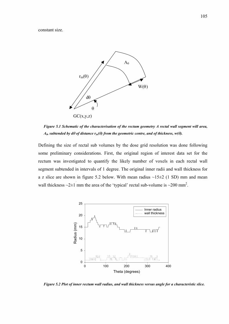
105
constant size.
Figure 5.1 Schematic of the characterisation of the rectum geometry A rectal wall segment will area,
A0, subtended by dθ of distance rin(θ) from the geometric centre, and of thickness, w(θ).
Defining the size of rectal sub volumes by the dose grid resolution was done following
some preliminary considerations. First, the original region of interest data set for the
rectum was investigated to quantify the likely number of voxels in each rectal wall
segment subtended in intervals of 1 degree. The original inner radii and wall thickness for
a z slice are shown in figure 5.2 below. With mean radius ~15±2 (1 SD) mm and mean
wall thickness ~2±1 mm the area of the ‘typical’ rectal sub-volume is ~200 mm2.
GC(x,y,z) θ
A0
rin(θ)
W(θ)
dθ
Theta (degrees)0 100 200 300 400
Rad
ius
(mm
)
0
5
10
15
20
25
Inner radiuswall thickness
Figure 5.2 Plot of inner rectum wall radius, and wall thickness versus angle for a characteristic slice.

106
The subtending angle was selected to be small enough so that the characterisation is
reduced, as close as possible, to 1D along the radius for each subtending angle. The
perimeter of rectal wall included in the typical case above would be ~0.15 mm. Therefore
for some angles, the ray line defining the rectal wall segment area will pass through the
same voxels as adjacent ray lines. This is accommodated by scanning in only one direction
(say, anti-clockwise to be congruent with the figures) and remembering which voxels have
been counted.
The subtending angle of rectal wall sub volumes along the rectum length is used to
construct the DSM. The DSM used in this thesis differs from those mentioned in the
literature (Hoogeman et al 2001, Sanchez-Neito et al 2001). Both of these workers include
the curvature along the length of the rectum. That is, the subtending angle of the rectal wall
is measured perpendicular to the length of the rectum and the surface area is then weighted
according to the vertical angle in that slice. Since this is only a small change we do not
include curvature along the rectal length.
5.3.1.2. Initial Geometry
It is assumed that across patients and treatment fractions, the rectum geometry will be
constant, but the position of GC (geometric centre of the rectum) may vary, and so will the
rectum radius. Clearly, the sample geometry taken from a single CT image will not be
sufficient to model the geometries across the patient population, particularly the size of the
geometry. Thus, to increase the robustness of the rectum geometry, the original rectum
geometry is scaled to conform to the population data accrued by Stroom et al (1999) giving
the initial geometry. The scaling process is done to generalise the size of the rectum
geometry (which might differ substantially from the population mean) following these
steps.
First, the average outer radius (inner radius plus wall thickness) is calculated across all
segments as follows:
( )
360
),(),(0
360
⋅
Θ+Θ=
∑∑=
°
Θ
z
N
zin
N
zwzrr
z
(5.4)
for the number of CT slices, Nz. The population mean radius, popr , from Stroom et al

107
(1999) is then used to derive a scaling factor, poprr , to scale the individual rectum radii in
the original rectum geometry.
5.3.2. Modelling rectum deformations
The MC based method used in the current investigation is similar that used to model the
effect of rigid body translations of the prostate (c.f. §4.3.1). Two steps are modelled for
each patient (planning and treatment delivery). However, at each time interval the rectum
will deform and the geometric centre of rectum will translate. The translation of the
geometric centre needs little explanation because it follows the previously outlined
methods for modelling prostate translations. Thus, this section is dedicated to explaining
the theoretical considerations taken to model rectum deformation
Deformations of the rectum are modelled as changes in rectum radius from the population
mean radius (n.b. all input parameters are discussed in §5.3.5.2). The magnitude of the
inter fraction change in radius is sampled from the distribution of rectum radii (provided in
Stroom et al 1999). A single sampled variable, ζ, is used to deform the entire rectum. Since
the magnitude of the sample change in radius will depend on the initial radius in that
segment of rectum wall a scaling procedure is performed. For inner rectum radius rin(z,θ) a
scaled change in radius, ∆r(z,θ), is calculated from the sampled variable:
Θ⋅=Θ∆
poprzrzr ),(),( ζ (5.5)
Effectively this means that if the rectum radius in a particular z slice is smaller than the
mean radius along the length, the change will be reduced from the sampled change.
Conversely, those sections of rectum wall with radius larger than the mean radius will have
increased change from that sampled value. From examining rectum geometries across
patients in the clinic, it is believed that the scaled change of radius is more accurate than
assuming a uniform change of radius for all z slices. The scaled change of radius will
however be less accurate than methods acknowledging the biomechanics of rectal tissue
that allow each rectal wall segment to be scaled, not only with initial radius but with
adjacent wall segments also (Yan and Lockman, 2001).
Another assumption is that following each change of radius the rectal wall segment area is
kept constant. This infers two main considerations: that the rectal volume is constant, and

108
that the wall thickness of each rectal wall segment will change accordingly. Figure 5.3
demonstrates typical changes of wall thickness implied by the assumption of constant
rectal wall segment area.
1
1.5
2
2.5
3
3.5
6 8 10 12 14 16 18
radius (mm)
wal
l thi
ckne
ss (m
m)
original radius
Figure 5.3 Calculated wall thickness (equation 5.7) with changes of rectal wall radius.
A number of studies in the literature have measured the change in rectum volume (Tait et
al 1993, Melian et al 1997, Pavel et al 2001). Melian et al (1997) show systematic
differences in rectum volume (including contents) of ~50 cm3 between patients and ~30
cm3 between fractions for a single patient. Pavel et al (2001) measured the standard
deviation in rectum volume to be 22% of the original volume. No studies were found in the
literature that measured the inter fraction change in rectal wall volume. In this thesis
constant rectal wall volume is assumed. Wall thickness changes to maintain constant rectal
wall volume.
Figure 5.4 identifies the symbols used to describe changes in rectal wall thickness. The
change in wall thickness, ∆w(z,θ) can be calculated from the original segment area;
( )[ ]20
200 rwrA −+= π (5.6)
Rearranging equation 5.6 and solving the quadratic equation in wall thickness gives:
2000 rArw +±−= π , (5.7)

109
where only the positive root is a physical solution. For deformed radius, rdef, the deformed
wall thickness is then;
200 rArw def ++−=∆ π . (5.8)
where rdef = r0 + ∆r.
A0
∆r
rin
w
r′in = rin + ∆r
w′
thickne
Figure 5.4 Rectum segment has constant area. Dashed segment is original segment.
5.3.3. Modelling planning CT image acquisition
For the purpose of modelling we assume that mean positions of the prostate and rectum as
well as mean rectum radius is known for the patient population. For a single patient, the
rectum position and dimensions at the time of the planning CT acquisition will differ from
the population mean, but the average position and dimensions will be close to that for the
population over an entire fractionated treatment.
The rectum dimensions as imaged in the planning CT scan will differ from the true rectum
dimensions (in a similar way to the prostate position at planning). In each z plane they are
sampled from the radius distribution to vary about the population mean dimensions.
Movements of anterior rectal wall will influence the position of the prostate. We assume
that these movements are correlated. Therefore variance of the rectum radius distribution
combined with that of the geometric centre (GC) of the rectum should sum to the variance

110
of prostate movement. Lateral rectum deformations will not impact on prostate position
and SI deformation is not modelled.
The geometric centre of the rectum will be shifted in the planning CT image from the true
position as mentioned in §3.3.1 for the prostate. Briefly, the position of the mobile organ at
the time of CT imaging will be a sampled position in the distribution of possible organ
positions.
Averaging multiple rectum dimensions and positions from multiple temporally spaced CT
image sets will undoubtedly improve the estimation of the mean rectum dimensions about
the geometric centre of the rectum. Multiple pretreatment imaging to average dimensions
and location is modelled. Clinically, in most cases, the clinician would improve the
definition of CTV following each successive image set acquisition and may use reduced
margins (c.f. equation 4.11).
The initial rectum geometrical data and the pre-calculated dose distribution are placed on a
3D Cartesian grid (see figure 5.5). A shift of the geometric centre of the rectum is done
over the dose grid for the entire organ. Figure 5.5b shows a simple shift of the rectum GC
posteriorly. For the calculation of biological indices in the next chapter (c.f. §6.2.2) the
prostate is assumed to move with the anterior rectal wall contrary to the depiction in figure
5.5b.
Deformation is calculated as a change in radius and requires a separate calculation for each
rectal wall voxel. The rectal wall voxels are mapped by the treatment planning system on a
Cartesian grid. Therefore sampled values of radius need to be related to the GC. The
Cartesian shift is the change in position of a rectal wall voxel from the original (mean)
position in Cartesian units. The Cartesian shift is calculated for each voxel as
laterally, and ( )Θ⋅∆=∆ sinrxdef ( )Θ⋅∆=∆ cosrydef in the AP direction. The deformation
may be generalised by a change to the function defining the location of voxels allocated as
rectal tissue, that is;
( ) ( )zzyyzxxBzyxB defdefdef ),,(),,(,, Θ∆+Θ∆+⇒ (5.9)
The average rectum dimensions, following multiple CT scans, can be calculated as;
( zzyyzxxB CTCTCT ),,(),,( Θ∆+Θ∆+ ) (5.10)

111
where
CT
N
iiCT
CT N
zxzx
CT
∑=
Θ∆=Θ∆ 1
, ),(),( (5.11)
and similarly for the y deformation. Deformation in the z plane is not included in the
model.
10 20 30 40 50
AP
(mm
)
0
10
20
30
40
50
602010
30
30
30
30
30
20
20
20
10
10
10
40
404040
40
40 40
50
505050
50
50 50
60
6060
60
60 60
30
30
30
30
20
20
20
2010
10
10
ata10 20 30 40 50
AP (m
m)
0
10
20
30
40
50
602010
30
30
30
30
30
20
20
20
10
10
10
40
404040
40
40 40
50
505050
50
50 50
60
6060
60
60 60
30
30
30
30
20
20
20
2010
10
10
X DataLateral (mm) X DLateral (mm)
Figure 5.5 Modelling shifts of the rectum GC is done by shifting the entire organ within a fixed dose
grid. a) The rectum GC position in the original CT planning image is compared to b) the position
(shifted posteriorly) in a later fraction, or CT image acquisition.
As mentioned above, the geometric centre of the rectum as shown in the initial planning
CT image will also not reflect the true mean geometric centre. Therefore, the average
geometric centre of the rectum (over a few CT sessions) will have vector co ordinates:
( )zyyxxGC GCGC ,, ∆+∆+ (5.12)
where GCx∆ and GCy∆ are calculated similarly to ξ in equation 3.3 from NCT pretreatment
CT scans to improve localisation precision. The vector describing a shift of the geometric
centre of the rectum will not depend on the z slice or the angle, θ, subtending that rectal
wall segment.
The modelled treatment planning concludes with the sampled mean geometric centre of the
rectum and mean radius (for each z and θ).
112
5.3.4. Modelling treatment delivery
Following each fraction the geometric centre of each transverse rectum slice will be
described by the vector coordinates:
GC(x+∆xgc(z), y+∆ygc(z), z) (5.13)
where ∆xgc(z) and so on reflect a shift of the geometric centre from the original GC due to
random interfraction setup errors and organ motion. The dimensions of the rectum will also
change from the population mean dimensions, following equation 5.9 above, with ∆xdef
due to an interfraction change of rectum radius (deformation). No time trend has been
modelled following a serial CT study in literature (Lebesque et al 1995) demonstrating
constant random rectum wall motion.
To summarise, the dose deposited in each rectum wall segment will depend on the current
position of that wall segment accounting for;
systematic change in the geometric centre (shift), GCx∆ ο
systematic rectum radius error (deformation), ),( θzxCT∆ ο
systematic patient position error (shift), CTx∆ ο
random interfraction changes in the geometric centre (shift), gcx∆ ο
random interfraction changes in the rectum radius (deformation), ),( θzx∆ ο
random patient position error (shift), x∆ . ο
In order to calculate the dose to the voxel of tissue (moving during the treatment) the dose
deposited to the moving voxels will then be translated to the stationary voxels in the
original co ordinate system.
This is the dose collected by the moving voxels through the treatment process. Thus, at
every fraction of the simulated treatment, the dose deposited into rectum voxels will exist
in the dose grid co ordinates, B∈D(x,y,z). This translates to the dose from voxel

113
( ) ( )zzyyxxDzyxD ′+′+′+⇐ ,,,, (5.14)
where the primed variables include all of those uncertainties listed above. Explicitly, this
may be expressed as;
xzxxxzxxx gcCTCTGC ∆+∆+∆+∆+∆+∆=′ ),(),( θθ (5.15a)
yzyyyzyyy gcCTCTGC ∆+∆+∆+∆+∆+∆=′ ),(),( θθ (5.15b)
zzz CT ∆+∆=′ (5.15c)
In equation 5.15 lower case gc has been used to denote that this is an inter-fraction shift of
the geometric centre. The use of capitalised GC is reserved for describing a systematic
shift of the geometric centre. Changes in rectum dimensions will imply different changes
of radius in each z slice and for each rectal wall segment. Therefore, a shift of rectal wall
voxels due to deformation is dependent on z and θ in equation 5.15 above.
Dose is accumulated to rectal wall sub volumes (following equation 5.15) through 30
fractions of treatment. This process is repeated for a population of 1000 patients. Patient
specific data is calculated with set systematic errors to evaluate the effect of full and empty
rectum during the planning CT scan.
5.3.5. The input data
5.3.5.1. Geometry
The original rectum geometry and three planned dose distributions (reflecting three PTV
margins about the same prostate CTV) were accessed from the Pinnacle (v5.2g) TPS. This
particular TPS saves the dose matrix related to each incident beam in an easily located
directory. Parameters relating to the dose matrix including matrix dimensions, grid size,
and origin are saved by the software in a text file. The original rectum geometry is also
saved in a text file. The original rectum geometry is represented as a series of Cartesian co
ordinates. Each co ordinate is defined (in close to real time) as the ROI is being delineated
in each CT slice. A linear interpolation is performed for the case where ROI points are
separated by more than one voxel.

114
5.3.5.2. Uncertainty parameters
From the serial CT study performed by Stroom et al (1999) the parameter values for
rectum size and position variations shown in table 5.1 were taken. The table also shows the
values of patient positioning errors for prostate treatments.
Table 5.1 The parameters defining systematic and random changes in rectum geometry
Uncertainty parameter Value (mm)
Population mean rectum radius, popr , 17.5
Systematic rectum radius standard deviation, Σr 6
Random rectum radius standard deviation, σr 3
Systematic patient position error, ΣSE (LR,AP,SI) 2.4, 2.8, 1.6
Random patient position error, σSE (LR,AP,SI) 2.4, 2.8, 1.6
No statistics on the variability of the geometric centre of the rectum was found and
therefore this parameter was set to zero.
5.3.6. Calculations
The mean and standard deviation in mean dose was calculated for a set of parameters. The
parameters include the number of pretreatment CT scans (reducing the systematic error in
prostate PTV field position), and the planned dose distribution used (reflecting three CTV-
PTV margins). Calculations were performed to model a single patient with specified
systematic error and also to model a population of patients with a sampled range of
systematic errors across the population. For the individual patient calculation, the rectum
radius in the single CT image set was specified to include a systematic error. Two
systematic error values were used.
The first systematic error forced the rectum to be 2 standard deviations (~5.6 mm) larger
than the mean rectum wall radius in the planning CT scan to model a full rectum at
planning. This type of systematic error will force the sampled changes of radius (during the
course of treatment) to be reduced from that in the planning CT image. The sampled
changes of rectum radius will be symmetrical about the mean position. However, during

115
treatment delivery the rectum will tend to be further from the PTV.
The second systematic error conversely forces the rectum to be 2 standard deviations
smaller than the mean rectum wall radius in the planning CT scan to model an empty
rectum at planning.
The mean DSH is calculated using:
( ) ( )∑=
=txN
i tx
i
NdDSH
dHSD1
(5.16)
where DSHi(d) is the surface area taken to at least dose, d, for the ith patient.
The mean and standard deviation in the mean dose surface map are calculated for each
rectal wall voxel. Each voxel is a segment on the interior rectal wall with location given by
the subtended angle (refer to figure 5.1) and rectal wall length (increasing superiorly).
5.4. Results
5.4.1. Planned rectum dose distributions
The planned rectum dose distribution for each of the margins are summarised as dose
surface histograms in figure 5.6, and dose surface maps in figure 5.7.
0
20
40
60
80
100
0 10 20 30 40 50 60
Dose (Gy)
5 mm10 mm15 mm
Figure 5.6 Dose surface histograms of the planned dose distributions with CTV-PTV margins of 5, 10,
or 15 mm.

116
r
Figur
10 mm
a)
r30-40 Gy
40-50 Gy
50-55 Gy
55-58 Gy
b)58-60 Gy
>60 Gy
r
c)e 5.7 Dose Surface maps of the planne
, or c) 15 mm. Orientation: Left=0°; A
Superio
d
Superio
d
nt
Superio
ose distributions with CTV-PTV margins of a) 5 mm, b)
erior=90°.

117
5.4.2. Interfraction variations
The interfraction rectal wall deformations were simulated with a set systematic error and
random interfraction errors. Two main cases were simulated: a patient with empty rectum
at planning and a patient with full rectum at planning.
5.4.2.1. Systematic error: empty rectum at planning
The systematic error caused by an empty rectum at planning was modelled by setting the
rectum radius decreased from the mean rectum radius. The set of dose surface histograms
comparing the planned dose distribution, for each margin size, with the calculated mean
dose distribution incorporating both the systematic and random errors is given in figure 5.8
below.
0
10
20
30
40
50
60
70
80
90
100
0 10 20 30 40 50 60
Dose (Gy)
5 mm Mean10 mm Mean15 mm Mean5 mm Plan10 mm Plan15 mm Plan
Figure 5.8 DSH showing the mean and planned dose distributions modelling an empty rectum at
planning with three CTV-PTV margins.
Figure 5.8 shows two major trends; the percentage of rectal surface area receiving dose
greater than ~32 Gy (53% of target dose) is generally increased from that planned, and the
percentage of rectal surface area receiving dose less than ~32 Gy in generally reduced from
that planned. This confirms the trend that an empty rectum at planning will generally shift
the rectum into the PTV. The difference between the mean and planned dose is greatest

118
with the 5 mm margin. For example, the lowest planned dose with a 5 mm margin is ~28
Gy, but the lowest mean dose is ~10 Gy. Also the mean dose to 20% of the rectal wall is
increased by ~7 Gy from the plan.
The difference between the planned dose and mean dose (i.e. D0- D ) is plotted in figure
5.9 below as dose surface maps for each margin size. These maps enable visualisation of
the location of dose difference. In each of the dose surface maps the black sections infer
that the range of values signified by colours has been exceeded. The mean dose is
increased from the planned dose where D0- D < 0. The range of difference values (i.e. D0-
D ) reduces as the margin is increased, from -20 Gy to 22 Gy with the 5 mm margin to -18
to 7 for the 15 mm margin. This indicates reduced stability with the smaller margin.
With a 5 mm margin the increase in dose generally occurs in the inferior anterior rectal
wall, with some portions receiving greater than 15 Gy below the planned dose. The
reductions in dose generally occur in the posterior lateral wall coinciding with the PTV
(i.e. the middle slices superiorly). The mean dose is reduced from the planned dose in some
portions of the rectal wall by as much 15 Gy. However, over 60% of the rectal wall surface
area has a mean dose within 5% of the planned dose.
With a 10 mm margin the increase in dose occurs in the inferior anterior rectal wall. The
reductions in dose occur mainly in the right lateral wall. The largest increase in dose is
greater than 15 Gy above the plan, while the largest decrease is less than 10 Gy below the
plan. The 10 mm margin has greater than 85% of the rectal wall surface area within 5 Gy
of the planned dose.
With a 15 mm margin the increase in dose occurs in the inferior anterior lateral rectal wall,
with some small portions receiving greater than 15 Gy above the planned dose. Dose
reductions are present in the anterior and posterior rectal wall; however, the maximum
reduction in dose is only 5 Gy. The proportion of rectal wall receiving a mean dose
relatively indiscriminate from the planned dose is about 95% of the surface area. Thus as
the PTV in increased the effect of this systematic error (i.e. an empty rectum at planning) is
reduced.

119
r
D
r
Figure 5.9 Dose Surface Maps showing th
distributions with empty rectum at planning
Orientation: Left=0°; Anterior=90°.
Superio
-15 - -5 Gy
-5 - 0 Gy
0 - 5 Gy
5 - 10 Gy
10 - 15 Gy
>15 Gy
r
e
fo
Superio
Superio
difference between planned and delivered r
r a) 5 mm margin, b) 10 mm margin, c) 15 mm
D0-
ectal dose
margin.
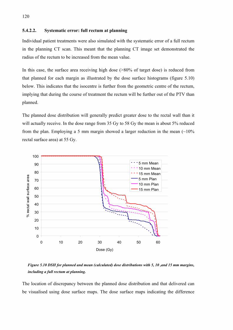
120
5.4.2.2. Systematic error: full rectum at planning
Individual patient treatments were also simulated with the systematic error of a full rectum
in the planning CT scan. This meant that the planning CT image set demonstrated the
radius of the rectum to be increased from the mean value.
In this case, the surface area receiving high dose (>80% of target dose) is reduced from
that planned for each margin as illustrated by the dose surface histograms (figure 5.10)
below. This indicates that the isocentre is further from the geometric centre of the rectum,
implying that during the course of treatment the rectum will be further out of the PTV than
planned.
The planned dose distribution will generally predict greater dose to the rectal wall than it
will actually receive. In the dose range from 35 Gy to 58 Gy the mean is about 5% reduced
from the plan. Employing a 5 mm margin showed a larger reduction in the mean (~10%
rectal surface area) at 55 Gy.
0
10
20
30
40
50
60
70
80
90
100
0 10 20 30 40 50 60
Dose (Gy)
5 mm Mean10 mm Mean15 mm Mean5 mm Plan10 mm Plan15 mm Plan
Figure 5.10 DSH for planned and mean (calculated) dose distributions with 5, 10 ,and 15 mm margins,
including a full rectum at planning.
The location of discrepancy between the planned dose distribution and that delivered can
be visualised using dose surface maps. The dose surface maps indicating the difference

121
between planned and mean delivered dose is illustrated in figure 5.11 (below) for each
margin size.
Employing a 5 mm margin will cause an increase in the dose to the posterior rectal walls
that is generally less than 2 Gy from the planned dose. Decreases in dose, as large as 16 Gy
below that planned, occur in the lower anterior rectal wall. Despite this large magnitude of
dose reduction, approximately 90% of rectal surface area will be within 5 Gy of the plan.
The mean rectal dose with a 10 mm margin shows increases in the posterior lateral walls of
less than 2 Gy from the plan. The decreases in dose occur in the mid anterior wall, with
deviations as large as 12 Gy below the plan. Approximately 85% of the rectal wall shows a
mean dose that is relatively (i.e. < 5 Gy) unchanged from the plan.
With a 15 mm margin, a small increase (< 2 Gy) is present in the posterior lateral rectal
walls. A decrease in dose is present in the lower inferior rectal and inferior portions of the
lateral rectal walls. As with the other margin sizes, approximately 90% of the rectal surface
area was with in 5 Gy of the planned dose. Therefore this systematic error (i.e. full rectal at
planning) appears to be relatively unaffected by the size of the PTV.
5.4.3. Interpatient variations
Across a population of patients a range of systematic errors will occur additional to the
random errors. Figure 5.12 illustrates the rectal wall dose surface histograms from 20
sampled treatments including both systematic and random errors across the population
(dashed curves) for each margin size tested. The planned rectal wall dose surface
histograms for each margin are also shown (solid curves). The dose surface histograms in
figure 5.12 include the extreme outcomes indicated in the previous section (c.f. figures 5.8
and 5.10) with fixed systematic errors (and possibly beyond) as well as many outcomes in
between.
The mean rectal dose for each patient does not change significantly across the population.
Furthermore, the planned and the mean dose distributions calculated with only one
pretreatment CT scan are almost equivalent. This is due to the use of normal distribution
for sampling systematic error combined with limiting the potential increase of the rectal
wall diameter to the physical diameter of the pelvic inlet (which did not change between
modeled patients since only one patient image was used).

122
r
Figur
15 mm
a)
D r
-2 - 0 Gy
0 - 4 Gy
b)4 - 8 Gy
8 - 12 Gy
12 - 16 Gy
> 16 Gy
r
c)e 5.11 DSM showing where the differen
with full rectum at planning. Orientat
Superio
c
io
Superio
Superio
e dose occurs for margins of a) 5 mm, b) 10
n: Left=0°; Anterior=90°.
D0-
mm, and c)

123
The number of CT images would, of course, affect the standard deviation in the mean
rectum position. As this number, NCT, increases the standard deviation would be reduced
as ~CTN
1 . Consequently, the number of pretreatment CT scans did not affect mean
rectal dose. Therefore in this section the term, mean dose, will imply that a single
pretreatment CT scan was used for planning purposes.
Despite the similarity between the mean inter-patient rectal doses, for all margins tested,
significant differences did occur in the rectum dose for individual patients. This is reflected
in the standard deviation in mean rectal wall dose (see figures 5.13, 5.14 and 5.15 below).
For the 5 mm and 10 mm margins, a large SD in dose did occur at three locations in the
rectal wall, including; length-wise along the anterior lateral wall, in the lower anterior
inferior wall, and in the middle (superiorly) of the right lateral wall. These locations lie in
regions of dose gradient (c.f. planned DSMs in figure 5.7 above). Employing a 5 mm
margin the anterior lateral wall of the rectum is positioned in the planned lateral penumbra
of the dose distribution. The inferior portion of the anterior rectal wall is positioned in the
planned inferior penumbra. The inferior portion of the rectal wall (below the 4th CT slice)
has a smaller radius than the superior portion. The highly variable dose at 190°
corresponds to the left lateral wall (approximately slice 5) where the planned dose is below
30 Gy due to the posterior and lateral distance from the prostate. The opposing (right)
lateral rectum wall received a higher dose indicating that the rectum is not centred laterally
in the field.
With the 10 mm margin, the interpatient dose difference in the left lateral wall was
removed by averaging just 2 pretreatment CT scans. The left lateral wall has a higher
planned dose with the 10 mm margin than with the 5 mm margin. Even with infinite
pretreatment CT scans the variation in inferior anterior wall is greater than 2 Gy and the
surface area with dose SD greater than 1 Gy extends along the anterior lateral wall aswell.
With the 15 mm margin the SD in dose is noticeably shifted posteriorly compared to the
smaller margins (c.f. figures 5.13 and 5.14 above). The high dose surface area is increased
in the inferior portion of the anterior rectal wall, and a band of SD (not present with
smaller margins) occurs in the superior portion of the rectal wall. With a 15 mm margin the
superior rectal wall is positioned in the superior-posterior dose gradient. As the margin size
is reduced the dose gradient shifts inferiorly, away from the posterior rectal wall.
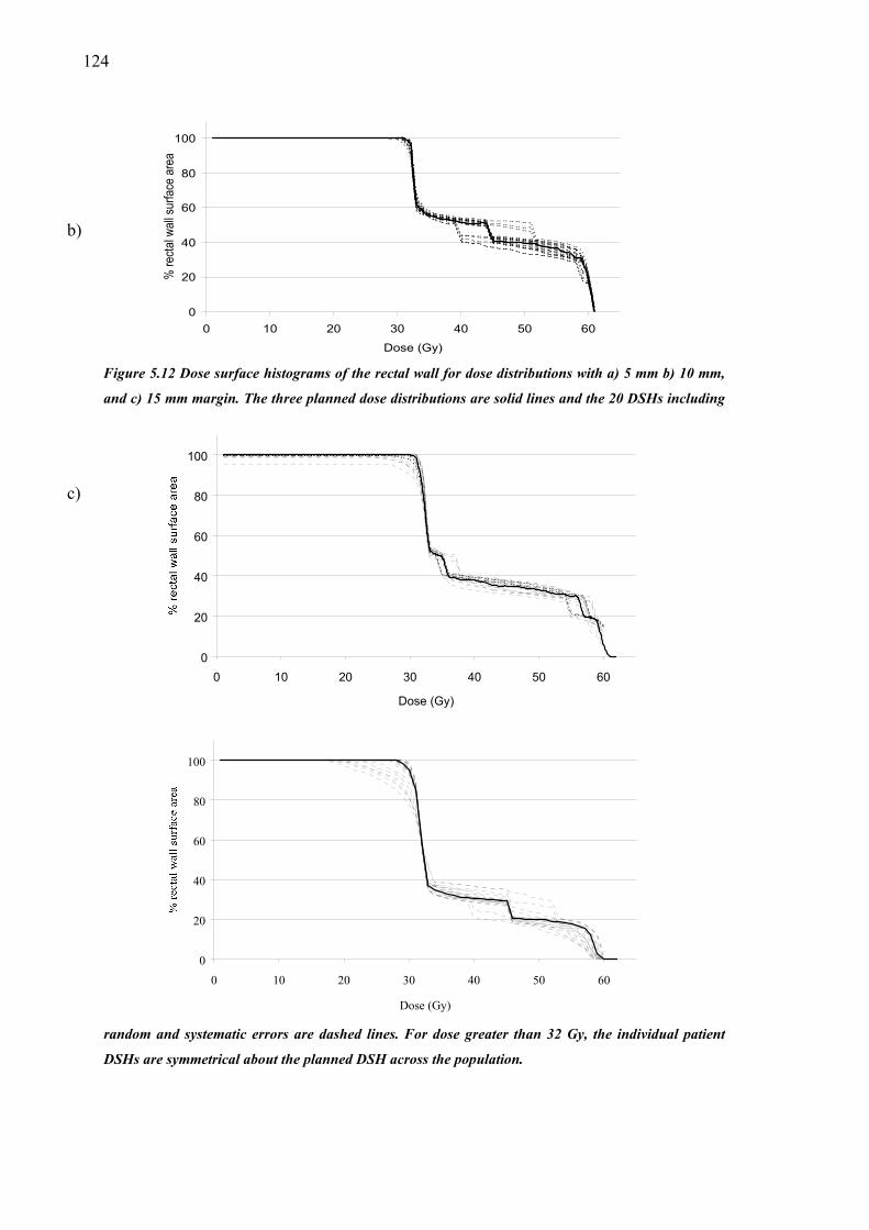
1
24
0
20
40
60
80
100
0 10 20 30 40 50 60
Dose (Gy)
% re
ctal
wal
l sur
face
are
a
Figure 5.12 Dose surface histograms of the rectal wall for dose distributions with a) 5 mm b) 10 mm,
and c) 15 mm margin. The three planned dose distributions are solid lines and the 20 DSHs including
60
80
100
b)
c)
random and systematic errors are dashed lines. For dose greater than 32 Gy, the individual patient
DSHs are symmetrical about the planned DSH across the population.
0
20
40
0 10 20 30 40 50 60
Dose (Gy)
0
20
40
60
80
100
0 10 20 30 40 50 60
Dose (Gy)

125
Figure
pretreat
Orienta
a)
r SD, ΣD
1-2 Gy
2-3 Gy
b)3-4 Gy
4-5 Gy
5-6 Gy
>6 Gy
r
c)5.13 The standard deviation in rect
ment CT scan with, b) two pretreat
tion: Left=0°; Anterior=90°.
Superior
al
me
Superio
Superio
wall dose calculated with 5 mm margin and a) one
nt CT scans, and c) infinite pretreatment CT scans.
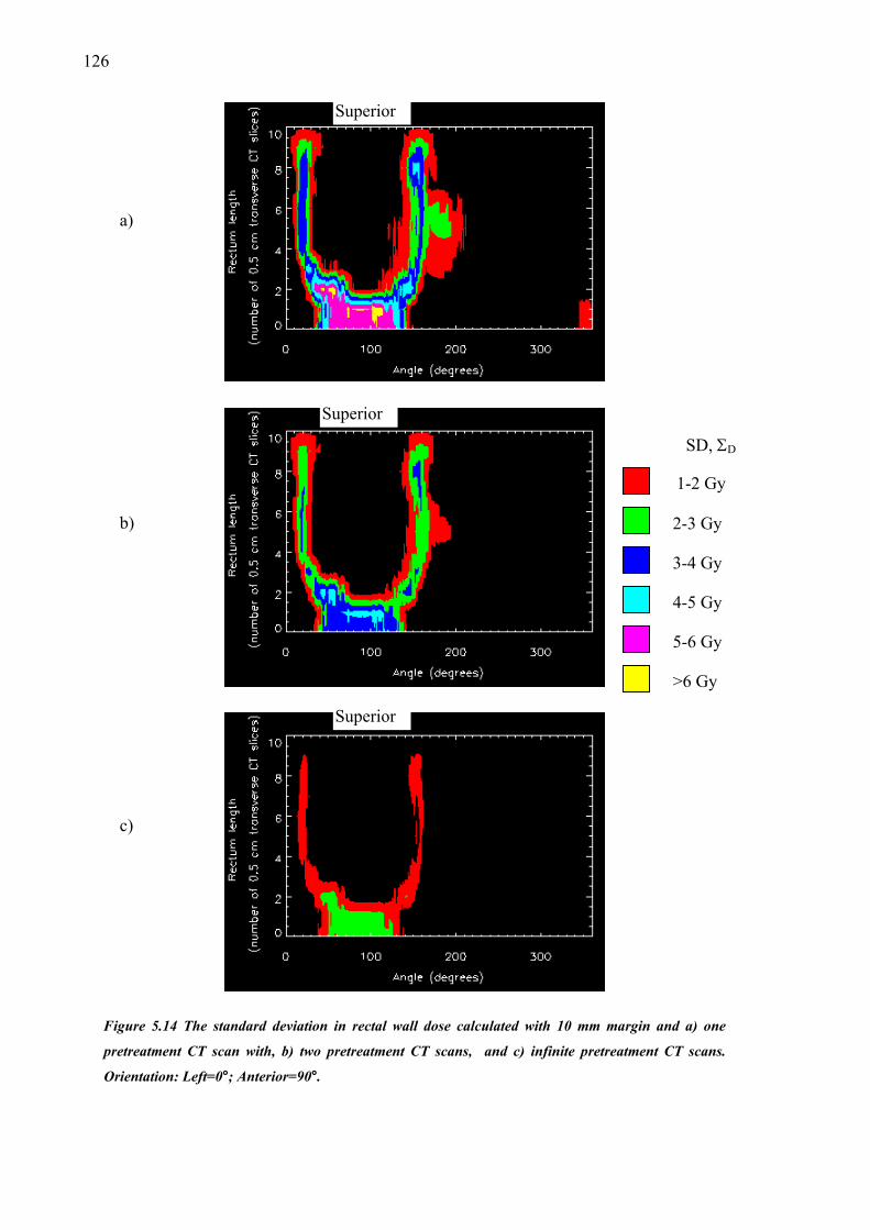
126
r
)
F
p
O
a
r
SD, ΣD
1-2 Gy
2-3 Gy
b)3-4 Gy
4-5 Gy
5-6 Gy
>6 Gy
r
c)igure 5.14 The standard deviation
retreatment CT scan with, b) two p
rientation: Left=0°; Anterior=90°.
Superio
Superio
Superio
in rectal wall dose calculated with 10 mm margin and a) one
retreatment CT scans, and c) infinite pretreatment CT scans.

127
r
Figur
one, b
Anter
a)
r
SD, ΣD
1-2 Gy
2-3 Gy
3-4 Gy
b)4-5 Gy
5-6 Gy
>6 Gy
r
c)e 5.15 The standard deviation in dos
) two, and c) an ‘infinite’ number o
ior=90°.
Superio
Superio
Superio
e presented as a DSM. A margin of 15 mm is used with a)
f pretreatment CT scan information. Orientation: Left=0°;

128
5.5. Discussion
The rectum will deform during treatment and this has been shown to impact on the
individual patient and the population averaged dose distributions. The size of the margin is
naturally of fundamental importance. Three margin sizes were modelled, and as the size of
the margin was increased the rectal wall surface area receiving high dose increased.
For an individual patient with empty rectum at planning, the PTV will be placed closer to
the position of the mean anterior rectal wall. The dose surface map shows increases in the
surface area receiving high dose (greater than ~50% target dose) from that planned and
lower percentages of surface area receiving low doses (less than ~50% target dose). For the
smallest margin size (5 mm) the reduction in surface area receiving low doses is markedly
greater than for the large margin size (15 mm). The mean dose surface maps show that the
posterior penumbra is shifted posteriorly, in a similar way to increasing the margin size.
For an individual patient with full rectum at planning, the field will, predominantly, be
placed further from the mean anterior rectal wall position. The DSH shows decreases in the
surface area receiving high dose (greater than ~30 Gy), the maximum dose is reduced
while the surface area receiving low dose (less than ~30 Gy) is marginally larger. The
amount of surface area reduction at the higher doses is greater for the smaller margin. The
mean dose surface maps show that for the 5 mm margin the posterior penumbra is brought
anteriorly into the anterior rectum wall. The mean dose is deposited anterior to the plan for
the other margin sizes as well. For the 15 mm margin this causes the superior border of
rectal wall data set to interact with the superior-posterior penumbra.
With the simulated full rectum at planning systematic error, the difference between
planned and mean dose was demonstrated with dose surface maps and appeared to be
independent of the PTV. With each margin size about 90% of the rectal surface area was
less than 5 Gy from the planned dose. However, the simulated empty rectum at planning
indicated that the (relatively) unaffected fraction of rectal surface area increased from
~60% with a 5 mm margin to ~95% with a 15 mm margin.
The interpatient results show that mean dose to rectum will not be significantly different
from the planned dose across a patient population. This follows directly from the
assumption of a (symmetrical) Gaussian PDF to describe interpatient variation. Reduction

129
in the variability of rectal dose received occurs when the organ position is averaged across
multiple pretreatment CT image sets, particularly with the smaller (5 mm) margin. The
reduction in dose occurred in the areas of the rectal wall (from the planning CT) that
coincide with planned dose gradient. The use of multiple pretreatment CT images further
reduced this effect. Major benefit for the 5 mm margin was calculated for the anterior
lateral wall, inferior anterior wall and a section on the left side of the lateral wall. The
initial effect from sampling rectal wall position with one CT image was reduced with the
10 mm margin. With the 15 mm margin, the major location of interpatient variability in
dose was a band around the superior portion of the rectal wall, but this reduced
substantially with the use of information from multiple CT image sets.
The modelling of rectum deformation in this Chapter has a number of critical assumptions
that impact on the results. Firstly, the interfraction variation in rectal wall radius is initiated
from a single sampled variable, constraining the geometry in each transverse CT slice. This
produces uniformity in motion along the length of the rectum that may not be present
naturally. The alternative is to use a database of possible geometries and sample variations
amongst and between those present in that database. However, in that case, much more
data would need to be collected. In any case, the local deformations in the rectal wall
shouldn’t produce more than small areas of increased exposure (surface area) to target
dose. Considering these factors, the current technique is still a good approximation and
should give relatively sound and accurate results.
Secondly, the original data set may not be representative of the rectum geometry or size for
the patient population. The first order approximation used included scaling this original
geometry according to a measured distribution of inter-patient mean rectum diameters.
While higher order techniques would produce more accurate modelling, the effect on dose
is expected to be small.
Lastly, the changes in rectum radius were modelled about the geometric centre of the
rectum. The model was developed to incorporate motion of the geometric centre, but no
data was found in the literature and it would be a difficult (and not otherwise useful)
parameter to measure. To some extent, motion of the geometric centre of the rectum was
included in (and probably over compensated for by) the parameters defining motion of the
rectal wall.
130
Clearly, a model incorporating mechanical data on the rectal tissues (such as described
above, see §5.2) would produce meaningful generalised information on movement from a
small number of measured parameters (Yan and Lockman 2001). That is, by measuring a
fixed number of displacement vectors (tracking movement of labelled rectal wall voxels)
further displacement vectors might be calculated based on the tissue properties. In this
way, the ART process is made less labour intensive and more eloquent. It is important and
useful to study the effect on rectal wall dose from those uncertainties present in current
clinical practise.
This chapter investigated more comprehensive modelling of rectal wall deposition than
that presented in the previous chapter. The rectum will change radius during treatment, and
thus rectal wall tissue will displace towards, away, and laterally to the high dose target
volume (respectively, in the case of rectum expansion for the anterior, posterior and lateral
walls). Therefore, the assumption of linear translations of the whole rectum, such as has
been described of the prostate is obviously an over-simplification.
The rectum has been included in many clinical studies of tolerance doses because of it’s
proximity to the prostate, the high incidence of prostate cancer amongst men worldwide,
and the implementation of techniques of IMRT used with dose escalation to treat the
disease. A 60 Gy treatment was modelled in this chapter, however, in the current climate
many centres may be treating to higher doses, as high as 90 Gy and potentially higher.
Those centres treating to high dose will probably be using a more tightly conforming dose
volume than the dose distribution created by a four field box technique. The results
presented are dependent on the technique (mechanical dose delivery and dose
computation) as well as the maximum dose. With sharper dose gradients a larger variation
in dose will occur. Further study may be useful for a range of dose distributions (other than
margin size differences) and a range of target doses.
5.6. Conclusions
The model of interfraction rectal wall motion studied in this chapter produced knowledge
of the most probable dose deposited in rectal wall tissue.
Individual patients with treatments designed using a CT image set where the rectum is
larger than average will receive substantial reductions in mean dose from that planned. The
131
largest effect will be with a 5 mm margin.
Conversely, those individual patients with treatments designed using a CT image set where
the rectum is smaller than average may receive larger areas of rectal wall with high dose.
Again the plan with a 5 mm margin is more sensitive to dose variation than the plans with
larger margins.
Across a population of patients, a Gaussian interpatient systematic error, will not largely
affect the mean rectal dose. However, the inter-patient variation in rectal dose will be
significant. For the 5 mm margin, the major dose uncertainty occurred in the anterior
lateral rectal wall, the inferior anterior wall, and (for the chosen case) in the left lateral
wall. The later dose uncertainty occurred due to the particular geometry dictating that the
left lateral rectal wall was lateral to the lateral penumbra. The averaging of rectal position
in multiple pretreatment CT scans reduced the variability in delivered dose across the
population for this margin. For the 10 mm and 15 mm margins, averaging rectal position
from extra pretreatment CT scans did not have as marked an effect as for the 5 mm margin.
The position of dose gradient (posterior penumbra) moves posteriorly as the margin is
increased. Thus, for the 10 mm margin, the size of the left lateral wall dose variation is
reduced. The posterior location of the dose uncertainty is present further posteriorly with
the 15 mm margin and the superior limit of the rectal wall data set begins to be affected by
the superior-posterior penumbra.
Overall, the individual patient may receive up to 15 Gy (i.e. 25% of target dose) above or
below that planned depending on the rectal geometry in the planning CT image set. The
majority of dose uncertainty occurs in the lateral rectal walls and therefore the change in
high dose volume (i.e. that volume receiving >80% CTV dose) is not significantly variable.

132

133
Chapter 6
Modelling the radiobiological effect of
treatment uncertainty in radiotherapy
6.1. Introduction
The treatment of prostate carcinoma with external beam radiotherapy is performed with
knowledge of treatment uncertainties. Consequently, a margin is selected that encompasses
the tumour and ensures full (prescription) dose is given to the diseased tissue. As
investigated in previous chapters, due to the treatment uncertainties, the dose deposited in
the prostate gland and rectal wall will vary between fractions for individual patients, and
will vary between patients across the treated population.
This chapter investigates the effect on Tumour Control Probability (TCP), Normal Tissue
Complication Probability (NTCP) and Uncomplicated Tumour Control Probability (UTCP)
from the uncertainty in delivered dose, and radiosensitivity.
6.2. Tumour Control Probability
The tumour control probability is the probability of completely eradicating all clonogens
from the local tumour site. Much work has been done to characterise the survival of
patients with prostate carcinoma following irradiation as previously outlined (c.f. §3.3).
In this section, two TCP investigations were done; 1D and 3D. The one dimensional case
examined the broad context of the biological effect of the treatment errors. The 3

134
dimenional case examined a population of simulated prostate treatments, with feasible
parameter values to investigate the best estimate of clinical impact from the treatment
uncertainties.
6.2.1. Background
Interfraction movements of the prostate and beam will cause the delivered prostate dose to
vary from that planned. The variations in dose delivered will impact on the individual’s
TCP, the mean TCP across the population and the standard deviation in mean TCP across
the population. Brahme (1984) noted that small cold spots of low dose will drastically
reduce tumour control. Conversely boosting a volume within the tumour has been shown to
increase TCP by a relatively small amount. These are direct consequences of the form of
the relationship between TCP and dose predicted by the models. As shown by the
investigation into dose uncertainty done in this thesis, most dose uncertainty occurs at the
beam edges. Current treatment planning techniques acknowledge this by ensuring a safety
margin between the tumour and treated volume.
In 1988, Boyer and Schultheiss evaluated the impact of dose uncertainty using a
convolution of TCP with a Gaussian function in dose. Clearly the use of a Gaussian dose
PDF ignores the radial dose variation (σD(r)) previously derived (refer to §4.2.2). This
chapter will investigate effects of these dose variations, as well as interpatient
radiosensitivity variation, on tumour control.
6.2.2. Method
Tumour control probability is first calculated with a 1D dose profile and then a more
detailed and (clinically) accurate calculation is performed. In this simulation a tumour and
treatment field are both assumed to be spherical. Therefore the single dimension represents
the radius of a sphere centred on a tumour. The 1D dose profile is used to investigate the
impact of three separated issues; prostate motion combined with patient positioning error
(spatially non uniform dose error), spatially uniform dose error, and inter-patient variation
in tumour radio sensitivity. These three issues were simulated using field margins equal to
0.5 cm, 1.0 cm, and 1.5 cm.
Tumour control probability for the nth patient is calculated using (Webb and Nahum
1993):

135
[ ].),,,()()(exp0
∏=
=
⋅⋅−=Xx
xntn xDSxVxTCP βαρ (6.1)
with clonogen density, ρ(x), partial volume of annuli, vt(x), and the surviving fraction of
the nth patient, Sn is dependent on the total dose deposited in tumour tissue, D, the tumour
radio-sensitivity, α, and fractionation factor, β. The impact of three issues that contribute
to uncertainty in tumour control is investigated.
For the spatially non uniform dose errors, the (laterally shifting) fraction dose is
accumulated in tumour voxels (c.f. §4.3). The fraction dose for an individual’s treatment is
shifted laterally from the position planned for delivery. Thus, the fraction dose delivered to
a voxel positioned a distance, ∆x, from the planned position, x0, is given as:
di(x) = d0(x0 + ∆x(σTD) (6.2)
where ∆x is the shift sampled from the treatment uncertainty distribution with standard
deviation, σTD. The treatment uncertainty distribution describes position variations of the
tumour relative to the incident fluence and has variance equal to the sum of the patient
positioning error variance and the prostate motion variance (refer to equation 4.2).
The systematic impact of prostate motion due to use of a single CT image can be reduced
by averaging tumour position from a number of pretreatment CT scans. Thus, the random
position of the prostate (centre of mass) relative to bony anatomy is sampled from the
prostate position distribution a number of times, and the average position is used to
position the planned dose distribution.
For the spatially uniform dose error (c.f. §4.3) the fractional treatment dose, di, is perturbed
from the planned dose giving:
di* = d0 + ∆di(σd) (6.3)
where d0 is the planned fraction dose and ∆di is the sampled dose variation for the ith
fraction. The magnitude of the dose variation at each fraction is sampled from a (Gaussian)
distribution with standard deviation, σd, equal to either 4 cGy (2%) or 10 cGy (5%) for
each 200 cGy fraction.
Variation in patient tumour radio sensitivity across the patient population is modelled by
sampling the individual’s tumour radio sensitivity from the (Gaussian) population

136
distribution. Tumour control probability for the nth individual is then calculated with
radio sensitivity given as;
αn = α0 + ∆αn(σα), (6.4)
where the planned (or expected) cell sensitivity, α0, is varied for that patient by ∆αn, which
will be dependent on the standard deviation, σα, of the population distribution of radio
sensitivities.
The impact of each of these issues is investigated in 1D with three dose profiles describing
CTV margins of 0.5 cm, 1.0 cm and 1.5 cm.
Following the initial 1D investigation of the role and relative impact of each issue on TCP,
a thorough 3D investigation was performed. The 3D case includes accurate geometrical
description of the tumour volume, dose distribution, and tumour characteristics. TCP is
calculated for both the individual (with set systematic error), and across a patient
population. The population results are described by a mean TCP and the standard deviation
in mean TCP.
6.2.2.1. Input data for 1D case
In one dimension, the dose distribution is described by a dose profile. This dose profile is
achieved by averaging the steepest (oblique) and shallowest (horizontal) dose gradients
from the four field box dose distribution. A representative dose distribution is shown in
figure 6.1 below with straight lines indicating the profile orientations.
From the dose profile, the tumour plus CTV-PTV margin was assumed to occupy the space
from the centre to the 95% isodose (see figure 6.2 below). This is in accordance with
current treatment planning techniques that define the PTV before calculating the dose
distribution.
Prostate volume was taken as a sphere with radius equal to the tumour radius. The original
dose profile with a 1.5 cm margin was modified to dose profiles with smaller margins of
0.5 cm and 1.0 cm by deleting the central portion of the original profile. In this way the
penumbra gradient is unchanged.

137
Figure 6.1 Isodose contours for typical prostate treatment. The CTV (solid and filled), PTV (dotted), and rectum (brown) are shown, with the oblique and horizontal lines indicating the position of dose profiles used.
0
20
40
60
80
100
0 1 2 3 4 5 6 7 8
Distance (cm)
CTV5 mm
10 mm
15 mm
Figure 6.2 The dose distribution for 1D TCP calculations.
The prescribed dose to the isocentre is 60 Gy in 30 fractions over 5 weeks. The parameters
used for modelling treatment uncertainties are given in table 4.1 with the exception of
tumour radio sensitivity. No account for tumour repair or repopulation during this
theoretical treatment is taken. The tumour has arbitrary volume 165 cm3 (corresponding to
X Data10 20 30 40 50
AP (m
m)
0
10
20
30
40
50
602010
30
30
30
30
30
20
20
20
10
10
10
40
404040
40
40 40
50
505050
50
50 50
60
6060
60
60 60
30
30
30
30
20
20
20
2010
10
10
Lateral (mm)

138
a radius of 3.4 cm), with clonogen density within the GTV of 107 cm-1 and LQ model
parameters α = 0.35 Gy-1, β = 0.035 Gy-2. Webb and Nahum (1993) fitted this value of cell
sensitivity (α) to laboratory data for bladder cell survival and computed the required
interpatient variation to be 0.08 Gy-1 (1 SD). Intratumour and inter-fraction variation in cell
sensitivity are not included in the calculations.
6.2.2.2. Input data for 3D case
The prostate geometry, dose distribution and dose grid parameters were all accessed from
Pinnacle3 TPS. The prostate geometry included the vector coordinates of a clinican
outlined prostate region of interest in each transverse CT slice. The dose grid matched the
superior-inferior positioning and spacing of the CT slices, and therefore coincided with the
prostate geometry reference frame.
The prostate is considered to be constructed of prostate subvolumes (or voxels). The AP
and lateral dimensions of each subvolume is defined by the dose grid, and the SI
dimensions are defined by the CT slice thickness.
As with the 1D case (above) the parameter values for treatment uncertainty are given in
table 4.1, with the exception of the interpatient radio sensitivity. The current literature
describes the prostate (c.f. §3.3.3) by α = 0.29 ± 0.08 Gy-1 (Sanchez-Neito et al 2001b).
This value was used in the following calculations. The value of β used was calculated for
each patient using a fixed α/β ratio of 10 and their (sampled) α value.
6.2.2.3. Calculations
Tumour control probability is calculated with sample surviving fraction based on the linear
quadratic (LQ) formalism (Fowler, 1989). Surviving fraction for the prostate sub volume at
vector position, x, following an N fraction treatment is computed using equation 6.1
(above).
A Monte Carlo method was used to randomly sample dose as specified in equations 6.2 to
6.4. This was done for a population of 5×10⁴ patients. Distributions of treatment dose were
calculated for the population and used to compute the mean and variance of the treatment
dose. TCP values were calculated for each patient from the population and then
distributions of patient TCP were used to compute mean, mode and variance of the
population TCP.

139
6.2.3. Results
Tumour control probability is presented using 1D and then 3D input data. The 1D
investigation explores the impact of margin size, penumbra steepness and the number of
pre-treatment CT scans with spatially non uniform dose uncertainty, and then investigates
the impact of spatially uniform dose uncertainty and the inter-patient tumour radio-
sensitivity. The 3D investigation follows with the inclusion of spatially uniform and non-
uniform as well as inter-patient cell sensitivity heterogeneity with three margins in the
calculation of mean TCP. These calculations include multiple pretreatment CT scans. The
3D data is also used to calculate the effect of certain systematic errors on TCP for the
individual patient.
6.2.3.1. Impact of margin size
Calculations were performed using the 1D dose profile with margins of 0.5 cm, 1.0 cm,
and 1.5 cm, and with a fixed magnitude of simulated treatment error. The planned dose
distributions are shown in figure 6.2. The dose distributions with margins of 1.0 cm or 1.5
cm are planned to deposit 100% of prescription dose to the CTV, while the dose
distribution with 0.5 cm margin will have slight penumbra in the edges of the planned
CTV. In this case, the minimum planned CTV dose is 98% of prescription dose.
The mean TCP across a patient population is illustrated in table 6.1 and figure 6.3 below.
The magnitude of the decrease in TCP from that calculated with the planned dose
distribution is negligible for the population if CTV-PTV margins of 1.0 cm or greater are
used. With the 0.5 cm margin, the reduction in TCP from the plan (at 60 Gy) is 0.07, and
the surrogate loss of dose at planned TCP values of 0.5 and 0.8 are 0.7 Gy, and 1.4 Gy,
respectively. The reduction in TCP indicates a shift of the mean TCP to higher dose, while
the different loss of dose values at each planned TCP indicates that the slope of the mean
TCP is also reduced from that planned.
The mean TCP calculated with 1.0 cm and 1.5 cm margins were very close (<1%) to the
planned TCP. Similarly, for these margin sizes, the difference between the mode TCP and
the plan was also small (<1%). Accordingly, improving the systematic positioning
accuracy did not affect the mean or mode TCP for these margin sizes. However, the
calculation of mean TCP with a 5 mm margin around the CTV was sensitive to systematic
error.

140
0.0
0.1
0.2
0.3
0.4
0.5
0.6
0.7
0.8
0.9
1.0
40 45 50 55 60 65 70
Dose (Gy)
5 mm plan5 mm 1 CT10 mm plan10 mm 1 CT15 mm plan15 mm 1 CT
Figure 6.3 TCP calculated with planned dose distribution versus mean calculated with CTV-PTV margins of 0.5 cm, 1.0 cm and 1.5 cm (incorporating treatment uncertainty). The magnitude of treatment uncertainty is fixed for all cases.
Table 6.1 The effect of margin size on TCP incorporating treatment uncertainty. The difference between planned TCP and mean TCP with 1 CT (in percentage points), as well as the difference in TCP between the planned and calculated mean TCP are shown.
Margin (cm) ∆TCPD=60 Gy ∆DTCP=0.5 (Gy) ∆DTCP=0.8 (Gy)
0.5 7% 1.4 0.7
1.0 1% 0.4 0.5
1.5 <1% 0.04 0.05
To reduce the systematic component of prostate motion error, a number of organ locations
may be averaged from pretreatment CT scans. Since the standard treatment will rely on a
single pretreatment CT scan the nomenclature of mean and mode TCP will imply that this
is the case, unless otherwise stated. The TCP calculated with the planned (or intended)
dose distribution will be referred to as the planned TCP.
Figure 6.3 shows that the dose distribution with 5 mm margin will be sensitive to

141
systematic errors. In this case, multiple pre-treatment CT scans do lead to an increase in
mean TCP. The reduction in (prostate motion) systematic error achieved by positioning the
PTV based on 5 pretreatment CT scans improved the mean TCP by 3%.
The number of CT scans used to average organ location also plays a role in the
repeatability of treatments. That is, the standard deviation in mean TCP is influenced by
the systematic error. A reduction in the standard deviation in mean TCP for each margin by
~5% is possible by increasing from one to five pretreatment CT scans.
The variation in TCP for the individual patient across the population is described by the
standard deviation. For the case with 1 CT and margins of 0.5 cm, 1.0 cm and 1.5 cm the
peak standard deviation in mean TCP is 0.23, 0.1, and 0.04, respectively.
Population statistics allow further generalisation to the most probable patient outcome,
when each of the uncertainties is separately considered. The mode of TCP versus dose,
shown in figure 6.4 illustrates steep transitions from low TCP to a high TCP across the
population matching the planned (or expected) outcome.
6.2.3.2. Impact of penumbra steepness
The literature (van Herk et al 2001) suggests that a radiation beam profile can be described
by the convolution of a square function with a Gaussian distribution (with standard
deviation, σp) describing the penumbra (c.f. §2.7.1). The values of σp from the four-field
prostate dose distribution were measured to be ~5 mm across the oblique and ~6 mm
laterally. For a single beam in plane geometry incident on a water phantom the value of σp
is ~3 mm. With some delivery techniques, the penumbra gradient may be greater than that
typically produced with the 4-field beam orientation and it is useful to investigate the
impact of such penumbra gradients. Thus, the mean TCP and its variance were calculated
with such a dose profile.
The difference between the planned TCP and mean TCP is shown in table 6.2 (below) for
each of the margin sizes. Comparing this table with table 6.1 for the original dose profile,
the main difference is the value of ∆DTCP=0.8 for the 0.5 cm margin. This dose difference at
TCP = 0.8 is triple the value of that calculated with the averaged four field dose
distribution. This emphasises that geographical misses of the tumour volume will be less
well tolerated (in terms of TCP) if the penumbra width is small. With sharply defined high
dose volumes the margins may need to be larger than with conventional techniques to
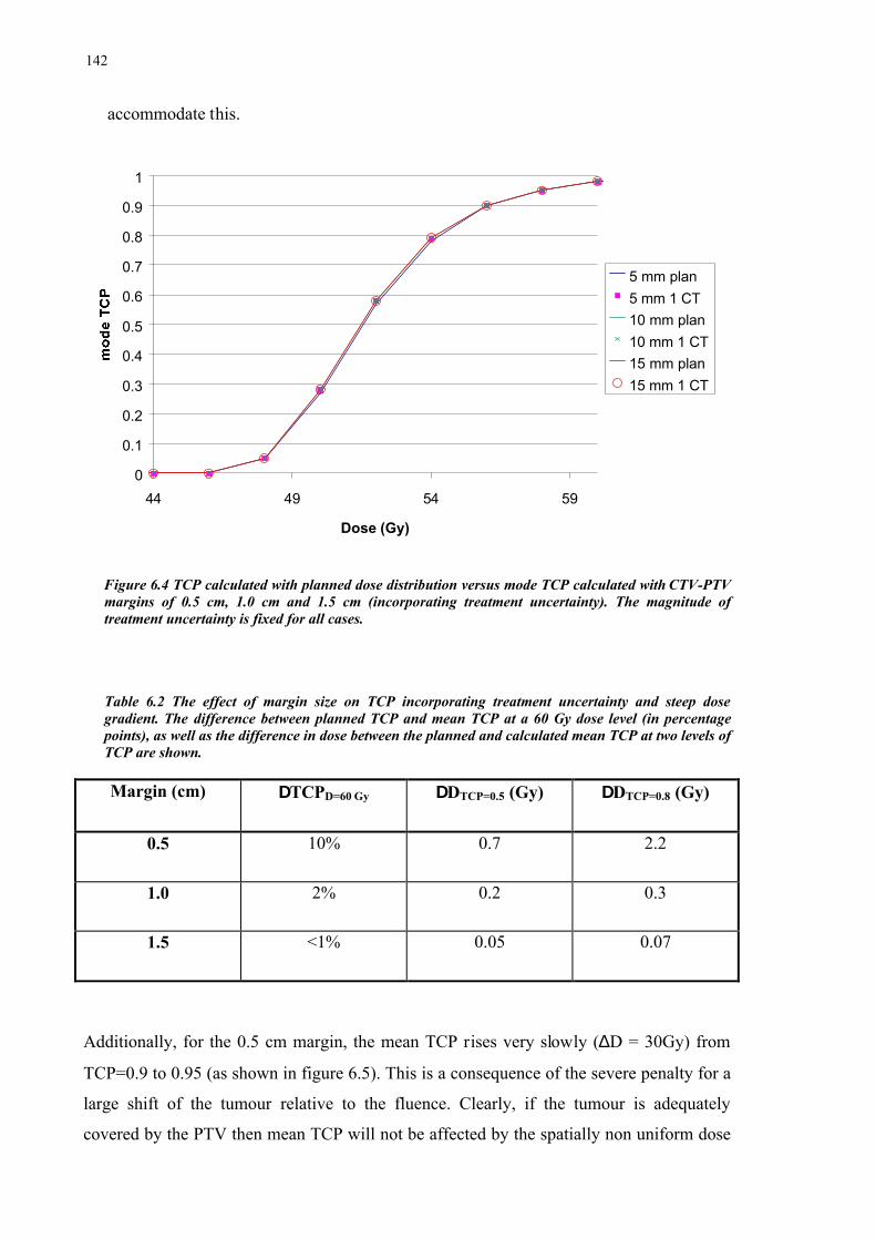
142
accommodate this.
0
0.1
0.2
0.3
0.4
0.5
0.6
0.7
0.8
0.9
1
44 49 54 59
Dose (Gy)
5 mm plan5 mm 1 CT10 mm plan10 mm 1 CT15 mm plan15 mm 1 CT
Figure 6.4 TCP calculated with planned dose distribution versus mode TCP calculated with CTV-PTV margins of 0.5 cm, 1.0 cm and 1.5 cm (incorporating treatment uncertainty). The magnitude of treatment uncertainty is fixed for all cases.
Table 6.2 The effect of margin size on TCP incorporating treatment uncertainty and steep dose gradient. The difference between planned TCP and mean TCP at a 60 Gy dose level (in percentage points), as well as the difference in dose between the planned and calculated mean TCP at two levels of TCP are shown.
Margin (cm) ∆TCPD=60 Gy ∆DTCP=0.5 (Gy) ∆DTCP=0.8 (Gy)
0.5 10% 0.7 2.2
1.0 2% 0.2 0.3
1.5 <1% 0.05 0.07
Additionally, for the 0.5 cm margin, the mean TCP rises very slowly (∆D = 30Gy) from
TCP=0.9 to 0.95 (as shown in figure 6.5). This is a consequence of the severe penalty for a
large shift of the tumour relative to the fluence. Clearly, if the tumour is adequately
covered by the PTV then mean TCP will not be affected by the spatially non uniform dose

143
error. This is supported by the results for the 1.0 cm and 1.5 cm margins that show only
modestly greater values with the smaller penumbra width than the previous results in table
6.1.
The sharper penumbra causes an increase in the standard deviation in mean TCP (see
figure 6.5). Thus, a larger variation in tumour control is evident. The peak values of the
standard deviation in mean TCP are 0.31, 0.15 and 0.06 for the 0.5 cm, 1.0 cm and 1.5 cm
margins respectively. This represents increases of 0.07, 0.05 and 0.02, respectively. The
mean TCP also extends to a higher dose level than with the conventional four field dose
distribution which emphasises the harsh penalty for geographical misses.
0.0
0.1
0.2
0.3
0.4
0.5
0.6
0.7
0.8
0.9
1.0
40 50 60 70 80 90 100
Dose (Gy)
IMRT planmean - 5 mmmean - 10 mmmean - 15 mmSD - 5 mmSD - 10 mmSD - 15 mm
Figure 6.5 Mean TCP calculated using dose distribution with steep penumbra compared with the standard dose distribution.
6.2.3.3. Impact of uniform dose uncertainty and interpatient heterogeneity
Intuitively, the margin size should not affect the variation in TCP due to uniform dose
uncertainty or interpatient heterogeneities because the TCP is calculated with dose to CTV
voxels. Since the margin size (with the exception of margins of less than the distance
between 100% and 95% dose) will not affect the planned CTV dose then it will not affect
TCP incorporating the spatially uniform dose uncertainty or interpatient heterogeneity.
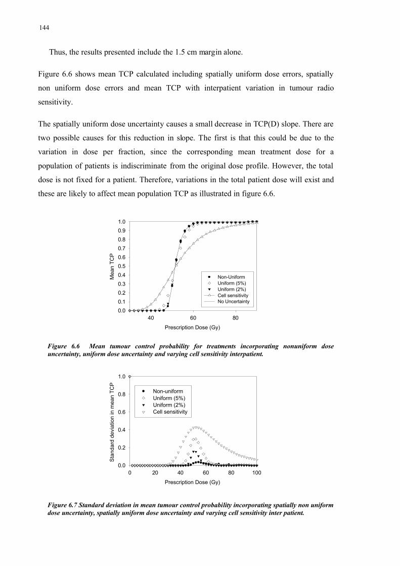
144
Thus, the results presented include the 1.5 cm margin alone.
Figure 6.6 shows mean TCP calculated including spatially uniform dose errors, spatially
non uniform dose errors and mean TCP with interpatient variation in tumour radio
sensitivity.
The spatially uniform dose uncertainty causes a small decrease in TCP(D) slope. There are
two possible causes for this reduction in slope. The first is that this could be due to the
variation in dose per fraction, since the corresponding mean treatment dose for a
population of patients is indiscriminate from the original dose profile. However, the total
dose is not fixed for a patient. Therefore, variations in the total patient dose will exist and
these are likely to affect mean population TCP as illustrated in figure 6.6.
Prescription Dose (Gy)
40 60 80
Mea
n TC
P
0.00.10.20.30.40.50.60.70.80.91.0
Non-Uniform Uniform (5%)Uniform (2%)Cell sensitivityNo Uncertainty
Figure 6.6 Mean tumour control probability for treatments incorporating nonuniform dose uncertainty, uniform dose uncertainty and varying cell sensitivity interpatient.
Prescription Dose (Gy)
0 20 40 60 80 100
Stan
dard
dev
iatio
n in
mea
n TC
P
0.0
0.2
0.4
0.6
0.8
1.0
Non-uniformUniform (5%)Uniform (2%)Cell sensitivity
Figure 6.7 Standard deviation in mean tumour control probability incorporating spatially non uniform dose uncertainty, spatially uniform dose uncertainty and varying cell sensitivity inter patient.

145
The variation (1 standard deviation) in TCP at particular dose levels is shown in figure
6.7 for each of the uncertainties. The magnitude of uncertainty in mean TCP for a given
dose level is dependent on the slope of the TCP(D) curve at that dose level. The magnitude
of the variation (1SD) in mean TCP is shown to be large and can be larger than the mean
value itself. An upper limit of TCP equal to unit is enforced. Bear in mind that the
population TCP distributions are not Gaussian. Therefore straight-forwardly combining the
quoted means and standard deviations will often give non physical results i.e. probability
greater than one or less than zero.
Considering this, the distribution of TCP over a patient population allows clarification of
the potential impact of these three types of uncertainty on the treatment outcome. For the
case of zero uncertainty, the distribution of TCP values will take the form of a delta
function at the single value of TCP corresponding to the prescribed dose and specified
tissue properties. Figure 6.8 shows the distribution of TCP for a patient population, with
TCP calculated to separately include the three types of uncertainty at three prescribed
doses. The three prescribed dose levels were chosen to give a low probability, a midrange
probability and a high probability of tumour cell survival across the patient population. The
TCP calculated without any uncertainties included in the calculation is also shown in
figure 6.8 as a vertical dashed line. The TCP distribution plots are shown with a log
probability scale to illustrate the probability down to very small values. A dashed
horizontal line at TCP = 0.01 highlights and separates the relative number of treatments
with negligibly low probability of tumour control.
Introducing uniform dose uncertainty into the calculation of patient population TCP’s
results in a broadly peaked distribution of patient TCP values, particularly at high and low
doses. At each prescribed dose the uniform dose uncertainty contributes to almost the
complete range of possible tumour outcomes i.e. from no control to complete control. A
significant proportion of the sample TCP values (i.e. those larger than ~0.2) for the 48 Gy
(lowest) prescribed dose have a chance of less than 0.01 of occurring. For the mid-range
prescribed dose (52 Gy), the sample TCP values are evenly distributed with probability of
~0.01. While at the 56 Gy (highest) prescribed dose, those sample TCP values less than
~0.7 have a very small chance of resulting from this dose and the distribution peaks near
the expected sample TCP value. Therefore the mean TCP curve for uniform dose
uncertainty shows a balance between outcomes for different patients. It does not mean that
all patients are likely to have this value of TCP. In fact the number of patients with this

146
TCP could be negligible (see, for example, the curve with variable radio sensitivity in
figure 6.8b).
Sample TCP0.0 0.1 0.2 0.3 0.4 0.5 0.6 0.7 0.8 0.9 1.0
Prob
abilit
y
0.001
0.01
0.1
1
Non-uniform Uniform (5%)Uniform (2%)Cell sensitivity
Dose = 48 Gy
Sample TCP0.0 0.1 0.2 0.3 0.4 0.5 0.6 0.7 0.8 0.9 1.0
Prob
abilit
y
0.001
0.01
0.1
1
Non-uniformUniform (5%)Uniform (2%)Cell sensitivity
Dose = 52 Gy
Sample TCP0.0 0.1 0.2 0.3 0.4 0.5 0.6 0.7 0.8 0.9 1.0
Prob
abilit
y
0.001
0.01
0.1
1
Non-uniformUniform (5%)Uniform (2%)Cell sensitivity
Dose = 56 Gy
Figure 6.8 Distributions of TCP for three dose levels a) 48 Gy, b) 52 Gy, and c) 56 Gy incorporating dose uncertainty (uniform or non uniform) and interpatient cell sensitivity variation. The exact calculated TCP at these dose levels (shown as vertical dashed line) are 0.05, 0.58 and 0.90, respectively.
a)
b)
c)

147
Non uniform dose uncertainty, as mentioned previously, results in relatively small dose
variation within the tumour volume – but this is directly dependent on the margin size and
the magnitude of the treatment uncertainties. Therefore, with the 1.5 cm margin, the non-
uniform dose uncertainty causes sharply peaked distributions of TCP for each dose level,
although it still spreads out slightly from the initial delta functions representing planned
TCP. This is illustrated by the range of sample TCP values with probability greater than
0.001 for each of the dose levels being ~0.05, 0.1, and 0.05 respectively. The most
probable TCP value (the peak) has a probability of very near to one.
Introducing interpatient variation in cell sensitivity results in a wide distribution of tumour
control across the patient population for each prescription dose. All three tested
prescription dose levels give rise to the possibility of complete tumour control and no
tumour control. Moreover, the probability of a patient having a mid range value of TCP is
low. The distribution of sample TCP is peaked at both zero and near one. The most
probable outcome then seems to switch between only these two outcomes with the relative
proportion of each dependant on the dose.
Examining this point further; by neglecting cases with TCP less than 0.01 (below dashed
line) the TCP distributions become bi stable for all three dose levels. This indicates that at
these dose levels the treatment outcome depends primarily on individual patient
radiobiological response (and secondarily on the delivered dose). If the dose is increased
the importance of variation in patient radio sensitivity is reduced because those radio-
resistant tumours are given the dose they require to be eradicated. This point is further
expanded on in the discussion.
Again, population statistics allow further generalisation to the most probable patient
outcome, when each of the uncertainties is separately considered. The mode of TCP versus
dose, shown in figure 6.9, illustrates steep transitions from low probability of tumour
control to a high probability of tumour control across the population. To gauge the
steepness, the curve containing no uncertainty (from figure 6.6)is also featured in the mode
TCP plot. The interval between points on the curve is fixed at the fraction size of 2 Gy.

148
This may limit the steepness of the curves.
Prescription Dose (Gy)
45 50 55 60 65
Mod
e TC
P
0.00.10.20.30.40.50.60.70.80.91.0
Non-uniformUniform (5%)Uniform (2%)Cell sensitivityNo uncertainty
Figure 6.9 Mode of TCP over a patient population.
The uniform dose uncertainty and varying cell sensitivity both give rise to a mode TCP
gradient that is steeper than the mean TCP curve and shifted to higher dose. This suggests
that despite the introduced uncertainties, patient tumour control is highly dependent on
selecting the correct prescription dose. For non uniform dose uncertainty the mean and
mode TCP both closely follow the TCP values calculated without any uncertainty.
The differences between mean and mode TCP occur with relatively large spatially uniform
dose error (5%) and the radio sensitivity. In both of these cases the mode TCP is shifted to
higher dose. This means that a higher dose is required in these circumstances for most of
the population. The mode TCP curves are also steeper than the mean TCP curve for these
two cases. This implies that the threshold dose exists to achieve local control in most of the
population. This threshold dose will be increased with increased treatment uncertainty.
Supporting this, the mode TCP with interpatient cell sensitivity heterogeneity is positioned
at a higher dose than that calculated incorporating uniform dose uncertainty.
Where no treatment uncertainty is present, mode TCP is equal to mean TCP for a
population, and this TCP value will also correspond to the probability of tumour control
for every patient (as they are identical – no uncertainty). Mean values of the dose and radio
sensitivity should, of course, be the same in these two situations.
For a selected range of doses above the threshold dose, most patients, in populations with
variable radio sensitivity or encountering spatially uniform dose errors, will have a higher
probability of local control than those individuals in non variable populations. This reflects
the dose when the mode TCP is greater than the mean TCP for the population, and is

149
evident in figure 6.8 above. The meaning of this can be explicitly demonstrated for the
situation shown in figure 6.8. Consider the prescription dose equal to 54 Gy. In this case
approximately 95% of the patients from the population with variable radio sensitivity
would have a TCP ≈ 1.0 and approximately 5% would have nearly zero TCP. If all patients
would have the same value of radio sensitivity then all of them would have had TCP ≈ 0.8.
6.2.3.4. Results using 3D input data
Three dimensional input data was used to obtain the best estimate of the effect of treatment
errors on tumour control. Generally the radio sensitivity of patients will not be known.
Consequently, interpatient variability in radio sensitivity is modelled as standard across the
patient population.
The impact of systematic errors on the TCP of an individual patient was calculated with
parameters modelling two scenarios; an empty (smaller than average) rectum at planning,
and a full (larger than average) rectum at planning. Obviously, these systematic errors will
impact on the position of the prostate at planning. The mean TCP and standard deviation in
mean TCP (error bars) are illustrated below in figure 6.10.
In the case of an empty rectum in the planning CT scan, the prostate is determined to be
posterior from the mean position. Thus, the prostate will tend to be relatively anterior
during treatment. Conversely, with a full rectum at planning, the prostate will tend to be
relatively posterior during treatment.
0
0.1
0.2
0.3
0.4
0.5
0.6
0.7
0.8
0.9
1
50 55 60 65 70 75
Treatment dose (Gy)
15 mm (F)15 mm (E)10 mm (F)10 mm (E)5 mm (F)5 mm (E)

150
Figure 6.10 TCP calculated for an individual patient with (F)ull or (E)mpty rectum in planning CT scan with margins of 0.5 cm, 1.0 cm, or1.5 cm.
Importantly, the systematic errors are equal in magnitude (in the anterior and posterior
directions) and the margin is uniform. Therefore both systematic shifts should have the
same effect on TCP. This is supported in figure 6.10 by the mean TCP being almost
equivalent for each of the systematic errors.
The error bars associated with each curve in figure 6.10 indicate the potential impact of
random treatment uncertainty. The error bars increase as the margin size is decreased as a
consequence of the increased risk of a geometrical miss.
Across a large population of patients, a range of systematic prostate position errors will
occur. The mean TCP across a population and the standard deviation in mean TCP are
listed in table 6.3 below for three cases including planned (which incorporates the planned,
or intended, dose distribution), random only (which assumes that there is no systematic
error), and systematic and random. All cases include inter patient variation in tumour radio
sensitivity.
Table 6.3 Mean TCP at 64 Gy across a patient population for three margin sizes, with error given as one standard deviation in mean TCP.
Margin Planned Random only Systematic + Random
1.5 0.61 ± 0.32 0.63 ± 0.31 0.60 ± 0.31
1.0 0.62 ± 0.33 0.59 ± 0.32 0.56 ± 0.33
0.5 0.57 ± 0.33 0.53 ± 0.31 0.54 ± 0.33
Three main trends (evident from table 6.3) exist across a population of patients. These
include; negligible change at each margin with or without error, a small reduction in TCP
as the margin is reduced, and an intrinsic uncertainty (SD>0) exists for planned TCP due to
inter patient radio sensitivity variations.
The most prominent effect across the population is the standard deviation in the planned
TCP. Following the plot of standard deviation in TCP from figure 6.7 the maximum value
occurs where TCP is 50%. For the population-based results, the 50% TCP occurs between

151
58 Gy and 63 Gy depending on the margin size. Thus, the values of standard deviation
shown in table 6.3 (at 64 Gy) should be close to their maximum. If the dose level were
increased, this uncertainty could be reduced.
6.2.4. Discussion
In this study, a set value of random positioning error was used. Dose based margin
equations can be used to size the margin (as outlined in §2.7.1.1). Using equation 2.6 with
the values of systematic and random error applied in this study the calculated margins are
14 mm, 16 mm, and 8 mm in the AP, SI and LR direction, respectively. In this study
uniform margins were used. The mean TCP for an individual patient was shown to have a
significant uncertainty associated with a margin of 5 mm. However, the next largest
margin (10 mm) did not demonstrate any deleterious effects from the systematic or random
errors. Clearly, the dose based margin equation does not correlate with the calculated
tumour control. The dose based margin equation naturally does not account for any
radiobiological effects, but it should be emphasised that these equations do not infer any
profound clinical impact, only coverage probability.
The random and systematic errors will evoke larger uncertainty in the TCP with sharply
defined dose distributions. That is, the difference for TCP between an adequate and an
inadequate margin increases. This was indicated by an increase in the standard deviation in
mean TCP for the single field dose profile against the four field conventional dose profile.
The effect of a spatially uniform dose uncertainty on mean TCP was modelled as a 2% or
5% error in the fraction dose. Across a population of patients this error will even out. But
each individual patient will receive a fluctuating fraction dose and a total dose higher or
lower than prescribed. The patient TCP is calculated from the total dose of that patient and
the distribution of sample TCP (refer to figure 6.8) shows a range of outcomes at each
prescription dose. The range extends beyond the planned TCP. This suggests that some
patients with insufficient prescribed dose have a chance at actually benefiting i.e. receiving
higher doses that lead to higher cure rates. For uniform dose uncertainty this results from
the entire irradiated volume receiving higher dose. While for the non uniform dose
uncertainty the maximum tumour dose does not change but the volume of tumour
receiving 100% dose may increase. Certainly, the contiguous normal tissue (such as rectum
or bladder for prostate treatments) would also receive an increased dose in this
circumstance.

152
The variation in cell sensitivity across a population of patients is shown to result in a
double peaked distribution of TCP values across the patient population. This distribution
peaks at TCP values of zero and one, and the probability of mid range TCP values is low
(<1%). The mean TCP for a patient population is shown to be the fraction of patient
population with high (approaching to unit) value of TCP. This results from the
combination of a large relative uncertainty in cell sensitivity and the steepness of the
individual TCP curve with cell sensitivity.
The TCP equation (equation 3.17) can be considered as a function of cell sensitivity for a
fixed dose. Figure 6.11 shows the range of TCP values covered by one and two standard
deviations of cell sensitivity at different dose levels from 48 Gy to 85 Gy. Also shown in
figure 6.11 are the two values for tumour radio sensitivity, α1 and α2, which were used in
the 1D and 3D investigations, respectively.
With the more radio resistant value of cell sensitivity (α 2=0.35 Gy-1) used in the 1D study,
the range of interpatient variation at the lower doses (48 Gy and 56 Gy) covers the range of
tumour outcomes. Furthermore, at the lowest prescription dose, two standard deviations of
variation only permits TCP values barely greater than zero.
0
0.1
0.2
0.3
0.4
0.5
0.6
0.7
0.8
0.9
1
0.1 0.15 0.2 0.25 0.3 0.35 0.4 0.45 0.5
Cell sensitivity (Gy -1)
48 Gy56 Gy75 Gy85 Gy
2 SD
1 SD
α1 α2
Figure 6.11 Plot of TCP versus cell sensitivity. Two values of cell sensitivity (α1 = 0.29 Gy-1, α2 = 0.35 Gy-1) and the range covered by one and two standard deviations in cell sensitivity are illustrated. See text for further description.

153
Some radiotherapy centres (such as Memorial Sloan Kettering cancer centre in the
United States) are escalating dose above 80 Gy. Increasing the dose allows the more radio
resistant tumours that may not have been treated successfully at lower doses to be
controlled. In figure 6.11, the curve for 81 Gy lies in the region well outside 1 standard
deviation from α2, which shows that this dose would control over 68% of the patient
population. On the other hand, this curve is just outside the region covered by 2 standard
deviations. This indicates that 81 Gy would control a little less than 95% of the patient
population. This data is in agreement with the results from MSKCC where they reported
controlling 95% of the population with 81 Gy target dose (Zelefsky 2001). The most recent
value of prostate carcinoma cell sensitivity in the literature, α1 (Sanchez-Neito et al 2001b)
is lower than the value used in the 1D study, α2. This signifies that prostate tumours are
more radio resistant than previously thought. Therefore, with the lower doses shown in
figure 6.11, even for those patients at the higher end of the range of cell sensitivities the
TCP is low. With the escalated doses the TCP the values of TCP are 70% and 98% for the
75 Gy and 85 Gy doses, respectively.
Examining the four dose levels in figure 6.11 at the 50% TCP level the separation between
the two lower dose curves is larger than the separation between the two escalated dose
curves. This highlights the diminishing return (in terms of TCP) as the dose is escalated.
Zagars et al (1987) suggest that the intratumour variation in cell sensitivity is smaller than
the interpatient cell sensitivity. This would reduce the relative uncertainty in cell sensitivity
if we could measure tumour sensitivities for individual patients and not a population. The
magnitude of intratumour variation is still unknown.
Sanchez-Neito et al (2001b) suggest that a small percentage (<1%) of the population are
poorly suited to radiotherapy (due to intrinsic radio resistance) and other treatment options
should be pursued for these patients. Certainly, the distributions of TCP over a population
represented in figure 6.8 agree with this assertion.
In this study, the dose distribution is homogeneous in the PTV with no hotspots or cold
spots. This dose distribution is typical for treating prostate cancer. For other sites, where
hot spots and cold spots exist, spatially non uniform dose errors will have a larger effect.
Sanchez-Neito and Nahum (1999) use the delta-TCP (∆TCP) concept to examine the effect
of hot and cold spots, compared to an original planned dose distribution. The ∆TCP is
calculated as:
154
( ) ( ) ( )( )∑
−⋅⋅=∆
i jij
Pijiij DBCP
DBCPTCPgTCP ,,1 α
αασ α (6.5)
where the differential DVH is used to extract the bin control probability for the jth bin
receiving a dose Dj, and g is the probability of the tumour having cell sensitivity αi.
Sanchez-Neito and Nahum (1999) calculate that the cold spots reduce the TCP by more
than the respective increase from a hot spot of equivalent magnitude. This had been
previously shown with an earlier model for surviving fraction by Brahme (1984).
Therefore the TCP for a patient treated with a heterogeneous dose distribution
incorporating geometric uncertainty would be expected to be reduced from the planned
TCP and the reduction should be indicated by the lowest dose.
6.3. Normal Tissue Complication Probability
Normal tissue complication probability is the probability that a certain percentage of the
patient population will incur unfavourable reactions to the tissue at a particular dose.
6.3.1. Background: Incorporating treatment uncertainty into NTCP
calculation
Fenwick et al (2001) conjectures that the uncertainty in the actual dose deposited from the
planned dose distribution is a factor of some concern. However, prior work of his (Fenwick
1999) had calculated that the impact of setup errors and rectum movements on NTCP is
“surprisingly limited”. Lu et al 1995 investigated the effect of setup errors and rectum
motion on the prediction of NTCP using both DSHs and DVHs. They modelled the effect
of the positioning uncertainty by applying a range of margin sizes and demonstrated that
DSHs provide a more accurate description of NTCP than DVHs. Raggazzi et al 1997
convolved a position PDF with a prostate dose distribution and calculated the resultant
NTCP, with a range of margins and PDF standard deviations. They found that NTCP was
not strongly affected by the errors. But importantly, their method did not account for
fluctuations in dose per fraction, they only accounted for a mean dose. Lebesque et al 1995
serially CT scanned a series of patients through treatment delivery to investigate whether
the DVH, DWH and NTCP derived from the planning CT scan is indicative of the entire
treatment course. They found that the rectum changes shape dramatically, and randomly,
through the treatment. However, the variation in high dose (>90% target dose) wall volume

155
was relatively small (1SD = 14%). Consequently, the NTCP calculated with rectum
(including contents) was approximately equal to NTCP calculated from the rectal wall
inferring that the planning CT could be used confidently.
6.3.2. Methods
Chapter 5 investigated the dosimetric impact of rectal wall motion and patient positioning,
while the current investigation integrates those data into the calculation of the normal
tissue complication probability to further study the effect of these uncertainties.
Normal tissue complication probability for late rectal bleeding is calculated using the linear
quadratic model for FSU (i.e. assumed to be contained with in a voxel) complication
probability and the Källman s-model to combine the voxel complication probabilities into
an organ complication probability. Surviving fraction was calculated for each simulated
patient following the modelled 30 fraction treatment, including the accumulated dose to the
deforming rectal wall as per the model developed in Chapter 5.
6.3.2.1. Fitting Linear-Quadratic parameters to late rectum complications
The literature (Emami et al 1991, Kallman et al 1992, Hartford et al 1996, Metcalfe et al
1997, Sanchez-Neito et al 2001b) provides measured clinical parameters for late rectum
complications (i.e. severe proctisis, necrosis, stenosis and fistula). These parameters
include D50 = 76 Gy (the whole organ dose leading to 50% complication rate), D5 = 60 Gy,
α/β = 3 Gy, and n=0.24 (related to the relative seriality parameter, s=1/n). Normal tissue
complication probability for uniform irradiation of the entire organ is then calculated
using;
( )[ ] ssLQ DPNTCP
1)(11 −−= , (6.6)
where PLQ(D) is the linear quadratic equation for cell killing,
[ ]dDDLQ eNDP βα −−−= 0exp)( . (6.7)
Setting the initial number of FSU’s (N0) to 106, the value of cell sensitivity was manually
adjusted along with the variance in interpatient cell sensitivity to achieve an NTCP curve
that passes through the D5 and D50 values. The fitted value of cell sensitivity for late
rectum complications is α = 0.151±0.023 Gy-1. The value of β used was calculated for each

156
patient using a fixed α/β ratio of 3 and their (sampled) α value.
6.3.2.2. Modelling individual treatments and patient populations
The literature (Rudat et al 1996, Roeske et al 1995, Melian et al 1997 ) describes the
prostate to move randomly in the AP, LR and SI directions. This motion has been strongly
correlated with rectum distension and weakly correlated with bladder filling for patient
positioned supine (Zelefsky et al 1999, Roeske et al 1995). Bladder volume may be more
important for those patients treated prone (Melian et al 1997). In the AP direction we
assume that the prostate is in contact with the anterior rectum wall and the geometric
centre of the rectum is fixed. Thus, prostate position at any time in the AP direction is
assumed to follow the sampled position of the anterior portion of the rectum wall.
The biological effective dose (refer to equation 3.11) for rectal tissue was continuously
calculated following each accumulated fractional dose for each rectum voxel. The voxel
biological effective dose following the entire 32 fraction treatment is combined across the
rectum ROI voxels and used to calculate a sample NTCP value using equation 3.28. A
population of NTCP values is calculated from Ntx simulated treatments. A number of
model parameters of the model are tested including various margin sizes, various levels of
targeting accuracy and various numbers of CT scans used to average prostate position.
Three uniform CTV-PTV margins were tested (0.5, 1.0, 1.5 cm) with the MC code to
calculate NTCP including the effects of systematic organ motion error, and random errors.
A specific dose distribution was created for each margin, such that the 95% isodose
encompassed the PTV.
6.3.3. Results
6.3.3.1. Individual patients
The effect of two separate systematic errors (c.f. §5.3.6 for description of the systematic
errors) on NTCP for an individual patient was investigated. The NTCP values calculated
with full or empty rectum are plotted in figure 6.13 with each of the three planned dose
distributions.

157
00.10.20.30.40.50.60.70.80.9
1
60 70 80 90 100 110 120
Treatment dose (Gy)
15 mm (F)15 mm (E)10 mm (F)10 mm (E)5 mm (F)5 mm (E)
Figure 6.13 Mean NTCP calculated for individual patients with either full (F) or empty (E) rectums in the planning CT scan and with margins of 0.5 cm, 1.0 cm, or 1.5 cm. Table 6.4 NTCP across a patient population (N=1000) with D=64 Gy
During the course of treatment random changes in the rectum radius and beam/patient
positioning will occur and give rise to variation about the mean values. The variation is
indicated in figure 6.13 by error bars. The error bars indicate one standard deviation in
NTCP accounting for the random uncertainty.
Figure 6.13 shows that patients treated using 5 mm or 10 mm margins have negligible
effect from either systematic errors. The mean NTCP calculated using a 15 mm margin
shows an increased complication for the patient with an empty rectum in the planning CT
scan as compared to the patient with a full rectum in the planning CT scan. With the 15
mm margin, almost half of the empty rectum is planned to be included in the PTV. An
empty rectum will consequently imply that the rectum will receive a higher dose during the
treatment. This raises the mean dose and the volume of rectum receiving target dose during
the course of treatment.
In the clinically important region of dose for this particular plan (<70 Gy) the mean NTCP
curves for each systematic error are relatively close (<0.05 separation) and it is only at
higher doses that for the 15 mm margin the two curves separate. The planned dose
distribution used in this study delivered 64 Gy to the PTV and therefore an assumption is
made at higher doses. The assumption is that by systematically increasing the dose the
distribution of dose is still acceptable. At higher doses, the planned distribution of dose to
the rectum may not have been acceptable, and an alternative distribution designed.
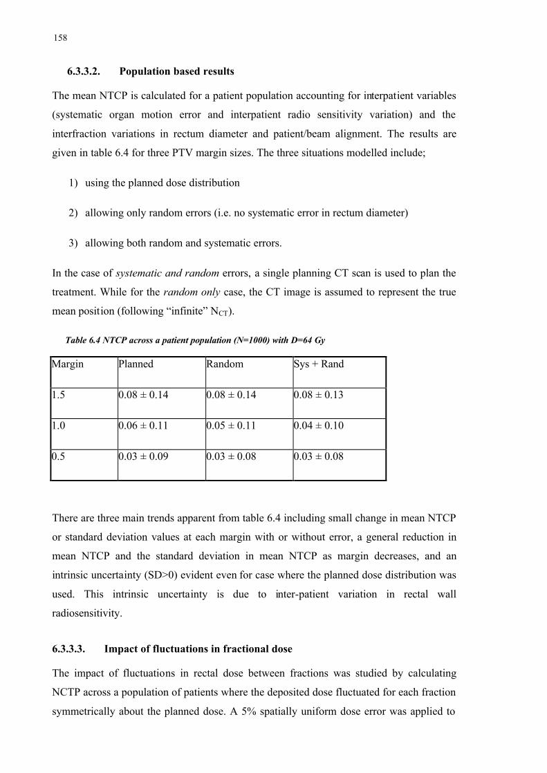
158
6.3.3.2. Population based results
The mean NTCP is calculated for a patient population accounting for interpatient variables
(systematic organ motion error and interpatient radio sensitivity variation) and the
interfraction variations in rectum diameter and patient/beam alignment. The results are
given in table 6.4 for three PTV margin sizes. The three situations modelled include;
1) using the planned dose distribution
2) allowing only random errors (i.e. no systematic error in rectum diameter)
3) allowing both random and systematic errors.
In the case of systematic and random errors, a single planning CT scan is used to plan the
treatment. While for the random only case, the CT image is assumed to represent the true
mean position (following “infinite” NCT).
Table 6.4 NTCP across a patient population (N=1000) with D=64 Gy
Margin Planned Random Sys + Rand
1.5 0.08 ± 0.14 0.08 ± 0.14 0.08 ± 0.13
1.0 0.06 ± 0.11 0.05 ± 0.11 0.04 ± 0.10
0.5 0.03 ± 0.09 0.03 ± 0.08 0.03 ± 0.08
There are three main trends apparent from table 6.4 including small change in mean NTCP
or standard deviation values at each margin with or without error, a general reduction in
mean NTCP and the standard deviation in mean NTCP as margin decreases, and an
intrinsic uncertainty (SD>0) evident even for case where the planned dose distribution was
used. This intrinsic uncertainty is due to inter-patient variation in rectal wall
radiosensitivity.
6.3.3.3. Impact of fluctuations in fractional dose
The impact of fluctuations in rectal dose between fractions was studied by calculating
NCTP across a population of patients where the deposited dose fluctuated for each fraction
symmetrically about the planned dose. A 5% spatially uniform dose error was applied to

159
the calculation of rectal wall NTCP for each of three margin sizes and showed a
minimal change from the NTCP calculated with the planned dose distribution (see figure
6.14).
Mean NTCP calculated with spatially uniform dose error has a reduced gradient from the
planned NTCP and is slightly shifted to lower dose levels. However, both of these effects
are small. In the clinical dose region (< 70 Gy) the mean NTCP is generally increased from
planned NTCP. This indicates that a fluctuating total dose to the normal tissue is more
damaging (on average) across the population than if the planned dose were given. The
increase in mean NTCP at 64 Gy is ~ 0.01 for the 15 mm margin. The increase is less
pronounced as the PTV margin is reduced.
The gradient of the mean NTCP curve including spatially uniform dose error also
decreases as the PTV margin decreases. This indicates a diminishing return (in terms of
NTCP) as the dose level is increased.
0
0.1
0.2
0.3
0.4
0.5
0.6
0.7
0.8
0.9
1
50 60 70 80 90 100 110 120
Dose (Gy)
5mm (5%)10 mm (5%)15 mm (5%)5 mm (plan)10 mm (plan)15 mm (plan)
Figure 6.14 NTCP calculated with planned dose or with a 5% spatially uniform dose error at each fraction of treatment.
Effectively, the trends shown with a spatially uniform dose error infer that the proportion
of patients predicted to suffer complications based on the planned dose, even if the patient
and organs did not move, will be minimally under predicted.

160
6.3.3.4. Comparison with mean treatment dose
As an alternative to calculating NTCP for individual patients and then averaging from the
population of NTCP values, the average dose might be used to calculate NTCP. In this
section, NTCP is calculated in both of these ways and compared.
The mean dose deposited in the rectal wall can be approximated using the precalculated
dose surface map data. Use of the DSM data assumes the thickness of the rectal wall (in
each angular segment of each transverse slice) receives the same dose as deposited at the
outer rectal wall surface. If this assumption is permissible then precalculated (or adaptively
accumulated) dose surface information could feasibly be used to calculate NTCP.
To test this assumption NTCP is calculated with both the planned dose distribution and
also with the DSM from the original dose distribution (see figure 6.15).
Figure 6.15 Comparison between NTCP calculated with the planned dose distribution against NTCP calculated assuming that the planned surface dose (from DSM) is deposited uniformly in each angular rectal wall segment.
For clinical doses figure 6.15 shows that the assumption of uniform dose through the
thickness of each angular segment of rectal wall has a negligible effect on the value of
NTCP calculated. Thus, the precalculated dose surface data can be used to approximate
mean dose in the clinically relevant range of doses. The NTCP calculated using a
precalculated population mean dose is compared in figure 6.16 to the average NTCP across
a population.
00.10.20.30.40.50.60.70.80.9
1
60 80 100 120
Dose (Gy)
10 mm (plan)10 mm (DSM)15 mm (plan)15 mm (DSM)5mm (plan)5 mm (DSM)

161
Figure 6.16 Comparison of mean NTCP calculated with mean dose (mean) against the calculated rectal wall (surface) dose. Both sets were calculated for a population of patients, with each patient being planned from a single CT image set.
In the clinically relevant range of doses (<70 Gy) the NTCP calculated using the mean
dose is close to the NTCP derived from the MC calculation with a 5 mm margin. With a 10
mm or 15 mm margin the value of NTCP calculated with the mean dose is reduced from
the MC calculated. The difference is small (with maximum deviation of 0.02 at 70 Gy) in
this dose range. Neglecting systematic errors, the NTCP calculated using the mean dose is
negligibly different from the MC calculated values in the clinically relevant dose range
(60-80 Gy). The comparison is shown in figure 6.17 for the three margin sizes.
0
0.1
0.2
0.3
0.4
0.5
0.6
0.7
0.8
0.9
1
50 60 70 80 90 100 110 120
Dose (Gy)
5 mm Random only (DSM)
10 mm Random only (DSM)
15 mm Random only (DSM)
5 mm Random only
10 mm Random only
15 mm Random only
Figure 6.17 Comparison of mean NTCP calculated with the mean dose against the MC calculated rectal wall dose. Both sets were calculated for a population of patients, with each patient being planned using the mean organ position.
0
0.1
0.2
0.3
0.4
0.5
0.6
0.7
0.8
0.9
1
50 60 70 80 90 100 110 120
Dose (Gy)
5 mm - surface5 mm - mean15 mm - surface15 mm - mean10 mm - surface10 mm - mean

162
Given that the magnitudes of the deviations in NTCP are quite small the statistical
accuracy of the calculations is paramount. Following that the number of sample treatment
NTCP values averaged was 103 in most cases the standard deviation in the mean values
can be approximated by 310
1 i.e. ~ 3 %. In some cases, a larger number (i.e. 5×10³) of
iterations were done, which increased the precision to ~ 1% for those cases.
6.3.4. Discussion
This work has shown that the impact of geometric errors on the mean NTCP across a
population is small. The simulated treatments included a single magnitude of random
treatment uncertainty across the population. Each simulated patient was modelled with
systematic uncertainty, sampled radio sensitivity and positioning error. Surprisingly, the
NTCP calculated for an individual patient incorporating large systematic errors also had
only a small effect, however the margin size did affect the standard deviation in mean
NTCP.
Other studies have also shown that the effect of organ motion and patient positioning errors
has only a small effect on NTCP (Fenwick 1999, Lu et al 1995, Raggazzi et al 1997).
Theoretically, since the rectum has been shown to produce a volume effect, changes in
percentage volume receiving target dose levels should produce deviations in the calculated
NTCP.
The dose surface maps in Chapter 5 have shown that although large deviations in dose are
possible due to variations in rectum diameter, the geometry of the rectum means that these
changes occur along the lateral rectal walls. Thus, the actual changes in high dose volume
are not large. This is supported by the work of Lu et al (1995) and Lebesque et al (1995).
Lu et al (1995) modelled the effect of organ motion/setup errors by comparing DVHs
against DSHs between margin sizes. They showed that as the proportion of rectum
irradiated increases with margin size the magnitude of the increase is smaller in percentage
surface area than in percentage volume. Lebesque et al (1995) used serial CT scans during
treatment delivery to show that the variation in high dose rectal wall volume was relatively
small (1SD = 15%) and that the change in the high dose volume (<90% target dose) was
proportional to the total volume changes (including filling).
Also contributing to the small effect on NTCP from the treatment uncertainty is the
163
symmetry of the position PDF (Gaussian) used in each case. That is, the probability of
the rectum expanding from the mean position is the same as the probability of contraction.
Thus, interfraction variations will ‘even out’ across an entire treatment. Across a
population of patients the systematic errors, modelled using a Gaussian distribution, will
also average to zero across a large number of patients.
Raggazzi et al (1997) used the Lyman-Kutcher-Burman (LKB) DVH reduction scheme to
calculate NTCP (see also §3.4.2 for description of the scheme). They modelled the effect
of random organ motion errors and patient positioning errors performing a convolution of a
position PDF with a prostate dose distribution and calculating NTCP using the mean dose.
The calculated NTCP values incorporating random errors do produce reductions in NTCP
from the NTCP calculated with the planned dose distribution. They suggest this is due to
the reduction in average dose at the top of the dose distribution penumbra coinciding with
the rectal wall tissue.
Using the model described earlier, NTCP was calculated with two sets of parameters: Set 1
(TD50 = 76 Gy, n=0.12, m=0.15); and Set 2 (TD50 = 76 Gy, n = 0.24, m=0.15). Ragazzi et
al (1997) used values similar to those of Set 1 with TD50 = 80 Gy, however they only
modelled random errors for individual patients. The calculated NTCP values for three
margin sizes and two dose levels (modelled by linearly scaling the DSH) are shown in
figures 6.18 and 6.19 for an individual patient with full (larger than average) rectum at
planning, or empty (smaller than average) rectum at planning. That is, for the individual
we have additionally modelled an empty or full rectum at planning that introduces a
systematic error for that patient.
The NTCP calculated using the mean dose surface histogram with the LKB scheme
predicts higher NTCP than the voxel-based Källman model. Evidently, the parameters and
parameter values are not equivalent between models.
In the figures 6.18 and 6.19 NTCP increases with margin size and is larger for the
treatment delivering 70 Gy to the tumour compared to the 60 Gy treatment. The larger
volume effect is modelled in figure 6.18 (n=0.24). The 60 Gy treatment shows an
increasing variation in NTCP between the two systematic errors as the margin is reduced.
With a larger target dose, the discrepancy between the effects of systematic error is much
reduced, but the overall NTCP is greater. This reflects that 60 Gy is in the middle (of the
NTCP versus dose curve) while 70 Gy is near the upper limit.

164
0.3
0.32
0.34
0.36
0.38
0.4
4 5 6 7 8 9 10 11 12 13 14 15 16
margin (mm)
Empty (60 Gy)Full (60 Gy)Plan (60 Gy)Empty (70 Gy)Full (70 Gy)Plan (70 Gy)
Figure 6.18 NTCP calculated using the mean dose with n=0.24, m=0.15 for an individual patient with systematic error.
0
0.05
0.1
0.15
0.2
0.25
0.3
0.35
0.4
4 5 6 7 8 9 10 11 12 13 14 15 16
margin (mm)
Empty (60 Gy)Full (60 Gy)Plan (60 Gy)Empty (70 Gy)Full (70 Gy)Plan (70 Gy)
Figure 6.19 NTCP calculated using the mean dose with n=0.12, m=0.15 for an individual patient with systematic error.
The serial structure of the rectum (Hall, 2000) should produce a steeper increase in NTCP
with dose once the threshold dose is surpassed. In figure 6.19, the lower dose level (60 Gy)
with the 0.5 cm margin predicts zero NTCP for an empty rectum at planning. As the
165
margin is increased the NTCP appears to increase at an increasing rate, however since
there are only three data points one cannot be sure. Certainly, with n=0.12, the 70 Gy
curves show a larger spread of NTCP values between the situation modelled than with
n=0.24.
The mean dose surface histogram calculated across a population is also used to calculate a
population based estimate of NTCP. Naturally following from the DSHs, the NTCP did not
vary significantly from that calculated using the planned dose distribution.
Importantly, the DSH reduction schemes assume that the mean dose gives the same
amount of complications (i.e. calculated NTCP) as the calculation with fluctuating fraction
dose. It has been shown for NTCP that the fluctuation in fraction dose deposited in rectal
tissue does produce a deviation in the calculated NTCP. The deviation will be dependent
on the margin size.
The models and their parameter values used in this study have been taken from the
literature and are believed to be feasible. However, they are based on incomplete clinical
data, and care should be taken when extracting clinical conclusions from the results.
6.4. Uncomplicated tumour control probability (UTCP)
The uncomplicated tumour control probability provides a single value of the probability of
a favourable outcome. If normal tissue complication is considered equally detrimental as
tumour control is considered beneficial then equation 3.31 can be used. More generally, the
weight of importance placed on a given complication is closer to reality.
6.4.1. Methods
Uncomplicated tumour control probability is calculated using equation 3.31 for a
population of patients with various configurations of error incorporated. The calculation of
UTCP is carried out for each patient of the population. A general assumption is that the
motion of the anterior portion of rectal wall is correlated with the anterior-posterior motion
of the prostate gland.
The individual patient is modelled with a single value of radio sensitivity and systematic
organ motion error. The systematic error will be either a full rectum at planning (which
166
will push the prostate anterior in the planning CT scan) or an empty rectum at planning.
Random errors are simulated through the course of each simulated treatment. The random
errors include deformation of the rectum (modelled as changes of rectum radius and
associated changes of rectal wall thickness), motion of the prostate, patient setup errors
(spatially non uniform dose error) and spatially uniform dose error (SUE, assumed to be
5% of fraction dose).
The interpatient uncertainties include variation in the radio sensitivity of the prostate and
rectum, systematic errors captured in the planning CT scan, as well as all uncertainties
attributed to individual patients (see above). The radio sensitivity of the tumour and rectum
are assumed to be uncorrelated. No literature was found to support or oppose this
assumption. The systematic error includes rectum deformation from the mean treatment
size and the associated shift of the prostate in the planning CT scan. The systematic error
can be reduced by averaging organ location from a number of pre treatment CT scans as
described in earlier sections.
6.4.2. Results
6.4.2.1. UTCP calculated for an individual patient
Calculations of mean UTCP with systematic errors simulated at planning are shown in
figure 6.20 below for the three margins investigated. The error bars indicate one standard
deviation due to the random treatment errors (including prostate and rectal wall motion as
well as patient setup errors).
With a 5 mm margin mean UTCP is calculated to peak with target dose 70 Gy and a UTCP
value of 0.94. Neither of the systematic errors have a notable effect on the value of UTCP
calculated. At doses smaller than the peak UTCP dose, the prostate TCP is dominant. Thus,
in this dose range the variation in UTCP is significant (1SD in mean UTCP ~ 0.1) due to
the insufficiency of the 5 mm margin to cover the prostate on all occasions i.e. a
geographical miss is possible with this margin size.
The mean UTCP calculated with a 10 mm margin with either full or empty rectum at
planning showed negligible effect on the value of mean UTCP for the individual patient.
The peak value of mean UTCP will be at dose 69 Gy with mean UTCP equal to 0.97. The
small influence on UTCP from the systematic errors arises from the margin being large

167
enough to avoid geographical misses and not too large to cause significant increases in
NTCP. The NTCP for rectum is relatively quickly varying with increases in high dose
volume (compared to other normal tissues) (Emami et a. 1991). However, since the dose
variation occurs in the lateral rectal wall, the change in volume is small.
0
0.2
0.4
0.6
0.8
1
50 70 90 110
Treatment dose (Gy)
15 mm (F)15 mm (E)10 mm (E)10 mm (F)5 mm (F)5 mm (E)
Figure 6.20 Mean UTCP calculated for a population of identical patients with fixed systematic error.
With a 15 mm margin the mean UTCP peaks with target dose 68 Gy at a UTCP value of
0.96. For target dose lower than the peak value of UTCP the effect of the systematic errors
are negligible because in this dose range the TCP dominates and the 15 mm margin is more
than sufficient to avoid geographical misses of the prostate. However, for doses larger than
the peak dose, the NTCP dominates the UTCP value. In this range of doses a difference
does exist between the UTCP calculated with full or empty rectum at planning. Those
patients planned with empty rectum at planning have a smaller calculated UTCP than those
patients planned with full rectum at planning. This agrees with the NTCP results for
individuals (refer to figure 6.19) where the curve with empty rectum is above that for the
full rectum since UTCP is proportional to (1-NTCP). The variation in UTCP due to the
random errors is negligible with a 15 mm margin.
6.4.2.2. Population based results
The value of mean UTCP for a population varies from that calculated for an individual
patient because the patients will have varying radio sensitivities and their treatment plans
will include varied magnitudes of systematic error. The peak value of mean UTCP

168
averaged across the patient population, the standard deviation in mean UTCP and the
dose required for this peak value are tabulated in table 6.5 below.
Table 6.5 Maximum value of mean UTCP across a population with 1 SD uncertainty. The dose required for maximum UTCP is given in brackets. The planned situation includes no errors.
Margin (mm) Sys + Rand Random only S.U.E. (5%) Planned
5 0.61±0.28 (74) 0.60±0.29 ( 72) 0.58±0.28 (72) 0.64±0.28 (72)
10 0.61±0.28 (70) 0.59±0.30 (72) 0.56±0.29 (70) 0.61±0.30 (68)
15 0.60±0.30 (67) 0.58±0.30 (68) 0.56±0.30 (68) 0.59±0.29 (68)
Comparison of the figures in table 6.5 with those extracted from figure 6.17 leads to three
primary differences between treating a varied population of patients and an individual
patient. These differences include the population based calculations of mean UTCP being
spread over a larger range of doses than for the individual patients, the mean UTCP is
generally lower for the population and the population shows larger variation in mean
UTCP. These differences are mainly due to variation in radio sensitivity between patients.
The peak value of UTCP is minimally affected by the margin size. This is demonstrated by
the largest increase in peak UTCP (from table 6.5) with margin reduction being 0.05. That
increase in peak UTCP is present with the planned case, while for each of the modelled
errors the increase is reduced to ~0.02. However, the deposited dose giving the peak UTCP
does change with the margin size.
The largest value of mean UTCP is calculated for the case with the smallest margin
combined with the nominal planned dose distribution, and the smallest value of mean
UTCP with the 5% spatially uniform dose error. The highest dose needed for peak UTCP
is calculated with the smallest margin because the penumbra is too close to the prostate.
As with the calculations of TCP and NTCP, the calculation of UTCP demonstrates a large
variation between patients. Table 6.5 shows that across all modelled cases the variation in
mean UTCP ranges from 0.28 to 0.30 for peak UTCP. Considering this size of the standard
deviation of UTCP, the differences between results accounting and not accounting for
systematic errors are small. Also, the variation in mean UTCP is minimally affected by the
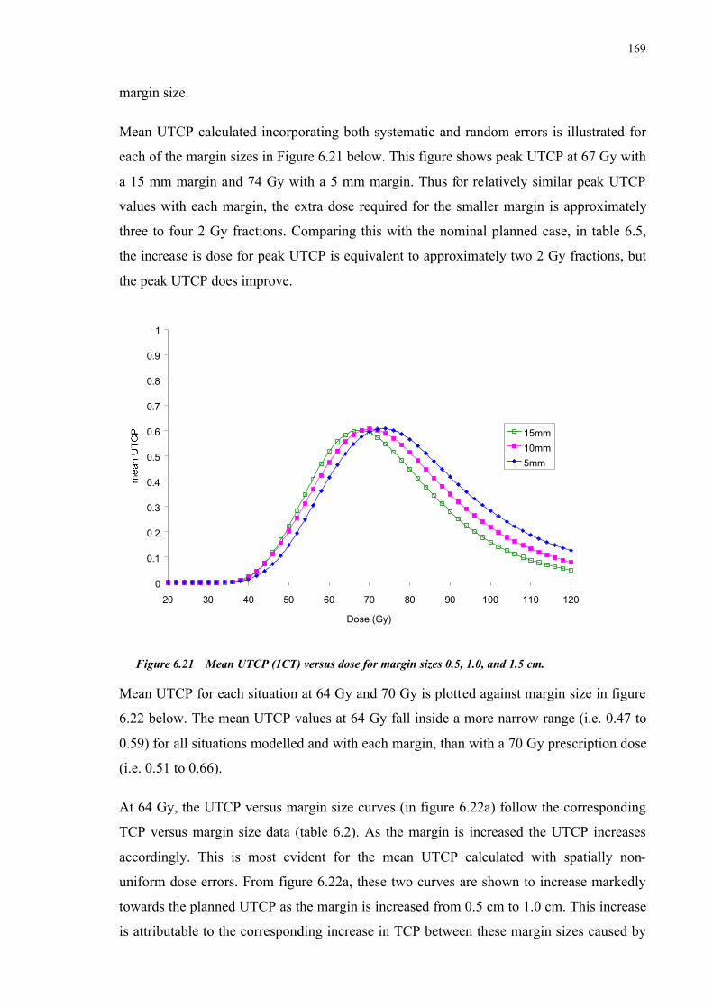
169
margin size.
Mean UTCP calculated incorporating both systematic and random errors is illustrated for
each of the margin sizes in Figure 6.21 below. This figure shows peak UTCP at 67 Gy with
a 15 mm margin and 74 Gy with a 5 mm margin. Thus for relatively similar peak UTCP
values with each margin, the extra dose required for the smaller margin is approximately
three to four 2 Gy fractions. Comparing this with the nominal planned case, in table 6.5,
the increase is dose for peak UTCP is equivalent to approximately two 2 Gy fractions, but
the peak UTCP does improve.
0
0.1
0.2
0.3
0.4
0.5
0.6
0.7
0.8
0.9
1
20 30 40 50 60 70 80 90 100 110 120
Dose (Gy)
15mm10mm5mm
Figure 6.21 Mean UTCP (1CT) versus dose for margin sizes 0.5, 1.0, and 1.5 cm.
Mean UTCP for each situation at 64 Gy and 70 Gy is plotted against margin size in figure
6.22 below. The mean UTCP values at 64 Gy fall inside a more narrow range (i.e. 0.47 to
0.59) for all situations modelled and with each margin, than with a 70 Gy prescription dose
(i.e. 0.51 to 0.66).
At 64 Gy, the UTCP versus margin size curves (in figure 6.22a) follow the corresponding
TCP versus margin size data (table 6.2). As the margin is increased the UTCP increases
accordingly. This is most evident for the mean UTCP calculated with spatially non-
uniform dose errors. From figure 6.22a, these two curves are shown to increase markedly
towards the planned UTCP as the margin is increased from 0.5 cm to 1.0 cm. This increase
is attributable to the corresponding increase in TCP between these margin sizes caused by

170
improved targeting accuracy. The curve for systematic and random errors is located at
lower UTCP than the curve for random errors only. Across a patient population, the
additional systematic error has a detrimental effect on the mean tumour control.
0.45
0.47
0.49
0.51
0.53
0.55
0.57
0.59
0.61
0.4 0.6 0.8 1 1.2 1.4 1.6
Margin size (cm)
plansys+randrand only5%
D = 64 Gy
0.5
0.52
0.54
0.56
0.58
0.6
0.62
0.64
0.66
0.4 0.6 0.8 1 1.2 1.4 1.6
Margin size (cm)
plansys+randrand only5%
D = 70 Gy
Figure 6.22 Mean UTCP against margin size at a) 64 Gy and b) 70 Gy..
At 70 Gy, the UTCP versus margin size curves (in figure 22b) follow the corresponding
TCP versus margin size data (table 6.2) except for the 1.5 cm margin. With a 70 Gy
a)
b)

171
prescription dose and a 1.5 mm margin the NTCP begins to rise as shown in figure 6.19
above. Consequently, the curves for systematic plus random position errors and random
positioning errors appear to become asymptotic in figure 6.22b as the margin is increased.
At both dose levels (64 Gy and 70 Gy) the spatially uniform random dose error with
standard deviation 5% of prescription dose tends to follow the shape of planned UTCP
curve at lower values of UTCP. This is a product of the corresponding TCP values, which
are reduced by the fluctuating dose (as shown in figure 6.5). At these dose levels the NTCP
does not vary from the planned NTCP (as shown in figure 6.14).
6.4.3. Discussion
The calculation of UTCP has included an equal weighting of NTCP and TCP (refer to
equation 3.31). This implies that a complication is of equal detriment to the benefit of
tumour control and therefore the weighting will impact on the conclusions made. Infact,
most of these conclusions may have been made from the separate calculation of TCP and
NTCP. Further clinical value might be obtained from unequal weighting of TCP and NTCP
(such as with equation 3.37), however, the determination of each of the weightings would
add a further estimated variable.
The use of UTCP in this investigation does not seek to endorse equal weighting of the
tumour control and normal tissue reactions. The aim is to provide a simple combination of
benefit against detriment to highlight the importance of margin size, reinforcing the
conclusions of the previous sections. That is, a margin of 5 mm combined with the values
of setup error and organ motion is probably too small, while conversely a margin of 15 mm
is probably too large. Moreover, the UTCP itself is not intended to provide the ideal
margin size, at least due to equal footing of control and complication.
From the planned dose distribution, calculation of UTCP appears to indicate that the ‘best’
margin size (of those tested) is the 1.0 cm margin. However, incorporating treatment
uncertainties into the calculation demonstrates that this may not be the case. The ‘best’
margin may be larger than 1 cm.
The calculation of an optimal margin was shown in §2.6.1 to compensate for systematic
and random positioning errors only. It should also include biological indices such as the
tumour control probability and/or normal tissue control probability. Van Herk et al (2001)

172
presented research linking TCP with functions describing population distributions of
certain treatment uncertainties (c.f. §2.6). Lind et al (1993) optimised a dose profile to
account for geometrical uncertainty. These works lead to the ultimate goal of
radiobiological optimisation, that provides a holistic approach to radiotherapy as outlined,
for example, by Lof et al (1998). Lof et al (1998) seek to optimise the uncomplicated cure
probability (P+) based on four stochastic functionals; fluence, biological, fractionation and
temporal components. Being derived from stochastic variables, P+ itself will be stochastic
and optimisation algorithms calculate the expectation value, EP+.
Patient positioning errors will influence the fluence profile incident to the tumour, and
combined with organ motion, deformation and density changes will influence the temporal
deposition of dose to the tumour. To overcome this temporal component the exact position,
geometry and density of all organs will need to be known on each given treatment day.
Practical concerns come into consideration to gather such information without their
acquisition becoming invasive and the labour input outweighing the therapeutic gain.
However, as a first approximation some general forms of distributions (predominantly
Gaussian) have been used to investigate the optimisation method (Lof et al 1998).
Through the optimisation process, particularly for inverse treatment planning, the
prescription of a margin around the CTV may become redundant. Instead, beam portals are
designed that are functions of all the known treatment parameters. Naturally, the planner
will not know whether the position of organs inside any particular patient will be more or
less variable than the population data for that treatment technique. Therefore, the planner is
required to apply, at least, the population statistics and at most the maximum values
obtained from the population statistics to the generation of an intended dose distribution.
The use of population statistics may not apply to the individual. Hence the initiation of
adaptive radiotherapy, which seeks to initially consider individuals as conforming to the
population distribution of treatment uncertainty while thorough imaging studies are
performed to individualise the treatment to that patients position statistics (and ultimately,
their biological condition). The UTCP could be used in this adaptive process.
From the current work, the status of the rectum in the planning CT image did not cause
significant variation to UTCP for individual patients. However, across a patient population
the inter-patient variation in UTCP was large (with standard deviation typically ~0.3, or
40%). This is predominantly due to the inter-patient variation in rectum radiosensitivity

173
being large (with standard deviation 15% of the mean). At the standard dose levels
investigated (i.e. less than 70 Gy) the dose variations alone did not substantially affect the
mean UTCP. This is gauged from the results for individual patient simulations where
radiosensitivity was fixed. However, with the 0.5 cm margin, the mean UTCP did vary
(with standard deviation ~0.1) at lower doses due to low and variable TCP.
6.5. Conclusions
Uncertainty in the dose deposited to tumour and normal tissue has been shown to impact
on the biological indicators of TCP, NTCP and UTCP. The clinical example of treating
prostate carcinoma with a four field box technique using three different uniform margins
was used to test the sensitivity of a number of treatment uncertainties on calculated
outcome. The outcome (simulated as TCP, NTCP and UTCP) for an individual patient, as
well as averaged across a population of patients was calculated.
The prostate TCP was insensitive to the magnitude of geometrical errors with treatment
margins of 10 mm and 15 mm. However, reducing the margin to 5 mm, produced a
considerable variation in patient TCP across the population. Fluctuations in the dose were
shown to reduce the gradient of mean TCP against dose. The effect on mean TCP from the
dose uncertainties were masked beneath the considerable interpatient variation in radio
sensitivity.
The dose deposited in rectal wall tissue varies noticibly between treatment fractions.
However no significant change in mean NTCP was calculated. This agrees with the
conjecture of Fenwick (2001) and calculations of Raggazzi et al (1997) and Lu et al
(1995). The effect on mean NTCP from the dose uncertainties were masked beneath the
considerable interpatient variation in radio sensitivity. Interestingly, fluctuations in fraction
dose did affect the mean NTCP. Figure 6.14 compared NTCP calculated with the intended
dose distribution against NTCP with variable fraction (using a standard deviation in dose
of 5%). The fluctuating dose causes the gradient of the mean NTCP curve to reduce in
similarity with the effect of fluctuating dose on the TCP. This leads to the mean NTCP
curve crossing the planned NTCP curve. However, the rectum’s volume effect plays a role,
as illustrated in this figure by the mean and planned NTCP curves crossing at higher doses
as the margin was reduced. Considering the geometrical errors, the volume of rectum
receiving high dose fluctuated between fractions (as implied from the variation in rectal

174
surface area from the dose surface histograms in Chapter 5, refer to figure 5.12). NTCP
calculated using the distribution of dose within the width of the rectal wall was shown (see
figure 6.15) to be very close to the NTCP calculated with data from the dose surface
histograms (i.e. uniform dose from each rectal wall surface voxel). This extenuated that the
variations in volume receiving high dose were surprisingly low since they coincided with
narrow lateral walls of the rectum.
In the dose range presented in figure 6.22, incorporating treatment errors leads to mean
UTCP that increases with margin enlargments from 0.5 cm to 1.5 cm and possibly beyond.
In this dose range UTCP follows the relation between TCP and margin size, because the
prescribed dose was not high enough to cause substantial rectal complication probability.
However, the 0.5 cm margin was more heavily penalised for geographical misses of the
tumour. The dose-based estimate of optimal margin size from van Herk et al (2001) is 0.8,
1.4, 1.6 cm in the LR, AP and SI directions respectively. In this study, the outcomes are
predominantly dependent on the AP margin because of the assumed interaction between
anterior-posterior rectal wall movement and prostate motion. Therefore, comparing the
UTCP results with the calculated AP margin, this study shows that the biological
parameters are less sensitive than the dose-based calculations to treatment variations.

175
Chapter 7
Treatment planning algorithm
corrections to account for and display
dose uncertainty in radiotherapy
7.1. Introduction
7.1.1. Possibilities for future radiotherapy treatment planning
From the literature discussion in Chapter 2 it is clear that a number of uncertainties within
the treatment planning process are compromising technological improvements in
radiotherapy. The major treatment uncertainties include patient positioning, organ
motion, and region of interest delineation. The literature review in Chapter 2 also
described a number of modern methods to reduce/account for these uncertainties.
In the holistic approach to RTP the discussion and basis for this chapter may be woven
into each of the techniques discussed in that review. The uncertainty in radiotherapy
needs to be reduced for many reasons, but there are currently limits to the amount by
which it may be reduced. That is, even if the patient is rigidly fixed to the couch each day
of treatment, imaged, and (re-)planned in that position an uncertainty still exists. For

176
example, incorrect tumour delineation because of a lack of biological information in the
CT image or simply poor contrast, machine output fluctuations, radio resistant tumour (or
radio sensitive normal tissue). If daily imaging is too labour intensive (for the entire
treatment) then predictive techniques need to be developed and knowledge from serial
CT studies need to be implemented.
Ten Haken et al (2001) presented a statistical method to include both patient and
population specific distributions of uncertainty. Other workers have presented work with
a similar goal (Lof et al 1998, Mageras et al 1999) fuelled by interpatient differences and
the chance that any given patient may not conform to the population distribution.
7.1.2. Purpose
An uncertainty in the dose delivered to target and normal tissues exists. Moreover, the
fluctuations in delivered dose may have an effect on tumour and normal tissue responses
to radiation. It is therefore important to include in treatment planning systems a means to
evaluate the potential errors and predict their (dosimetric and radiobiological) relevance.
Accordingly, the effect of potential errors could be accounted for more extrinsically in
the planning process.
Furthermore, the current treatment planning algorithms could be improved to (optionally)
include the statistics of random errors and systematic errors. This can be achieved for
each of the 3 most common groups of treatment planning algorithms including
correction-based (Milan/Bentley with inhomogeneity correction) calculations,
convolution/superposition, and Monte Carlo.
Once the basic input data (i.e. beam and uncertainty data) has been included into the
treatment planning computer, visualisation tools are necessary to evaluate their effect. A
number of visualisation tools are explored in this chapter.
In addition to visualisation, these tools would also be used in comparison of rival plans.
Information accrued relating to the treatment errors may be used for predicting suitable
CTV-PTV margins, however, added value may be achieved by also allowing planners to
177
visualise dose related ramifications of certain choices; hence further intellectualising the
decision making.
7.2. Modifications to dose calculation algorithms for photons
Current treatment planning software enables the user to calculate the dose deposited in
tissue based on CT images and linear accelerator output information. The algorithms used
require slightly different input data to calculate dose and have associated accuracies. The
most common dose calculation technique is the correction based technique, but the more
recent convolution/superposition technique* will soon become the most widely available.
Monte Carlo techniques have long shown promise but have not been presented in
commercial systems yet.
With each of these dose calculation techniques, there is a natural point in the dose
calculation process where the inclusion of uncertainty could be placed. In this section, the
algorithms are outlined and that ‘natural’ point where dose uncertainty could be placed
and accounted for is highlighted.
7.1.3. Correction based techniques
7.2.1.1. Input data
The calculation of dose using the correction-based techniques involves a large amount of
input data to characterise the beams from each linear accelerator. This data usually
include a depth dose curve and several profile curves stored for a range of field sizes and
each available beam energy. The data is measured in a water tank in the conditions
specified by the TPS manufacturers.
* referred to as the superposition technique to avoid confusion with the previous convolution techniques
described in earlier sections.
178
A dose distribution for a particular treatment beam and patient configuration is then
determined by manipulating these data. Major consideration is given to factors including
the position and shape of the patient external contour with respect to the beam and
density variations, or inhomogeneities, within the patient.
7.2.1.2. Dose calculation
Dose calculation with correction-based techniques involves correcting the measured dose
data according to the CT density and other information. The basic dose calculation model
was proposed by Milan and Bentley in the early 1970’s (Milan et al 1974). The original
model was improved through the years to correct for changes in SSD, surface curvature,
and basic (effective pathlength) inhomogeneity correction. The dose to a point (x,y) could
then be calculated from
( ) ( ) ( )2
1
max11,,,,
+
+′=
xSSDdSSD
FSydLFSdGyxD seff (7.1)
where G is the infinite SSD dose (measured), L is the off axis ratio, and the third term is
the SSD correction. The infinite SSD dose is calculated for the effective depth, deff, and
field size at the surface, FSs, with the inverse square law removed. The effective depth is
calculated using the densities in the path of the photon beam from the CT density
information as the equivalent depth in water. The off-axis ratio at depth, d, off-axis
distance, y′ (projected to that at the reference SSD) and field size, FS1 (projected to
reference SSD). The last term in equation 7.1 accounts for changes in the SSD from those
in the reference conditions, where x is the current SSD.
The Milan/Bentley model calculates dose reasonably accurately in water equivalent
media, but density heterogeneities have been shown to be poorly predicted. This is
because of the simplistic manner with which the model accounts for heterogeneities, that
is, without including the complexities of scattered photons or secondary electrons.

179
More recent inhomogeniety correction techniques calculate the dose near
inhomogenieties more accurately than the effective pathlength method. Some of these
include, in increasing sophistication, effective depth method, Batho power law method,
equivalent tissue air ratio (ETAR) method, differential scatter air ratio (DSAR) method,
the delta volume method, and fast fourier transform (FFT) convolution method. Most of
the treatment planning systems in the 1990’s used this style of correction based technique
for calculating dose corrected for the clinical situation.
Figure 7.1 Correction factors for various inhomogeneity correction techniques versus depth in different density media. Taken from Wong and Purdy (1990).
As expected, the figure shows that the 3D non scatter ray trace methods (ETAR and FFT)
are clearly superior in accuracy to the 1D non scatter ray trace methods (RTAR and
BATHO). Furthermore, Wong and Purdy (1990) calculated the mean difference between
the calculated and measured doses for each inhomogeneity correction technique. That
comparison showed the 1D techniques to vary about their mean with standard deviation
of 7.72% and 4.14%, for the RTAR and BATHO techniques, respectively. While the
comparison between 3D techniques both showed standard deviations of about 3%. A
number of other, less complex, geometries were also tested with similar results.
180
7.2.1.3. Including estimations of error
The dose data available to manipulate with the correction based dose calculation
techniques is limited to a set of measured dose points. To include error in the calculation,
a new set of source data will have to be calculated from the original measured data. The
calculations are aimed to model the “equal” set of data which would have produced the
same dose distribution in a static patient as realistic data set produces in the patient
subjected to positioning errors and organ motion. Positioning errors and organ motion can
only be accounted for as combined error.
7.1.4. Superposition technique
The superposition technique for calculating dose uses is a model based method. This
means that beam data is collected and used to characterise a model for that beam. Each
calculation of dose will then be based on that model.
7.2.1.4. Input data
Characterisation of a particular treatment beam will typically include measurements of
the depth dose, off axis ratio, and wedge factors for all field sizes. The characterisation
involves generating a model of the incident fluence. This may be done by fitting
parameters in the software such that the prediction agrees with the measured data.
7.2.1.5. Dose calculation
The general form of the superposition dose calculation equation for a polychromatic
beam in an inhomogeneous media, is
( ) [ ] rdr
rrHrrHrrTr
rDave
we
r aveSavePwe ′
′′−+′−⋅′′= ∫ ′
3)(),(),()()(
)(1
ρρ
ρρρρ
. (7.2)
where the term ρ(r) is the density at vectorial point r in the medium, T(r′) is the TERMA
calculated at point r′, rew(r′) is the relative electron density of the media compared to
water at point r′, Hp is the primary kernel, Hs is the scatter kernel.

181
TERMA is the total energy imparted to the medium by the interactions of primary
photons, and the kernels represent the energy imparted about a primary photon interaction
site, as a fraction of the TERMA at that site. The deposition and interaction sites/voxels
are illustrated in figure 7.2. The kernel will equal the sum of primary and scatter kernels.
The kernels for each voxel are usually calculated through a MC process. The TERMA for
the region of interest (where dose calculation is to take place) will usually be calculated
before the actual dose calculation.
Figure 7.2 The superposition dose calculation technique models primary fluence interactions at r′ and the probability of dose deposition in surrounding voxels, including that voxel centred at r. Adapted from Metcalfe et al. (1997).
The literature has shown many examples of complex geometry where the superposition
dose calculations are more accurate than those using correction based methods. Regions
of sharp change in density are, however, not accurately modelled with the superposition
algorithm. Metcalfe et al (1997) show an over estimate of dose in an air cavity and under
estimation after the air cavity. These results are reproduced in figure 7.3.
7.2.1.6. Including estimations of error
The superposition technique calculates a fluence profile prior to dose calculation. This
provides an advantage over the correction based technique, in that the patient positioning
errors are more naturally accounted for in the fluence rather than the dose (Lof et al

182
1998). This is because patient positioning errors will affect the location that each beam is
incident. In this case patient positioning error can be considered separately from organ
motion. This would result in the fluence being convolved with a patient positioning error
distribution function, then the incident fluence itself has been ‘corrected’ for uncertainty
before it is used for dose calculation. Therefore, the effect of uncertainties near
heterogeneities can be more accuratley estimated.
Figure 7.3 The superposition dose calculation overestimates dose in lower density media and underestimates after lower density media. Taken from Metcalfe et al. (1997).
Accounting for organ motion can be done using convolution or MC based techniques.
The convolution technique will be faster than the MC, but has important assumptions that
should be understood, including the number of treatment fractions, and translation motion
only etc.

183
7.1.5. Monte Carlo technique
The Monte Carlo method calculates the deposited dose from first principles and models
the interactions of incident particles along their path length. The most common MC
method used in radiotherapy is EGS4 (Electron Gamma Shower† version 4) and is used
below to exemplify the MC method. Currently, most TPS (treatment planning system)
manufacturing companies are in the process of producing MC based TPS, but there are
not many systems on the market. The knowledge has been available for many years to be
able to do this, but the lack of computing power (and reasonably accurate results with the
superposition technique) has slowed the introduction of this technology.
7.2.1.7. Input data
The EGS4 MC code is a computer program containing three main parts: the user code,
the EGS4 system code and PEGS4 file. Only the third of these is completely an input file.
The PEGS4 file specifies the physical properties of each material in the given geometry.
These include cross sections, mean free paths, and electron stopping powers.
The user code does contain some precalculation parameters, such as incident beam
specifications (fluence, energy spectrum etc), and the output requirements of the
simulation (e.g. dose deposited in voxels). The user code also performs functions during
the process including recording the parameters of interest, recognizing when a transport
step will place a particle in a new region, and outputting results.
The EGS4 system code is generally not accessed by the user and it contains the routines
to actually transport each particle through the medium.
7.2.1.8. Dose calculation
Dose calculation involves following incident particles as they deposit energy in the
medium until they fall below a threshold energy. The incident particle is followed in
† Website: http://www.slac.stanford.edu/egs/

184
steps, that is, after a pre determined distance the status of that particle is reassessed. At
this stage generation of electrons is modelled when the particle under consideration is a
photon. If this is an electron, energy deposition to the media is modelled at each step of
the trajectory. Inter fraction fluence or variations would not be modelled though. The new
status is based on the probability of the particle undergoing certain interactions and will
depend on the particle energy and current medium. When the predetermined lower energy
cut-off is reached the remaining energy is deposited at that step.
A large number of incident particles are required, due to the stochastic nature of the
interactions, to reduce the uncertainty of the result. The uncertainty of the result will also
be dependent on the cut-off energies and step size (distance to next interaction) chosen.
The large number of incident photons will create an even larger number of low energy
electrons in the medium. Generally the uncertainty will only reduce as the square root of
the increased number of incident particles. Therefore, the number of particles must be
quadrupled in order to halve the uncertainty. Much effort has been expended to reduce
the uncertainty in MC results and improve the efficiency (Keall et al 2000). Three of
these techniques are geometric interrogation, Zonal discard, and the repriprocity
technique (Metcalfe et al 1997).
7.2.1.9. Including estimations of error
The inclusion of dose uncertainty into an MC technique, such as EGS4, would be
relatively straight forward (as compared to other the techniques). For MC based dose
calculation techniques the uncertainties can be potentially included in a number of places
including within the user code.
The incident beam fluence may be manipulated to better reflect the interfraction or
interpatient mean fluence distribution. The geometry of the patient can be manipulated to
account for organ motion. This would best be accomplished with detailed data, but again
predictive power is limited to population data in most cases. Still, multiple CT image
studies could be shown on screen with the dose calculated to accommodate patient
positioning errors.

185
7.3. Requirements for display input data
The visualisation technique will obviously depend on the data available to be displayed.
In this section the possible variables that are available to be plotted are discussed.
The most common variables for plotting would be the mean dose and the standard
deviation in dose. Such parameters can be extended to calculation of modified DVH’s
(e.g. CL-DVH), BED calculations with mean treatment dose or variable dose per fraction,
and other biological indices including equivalent uniform dose, TCP, or NTCP.
A number of methods have been proposed to calculate the standard deviation in mean
fraction dose across a treatment, and mean treatment dose across a patient population.
Methods to calculate the standard deviation in dose are briefly outlined below, together
with discussion of non-standard deviations in dose. Non standard deviations, perhaps a
colloquial term, refers to the characterisation of dose PDFs that are not Gaussian and was
used by Goitein (1983).
7.1.6. Standard deviations
For a particular patient the standard deviation in dose can be calculated from (Zavgorodni
1997,Lujan et al 1999):
( ) ( ) ( )( ) ( )zzyyxxgzyxDzdydxdzyxDzyxD −′−′−′×−′′′′′′= ∫∫∫ ,,,,,,,, 220σ (7.3)
where D02 is the planned dose to a point x′, y′, z′; g is the spatial PDF describing random
setup uncertainties, and D is the mean dose. The mean dose can be calculated using
techniques described in chapter 4 (i.e. MC or convolution).
For a population of patients, the systematic error for each patient will be distributed about
the mean systematic error of the population. In chapter 4 the MC method was used to

186
calculate the standard deviation in dose across a patient population, including systematic
uncertainty.
7.1.7. Non standard deviations
In chapter 4 (refer to §4.2) the distribution of dose errors was shown to be Gaussian only
in those (very small sections) of dose distribution where the dose changes linearly
distance. In all other sections of the dose distribution, the dose PDF will be non-Gaussian.
Consequently, the mean will not coincide with the mode, and the standard deviation may
not give a clear indication of the spread of dose values (see figure 7.4 below). In this
case, the mode and FWHM (Full Width at Half Maximum) may be more useful, but these
parameters will be position dependent.
The cause of this non-Gaussian dose PDF is of course the physical limits of maximum
and minimum dose. This was discussed in §4.2.2. At doses near the maximum dose, say
at 99% of the maximum dose the probability of reducing this dose due to misalignment is
the same as an increase, however, the increase is limited to 100%. A larger range of lower
dose values exists and the dose PDF will be non-Gaussian.
For the case of non-standard deviations, one way to express them would be to assign a
mean value. With estimated standard deviation (Goitein 1983) this would then look like,
for example, 99% (+0.5% / -2%). The estimated standard deviation could be calculated
from the dose PDF as the definite integral from the mean or mode to the point on the
curve where the integral equals 0.66/2 (i.e. 1 SD) of the total integral.
Some of the techniques to display the parameters mentioned above are outlined and
illustrated in the next section.
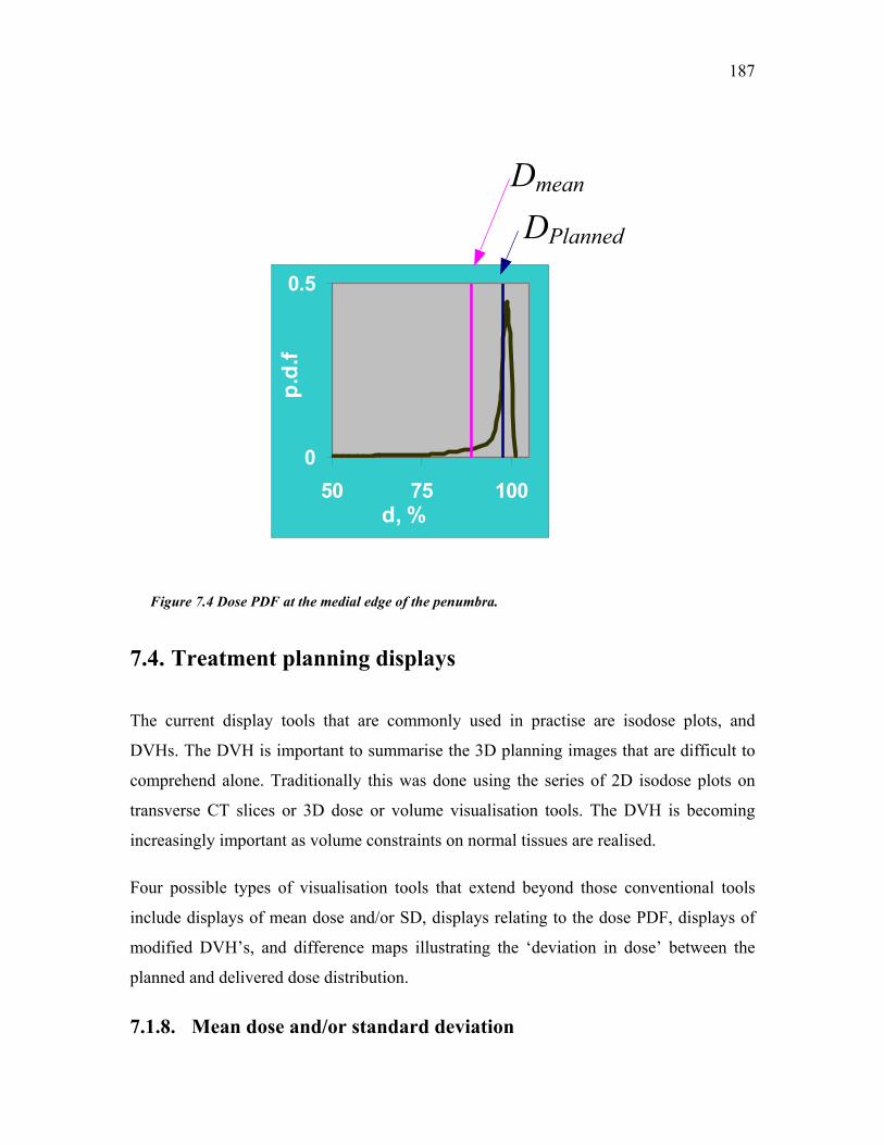
187
0
0.5
50 75 100d, %
p.d.
f
DPlanned
Dmean
Figure 7.4 Dose PDF at the medial edge of the penumbra.
7.4. Treatment planning displays
The current display tools that are commonly used in practise are isodose plots, and
DVHs. The DVH is important to summarise the 3D planning images that are difficult to
comprehend alone. Traditionally this was done using the series of 2D isodose plots on
transverse CT slices or 3D dose or volume visualisation tools. The DVH is becoming
increasingly important as volume constraints on normal tissues are realised.
Four possible types of visualisation tools that extend beyond those conventional tools
include displays of mean dose and/or SD, displays relating to the dose PDF, displays of
modified DVH’s, and difference maps illustrating the ‘deviation in dose’ between the
planned and delivered dose distribution.
7.1.8. Mean dose and/or standard deviation
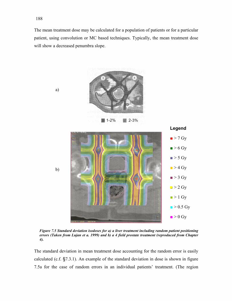
188
The mean treatment dose may be calculated for a population of patients or for a particular
patient, using convolution or MC based techniques. Typically, the mean treatment dose
will show a decreased penumbra slope.
Figure 7errors (T4).
The standa
calculated
7.5a for th
a)
b).5 Standard deviation isodoses for a) a liver treatment including random aken from Lujan et a. 1999) and b) a 4 field prostate treatment (reprod
rd deviation in mean treatment dose accounting for the rando
(c.f. §7.3.1). An example of the standard deviation in dose is
e case of random errors in an individual patients’ treatme
Legend
■ > 7 Gy
■ > 6 Gy
■ > 5 Gy
■ > 4 Gy
■ > 3 Gy
■■■ > 2 Gy
■ > 1 Gy
■ > 0.5 Gy
■ > 0 Gy
patient positioning uced from Chapter
m error is easily
shown in figure
nt. (The region

189
illustrating 2-3% dose uncertainty is outlined in black.) This visualisation tool would
enable the user to clearly understand where the uncertainty in dose occurs and the
expected range of delivered doses. The interpatient standard deviation in treatment dose
can also be displayed in the same way, as isocontours or as a colour wash (figure 7.5b).
a)
b)
Figure 7.6 a) Mean isodose contours, and b) Confidence limit plot showingreceived by 90% of the population.
Legend
■ 100.0%
■ 99.5%
■ 99.0%
■ 98.0%
■ 95.0%
■■■ 90.0%
■ 80.0%
■ 70.0%
■ 50.0%
the minimum dose

190
Confidence limit plots featuring, for example, the mean plus or minus a number of
standard deviations in dose may also be useful. Figure 7.6 shows a confidence limit plot
of mean dose minus 2 standard deviations, which demonstrates the minimum dose
received by 90% of the population. The planner would be able to notice that in figure
7.6b the 90% isodose line (purple) indicating the minimum value sampled from 90% of
the population is inside the left prostate border.
For a more biologically relevant expression of the effect of dose uncertainty, the
biological effective dose could be displayed. Although, displays of BED will have
discontinuities at tissue interfaces this reflects tissue/tumour response more explicitly
because the BED calculation depends on the tissue properties of the irradiated organ.
7.1.9. Modified dose volume histogram
The DVH is a convenient method to summarise the 3D information from a particular
treatment plan. Many authors have used the DVH to highlight the different doses
deposited to a volume of interest after each days treatment measured with serial CT
studies (Lattanzi et al 1999, Zelefsky et al 1999).
Through the prediction of volume of interest dose Mageras et al (1999) have proposed
the confidence limited (CL) DVH (c.f. §2.5). Briefly, the CL-DVH describes a mean
dose DVH, according to specified confidence limits (see figure 7.8a). Naturally, the
confidence limits will depend on the number of fractions delivered. Lujan et al (1999)
showed the reduction in uncertainty about the mean as the number of fractions increased
using a DVH (see figure 7.8b).
7.1.10. Mean with estimated standard deviation display
To calculate a standard deviation assumes that the dose at that point is normally
distributed about the mean. Clearly, from the dose PDFs discussed previously, this is not
the case. At positions medial to the penumbra the deposited dose will more likely
decrease than increase, and vice versa at points lateral to the penumbra. In this case, the
non symmetric estimated standard deviations will need to be displayed.

191
c)
a)
b)
Figure 7.8 The CL-DVH from Mageras et al (1999) a) for prostate and b) rectum, and b) the DVH accuracy increases with the number of fractions (from Lujan et al 1999)
Given the dose PDF of each voxel, a range of parameters can be plotted similarly to the
conventional isodose plots. These are the mean dose and modal dose. In analogy with the
standard deviation, the FWHM can be calculated and also the distance from the mean
value including 95% of responses. This (latter) distance will highlight the tendency of the
probability because dose uncertainty in the upper region of the planned penumbra will
more likely show decreases in dose than increases and vice versa. Ofcourse, depicting the
uncertainty is difficult and displaying more than one isodose with error bars would be
confusing for the viewer. Therefore, each isodose should be viewed separately with it’s
error bars as shown in figure 7.9 below. The MC derived G(D) functions (refer to §4.2.2)
may therefore be used to calculate the +% and -% for particular situations.

192
mode a) b)
+1 ESD
mode -1 ESD
Figure 7.9 Schematic of the a) 95% modal isodose, and b) 30% modal isodose with error bars indicating a 95% chance of depositing given dose.
7.1.11. Difference maps
The difference between planned and delivered dose can be illustrated with difference
maps (Lujan et al 1999). Lujan et al (1999) calculated difference maps for liver dose
including the effect of random patient positioning errors, as shown in figure 7.9.
Figure 7.10 Single axial slice showing lateral and AP beam orientation, b) dose difference display:

193
0DD − . Taken from Lujan et al. (1999).
Difference maps have been used for many years in allied fields as a simple way to view
gross changes in images or matrices.
7.5. Critical evaluation of uncertainty display tools
There are many factors affecting the success of tools in treatment planning software
including; ease of use, value, scientific integrity and marketing of the tool. If a tool was
available to display the uncertainty in dose, it is understandable, that for some planners
the visualisation of ‘error’ or ‘uncertainty’ in dose could be unsettling. For other planners,
this visualisation tool could be reassuring. In this chapter a number of tools have been
introduced or discussed and in this section they will critically evaluated for usefulness,
ease of implementation and value. The scientific integrity of each tool has already been
discussed, and the marketing of any such tool is not relevant to this thesis. The author
believes that true value will only be achieved from dose uncertainty display tools if they
are used together with current display tools, such as isodose plots, surface maps (of 3D
structures and rectal surfaces), dose-volume or -surface histograms etc.
General concerns for each of the dose uncertainty display tools is organising the data to
be displayed in such a way as not to crowd the viewing screen. For example, when
displaying estimated standard deviations, it would be best to display only one isodose
line/surface with the two estimated standard deviations accompanying it on the screen.
Otherwise, the planner could easily get confused between the multitude of lines, and their
associated meanings.
Another general facility would be to switch between different displays and plans. Thus,
the planner could view the difference between the dose fluctuations in the rectal wall with
the 6 field technique against the fluctuations with the 4 field technique. The question then
is; which plan is better? The answer is to use other tools and make a balanced, educated
decision.

194
Tool 1 mean and/or standard deviation (SD). This tool is relatively simple to implement,
using the convolution technique, if the user has access to some dose display components
of the treatment planning software (Keall et al 1999). As outlined previously, it would be
best to use the incident fluence to acknowledge the influence of tissue inhomogeniety on
mean dose calculation. The author’s intent would be for the planner to be able to switch
between mean and SD displays from the current isodose display.
The value of displaying the mean dose is the realisation that the portion of tissue in the
upper beam penumbra actually receives less than the planned dose, and vice versa in the
lower penumbra. For a particular technique, the mean dose may not differ substantially
between patients; however, it would still be useful to confirm the planners’ experience. In
particular cases, tissue heterogeneities could produce large discrepancies from the
standard plan.
The value of displaying the standard deviation in mean dose is the realisation of both the
magnitude of inter-fraction dose differences, and the location of these differences with
respect to the tumour, organs at risk, and beam penumbra. For a particular technique, the
standard deviation in dose will depend on the gradient of the beam penumbra, number of
beams, method of beam delivery, tissue heterogeneities, and the amount of patient/organ
position variability. The standard deviation in dose may not be as accurate as the
estimated standard deviation, which acknowledges the beam penumbra and care should
be taken to understand the meaning of the display.
Tool 2 - modified dose volume histogram. The importance of defining the statistical
confidence of dose delivery and the volume of tissue receiving each dose level is
paramount for both delivering a high quality treatment and building an accurate database
on biological effect. The user should understand how the data used to create the display
are themselves calculated.
The ideal use of modified dose volume histograms is combined with biological tools
(such as TCP and NTCP) to endorse decision making between rival plans. Biological
tools are currently used to differentiate overlapping DVH’s. For example, Plan 1 has a
higher mean dose for the spinal cord, but Plan 2 has a higher maximum dose for the

195
spinal cord. The structure of the spinal cord and it’s impact on dose response is assessed
through, for example, the seriality variable in the Kallman s-model for NTCP.
Tool 3 estimated standard deviation (ESD). The ESD is potentially a very useful tool to
display the effect of patient/organ position uncertainty on the beam penumbra. The ESD
is also instructive for the planner to develop a thorough understanding of the spatially
non-uniform dose uncertainty by visualising the uncertainty about a number of isodose
levels.
Tool 4 Difference maps. The difference between the planned dose calculated for a
number of plans could be useful to quickly identify the location of benefits of one plan
over another. The difference between a planned dose distribution and a calculation of the
actual dose delivered would be more of an educational tool. Similarly, with the difference
between the calculated actual dose distributions from a plan with 1 planning CT image
and another plan with 5 planning CT images.
Most of the above considerations have regarded forward planning and in some ways the
above discussion has moved away from the recommendations of the ICRU. That is, there
is little discussion regarding the internal margin or the setup margin, only the clinical
target volume. The IM and SM seem to be inflexible measures that feed the incorrect
notion that dose uncertainty is not stochastic, or at least the solution cannot be stochastic.
The bulk of this thesis has been devoted to deconstructing this notion and, in this chapter,
to provide examples on how to provide visualisation on the variability in dose. The
clinical impact of such display tools would be farther reaching than simply displaying
dose uncertainty, it would educate planners, clinicians and physicists. The simple
implementation of a mean dose display or an ESD display would demonstrate repeatedly
that the planned dose distribution is not what is delivered to the patient. Of course, to
optimise the planned dose should improve the actual delivered dose, but it may not be
optimal. These display tools allow the planner to investigate the impact of certain
stochastic variables themselves.
In the current climate of continuing technological impact on radiotherapy, it is interesting
to suggest ‘ideal’ uncertainty display tools. The ideal uncertainty display tools should

196
contain elements of both dose uncertainty and biological uncertainty. Naturally, to cloud
current estimates of biological effect with the associated uncertainty in parameter values
(with standard deviations around 20% of the mean value) or the models themselves may
unsettle some workers. The ideal tools for displaying dose uncertainty, in the author’s
mind, is a combination of the confidence limited DVH, assessed along side plots of ESD
and maps of isoeffect accounting for biological uncertainty.
7.6. Conclusions
Treatment planning might be positively impacted by the availability of visualisation tools
for assessing potential ‘dose of the day’ and likely variations of the dose. The impact of
visualisation tool will obviously depend on the quantity and quality of uncertainty data.
Each of the three broad types of dose calculation engine has the possibility of using
uncertainty data. Four techniques for displaying uncertainty in deposited dose have been
outlined. Each of these techniques will offer specialised information that can be used to
increase knowledge of potential ramifications of each treatment design.

197
Chapter 8
Conclusions and further research
Uncertainty exists in every step of the radiotherapy process. The systematic and random
components combine to impact on the actual dose delivered to tumour and normal tissue.
The aims of this research, as outlined in Chapter 1, were as follows;
ο
ο
ο
to estimate the difference between the planned and deposited doses in the
prostate gland and rectal wall
to calculate the biological effect of the differences between the planned and
deposited dose
to investigate tools to visualise the uncertainty in dose delivery.
To achieve the first aim the radiotherapy process was modelled using two models: a Monte
Carlo (MC) computer simulation and a novel adaptation of the convolution technique. Both
methods accounted for the major sources of systematic and random treatment uncertainty. The
major sources of treatment uncertainty include systematic and random organ (prostate and
rectum) motion, systematic and random patient positioning errors, and interfraction linear
accelerator output variation. The impact of these uncertainties on delivered dose for an

198
individual patient and also for a population of patients was investigated. The relative
importance of these uncertainties with a number of margin sizes was investigated.
To achieve the second aim the radiobiological response of the prostate gland and rectum were
modelled using radiobiological models from the literature. The impact on local control of the
prostate from the treatment uncertainties was investigated using the linear quadratic model for
cell survival. To investigate the impact of treatment uncertainty on rectal complications, the
Källman s-model was applied. Interpatient variability in radio sensitivity was modelled across
the patient population. The importance of margin size was tested in combination with each of
the uncertainties.
Visualisation tools were investigated to display the uncertainty in delivered dose.
8.1. Major conclusions
The relative importance of the components contributing to uncertainty in the dose delivered to
the prostate gland and rectum wall has been investigated from calculations of biological
indices.
The impact of treatment uncertainties on the delivered dose to the prostate gland and rectum
wall was investigated. The planned dose delivery was with a 4-field box technique and three
margins between the CTV and PTV were used.
Monte Carlo and convolution models were used model the treatment planning and delivery.
Both of the models agreed that random positioning errors will cause a decrease in the
penumbra gradient for individual patients over the course of treatment delivery. Considering
only random positioning errors for an individual patient, the dose deposited at the edges of the
PTV will be decreased from the planned dose. More importantly for the individual patient is
systematic positioning error that will shift the entire dose distribution and may lead to
significant tumour under dosage.
Across a population of patients the systematic positioning errors were modelled to follow a
Gaussian distribution. This effectively increases the standard deviation of the error across the

199
population and results in further smearing of the penumbra. The standard deviation (SD) in
mean treatment dose significantly increases due to systematic error. A three - fold increase in
the dose SD is calculated across a patient population by incorporating the systematic error.
Previous studies did not include the systematic error; however, this investigation demonstrates
it’s importance. Both models showed that the estimation of mean organ position in the
treatment preparation stage, through averaging organ position in multiple CT image sets, does
affect the mean treatment dose delivered. The MC model demonstrated the 3 fold decrease in
dose SD that can be achieved by reducing systematic organ motion error across the patient
population. The theory of combining uncorrelated standard errors in the mean (Montgomery,
1999) has been applied to extend the statistics/dose based margin size equations (Antolak and
Rosen 1999, McKenzie et al 2000) to include multiple pre treatment CT scan organ position
averaging.
The radio sensitivity of prostate carcinoma was fitted to the clinical data and varies between
patients with a standard deviation of 28% as indicated from clinical trials in the literature
(Zagars et al 1987). This uncertainty has been shown to dominate over the dose/position
related errors if the margin is sufficient. Moreover, this variation creates a bi stable
distribution of tumour control across the population. This demonstrates that for the treatment
dose of ~60 Gy the majority of the patients will fall into one of the two categories: those
patients who have high probability of tumour control, and those who have very low TCP. Only
a small fraction of patients will have TCPs in the region of 0.1 – 0.9 (figure 6.8). This implies
tumour control is less dependent on dose compared to the radio sensitivity of individuals.
However, the dose escalation allows a substantial increase in substantially the number of
patients with expected high TCP (figure 6.11).
Highly conformal dose distributions characterised by steep penumbra gradients were
demonstrated to reduce tumour TCP rapidly (across a patient population) for inadequate
margins. In particular, with a 5 mm margin the TCP reduction of 7% with the standard dose
distribution increased to a reduction of 10% with the steeper penumbra dose distribution.
Furthermore, the dose increase required to retain a mean TCP of 0.8 with the inclusion of dose
uncertainty increased from 0.7 Gy with the standard dose distribution to 2.2 Gy with the
steeper penumbra dose distribution.

200
The modelled rectal deformation caused large deviations in deposited dose from the planned
dose (up to 25%) due organ motion and patient positioning errors. For an individual patient,
the anterior rectal wall will move in and out of the PTV during the treatment delivery if a 5
mm margin is employed. Because the rectum is inevidently in the treatment field, organ
motion and patient positioning errors would reduce the volume of rectum irradiated to over
75% dose (or treatment dose). This happens predominantly when the patient has a full rectum
during the planning CT scan and consequently during treatment the anterior rectal wall will be
posterior to the position in the planning CT image (as shown in figure 5.10).The largest effect
will be with a 5 mm margin, where the percentage of rectal wall receiving high dose (i.e.
>90% of prescription dose) reduces from 17% to 6%.
Conversely, those individual patients with treatments designed using a CT image set where the
rectum is empty may receive larger areas of rectal wall with high dose during treatment
delivery (refer to figure 5.9). Again the plan with a 5 mm margin is more sensitive to dose
variation than the plans with larger margins. The range of deviation in dose from the plan in
that case is ±15 Gy for a 60 Gy prescription dose. Also, the percentage of high dose volume
does not change significantly as shown in the dose surface histogram (refer to figure 5.8).
However, to compensate, the percentage of rectal surface receiving less than 50% of the
prescription dose reduces from 96% to 75%. This highlights the importance of identifying
systematic errors at the planning stage because they do impact strongly on the rectal dose.
Across a population of patients a Gaussian interpatient systematic error will not largely affect
the mean rectal dose. However, the interpatient variation in rectal dose will be significant. The
standard deviation in rectal wall dose is greater than 6 Gy (i.e. 10% of prescription dose) for
some rectal voxels. By averaging CTV position from multiple pretreatment scans the standard
deviation in rectal wall dose can be reduced to less than 2 Gy (averaging from 5 CT acquired
images). The dose surface maps show that as the margin is increased the uncertainty in dose
shifts from the anterior rectal wall to the lateral walls and affects a smaller percentage of the
total rectal wall surface area.
The inter patient radio sensitivity of rectal wall tissue was fitted to the clinical data (Sanchez-
Neito et al 2001b) and it’s standard deviation shown to be to 15% of the mean value. Despite
the large variation in dose deposited to the rectal wall and the volume of rectal wall receiving

201
high dose (>90% of prescription) the NTCP was predominantly affected by the inter-patient
variation in radio sensitivity. At the prescription dose (64 Gy) the mean NTCP across a
population is calculated as 0.08 ± 0.13. This large standard deviation is primarily due to the
inter patient variation in radio sensitivity. The literature presents other studies (Ragazzi et al
1997, Lu et al 1995, Fenwick et al 2001) that concur with the positioning errors having only a
relatively small affect on NTCP. It is concluded that the major dose related effect on NTCP is
due to the mean rectal dose derived from the margin employed. Due to the volume effect
NTCP calculated with the smaller margin was less sensitive to dose variations than NTCP
calculated with the other margin sizes.
Deciding on the optimal margin size is obscured when considering the TCP and NTCP
separately. The composite index UTCP is calculated combining TCP and NTCP with equal
weighting.
This study has highlighted a large difference between the potential doses delivered to
individual patients and that averaged over a patient population. In the absence of generalised
equations to calculate the margin size for individual patients, visualisation of potential dose
discrepancies would be a valued tool. Some of population statistics regarding patient
positioning error, organ motion, delineation errors and linear accelerator output uncertainty are
recommended to be used in the TPS dose calculation algorithm. Further, statistical methods
that adapt the treatment plan to individual patients should be used to shape the geometry and
intensity of delivered fields.
8.2. Further research
Further work is suggested to consider the issues that are outside the scope of this thesis,
particularly;
ο
ο
dose escalation
highly conformal dose distributions, such as those created using IMRT,
tomotherapy or protons.

202
ο
ο
hypofractionation
adaptive radiotherapy
Based on the results in this thesis, these four situations and their potential effect on delivered
dose, local control and complications have been discussed. However, a comprehensive
modelling study to quantify the benefits or otherwise of each would be useful.
The convolution technique was shown to be a quick and accurate technique to calculate the
mean dose and standard deviation, accounting for random translational errors. The MC
technique calculated the standard deviation in treatment dose including also systematic errors.
This was shown to be a useful quantity to calculate. For application of the convolution
technique to account for patient positioning errors, the treatment planning algorithm should
include user input parameters (such as population based patient positioning error variance and
the number of fractions). These should be used to adjust the outgoing fluence so that the dose
computation is more realistic.
With further refinement of the biological models and their parameters, particularly for rectal
complications more detailed investigations of the effects on NTCP will follow.

203
Appendix A The two most recent published papers derived from this thesis work are included in this Appendix. They include: Booth JT, Zavgorodni SF. Modelling the dosimetric consequences of organ motion at CT imaging on radiotherapy treatment planning. Phys.Med.Biol. 46(5):1369-1377. Booth JT, Zavgorodni SF. The effects of radiotherapy treatment uncertainties on the delivered dose distribution and tumour control probability. Australas. Phys. Eng. Sci. Med. 24(2):71-79.


Jeremy T Booth and Sergei F Zavgorodni (2001) Modelling the dosimetric
consequences of organ motion at CT imaging on radiotherapy treatment planning.
Physics in Medicine and Biology, v. 46 (5), pp. 1369-1377, May 2001
NOTE: This publication is included in the print copy of the thesis
held in the University of Adelaide Library.
It is also available online to authorised users at:
http://dx.doi.org/10.1088/0031-9155/46/5/303

Jeremy T Booth and Sergei F Zavgorodni (2001) The effects of radiotherapy
treatment uncertainties on the delivered dose distribution and tumour control
probability.
Australasian Physical and Engineering Sciences in Medicine, v. 24 (2), pp. 71-78,
June 2001
NOTE: This publication is included in the print copy of the thesis
held in the University of Adelaide Library.
It is also available online to authorised users at:
http://dx.doi.org/10.1007/BF03178349

223
1. References
1. Ågren, A., Brahme, A., Turesson, I. 1990 Optimisation of uncomplicated control for head and neck tumors. Int. J. Radiat. Biol. Phys. 19:1077-1085.
2. Ahmad, N.R., Huq, M.S, Corn, B.W. 1997 Respiration-induced motion of the kidneys in whole abdominal radiotherapy: implications for treatment planning and late toxicity. Radioth.Oncol. 42:87-90.
3. Althof, V.G.M., Hoekstra, C.J.M., Te Loo, H-J. 1996 Variation in prostate position relative to adjacent bony anatomy. Int. J. Radiat. Oncol. Biol. Phys., 34(3):709-715.
4. Antolak, J.A., Rosen, I.I. 1999 Planning target volumes for radiotherapy: How much margin is needed? Int. J. Radiat. Biol. Phys. 44:1165-1170.
5. Antolak, J.A., Rosen, I.I., Childress, C., Zagars, G.K., Pollack, A. 1998 Prostate target volume variations during the course of radiotherapy. Int. J. Radiat. Biol. Phys. 42(3):661-672.
6. Balter, J., Chen, G.T., Pelizzari, C., Krishnasamy, S., Rubin, S., Vijayakumar, S. 1993 Online repositioning during treatment of the prostate: A study of potential limits and gains. Int. J. Radiat. Oncol. Biol. Phys. 27:137-143.
7. Balter, J., Ten Haken, R., Lawrence, T., Lam, K.L., Robertson, J.M. 1996 Uncertainties in CT-based radiation therapy treatment planning associated with patient breathing. Int. J. Radiat. Biol. Phys. 36(1):167-174.
8. Balter, J.M., Sandler, H.M., Lam, K., Bree, R.L., Lichter, A.S., Ten Haken, R.K. 1995 Measurement of prostate movement over the course of routine radiotherapy using implanted markers. Int. J. Radiat. Oncol. Biol. Phys., 31(1):113-118.
9. Barensdon, G.W. 1982 Dose fractionation, dose rate and iso-effect relationships for normal tissue responses. Int. J. Radiat. Biol. Phys. 8:1981-97.
10. Beard, C.J., Bussiere, M.R., Plunkett, M.E., Coleman, C.N., Kijewski, P.K. 1993 Analysis of prostate and seminal vesicle motion. Int. J. Radiat. Oncol. Biol. Phys. 27(Suppl. 1):136.
11. Bel A, van Herk M and Lebesque J V 1996a Target margins for random geometrical treatment uncertainties in conformal radiotherapy Med. Phys. 23(9) 1537-1545
12. Bel, A., Keus, R., Vijlbrief, R.E., Lebesque, J.V. 1995 Set-up deviations in wedged pair irradiation of parotid gland and tonsillar tumours, measured with an electronic portal imaging device. Radiother.Oncol. 37:153-159.
13. Bel, A., Vos, P.H., Rodrigus, T.R., Creutxberg, C.L., Visser, A.G., Stroom, J.C., Lebesque, J.V. 1996b High-precision prostate cancer irradiation by clinical application of

224
an offline patient set-up verification procedure, using portal imaging. Int. J. Radiat. Oncol. Biol. Phys., Vol 35, No 2, pp.321-332.
14. Bentel, G.C., Marks, L.B., Sherouse G.W., Spencer, D.P., Anscher, M.S. 1995 The effectiveness of immobilization during prostate irradiation. Int. J. Radiat. Oncol. Biol. Phys. 31(1):143-148.
15. Bijhold. J,, Lebesque, J.V., Hart, A.A.M., Vijlbrief, R.E. 1992 Maximising set-up accuracy using portal images as applied to a conformal boost technique for prostatic cancer. Radiother. Oncol. 24:261-271.
16. Boersma, L.J., van der Brink, M., Bruce, A.M., Shouman, T., Gras, L., te Velde, A., Lebesque, J.V. 1998 Estimation of the incidence of late bladder and rectum complications after high dose (70-78 Gy) conformal radiotherapy for prostate cancer, using dose volume histograms. Int. J. Radiat. Biol. Phys. 41:83-92.
17. Box, G.P.E. 1984 Quoted in 2nd International conference on dose, time and fractionation in radiation oncology. (American Institute of Physics).
18. Boyer, A.L., Schultheiss, T. 1988 Effects of dosimetric and clinical uncertainty on complication-free local tumor control. Radiother. Oncol. 11:65-71.
19. Brahme, A. 1984 Dosimetric precision requirements in radiation therapy Acta Radiol. Oncol. 23:379-391.
20. Brahme, A. 1988 Optimization of stationary and moving beam radiation therapy techniques. Radiother. Oncol. 12:129-140
21. Brahme, A., Ågren, A.-K. 1987 Optimal dose distribution for eradication of heterogeneous tumors. Acta Oncol. 26(5):377-385
22. Brenner, D.J. 2000 (Editorial) Toward optimal external-beam fractionation for prostate cancer. Int. J. Radiat. Biol. Phys. 48:315-316.
23. Brenner, D.J., Hall, E.J. 1999 Fractionation and protraction for radiotherapy of prostate carcinoma. Int. J. Radiat. Biol. Phys. 43:1095-1101.
24. Burman, C., Kutcher, G.J., Emami, B., Goitein, M. 1991 Fitting of normal tissue tolerance data to an analytic function. Int. J. Radiat. Oncol. Biol. Phys. 21:123-135
25. Casamassima, F. 1994 Studies of the mobility of tumour volume Hadrontherapy in Oncology ed U Almaldi and B Larsson (Amsterdam: Elsevier) pp 428-433.
26. Catton, C., Lebar, L., Warde, P., Hao, Y., Catton, P., Gospodarowicz, M., McLean, M., Milosevic, M. 1997 Improvement in total positioning error for lateral prostatic fields using a soft immobilisation device. Radioth. Oncol. 44(3):265-70.
27. Clark, B.G., Souhami, L., Pla, C., Al-Amro, A.S., Bahary, J.P., Villemure, J.G., Caron, J.L., Olivier, A., Podgorsak, E.B. 1998 The integral biologically effective dose to predict brain stem toxicity of hypofractionated stereotactic radiotherapy Int. J. Radiat. Oncol. Biol. Phys. 40:667-75.
28. Corn B.W., Hanks G.E., Schultheiss T.E., Hunt M.A., Lee W.R., Coia L.R. Conformal treatment of prostate cancer with improved targeting: superior PSA response compared to standard treatment. Int. J. Rad. Oncol. Biol. Phys. 27(1), 137-143, 1995.

225
29. Craig, T., Wong, E., Battista, J., van Dyk, J. 1998 The effect of anatomical uncertainties on 3-D conformal treatment planning. Med.Phys. 25(6):1096-1097.
30. Creutzberg, C.L., Althof, V.G., Huizenga, H., Visser, A.G., Levendag, P.C. 1993 Quality assurance using portal imaging: the accuracy of patient positioning in irradiation of breast cancer. Int. J. Radiat. Oncol. Biol. Phys. 25:529-39.
31. Crook, J.M., Raymond, Y., Salhani, D., Yang, H., Esche, B. 1995 Prostate motion during standard radiotherapy as assessed by fiducial markers. Radioth.Oncol., 37:35-42.
32. Dale, E., Olsen, D.R. 1998 (Letter to Editor) Int. J. Radiat. Oncol. Biol. Phys. 40(4):1010-1
33. Dale, E., Olsen, D.R., Fossa, S.D. 1999 Normal tissue complication probabilities correlated with late effects in rectum after prostate conformal radiotherapy. Int. J. Radiat. Oncol. Biol. Phys. 43(2):385-391
34. Davies, S.C., Hill, A.L., Holmes, R.B., Halliwell, M., Jackson, P.C. 1994 Ultrasound quantitation of respiratory organ motion in the upper abdomen. Brit. J. Radiology, 67:1096-1102.
35. Dawson, L.A., Mah, K., Franssen, E., Morton, G. 1998 Target position variability throughout prostate radiotherapy Int. J. Radiat. Oncol. Biol. Phys. 42(5):1155-116.
36. de Boer, H.C., Heijmen, B.J. 2001 A protocol for the reduction of systematic patient setup errors with minimal portal imaging workload Int. J. Radiat. Oncol. Biol. Phys. 50(5):1350-65.
37. Deasy, J.O., Cornett, M.S. 1997 Potential benefit of non-uniform dose distributions delivered using intensity modulation. Med. Phys. 24(6):1021.
38. Ebert, M.A. 2000 Viability of the TCP and EUD concepts as reliable dose indicators. Phys.Med.Biol. 45(2):441-457.
39. Ebert, M.A., and Hoban, P.W. 1996 Some characteristics of tumour control probability for heterogeneous tumours. Phys.Med.Biol. 41:2125-2133.
40. El-Gayed, A.A.H., Bel, A., Vijlbrief, R., Bartelink, H., Lebesque, J.V. 1993 Time trend of patient set-up deviations during pelvic irradiation using electronic portal imaging. Radiotherapy and Oncology, 26, pp162-171.
41. Emami, B., Lyman J., Brown, A., Coia, L., Goitein, M., Munzenrider, J.E., Shank, B., Solin, L.J., Wesson, M. 1991 Tolerance of normal tissue to therapeutic irradiation Int. J. Radiat. Oncol. Biol. Phys. 21:109-22.
42. Epstein B.E. et al. 1992 Low complication rate with conformal radiotherapy for cancer of the prostate. Radiother. Oncol. Suppl. 24:S100.
43. Fenwick, J. D. 2001a. An ntcp formula for the series model with a Yaes-type functional subunit mechanism. Phys. Med. Biol. 46:N33-N38.

226
44. Fenwick, J.D. 1999 Biological modelling of pelvic radiotherapy: Potential gains from conformal techniques (Ph.D. thesis) London University, Internet report ICR/CCO/2000/1; [email protected].
45. Fenwick, J.D. 2001b Impact of dose uncertainties on rectal ntcp modelling II: Uncertainty implications. Med.Phys. 28(4):570-581
46. Fenwick, J.D., Khoo, V.S., Nahum, A.E., Sanchez-Nieto, B., Dearnaley, D.P. 2001 Correlations between dose-surface histograms and the incidence of long-term rectal bleeding following conformal or conventional radiotherapy treatment of prostate cancer. Int.J.Radiat.Oncol.Biol.Phys. 49(2):473-480
47. Fenwick, J.D., Nahum, A.E. 2001 Impact of dose uncertainties on rectal ntcp modelling I: Uncertainty estimates. Med.Phys. 28(4):560-569
48. Fontenla E, Pelizzari C A and Chen G T Y 1996 Implications of 3-dimensional target shape and motion in aperture design Med. Phys. 23(8) 1431-1441
49. Fontenla, E., Pelizarri, C., Roeske, J.C., Chen, G.T.Y. 1997 Non-parametric modelling of organ motion. Med. Phys. 24(6):971.
50. Forman, J.D., Kumar, R., Haas, G., Montie, J., Porter, A.T., Mesina, C.F. 1995 Neoadjuvant hormonal downsizing of localised carcinoma of the prostate: effects on the volume of normal tissue irradiation. Cancer Investigation 13(1):8-15.
51. Forman, J.D., Mesina, C.F., He, T., Devi, S.B., Ben-Josef, E., Pelizarri, C., Vijayakumar, Chen, G.T. 1993 Evaluation of changes in the location and shape of the prostate and rectum during a seven week course of conformal radiotherapy. Int. J. Radiat. Oncol. Biol. Phys. 27(Suppl. 1):222.
52. Fowler, J.F. 1989 The linear quadratic formula and progress in fractionated radiotherapy Br. J. Radiol. 62:679-694
53. Fowler, J.F. 1993 Time-variable dose rate in HDR stepping source brachytherapy. Radiother. Oncol. 29(3):355-6.
54. Fowler, J.F., Chappell, R., Ritter, M. 2001 Is α/β for prostate tumors really low? Int. J. Radiat. Oncol. Biol. Phys. 50(4):1021-31.
55. Frohlich, H., Dohring, W. 1985 A simple device for breath-level monitoring during CT. Radiology, 156:235.
56. Gademann, G. 1996 Definition of target volumes and critical organs Proc. Symp. Principles and Practise of 3-D Radiation Treatment Planning (Munich, 1996) (Munich: Klinikum rechts der Isar, Technische Universitat).
57. Gildersleve, J., Dearnaley, D.P., Evans, P.M., Swindall, W. 1995 Reproducibility of patient positioning during routine radiotherapy, as assessed by an integrated megavoltage imaging system. Radiothe.Oncol. 35:151-160.
58. Goitein, M. 1983 Nonstandard deviations. Med Phys. 10(5):709-11.
59. Goitein, M. 1985 Calculation of the uncertainty in the dose delivered during radiation therapy. Med Phys. 12(5):608-12.

227
60. Greer, P.B., Jose, C.C., Matthews, J.H.L. 1998a Set-up variation of patients treated with radiotherapy to the prostate measured with an electronic portal imaging device. Australasian Radiology, 42:207-212.
61. Greer, P.B., Mortensen, T.M., Jose, C.C. 1998b Comparison of two methods for anterior posterior isocentre localisation in pelvic radiotherapy using electronic portal imaging. Int. J. Radiat. Oncol. Biol. Phys., 41:1193-1199.
62. Hall E.J. 2000 Radiobiology for the radiologist. 5th Ed. Lippincott Williams and Wilkins.
63. Hanley, J., Lumley, M.A., Mageras, G.S., Sun, J., Zelefsky, M.J., Leibel, S.A., Fuks, Z., Kutcher. G.J. 1997 Measurement of patient positioning errors in three-dimensional conformal radiotherapy of the prostate. Int. J. Radiation Oncology. Biol. Phys. 37(26):435-444.
64. Hanley, J., Mageras, G.S., Sun, J., Kutcher, G.J. 1995 The effects of out-of-plane rotations on two-dimensional portal image registration in conformal radiotherapy of the prostate. Int. J. Radiat. Oncol. Biol. Phys. 33(5):1331-1343.
65. Harauz, G., Bronskill, J. 1979 Comparison of the livers respiratory motion in the supine and upright positions: Concise communication. J. Nuc. Med 20:733-735.
66. Hartford, A.C., Niemierko, A., Adams, J.A., Urie, M.M., Shipley, W.U. 1996 Conformal irradiation of the prostate: Estimating long-term rectal bleeding risk using dose-volume histograms Int. J. Radiat. Oncol. Biol. Phys. 36(3):721-730.
67. Haustermans, K. and Fowler, J.F. 2001 Is there a future for cell kinetic measurements using IdUrd or BdUrd? Int J Radiat Oncol Biol Phys. 49(2):505-11.
68. Hoogeman, M.S., de Bois, J.A., Muller-Timmermans, P., van Herk, M., Koper, P.C.M., Boersma L.J., Lebesque, J.V. 2001 The use of 2D-dose maps to determine the effect of organ motion on the dose to the rectal wall. Radiother. Oncol. 61(Supp 1):S37.
69. Howard, A., Cowie, F.G. 1978 Induced resistance in Closterium: Indirect evidence for induction of repair enzyme Radiat Res 75:607-616.
70. Huizenga, H., Levendag, P.C., De Porre, P.M.Z.R., Visser, A.G. 1988 Accuracy in radiation field alignment in head and neck cancer: A prospective study. Radiother.Oncol. 11:181-187.
71. Hunt, M.A., Schultheiss, T.E., Desobry, G.E., Hakki, M., Hanks, G.E. 1995 An evaluation of set-up uncertainties for patients treated to pelvic sites. Int. J. Radiat. Oncol. Biol. Phys. 32(1):227-233.
72. ICRU Report 50 1993 Prescribing, recording and reporting Photon Beam Therapy International Commission on Radiation Units and Measurements, Bethesda, Maryland.
73. ICRU Report 62 1999 Prescribing, recording and reporting Photon Beam Therapy (Supplement to ICRU Report 50) International Commission on Radiation Units and Measurements, Bethesda, Maryland.

228
74. Jackson, A., Slwarchuk, M.K., Zelefsky, M.J., Cowen, D.M., Venatraman, E.S., Levegrun, S., Burman, C.M., Kutcher, G.J., Fuks, Z., Liebel, S.A., Ling, C. 2001 late rectal bleeding after conformal radiotherapy of prostate cancer (II): Volume-effects and dose-volume histograms. Int. J. Radiat. Biol. 49(3):685-98.
75. Joiner, M.C., Marples, B., Lambin, P., Short, S.C., Turesson, I. 2001 Low-dose hypersensitivity: Current status and possible mechanisms Int. J. Radiat. Biol. 49(2):379-89.
76. Jones, K.R. 1982 A respiration monitor for use with CT body scanning and other imaging techniques. Brit. J. Radiology, 55:530-533.
77. Jones, L.C., Hoban, P.W. 2000 Treatment plan comparison using equivalent uniform biologically effective dose (EUBED). Phys. Med. Biol. 45:159-170.
78. Kallman, P., Agren, A., Brahme, A. 1992 Tumour and normal tissue responses to fractionated non-uniform dose delivery. Int. J. Radiat. Biol. 62(2):249-262
79. Kaver, G., Lind, B.K., Lof, J., Lianders, A., Brahme, A. 1999 Stochastic optimisation of intensity modulated radiotherapy to account for uncertainties in patient sensitivity. Phys. Med. Biol. 44:2955-2969.
80. Keall P J, Beckham W A, Booth J T, Zavgorodni S F, and Oppelaar M 1999 A method to predict the effect or organ motion and set-up variations on treatment plans Australas. Phys. Eng. Sci. Med. 22:48-52.
81. Keall P.J., Siebers, J.V., Jeraj, R., Mohan, R. 2000 The effect of dose calculation uncertainty on the evaluation of radiotherapy plans. Med.Phys. 27(3) 478-84.
82. Ketting, C.H., Austin-Seymour, M.. Kalet, I., Unger, J., Hummel, S., Jacky J. 1997 Consistency in three-dimensional target volumes across physicians and institutions. Int. J. Rad. Oncol. Biol. Phys. 37(2) 445-453.
83. Killoran, J. H., Kooy, H. M., Gladstone, D. J., Welte, F. J. and Beard, C. J. 1997 A numerical simulation of organ motion and daily setup uncertainties: implications for radiation therapy. Int. J. Radiat. Oncol. Biol. Phys 37(1):213-221.
84. Kivasaara, L., Makela, P., Aarimaa, M. 1982 Pancreatic mobility: An important factor in pancreatic computed tomography. J. Comp. Ass. Tom. 6(4):854-856.
85. Kron, T., Bazley, S., Roff, M., Hamilton, C., and Denham, J. 1998 A Level 3 Dosimetric Intercomparison for Australasia: A pilot Study. Proceedings of Engineering and the Physical Sciences in Medicine, Hobart, pp12.
86. Kubo, H.D., Hill, B.C. 1996 Respiration gated radiotherapy treatment: a technical study. Phys. Med. Biol. 41(1):83-91.
87. Kuhns, L.R., Thornbury, J., Seigel, R. 1979 Variation of position of the kidneys and diaphragm in patients undergoing repeated suspension of respiration. J. Comp. Ass. Tom. 3(5):620-621.
88. Kutcher, G.J., Burman, C. 1989 Calculation of complication probability factors for non-uniform normal tissue irradiations: The effective volume method. Int. J. Radiat. Oncol. Biol. Phys. 16:1623-1630
229
89. Kutcher, G.J., Burman, C., Brewster, L., Goitein, M., Mohan, R. 1991 Histogram reduction method for calculating complication probabilities for three-dimensional treatment planning evaluations. Int. J. Radiat. Oncol. Biol. Phys. 21:137-146.
90. Kutcher, G.J., Mageras, G.S., Leibel, S.A. 1995 Control, correction, and modelling of set-up errors and organ motion. Sem. Rad. Onc. 5(2):134-145.
91. Lambin, P., Malaise, E.P., Joiner, M.C. 1994 The effect of very low radiation doses on the human bladder carcinoma cell line RT112. Radioth. Oncol. 63-72
92. Langen, K.M., Jones, D.T. 2001 Organ motion and its management. Int J Radiat Oncol Biol Phys. 50(1):265-78.
93. Lattanzi, J., McNeely, S., Hanlon, A., Das, I., Schultheiss, T.E., Hanks, GE. 1998 Daily CT Localisation for correcting portal errors in the treatment of prostate cancer. Int. J. Radiat. Oncol. Biol. Phys. 41(5):1079-1086.
94. Lattanzi, J., McNeely, S., Pinover, W., Horwitz, E., Das, I., Schultheiss, T.E., Hanks, GE. 1999 A comparison of daily CT lcalisation to a daily ultrasound-based system in prostate cancer. Int. J. Radiat. Biol. Phys. 43(4):719-25.
95. Lawton, C.A., Won, M., Pilpech M.V. et al. 1991 Long-term treatment sequelae following external beam irradiation for adenocarcinoma of the prostate: Analysis of RTOG studies 7506 and 7706 Int. J. Radiat. Biol. Phys. 21:935-9.
96. Lebesque, J.V., Bruce, A.M., Kroes, A.P.G., Touw. A., Shouman, T., van Herk, M. 1995 Variation in volumes, dose histograms, and estimated normal tissue complication probabilities of rectum and bladder during conformal radiotherapy of prostate cancer. Int. J. Radiat. Oncol. Biol. Phys. 33:1109-1119.
97. Lee, S.P., Leu, M.Y., Smathers, J.B., McBride, W.H., Parker, R.G., Withers, H.R. 1995 Biologically effective dose distribution based on the linear quadratic model and its clinical relevance Int. J. Radiat. Biol. Phys. 33:375-89.
98. Leong J 1987 Implementation of random positioning error in computerised radiation treatment planning systems as a result of fractionation Phys. Med. Biol. 32(3) 327-334
99. Li, S., Boyer, A., Lu, Y., Chen, G.T.Y. 1997 Analysis of the dose-surface histogram and dose-wall histogram for the rectum and bladder. Med. Phys. 24(7):1107-16.
100. Liebel, S.A., Kutcher, G.J., Zelefsky, M.J., Fuks, Z. 1994 Coping with prostate and seminal vessicle motion in three-dimensional conformal radiation therapy. Int. J. Radiat. Biol. Phys. 28:327-328.
101. Lind, B.K., Kallman, P., Sundelin, B., Brahme, A. 1993 Optimal radiation beam profiles considering uncertainties in beam patient alignment. Acta Oncol. 32:331-342.
102. Ling, C.C., Humm, J., Larson, S., Amols, H., Fuks, Z., Leibel, S., Koutcher J.A. 2001 Towards multidimensional radiotherapy (MD-CRT): Biological imaging and biological conformality. Int. J. Radiat. Biol. Phys. 47(3):551-560.

230
103. Lirette, A., Pouliot, J., Aubin, M., Larochelle, M. 1995 The role of electronic portal imaging in tangential breast irradiation: a prospective study. Radioth. Oncol. 37:241-5.
104. Lof, J., Lind, B.K., Brahme, A. 1998 An adaptive control algorithm for optimisation of intensity modulated radiotherapy considering uncertainties in beam profiles, patient set-up, and internal organ motion. Phys. Med. Biol. 43:1605-28.
105. Logue, J.P., Sharrock, C.L., Cowan, R.A., Read, G., Marrs, J., Mott, D. 1998 Clinical variability of target volume description in conformal radiotherapy planning. Int. J. Radiat. Biol. Phys. 41(4):929-931.
106. Lu, Y., Li, S., Spelbring, D., Song, P., Vijayakumar, S., Pelizzari, C., Chen, G.T.Y. 1995a Dose-surface histograms as treatment planning tools for prostate conformal therapy. Med. Phys. 22(3):279-84.
107. Lu, Y., Song, P., Li, S., Spelbring, D., Vijaykumar, S., haraf, D.J., Chen, G.T.Y. 1995b A method of analyzing rectal surface area irradiated and rectal complications in prostate conformal radiotherapy. Int. J. Radiat. Biol. Phys. 33(5):1121-5.
108. Lujan A E, Ten Haken R K, Larsen E W, and Balter J M 1999 Quantization of setup uncertainties in 3-D dose calculations Med. Phys. 26(1) 2397-2402
109. Lujan, A.E., Balter, J.M., Larsen, E.W., Ten Haken, R.K. 1997 Incorporating both set-up uncertainties and organ motion in the computation of 3-D dose distributions. Med. Phys. 24(6):1022.
110. Lyman, J.T. 1985 Complication probability as assessed from dose-volume histograms. Rad.Res. 104, S-13-S-19.
111. Mackie, T.R., Scrimger, J.W., Battista, J.J. 1985 A convolution method for calculating dose for 15-MV x rays. Med. Phys. 12(2):188-96..
112. Mageras G S, Fuks Z, Leibel S A, Ling C C, Zelefsky M J, Kooy H M, van Herk M and Kutcher G J 1999 Computerised design of target margins for treatment uncertainties in conformal radiotherapy Int. J. Radiat. Oncol. Biol. Phys 43(2) 437-445
113. Mageras, G.S., Melian, E., Fuks, Z., Leibel, S.M., Mohan, R., Kutcher, G.J. 1994 Incorporation of organ motion uncertainties into 3D prostate treatment plans. Int. J. Radiat. Oncol. Biol. Phys. 30(Suppl. 1):175.
114. Malone, S., Crook, J.M., Kendal, W.S., Szanto, J. 2000 Respiratory induced prostate motion: Quantification and characterisation. Int. J. Radiat. Oncol. Biol. Phys. 48(1):105-9.
115. Martinez AA, Gonzalez JA, Chung AK, Kestin LL, Balasubramaniam M, Diokno, A.C, Ziaja, E.L, Brabbins, D.S., Vicini, F.A. 2000 A comparison of external beam radiation therapy versus radical prostatectomy for patients with low risk prostate carcinoma diagnosed, staged, and treated at a single institution. Cancer.88(2):425-32
116. Martinez AA, Yan D, Lockman D, Brabbins D, Kota K, Sharpe M, Jaffray DA, Vicini F, Wong J. 2001 Improvement in dose escalation using the process of adaptive radiotherapy combined with three-dimensional conformal or intensity-modulated beams for prostate cancer. Int J Radiat Oncol Biol Phys. 50(5):1226-34

231
117. McCarter S D and Beckham W A 2000 Evaluation of the validity of a convolution method for incorporating tumour movement and set-up variations into the radiotherapy treatment planning system Phys. Med. Biol. 45 923-931
118. McKenzie, A.L, van Herk, M., Mijnheer, B. 2000 The width of margins in radiotherapy treatment plans.Phys Med Biol. 45(11):3331-42.
119. McParland, B.C. 1993 Uncertainty analysis of field placement error measurements using digital portal image correlations. Med. Phys. 20(3):679-685.
120. Meertens, H., Bijhold, J., Strackee, J. 1990 A method for the measurement of field placement errors in digital portal images. Phys. Med. Biol. 35(3):299-323.
121. Meijer, G.J., van den Brink, M., Hoogeman, S., Meinders, J., Lebesque, J. 1999 Dose-wall histograms and normalised dose-surface histograms for the rectum: A new method to analyse the dose distribution over the rectum in conformal radiotherapy. Int. J. Radiat. Oncol. Biol. Phys. 45(4):1073-80.
122. Melian, E., Mageras, G.S., Fuks, Z., Leibel, S.A., Niehaus, A., Lorant, H., Zelefsky, M., Baldwin, B., Kutcher, G.J. 1997 Variation in prostate position quantitation and implications for three-dimensional conformal treatment planning. Int. J. Radiat. Oncol. Biol. Phys., 38(1):73-81.
123. Metcalfe, P., Kron, T., Hoban, P. 1997 The Physics of Radiotherapy X-Rays from Linear Accelerators. Medical Physics Publishing.
124. Michalski, J. M., Wong, J. W., Gerber, R. L., Yan, D., Cheng, A., Graham, M. V., Renna, M.A., Sawyer, P. J. and Perez, C. A. 1993 The use of on-line image verification to estimate the variation in radiation therapy dose delivery. Int. J. Radiat. Oncol. Biol. Phys. 27:701-716.
125. Milan, J., Bentley, R.E. 1974 The storage and manipulation of radiation dose data in a small digital computer.Br J Radiol. 1974 Feb;47(554):115-21.
126. Moerland, M.A., van der Bergh, A.C.M., Bhagwandien, R., Janssen, W.M., Baker, C.J.G., Lagendijk, J.J.W., Battermann, J.J. 1994 The influence of respiration induced motion of the kidneys on the accuracy of radiotherapy treatment planning, a magnetic resonance study. Radioth. Oncol. 30:150-154.
127. Mohan, R., Mageras, G.S., Baldwin, B., Brewster, L.J., Kutcher, G.J., Leibel, S., Burman, C., Ling, C., Fuks, Z. 1992 Clinically relevant optimisation of 3-D conformal treatments. Med.Phys. 19(4):933-943.
128. Moisenko, V., Battista, J., van Dyk, J. 2000 Normal tissue complication probabilities: Dependence on choice of biological model and dose-volume histogram reduction scheme. Int. J. Radiat. Oncol. Biol. Phys. 46(4):983-993.
129. Montgomery, D. C. 1999 Applied statistics and probability for engineers 2nd ed. New York : John Wiley Sons.
130. Niemerko, A. 1997 Reporting and analyzing dose distributions: a concept of equivalent uniform dose. Med.Phys. 24:103-110.

232
131. Niemerko, A., Goitein, M. 1991 Calculation of normal tissue complication probability and dose-volume histogram reduction schemes for tissues with a critical element architecture. Radiother Oncol. 20(3):166-76.
132. Niemerko, A., Goitein, M. 1993 Modeling of normal tissue response to radiation: the critical volume model. Int J Radiat Oncol Biol Phys. 25(1):135-45.
133. Ohara, K., Okumura, T., Akisada, M., Inada, T., Mori, T., Yokota, H., Calaguas, M. 1989 Irradiation synchronised with respiration gating. Int. J. Radiat. Oncol. Biol. Phys. 17(4):853-857.
134. Oppelaar, M. 1999 Quantifying intrafraction organ motion to better estimate the field dimensions for abdominal radiotherapy MSc Thesis Queensland University of Technology (QUT) Queensland Australia.
135. Padhani, A.R., Khoo, V.S., Suckling, J., Husband, J.E., Leach, M.O., Dearnaley, D.P. 1999 Evaluating the effect of rectal distension and rectal movement on prostate gland position using cine MRI. Int. J. Radiat. Oncol. Biol. Phys. 44(3):525-33.
136. Pavel, L., Rowbottom, C.G., Hector, C., Partridge, M., Bortfeld, T. 2001 Estimation of the effects of movements on dose distribution for prostate patients. Radioth. Oncol. 61 (supp 1):S36.
137. Pickett, B., Roach, M., Rosnethal, S. Horine, P., Phillips, T. 1993 Defining “ideal margins” for six field conformal irradiation of localised prostate cancer (Abstr.). Int. J. Radiat. Oncol. Biol. Phys. 27(Suppl. 1):223.
138. Pisani, L., Lockman, D., Jaffray, D., Yan, D., Martinez, A., Wong, J. 2000 Setup error in radiotherapy: on-line correction using electronic kilovoltage and megavoltage radiographs. Int. J. Radiat. Oncol. Biol. Phys. 47(3):825-839.
139. Pouliot, J., Lirette, A. 1996 Verification and correction of setup deviations in tangential breast irradiation using EPID: Gain versus workload. Med. Phys. 23:253-60.
140. Pradier, O., Schmidberger, H., Weiss, E., Bouscayrol, H., Daban, A., Hess, C.F. 1999 Accuracy of alignment in breast irradiation: a retrospective analysis of clinical practise. Brit. J. Radiol. 72:685-90.
141. Press, W.H., Flannery, B.P., Teukolsky, S.A., Vetterling, W.T. 1989 Numerical Recipes The art of scientific computing. Cambridge University Press.
142. Rabinowitz, I., Broomberg, J., Goitein, M., McCarthy, K., Leong, J. 1985 Accuracy of radiation Field Alignment in Clinical Practice. Int. J. Radiation Oncology Biol. Phys. 11:1857-1867.
143. Ragazzi, G., Manglil, P., Fiorino, C., Cattaneo, G.M., Bolognesi, A., Reni, M., Calandrino, R. 1997 Variations of tumour control probability and rectum complication probabilities due to random set-up errors during conformal radiation therapy of prostate cancer. Radiat. Oncol. 44:259-63.
144. Rasch, C., Barillot, I., Remeijer, P., Touw, A., van Herk, M., Lebesque, J.V. 1999 Definition of the prostate in CT and MRI: A mutli-observer study. Int. J. Radiat. Oncol. Biol. Phys. 43(1):57-66.

233
145. Richie, C.J., Hsieh, J., Gard, M.F., Godwin, J.D., Kim, Y., Crawford, C.R. 1994 Predictive respiratory gating: A new method to reduce motion artefacts on CT scans. Radiology 190:847-852.
146. Roach, M 3rd., Faillace-Akazawwa, P., Malfatti, C. 1997 Prostate volumes and organ movement defined by serial computerised tomographic scans during three-dimensional conformal therapy. Radiation Oncology Investigations 5(4):184-94.
147. Roeske, J.C., Forman, J.D., Mesina, C.F., He, T., Pelizzari, C.A., Fontenla, E., Vijayakumar, S., Chen, G.T. 1995 Evaluation of changes in the size and location of the prostate, seminal vesicles, bladder, and rectum during a course of external beam radiation therapy. Int. J. Radiat. Oncol. Biol. Phys. 33(5):1321-1329.
148. Rosenthal, S.A., Roach, M., Goldsmith, B.J., Doggett, E.C., Pickett, B., You, H-S., Soffen, E.M., Stern, R.L., Ryu, J.K. 1993 Immobilisation improves the reproducibility of patient positioning during six-field conformal radiation therapy for prostate carcinoma. Int. J. Radiat. Oncol. Biol. Phys. 27:921-926.
149. Ross, C.S., Hussey, D.H., Pennington, E.C., Stanford, W., Doornbos, J.F. 1990 Analysis of movement of intrathoracic neoplasm using ultrafast computerised tomography. Int. J. Radiat. Biol. Phys. 18:617-677.
150. Rudat V., Flentje M., Oetzel D., Menke M., Schlegel W., Wannenmacher M. 1994 Influence of the positioning error on 3D conformal dose distributions during fractionated radiotherapy. Radioth. Oncol., 33:56-63.
151. Rudat, V., Schraube, P., Oetzel, D., Zierhut, D., Flentje, M., Wannenmacher, M. 1996 Combined error of patient positioning variability and prostate motion uncertainty in 3D conformal radiotherapy of localised prostate cancer Int .J. Radiat. Oncol. Biol. Phys. 35 1027-1034.
152. Sanchez-Neito, B., Nahum, A.E. 1999 The delta TCP concept: A clinically useful measure of tumor control probability. Int. J. Radiat. Oncol. Biol. Phys. 44(2):369-80.
153. Sanchez-Neito, B., Nahum, A.E. 2001a Biological dose-surface maps: evaluation of 3D dose data for tubular organs. Radioth. Oncol. 61 (supp 1) S52.
154. Sanchez-Neito, B., Nahum, A.E., Dearnaley, D.P. 2001b Individualisation of dose prescription based on normal tissue dose-volume and radiosensitivity data. Int. J. Radiat. Oncol. Biol. Phys. 49(2):487-499.
155. Schewe, J.E., Balter, J.M., Lam, K.L., Ten Haken, R.K. 1996 Measurement of patient set-up errors using port films and a computer-aided graphical alignment tool. Medical Dosimetry, 21(2):97-104.
156. Schild, S.E., Casale, H.E., Bellefontaine, L.P. 1993 Movements of the prostate due to rectal and bladder distention: Implications for radiotherapy. Med. Dosim. 18:13-15.
157. Schultheiss, T.E., Orton, C.G. 1985 Models in Radiotherapy: Definition of decision criteria. Med.Phys. 12(2):183-187.

234
158. Schultheiss, T.E., Orton, C.G., Peck, R.A. 1983 Models in Radiotherapy: Volume Effects. Med.Phys. 10(4):410-416.
159. See, A., Kron, T., Johansen, J., Hamilton, C., Bydder, S.A., Hawkins, J., Roff, M., Denham, J.W. 2000 Decision-making models in the analysis of portal films: A clinical pilot study. Austral. Radiol. 44:72-83.
160. Shalev, S., Glutchev, G. 1994 When and how to correct a patient set-up, in Hounsell AR, Wilkinson JM, Williams PC (eds): Proceedings of the 11th International Conference on the Use of Computers in Radiation therapy. Manchester, UK, North Western Medical Physics Department, Christie Hospital, pp274-275.
161. Soffen, E.M., Hanks, G.E., Hwang, C.C., Chu, J.C.H. 1991 Conformal static field therapy for low volume low grade prostate cancer with rigid immobilisation. Int. J. Radiat. Oncol. Biol. Phys. 20:141-146.
162. Song, P.Y., Washington, M., Vaida, F., Hamilton, R., Spelbring, D., Wyman, B., Harrison, J., Chen, G.T.Y., Vijayakumar, S. 1996 A comparison of four patient immobilisation devices in the treatment of prostate cancer patients with three dimensional conformal radiotherapy. Int. J. Radiat. Oncol. Biol. Phys. 34(1):213-219.
163. Stroom, J. C., Koper, P. C. M., Korevaaar, G.A., van Os, M., Janssen, M., de Boer, H. C. J., Levendag, P. C., Heijmen, B. J. M. 1999 Internal organ motion in prostate cancer patients treated in prone and supine treatment position. Radiother. Oncol. 51:237-248.
164. Stroom, J.C., Kroonwijk, M., Pasma, K.L., Koper, P.C., van Dieren, E.B., Heijmen, B.J. 2000 Detection of internal organ movement in prostate cancer patients using portal images. Med Phys. 27(3):452-61.
165. Suramo, I., Painvansalo, M., Myllyla, V. 1984 Cranio-caudal movements of the liver, pancreas and kidneys in respiration. Acta Radiologica Diag. 25 Fasc. 2.
166. Swartz, L.H., Richaud, J., Buffat, L., Touboul, E., Schlienger, M. 1994 Kidney mobility during respiration. Radioth. Oncol., 32:84-86.
167. Tait, D.M., Nahum, A.E., Meyer, L.C., Law, M., Dearnaley, D.P., Horwich, A., Mayles, W.P., Yarnold, J.R. 1997 Acute toxicity in pelvic radiotherapy; a randomised trial of conformal versus conventional treatment. Radiother Oncol. 42(2):121-3.
168. Ten Haken R.K., Forman J.D., Heimburge D.K., Gerhardsson A., McShan D.L., Perez-Tamayo C., Scheppel S.L., Lichter A.S. 1991 Treatment planning issues related to prostate movement in response to differential filling of the rectum and the bladder. Int. J. Radiation Oncology. Biol. Phys., 20(1):1317-1324.
169. Ten Haken, R., Balter, J.B., Brock, K.K., Dawson, L.A., Lam, K.L., Pollock, S. 2001 Combining patient specific and population-based setup information for adaptive therapy. Radiother. Oncol. 61 (suppl 1) S36.
170. Ting, J.Y., Wu, X., Fiedler, J.A., Yang, C., Watzich, M.L., Markoe, A. 1997 Dose-volume histograms for bladder and rectum. Int J Radiat Oncol Biol Phys.38(5):1105-11.

235
171. Tinger, A., Michalski, J.M., Bosch, WR., Valicenti, R.K., Low, D.A., Myerson, R.J. 1996 An analysis of intratreatment and intertreatment displacements in pelvic radiotherapy using electronic portal imaging. Int. J. Radiat. Oncol. Biol. Phys. 34(3):683-690.
172. Valicenti, R.K., Sweet, J.W., Hauck, W.W., Hudes, R.S., Lee, T., Dicker, A.P., Waterman, F.M., Anne, P.R., Corn, B.W., Galvin, J.M. 1999 Variation of clinical target volume definition in three dimensional conformal radiation therapy for prostate cancer. Int. J. Radiation Oncology. Biol. Phys., 44(4):931-935.
173. van Herk M, Bruce A, Kroes A P, Shouman T, Touw A and Lebesque J V 1995 Quantification of organ motion during conformal radiotherapy of the prostate by three dimensional image registration Int J Radiat Oncol Biol Phys 33:1311-1320.
174. van Herk, M., Remeijer, P., Lebesque, J.V. 2001 Incorporation of geometrical uncertainties in treatment plan evaluation. Radiat. Oncol. 61 (Suppl 1) S35.
175. van Herk, M., Remeijer, P., Rasch, C., Lebesque, J.V. 2000 The probability of correct target dosage: Dose-population histograms for deriving treatment margins in radiotherapy. Int. J. Radiat. Oncol. Biol. Phys. 47(4):1121-1135
176. van Thienoven, G., Lanson, J.H., Crabeels, D., Heukelom, S., Mijnheer, B.J. 1991 Accuracy in tangential breast treatment set-up: A portal imaging study. Radiother. Oncol. 22:317-22.
177. Verhey, C. 1995 Immobilisation and positioning patients for radiotherapy. Semin Radiat Oncol 5:100-114.
178. Vigneault, E., Pouliot, J., Laverdiere, J., Roy, J., Dorion, M. 1997 Electronic portal imaging device detection of radioopaque markers for the evaluation of prostate position during megavoltage irradiation: A clinical study. Int. J. Radiat. Oncol. Biol. Phys., 37(1):205-212.
179. Washington, M., Vijayakumar, S., Vaida, F., Sen, S., Wyman, B., Harrison, J., Nautiyal, J., Halpern, H., Sutton, H., Chen, G. 1994 Comparison of three immobilisation devices in the 3-D conformal radiation therapy of prostate cancer. Int. J. Radiat. Oncol. Biol. Phys. 30(Suppl. 1):174.
180. Webb, S. 1993 The Physics of Three Dimensional Radiation Therapy: Conformal Radiotherapy, Radiosurgery and Treatment Planning IOP Publishing.
181. Webb, S. 1997 The Physics of Conformal Therapy: Advances in Technology. IOP Publishing.
182. Webb, S. and Nahum, A.E. 1993 A model for calculating tumour control probability in radiotherapy including the effects of inhomogeneous distribution of dose and clonogenic cell density. Phys. Med. Biol. 38:653-666.
183. Weber, D.C., Nouet, P., Rouzaud, M., Mirabel, R. 2000 Patient positioning in prostate radiotherapy: Is prone better than supine? Int. J. Radiat. Oncol. Biol. Phys. 47(2):365-71.

236
184. Westbrook, C., Gildersleve, J., Yarnold, J. 1991 Quality assurance in daily treatment procedure: patient movement during tangential fields treatment. Radiother.Oncol. 22:299-303.
185. Willet, C.G., Linggood, R.M., Stracher, M.A., Goitein, M., Doppke, K., Kushner, D.C., Morris, T., Pardy, J., Carroll, R. 1987 The effect of the respiratory cycle on mediastinal and lung dimensions in hodgkins disease, Implications for radiotherapy gated to respiration. Cancer 60:1232-1237.
186. Withers, H.R. 1986 Predicting late normal tissue responses. Int. J. Radiat. Oncol. Biol. Phys. 12(4):693-8.
187. Wong, J.W., Purdy, J.A. 1990 On methods of inhomogeneity corrections for photon transport. Med Phys. 17(5):807-14.
188. Wong. J., Sharpe. M., Jaffray, D. 1997 The use of active breathing control (ABC) to characterise and minimise breathing motion in radiation therapy. ESTRO Pre-meeting workshop on Challenges in conformal radiotherapy, 12-13 September.
189. Yaes, R.J., Kalend, A. 1988 Local stem cell depletion model for radiation myelitis. Int. J. Radiat. Oncol. Biol. Phys.
190. Yamamoto, M., Nagata, Y., Okajima, K., Ishigaki, T., Murata, R., Mizowaki, T., Kokubo, M., Hiraoka, M. 1999 Differences in target outline delineation from CT scans of brain tumours using different methods and different observers Radioth and Oncol 50:151-6.
191. Yan, D., Jaffray, D., Wong, J. 1997 Accounting for deformation of organs in dose/volume evaluation. Med. Phys. 24(6):1021.
192. Yan, D., Jaffray, D.A., Wong, J.W. 1999 A model to accumlate fractionated dose in a deforming organ. Int. J. radiat. Oncol. Biol. Phys. 44(3):665-675
193. Yan, D., Lockman, D. 2001 Organ/patient geometric variation in external beam radiotherapy and its effects. Med.Phys. 28(4):593-602.
194. Yan, D., Lockman, D., Brabbins, D., Tyburski, L., Martinez, A. 2000 An off-line strategy for constructing a patient-specific planning target volume in adaptive treatment process for prostate cancer. Int J Radiat Oncol Biol Phys. 48(1):289-302.
195. Yan, D., Wong, J., Gustafson, G., et al: 1994 Implementation of “accept or reject” strategies in megavoltage treatment verification, in Hounsell AR, Wilkinson JM, Williams PC (eds): Proceedings of the 11th International Conference on the Use of Computers in Radiation therapy. Manchester, UK, North Western Medical Physics Department, Christie Hospital, pp272-273.
196. Yan, D., Wong, J., Vivini, F., Michalski, J., Pan, C., Frazier, A., Horwitz, E., Martinez, A. 1997a Adaptive Modification of treatment planning to minimise the deleterious effects of treatment set-up errors. Int. J. Radiat.Oncol. Biol. Phys. 38(1):197-206.
197. Yeoh EK, Russo A, Botten R, Fraser R, Roos D, Penniment M, Borg M, Sun WM. 1999 Acute effects of therapeutic irradiation for prostatic carcinoma on anorectal function. Gut. 43(1):123-7.

237
198. Zagars, G. K., Schultheiss, T. E. and Peters, L. J. 1987 Inter-tumor heterogeneity and radiation dose-control curves Radiother. Oncol. 8:353-362.
199. Zaider, M., Amols, H.I. 1999 Practical considerations in using calculated healthy-tissue complication probabilities for treatment plan optimisation. Int. J.. Radiat. Oncol. Biol. Phys. 44(2):439-447.
200. Zavgorodni, S.F. 1997 Treatment planning implications of setup uncertainties in fractionated stereotactic radiotherapy Med. And Biomed. Eng. & Comput. 35, Suppl. Part 2, 1055.
201. Zavgorodni, S.F. 2000 Treatment planning algorithm corrections accounting for random setup uncertainties in fractionated stereotactic radiotherapy Med. Phys.27(4):685-690.
202. Zelefsky, M.J., Crean, D., Mageras, G.S., Lyass, O., Happersett, L., Ling, C.C., Leibel, S.A., Fuks, Z., Bull, S., Kooy, H.M., van Herk, M., Kutcher, G.J. 1999 Quantification and predictors of prostate position variability in 50 patients evaluated with multiple CT scans during conformal radiotherapy. Radioth Oncol 50:225-234.
203. Zelefsky, M.J., Happersett, L., Leibel, S.A., Burman, C.M., Schwartz, L., Dicker, A.P., Kutcher, G.J., Fuks, Z. 1997 The effect of treatment positioning on normal tissue dose in patients with prostate cancer treated with three-dimensional conformal radiotherapy. Int. J.. Radiat. Oncol. Biol. Phys. 37(1):13-19.
204. Zelefsky, M.J. 2001 Reducing the toxicity of radiation therapy for prostate cancer. Workshop on modern techniques in the radiation treatment of prostate cancer. 14 December, Garvan Institute, Sydney, Australia