modelling the fate of petroleum hydrocarbons in...

EPHCEnvironment Protection & Heritage Council

This paper was presented

at the Fifth National

Workshop on the Assessment

of Site Contamination

Modelling the Fate of Petroleum Hydrocarbons inGroundwater

Proceedings of theFifth National Workshopon the Assessment of SiteContaminationEditors: Langley A, Gilbey M and Kennedy B

The editors may be contacted through the NEPC Service Corporation for whichcontact details are provided below.

DISCLAIMER: This document has been prepared in goodfaith exercising due care and attention. However, norepresentation or warranty, express or implied, is made asto the relevance, accuracy, completeness or fitness forpurpose of this document in respect of any particular user'scircumstances. Users of this document should satisfythemselves concerning its application to, and wherenecessary seek expert advice about, their situation. TheEnvironment Protection and Heritage Council, the NationalEnvironment Protection Council, the NEPC ServiceCorporation, Environment Australia or enHealth shall notbe liable to the purchaser or any other person or entity withrespect to liability, loss or damage caused or alleged tohave been caused directly or indirectly by this publication.

Suggested policy directions and health and environmentvalues presented in papers comprising these proceedingshave not been endorsed by the Environment Protection andHeritage Council, the National Environment ProtectionCouncil, Environment Australia nor enHealth.

Further copies of these proceedings can be purchased from:

NEPC Service CorporationLevel 5, 81 Flinders StreetADELAIDE SA 5000Phone: (08) 8419 1200Facsimile: (08) 8224 0912Email: [email protected]

© National Environment Protection Council Service Corporation 2003

Printed version ISBN 0-642-32355-0 Electronic (web) ISBN 0-642-32371-2

This work is copyright. It has been produced by the National EnvironmentProtection Council (NEPC). Apart from any use as permitted under the CopyrightAct 1968, no part may be reproduced by any process without prior permissionfrom the NEPC, available from the NEPC Service Corporation. Requests andenquiries concerning reproduction and rights should be addressed to theExecutive Officer, NEPC Service Corporation, Level 5, 81 Flinders Street,ADELAIDE SA 5000.

Printed on environmentally-friendly recycled content paper.

Proceedings of the Fifth National Workshop on the Assessment of Site Contamination

Page 21

Modelling the Fate of Petroleum Hydrocarbons inGroundwater

H. Prommer1, G.B. Davis2, D.A. Barry3 and C.T. Miller4

1Faculty of Civil Engineering and Geosciences; Department of Water Management; DelftUniversity of Technology, The Netherlands and Centre for Applied Geoscience; University ofTübingen, Germany, 2CSIRO Land and Water, Centre for Groundwater Studies,3School of Civiland Environmental Engineering, University of Edinburgh, 4Center for the Advanced Study of theEnvironment, Department of Environmental Sciences and Engineering. University of NorthCarolina

ABSTRACT

Models can be powerful tools to aid interpretation of data and for prediction of the fate ofcontaminants, as in the case of petroleum hydrocarbons in groundwater environments.Here we describe the transport processes that can be more or less dominant at differentstages in the ‘life’ of a petroleum contaminant spill in groundwater, such as advection,dispersion, dissolution from free-phase non-aqueous phase liquid (NAPL), sorption toaquifer material, and biodegradation processes. Consideration of all of these processesmay be warranted to provide a comprehensive assessment of the natural attenuation ofhydrocarbon compounds in groundwater or for remediation strategy design. Adequatedata and a sound conceptual model of plume development and hydrogeochemicalresponse are prerequisites for more comprehensive and realistic modelling. Knowledge ofaquifer properties, geochemistry, suitable boundaries of the domain to be studied andindeed the intent of the modelling – all shape the conceptual model and the level of effortrequired. Some of the available biogeochemical numerical codes are catalogued, and oneis applied in an example problem as a demonstration of model capabilities. The exampleconcerns the natural attenuation (biodegradation) of a dissolved petroleum hydrocarbonplume in groundwater, accounting for coupling of transport, geochemistry, NAPLdissolution and microbial growth and decay.

1 INTRODUCTION

Over the last two decades, mathematical modelling has become an increasingly importanttool to assist in analysing and understanding complex environmental systems. Wherevera multitude of processes, either of a physical, chemical or biological nature interact witheach other, mathematical modelling has been shown to provide a rational framework toformulate and integrate knowledge that has otherwise been derived from (i) theoreticalwork, (ii) fundamental (e.g., laboratory) investigations and/or (iii) from site-specificexperimental investigations. In the case of subsurface systems, data acquisition is typicallyvery expensive, especially in the field, and so data sets are usually sparse. Thus,validation of complex models can be difficult. At the same time, it is also the lack ofspatially and temporally dense information and the need to fill the gaps betweenmeasured data that provides an important driving force for modelling. The application ofexisting numerical models and their further development are motivated by questions suchas:• To what extent will environmentally important receptors downgradient of the source

zone be impacted by a contaminant?• What are the expected average and maximum concentration levels?



Page 22

• What are the time-scales for cleanup to below given limits for different remediationschemes?

• What is the optimal design (in a multi-objective environment) of a particular(active/passive) remediation scheme?

• What is the sensitivity of, say, the duration of the remediation process to changes inphysical or biogeochemical conditions?

• To what extent do remediation strategies impact the risk of pollution at a givenlocation over a specified time frame?

Modelling can play an important role in answering such questions by making use ofpossibly its most important features: its integrative and predictive capability. Of coursepredictions bear, to a variable degree, uncertainty that originates from:• Incomplete hydrogeological and hydrogeochemical site characterization,• Incomplete process understanding, and• Parameter ambiguity due to spatial and/or temporal scaling issues.

Modelling provides the best tool to incorporate observed data or, where data are lacking,investigate quickly a suite of scenarios to assist in gaining a better understanding of, asalready suggested above, factors dominating the duration of site clean-up. The purposeof this paper is to discuss the main physical and chemical processes affecting the fate ofdissolved petroleum hydrocarbons in groundwater and to demonstrate theirincorporation into numerical models. For the latter part we provide an overview of someof the common mathematical descriptions and modelling approaches involved in thesimulation of the fate of petroleum hydrocarbons. Reactive transport simulators are alsodiscussed, and an example is given to illustrate the capability of these codes in elucidatingthe complex coupling between processes where petroleum hydrocarbons are transported,sorb and biodegrade in groundwater.

2 PHYSICAL AND BIOGEOCHEMICAL, REACTIVE PROCESSES GOVERNINGTHE FATE OF HYDROCARBONS

2.1 OVERVIEW

Spreading of petroleum hydrocarbons that have reached, as a separate NAPL (NonAqueous Phase Liquid) phase, the saturated groundwater zone and thus might providean increased health risk, is governed by a range of physical, chemical and biologicalprocesses. The most important processes affecting the fate of the organic compounds ingroundwater are (Barry et al., 2002):• Dissolution from the NAPL phase into the (passing) groundwater• Advective transport• Dispersive transport in longitudinal and transversal direction• Sorption to the aquifer material• Biologically mediated degradation, i.e., transformation and/or mineralisation

The relative importance and dominance of these processes varies strongly from thebeginning of groundwater contamination to complete contaminant disappearance. Thefollowing (major) stages (see Figure 1) are typical if no (active) remediation ofgroundwater takes place:• Stage 1: Emerging groundwater contamination – NAPL is in contact with

groundwater and, with ongoing dissolution, advective-dispersive transport leads to

TPHsModelling the Fate of Petroleum Hydrocarbons in Groundwater


Page 23

growing plumes of dissolved hydrocarbon constituents. The total mass of dissolvedhydrocarbons steadily increases as the rate of mass dissolving from the NAPL sourceexceeds the rate at which it is removed by sorption and biodegradation. For largelongitudinal dispersivities plume fronts might travel significantly faster than theaverage groundwater flow velocities.

• Stage 2: Steady state or slowly changing plumes of organic constituents – The overallrate at which the various organic constituents are biodegrading equals the rate atwhich they dissolve from the NAPL source. Furthermore, in this (quasi) steady statesorption and desorption to and from the aquifer material occur at the same rate andthus do not affect the contaminant distribution. Both aqueous electron acceptors (O2,NO3-, SO42-, CO2) and solid, mineral-form electron acceptors (e.g., iron-oxides such asferrihydrite or goethite) provide the oxidation capacity needed for theoxidation/mineralisation of the organic compounds. Important processes that affectthe length of plumes are (i) the total (i.e., spatially integrated) contaminant mass thatemanates from the NAPL source zone, (ii) the transversal dispersion of the aquiferwhich mixes aqueous phase oxidation capacity into the contaminant plume and (iii)the dissolution rates of mineral-form electron acceptors. This final stage occurs only ifsolid-phase electron acceptors are available and if thermodynamically morefavourable electron acceptors are locally unavailable within the contaminant plume(s).

• Stage 3: As above, but (immobile) mineral-form electron acceptors are depleted (ormineral dissolution rates have become insignificant) – The oxidation capacity that isnecessary to biodegrade the organic compounds is (fully) provided by aqueouselectron acceptors that are (more or less) continuously replenished. As in the previousstage, sorption and desorption rates are similar (the mass of organic compoundssorbed to aquifer material remains constant) and the length of individual plumes isinsensitive to the longitudinal dispersivity of the aquifer.

• Stage 4: Depletion of the NAPL source – The total mass of dissolved organicsubstances within the groundwater decreases. The time taken for source depletiondiffers for each organic compound, depending on the initial mass, the compound’ssolubility and on its (mole) fraction within the NAPL source. Source depletion occurssuccessively for individual compounds (Imhoff et al., 1993). The size of individualplumes might shrink as a result of increased electron acceptor availability.

Hydrocarbon concentrations Aqueous-phase electron acceptors Mineral-phase electron acceptors

Figure 1. Stages 1 to 4 (from top to bottom) in the development and depletion of a petroleumhydrocarbon plume in groundwater from the beginning of groundwatercontamination to significant contamination disappearance (darker shades indicatehigher concentrations).



Page 24

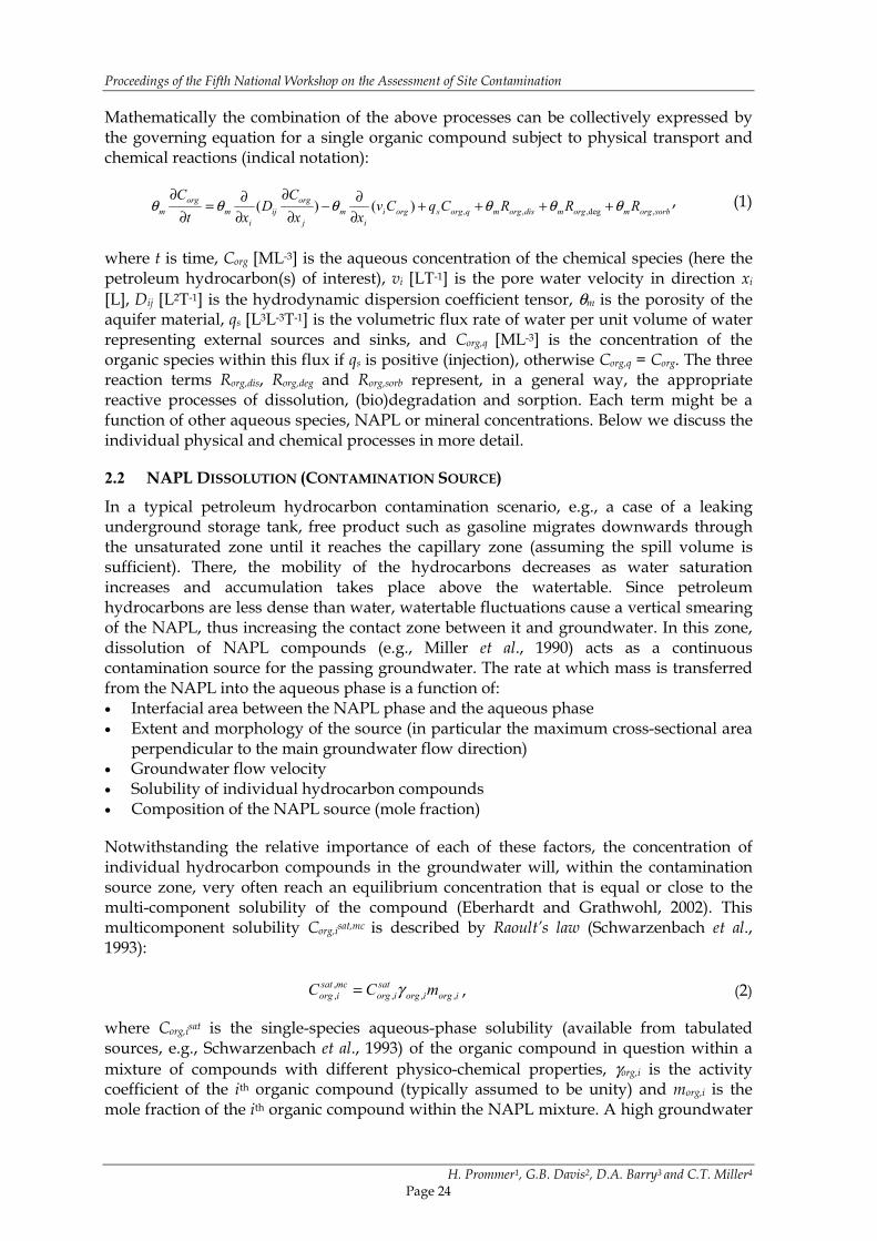
Mathematically the combination of the above processes can be collectively expressed bythe governing equation for a single organic compound subject to physical transport andchemical reactions (indical notation):

sorborgmorgmdisorgmqorgsorgii

mj

orgij

im

orgm RRRCqCv

xxC

Dxt

C,deg,,,)()( θθθθθθ ++++

∂∂−

∂∂

∂∂=

∂∂ , (1)

where t is time, Corg [ML-3] is the aqueous concentration of the chemical species (here thepetroleum hydrocarbon(s) of interest), vi [LT-1] is the pore water velocity in direction xi

[L], Dij [L2T-1] is the hydrodynamic dispersion coefficient tensor, θm is the porosity of theaquifer material, qs [L3L-3T-1] is the volumetric flux rate of water per unit volume of waterrepresenting external sources and sinks, and Corg,q [ML-3] is the concentration of theorganic species within this flux if qs is positive (injection), otherwise Corg,q = Corg. The threereaction terms Rorg,dis, Rorg,deg and Rorg,sorb represent, in a general way, the appropriatereactive processes of dissolution, (bio)degradation and sorption. Each term might be afunction of other aqueous species, NAPL or mineral concentrations. Below we discuss theindividual physical and chemical processes in more detail.

2.2 NAPL DISSOLUTION (CONTAMINATION SOURCE)

In a typical petroleum hydrocarbon contamination scenario, e.g., a case of a leakingunderground storage tank, free product such as gasoline migrates downwards throughthe unsaturated zone until it reaches the capillary zone (assuming the spill volume issufficient). There, the mobility of the hydrocarbons decreases as water saturationincreases and accumulation takes place above the watertable. Since petroleumhydrocarbons are less dense than water, watertable fluctuations cause a vertical smearingof the NAPL, thus increasing the contact zone between it and groundwater. In this zone,dissolution of NAPL compounds (e.g., Miller et al., 1990) acts as a continuouscontamination source for the passing groundwater. The rate at which mass is transferredfrom the NAPL into the aqueous phase is a function of:• Interfacial area between the NAPL phase and the aqueous phase• Extent and morphology of the source (in particular the maximum cross-sectional area

perpendicular to the main groundwater flow direction)• Groundwater flow velocity• Solubility of individual hydrocarbon compounds• Composition of the NAPL source (mole fraction)

Notwithstanding the relative importance of each of these factors, the concentration ofindividual hydrocarbon compounds in the groundwater will, within the contaminationsource zone, very often reach an equilibrium concentration that is equal or close to themulti-component solubility of the compound (Eberhardt and Grathwohl, 2002). Thismulticomponent solubility Corg,isat,mc is described by Raoult’s law (Schwarzenbach et al.,1993):

iorgiorgsat

iorgmcsatiorg mCC ,,,

,, γ= , (2)

where Corg,isat is the single-species aqueous-phase solubility (available from tabulatedsources, e.g., Schwarzenbach et al., 1993) of the organic compound in question within amixture of compounds with different physico-chemical properties, γorg,i is the activitycoefficient of the ith organic compound (typically assumed to be unity) and morg,i is themole fraction of the ith organic compound within the NAPL mixture. A high groundwater



Page 25

flow velocity, among other factors, might result in the kinetically–limited dissolution ofNAPL compounds. The simplest model that describes the concentration change of the ith

compound in groundwater is

)( ,,,, iorgmcsatiorgdisorg CCR −=ϖ , (3)

where Corg,i is the concentration of the ith organic compound in the groundwater and ϖ is amass-transfer rate coefficient that is a product of a mass transfer coefficient and thespecific interfacial area between NAPL phase and water. The combination of (2) and (3)applies to arbitrary dissolution rates. Note that ϖ approaches infinity for equilibriumdissolution. In that case Corg,i equals Corg,isat,mc .

2.3 ADVECTION AND DISPERSION

Once the hydrocarbon compounds have dissolved into the aqueous phase they are subjectto both advective and dispersive transport. In contrast to the unsaturated zone, masstransport in the saturated zone of the aquifer occurs mainly in the horizontal direction,i.e., the typical direction of groundwater flow. Within (1) advection and dispersion termsresult from averaging microscopic flow and transport processes occurring at the porescale within a representative elementary volume (REV), leading to a continuum model atthe macroscopic level (Bear, 1972). The advection term describes the transport of adissolved species transported at the same mean velocity as the groundwater, which is thedominant physical process in most field-scale contamination problems within the water–saturated groundwater zone. The dispersion term represents two processes, mechanicaldispersion and effective molecular diffusion. Mechanical dispersion results from thefluctuation of the (microscopic) streamlines in space with respect to the mean flowdirection and inhomogeneous conductivities within the REV. Molecular diffusion iscaused by the random movement of the molecules in a fluid. It is usually negligiblecompared to mechanical dispersion (Bear and Verruijt, 1987). The (macroscopic) porevelocity vi in (1) is derived from Darcy’s law (Darcy, 1856)

iji

j

K hvxθ∂= −∂

, (4)

and the three-dimensional flow equation for saturated groundwater (Bear, 1972):

thSq

xhK

x ssj

iji ∂

∂=+

∂∂

∂∂ , (5)

where Kij [LT-1] is the hydraulic conductivity tensor, h [L] is the hydraulic head and Ss [L-1]is the specific storativity. Note that the off-diagonal entries of the hydraulic conductivitytensor become zero if the principal components are aligned with the principal axes of theflow domain.

Analytical solution of the advection-dispersion equation exist only for relatively simplecases. Thus, for solving more complicated and realistic cases, e.g., involvingheterogeneous aquifers, transient boundary conditions, etc., numerical techniques such asthe Finite Difference and the Finite Element Methods (Pinder and Gray, 1977; Wang andAnderson, 1982; Bear and Verruijt, 1987; Istok, 1989) are required.



Page 26

2.4 SORPTION

Depending on the soil type, sorption, in particular to carbonaceous material (Miller andWeber, 1986, Grathwohl, 1990; Pedit and Miller, 1994, Allen-King et al., 2002), mightinfluence significantly aqueous concentrations of petroleum hydrocarbons. However, asindicated in Section 2.1, in most cases sorption kinetics mainly influences the time it takesfor petroleum hydrocarbon plumes to reach a steady-state length. At this stage,adsorption and desorption occur at the same rate and the sorption capacity of the soilgenerally does not influence the length of the plume, unless the flow-field is transient(Prommer et al., 2002). For quantification of the sorption process in a reactive transportmodel the rates at which the sorption reactions proceed dictate whether an equilibrium orkinetic sorption model is needed. An equilibrium model is appropriate if the sorptionreactions are fast compared to transport whereas in the case of a high flow-velocity and aslow sorption reaction a kinetic model might be required. In many cases slow sorptionand desorption is a result of intra-particle diffusion (Grathwohl et al., 2000; Eberhardt andGrathwohl, 2002). Models commonly used to quantify sorption at the field-scale are the:• Linear sorption equilibrium model• Freundlich nonlinear equilibrium model• Langmuir nonlinear equilibrium model

The linear model is the simplest and of the form (Farell and Reinhard, 1994)

orgDsorg CKC =, , (6)

where Corg,s is the sorbed concentration and KD is the partition coefficient, which dependsupon solid and solute properties (Karickhoff et al., 1979). The Freundlich model is(Grathwohl, 1998):

,Fn

org s F orgC K C= , (7)

where KF is the Freundlich sorption capacity coefficient, and nF is the Freundlich sorptionenergy coefficient (Freundlich, 1931; Weber, 1972). Although the literature reports valuesof nF between 0.7 and 1.8, typically it is less than and close to unity (Barry andBajracharya, 1995). The Langmuir model (Schwarzenbach et al., 1993) is

maxsorgorgL

orgLsorg C

CKCK

C ,,, 1+= , (8)

where KL is the (Langmuir) sorption monolayer capacity coefficient and Corg,s,max is theadsorption capacity. Note, that Corg,s and Corg,s,max are mass fractions, i.e., are defined as themass of an organic compound that is sorbed to a specific mass of soil [M M-1]. Of theabove models, the linear sorption equilibrium model is the simplest and perhaps mostcommonly used, especially for relatively low contaminant concentrations. However, itsinadequacy as a generally applicable model has been often demonstrated (Miller andWeber, 1984; 1986). The Freundlich model is also frequently used and adequatelydescribes most systems. Its power-law form leads to self-sharpening fronts for the typicalcase of nF < 1 and to increased complexity in the solution methods needed compared tothe linear case. The Langmuir model is applicable to cases in which sorption is limited to afinite capacity represented by, for example, a monolayer of solute coverage on the solidphase.



Page 27

In practice, i.e., when modelling a hydrocarbon plume at field-scale, it is usually verydifficult to identify, from measured data at the contaminated site, which model isappropriate in a particular case and decisions need to be made on the basis of results fromlaboratory batch or column experiments using soils-solid media from the specificcontaminated site.

2.5 BIODEGRADATION

Long-term, biodegradation will be the dominant process that decreases the total dissolvedmass within a plume generated by dissolution from NAPL sources. As dissolvedchemicals they are subject to both abiotic and biotic reactions. However, microbially-mediated (biotic) transformations are the major mechanism of contaminant removal asreaction rates are often accelerated by several orders of magnitude compared to abioticreaction rates (Schwarzenbach et al., 1993). The degradation of petroleum hydrocarbonsoccurs as a redox-reaction in which the hydrocarbons are oxidised at a significant rate if:• One or more aqueous electron acceptors such as O2, NO3-, SO42-, CO2 or electron

acceptors in mineral form are readily available,• A bacterial population capable of using the appropriate hydrocarbon compound is

present (at least at low concentration) or a population that can adapt itself to oxidisingthe hydrocarbon compound, and

• Basic nutrient requirements for the bacteria such as nitrogen, phosphorus or tracemetals are present.

Despite the acceleration of reaction rates by bacteria, in most cases the reactions arekinetically controlled, i.e., reactions do not proceed fast enough to allow the application ofequilibrium models. If multiple electron acceptors are involved in the biodegradation oforganic compounds, their consumption will typically be in the order of theirthermodynamic preference, i.e., in the order of decreasing Gibb’s free energy of thereaction, unless the electron accepting step is the rate-limiting step. This might happenindeed in the case of mineral form electron acceptors. If oxygen is present in an aquifer, itwill be consumed first, followed by nitrate. Under standard conditions iron-reduction or,occasionally, manganese-reduction might occur next (e.g., Stumm and Morgan, 1995),once nitrate is depleted. However, there are also cases where sulfate-reduction mightoccur first (Postma and Jakobsen, 1996) because the process is thermodynamically morefavourable or as a result of kinetic limitations of the dissolution of iron(III) minerals.During aerobic degradation and nitrate-, sulfate-, iron- and manganese-reduction thecarbon within the organic contaminants is converted, i.e., mineralised to inorganic carbon,typically in the form of (aqueous) CO2, but also to carbonate minerals such as calcite(CaCO3) or siderite (FeCO3), depending on the geochemical conditions. The CO2 producedfinally might serve itself as an electron acceptor whereby the carbon is partiallytransferred to methane (CH4).

A range of kinetic reaction models of differing complexity is available and has beenapplied in the past. The simplest way to mathematically describe the mass removal oforganic compounds due to biodegradation (with time) is to neglect any dependency of thetransformation rate of the organic substance on the concentration of other chemicals ormicrobial populations. Given these assumptions the most common kinetic degradationmodel is the first-order model (Bekins et al., 1998):

orgorg CkR 1deg, −= , (9)



Page 28

where k1 is a first-order biodegradation rate. This model assumes that the only factoraffecting the biodegradation rate is the concentration of substrate present; this may be thecase under some circumstances but very often is not. In particular the above-mentioneddependency of the biodegradation process on the presence of one or more electronacceptors is completely ignored by this model. Note that although the first-order modeloften fits reasonably well to data observed in the laboratory or in the field, the rateconstants (k1) obtained in the fitting process are generally not applicable for predictions atother sites with different hydrochemistry, organic compound mixtures, source zonegeometry, etc.

A simple model that takes into account the availability of one (dominant) electronacceptor was proposed by Borden et al. (1986). It assumes that an instantaneousbiodegradation reaction occurs where both substrate and electron acceptor are presentsimultaneously, i.e., that the reaction is limited only through the availability of either ofthe two reactants. Over a time step, ∆t, equations for the reactants on the left-hand sideare (Barry et al., 2002)

t

CR org

orgdeg ∆−=, if EA

EA

orgorg C

YY

C ≤ ,

t

CYY

R EA

EA

orgorgdeg ∆

−=, if EAEA

orgorg C

YY

C > , (10)

where CEA is the electron acceptor concentration and Yorg and YEA are stoichiometriccoefficients for the organic compound and the electron acceptor, respectively. The firstexpression in (10) is for the case when the contaminant concentration limits the reactionrate whereas the second applies when the electron acceptor concentration is limiting. Akey aspect of the instantaneous reaction model is that the concentration of at least one ofthe reacting species is zero for all times everywhere in the domain. In contrast to the first-order model, the instantaneous reaction model requires the simultaneous solution oftransport and reactions for the electron acceptor, i.e., the problem becomes a multi-speciestransport problem. For the instantaneous reaction model, the governing transportequation for the second species, the electron acceptor is:

sorbEAdegEAqEAs

EAiij

EAij

i

EA RRCqCvxx

CDxt

C,,,)()( +++

∂∂−

∂∂

∂∂=

∂∂

θ, (11)

where REA,deg and REA,sorb are the reaction terms that represent concentration changes due toorganic compound degradation and due to sorption, respectively.

The reaction term that results from the electron acceptor consumption duringbiodegradation is given by:

t

CYYR org

org

EAdegEA ∆

−=, if EAEA

orgorg C

YY

C ≤ ,

tCR EA

degEA ∆−=, if EA

EA

orgorg C

YY

C > , (12)

Lu et al. (1999) proposed an alternative simple reaction model that incorporates the rate-dependency on both organic substrate and electron acceptor availability. If only a single



Page 29

electron acceptor is considered, the first-order model in (9) might be replaced by one thatincorporates Michaelis-Menten type kinetics, leading to the degradation reaction term:

EAEA

EAorgdegorg CK

CCkR+

−= 1, , (13)

where KEA is the half-saturation constants of the electron acceptor. Another commonlyapplied model for the determination of the biodegradation term incorporates a doubleMichaelis-Menten term:

EAEA

EA

orgorg

orgdegorg CK

CCK

CkR

++−= 2, , (14)

where Korg is the half-saturation constant of the organic substance and k2 is a (pseudosecond-order) reaction constant. The corresponding reaction term for the electron acceptordiffers only by a constant factor that depends on the stoichiometry of the degradationreaction.

degorgorg

EAdegEA R

YYR ,, = , (15)

For example, for the degradation of toluene under sulfate-reducing conditions,

27 8 4 2 3 24.5 3 2 7 4.5C H SO H O H HCO H S− + −+ + + → + , (16)

the stoichiometric coefficients Yorg and YEA would be 1 and 4.5, respectively (if molarconcentrations are used), thus

degorgdegEA RR ,, 5.4= , (17)

As mentioned before, the biodegradation of petroleum hydrocarbons might involvemultiple electron acceptors that, typically, are used in a sequential manner. Accordingly,the number of transport equations that needs to be solved simultaneously increasesfurther. The appropriate degradation term for the organic compound proposed by Lu etal. (1999) then consists of the sum of individual terms for each step included in the (redox-sensitive) degradation process

42

42

32 ,,,,,, CHorgSOorgFeorgNOorgOorgdegorg RRRRRR ++++= −+− , (18)

where Rorg,O2, Rorg,NO3-, Rorg,Fe2+, Rorg,SO4-2 and Rorg,CH4 represent the contributions from aerobicdegradation, denitrification, iron-reduction, sulfate-reduction and methanogenesis,respectively. A common way of modelling the sequential consumption of electronacceptors in multi-species models is to introduce additional terms into (14), such thatREA,deg remains negligible in the presence of thermodynamically more favourable electronacceptors and such that only one of the individual terms on the RHS of (18) differssignificantly from 0 at a time. For example, organic compound degradation due todenitrification in the (occasional) presence of oxygen is then modelled as:



Page 30

−−

−

−− ++−=

33

3

22

2

33,

,,

NONO

NO

OOinh

OinhorgNONOorg CK

C

CKK

CkR , (19)

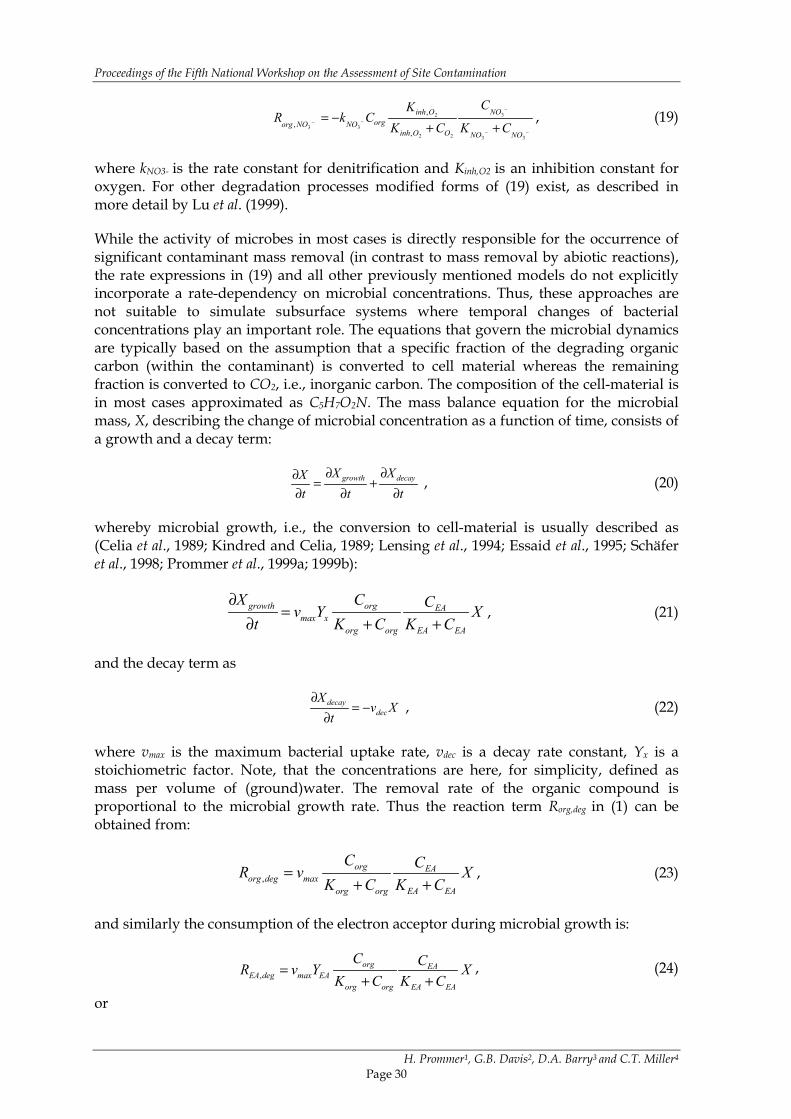
where kNO3- is the rate constant for denitrification and Kinh,O2 is an inhibition constant foroxygen. For other degradation processes modified forms of (19) exist, as described inmore detail by Lu et al. (1999).

While the activity of microbes in most cases is directly responsible for the occurrence ofsignificant contaminant mass removal (in contrast to mass removal by abiotic reactions),the rate expressions in (19) and all other previously mentioned models do not explicitlyincorporate a rate-dependency on microbial concentrations. Thus, these approaches arenot suitable to simulate subsurface systems where temporal changes of bacterialconcentrations play an important role. The equations that govern the microbial dynamicsare typically based on the assumption that a specific fraction of the degrading organiccarbon (within the contaminant) is converted to cell material whereas the remainingfraction is converted to CO2, i.e., inorganic carbon. The composition of the cell-material isin most cases approximated as C5H7O2N. The mass balance equation for the microbialmass, X, describing the change of microbial concentration as a function of time, consists ofa growth and a decay term:

tX

tX

tX decaygrowth

∂∂

+∂

∂=

∂∂ , (20)

whereby microbial growth, i.e., the conversion to cell-material is usually described as(Celia et al., 1989; Kindred and Celia, 1989; Lensing et al., 1994; Essaid et al., 1995; Schäferet al., 1998; Prommer et al., 1999a; 1999b):

growth org EAmax x

org org EA EA

X C Cv Y Xt K C K C

∂=

∂ + +, (21)

and the decay term as

Xvt

Xdec

decay −=∂

∂ , (22)

where vmax is the maximum bacterial uptake rate, vdec is a decay rate constant, Yx is astoichiometric factor. Note, that the concentrations are here, for simplicity, defined asmass per volume of (ground)water. The removal rate of the organic compound isproportional to the microbial growth rate. Thus the reaction term Rorg,deg in (1) can beobtained from:

,org EA

org deg maxorg org EA EA

C CR v XK C K C

=+ +

, (23)

and similarly the consumption of the electron acceptor during microbial growth is:

,org EA

EA deg max EAorg org EA EA

C CR v Y XK C K C

=+ +

, (24)

or



Page 31

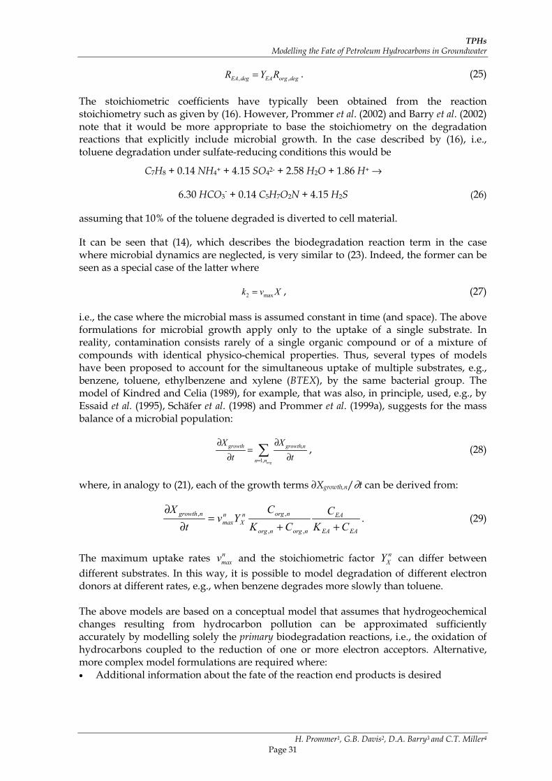
, ,EA deg EA org degR Y R= . (25)

The stoichiometric coefficients have typically been obtained from the reactionstoichiometry such as given by (16). However, Prommer et al. (2002) and Barry et al. (2002)note that it would be more appropriate to base the stoichiometry on the degradationreactions that explicitly include microbial growth. In the case described by (16), i.e.,toluene degradation under sulfate-reducing conditions this would be

C7H8 + 0.14 NH4+ + 4.15 SO42- + 2.58 H2O + 1.86 H+ →

6.30 HCO3- + 0.14 C5H7O2N + 4.15 H2S (26)

assuming that 10% of the toluene degraded is diverted to cell material.

It can be seen that (14), which describes the biodegradation reaction term in the casewhere microbial dynamics are neglected, is very similar to (23). Indeed, the former can beseen as a special case of the latter where

Xvk max2 = , (27)

i.e., the case where the microbial mass is assumed constant in time (and space). The aboveformulations for microbial growth apply only to the uptake of a single substrate. Inreality, contamination consists rarely of a single organic compound or of a mixture ofcompounds with identical physico-chemical properties. Thus, several types of modelshave been proposed to account for the simultaneous uptake of multiple substrates, e.g.,benzene, toluene, ethylbenzene and xylene (BTEX), by the same bacterial group. Themodel of Kindred and Celia (1989), for example, that was also, in principle, used, e.g., byEssaid et al. (1995), Schäfer et al. (1998) and Prommer et al. (1999a), suggests for the massbalance of a microbial population:

∑= ∂

∂=

∂∂

orgnn

ngrowthgrowth

tX

tX

,1

, , (28)

where, in analogy to (21), each of the growth terms ∂Xgrowth,n/∂t can be derived from:

EAEA

EA

norgnorg

norgnX

nmax

ngrowth

CKC

CKC

Yvt

X++

=∂

∂

,,

,, . (29)

The maximum uptake rates nmaxv and the stoichiometric factor n

XY can differ betweendifferent substrates. In this way, it is possible to model degradation of different electrondonors at different rates, e.g., when benzene degrades more slowly than toluene.

The above models are based on a conceptual model that assumes that hydrogeochemicalchanges resulting from hydrocarbon pollution can be approximated sufficientlyaccurately by modelling solely the primary biodegradation reactions, i.e., the oxidation ofhydrocarbons coupled to the reduction of one or more electron acceptors. Alternative,more complex model formulations are required where:• Additional information about the fate of the reaction end products is desired



Page 32

• The primary reactants are simultaneously involved in other reactions that proceedindependently (but at a comparable time-scale) or in response to the biodegradationreactions.

The former point is of particular interest for applying natural attenuation as a remediationscheme. There, the geochemical changes resulting from the biodegradation reactions areused to demonstrate the occurrence of attenuation processes (Wiedemeier et al., 1995).Where the contaminants (e.g., BTEX) are oxidised, this typically includes changes inalkalinity, total inorganic carbon (TIC) and of reduced forms of electron acceptors such assulfide or ferrous iron. These and other species might undergo further reactions, e.g., theycan form mineral precipitates such as siderite (FeCO3), iron sulfide (FeS) or pyrite (FeS2).The question whether these (secondary) reactions proceed and, if so, at what rate, is moredifficult to solve than the more simple cases presented above. The occurrence and rate ofthese reactions depend, for example, on the pH of the groundwater, which itself changesduring biodegradation of organic contaminants. In such cases, the reaction terms within(1) are functions of a large number of chemicals (aqueous species, minerals, etc) andgeochemical models that are based on thermodynamic principles are typically used tocompute those terms. Among the biodegradation models that include geochemicalreactive processes, two different approaches are commonly used to formulate thebiodegradation reactions. Brun et al. (2002) classified biogeochemical models into:• Single-step process models, where the oxidation of the organic compound and the

electron-accepting step proceed as a single redox reaction at a specific rate, or• Two-step process models in which it is assumed that the oxidation step is the rate-

limiting step and where the electron-accepting step can (but does not have to) bemodelled as an equilibrium reaction. The electron-acceptor(s) used duringdegradation of one or more organic compounds are not defined a priori, butconsumed according to their thermodynamic favourability.

Both types of the above biogeochemical transport models are, at present, not appliedroutinely for the simulation of hydrocarbon pollution problems. However, they areincreasingly applied in research projects that aim at an improved understanding ofnatural and enhanced remediation processes (e.g., Schäfer et al., 2002; Brun et al., 2002;Prommer et al., 2002). Further details on the fundamentals of the (underlying) theory ofmulticomponent reactive transport can be found for example in Yeh and Triphati (1989)and Steefel and MacQuarrie (1996).

3 NUMERICAL MODELLING

The above mathematical descriptions of physical, chemical and biological processes needfor all but the most trivial cases to be incorporated into and solved by numerical models.Below we discuss the steps that are most-often involved in numerical modelling ofpetroleum hydrocarbon contaminated sites and mention some of the most commonlyused modelling tools. An example case is also presented. In tandem with modelling is aprocess of data gathering, starting with basic background site data, to characterisationdata on contaminant distributions, to more detailed measurements depending on theintent of the modelling. This procedure is evident, for example, in Davis et al. (1993) andDavis et al. (1999).

The application of numerical models of subsurface flow such as MODFLOW (McDonaldand Harbaugh, 1988), HST3D (Kipp, 1986), FEMWATER (Yeh et al., 1992) or FEFLOW



Page 33

(Diersch, 1997) which incorporate information on the hydrological and hydrogeologicalproperties and which can simulate the groundwater flow at a site will typically form thebasis for subsequent contaminant transport simulations. It is also the most important step,as any discrepancy between the flow model and reality will be propagated to thetransport model. In many cases, a proper groundwater flow model itself can alreadyprovide useful information. The flow modelling step provides a process-basedinterpretation and interpolation of the hydraulic heads recorded at observation wells. Itmight be used for the delineation of (sub-) catchments, capture zones (e.g., of extractionwells) and for the development of a model-based design of purely hydraulic remediationmeasures (e.g., pump and treat designs). Add-on packages of flow models that simulatepurely advective transport might be used for the prediction of the flow path of a plumecentre and to estimate how fast the leading edge of a contamination would migrate in anon-reactive case, i.e., if no biodegradation or sorption occurred. The latter point, however,concerns only the early stages of a pollution problem (Stage 1). Modelling packages suchas PMPATH (Chiang and Kinzelbach, 2000) or MODPATH (Pollock, 1994) allowpredictions of the contaminant flow path and travel times of non-reactive contaminantsusing particle-tracking algorithms.

The first step in building a site-specific groundwater flow model is, based on apreliminary site characterisation, the development of a conceptual hydrological andhydrogeological model. At this stage, all available geologic and hydrographic informationis collated and analysed. The conceptual model formulates qualitatively:• The general groundwater flow direction;• Boundaries that might be used as boundaries in the numerical model, such as

(subsurface) catchment boundaries and (dividing) streamlines;• Which stratigraphic layer(s) are more and which ones are less or much less permeable,

which layer(s) are suitable to form a boundary in the numerical model; and• The fluxes into and out of a chosen (model) domain and how to determine/estimate

these fluxes quantitatively.

The conceptual model needs then to be translated into a numerical model by:• Spatially discretising the model domain;• Allocating measured or estimated hydrogeological aquifer parameters such as

conductivity or porosity;• Allocating/defining initial, starting values, e.g., hydraulic heads;• Allocating/defining static or time-dependent boundary conditions, e.g., recharge; and• Model calibration using observed/monitored data (e.g., hydraulic heads) by variation

of parameters for values that are not well known.

Details of this procedure can be found in many groundwater hydrology specific textbookssuch as by Freeze and Cherry (1979) or Fetter (1999) or, more modelling specific texts suchas that by Anderson and Woessner (1992) and Chiang and Kinzelbach (2000).

3.1 NON-REACTIVE TRANSPORT MODELLING

Based on a (calibrated) groundwater flow model, the next step in a sound modellingstudy is a non-reactive advective-dispersive transport model. In particular, if one or moreof the organic compounds are recalcitrant to biodegradation (or apparently degrading atslow rates), monitoring data for this compound can be used to quantify, i.e., estimate orcalibrate the transversal dispersivity of the aquifer, a key parameter that has a controlling



Page 34

influence on the length of a contaminant plume. Other important roles of the non-reactivemodel might be:• Identification of errors in the data and parameter preparation/allocation; and• Identification of the extent dilution might be responsible for a decrease in pollutant

concentrations downstream of a contamination source

Note that the conceptual model (for example the dimensionality of the model) might notneed to be the same as in the flow model. For example, a cross-sectional transport modelmight be constructed along a flow path that was determined in the previous(flow/particle tracking) step.

In principle a wide range of different transport models are suitable for this step. However,over a number of years the MODFLOW-based transport simulator MT3D (Zheng, 1990)has evolved as a quasi-standard groundwater transport model. The reason for this beingits modular construction, its robustness and its good documentation, including sourcecode availability. Consequently, it is used by several reactive transport simulators thatemploy the (newer) multi-species version MT3DMS (Zheng and Wang, 1999) as a modulefor simulating advective-dispersive transport.

3.2 BIODEGRADATION MODELLING

The above-mentioned extension of the original single-species transport code MT3D to themulti-species transport simulator MT3DMS provided the starting point for thedevelopment of a number of models that simulate coupled hydrological transport ofmultiple chemical species and the chemical reactions among these species. For example,RT3D (Clement, 1997) couples the implicit ordinary differential equation (ODE) solverLSODA to solve arbitrary kinetic reaction problems. RT3D provides a number of pre-defined reaction packages, e.g., for biodegradation of oxidisable contaminants consumingone or more electron acceptors. However, most importantly, users can also define theirown reaction packages in order to adapt the numerical model to a site-specific conceptualhydrochemical model. This means that “non-standard” kinetic rate formulations forbiodegradation reactions, as per some of the model formulations presented in Section 2.5,can be implemented reasonably quickly into the RT3D model. Other MT3D/MT3DMS-based reactive transport models that simulate the fate of specific pollutants, includingBTEX, by solving purely kinetic biodegradation reactions, i.e., the primary biodegradationreactions, are listed in Table 1. Of course, non-MT3DMS based biodegradation models doalso exist. However, many of them lack integration into a suitable, user-friendly graphicalenvironment, making them less useful for routine applications.

Table 1: Examples of available biodegradation modelsModel ReferenceRT3D Clement (1997)

MT3D99 SSPA (1999), http://www.sspa.comBIOREDOX Carey et al. (1999)

SEAM3D Waddill and Widdowson (1998)

Multispecies biodegradation models require the definition of initial and boundaryconditions for each species included. In most cases the initial conditions are defined bythe concentrations of the unpolluted zone (background concentrations). Modelling of thepollution source can be handled in various ways, for example as:



Page 35

• A mass transfer (dissolution) process as indicated in Section 2.2;• A fixed concentration boundary condition, i.e., the contaminant concentration in the

source area is fixed; and• A flux boundary condition where the contaminant is added to the aquifer at a

predefined mass per unit time, independent of the actual groundwater flow velocity.

The first option will typically provide the solution that reflects best the processes at acontaminated site. More details on applied reactive transport modelling are given in, e.g.,Zheng and Bennett (2002).

3.3 BIOGEOCHEMICAL MODELLING

A range of numerical simulators is available that can simultaneously account for bothbiodegradation and geochemical reactions. In contrast to the above-mentionedbiodegradation models, the transport equation in so-called ‘multi-species’ models istypically not solved separately for each chemical species but for total aqueous componentconcentrations (e.g., Yeh and Tripathi, 1989; Steefel and MacQuarrie, 1996). While it is notpossible here to discuss the relative merits of each of the simulators, a list of suitablemodels for these types of applications is given in Table 2.

Table 2: Examples of available biogeochemical transport modelsModel ReferenceCRUNCH Steefel and Yabusaki (1996), Steefel (2001)PHT3D Prommer et al. (2002, 2003)PHAST Parkhurst et al. (1995)MIN3P Mayer (1999)TBC Schäfer et al. (1998)HBGC123D Salvage (1998), Salvage and Yeh (1998)

3.4 PRE- AND POST-PROCESSING TOOLS

For routine model applications pre- and post-processing of model input and output datamight comprise the majority of effort for a modelling exercise. Over the past few yearssignificant advances have been made in incorporating GIS-type features into the mostcommonly used graphical user interfaces (GUIs), as well as with respect to rapid three-dimensional visualisation. A list of the most popular GUIs is given in Table 3. No attemptwas made to rate them, as the suitability of each product depends on a range of factorssuch as available hardware and whether the GUI supports a specific biodegradationmodel.

Table 3: Most commonly used GUIs for MODFLOW/MT3D based flow and transport modelsGUI Reference

PMWIN http://www.iesinet.comChiang and Kinzelbach (2000)

Visual Modflow http://www.visual-modflow.comGMS http://www.ems-i.com

Groundwater Vistas http://www.groundwater-vistas.comArgus ONE http://www.argusint.com



Page 36

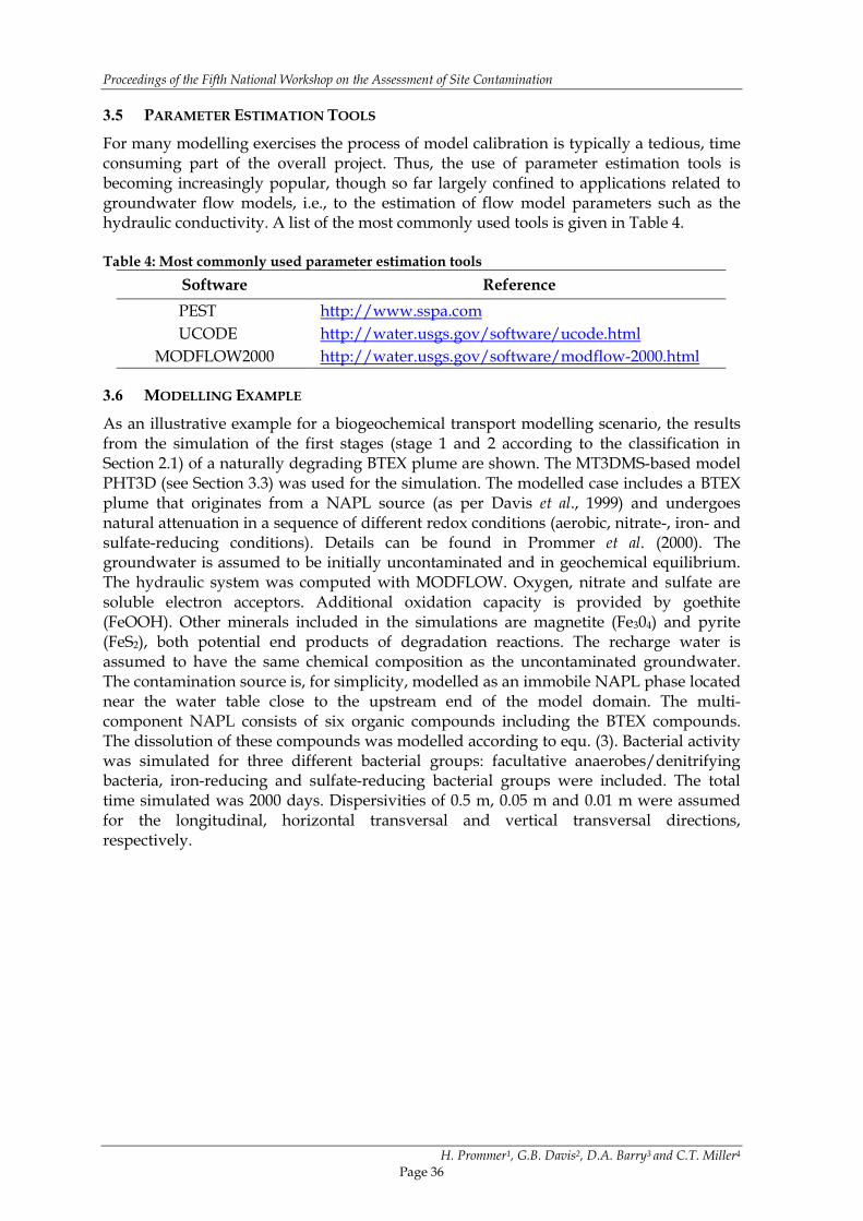
3.5 PARAMETER ESTIMATION TOOLS

For many modelling exercises the process of model calibration is typically a tedious, timeconsuming part of the overall project. Thus, the use of parameter estimation tools isbecoming increasingly popular, though so far largely confined to applications related togroundwater flow models, i.e., to the estimation of flow model parameters such as thehydraulic conductivity. A list of the most commonly used tools is given in Table 4.

Table 4: Most commonly used parameter estimation toolsSoftware ReferencePEST http://www.sspa.comUCODE http://water.usgs.gov/software/ucode.html

MODFLOW2000 http://water.usgs.gov/software/modflow-2000.html

3.6 MODELLING EXAMPLE

As an illustrative example for a biogeochemical transport modelling scenario, the resultsfrom the simulation of the first stages (stage 1 and 2 according to the classification inSection 2.1) of a naturally degrading BTEX plume are shown. The MT3DMS-based modelPHT3D (see Section 3.3) was used for the simulation. The modelled case includes a BTEXplume that originates from a NAPL source (as per Davis et al., 1999) and undergoesnatural attenuation in a sequence of different redox conditions (aerobic, nitrate-, iron- andsulfate-reducing conditions). Details can be found in Prommer et al. (2000). Thegroundwater is assumed to be initially uncontaminated and in geochemical equilibrium.The hydraulic system was computed with MODFLOW. Oxygen, nitrate and sulfate aresoluble electron acceptors. Additional oxidation capacity is provided by goethite(FeOOH). Other minerals included in the simulations are magnetite (Fe304) and pyrite(FeS2), both potential end products of degradation reactions. The recharge water isassumed to have the same chemical composition as the uncontaminated groundwater.The contamination source is, for simplicity, modelled as an immobile NAPL phase locatednear the water table close to the upstream end of the model domain. The multi-component NAPL consists of six organic compounds including the BTEX compounds.The dissolution of these compounds was modelled according to equ. (3). Bacterial activitywas simulated for three different bacterial groups: facultative anaerobes/denitrifyingbacteria, iron-reducing and sulfate-reducing bacterial groups were included. The totaltime simulated was 2000 days. Dispersivities of 0.5 m, 0.05 m and 0.01 m were assumedfor the longitudinal, horizontal transversal and vertical transversal directions,respectively.



Page 37

121416

Cross-section along plumes Cross-sections across plumes

m0 20 40

Benzene (mg/l)

121416

m

0 20 40

Toluene (mg/l)

121416

m

0 2 4

Oxygen (mg/l)

121416

m

0 10 20 30

Nitrate (mg/l)

121416

m

100120140

Sulphate (mg/l)

121416

m

0 50 100

Goethite (mg/l)

121416

m

6 7 8

pH

121416

m

-5 0 5 1015

pe

121416

m

120 160

C(IV) (mg HCO3 - )

121416

m

0 50 100

Magnetite (mg Fe/l)

121416

m

0 10 20

Pyrite (mg Fe/l)

121416

m

-7 -6 -5

Aerob./Denitr. log(mol/l)

121416

m

-7 -6 -5

Fe(III) reducer log(mol/l)

50 100 150 200 250

121416

m

m

-7 -6 -5

Sulph. reducer log(mol/l)

Figure 2. Concentrations of hydrocarbon compounds (e.g., benzene, toluene), electron acceptors(e.g., oxygen, sulfate), mineral phases (e.g., geothite), and bacterial groups (e.g.,aerobic/denitrifiers) after a simulation time of 800 days. Cross sections along theplumes are for the plume centreline; half cross sections across the plumes are shownfor x = 52.5 m, which is 33 m downgradient of the NAPL source.

Figure 2 summarises some of the output from the simulation. Once dissolved from theNAPL source, the organic compounds migrate downstream while being either partly orcompletely degraded by a series of biogeochemical reactions. Due to their higher (multi-component) solubility, only the BTEX compounds reach significant concentrations in thedissolved phase (see benzene and toluene plot in Figure 2, other compounds are notshown). Driven by aquifer recharge, the plume centre moves downward toward the baseof the aquifer with increasing distance. After 2 years, the mass of dissolved toluene peaks



Page 38

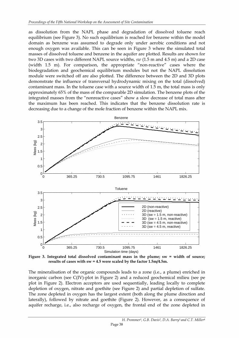
as dissolution from the NAPL phase and degradation of dissolved toluene reachequilibrium (see Figure 3). No such equilibrium is reached for benzene within the modeldomain as benzene was assumed to degrade only under aerobic conditions and notenough oxygen was available. This can be seen in Figure 3 where the simulated totalmasses of dissolved toluene and benzene in the aquifer are plotted. Results are shown fortwo 3D cases with two different NAPL source widths, sw (1.5 m and 4.5 m) and a 2D case(width 1.5 m). For comparison, the appropriate “non-reactive” cases where thebiodegradation and geochemical equilibrium modules but not the NAPL dissolutionmodule were switched off are also plotted. The difference between the 2D and 3D plotsdemonstrate the influence of transversal hydrodynamic mixing on the total (dissolved)contaminant mass. In the toluene case with a source width of 1.5 m, the total mass is onlyapproximately 65% of the mass of the comparable 2D simulation. The benzene plots of theintegrated masses from the “nonreactive cases” show a slow decrease of total mass afterthe maximum has been reached. This indicates that the benzene dissolution rate isdecreasing due to a change of the mole fraction of benzene within the NAPL mix.

0 365.25 730.5 1095.75 1461 1826.250

0.5

1

1.5

2

2.5

3

3.5

Mas

s (k

g)

Benzene

0 365.25 730.5 1095.75 1461 1826.250

0.5

1

1.5

2

2.5

3

3.5

Mas

s (k

g)

Simulation time (days)

Toluene

2D (non-reactive)2D (reactive)3D (sw = 1.5 m, non-reactive)3D (sw = 1.5 m, reactive)3D (sw = 4.5 m, non-reactive)3D (sw = 4.5 m, reactive)

Figure 3. Integrated total dissolved contaminant mass in the plume; sw = width of source;results of cases with sw = 4.5 were scaled by the factor 1.5m/4.5m.

The mineralisation of the organic compounds leads to a zone (i.e., a plume) enriched ininorganic carbon (see C(IV)-plot in Figure 2) and a reduced geochemical milieu (see peplot in Figure 2). Electron acceptors are used sequentially, leading locally to completedepletion of oxygen, nitrate and goethite (see Figure 2) and partial depletion of sulfate.The zone depleted in oxygen has the largest extent (both along the plume direction andlaterally), followed by nitrate and goethite (Figure 2). However, as a consequence ofaquifer recharge, i.e., also recharge of oxygen, the frontal end of the zone depleted in



Page 39

oxygen does not travel as fast as the zone enriched in inorganic carbon. Aerobicdegradation and reduction of nitrate cause a decrease in pH whereas pH increases underiron- and sulfate-reducing conditions. In the model scenario presented, a low pH zone iscreated only at the front of the “reactive zone” (Figure 2), whereas in the rest of the“reactive zone” an increased pH is found. In the model scenario presented, magnetite isthe dominant iron species where goethite has been reduced, however, some reduced ironreacts with the sulfide produced in the sulfate-reducing zone and precipitates as pyrite(Figure 2).

The plots for the simulated bacterial concentrations indicate the locations of ongoingdegradation and the appropriate dominant reduction reactions. As can be seen in theappropriate plots for aerobes/denitrifying and for iron-reducing bacteria (Figure 2), thebacterial activity related to locally completely depleted components/minerals is confinedto the fringes of these zones. However, as oxygen and nitrate are replenished fromupstream, the contamination source zone is the most active zone while the iron-reducingzone travels downstream. Sulfate-reducing bacteria dominate within the inner plume corewhere all other electron acceptors except sulfate have been depleted.

4 SUMMARY AND PRACTICAL IMPLICATIONS

Modelling the fate of petroleum hydrocarbons in groundwater consists of a series ofsequential steps. Of course, each site has its own characteristics with respect to the:

• contaminant composition/mixture;• contamination history and available details of this history;• availability of hard and soft data;• hydrogeology; and• hydrochemistry and mineralogy.

and thus the modelling methodology will need to be adapted to individual, site-specificrequirements.

However, the steps listed in Table 5 might serve as a general guideline/checklist thatprovides a basis for a site-specific schedule of a modelling study.

The importance of a correct conceptual model of flow characteristics and biogeochemicalinteractions must be highlighted again. Ideally, each of the modelling steps needs testingand validation against data from the site. On the other hand, if modelling is carried out atan early stage during the assessment of a contaminated site its main role might be theidentification of gaps in available data (or knowledge in general) for a site or thebehaviour of a specific contaminant.

Note, that not all the steps outlined in Table 5 may be required and/or feasible in allmodelling studies. However, consideration of each step is recommended where fullbiogeochemical modelling assessments are to be carried out. As the basis for allsubsequent steps, a sound conceptual understanding and model for a site is fundamental,as is adequate site data to translate such a conceptual model into a formalised modellingframework as outlined here.



Page 40

Table 5: Checklist of major steps in a reactive transport modelling studyStep Activity

1 Initial assessment of the existing data/situation to be modelled – initialidentification of potential physical and chemical interactions including initial ‘hand’calculations of flow rates and initial ‘electron balance’, where possible.

2 Compilation of a first conceptual model for the contaminated site.In particular, detailed depth profile data (from multi-level sampling devices) canhelp formulate the conceptual model for a site. Care is needed as to the sourceconditions for the plume source – NAPL concentrations, source dimensions. Theywill strongly influence plume characteristics and the longevity of the contaminationsource.

3 Formulation of a modelling strategy (dimensionality, spatial and temporalresolution, process-detail of modelled physical and chemical processes) andformulation of the questions that the model(s) will need to answer.When deciding upon the process detail of the chemical processes, i.e., the reactionmodel, remember that:Components of petrol products, including benzene, toluene, ethylbenzene,naphthalene, etc do not degrade at similar rates or under similar geochemicalconditions – for example, often toluene will degrade more readily than benzene; andZero-, first-order or any non-specific third-party reaction rate should only be usedwhere groundwater and aquifer mineral geochemical signatures are similar.

4 Selection of appropriate modelling tools, depending on available data, questions tobe answered and available time.

5 Setup of a flow model, including spatial discretisation of the model domain into gridcells, definition of boundary conditions, temporal discretisation of the simulationperiod, e.g., to account for seasonal recharge dynamics, time stepping, data input.

6 Data preparation of observation data to allow for comparison with simulationresults during flow model calibration.

7 Calibration of steady state or transient flow model using existing observations ofhydraulic heads. Model calibration might be carried out by hand (trial-and-error) orusing parameter estimation tools.

8 Testing of the plausibility of simulated flow velocities, flow path and water budgets.

9 Ideally (though in most cases not feasible) application/testing of the model for datathat have not been used during model calibration.

10 Identification of data gaps which hamper the reliability of the calibrated model.Preparation of plans for acquisition of additional data, where feasible.

11 Setup of a transport model for advective/dispersive non-reactive transport of asingle species.Note, that the model domain of the transport model might be a sub-domain of theflow model and that the model might have a different dimensionality.

12 Initial model runs of the above single-species model to assess and fix numericalproblems that result from pure physical transport (e.g., convergence problems,oscillations, numerical dispersion).

13 Crude adjustment of (longitudinal and transversal) dispersivity values to governmajor plume characteristics.

14 Use of initial transport modelling results as a (further) plausibility control for theflow model.For example, a conservative, i.e., non-reactive species (tracer) in the model should



Page 41

Step Activitytravel approximately at the conceptual groundwater flow velocity. Where necessary,adjustments of the conceptual and numerical flow model.

15 If existing reaction modules appear unsuitable – preparation of a site-specificreaction module, testing of the reaction module/package for simplistic, non site-specific flow configurations.

16 Data preparation of observation data to allow for comparison with simulationresults during transport model calibration.

17 If a multi-component reactive transport model is employed –- Batch-typegeochemical equilibrium modelling of background water chemistry to assessaqueous phase – mineral equilibria of the uncontaminated aquifer. Batch-typereaction simulations to assess geochemical changes in response to the mineralisationof hydrocarbons.

18 Setup of multi-species, multi-component transport model, including first estimateof reaction parameters (from literature), where necessary.

19 Biogeochemical transport modelling simulations. Adjustment of reaction parametersto match observed plume patterns – Plume length/concentrations of hydrocarbons,redox zonation/concentrations of dissolved electron acceptors, occurrence ofreaction products.

20 Sensitivity analysis of calibrated model.

21 Computation of detailed mass budgets for dissolved species/components.

22 Predictive model runs to (i) estimate the long-term contaminant plume evolutionand the associated risk for receptors (ii) answer ‘what if’ – type questions.Estimates of future stresses are needed to perform a predictive simulationCare is needed when deciding on ‘future’ source conditions for predictive runs – thedistribution and composition of NAPL may be highly variable depending on itsweathered status and the location of the water table in the subsurface.Note – assuming a large lateral dispersivity can lead to predictions of short plumesdue to unrealistic (over-predicted) mixing/dilution of reactants (hydrocarbons andelectron acceptors) and inducement of biodegradation in those zones.

23 Reporting and documenting the modelling study

5 ACKNOWLEDGEMENT

This publication has partially arisen from the Corona project. Corona is a research projectsupported by the European Commission under the Fifth Framework Programme andcontributing to the implementation of Key Action 1 'Sustainable Management and Qualityof Water' within the thematic programme for Energy, Environment and SustainableDevelopment.



Page 42

REFERENCES

Alexander M (1994) Biodegradation and bioremediation, p. 71-98. Academic Press, A division ofHarcourt Brace & Company, New York.

Allen-King RM, Grathwohl P, Ball WP (2002) New modeling paradigms for the sorption ofhydrophobic organic chemicals to heterogeneous carbonaceous matter in soils, sedimentsand rocks. Adv. Wat. Resour. 25, 985-1016.

Anderson MP, Woessner WW (1992) Applied Groundwater Modeling Simulation of Flow and AdvectiveTransport. Academic Press.

Barry DA, Bajracharya K (1995) Muskingum-Cunge solution method for solute transport withequilibrium Freundlich reactions. J. Contam. Hydrol. 18, 221-238.

Barry DA, Prommer H, Miller CT, Engesgaard P, Brun A, Zheng C (2002) Modelling the fate ofoxidisable organic contaminants in groundwater. Adv. Water. Resour. 25, 899-937.

Bear J (1972) Dynamics of Fluids in Porous Media. Dover Publications Inc., New York.

Bear J, Verruijt A (1987) Modeling Groundwater Flow and Pollution. D. Reidel Publishing Co.

Bekins BA, Warren E, Godsy EM (1998) A Comparison of zero-order, first-order, and Monodbiotransformation models, Ground Water 36, 261-268

Borden RC, Bedient PB, Lee MD, Ward CH, and Wilson JT (1986) Transport of dissolvedhydrocarbons influenced by oxygen-limited biodegradation, 2. field application. WaterResour. Res. 22, 1973-1982.

Brun A, Engesgaard P, Christensen TH, Rosbjerg D (2002) Modelling of transport andbiogeochemical processes in pollution plumes: Vejen landfill, Denmark. J. Hydrol. 256, 228-247.

Carey GR, Van Geel PJ, Murphy JR (1999) BIOREDOX-MT3DMS: A coupled biodegradation-redoxmodel for simulating natural and enhanced bioremediation of organic pollutants. Version2.0 User’s guide. Conestoga-Rovers & Associates, Waterloo Canada.

Celia MA, Kindred JS, Herrera I (1989) Contaminant transport and biodegradation: 1. a numericalmodel for reactive transport in porous media. Water Resour. Res. 25, 1141-1148.

Chiang W-H, Kinzelbach W (2000) 3D-Groundwater modeling with PMWIN: A Simulation System forModeling Groundwater Flow and Pollution. Springer-Verlag.

Clement TP (1997) RT3D - A Modular Computer Code for Simulating Reactive Multi-species Transport in3-Dimensional Groundwater Aquifers. Battelle Pacific Northwest National Laboratory ResearchReport, PNNL-SA-28967.

Darcy, H (1856) Les Fontaines Publiques de la Ville de Dijon. Dalmont, Paris.

Davis GB, Barber C, Power TR, Thierrin J, Patterson BM, Rayner, JL, Wu Q (1999) The variability andintrinsic remediation of a BTEX plume in anaerobic sulfate-rich groundwater. J. Contam.Hydrol. 36, 265-290.

Davis GB, Johnston CD, Thierrin J, Power TR, Patterson BM (1993) Characterising the distribution ofdissolved and residual NAPL petroleum hydrocarbons in unconfined aquifers to effectremediation. AGSO Journal of Australian Geology & Geophysics 14, 243-248.

Diersch H-JG (1997) Interactive, Graphics-based Finite-Element Simulation System FEFLOW forModelling Groundwater Flow. Contaminant Mass and Heat Transport Processes. User’s ManualVersion 4.6. WASY. Institute for Water Resources Planning and System Research Ltd., Berlin.



Page 43

Eberhardt C, Grathwohl, P (2002) Time scales of organic contaminant dissolution from complexsource zones: coal tar pools vs. blobs. J Contam. Hydrol. 59, 45-66.

Essaid HI, Bekins BA, Godsy EM, Warren E, Baedecker MJ, Cozarelli IM (1995). Simulation ofaerobic and anaerobic biodegradation processes at a crude-oil spill site. Water Resour. Res. 31,3309-3327.

Farrell J, Reinhard M (1994) Desorption of halogenated organics from model solids, sediments, andsoil under unsaturated conditions. 1. Isotherms. Environ. Sci. Technol. 28, 53-62.

Fetter CW (1999) Contaminant Hydrogeology, 2nd ed. Prentice Hall Publishers.

Freeze RA, Cherry JA (1979) Groundwater. Prentice-Hall, N.J.

Freundlich H (1931) Of the adsorption of gases. section II. kinetics and energetics of gas adsorption.J. American Chemi. Soc. 195-201.

Grathwohl P (1990). Influence of organic matter from soils and sediments from various origins onthe sorption of some chlorinated aliphatic hydrocarbons: implications of Koc correlations.Environ. Sci. Technol. 24, 1687-1693.

Grathwohl P (1998) Diffusion in Natural Porous Media: Contaminant Transport, Sorption/Desorption andDissolution Kinetics. Topics in Environmental Fluid Mechanics. Kluwer, Boston.

Grathwohl P, Klenk ID, Eberhardt C, Maier U (2000) Steady state plumes: mechanisms oftransverse mixing in aquifers. In: Contaminated Site Remediation: From Source Zones toEcosystems (ed. by C.D. Johnston), Proc. 2000 Contaminated Site Remediation Conference,Melbourne, 4-8 December 2000, 459-466.

Imhoff PT, Jaffé PR, Pinder GF (1993) An experimental study of the complete dissolution of anonaqueous phase liquid in saturated porous media. Water Resour. Res. 30, 307-320.

Istok JD (1989) Groundwater Modeling by the Finite Element Method. American Geophysical Union,Water Resources Monograph; 13.

Karickhoff SW, Brown DS, Scott TA (1979) Sorption of hydrophobic pollutants on naturalsediments. Water. Res. 13, 241-248.

Kipp KL, Jr (1986) HST3D-A Computer Code for Simulation of Heat and Solute Transport in 3D Ground-Water Flow Systems. U.S. Geological Survey Water-Resources Investigations Report 86-4095.

Kindred JS, Celia MA (1989) Contaminant transport and biodegradation: II. Conceptual model andtest simulations. Water Resour. Res. 25, 1149-1160.

Lensing HJ, Vogt M, Herrling B (1994) Modeling of biologically mediated redox processes in thesubsurface. J. Hydrol. 159, 125-143.

Lu G, Clement TP, Zheng C, Wiedemeier TH (1999) Natural attenuation of BTEX compounds,model development and field-scale application. Ground Water 37, 707-717.

Mayer KU (1999) A numerical model for multicomponent reactive transport in variably saturatedporous media. PhD Thesis, Department of Earth Sciences, University of Waterloo.

McDonald JM, Harbaugh AW (1988) A Modular 3D Finite Difference Ground-Water Flow Model.Technical report, U.S. Geological Survey techniques of Water-Resources Investigations.

Miller CT, Poirier-McNeill MM and Mayer AS (1990) Dissolution of trapped nonaqueous phaseliquids: Mass transfer characteristics. Water Resour. Res. 26, 2783-2796.

Miller CT, Weber Jr WJ (1984) Modeling organic contaminant partitioning in ground watersystems. Ground Water 22, 584-592.



Page 44

Miller CT, Weber Jr WJ (1986) Sorption of hydrophobic organic pollutants in saturated soilsystems. J. Contam. Hydrol. 1, 243-261.

Parkhurst DL, Engesgaard P, Kipp KL (1995) Coupling the geochemical model PHREEQC with a3D multi-component solute transport model. In Fifth Annual V.M. Goldschmidt Conference,Penn State University, University Park Pennsylvania, USA, May 1995.

Parkhurst DL, Appelo CAJ (1999) User’s guide to PHREEQC – A computer program for speciation,reaction-path, 1D-transport, and inverse geochemical calculations: Technical Report 99-4259,US Geol. Survey Water-Resources Investigations Report.

Pedit, JA, Miller CT. (1994) Heterogeneous sorption processes in subsurface systems, 1. Modelformulations and applications. Env. Sci. Technol. 28, 2094-2104.

Pinder GF, Gray WG (1977) Finite Element Simulation in Surface and Subsurface Hydrology. AcademicPress, London, 295 pp.

Pollock DW (1994) User's Guide for MODPATH/MODPATH-PLOT, Version 3: A Particle TrackingPost-processing Package for MODFLOW, the U.S. Geological Survey Finite-difference Ground-waterFlow Model. U.S. Geological Survey Open-File Report 94-464, 234 p.

Postma D, Jakobsen R (1996) Redox zonation: equilibrium constraints on the Fe(III)/SO4-reductioninterface. Geochim. Cosmochim. Acta, 60, 3169-3175.

Prommer H (2002a) PHT3D – A Reactive Multicomponent Transport Model for Saturated Porous Media.User’s Manual Version 1.0. Technical report of Contaminated Land Assessment andRemediation Research Centre, The University of Edinburgh, Edinburgh, UK.

Prommer H, Barry DA, Davis GB (1999b) A one-dimensional reactive multi-component transportmodel for biodegradation of petroleum hydrocarbons. Env. Modelling Softw. 14, 213-223.

Prommer, H, Barry DA, Davis GB (2002) Influence of transient groundwater flow on physical andreactive processes during biodegradation of a hydrocarbon plume. J. Contam. Hydrol. 59,113-131.

Prommer H, Barry DA, Zheng C (2003) MODFLOW/MT3DMS based reactive multi-componenttransport model. Ground Water 42(2), 247-257.

Prommer H, Davis GB, Barry DA (1999a) Geochemical changes during biodegradation ofpetroleum hydrocarbons: field investigation and modelling. Org. Geochem. 30, 423-435.

Prommer H, Davis GB, Barry DA (2000) Biogeochemical transport modelling of natural andenhanced remediation processes in aquifers. Land Contamination & Reclamation 8, 217-223.

Salvage KM (1998) Reactive contaminant transport in variably saturated porous media.Biogeochemical model development, verification and application. PhD thesis, Department ofCivil and Environmental Engineering, Pennsylvania State University, University Park, PA16802.

Salvage KM, Yeh GT (1998) Development and application of a numerical model of kinetic andequilibrium microbiological and geochemical reactions (BIOKEMOD). J. Hydrol. 209, 27-52.

Schäfer D, Schäfer W, Kinzelbach W (1998) Simulation of processes related to biodegradation ofaquifers 1. structure of the 3D transport model. J. Contam. Hydrol. 31,167-186.

Schwarzenbach RP, Gschwend PM, Imboden DM (1993) Environmental Organic Chemistry, JohnWiley & Sons, Inc. New York, 681p.

SSPA (SS Papadopulos and Associates, Inc.) (1999) MT3D99. /www.sspa.com/products/Mt3d99.htm.



Page 45

Steefel CI (2001) GIMRT, Version 1.2: Software for Modeling Multicomponent, Multidimensional ReactiveTransport. Users Guide. Technical Report UCRL-MA-143182, Lawrence Livermore NationalLaboratory, Livermore, California, 2001.

Steefel CI, MacQuarrie KTB (1996) Approaches to modeling of reactive transport in porous media.In: Reactive Transport in Porous Media (PC Lichtner, CI Steefel, and EH Oelkers, eds.) Min.Soc. of America.

Steefel CI, Yabusaki SB (1996) OS3D/GIMRT, Software for Multicomponent-Multidimensional ReactiveTransport, User Manual and Programmers Guide. PNL-11166. Technical report, PacificNorthwest National Laboratory.

Stumm W, Morgan JJ (1995) Aquatic Chemistry: Chemical Equilibria and Rates in Natural Waters. 3rdEd., John Wiley & Sons.

Waddill DW, Widdowson MA (1998) Three-dimensional model for sub-surface transport andbiodegradation. ASCE J. Environ. Eng. 124, 336-344.

Wang H, Anderson M (1982) Introduction to Groundwater Modeling: Finite Difference and FiniteElement Methods. Freeman.

Weber Jr WJ (1972) Physicochemical Processes for Water Quality Control. John Wiley and Sons, NewYork.

Wiedemeier TH, Wilson JT, Kampbell DH, Miller RN, Hansen JE (1995) Technical Protocol forImplementing Intrinsic Remediation with Long-Term Monitoring for Natural Attenuation of FuelContaminant Dissolved in Groundwater. Air Force Center for Technical Excellence, TechnologyTransfer Division 1 & 2. Brooks A.F.B., TX.

Yeh GT, Sharp-Hansen S, Lester B, Strobl R, Scarbrough J (1992) 3DFEMWATER/3DLEWASTE:Numerical Codes for Delineating Wellhead Protection Areas in Agricultural Regions Based on theAssimilative Capacity. Environmental Protection Agency, GA.

Yeh G-T, Tripathi VS (1989) A critical evaluation of recent developments in hydrogeochemicaltransport models of reactive multichemical components. Water Resour. Res. 25, 93-108.

Zheng C (1990) MT3D, A Modular Three-Dimensional Transport Model for Simulation of Advection,Dispersion, and Chemical Reactions of Contaminants in Groundwater Systems. Report to the KerrEnvironmental Research Laboratory, US Environmental Protection Agency, Ada, OK.

Zheng C, Bennett GD (2002) Applied Contaminant Transport Modeling, 2nd Edition. Wiley, 621 pp.

Zheng C, Wang PP (1999) MT3DMS: A Modular Three-Dimensional Multispecies Model for Simulationof Advection, Dispersion, and Chemical Reactions of Contaminants in Groundwater Systems.Documentation and User’s Guide. Contract Report SERDP-99-1, U.S. Army Engineer Researchand Development Center, Vicksburg, MS.

modelling the fate of petroleum hydrocarbons in...

Documents