modelling of lp-problems (2wo09)jkeijspe/onderwijs/2wo09/slides.pdf · modelling of lp-problems...
TRANSCRIPT

Modelling of LP-problems (2WO09)
assignor: Judith Keijsperroom: HG 9.31
email: [email protected] info : http://www.win.tue.nl/∼jkeijspe
Technische Universiteit Eindhoven
meeting 1
J.Keijsper (TUE) Modelling of LP-problems (2WO09) meeting 1 1 / 70

Contents
1 Motivation MIP and LP models
2 Definition LP
3 LP modeling
4 LP solving
5 LP: Sensitivity analysis
6 Mixed Integer Programming (MIP)
7 Solving MIP’s
J.Keijsper (TUE) Modelling of LP-problems (2WO09) meeting 1 2 / 70

Motivation MIP and LP models
A discrete optimization problem can often be modeled as a (Mixed)Integer (linear) Program (MIP).
If integrality restrictions are removed from a MIP, a Linear Program (LP)is obtained.
LP’s can be solved fast. Solving an MIP usually involves solving (very)many LP’s.
J.Keijsper (TUE) Modelling of LP-problems (2WO09) meeting 1 3 / 70

Definition LPA Linear Program (LP) is the task of optimizing (i.e. minimizing ormaximizing) a linear function subject to linear inequalities.
Example
max 2x + 3ys.t. 3x + 2y ≤ 6
x + 2y ≤ 4x ≥ 0
y ≥ 0
Example
max x1 − 3x2 + 5x3 + 7x4
s.t. x1 − x3 ≤ 93x1 − 2x4 ≥ 3
2x2 − x3 − x4 = 5x1 ≥ 2
x3 ≤ 0J.Keijsper (TUE) Modelling of LP-problems (2WO09) meeting 1 4 / 70

Here is an example of an LP in compact notation (using indexedparameters ai ,j , bi , cj , indexed variables xj and indexed constraints):
Example
max∑n
j=1 cjxj
s.t.∑n
j=1 ai ,jxj ≤ bi for all i = 1 . . . m
xj ≥ 0 for all j = 1 . . . n
is compact notation for
max c1x1 + c2x2 + · · ·+ cnxn
s.t. a1,1x1 + a1,2x2 + · · ·+ a1,nxn ≤ b1
a2,1x1 + a2,2x2 + · · ·+ a2,nxn ≤ b2
· · · · · ·am,1x1 + am,2x2 + · · ·+ am,nxn ≤ bm
x1 ≥ 0· · · · · ·xn ≥ 0
J.Keijsper (TUE) Modelling of LP-problems (2WO09) meeting 1 5 / 70

LP modeling
1 Variables: decisions.
2 Objective function: quantity (linear function of the variables) to beoptimized.
3 Constraints: restrictions (linear inequalities in the variables) thatdecisions must satisfy.
J.Keijsper (TUE) Modelling of LP-problems (2WO09) meeting 1 6 / 70

Example
Chips production (From Aimms documentation: Optimization Modeling)How to maximize profit for the factory with the following data?
time required [min/kg] plain chips Mexican chips availability [min]
slicing 2 4 345frying 4 5 480packing 4 2 330
net profit [dollar/kg] 2 1.5
x = production of plain chips [kg]y = production of mexican chips [kg]
max 2x + 1.5y2x + 4y ≤ 3454x + 5y ≤ 4804x + 2y ≤ 330x , y ≥ 0
J.Keijsper (TUE) Modelling of LP-problems (2WO09) meeting 1 7 / 70

LP modeling in Aimms
0. Choose sets for indexing.
1. Declare parameters and variables (give meaningful names). Both canbe indexed by sets.
2. Declare a scalar (non-indexed) variable: the objective function. It hasa definition (as a linear function of the variables).
3. Declare constraints. A constraint can be indexed by a set. Everyconstraint has a definition (as a linear inequality in the variables).Simple bounds are specified in the range of a variable.
4. Declare a Mathematical Program (MP): specify the variable thatdefines the objective function, the direction of optimization(min/max), the set of constraints you want to use (default: all), theset of variables (default: all), the type of program (LP).
5. This abstract model is saved separately from the case (concretedataset) that you would like to compute an optimal solution for.Cases can be modified easily without changing the abstract model.
J.Keijsper (TUE) Modelling of LP-problems (2WO09) meeting 1 8 / 70

LP solving by hand: graphical method (2 variables)
max 2x + 3ys.t. 3x + 2y ≤ 6
x + 2y ≤ 4x ≥ 0
y ≥ 0
J.Keijsper (TUE) Modelling of LP-problems (2WO09) meeting 1 9 / 70

LP solving by hand: graphical method (2 variables)
O x
y
x+2y=4
3x+2y=6
y=0
x=0
J.Keijsper (TUE) Modelling of LP-problems (2WO09) meeting 1 10 / 70

LP solving by hand: graphical method (2 variables)
O x
y
x+2y=4
3x+2y=6
y=0
x=0
J.Keijsper (TUE) Modelling of LP-problems (2WO09) meeting 1 11 / 70

LP solving by hand: graphical method (2 variables)
O x
y
x+2y=4
3x+2y=6
y=0
x=0
J.Keijsper (TUE) Modelling of LP-problems (2WO09) meeting 1 12 / 70

LP solving by hand: graphical method (2 variables)
O x
y
x+2y=4
3x+2y=6
y=0
x=0
2x+3y=3
J.Keijsper (TUE) Modelling of LP-problems (2WO09) meeting 1 13 / 70

LP solving by hand: graphical method (2 variables)
O x
y
x+2y=4
3x+2y=6
y=0
x=0
2x+3y=3
2x+3y=6
J.Keijsper (TUE) Modelling of LP-problems (2WO09) meeting 1 14 / 70

LP solving by hand: graphical method (2 variables)
O x
y
x+2y=4
3x+2y=6
y=0
x=0
2x+3y=3
J.Keijsper (TUE) Modelling of LP-problems (2WO09) meeting 1 15 / 70

LP solving by hand: graphical method (2 variables)
O x
y
x+2y=4
3x+2y=6
y=0
x=0
J.Keijsper (TUE) Modelling of LP-problems (2WO09) meeting 1 16 / 70

LP solving by hand: graphical method (2 variables)
Conclusion: solving the system
x + 2y = 4
3x + 2y = 6
for x and y yields the optimal solution
x = 1
y = 1.5
where the objective function 2x + 3y attains its maximum value 6.5.
J.Keijsper (TUE) Modelling of LP-problems (2WO09) meeting 1 17 / 70

LP solving by hand: graphical method (2 variables)
1 Draw lines (half-planes) in the x , y -plane corresponding to theconstraints.
2 Shade the feasible region in the x , y -plane, consisting of those pointsthat satisfy all the constraints.
3 Draw a contour of the objective function, and indicate the directionof optimization.
4 Shift this contour as far as possible in the direction of optimization sothat it still touches the feasible region.
5 Now derive from the picture which constraint-lines are intersecting inthe optimal feasible point, and solve the corresponding system ofequalities to obtain the cooordinates of this optimal point.
J.Keijsper (TUE) Modelling of LP-problems (2WO09) meeting 1 18 / 70

LP solving with the simplex method (software)
O x
y
x+2y=4
3x+2y=6
y=0
x=0
J.Keijsper (TUE) Modelling of LP-problems (2WO09) meeting 1 19 / 70

LP solving with the simplex method (software)
O x
y
x+2y=4
3x+2y=6
y=0
x=0
J.Keijsper (TUE) Modelling of LP-problems (2WO09) meeting 1 20 / 70
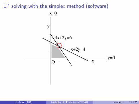
LP solving with the simplex method (software)
O x
y
x+2y=4
3x+2y=6
y=0
x=0
J.Keijsper (TUE) Modelling of LP-problems (2WO09) meeting 1 21 / 70

Special situations: infeasible
O x
y
y=0
x=0
J.Keijsper (TUE) Modelling of LP-problems (2WO09) meeting 1 22 / 70

Special situations: unbounded
O x
y
y=0
x=0
J.Keijsper (TUE) Modelling of LP-problems (2WO09) meeting 1 23 / 70

Special situations: multiple optimal solutions (no Aimmswarning)
O x
y
y=0
x=0
J.Keijsper (TUE) Modelling of LP-problems (2WO09) meeting 1 24 / 70

Special situations: multiple optimal solutions (no Aimmswarning)
O x
y
y=0
x=0
J.Keijsper (TUE) Modelling of LP-problems (2WO09) meeting 1 25 / 70

LP: Sensitivity analysisA parametric curve depicts the sensitivity of an LP model to parametricchange by simply recomputing the optimal solution (or the optimal valueof the objective) for a range of values of the chosen parameter.
parameter
opt.
valueLP
10 90
J.Keijsper (TUE) Modelling of LP-problems (2WO09) meeting 1 26 / 70

Definition Shadowprice
The shadowprice of a constraint in an LP model is the rate of change ofthe optimal value of the objective function from a one unit increase in therighthand side of the constraint (for a small enough increase).
Example
max 2x + 3ys.t. 3x + 2y ≤ 6
x + 2y ≤ 4x ≥ 0
y ≥ 0
J.Keijsper (TUE) Modelling of LP-problems (2WO09) meeting 1 27 / 70

Shadowprice
O x
y
x+2y=4
3x+2y=6
y=0
x=0
2x+3y=3
J.Keijsper (TUE) Modelling of LP-problems (2WO09) meeting 1 28 / 70

Shadowprice
Conclusion: solving the system
x + 2y = 4
3x + 2y = 6
for x and y yields the optimal solution
x = 1
y = 1.5
where the objective function 2x + 3y attains its maximum value 6.5.
J.Keijsper (TUE) Modelling of LP-problems (2WO09) meeting 1 29 / 70

Shadowprice
To compute the shadowprice of the constraint 3x + 2y ≤ 6,change
max 2x + 3ys.t. 3x + 2y ≤ 6
x + 2y ≤ 4x ≥ 0
y ≥ 0
tomax 2x + 3ys.t. 3x + 2y ≤ 7
x + 2y ≤ 4x ≥ 0
y ≥ 0
J.Keijsper (TUE) Modelling of LP-problems (2WO09) meeting 1 30 / 70

Shadowprice
O x
y
x+2y=4
y=0
x=0
2x+3y=3
3x+2y=7
J.Keijsper (TUE) Modelling of LP-problems (2WO09) meeting 1 31 / 70

O x
y
x+2y=4
y=0
x=0
2x+3y=3
3x+2y=7
J.Keijsper (TUE) Modelling of LP-problems (2WO09) meeting 1 32 / 70
Shadowprice
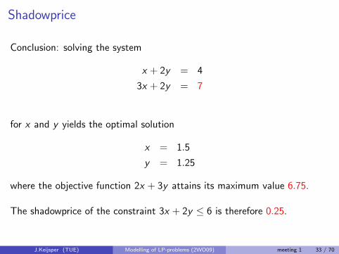
Conclusion: solving the system
x + 2y = 4
3x + 2y = 7
for x and y yields the optimal solution
x = 1.5
y = 1.25
where the objective function 2x + 3y attains its maximum value 6.75.
The shadowprice of the constraint 3x + 2y ≤ 6 is therefore 0.25.
J.Keijsper (TUE) Modelling of LP-problems (2WO09) meeting 1 33 / 70

ShadowpriceSmall enough increase: optimum is intersection of the sameconstraint-lines (no other constraint becomes binding by the increase).
O x
y
x+2y=4
y=0
x=0
2x+3y=3
3x+2y=15
J.Keijsper (TUE) Modelling of LP-problems (2WO09) meeting 1 34 / 70
Shadowprice
Information on the shadowprices of constraints is implicitly available whensolving an LP by the simplex method. In Aimms, simply indicate that youwant this information explicitly.
J.Keijsper (TUE) Modelling of LP-problems (2WO09) meeting 1 35 / 70

Definition Reduced Cost
The reduced cost (or reduced profit) of a variable in an LP model is therate of change of the optimal value of the objective function from a oneunit increase in the bound of the variable that is binding the optimum.(for a small enough increase).
max 2x + 3ys.t. 3x + 2y ≤ 6
x + 2y ≤ 4x ≥ 0
y ≥ 0
J.Keijsper (TUE) Modelling of LP-problems (2WO09) meeting 1 36 / 70
Reduced cost
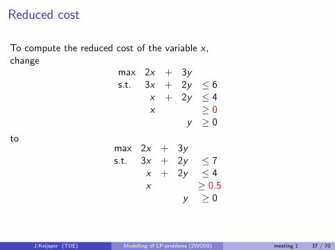
To compute the reduced cost of the variable x ,change
max 2x + 3ys.t. 3x + 2y ≤ 6
x + 2y ≤ 4x ≥ 0
y ≥ 0
tomax 2x + 3ys.t. 3x + 2y ≤ 7
x + 2y ≤ 4x ≥ 0.5
y ≥ 0
J.Keijsper (TUE) Modelling of LP-problems (2WO09) meeting 1 37 / 70

O x
y
x+2y=4
x=0
2x+3y=3
y=0
x=0.5
3x+2y=6
J.Keijsper (TUE) Modelling of LP-problems (2WO09) meeting 1 38 / 70

Reduced cost
Conclusion: Nothing changes.Solving the system
x + 2y = 4
3x + 2y = 6
for x and y yields the optimal solution
x = 1
y = 1.5
where the objective function 2x + 3y attains its maximum value 6.5.
The reduced cost of the variable x is therefore 0.
J.Keijsper (TUE) Modelling of LP-problems (2WO09) meeting 1 39 / 70

Definition MIP
A Mixed Integer Program (MIP) is the task of optimizing (i.e. minimizingor maximizing) a linear function subject to linear inequalities andintegrality constraints on (some of) the variables.
Example
max 2x + 3ys.t. 3x + 2y ≤ 6
x + 2y ≤ 4x ≥ 0
y ≥ 0x integraly integral
Integral variables can model decisions regarding integral numbers andyes/no decisions.
J.Keijsper (TUE) Modelling of LP-problems (2WO09) meeting 1 40 / 70

Example
max 2x + 3ys.t. 3x + 2y ≤ 6
x + 2y ≤ 4x ≥ 0x ≤ 1
y ≥ 0y ≤ 1
x integraly integral
is equivalent tomax 2x + 3ys.t. 3x + 2y ≤ 6
x + 2y ≤ 4x binaryy binary
J.Keijsper (TUE) Modelling of LP-problems (2WO09) meeting 1 41 / 70

LP-relaxationBy deleting all integrality constraints from a MIP, an LP is obtained: itsLP-relaxation.
Example
max 2x + 3ys.t. 3x + 2y ≤ 6
x + 2y ≤ 4x ≥ 0
y ≥ 0x integraly integral
has LP-relaxationmax 2x + 3ys.t. 3x + 2y ≤ 6
x + 2y ≤ 4x ≥ 0
y ≥ 0
J.Keijsper (TUE) Modelling of LP-problems (2WO09) meeting 1 42 / 70

MIP solving by hand: graphical method (2 variables)
O x
y
x+2y=4
3x+2y=6
y=0
x=0
max 2x + 3ys.t. 3x + 2y ≤ 6
x + 2y ≤ 4x ≥ 0
y ≥ 0
J.Keijsper (TUE) Modelling of LP-problems (2WO09) meeting 1 43 / 70
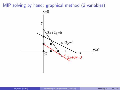
MIP solving by hand: graphical method (2 variables)
O x
y
x+2y=4
3x+2y=6
y=0
x=0
2x+3y=3
J.Keijsper (TUE) Modelling of LP-problems (2WO09) meeting 1 44 / 70
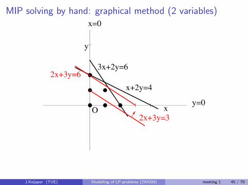
MIP solving by hand: graphical method (2 variables)
O x
y
x+2y=4
3x+2y=6
y=0
x=0
2x+3y=3
2x+3y=6
J.Keijsper (TUE) Modelling of LP-problems (2WO09) meeting 1 45 / 70

MIP solving by hand: graphical method (2 variables)
Conclusion from the picture: optimal solution of this MIP is
x = 0
y = 2
where the objective function 2x + 3y attains its maximum value 6.
J.Keijsper (TUE) Modelling of LP-problems (2WO09) meeting 1 46 / 70

Note: in general, the optimal solution of an MIP is not a corner point ofthe feasible region of the LP-relaxation (and hence can not be obtained asthe solution of a system of constraint-equalities).
O x
y
y=0
x=0
J.Keijsper (TUE) Modelling of LP-problems (2WO09) meeting 1 47 / 70

MIP solving using an LP solver: Branch and Bound
Idea: solve the LP-relaxation. If the optimal solution is not integral,branch: split the feasible region into disjoint parts that both do notcontain this LP-optimum. and solve an LP for each of these parts.
J.Keijsper (TUE) Modelling of LP-problems (2WO09) meeting 1 48 / 70

Branch and Bound
Example
MIP:max 2x + 3ys.t. 3x + 2y ≤ 6
x + 2y ≤ 4x ≥ 0
y ≥ 0x integraly integral
J.Keijsper (TUE) Modelling of LP-problems (2WO09) meeting 1 49 / 70

Branch and Bound
Start by solving the LP-relaxation LP0:
max 2x + 3ys.t. 3x + 2y ≤ 6
x + 2y ≤ 4x ≥ 0
y ≥ 0
LP0 has optimal solution (x , y) = (1, 1.5) and optimal objective value 6.5.
J.Keijsper (TUE) Modelling of LP-problems (2WO09) meeting 1 50 / 70

Branch and Bound Tree
The LP-relaxation can be viewed as the root node of a tree, the branchand bound tree. It corresponds to the entire feasible region.The LP’s for the smaller parts of the feasible region are the other nodes ofthe tree. Every branch from a node corresponds to adding an inequality tothe LP of that node, thereby restricting the feasible region further.
J.Keijsper (TUE) Modelling of LP-problems (2WO09) meeting 1 51 / 70
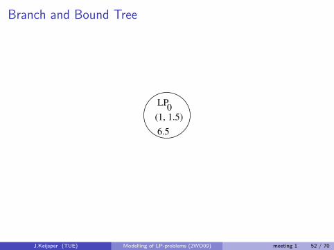
Branch and Bound Tree
LP0
(1, 1.5)
6.5
J.Keijsper (TUE) Modelling of LP-problems (2WO09) meeting 1 52 / 70

Branch and BoundExpand node LP0: branch on variable y :LP1 adds the inequality y ≤ 1 to LP0. LP2 adds y ≥ 2 to LP0.LP1:
max 2x + 3ys.t. 3x + 2y ≤ 6
x + 2y ≤ 4x ≥ 0
y ≥ 0y ≤ 1
LP2:max 2x + 3ys.t. 3x + 2y ≤ 6
x + 2y ≤ 4x ≥ 0
y ≥ 0y ≥ 2
J.Keijsper (TUE) Modelling of LP-problems (2WO09) meeting 1 53 / 70

Branch and Bound
Explore node LP1:max 2x + 3ys.t. 3x + 2y ≤ 6
x + 2y ≤ 4x ≥ 0
y ≥ 0y ≤ 1
optimal solution (x , y) = (113 , 1), objective value 52
3 .
J.Keijsper (TUE) Modelling of LP-problems (2WO09) meeting 1 54 / 70

Branch and Bound
O x
y
x+2y=4
3x+2y=6
y=0
x=0
2x+3y=3
y=1
y=2
J.Keijsper (TUE) Modelling of LP-problems (2WO09) meeting 1 55 / 70

Branch and Bound Tree
LP0
(1, 1.5)
6.5
LP1
LP2
5.67
y>=2y<=1
(1.33, 1)
J.Keijsper (TUE) Modelling of LP-problems (2WO09) meeting 1 56 / 70

Expand node LP1: branch on variable x :LP3 adds the inequality x ≤ 1 to LP1. LP4 adds x ≥ 2 to LP1.LP3:
max 2x + 3ys.t. 3x + 2y ≤ 6
x + 2y ≤ 4x ≥ 0x ≤ 1
y ≥ 0y ≤ 1
LP4:max 2x + 3ys.t. 3x + 2y ≤ 6
x + 2y ≤ 4x ≥ 0x ≥ 2
y ≥ 0y ≤ 1
J.Keijsper (TUE) Modelling of LP-problems (2WO09) meeting 1 57 / 70

Branch and Bound Tree
LP0
(1, 1.5)
6.5
LP1
LP2
5.67
y>=2y<=1
x<=1 x>=2
LP4
LP3
(1.33, 1)
J.Keijsper (TUE) Modelling of LP-problems (2WO09) meeting 1 58 / 70

Branch and Bound
Whenever an integral optimal solution for an LP in one of the nodes isfound, a bound for the best possible MIP objective value is updated. Thetree is pruned in this node.
Explore node LP3:max 2x + 3ys.t. 3x + 2y ≤ 6
x + 2y ≤ 4x ≥ 0x ≤ 1
y ≥ 0y ≤ 1
optimal solution (x , y) = (1, 1) (integer!), objective value 5.New bound: 5. Current best MIP solution: (x , y) = (1, 1).Prune by integrality.
J.Keijsper (TUE) Modelling of LP-problems (2WO09) meeting 1 59 / 70

Branch and Bound
O x
y
x+2y=4
3x+2y=6
y=0
x=0
2x+3y=3
y=1
x=1
J.Keijsper (TUE) Modelling of LP-problems (2WO09) meeting 1 60 / 70

Branch and Bound
The tree can also be pruned at a node if the LP has an optimal solutionwith objective value not better than the current bound.
Explore node LP4:max 2x + 3ys.t. 3x + 2y ≤ 6
x + 2y ≤ 4x ≥ 0x ≥ 2
y ≥ 0y ≤ 1
optimal solution (x , y) = (2, 0) (integer!), objective value 4.Current bound = 5 > 4. No update.Prune by integrality or by bound.
J.Keijsper (TUE) Modelling of LP-problems (2WO09) meeting 1 61 / 70

Branch and Bound
O x
y
x+2y=4
3x+2y=6
y=0
x=0
2x+3y=3
y=1
x=2
J.Keijsper (TUE) Modelling of LP-problems (2WO09) meeting 1 62 / 70

Branch and Bound Tree
LP0
(1, 1.5)
6.5
LP1
LP2
5.67
y>=2y<=1
x<=1 x>=2
LP4
LP3(1,1)
5
(2,0)
4
INTINT
(1.33, 1)
J.Keijsper (TUE) Modelling of LP-problems (2WO09) meeting 1 63 / 70

Explore node LP2:max 2x + 3ys.t. 3x + 2y ≤ 6
x + 2y ≤ 4x ≥ 0
y ≥ 0y ≥ 2
optimal solution (x , y) = (0, 2) (integer!), objective value 6.New bound: 6. Current best MIP solution: (x , y) = (0, 2)Prune by integrality.All nodes are pruned: done.Conclusion: optimal MIP solution: (x , y) = (0, 2), optimal MIP objectivevalue 6.
J.Keijsper (TUE) Modelling of LP-problems (2WO09) meeting 1 64 / 70

Branch and Bound
O x
y
x+2y=4
3x+2y=6
y=0
x=0
2x+3y=3
y=2
J.Keijsper (TUE) Modelling of LP-problems (2WO09) meeting 1 65 / 70

Branch and Bound
LP0
(1, 1.5)
6.5
LP1
LP2
5.67
y>=2y<=1
x<=1 x>=2
(0,2)
6
LP4
LP3(1,1)
5
(2,0)
4
INT
INTINT
(1.33, 1)
J.Keijsper (TUE) Modelling of LP-problems (2WO09) meeting 1 66 / 70
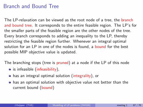
Branch and Bound Tree
The LP-relaxation can be viewed as the root node of a tree, the branchand bound tree. It corresponds to the entire feasible region. The LP’s forthe smaller parts of the feasible region are the other nodes of the tree.Every branch corresponds to adding an inequality to the LP, therebyrestricting the feasible region further. Whenever an integral optimalsolution for an LP in one of the nodes is found, a bound for the bestpossible MIP objective value is updated.
The branching stops (tree is pruned) at a node if the LP of this node
is infeasible (infeasibility),
has an integral optimal solution (integrality), or
has an optimal solution with objective value not better than thecurrent bound (bound)
J.Keijsper (TUE) Modelling of LP-problems (2WO09) meeting 1 67 / 70

Size of the branch and bound tree
For an MIP on n integer variables, each taking a value between 0 and 9,the number of nodes (LPs to solve) can become as large as 10n, soexponential in n.There are no general theorems about how many of those nodes actuallyhave to be explored.
J.Keijsper (TUE) Modelling of LP-problems (2WO09) meeting 1 68 / 70
Binary variables
In a MIP, an integer variable x which is also required to be ≥ 0 and ≤ 1 iscalled a binary variable.
0 ≤ x ≤ 1, x integral
A binary variable models yes/no decisions.
J.Keijsper (TUE) Modelling of LP-problems (2WO09) meeting 1 69 / 70

Sensitivity analysis for MIP
Parametric curves can be constructed for a MIP (but requires solvingmany MIPs so might take too much time for large MIPs).
Shadow prices and reduced costs have no meaning in a MIP. Ignore thevalues Aimms computes for these when solving a MIP!
J.Keijsper (TUE) Modelling of LP-problems (2WO09) meeting 1 70 / 70