MODELLING OF HARD TURNING PROCESS

A thesis submitted in partial fulfilment

Of the requirement for the degree of

Master of Technology

In

Mechanical Engineering

By

Suranjan Mohanty

Department of Mechanical Engineering

National Institute of Technology

Rourkela

May 2014

MODELLING OF HARD TURNING PROCESS

A thesis submitted in partial fulfilment

Of the requirement for the degree of

Master of Technology

In

Mechanical Engineering

By

Suranjan Mohanty

Under Guidance of

Prof. K.P. Maity

Dept. of Mechanical Engg.

Nit, Rourkela

Department of Mechanical Engineering

National Institute of Technology

Rourkela

May 2014

National Institute of technology

Rourkela (India)

CERTIFICATE

This is to certify that thesis entitled, “Modelling of hard turning process’’

submitted by Suranjan Mohanty in partial fulfilment of the requirements for the

award of Master of Technology in Mechanical Engineering with specialization

“Production Engineering” during session 2012-2014 in the Department of

Mechanical Engineering, National Institute of Technology, Rourkela.

It is an authentic work carried out by him under my supervision and guidance.

To the best of our knowledge, the matter embodied in this thesis has not been

submitted to any other University/Institute for award of any Degree or Diploma

Dr. K.P.Maity (Supervisor)

Professor

Dept. of Mechanical Engineering

National Institute of Technology

ACKNOWLEDGEMENT

It gives me immense pleasure to express my deep sense of

gratitude to my supervisor Prof. K.P. Maity for his

invaluable guidance, motivation, constant inspiration and

above all for his ever co-operating attitude that enabled me in

bringing up this thesis in the present form.

I express my sincere gratitude to Mr. Asit Parida, Reserch

scholar for his invaluable guidance during the course of this

work.

I am greatly thankful to all the staff members of the

department and all my well-wishers, class mates and friends

for their inspiration and help.

Suranjan Mohanty

Roll. No:-212ME2290

National Institute of Technology

Rourkela-769008, Odisha, India

CONTENTS

Item Page.no List of tables i

List of figures ii

Abstract iii

CHAPTER-1 Introduction

1.1. Advantages(Benefits) of hard machining 1

1.2. Limitations (Draw backs) of hard machining 1

1.3. Features in which hard machining is different

from conventional machining 2

1.4. Factors distinguishing hard machining 3

1.5. Hard turning 4

CHAPTER-2 Literature review 6

CHAPTER-3 Theoretical study 11

3.1. Surface roughness 11

3.1.1. Terms used in surface finish 12

3.1.2. Different parameters used in measuring

Surface roughness 13

3.1.3. Methods of measuring surface roughness 14

3.2. Tool wear in turning 15

3.3. Cutting tool materials used in case of hard

Machining. 17

3.4. Taguchi method 20

CHAPTER-4 Experimental Details 22

4.1. Work material 22

4.2. Cutting inserts 23

4.3. Tool holder 25

4.4. Lathe machine used for experiment 26

4.5. Surface roughness tester used for experiment 27

4.6. Micrometre used for experiment 28

4.7. Experimental procedure 29

4.8. Final experimental table 31

4.9. Chip collected during experiment 33

4.10. Photographs of tool wear 36

CHAPTER-5 Results and discussion 39

5.1. Main effect plots for surface roughness 39

5.2. Main effect plots for power consumption 40

5.3. Main effect plots for chip reduction co-efficient 41

5.4 Main effect plots for tool wear 42

5.5. ANOVA and response table for surface roughness 43

5.6 ANOVA and response table for power consumption 45

5.7. ANOVA and response table for chip reduction

Co-efficient. 46

5.8. ANOVA and response table for tool wear. 47

CHAPTER-6 Conclusion and future work 49

6.1. Conclusion 49

6.2. Future work 50

CHAPTER-7 Bibilography 51

List of tables

Table No. Item Page No.

4.1 Chemical composition of Cr-Mo alloy 23

4.2 Levels of input parameters 30

4.3. Table for calculation of power, chip thickness,

and chip reduction co-efficient. 30

4.4 Final experimental table containing S.R, power,

Chip reduction co-efficient and tool wear. 31

5.1. ANOVA for surface roughness. 44

5.2. Response table for surface roughness. 44

5.3. ANOVA for power consumption. 45

5.4. Response table for power consumption. 46

5.5. ANOVA table for chip reduction co-efficient. 47

5.6. Response table for chip reduction co-efficient. 47

5.7. ANOVA table for tool wear. 48

5.8 Response table for tool wear. 48

i

LIST OF FIGURES

Figure.no. Item Page.no

3.1. Development of flank wear 17

4.1. Work piece material(Cr-Mo round bar) 22

4.2. Inserts used in the experiment 24

4.3. Tool holder(PSBNR 2525 M12) 25

4.4. Lathe machine with work piece used in experiment 26

4.5. Taylor-Hobson(Sutronic 3+) 27

4.6. Micrometer 28

4.7. Chips collected during experiment 33

4.8. Photographs of tool wear 36

5.1. Main effect plots of surface roughness 39

5.2. Main effect plots of power consumption 41

5.3. Main effect plots of chip reduction co-efficient 42

5.4 Main effect plots of tool wear 43

ii

Abstract In the present work, the workpiece material taken is chrome-moly alloy steel. This is a hard

material having hardness 48 HRC. This alloy steel bears high temperature and high pressure

and its tensile strength is high. It is very resistive to corrosion and temperature. For these

useful properties it is used in power generation industry and petrochemical industry. Also it is

used to make pressure vessels. For machining of workpiece the insert chosen is Tic coated

carbide insert. Three factors speed, feed and depth of cut were taken at three levels low,

medium and high. By the L27 orthogonal design twenty seven runs of experiments were

performed. For each run of experiment the time of cut was 2 minutes. The output responses

measured were surface roughness, power consumption, chip reduction co-efficient and tool

wear (flank wear). All the output responses were analyzed by SN ratio, analysis of variance,

and response table. The criteria chosen here is smaller the better and the method applied is

Taguchi method.

iii

1 | P a g e

CHAPTER-1

INTRODUCTION

Hard machining means machining of parts whose hardness is more than 45HRC but actual hard

machining process involves hardness of 58HRC to 68HRC.The work piece materials used in

hard machining are hardened alloy steel , tool steels , case – hardened steels , nitride irons ,

hard – chrome – coated steels and heat – treated powder metallurgical parts[16].

1.1.Advantages (Benefits) of hard machining:-

1. Complex part contours can be easily machined by this process.

2. Component types can be quickly changed over in this process.

3. In one set – up, many operations can be completed.

4. Metal removal rate is very high.

5. The CNC Lathe which is used for soft turning process can be used for this process.

6. Investment in machine tool is very low.

7. Metal chips produced in the process are environmentally friendly.

8. No coolant is required in many cases.

9. Tool inventory required is small.

1.2.Limitations (Draw backs) of hard machining:-

1. The cost of tooling in case of hard machining is higher than grinding.

2. For hard turning the length to diameter (L/D) ratio should be small. For unsupported work

pieces it should not be more than 4:1 because long thin parts will induce chatter due to high

cutting pressure.

2 | P a g e

3. For hard machining to be successful, the machine used must be rigid. The degree of hard

turning accuracy is known from degree of machine rigidity. If we want to maximise the

machine rigidity than we have to minimise overhangs, tool extensions and to eliminate shims

and spacers.

4. The main challenge in hard machining is whether or not to use coolants, in some cases where

there are interrupted cuts such as gears dry machining is good. Due to shock produced by

thermal effect the insert will feel exiting and entering cut and insert will break. In case of

continuous cut due to high tool tip temperature softens the area which are machined previously

and decreases the value of hardness due to which material is easily cut. But due to dry

machining part thermal distortion, handling and in process gauging is difficult so if coolant

will be used then water based coolants should be used[16].

5. Surface finish decreases with increase of tool wear in the range of tool life.

6. In hard machining, a very thin layer of material which is harder than inner material is formed

which is known as white layer. With tool wear increase its thickness increases. White layer is

commonly formed on bearing steel and makes problem for bearing races which receive high

contact stresses. The white layer causes bearing failure.

1.3. Features in which hard machining is different from conventional machining:-

1. When work material gets fractured chip in the form of saw tooth is formed. Within the range

of shear strain crack is formed at the free surface of the workpiece.

2. Because of adiabatic shear segmental chips are formed in materials which are difficult to

machine and its cross section is similar to saw-toothed chip formed in hard machining but these

two chips are not same because they are produced due to different mechanisms.

3 | P a g e

3.The shear angle in case of hard machining is very small and increases with increase of

hardness of work material and do not depend upon tool rake angle but the shear angle in case

of traditional machining is large.

4. Radial (thrust) component of the cutting force is greater than tangential (power) component

cutting force in case of hard machining. The difference between these two forces increases with

increase of flank wear.

5. The tangential (power) component and radial (thrust) component depend upon the tool rake

angle. At zero rake angle the components do not increase with hardness of material. At tool

rake angle -20 degree, these components reduce with hardness of work material.

6. The chip compression ratio is equal to two in case of hard machining.

7. The radial component and tangential component depend upon flank wear differently. When

flank wear increases from zero to 0.2mm the radial component increases four fold.

1.4.Factors distinguishing hard machining:-

To distinguish between hard machining conventional machining differences in energy balance

should be analysed. The formula for balance of energy in metal cutting is given by Pc = Fc.V

=Ppd +Pfr +Pjf +Pch

Where Fc = power(tangential) component of the cutting force.

V = cutting speed

Ppd = power consumed due to plastic deformation

Pfr = power used on tool chip interface

Pjf = power used on tool work piece interface

Pch = power used due to formation of new surfaces

4 | P a g e

The difference in the energy balance in conventional and hard machining of AISI steel 52100

the following conclusions are made[16].

1. In hard machining power spent on tool work piece surface is greatest but in conventional

machining it is opposite.

2. Much power is spent in formation of new surfaces in hard machining.

3. Also power spent in the plastic deformation of layer being removed is much.

1.5.Hard turning:-

Hard turning is a process which eliminates the requirements of grinding operation. A proper

hard turning process gives surface finish Ra 0.4 to 0.8 micrometre, roundness about 2-5

micrometre and diameter tolerance +/-3-7micrometre. Hard turning can be performed by that

machine which soft turning is done. The starting point of hard turning is the material hardness

47 HRC but regularly hard turning is done on the material having hardness 60HRC and higher.

The materials required for hard turning are tool steel, case-hardened steel, bearing steel,

Inconel, Hastealloy, stellite and other exotic materials are also falling in the category of hard

turning. The length to diameter ratio(L/D) ratio for unsupported work piece should not be more

than 4:1 because though tailstock support is there for long thin parts chatter would be induced

due to high cutting pressure. The degree of hard turning accuracy is measured by degree of

machine rigidity. The system rigidity is more required for hard turning than machine rigidity.

If rigidity of system is to be maximised then overhangs, extensions of tools, extensions of parts

should be minimised and shims and spacers should eliminated. The purpose is to keep

everything as close to turret or spindle as possible. The main challenge in hard turningis

whether coolant will be used or not. In maximum cases hard turning will be performed dry.

When hard turning will be performed without coolant, part will be hot. Due to this, it will be

difficult for process gauging. To cool down the machined part coolant is used through the tool

5 | P a g e

with high pressure. Additional problems are created due to flying cherry red chips. Mainly

water-based and low concentration coolants are used in hard turning. In hard turning maximum

heat is transferred to chip so if chip will be examined during and after cut then whether the

process is well turned or not will be known. The chips should be glowing orange and flow like

ribbon during continuous cut. If we will crunch the cooled chip and it will disintegrate then it

shows that proper amount of heat is produced[16].

6 | P a g e

CHAPTER-2

LITERATURE REVIEW

Dilbag singh and P. Venkateswara Rao [1] investigated how surface roughness in bearing

steel(AISI 52100) is effected by cutting condition and tool geometry. In this investigation

mixed ceramic inserts which are made from Aluminium oxide and Titanium

carbonitride(SNGA) which have different nose radius and different effective rake angle are

used. In this study they concluded that S.R is effected by feed significantly followed by nose

radius and cutting velocity. S.R. is effected very less by effective rake angle but interaction

effect of nose radius and effective rake angle is significant. RSM is used to develop

mathematical model.

Tugrul O zel et all [2] have investigated how surface roughness and resultant force in hard

turning of AISI H13 steel is effected by cutting edge geometry, hardness of workpiece, feed

and cutting speed. In this investigation four factor two level fractional factorial experiments

are used and ANOVA is applied. Hardness of workpiece, geometry of edge, feed and cutting

speed are the four factors. In hard turning experiment cutting force, feed force, thurst force and

surface roughness were measured. From the study the significant factors on surface roughness

are found to be hardness of workpiece, geometry of cutting edge, feed and cutting speed. Lower

workpiece hardness and honed edge geometry produce better S.R. Geometry of cutting edge,

hardness of workpiece, cutting speed affect force components.

B. Fnides et all conducted the experiment to determine the statistical model of surface

roughness in hard turning of high alloyed steel X38CrMo5-1. This steel is hardened to 50HRC

and is machined by mixed ceramic tool (insert cc650 of chemical composition 70% Al2O3 +

30% Tic) free from Tungsten on Cr-Mo-V basis, intensive to temperature changes and high

wear resistance. By 33 full factorial design total 27 experiments were carried out. The levels

7 | P a g e

low, medium, and high of the parameters are set. Mathematical models are deduced by multiple

regression method in order to express the influence of each cutting regime element on surface

roughness. Finally the result concludes that feed rate is the main factor influencing surface

roughness followed by cutting speed. Depth of cut has not any important effect on surface

roughness.

Dr. G. Hrinath Gowd et all [4] studied on Fx, Fy, Fz and S.R. and developed second order

polynomial model for them. Mainly the problems in turning are due to cutting parameters ( Fx,

Fy, Fz and S.R.). Experiments were performed and it is concluded that cutting force, feed force

, thurst force and surface roughnessare significantly affected by speed, feed and depth of cut.

Prediction of mathematical models fo estimation of Fx, Fy, Fz and S.R , RSM is used.

K. Adarsh kumar et all [5] investigated how surface finish of EN-8 is affected by spindle speed,

feed, depth of cut. Experimental measurements were determined multiple regression analysis

and ANOVA. Cemented carbide inserts are used to predict surface roughness by multiple

regression analysis. The purpose is to form arelation between cutting speed, feed and depth of

cut to optimise S.R. using multiple regression analysis.

S.B. Salvi et all [6] studied on hard turning of 20MnCr5 steel. The purpose of this study is to

analyse optimum cutting conditions to get lowest surface roughness in turning of 20MnCr5

steel. Taguchi method is applied in this process. Orthogonal array, signal to noise ratio and

analysis of variance are applied to investigate the cutting characteristics. From the experiment

it is concluded that feed rate has the significant role to produce lower surface roughness

followed by cutting speed. In this experiment the cutting insert used is ceramic based

TNGA160404.

F.Puh et all [7] used Taguchi design and optimised the process parameters for hard turning of

AISI 4142 and in this experiment he used PCBN tool. L9 orthogonal array having three level

8 | P a g e

and four factor, SN ratio and ANOVA are used for this to study cutting parameters(speed, feed,

depth of cut) with consideration of S.R. Multiple regression analysis was used to find first order

linear and second order prediction model for surface roughness and independent variables.

Ali Riza Motorcu [8] investigated how S.R. in turning of AISI 8660 is affected by cutting

speed, feed, depth of cut and tool nose radius using P.V.D. coated ceramic cutting tool. He

analysed the process by orthogonal design, SN ratio, ANOVA and found that feed rate is the

effective parameter followed by depth of cut and nose radius. Cutting speed is not significant.

Due to surface hardening effect the interaction of feed and d.o.c was found to be significant.

R. Ramanujan et all [9] presented a new methodology for the optimisation of the machining

parameters on turning Al-15% SiCp metal matrix composites. Desirability function analysis is

applied optimise the machining parameters. Experimental design for the experiment is L27.

Multiple performance considerations namely surface roughness and power consumption is

applied for optimisation of the machining parameters such as cutting speed, feed rate, depth of

cut. Composite desirability value is used to find optimum machining parameters.

A.D. bagawade et all [10] evaluated the area ratio of chip. He also evaluated S.R. in hard

turning of AISI52100(EN-31) steel. The hardness of steel was about 48-50 HRC and this was

machined by PCBN tool. The effect of speed, feed, depth of cut on chip area ratio and S.R were

found.

S. Delijaicov et all [11] studied the effect of vibrations of cutting in hard turning process of

AISI 1045. The specimen is first tempered and then quenched upto 53 HRC. Piezoelectric

dynamometer as well as acquision data system is used for measurement. Excellent correlation

is obtained between model and results and this showed frequency amplitude increases

reliability of model by 5%.

9 | P a g e

P.V.S Suresh et all [12] used RSM to study surface roughness prediction model for turning of

mild steel. CNMG cutting tools are used for experiment. A second order mathematical model

is developed for surface roughness using RSM.

B. Sidda reddy et all [13] developed surface roughness model for machining of aluminium

alloys , using adaptive neuro-fuzzy interference system(ANFIS). CNC machine is used for

experimentation with carbide cutting tool for machining Aluminium alloys for a wide range of

machining conditions. The ANFIS model has been developed in terms of machining parameters

to predict the surface roughness using train data. To validate the model the experimental

validation runs were conducted. Percentage deviation and average percentage deviation has

been used to judge accuracy and ability of model. Same data were modelled by RSM and the

ANFIS results are compared with RSM results and it is concluded that ANFIS are superior to

RSM results.

Tugrul o Zel, Yigit Karpat [14] used neural network modelling for prediction of surface

roughness and tool flank wear over machining time for varity of cutting conditions in finish

hard turning. For training neural network model the data from measured surface roughness and

tool flank wear of AISI H-13 steel were used. For other cutting conditions trained neural

network models were used in predicting surface roughness and tool flank wear. Comparison

between neural network model and regression model is done and better prediction is obtained

from predictive neural network model for surface roughness and tool wear within the training

range. When feed rate is decreased surface roughness becomes better but tool wear becomes

faster. When cutting speed is increased tool wear is increased but surface roughness becomes

better. When work piece hardness is increased surface roughness becomes better but tool wear

becomes larger. Finally it is concluded that CBN inserts with honed edge geometry performed

better surface roughness and tool wear development.

10 | P a g e

Y.Kevin Chou, Hui Song [15] employed a mechanistic model to estimate the chip formation

forces. Assuming linear growth of plastic zone on the wear land and quadratic decay of stresses

in the wear land forces are modelled. Increasing feed rate and cutting speed adversely affect

maximum machined surface temperature in new cutting tool but increasing depth of cut

favourably affect the maximum machined surface temperature.

11 | P a g e

CHAPTER-3

THEORITICAL STUDY

3.1 Surface roughness:-

Due to the increased knowledge and constant improvement of the surface textures gives

the present machine age a great advancement. Due to the demand of greater strength and

bearing loads smoother and harder surfaces are needed. The surface texture has direct contact

with the functioning of machine parts, load carrying capacity, tool life, fatigue life, bearing

corrosion and wear qualities. Failure due to fatigue always occurs at the sharp corners because

of stress concentration at that place. Sharp corner is the place where any surface irregularity

starts and that part fails earlier. Surface irregularity at non-working surface also matters for

failure. Different requirements demand different types of surfaces so measurement of surface

texture quantitatively is essential. The imperfections on the surface are in the form of

succession of hills and valleys varying both in height and spacing. Any material being

machined by chip removal process cannot be finished perfectly due to some departures from

ideal conditions. Due to conditions not being ideal the surface being produced will have some

irregularities and these irregularities can be classified into four categories given as

follows[17]:-

a) First order:- This type of irregularities are arising due to inaccuracies in the machine tool

itself for example lack of straightness of guide ways on which tool post is moving. Irregularities

produced due to deformation of work under the action of cutting forces and the weight of the

material are also included in this category.

b) Second order:- This order of irregularities are caused due to vibration of any kind such as

chatter marks.

12 | P a g e

c) Third order:- If the machine is perfect and completely free of vibrations still some

irregularities are caused by machining due to characteristics of the process. For example feed

mark of cutting tool.

d) Fourth order:- This type of irregularities are arised due to rupture of the material during the

separation of the chip.

Further these irregularities of four orders can be grouped under two groups. First group includes

irregularities of considerable wave-length of the periodic character resulting from mechanical

disturbances in the generating set up. These errors are termed as macro-geometrical errors and

include irregularities of first and second order. These errors are also referred to as waviness or

secondary texture. Second group includes irregularities of small wavelength caused by the

direct action of the cutting element on the material or by some other disturbances such as

friction, wear or corrosion. Errors in this group are referred to as roughness or waviness.

3.1.1Terms used in surface finish:-

Roughness:- This is produced due to irregular structures in the surface roughnesswhich is

resulted from the inherent action of production process.

Waviness:- This is produced due to deflection in work piece or machine vibrations produced

in machine.

Flaws:- The irregularities which are produced at one place or infrequently in widely varying

intervals in a surface are called flaws.

Centre line:-The line about which roughness is measured.

Traversing length: - It is the length of the profile necessary for the evaluation of the surface

roughness parameters. The traversing length includes one or more sampling lengths.

13 | P a g e

Sampling length:-It is the length of profile necessary for the evaluation of the irregularities to

be taken into account also known as cut off length.

Mean line of the profile:- It is the line having the form of the geometrical profile and dividing

the effective profile so that within the sampling length the sum of squares of the distances

between effective points and the mean line is minimum.

Centre line of the profile:-It is the line parallel to the general direction of the profile for which

the areas embraced by the profile above and below the line are equal.

Spacing of the irregularities:- It is the mean distance between the more prominent irregularties

of the effective profile, within the sampling length.

3.1.2 Different parameters used in measuring surface roughness:-

Arithmetic average roughness:- Ra=1/𝐿 ∫ 𝑚𝑜𝑑(ℎ)𝑑𝑥𝐿

0 over 2-20 consecutive sampling

lengths.

Average peak-to-valley height(Rz):-This is the average of single peak-to-valley heights from

five adjoining sampling lengths.

Depth of surface smoothness:-Rp=1/L∫ (𝐻𝑚𝑎𝑥 − 𝐻)𝑑𝑥𝐿

0

Levelling depth(Ru):- Distance between mean line and a parallel line through highest peak.

Mean depth(Rm):-Distance between mean line and a parallel line through the deepest valley.

Maximum peak-to-valley height(Rmax):-Largest single peak-to-valley heights in five adjoining

sampling lengths.

Root mean square roughness:-Rq= √1/𝐿 ∫ ℎ2𝐿

0𝑑𝑥

14 | P a g e

3.1.3Methods of measuring surface roughness:-

There are two methods of measuring the finish of machined part[17]. They are :-

(i) Surface inspection by comparison methods

(ii) Direct instrument measurements

(i) Surface inspection by comparison:-

In comparative methods the surface texture is assessed by observation of the surface. But these

methods are not reliable as they can be misleading if comparison is not made with surfaces

produced by same techniques. The various methods available under comparison method are:-

(i) Torch inspection

(ii) Visual inspection

(iii) Scratch inspection

(iv) Microscopic inspection

(v) Surface photographs

(vi) Micro-Interferometer

(vii) Wallace surface dynamometer

(viii) Reflected light intensity

(ii)Direct instrument measurement:-.

Stylus probe instruments are as follows:- Surface finish of any surface can be measured by

this method. In this type measurement electrical principles are used and they are stylus probe

type instrument. There are two types of these electrical instruments. Carrier modulating

principle is the first type of operation. The movement of the stylus exploring the surface are

caused to high frequency carrier current. Second type works onvoltage generating principle.

(i) Profilometer

15 | P a g e

(ii) The Tomlinson surface meter

(iii) The Taylor-Hobson Talysurf

(iv) Stylus

Out of the above four only Taylor-Hobson Talysurf is used in our experiment this to calculate

surface roughness.

3.2.Tool wear in turning:-

A constant cutting force is acting in turning operation and turning is a continuous process. A

high temperature is produced at the tool/chip interface because of constant heat derived from

shear deformation energy and friction. The principal wear factor in turning is high temperature

at the tool rake face. The temperature is around 600 degree for austenitic steels, super alloys or

titanium alloys. Tool wear mechanisms in turning are basically four types in turning[16]. They

are as follows:-

(i) Crater wear

(ii) Notch wear

(iii) Flank wear

(iv) Adhesion

Crater wear: It is a chemical or metallurgical wear. Crater wear is produced because

small particles of the tool rake surface diffuse or adhere on fresh chip. Scar like shape

is produced on the rake face due to mechanical friction and it is parallel to the major

cutting edge. In turning of titanium alloys and low thermal conductivity materials crater

wear is produced.

16 | P a g e

Notch wear: It is a combination of flank wear and rake face wear which occurs just in

the point where major cutting edge intersects the work surface. This type of wear is

produced in those materials which have a tendency to surface hardening due to

mechanical loads. When tool passes rub the fresh machined surface increases hardness

of the outer layer. In turning of austenitic stainless steels and nickel-based alloys notch

wear is produced.

Flank wear: This type of wear is produced on the flank face of the tool. Wear land formation

is not uniform along major and minor cutting edge of the tool. This type of wear is produced

in case of hard materials because there is not any chemical affinity between tool and

material. The wear mechanism is due to abrasion in this case.

Adhesion: Welding occurs between the fresh surface of the chip and tool rake face

because high pressure and temperature. If materials have metallurgical affinity the there

will be better welding and that will produce a thick adhesion layer and tearing of the

softer rubbing surface at high wear rate. In Aluminium alloys this type of wear is

produced in dry conditions. In hard machining this type of wear is not produced.

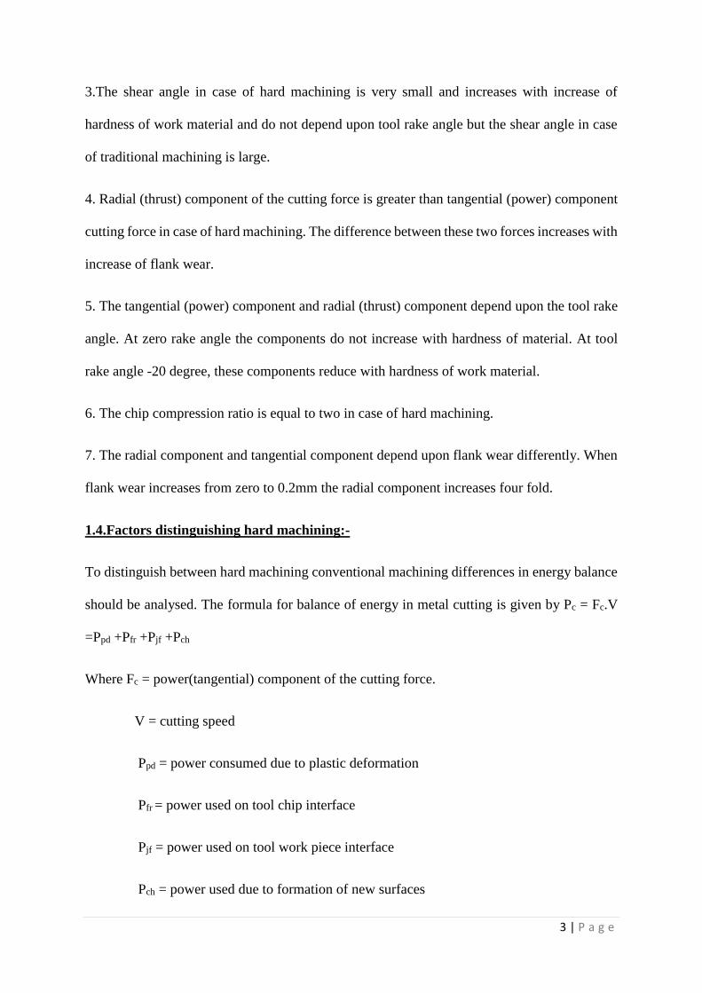
Wear curve: The following curve shows mean flank wear(VB) along time for various cutting

speeds. This wear curve is divided into three regions as given below in fig-3.5.

Initial wear region: In this region the sharp new edge worn rapidly. The wear size VB

= 0.05-0.1 mm in this region.

Steady wear region: In this region wear rate is constant and increases slowly. In this

zone VB=0.05-0.6 mm onwords.

17 | P a g e

Severe wear region: In this region tool wears in very high rate. When this zone is

reached anew tool must be used in place of worn tool or sharpening must be done before

tool breakage.

Fig-3.1: Development of flank wear with respect to time

3.3 Cutting tool materials used in case of hard machining:-

During hard machining high temperatures are produced and big mechanical load is there due

to speed so cutting tools must withstand these two things. In some cases the temperature in the

tool/chip interface reaches around 700 degree centigrade[16]. Severe friction is produced

between tool and chip as well as tool and new machined surface. Keeping in mind the above

things the cutting tool materials should have the following properties:

Cutting tool substrate material must be chemically and physically stable at high

temperatures.

Material hardness must withstand high temperatures produced at the chip/tool interface.

For abrasion and adhesion mechanisms tool material should have a low wear ratio.

18 | P a g e

To perform interrupted and intermittent cutting tool material must have enough

toughness to avoid fracture.

Starting from the lowest hardness to the highest hardness the tool materials can be classified as

follows:-

High speed steel (H.S.S.)

Sintered carbide

Ceramics

Extra hard materials

High speed steel: These are of high content carbon steels with a high proportion of alloying

elements such as tungsten, molybdenum, chromium, vanadium and cobalt. Hardness is about

75 HRC. The T series includes tungsten, the M series molybdenum. Vanadium produces the

hardest carbides and produces super high speed steels. HSS can withstand temperature upto

500 degree centigrade. The HSS produced by power metallurgy process(HSS-PM) possesses a

higher content alloying elements and unique properties like higher toughness, higher wear

resistance, higher hardness, higher hot hardness.

Sintered carbide: Mixing tungsten carbide micro grains with cobalt at high temperature and

pressure sintered carbide tools are produced. These are also known as cemented carbide tools.

Tantalum, Titanium, Vanadium carbides are also mixed in small amount. Sintered carbides are

described by two main factors. One is the ratio of tungsten carbide and cobalt. Cobalt ranges

from 6 to 12% and it acts as binder. Melting point of Cobalt is 1493 degree centigrade. Cobalt

forms a soluble phase with tungsten carbide grains at 1275 degree centigrade and helps to

reduce porosity. Second is the micro grain size. Micro grain size is smaller than 1 micrometre

and submicrograin are smaller than half micron. The hardness of sintered carbide increases

with the reduction in binder content and tungsten carbide grain size. Hardness of sintered

19 | P a g e

carbide ranges from 600HV to 1200HV. Sintered carbides are manufactured in two forms,

integral tools and inserts. Sintered carbides are classified into six groups M, P, K, N, S, H. Each

scale includes a numerical scale for it. In USA C-x scale is used. M, grade includes the sintered

carbides suitable for stainless steel machining. P, includes sintered carbides for low and

medium carbon steels and light alloyed steels. K, includes sintered carbides for cast irons and

alloyed steels. N, is used for Aluminium alloys, S, for heat resistant alloys and H, for tempered

and hardened steels. For each of the above grades the two digit number 01 to 40 is used, except

P, for which 01 to 50 is used. Lower number indicates harder grades and higher number

indicates tougher grades. In USA C-1 to C-4 are general grades for cast iron, C-5 to C-8 are

for steel alloys, C-9 to C-11 for high wear applications, C-12 to C-14 for impact cases. The two

basic groups of carbides used for machining are tungsten carbide and Titanium carbide[16].

a) Tungsten carbide: WC particles are bonded together with cobalt matrix to give tungsten

carbide composite. By powder metallurgy technique WC particles are bonded together

with cobalt in a mixer resulting in cobalt matrix surrounding WC particles and by this

process tungsten carbide tools are manufactured. WC is frequently compounded with

Titanium and Niobium to impart special properties to the carbide. Steels, Cast irons and

abrasive non-ferrous materials are cut by Tungsten carbide tools.

b) Titanium carbide: Tic has higher wear resistance than WC but it is not as tough as WC.

Nickel-molybdenum alloy is used as matrix. Steels and cast irons can be machined by

TIC.

Ceramics: Ceramics can be used for machining the metals at high cutting speeds and in dry

machining conditions because these are very hard and refractory materials which can withstand

up to 1500 degree centigrade without chemical decomposition. Ceramic powders are used to

mould ceramic materials at pressures 25MPa. Sintering of ceramic materials are done at 1700

degree centigrade. Ceramic tools may be of three types for example alumina tools (Al2O3),

20 | P a g e

Silicon nitride (Si3N4) and sialon which is combination of Si, Al, O and N. Alumina tools

contain mixture of titanium, magnesium, chromium, or zirconium oxides distributed into

alumna matrix homogenously. Due to this toughness gets improved. Silicon nitride ceramics

have a higher resistance to thermal shock and a higher toughness. Ceramics have a needle like

structure embedded in grain boundary which increases fracture toughness. These are applied

for roughing cast iron under heavily interrupted cuts. Ceramic tools must be kept hot

throughout the operation and shocks on tool edges at tool entrances exits from the work piece

must be avoided.

Extra-hard materials: Extra-hard materials include PCD and PCBN. PCD is used for machining

abrasive non-ferrous metals, plastics and composites. PCBN is used for machining of hardened

tool steels and cast irons.

3.4.Taguchi method:-

The methodology applied in this study is Taguchi method. It is a combination of methodologies

by which inherent variability of materials and manufacturing processes has been taken into

consideration during design. Controlled and noise both factors are considered in this design.

Taguchi design is similar to design of experiment but it conducts the orthogonal experimental

combinations which makes the method more effective than fractional factorial design. Taguchi

method uses special design of orthogonal arrays to study the entire patameter space with small

no of experiments. Taguchi uses the loss function for the measurement of the performance

characteristics deviating from the desired value. The value of loss function is converted to S/N

ratio. There are three types of S/N ratios e.g lower-the-better, Higher-the-better, Nominal-is-

best. The formula for three types of S/N ratio is given below.

21 | P a g e

Nominal-is-the-best:S/NT=10log(�̅�

𝑠𝑦2)

Larger-is-the-better (maximise):S/NL=-10log(1

𝑛∑

1

𝑦𝑖2

𝑛𝑖=1 )

Smaller-is-the-better (minimise):S/Ns=-10log(1

𝑛∑ 𝑦𝑖

2𝑛𝑖=1 )

Where �̅� is the average of observed data and 𝑠𝑦2 is the variance

of y, n is the no. of observations and y is the observed data. S/N ratio is always expressed in

decibel. If the objective is to reduce the variability around a specific target then S/NT is used.

If the system is optimized when response is as large as possible S/NL is used. If the system is

optimized when the response is optimized as small as possible S/Ns is used. The goal of this

research is to produce minimum surface roughness, minimum power consumption, minimum

chip reduction co-efficient, and minimum tool wear in turning operation. The larger value of

S/N ratio means the better performance characteristics so the optimal level of the process

parameters is the level with the highest S/N ratio. A statistical analysis of variance is

performed to see statistically significant process parameters.

In this paper three factors speed, feed and depth of cut are taken as the control parameters.

Each factor has three levels low, medium and high so L27 orthogonal array has been choosen

which has 27 rows corresponding to the number of parameter combinations having 26

degrees of freedom.

22 | P a g e

CHAPTER-4

EXPERIMENTAL DETAILS

4.1. Work piece material: The work piece is chrome-moly alloy which is prepared at cast profile

private limited, Kalunga. Its length is 600 mm and diameter is 50 mm. It is heat treated to make

its hardness upto 48 HRCThe photograph of work piece material and chemical composition of

the CR-MO alloy is given below in fig-4.1:

Fig-4.1: Work piece material(Cr-Mo round bar)

Dimension of Cr-Mo alloy:

Length of bar = 600 mm

Diameter of bar = 50 mm

Hardness of material =48 HRC

23 | P a g e

Chemical composition of Cr-Mo alloy(Table-4.1)

Carbon Mn Cr Mo

0.15 max 0.3-0.6 4.0-6.0 0.44-0.65

4.2.Cutting inserts:-

Cutting inserts used in this experiment are four in number. Each insert has eight edges so for

27 experiment all eight edges of first three are used and three edges of last insert is used. The

specification of insert is SNMG 120408. The inserts are Tic coated carbide inserts. The

photographs of all inserts used in experiment, their specification and geometry are given below

in fig4.2(a), (b), (c), (d):

Insert-1 Insert-2

[a] [b]

24 | P a g e

Insert-3 Insert-4

[c] [d]

Fig-4.2

Specification of inserts:-

SNMG120408

S:-Insert shape (square)

N:-Clearance angle (0 degree)

M:-Tolerances

G:-Form of top surface

12 mm:-Cutting edge length

04 mm:-Insert thickness

08 mm:-Corner radius

Geometry of inserts:-

Inclination angle=-6 degree

Orthogonal rake angle=-6 degree

25 | P a g e

Orthogonal clearance angle= 6 degree

Auxiliary cutting edge angle= 15 degree

Principal cutting edge angle= 75 degree

Nose radius = 0.8 mm

4.3.Tool holder: - The tool holder used for the experiment is PSBNR2525M12. Its

photograph and specification is given below in fig4.3.

Fig-4.3:Tool holder (PSBNR2525M12)

Specification of tool holder:-

P:-Clamping method (Retained via bore)

S:-Insert shape (square)

B:-Style (75 degree)

N:-Clearance angle (0 degree)

R:-Cutting direction (right handed)

25 mm:-Shank height

26 | P a g e

25 mm:-Shank width

M:-Tool length150 mm

12 mm:-Cutting edge length

4.4.Lathe machine used for experiment:-

The type of machine used for hard turning Cr-Mo alloy is conventional lathe machine with

high rigidity. Cutting tests were carried out under dry cutting environment. Dry machining has

been considered as the machining of the future due to concern regarding the safety of the

environment. The experimental set-up is given in fig-4.4.

Fig-4.4:Lathe machine with work piece

27 | P a g e

4.5.Surface roughness tester used in experiment:-

Fig-4.5:Taylor-Hobson (sutronic 3+)

Specification:-

Traverse speed: 1 mm/second

Measurement unit: Metric/Inch

Cut-off values: 0.25 mm, 0.80 mm, 2.5 mm (0.01 in, 0.03 in, 0.1 in)

Parameters: Ra, Rq, Rz(DIN), Ry and Sm

Calculation time: Less than reversal time or 2 second whichever is longer

28 | P a g e

4.6.Micrometre used to calculate chip thickness:- The micrometre used to calculate chip

thickness is given below in fig-4.6 with its specification.

Fig-4.6: Micrometre

Specification:

Least count: 0.01 mm

Range: 0-25 mm

29 | P a g e

4.7.Experimental procedure:

The rough work piece of chrome-moly alloy bought from cast profile Ltd, kalunga is first

turned to clear the rough skin using uncoated carbide insert. The final diameter of the work

piece is made 50 mm. The two ends of the work piece are faced and centring is done using

carbide centre drill. The final length of the work piece was made 600 mm. The purpose of this

experiment is to find the effect of speed, feed and depth of cut on output responses like surface

roughness, power consumption, chip reduction coefficient and tool wear. The levels of speed,

feed and depth of cut are three each which is given in table-4.2. Total 27 experiments were

done according to L27 orthogonal array. The work piece was held rigidly on the lathe and for

each set of the data work piece is turned for 2 minutes so 27 cuts were made on the workpiece

which is shown in Fig-4.1. The surface roughness component (Ra) was measured using

Taylor/Hobson (sutronic 3+) for 27 cuts. The power consumed in machining was measured by

wattmeter connected to the Lathe machine. The wattmeter gave the reading of voltage (V),

current (I) and power factor (cosϕ) for each of the runs of the experiment. The power

consumption can be given by formula P= V.I.cosϕ. The four inserts used for the experiment

are shown in Fig-4.2(a),4.2(b), 4.2(c), 4.2(d). Each insert has eight edges so all eight edges of

first three inserts and three edges of last one were used for 27 experimental runs. The chips

were collected for 27 experiments and their thickness were calculated using micrometer shown

in Fig-4.6. The chip reduction co-efficient can be given by formula below.

Chip reduction co-efficient = 𝐶ℎ𝑖𝑝 𝑡ℎ𝑖𝑐𝑘𝑛𝑒𝑠𝑠

𝑈𝑛𝑑𝑒𝑓𝑜𝑟𝑚𝑒𝑑 𝑐ℎ𝑖𝑝 𝑡ℎ𝑖𝑐𝑘𝑛𝑒𝑠𝑠

Undeformed chip thickness = f sinKr where f is the feed and kr is the principal cutting edge.

The table for power and chip reduction co-efficient were shown in table-4.3.

30 | P a g e

Table-4.2

Levels Speed in rpm Feed in mm/rev D.O.C in mm

Low 250 0.1 0.3

Medium 420 0.13 0.5

High 710 0.15 1.0

Table-4.3

Run.no Speed

In

r.p.m

Feed

In

mm/rev

d.o.c

in

mm

V

In

volt

I

in

amp

P.F. P=𝑉.𝐼.(𝑃.𝐹)

1000

in

k.w.

C.T.

In

Mm

ξ=C.T/U.C.T

1 250 0.1 0.3 410 4.7 0.21 0.405 0.11 1.138

2 250 0.1 0.5 409.3 4.81 0.31 0.610 0.20 2.070

3 250 0.1 1.0 400.8 4.42 0.28 0.496 0.29 3.002

4 250 0.13 0.3 411.4 4.72 0.20 0.388 0.08 0.637

5 250 0.13 0.5 406.6 4.69 0.25 0.476 0.17 1.353

6 250 0.13 1.0 401.5 4.53 0.30 0.545 0.13 1.035

7 250 0.15 0.3 416 4.98 0.21 0.435 0.14 0.966

8 250 0.15 0.5 407.6 4.72 0.25 0.480 0.27 1.863

9 250 0.15 1.0 410.2 4.81 0.30 0.592 0.31 2.139

10 420 0.1 0.3 415.6 4.81 0.25 0.500 0.14 1.449

11 420 0.1 0.5 408.6 4.70 0.27 0.518 0.14 1.449

12 420 0.1 1.0 400.8 4.70 0.42 0.791 0.22 2.277

31 | P a g e

13 420 0.13 0.3 415.7 4.92 0.24 0.491 0.07 0.577

14 420 0.13 0.5 407.6 4.67 0.27 0.514 0.16 1.274

15 420 0.13 1.0 403.1 4.78 0.43 0.830 0.26 2.070

16 420 0.15 0.3 418.5 4.87 0.24 0.489 0.08 0.552

17 420 0.15 0.5 408.6 4.78 0.32 0.624 0.20 1.380

18 420 0.15 1.0 402.6 4.75 0.43 0.822 0.21 1.449

19 710 0.1 0.3 417.0 5.06 0.31 0.654 0.09 0.724

20 710 0.1 0.5 407.8 4.92 0.38 0.762 0.04 0.414

21 710 0.1 1.0 401.5 5.01 0.58 1.166 0.11 1.138

22 710 0.13 0.3 416.0 4.94 0.32 0.662 0.05 0.398

23 710 0.13 0.5 410.6 4.98 0.40 0.818 0.12 0.955

24 710 0.13 1.0 400.2 5.45 0.61 1.330 0.19 1.513

25 710 0.15 0.3 412.3 4.96 0.41 0.838 0.15 1.035

26 710 0.15 0.5 407.8 4.78 0.39 0.760 0.09 0.621

27 710 0.15 1.0 402.3 5.02 0.49 0.989 0.22 1.518

In the above table P.F means power factor, C.T means chip thickness, U.C.T means

undeformed chip thickness, ξ stands for chip reduction co-efficient. P stands for power.

4.8.Final experimental table:-

Final experimental table-4.4 is given below. This table contains three input variables speed,

feed and depth of cut. The levels of were in r.p.m. and they were 250, 420 and 710 r.p.m. These

speeds were converted into m/min using formula 𝜋𝐷𝑁

1000 where D is the diameter of work piece

32 | P a g e

and N is the r.p.m. of Lathe machine. The outputs are surface roughness in micron, power in

k.w. chip reduction co-efficient and tool wear in mm.

TABLE:-4.4

Run.no Speed in

m/min

Feed in

mm/rev

d.o.c. in

mm

S.R in

micron

Power in

k.w

Chip

reduction

co-

efficient

Tool

wear in

mm

1 39.275 0.1 0.3 1.10 0.405 1.138 1.26

2 39.275 0.1 0.5 1.44 0.610 2.070 0.96

3 39.275 0.1 1.0 0.04 0.496 3.002 0.88

4 39.275 0.13 0.3 1.56 0.388 0.637 1.62

5 39.275 0.13 0.5 1.66 0.476 1.353 0.675

6 39.275 0.13 1.0 1.42 0.545 1.035 0.657

7 39.275 0.15 0.3 1.02 0.435 0.966 1.96

8 39.275 0.15 0.5 1.82 0.480 1.863 0.813

9 39.275 0.15 1.0 1.50 0.592 2.139 0.965

10 65.982 0.1 0.3 0.88 0.500 1.449 0.624

11 65.982 0.1 0.5 1.64 0.518 1.449 0.58

12 65.982 0.1 1.0 0.80 0.791 2.277 0.923

13 65.982 0.13 0.3 0.72 0.491 0.557 0.363

14 65.982 0.13 0.5 1.70 0.514 1.274 0.798

15 65.982 0.13 1.0 1.16 0.830 2.070 0.827

16 65.982 0.15 0.3 0.84 0.489 0.552 0.522

17 65.982 0.15 0.5 1.20 0.624 1.380 0.457

33 | P a g e

18 65.982 0.15 1.0 1.14 0.822 1.449 0.572

19 65.982 0.1 0.3 0.84 0.654 0.724 1.204

20 111.541 0.1 0.5 1.32 0.792 0.414 0.147

21 111.541 0.1 1.0 1.18 1.166 1.138 0.16

22 111.541 0.13 0.3 1.2 0.662 0.398 1.588

23 111.541 0.13 0.5 1.32 0.818 0.955 1.465

24 111.541 0.13 1.0 2.50 1.330 1.513 0.916

25 111.541 0.15 0.3 1.92 0.838 1.035 1.787

26 111.541 0.15 0.5 3.08 0.760 0.621 0.967

27 111.541 0.15 1.0 1.50 0.989 1.518 0.601

4.9.Chip collected during experiment:-

The chips were collected during all 27 experiments and their thickness were measured using

micrometre shown in Fig-4.6. The chip reduction co-efficient was calculated for each chip

using the formula Chip reduction co-efficient = 𝐶ℎ𝑖𝑝 𝑡ℎ𝑖𝑐𝑘𝑛𝑒𝑠𝑠

𝑈𝑛𝑑𝑒𝑓𝑜𝑟𝑚𝑒𝑑 𝑐ℎ𝑖𝑝 𝑡ℎ𝑖𝑐𝑘𝑛𝑒𝑠𝑠

Undeformed chip thickness = f sinKr where f is the feed and kr is the principal cutting edge of

the insert. The photographs of all the chips were shown below in fig-4.7(i) upto (xxvii).

[i] [ii] [iii]

34 | P a g e

[iv] [v] [vi]

[vii] [viii] [ix]

[x] [xi] [xii]

[xiii] [xiv] [xv]

35 | P a g e

[xvi] [xvii] [xviii]

[xix] [xx] [xxi]

[xxii] [xxiii] [xiv]

[xxv] [xxvi] [xxvii]

Fig-4.7

36 | P a g e

4.10.Photographs of tool wears:-

The photographs of 27 tool wears of edges of inserts taken by stereo zoom microscope are

given in Fig-4.8(i) up to (xxvii).

[i] [ii] [iii]

[iv] [v] [vi]

[vii] [viii] [ix]

37 | P a g e

[x] [xi] [xii]

[xiii] [xiv] [xv]

[xvi] [xvii] [xviii]

38 | P a g e

[xix] [xx] [xxi]

[xxii] [xxiii] [ xiv]

[xv] [xvi] [xvii]

Fig-4.8

39 | P a g e

CHAPTER-5

RESULTS AND DISCUSSION

5.1. Main effect plots for surface roughness:-

The Fig-5.1(a), (b), (c) shows the main effects for surface roughness that means the graphs of

speed vs. mean of S/N ratios of surface roughness, feed vs. mean of S/N ratios of surface

roughness, depth of cut vs. mean of S/N ratios of surface roughness for lower is better. As the

speed increases the mean of S/N ratios decreases that means good surface finish is obtained

with increase in speed. From the graph5.1(b) it is clear that as the feed increases surface

roughness decreases that means increase in feed also gives good surface finish. From the graph

5.1(c) it is clear that as the depth of cut increases first surface roughness decreases upto some

value and then increases. From three graphs the slope of feed vs. mean of S/N ratio graph is

largest, depth of cut vs. mean of S/N ratio graph possesses second largest slope so surface

roughness is significantly affected by feed and depth of cut but cutting speed has not significant

effect on surface roughness.

[a] [b]

-4

-2

0

2

39.275 65.982 111.541

MEA

N O

F S/

N R

ATI

O

SPEED

Speed vs Mean of S/N Ratio of surface roughness

-4

-2

0

2

4

0.1 0.13 0.15

MEA

N O

F S/

N R

ATI

O

FEED

Feed vs Mean of S/N Ratio of surface roughness

40 | P a g e

[c]

Fig-5.1

5.2. Main effect diagram of power consumption:-

Figure-5.2(a), (b) and (c) given below shows the main effect plots for power consumption in

machining for lower is better. Figure-5.2(a) shows the graph of speed vs. mean of S/N ratio of

power consumption. From the graph it is clear that as the speed increases the power

consumption decreases. Figure-5.2(b) shows feed vs. mean of S/N ratio for power

consumption. The graph shows that as the feed increases the power consumption decreases.

Figure-5.2(c) shows depth of cut vs. mean of S/N ratio of power. The graph shows that as the

depth of cut increases the power consumption decreases. Out of three graphs the slope of

cutting speed vs. mean of S/N ratio has largest slope and depth of cut vs. mean of S/N ratio has

the second largest slope so cutting speed and depth of cut significantly affect the power

consumption but feed has no significant effect on power consumption.

-6

-4

-2

0

2

0.3 0.5 1

MEA

N O

F S/

N R

ATI

O

Depth of cut

Depth of cut vs S/N Ratio of surface roughness

41 | P a g e

[a] [b]

[c]

Fig-5.2

5.3. Main effect plot of chip reduction co-efficient:-

The figure-5.3(a), (b), (c) given below shows the main effects of chip reduction co-efficient.

The figure5.3 (a) shows the graph of speed vs. mean of S/N ratio of chip reduction co-efficient

for lower is better. As the speed increases the mean of S/N ratio increases that means chip

reduction co-efficient becomes more. The graph in 5.3(b) shows the graph between feed vs.

mean of S/N ratio of chip reduction co-efficient. As the feed increases the mean of S/N ratio

increases first and then decreases. The graph in 5.3(c) shows the graph between depth of cut

vs. mean of chip reduction co-efficient. From this graph it is clear that as the depth of cut

increases the mean of S/N ratio decreases. Out three graphs the 5.3(c) graph has the largest

0

5

10

39.275 65.982 111.541

MEA

N O

F S/

N R

ATI

O

SPEED

Speed vs Mean of S/N Ratio of power

3.6

3.8

4

4.2

0.1 0.13 0.15

MEA

N O

F S/

N R

ATI

O

Feed

Feed vs Mean of S/N Ratio of power

0

2

4

6

0.3 0.5 1

MEA

N O

F S/

N R

ATI

O

Depth of cut

Depth of cut vs Mean of S/N Ratio of power

42 | P a g e

slope, 5.3(a) graph has second largest slope so depth of cut and cutting speed have the

significant effect on chi reduction co-efficient but feed has not any significant effect.

[a] [b]

[c]

Fig-5.3

5.4. Main effect diagram of tool wear:-

The figures given in 5.4(a), (b), (c) shows the main effect diagrams of tool wear for lower is

better. The 5.4(a) shows speed vs. mean of S/N ratio of tool wear. The graph shows that as the

speed increases the tool wear increases first after some speed tool wear decreases. Out of three

graphs the slope of 5.4(a) is largest, slope of 5.4(c) is second largest so tool wear is affected by

speed and depth of cut significantly but feed has not any significant effect on tool wear.

-4

-2

0

2

39.275 65.982 111.541

MEA

N O

F S/

N R

ATI

O

SPEED

Speed vs Mean of S/N Ratio chip reduction co-efficient

-2.5

-2

-1.5

-1

-0.5

0

0.5

0.1 0.13 0.15

MEA

N O

F S/

N R

ATI

O

Feed

Feed vs Mean of S/N Ratio for chip reduction co-efficient

-6

-4

-2

0

2

4

0.3 0.5 1

MEA

N O

F S/

N R

ATI

O

Depth of cut

Speed vs Mean of S/N Ratio of chip reduction co-efficient

43 | P a g e

[a] [b]

[c]

Fig-5.4

5.5. Anova and response table for surface roughness:-

The anova table for surface roughness shows DF, SS, MS, F- value, P- value. From F-statistics

it is clear that feed and depth of cut are significant. Cutting speed has not any significant effect

on surface roughness. The response table shows that the rank of feed is one and rank of depth

of cut is two that means feed and depth of cut has significant effect on surface roughness. Table-

5.1 shows the Anova table for surface roughness and Table-5.2 shows the response table for

surface roughness.

-1

0

1

2

3

4

5

39.275 65.982 111.541

MEA

N O

F S/

N R

ATI

O

SPEED

Speed vs Mean of S/N Ratio Tool wear

0

1

2

3

4

5

0.1 0.13 0.15

MEA

N O

F S/

N R

ATI

O

Feed

Feed vs Mean of S/N Ratio of tool wear

-1

0

1

2

3

4

0.3 0.5 1MEA

N O

F S/

N R

ATI

O

Depth of cut

D.O.C. vs Mean of S/N Ratio of Tool wear

44 | P a g e

Table-5.1:-(ANOVA for surface roughness)

Source DF Seq. SS Adj SS Adj MS F P

V 2 82.41 82.41 41.20 1.20 0.349

F 2 171.56 171.56 85.75 2.51 0.143

D 2 123.87 123.87 61.93 1.81 0.225

V*f 4 134.48 134.48 33.62 0.98 0.469

V*d 4 147.50 147.50 36.87 1.08 0.428

f*d 4 178.82 178.82 44.71 1.31 0.346

Residual

error

8 273.91 273.91 34.24

Total 26 1112.55

Table-5.2(Response table)

Level Speed Feed Depth of cut

1 0.4176 2.2645 -0.5688

2 -0.6112 -2.9232 -4.2060

3 -3.6942 -3.2290 0.8871

Delta 4.1117 5.4936 5.0931

Rank 3 1 2

45 | P a g e

5.6. Anova and response table for power consumption:

The table-5.3 shows the anova table for power consumption and table-5.4 shows the response

table for power consumption. The ANOVA table shows DF, SS, MS, F-value, P-value. The F-

statistics shows that cutting speed and depth of cut are significant. Also p-values for speed and

depth of cut are less than 0.05. The delta statistics in response table shows the rank of cutting

speed is one and depth of cut is two that means cutting speed and depth of cut are significant.

Table-5.3(ANOVA for power consumption)

Source DF Seq. SS Adj. SS Adj. MS F P

V 2 113.444 113.444 56.7221 54.04 0.000

F 2 0.419 0.419 0.2096 0.20 0.823

D 2 62.341 62.341 31.1705 29.70 0.000

V*f 4 1.471 1.471 0.3676 0.35 0.837

V*d 4 9.184 9.184 2.2961 2.19 0.161

f*d 4 2.865 2.865 0.7162 0.68 0.624

Residual

error

8 8.397 8.397 1.0496

Total 26 198.121

46 | P a g e

Table-5.4(Response table for S/N ratios of power)

Level Cutting speed Feed rate Depth of cut

1 6.260 4.080 5.614

2 4.373 4.041 4.355

3 1.287 3.799 1.951

Delta 4.973 0.282 3.633

Rank 1 3 2

5.7. ANOVA and Response table for chip reduction co-efficient:-

The table-5.5 and table-5.6 shows the ANOVA and response table for S/N ratio of chip

reduction co-efficient. The ANOVA for chip reduction co-efficient shows DF, SS, MS, F, P

value. The P-value for depth of cut and cutting speed are less than 0.05 so they significant.

Table-5.6 shows the response table for chip reduction co-efficient. The delta statistics shows

the rank of feed as one and rank of cutting speed as two means they are significant.

47 | P a g e

Table-5.5(ANOVA for chip reduction co-efficient)

Source DF Seq.SS Adj. SS Adj. MS F P

V 2 107.47 107.47 53.734 8.99 .009

F 2 31.84 31.84 15.922 2.66 .130

D 2 214.32 214.32 107.160 17.93 .001

V*f 4 69.37 69.37 17.342 2.90 .093

V*d 4 45.24 45.24 11.311 1.89 .205

f*d 4 37.83 37.83 9.457 1.58 .269

Residual

error

8 47.81 47.81 5.976

Total 26 553.88

Table-5.6(Response table for S/N ratio)

Level Cutting speed Feed rate Depth of cut

1 -3.0784 -2.3598 2.2918

2 -1.9764 0.2731 -1.1415

3 1.5958 -1.3724 -4.6094

Delta 4.6742 2.6329 6.9012

Rank 2 3 1

5.8. ANOVA and response table for tool wear:-

The table-5.7 and table-5.8 shows the ANOVA and response table for S/N ratios of tool wear.

The table-5.7 shows the ANOVA table for tool wear which contains DF, SS, MS, F, P value.

48 | P a g e

The F- statistics as well as p-value shows that depth of cut and cutting speed are significant.

The response table also agrees with that result.

Table-5.7(ANOVA for tool wear)

Source DF Seq.SS Adj.SS Adj.MS F P

V 2 93.73 93.73 46.866 4.31 0.054

F 2 63.29 63.29 31.644 2.91 0.112

D 2 102.52 102.52 51.262 4.71 0.044

V*f 4 223.90 223.90 55.974 5.15 0.024

V*d 4 170.03 170.03 42.508 3.91 0.048

f*d 4 34.56 34.56 8.64 0.79 0.561

Residual

error

8 87.00 87.00 10.875

Total 26 775.04

Table-5.8(Response table)

Level Cutting speed Feed rate Depth of cut

1 -0.1564 4.4378 -0.4633

2 4.3595 0.9680 3.6320

3 2.6732 1.4705 3.7076

Delta 4.5159 3.4697 4.1710

Rank 1 3 2

49 | P a g e

CHAPTER-6

CONCLUSION AND FUTURE WORK

6.1.Based on experimental results presented and discussed, the following conclusions are

drawn on the effect of cutting speed, feed and depth of cut on the performance of Tic coated

carbide tool when machining Cr-Mo alloy.

1. The study of Main effect plots of surface roughness indicates that as speed increases

mean of SN ratio decreases that means good surface finish is obtained with increase in

speed. As the feed increase mean of SN ratio decreases that means good surface finish

is obtained with increase in feed. As the depth of cut increases from 0.3mm to 0.5 mm

surface roughness decreases but when depth of cut increase from 0.5 mm to 1 mm

surface roughness increases.

2. The slope of feed vs. mean of SN ratio is largest, depth of cut vs. mean of SN ratio has

the second largest slope so feed and depth of cut affect the surface roughness

significantly which is clear from F-statistics of ANOVA and rank of response table. So

feed and depth of cut are dominant factors for surface roughness.

3. As the speed increases SN ratio for power decreases. As the feed and depth of cut

increases also SN ratio for power decreases that means less power is consumed for

increase of speed, feed and depth of cut.

4. Cutting speed and depth of cut are significant factors in case of power.

5. As the speed increases mean of SN ratio increases that means chip reduction co-

efficient becomes more when speed increases. As feed increases from 0.1 to 0.13 chip

reduction co-efficient increases and from 0.13 to 0.15 chip reduction co-efficient

decreases. As the depth of cut increases chip reduction co-efficient decreases.

6. The depth of cut and speed affect significantly chip reduction co-efficient.

50 | P a g e

7. When speed increases from 39.275 m/min to 65.982 m/min tool wear increases and

from 65.982 m/min to 111.541 m/min tool wear decreases. When feed increases from

0.1 to 0.13 mm/rev tool wear decreases rapidly but from 0.13mm/rev to0.15 mm/rev

tool wear increases slowly. When depth of cut increases from 0.3mm to 0.5 mm tool

wear increases, from 0.5 mm 1.0 mm it remains constant.

8. Tool wear is affected significantly by cutting speed and d.o.c.

6.2.Future work:-

1. In the present work chrome-moly alloy steel is used for machining process so in future

work other hard materials like Inconel-718 can be used for machining by the same

process varying speed, feed and depth of cut in L-27 orthogonal array design and

taguchi method may be used for analysis.

2. Some other cutting inserts like ceramic or CBN may be used for cutting instead of

coated carbide insert and the experiment may be repeated insame way the result may

be compared with previous result.

3. Rsm may be used for analysis process instead ofTaguchi method.

51 | P a g e

CHAPTER-7

BIBILOGRAPHY

[1] Dilbag Singh and P.Venkateswara Rao “ A surface roughness prediction model for hard

turning process” int. J. Adv. Manuf. Technol(2007) 32 : 1115-1124

[2] Tugrul Ozel , Tsu-Kong Hsu , Erol Zeren “ Effects of Cutting edge geometry, work piece

hardness, feed rate and cutting speed on surface roughness and forces in finish turning of

hardened AISI H13 steel” int. J. Adv. Manuf.Technol(2005) 25 : 262-269.

[3] B. Fnides, M.A Yallese, T. Mabrouki, J. F Rigal “Surface roughness model in turning

hardened hot work steel using mixed ceramic tool” ISSN 1392-1207 Mechanika 2009.

Nr.3(77).

[4] Dr. G . Harinath Gowd, M. Gunasekhar Reddy, Bathina Sreenivasulu “ Empirical

modelling of hard turning process of Inconel using response surface surface methodology” Int.

J. of emerging technology and advanced engineering, ISSN 2250-2459, volume2, Issue 10,

October 2012.

[5] K. Adersh Kumar et all “ Optimisation of surface roughness in face turning operation in

machining of EN-8” International Journal of Engineering Science and emerging technology

Vol 2, issue-4, 807-812, July-Aug 2012.

[6] S.B.Salvi et all “ Analysis of of surface roughness in hard turning by using Taguchi

method” international Journal of Engineering science and technology vol5, No-2 Feb 2013.

[7] F. Puh et all “ optimisation of hard turning process parameters with PCBN tool based on

the Taguchi method” Technical Gazette 19, 2(2012), 415-419.

52 | P a g e

[8] Ali Riza Motorcu “ The optimisation of machining parameters using the Taguchi method

for surface roughness of AISI 8660 hardened alloy steel” Journal of mechanical Engineering

56(2010)6, 391-401.

[9] R. Ramanujam et all “ Taguchi multi machining characteristics optimisation in turning of

Al-15 SiCp composites using desirability function analysis” Journal of studies of

manufacturing vol-1-2010/Iss2-3 pp120-125.

[10] A.D.Bagawade et all “ The cutting conditions on chip area ratio and surface roughness in

hard turning of AISI 52100 steel” international Journal of Enginering research and Technology

vol 1 Issue-10 December 2012.

[11] S. DeliJaiCov, F. Leonardi, E.C. Bordinassi, G.F. Batalha “ Improved model to predict

surface roughness based on cutting vibrations signal during hard turning” Archives of materials

science and Engineering 45/2 (2010), 102-107.

[12] P.V.S Suresh et all “ A genetic algorithm approach for optimisation of surface roughness

prediction model” international Journal of of machine tool and manufacture 42(2002)675-680.

[13] B. Sidda Reddy et all “ Prediction of surface roughness in turning using adaptive Neuro-

Fuzzy interference system” Jourdan Journal of mechanical and Industrial Engineering vol-

3,Number-4 December 2009, 252-259.

[14] Tugrul O Zel , Yigit Karpat “ Predictive modelling of surface roughness and tool wear in

hard turning using regression and neural net works” international Journal of machine tools and

manufacture 45(2005) 467-469.

[15] Y. Kevin Chou, Hui Song “ Thermal modelling for white layer predictions in finish

turning” International Journal of machine Tools and Manufacture 45 (2005) 481-495.

53 | P a g e

[16] J. Paulo Davim Editor “ Machining of hard materials” Springer publication, April 2010.

[17] R.K.Jain “ Engineering Metrology” Khanna publisher, 2004.