modelling of black liquor evaporator cleaning

Modelling of Black Liquor Evaporator

Cleaning

A CASE STUDY OF SKÄRBLACKA PULP MILL

Master’s Thesis within the Sustainable Energy Systems programme

MIKAELA ANDERSSON

Department of Energy and Environment

Division of Industrial Energy Systems and Technologies

CHALMERS UNIVERSITY OF TECHNOLOGY

Göteborg, Sweden 2015

MASTER’S THESIS

Modelling of Black Liquor Evaporator

Cleaning



MIKAELA ANDERSSON

SUPERVISORS:

Erik Karlsson

Olle Wennberg

EXAMINER

Mathias Gourdon



CHALMERS UNIVERSITY OF TECHNOLOGY


Modelling of Black Liquor Evaporator Cleaning



MIKAELA ANDERSSON

© MIKAELA ANDERSSON 2015



Chalmers University of Technology

SE-412 96 Göteborg

Sweden

Telephone: + 46 (0)31-772 1000

Cover:

Evaporation unit at Skärblacka pulp mill

Chalmers Reproservice


I

Modelling of Black Liquor Evaporator Cleaning


Master’s Thesis in the Sustainable Energy Systems programme

MIKAELA ANDERSSON



Chalmers University of Technology

ABSTRACT

To maintain good operation of a chemical pulp mill, efficient removal of sodium

scales attached to the heating surfaces in the black liquor evaporators is necessary.

Increased knowledge about the cleaning process for the scales can lead to overall

improved performance for the mill, with reduced production losses and increased heat

economy as main advantages. Making the black liquor evaporation process more

efficient will not only reduce the running cost of the plant, it will also influence the

global environment in a positive way since resources are used in a more efficient way.

Within this thesis, an existing modelling tool that simulates the dissolution of sodium

scales in black liquor evaporators have been further developed and modified for

industrial operation. The updated modelling tool enables the scale distributions to be

determined from the boiling point rise, and the probability with each scale distribution

to be verified via analysis of the heat transfer coefficient. A case study was done at

BillerudKorsnäs’ mill in Skärblacka and a full scale test was performed where liquor

samples and online process data were collected during one wash sequence. The aim

was to utilize the updated cleaning model, together with data obtained from the case

study, to gain fundamental understanding of the dissolution process of the scales in an

effort to improve evaporator cleaning. Furthermore the work also aimed on being able

to predict how the scales were distributed within the evaporator.

It was found that the most reliable parameters to monitor were boiling point rise from

online process data and dry solids content from laboratory analyses. The previous

showed high sensitivity towards changes in scale thickness and was concluded to be

the most effective parameter to monitor trends during the wash and to follow to

determine it the wash is finished or not. Dry solids content from lab analyses on the

other hand showed better performance to predict absolute values. Another finding

made was that if it is desirable to have a short cleaning time, the evaporation rate

should be low.

Key words: evaporator cleaning, scaling, fouling, sodium scales, black liquor, falling

film, scale dissolution

II

Modellering av tvättning av svartlutsindunstare

Fallstudie av Skärblacka massabruk

Examensarbete inom masterprogrammet Sustainable Energy Systems

MIKAELA ANDERSSON

Institutionen för Energi och Miljö

Avdelningen för Industriella energisystem och -tekniker

Chalmers tekniska högskola

SAMMANFATTNING

För att upprätthålla god prestanda hos ett kemiskt massabruk är det nödvändigt att

avlägsna natriuminkruster från värmeöverföringsytorna i svartlutsindunstarna. Ökad

kunskap om hur man effektivt tvättar bort inkrusterna resulterar i bättre utnyttjande av

industarens totala kapacitet och kan i slutändan bl.a. leda till minskade

produktionsförluster och förbättrad värmeekonomi. Effektivisering av

svartlutsindunstarna bidrar inte enbart till att minska brukets driftskostnader, även

miljön påverkas på ett positivt sätt tack vare resurseffektivisering.

Detta arbete har vidareutvecklat en redan befintlig modell som simulerar

upplösningen av natriuminkruster i svartlutsindunstare och anpassat den till en verklig

process. I den uppdaterade versionen av tvättmodellen kan kokpunktsförhöjningen

avvändas för att bestämma inrkusterfördelningen och fördelningens trovärdighet

verifieras med hjälp av analys av värmeöverföringskoefficienten. En fallstudie

utfördes på BillerudKorsnäs massasbruk i Skärblacka där ett fullskaligt försök

genomfördes och lutprover och driftsdata samlades in under en tvättsekvens. Målet

med projektet var att använda den uppdaterade versionen av tvättmodellen

tillsammans med data erhållen från fallstudien för att öka förståelsen för hur inkruster

löses upp, och förhoppningsvis bidra till förbättrad tvättning av svartlutsindunstare.

Arbetet syftade även till att förutse hur inkrusterna var fördelade i indunstaren.

Det visade sig att de mest tillförlitliga parametrarna att följa var kokpunktsförhöjning

erhållen från driftsdata samt torrhalt erhållen från laboratorieanalyser. Den

förstnämnda uppvisade hög känslighet mot förändringar i inkrustertjocklek och visade

sig vara den parameter som bäst förutser trender under tvättförloppet samt den som

ska studeras för att avgöra om tvätten är klar eller ej. Torrhalten från

laboratorieanalyser å andra sidan visade sig vara bättre på att återspegla absoluta

värden. En ytterligare observation som gjorts är att om det är önskvärt att ha en kort

tvättid ska förångningshastigheten hållas låg.

Nyckelord: tvättning av indunstare, inkrustrering, fouling, natriuminkruster, svartlut,

fallfilm, upplösning av inkruster

III

Table of Contents

ABSTRACT I

SAMMANFATTNING II

PREFACE V

NOTATIONS VI

1 INTRODUCTION 1

1.1 Objective 2

1.2 Scope 2

2 BACKGROUND 3

2.1 The kraft pulping process 3

2.2 Black liquor evaporators 4 2.2.1 Falling film evaporators 5

2.3 Fouling in black liquor evaporators 6

2.4 Evaporator washing procedure at Skärblacka 8

3 THE CLEANING MODEL 11

3.1 Film theory 11

3.2 Original model construction 12

4 METHODOLOGY 15

4.1 Model adaptions to the Skärblacka case 15

4.2 Data collection 19

4.3 Sample analysis 19

5 DESIGN DATA AND PROCESS DATA 21

6 LABORATORY RESULTS AND DISCUSSION 23

7 MODELLING RESULTS AND DISCUSSION 25

7.1 Boiling point rise 25

7.2 Heat transfer coefficient 29

7.3 Steam flow rate 32

IV

7.4 Evaluation of the most probable scale distribution 35

8 SUMMARIZING DISCUSSION 39

9 CONCLUSIONS 41

REFERENCES 43

APPENDIX A

A. Appendix 1 A

B. Appendix 2 B

C. Appendix 3 C

D. Appendix 4 E

E. Appendix 5 F

V

PREFACE

In this thesis, an updated version of an already existing modelling tool aiming to

simulate the cleaning of back liquor evaporators has been developed. Also, a case

study at BillerudKorsnäs’ mill in Skärblacka was performed. The thesis was

performed as the final part of the studies at the master programme Sustainable Energy

Systems. The project has been performed at the division of Industrial Energy Systems

and Technologies within the department of Energy and Environment at Chalmers

University of Technology, in collaboration with Valmet Power AB.

First of all, I would like to direct a big thank you to my supervisor, Ph.D. student Erik

Karlsson. Your support has been invaluable and I really appreciate that you always

took time to discuss with me and to answer my questions. A special thank you is

directed to my examiner, Dr. Mathias Gourdon, who has been very helpful and

supportive during the whole project.

Acknowledgments are also sent to my supervisor at Valmet Power AB, Olle

Wennberg. Thank you for sharing your expertise about black liquor evaporation and

the pulp and paper industry in general. I would also like to thank Helena Fock, Valmet

Power AB, who provided me with all necessary information about the evaporator

setup at Skärblacka. A special thank you is directed to Mattias Redeborn,

BillerudKorsnäs. Thank you for showing great interest in my project, for answering

my emails almost before I had sent them and for providing me with the photography

used on the cover page. I am also very grateful for the help provided from operators

and laboratory staff at Skärblacka pulp mill, both during and after the study visit.

Finally, a big thank you is addressed to everyone working at the pleasant division of

Industrial Energy Systems and Technologies. You have made these five months very

enjoyable and I truly believe I will miss the sound of the fika-bell, especially at

Fridays at 15 o’clock!

Göteborg, February 2015

Mikaela Andersson

VI

NOTATIONS

DS Dry Solids Content

DSBL DS excluding dissolved salts

DStot DS including dissolved salts

BPR Boiling Point Rise

FL Feed Liquor

HBL Heavy Black Liquor

WL Wash Liquor

IMTHL Intermediate Thick Liquor

𝝏𝒄

𝝏𝒙

concentration gradient in x-direction

𝑫𝑨𝑩 diffusion coefficient [𝑚2

𝑠]

𝒌𝒎 Mass transfer coefficient [𝑚

𝑠]

𝒄∗ Solubility limit [

𝑘𝑔𝑠𝑎𝑙𝑡

𝑘𝑔𝑠𝑜𝑙𝑢𝑡𝑖𝑜𝑛]

𝒄𝒃 Bulk concentration [

𝑘𝑔𝑠𝑎𝑙𝑡

𝑘𝑔𝑠𝑜𝑙𝑢𝑡𝑖𝑜𝑛]

𝜹𝒅 Thickness of the diffusion film [𝑚]

𝑨𝒕𝒐𝒕 Total tube area [𝑚2]

𝑨𝒊 Area of tube segment i [𝑚2]

𝑼𝒄𝒍𝒆𝒂𝒏 Heat transfer coefficient, cleaned tube [

𝑊

𝑚2℃]

𝑼𝒇𝒐𝒖𝒍 Heat transfer coefficient, fouled tube [

𝑊

𝑚2℃]

𝒅𝒐 Tube diameter [𝑚]

𝒅𝒇𝒐𝒖𝒍 Diameter of scaled tubed [𝑚]

𝒌𝒘,𝒇𝒐𝒖𝒍 Thermal conductivity of fouling material [

𝑊

𝑚2℃]

1

1 Introduction

The final energy usage in Sweden is distributed over three sectors; the transport

sector, the housing and services sector and the industry sector, which in 2011

consumed 24%, 38% and 38% respectively (Energimyndigheten, 2013). Within the

industry sector, the pulp and paper industry is by far the largest actor constituting 52%

of the energy usage, corresponding to 72 TWh on a yearly basis.

The Swedish forest industries federation, Skogsindustrierna, has set up a goal of 15%

reduction in energy use per manufactured amount of pulp and paper until the year

2020 (Skogsindustrierna, 2013). For a pulp mill, the largest single energy consumer is

the black liquor evaporation plant and optimization of the energy usage in this part of

the plant is therefore essential.

One problem associated with black liquor evaporators is fouling. Fouling is

accumulation of unwanted material on the heat transfer surfaces, resulting in

decreased performance of the evaporators and possibly even emergency shutdowns

(Karlsson et al., 2014a). The foulant mainly consists of crystallized sodium carbonate

(𝑁𝑎2𝐶𝑂3) and sodium sulphate (𝑁𝑎2𝑆𝑂4) (Schmidl and Frederick, 1998).

Implications arising from fouling are among others; decreased efficiency, increased

fuel consumption and production losses which all affects the overall economy of the

plant in a negative way. The energy consumption is also closely linked to

environmental effects and this is another reason why optimization of the energy use is

of great importance. Making the black liquor evaporation process more efficient will

not only influence the environment in a positive way, it will also reduce the running

cost of the plant.

To maintain operation of the black liquor evaporators regular cleaning is needed.

Since the fouling sodium salts are water soluble, the most common approach to

remove them is to wash with either black liquor with high water content, referred to as

weak black liquor, or condensate (Karlsson et al., 2014b). Regarding evaporator

fouling, earlier research has mainly been focused on how to prevent fouling from

occurring (Frederick Jr et al., 2004, Verrill and Frederick Jr, 2006). Less is known

about the cleaning process and today each mill has its own cleaning routine and

different intervals for the cleaning sequences, often without relation to the degree of

fouling (Schmidl and Frederick, 1998). The performance of black liquor evaporators

can be improved even further by gaining better understanding of the cleaning process,

with reduced amount of washing liquid needed and shorter cleaning time as example

of advantages.

At Chalmers University of Technology, research on evaporator cleaning is performed

and cleaning of black liquor evaporators has been studied in a pilot evaporator close

to industrial scale. Based on these experiments a cleaning model has been developed.

The intention is that the knowledge obtained from these studies together with the

model can be useful tools to study how to improve industrial black liquor evaporator

cleaning.

The project is carried out in cooperation with Valmet Power AB, who is a supplier of

evaporators and other process equipment for the pulp industry working together with

Chalmers with research and development of black liquor evaporators.

2

1.1 Objective

The main purpose of this thesis is to modify an existing scale dissolution model and

test it during industrial evaporator cleaning operation. The goal is to gain insight in

the scale dissolution process and find ways to improve evaporator cleaning. A case-

study will be performed at BillerudKorsnäs’ mill in Skärblacka, Sweden.

1.2 Scope

The investigation is limited to the evaporator of the Skärblacka mill. Even though

there might be other parts of the process that also can be made more efficient, those

are not treated within this thesis. Another limitation is that only fouling due to sodium

scales are analysed. Also, the final evaluation is based on samples obtained from only

one pulp mill, namely Skärblacka. This might imply that some of the results obtained

only are applicable for Skärblacka and cannot be considered as general and valid for

all pulp mills. One important constraint with the investigation is that the cleaning

model is compared with online process data and lab results from one wash only.

3

2 Background

In this chapter a short introduction to the pulping process is given as well some theory

of the evaporation process. The chapter also covers the film theory used in the

dissolution modelling and describes the phenomena fouling. Finally, a presentation of

the evaporator washing procedure at the Skärblacka mill is given.

2.1 The kraft pulping process

The purpose with all kinds of pulping processes is to produce pulp from wood. Since

the 1940’s, the dominating pulping process has been the kraft process, also known as

sulphate process, where alkaline liquor is used to liberate the fibers from the wood

(Gullichsen and Fogelholm, 1999). A simplified figure of the kraft process can be

seen in Figure 1 below. Within the process, wood logs that are transported to the mill

are first debarked and shredded into wood chips. The wood chips are thereafter

steamed and cooked with white liquor, which mainly consists of the chemicals sodium

hydroxide (𝑁𝑎𝑂𝐻) and sodium sulphide (𝑁𝑎2𝑆), in a digester and a solvent

consisting of pulp and so called weak black liquor is produced (Hajiha et al., 2009).

The weak black liquor contains different chemicals that need to be recovered in order

for the process to be economically feasible and to reduce environmental impact. The

separation of pulp and weak black liquor is done in a washing process where the pulp

goes through further washing and sometimes also bleaching stages. The weak black

liquor, which further on will be denoted as feed liquor (FL) is sent to an evaporation

plant.

The purpose with the evaporation step is to increase the dry solids content (DS) of the

liquor as energy efficient as possible (Gullichsen and Fogelholm, 1999). The feed

liquor coming from the washing unit has a DS of about 15%, and burning this weak

liquor requires more heat than it produces (Adams, 1997). To obtain efficient energy

recovery a DS of 65-85% for the heavy black liquor (HBL) is desirable (Adams,

1997), and it is therefore necessary to concentrate the liquor. This is conducted by

letting low pressure steam heat the liquor, causing evaporation of water from the

liquor and increased DS. The evaporation process has high energy demand and is

optimized by letting the evaporation plant consist of several steps in cascade and by

having as high DS as possible of the heavy black liquor (Kassberg, 1994). A more

thorough description of the evaporation process is given in Section 2.2.

When the required dry solids content is reached the heavy black liquor, also referred

to as firing liquor, is led to a recovery boiler where it is burnt. Recovery boilers have

two main functions; to generate steam for the mill from the organic part of the liquor

and to recover inorganic cooking chemicals used in the pulping process (Adams,

1997). One of the products obtained from the recovery boiler is heat which produces

both low pressure steam for the evaporation plant and high pressure steam that can be

used to generate electricity (Gullichsen and Fogelholm, 1999). The other product is an

inorganic smelt, which is dissolved in water to form so called green liquor. In the last

step of the chemical recovery process the green liquor undergoes a causticizing

process where it is mixed with lime to complete the recovery of the white liquor

needed for the pulping.

4

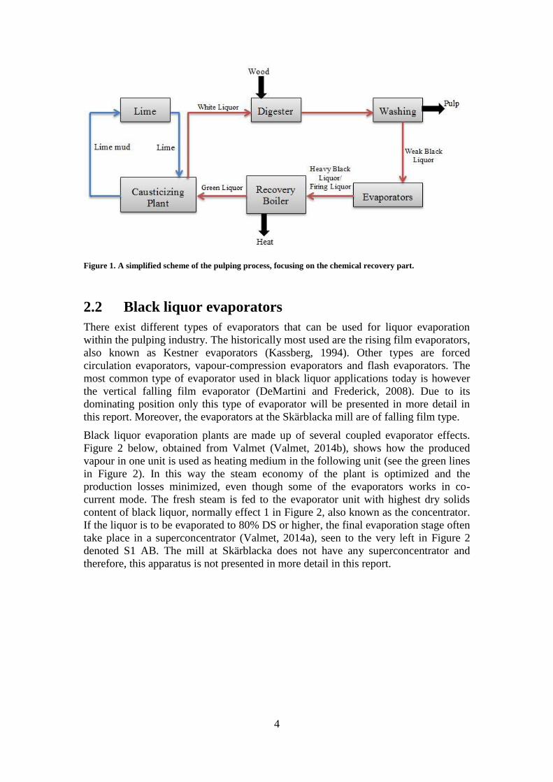
Figure 1. A simplified scheme of the pulping process, focusing on the chemical recovery part.

2.2 Black liquor evaporators

There exist different types of evaporators that can be used for liquor evaporation

within the pulping industry. The historically most used are the rising film evaporators,

also known as Kestner evaporators (Kassberg, 1994). Other types are forced

circulation evaporators, vapour-compression evaporators and flash evaporators. The

most common type of evaporator used in black liquor applications today is however

the vertical falling film evaporator (DeMartini and Frederick, 2008). Due to its

dominating position only this type of evaporator will be presented in more detail in

this report. Moreover, the evaporators at the Skärblacka mill are of falling film type.

Black liquor evaporation plants are made up of several coupled evaporator effects.

Figure 2 below, obtained from Valmet (Valmet, 2014b), shows how the produced

vapour in one unit is used as heating medium in the following unit (see the green lines

in Figure 2). In this way the steam economy of the plant is optimized and the

production losses minimized, even though some of the evaporators works in co-

current mode. The fresh steam is fed to the evaporator unit with highest dry solids

content of black liquor, normally effect 1 in Figure 2, also known as the concentrator.

If the liquor is to be evaporated to 80% DS or higher, the final evaporation stage often

take place in a superconcentrator (Valmet, 2014a), seen to the very left in Figure 2

denoted S1 AB. The mill at Skärblacka does not have any superconcentrator and

therefore, this apparatus is not presented in more detail in this report.

5

Figure 2. Typical process scheme for a pulp mill evaporation plant built by Valmet AB (Valmet, 2014b) .

At Skärblacka, the evaporation unit generating the liquor with highest DS is the

concentrator. This liquor is also denoted as heavy black liquor (HBL) or firing liquor

and has, at Skärblacka, a dry solids content of approximately 75%. To make the

evaporation more effective and to simplify cleaning, the concentrator is divided into

four units (1A, 1B, 1C and 1D). The different concentrator units operates in series on

the liquor side but are all heated by primary steam. Units 1A and 1B are connected via

a gap in a partition wall and the same is valid for units 1C and 1D, whilst there exists

circulation pipes between 1C-1B and 1A-1D. The liquor produced by effects 4-7 is

denoted, intermediate liquor and the liquor entering the concentrator intermediate

thick liquor. A more thorough description of the liquor flows and the concentrator

units is given in Section 2.4.

2.2.1 Falling film evaporators

The principle behind falling film evaporators is that liquor is fed to the top of the

evaporator unit and then falls down along the heating surfaces, evenly distributed over

the whole area (Kassberg, 1994). The heat transfer surface can be built up of either

lamellas or tubes, where the liquor for the latter one can be located either on the

outside or on the inside (Karlsson et al., 2014a). Then, driven by gravity, the liquor

forms a thin film on the surfaces and becomes partially evaporated on its way down

the lamellas/tubes. A schematic showing the liquor side of an evaporator effect

consisting of tubes is found in Figure 3. To ensure continuous flow of liquor and

stable operation there are always a buffer of liquor, a so called sump volume, at the

bottom of the evaporator. Another precaution to maintain sufficient wetting of the

heating surfaces is to have a high recirculation rate (Karlsson et al., 2014a). Falling

film evaporators are characterized by their high heat transfer coefficient and by short

contact time between the liquor and the heat transfer surface. The short contact time is

beneficial since it reduces the risk for fouling on the surfaces (Schmidl and Frederick,

1998).

6

Figure 3. General layout of an evaporator with heat transfer surfaces consisting of tubes. (Karlsson et al.,

2014a).

2.3 Fouling in black liquor evaporators

Black liquor contains many organic and inorganic compounds which, at high

concentration, have the potential to cause fouling on the heat transfer surfaces. The

origin of organic fouling is organic compounds like soap and fibers deposit on the

surfaces. They are however normally not the major contributor to fouling in black

liquor evaporators. Instead, crystallization of inorganic salts is believed to be the most

problematic aspect (Schmidl and Frederick, 1998). The onset of crystallization is

when the salts start to precipitate, and this occurs when the solubility limit is exceeded

(Shi, 2002). The formed crystals can either be located to the bulk liquor or adhere to

surfaces. If the latter occur, the crystals will form an insulating layer on the heating

surfaces that will reduce heat transfer. This type of fouling that origin from

precipitation of salts is known as scaling.

The scaling salts can be classified either as soluble or insoluble. Regarding the soluble

scales, sodium carbonate (𝑁𝑎2𝐶𝑂3) and sodium sulphate (𝑁𝑎2𝑆𝑂4) are most frequent.

According to Schmidl and Frederick (1998) the sodium content in black liquor is 18.4

wt. % of the dry content. This can be compared to a content of 409 ppm of the dry

content for the most common origin to insoluble scales, calcium. In the same report

by Schmidl and Frederick (1998) it is also revealed that most of the scaling problems

in black liquor evaporators today are due to sodium scaling. Within this thesis, only

scaling due to sodium salts is treated.

The high content of sodium salts in black liquor is one reason why these types of

scales are formed frequently. Another is the salts’ inverse solubility with temperature,

giving lower solubility closer to the heating surfaces (Gourdon, 2009). This implies,

based on the aspect presented above that precipitation only starts when the solubility

limit is exceeded, that the salts will precipitate near the surface and are therefore more

likely to crystallize on the surface than remain in the bulk.

7

The main origin of sodium carbonate and sodium sulphate is the reaction between the

wood raw material and the chemicals in the white liquor in the cooking process.

Depending on the relation between the two sodium salts in the black liquor, different

types of crystals will form. The solvent-free mole fraction is defined as (Gourdon,

2009):

𝑥 =

[𝑁𝑎2𝐶𝑂3]

[𝑁𝑎2𝐶𝑂3] + [𝑁𝑎2𝑆𝑂4]

(1)

Particulary two crystals have been found of importance for the scaling in black liquor

evaporators (Shi, 2002). These crystals are known as burkeite and dicarbonate. The

burkeite phase exists at mole fraction ranges in liquid phase of 0.22 to 0.83, whilst the

dicarbonate interval ranges from 0.833 to 0.9 mole fraction of carbonate in the

solution (Gourdon, 2009). A survey made by Frederick Jr et al. (2004)indicate that it

is in the dicarbonate region or in the region where both burkeite and dicarbonate

crystallize that the problems with scaling are most severe . Moreover, the majority of

evaporators operates with a black liquor having a 𝑁𝑎2𝐶𝑂3 composition within this

region, i.e. with 0.68<x<0.89 (Schmidl and Frederick, 1998, Frederick Jr et al., 2004).

For sodium salts, the solubility limit is exceeded when the dry solids content reaches

above approximately 50 % (Shi, 2002). The only evaporator effects with this high DS

content are the concentrator (effect 1), the superconcentrator if available, and

sometimes also effect 2 (Karlsson et al., 2014a).

Regarding insoluble scales, calcium carbonates constitute the biggest share but it

might also include aluminium silicates and calcium silicates. Other types of fouling

that can take place in black liquor evaporators origin from soap and fiber. Calcium

scales have in contrast to sodium scales low solubility in water and the formed scales

are also harder. Calcium scaling can be avoided by heating the liquor before it enters

the evaporator. If dissolved calcium enters the evaporation units it will form complex

together with the dissolved organic compounds and adhere to the surfaces. By

preheating, the calcium will only exist as calcium carbonate crystals when the liquor

enters the evaporators and those crystals will not contribute to any scaling (Shi, 2002).

Since they mainly exist within the bulk phase neither soap or fiber is a primary scaling

agent, but their presence and interactions with other compounds may enhance the

fouling rate (Clay, 2008). Fibers can plug evaporators and prohibit even distribution

of the liquor on heating surfaces leading to acceleration of other scaling mechanism.

Soap contains high amounts of both calcium and fiber which might cause increased

calcium scaling and increased risk for fiber plugging. To minimize the problems with

soap- and fiber fouling, these substances are removed before the liquor enters the

evaporator.

8

2.4 Evaporator washing procedure at Skärblacka

Washing is the measure to remove scales from the heating surfaces. Since it is only

the evaporator units with highest dry solids content that are exposed to severe fouling,

it is those which are desired to wash frequently. In May 2013, a new evaporator

facility went into operation at BillerudKorsnäs’ mill at Skärblacka (Back, 2014). The

installation was carried out in several steps and the whole evaporator unit was built

and delivered by Valmet. This thesis focuses on the cleaning of the concentrator unit

at Skärblacka, consisting of four individual units in series, where the dry solids

content after the last unit normally reaches ~75% (Valmet, 2014a). However, the main

features are similar to evaporator washing at other pulp mills as well. The heating

surfaces for all evaporator effects at Skärblacka are built up of tubes, and for effect 2-

7 is the liquor located inside the tubes whilst it flows on the outside for the

concentrator (Valmet, 2014a).

During normal operation, all concentrator units are used for evaporation of the

incoming intermediate thick black liquor (IMTHL) into heavy black liquor (HBL).

Figure 4 below shows pathways for the black liquor (red lines) and the feed liquor

(yellow lines) in the concentrator during normal operation. The feed liquor (FL) is the

same liquor as the one that enters the evaporation stage, i.e. the weak black liquor.

During normal operation, the feed liquor is led directly to the flash tank without

passing through any evaporator. Always having a small flow of liquor in the pipe

ensures smooth operation and prevents clogging.

There are two alternatives how the intermediate thick black liquor produced by

evaporator effect 2 can be fed to the concentrator under normal operation, either, as in

Figure 4, to unit 1B or to unit 1D (Figure 6). The two scenarios are referred to as

liquor order B-A-D-C and D-C-B-A respectively.

Figure 4. Simplified picture of the concentrator under normal operation, obtained from Valmet (Valmet,

2014b). The black liquor is fed to unit 1B, giving the liquor order B-A-D-C. White vales indicate open pipe

and black closed pipe.

9

The major indication that a wash is needed is that the overall heat transfer coefficient,

the 𝑈-value, drops below a given limit (Valmet, 2014a). When this occur the

automatic wash sequence is initiated from the control system by an operator. The first

that happens when a wash sequence is started is that the liquor level in the unit to be

washed is reduced. This is done by ramping down the reference value for the liquor

sump level. Secondly, via several changes in valve position the liquor flows are then

altered; intermediate thick black liquor is pumped past the unit to be washed and into

the next one. The feed liquor is pumped into the evaporator and begins to circulate,

and is finally led out from the evaporation plant via the flash (“Heavy liquor flash 2”

in Figure 5) (Valmet, 2014a). Figure 5 shows liquor flows and valve positions for

wash of unit 1D-1C, but the procedure is similar for cleaning of unit 1A-1B as well.

Figure 5 also shows that the two concentrator units that are not to be washed, i.e. 1B

and 1A in this case, remains in normal operation and continues to produce heavy

black liquor. However, since only two of the four concentrator units now produce

heavy black liquor, the size of the intermediate thick black liquor flow to the

concentrator is decreased compared to under normal operation. The amount of liquor

leaving evaporator unit 2 is however unchanged, generating larger quantities of liquor

to an intermediate liquor storage tank located after effect 2 compared to during normal

operation (Valmet, 2014a). It is desired to keep the amount of vapour from the

concentrator (“Steam to effect 2” in Figure 4-Figure 6) at a constant level to ensure

stable operation of the other evaporator effects in the plant, independent of if wash

occurs or not. Therefore, during cleaning, the steam supply (“Fresh steam” in Figure

4-Figure 6) is redistributed with a higher feed to the units in normal operation, since

they have a higher load, and a lower feed to the units being cleaned (Karlsson et al.,

2014a). Also this redistribution of steam during wash sequence occurs automatically

by the control system. Since the feed of steam to the units producing heavy liquor is

increased during wash and the flow rate of the liquor is lower, the quality of the heavy

liquor is the same as under normal operation when all four units contributes to the

evaporation, i.e. the same DS is reached.

Figure 5. Simplified picture of a washing sequence of the concentrator. The feed liquor is fed to unit 1D

meaning that unit 1D and 1C is being washed. Unit 1B and 1A remains in normal operation and produces

heavy black liquor (Valmet, 2014b).

10

The wash lasts until the heating surfaces are considered clean from scales. Normal

time for a wash sequence at the Skärblacka mill is around one hour (Redeborn, 2014).

Once the wash is finished, the wash liquor is released out of the unit by ramping of

the sump level. The wash liquor flow is reduced to its original value and the shut-off

valves for wash liquor are returned to their normal position, redirecting the flow

straight to the flash tank again. The intermediate black liquor is led back into the

cleaned unit and the steam-and liquor flows return to their original values. Finally, the

level in the cleaned unit is raised and evaporation returns to normal operation

(Valmet, 2014a).

Typically, the liquid order is changed each time a wash sequence is completed (e.g.

from B-A-D-C to D-C-B-A). Figure 6 illustrates the directions of the liquor flows

when the evaporation returns to normal operation after wash of unit 1D-1C. At

Skärblacka, each unit is washed approximately once every third day (Redeborn,

2014).

Figure 6. Simplified picture of the concentrator when it is back to normal operation after the wash

sequence. The black liquor is now fed to unit 1D, giving the liquor order D-C-B-A. A liquor shift has

occurred compared to before the wash sequence.

A picture showing the concentrator during different stages of the evaporation process

together with more thorough explanations can be found in Figure A in Appendix A.

11

3 The Cleaning Model

One important tool in this thesis has been a model that simulates evaporator cleaning

by describing scale dissolution and mass flows over time. The original model

simulates cleaning of one single evaporator unit, but the set-up at the Skärblacka mill

did not enable sample collection representing this. Therefore one part of this thesis

has been to implement modifications to the original model. This chapter will present

the most essential parts of the original model. For a complete review of the original

model and how the it was developed refers to two articles by Karlsson et. al, (2014b,

2014a). The required modifications to make the model suitable for comparison with

the Skärblacka mill and motivations behind them are found in Section 4.1 of this

report.

The scale dissolution process implies mass transfer from a surface to a liquid and is,

depending on the circumstances, controlled by either diffusion or reaction. The

controlling mechanism is the transport phenomenon that poses largest resistance

towards mass transfer, with exception the special case when both resistances are of

equally size. In situations where salt scales are dissolved, the reaction comprises

breaking of crystal lattice and generation of ions. It has been found that dissolution of

sodium scales in large-scale black liquor falling film evaporators, which is the

situation modelled in this study, is rate-controlled by diffusion (Karlsson et al.,

2014b).

3.1 Film theory

Within the film theory concept, a thin fictitious film is assumed to be present close to

the scale surface. Depending on the flow behaviour, whether it is in the laminar or

turbulent region, the film will have different characteristics. For a more turbulent film,

a boundary will form that divides the film into a laminar boundary layer and a

turbulent bulk section (Figure 7). For the film theory to be applicable for simulation of

scale dissolution, the bulk phase is assumed to be perfectly mixed (Welty et al., 2001).

According to the film theory, all mass transfer resistance exists in the diffusion film,

𝛿𝑑, and the mass transport occurs only through molecular diffusion. When the scales

start to dissolve they will diffuse through the diffusion film, but once they have passed

the boundary between the diffusion film and the bulk flow they will be considered as

part of the bulk flow with a uniform concentration. The resistance to mass transfer in

horizontal direction can thus be neglected in the bulk flow. At the scales surface the

concentration is equal to the saturation concentration at the current temperature, 𝑐∗.

12

Figure 7. Schematic sketch of the concentration profile based on the film theory concept.

One important criteria for the film theory model to be appropriate is that the diffusion

film must be considerably thinner than the total thickness of the falling film, 𝛿𝑡𝑜𝑡.

According to the film theory, the dissolution rate (i.e. the mass transfer per area from

scale surface into the liquid) for a diffusion controlled dissolution process with

turbulent bulk flow can be expressed as follows:

𝐽𝑥 = 𝐷𝐴𝐵

𝜕𝑐

𝜕𝑥≈ 𝐷𝐴𝐵

∆𝑐

∆𝑥=

𝐷𝐴𝐵

𝛿𝑑∆𝑐 = 𝑘𝑚(𝑐∗ − 𝑐𝑏) (2)

Equation (2) is known as Fick’s law or the Fick rate equation and describes the

molecular mass transfer per area from the scale surface into the liquid (Welty et al.,

2001). The simplifications seen in the equation are justified by the film theory. In this

case, index x indicates the axis perpendicular to the surface, 𝐷𝐴𝐵 is the diffusion

coefficient and 𝜕𝑐

𝜕𝑥 is the true concentration gradient. 𝑘𝑚 is the mass transfer

coefficient and 𝑐∗ − 𝑐𝑏 is the difference between the solubility limit and the bulk

concentration, i.e. the driving force. 𝛿𝑑 is the thickness of the fictive diffusion film.

As given by Equation (2) the dissolution rate depends on the mass transfer coefficient

and the difference in concentration between saturation and the bulk flow. As long as

the bulk concentration is lower than the solubility limit, scales will be dissolved when

the wash liquid falls along the scaled surfaces. Since more and more scales dissolves

when the contact time increases, also the bulk concentration will increase. This

implies reduced driving force for dissolution when the wash liquid falls along the

surface, approaching zero when the bulk reaches saturation.

3.2 Original model construction

One important aid for the establishment of the cleaning model was experiments

performed at a pilot evaporator plant. Aside from awareness learnt about general

behaviour, knowledge gained from these experiments was also used to give data

needed in the modelling tool. A previous master thesis performed at the division of

Heat and Power Technology by Broberg and Åkesjö (2012) investigated the scale

dissolution rate and found that it followed a first order diffusion-reaction. The first

prototype of the cleaning model was developed based on their findings.

13

To make the model a credible representation of reality not just the flow over the

heating surfaces is simulated, also the amount of liquor in the recirculation loop and

the time delay this causes is considered. Another important aspect is the position of

the outflow. The model enables simulation for both the possible outflow positions

seen in Figure 3, Section 2.2.1, i.e. after the recirculation pump and in the sump. Due

to lack of stirring, it might not be legitimate to consider the volume of liquor in the

sump as perfectly mixed. To account for the non-ideal mixing the sump volume is

divided into two perfectly mixed tanks in series.

The pilot evaporator is equipped with sight glasses at three different heights, enabling

the scale thickness to be determined. However, experiments performed within an

earlier master thesis showed very inconsistent results and concluded that it is not

possible to construct a general scale distribution method (Petterson and Öhrman,

2013). Some typical features were however noticed; among others that the scales

normally were thickest at the bottom of the evaporation tubes (Gourdon, 2009). The

model is built up in a way that enables this knowledge to be taken into consideration

since the scale thickness is defined at all heights of the evaporator.

The cleaning model simulates a wash sequence by taking small time steps. The

evaporator tube is divided into short tube segments and the scale distribution for each

segment and time step is calculated. The initial scale thickness is an input that can be

chosen freely for different heights of the tube, and interpolation is then used to

allocate the thicknesses for the other parts of the tube. All physical properties are

assumed to be constant within each segment. Mass balances are used to determine the

amount salt transported out by the wash liquid based on the amount of salt dissolved

from the tube. Another mass balance ensures that the assumed scale distribution adds

up to the total amount of dissolved scales, i.e. the amount dissolved in all segments.

Equation (2) shows that the mass transfer coefficient 𝑘𝑚 is a key parameter for the

determination of the dissolution rate. 𝑘𝑚 accounts for diffusion from the solid surface

to the bulk, and does therefore also include the diffusion coefficient 𝐷𝐴𝐵, and has been

determined from the Chilton-Colburn analogy (Welty et al., 2001). This analogy

enables estimation of the mass transfer coefficient from the heat transfer coefficient.

In the cleaning model, correlations from Schnabel and Schünder (1980) were used to

estimate the heat transfer coefficient (Karlsson et al., 2014b). For all details how the

mass transfer coefficient as well as all other physical properties needed in the

calculations were obtained, see Karlsson et al (2014a/b).

Input parameters that are to be defined to create specific cleaning sequences are;

initial scale distribution, steam- and liquor flows, temperatures in the different stages,

initial dry solids content in the evaporator units, wash liquor properties, and design

data including diameter, length and number of tubes.

One important feature for the cleaning model is that it simulates the cleaning of one

tube and then assumes that the cleaning procedure is identical for all tubes within the

evaporator.

15

4 Methodology

The approach for this thesis has been both analytical and experimental. The analytical

part includes, in addition to the initial literature review, also the re-building of the

already existing cleaning model presented in Section 3.2. The experimental part

comprises a full scale wash experiment at the Skärblacka mill, with collection of both

online data and liquor samples.

4.1 Model adaptions to the Skärblacka case

In the beginning of the thesis, it was not obvious that adaptions of the existing

cleaning model were needed. Even though the concentrator at Skärblacka consists of

four units connected two-and-two, the hope were to collect samples at the

recirculation pipe of the first unit the liquor enters in the concentrator, which would

mean that samples of both the inflow and outflow of liquor to this unit was collected

(see Figure 8 below). This procedure of sampling would have given good

correspondence with the original cleaning model. However, during the visit to

Skärblacka it was discovered that the valves enabling sampling at the recirculation

pipe were unpractical located close to the floor and the safety could not be guaranteed

if samples were to be collected at this position.

Figure 8. Flow sheet showing wash sequence of unit 1D-1C. The cross-shaped markers indicate desired

extraction positions (blue=collection of inflow, green=collection of outflow) (Valmet, 2014b).

A more convenient way to collect sample of the liquor that have passed the

concentrator unit can be seen in Figure 9. The liquor has in this case passed not only

two concentrator units, but also a flash. The flash reduces the temperature and

pressure of the liquor making it much safer to handle. The liquor entering the

concentrator units to be washed during wash sequence is from now on denoted as feed

liquor (FL) whilst the liquor samples collected after the flash is called wash liquor

(WL).

16

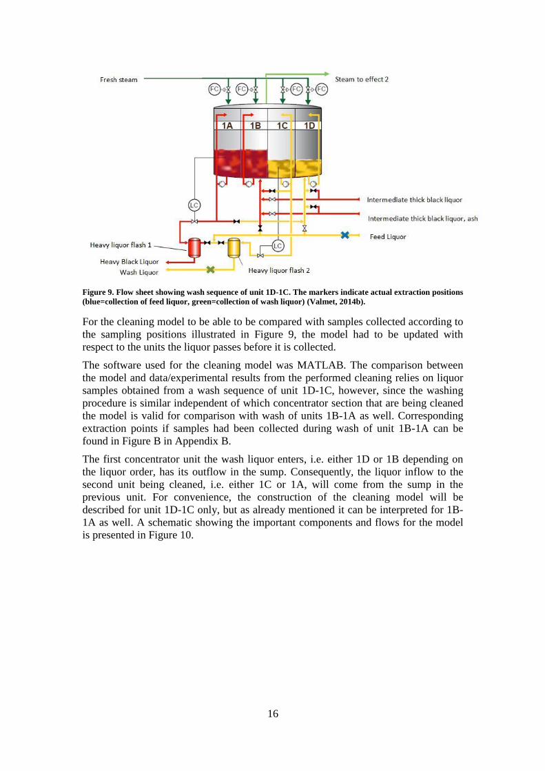
Figure 9. Flow sheet showing wash sequence of unit 1D-1C. The markers indicate actual extraction positions

(blue=collection of feed liquor, green=collection of wash liquor) (Valmet, 2014b).

For the cleaning model to be able to be compared with samples collected according to

the sampling positions illustrated in Figure 9, the model had to be updated with

respect to the units the liquor passes before it is collected.

The software used for the cleaning model was MATLAB. The comparison between

the model and data/experimental results from the performed cleaning relies on liquor

samples obtained from a wash sequence of unit 1D-1C, however, since the washing

procedure is similar independent of which concentrator section that are being cleaned

the model is valid for comparison with wash of units 1B-1A as well. Corresponding

extraction points if samples had been collected during wash of unit 1B-1A can be

found in Figure B in Appendix B.

The first concentrator unit the wash liquor enters, i.e. either 1D or 1B depending on

the liquor order, has its outflow in the sump. Consequently, the liquor inflow to the

second unit being cleaned, i.e. either 1C or 1A, will come from the sump in the

previous unit. For convenience, the construction of the cleaning model will be

described for unit 1D-1C only, but as already mentioned it can be interpreted for 1B-

1A as well. A schematic showing the important components and flows for the model

is presented in Figure 10.

17

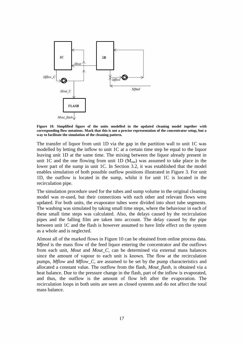
Figure 10. Simplified figure of the units modelled in the updated cleaning model together with

corresponding flow notations. Mark that this is not a precise representation of the concentrator setup, but a

way to facilitate the simulation of the cleaning pattern.

The transfer of liquor from unit 1D via the gap in the partition wall to unit 1C was

modelled by letting the inflow to unit 1C at a certain time step be equal to the liquor

leaving unit 1D at the same time. The mixing between the liquor already present in

unit 1C and the one flowing from unit 1D (Mout) was assumed to take place in the

lower part of the sump in unit 1C. In Section 3.2, it was established that the model

enables simulation of both possible outflow positions illustrated in Figure 3. For unit

1D, the outflow is located in the sump, whilst it for unit 1C is located in the

recirculation pipe.

The simulation procedure used for the tubes and sump volume in the original cleaning

model was re-used, but their connections with each other and relevant flows were

updated. For both units, the evaporator tubes were divided into short tube segments.

The washing was simulated by taking small time steps, where the behaviour in each of

these small time steps was calculated. Also, the delays caused by the recirculation

pipes and the falling film are taken into account. The delay caused by the pipe

between unit 1C and the flash is however assumed to have little effect on the system

as a whole and is neglected.

Almost all of the marked flows in Figure 10 can be obtained from online process data.

Mfeed is the mass flow of the feed liquor entering the concentrator and the outflows

from each unit, Mout and Mout_C, can be determined via external mass balances

since the amount of vapour to each unit is known. The flow at the recirculation

pumps, Mflow and Mflow_C, are assumed to be set by the pump characteristics and

allocated a constant value. The outflow from the flash, Mout_flash, is obtained via a

heat balance. Due to the pressure change in the flash, part of the inflow is evaporated,

and thus, the outflow is the amount of flow left after the evaporation. The

recirculation loops in both units are seen as closed systems and do not affect the total

mass balance.

18

The cleaning model was expanded with a section calculating the heat transfer

coefficient, 𝑈-value. Each scale distribution generates a certain 𝑈-value and the

resistance towards heat transfer is increased with thicker layer of scales. Thus, the

𝑈-value attains a higher value if the tube is clean than if it is covered with scales.

However, one value of the heat transfer coefficient can represent several different

distributions.

The heat transfer coefficient was calculated according to Equation (3) (Gourdon,

2009):

𝑈𝑓𝑜𝑢𝑙 =

∑ 𝐴𝑖 (1

𝑈𝑐𝑙𝑒𝑎𝑛+

𝑑𝑓𝑜𝑢𝑙 · ln (𝑑𝑓𝑜𝑢𝑙

𝑑𝑜)

2 ∙ 𝑘𝑤,𝑓𝑜𝑢𝑙)𝑖

𝑖=1

−1

𝐴𝑡𝑜𝑡

(3)

where i is the number of tube segments, 𝐴𝑖 is the area of each segment and 𝐴𝑡𝑜𝑡 is the

total area of the tube. The value of 𝑈𝑐𝑙𝑒𝑎𝑛indicates the heat transfer when the

evaporator is cleaned and can be obtained from online process data. 𝑑𝑜is the tube

outside diameter and 𝑑𝑓𝑜𝑢𝑙is the total diameter of tube and scales, calculated within

the model. 𝑘𝑤,𝑓𝑜𝑢𝑙 is the thermal conductivity of the of the fouling material and is

equal to 1.73 𝑊

𝑚∙𝐾 (Smith, 2000). 𝑈𝑓𝑜𝑢𝑙 refers to the heat transfer for the fouled

evaporator. For the purpose used in this study, the parameter of interest 𝑈 is equal to

𝑈𝑓𝑜𝑢𝑙.

Within the cleaning model, the boiling point rise (BPR) was also calculated. Boiling

point rise is the temperature difference between the boiling point of pure water and

the boiling point of the liquor at the same pressure (Frederick, 1997). In the model,

the following correlation was used to calculate BPR of the liquor (Wennberg, 1990):

𝐵𝑃𝑅 = 1.08 ∙ 𝑀𝑜𝑙𝑎𝑙𝑖𝑡𝑦 − 0.8 (4)

where “molality” is the molality of sodium and potassium in [𝑚𝑜𝑙𝑒

𝑘𝑔𝐻2𝑂]. The relation is

only valid for BPR’s below 10 degrees (Wennberg, 1990). The validity of the used

BPR model was confirmed by comparing it with two other models. The other models

were valid for pure liquor only, whilst the one used also considers salts. Since the

three models gave almost identical results when applied on pure liquor, the used BPR

model was accepted and regarded as valid for the purpose of these analyses.

19

4.2 Data collection

One effective approach to monitor the wash is to study the change in salt content. The

change in salt content for the liquor collected after the flash, i.e. for the wash liquor, at

different times during the wash reveals how much of the scales on the heating

surfaces that have been dissolved into the ingoing feed liquor. The variation in salt

content can be visualised by the changes in dry solids content, boiling point rise and

salt concentration during the wash. In this thesis, salt concentration refers to the

concentration of sulphate, carbonate and of the sodium associated to the scales, i.e. the

salts contributing to fouling. The amount of sodium associated to the scales was

calculated from the amounts of sulphate and carbonate utilizing the molar ratio.

To be able to investigate how these parameters varied during the wash it was

necessary to collect wash data, which was done during a full scale test at the

Skärblacka pulp and paper mill. The wash data used as basis for the comparison with

the cleaning model included both collection of liquor samples from the evaporator and

gathering of online process data from the mill’s control system.

21 liquor samples were collected at the locations marked in Figure 9 above and sent to

laboratory for analysis. Relevant analyses were dry solids content and content of

potassium(𝐾), sodium(𝑁𝑎), sulphate (𝑆𝑂4) and carbonate (𝐶𝑂3). Since the liquor of

highest interest is the one that have passed through the fouled concentrator units, i.e.

the wash liquor, focus was to collect samples at this site. Regarding the feed liquor,

the flow is assumed to be constant both regarding flow rate and composition during

the wash. However, as a precaution and to verify this, a number of samples were

collected at that location as well.

The control system at Skärblacka provided online process data from both before,

during and after the wash. Parameters of interest were in particular boiling point rise

and 𝑈-value for the washed units, dry solids content in the heavy liquor flashes, and

both pressure and temperatures for the flash and all concentrator units.

4.3 Sample analysis

The majority of the analyses were performed by external laboratories. As already

mentioned the properties of interest were dry solids content and content of sodium,

sulphate, carbonate and potassium. Some of the samples were analysed by the

laboratory at Skärblacka, whilst others were sent to the company MoRe Research.

However, for some samples, analyses of the dry solids content were also performed at

Chalmers. Those analyses followed the test method TAPPI T 650 om-09. An

explanation to how the salt concentration was calculated from the laboratory results

can be found in Appendix C.

21

5 Design Data and Process Data

The model requires input data both concerning evaporator design as well as more

specific simulation settings and operation conditions. The most important input

parameters defined in the model are shown in Table 1 and Table 2.

Table 1. Evaporator design data and liquor volumes used in the cleaning model.

HEAT TRANSFER SURFACE

Tube length, L 12 m

Outer tube diameter, d0 0.032 m

Total area, Atot 2200 m2

Number of tubes in each concentrator unit, NumTubes 1800

LIQOUR VOLUMES

Total liquor volume in sump, equal for both units. Vsump 3.7 m3

Total liquor volume in recirculation pipe, equal for both units,

Vcirk

7 m3

Total liquor volume on tub surface, equal for both units, Vtub 3 m3

The heat transfer surface data are defined according to the design data of the

evaporator at Skärblacka. The liquor volumes assigned to recirculation pipe and tube

surface are normally small compared to the total wash liquor flow and have limited

influence on the simulations. The sump volume during cleaning was calculated from

design data. At normal operation, the liquor level occupies 66% of the mesured

height in the space below the tubes, corresponding to 34 m3 for the whole

concentrator. During wash, the liquor level is reduced to 30%. By knowing the design

data for the concentrator, the sump volume for each of the four concentrator units was

determined to approximately 3.7 m3.

Some of the necessary input parameters in the cleaning model were obtained from

online process data collected from the control system during the wash, see Table 2.

22

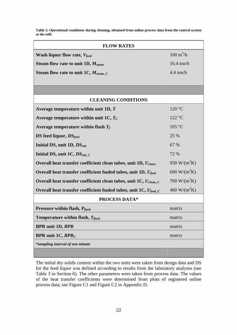
Table 2. Operational conditions during cleaning, obtained from online process data from the control system

at the mill.

FLOW RATES

Wash liqour flow rate, Vfeed 100 m3/h

Steam flow rate to unit 1D, Msteam 16.4 ton/h

Steam flow rate to unit 1C, Msteam_C 4.4 ton/h

CLEANING CONDITIONS

Average temperature within unit 1D, T 120 °C

Average temperature within unit 1C, TC 122 °C

Average temperature within flash Tf 105 °C

DS feed liquor, DSfeed 25 %

Initial DS, unit 1D, DSinit 67 %

Initial DS, unit 1C, DSinit_C 72 %

Overall heat transfer coefficient clean tubes, unit 1D, Uclean 930 W/(m2K)

Overall heat transfer coefficient fouled tubes, unit 1D, Ufoul 690 W/(m2K)

Overall heat transfer coefficient clean tubes, unit 1C, Uclean_C 700 W/(m2K)

Overall heat transfer coefficient fouled tubes, unit 1C, Ufoul_C 460 W/(m2K)

PROCESS DATA*

Pressure within flash, Pflash matrix

Temperature within flash, Tflash matrix

BPR unit 1D, BPR matrix

BPR unit 1C, BPRC matrix

*sampling interval of one minute

The initial dry solids content within the two units were taken from design data and DS

for the feed liquor was defined according to results from the laboratory analyses (see

Table 3 in Section 6). The other parameters were taken from process data. The values

of the heat transfer coefficients were determined from plots of registered online

process data; see Figure C1 and Figure C2 in Appendix D.

23

6 Laboratory Results and Discussion

As mentioned earlier in the report the analysis of collected liquor samples were

performed at two different laboratories, MoRe Research and the laboratory at the

Skärblacka mill. Table 3 below assembles the most important lab results and clarifies

which samples that were analysed at which laboratory. A complete compilation of the

results for all liquor samples can be found in Table B in Appendix E.

Online process data showed that feed liquor was led into unit 1D at approximately

13:43. This change of liquor type at the inlet to unit 1D, from black liquor to feed

liquor, indicates that the wash has started. Based on this the cumulative time, i.e. the

time since the wash started, was determined for each collected sample. The samples of

heavy black liquor (HBL) and wash liquor (WL) were collected at the same location

after the flash (see green marker in Figure 9), but HBL before the wash was initiated

and WL during the wash. The feed liquor samples (FL) was collected at the inlet to

the concentrator (blue marker in Figure 9).

Table 3. Compilation of relevant lab results. The indexes for liquor type refers to Heavy Black Liquor

(HBL), Feed Liquor (FL) and Wash Liquor (WL). Samples marked with dark grey have been analysed by

MoRe Research and light grey samples was evaluated by the laboratory at Skärblacka. Some DS-analyses

were performed at Chalmers. Cum. Time (cumulative time) indicates number of minutes passed since wash

started at 13:43.

Sample Cum. time

Liquor

type

SO4 CO3 K Na DS DS

Chalmers

[𝒎𝒊𝒏] [𝒈

𝒌𝒈𝑫𝑺⁄ ] [

𝒈𝒌𝒈𝑫𝑺

⁄ ] [𝒈



⁄ ] [% ] [% ]

1 - HBL 51.3 50.4 13.7 194.3 76.6

2 - HBL 41.7 126 201 75.3

3 - FL 12.8 48.8 12.4 194.0 25 24.6

5 - FL 13.4 103 177 26

6 16 WL 185 56.1

7 21 WL 31.6 55.5 13.9 210.4 50

9 31 WL 56.2 162 207 43.7

10 36 WL 42.7 83.6 12.0 212.5 41.7

12 48 WL 38.6 80.7 12.2 211.8 37.3

14 56 WL 205 34.7

15 64 WL 29.6 70.2 12.2 201.4 34.5

16 72 WL 31.6 67.7 12.3 201.2 33.3

19 94 WL 21.7 62.6 12.5 194.7 32.3 31.6

21 99 WL 196 31.1

24

The data presented in Table 3 indicate that the values are influenced by where they

were analysed. For example, sample number 1 and 2 which were collected at the same

location at the same time has good agreement in DS but large deviation regarding

CO3-content. The trend that the laboratory at Skärblacka predicts higher content of

CO3 than MoRe Research is general for all evaluated samples, and is concluded by the

comparison of sample number 3 with 5, and 9 with 10.

One measure to determine if the evaporator is cleaned is to compare the salt content in

the wash liquor with the content in the feed liquor. Since the scales consist of sodium

sulphate and sodium carbonate, the content of these substances are expected to

increase when scales are dissolved. Then, when all scales have been dissolved from

the heating surfaces, will further wash instead lead to that the liquor becomes more

and more diluted and that the salt content decreases. When the liquor has been diluted

enough and all dissolved salts are discharged from the liquor, the salt content within

the wash liquor should be equal to the salt content in the feed liquor. In other words, if

the content of a specific scaling substance in the wash liquor is similar to the content

of the same substance in the feed liquor, the wash can be considered finished. This

reasoning is only valid if the concentrations are expressed as per kilogram DS.

Otherwise, if the results also include the amount of water and are expressed as per

kilogram total liquid, the results will be influenced by the rate of evaporation.

The sodium content in sample 3 and 19 are almost identical, indicating that all scales

have been removed from the evaporator. However, the sulphate and carbonate

contents are much higher in sample 19 than in sample 3, indicating that the evaporator

is not clean. Since potassium is not present in the scales formed at the heating

surfaces, the amount should be constant during the wash. This expected behaviour is

confirmed by the results presented in Table 3. Another reason why potassium was

analysed is that its molality is used to determine BPR.

The results of dry solids content are much more consistent than the analysis of the

different salts. Table 3 shows how the DS decreases with reasonable steps as the wash

continues. The agreement between the laboratories’ results and the analysis performed

at Chalmers is also high.

25

7 Modelling Results and Discussion

This section of the report presents the findings from the simulations. Different input

parameters within the washing model have been varied and their influence on the

agreement with online process data and lab results was studied. The analyses focused

on finding how different parameters affect the wash and how they can be varied to

obtain as efficient wash as possible. A second goal was to predict how the scales were

distributed within the evaporator.

For the cases where scale distribution is the input parameter studied, the model

enables different scale thicknesses to be defined for each unit.

7.1 Boiling point rise

The boiling point rise (BPR) from the model is plotted together with the values for

BPR obtained from online process data. For the model, BPR is calculated based on

molality of sodium and potassium in the liquor, see Equation (4) in Section 4.1. Since

the obtained process data only included BPR for unit 1D and 1C and not for the flash,

the BPR for the same locations is calculated by the model.

Since the model calculates BPR based on molality, and molality is proportional to the

amount of dissolved scales, the BPR over time is affected by time it takes to dissolve

the scales. This in turn is dependent on the scale distribution. Therefore, in an attempt

to evaluate if BPR is a good parameter to follow for prediction of the wash progress,

the scale thickness in the two units was adjusted.

Table 4 below shows how the scale distributions were defined for five different

simulations denoted SD1-SD5. The results of the simulations are presented in Figure

11-Figure 13. The explanation to the uneven distribution in height for the defined

scale thicknesses and to why the tubes were assigned a thicker layer of scales near the

bottom is that earlier studies shows that the amount of scales normally is greater on

the lowest part of the evaporator tubes.

There might be difficult to see how the simulations in Table 4 are related to each

other, and the explanation to their different scale distributions is that SD2 was defined

based on the knowledge learnt from the results of simulation SD1, SD3 based on the

results of SD2 and so on. The argumentation behind the changes made in scale

distribution from one simulation to the next is presented later on in this section, but it

should be clarified that all changes aimed to improve the agreement between wash

model BPR and BPR from process data. The purpose with comparing simulation

SD1-SD5 with each other is to learn how different defined scale distributions affect

the wash model BPR.

26

Table 4. Defined scale thicknesses for different simulations. Height refers to height in meters from the

bottom of the evaporator tube with a total height of 12 meters and scale thickness is the thickness of the

scaling layer on the outside of the tube in millimeters.

HEIGHT [m] SCALE THICKNESS [mm]

SD1 SD2 SD3 SD4 SD5

1D 1C 1D 1C 1D 1C 1D 1C 1D 1C

12 0.1 0.1 0.1 0.1 0.1 0.01 0.1 0.01 0.1 0.01

6 0.1 0.1 0.1 0.1 0.1 0.01 0.1 0.01 0.1 0.01

1 0.5 0.5 0.5 0.3 0.5 0.01 0.5 0.01 0.5 0.01

0.5 3 2 3 2 3 0.01 3 0.01 3 0.01

0.3 8 5 8 5 5 0.01 5 0.01 8 0.01

0.2 11 5 11 5 5 0.01 10 0.01 11 0.01

0.1 14 8 14 8 5 0.01 10 0.01 14 0.01

0.05 17 10 20 10 20 0.01 30 0.01 40 0.01

0.02 17 15 20 15 20 0.01 30 0.01 40 0.01

0 17 15 20 15 20 0.01 30 0.01 40 0.01

Figure 11. Boiling point rise when the scale thickness for the model is set according to SD4. Dashed lines

indicate model and solid lines process data. The BPR in unit 1D is shown as black lines whilst green lines

represents unit 1C.

Figure 11 above shows the BPR variation during wash when the model is assigned

scale distributions according to simulation SD4. Of the five cases SD1-SD5, this

distribution was found to give the overall best agreement between BPR variation

27

during wash sequence for model and process data. For both units, the model is more

alike process data early in the wash sequence. It can also be seen that unit 1D follows

process data better than unit 1C between minutes ~40-75 and that unit 1C has better

agreement than unit 1D when the wash is finished. The x-axis is limited to 102

minutes, corresponding to the time the wash was terminated by the operator and

liquor flows changed back to normal operation. Also the model indicates that the

amount of salts in the liquor stabilises after little more than 100 minutes, illustrated by

that the lines showing BPR for the model flattens out.

Approximately 65 minutes into the wash, a small twist can be observed on the line

showing wash model BPR for unit 1D. The twist indicates that the cleaning is finished

and that only dilution of the liquor occurs after this point. This reasoning is supported

by the results showed in Figure 12, where the length of scales is presented.

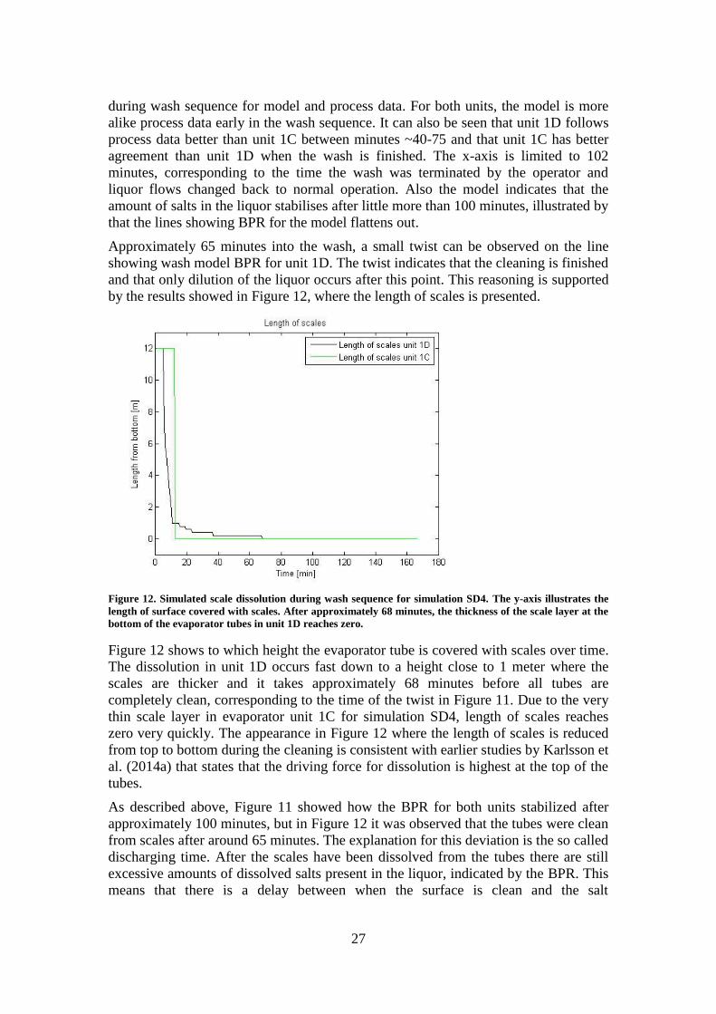
Figure 12. Simulated scale dissolution during wash sequence for simulation SD4. The y-axis illustrates the

length of surface covered with scales. After approximately 68 minutes, the thickness of the scale layer at the

bottom of the evaporator tubes in unit 1D reaches zero.

Figure 12 shows to which height the evaporator tube is covered with scales over time.

The dissolution in unit 1D occurs fast down to a height close to 1 meter where the

scales are thicker and it takes approximately 68 minutes before all tubes are

completely clean, corresponding to the time of the twist in Figure 11. Due to the very

thin scale layer in evaporator unit 1C for simulation SD4, length of scales reaches

zero very quickly. The appearance in Figure 12 where the length of scales is reduced

from top to bottom during the cleaning is consistent with earlier studies by Karlsson et

al. (2014a) that states that the driving force for dissolution is highest at the top of the

tubes.

As described above, Figure 11 showed how the BPR for both units stabilized after

approximately 100 minutes, but in Figure 12 it was observed that the tubes were clean

from scales after around 65 minutes. The explanation for this deviation is the so called

discharging time. After the scales have been dissolved from the tubes there are still

excessive amounts of dissolved salts present in the liquor, indicated by the BPR. This

means that there is a delay between when the surface is clean and the salt

28

concentration has returned to the value for pure black liquor, denoted discharging

time.

Another observation made from Figure 11 was that for the process data, the BPR in

the end of the wash is higher for unit 1D than unit 1C. This indicates that the online

process data cannot be completely reliable. Since the concentrator units are connected

in series the concentration of the liquor is higher in unit 1C than in 1D due to

evaporation, and this also implies higher BPR. In that respect, some deviation

between model and the online process data can be expected.

The results of simulation SD1, SD2, SD3 and SD5 are presented in Figure 13a-Figure

13d.

a). Scale thickness defined according to simulation

SD1

b). Scale thickness defined according to simulation

SD2

c). Scale thickness defined according to simulation

SD3

d). Scale thickness defined according to simulation

SD5

Figure 13. Boiling point rise for different scale distributions for unit 1D (black) and 1C (green). Dashed

lines represent washing model and solid lines process data.

In Figure 13a, showing results obtained from simulation SD1, the line illustrating

wash model BPR for unit 1D starts to diverge from process data after approximately

25 minutes. If a thicker scale layer was assigned to the bottom of unit 1D, the

agreement was improved, see simulation SD2 in Figure 13b. For simulations with

settings according to SD1 and SD2, the model overestimates the BPR from process

data for unit 1C during the first 65 minutes of the wash. This indicates that too much

29

salt is dissolved early in the wash. Based on earlier mentioned theory presented by

(Karlsson et al. (2014a)), this indicates that the scaling layer is too thick at the higher

parts of unit 1C.

A better agreement for unit 1C was achieved when the scale distribution within the

unit was decreased to 0.01 mm evenly distributed over the tubes simultaneously as the

scale thickness at the middle of the tubes in unit 1D was reduced a little, denoted

simulation SD3 and illustrated in Figure 13c. However, considering unit 1D, the

agreement is worse for simulation SD3 compared to SD2.

It can be seen that for simulation SD1-SD4, the wash model BPR at the end of wash

reaches the similar value for unit 1D and unit 1C. The explanation to this is that the

tubes within both units have been cleaned and the salt content in the liquor equals the

one in the feed liquor.

Simulation SD4 (Figure 11) and SD5 (Figure 13d) investigated the impact of

increased scale thickness at the bottom of the tubes in unit 1D. For SD4, a thickness

of 30 mm was assigned to the 5 lowest located centimeters of the tubes, and for SD5

the thickness for the same heights was set to 40 mm. For both simulations, the scale

distribution within unit 1C was kept to 0.01 mm evenly distributed and the scaling

layer at the middle of the tubes in unit 1D was set to values close to the values for the

same locations in SD2. It was found that the wash model BPR at the end of the wash

was lifted when a thick scale layer was applied to the bottom of the tubes in unit 1D.

However, also the other parts of the graphs was affected by the increased amount of

scales and lifted upwards. For SD5, the agreement at the end of the wash was better

than for SD4, but that simulation also overestimated the BPR during the rest of the

cleaning to a much higher extent than SD4. The difference in BPR between model and

process data might still appear big for SD4, but compared to SD3 a distinct

improvement is observed. The same conclusions were made when the thicker scale

layer was assigned to an even lower height of the tubes, a high amount of scales at the

bottom of the tubes in unit 1D affects BPR over time in unit 1C.

Considering both units together, based on the discussed results in Figure 11-Figure

13, it was determine that of the evaluated simulations, SD4 gave the overall best

agreement in BPR between washing model and process data. It was found that BPR

shows high sensitivity towards changes in scale distribution and by comparing the

wash model BPR with process data, it is possible to predict how the scales are

distributed within the evaporator units.

7.2 Heat transfer coefficient

One already used method to determine if cleaning of the evaporator units are needed

is to monitor the overall heat transfer coefficient (𝑈-value). Within this thesis, the 𝑈-

value have been used to verify the probability of a certain scale distribution. Each

distribution gives rise to a certain resistance towards heat transfer, characterised by

the 𝑈-value. If the calculated 𝑈-value is close to the 𝑈-value obtained from online

process data, the scale distribution is likely. However, as mentioned in Section 4.1,

one value of the overall heat transfer coefficient can be associated with several scale

distributions.

30

According to Equation (3), scale distributions equal the ones in simulation SD4 causes

a deviation in 𝑈-value from process data with 15 % for unit 1D. For unit 1C is the

deviation as high as 52%. Therefore, applying the 𝑈-value criteria makes it

questionable whether simulation SD4 is a good representation of reality or not.

As a reference value it was evaluated which thickness the scales would need to have

in the two units to generate appropriate heat transfer coefficients, if they were evenly

distributed over the tubes. A thickness of 0.63 mm and 1.24 mm was found to give

0% deviation between calculated 𝑈-value and the one obtained from online process

data for units 1D and 1C respectively. This indicates that, in reality, there are more

scales in unit 1C than 1D.

In the pursuit to find a probable scale distribution, a simulation was performed with

the above presented even distributions. Even though it is not likely, based on insights

made from earlier studies, that the scales are evenly distributed on the tubes, the

simulation can provide essential knowledge how to adjust the distributions to find a

probable distribution. The results are presented in Figure 14 below. For convenience

this simulation will henceforward be referred to as K1.

a). BPR

b). Salt concentration expressed as [kgsalt/kgtot]

c). Dry solids content

Figure 14. Simulation results for simulation K1, i.e. the scale distributions optimizing the value of the heat

transfer coefficient. For the figure showing DS variation, the dashed green line includes the amount of

dissolved salts whilst the solid green line does not. Salt concentration refers to the concentration of sulphate,

carbonate and of the sodium associated to the scales, i.e. the salts contributing to fouling.

31

Figure 14a shows the BPR alteration during the wash sequence. It is seen that the

wash model overestimates process data during the first parts of the wash and

underestimates it at the end of the wash. This indicates two things about the scale

thickness defined in simulation K1: (1) it is too thick on the higher sections of the

tubes, and, (2) it is too thin at the lower ones.

The first of these statements is supported by the results seen in Figure 14b, where the

concentration of scaling salts after the flash is shown. For complete review how the

salt concentrations for the lab data was calculated, see Appendix C. The dots illustrate

the values obtained from laboratory results whilst the green line is the modelled salt

concentration out from the flash and the black line is the solubility limit of the liquor

leaving the flash. The large overshoot for the wash model after about 20-30 minutes

of the wash depends on the dissolution of too much salt early in the wash sequence.

Since it is the uppermost parts of the evaporator that is being cleaned first, it is

justified to assume that this overshoot is due to too thick scale layer at the higher parts

of the tubes.

The latter statement is confirmed by the appearance of the graph showing dry solids

content in the liquor after the flash, i.e. Figure 14c. For all graphs illustrating dry

solids content the wash model DS is plotted together with lab results of wash liquor

samples collected during the wash. Lab data are represented by dots and the different

colours indicates in which laboratory the samples were evaluated. The simulated DS

from the model are shown both including and excluding the amount dissolved salts,

DSBL (solid green line) shows variation in DS for the liquor alone whilst DStot (dashed

green line) also consider the salts dissolved from the scales on the evaporator tubes.

Therefore, the difference between DSBL and DStot indicates amount of dissolved

scales. Included in all dry solids content plots are also the DS for the feed liquor.

Once again, the different colours shows where the analyse was performed. Since the

laboratory results presented in the DS graphs includes dissolved salts, it is the line

representing DSBL that are of highest interest when comparing wash model with lab

results. Figure 14c shows that the wash model has good agreement with lab results

until approximately 40 minutes of the wash has passed, then it starts to fall below the

values from lab data. For the wash model to reach higher DS at the end of the wash,

more scales must be dissolved later in the wash. By applying earlier reasoning, this is

done if the scaling layer at the bottom of the tubes is increased.

The results presented in Figure 14 gives the same indications as the simulations in

Section 7.1 where the influence of scale distribution on BPR was investigated. It is

difficult to obtain good fit for unit 1D and unit 1C at the same time during the whole

wash sequence and at the end of the wash, the model predicts lower value than the

online process data and lab results. One approach to improve the agreement at the end

of the wash considering BPR would have been to adjust the BPR from process data.

This would however not generate better fit regarding salt concentration and dry solids

content. Therefore, in an effort to improve the agreement between the simulations

from the cleaning model and process data/lab results for all evaluated output

parameters, the influence of varying steam flow rate was investigated.

32

7.3 Steam flow rate

As default setting the steam flows for the two units were defined in accordance with

values from process data, i.e. 16.4 ton/h and 4.4 ton/h for unit 1D and 1C respectively

(see Table 2). This section of the report presents results obtained when the steam

flows diverge from process data. A parameter 𝑋𝑒𝑟𝑟𝑜𝑟 was included in the model

enabling variation of the credibility of process data. 𝑋𝑒𝑟𝑟𝑜𝑟 equal to one means that

the simulations proceeds with the default values for steam flows. If 𝑋𝑒𝑟𝑟𝑜𝑟<1, it is

assumed that the process data overestimates the actual steam flows, i.e. process data

gives a too high value. Similar, 𝑋𝑒𝑟𝑟𝑜𝑟>1 simulates washing with underestimated

process data for steam flows.

The impact of 𝑋𝑒𝑟𝑟𝑜𝑟 on wash model BPR is presented in Figure 15 below. Based on

gained knowledge, the scale thickness at the higher parts of the tubes was decreased a

little bit compared to the simulation K1. The scales were distributed in the same way

for all simulations but the value of 𝑋𝑒𝑟𝑟𝑜𝑟 varied, see Table 5. This way of distributing

the scales led to that the deviation in 𝑈-value between model and process data

increased to 19% for unit 1D and 18% for unit 1C, compared to 0% for both units for

simulation K1.

Table 5. Defined scale distributions and values of 𝑿𝒆𝒓𝒓𝒐𝒓 for different wash model simulations.

HEIGHT [m] SCALE THICKNESS [mm] 𝑿𝒆𝒓𝒓𝒐𝒓

X1, X2 and X3 X1 X2 X3

1D 1C Xerror 1 1.3 1.4

12 0.1 0.5

6 0.1 0.5

1 0.63 1.24

0.5 0.63 1.24

0.3 0.63 1.24

0.2 0.63 1.24

0.1 0.63 1.24

0.05 0.63 1.24

0.02 0.63 1.24

0 0.63 1.24

33

a). Simulation X1

b). Simulation X2

c). Simulation X3

Figure 15. Boiling point rise for different simulations. The scale distributions are equal for all cases but the

value of 𝑿𝒆𝒓𝒓𝒐𝒓 different. Exact values are found in Table 5.

The influence of varying steam flow is clearly shown in Figure 15. A higher value of

𝑋𝑒𝑟𝑟𝑜𝑟 , i.e. higher steam flow, generates higher wash model BPR at the end of the

wash.

From the earlier section treating boiling point adaption (Section 7.1) it was established

that one way to increase the wash model BPR at the end was to assign a thick layer of

scales at the bottom of the tubes in unit 1D. However, that method also resulted in too

high values for BPR within unit 1C. Now, based on the approach presented in Figure

15, it is possible to lift the graphs upwards without assigning that thick layer of scales

by increasing the value of 𝑋𝑒𝑟𝑟𝑜𝑟.

Studying the three simulations presented in Figure 15, it is found that the agreement at

the end of the wash improves with increasing value of 𝑋𝑒𝑟𝑟𝑜𝑟. However, higher values

of 𝑋𝑒𝑟𝑟𝑜𝑟 causes larger overshoot in the beginning of the wash. An observation made

from this is that a higher value of 𝑋𝑒𝑟𝑟𝑜𝑟 requires larger decrease of the scale

thickness at higher parts of the evaporator. If the steam flow rate is increased even

further and 𝑋𝑒𝑟𝑟𝑜𝑟 equals 1.5 or higher, the overestimation becomes even larger.

Therefore, best agreement between wash model BPR and BPR from process data is

found to occur when the steam flow rate is 1.4 times higher than the values obtained

34

from process data. Therefore, when proceeding trying to determine the most probable

scale distributions, simulation X3 was used as starting point.

The steam flow rate is proportional to evaporation rate, where higher steam flow leads

to higher evaporation rate. The influence of steam flow rate on cleaning time is shown

in Table 6.

Table 6. Washing times within unit 1D and 1C for simulations X1-X3.

Unit 1D Unit 1C

X1 X2 X3 X1 X2 X3

Cleaning time

[min]

12 13.3

13.3

30 32.7

33.3

Discharging time

[min]

38 39.3 39.3 52.7

55.3

56

The table shows that the cleaning time is increased with increasing steam flow rate. A

conclusion made from this is that a lower evaporation rate is beneficial if it is

desirable to keep the washing time as short as possible.

Another observation made from Figure 15a- Figure 15c is that the cleaning model

predicts faster cleaning than online process data and laboratory results. A possible

explanation to this is that the model is based on experiments computed at the pilot

evaporator, which only consists of one tube. In reality there might be clusters of scales

between some of the tubes, which are not possible to simulate in the model.

35

7.4 Evaluation of the most probable scale distribution

By applying the knowledge gained from all evaluations presented earlier in Sections

7.1-7.3 to simulation X3 and Figure 15c, it is concluded that the scale thickness at the

top should be reduced even further to achieve better agreement with online process

data, especially for unit 1C. There is also a need to lift the model BPR at the end.

Table 7 shows scale distributions for two simulations aiming to find optimal

agreement with process data. The distributions were chosen based on the above

presented conclusions. The results of these simulations are presented in Figure 16.

Table 7. Scale distribution for simulations E1 and E2.

HEIGHT [m] SCALE THICKNESS [mm]

E1 E2

1D 1C 1D 1C

12 0.1 0.1 0.1 0.1

6 0.1 0.1 0.1 0.1

1 0.5 0.5 0.5 0.5

0.5 3 1.24 3 1.24

0.3 5 1.24 5 1.24

0.2 5 1.24 5 1.24

0.1 5 1.24 5 1.24

0.05 10 10 10 20

0.02 10 10 10 20

0 10 10 10 20

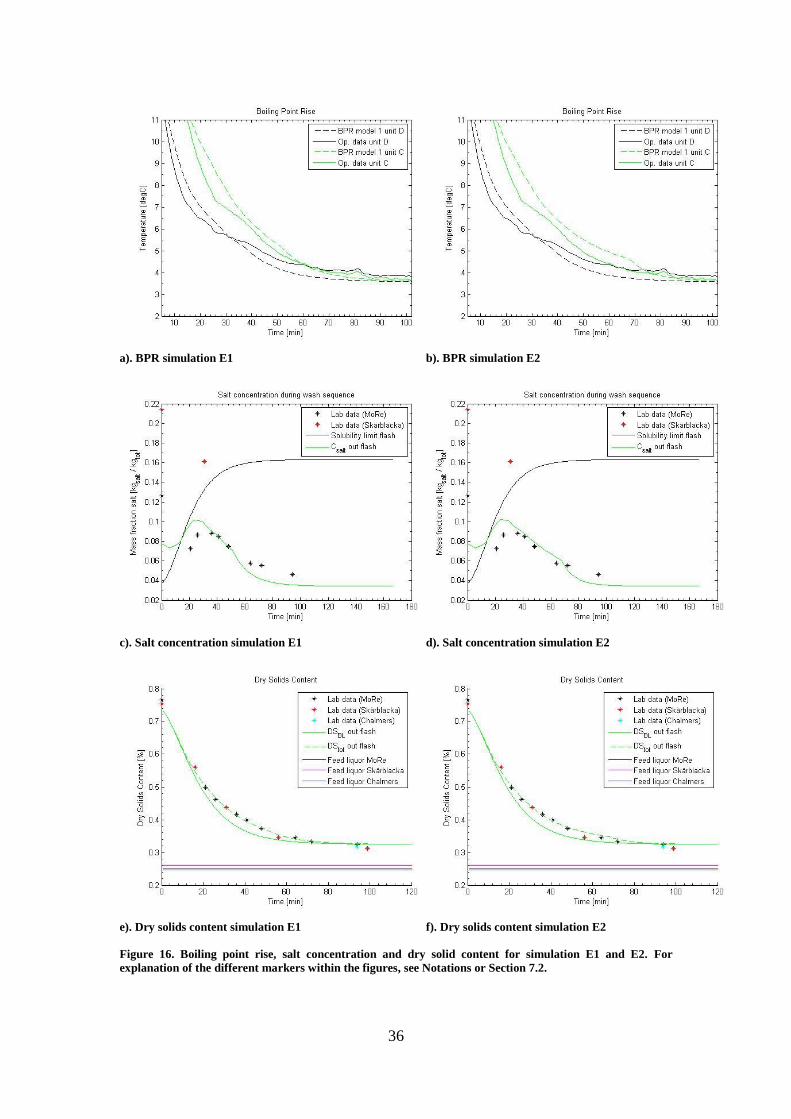
36

a). BPR simulation E1

b). BPR simulation E2

c). Salt concentration simulation E1

d). Salt concentration simulation E2

e). Dry solids content simulation E1

f). Dry solids content simulation E2

Figure 16. Boiling point rise, salt concentration and dry solid content for simulation E1 and E2. For

explanation of the different markers within the figures, see Notations or Section 7.2.

37

Comparing the BPR behaviour for the two simulations shows that the thicker layer of

scales applied to the bottom of unit 1C for simulation E2 causes in general less good

agreement with process data (Figure 16a and Figure 16b). On the other hand, studying

the figures illustrating salt concentration (Figure 16c and Figure 16d) indicates that

the agreement between wash model and lab data is better for simulation E2. Due to

the larger amount of scales simulation E2 give raise to longer dissolution time of salts,

and this improves the accordance with lab data. Finally, Figure 16e and Figure 16f

showing how the dry solids content of the liquor leaving the flash changes during the

wash procedure was evaluated. The increased layer of scales at the bottom of unit 1C

has not a large impact on DS, but a trend that the wash model DS overestimates lab

data after approximately 50 minutes of the wash has passed can be observed. This

indicates that the amount of scales at the bottom is too high. Another observation

made is that the difference between DSBL and DStot is larger for simulation E2 than

E1. This is a logical behaviour and occurs, as presented earlier, due to that the amount

of dissolved scales are higher.

In addition to the results shown in Figure 16 the deviation in heat transfer coefficient

was also evaluated. Due to equal scale distribution within unit 1D also the deviation

was identical and close to 16% for both simulation E1 and E2. For unit 1C only a

small difference in 𝑈-value for the two simulations was observed, 36.9% for

simulation E1 compared to 36.7% for simulation E2.

The results of simulations E1 and E2 illustrate the difficulty to achieve good

agreement between wash model and process data both concerning BPR and heat

transfer coefficient. To decrease the deviation in 𝑈-value, more scales are needed on

the tube walls but this will also lead to less good agreement in BPR. Comparison of

simulation E1 and E2 also indicates that the heat transfer coefficient has very low

sensitivity towards large variation in scale thickness if the changes only occur at a

small part of the tube.

39

8 Summarizing Discussion

The possibility to use the cleaning model to predict the scale distribution in an

industrial evaporator is found to be complicated due to the complexity of the studied

system. The model contains many input parameters that can be varied and each

parameter influences the results in different ways.

It is found that the BPR for the second unit is highly affected by the scale distribution

in the previous unit. The accordance for the first unit at the end of the wash is

improved if the layer of scales at the bottom of the tubes is thick, but as a

consequence, this overestimates the second unit BPR from process data during the

whole wash procedure.

Analysis of the heat transfer coefficient indicates that there are almost twice as much

scales in the second unit. A contradiction is met when combining this argumentation

with BPR analysis. For the calculated overall heat transfer coefficient, the 𝑈-value, to

have good agreement with the value from process data it is necessary to increase the

scale thickness at a large area at higher sections of the tubes. But boiling point rise

comparison between cleaning model and process data indicates that the scale

thicknesses at the upper sections of the tubes are thin. The same indications are given

from evaluation of salt concentration. Any explanation to this contradiction between

BPR observations and 𝑈-value observations has not been found.

It is concluded that the overall heat transfer coefficient has very low sensitivity

towards large variation in scale thickness if the changes only occurs at a small part of

the tube, whilst BPR shows high sensitivity to any change in scale thickness.

Better agreement between the cleaning model and process data is obtained if the

steam flow is increased with a factor 1.4 compared to the values from the control

system. It is highly doubted that the margin of error for the sensors collecting steam

flow values is that large, but if the analysis is widen and the error is seen as a

cumulative term for the whole control system the results might appear more probable.

The accuracy of the analysed salt contents is questioned. The fluctuation is not

consistent and salts that depends on each other changes with different magnitude.

Also, the deviation between analyses performed at different laboratories is large.

Therefore, it is concluded that when comparing the cleaning model with process data

and lab results, higher reliability shall be asserted to dry solids content and BPR than

salt concentration.

41

9 Conclusions

In this thesis, a dynamic model simulating the cleaning procedure of two evaporator

units connected in series has been developed. One of the most important inputs to the

model is the scale distribution, which unfortunately is unknown. A method to predict

it using the combination of boiling point rise (BPR) and overall heat transfer

coefficient was found simple and reasonable. A full scale test was successfully

performed at BillerudKorsnäs mill in Skärblacka, and both liquor samples and data

from the control system was collected during one wash procedure.

BPR is proven to have high sensitivity towards changes in scale distribution and is

found to be the most robust parameter to effectively monitor trends during the wash

procedure. It is therefore concluded that observing the BPR is a good measure to

determine if the evaporator tubes are clean or not. However, dry solids content

analyses show higher accuracy and therefore better predict absolute values.

The washing process also showed to be influenced by the steam flow rate. Larger

steam flow implies larger evaporation rate and if it is desirable to have as short

cleaning time as possible, the evaporation rate should be low.

Results of the performed simulations revealed that the model predicts faster cleaning

than online process data and lab analysis. This is believed to be due to that the model

assumes the cleaning to be identical for all tubes within the evaporator. In reality the

scales could be differently distributed on the tubes and there could also be clusters of

scales between some of the tubes, which the model is not able to account for.

For the studied wash at Skärblacka, it was not possible to predict the most probable

scale distributions. The simulation results of BPR and heat transfer coefficient was not

consistent, distributions generating good fit in BPR gave rise to a large deviation

concerning heat transfer coefficient and vice versa. One possible explanation to this

could be as mentioned above that the model assumes identical cleaning procedure for

all tubes. Another could be low accuracy of the collected process data. A final

conclusion is therefore that it would have been desirable to collect additional process

data and liquor samples from other full scale wash experiments. Then the robustness

of the investigation could be improved and possible inaccuracies with the data from

the studied wash at Skärblacka would have been detected.

43

References

ADAMS, T. N. 1997. General Characteristics of Kraft Black Liquor recovery Boilers.

Kraft Recovery Boilers. New York: Tappi Press.

BACK, S. 2014. 900 väl satsade miljoner. SPCI/Svensk papperstidning, 9.

BROBERG, A. & ÅKESJÖ, A. 2012. Experimental investigation and modelling of

sodium scale dissolution rates in black liquor evaporators. Göteborg: Chalmers

University of Technology. (Master’s Thesis within the Department of Energy

and Environment, Division of Heat and Power Technology).

CLAY, D. T. 2008. Evaporator Fouling. Jacobs Engineering Group Inc.

DEMARTINI, N. & FREDERICK, W. J. 2008. Review of Sodium Salt Scaling in the

Liquid Streams of the Chemical Recovery Cycle of Kraft Pulp Mills.

ENERGIMYNDIGHETEN 2013. <Energiläget 2013.pdf>.

FREDERICK, J. 1997. Black Liquor Properties. Kraft Recovery Boilers. New York:

Tappi Press.

FREDERICK JR, W. J., SHI, B., EUHUS, D. D. & ROUSSEAU, R. W. 2004.

Crystallization and control of sodium salt scales in black liquor concentrators.

Tappi Journal, 3, 7-13.

GOURDON, M. 2009. Sodium Salt Scaling in Black Liquor Evaporators.

Göteborg: Chalmers University of Technology. (Dissertation within the

Department of Energy and Environment, Division of Heat and Power

Technology).

GULLICHSEN, J. & FOGELHOLM, C.-J. 1999. Chemical Pulping, Jyväskyla,

Finland, Gummerus Printing.

HAJIHA, H., TRAN, H., WEBSDALE, O., HOLIK, D. & DOWNING, B.

Multivariate analysis of variables affecting thermal performance of black

liquor evaporators. TAPPI Press - TAPPI Engineering, Pulping and

Environmental Conference 2009 - Innovations in Energy, Fiber and

Compliance, 2009. 2246-2284.

KARLSSON, E., GOURDON, M. & VAMLING, L. Modeling and Evaluation of

Evaporator Cleaning. 2014a Proceedings of the 2014 International Chemical

Recovery Conference. 234-247.

KARLSSON, E., GOURDON, M. & VAMLING, L. 2014b. Solid Dissolution into a

Vertical Falling Film under Industrial-like Conditions. Industrial &

Engineering Chemistry Research, 53, 9478-9487.

KASSBERG, M. 1994. Lutindunstning och biproducter, Markaryd, Skogsindustrins

Utbildning i Markaryd AB.

PETTERSON, M. & ÖHRMAN, K. 2013. Experimental investigation and modelling

of sodium scale dissolution with black liquor. Göteborg: Chalmers University

of Technology. (Master’s Thesis within the Department of Energy and

Environment, Division of Heat and Power Technology).

REDEBORN, M. 2014. Manager Recovery Area at Billerud Skärblacka AB (2014-

10-09) Interviewed by the author.

44

SCHMIDL, W. & FREDERICK, W. J. Current trends in evaporator fouling. In:

ANON, ed. Proceedings of the 1998 International Chemical Recovery

Conference. Part 1 (of 3), 1998 Norcross, GA, United States, Tampa, FL,

USA. TAPPI Press, 367-377.

SCHNABEL, G. & SCHÜNDER, E. U. 1980. Wärmeübergang von senkrechten

Wänden an nichtsiedende und siedende Rieselfilme. Verfahrenstechnik 14, 79-

83.

SHI, B. 2002. Crystallization of solutes that lead to scale formation in black liquor

evaporation. 3046933 Ph.D., Georgia Institute of Technology.

SKOGSINDUSTRIERNA. 2013. Energieffektivisering -Mål 4 [Online]. Available:

http://www.skogsindustrierna.org/branschen/hallbar-

utveckling/hallbarhetsmal/energieffektivisering [Accessed 3 September 2014].

SMITH, J. B. 2000. Sodium salt scaling in falling film black liquor evaporators.

(Ph.D, Thesis, Georgia Institute of Technology).

VALMET 2014a. Company exclusive web-based education: IMT for Engineers

(performed at 2014-09-29).

VALMET 2014b. Recieved from Valmet co-workers (2014-09-29 to 2014-1102)

Interviewed by the author,. Valmet AB.

WELTY, J. R., WICKS, C. E., WILSON, R. E. & RORRER, G. L. 2001.

Fundamentals of Momentum, Heat, and Mass Transfer, New York, John

Wiley & Sons, Inc.

WENNBERG, O. 1990. Sulfat- och sulfitlutar fysikaliska-kemiska egenskaper. STU

projektnr 88-03869. Fig 6. Kokpunktsförhöjningen avsatt mot molaliteten,

molalitet av Na,K.

VERRILL, C. L. & FREDERICK JR, W. J. Evaporator fouling 101 - Sodium salt

crystallization and soluble-scale fouling. 2005 TAPPI Engineering, Pulping,

Environmental Conference - Conference Proceedings, 2006.

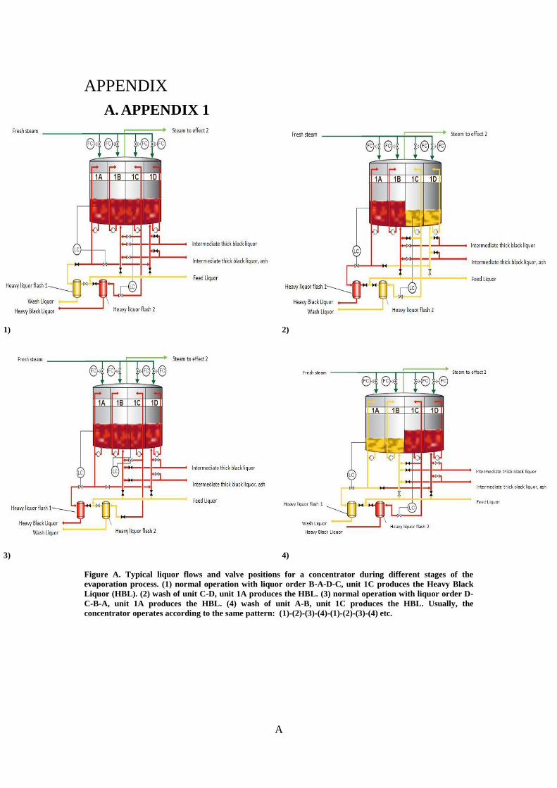
http://www.skogsindustrierna.org/branschen/hallbar-utveckling/hallbarhetsmal/energieffektivisering

http://www.skogsindustrierna.org/branschen/hallbar-utveckling/hallbarhetsmal/energieffektivisering

A

APPENDIX

A. APPENDIX 1

1)

2)

3)

4)

Figure A. Typical liquor flows and valve positions for a concentrator during different stages of the

evaporation process. (1) normal operation with liquor order B-A-D-C, unit 1C produces the Heavy Black

Liquor (HBL). (2) wash of unit C-D, unit 1A produces the HBL. (3) normal operation with liquor order D-

C-B-A, unit 1A produces the HBL. (4) wash of unit A-B, unit 1C produces the HBL. Usually, the

concentrator operates according to the same pattern: (1)-(2)-(3)-(4)-(1)-(2)-(3)-(4) etc.

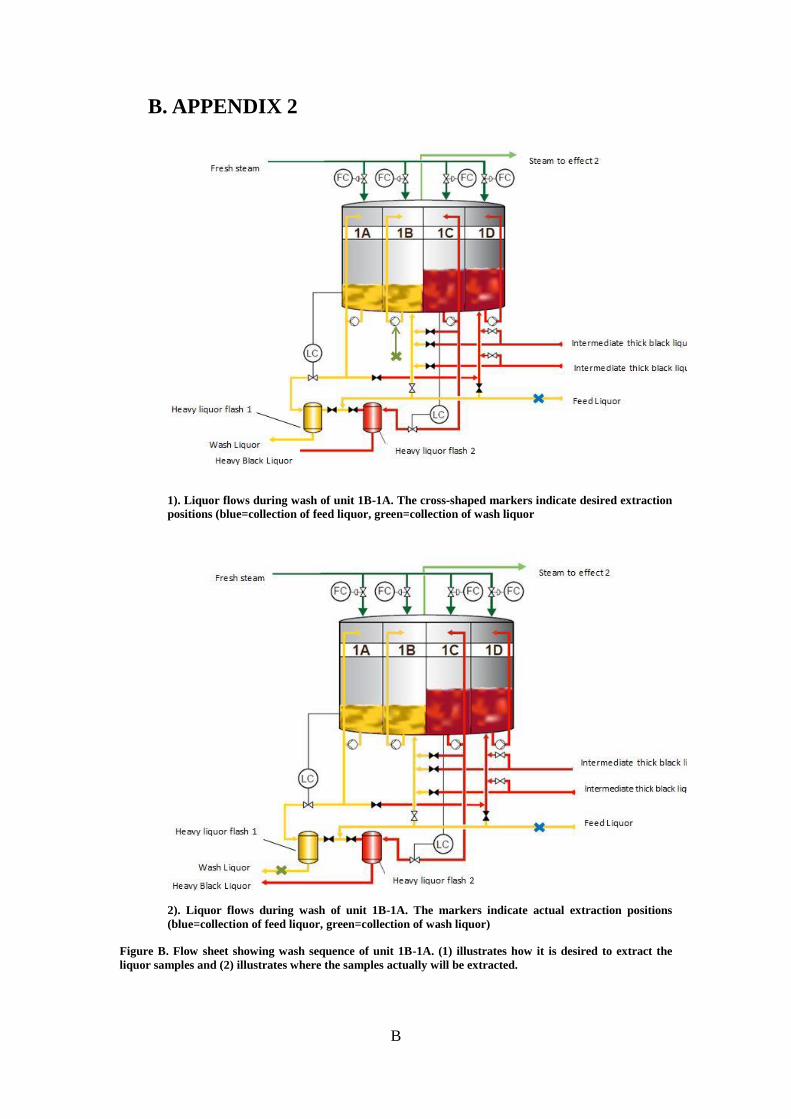
B

B. APPENDIX 2

1). Liquor flows during wash of unit 1B-1A. The cross-shaped markers indicate desired extraction

positions (blue=collection of feed liquor, green=collection of wash liquor

2). Liquor flows during wash of unit 1B-1A. The markers indicate actual extraction positions

(blue=collection of feed liquor, green=collection of wash liquor)

Figure B. Flow sheet showing wash sequence of unit 1B-1A. (1) illustrates how it is desired to extract the

liquor samples and (2) illustrates where the samples actually will be extracted.

C

C. APPENDIX 3

From laboratory analysis the amount of sulphate and carbonate, 𝑚𝑆𝑂4and 𝑚𝐶𝑂3

, was

obtained.

It is also known that the scales consist of sodium sulphate and sodium carbonate,

which have following chemical formulas:

Sodium sulphate=𝑁𝑎2𝑆𝑂4

Sodium carbonate=𝑁𝑎2𝐶𝑂3

The molar mass for the different substances was defined according to:

𝑀𝑁𝑎 = 22.99𝑔

𝑚𝑜𝑙𝑒

𝑀𝑆𝑂4= 32.06 + 4 ∙ 16 = 96.06

𝑔

𝑚𝑜𝑙𝑒

𝑀𝐶𝑂3= 12.01 + 3 ∙ 16 = 60.01

𝑔

𝑚𝑜𝑙𝑒

The amount of moles for sulphate and carbonate was determined using the molar mass

together with the laboratory results:

𝑛𝑆𝑂4=

𝑚𝑆𝑂4

𝑀𝑆𝑂4

𝑚𝑜𝑙𝑒

𝑛𝐶𝑂3=

𝑚𝐶𝑂3

𝑀𝐶𝑂3

𝑚𝑜𝑙𝑒

From the molar ratio of the scaling salts, the amounts of mole sodium within the

scales were calculated:

𝑛𝑁𝑎,𝑠𝑐𝑎𝑙𝑒 = (2 ∙ 𝑛𝑆𝑂4+ 2 ∙ 𝑛𝐶𝑂3

)𝑚𝑜𝑙𝑒

Then, the amount of sodium associated to the scales could be calculated:

𝑚𝑁𝑎,𝑠𝑐𝑎𝑙𝑒 = 𝑛𝑁𝑎,𝑠𝑐𝑎𝑙𝑒 ∙ 𝑀𝑁𝑎 [𝑔/𝑘𝑔𝐷𝑆],

The total amount of scaling salt was the determined:

𝑚𝑠𝑐𝑎𝑙𝑒 = 𝑚𝑆𝑂4+ 𝑚𝐶𝑂3

+ 𝑚𝑁𝑎,𝑠𝑐𝑎𝑙𝑒

Since the laboratory analysis were given as [𝑔/𝑘𝑔𝐷𝑆], the analysed dry solids content

were used to obtain desired unit [𝑘𝑔/𝑘𝑔𝑡𝑜𝑡]

𝐶 =𝑚𝑠𝑐𝑎𝑙𝑒 ∗

𝐷𝑆100

1000 [𝑘𝑔𝑠𝑎𝑙𝑡/𝑘𝑔𝑡𝑜𝑡]

D

When the values from the laboratory analysis were inserted into the equation

calculating the salt concentration, following results were obtained.

Table A. Salt concentration calculated from the analyse results from the different laboratories. All values

are given in the unit [𝒌𝒈/𝒌𝒈𝒕𝒐𝒕].

Cum. time MoRe Research Skärblacka

0 0.1263 0.2140

16 - -

21 0.0724 -

26 0.0864 -

31 - 0.1614

36 0.0879 -

41 0.0845 -

48 0.0745 -

56 -

64 0.0579 -

72 0.0554 -

94 0.0461 -

99 - -

In the figures showing salt concentration, the values from analyses performed by

MoRe Research are illustrated by black dots and the ones from Skärblacka by red

dots.

E

D. APPENDIX 4

1). U-value development for unit 1D before and during performed wash sequence. Green arrow indicates when the tubes are

considered clean and red arrow when the wash was initiated, i.e. when the tubes are fouled.

2) U-value development for unit 1C before and during performed wash sequence. Green arrow indicates when the tubes are

considered clean and red arrow when the wash was initiated, i.e. when the tubes are fouled.

Figure C. U-value development for concentrator unit 1D (1) and unit 1C (2) before and during performed

wash sequence.

0

500

1000

1500

2000

2500

2014-10-05 00:00 2014-10-06 00:00 2014-10-07 00:00 2014-10-08 00:00 2014-10-09 00:00

[W/(m2,K)]

U-value 1D

0

200

400

600

800

1000

1200

1400

2014-10-05 00:00 2014-10-06 00:00 2014-10-07 00:00 2014-10-08 00:00 2014-10-09 00:00

[W/(m2,K)]

U-value 1C

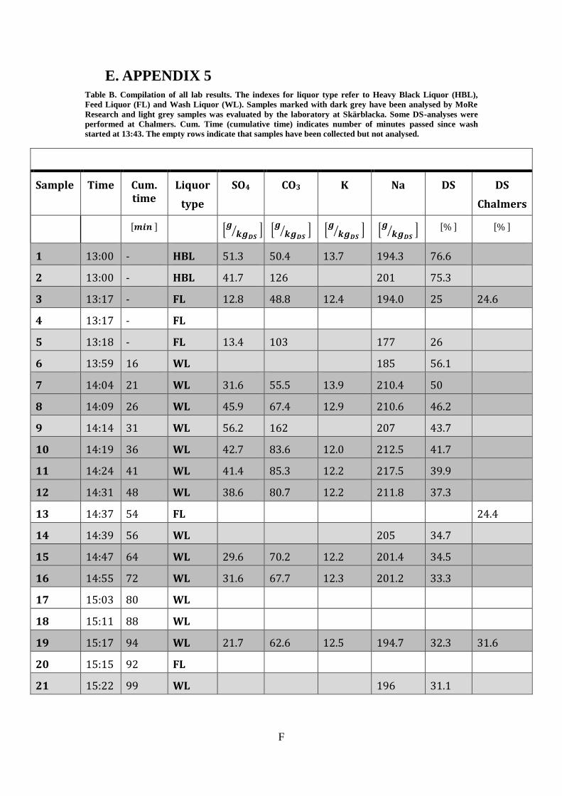
F

E. APPENDIX 5

Table B. Compilation of all lab results. The indexes for liquor type refer to Heavy Black Liquor (HBL),

Feed Liquor (FL) and Wash Liquor (WL). Samples marked with dark grey have been analysed by MoRe

Research and light grey samples was evaluated by the laboratory at Skärblacka. Some DS-analyses were

performed at Chalmers. Cum. Time (cumulative time) indicates number of minutes passed since wash

started at 13:43. The empty rows indicate that samples have been collected but not analysed.

Sample Time Cum. time

Liquor

type

SO4 CO3 K Na DS DS

Chalmers

[𝒎𝒊𝒏 ] [𝒈



⁄ ] [𝒈



⁄ ] [% ] [% ]

1 13:00 - HBL 51.3 50.4 13.7 194.3 76.6

2 13:00 - HBL 41.7 126 201 75.3

3 13:17 - FL 12.8 48.8 12.4 194.0 25 24.6

4 13:17 - FL

5 13:18 - FL 13.4 103 177 26

6 13:59 16 WL 185 56.1

7 14:04 21 WL 31.6 55.5 13.9 210.4 50

8 14:09 26 WL 45.9 67.4 12.9 210.6 46.2

9 14:14 31 WL 56.2 162 207 43.7

10 14:19 36 WL 42.7 83.6 12.0 212.5 41.7

11 14:24 41 WL 41.4 85.3 12.2 217.5 39.9

12 14:31 48 WL 38.6 80.7 12.2 211.8 37.3

13 14:37 54 FL 24.4

14 14:39 56 WL 205 34.7

15 14:47 64 WL 29.6 70.2 12.2 201.4 34.5

16 14:55 72 WL 31.6 67.7 12.3 201.2 33.3

17 15:03 80 WL

18 15:11 88 WL

19 15:17 94 WL 21.7 62.6 12.5 194.7 32.3 31.6

20 15:15 92 FL

21 15:22 99 WL 196 31.1