modelling of a simple continuous neutralisation...

Modelling of a simple continuous

neutralisation reactor

Serge Zihlmann

ThirdWay

February 23, 2015

Modelling of a neutralisation reactor

Foreword

When I was browsing the web for a decent and intuitive model of a neutralisation reactor,I could not nd the appropriate theorethical descripton nor model les for download. Atthat time I started to develop an own model including its implementation in a Simulationsoftware. Quickly, this ended up in a rather extensive project.

The theory developed and the models used are described in this little script in twodierent ways: One more intuitively and the other more academic. The models can ofcourse be downloaded read to use.

S. Zihlmann February 23, 2015 Page 1 of 18


1 Introduction and Modelling

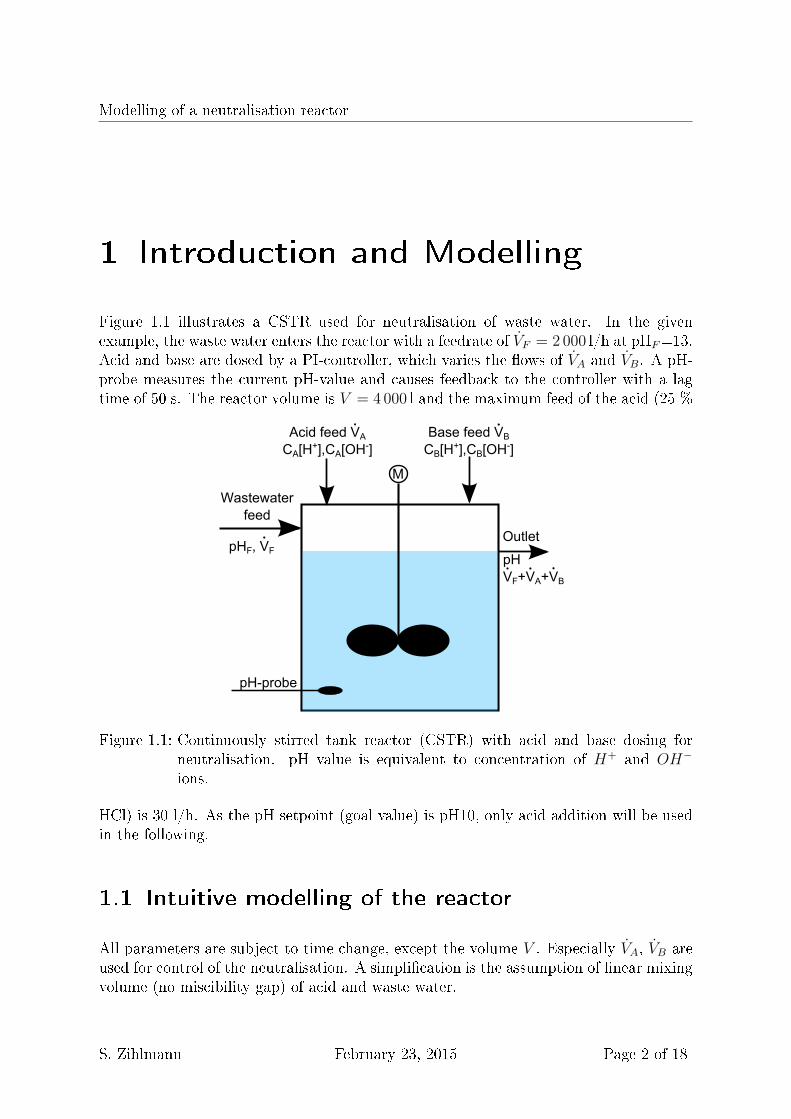
Figure 1.1 illustrates a CSTR used for neutralisation of waste water. In the givenexample, the waste water enters the reactor with a feedrate of VF = 2 000 l/h at pHF=13.Acid and base are dosed by a PI-controller, which varies the ows of VA and VB. A pH-probe measures the current pH-value and causes feedback to the controller with a lagtime of 50 s. The reactor volume is V = 4 000 l and the maximum feed of the acid (25 %

Wastewaterfeed

M

pHF, VF

Acid feed VA

CA[H+],CA[OH-]Base feed VB

CB[H+],CB[OH-]

pHVF+VA+VB

Outlet

pH-probe

Figure 1.1: Continuously stirred tank reactor (CSTR) with acid and base dosing forneutralisation. pH value is equivalent to concentration of H+ and OH−

ions.

HCl) is 30 l/h. As the pH setpoint (goal value) is pH10, only acid addition will be usedin the following.

1.1 Intuitive modelling of the reactor

All parameters are subject to time change, except the volume V . Especially VA, VB areused for control of the neutralisation. A simplication is the assumption of linear mixingvolume (no miscibility gap) of acid and waste water.



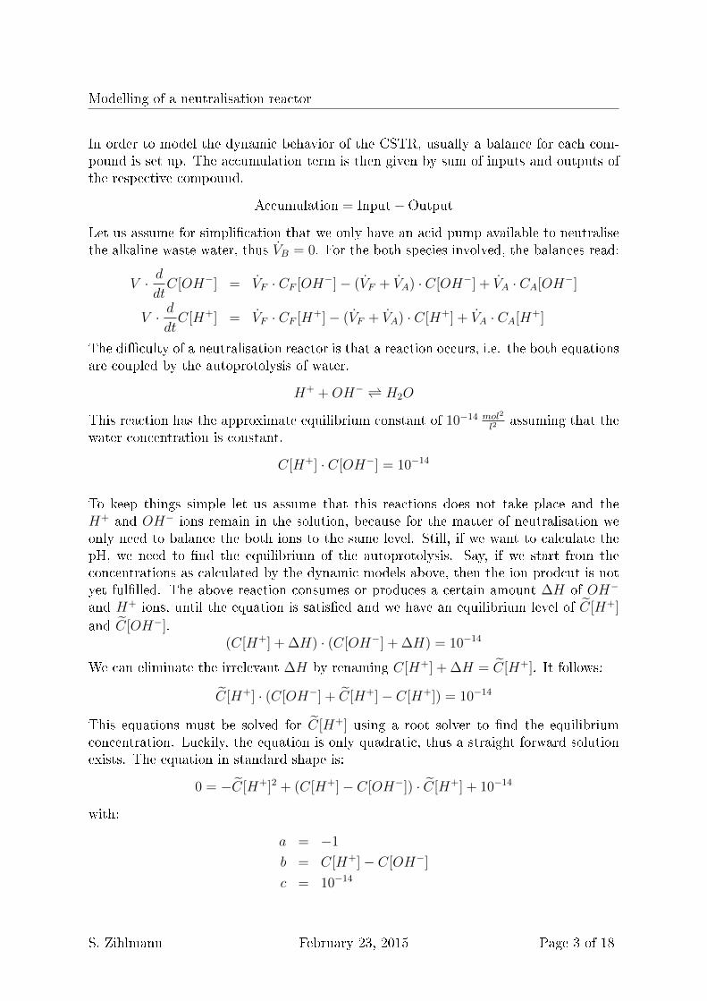
In order to model the dynamic behavior of the CSTR, usually a balance for each com-pound is set up. The accumulation term is then given by sum of inputs and outputs ofthe respective compound.

Accumulation = Input−Output

Let us assume for simplication that we only have an acid pump available to neutralisethe alkaline waste water, thus VB = 0. For the both species involved, the balances read:

V · ddtC[OH−] = VF · CF [OH−]− (VF + VA) · C[OH−] + VA · CA[OH−]

V · ddtC[H+] = VF · CF [H+]− (VF + VA) · C[H+] + VA · CA[H+]

The diculty of a neutralisation reactor is that a reaction occurs, i.e. the both equationsare coupled by the autoprotolysis of water.

H+ + OH− H2O

This reaction has the approximate equilibrium constant of 10−14 mol2

l2assuming that the

water concentration is constant.

C[H+] · C[OH−] = 10−14

To keep things simple let us assume that this reactions does not take place and theH+ and OH− ions remain in the solution, because for the matter of neutralisation weonly need to balance the both ions to the same level. Still, if we want to calculate thepH, we need to nd the equilibrium of the autoprotolysis. Say, if we start from theconcentrations as calculated by the dynamic models above, then the ion prodcut is notyet fullled. The above reaction consumes or produces a certain amount ∆H of OH−

and H+ ions, until the equation is satised and we have an equilibrium level of C[H+]

and C[OH−].(C[H+] + ∆H) · (C[OH−] + ∆H) = 10−14

We can eliminate the irrelevant ∆H by renaming C[H+] + ∆H = C[H+]. It follows:

C[H+] · (C[OH−] + C[H+]− C[H+]) = 10−14

This equations must be solved for C[H+] using a root solver to nd the equilibriumconcentration. Luckily, the equation is only quadratic, thus a straight forward solutionexists. The equation in standard shape is:

0 = −C[H+]2 + (C[H+]− C[OH−]) · C[H+] + 10−14

with:

a = −1

b = C[H+]− C[OH−]

c = 10−14



The solution is:

C[H+]1,2 =−b±

√b2 − 4ac

2a

While only one of the two solutions retrieves a positive concentration. It can further besimplied to depend only on the input concentration of H+ and OH− ions:

C[H+] =1

2

(b +√b2 + 4 · 10−14

)And the pH value will read:

pH = −log10(C[H+])

We see that the dierence b of the ion concentration plays a central role to the solutionof the problem. Let's try to combine the two dierential equations by subtracting therst from the second.

V · ddt

(C[H+]− C[OH−]) =

VF · (CF [H+]−CF [OH−])− (VF + VA) · (C[H+]−C[OH−]) + VA · (CA[H+]−CA[OH−])

We can identify some terms by b, bF and bA:

V · ddtb = VF · bF − (VF + VA) · b + VA · bA

The neutralisation problem can now be solved by one simple ODE. Note: For the mod-elling of base addition, the term VB · bB must be added to the right side.

1.1.1 Dynamic behavior

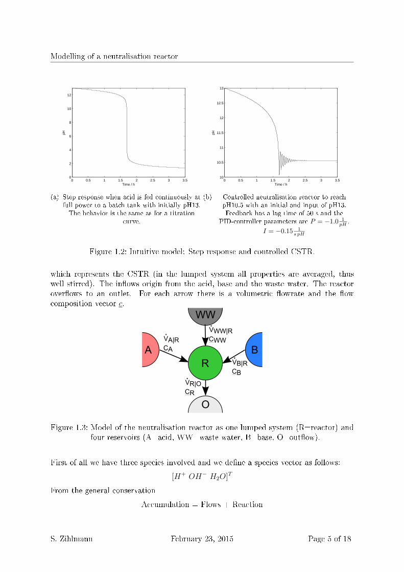
The model was implemented in Simulink (see Appendix) and the dynamic behaviorin terms of step response and PI-controlled CSTR are shown in gure 1.2. The stepresponse when suddenly acid is fed to the reactor with otherwise constant inow, can beinterpreted as titration curve. The controlled plant is quite sensitive to oscillation dueto the lag time of the pH-electrode (here 50 s) and the high nonlinearity, for which thePID's are not well designed.

1.2 Second approach

One might ask whether there is a more sophisticate approach to the modelling partin contrast to the previous rather intuitive model. Of course there is a more strict,mathemathical way but the intuitive has its advantage that the user understands theprocess behind well. To proceed with the model in the academic way, I propose amore simplied model structure (gure 1.3) which contstitutes of one lumped system



0 0.5 1 1.5 2 2.5 3 3.50

2

4

6

8

10

12

Time / h

pH

(a) Step response when acid is fed continuously atfull power to a batch tank with initially pH13.The behavior is the same as for a titration

curve.

0 0.5 1 1.5 2 2.5 3 3.510

10.5

11

11.5

12

12.5

13

Time / h

pH

(b) Controlled neutralisation reactor to reachpH10.5 with an initial and input of pH13.Feedback has a lag time of 50 s and the

PID-controller parameters are P = −1.0 1pH ,

I = −0.15 1s pH

Figure 1.2: Intuitive model: Step response and controlled CSTR.

which represents the CSTR (in the lumped system all properties are averaged, thuswell stirred). The inows origin from the acid, base and the waste water. The reactoroverows to an outlet. For each arrow there is a volumetric owrate and the owcomposition vector c.

RA

WW

B

O

VR|OCR

VB|RCB

VA|RCA

VWW|RCWW

Figure 1.3: Model of the neutralisation reactor as one lumped system (R=reactor) andfour reservoirs (A=acid, WW=waste water, B=base, O=outow).

First of all we have three species involved and we dene a species vector as follows:

[H+ OH− H2O]T

From the general conservation

Accumulation = Flows + Reaction



There follows directly the equation in matrix notation:

nR = F n + nr

Where nR is the total change in moles of each compound in the reactor, n is the molarow of each compound and in each stream, F represents the direction matrix of the ows(in or out) and is only a selector matrix, nr represents the production/consumption byreaction (= index r) of each compound within the reactor. More specic, the ow vectorconsists of (omitting the base ow)

n =

nA|RnWW |RnR|O

And the ow selector matrix:

F =

1 0 00 1 00 0 1

1 0 00 1 00 0 1

−1 0 00 −1 00 0 −1

= [ 1 1 −1 ]⊗ I

The notation is very ecient using the kronecker product ⊗. The molar ow in eachstream is simply nx|y = Vx|y · cx for an exemplary ow from tank x to y. The input

ows VA|R and VWW |R are well dened as well as their composition cA, cWW . Theoutlet ow must be obtained from an assumption. Here it is, that the volume duringmixing of the two streams remains constant and the reactor has constant volume, thusVR|O = VA|R + VWW |R. The composition of the outlet cR ow changes with time andmust be obtained from the dynamic model cR = V −1nR where V is the volume of thereactor.

1.2.1 Including the reaction

The reaction term nr mentioned in the last section is represented by the reaction sto-chiometry matrix N and some extent of reaction n.

nr = NT n

For the autodissociation of the water

H2Okf

kb

H+ + OH−

the reaction stochiometri matrix reads

N =

[1 1 −1−1 −1 1

]forwardbackward



for the forward and backward reaction. The reaction extent is formulated by the reactionrate law

nr = NT VKr g(cr)

where V is the reactor volume, Kr contains the reaction rate constants and g(cr) is the

formulation of the rate law. Joined in one equation:

nR = F n + NT VKr g(cr)

The central assumption for the further procedure is that the autoprotolysis reactionof the water is very fast. In other words, the reaction reaches always the equilibrium.Therefore we will eliminate the reaction term by nding the left nullspace Ω of NT andit is

Ω =

[1 −1 01 0 1

]Of course there exists an innite amount of possible nullspaces, it is selected in thatway that the equations used during root solving become nice. By multiplying the wholeequation with the left null space, we eliminate the reaction terms.

Ω nR = ΩF n + ΩNT VKr g(cr)

Ω nR = ΩF n

After the nullspace transformation we can identify a new state zR = ΩnR

zR = ΩF n

Now the dynamic model is nished and simply the ODE for the state zR has to besolved. n is dened by the input variables (acid ow, waste water ow) and the reactorcomposition (feedback). That requires the reconstruction of the reactor composition cRfrom the state zR. That involves solving the roots of the equation

0 = zR −ΩnR = zR −ΩV cR

In this case we need to solve for three dimensions in the space of cR but the aboveexpression returns only two equations. Thus we need another condition and it originatesfrom the reaction term, more precisely, the equilbrium relation:

0 = NT VKr g(cr) (1.1)

0 =

1 −11 −1−1 1

V

[kf 00 kb

] [cH2O

cH+ · cOH−

](1.2)

0 = V

kf · cH2O − kb · cH+ · cOH−

kf · cH2O − kb · cH+ · cOH−

−kf · cH2O + kb · cH+ · cOH−

(1.3)

(1.4)



The three equations are equal and result in

kbkf

=cH2O

cH+ · cOH−

The concentration of the water is assumed constant and the equilibrium constant equalto 1014 as generally for the water dissoziation.

k1 =1

cH+ · cOH−= 1014

Thus the third required equation to reconstruct the composition cR from the state zR is

0 = k1 −1

cH+ · cOH−

Finally we have to fulll all three equations:

0 =

[zR −ΩV cRk1 − 1

cH+ ·cOH−

]This can be solved for cR by a numerical root solver, but in this simple case explicitexpressions are available. In detailed formulation this reads:

0 =

z1 − V (cH+ − cOH−)z2 − V (cH+ + cH2O)

k1 − 1cH+ ·cOH−

After solving this system one obtains:

cH+ =1

2

(z1V

+

√(z1V

)2+

4

k1

)(1.5)

cOH− =1

k1cH+

(1.6)

cH2O =z2V− cH+ (1.7)

Now the modelling is complete and the structure can be implemented into a numericalsoftware. The concentration vector for each input ow must be obtained from the pH oracid/base concentration. For the water always a constant concentration of 55.6 mol/L isassumed. One central dierence of this model to the intuitive one is that also the wateris balanced.

1.2.2 Dynamic behavior

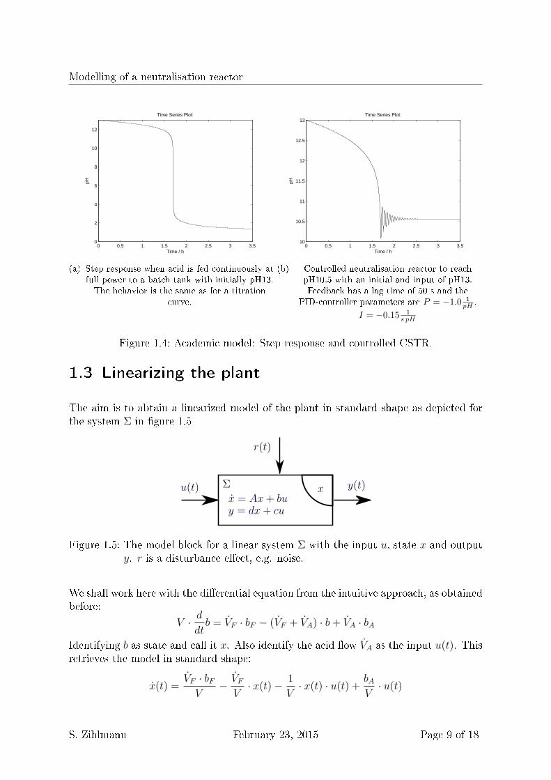
In gure 1.4 the results of the dynamic Simulink model for the academic approach areshown. The results is equal to the intuitive approach.



0 0.5 1 1.5 2 2.5 3 3.50

2

4

6

8

10

12

Time / h

pH

Time Series Plot:

(a) Step response when acid is fed continuously atfull power to a batch tank with initially pH13.The behavior is the same as for a titration

curve.

0 0.5 1 1.5 2 2.5 3 3.510

10.5

11

11.5

12

12.5

13

Time / h

pH

Time Series Plot:

(b) Controlled neutralisation reactor to reachpH10.5 with an initial and input of pH13.Feedback has a lag time of 50 s and the

PID-controller parameters are P = −1.0 1pH ,

I = −0.15 1s pH

Figure 1.4: Academic model: Step response and controlled CSTR.

1.3 Linearizing the plant

The aim is to abtain a linearized model of the plant in standard shape as depicted forthe system Σ in gure 1.5

xx = Ax + buy = dx + cu

u(t) y(t)

r(t)

Σ

Figure 1.5: The model block for a linear system Σ with the input u, state x and outputy. r is a disturbance eect, e.g. noise.

We shall work here with the dierential equation from the intuitive approach, as obtainedbefore:

V · ddtb = VF · bF − (VF + VA) · b + VA · bA

Identifying b as state and call it x. Also identify the acid ow VA as the input u(t). Thisretrieves the model in standard shape:

x(t) =VF · bF

V− VF

V· x(t)− 1

V· x(t) · u(t) +

bAV· u(t)



The output of the plant is not b but the pH value. Therefore we needed the root solver:

C[H+] =1

2

(b +√b2 + 4 · 10−14

)and thus

pH = −log10(

1

2

(b +√b2 + 4 · 10−14

))In standard form, where pH is the output y(t) and b again the state x(t):

y(t) = −log10(

1

2

(x(t) +

√x2(t) + 4 · 10−14

))Thus we have the complete non linear model in standard shape: x(t) = VF ·bF

V− VF

V· x(t)− 1

V· x(t) · u(t) + bA

V· u(t) = f (x(t), u(t))

y(t) = −log10(

12

(x(t) +

√x2(t) + 4 · 10−14

))= g (x(t), u(t))

The linearization will bring the model into the shape:[

x(t) = Ax(t) + b u(t)y(t) = c x(t) + d u(t)

]While A, b, c and d are matrices in general, but here simple constants. The linearizationis done around the equilibrium point with x = xe and u = ue. In this equilibrium pointwe have:

0!

= x(t) =VF · bF

V− VF

V· xe− 1

V· xe · ue +

bAV· ue

Usually for this equilibrium point the plants steady state point without interactions ischosen (this would be in our case that the reactor has the same composition as the inletow). Because the model is highly non linear, this would not be a good choice sincewe want to control the pH in detail around pH10. Thus we select pH10 as linearizationpoint and have to search for the appropriate ue. b is readily calculated from the pH:

be =C2[H+]− 10−14

C[H+]=

10−2pH − 10−14

10−pH= 10−pH − 10pH−14

and thusxe = be = 10−10 − 10−4 = 10−4(10−6 − 1) ≈ −10−4

Now we have to nd the acid feed ue to reach steady pH10 (xe). Reformulation of theequation above:

ue = VFxe− bFbA − xe



The constants are then calculated:

A = ∂f∂x

∣∣u=ue

x=xe= − VF

V− 1

V· u(t)

∣∣∣u=ue

x=xe= − VF+ue

V

b = ∂f∂u

∣∣u=ue

x=xe= − 1

V· x(t) + bA

V

∣∣u=ue

x=xe= bA−xe

V

c = ∂g∂x

∣∣u=ue

x=xe= − 1

ln(10)√

x2(t)+4·10−14

∣∣∣∣u=ue

x=xe

= − 1ln(10)

√xe2+4·10−14

d = ∂g∂u

∣∣u=ue

x=xe= 0

The factor d appears to be zero, because the acid feed has no instantaneous eect ontothe pH value.

1.3.1 Dynamic behavior and linearization error

As the model is linearized around pH11, it is not a good idea to start the control atpH13 due to the high non-linearity. For this reason, two scenarios are compared here:

Control from pH12 to pH11 (strong disturbance)

Control from pH11.1 to pH11 (slight disturbance)

Each scenario is compared for the controlled linearized and full model (as from intuitiveapproach). Th results are depicted in gure 1.6. What is obvious is that the linearizedmodel starts at the wrong pH due to linearization error. This error becomes much lesswhen the starting point is pH11.1. For the big step in control variable, the dierencebetween the control characteristic of the full/linearrized model is quite large, whilstat a small step the error is negligible (less linearization error). As a consequence, themodeling with this linear model is only appropriate if the pH does not vary much fromthe setpoint (e.g. when keeping the level constant under disturbance).s

1.4 Transfer function

The transfer function represents the dynamic input/output behavior. The transfer func-tion in the laplace domain can not readily be calculated for the full model, as x and yoccur in a multiplication (which leads to a convolution in the laplace domain). Anyhow,it can be obtained quickly from the linearized model:[

x(t) = Ax(t) + b u(t)y(t) = c x(t) + d u(t)

]



0 0.2 0.4 0.6 0.8 110

10.2

10.4

10.6

10.8

11

11.2

11.4

11.6

11.8

12

Time / h

pH

Full modelLinearized

(a) Control from pH12 to pH11.

0 0.2 0.4 0.6 0.8 110.9

10.92

10.94

10.96

10.98

11

11.02

11.04

11.06

11.08

11.1

Time / h

pH

Full modelLinearized

(b) Control from pH11.1 to pH11.

Figure 1.6: Response of a controlled neutralisation CSTR for dierent starting/aim pH-values. Each plot shows the response of the full model compared to thelinearized plant. Parameters of the controller are the same as before (feed-back lag 50 s, P = −1.0 1

pH, I = −0.15 1

s pH

After a laplace transformation one obtains[x(s) · s = Ax(s) + b u(s)y(s) = c x(s) + d u(s)

]because A, b, c and d are simple constants. After algebraic operations:

x(s) =b · u(s)

s− A

Then

y(s) =

[c · bs− A

+ d

]u(s)

And the transfer function:

G(s) =y(s)

u(s)=

c · bs− A

+ d

Although derived here, this section is more for info than practical use.


2 Choosing a PID controller

2.1 Back-linearization

One might state that it is a good idea to `re-linearize' the plant, thus to take the outputpH value and calculate it back to the concentration of H+ ions. Also the setpoint shallbe given as a concentration of H+. The control would then be linear, anyhow across hugemagnitudes. The problem is then, that the chosen PID constants are only valid for aspecic case and nding parameters for a wide range of application would be impossible.E.g. switching the setpoint from pH11 to pH10 would make the control parametersuseless. Figure 2.1 contains three examples for illustration. The basic problem with this

0 0.5 1 1.5 2 2.5 3 3.510

10.5

11

11.5

12

12.5

13

Time / h

pH

(a) Control from pH13 to pH10.5.

0 0.5 1 1.5 2 2.5 3 3.510

10.5

11

11.5

12

12.5

13

Time / h

pH

(b) Control from pH13 to pH10.

0 0.5 1 1.5 2 2.5 3 3.510

10.5

11

11.5

12

12.5

13

Time / h

pH

(c) Control from pH13 to pH11.

Figure 2.1: Response of a controlled neutralisation CSTR with back-linearization fordierent set points of pH. The starting value is always pH13. One set of PIDparameters is not appropriate for all cases (optimized for case a) ). Feedbacklag 50 s, P = 2 · 1010 1

pH, I = 6 · 109 1

s pH.

approach is, that the overshoot (e.g. in example b) ) appears huge in the logarithmicdomain but is not in the linear (controlled) one. Keeping this logarithmic behavior inmind, the reverse case, when controllong from pH10, pH11 or pH12 to pH13 looks wellfor all cases.

It would be good to have some anti-windup1 in the real plant.

1The integral term gets windup very quickly (especially in this logarithmic domain), thus it accumu-lates an output that is larger than the maximal value for the regulation variable.

13

3 Appendix

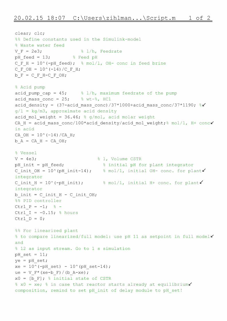
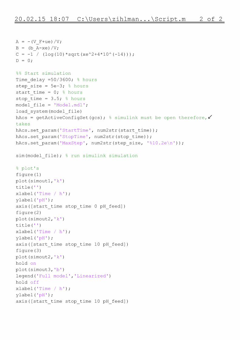
In gures 3.1 3.2 3.3 & 3.4 the models inplemented in Simulink for the intuitive model,its substructures and the linearized model are depicted. The last two pages containthe Matlab code to execute the models. All complete les can also be downloadedfrom http://www.thirdway.ch/En/projects/neutralisation_modeling (or thirdway.ch ->projects -> Neutralisation modeling). The Simulink models and code for the academicapproach are not shown here, but can be downloaded from the same place.

14


Controlled(linearized(plant

Controlled(neutralisation(plant

Acid(pumpset(point

Reactor(pH

Step(response(of(the(neutralisation

10.5

pH(setpoint Scope2

PID4s3

PI(Controller

TransportDelay

1

Acid(pumpsetpoint

Scope1

In1 Out1

CSTRneutralisation

reactor

In1 Out1

CSTRneutralisation

reactor1simout2

To(Workspace

pH_set

pH(setpoint1

PID4s3

PI(Controller1 Scope4

TransportDelay1

simout3

To(Workspace1

In1 Out1

Linearized(CSTR

simout1

To(Workspace2

Figure 3.1: Overview of the Simulink block structure for the intuitive approach. Stepresponse, controlled plant and controlled linearized plant.



Acid1feedrateV_A

Setpoint1acid1pump

b

b

Model1of1the1neutralisation1CSTR.1One1balance1for1each1of1H41and1OH-.

1

In1

1

Out1

-C-

Acid1pump1capacity 1/V

Gain2V_F

Feedrate

1sxo

integrator

Product2

b_A

CA_H

Product3Product4

b_init

b_init

Saturation

In1 Out1

Get1pH

b_F

b_FProduct1

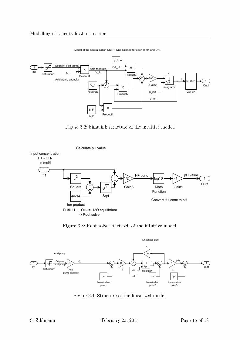
Figure 3.2: Simulink structure of the intuitive model.

CalculateGpHGvalue

InputGconcentrationH+G-GOH-inGmol/l

pHGvalue

FulfillGH+G+GOH-G=GH2OGequilibrium->GRootGsolver

ConvertGH+GconcGtoGpH

H+Gconc-1

Gain1

log10

MathFunction

1/2

Gain3

u2

Square u

Sqrt4e-14

IonGproduct

1

In11

Out1

Figure 3.3: Root solver `Get pH' of the intuitive model.

Setpointacid3pump

xu(t) y(t)

Acid3pump

Linearized3plant

Saturation1

-K-

Acidpump3capacity

1sxo

integratorx0

init

A

A

C

C

B

B

xe

linearizationpoint2

ye

linearizationpoint3

ue

linearizationpoint1

1

In1

1

Out1

Figure 3.4: Structure of the linearized model.


modelling of a simple continuous neutralisation...

Documents