modelling neuronal excitation: the hodgkin-huxley...

Modelling Neuronal Excitation: The

Hodgkin-Huxley Model

Thierry Mondeel

July 13, 2012

Contents

1 A short introduction to the biology of neurons 41.1 Neurons 51.2 The cell membrane and ion channels 6

1.2.1 The electrochemical gradient: Why does charge move? 71.2.2 The key ions: potassium and sodium . . . . . . . . . . 8

1.3 The action potential 101.3.1 The underlying currents . . . . . . . . . . . . . . . . . 10

2 Preliminary work: Membranes, channels and gradients 122.1 Single-compartment models 122.2 Capacitance and resistance 132.3 The membrane potential 132.4 The Nernst potential 14

2.4.1 The sodium and potassium equilibrium potentials . . 142.4.2 Ion pumps . . . . . . . . . . . . . . . . . . . . . . . . . 142.4.3 The Goldman equation . . . . . . . . . . . . . . . . . 15

2.5 The form of Iion 152.6 The Hodgkin-Huxley gate model 16

2.6.1 Persistent conductance . . . . . . . . . . . . . . . . . . 172.6.2 Transient conductance . . . . . . . . . . . . . . . . . . 18

3 The Hodgkin-Huxley model 203.1 The work of Hodgkin and Huxley in perspective 203.2 Combining the preliminary work 21

3.2.1 The sodium and potassium conductances . . . . . . . 223.2.2 Summary of the equations . . . . . . . . . . . . . . . . 23

3.3 The dynamics 24

4 The Fitzhugh-Nagumo model 264.1 History and perspective 264.2 The fast-slow simplification of the HH model 274.3 The fast-slow phase plane 284.4 The FitzHugh-Nagumo equations 29

1

0.0 2

5 Summary 345.1 Review 345.2 Futher studies 35

6 Sources 37

Preface

This is a bachelor thesis about mathematical models that describe the de-velopment and propagation of action potentials. At the core of this subjectis a model developed in the 1950s and named after the two scientists behindit: Alan Lloyd Hodgkin and Andrew Huxley. The content and usefulnessof this model and others derived from it will hopefully become clear to thereader of this thesis.

I have been especially drawn to this subject because of its inherent inter-disciplinary nature, combining mathematics, physics and biology to createqualitative and quantitative models of one of the most fundamental pro-cesses in higher organisms: the spreading of electrical signals across neu-ronal axons and dendrites. Because of this interdisciplinary nature studyingthe models and their derivation will require many concepts from biology andphysics to motivate the resulting mathematics. In fact, it might be said thatmost of the effort will be in motivating the mathematics instead of in themathematics itself. I have tried to make these non-mathematical ideas clearwherever they are used. Therefore the following should be readable withoutany upfront knowledge of cell physiology, electricity or other knowledge notgenerally known to students of mathematics.

My hope is that this thesis is as interesting to read as it was to work on,both for my thesis advisor(s) and any other reader who might someday, forwhatever reason, decide to read it.

Finally, I would like to thank my thesis advisor dr. Robert Planque fortasking me with finding my own topic instead of handing me (a much lessinteresting) one. The process of figuring out which subjects I’m most excitedabout has shifted my ideas about what topics to study after my bachelor’sdegree more than anything else.

3

Chapter 1

A short introduction to the biology ofneurons

The work of Hodgkin and Huxley is widely recognized as one of the mostoutstanding achievements in modern science; indeed they were awarded theNobel prize for Physiology and Medicine in 1961. The bulk of this achieve-ment is concentrated in 1952, the year they published four papers (a,b,c andd respectively). Of these the last is especially notable and its content willbe the main focal point of this thesis. To start to make sense of this workwe will have to start with the basic concepts of cell biology.

We will be exclusively concerned with neurons in what follows, howeverit is wise to start at the most fundamental level of this discussion: thecell. What is a cell? A cell is the smallest structural unit of an organismthat is capable of independent functioning. Or put differently: a cell is thebasic unit of life. The human body is composed of trillions of cells, each amicroscopic compartment, and these cells are virtually identical to the cellsin other animals: elephants, mice etc.

The word cell means “small chamber”, which is quite apt. The usualrange for cell diameters in the human body is 10 − 20 µm, which is indeedquite small. What makes cells compartments is their cell membrane.This barrier serves several purposes but most importantly it separates theintracellular fluid from the extracellular fluid and can be very selectiveabout what comes out or goes into the cell. As figure 1.1 points out, the cellcontains many more fascinating components. These are however not veryrelevant for the rest of our story so we will not go into further detail abouttheir function.

The major chemical substances in the extracellular fluid are sodium andchloride ions, whereas the intracellular fluid contains high concentrations ofpotassium ions and ionized molecules, particularly proteins that are usuallyunable to cross the membrane.

4

1.1 Neurons 5

Figure 1.1: Structures found in most human cells. From: Vander’s HumanPhysiology.

1.1 Neurons

Neurons are a specialized kind of cell. Specifically, they are specializedto transmit electrical signals to other neurons. There are three functionalparts of the neuron that we have to understand: the cell body, dendrites andthe axon. The cell body is the command center of the neuron. All inputsare gathered here and processed. Many extensions can sprout from thecell body; these are generally called processes of which there are two kinds:dendrites and axons. Dendrites gather the input from other neurons whilethe axon (each neuron has only one) sends signals to other neurons.

An electrical signal that carries a command from the brain to, for in-stance, the hand travels along a sequence of neurons that can be visualizedas in figure 1.2. When the signal arrives at the dendrites on the left side ofthe neuron, the stimuli given the dendrites are integrated at the cell body,which can then generate a nerve impulse. The nerve impulse travels alongthe axon to the branches of axons on the right side of the neuron. The im-pulse then ”jumps” to another set of dendrites and the process just describedis repeated.

This jumping of the electrical signal is also interesting, a lot more goeson there than just jumping. Neurons that are connected to each other arenot actually touching; there is a space between them. We call this spacethe synaptic cleft, and the whole junction between the two neurons thesynapse. At these synapses a release and uptake of ions takes place, that

1.2 The cell membrane and ion channels 6

Figure 1.2: A schematic drawing of a sequence of neurons. From: Vander’sHuman Physiology 8th ed.

results through a process that will be discussed below, in the propagationof the electrical signal.

1.2 The cell membrane and ion channels

Like all other cells, neurons are filled with a large number and variety ofions and molecules and collectively we call this medium the cytosol. Mostof these molecules carry positive or negative charges often resulting in anexcess concentration of negative charge inside a neuron.

The cell membrane consists of a double layer of fat molecules, appro-priately called the lipid bilayer, of about 3 to 4 nm thick which is essen-tially impermeable to charged molecules. This impermeability causes thecell membrane to act as a capacitor (it is able to store charge) by sepa-rating the charge lying along its interior and exterior. Many ion-conductingchannels or pores are embedded in the cell membrane allowing ions to movein and out of the cell; see figure 1.4. These ions carry charge and thereforeion channels may induce current flows into or out of the cell. Ion channelscan be selective, i.e. allowing only a single ion species to pass through themand the amount of ions that flows through them can be dependent uponseveral different things. For instance the membrane potential (voltage de-pendence), the shape of the membrane and the binding of certain ions or


Figure 1.3: The charges carried by molecules and ions are separated by thecell membrane from the charges in the extracellular fluid. From: Vander’sHuman Physiology, 8th ed.

molecules like neurotransmitters.By convention we define the potential of the extracellular fluid to be

zero. When the neuron is at rest the excess internal negative charge of theneuron causes the potential inside the cell membrane to be negative withrespect to the outside. We call this inner relative to outside potential themembrane potential; it is an equilibrium point at which the flow of ionsinto the cell matches the flow of ions out of the cell. The potential canchange if the balance of ion flow is disturbed by the opening or closing ofion channels. Normally, neuronal membrane potentials vary over a rangefrom about −90 to +50 mV.

1.2.1 The electrochemical gradient: Why does charge move?

What we have not yet addressed is why charges move to the membraneand through ion channels. The reason for this is two-fold: electric forcesand diffusion. These two processes are responsible for driving ions throughchannels and together are called the electrochemical gradient. Voltagedifferences between the exterior and interior of the cell produce forces onions, negative membrane potentials attract positive ions into the neuronand repel negative ions and vice versa. Also, ions diffuse through channelsbecause the ion concentrations differ inside and outside the neuron. Dif-fusion is basically a random walk followed by ions and molecules becauseof their thermal energy. Because of mass action, substances tend to diffusefrom regions of high concentration to regions of low concentration. This can


Figure 1.4: (left) A schematic diagram of the lipid bilayer that forms thecell membrane with two ion channels embedded within it. From: Dayan &Abbott. (right) Measuring the membrane potential with a voltmeter, insidewith respect to outside potential. From: Vander’s Human Physiology 8thed.

be visualized as in figure 1.5.

Figure 1.5: If there are more ions in compartment C1 than in compartmentC2 the random walks of the ions will cause a net flux from C1 to C2. From:Vander’s Human Physiology 8th ed.

1.2.2 The key ions: potassium and sodium

One of the key things that Hodgkin and Huxley were able to show isthat the electrical properties of neurons can be successfully described byconsidering only two ion species, specifically: sodium (Na+) and potassium(K+). The concentrations of these two ionic species are summarized infigure 1.6.

The concentration of Na+ is higher outside the cell than inside, so theseions are driven into the neuron by diffusion. Also, since the inside of the cell


Intracellular Extracellular

Potassium 397 20Sodium 50 437

Figure 1.6: Extracellular and Intracellular Ion Concentrations in mM/L forthe squid axon.

Figure 1.7: The membrane potential is closer to the resting potential withincreasing distance from the depolarization site. From: Vander’s HumanPhysiology, 8th ed.

is negatively charged relative to the outside, the sodium ions are pulled intothe cell by electrical forces. On the other hand, K+ is more concentratedinside the neuron than outside, so it tends to diffuse out of the cell. However,it is also pulled into the cell as a result of the negative membrane potential.

What is most relevant about this for us is that these ion flows generatechanges in the membrane potential. These changes in the membrane poten-tial from its resting level produce electric signals, which basically come intwo flavours: graded potentials and action potentials.

Graded potentials are changes in membrane potential that are con-fined to a relatively small region of the cell membrane and die out within afew millimetres of their origin. They are usually produced by a change inthe cell’s environment acting on the membrane, and they are called “gradedpotentials because the magnitude of the potential change can vary. When-ever a graded potential occurs, charge flows between the place of origin ofthe potential and adjacent regions of the plasma membrane, which are stillat the resting potential; see figure 1.7.

Because the electric signal decreases with distance, graded potentials canfunction as signals only over very short distances. So how then do neuronstransmit signals over larger distances?

1.3 The action potential 10

1.3 The action potential

An action potential is a specific pattern of change in the membranepotential very different from a graded potential. Action potentials are rapid,all-encompassing large alterations to the membrane potential during whichtime the potential may depolarize 100 mV, from −70 to +30 mV, and thenrepolarize to its resting membrane potential. Action potentials also haveso-called refractory periods, which we will return to later. Nerve andmuscle cells as well as some other kinds of cells, have cell membranes ca-pable of producing action potentials. These membranes are called excitablemembranes, and their ability to generate action potentials is known as ex-citability. Whereas all cells are capable of conducting graded potentials,only excitable membranes can conduct action potentials. The propagationof action potentials is the mechanism used by the nervous system to com-municate over long distances making it of fundamental importance to thefunctioning of the organism.

1.3.1 The underlying currents

The magnitude of the resting membrane potential depends upon theconcentration gradients and membrane permeabilities of different ions, par-ticularly sodium and potassium. This is true for the action potential aswell! It results from a transient change in membrane ion permeabilities,which allows certain ions to move down their electrochemical gradients.

In the resting state, the open channels in the cell membrane are pre-dominantly permeable to potassium ions. Very few sodium ion channelsare open, which results in a membrane potential close to 70mV. Duringan action potential, however, the membrane permeabilities for sodium andpotassium ions are strongly altered. See figure 1.8.

Figure 1.8: (left) The excursion of the membrane potential that is the actionpotential. (right) The ionic currents of sodium and potassium that underliethe action potential.

1.3 The action potential 11

The depolarizing phase (upward movement towards zero) of the actionpotential is due to the opening of voltage-gated sodium channels, whichincreases the membrane permeability to sodium ions. Therefore, more posi-tive charge enters the cell in the form of sodium ions than leaves in the formof potassium ions, and the membrane depolarizes. It even overshoots, be-coming positive on the inside and negative on the outside of the membrane.In this phase (the top of figure 1.8), the membrane potential approaches butdoes not reach the sodium equilibrium potential.

After reaching this peak the potential very quickly repolarizes back tothe resting potential. Two processes are at work during this phase of theaction potential. First, the sodium channels that opened during the de-polarization phase are inactivated near the peak of the action potential,which effectively causes them to close. Secondly, voltage-gated potassiumchannels, opening more slowly than sodium channels, now open in responseto the depolarization. Thus potassium flows out of the cell, contributingto the inside of the cell becoming more negatively charged relative to theoutside of the cell.

Chapter 2

Preliminary work: Membranes, chan-nels and gradients

This chapter will introduce the biological terms mentioned in the previouschapter in a more exact and mathematical way. It will introduce the rela-tions and formulas we will need to derive the Hodgkin-Huxley model (fromnow on we will refer to this model as the HH model). Remember that ourgoal is to arrive at a mathematical model based on sound biology that hasthe desired behaviour, i.e. produces action potentials. To that end we willhave to consider several subjects: the membrane potential, the Nernst po-tential, the ionic conductance and the opening and closing of ion channels,and try to come up with mathematical descriptions for these processes.

2.1 Single-compartment models

Models that describe the membrane potential of a neuron by a singlevariable V are called single-compartment models. Only such modelswill be considered in this thesis. However, it is interesting to note whyone would be interested in more complex or so called multi-compartmentmodels. Membrane potentials measured at different places within a neuroncan take different values. For example, the potentials in the cell body,dendrite, and axon can all be different. This causes ions to flow within thecell, which will tend to equalize these differences. The cytosol (intracellularfluid) provides resistance to such flow. This resistance is highest for longand narrow stretches of a dendrite or axon. Therefore a single-compartmentmodel, i.e. models where we assume the membrane potential to be the samein the entire neuron, is realistic where there are few of such long and thinstretches of dendrite or axon or where the spatial effects are considered tobe irrelevant. As stated before, we will consider only single-compartmentmodels in this thesis.

12

2.3 The membrane potential 13

2.2 Capacitance and resistance

The product of the membrane capacitance and the membrane resis-tance is a quantity with units of time called the membrane time constant,τm = RmCm . Because Cm and Rm have inverse dependences on the mem-brane surface area, the membrane time constant is independent of area.The membrane time constant sets the basic time scale for changes in themembrane potential and typically falls in the neighbourhood of 50 ms.

2.3 The membrane potential

Capacitance is defined as charge held divided by the voltage needed tohold that charge

Cm =Q

V.

This capacitance Cm is assumed to be constant, i.e. not dependent ontime. Therefore by taking the time derivative we can derive the followingformula for the flux of charge across the membrane

dQ

dt= Cm

dV

dt. (2.1)

This formula is fundamental for all work to be done in this subject, itdetermines the membrane potential for a single-compartment model. Whatthis equation really says is that the rate of change of the membrane potentialis proportional to the rate at which the cell builds up charge. With it we canderive another fundamental result by considering what processes contributeto the charge build-up. Charge can only enter or leave the cell throughion-channels or through an applied current by an experimenter. Thus wehave

dQ

dt= −Iion(V, t) + Iapp (2.2)

CmdV

dt= −Iion(V, t) + Iapp. (2.3)

Here the signs on the right are dictated by convention; positive chargeflowing into the cell is defined as positive.

When there is no applied current we have the following important rela-tionship

CmdV

dt+ Iion(V, t) = 0. (2.4)

This equation forms the basis for modelling the membrane potential.Really, all that remains for the derivation of the HH model is to be morespecific about Iion, which is what we will do next.

2.4 The Nernst potential 14

2.4 The Nernst potential

The electrical potential generated across the membrane at electrochem-ical equilibrium, the equilibrium potential, can be predicted by a simpleformula called the Nernst equation. The Nernst equation gives a formulafor one ion species that relates the numerical values of the concentrationgradient to the electrical gradient that balances it.

For an ion X with given outside concentration Xo and inside concentra-tion Xi the Nernst potential VX is given by

VX =RT

zFln(

[X]o[X]i

). (2.5)

Here R is the universal gas constant, T is the temperature in Kelvin, Fis Faraday’s constant and Z is the valence of the ion in question. Since threeof these parameters are environmental parameters one often comes acrossdifferent formulas where these constants have been represented by their valuein the problem that is being discussed. For instance at 27 degrees CelsiusRTF = 25.8.

2.4.1 The sodium and potassium equilibrium potentials

Since we will be relying on sodium and potassium ions to do most ofthe work in what follows, it might be instructive to use the just derivedNernst equation to calculate the sodium and potassium equilibrium poten-tials. Taking the extracellular and intracellular concentrations for sodiummentioned in table 1.6, we find:

25.8

1ln(

437

50) = 56 mV.

Similarly for potassium

25.8

1ln(

397

20) = −77 mV.

2.4.2 Ion pumps

Now, the attentive reader will have noticed that the experimentally mea-sured resting membrane potential is not equal to either equilibrium poten-tials. The resting membrane potential is close but not equal to the potassiumequilibrium potential, because a small number of sodium channels are openin the resting state, and some sodium ions continually move into the cell,cancelling the effect of an equivalent number of potassium ions simultane-ously moving out. Thus, there is net movement through ion channels ofsodium into the cell and potassium out. If the resting membrane potentialis to be maintained this cannot be all that is going on, and indeed it is not.

2.5 The form of Iion 15

Active-transport mechanisms in the plasma membrane utilize energy de-rived from cellular metabolism to pump the sodium back out of the cell andthe potassium back in. Actually, the pumping of these ions is linked be-cause they are both transported by the same pump, appropriately named theNa,K-ATPase pump. ATPase because it gets its energy from the moleculeATP.

2.4.3 The Goldman equation

As a short side note, it is interesting to consider that we have used theNernst potential in the story above. However, the Nernst potential onlyconsiders a membrane permeable to one ion species, which in reality is ofcourse not the case. So what happens if multiple ionic species are able todiffuse across the membrane? In this case a more complex formula is avail-able: the Goldman equation. In the Goldman equation the equilibriumpotential is not determined by equation 2.5, but takes a value between theequilibrium potentials of the individual ion species that it conducts. Sup-pose wish to know the membrane potential for a membrane permeable tosodium, potassium and chloride. The Goldman equation would look likethis

Vrest =RT

Fln

(PK [K]o + PNa[Na]o + PCl[Cl]iPK [K]i + PNa[Na]i + PCl[Cl]o

),

where the Pion stand for the permeabilities of the different ion species. TheGoldman equation is “Nernst-like” but has a term for each permeable ionand is thus an extended version of the Nernst equation that takes into ac-count the relative permeabilities of each of the ions involved. The relation-ship between the two equations becomes obvious in the situation where themembrane is permeable only to one ion, say, K+. In this case, the Goldmanexpression collapses back to the Nernst equation.

We will however, for the HH model, not use this description of the equi-librium potential, but use the simpler Nernst potential instead.

2.5 The form of Iion

As discussed in the previous section on the Nernst potential, the currentcarried by a certain type of ion channel with equilibrium potential Vion,vanishes when the membrane potential satisfies V = Vion. For many typesof channels the current changes approximately linearly when the membranepotential deviates from this equilibrium value. The difference V − Vion iscalled the driving force for that ion and the membrane current per unitarea due this ion species is written as:

Iion = gion(V − Vion), (2.6)

2.6 The Hodgkin-Huxley gate model 16

Figure 2.1: Movements of sodium and potassium ions across the cell mem-brane of a resting neuron. The diffusion movements (black arrows) areexactly balanced by the active transport (red arrows) of the ions in theopposite direction. From: Vander’s Human Physiology, 8th ed.

where the term gion is the conductance per unit area of the membrane dueto the ion channels for this ion species. We call the relationship in 2.6a Linear I-V curve. It is important to realize that we have made anassumption here, the linearity of the I-V curve. For some neurons this isnot a realistic assumption; their ion currents are better described by otherrelationships.

2.6 The Hodgkin-Huxley gate model

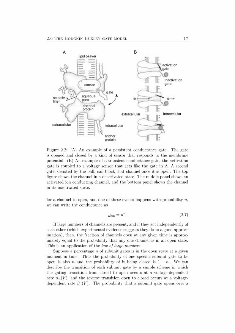
Now, our final point of interest will be how to describe conductancesof specific ions across the membrane. Again, we are mainly interested insodium and potassium and these appear to have two very specific types ofconductance. Potassium has a persistent conductance while sodium has atransient conductance; see figure 2.2.

2.6.1 Persistent conductance

The opening of the persistent conductance gate (we now know) involvesa number of conformational changes (this was unknown at the time ofHodgkin and Huxley). For example, the K+ channel consists of four identi-cal subunits, and it appears that all four must undergo a structural changefor the channel to open. When k identical but independent events are needed


Figure 2.2: (A) An example of a persistent conductance gate. The gateis opened and closed by a kind of sensor that responds to the membranepotential. (B) An example of a transient conductance gate, the activationgate is coupled to a voltage sensor that acts like the gate in A. A secondgate, denoted by the ball, can block that channel once it is open. The topfigure shows the channel in a deactivated state. The middle panel shows anactivated ion conducting channel, and the bottom panel shows the channelin its inactivated state.

for a channel to open, and one of these events happens with probability n,we can write the conductance as

gion = nk. (2.7)

If large numbers of channels are present, and if they act independently ofeach other (which experimental evidence suggests they do to a good approx-imation), then, the fraction of channels open at any given time is approx-imately equal to the probability that any one channel is in an open state.This is an application of the law of large numbers.

Suppose a percentage n of subunit gates is in the open state at a givenmoment in time. Thus the probability of one specific subunit gate to beopen is also n and the probability of it being closed is 1 − n. We candescribe the transition of each subunit gate by a simple scheme in whichthe gating transition from closed to open occurs at a voltage-dependentrate αn(V ), and the reverse transition open to closed occurs at a voltage-dependent rate βn(V ). The probability that a subunit gate opens over a


short interval of time is proportional to the probability of finding the gateclosed, 1−n, multiplied by the opening rate αn(V ). Likewise, the probabilitythat a subunit gate closes during a short time interval is proportional to theprobability of finding the gate open, n, multiplied by the closing rate βn(V ).The rate at which the open probability for a subunit gate changes is givenby the difference of these two terms

dn

dt= αn(ν)(1− n)− βn(ν)n. (2.8)

Now, we can mold this equation into another often used form by dividingby αn + βn, resulting in

τn(ν)dn

dt= n∞ − n, (2.9)

where

τn(V ) =1

αn(V ) + βn(V )(2.10)

and

n∞(V ) =αn(V )

αn(V ) + βn(V ). (2.11)

So what does this equation actually say? It says that for a fixed voltageV , n approaches the value n∞(V ) exponentially with time constant τn(V ).The key elements in the equation for n are the opening and closing ratefunctions αn(V ) and βn(V ). These are obtained by fitting experimentaldata. The data upon which these fits are based are typically obtained usinga technique called voltage clamping; indeed this is what Hodgkin and Huxleyused in their experiments.

2.6.2 Transient conductance

Some channels only open transiently when the membrane potential isdepolarized because they are gated by two processes (subunits) with oppositevoltage dependences; see figure 2.2. One of the gates behaves exactly likethe gate of the persistent conductance. The probability that it is open iswritten as mk where m is an activation variable like n, and k is an integerthat again signifies the number of subunits in the channel (or the numberof events that need to happen for it to open). The probability that the ball(see figure 2.2) does not block the channel is denoted by h and called theinactivation variable.

Now, for the transient conducting channel to be conducting both gatesmust be open, and if the two gates act independently, the probability of thisoccurring is mkh. Thus we can write the transient conductance of a certainion species as

gion = mkh. (2.12)


More generally, if there is not one process blocking the channel butseveral, we could describe this with the following formula for the currentflow due to a certain ion species, sometimes referred to as the Hodgkin-Huxley gating equation

I = gmαhβ(V − Vion). (2.13)

Chapter 3

The Hodgkin-Huxley model

Now that we have found some mathematical descriptions for the variousparts of and processes within neurons we are ready to consider the actualmodel derived by Hodgkin and Huxley. In this thesis we are concernedwith the space-clamped dynamics of the system; that is, we consider thespatially homogeneous dynamics of the membrane. With a real axon thisstate can be obtained experimentally by having a wire down the middle ofthe axon maintained at a fixed potential difference to the outside.

The spatial propagation of action potentials along the nerve axon throughthe concept of travelling waves, is a very interesting and crucial subjectto study, but is not included in this thesis. For the interested reader werefer to Keener & Sneyd - Mathematical Physiology volume I, chapter 6 orto Murray’s Mathematical Biology Volume II, chapter 1.

Here, we will derive the Hodgkin-Huxley model and the reduced analyt-ically tractable FitzHugh-Nagumo model (See FitzHugh 1961, Nagumo etal, 1962) which captures the key phenomena of the HH model.

3.1 The work of Hodgkin and Huxley in per-spective

Now that we have some basic notions under our belt we are in a betterposition to understand the importance of the work of Hodgkin and Huxley.

In 1952, Hodgkin and Huxley wrote five papers (Hodgkin & Huxley a,b, c, d and e) that described their experiments that aimed at determiningthe laws that govern the movement of ions in a nerve cell during an actionpotential.

The first paper examined the function of the neuron membrane un-der normal conditions and explained the basic experimental set-up usedin each of their subsequent studies. The second paper examined the effectsof changes in sodium concentration on the action potential as well as the

20

3.2 Combining the preliminary work 21

Figure 3.1: The inventors of the model, (left) Hodgkin and (right) Huxley.

partitioning of the ionic current into sodium and potassium currents. Thethird paper examined the effects of potential changes on the action poten-tial. The fourth paper outlined how the inactivation process reduces sodiumpermeability.

Hodgkin and Huxley’s accomplishment is really two-fold. Using thealready existing (but at the time, relatively novel) technique of voltage-clamping they were able to gather large amounts of experimental data fromthe giant squid axon. This axon was used because of its size, making itpractical to do experiments on. Secondly they then in their final papersupplied a mathematical model consisting of four non-linear ordinary differ-ential equations, which they showed captured the gathered data quite well,meaning that for certain parameter values action potential like excursionsof the variables can be observed.

The influence of the work of Hodgkin and Huxley can easily be seenwhen opening any textbook on computational neuroscience or mathemat-ical physiology since this subject will always be treated. However, whenopening a biologically oriented textbook this is somewhat harder. Since themathematics of the HH model is considered to complicated, there is oftenlittle mention of Hodgkin and Huxley even though the results of their workare visible in any chapter on action potentials, ion channels and membranes.

The final paper put together all the insights from the earlier papers andrevealed the mathematical model for which they received the 1962 Nobelprize for Physiology and medicine. We will now focus on its derivation.

3.2 Combining the preliminary work

We saw in the previous chapter that the membrane potential for a single-compartment model satisfies

CmdV

dt+ Iion(V, t) = 0,


or, including an applied current

CmdV

dt= −Iion(V, t) + Iapp.

Figure 3.2: The equivalent circuit for the HH model.

This equation can also be arrived at by considering the equivalent circuitof the HH model; see figure 3.2. The cell membrane can be modelled as acapacitor in parallel with an ionic current resulting in the formulas above.

We also saw the concept of linear I-V curves in the previous chapter.There are numerous ions present in the fluids surrounding a cell, howeverthe HH model assumes they can be reduced to two ions and one extravariable in which we lump together all others. This results in

CmdV

dt= −gNa(V − VNa)− gK(V − VK)− gL(V − VL). (3.1)

The previous chapter also covered how to model the conductances interms of activating and inactivating mechanisms. This last step will resultin the actual HH model.

3.2.1 The sodium and potassium conductances

It is important to step back for a moment and revel at the magnitude ofwhat Hodgkin and Huxley did in the following step of the model’s derivation.In the previous chapter we deduced equations for the conductance based onthe assumption of subunits that all have to undergo the same conformationalchange. However, for Hodgkin and Huxley it was the other way around. Thisinterpretation was not available at the time; indeed, they came up with it.To their measurements of sodium and potassium conductances they fittedfunctions m, n and h, and in a stroke of genius gave them the interpretationwe now use.


The specific forms for the conductances they came up with are as follows.For potassium they found

gK = gKn4 (3.2)

where gK is a constant. This formula is to be interpreted as a channelconsisting of four identical subunits. And for sodium they found

gNa = gNam3h (3.3)

where ¯gNa is a constant. This formula is to be interpreted as again con-sisting of four subunits, three of which are activating and one of which isinactivating (think of the ball-like structure in figure 2.2).

3.2.2 Summary of the equations

Combining the results in this chapter we arrive at the full Hodgkin-Huxley model of 4 non-linear ordinary differential equations:

CmdV

dt= −gNam3h(V − VNa)− gKn4(V − VK)− gL(V − VL), (3.4)

where m, h and n are the gating variables that satisfy:

τm(ν)dm

dt= m∞ −m

τh(ν)dh

dt= h∞ − h

τn(ν)dn

dt= n∞ − n

Figure 3.3: (left) The steady-state functions and (right) the time constantsof the HH model. Note: τm is much smaller than the other two. From:Keener & Sneyd, 2nd ed.

Remember that the parameters τm, m∞ etc. are defined in terms of αm,βm etc. and thus have to be estimated from measurements. For the HH

3.3 The dynamics 24

Figure 3.4: (left) The action potential and (right) the gating variables duringthe action potential, both on the same time scale. From: Keener & Sneyd,2nd edition.

model these functions are given in figure 3.3 and figure 3.4. The interestedreader can find the actual expressions and values of the parameters in, forinstance, Keener & Sneyd - Mathematical Physiology Volume I, 2nd ed. (p.206).

3.3 The dynamics

In this section we will explain some features of the dynamics the HHmodel without any proof since these dynamics are not easily investigated.Because of the complexity of the system, various simpler mathematical mod-els, which capture the key features of the full system, have been proposed,the best known and most useful one of which is the FitzHugh-Nagumo model(FitzHugh 1961, Nagumo et al. 1962), which we will derive in the next chap-ter.

If Iapp = 0, the model is linearly stable but excitable. That is, if theperturbation from the steady state is large enough there is a large excursionof the variables in their phase space before returning to the steady state. IfIapp 6= 0 there is a range of values where regular repetitive firing occurs, thatis, the system exhibits limit cycles. These two points remind us of courseof the threshold potential and action potential we discussed in the firstchapter. Both types of phenomena have been observed experimentally andthis indicates that the HH model is very effective at describing what actuallyhappens during the action potential.

The behaviour of periodic orbits as Iapp is increased can be nicely sum-marized in a bifurcation diagram. For each value of Iapp we plot the value ofV at the resting state, and the maximum and minimum values of V over theassociated periodic orbit, see figure 3.5. The point here is just to notice thatthe HH model does indeed produce solutions with the desired behaviour andthat oscillations are possible with increased applied current. Investigation of

3.3 The dynamics 25

Figure 3.5: Bifurcations of the HH model with the applied current Iapp asthe bifurcation parameter. HB denotes a Hopf bifurcation, SNP denotes asaddle-node of periodics bifurcation, osc max and osc min denote, respec-tively, the maximum and minimum of an oscillation, and ss denotes a steadystate. Solid lines denote stable branches, dashed or dotted lines denote un-stable branches From: Keener & Sneyd, 2nd ed.

the bifurcations would require more time than we have here and is thereforeexcluded.

In the following chapter we will focus on explaining the dynamics ofsimplified systems that will also still produce action potential behaviour eventhough the biological context may have been lost. These simplified systemsallow us to more easily investigate the dynamics and we can therefore drawconclusions from their analysis.

Chapter 4

The Fitzhugh-Nagumo model

4.1 History and perspective

In 1961, Fitzhugh sought to reduce the Hodgkin-Huxley model to a two-variable model for which phase plane analysis is applicable. His generalobservation was that the gating variables n and h have slow kinetics relativeto m. Using this he came up with a two-dimensional system that has thesame qualitative features as the HH model. This model is not only namedafter Fitzhugh but also after Nagumo, who in 1962 built the equivalent cir-cuit for the above model (see figure 4.1). In the original papers of FitzHugh,this model was called the Bonhoeffer-van der Pol oscillator because itcontains the Van Der Pol oscillator as a special case.

Figure 4.1: Circuit diagram of the tunnel-diode nerve model of Nagumo etal. (1962)

26

4.2 The fast-slow simplification of the HH model 27

4.2 The fast-slow simplification of the HH model

In the previous chapter we did not include a very detailed descriptionof the dynamics of the HH model. The dynamics would be much easier toinvestigate if the model could somehow be reduced to two dimensions. Thecrucial observation that allows for this follows from the graphs of the gatingvariables of the HH model and their time constants. For ease of referencethese have been included again (see figure 4.2).

Figure 4.2: (left) The gating variables and (right) their associated timeconstants. From: Keener & Sneyd 2nd edition.

To go from four to two dimensions we will have to drop some information,that is unavoidable, but we can try to make reasonable assumptions. Theclearest of which is that the time constant of m, τm, is small or rather fastcompared to the other two constants. Remember that τm signifies the speedwith which m converges on its steady state value m∞. Our first assumptioncould therefore be that that m is instantaneously at this value, i.e. m = m∞.This is called a quasi steady-state approximation.

The second reduction is a bit more obscure. Looking at the graph of thegating variables a symmetry between the graphs of h and n can be seen.Specifically the graph of 1−h and n seem very similar. This can be used toeliminate one of the variables. For instance by setting h = 1−n. Combiningour two assumptions we come upon the simplified Hodgkin-Huxley model(without an applied current) that contains one fast variable V and one slowvariable n

CmdV

dt= −gNam3

∞(V )(1− n)(V − VNa)− gKn4(V − VK)− gL(V − VL)

(4.1)

τn(ν)dn

dt= n∞ − n. (4.2)

4.3 The fast-slow phase plane 28

This is often referred to as the fast-slow model and its phase plane asthe fast-slow phase plane.

4.3 The fast-slow phase plane

Since we have now reduced the model to two variables, we can draw thephase plane for it by considering the nullclines of V and n. Setting dn

dt = 0we find that n = n∞(V ) which is the monotonically increasing function thatwe already know. Similarly setting dV

dt = 0 we find that

V =gNam

3∞(1− n)VNa + gKn

4VK + gLVLgNam3

∞(1− n) + gKn4 + gL,

which has a cubic shape. The nullclines have been plotted in figure 4.3 alongwith an action potential resulting from the dynamics. Notice that for the HHmodel parameters there is one intersection of the nullclines which is thus theonly steady-state of this system. From the signs of dndt and dV

dt we can explainhow this system responds to a perturbation. V is a fast variable and n isa slow variable and they are usually called the excitation and recoveryvariable, respectively. This makes sense since V causes the rise in potential,and n causes the return to the resting state. Because of the relative speeddifferences the trajectories in the phase plane are nearly horizontal excepton the nullcline of V where the flow is vertical. This cubic curve is called theslow manifold. On this curve the trajectories move slowly in the directiondetermined by the sign of dn

dt , but elsewhere the trajectories move quickly

in a horizontal direction, since V is fast. From the sign of dVdt it follows

that trajectories flow away from the middle branch of the slow manifold,meaning in between the local minimum and maximum of the function, andtoward the left or right branches. Thus, the middle branch is called theunstable branch of the slow manifold. This functions as a threshold.When the perturbation from the resting state is so small that V does notcross the unstable manifold, then the trajectories move horizontally towardthe left and return to the resting state, i.e. no action potential is generated.However, if the perturbation is so large that V crosses the unstable manifold,then the trajectory moves to the right until it reaches the right branch ofthe slow manifold. Here dn

dt > 0, and so the solution moves up and along thebranch (since it is stable) until the start of the middle branch is reached (thelocal maximum). There, the flow is nearly horizontal to the left and awayfrom the middle branch, and so the solution moves over to the left branch ofthe slow manifold. Here dn

dt < 0, so the solution moves down and along thisbranch until the resting state is reached again, completing the excursion wehave come to know as the action potential.

If we turn on the applied current in this fast-slow model what happens?As Iapp increases, the V nullcline shifts up, until the two nullclines intersect

4.4 The FitzHugh-Nagumo equations 29

Figure 4.3: The fast-slow phase plane of the Hodgkin-Huxley equations.Both nullclines and an action potential are drawn for Iapp = 0. From:Keener & Sneyd, 2nd ed.

on the middle branch of the cubic. This branch is unstable so the trajectorywill never approach the resting state again, continuously switching betweenthe two stable branches for the same reasons we saw above. This behaviouris called a relaxation limit cycle or relaxation oscillation, see figure 4.4.Biologically, this represents a continuous stream of action potentials.

4.4 The FitzHugh-Nagumo equations

What FitzHugh did was look at a simplified two-dimensional systemthat has the same qualitative characteristics as the fast-slow phase-plane.The system can be represented in several forms but is often written in theabstract form

dv

dt= f(v)− w + Iapp (4.3)

dw

dt= ε(v − γw). (4.4)

Here f(v) is understood to be cubic, just like the V nullcline in the reducedsystem, and Iapp is the same parameter as in the HH model. One form forf(v) that is often used is f(v) = v(1 − v)(1 − α), with α < 1, althoughother choices are available. The nullcline for w is the linear equation w = v

γwhich roughly looks the same as the n nullcline in the reduced HH system.Remember that increasing the Iapp parameter will shift the nullcline of thev upwards, just like we saw in the previous section. Also remember thatthe parameter ε signifies the time-scale difference between the two variables.It is custom to take ε small, thereby making the recovery variable w slowcompared to the excitation variable v, as it should. One of the other ways


Figure 4.4: Fast-slow phase plane of the Hodgkin-Huxley equations, withIapp = 50, showing the nullclines and an oscillation. From: Keener & Sneyd,2nd ed.

the system can thus be represented is by putting ε in the other equation,making dv

dt very large and thus v very fast.

εdv

dt= f(v)− w + Iapp (4.5)

dw

dt= v − γw. (4.6)

The nullclines are assumed to have a single intersection point, which,without loss of generality, is placed to be at the origin and are drawn infigure 4.5.

Now, the analysis of the dynamics of the FitzHugh-Nagumo system isanalogous to the analysis of the reduced HH model, i.e. the two phase planesare basically the same.

When the resting state (the intersection of the nullclines) is on the leftbranch V− and not too far from the minimum W∗, the system is excitable.This is because, as in the reduced model, a sufficiently large perturbationfrom the resting state puts the system on a trajectory that moves away fromthe resting state before eventually returning to rest. Such a trajectory, againjust as in the reduced model, goes to the right branch V+, which it followsas it moves up. When the maximum W ∗ is reached, it moves to the leftbranch V− and then returns to rest, following the branch. See figure 4.6.

As we increased Iapp the reduced HH system produced limit cycles; theFitzHugh-Nagumo system does too. The v nullcline moves up as Iapp in-creases. So, when Iapp takes values in some intermediate range (not too bigbecause then it will lie on the right branch and be stable again), the steadystate lies on the middle branch, V0, and is unstable. Instead of returning to


Figure 4.5: A schematic diagram of the FitzHugh-Nagumo phase plane. V−,V0 and V+ respectively denote the left, middle and right branch we saw inthe reduced model. V− and V+ are stable and V0 is unstable. We denote theminimal value of w for which V(w) exists by W∗, and the maximal value ofw for which V+(w) exists by W ∗. From: Keener & Sneyd, 2nd ed.

rest after one action potential, the trajectory alternates periodically betweenthe left and right branches.

As before with the HH model, the behaviour of periodic orbits as Iapp isincreased can be nicely summarized in a bifurcation diagram. For each valueof Iapp we plot the value of V at the resting state, and the maximum andminimum values of V over the periodic orbit. As Iapp increases, a branch ofperiodic orbits appears in a Hopf bifurcation at Iapp = 0.1 and disappearsagain in another Hopf bifurcation at Iapp = 1.24. Between these two pointsthere is a branch of stable periodic orbits. The bifurcation diagram is drawnin figure 4.8.

This figure shares a lot of its features with the bifurcation diagram ofthe HH model. It helps us understand the dynamics of the HH model just alittle better by making it a lot easier to investigate them. We have lost thebiological interpretation of the variables involved but those are still availablewhen looking at the closely associated HH model. This system of equationthat FitzHugh found has been a cornerstone model for many other subjectsin this field. Its tractability allows easier mathematical analysis and thusmakes it a very popular model.


Figure 4.6: Phase portrait for the FitzHugh-Nagumo system, with α = 0.1,γ = 0.5, ε = 0.01 and no applied current. For these parameter values thesystem has a stable resting state, and is excitable. From: Keener & Sneyd,2nd ed.

Figure 4.7: Phase portrait for the FitzHugh-Nagumo system, with α = 0.1,γ = 0.5, ε = 0.01 and Iapp = 0.5. For these parameter values, the restingstate is unstable and there is a periodic orbit. From: Keener & Sneyd, 2nded.


Figure 4.8: Bifurcation diagram of the FitzHugh-Nagumo equations, withα = 0.1, γ = 0.5, ε = 0.01, with the applied current as the bifurcationparameter. The steady-state solution is labeled ss, while osc max and oscmin denote, respectively, the maximum and minimum of V over an oscilla-tion. HB denotes a Hopf bifurcation point. From: Keener & Sneyd, 2nd ed.From: Keener & Sneyd, 2nd ed.

Chapter 5

Summary

5.1 Review

In this thesis we looked at the problem of finding mathematical modelsfor describing the biological phenomenon of action potential generation.

After a brief introduction to the relevant biology we focused on math-ematical formulations of the basic properties and processes of neurons. Tothis end we started out with the fundamental circuit equation

CmdV

dt= −Iion(V, t) + Iapp.

Then by assuming that the ionic current is composed of only sodium,potassium and a leakage current and that the I-V curves are linear, westumbled upon

CmdV

dt= −gNa(V − VNa)− gK(V − VK)− gL(V − VL) + Iapp.

After that we considered the specific forms of the ionic conductanceswhich we modeled with a simple kinetic scheme and curve fitted the resultingHodgkin-Huxley gating equation to measurements.

All in all we derived the four-dimensional HH model

CmdV

dt= − ¯gNam

3h(V − VNa)− gKn4(V − VK)− gL(V − VL)

τm(ν)dm

dt= m∞ −m

τh(ν)dh

dt= h∞ − h

τn(ν)dn

dt= n∞ − n,

34

5.2 Futher studies 35

where Iapp denotes the externally applied current. This model works quitewell, and the desired behaviour (action potentials) is reproduced by thismodel very nicely.

From this starting point, research went in two directions: one directiontried to make the model even more realistic, taking into account more ionspecies or other phenomena (like synapses etc.). The other direction isa simplification of the model, such that it is possible to see clearly howthe spike is produced. The most important of these simplifications is theFizHugh-Nagumo model that we considered in the next chapter.

We started out by making two assumptions, one about the time constants(m moves fast) and one about the apparent symmetry in h and n. Thisresulted in the fast-slow model

CmdV

dt= − ¯gNam

3∞(V )(1− n)(V − VNa)− gKn4(V − VK)− gL(V − VL)

(5.1)

τn(ν)dn

dt= n∞ − n. (5.2)

After the reduction of the HH model from 4 to 2 variables we reducedeven further and found the FitzHugh-Nagumo equations which are a simplerrepresentation of the dynamics of the fast-slow phase plain

dv

dt= f(v)− w + Iapp

dw

dt= ε(v − γw).

This system in particular appeared to be a very useful model with thesame qualitative features as the HH model and indeed is a standard modelin that virtually every book on the subject of mathematical biology or bio-logical oscillators treats it.

5.2 Futher studies

What we did not get to in this thesis due to a lack of time and the factthat it is an entire topic in itself, is the propagation of these action potentialsthrough travelling waves. For this we refer the reader to the standard textsby Keener & Sneyd and Murray. Or for a very readable introduction totravelling waves in general to the book by Edelstein-Keshet. Rest assuredthough, that it is indeed possible to show that travelling waves exist, at leastfor the FitzHugh-Nagumo system.

There are numerous other subjects that are now ready to be explored.This is one of the reasons why the Hodgkin-Huxley model is so important;it opens doors to all sorts of other interesting problems. Below we name afew fun ones and the relevant literature.

5.2 Futher studies 36

Consider networks of spiking neurons. Such neurons can synchronizeand exhibit collective behaviour that is not intrinsic to any individual neu-ron. For example partial synchrony in cortical networks is believed to gener-ate various brain oscillations, such as the alpha and gamma EEG rhythms.For more, see the book by Izhikevich, Chapter 10.

Other interesting subjects that are perhaps more biological than math-ematical include: synaptic plasticity and learning, for this Gerstner’sbook seems to be a good starting point.

All in all we can conclude that the theory of neuron firing and propaga-tion of nerve action potentials is one of the major successes of mathematicalbiology as a discipline. The contents of this thesis are merely the tip of theiceberg, but a very useful tip nonetheless.

Chapter 6

Sources

• Keener & Sneyd - Mathematical physiology, Volume I: Cellular Phys-iology

• Vander - Human Physiology

• Purves - Neuroscience

• Cronin - Mathematical aspects of Hodgkin-Huxley neural theory

• Abbott & Dayan - Theoretical neuroscience

• Izhikevich - Dynamical systems in neuroscience

• Gerstner - Spiking neuron models

37

modelling neuronal excitation: the hodgkin-huxley...

Documents