modelling and simulation of rainfall-runoff relations for ... · tr civil eng arch citation:...

Citation: Ihimekpen NI, Ilaboya IR, Onyeacholem OF. Modelling and Simulation of Rainfall-Runoff Relations for Sustainable Water Resources Management in Ethiope Watershed using SCS-CN, ARC-GIS, ARC-HYDRO, HEC-GEOHMS and HEC-HMS. Tr Civil Eng & Arch 2(3)- 2018.TCEIA.MS.ID.000136. DOI: 10.32474/TCEIA.2018.02.000136.

206

Modelling and Simulation of Rainfall-Runoff Relations for Sustainable Water Resources

Management in Ethiope Watershed using SCS-CN, ARC-GIS, ARC-HYDRO, HEC-GEOHMS and HEC-HMS

Ihimekpen NI, Ilaboya IR* and Onyeacholem OF

Department of Civil Engineering, University of Benin, Nigeria

Received: May 18, 2018; Published: May 30, 2018

*Corresponding author: Ilaboya IR, Department of Civil Engineering, Faculty of Engineering, University of Benin, P.M.B 1154, Benin City, Edo State, Nigeria, Email:

Research Article

Trends in Civil Engineering and its Architecture UPINE PUBLISHERS

Open AccessL

Abstract

Rainfall-runoff modelling is an integral part of water resources planning and management. Runoff is one of the most important hydrologic variables used in most of the water resources applications and accurate information on the quantity and rate of runoff from land surface into streams and rivers is vital for integrated water resource management since information on runoff is required to deal with many watershed development and management problems.

The aim of the research was to develop a conceptual rainfall-runoff model using River Ethiope as a case study. The input data for the model were annual rainfall data, annual temperature data, daily rainfall data and the digital elevation model (DEM) of the study area. The annual rainfall and temperature data were first analyzed for outliers, homogeneity and normality before used while the HEC-HMS model was calibrated using one month daily rainfall data. The runoff simulation was done by integrating ARC-HYDRO, HEC-GEOHMS, HEC-HMS and ARCGIS.

To develop the runoff model and compute the daily runoff, information on the watershed characteristics were first determined. The initial base flow was assumed to be 0.00, Soil conservation systems (SCS) curve number (CN) for direct runoff value was determined from existing standard tables based on the catchment characteristics, initial abstraction was assumed to be 0.00, Muskingum K (Hr), was calculated using the routing equation, Muskingum X lies between 0.1 to 0.3 for reach while impervious surface (%) was taking as 0.00.

Results obtained shows that the climatic data used for the analysis are homogeneous, devoid of possible outliers, characterized with seasonal variability and do not follow a normal distribution which is expected owing to the stochastic nature of climatic variables. The computed Muskingum k value was 2.2hrs. In addition, results of the runoff simulation shows that the peak discharge from subbasin one was 10.3m3/s, the total precipitation was observed to be 1738.60mm, total precipitation loss was 124.14mm while the total excess precipitation was calculated as 1614.46mm. For subbasin two, the peak discharge was observed to be 9.3m3/s, the total precipitation was observed to be 1738.60mm, total precipitation loss was 113.17mm while the total excess precipitation was calculated as 1625.43mm. For the reach (River), the peak inflow was computed to be 10.3m3/s, the peak outflow was 9.8m3/s while the total inflow was 1609.92m3/s. The time for peak inflow was 17th September, 2016 and the time for peak outflow was observed to be 14th September, 2016.

Keywords: SCS curve number; Base flow, Muskingum K and X; HEC-GEOHMS; HEC-HMS

Abbreviations: SCS: Soil Conservation Systems; DEM: Digital Elevation Model; CN: Curve Number; ANN: Artificial Neural Network; DRO: Direct Runoff

ISSN: 2637-4668

DOI: 10.32474/TCEIA.2018.02.000136

http://dx.doi.org/10.32474/TCEIA.2018.02.000136


Tr Civil Eng & Arch Copyrights@ Ilaboya IR, et al.


227

IntroductionOne of the commonest analyses in hydrological study is surface-

runoff estimation in a watershed based on rainfall distribution. Detailed hydrological studies regarding watersheds especially in real life situation is challenged by lack of sufficient data on one hand and the complexity of hydrological systems on the other hand. These challenges resulted to the inevitable use of rainfall-runoff simulation models. Rainfall-runoff modelling which is an integral part of water resources planning and management is a mathematical model describing the rainfall–runoff relations of a rainfall catchment area, drainage basin or watershed. More precisely, rainfall-runoff model is a relation that produces a surface runoff hydrograph in response to a rainfall event, represented by an input as a hyetograph. In other words, the model calculates the conversion of rainfall into runoff [1]. Since the complete identification, analysis and estimation of all the parameters that affect watershed’s runoff is almost impossible, choosing a suitable model with complete structure, minimum input data requirements and reasonable precision is highly essential to the accurate modelling of rainfall-runoff within a given watershed. One of the hydrologic models that meet these criteria is HEC-HMS which has been widely used in different studies [2-9].

Hydrologic engineering design and management purposes require information about runoff from a hydrologic catchment. Runoff is one of the most important hydrologic variables used in most of the water resources applications. Sound information on the quantity and rate of runoff from land surface into streams and rivers is vital for integrated water resource management since the information is required to deal with many watershed development and management problems. Acquisition and prediction of this information, requires adequate modelling that will bring about the transformation of the rainfall from that catchment to runoff [3]. Models that aids in the transformation of rainfall to runoff can basically be subdivided into three classes and they are: metric (also called data-based, empirical or black box), parametric (also called conceptual, explicit soil moisture accounting or grey box), and mechanistic (also called physically based or white box) model structures.

Numerous studies have been conducted to understand the relation between rainfall and runoff for sustainable water resources management. In a research conducted by Avsek [1] the author concluded that estimation of surface runoff in a watershed based on the rate of received precipitation and quantifying discharge at outlet is important in hydrologic studies. In his study, HEC-HMS hydrological model version 3.4 was used to simulate rainfall-runoff process in Damodar and Kangsabati watershed located in Purulia of West Bengal. Rainfall-runoff simulation was conducted using rainstorm events. Initial results showed that there is clear difference between observed and simulated peak flows. Therefore model calibration with optimization method and sensitivity analysis was done to improve the model performance. It was observed that model validation using optimized lag time parameter showed reasonable

difference in peak flow. It was concluded therefore that HEC-NMS model can be used with reasonable approximation in hydrologic simulation in Damodar and Kangsabati watershed. Finally future prediction of rainfall was made by Thession Polygon method in A2 and B2 scenario of climate change and these inputs were ran using the calibrated HEC-HMS hydrological model to predict the outflows in the years of 2061 to 2090.

In a research conducted by [3] it was concluded that Water resources assessment in poorly gauged and ungauged basins demand supportive rainfall-runoff estimation, while resolving practical water resource management and planning issues. In their study, the research method employed involves rainfall-runoff modelling and simulation with proper efficiency criteria evaluation using the MODMENS modelling platform, a numerical rainfall-runoff semi-distributed GR2M conceptual lumped model. The rainfall-runoff simulation was carried-out in three selected sub-basins of Lower River Niger Basin based on observable discharge dataset. Related error estimation was carried-out to estimate the runoff simulation uncertainty while model optimization approach entails use of Rosen brock-Simplex method and model reliability evaluation entails the use of Nash and Sutcliffe efficiency criteria methods. Result shows a satisfactory model performance at Baro and Makurdi gauging stations (savannah ecological zone) while under-estimation characterizes simulated flow at Onitsha gauging station (Forest ecological region). Seasonally, the model best fit the dry season flow compared to high flow periods (rainy seasons and wetter years).

Oyebode et al. [4] Conducted a research on the use of artificial neural network in rainfall- runoff forecasting. They concluded that in recent time, Artificial Neural Network (ANN) has been found useful in solving engineering problems; its accuracy in forecast of rainfall-runoff for tropical region was investigated in their work. Development of three-layered feed-forward model for rainfall-runoff forecast using gauge height, rainfall and evaporation rates was considered. Levenberg Marquardt’s and Bayesian Regularization were used in training the models with data sets from two selected hydrological gauging stations of Benin-Owena River Basin Development Authority. Multiple Linear Regression model was also developed in order to compare its forecast accuracy with three-layered feed-forward model. The results obtained from the models were evaluated using coefficient of determination and root mean square error as performance statistics. From the results, the model showed higher coefficient of determination and lower root mean square error for the three-layered feed-forward networks. It was concluded that the three-layered feed-forward model improved the forecast accuracy of the runoff of Benin-Owena river basin than multiple linear regression model using the same hydrological condition.

In this study a combination of hydrologic simulation models such as ARCGIS, ARC-HYDRO, HEC-GEOHMS and HEC-HMS were employed in the modelling and simulation of rainfall-runoff


Tr Civil Eng & Arch


Copyrights@ Ilaboya IR, et al.

228

relations for sustainable water resources management in Ethiope watershed.

Research MethodologyDescription of Study Area

River Ethiope was identified to take its source from Umuaja, a town in Ukwani Local Government Area of Delta State. Umutu is the closest town to Umuaja and the two towns’ lies within latitude 5040’ N and longitude 6014’ E. The watershed is located between latitude 5040’N and 5051’N and between longitude 6012’E and 6014’E. It covers a total area of about 250sq.km. It spreads through major towns that include Obiaruku, Abraka, Sapele and empties into the Atlantic Ocean forming a Delta. Southeast of Delta State, within which the watershed is found enjoys a copious rainfall during rainy (monsoon) season. Some part gets flooded during rainy season and then remains dry during summer. The source of River Ethiope is generally in an upland region, where precipitation is heaviest and where there is a slope down from which the run-off can flow, which shows a dendritic drainage pattern. The Geology of the area falls within the deltaic marine sediments of Cretaceous to Quaternary age. There are two principal geological formations in the area namely; Agbada and the Benin Formation. The Benin formation comprises of fluvial gravels and sands. The formation overlies the Agbada Formation. It consists of inter-bedded sand and shale. The two principal geological formations have a relative groundwater regime. They both have reliable groundwater that can sustain regional borehole prediction. The Agbada Formation has little groundwater when compared to the Benin Formation (Figure 1).

Figure 1: Google Earth Imagery Showing River Ethiope.

Data Collection and Pre-Processing

The data needed for this study was collected from the Nigerian Meteorological Center, Warri Delta State Nigeria. The data include annual rainfall and temperature data from 1983 to 2013 and daily precipitation data from 2016 to 2017. Pre-processing of the data was aimed at:

a. Test of Homogeneity

b. Detection of outliers

c. Time series analysis

Detection of Outliers: The labelling rule method was employed to detect the presence of

outliers. The labelling rule is the statistical method of detecting the presence of outliers in the data using the 25th percentile (lower bound) and the 75th percentile (upper bound). The underlying mathematical equation based on the lower and the upper bound is presented as follows:

1 3 1 Q (2.2 ( )Lower Bound Q Q− × − (1)

3 3 1 Bound Q (2.2 ( )Upper Q Q+ × − (2)

At 0.05 degree of freedom, any data lower than Q1 or greater than Q3 was considered an outlier and must be removed before the analysis [2].

Test of Homogeneity: Hydrologic modelling and rainfall frequency analysis requires that the

data be homogeneous and independent. Homogeneity test was carried out to establish the fact that the data used for the analysis are from the same population. Homogeneity test is based on the cumulative deviation from the mean as expressed using the mathematical equation below [5].

k = 1, ---------- n k = 1, ---------- n (3)

Where

= The record for the series X1 X2 ----------- Xn

= The mean

Sks = the residual mass curve

The initial value of Sk = 0 and last value of Sk = n is equal to zero. For a homogeneous record, one may expect that the Sks fluctuate around zero in the residual mass curve since there is no systematic pattern in the deviation Xi’s from the average values. To perform the homogeneity test, a software package (Rainbow) for analyzing hydrological data will be employed [5].

Time Series Analysis: Time series analysis was employed to assess the stochastic nature of

hydrological data. For the time series analysis, hydrological tool (Hydrognomon) was employed to produce the time series plot and estimate the relevant statistics.

Runoff Generation From Precipitation And Temperature Data Using Thornthwaite Monthly Water Balance Soft-ware

Direct runoff data was simulated using the rainfall data and temperature data with the aid of hydrological monthly water balance software (Thornthwaite). The interphase of the Thornthwaite software for simulating direct runoff from rainfall




229

and temperature data is presented figure. Direct runoff (DRO) is runoff, in millimetres, from impervious surfaces or runoff resulting from infiltration-excess overflow. The fraction (drofrac) of Prain that becomes DRO is specified based on design water-balance analyses. Five (5) percent is a typical value to use [9]. The expression for DRO is:

DRO = Prain x drofrac (4)

Direct runoff (DRO) is subtracted from Prain to compute the amount of remaining precipitation

(Premain): Premain = Prain–DRO (5)

Computation Of Outflow Hydrograph Using The Musking-um Equation

In general, the storage in a reservouir is related to the inflow and the outflow by the equation

( (1 )S k Ix x O= + − (6)

Where

S = storage in the reservouir

I = Inflow into the reach

O = Outflow from the reach

K = Constant with dimension of time (t)

X = Number that lies between 0 and 1

If x = 0 then equation (3.6) reduces to:

( )S k O= (7)

Hence if x = 0, it means therefore that there is no inflow then the storage equals the outflow

In the same way if x = 1 then equation (3.6) reduces to

( )S k I= (8)

In which case there is no outflow and the storage (S) equals the inflow

For known values of inflow and outflow, the mean storage will be computed as follows:

( )1 2 1 22 12 2

I I O Ot t S S+ + − = −

(9)

1 2 1 2

2 2I I O Ot t S+ + − = ∆

(9)

Therefore; ( ) ( )( )2 1 2 1 2 1[ 1 ]S S k I I x x O O− = − + − − (10)For a discrete time interval, the following equations were

obtained [6]

( )2 0 2 1 1 2 1 OOutflow C I C I C O= + + (11)

And: 0 1 2 1C C C+ + =

Where:

00.5

0.5kx tC

k kx t− = − − +

(12a)

10.5

0.5kx tC

k kx t− = − + (12b)

2

0.50.5

k kx tCk kx t− − = − +

(12c)

Determination of K And X from the Inflow and Outflow Hydrograph

To determine the value of the Muskingum constant k and x the following procedures was employed:

a) The inflow data into the reach was determined using the Thornthwaite monthly water balance software based on the existing daily precipitation and temperature data

b) With the inflow values now known, then arbitrary values was assumed for the constants C0, C1 and C2 knowing that: C0 + C1 + C2 = 1

c) The outflow from the reach was then computed using the generalized Muskingum equation of the form: ( )2 0 2 1 1 2 1O C I C I C O= + +

d) With the inflow and outflow data now known, the initial inflow hydrograph was then obtained manually in addition with the hydrograph of the routed outflow

e) The difference between the peak value of the inflow hydrograph and the routed outflow hydrograph was taken as the k value

f) For reach modelling the value of x usually lie between 0.1to 0.3 [6].

Estimation of HEC-HMS Model Parameters

The HEC-HMS parameters needed for rainfall runoff modelling include:

a) Initial Base flow

b) Soil conservation systems (SCS) curve number (CN)

c) Initial abstraction

d) Travel time and time of concentration

e) Muskingum K (Hr)

f) Muskingum X (t)

g) Impervious (%)

h) Catchment area (Km2)

HEC-HMS employs the soil conservation systems (SCS) transform method and the Muskingum routing method to perform the rainfall runoff modelling (Hydrologic modelling). The following


Tr Civil Eng & Arch



230

estimation methods and graphical deductions will be employed to get some of the parameters needed to run the model [6].

Results and Discussion

Pre processing of Data

The first stage in the analysis of the data was to look at the descriptive statistics of the annual rainfall records and the annual temperature records. Result of the descriptive statistics is presented in Table 1a & b respectively.

Table 1a: Basic descriptive statistics of annual rainfall data.

Table 1b: Basic descriptive statistics of annual temperature data.

From the result of Table 1a, it was observed that the mean (605.616) is greater than the median (623.8) which is expected for most climatic data. In Table 1b the same trend was observed. The mean value of 32.184 was greater than the median value of 31.800. The observable difference in the computed mean and median of the data is an indication of the variability in the intensity of rainfall and temperature within the period under investigation. In addition, it is often said that climatic data such as rainfall and temperature are not always normally distribution hence it is obvious that we have a high value of skewness and kurtosis as observed in Table 1b.For normality, the skewness and kurtosis should be as close to zero as possible and result of Table 1b gave a skewness value of 2.0175 with a kurtosis of 1.6880 which is far from indicating that the data are not normally distributed. In Table 1a it was observed that the rainfall data are negatively skewed with a skewness value of -0.03814 and a kurtosis value of -0.04052. The fact that the rainfall data are negatively skewed revealed that they are not

normally distributed. A further test of normality was done using the Kolmogorov Smirnov and Shapiro-Wilk test as presented in Table 2a & b.

Table 2a: Test of normality of annual rainfall data.

Table 2b: Test of normality of annual temperature data.

Figure 2a: Normal Q – Q plot of annual rainfall records.

Result of Table 2a & b shows that the significant (p) value of the rainfall data based on the Kolmogorov Smirnov and Shapiro-Wilk test is less than 0.05. For normality p-value must be greater than 0.05. Since our P-value is less than 0.05 we concluded that the annual rainfall data and annual temperature data used in this study are not normally distributed which is expected due to the stochastic nature of climatic variables. The normal probability plot of residual between the observed and expected records shows a complete deviation from the 400 center line as presented in Figure 2a & 2b thus indicating that the annual rainfall data and annual temperature records are not normally distributed. To study the




231

rainfall and temperature pattern within the study area, we obtain the time series plot as presented in Figure 3a & 3b respectively.

Figure 2b: Normal Q – Q plot of annual temperature records.

Figure 3a: Time series plot of annual rainfall records.

Figure 3b: Time series plot of annual temperature records.

The sinusoidal pattern of rainfall and temperature distribution as observed in the plots of Figure 3a & 3b revealed the presence of seasonal variability in the rainfall and temperature data which is a common characteristic of most time series data.

On whether the annual rainfall data and annual temperature data used in this study contain outliers, the labelling rule method for outlier detection was employed. To apply the labelling rule, the 25th and 75th percentile were determined. Table 3 shows the calculated percentiles for the annual rainfall data.

From the result of Table 3 the 25th percentile (Q1) was observed to be 520.70 while the 75th percentile (Q3) was observed to be 671.60 using the weighted average definition.

Table 3: Computed annual rainfall percentiles.

Adopting the labelling rule equation of the form:

1 3 1 Q (2.2 ( )Lower Bound Q Q− × − (6.1)

3 3 1 Bound Q (2.2 ( )Upper Q Q+ × − (6.2)

The lower and upper bound statistics were calculated as follows:

Lower bound = 520.70 – (2.2(671.60 – 520.70)) = 188.72

Upper bound = 671.60 + (2.2(671.60 – 520.70)) = 1003.58

The extreme value statistics of the annual rainfall data which shows the highest and lowest case numbers is presented in Table 4.Table 4: Extreme value statistics of annual rainfall data.

From the result of Table 4 it was observed that the highest rainfall value is 868.4mm which is less than the calculated upper bound of 1003.58mm. The lowest rainfall value was observed to be 354.6 which is greater than the calculated lower bound of 188.72mm. Since no rainfall value was greater than the calculated upper bound or lower than the calculated lower bound, it was concluded that the annual rainfall data used in this study were devoid of possible outliers.

On whether the annual rainfall data used in this study are homogeneous, homogeneity test was conducted. To conduct the homogeneity test, climatic data analysis software (Rainbow) was employed to perform the test.


Tr Civil Eng & Arch



232

The underlying statistics of homogeneity was formulated as follows

H0: Data are statistically homogeneous

H1: Data are not homogeneous

The null and alternate hypothesis were tested at 90%, 95% and 99% confidence interval that is 0.1, 0.05 and 0.01 degree of freedom and results obtained is presented in Figure 4.

Figure 4: Homogeneity test of annual rainfall data.

To ascertain whether or not the annual rainfall data used in this study is homogeneous, homogeneity statistics presented in Table 5 was employed to test the strength of the null hypothesis over the alternate hypothesis.Table 5: Homogeneity statistics of annual rainfall data.

From the results of Table 5 the null hypothesis (H0) was accepted, and it was concluded that the annual rainfall data are statistically homogeneous at 90, 95 and 99% confidence interval.

Generation of Runoff Data Using Thornthwaite Water Balance Tool

Annual runoff data were needed to compute the Muskingum constant (k) which was gotten from the difference between the initial inflow hydrograph and the routed outflow hydrograph. To generate the annual runoff data, annual rainfall and temperature data were analyzed using the Thornthwaite monthly water balance software. Result of the generated runoff is presented in Table 6.

Table 6: Generated runoff using Thornthwaite monthly water balance software.

According to the Thornthwaite monthly water balance software, direct runoff (DRO) is runoff, in millimeters, from impervious surfaces or runoff resulting from infiltration-excess overflow. The total direct runoff generated from the software were then extracted and used as input parameter for the Muskingum routing model for computing the routed outflow.

Computation of Outflow Hydrograph Using Muskingum Routing Equation

Based on the Muskingum routing equation, for a discrete time interval, the following equations were obtained according to Ralf et al., 2006

( )2 0 2 1 1 2 1 OOutflow C I C I C O= + +

And: 0 1 2 1C C C+ + =

Where: 0

0.50.5

kx tCk kx t

− = − − +

10.5

0.5kx tC

k kx t− = − +

20.50.5

k kx tCk kx t− − = − +

For this analysis, the value of C0, C1 and C2 were assumed to be 0.40, 0.25 and 0.35 respectively (Ralf et al., 2006). Result of the routed outflow computation using Muskingum equation is presented in Table 7.

Based on the result of Table 7, the inflow and routed outflow hydrograph was generated as presented in Figure 5.

The peak difference between the inflow hydrograph and the routed outflow hydrograph was used as the Muskingum constant (k). From the result of Figure 5. K value (Muskingum constant) was calculated as approximately 2.2hrs.




233

Table 7: Outflow computation using Muskingum equation.

Figure 5: Generated inflow and routed outflow hydro-graph.

Hydrologic Modelling and Estimation of HEC-HMS Parameters

Figure 6: Digital elevation model (DEM) of study area.

The first step in the hydrologic modelling was the acquisition of the digital elevation model of the River Ethiope and environ. 30m resolution digital elevation model (DEM) was acquired from earth explorer. usgs as presented in Figure 6.

Topographic Analysis: The next step in the hydrologic modelling was to visualize the topographic map of the study area using the digital elevation model. The topo map gave idea about the terrain and possibly the tendency for almost all the rainfall to be converted into direct runoff. The area covered by the DEM was so large that it may be impossible to work on it. As a result, there was need to clip out a section of the DEM for easy analysis using. Figure 7 shows a sectional view of the clipped DEM.

Figure 7: Sectional view of the clipped DEM.

Figure 8: DEM of study area showing places of low and high contour.

To create the topo map, the Hillshade of the area was first created from the clipped DEM. Since topographic maps are naturally generated in feet (ft), then the Hillshade had to be converted to feet (ft). To know the minimum and maximum elevation of the study area, the converted Hillshade was reclassified using the method of Natural break (Jenks).To visualize the general elevation of the study area, the digital elevation model was reclassified into various contour heights. Result of DEM reclassification is presented in Figure 8. From the results of Figure 8 it was observed that areas marked with pink lies within the lowest elevation while areas marked with blue lies within the highest elevation. To visualize some of the towns, cities and places that lie within areas of lowest and highest elevation, the topo map was converted into KML file


Tr Civil Eng & Arch



234

and projected on the Google earth. Result of the projected image is presented in Figure 9.

Figure 9: Projected DEM of study area showing places of low and high contour.

Generation of Input Parameters for HEC-HMS Modelling

A combination of ARCGIS, ARCHYDRO, HEC-GEOHMS and HEC-HMS was employed to simulate the runoff within the study area from daily rainfall data. The HEC-GEOHMS was employed to extract all the basins and sub-basin within the catchment area while the HEC-HMS was employed to simulate the runoff. The following steps were employed during the modelling process.

Fill Sink: This step was used to fill all the depressions located within the study area in other to create a depression less DEM.

Flow Direction: The flow direction process was employed to visualize the direction of flow of all the streams within the study area.

Flow Accumulation: It is the cumulative total of all the flow within the study area.

Stream definition: The stream definition process was employed to visualize all the primary and secondary streams within the study area

Stream Segmentation: Like the stream definition process, stream segmentation helps to segmemtize the stream.

Catchment Grid Delineation: The catchment grid delineation step helps to subdivide the entire catchment area into different basins

Catchment polygon and drainage line processing: The catchment polygon processing, and

the drainage line processing was employed to visualize the drainage lines within each basin. The existing drainage lines as defined by the drainage line processing step are presented in Figure 10. The red lines observed in Figure 10 indicate the drainage lines within each basin.

Ad joint Catchment Processing: Adjoint catchment processing step help to visualize all the

Figure 10: Drainage line processing.

major basins within the catchment that are contributing to flow. Figure 11 shows the output of the adjoint catchment processing step.

Figure 11: Ad joint Catchment processing.

Watershed Delineation: The next step in the hydrologic modelling was to segmemtize the entire basin so as to accurately define the existing sub-basin within each basin (delineation). To achieve this task, project setup analysis was done to delineate the entire watershed and define the existing sub-basin. In the delineation step, one basin was selected from Figure 12 and subjected to series of hydrologic modelling stages to create all the sub-basins. Results of delineation are presented in Figure 12.

Figure 12: Basin delineation.

The various sub-basins within the delineated basin are presented in Figure 13. while the river network within the sub-basin is presented in Figure 14.




235

Figure 13: Visualizing the different sub-basin within a se-lected basin.

Figure 14: River network within the sub-basin.

The direction of flow of the different rivers is presented in Figure 15.while the accumulation of flow is presented in Figure 16. The blue area is the flooded area within the sub-basin.

Figure 15: Flow direction within the sub-basin.

Figure 16: Flow accumulation within the sub-basin.

Basin Characteristics: The first step in modelling the characteristics of the basin was to determine the length and slope of the rivers within the sub-basins. To see the length and slope of the rivers created from the first basin, river attribute Table was generated as presented in Table 8.Table 8: Attribute table of River.

Basin Slope Determination: To determine the basin slope, the watershed slope percent (Wshslope) was first determined using Arc Hydro Tool. The generated watershed is presented in Figure 17 while the basin attribute table showing the calculated basin slope is presented in Table 9.Table 9: Basin attribute table showing the calculated slope, length and area.

Figure 17: Generated watershed within basin A.

Longest Flow Path: This step was used to determine the longest flow path within the basin.


Tr Civil Eng & Arch



236

The longest flow path also help to know the basin time of concentration which is the time taken for the furthest point to start contributing to flow. Figure 18 shows the longest flow path within the basin.

Figure 18: Extracted longest flow path.

Basin Centroid and Centroid Elevation: The basin centroid was employed to determine the center point of all the generated sub-basin. The method used in determining the basin centroid was the center of gravity method. Others methods include; longest floww path and fifty persent area. The generated basin centroid is presented in Figure 19.

Figure 19: Basin Centroid.

Estimation of HEC-HMS Input Parameters: To select the HEC-HMS processes that was employed in estimating the HEC-HMS input parameters, the following standard methods and assumptions were used

a) Soil conservation system (SCS) was employed as the sub-basin loss method

b) Soil conservation system (SCS) was employed as the sub-basin transform method

c) It was assumed that there was no base flow

d) Muskingum routing method was used as the river route method

e) It was also assumed that there was no initial abstraction

Generation of HEC-HMS Schematics: To generate the HEC-HMS schematics for basin

modelling, the entire basin map was first transformed into HMS unit (SI) after which the schematic was generated. The generated HMS schematic is presented in Figure 20.

Figure 20: Generated HMS Schematic.

Simulation of Runoff from Daily Rainfall using HEC-HMS

The first step in the generation of runoff data fron daily rainfall data was to import all the parameters created from the HEC-GEOHMS environment including the HEC-HMS schematic into the HEC-HMS environment as presented in Table 10.Table 10: HEC-HMS environment showing imported model from HEC-GEOHMS.

To generate the daily runoff from the river, two sub-basin and one reach were selected and daily rainfall data for 1st July 2016 to 2nd November 2016 were used as input parameters. The hydrologic parameters of each sunbbasin including the reach are define as follows:

Parameters of Subbasin 1:

a. Area 11.635km2

b. Loss Method SCS curve number method

c. Curve Number 70

d. Transform Method SCS unit hydrograph

e. Base Flow None

f. Imperveous 0.00%




237

Parameters of Subbasin 2:

a. Area 10.580km2

b. Loss Method SCS curve number method

c. Curve Number 72

d. Transform Method SCS unit hydrograph

e. Base Flow None

f. Imperveous 0.00%

Parameters of Reach 1:

a. Routing Method Muskingum

b. Loss/ Gain Method None

c. Muskingum K 2.2

d. Muskingum x 0.3Table 11: Summary result of Subbasin 1 (wet season).

Table 12: Summary result of Subbasin 2 (wet season).

Table 13: Summary result of Subbasin 2 (wet season).

The daily runoff simulation for the two subbasins including the reach was done using the input parameters of section 4.6.1, 4.6.2 and 4.6.3 respectively. The simulation summary results are presented in Tables 11-13 and Figures 21- 23 respectively. The simulated daily runoff is presented in Table 1-12 of attachment.

Figure 21: Simulated flow pattern in Subbasin 1 (wet sea-son).

Figure 22: Simulated flow pattern in Subbasin 2 (wet sea-son).

Figure 23: Simulated flow pattern in Reach 1 (wet season).

From the summary results of runoff simulation, it was observed from (Table 11) that the peak discharge from subbasin one was 10.3m3/s, the total precipitation was observed to be 1738.60mm, total precipitation loss was 124.14mm while the total excess precipitation was calculated as 1614.46mm. For subbasin two, it was observed from (Table 12) that the peak discharge was observed to be 9.3m3/s, the total precipitation was observed to be 1738.60mm, total precipitation loss was 113.17mm while the total excess precipitation was calculated as 1625.43mm. For the


Tr Civil Eng & Arch



238

reach (River), the peak inflow was computed to be 10.3m3/s, the peak outflow was 9.8m3/s while the total inflow was 1609.92m3/s. The time for peak inflow was 17th September, 2016 and the time for peak outflow was observed to be 14th September, 2016.

To verify the robustness of the HEC-HMS tool for rainfall-runoff simulation, daily rainfall data for the months of November, December, 2016 and January, February and March, 2017 representing the dry season were used as input parameters for the simulation and the simulation summary results are presented in Tables 14-16 and Figures 24-25 respectively. To validate the adequacy of the simulation, a comparative analysis was made between the runoff simulation results for the months of July, August September and October representing the wet season and the runoff simulation results for the months of November, December, January, February and March representing the dry season. Tables 17-19 shows the summary results for the wet season and the dry season based on the runoff parameters from subbasin 1, subbasin 2 and the reach.

Figure 24: Simulated flow pattern in Subbasin 1 (dry sea-son).

Figure 25: Simulated flow pattern in Subbasin 2 (dry sea-son).

Figure 26: Simulated flow pattern in Reach 1(Dry Season).

Table 14: Summary result of Subbasin 1 (dry season).

Table 15: Summary result of Subbasin 2 (dry season).

Table 16: Summary results of Reach 1 (Dry Season).

Table 17: Summary Results of Subbasin 1 for Wet and Dry Season.

S/No Runoff Parameters Wet Season Dry Season

1 Peak Discharge (m3/s) 10.3 4.7

2 Total Precipitation (mm) 1738.6 356.9

3 Total Loss (mm) 124.14 103.94

4 Total Excess (mm) 1614.46 252.96

5 Total Direct Runoff (mm) 1609.92 251.47

6 Total Base Flow (mm) 0 0

7 Discharge (m3/s) 1609.92 251.47




239

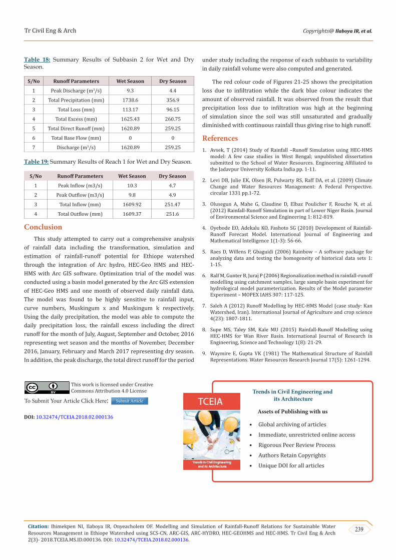
Table 18: Summary Results of Subbasin 2 for Wet and Dry Season.


1 Peak Discharge (m3/s) 9.3 4.4

2 Total Precipitation (mm) 1738.6 356.9

3 Total Loss (mm) 113.17 96.15

4 Total Excess (mm) 1625.43 260.75

5 Total Direct Runoff (mm) 1620.89 259.25

6 Total Base Flow (mm) 0 0

7 Discharge (m3/s) 1620.89 259.25

Table 19: Summary Results of Reach 1 for Wet and Dry Season.


1 Peak Inflow (m3/s) 10.3 4.7

2 Peak Outflow (m3/s) 9.8 4.9

3 Total Inflow (mm) 1609.92 251.47

4 Total Outflow (mm) 1609.37 251.6

ConclusionThis study attempted to carry out a comprehensive analysis

of rainfall data including the transformation, simulation and estimation of rainfall-runoff potential for Ethiope watershed through the integration of Arc hydro, HEC-Geo HMS and HEC-HMS with Arc GIS software. Optimization trial of the model was conducted using a basin model generated by the Arc GIS extension of HEC-Geo HMS and one month of observed daily rainfall data. The model was found to be highly sensitive to rainfall input, curve numbers, Muskingum x and Muskingum k respectively. Using the daily precipitation, the model was able to compute the daily precipitation loss, the rainfall excess including the direct runoff for the month of July, August, September and October, 2016 representing wet season and the months of November, December 2016, January, February and March 2017 representing dry season. In addition, the peak discharge, the total direct runoff for the period

under study including the response of each subbasin to variability in daily rainfall volume were also computed and generated.

The red colour code of Figures 21-25 shows the precipitation loss due to infiltration while the dark blue colour indicates the amount of observed rainfall. It was observed from the result that precipitation loss due to infiltration was high at the beginning of simulation since the soil was still unsaturated and gradually diminished with continuous rainfall thus giving rise to high runoff.

References1. Avsek, T (2014) Study of Rainfall –Runoff Simulation using HEC-HMS

model: A few case studies in West Bengal; unpublished dissertation submitted to the School of Water Resources. Engineering Affiliated to the Jadavpur University Kolkata India pp. 1-11.

2. Levi DB, Julie EK, Olsen JR, Pulwarty RS, Raff DA, et al. (2009) Climate Change and Water Resources Management: A Federal Perspective. circular 1331 pp.1-72.

3. Olusegun A, Mahe G, Claudine D, Elbaz Poulicher F, Rouche N, et al. (2012) Rainfall-Runoff Simulation in part of Lower Niger Basin. Journal of Environmental Science and Engineering 1: 812-819.

4. Oyebode EO, Adekalu KO, Fashoto SG (2010) Development of Rainfall-Runoff Forecast Model. International Journal of Engineering and Mathematical Intelligence 1(1-3): 56-66.

5. Raes D, Willens P, Gbaguidi (2006) Rainbow – A software package for analyzing data and testing the homogeneity of historical data sets 1: 1-15.

6. Ralf M, Gunter B, Juraj P (2006) Regionalization method in rainfall-runoff modelling using catchment samples, large sample basin experiment for hydrological model parameterization. Results of the Model parameter Experiment – MOPEX IAHS 307: 117-125.

7. Saleh A (2012) Runoff Modelling by HEC-HMS Model (case study: Kan Watershed, Iran). International Journal of Agriculture and crop science 4(23): 1807-1811.

8. Supe MS, Taley SM, Kale MU (2015) Rainfall-Runoff Modelling using HEC-HMS for Wan River Basin. International Journal of Research in Engineering, Science and Technology 1(8): 21-29.

9. Waymire E, Gupta VK (1981) The Mathematical Structure of Rainfall Representations. Water Resources Research Journal 17(5): 1261-1294.

Trends in Civil Engineering and its Architecture

Assets of Publishing with us

• Global archiving of articles

• Immediate, unrestricted online access

• Rigorous Peer Review Process

• Authors Retain Copyrights

• Unique DOI for all articles

This work is licensed under CreativeCommons Attribution 4.0 License

To Submit Your Article Click Here: Submit Article

DOI: 10.32474/TCEIA.2018.02.000136


https://digitalcommons.unl.edu/usgspubs/44/



http://www.documentation.ird.fr/hor/fdi:010056972



https://www.researchgate.net/profile/Stephen_Fashoto2/publication/267726466_DEVELOPMENT_OF_RAINFALL-RUNOFF_FORECAST_MODEL/links/56cff5b508ae4d8d649fd08b/DEVELOPMENT-OF-RAINFALL-RUNOFF-FORECAST-MODEL.pdf



https://www.researchgate.net/publication/285816933_RAINBOW-A_software_package_for_analyzing_data_and_testing_the_homogeneity_of_historical_data_sets



http://pakacademicsearch.com/pdf-files/agr/70/1807-1811.pdf



http://stage.ijrests.org/wp-content/uploads/2017/06/3-6.pdf



http://www.lupinepublishers.com/submit-manuscript.php


modelling and simulation of rainfall-runoff relations for ... · tr civil eng arch citation:...

Documents