dynamic modelling of urban rainfall runoff and drainage · dynamic modelling of urban rainfall...
TRANSCRIPT
453810 Analysis and ModellingSummer Term 2012
Dynamic Modelling of Urban Rainfall Runoff and Drainage Coupling DHI MIKE URBAN and MIKE FLOOD
handed in byCadus Sebastian (1122501)Poetsch Marco (0821204)
course instructor AoUniv-Prof Mag Dr Strobl Josef
handover date 08-03-12
i
Introduction gt Urban Rainfall Runoff
Table of Contents
1 Introduction 1
2 Concept 2 21 Urban Rainfall Runoff 2
211 Rainfall 2
212 Rainfall Runoff 4
22 Urban Drainage 6 221 Need for Urban Drainage 6
222 Terminology 7
223 Types of Sewerage Systems 8
23 Introduction to Urban Runoff and Drainage Modelling 9 231 Definition and Purpose of Models 9
232 Model Classifications 10
233 Advantages and Limitations of Models 12
24 Brief Summary 12
3 Method 13 31 Basic Procedure in Urban Flood Modelling 13 32 Model Input Data 15 33 2D Hydrological Modelling in more Detail 17
331 Deduction of Losses 17
332 Important Terms 18
333 Routing Techniques 19
34 1D Hydraulic Modelling in more Detail 22 341 Basic Hydraulic Principles and Terms 22
342 Types of Drainage Flows 25
343 Modelling Sewerage Behaviour 27
35 Types of Model Coupling 28 36 Brief Summary 29
4 Application 30 41 DHI Software 30
411 MIKE URBAN 30
412 MIKE FLOOD 31
42 Model Application 32 421 Model Description 32
422 Study Area 32
423 Model Setup 34
424 Result Interpretation 45
43 Usage of the Model Outcome 48 44 Coupling with Other Software 49 45 Discussion 49
5 Conclusion 52
References ii
List of Figures iv
List of Tables v
List of Formulae v
Table of Content
1
Introduction gt
1 INTRODUCTION Urban flooding and inundation are a serious and inescapable problem for many cities worldwide
However both the spatial scale of these processes and the underlying causes differ significantly Most
cities in the industrialised part of the world are generally confronted with small scale issues often
caused by insufficient capacities of drainage systems during intense rain On the other hand cities in the
developing world experience more severe problems These can usually be traced back to lower sewer
standards and much larger amount of rainfall Such conditions illustrate that accurate simulations of
urban hydrological processes are required in order to predict potential flood threats and to efficiently
improve the designs of sewer infrastructure
It is therefore the purpose of the present paper to dynamically model rainfall runoff in an urban area
This is done by coupling a 2D hydrologic overland model with a 1D hydraulic flow model using the two
software packages of DHI - MIKE URBAN and MIKE FLOOD The overall work is split into three chapters
comprising the concept the method and the actual application The concept block deals with urban
storm events urban drainage infrastructure and gives an introduction into urban runoff and drainage
modelling Thus different rainfall characteristics and their recordings are presented the process of
runoff generation is explained and drainage components as well as different system types are described
Besides the concept of modelling different approaches of model classification and advantages and
limitations of models are highlighted The third chapter on the method focuses on the various flows and
elements of urban runoff modelling required input data 2D- and 1D modelling and the coupling
possibilities between the two models Chapter four is concerned with the application of the software and
the creation of the urban drainage models Here the software packages are specified an overview on
the model the study area and data input is given and the procedure of the model setup is outlined
Furthermore possible usages of the model outcomes are listed potential software couplings are
identified and a critical reflection on the work is given Last a conclusion rounds off the work by
summarising the relevant findings and outcomes
2
Concept gt Urban Rainfall Runoff
2 CONCEPT The following chapter provides an introduction into the basic thematic of this work Consisting of three
parts the chapter deals with rainfall and runoff in urban areas describes different urban drainage
systems as a response to rainfall runoff and introduces into the principles of urban flood models
21 Urban Rainfall Runoff
This abstract brings into focus different characteristics and categories of rainfall and specifies important
terms regarding measurement prediction and rainfall design Further the emergence of runoff in urban
areas is described including the basic processes and flows that occur starting from the rainfall
hyetograph up to the runoff hydrograph
211 Rainfall
Runoff in urban areas is generally caused by rainfall Although there are many different forms of
precipitation such as snow for example rainfall is the most significant contributor to storm water runoff
in most areas (Butler and Davies 201177) Thereby the amount of rainfall changes depending on time
and space When looking at short periods of time and small distances these changes may be small
However they become bigger with increasing time and distance This is due to the fact that space and
time are related to each other (Loucks et al 2005437) Intensive rainfalls tend to originate from small
rain cells (approx one kilometre in diameter) that either last for a short period of time or pass by the
catchment area rapidly Because of their small size the intensity of these types of storms varies
considerably in space On the other hand rainfall events that last for longer typically arise from larger
rainfall cells of large weather systems (Loucks et al 2005437) Thus the spatial difference in intensity is
smaller Depending on the area of the catchment and the number of rainfall measurement stations it is
possible to account for local differences
Moreover rainfall events show an intensity-duration-frequency relationship (IDF) where intensity and
duration are inversely related (Butler and Davies 201182) As Figure 1 illustrates the intensity of an
event decreases with an increasing duration of rainfall Besides it can be seen from the figure that
rainfall intensity and the frequency of an event are backwards related less frequent events tend to be
more intense
Fig 1 Rainfall intensity-duration-frequency diagram (Loucks et al 2005439)
3
Concept gt Urban Rainfall Runoff
At this point it needs to be mentioned that storm events do not just comprise one fixed rainfall depth for
a given duration Rather its intensity alters with time throughout an event (Butler and Davies 201190)
This can be characterised by the peakedness and the skew of the storm in a hyetograph as displayed in
Figure 2 Thus a hyetograph can be defined as a storm profile where rainfall intensity is plotted against
time
Fig 2 Storm peakedness and skew of a storm in a hyetograph (Loucks et al 2005439)
The representation and prediction of rainfall events is a fundamental step in order to take measures
against the effects of rainfall (e g the design and operation of urban drainage) Reference to Butler and
Davies (201177) reveals that this is primarily done by making use of observations - ldquo() the origin of all
knowledge about rainfallrdquo These provide historical records and facilitate the derivation of relationships
between rainfall characteristics A common way of making use of rainfall data is the analysis of long
rainfall records and the definition of their statistical properties Thereby three parameters are generally
utilised to define the statistics of rainfall depth (Locks et al 2005438)
the rainfall intensity (in mm h) or rain depth (in mm) of an event
the duration time period over which the intensity occurs (in min)
the probability of the event to take place in any particular year
For expressing the return period of an event i e the frequency with which an event is likely to occur it
is common practice in the urban context to calculate the inverse of probability (Butler and Davies
201181) To exemplify this an event with a chance of 01 of being matched or even exceeded in any
particular year is expected to return every 101 or 10 years
Locks et al (2005437) have drawn attention to the fact that rainfall events can be split into two
categories namely recorded (real) events and synthetic (not-real) designs The latter can be further
subdivided into stochastically generated rainfall data and design storms Design storms are developed
from actual rainfall data (intensityndashdurationndashfrequency data) and consist of an idealized hyetograph and
a specific return period Their purpose is to reduce the number of runs that are necessary to analyse the
performance of urban drainage systems under specific flow conditions In contrast historical real events
do neither have an idealized hyetograph nor an attached return period (Butler and Davies 201192)
4
Concept gt Urban Rainfall Runoff
Consequently these events are mainly used to verify flow simulation models by providing measured
hyetographs and simultaneous flow observations
Beside these described single events there are also multiple events for both rainfall categories namely
historical time-series and synthetic time-series While historical series represent all measured rainfall at a
certain location and for a specific time period synthetic series can be based on conventional rainfall
parameters (e g storm depth catchment wetness and storm peakedness) (Butler and Davies 201192ff)
Thus the challenge of integrating numerous different events is avoided by taking only few synthetic
storms into account
There is a lot of expert discussion going on concerning the question which of the rainfall events is most
suitable to represent design rainfall (Locks et al 2005437 Butler and Davies 201193) The advantage of
real rainfall time-series is that they take into account many different conditions Thus they are almost
certain to contain the conditions that are critical for the catchment On the other hand a lot of recorded
data and analyses are required and it is difficult to ascertain how suitable the particular portion of
history actually is The argument in favour of using synthetic storms is that they require only few events
to assess the performance of a system and thereforee are easy to utilise However the two methods do
not exclude each other Some syntheses are involved in the use of real rainfall when choosing the
storms to be used in time-series (Locks et al 2005437)
212 Rainfall Runoff
Based on the precipitation data that is available for a catchment area runoff volumes need to be
predicted in order to obtain data for various analyses The relation between precipitation and runoff
depends on a number of rainfall and catchment characteristics (Viessmann and Lewis 1989149) Thus
the lack of detailed basin information such as site-specific land cover imperviousness slope data soil
condition etc may deteriorate the accuracy of the predictions
The actual runoff process includes numerous sub-processes parameters and events as indicated in
Figure 3 Starting with precipitation the rain water falling on the land surface is exposed to various initial
and continuous losses (Zoppou 2001200) Continuous processes are assumed to continue throughout
and beyond the storm event (as long as water is available on the surface) Initial losses encompass
interception wetting losses and depression storage whereas evapo-transpiration and infiltration
represent continuous losses (Butler and Davies 2011108) In the following the whole process is
described more precisely
The first encounters of rainfall water are with intercepting surfaces namely grass plants trees and other
structures that collect and retain the rainwater The magnitude of interception loss depends on the
particular surface type In a second step the remaining water amount may become trapped in numerous
small surface depressions or - contingent on the slope and the type of surface ndash may simply build up over
the ground surface as surface retention (Viessmann and Lewis 198944) Continuing losses such as
infiltration evaporation or leakage may eventually release the retained water again Infiltration in this
context describes the process of water passing through the ground surface into the upper layer of the
soil which is generally unsaturated Penetrating deeper into the soil it may even reach the
groundwater saturated zone Water that has seeped into the soil through the unsaturated zone and
afterwards becomes surface water again is named as inter-flow (Zoppou 2001200) The magnitude of
5
Concept gt Urban Rainfall Runoff
infiltration is reliant on the soil type its structure the compaction moisture content the surface cover
and on the water depth on the soil It can range from 100 for highly permeable surfaces to 0 for
completely impermeable areas Further the infiltration capacity of a particular soil describes the rate at
which the water seeps into it It is usually high at the beginning but tends to diminish exponentially once
the soil becomes saturated (Butler and Davies 2011109) In contrast to infiltration evapo-transpiration
the second process of continuing loss refers to the vaporisation of water directly from the vegetation
and open water bodies Finally the residuary amount of water which is not affected by any of the losses
is called the lsquoexcess rainfallrsquo As described it builds up over the ground surface and once the water film
has accumulated a sufficient depth overland flow sets in (Figure 3) A precondition for this surface flow
to happen is that the rate of surface supply is higher than the rate at which water infiltrates into the
ground (Viessmann and Lewis 198944) Moreover initial-loss depths refer to the minimum quantity of
rainfall that is necessary to cause surface runoff (Loucks et al 2005439) By the time overland flow
reaches defined channels such as roads or natural streams for example the flow changes to a gutter
flow it becomes sewer flow once it enters the underground drainage system
The relative proportions of the different losses and the excess rainfall is not the same for all catchments
Rather they vary both with the characteristics of the surface and with time during the rain event For
instance overland flow usually rises with an increasingly saturated ground (Butler and Davies 20113) In
terms of surface properties urbanisation has a crucial influence on runoff processes Rain falling over a
catchment falls on either an impervious or a pervious surface In the latter case some part of the
rainwater seeps into the ground while the rest becomes surface runoff However in case the water falls
on an impervious area almost the whole rainwater turns into runoff (Zoppou 2001197) Thus due to
the fact that urban areas are typically characterised by extensive impervious surfaces (such as roofs
roads soil compaction and other modifications) they tend to result in increased total surface volume
(Elliott and Trowsdale 2005394) Besides as surface runoff flows faster over solid surfaces than it does
over natural areas the runoff flow occurs and disappears much faster resulting in a higher peak flow
This is also displayed in Figure 4
Fig 3 Schematic description of runoff emergence (Loucks et al 2005440)
6
Concept gt Urban Drainage
Fig 4 Impact of urbanisation on runoff emergence (Butler and Davies 20114)
22 Urban Drainage
In this part measures to deal with urban runoff are presented Thereforee reasons are given that explain
why urban drainage systems are necessary Moreover fundamental terms and components of urban
drainage are defined and a classification schema of drainage systems is outlined
221 Need for Urban Drainage
The effective disposition of rainwater is crucial to protect properties and lives from flooding As
demonstrated this is particularly true for urban areas which are more susceptible to flooding than rural
regions Thus precipitation and the need to collect the resulting runoff are the main purposes of urban
drainage systems (Locks et al 2005437) However there is a second reason also leading back to the
interaction between human and the natural water cycle the need to abstract water and to provide it for
human life (Butler and Davies 20111) Thereforee there are two types of human interaction that
necessitate two types of water to be drained The first one is stormwater i e rainwater that felt on an
impervious built-up area The second type of water is wastewater which is supplied water to support
and maintain a standard of living In both cases the lack of a drainage system would most likely cause
inconvenience damage inundation and health threat For this reason urban drainage deals with both
types of water aiming at a reduction of problems affecting human life and nature
7
Concept gt Urban Drainage
222 Terminology
The work of Viessmann and Lewis (1989307) indicates that drainage systems have been developed from
rather simple ditches to complex systems consisting of curbs gutters surface and underground conduits
Besides Zoppou (2001200) has drawn attention to the fact that urban drainage systems tend to be
more complicated than rural ones as they need to account for numerous additional system features
namely roof top storage open and natural watercourses etc Together with the rising complexity of
these networks comes the need for a more specific knowledge about basic hydrologic and hydraulic
terminology and the processes that take place
In general all storm sewer networks link stormwater inlet points (e g gullies manholes catch pits and
roof downpipes) to either a discharge point or an outfall (Butler and Davies 2011242) This usually
happens through continuous pipes The pipes can be differentiated based on their location in the
network While drains convey flows from individual properties sewers are used to transport water from
groups of properties and larger areas (Butler and Davies 201118) In contrast to sewers the term
lsquoseweragersquo refers to all system infrastructure components including manholes pipes channels flow
controls pumps retarding basins and outlets to name a few
As mentioned before flow in the drainage system comes from the random input of rainfall runoff over
space and time Usually the flows occur periodically and are hydraulically unsteady (Butler and Davies
2011242) According to the magnitude of the storm and the characteristics of the system the network
capacity is loaded to a varying extent in times of low rainfall the runoff amount may be well below the
system capacity whereas during strong rainfall the system capacity may be exceeded This may cause
surcharge pressure flow and even inundation (Chen et al 2005221) Surcharge in this respect means
that a closed pipe or conduit that usually would behave as an open channel runs full and consequently
starts acting as a pipe under pressure However sometimes this is even desirable as it may enhance the
capacity of the drain (Zoppou 2001200)
Figure 5 presents a street that is linked to a drainage pipe via a manhole Here the capacity of the pipe is
suitable to cope with the runoff volume However at this stage it needs to be emphasized that in case of
limited intake capacity through the manhole only a certain part of the runoff will enter the drainage
system despite sufficient pipe capacity (Mark et al 2004286) A situation of insufficient pipe capacity is
shown in Figure 6 In this case the rainwater flows from the drainage system to the street network
causing inundation The duration of the inundation is determined by the intake capacity of the
manholes the pipe capacity as well as by continuous losses namely infiltration and evaporation in the
area (Mark et al 2004286)
Fig 5 Flooding from the street into a part-full pipe of a sewer system (authorsrsquo design based on DHI 200717)
Fig 6 Flooding from a surcharged drainage pipe to the street (authorsrsquo design based on DHI 200718)
8
Concept gt Urban Drainage
The district on the surface that actually adds to the water flow is called the lsquocontributing arearsquo Important
characteristics of the contributing area are its size shape slope land-use roughness soil type wetness
and storage The two properties that impact most on the resulting water volume are catchment area and
land-use (Butler and Davies 2011245)
223 Types of Sewerage Systems
As described urban sewerage systems need to cope with two different kinds of flows namely
stormwater and wastewater As Butler and Davies (201118) perceptively state despite all the progress
that has been achieved the relationship between the carrying of both flows is rather difficult to handle
Thus according to the authors there are very few systems with an ideal solution The most common
types of drainage systems encompass the combined separate and hybrid sewer network as well as the
dual system (Butler and Davies 201118 GEMETEC Limited 20084)
The combined sewer network is the most widespread system in Europe (Butler and Davies 201118)
Thereby both stormwater and wastewater are conveyed together in one singe pipe A schematic graph
illustrating the flow path and interrelationships of this system type is given in Figure 7 As described in
the legend solid errors stand for intentional flows while dotted ones indicate unintentional flows
Moreover thick boxes show flow sources and dashed thick boxes represent sinks Two particular
elements are the combined sewer overflows (CSOs) and the storage which the water runs through
before it is drained to the water treatment plant (WTP) The purpose of these features is the following
While in dry weather the pipes transport wastewater only the amount of flow significantly increases
during rainfall (up to hundred times the usual amount of wastewater) (Butler and Davies 201119) As it
is not cost effective to provide drainage capacity for such conditions the idea is to divert water above a
certain level out of the drainage and into a natural watercourse This is achieved by means of the CSOs
during heavy rainfall an appropriate amount of the storm- and wastewater is conveyed to the WTP
(continuation flow) whereas the excess is transported to a water course (spill flow) (Butler and Davies
201119ff) In case storage is available some water flow may be retained for some time before it is
discharged
The second kind of sewerage system is the separate system As the name implies stormwater and
wastewater are conveyed separately in two pipes usually laid next to each other (Butler and Davies
201120) A schematic graphic is shown in Figure 8 It can be seen that although the wastewater flow
alters significantly during the day the pipes are prepared to transport the maximum water volume all
the way to the WTP Also due to the fact that the stormwater is not mixed with wastewater the whole
amount can be directly drained to a watercourse On the other hand the wastewater sewers transport
the sewage directly to the WTP While the size of the stormwater pipe is approximately the same as the
size of the combined sewer pipe the wastewater pipe is usually smaller (Butler and Davies 201120) One
major problem of this kind of system is that wrong connections and cross-connections at various points
may lead to the undesirable mixing of both flows (Butler and Davies 201126)
9
Concept gt Introduction to Urban Runoff and Drainage Modelling
Fig 7 Combined sewerage system (Butler and Davies 201125)
Fig 8 Separate sewerage system (Butler and Davies 201127)
The third so-called hybrid system is usually composed of a combined sewerage system (often the oldest
parts at the core of the system) and a separate system (generally at the suburban periphery) (Butler and
Davies 201126) In this case the separate wastewater pipes drain into the combined system whereas
the separate storm sewers discharge to receiving waters
Last some cities make use of a dual drainage system consisting of a separate lsquoMajor Drainage Systemrsquo
and a lsquoMinor Drainage Systemrsquo (GEMETEC Limited 20084) The latter is designed to carry flows from
minor storms i e storms with low rainfall intensity and a more frequent return period of two to ten
years On the other hand the major system is suitable to cope with runoff from major rainfall events
The resulting amount of these events would exceed the capacity of the minor system While the minor
system is built up of ditches backyard swales foundation drains and roof leaders major systems usually
comprise ditches open drainage channels and roadways (GEMETEC Limited 20084)
23 Introduction to Urban Runoff and Drainage Modelling
In this section the idea of modelling urban stormwater is introduced First the term lsquomodelrsquo is specified
and their purpose as well as their requirements and field of application in the urban context are
explained Second major categories of models are outlined facilitating a better comparison and
understanding of different models Last important benefits of models are enumerated followed by a
couple of limitations that come with them
231 Definition and Purpose of Models
Viessmann and Lewis (1989493) found that despite the fact that numerous streams have been equipped
with rain gauges to continuously measure flow characteristics there are still many situations where
planners are faced with no or insufficient streamflow information As a consequence of this
mathematical approaches are necessary to create artificial flow sequences that help to investigate the
10
Concept gt Introduction to Urban Runoff and Drainage Modelling
area Simple rules of thumb and rough formulas are usually not appropriate for this purpose (Viessmann
and Lewis 1989307) Thereforee simulation models provide powerful tools to design and operate large-
scale systems of flood control The term lsquosimulationrsquo in this context refers to a mathematical description
of a system response to a given storm event Thus as the two authors have indicated a simulation
model can be specified as ldquo() a set of equations and algorithms hat describe the real system and
imitate the behaviour of the systemrdquo (Viessmann and Lewis 1989498) These mathematical models
consist of algebraic equations with known variables (parameters) and unknown variables (decision
variables) (Loucks et al 200560)
Generally the purpose of sewer system models is to represent a sewerage system and to simulate its
response to altering conditions This helps to answer certain questions such as lsquoWhat ifrsquo scenarios
Butler and Davies (2011470) discovered that there have always been two main application domains for
urban drainage models namely the design of new sewers and the analysis of existing ones When
dealing with the design of a new system the challenge is to determine appropriate physical
characteristics and details to make the model responds satisfactorily in certain situations On the other
hand when analysing existing sewers the physical characteristics of the system have already been
determined (Butler and Davies 2011470) Hence the planner wants to find out about how the system
behaves under certain conditions concerning water depth flow-rate and surface flooding Based on the
result decisions can be made on whether the sewer system needs to be improved and if so how
Given these purposes the model needs to meet a number of particular requirements Zoppou
(2001200f) correctly points out that urban catchments react much faster to storm events than
catchments in rural areas Consequently urban models have to be able to capture and deal with that
rapid behaviour Furthermore a sewer flow model must be able to represent different hydrologic inputs
(rainfall runoff sewer flow) and transform them into relevant information (flow-rate depth pressure)
Thus the main physical processes that occur need to be represented Butler and Davies (2011471)
conclude that the model has to be reasonably comprehensive accurate results can only be derived if no
important process is missed out This also leads to the fact that substantial scientific knowledge about
both hydrologic and hydraulic processes is required Having said that every model is also subject to
simplification as the various interrelationships and feedbacks of reality are too complex to be
represented Based on this Butler and Davies (2011471) correctly argue that - at a general level - there
are three factors that have a considerable impact on both the accuracy and the usefulness of a model
its comprehensiveness
its completeness of scientific knowledge
its appropriateness of simplification
232 Model Classifications
The considerable amount of various simulation models that have been developed and applied provoked
a range of different classification attempts Some of these categorisations are outlined in the following
Turning to Viessmann and Lewis (1989493) one finds that the terms stochastic and deterministic are
commonly used to describe simulation models The differentiation between these two types is rather
straightforward In case one or more of the model variables can be identified as being random and thus
selected from a probability distribution the model is of stochastic nature Thereby model procedures are
based on statistical properties of existing records and estimates always producing a different model
11
Concept gt Introduction to Urban Runoff and Drainage Modelling
response Apart from that a model may be deterministic These models can be considered as stochastic
models where all random variables are replaced by their mean values (Zoppou 2001199) Due to the
lack of random parameters deterministic methods will always deliver the same results for an identical
set of input parameters Viessmann and Lewis (1989497) note that especially deterministic models have
become popular for representing hydrologic behaviour of watersheds
Research by Loucks et al (200569) suggests that simulation methods can be classified into statistical or
process-oriented models or even into a mixture of both Viessmann and Lewis (1989496) use for the
same categorisation the terms lsquodescriptiversquo and lsquoconceptualrsquo Zoppou (2001199) has expressed a similar
view by differentiating between lsquoempiricalrsquo and lsquoconceptualrsquo methods According to the authors
statistical descriptive and empirical models build up on datafield measurements i e observed
phenomena are taken into account Because of this and due to their usage of basic fundamentals
including continuity or momentum conservation assumptions these model types are of particular
interest to hydrologists (Viessmann and Lewis 1989496) On the other hand process-oriented or
conceptual models make use of knowledge on fundamental procedures that are happening Thus these
models rely on theory to interpret certain phenomena rather than representing physical processes
However Loucks et al (200570) observed that a number of models seem to combine elements of both
categories
Simulation models are also classified as physical and mathematical models This in one of the earliest
classification types (Viessmann and Lewis 1989494) Consisting of analogous technologies and basic
principles of similitude physical methods are usually used for small-scale models In opposition to this
mathematical approaches use mathematical statements to represent a system
A fourth classification is achieved considering temporal resolution Thereby temporal resolution alludes
to the smallest computational time step that is used in the model (Elliott and Trowsdale 2005395) The
time step may range from annual average to sub-hourly Hence models can be intended for single storm
events only or for long term continuous processes Based on these differentiations other authors
distinguish between continuous and discrete models (Viessmann and Lewis 1989494) and accordingly
event and continuous process driven (Zoppou 2001199) Thereforee it could be concluded that event
models are short-term models suitable for representing individual storms whereas continuous
simulations model the overall water balance of an area over a long period of time
Moreover catchment models can be classified as either dynamic or static Dynamic models are suitable
to simulate processes including changes over time or even time-varying interactions (Viessmann and
Lewis 1989496) Most hydrologic models belong to this category Besides simulation methods that deal
with time-independent processes are referred to as static
As a sixth and last classification method that is presented in this work models can be separated into
lumped and distributed All three types describe how a particular model deals with spatial variability
(Zoppou 2001199) Models that ignore variations in parameters throughout an entire study area are
called lumped parameter models (Viessmann and Lewis 1989496) In contrast distributed parameter
simulations make allowance for behaviour variations from one location to another As Elliott and
Trowsdale (2005395) have indicated distributed simulations can be further split into quasi-distributed
(model is divided into several elements such as sub-catchments) and fully distributed (often grid-based)
parameter models The majority of urban runoff simulations belong to the distributed category (Zoppou
2001199)
12
Concept gt Brief Summary
233 Advantages and Limitations of Models
It is in the nature of modelling that some system behaviour may be misrepresented to a certain degree
This is mainly due to the mathematical abstraction of real-world phenomena (Viessmann and Lewis
1989497) The extent of deviation i e how much the outputs of the model and the physical system
differ depends on various factors In order to identify differences and to verify the consistency of the
model testing needs to be performed However even verified models tend to have limitations which the
user needs to account for during the analysis Viessmann and Lewis (1989497) claim that especially
when applying models to determine optimal development and operation plans simulation models may
encounter limitations This is because models cannot be used efficiently to develop options for defined
objectives Moreover the authors argue that models tend to be very inflexible regarding changes in the
operating procedure Hence laborious and time demanding programming might be necessary to
investigate different operating techniques Last models carry a certain risk of over-reliance on their
output This is particularly a problem as the results may contain considerable distortions and errors The
fact that models make use of simplifications and ignore random effects makes that clear (Butler and
Davies 2011470) Besides there might be uncertainties associated with the input data or improperly
chosen model parameters which cause biases
On the other hand simulations of hydrologic processes bring numerous important advantages and
possibilities that need to be considered Especially when dealing with complex water flows that include
feedback loops interacting components and relations simulations may be the most suitable and most
feasible tool (Viessmann and Lewis 1989498) Once set up they bring the advantage of time saving and
non-destructive testing Also proposed modifications in the system design and alternatives can easily be
tested compared and evaluated offering fast decision support Butler and Davies (2011470) have
drawn attention to the fact that particularly stochastic models can be of great value in urban drainage
modelling This is due to the fact that randomness in physical phenomena allows for the representation
of uncertainty or the description of environments that are too complex to understand Stochastic
models account for this matter and provide an indication of uncertainty with their output
24 Brief Summary
This part dealt with the general concept of urban rainfall and runoff urban drainage infrastructure and
various modelling categorisations It was found that models and simulations in the field of urban
hydrology imply the use of mathematical methods to achieve two things Either imitate historical rainfall
events or make analyses on possible future responses of the drainage system according to a specific
condition However as was pointed out the results of such models do not necessarily have to be correct
Rather they should be considered useful and taken with a pinch of salt
13
Method gt Basic Procedure in Urban Flood Modelling
3 METHOD This chapter is concerned with methodological approaches of modelling It forms the theoretical base for
the third chapter which puts theory into practice Starting with an introduction to the basic procedure in
urban stormwater modelling both the hydrological and the hydraulic model as well as their relations
and components are elucidated In addition to this basic input data and parameters for both models are
illustrated Subsequent to this the two models are analysed in more detail Thereforee specific terms are
explicated and the crucial procedure is outlined respectively The last section is dedicated to the
combination of both models by means of different coupling techniques
31 Basic Procedure in Urban Flood Modelling
The following abstract describes the relation and derivation of the different elements in an urban runoff
drainage model However it does not deal with the basic development and organisation of a simulation
model which addresses the phases of system identification model conceptualisation and model
implementation (including the model programming) A detailed description of these steps is provided by
the work of Viessmann and Lewis (1989498f)
Most urban stormwater models account for all pertinent phenomena and processes that occur in the
physical runoff drainage system from the input (rainfall) to the output (outflow) Thus on a very general
level these models consist of two basic components (Zoppou 2001199) On the one hand there is
rainfall runoff modelling which is about the generation of surface runoff resulting from precipitation
excess On the other hand transport modelling is involved including the routing of flows through the
rainwater infrastructure Figure 9 illustrates the general procedure and interstage products that are
calculated by both models As an addition to that Figure 10 displays the elements and components of
each model as well as their interactions Besides the hydraulic model is further divided into a pipe flow
and a street flow model
Fig 9 General procedure of a 2D-1D runoff model (authorsrsquo design)
14
Method gt Basic Procedure in Urban Flood Modelling
Fig 10 Interactions between model components of an urban drainage system (Marks et al 2004 287)
The procedure is as follows In a first step a design storm needs to be determined Simple examples of
this would be constant rainfall or being more realistic a rainfall event that has a certain storm profile i
e rain intensity variation over time (see chapter 1) This profile is created together with a particular
return period by making use of IDF relationships Second losses need to be deducted from the design
rainfall in order to calculate the excess rainfall rate As described earlier this is a complex process
because there are many aspects to be taken into account However the opinion of Mark et al
(2004293) is that these losses must only be taken into account if they affect the simulation Hence for
evaporation the authors propose to compare accumulated evaporation to accumulated rainfall in order
to decide whether it should be included Third the remaining runoff (also known as overland flow or the
initial flow of runoff) is routed to the gutter by making use of overland flow equations The physical
processes behind this procedure are very complex including several irregularities on the surface that
impact on the flows and thereforee need to be taken into account In an article by GHKSAR (200050)
flow routing is described as ldquo() a procedure to determine the flow hydrograph at a point in a drainage
system ()rdquo Further the article notes that two methods can be distinguished namely hydrologic and
hydraulic routing While in hydrologic routing the flow is estimated as a function of time based on
upstream inflows and storage attenuation hydraulic routing rates the flow as a function of time and
space throughout the system (GHKSAR 200050) At the end the described processes result in the
transformation of the rainfall hyetograph into a surface runoff hydrograph This hydrograph is the output
of the 2D hydrological model and is usually available for every sub-catchment It serves as input data for
the 1D hydraulic model (Figures 9 and 10)
The 1D transport model is concerned with the gutter and sewer pipe flow routing Thus - going back to
the described process - as a fourth step the gutter flow needs to be routed to the sewer inlet points
15
Method gt Model Input Data
Important at this stage is not so much the volume of water that will enter the pipe drainage system but
rather how long it will take the flow to arrive at the inlet point (Butler and Davies 2011472) In step five
pipe flow routing in the sewer system is operated According to Butler and Davies (2011472) many
software packages represent the sewer system as a collection of lsquolinksrsquo and lsquonodesrsquo In this case links
refer to the sewer pipes holding important hydraulic properties such as the diameter roughness
gradient depth and flow-rate In contrast nodes stand for manholes that may cause head losses or
changes of level
The output of the hydraulic model is an outflow hydrograph It generally consists of simulated changes in
water depth and flow-rate for a certain time period at particular points in the sewer system and at its
outlet points (Butler and Davies 2011473) However in case the capacity of the sewer system is
exceeded by the amount of pipe flow surface flooding becomes an additional component that needs to
be included (Butler and Davies 2011473) This encompasses surcharge modelling in the pipe system and
inundation simulation on the surface To do this the model has to be capable of representing 2D-1D and
1D-2D interactions (compare to Fig 5 and 6) The accuracy of the final model output strongly depends on
the validity of simplifying assumptions that were taken as a basis (Viessmann and Lewis 1989614)
32 Model Input Data
Depending on the complexity and elaborateness of the stormwater model different kind and a varying
amount of input data is required Butler and Davies (2011490) discovered that a conventional system
generally makes use of the data presented in Figure 11 Otherwise in any particular software package
the input data is that which exists for the respective model
Fig 11 Input data and parameters of a conventional stormwater model (authorsrsquo design)
As indicated in the figure a hydrological rainfall runoff model may necessitate a hyetograph defining the
rainfall intensity over time and catchment characteristics Latter includes - amongst other things -
information on the total contributing area the portion of different land-uses soil data and information
on slope ground and pervious impervious areas The hydraulic drainage model in turn utilises the
16
Method gt Model Input Data
generated runoff hydrograph a digital elevation model (DEM) and a derived area-elevation-relation
(AER) diagram as well as a physical definition of the sewerage and the street network An ordinary
sewerage system where manholes are connected through pipes there are generally parameters to be
set for each element As Figure 11 exemplifies for manholes the parameters could comprise ground
level information or a head-loss parameter
In regard to the DEM Butler and Davies (2011481) perceptively state that there is often confusion on
the difference between a DEM and a digital terrain model (DTM) Beyond that Nielsen et al (20082)
refer in their work even to a further term - the digital surface model (DSM) In urban flood modelling a
DTM represents a topographic model of the ground surface only (Butler and Davies 2011481) It forms
the foundation for any flood model In opposition to that a DEM - equal to a DSM - builds up on the
underlying DTM but additionally includes elevation information on buildings trees cars and other
prominent features (Nielsen et al 20082) The purpose of the DEM is to represent land elevation data
This is in need of the estimation of flood volumes on the surface (Mark et al 2004288) Moreover the
resulting inundation map represents water levels that are usually based on the DEM After all a DEM is
also used to develop a AER diagram This diagram is required for surface topography to allow for the
definition of water store capacities during surface flooding (Mark et al 2004291) Hence it becomes
obvious that the accuracy of the final outcomes pretty much depend on the quality of the DEM In regard
to this a study by Mark et al (2004288) shows that for urban flood analysis a horizontal resolution of
the DEM of 1x1 - 5x5 meters is suitable to represent important details including the width of sidewalks
roads and houses Though as found by the authors using a more detailed resolution (e g 1x1m) may
only provide a better visual presentation but does not necessarily bring more accurate results regarding
the flood levels In terms of elevation details (vertical resolution) Mark et al (2004288) claim that the
interval should be in the range of 10-40cm However the work of Gourbesville and Savioli (2002311)
asserts that the DEM must even be able to represent variations of less than 10cm to be realistic
Anyhow the resolution must be sufficient to cover crucial differences particularly the distance between
the road (= crest level of the manhole) and the curb level as shown in Figure 12 If the vertical DEM
resolution is not appropriate to account for these differences the streets must be lsquoburnedrsquo into the
elevation model (Nielsen et al 20082) It is important that the street corresponds to the height of the
curb as streets and major roads act as drains for the surface runoff (see ldquogutter flowrdquo in Figure 3) Thus
in case the water on the street swells above the curb level water will run to adjacent areas and
eventually cause flooding
Fig 12 Distance between curb and crest level (Marks et al 2004292)
17
Method gt 2D Hydrological Modelling in more Detail
33 2D Hydrological Modelling in more Detail
As already mentioned a hydrological model is used to transform a rainfall hyetograph into a surface
runoff hydrograph On a general basis hydrological models can be differentiated into two distinct
classes surface runoff models and continuous hydrological models While latter account for both the
overland and the sub-surface runoff surface runoff models only deal with runoff that appears on the
surface (DHI 201159) Due to the fact that in urban runoff analysis the surface runoff model is the most
commonly used model type it will be subject to investigation in this abstract
The computation of surface runoff resulting from precipitation excess encompass two main parts that
need to be addressed by the surface runoff model the deduction of initial and continuous losses and the
surface flow routing i e the reconversion of the effective rainfall into an overland flow and its passing
to enter the drainage network (Loucks et al 2005439) For this purpose a number of different methods
can be applied most of them make use of general catchment data (e g catchment area size ground
slope) model-specific catchment data and model-specific parameters (DHI 2010c9) Thus in order to be
able to interpret the different outcomes it is important to understand the background and functional
principle of each model as well as the meaning of the main input parameters In the following some
general facts on the deduction of losses are presented and main runoff model parameters and terms will
be explained Subsequent to this most commonly used routing techniques will be outlined
331 Deduction of Losses
The opinion of Loucks et al (2005439) is that the majority of models accounts for initial losses due to
surface wetting and the filling of depression storage Depression storage d (mm) may be described by
the following formula
Formula 1 Representation of depression storage d (in mm)
(authorsrsquo design based on Butler and Davies 2011108)
Thereby k1 represents the (im-)perviousness coefficient of the surface type (ranging from 028 for
pervious to 007 for impervious surfaces) s stands for the ground slope This means that depression
storage is high for rather pervious areas and small ground slope Concerning interception loss Butler and
Davies (2011107) feel that in impervious areas - such as urban environments - the interception loss
tends to be very small in magnitude (lt1 mm) and thus is normally omitted or added to the depression
storage Then again this also depends on the time of the year the particular event and the degree of
imperviousness Initial losses are relatively unimportant during intense summer storms but should not
be neglected in less severe events or in less urbanised areas (Butler and Davies 2011108) In the
modelling process it is common practice to subtract the sum of all initial losses right at the beginning of
the storm to end up with the net rainfall
Turning to continuous losses these processes generally play an important role in urban catchments
especially in areas with large open spaces Nevertheless the effect of evapo-transpiration during short
rainfall events tends to be marginal (Butler and Davies 2011108) Hence in most cases it is omitted or
simply lumped into the initial losses To exemplify this in case of a heavy event (approx 25 mm rainfall
18
Method gt 2D Hydrological Modelling in more Detail
depth) when rain is falling on hot pavement (approx 60degC) a maximum loss of 1 mm may occur (Loucks
et al 2005439) In terms of infiltration the loss rate is usually high at the beginning of an event but
lowers exponentially to a final steady rate once the upper soil is saturated (Butler and Davies 2011109)
This is also expressed in a common formula that is used to represent infiltration Hortonrsquos equation
(Formula 2)
Formula 2 Hortonrsquos equation to account for infiltration (authorsrsquo design based on Butler and Davies 2011109)
In this formula the infiltration rate at time t ft (in mm h) the final infiltration rate fc (in mm h) the
initial rate f0 (in mm h) and the decay constant k2 (in h-1) are included The respective parameters mostly
rely on the soil surface type as well as the initial moisture content of the soil
332 Important Terms
There are several terms and parameters that are frequently used in the context of hydrological
modelling and routing processes Thus to facilitate a better understanding of the techniques described
in the following abstract some definitions are given below
When setting up a surface runoff model an important parameter is the catchment delineation that
needs to be defined This means that the boundaries of the complete catchment (as well as of each sub-
catchment) have to be determined This needs to be done in a way that any rain falling within the
determined area will be directed (by reason of gravity) to a particular point of the local drainage channel
Thereforee both topography and the drainage network need to be understood Butler and Davies
(2011246) state that this is feasible with appropriate accuracy either by means of field work or the
usage of contour maps However as Mark et al (2004290) rightly point out difficulties arise in flat
areas where the boundaries are blurry In this case the authors propose to compare the results of the
model with those in real life and to make according adjustments Beside this manual procedure there is
also a way to automatically delineate the catchment Three common methods are available (Mark et al
2004290)
Distance-based approach Areas are allocated based on their distance to the drainage
network
DEM-based approach Algorithms are used to calculate the most probable flow paths
depending on terrain aspects and slopes in the DEM
DEM plus cover image Equal to the lsquoDEM-basedrsquo approach but with additional information
on land-use from the digital image
A further important parameter - as described earlier - is the type of land-use accompanied by different
degrees of impermeability This factor impacts a lot on the amount of loss respectively runoff Thus
once the total catchment area has been determined the extent and type of the surfaces that drain into
the system need to be enquired A measuring unit for quantifying impervious surfaces is the percentage
imperviousness (PIMP) (Butler and Davies 2011247) It can be derived manually from maps or
automatically from aerial pictures Another way to estimate the PIMP is to make use of the density of
19
Method gt 2D Hydrological Modelling in more Detail
housing in the area Thereforee the following formula may be used where J represents the housing
density (dwellingsha) (Formula 3)
Formula 3 Percentage imperviousness derivation (authorsrsquo design based on Butler and Davies 2011247)
In addition the runoff coefficient C is a parameter that is widely used in surface runoff models The
dimensionless parameter represents the proportion of rainfall that actually adds to the surface runoff
(Butler and Davies 2011247) Its value is dependent on the imperviousness the slope and other
retention properties of the ground Further the work of GHKSAR (200042) shows that C is influenced by
soil characteristics and conditions vegetation cover and the rainfall intensity too Based on the
assumption that impervious surfaces contribute 100 of their rainwater to the runoff and pervious
surfaces add 0 the coefficient can be defined as C = PIMP100 (Butler and Davies 2011247) Although
C has to be somehow related to PIMP it does not necessarily have to be the same as some runoff may
originate from pervious surfaces as well Commonly used runoff coefficient values are displayed in
Table 1 When adopting the given values it is important to investigate and ascertain the respective
conditions on the ground beforehand This is particularly necessary when dealing with unpaved surfaced
as both uncertainties and variability properties tend to be large in this case (GHKSAR 200042)
Surface Characteristics Runoff coefficient C
Asphalt 070 - 095
Concrete 080 - 095
Brick 070 - 085
Grassland (heavy soil)
Flat 013 - 025
Steep 025 - 035
Grassland (sandy soil)
Flat 005 - 015
Steep 015 - 020
Table 1 Runoff coefficient values for particular surface types (authorrsquos design based on GHKSAR 200042)
Last the expression - time of concentration tc - often appears in the hydrological modelling context It
describes the time for surface runoff to flow from the remotest point in the catchment to a point being
under consideration e g the outlet (GHKSAR 200042) Thereforee each location in the catchment has a
different time of concentration Butler and Davies (2011249) further differentiate between two
components of tc the overland flow time also called the time of entry te and the sewer flow time known
as the time of flow tf Te may differ considerably depending on slope surface roughness length of the
flow and rainfall characteristics (e g return period rarer stronger storms result in more water in the
catchment thus faster te)
333 Routing Techniques
Research by Butler and Davies (2011115) suggests that there are currently two types of overland flow
routing techniques that are widely applied namely the unit hydrograph method and the kinematic wave
model The former approach is implemented in numerous different ways and belongs to the group of
20
Method gt 2D Hydrological Modelling in more Detail
linear reservoir models the kinematic wave technique is part of the non-linear reservoir methods Both
techniques and some particular parameters are specified in the following whereat particular emphasis is
put on the unit hydrograph technique
The unit hydrograph refers to the relation between net rainfall and direct runoff (GHKSAR 2000 44) It is
founded on the assumption that effective rain falling over a certain area produces a unique and time-
invariant hydrograph More precisely the method describes the out-flow hydrograph that results from a
unit depth (usually 10 mm) of effective rainwater that falls equally over a catchment area (Butler and
Davies 2011115) This happens at a constant rainfall rate i for a certain duration D For this reason the
system is considered linear and time-invariant The respective response is the D-h hydrograph that is
illustrated in Figure 13 The Y-axis of the D-h unit hydrograph is given as u(D t) - the volume of effective
rain at any time t The duration D is usually 1 hour but can be changed to any time period Using the unit
hydrograph as a base it is possible to develop a hydrograph response to any rainfall event However to
do so the following conditions need to be fulfilled (Butler and Davies 2011115f)
the time base of the unit hydrograph is constant no matter how the rain intensity changes
the ordinates of the runoff hydrograph are proportional to the amount of effective
the response to successive blocks of effective rainfall each starting at particular times may be
obtained by summing the individual runoff hydrographs starting at the corresponding times
Fig 13 The unit hydrograph (Butler and Davies 2011115)
Consequently the direct runoff caused by any net rainfall with different depths for successive
increments of a certain duration may be retrieved by a linear superposition of the responses of the
different net rainfall depths (GHKSAR 200044) This approximate approach is known as convolution and
can be described by the following Formula 4
Formula 4 Equation to process convolution (authorsrsquo design based on Butler and Davies 2011116)
21
Method gt 2D Hydrological Modelling in more Detail
While Q(t) is the runoff hydrograph ordinate at the time t (in msup3 s) the term u(D j) represents the D-h
unit hydrograph ordinate at time j (in msup3 s) Further Iw stands for the rainfall depth in the wth of N
blocks of the duration D (in m) The variable j (in s) can be written as t-(w-1) D Thus the formula allows
calculating the runoff Q (t) at a certain time t of a rainfall event that has n blocks of rainfall with a
duration D
As GHKSAR (200044) has indicated the usage of the unit hydrograph method requires a loss model and
a unit hydrograph In regard to the losses to infiltration the unit hydrograph model assumes that they
can be either described as a fixed initial and constant loss (by the empty-index) as a constant proportional
loss (by the runoff coefficient) or as a fixed initial and continuous loss (by the SCS curve) Turning to the
unit hydrograph this can be derived for a particular catchment through rainfall-runoff monitoring
However if there are no gauges for measurement it may be predicted based on catchments with
similar characteristics Butler and Davies (2011116) propose three methods to do this a synthetic unit
hydrography reservoir models and the time-area method The latter method will be specified in the
following
In case of the time-area method lines are delineated that define equal time of flow travel (isochrones)
from a catchmentrsquos outfall point Thus referring to the abstract that dealt with important terms in the
previous chapter the maximum flow travel time i e the most remote line from the outfall represents
the time of concentration of the catchment By adding up the areas between the different isochrones a
time-area diagram can be created as presented in Figure 14 (lower graphic) This diagram defines the
catchmentrsquos runoff response Describing the whole process from a conceptional point of view the runoff
process in the catchment is split into several cells in the form of concentric circles as shown in the upper
graphic of Figure 14 (DHI 2010c13f) The area of each cell depends on the respective time-area curve
that is used (e g rectangular divergent convergent) it should be chosen to suitably represent the
shape characteristics of the catchment At each time step after the runoff started the accumulated
water amount from every cell moves to the neighbouring cell in downstream direction (DHI 2010c14)
Hence the water volume of each cell is derived as a balance of inflow outflow and the current rainfall
on the cell (multiplied with cell area) The outflow of the last cell in the catchment (outflow) represents
the runoff hydrograph of the catchment
Fig 14 Three examples of a time-area curve (DHI 2010c14)
22
Method gt 1D Hydraulic Modelling in more Detail
Turning to the kinematic wave method a more physically-based approach is presented that aims at
simplifying and solving equations of motion (Butler and Davies 2011129) Using this method the surface
runoff is calculated as an open uniform channel flow being subject to gravitational and friction forces
only The amount of runoff thereby depends on numerous hydrological losses as well as on the size of
the contributing area (DHI 2010c17) Thus the shape of the runoff hydrograph is influenced by surface
parameters of the catchment (including length roughness and slope) which are part of the kinematic
wave computation A widely used formula of the kinematic wave method is the Manning equation in
Formula 5 (Loucks et al 2005432) It can be used to estimate the average velocity V (in m s) and the
amount of flow Q (in msup3s) for a given cross-sectional area A (in msup2) As illustrated the velocity is
influenced by on the hydraulic radius R (in m) and the slope bed S of the channel as well as by a friction
factor n (dimensionless) Typical values for the friction factor according to particular channel material are
given in Table 2
Formula 5 Manningrsquos equation to predict open-channel flow velocity (authorsrsquo design based on Loucks et al 2005432)
Channel material n range
Glass 0009 - 0013
Cement 0010 - 0015
Concrete 0010 - 0020
Brickwork 0011 - 0018
Table 2 Typical values of Manningrsquos n (authorsrsquo design based on Butler and Davies 2011 172)
34 1D Hydraulic Modelling in more Detail
The following abstract covers some basic hydraulic principles that need to be taken into account when
dealing with hydraulic questions in the context of sewer flow modelling Further different categories and
types of drainage flows as well as their specific properties are characterised and common approaches for
the hydraulic modelling process are described
341 Basic Hydraulic Principles and Terms
A fundamental condition in various matters of urban sewerage is the continuity of flow This means that
in a section of conduit with a constant diameter and no cross-sections the mass of liquid that flows into
the conduit at a point one must be equal to the mass that discharges at a point two (Butler and Davies
2011147) Based on the assumption that the density i e mass per unit volume stays the same the
volume entering must be the same as the volume flowing out A second condition that builds up on the
continuity of flow is the continuity of flow-rate the flow-rate (in msup3s or ls) Q1 = Q2 However when
looking at the velocity of the liquid in the pipe there is a difference across the flow cross-section The
maximum velocity can be detected in the centre of a pipe (Butler and Davies 2011148) To make it
23
Method gt 1D Hydraulic Modelling in more Detail
easier to cope with this situation the mean velocity v is defined as the flow-rate per unit area A that is
passed by the flow v = QA
Important parameters that affect the flow in the sewage system are the roughness and the shape of the
pipes Depending on the material condition and age of the pipe there are different values of roughness
ks Common ks values for specific pipe materials are given in Table 3 Thereby the condition lsquonewrsquo refers
to new clean and well-aligned conduits In contrast lsquooldrsquo stands for pipes that are influenced by
biological slime and thus a higher degree of roughness
Pipe material ks range (in mm)
new old
Clay 003 - 015 03 - 30
PVC-U 003 - 006 015 - 150
Concrete 006 - 150 15 - 60
Fibre cement 0015 - 0030 06 - 60
Brickwork - good condition 06 - 60 30 - 15
Brickwork-poor condition - 15 - 30
Table 3 Common values of roughness (authorsrsquo design based on Butler and Davies 2011158)
The shape of a pipe may vary depending on different conditions such as country ground properties and
other things Figure 15 displays some common shapes (including a circular egg-shaped horseshoe and
U-shaped form) as well as their respective geometric and hydraulic properties In most sewerage
systems circular-shaped pipes are used (Butler and Davies 2011167) In terms of geometry this shape
offers the shortest circumference per unit of cross-sectional area For this reason circular shaped pipes
require least wall material to stand both internal and external pressure
Fig 15 Shapes and geometric properties of sewers (Butler and Davies 2011168)
24
Method gt 1D Hydraulic Modelling in more Detail
Depending on the type of drainage conduit as well as on the amount of water that flows within it some
pipes are exposed to water pressure In general pressure may be defined as force per unit area It is
expressed in (kN msup2) or (bar) at which 1 (bar) is equal to 100 (kN msup2) In the hydraulic context
pressure needs to be further differentiated into absolute pressure which refers to pressure relative to
vacuum and gauge pressure i e pressure relative to the pressure in the atmosphere (Butler and Davies
2011147) In hydraulic equations and calculations the latter type is usually used Pressure in a liquid
grows with vertical depth according to the following Formula 6
Formula 6 Components of pressure growth (authorsrsquo design based on Butler and Davies 2011 147)
Thus an increase in pressure ∆p (in N msup2) depends on the product of the liquid density p (in kg msup3) the
gravitational acceleration g (981 m ssup2) and the increase in depth ∆y (in m) In order to express the
energy level of a flowing liquid at any point within the network three components need to be taken into
account (Loucks et al 2005432)
Pressure
Velocity
Potential
These three aspects are commonly represented by a so-called energy head - energy per unit weight - as
indicated in Formula 7 Accordingly the pressure head is pressure per specific weight (N msup2) of the
liquid the velocity head is the quotient of the squared velocity (in m s) and twice the gravitational
acceleration and the potential head is the elevation above some base elevation (in m) The total head H
consists of the sum of all three head components
Formula 7 Representation of pressure head velocity head and potential head (authorsrsquo design based on Butler and Davies 2011150)
The energy level of any flow constantly changes It may increase e g through pumps or decrease e g
due to friction In terms of the energy head this is described through head gains HG and head losses HL
(Loucks et al 2005 432) Figure 16 and 17 point up the energy components for open channel flow and
along a pressure pipe respectively As indicated by the figures the hydraulic grade line HGL represents
the sum of pressure head and elevation head In open-channel flow the HGL coincidences with the water
surface slope as the pressure head at the surface is zero (Figure 16) However for a pressure pipe the
hydraulic head can be expressed as the height to which a water column would build up in a so-called
piezometer - a tube rising from the conduit (Figure 17) (Loucks et al 2005432) Turning to the second
line the energy grade line EGL the sum of the hydraulic grade and the velocity head is described Loucks
et al (2005432) make clear that the EGL represents the height up to which a water column would rise in
a Pitot tube accounting for the velocity of the fluid
25
Method gt 1D Hydraulic Modelling in more Detail
Fig 16 EGL and HGL for an open channel (Loucks et al 2005431)
Fig 17 EGL and HGL for a pipe flowing full (Loucks et al 2005432)
Another aspect that is represented in the last two graphics is the head energy loss It consists of friction
losses and local losses Butler and Davies (2011151) report that friction losses are the result of forces
between the liquid and the wall of the pipe Hence this type of loss occurs along the whole length of the
pipe In contrast to this local losses evolve from local disruptions to the flow e g due to features such as
bends or altering in the cross-section The sum of both components forms the head loss hL
342 Types of Drainage Flows
In the field of hydraulic modelling there are two main types of flow which engineering hydraulics focus
on namely open-channel flow and flow under pressure (Butler and Davies 2011 146) Besides there is a
hybrid type i e a combination of both types which is referred to as part-full pipe flow This is the most
common type of flow in sewer systems (Butler and Davies 2011146) Each type of flow has special
characteristics that need to be accounted for in the modelling process
In order to consider flow to be under pressure the liquid flowing in the pipe has to fill the whole cross-
section of the conduit i e there is no free surface for the whole length of the conduit In such cases the
flow is also described as surcharged flow As Butler and Davies (2011479) point out that it is quite
common for conduits in a drainage system to be surcharged As an example surcharge may occur if
flood volumes exceed the design capacity of a pipe Figure 18 presents a longitudinal vertical part of a
conduit that experiences surcharge and thereforee carries the maximum flow-rate In case of an increase
of water entering the sewer system the capacity of the conduit cannot be raised by an increase in flow
depth As the capacity of a conduit depends on its diameter roughness and the hydraulic gradient the
only way to further increase it is through a rise of the hydraulic gradient (Butler and Davies 2011469)
Thus once the hydraulic gradient rises above ground level manhole surcharge and surface flooding may
occur
26
Method gt 1D Hydraulic Modelling in more Detail
Fig 18 Profile of a pipe flow with surcharge (authorrsquos design based on Butler and Davies 2011169)
Looking at the second type of flow - open-channel flow - liquid carried in a channel flows by gravity
forces with a free surface at atmospheric pressure condition In this case the hydraulic cross-section
alters with the flow (GHKSAR 200045) As already explained in the last chapter the velocity of open-
channel flow can be estimated by means of the Manningrsquos equation (Formula 5) Open-channel flow can
be divided into uniform and non-uniform flow The former type of flow consists of a normal flow depth
meaning that the total energy line the hydraulic grade line and the channel bed are all parallel to each
other (Butler and Davies 2011173) However this is rarely the case as there usually exist alteration in
the pipe slope the pipe diameter or the roughness of the pipe preventing the energy lines from being
parallel Typically in an urban sewerage there is a combination of uniform and non-uniform flow
Part-full pipe flow as a combination of both main flow types is defined as liquid in a conduit that flows
by gravity with a free surface (Butler and Davies 2011146) It is presented in Figure 19 The liquid may
even fill the whole cross-section of the pipe if its flow-rate is equal or higher than the designed pipe
capacity Butler and Davies (2011172) found that for this reason theories on part-full pipe flow are
traditionally more related to those for pipes flowing full though it is rather a special case of open-
channel flow
Fig 19 Profile of a part-full pipe flow (authorrsquos design based on Butler and Davies 2011169)
In addition to the different types of pipe flow the flow in a sewerage can be classified into steady and
constant uniform and accordingly unsteady and non-uniform Steady in this case means constant with
time while uniform refers to constant with distance (GHKSAR 200046) Respectively unsteady means
not constant with time and non-uniform means not constant with distance Thus the following hydraulic
conditions exist
uniform and steady
uniform and unsteady
non-uniform and steady
non-uniform and unsteady
27
Method gt 1D Hydraulic Modelling in more Detail
The flow in the sewers generally tends to be unsteady stormwater alters during a storm event whereas
wastewater changes with the time of day However the opinion of Butler and Davies (2011149) is that it
seems to be unnecessary to account for this altering in a lot of calculations and for reasons of simplicity
conditions can be treated as steady
As another property of the pipe flow the motion can be distinguished into laminar and turbulent The
viscosity of a liquid i e the property that prevents motion is caused by interactions of fluid molecules
that generate friction forces amongst the different layers of fluid flowing at different speed (Butler and
Davies 2011149) If the velocities are high there is an erratic motion of fluid particles leading to
turbulent flow (GHKSAR 200045) On the other hand low velocities result in laminar flow
343 Modelling Sewerage Behaviour
As it was stated above flow in the sewerage is generally unsteady i e it varies with the time of day
Besides the flow tends to be non-uniform due to friction and different head losses along the conduit
For this reason the representation of unsteady non-uniform flow is an important matter when
modelling sewerage behaviour As Butler and Davies (2011474) have indicated there are numerous
methods available to model and analyse unsteady non-uniform flows in a sewerage system Thereby
some methods are founded on approximations whereas others pursue a complete theoretical
investigation of the physics of the flow A very common theoretical method that can be used for
gradually-varied unsteady flow in open channels or part-full pipes is presented by the Saint-Venant
equations In order to make use of the method the following conditions must apply (Butler and Davies
2011475)
there is hydrostatic pressure
the bed slope of the sewer is very small such that flow depth measured vertically tends to be the
same as that normal to the bed
there is a uniform velocity distribution at the cross-section of a channel
the channel is prismatic
the friction losses computed by a steady flow equation is also valid for unsteady flow
lateral flow is marginal
The Saint-Venant equations consist of a dynamic and a continuity equation and can be used to represent
the development of water depth h discharge Q and the mean flow velocity v (Vojinovic and Tutulic
2008184) The dynamic equation is defined in Formula 8
Formula 8 Dynamic equation part of the Saint-Venant equations (authorrsquos design based on Butler and Davies 2011 474)
28
Method gt Types of Model Coupling
Thereby y represents the flow depth (in m) v the velocity (in m s) x the distance (in m) t the time (in s)
So the bed slope and Sf the friction slope respectively without any unit The formula illustrates the three
components that form the equation The first part does not account for changes with distance or time
and thus is valid for steady uniform conditions By including the second term alteration with distance is
factored in Finally the whole equation takes account of variation with time and non-uniform conditions
Formula 9 represents the same equation but transformed according to flow-rate rather than velocity
Besides the Continuity equation is given Q stands for the discharge flow-rate (in msup3 s) the variable A
defines the area of flow cross-section (in msup2) and the term B represents the water surface width (in m)
Formula 9 Momentum and Continuity equation (authorrsquos design based on GHKSAR 2000 51 and Butler and Davies 2011 475)
In short the work of WeiFeng et al (20091615) reveals that the numerical solution above is derived
from a finite differential formulation of the equations according to changing flow-rate and water depths
35 Types of Model Coupling
In regard to the coupling of a hydrological and a hydraulic model there are different ways to define the
relationship between the two models To exemplify this the two models can be coupled in a loose or
tight manner in a sequential or a simultaneous mode and it is feasible to either couple a 1D hydrological
with a 1D hydraulic model (1D-1D) or a 2D hydrological with a 1D hydraulic model (2D-1D) These
possibilities are outlined in the following
Sui and Maggio (199936) have drawn attention to the fact that there is a difference between loose and
tight coupling On a general basis the terms lsquoloosersquo and lsquotightrsquo are a qualitative description of the
coupling Processes in models are said to be tightly coupled if there is a high degree of non-linearity
This means that the interaction between the two models cannot be split into distinct processes which
can be calculated independently from each other and again combined afterwards Thereforee tightly
coupled models may be described as a single unit In contrast to this when defining loosely coupled
models each model makes only little use of the calculations and outcomes of the other one Thus there
is only a small dependency amongst them and the two models may even be derived from two different
software packages (Butler and Davies 2011484) As a consequence the models can be run
independently from each other and outcomes can be combined afterwards in a final solution Taking this
into consideration the decision for a sequential or a simultaneous coupling mode depends to some
degree on the strength of coupling Turning to WeiFeng et al (20091615) one finds that in a sequential
coupling mode the hydrological runoff model can be seen as a pre-processor to create input data for
29
Method gt Brief Summary
the hydraulic drainage model Opposed to that the simultaneous mode coupling implements real-time
interactions between the models As a consequence of this it may be inferred that a tightly coupled
model is necessary in order to run the models in a simultaneous way
As a last method that is described in this work there is 1D-1D and 2D-1D coupling For each approach
both loose and tight coupling is possible Mark et al (2004291) note that in traditional modelling
approaches surcharge water that flew from the sewerage system onto the streets was virtually stored in
a reservoir and returned back to the pipe system once there was sufficient capacity again Butler and
Davies (2011484) observed that the next level of complexity is a loose coupling of a 1D hydrological pipe
model with a 1D flow representation on the urban surface Thus the surface is represented as a series of
interconnected open channels and ponds where the processes are calculated in a similar way as for the
pipe hydraulics Interactions between flows on the ground and those under the ground are disregarded
Applying a more tightly coupled approach the 1D-1D coupling is considered to result in an appropriate
presentation of surface inundation provided that the flow does not spill over the streets (Butler and
Davies 2011484f)
In order to simulate a surcharge-induced flood in an urban area a 1D-2D coupling approach is required
(Hsu et al 200022) This allows for a more accurate prediction of the development of flooded zones and
the estimation of flood depths Especially when making use of tightly coupled 1D-2D models the most
accurate results can currently be achieved (Butler and Davies 2011486) However this is achieved at the
expense of computational power calculation time and data requirements
36 Brief Summary
In can be concluded form this chapter that both the hydrologic overland flow model and the 2D
hydraulic flow model respectively conist of holistic formulae This enables the user of these models to
account for various kind of detaild information concerning the rainfall event the catchment
characteristics and the drainage system At the same time this requires a lot of specific knowledge and
experience in order to find the right constellations of parameters Besides the great number of
adjustment possibilities should not mislead over the fact that models are incapable to include every
detail
30
Application gt DHI Software
4 APPLICATION The following chapter presents the practical part of the work It describes the software which is used as
well as the various parameters which are chosen for the exemplary study area In the end a short
summary and a critical reflection of the software are provided
41 DHI Software
The decision about the software was made in favour of DHI which stands formerly for ldquoDanish Hydraulic
Instituterdquo DHI offers for urban flood simulation two specific software packages that may be used The
first one and likewise the major one is called MIKE URBAN the second one is named MIKE FLOOD
Generally DHI has well-developed software packages with different objectives respectively field such as
environment water and health Furthermore the company offers a range of consulting services DHI
describe itself as an independent and international consulting and research organisation with leading
edge technologies software tools laboratories (chemical and biological) and physical model test
facilities (DHI 2012b)
411 MIKE URBAN
MIKE URBAN is used for modelling the urban water (drainage) network which covers the sewers the
water distribution system and the storm water drainage system which further encompasses the 2D
overland flow Since DHI is cooperating with ESRI the GIS-integration is ensued with components of ESRI
ArcGIS The basic modular structure of MIKE URBAN is shown in Figure 20
Fig 20 Overview of the modular structure (DHI 2012c)
The foundation of MIKE URBAN forms the Model Manager which is included with all license types of
MIKE URBAN The Model Manager is used for the input the manipulation as well as the visualization of
31
Application gt DHI Software
the model data It is also used for illustrating and analysing the results of the simulations As a part of the
Model Manager the SWMM5 engine allows a hydrodynamic computation of the sewer network Built on
top of the Model Manager there are different add-on modules which can be licensed In general it can
be distinguished between the CS (Collection System) -modules for urban dewatering and WD (Water
Distribution) ndashmodules for water supply For an urban flood simulation merely CS-modules are
necessary which are described as follows
Like most CS-modules the ldquoRainfall-Runoffrdquo uses the so called MOUSE engine from DHI The CS-Rainfall-
Runoff includes different hydrological methods such as the time area method the kinematic wave or the
Unit Hydrograph Method (UHM) This rainfall runoff module includes also additional flows as well as the
RDI (rainfall dependent infiltration) These hydrological methods are given within a specified catchment
area whereby in MIKE URBAN a catchment is defined as a geographical feature which represents the
hydrological urban catchments or wastewater drainage areas (AECOM nd1) Finally also the
precipitation plays a role in this module
The ldquoCS-Pipeflowrdquo module includes tools for hydrodynamic computation of the discharge The user can
manage the simulation of specific events as well as hydrodynamic long term series-simulations which
embrace statistical evaluations as well This module includes also the automatic and iterative assessment
of sewer sections (Telegdy 2011)
The ldquoCS-Controlrdquo module serves for the regulation and modification of control structures like pumps and
weirs from a sewer system During a simulation it is possible to intervene this control structures In the
end the ldquo2D Overland Flowrdquo module is a major and important part for an urban flood simulation This
module enables MIKE URBAN to use a MIKE FLOOD simulation in the scope of the software Thus it is
not necessary to use these software packages separately Following the MIKE FLOOD software package
and thereforee this module are described in more detail (Telegdy 2011)
412 MIKE FLOOD
MIKE FLOOD is used for simulating flood plains river flooding storm surge and urban flood studies This
software includes three core elements
MIKE 11 which is a one-dimensional model especially designed for river flooding
MIKE 21 which is used as a two-dimensional overland model
MIKE URBAN model which includes the urban drainage network
With MIKE FLOOD it is possible to couple at least two of these elements respectively models together
The model linkage which has to be used depends on the study area For the urban flood simulation the
coupling of a MIKE 21 model with a MIKE URBAN model might be the best choice The integration of
MIKE FLOOD into MIKE URBAN is only possible for this coupling method and thereforee merely available
for urban flood simulations While this linking method is called ldquoUrban Linkrdquo in MIKE FLOOD it is called
ldquo2D Overland Flowrdquo in MIKE URBAN It is fully integrated into the GIS based GUI or MIKE URBAN For
instance the user can define different inputs like eddy viscosity flooding and drying depth and bed
resistance (For more details see 4233) (DHI 200715ff)
32
Application gt Model Application
42 Model Application
The subsequent part describes the model used as well as the study area Thereforee all parameters
respectively settings and attributes which are necessary for the simulation are described Furthermore
some important (but not used in the model) parameters are described as well For example this paper
describes the functions of weirs and pumps although they are not given in the study area but they could
play an important role in some other urban flood simulations
421 Model Description
A flood event can be caused by different events starting from a heavy rainfall season up to a crevasse In
any case a number of factors like topography exchange with groundwater or land cover influence this
flooding By using software from DHI it is possible to include plenty of these factors to the GIS simulation
Especially an urban flood simulation requires complex modelling for an adequate result Thereforee a
dynamic linkage of different models for the description of all important hydrological processes is
necessary
The foundation of model coupling in urban areas is the 2D digital elevation model For the calculation of
the water movement in the overland detailed knowledge about the terrain character is relevant (Engels
200773) Thus the DEM should have a rather high resolution MIKE URBAN uses the DEM to model
physical processes thereforee slope stream barriers and other terrain characteristics are taken into
account
The coupling of 1-dimensional models for flow modelling and pipe system modelling with the 2-
dimensional model takes place over a spatial allocation of the coupling spots to the raster cells (Engels
76) The shafts (nodes) are linked dynamically to the corresponding raster cells whereby all relevant
hydraulic parameters are committed
Meterological circumstances like rainfall and air temperature can be applied as boundary conditions for
diverse catchments and sub-catchments of the study area Thereby MIKE URBAN can handle continuous
data as well as time-series data Hence it is for example possible to implicit the rainfall intensity for each
minute for a specific catchment By involving these inputs for each catchment a hydrograph is
calculated For the hydraulic module the physical characteristics as well as the connectivity of the 1D
model (pipes manholeshellip) must be described To calculate the 1D gradually varied and unsteady flow
MIKE URBAN is using the Saint-Venant equations (for more information see chapter 343) (AECOM
nd1ff)
The so called MOUSE engine of MIKE URBAN interacts with the 1D and 2D model as well as with the
boundary conditions temporal and spatial dynamically Based on the model categories outlined in
chapter 232 the following model can be described as a dynamic deterministic and distributed model
Since a single storm event is simulated this model can described as an event model
422 Study Area
For the practical part of this assignment it was tried to find a local respectively a regional appealing data
set However since the models (especially the 1D- network model) require a lot of specific information
it was not possible to accomplish this task Furthermore the contact person (Telegdy Thomas) from DHI
also inquired for a suitable data set It was possible to get a dataset of EgebjergDenmark however it
was only suitable for a network simulation and not for a combined 1D2D simulation Anyway the final
33
Application gt Model Application
decision was to use the tutorial data set from DHI which are specially designed for the 2D overland
simulation This data set includes the complete 1D network model with manholes pipes and one outlet
All necessary parameters like the runoff method are provided The DEM consists of a relative high
resolution of 2 meter but objects like streets and buildings are not included Since a DSM offers in many
cases a better result than a DTM a small village with buildings and streets was created in ArcMap The
buildings were added to the DEM with a value of 10 meters while the streets get subtracted from the
DEM with a factor of 20cm Anyway effort was made to use a simulation with both DEMs to get a good
comparison The Figures 22 and 23 visualize the DEMs Generally the study area has a downslope from
South-West to North-East with a coastline on the upper right The altitude difference amounts from 0
(m) at the coast up to 70 (m) in the North
Fig 21 DEM without streets and buildings (authorrsquos design) Fig 22 DEM with streets and buildings (authorrsquos design)
In the 1D model all nodes are defined as manholes except one outlet at the coastline The pipes have a
circular shape and a diameter between 15 (cm) and over 1 (m) Figure 24 shows the manholes (blue) the
outlet (yellow) and the pipes (orange) with the original DEM As boundary condition only the rainfall in
Figure 25 is included which is given as a centenary event Unfortunately since the test data set is not
georeferenced it is not possible to find out about the actual location of the study area
34
Application gt Model Application
Fig 23 1D and 2D Model without streets and buildings (authorrsquos design)
Fig 24 Used rainfall intensity for the model (authorrsquos design)
423 Model Setup
When creating an urban flood simulation it might be the best way to to start with the 1D network
model Therefore it is necessary to create and define the drainage system components like manholes
basins pumps and of course pipes Furthermore it is necessary to define the catchment and each sub-
catchment of the study area If these components are not already given they can be created easily and
in a very similar way as the editor mode in ArcGIS The second part of the model setup forms the 2D
overland model The major part of this model is probably the digital elevation model which should have
of course a very high resolution Furthermore there are still some parameters which have to be defined
The following pages describe the major parameters and settings of both models which have a great
impact to the urban flood simulation
4231 1D Pipe Flow
As mentioned previously the first step is to produce the drainage network which could be done similar
to the Editor Mode in ArcGIS Anyway after all network components are created for each of them
several settings have to be defined
The following stage will describe the major parts of the pipe systems but with a special focus on nodes
and structures as well as pipes and canals since weirs pumps and orifices are not used in our model or
play just a minor part
Nodes and Structures
Beside of some basic information like geometry (diameter) location (ground and bottom level) and of
course the node type itself which could be manhole (Figure 26) basin outlet and so forth there are
35
Application gt Model Application
some more parameters which must be given especially for coupling with the 2D overland According to
this the user has to define the ldquoMax Flowrdquo the ldquoInlet Areardquo and the ldquoQdh factorrdquo as well as the correct
equation to setup the exchange flow between the 1D and 2D model
Fig 25 Manhole in MIKE URBAN (DHI 2010c10)
2D Overland Coupling Settings
With the ldquoMax Flowrdquo the user can define an upper limit to the discharge which is able to flow through
the component The discharge is reduced to this value if the calculated discharge from the flow equation
exceeds this value
The ldquoInlet Areardquo plays merely a role if the orifice equation is defined for describing the flow exchange
between the 1D model elements and the 2D overland model Anyway the greater the cross section the
greater the conveyance capacity of the coupling The inlet area confirms physically to the area of the
manhole cover Acceding to this the parameter is neglected when coupling to a basin (DHI 2011201)
The so called ldquoQdh factorrdquo indicates the water level at which the (calculated) discharge should be
oppressed This ldquosuppression is calculated as the water level difference divided by the Qhd factor to the
power of 4rdquo (DHI 2011201) If instability is caused by a small difference in the water level in the two
models this factor can be used for stabilizing this situation (DHI 2011201)
Furthermore it is also necessary to define the exchange flow of the 2D Overland with the drainage
network Therefore MIKE URBAN offers three different methodsequations
Orifice equation
Weir equation
Exponential function
The ldquoOrifice equationrdquo is more or less the standard used method This equation is defined as follows (DHI
200774)
Formula 10 The orifice calculation (authorsrsquo design based on DHI 2007116)
for |QUM21|lt Qmax where
QUM21 = the flow from the drainage network (sewer) to the overland (MIKE 21 grid point)
HU = the water level of the drainage system
36
Application gt Model Application
HM21 = the ground water level
CD = the discharge coefficient (this should be typically 1)
Am = the cross-sectional area of the manholes
AI = the cross-sectional area of the inlets
The corresponding water level gets overridden by the ground level if the nodes ground level is greater
than the water level of the overland or the water level in the nodes By using the orifice equation it is
necessary to define a coefficient This ldquoorifice coefficientrdquo is a non-dimensional factor which is used to
scale the orifice flow
The ldquoWeir equationrdquo is quite different to the orifice equation This equation is depending on the
ldquoflooding situationrdquo So there are two different calculations for the weir equations according if the
surface is flooded or not In the case that the overland is not flooded the weir equation is calculated as a
free flowing weir as follows (DHI 2007117)
Formula 11 Calculation as a free flowing weir (authorsrsquo design based on DHI 2007117)
for |QUM21|lt Qmax where
Wcrest = the crest width which are used in the equation
CD = the discharge coefficient
If the water level in the nodes is below the ground level of nodes this equation is also used even the
surface is flooded Otherwise the following equation takes place to calculate the weir as a submerged
weir (DHI 2007117)
Formula 12 Calculation as a submerged weir (authorsrsquo design based on DHI 2007117)
The term Hg in these formulae is defined as the ground level at the coupling (DHI 2007117) The Wcrest
ldquoshould be typically be the circumference of the manhole coverrdquo (DHI 2011201)
The third method to define the flow between the overland and the drainage network is the ldquoExponential
functionrdquo This function is using the following formulae (DHI 2007117)
Formula 13 Exponential function (authorsrsquo design based on DHI 2007117)
for |QUM21|lt Qmax where
S = the scaling factor
Exp = the exponent
H is given in meters and Q in msup3s
37
Application gt Model Application
The scaling factor has a linear effect to the discharge Consequently the higher this value the larger the
flow for a certain water level difference between the overland and the sewer model The exponent
factor has a huge influence to the discharge An increase of this value will affect a larger flow for a
specific water level difference between the 1D and 2D model
ldquoThere is an option to suppress oscillations by use of the QdH factorrdquo (DHI 2007117) The value
correlates to the water level difference at which the suppression is referred Especially in cases where
the pressure level in drainage system is close to the water level in the overland model this suppression is
designed for It may be applied individually at each urban coupling By a given value of zero the
suppression will not be applied ldquoThe suppression is factor between zero and one by which the discharge
is multipliedrdquo In the case that the water level difference between the nodes and the overland is greater
than the before described Qdh then the factor will be set to one Otherwise the factor varies as the
water level difference to the power of four (DHI 2007117)
Settings for the study area
For our study area all nodes got for the 2D overland coupling the same values which are
Max flow 010
Inlet area 016
Qdh factor 00
Orifice equation with a coefficient of 098
Q-H relation
Irrespective of the simulation method (1D only or 1D2D) the user has to define the Q-H relation for the
nodes By specifying a Q-H relation for manholes or even basins this Q-H relation will control the
infiltration to these nodes By setting the Q-H relation the user can control the relation between the
infiltration flow and the water level in the manholes However by defining of the Q-H relation for outlets
the user can control the flow behaviour for an outlet The flow which is defined as Q should be given as
a positive value when water flows into the node and negative value when water gets lost from a
drainage network (DHI 201129)
Settings for the study area
Q-H relation was not given for the manholes
Pipes and Canals
Pipes and Canals in MIKE URBAN are defined as one-dimensional water conduits (links) between two
nodes As well as nodes also the pipes need some basic geometric and location information An
important parameter of links is the slope which can be calculated automatically (distance and altitude
difference between the two connected nodes) or typed in by the user The latter can be important when
the link bottom is not equal like the node bottom but rather overhead (Figure 27) However the ending
of a link cannot be below the node bottom
38
Application gt Model Application
Moreover the cross section as well as the material of the links is an important factor for the pipe flow
runoff For the link cross section MIKE URBAN offers four different pipe shapes
Circular
Rectangular
O-Shaped
Egg-Shaped
Fig 26 Left ldquoEgg-Shapedrdquo Pipe Right ldquoO-Shapedrdquo Pipe (DHI 2010b16)
Furthermore it is possible to define own link types with the Cross-section Editor This may be important
when the study area includes special shaped links like natural channels are often like to be Generally it
can be distinguished between opened and closed links The user can therefore decide between a natural
channel and a so called ldquoCRS channelrdquo (cross section shape) For natural channels the shape can be
defined with the ldquoTopography editorrdquo While a CRS channel is defined with just one shape the natural
channel topography is defined as a series of (many) CRSs Figures 28 and 29 visualize a CRS channel once
as an opened link and once as closed link This graphs show the geometry the width the conveyance
the hydraulic radius and the area of the CRS
Fig 27 Open CRS channel (screen-shot taken by the authors) Fig 28 Closed CRS channel (screen-shot taken by the authors)
As already mentioned also the material of the links have an important role for the pipe flow MIKE
URBAN is using the Manningrsquos number to calculate the friction of the links The user can choose one of
the different pre-difined materials (compare to Table 2)
In the end the user can optionally define the maximum discharge for a link This can be done with two
different functions First as a function of the water level in one node or second as a function of the
water level difference between two nodes
39
Application gt Model Application
Settings for the study area
All pipes have a circular shape while the materials are concrete (normal) Therefore the values are
Manning 75
equivalent roughness 00015
H-W coefficient 120
Diameter between 015 and 12 meter
Weirs
DHI referred a weir ldquoas a functional relation which connects two nodes of a MOUSE network (two-
directional flow and submerged flow possible) or is associated with only one node (free flow lsquoout if
system)rdquo (DHI 201136)
While in reality a weir is normally located in a manhole or in a similar construction in MIKE URBAN a
weir is defined as a connection between two nodes This occurs due to numerical solutions for the flow
equations require this circumstance For this model configuration the weirs will be placed between the
nodes as flow connection (DHI 201136)
A weir in MIKE URBAN owns different basic characteristics such as crest level and width orientation and
the type For latter there exists a number of different capabilities like rectangular V-notch trapezoidal
long weirs or CRS weir Depending on which weir type is given some additional parameters have to be
setup
According to the selected weir type there are three different computation methods available the
standard Weir formula the Q-H and the fragmented computation Weirs in MIKE URBAN can be static or
dynamic For the latter one it is possible to control the weirs in ldquoreal timerdquo This can be done with the
RTC (Real Time Control) tool in MIKE URBAN
Finally it is also necessary to enable the ldquoCoupling to 2D overland flowrdquo checkbox Anyway there arenrsquot
any further parameters for the 2-dimensional simulation If the weirs are coupled to the overland model
the discharge of the weir will be added to the overland model as a point inflow which is distributed to
the 2D cells in the coupled area The water level in the 2D model will not influence the weir discharge
further the flow direction within the weir couplings is steadily from the 1D model to the 2D model (DHI
2011202)
Orifices
In the fashion of a weir an orifice in MIKE URBAN is likewise defined as ldquoa functional relationrdquo Moreover
it is as well necessary to define the orifice as connection between two nodes It is possible to define
more than one orifice between the same nodes Figure 30 visualize the computation grid for the orifices
furthermore this is also adaptable for weirs pumps and valves (DHI 201140)
Orifices are specified by the network type which can be storm water waste water or a combination of
both the model type (rectangular circular or CRS) and resultant the diameter as well as the height and
width Additionally it is necessary to define the discharge coefficient and the so called flap gate By
activating flap gates the user can control if a water backflow is possible or not As well as weirs also the
can be controlled with the RTC tool dynamically in real time
40
Application gt Model Application
Fig 29 Difference between real world and model configuration of orifice (DHI 201140)
Pumps
Besides weirs and orifices also pumps are defined as functional relation In the case that the pump is
connected to just one node it is possible to let the water pumped out of the pipe system to the 2D
overland model MIKE URBAN offers different types of pumps namely ldquoConstant flowrdquo ldquoConstant
speedrdquo and ldquoVariable speedrdquo The constant flow pump is probably the ldquoeasiestrdquo type The discharge will
be always the same for these pumps insofar the pump is switched on and acceleration or deceleration
period is not given The so called constant speed pumps have a discharge which will be a ldquofunction of the
actual pressure difference (dH) between the pump wet well and the receiving point in the modelrdquo (DHI
201150)
Figure 31 shows an example of the relationship of discharge and pressure difference The user can define
such a pump curve in MIKE URBAN with the ldquoCurves amp Relationsrdquo tool During the simulation the pump
operates within the range of the dH values in the table So at each calculated time step the actual dH
value gets queried and the corresponding discharge will be determined Much more complex appears
the variable speed pumps For this type of pumps it is necessary to define a number of pump curves
which describes the pump capacity at various percentages of the maximum power input respectively the
maximum rotation speed Figure 32 visualizes an example of these pump curves (DHI 201152)
Fig 30 Relationship of discharge and pressure difference (DHI 201151)
Fig 31 Variable speed pump (DHI 201151)
41
Application gt Model Application
Contrary to the constant pumps it is required to define besides of the maximum capacity (defined by
rotation per minute) also the minimum capacity For coupling the pumps with the 2D model the
checkbox have to be activated Anyway pumps are coupled in the same way to the overland model like
weirs
4232 Catchment
Catchments are essential for every hydrological model Catchments in MIKE URBAN are handled ldquoas
hydrological units where storm runoff and infiltration (RDI) are generated on basis of a single set of
model parameters and input data In fact MIKE URBAN catchments represent the level of spatial
discretization of the hydrological modelrdquo (DHI 201168)
However the geographical boundaries of a catchment do not always suit with the concrete drainage
area Therefore the user can specify a drainage area which would overwrite the actual catchment area
in all hydrological computations (DHI 201168f)
A catchment in MIKE URBAN can be created as polygon in a very similar way as in ArcMap with the Editor
Mode Once a catchment is ldquodrawnrdquo they need to get connected to the network model so the computed
runoff gets into the collection network Thereby it is possible to connect more than one catchment to
one node of the 1D model
4233 2D Overland
DEM and 2D model area
The first step for setting up a 2D overland flow model is choosing the 2D model type itself MIKE URBAN
offers for this model selection three different types
Single Grid
a) ldquoSingle Grid by using a rectangular cell solverrdquo whereby the 2D model area will be covered by
square calculation cell
b) ldquoSingle Grid by using a rectangular multi-cell solverrdquo with the same coverage as type A However
this type is related to a coarser grid where each grid cell is moreover ldquosubdivided into N by N
cells called the fine gridrdquo (DHI 2011192)
Flexible Mesh solver
c) By using the ldquoflexible meshrdquo solver the 2D model will be covered by a grid which exists of a mix
of triangular and quadrangular cells However this opportunity is only available in MIKE FLOOD
in MIKE URBAN this type is currently not supported
2D model parameters
Next up a digital elevation model can be applied whereby the data format has to be an ESRI Grid format
or DHI intern dfs2 format Latter format can be used just in DHI and ESRI products on computers with a
DHI license Furthermore some undisclosed formats depending on installed GIS products could be
applicable
Once the DEM is implemented the ground elevation band can be defined furthermore it is possible to fill
missing values within a specified radius Moreover the cell size as well as the extent of the model area
can be defined
42
Application gt Model Application
Afterwards some model parameters have to get setup such as the ldquoLand valuerdquo the ldquoflooding and
drying depth bed resistance eddy viscosity and rainfall intensity
Land value
The land value can be applied either to define areas where no flooding is expected or to setup a
boundary where flow is not allowed to across (DHI 2011195) Therefore either a user specified value is
added to the highest value of the DEM or a specific elevation hight gets defined
Flooding and drying depth
These two parameters are used to declare which cells are to exclude or reintroduce into the
computation of a simulation DHI declares that the flooding and drying depth is an important mechanism
for 2D overland flow simulations since the runtime of the simulation can be reduced by not spending
computational efforts on simulating cells which are dry Naturally the drying depth must be smaller than
the flooding depth
Bed resistance
Concerning to the Manning number (m13s) the bed resistance coefficient can be specified as constant
value for the whole 2D Model or it can be specified by using an external raster layer
Eddy viscosity
A bit more complex arranged the eddy viscosity By including eddy viscosity the simulation takes eddies
into account The choice of the formula influence how eddies are simulated as a result of flux gradients
(or spatial velocity) The user can choose between the flux based default value (which is defined as E =
002ΔxΔyΔt where Δx and Δy are the cell size of the model and Δt is the time step of the simulation)
or by defining an eddy value and an eddy formulation
Rain DEM
As a last resort the rainfall can be added as an external file to the DEM However the rainfall intensity
can be also included later on as boundary condition
Settings for the study area
Selection of 2D model MIKE 21 Single grid using rectangular cell solver
Land value Highest DEM value + 10 meter
Drying depth 0002
Flooding depth 0003
Bed resistance Constant Manning number agrave 32
Eddy Viscosity Included with default value
43
Application gt Model Application
Fig 32 Settings in MIKE URBAN for the DEM and the 2Dmodel area (screenshot taken by the authors)
Fig 33 2D model parameters in MIKE URBAN (screenshot taken by the authors)
4234 2D Overland Coupling
After the 1D model and the 2D model are finished it is possible to couple them together Therefore
following steps are necessary
selection of the coupling pipe flow components
election of the specific calculation cells
selection of the flow formula for basins and manholes (only necessary if not already done
before)
At first of all it is necessary to couple the pipe flow components with the overland model Usually these
1D model components are manholes however it is also possible to couple with weirs pumps outlets and
basins The coupling of 1D component with specific calculations cells of the 2D model are selected
automatically based on the users defined number of cells or search radius (Figure 35) By defining a
specific number of heightwidth cells a squared area of 2D cells which are nearest to the node getting
selected By defining a radius all cells within the radius (given in meters and starting from each node) will
be included in the coupling area Figure 36 shows coupled nodes with different settings
44
Application gt Model Application
Fig 34 Coupling settings in MIKE URBAN (screen-shot taken by the authors)
Fig 35 Various coupled Nodes to 2D cells (DHI 2011198)
Settings for the study area
Coupling Area Squared area nearest to the node
Number of cells 1
4235 Boundary Conditions
Under ldquoBoundary Conditionsrdquo DHI understand the rainfall intensity and other meteorological
circumstances such as air temperature and evapo-transpiration The rainfall intensity is probably the
major and most important part of setting up boundary conditions In MIKE URBAN the rainfall intensity is
usually given as time-series Therefore the user has to create first of all a ldquoTime-Seriesrdquo file which is
stored as a DHI intern ldquoDFS0rdquo format This can be done with the software tool ldquoTSEditorrdquo which can be
started either within of MIKE URBAN or external In any case it is possible to define the rainfall intensity
very much in detail (Figure 37) The rainfall as well as other boundary conditions can be applied to the
whole study area or just for specific catchments For the first case coordinates can optionally be
specified
Fig 36 TSEditor for the rainfall intensity (screen-shot taken by the authors)
45
Application gt Model Application
4236 Set up and Running the Simulation
Setting up the simulation takes only few steps into account Howsoever it is necessary to define the
simulation type as ldquoNetwork + 2D overlandrdquo Furthermore the simulation period some outputs (like the
flood map) and the computation time steps have to get defined
The outputs usually are stored as DHI intern formats like DFS2 for the flood maps DFS0 for time-series
and CRF for the network model Latter includes the discharge of the 1D model and is necessary for
hydrodynamic calculations
A major specification of the simulation is the hydrological model As already mention in chapter 33
there exists different concepts for simulating a surface runfoff DHI offers thereforee four different
models (DHI 2010c9)
Model A Timearea (with or without RDI)
Model B Non-linear Reservoir (kinematic wave) (with or without RDI)
Model C Linear Reservoir
o Model C1 Dutch runoff model
o Model C2 French runoff model
UHM Unit Hydrograph Model (with or without RDI)
Each of these models uses different runoff computations concepts and model parameters as well as a
different set of input data It is not possible to combine the computations within one simulation for
various model areas For the Models A B and C it is possible to include continuous runoff components
like the rainfall-induced infiltration Howsoever some implementations as well as the rainfall-induced
infiltration require additional DHI licenses
The user has to decide which of the models fits best to his application respectively to the catchments
Thereforee it is indispensable that the user understand the background of each model The appreciation
of the used runoff computations which is applied in the model ldquoas well as the meaning and the
interrelation of the various data and model parametersrdquo is necessary (DHI 2010c9)
For this study the Unit Hydrograph Model was used for simulating the rainfall runoff
Settings for the study area
Runoff Model Type UHM
Time step 05
424 Result Interpretation
Following an overview of the simulation results for the 1D network model as well as for the 2D overland
model are given The interpretation of the 1D model is necessary to understand in a better way the
overland flooding since the pipe network interacts with the overland via manholes and outlets Figure
38 visualises a pipe section of the study area at a specific time (1159 am) It is readily identifiable that
the pipes in the lower section are overloaded and how the manholes get overfilled and discharge the
water to the overland
46
Application gt Model Application
Fig 37 Specific pipe section of the study area at 1159 AM (authorrsquos design)
By a reflection of the overland at the same time it is discernible how the overland is flooded equally in
the lower section
With a look to rainfall intensity (see figure 37) which has the peak around 12 am it is identifiable that it
took quite a long time until the overland situation gets more or less relaxed While after the heavy
rainfall the flooding goes relative quickly back in the higher parts of the study area in the lower parts the
flooding is still increasing The maximum flood extent is around 1 pm
The comparison of the simulations once with the DTM and once with the DSM confirmed the
importance of objects in a digital elevation model Especially by interpreting the simulation as video it is
clearly recognizable how the streets officiate as channels (see clip 1 and 2) Furthermore areas with
buildings cannot be flooded anymore consequently the water has to find another way Map 1 visualizes
the maximum flood extent during the calculated time period
Rendering Time
162 minutes
Computer specification
Win 7 Home Edition
8 processors
12GB RAM
Intel i72600 - 34 Ghz
1GB external graphic card
47
Application gt Model Application
Fig 38 Study Area with the flood extent at 1159 AM (authorrsquos design)
48
Application gt Usage of the Model Outcome
Clip 1 Flooding scene with buildings and streets (authorrsquos design) Clip 2 Flooding scene without buildings and streets (authorrsquos design)
43 Usage of the Model Outcome
There are several possibilities how the outputs of the simulation can be used One common way is the
creation of a flood risk assessment map For this purpose the maximum flood extent can be exported
directly as a map in diverse formats Beside of others it is possible to export the map respectively the
files as a GeoTIFF whereby further adaption with other software products is possible
Once for a study area all models and parameters are given it is feasible to create rapid flood
assessments Thereby it is only necessary to define the rainfall intensity for a given time period The
coupling with a precipitation radar brings the possibility to evaluate controller options of pipe system
and react correspondingly
Finally flood contingency planning like strategy of evacuation routes and priorities can be done with the
outputs of the simulation (DHI 2012a)
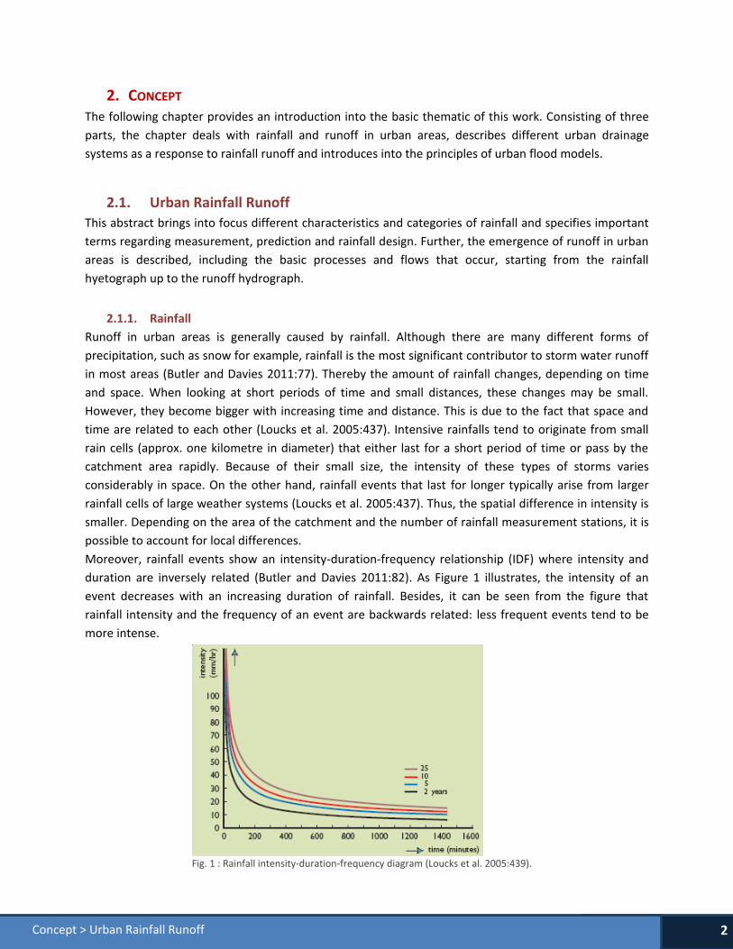
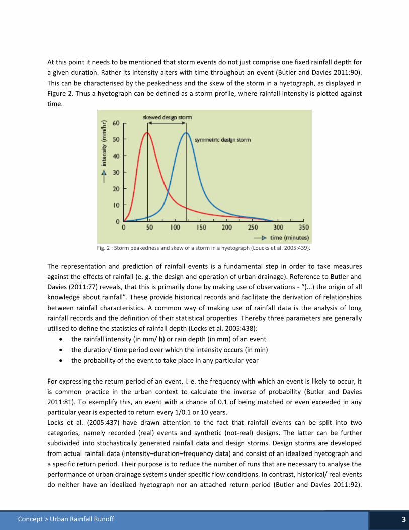
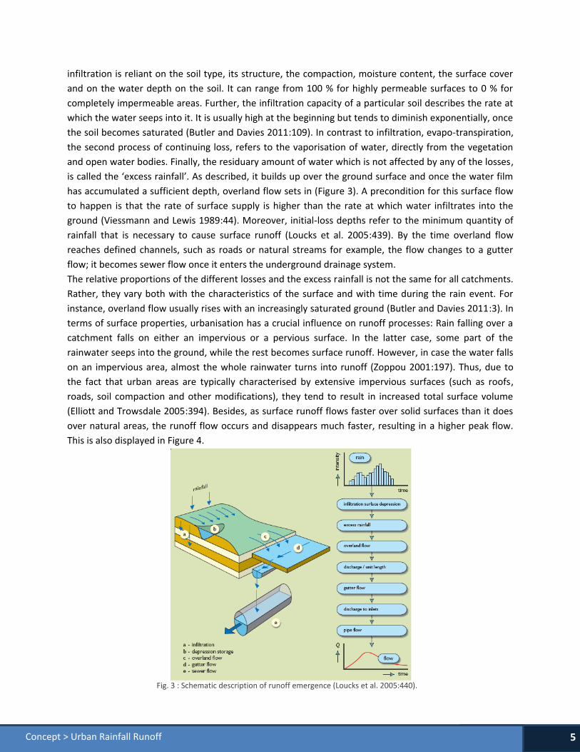
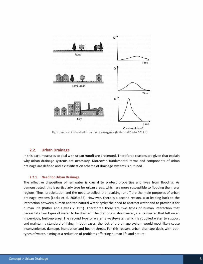
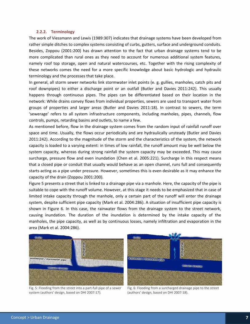
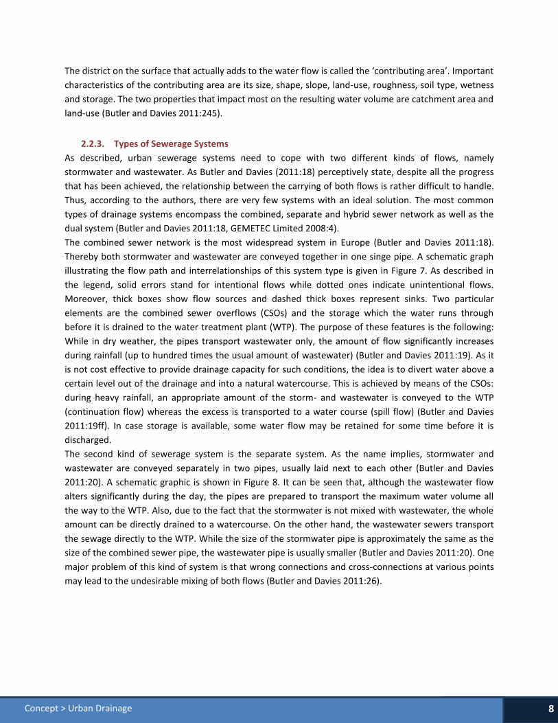
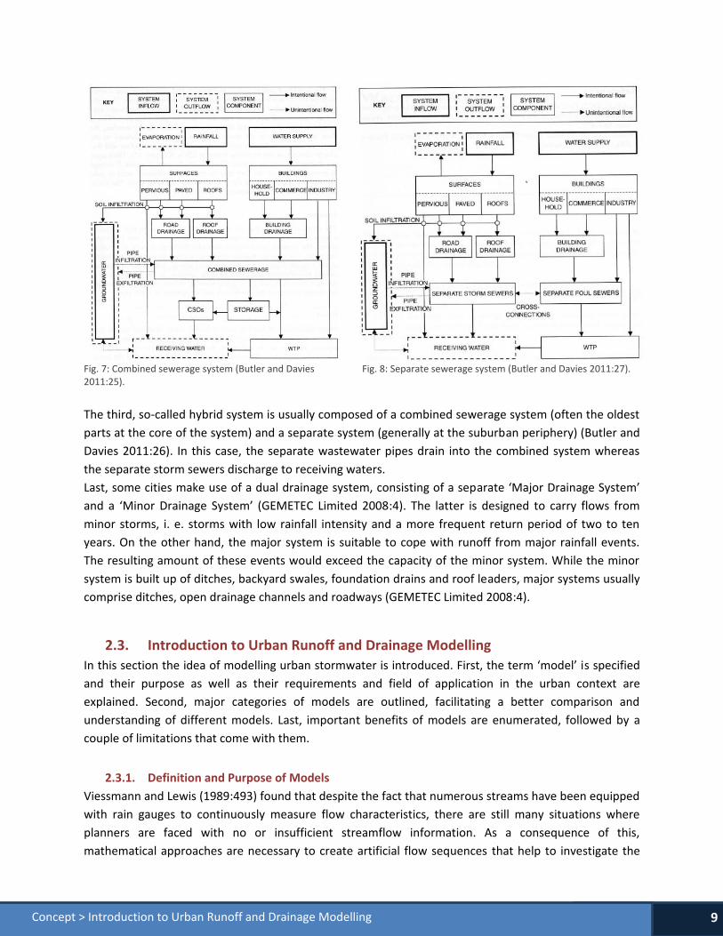
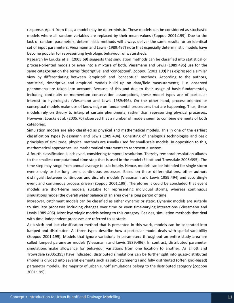
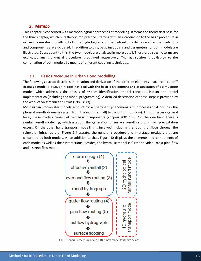
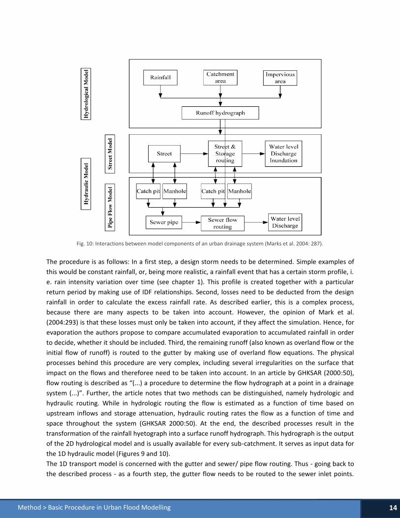
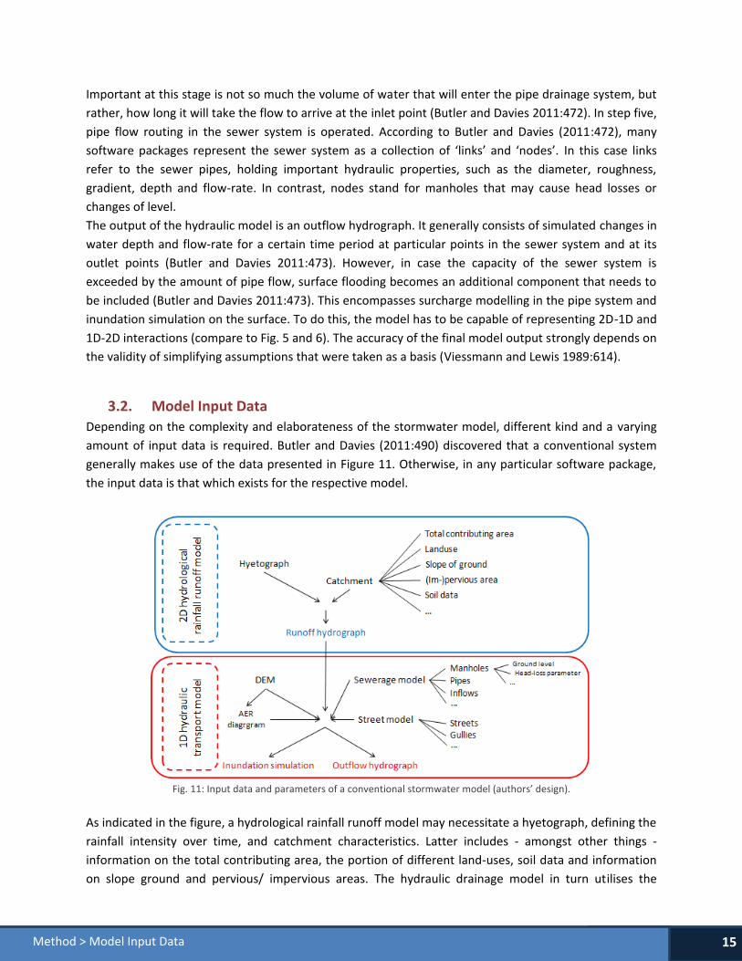
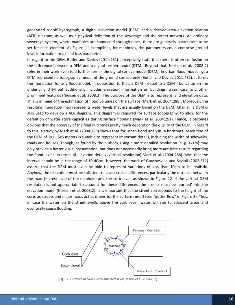
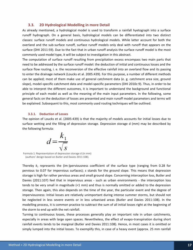
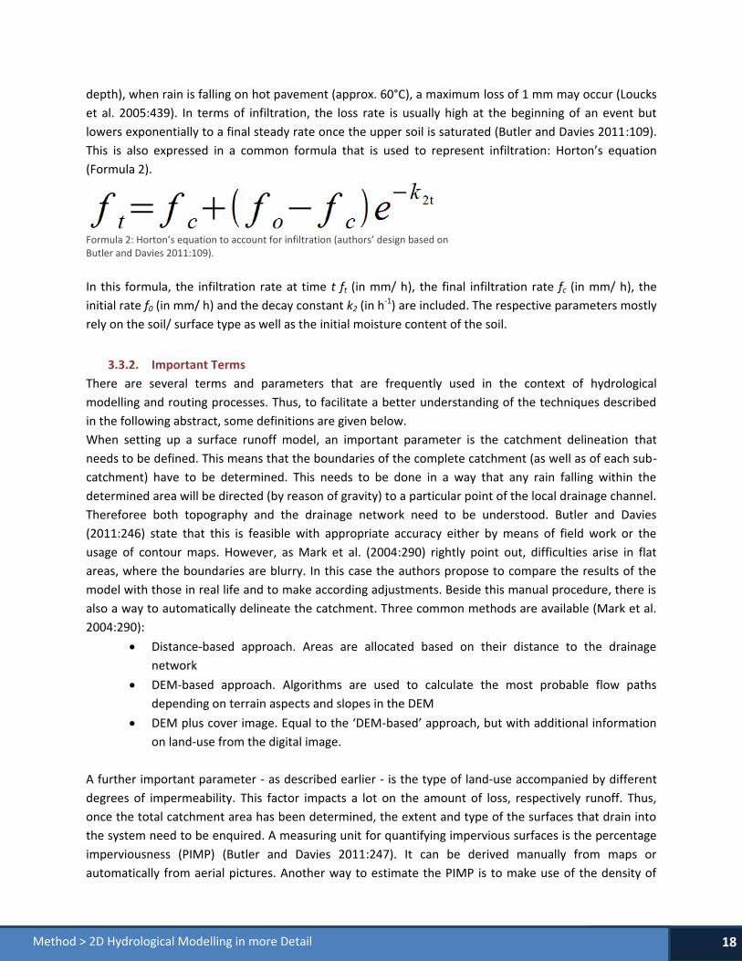
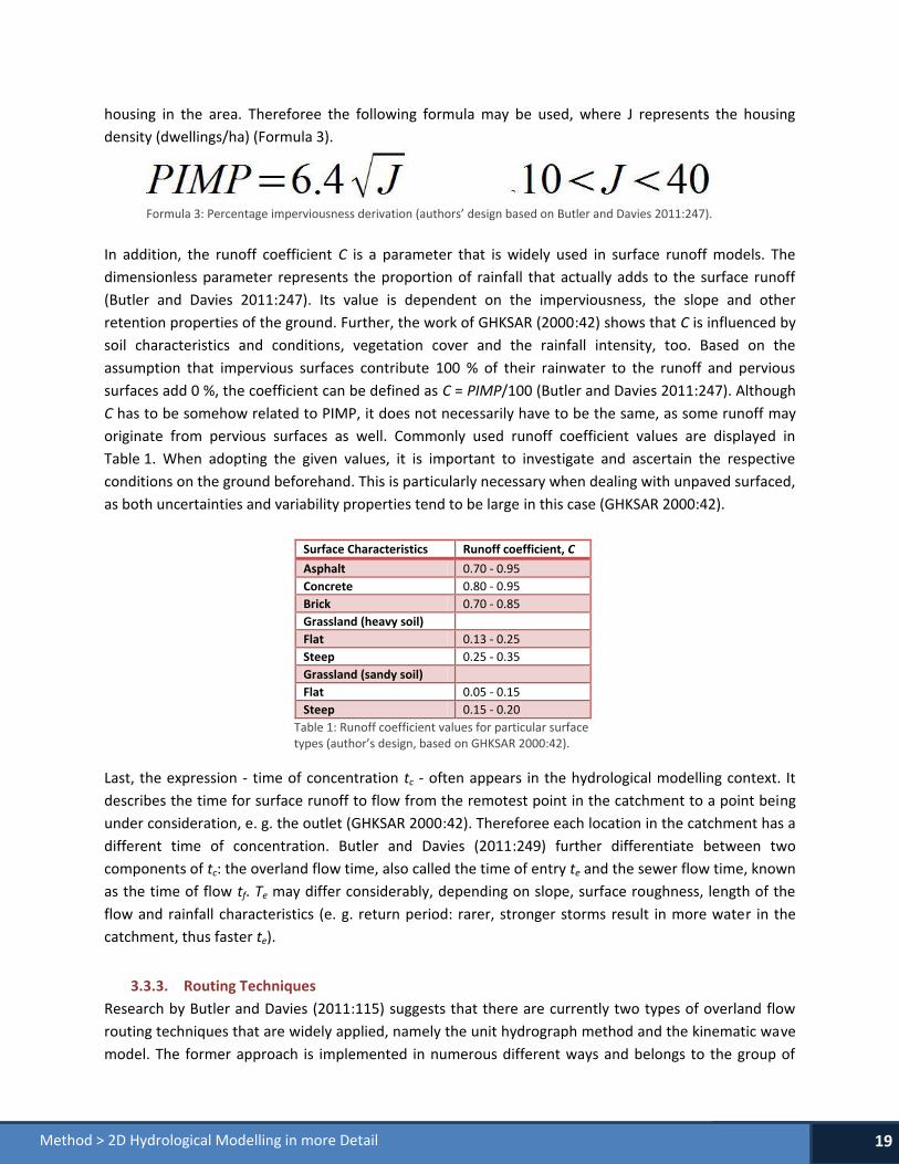
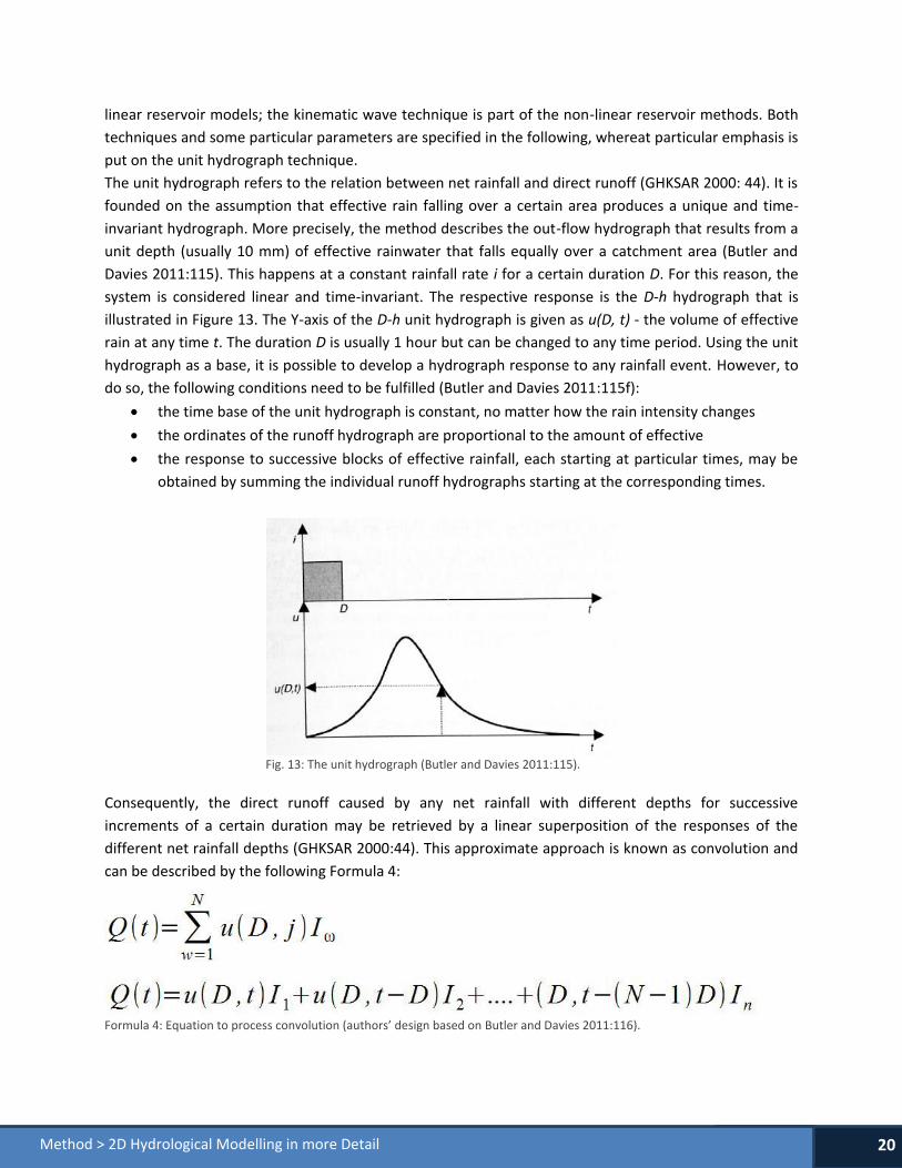
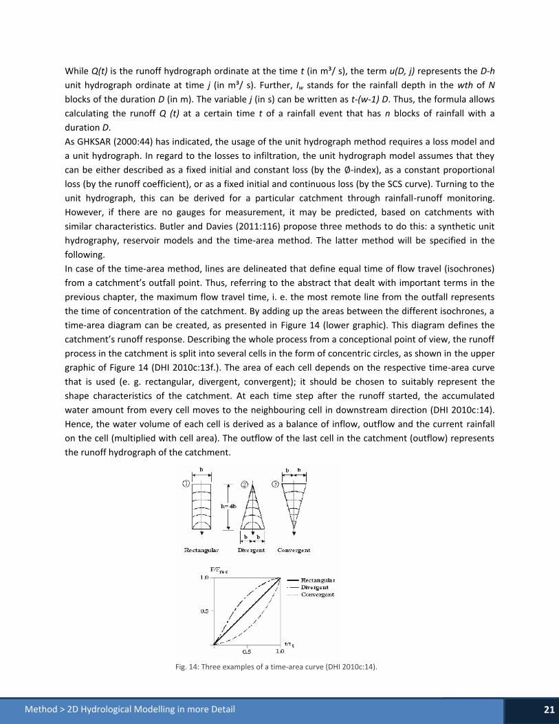
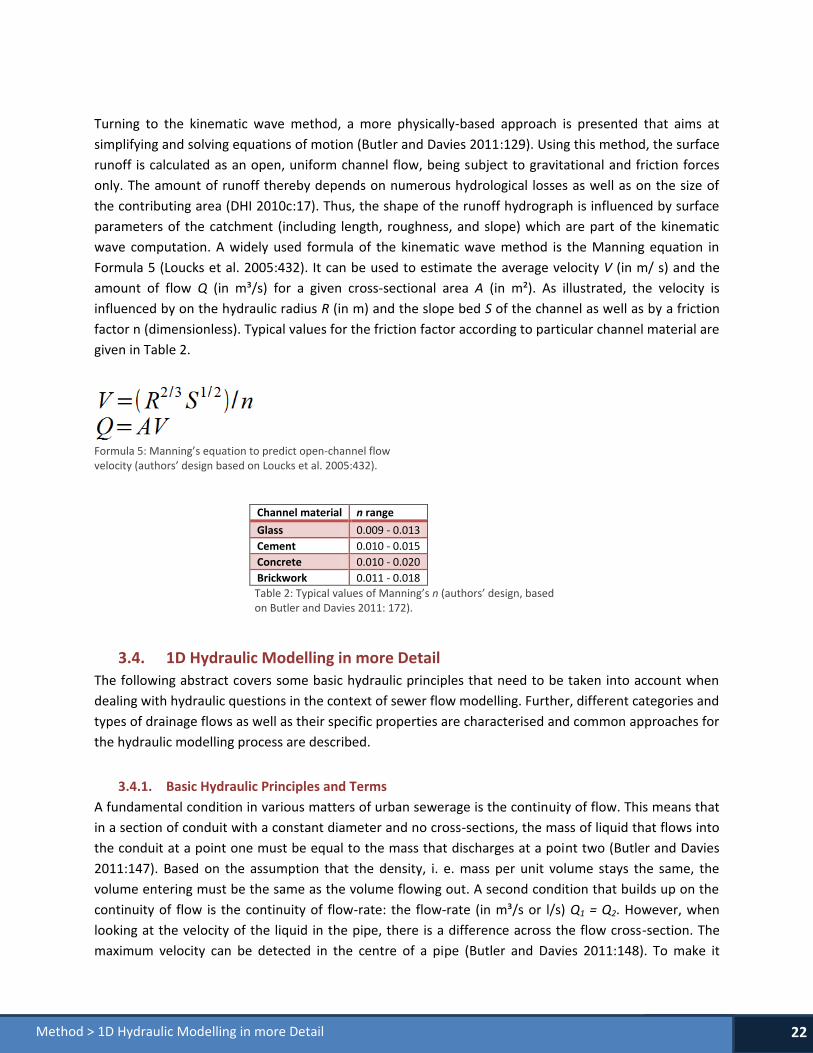
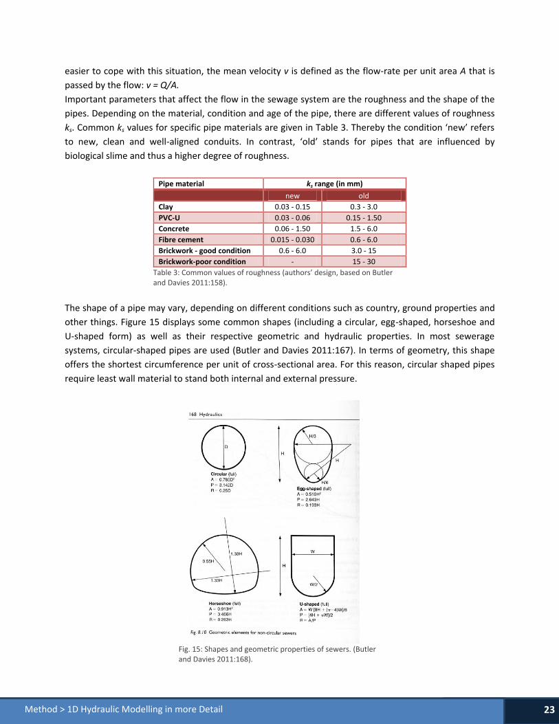
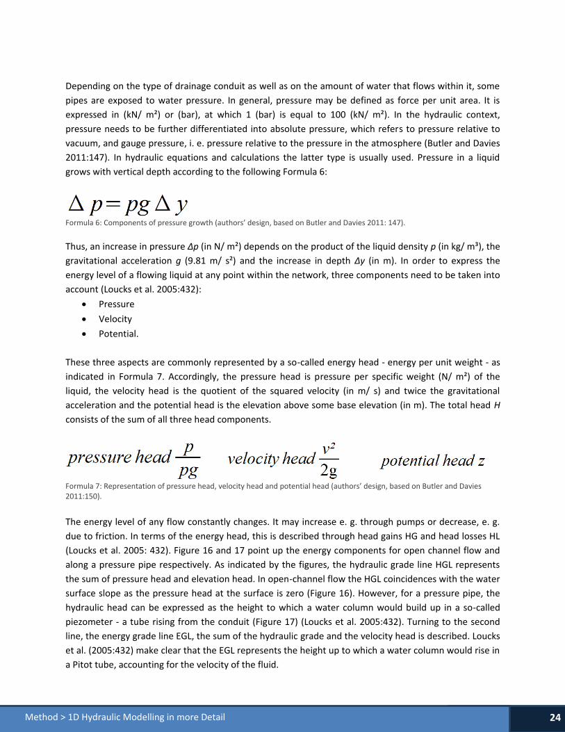
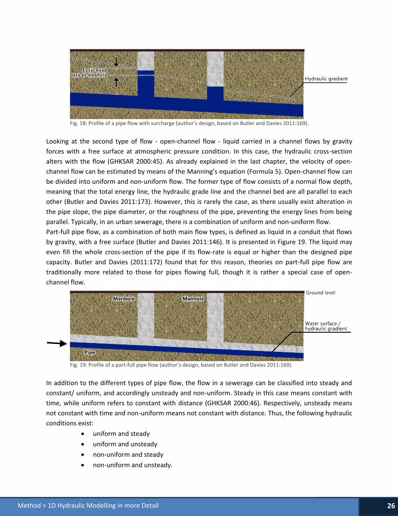
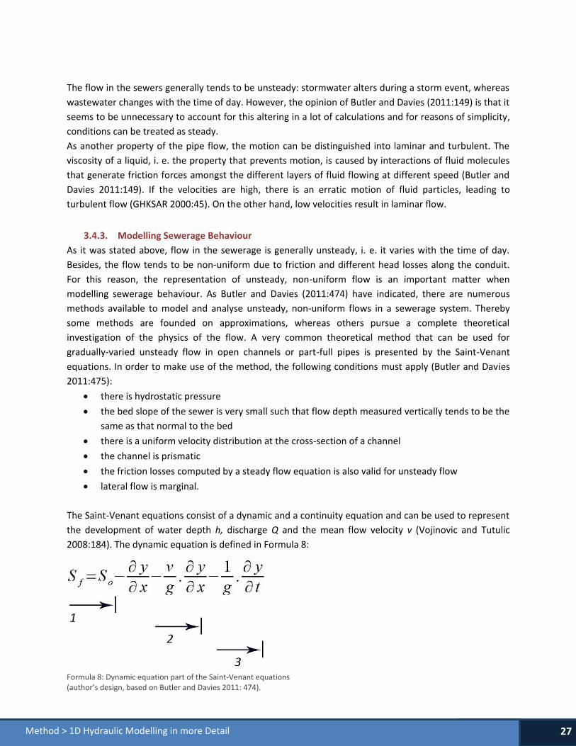
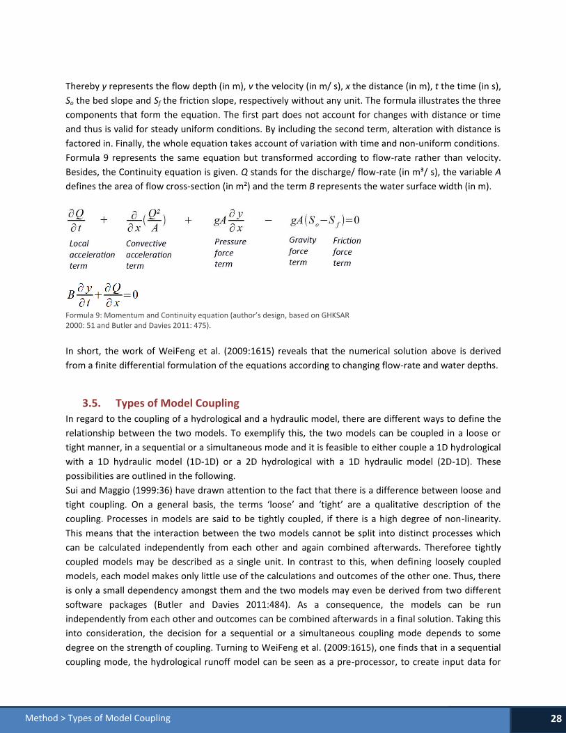
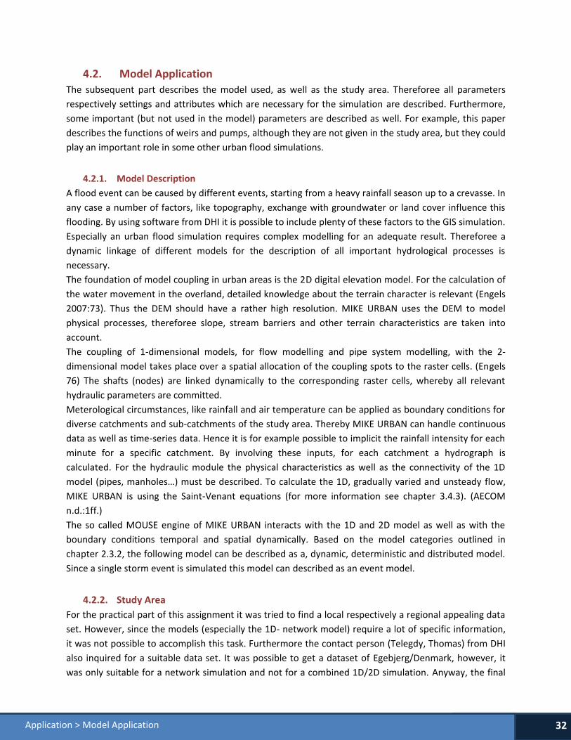
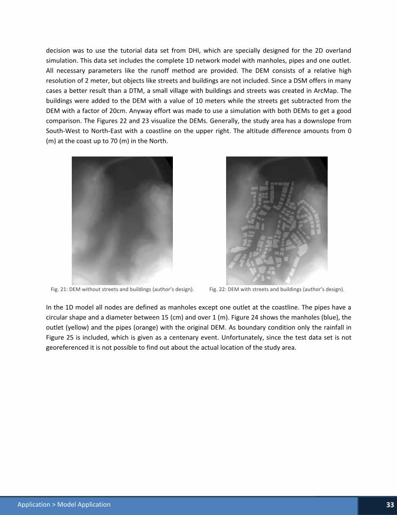
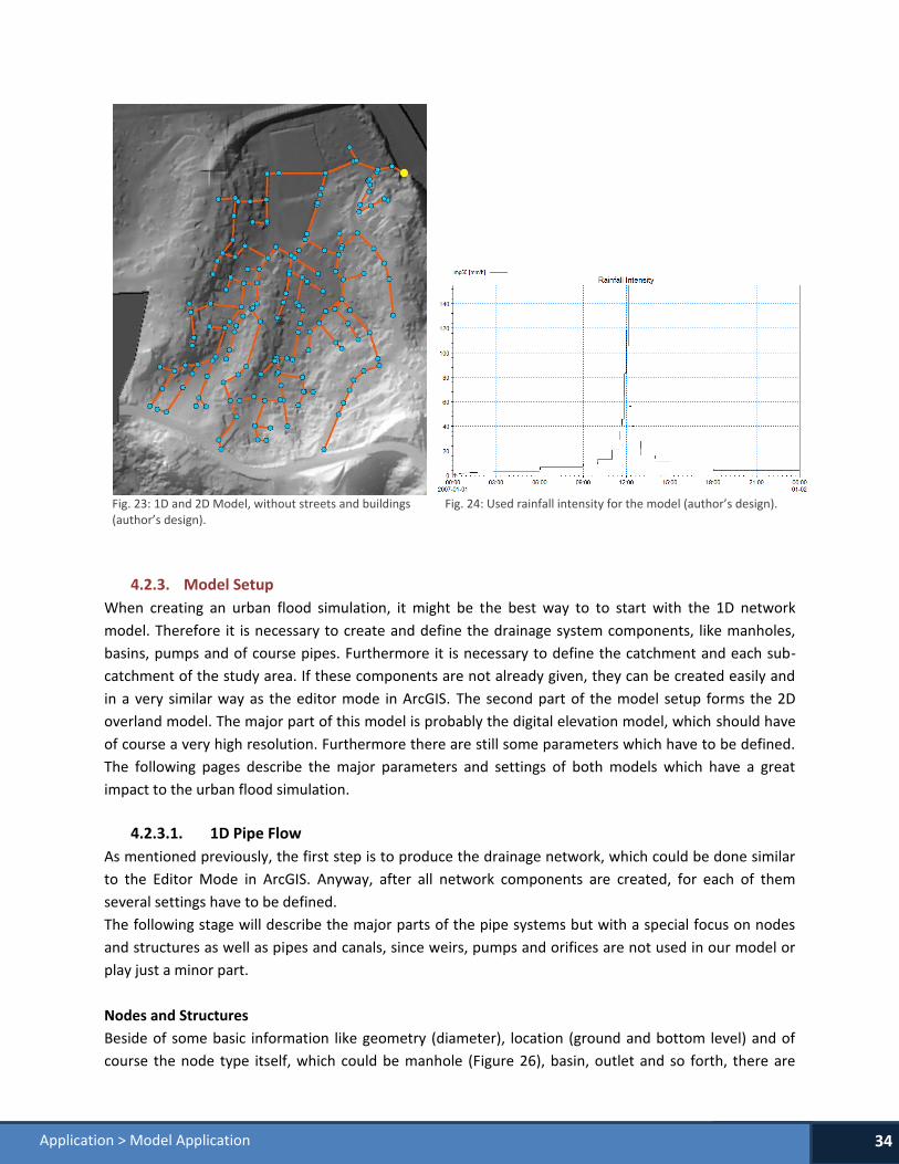
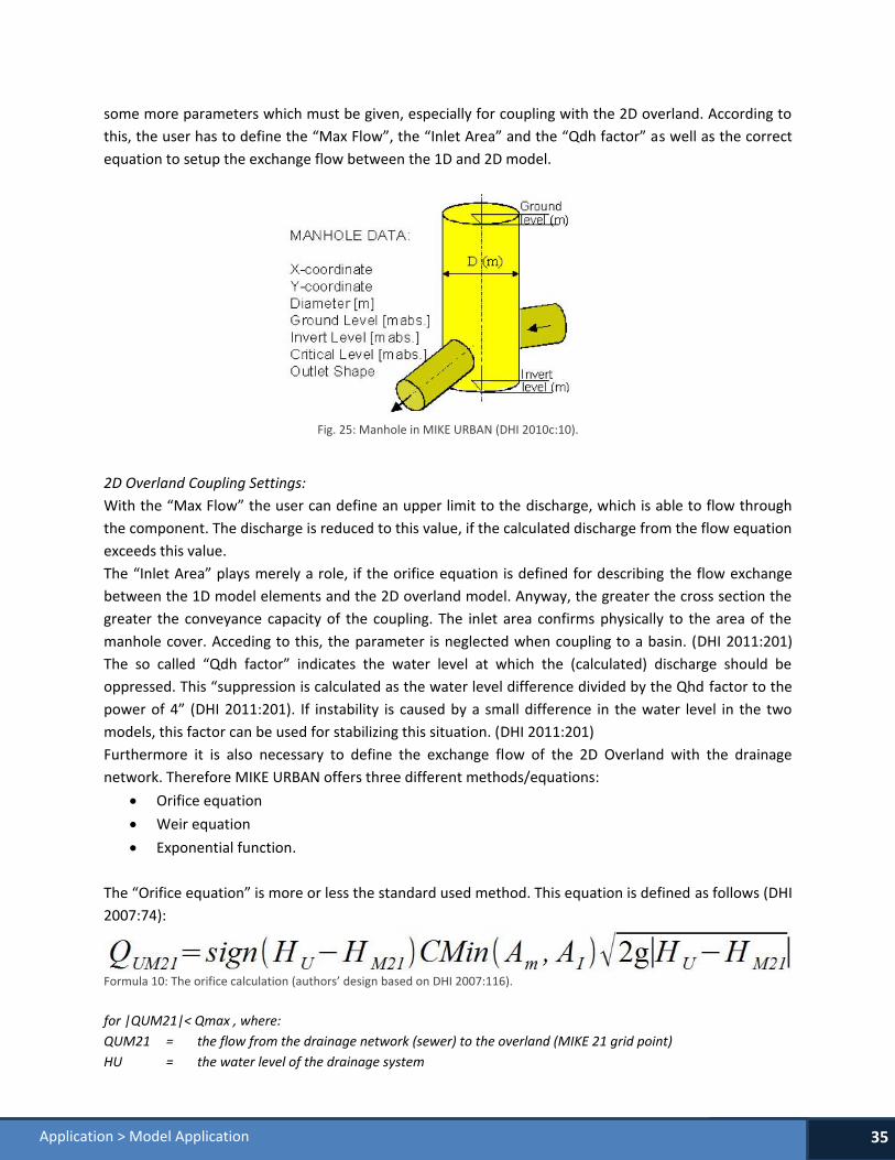
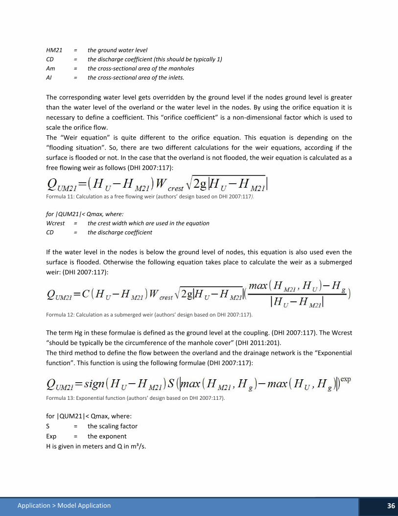
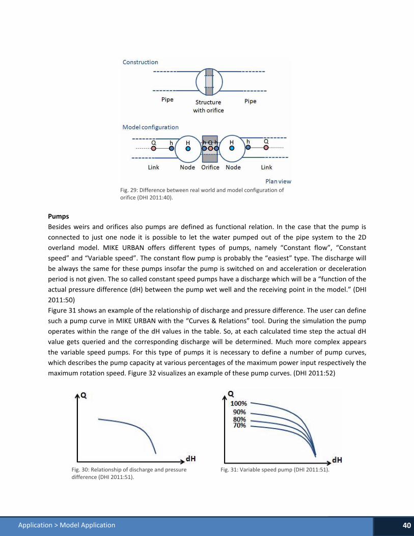
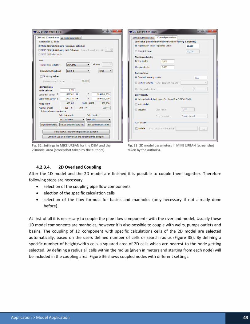
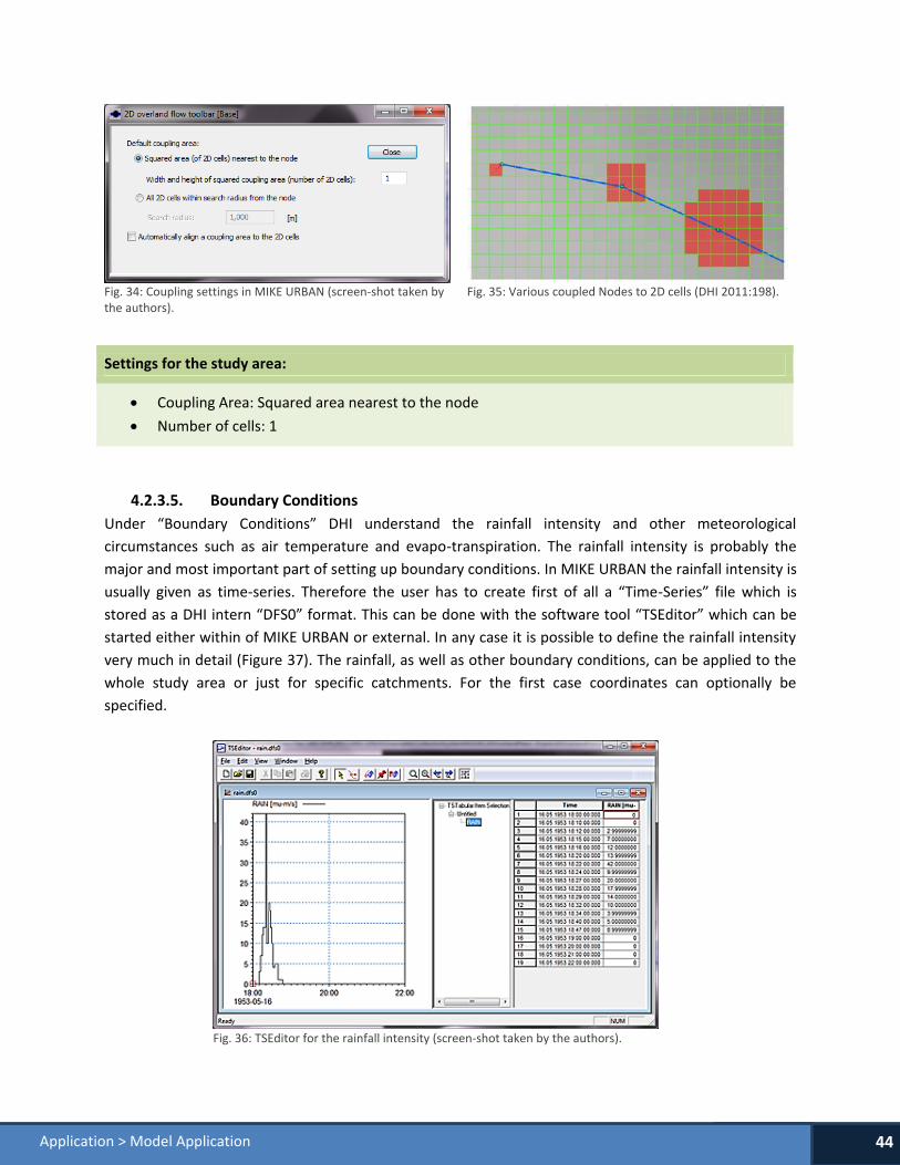
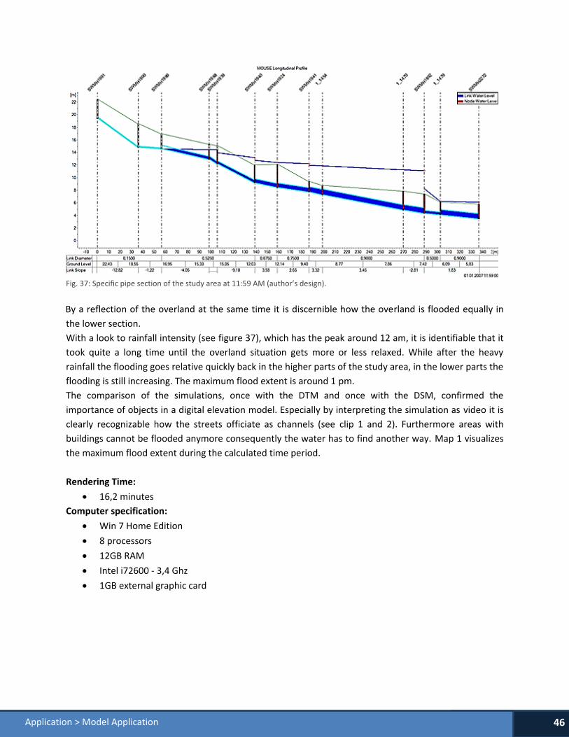
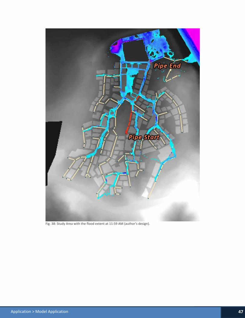
49
Application gt Coupling with Other Software
44 Coupling with Other Software
MIKE URBAN can handle data formats from different software producers Especially the import of
network data is supported while the export of results and models is provided only in minimal way
Following data formats can be amongst others imported for network data (Telegdy 2012)
AutoCAD (dwg dfx)
ESRI (Shapefiles GeoDataBase)
Excel-Spreadsheet
Text-Files (txt csv tab)
XML
MapInfo
Since MIKE URBAN store data usually in File-Based-Geodatabase respectively in Personal-Geodatabase
software products like ArcMap can access to these data However this is only possible if MIKE URBAN is
installed on the PC otherwise the freely available extension ldquoMIKE Urban Class Extensionrdquo is necessary
The DHI proprietary data format ldquodfs2rdquo for raster files can be opened end edited with diverse software
products from ESRI However it is necessary to have a MIKE URBAN license on the computer otherwise
the ESRI software is not able to open this format
45 Discussion
For both the 1D and the 2D model it is possible to set up an environment that takes account for a lot of
detailed information Also there is the opportunity to define methods and formulae for example in
regard to rainfall runoff that build up on pre-defined parameters and can be changed according to
preferable adjustments However the wide range of parameters also comes along with some drawbacks
regarding the complexity of the models Thus it is necessary that the model user possesses a well-
founded knowledge about both the software and the hydrologicalhydraulic processes that take place in
the background Especially for non-hydrologist engineers some parameters methods and formulae are
rather difficult to understand and to deal with Moreover it takes quite some time to get to know to how
the feature-rich software needs to be handled Thus especially the installation and first use of the
software tended to be frustrating It took a number of computers and installations until the software
finally run and a model was set up The documentation in form of manuals and tutorials was quite
helpful and comprehensive in this respect Besides a contact person responsible for MIKE URBAN (Mr T
Telegdy) was a great help
The reliability of the final simulation results depend more on the qualifications experience and care of
the analyst as well as the disposability of suitable data than on the software respectively the model itself
(Russ 1999 cited in Butler and Davies 2011494) Furthermore also the available data and the model
complexity itself play a major role in the simulation As Butler and Davies (2011) visualise in Figure 39
the coherence of the data availability and the model complexity influence the accuracy of the prediction
in an essential way For example low model complexity with high data availability might result into low
prediction accuracy On the other hand also a high model complexity combined with high data
availability is not the optional solution since the possibility that the available data might include some
deficiencies Therefore a complex model with a minimum of data might results in the most accurate
prediction Anyway for a specific level of model complexity there is an optimum level of data availability
50
Application gt Discussion
(for example the dotted line for high model complexity and the dashed line for a simplified model) as
well as the other way around (solid line) This means that the increasing of model complexity
respectively data availability leads to improve the predictive performance but only up to a certain level
(Buttler and Davies 2011493)
Fig 39 Coherence of data availability and model complexity (Butler and Davies 2011496)
To sum up the usage of MIKE URBAN and MIKE FLOOD is for geoinformatic students only suitable to a
up to a certain extent since the complexity of the software and the necessary appreciation of
hydrological and hydraulic givens are rather demanding Nevertheless the software is for flood modelling
and especially for an urban pipe flow evaluation very useful and commendable With some practical
work in MIKE URBAN and a good comprehension of the concepts and methods the software from DHI
can also be used by geoinformatics engineers
51
Application gt
Map 1 Maximum flood extent by using the DSM (authorsrsquo design)
52
Conclusion gt
5 CONCLUSION This paper discussed the theory and the different methods of urban flood modelling Furthermore also
the concept basics of rainfall runoff and urban drainage have been outlined For the practical part of this
work a method coupling a 1D ldquoMIKE-MOUSErdquo model and 2D ldquoMIKE-21rdquo model was used to simulate an
urban storm water event
The method of combining hydraulic and hydrological mechanism is useful for water management and
overland flow analysis in urban areas Moreover with the outcome of the simulation flood risk areas can
be identified respectively defined Thus strategies for minimizing repercussions of heavy rain fall events
can be elaborated by experts Since it is possible to include real-time data like weather radar information
and to do some real-time modifications (for example opening and closing pumps) during the simulation
the method can also be used as an early-warning system and give the agencies the opportunity to
intervene timely into the urban sewer system The complexity of a dynamic urban flood simulation by
coupling a 1D with a 2D model is great For both models it is inevitable that the analyst understands a
range of parameters and necessary settings otherwise the simulation might result in error prone
outcomes
With the software from DHI the user has the great possibility to do a dynamic 1D-2D simulation Once
the structure of the models is given it is possible to run the simulation very quickly Also changes can be
applied in an easy and fast manner However it is still necessary that the analyst understand the
essential factors as well as the meaning of the formulae and the parameters which must be defined The
link to ESRIs ArcGIS is quite good while the connectivity to other GIS software could be improved
To sum up both MIKE URABN and MIKE FLOOD seem to be very sophisticated and holistic tools This
brings advantages on the one hand but also drawbacks on the other In order to make use of all provided
product features and to gain sensible results from the application a high degree of experience and
background knowledge are necessary However taking into account the outcomes that the software
provides a solid base can be derived to be used for further investigations
ii
References gt
REFERENCES AECOM (n d) Hydrologic and Hydraulic Modeling
lthttpwwwcityofnewportcomdepartmentsutilitiespollution_controlphase240_Hydro_Hydraulic
pdfgt (last access 2012-05-25)
BUTLER D and DAVIES J (20113) Urban Drainage London Taylor amp Francis Group
CHEN A HSU M CHEN T and CHANG T (2005) An integrated inundation model for highly developed
urban areas In Water Science and Technology Vol 51 IWA Publishing 221-229
DHI (2007) MIKE FLOOD 1D-2D Modelling User Manual Available with DHI Softwaregt
DHI (2010a) MIKE 1D DHI Simulation Engine for MOUSE and MIKE 11 Reference Manual ltAvailable
with DHI Softwaregt
DHI (20103b) MOUSE Pipe Flow Reference Manual ltAvailable with DHI Softwaregt
DHI (20103c) MOUSE Runoff Reference Manual ltAvailable with DHI Softwaregt
DHI (2011) MIKE URBAN Collection System MIKE URBAN CS - MOUSE User Gide ltAvailable with DHI
Softwaregt
DHI (2012a) Urban coastal and riverine flooding
lthttpwwwdhisoftwarecomProductsWaterResourcesMIKEFLOODaspxgt (last access 10072012)
DHI (2012b) Welcome to the DHI Group lthttpwwwdhigroupcomgt (last access 23052012)
DHI (2012c) MIKE URBAN - modelling water in the city
lthttpwwwdhisoftwarecomProductsCitiesMIKEURBANaspxgt (last access 2012-06-20)
ELLIOTT A and TROWSDALE S (2005) A review of models for low impact urban stormwater drainage In
Environmental Modelling amp Software Vol 22 No 3 394-405
ENGELS R (2007) MIKE URBAN FLOOD Modellkopplung von Kanalnetzmodell und 2D
Oberflaumlchenmodell 1 Aachener Softwaretag in der Wasserwirtschaft
GEMETEC LIMITED (2008) Best Practices Assessment Stormwater Management Final Report Fredericton
lthttpwwwnbeianbcapdfStorm20Water20Management20Best20Practices20Assessmentp
dfgt (last access 2012-05-05)
GOURBESVILLE P SAVIOLI J (2002) Urban runoff and flooding interests and difficulties of the 2D
approach Hydroinformatics Proceedings of the Fifth International Conference on Hydroinformatics
Cardiff
GOVERNMENT OF THE HONG KONG SPECIAL ADMINISTRATIVE REGION (GHKSAR) (20003) Stormwater Drainage
Manual Planning Design and Management Hong Kong
iii
References gt
HSU M CHEN S AND CHANG T (2000) Inundation simulation for urban drainage basin with storm sewer
system In Journal of Hydrology Vol 234 No 1-2 21-37
LOUCKS D VAN BEEK E STEDINGER J DIJKMAN J and VILLARS M (2005) Water Resources Systems
Planning and Management An Introduction to Methods Models and Applications UNESCOParis
MARK O WEESAKUL S APIRUMANEKUL C AROONNET S and DJORDJEVIC S (2004) Potential and limitations
of 1D modelling of urban flooding In Journal of Hydrology Vol 299 No 3-4 284-299
NIELSEN N JENSEN L LINDE J and HALLAGER P (2008) Urban Flooding Assessment In 11th International
Conference on Urban Drainage Edinburgh
SUI D and MAGGIO R (1999) Integrating GIS with hydrological modeling practices problems and
prospects In Computers Environmnt and Urban Systems Vol 23 Pergamon 33-51
TELEGDY T (2011) MIKE URBAN lthttpwwwtelegdyatmikeurbangt (last access 20062012)
TELEGDY T (2012) Import und Export - eine Einleitung
httpwwwtelegdyatdokuwikiimport_einleitung (last access 12072012)
VIESSMANN W and LEWIS G (19893) Introduction to Hydrology Lavoisier SAS New York
VOJINOVIC Z and TUTULIC D (2009) On the use of 1D and coupled 1D-2D modelling approaches for
assessment of flood damage in urban areas In Urban Water Journal Vol 6 No 3 183-199
WEIFENG L QIUWEN C and JINGQIAO M (2009) Development of 1D and 2D coupled model to simulate
urban indundation An application to Beijing Olympic Village In Chinese Science Bulletin Vol 54 No 9
1613-1621
ZOPPOU C (2001) Review of urban storm water models Environmental Modelling amp Software Vol 16
No 3 195-231
iv
List of Figures gt
LIST OF FIGURES Fig 1 Rainfall intensity-duration-frequency diagram 2
Fig 2 Storm peakedness and skew of a storm in a hyetograph 3
Fig 3 Schematic description of runoff emergence 5
Fig 4 Impact of urbanisation on runoff emergence 6
Fig 5 Flooding from the street into a part-full pipe of a sewer system 7
Fig 6 Flooding from a surcharged drainage pipe to the street 7
Fig 7 Combined sewerage system 9
Fig 8 Separate sewerage system 9
Fig 9 General procedure of a 2D-1D runoff model 13
Fig 10 Interactions between model components of an urban drainage system 14
Fig 11 Input data and parameters of a conventional stormwater model 15
Fig 12 Distance between curb and crest leve 16
Fig 13 The unit hydrograph 20
Fig 14 Three examples of a time-area curve 21
Fig 15 Shapes and geometric properties of sewers 23
Fig 16 EGL and HGL for an open channel 25
Fig 17 EGL and HGL for a pipe flowing full 25
Fig 18 Profile of a pipe flow with surcharge 26
Fig 19 Profile of a part-full pipe flow 26
Fig 20 Overview of the modular structure 30
Fig 21 DEM without Streets and Buildings 33
Fig 22 DEM with Streets and Buildings 33
Fig 23 1D and 2D Model without streets and buildings 34
Fig 24 Used rainfall intensity for the model 34
Fig 25 Manhole in MIKE URBAN 35
Fig 26 Left ldquoEgg-Shapedrdquo Pipe Right ldquoO-Shapedrdquo Pipe 38
Fig 27 Open CRS channel 38
Fig 28 Closed CRS channel 38
Fig 29 Difference between real world and model configuration of orifice 40
Fig 30 Relationship of discharge and pressure difference 40
Fig 31 Variable speed pump 40
Fig 32 Settings in MIKE URBAN for the DEM and the 2Dmodel area 43
Fig 33 2D model parameters in MIKE URBAN 43
Fig 34 Coupling settings in MIKE URBAN 44
Fig 35 Various coupled Nodes to 2D cells 44
Fig 36 TSEditor for the rainfall intensity 44
Fig 37 Specific pipe section of the study area at 1159 AM 46
Fig 38 Study Area with the flood extent at 1159 AM 47
Fig 39 Coherence of data availability and model complexity 50
v
List of Tables gt
LIST OF TABLES Table 1 Runoff coefficient values for particular surface types 19
Table 2 Typical values of Manningrsquos n 22
Table 3 Common values of roughness 23
LIST OF FORMULAE Formula 1 Representation of depression storage d (in mm) 17
Formula 2 Hortonrsquos equation to account for infiltration 18
Formula 3 Percentage imperviousness derivation 19
Formula 4 Equation to process convolution 20
Formula 5 Manningrsquos equation to predict open-channel flow velocity 22
Formula 6 Components of pressure growth 24
Formula 7 Representation of pressure head velocity head and potential head 24
Formula 8 Dynamic equation part of the Saint-Venant equations 27
Formula 9 Momentum and Continuity equation 28
Formula 10 The orifice calculation 35
Formula 11 Calculation as a free flowing weir 36
Formula 12 Calculation as a submerged weir 36
Formula 13 Exponential function 36
- DeckblattAna
- cadus_poetsch_seminar-paperpdf
-
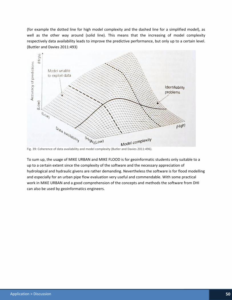
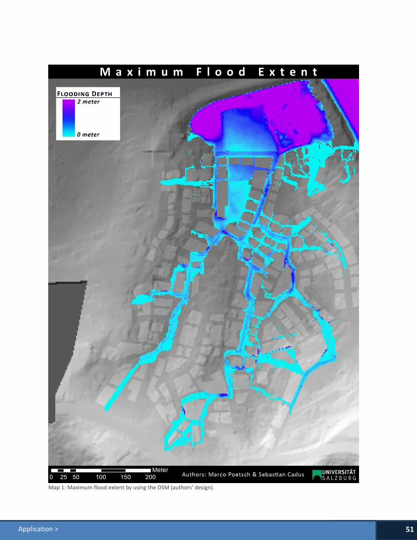