modelling and estimating the forward price curve … · modelling and estimating the forward price...

MODELLING AND ESTIMATING THE FORWARD PRICE

CURVE IN THE ENERGY MARKET

CARL CHIARELLA⋆, LES CLEWLOW† AND BODA KANG♯

Abstract. The stochastic or random nature of commodity prices plays

a central role in models for valuing financial contingent claims on com-

modities. In this paper, by enhancing a multi factor framework which

is consistent not only with the market observable forward price curve

but also the volatilities and correlations of forward prices, we propose a

two factor stochastic volatility model for the evolution of the gas forward

curve. The volatility is stochastic due to a hidden Markov Chain that

causes it to switch between “on peak” and “off peak” states. Based on

the structure functional forms for the volatility, we propose and imple-

ment the Markov Chain Monte Carlo (MCMC) method to estimate the

parameters of the forward curve model. Applications to simulated data

indicate that the proposed algorithm is able to accommodate more gen-

eral features, such as regime switching and seasonality. Applications to

the market gas forward data shows that the MCMC approach provides

stable estimates.

1. Introduction

The stochastic or random nature of commodity prices plays a central role

in models for valuing financial contingent claims on commodities, and in

procedures for evaluating investments to extract or produce the commodity.

There are currently two approaches to modelling forward price dynamics in

the literature. The first starts from a stochastic representation of the energy

spot asset and other key variables, such as the convenience yield on the asset

and interest rates (see for example Gibson & Schwartz (1990) and Schwartz

(1997)), and derives the prices of energy contingent claims consistent with

⋆ [email protected]; School of Finance and Economics, University of Technology,Sydney, Australia.† [email protected]; Lacima Group, Sydney, Australia.♯ Corresponding author: [email protected]; School of Finance and Economics, Uni-versity of Technology, Sydney, PO Box 123, Broadway, NSW 2007, Australia.

1

2 CARL CHIARELLA, LES CLEWLOW AND BODA KANG

the spot process. However, one of the problems in implementing these models

is that often the state variables are unobservable - even the spot price is hard

to obtain, with the problems being exacerbated if the convenience yield has

to be jointly estimated.

The second stream of literature models the evolution of the forward curve.

Forward contracts are widely traded on many exchanges with prices easily

observed - often the nearest maturity forward price is used as a proxy for the

spot price with longer dated contracts used to imply the convenience yield.

Clewlow & Strickland (1999a) work in this second stream, simultaneously

modelling the evolution of the entire forward curve conditional on the initially

observed forward curve and as such define a unified approach to the pricing

and risk management of a portfolio of energy derivative positions.

These authors go on to develop a single-factor modelling framework which is

consistent with market observable forward prices and volatilities and which

leads to analytical pricing formulae for standard options, caps, floors, collars

and convenient numerical schemes for swaptions. They also show how Amer-

ican style and exotic energy derivatives can be priced using trinomial trees

which are constructed to be consistent with the forward curve and volatility

structure.

However single-factor forward curve models leave very little room for complex

movements of the forward price curve due to an underlying assumption of

perfect correlation between forward prices of different maturities. This is

inherently unrealistic, and becomes a critical flaw when the derivative in

question depends on the relative values of points at different maturities along

the forward price curve. Another shortcoming of the single-factor model of

the forward price curve manifests itself in pricing long-term contracts on the

spot price.

Clewlow & Strickland (1999b) develop a general framework with a multi-

factor model for the risk management of energy derivatives. This framework

is designed to be consistent not only with the market observable forward price

curve but also the volatilities and correlations of forward prices. Breslin,

Clewlow, Kwok & Strickland (2008) further generalize this framework to

accommodate a more general multi-factor, multi-commodity (MFMC) model

and also describe a process for estimating parameters from historical data.

MODELLING AND ESTIMATING THE FORWARD PRICE CURVE 3

There has been a great deal of fruitful research on the models of the interest

rate term structure. Since the forward price curve shares similar patterns with

forward interest rate dynamics, in particular the Heath, Jarrow & Morton

(1992) (HJM) model, many of these ideas could potentially work in modelling

forward energy prices. The instantaneous forward price volatility is not di-

rectly observable. However the observed implied volatility (obtained from

the prices of various derivative contracts) is closely related to it and indicates

that the market is also changing its belief about the instantaneous volatilities

discontinuously. In deterministic volatility HJM models, the volatility curve

is fixed and the volatility of a specific forward rate can change deterministi-

cally only with maturity. In order to properly describe the actual evolution

of the volatility curve, one needs a process consisting of both deterministic

factors and random factors. The drawback of diffusion models is that they

cannot generate sudden and sufficiently large shifts of the volatility curve.

If one augments that feature by adding traditional type jump processes, for

example Poisson jumps, one finds that the frequency of the jumps is too large

while the magnitude of the jumps is too small.

It seems that the class of piecewise-deterministic processes provide an ap-

propriate framework for modelling the dynamics of the term structure of

volatilities since they allow volatility to follow an almost deterministic pro-

cess between two random jump times. Davis (1984) claims that this class

covers almost all important non-diffusion applications. The simplest process

in this class is the continuous-time homogeneous Markov chain with a fi-

nite number of jump times. Modelling with such a process approximates the

actual jumps in volatility with jumps over a finite set of values but allows

the well-developed stochastic calculus for continuous Markov chains (Elliott,

Aggoun & Moore (1995) and Aggoun & Elliott (2005)) to be used.

In energy markets, forward contracts are widely traded on many exchanges

with prices easily observed - often the nearest maturity forward price is used

as a proxy for the spot price with longer dated contracts used to imply the

convenience yield. Two volatility functions are proposed to model the gas

forward curve in this paper. Both volatility functions contain a common

seasonality adjustment term, but one volatility function is declining with

increasing maturity to a constant; another volatility function captures the


overall tilting of the forward curve where the short maturity contracts move

in the opposite direction to the longer maturity contracts. We allow the

parameters (including the spot volatilities and the attenuation parameters)

of the volatility functions to take different values in different states of the

world. The dynamics of the “states of the world”, for example an “on-peak”

or “off-peak” time for gas, or a “good” or “bad” economic environment are

represented by a Markov Chain. The evolution of the two volatility functions

depend on the transition of the Markov Chain.

The rest of the paper is organized as follows. A two factor regime switching

model for the gas forward price curve is discussed in Section 2. In Section 3 a

Markov Chain Monte Carlo approach including several detailed algorithms is

analysed and implemented to estimate the parameters in the model. A num-

ber of numerical examples and the calibration results from the real market

data are discussed in Section 4. Finally a conclusion is drawn in Section 5.

2. Two-factor regime switching forward price curve model

The single-factor models proposed in Clewlow & Strickland (1999a) have a

wide range of applicability in energy valuation and risk management, and are

relatively simple to understand and parameterise. While these models can

capture much of the dynamics of actual life processes in many circumstances,

by definition they only use a small amount of the potential information avail-

able from the market. In particular, one major drawback of single-factor

models is that they imply that instantaneous changes in forward prices at all

maturities are perfectly correlated. Increasingly, energy risk practitioners are

attracted to modelling frameworks that avoid such simplifications. Where

enough data is available, a more general multi-factor model can be used to

capture extra information about the price dynamics, and this is the modelling

framework that we concentrate on here. It is also relatively straightforward

to extend such a multi-factor model to incorporate multiple commodities.

Following the spirit of both Clewlow & Strickland (1999b) and Breslin et al.

(2008) and the idea of the piecewise deterministic processes discussed in the

previous section, rather than a general form of the volatility functions in the

multi-factor model, we propose a two factor model in which we specify the ex-

plicit form of the volatility function. Benth & Koekebakker (2008) compared


several different volatility dynamics of the forward curve models under the

HJM framework. In this paper, incorporating both the volatility functional

form of these latter authors and the Markov switching of the coefficients, we

propose the following two-factor regime switching model for the gas forward

curve:dF (t, T )

F (t, T )= σ1(t, T )dW1(t) + σ2(t, T )dW2(t), (1)

with

σ1(t, T ) = < σ1, Xt > c(t)(

e−<α1,Xt>(T−t) · (1 − σl1) + σl1

)

,

σ2(t, T ) = < σ2, Xt > c(t)(

σl2 − e−<α2,Xt>(T−t))

,

c(t) = c +

J∑

j=1

(dj(1 + sin(fj + 2πjt))) ,

where:

• F (t, T ) is the price of the gas forward at time t with a maturity at

time T .

• Xt is a finite state Markov chain with state space S = {e1, e2, · · · , eN}

where ei is a vector with length N and 1 at the i−th position and 0

elsewhere, that is

ei = (0, . . . , 0, 1, 0, . . . , 0)′ ∈ RN .

• P = (pij)N×N is the transition probability matrix of the Markov Chain

Xt. For all i = 1, . . . , N, j = 1, . . . , N, pij is the conditional probabil-

ity that the Markov Chain Xt transit from state ei at time t to state

ej at time t+ 1, that is,

pij = Pr(Xt+1 = ej |Xt = ei).

• For i = 1, 2,

σi = (σi1, σi2, · · · , σiN ), αi = (αi1, αi2, · · · , αiN),

are the different values of the volatilities and attenuation parameters

which evolve following the rule of the Markov Chain Xt.


• < ·, · > denotes the scalar product in RN , if u = (u1, · · · , uN) then

< u,Xt >=

N∑

i=1

uiI(Xt=ei);

where I(Xt=ei) is the indicator function:

I(Xt=ei) =

{

1 Xt = ei

0 otherwise.

• σl1 and σl2 describe some features of the long run volatility;

• c(t) - the seasonal part which is modelled as a truncated Fourier series;

• W1(t) and W2(t) are independent Brownian motions.

In the above model, both volatility functions contain a common seasonality

adjustment term c(t), but σ1(t, T ) is declining with increasing maturity to a

constant and σ2(t, T ) captures the overall tilting of the forward curve where

the short maturity contracts move in the opposite direction to the longer

maturity contracts.

In the above model, some parameters of the proposed volatility function will

change from one value to another depending on the state of the world or the

change of the market structure. The transition of the state is characterized

by a finite state Markov Chain. The element of the transition probability

matrix P will form part of the parameter set to be estimated.

3. Estimation algorithms and Implementations

Hahn, Fruhwirth-Schnatter & Sass (2007) use a Bayesian approach to esti-

mate a Markov Switching Model (MSM). They derive a Markov Chain Monte

Carlo Method (MCMC) for the MSM which yields better results than the

corresponding EM algorithm.

Based on the structure of our volatility functional forms, we propose and im-

plement the MCMC to estimate the parameters of the above forward curve

model. Applications to simulated data indicate that the proposed algorithm

is able to accommodate more general features, such as regime switching, sea-

sonality, certain functional form of forward volatility functions. Applications

to the market gas forward data shows that the MCMC approach provides

stable estimates.


In this section, we describe an algorithm to estimate the set of parameters

θ = {σi, αi, σli(i = 1, 2), c, dj, fj, (j = 1, 2, . . . , J)}

and the elements of the transition probability matrix P given the forward

prices at fixed observation times ∆t, 2∆t, . . . ,M∆t = t assuming that the

state process can jump only at the discrete observation times.

3.1. Data transformation. For any maturity time T , we observe forward

prices F (k∆t, T ), k = 1, . . . ,M from the market. Setting yT = {yt,T , t ≥ 0},

we rewrite the forward dynamics (1) in discrete time as

yt,T := log(F (t+ ∆t, T )) − log(F (t, T ))

= −1

2

2∑

i=1

σi(t, T )2∆t+2∑

i=1

σi(t, T )∆Wi(t).

Apparently, given all parameters and the state of the Markov Chain at each

time, the difference of the log of forward price, namely yt,T is normally dis-

tributed and the random variables are independent for different t. Hence,

yt,T is normal distributed with a mean of µt,T = −12

∑2i=1 σi(t, T )2∆t and

standard deviation σt,T =√

∆t∑2

i=1 σi(t, T )2.

3.2. Prior Distributions. Prior distributions have to be chosen for θ and

X0.

Assumption 3.1. Assume that θ = {σi, αi, σli(i = 1, 2), c, dj, fj , (j = 1, 2, . . . , J)}, P

and X0 are independent, that is

Pr(θ, P,X0) = Pr(P )Π2i=1(Pr(σi)·Pr(αi)·Pr(σli))Pr(c)ΠJ

j=1(Pr(dj)Pr(fj))Pr(X0).

In addition to Assumption 3.1 we further assume that, for l = 1, . . . , N and

i = 1, 2, j = 1, . . . , J :

• The rows Pl of P are assumed to be independent and to follow a

Dirichlet distribution

Pl ∼ D(gl1, · · · , glN).

• The priors of σs and αs are

σil ∼ U(aσil, b

σil), αil ∼ U(aα

il, bαil).


• The priors of σli are

σli ∼ U(0, 1).

• The priors of c, d, f are

c, d, f ∼ U(ac, bc).

• The prior of the initial state of the Markov chain

X0 ∼ U({1, . . . , N}).

All parameters gl1, · · · , glN , aσil, b

σil, a

αil, b

αil, a

c, bc in the prior distributions

need to be chosen carefully before the calibrations process.

3.3. Full conditional posterior distributions. To sample from the joint

posterior distribution of {σi, αi, σli(i = 1, 2), c, dj, fj, (j = 1, 2, . . . , J)}, P and

X given the observed data yT, we partition the unknowns into three blocks

θ, P and X, and draw each of them from the appropriate conditional density.

3.3.1. Complete-data likelihood function. Given θ, P and X, the log return

process yT is independent, and the likelihood function is given by

P (yT |θ, P,X) = ΠMk=1φ(yk∆t,T , µk∆t,T , σk∆t,T ), (2)

where φ(y, µ, σ) denotes the density of a normal distribution with mean µk∆t,T

and standard deviation σk∆t,T , given here by

µt,T = −1

2

2∑

i=1

σi(t, T )2∆t, σt,T =

√

√

√

√∆t

2∑

i=1

σi(t, T )2.

3.3.2. Drift and volatility. The conditional joint distribution of the parame-

ters associated with drift and volatility is given by

Pr(θ|yT , P,X) ∝ Pr(yT |θ,X)Pr(θ).

3.3.3. State process. The prior distribution of the state process Xl∆t, l =

1, 2, . . . ,M is determined by the distribution of X0, and the transition prob-

abilities P , and is independent of θ. Therefore the full conditional posterior

is

Pr(X|yT , θ, P ) ∝ Pr(yT |θ,X)P (X|P ).


Defining Nlq =∑M

k=1 I{Xk−1=l,Xk=q},the number of transitions from state l to

q, the probability of X given P is:

Pr(X|P ) = P (X0|P )ΠMk=1Pr(Xk|Xk−1, P ) = P (X0|P )ΠN

l,q=1PNlq

lq .

By forward-filtering-backward-sampling, we update X by drawing from the

full conditional posterior Pr(X|yT , θ, P ).

3.4. Proposal distributions.

3.4.1. Drift and volatility. For the update of θ, we use the normal random

walk

θ′ = θ + rθψ, (3)

where ψ is a matrix of independent standard normal random variables and

rθ are parameters scaling the step widths. Hence, we have a Metropolis step

(see Hahn et al. (2007)) with acceptance probability αθ = min{1, αθ}, where

αθ =Pr(yT |θ

′, X)Pr(θ′)

Pr(yT |θ)P (θ).

3.4.2. Transition matrix. For the update of the transition matrix, we use the

method of sampling from a Dirichlet distribution as described in Fruhwirh-

Schnatter (2006). For each row l = 1, . . . , N of the transition matrix, the

proposal

P ′l ∼ D(gl1 +Nl1, . . . , glN +NlN),

is used. If the initial distribution of the state process Pr(X0) is independent

of P , then P ′l is a sample from the appropriate full conditional distribution,

and we obtain a Gibbs step (see Hahn et al. (2007)) with acceptance rate 1.

3.5. Algorithm. Start with some state process X0 and repeat the following

steps for k = 1, . . . , K0, . . . , K +K0.

(1) Parameter simulation conditional on the states X(k−1):

• Sample the transition matrix P (k) from the complete-data

posterior distribution p(·|X(k−1)).

• Sample the model parameters θ(k) from the complete-data

posterior p(θ|yT ,X(k−1)) (Metropolis-Hastings algorithm).

Store the actual values of all parameters as (θ(k), P (k)) .


(2) Markov Chain State simulation conditional on (θ(k), P (k)) by sam-

pling a path X of the hidden Markov chain from the conditional

posterior p(X|(θ(k), P (k)),yT ) (forward-filtering-backward-sampling).

Store the actual values of all states as X(k), increase k by one, and

return to step (1). Finally, the first K0 draws are discarded.

4. Applications

In this section, we describe some details on the implementation, then we

present numerical results of the proposed algorithms both for simulated data

and historical gas forward prices.

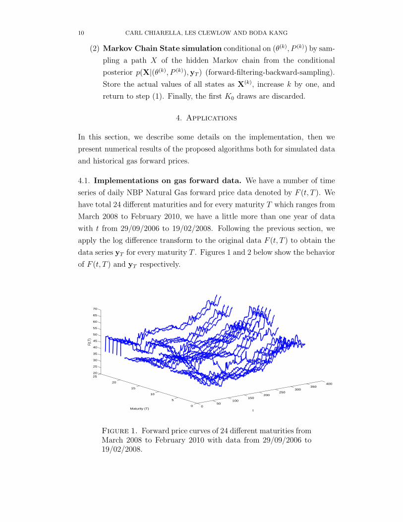
4.1. Implementations on gas forward data. We have a number of time

series of daily NBP Natural Gas forward price data denoted by F (t, T ). We

have total 24 different maturities and for every maturity T which ranges from

March 2008 to February 2010, we have a little more than one year of data

with t from 29/09/2006 to 19/02/2008. Following the previous section, we

apply the log difference transform to the original data F (t, T ) to obtain the

data series yT for every maturity T . Figures 1 and 2 below show the behavior

of F (t, T ) and yT respectively.

050

100150

200250

300350

400

0

5

10

15

20

2520

25

30

35

40

45

50

55

60

65

70

tMaturity (T)

F(t,T

)

Figure 1. Forward price curves of 24 different maturities fromMarch 2008 to February 2010 with data from 29/09/2006 to19/02/2008.


050

100150

200250

300350

400

0

5

10

15

20

25−0.15

−0.1

−0.05

0

0.05

0.1

0.15

0.2

0.25

0.3

tMaturity (T)

y t,T

Figure 2. The differences of the log of forward prices yT with24 different maturities from March 2008 to February 2010 withdata from 30/09/2006 to 19/02/2008.

We use a two-state Markov Chain in this implementation, hence we setN = 2.

4.1.1. Choosing the prior. The prior distribution should be independent of

the data and the posterior distribution. However in order to obtain a rela-

tively accurate and relevant prior distribution, we obtain some information

from both the data and the historical estimation and information about the

range of the parameters. The following priors are used in the implementation:

(1) For the transition matrix P , the vector gl· equals the prior expectation

of Pl· times a constant that determines the variance. If P 0 denotes

our prior expectation of P , we may set gl· = P 0l·cp. Then cp can be

interpreted as the number of observations of jumps out of state l in the

prior distribution. Hence, the matrix of parameters for the Dirichlet

distribution is set to

g =

(

0.64 0.36

0.16 0.84

)

· cp. (4)

where cp = 15.

(2) The priors of σs and αs (i, l = 1, 2) are

σil ∼ U(0, 1.5), αil ∼ U(0, 5).


(3) The priors of σli are

σli ∼ U(0, 1).

(4) The priors of c, d, f (J = 1) are

c, d1, f1 ∼ U(0, 1).

(5) The prior of the initial state of the Markov chain are

X0 ∼ U({1, 2}).

4.1.2. Running MCMC. To implement the Metropolis-Hastings algorithm,

the scaling factors rθ have to be selected in (3). We found that selecting

rθ around 1% to 5% of the minimal difference between two adjacent initial

values among θ worked well.

In order to use all available information about forward prices on the market,

we implemented a “randomised” algorithm to calculate the complete-data

likelihood function.

In fact, before the calibration, we choose a sequence λ = (λ1, λ2, · · · , λM)

with λk ∼ U({1, 2, · · · , 24}), k = 1, . . . ,M where λk ranges from 1 to 24

to label 24 different maturities. At each time k · ∆t in the data series, we

choose the data yt,Tjwith the maturity Tj if λk = j. Hence the complete-data

likelihood function (2) under this setting is

P (yTλ|θ, P,X) = ΠM

k=1φ(yk∆t,Tλk, µk∆t,Tλk

, σk∆t,Tλk), (5)

where φ, µ and σ have the same definition as before.

4.2. Numerical results. For a two state regime, two factors model as above,

about 150, 000 steps were run and the following is the estimates of the pa-

rameters:

• Number of States N = 2

j 1 2 j 1 2

σ1j 0.3057 0.8429 σ2j 0.4762 1.0292

α1j 2.0464 1.8932 α2j 1.1533 3.2536

• c = 0.8121, d = 0.0781, f = 0.3070

• σl1 = 0.4869, σl2 = 0.6203;


• Transition probabilities

j 1 2

1 0.8516 0.1484

2 0.7080 0.2920

which shows that with high probability the Markov chain will stay in

regime 1 most of the time but with some (low) probability will jump

from regime 1 to regime 2 occasionally.

Figure 3 shows simulations of the two volatility functions σ1(t, T ) and σ2(t, T )

and one trajectory of the Markov Chain Xt.

0 50 100 150 200 250 300 350 4000

0.5

1

T−t

σ 1(t,T)

0 50 100 150 200 250 300 350 400−0.5

0

0.5

1

T−t

σ 2(t,T)

0 50 100 150 200 250 300 350 400

1

1.5

2

t

x t

Figure 3. A simulation path of two volatility functions σ1(T−t) and σ2(T − t) as a function of (T − t); but Xt evolve forwardin time with t.

Figure 4 demonstrates the shape of two volatility functions in different regimes

after the seasonal components c(t) has been removed. Those results empha-

size that one volatility function σ1(t, T ) is declining with increasing maturity

to a constant and another volatility function σ2(t, T ) captures the overall

tilting of the forward curve where the short maturity contracts move in the

opposite direction to the longer maturity contracts.

A number of MCMC estimation procedures have been run starting from

different sets of parameters with different initial samples implemented by


0 50 100 150 200 250 300 350 4000.1

0.2

0.3

0.4

0.5

0.6

0.7

0.8

0.9

T−t

σ 1(t,T)

regime 1regime 2

0 50 100 150 200 250 300 350 400−0.4

−0.2

0

0.2

0.4

0.6

0.8

1

T−t

σ 2(t,T)

regime 1regime 2

Figure 4. After removing the seasonal effect, volatility func-tions when the state is either in regime 1 or in regime 2 all thetime.

different random seeds. We have obtained fairly similar results from those

estimations, which is a testimony that the algorithm converges.

5. Conclusion

We have proposed a two factor regime switching volatility model for the

forward price curve in the energy market. The regime change will correspond

to the change of the demand or the change of the market structure which

would apply to all of the forward curves in the market.

Using the approaches suggested by Hahn et al. (2007) and Fruhwirh-Schnatter

(2006), we implemented a MCMC approach to estimate the parameters of

the model including the transition probabilities of the Markov Chain from

all available forward curves on the market. The approach we proposed and

implemented is able to accommodate more complicated functional forms for

the volatility functions.

This is an “off line” approach which is not efficient enough to update the

estimates when new data arrives, so in future research we will look into some

“online” approach, such as the particle filter, to estimate the parameters of


0 200 4000

50

100

1501

t

F(t

,T)

0 200 4000

50

1002

t

F(t

,T)

0 200 4000

50

1003

t

F(t

,T)

0 200 4000

50

100

1504

t

F(t

,T)

0 200 4000

50

1005

t

F(t

,T)

0 200 4000

50

1006

t

F(t

,T)

0 200 4000

50

1007

t

F(t

,T)

0 200 4000

50

1008

t

F(t

,T)

0 200 4000

50

1009

t

F(t

,T)

0 200 4000

50

100

15010

t

F(t

,T)

0 200 4000

50

100

15011

t

F(t

,T)

0 200 4000

50

10012

t

F(t

,T)

0 200 4000

50

100

15013

t

F(t

,T)

0 200 4000

50

10014

t

F(t

,T)

0 200 4000

50

10015

t

F(t

,T)

0 200 4000

50

10016

tF

(t,T

)

0 200 4000

50

10017

t

F(t

,T)

0 200 4000

50

10018

t

F(t

,T)

0 200 4000

50

10019

t

F(t

,T)

0 200 4000

50

10020

t

F(t

,T)

0 200 4000

50

10021

t

F(t

,T)

0 200 4000

50

10022

t

F(t

,T)

0 200 4000

50

10023

t

F(t

,T)

0 200 4000

50

10024

t

F(t

,T)

Figure 5. A number of simulation paths of forward priceswith different maturities. In each of the graph above, the darkblue line represent the original forward price data and the oth-ers are the simulated paths based on the parameters estimated.

those complicated volatility functions when the observations are constantly

arriving.

References

Aggoun, L. & Elliott, R. (2005), Measure Theory and Filtering Introduction with Applica-

tions, Cambridge University Press.

Benth, F. & Koekebakker, S. (2008), ‘Stochastic modeling of financial electricity contracts’,

Energy Economics 30, 1116–1157.

Breslin, J., Clewlow, L., Kwok, C. & Strickland, C. (2008), ‘Gaining from complexity:

MFMC models’, Energy Risk April, 60–64.


Clewlow, L. & Strickland, C. (1999a), ‘Valuing Energy Options in a One Factor Model

Fitted to Forward Prices’, QFRC Research Paper Series 10, University of Technology,

Sydney .

Clewlow, L. & Strickland, C. (1999b), ‘A Multi-Factor Model for Energy Derivatives’,

QFRC Research Paper Series 28, University of Technology, Sydney .

Davis, M. (1984), ‘Piecewise-deterministic Markov processes: a general class of non-

diffusion stochastic models’, Journal of Royal Statistical Society B 46, 353–388.

Elliott, R., Aggoun, L. & Moore, J. (1995), Hidden Markov Models: Estimation and Con-

trol, Applications of Mathematics, Springer-Verlag, New York.

Fruhwirh-Schnatter, S. (2006), Finite Mixture and Markov Switching Models, Springer,

New York.

Gibson, R. & Schwartz, E. S. (1990), ‘Stochastic Convenience Yield and the Pricing of Oil

Contingent Claims’, The Journal of Finance 45, 959–976.

Hahn, M., Fruhwirth-Schnatter, S. & Sass, J. (2007), ‘Markov Chain Monte Carlo meth-

ods for parameter estimation in multidimensional continuous time Markov switching

models’, RICAM, Linz 2007-09.

Heath, D., Jarrow, R. & Morton, A. (1992), ‘Bond pricing and the term structure of

interest rates: a new methodology’, Econometrica 60, 77–105.

Schwartz, E. S. (1997), ‘The Stochastic Behaviour of Commodity Prices: Implications for

Pricing and Hedging’, The Journal of Finance 3, 923–973.

modelling and estimating the forward price curve … · modelling and estimating the forward price...

Documents