modeling wireless networks

Wireless Module User Guide for Modeler 2—Modeling Wireless Networks

2 Modeling Wireless Networks

This chapter provides information about wireless networks and the features of the Wireless Module that model them, including objects, trajectories, and statistics. Most of this information is of use to all users of the Wireless Module. Modeler users should also refer to the advanced wireless support described in Chapter 3 Advanced Wireless Modeling on page WM-3-1.

Wireless Communication Basics

In general, you build a wireless network just as you do one based on fixed sites and wired links. However, because wireless models rely on a broadcast medium and wireless nodes and subnets can move during a simulation, there are some additional things you must consider when creating wireless networks.

Radio Link Issues

Like bus links, radio links transmit packets by broadcasting them. Therefore, packets are replicated for each selected destination to allow them to be evaluated and modified independently. Unlike point-to-point links, radio links are not statically represented; that is, you cannot see them in your network model. Instead, radio links are dynamically established during simulation. Radio links can exist between any radio transmitter–receiver channel pair, but establishing a link depends on many physical characteristics of the components involved, as well as time-varying parameters. During simulation, parameters such as frequency band, modulation type, transmitter power, and (in the case of moving objects) distance and antenna directionality are common factors that determine whether a radio link exists at a particular time or can ever exist. For example:

• Radio links use the distances between nodes to compute link effects such as propagation delay, interference, and received power levels.

• Radio links dynamically determine errors based on parameters of the transmission that affect link quality, such as interference and signal strength.

Connectivity

Because radio is a broadcast technology and depends on dynamically changing parameters, the Transceiver Pipeline must evaluate the possible connectivity between a transmitter channel and every receiver channel for each transmission. The network level characteristics factored into the default Transceiver Pipeline calculations are the source and destination nodes’ locations, the distance between the nodes, and the direction the radio signal travels from the source node to the destination node. If the nodes are mobile nodes or satellite nodes, these position-related parameters might change during simulation.

Modeler/Release 11.0 WM-2-1

2—Modeling Wireless Networks Wireless Module User Guide for Modeler

Site Position

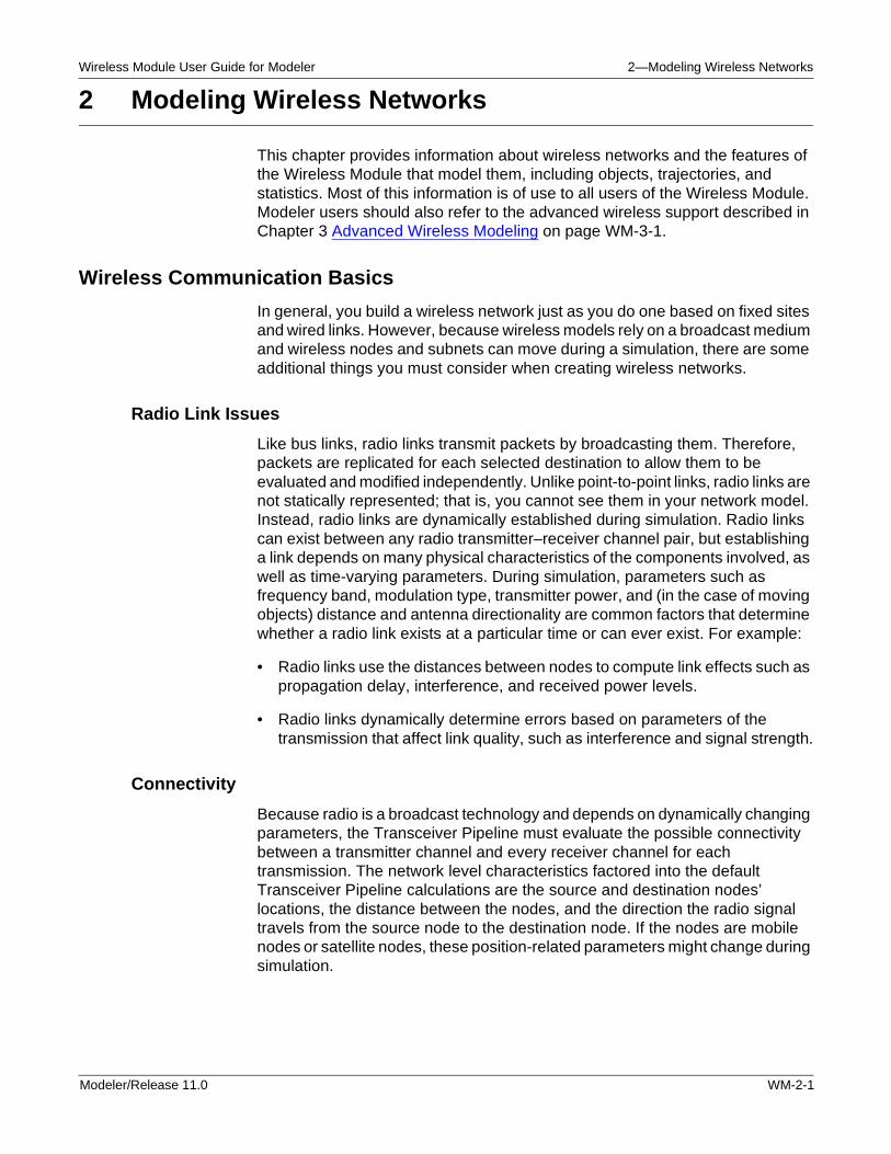
The locations of the nodes are significant factors in a radio link because the default Transceiver Pipeline computes whether the source node has direct line-of-sight to the destination node. Line-of-sight depends on where the nodes are positioned relative to the earth. If the earth’s surface is between the two nodes, then the nodes are said to be occluded and the link computation is discontinued. If the earth or some other object is not between the two nodes, then link closure exists and the link computation continues.

Figure 2-1 Default Model of Occlusion by the Earth’s Surface

The distance between the nodes determines the propagation delay and path loss of the radio signal. The default Transceiver Pipeline computes the propagation delay of the radio signal traveling from the source node to the destination node at the speed of light. The Transceiver Pipeline also models the weakening of the radio signal as it propagates from the source node. It is assumed that the path loss is directly related to the reciprocal of the distance squared.

Antenna Pattern

As a packet is sent from a radio transmitter or received by a radio receiver, the power of the radio signal can be influenced by antennas. In some directions, the signal level is higher and in other directions, lower. Taking this into account, the default Transceiver Pipeline determines the direction in which the radio signal travels from the source node to the destination node. As the signal radiates from the transmitter, the Transceiver Pipeline calculates the signal power out of the antenna in that direction. When the radio signal reaches the destination node, the Transceiver Pipeline also calculates the direction of the signal into the receiver’s antenna (if there is one). The antenna can increase or decrease the received signal based on the incoming direction of the radio signal. As with the transmitter, if a receiver does not have an antenna object attached to it, the signal level is not adjusted.

The earth’s surface does not occlude the source and destination nodes; a radio link is possible.

The earth’s surface occludes the source and destination nodes; no radio link is possible.

WM-2-2 Modeler/Release 11.0


Simulation Efficiency

As indicated in the preceding sections, wireless network simulations involve large number of calculations. For example, OPNET must:

• Test every possible transmitter-receiver combination for each transmitted packet

• Frequently recompute the positions of mobile sites

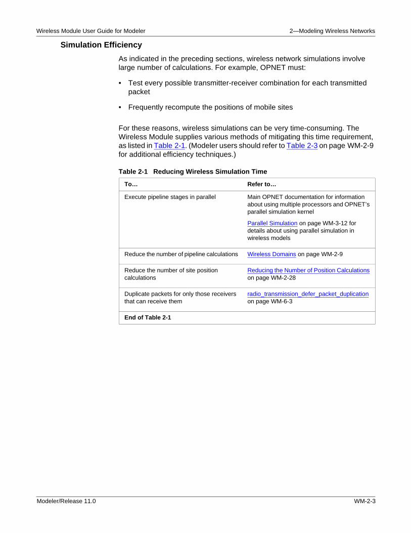
For these reasons, wireless simulations can be very time-consuming. The Wireless Module supplies various methods of mitigating this time requirement, as listed in Table 2-1. (Modeler users should refer to Table 2-3 on page WM-2-9 for additional efficiency techniques.)

Table 2-1 Reducing Wireless Simulation Time

To… Refer to…

Execute pipeline stages in parallel Main OPNET documentation for information about using multiple processors and OPNET’s parallel simulation kernel

Parallel Simulation on page WM-3-12 for details about using parallel simulation in wireless models

Reduce the number of pipeline calculations Wireless Domains on page WM-2-9

Reduce the number of site position calculations

Reducing the Number of Position Calculations on page WM-2-28

Duplicate packets for only those receivers that can receive them

radio_transmission_defer_packet_duplication on page WM-6-3

End of Table 2-1



Wireless Objects

This section provides an overview of the network objects included in the Wireless Module. These objects are radio links and mobile and satellite sites. Detailed information about these objects and their attributes appears in Network Domain on page WM-5-1.

Wireless Subnetworks

The Wireless Module adds two types of subnetworks to the standard OPNET model library: mobile subnets and satellite subnets. Along with fixed subnets, these can contain any combination of fixed and mobile nodes. A subnetwork can also contain other fixed or mobile subnetworks. For example, a satellite subnetwork representing a space station could contain fixed subnets (representing LANs), mobile subnets (representing individual astronauts carrying various pieces of communications equipment), fixed nodes (representing radio transceivers), and mobile nodes (representing portable computers).

Mobile Subnetworks

A mobile subnetwork can change positions during a simulation via one of three mechanisms: pre-defined trajectory segments, vector trajectory, or direct changes to the subnetwork’s position attributes. If trajectory segments are specified, the subnetwork’s position is automatically updated at appropriate times to follow that trajectory during simulation. Refer to Trajectories on page WM-2-12 for more information on trajectories.

Mobile subnetworks are typically used to contain networks whose overall position varies with time, such as a submarine, a ship, or an airplane. Because mobile subnetworks move relative to the earth, objects within them cannot be connected to other objects outside the network with point-to-point or bus links.

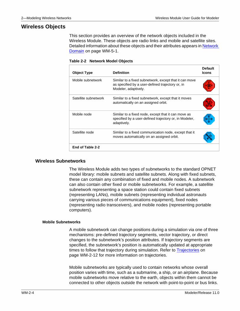
Table 2-2 Network Model Objects

Object Type DefinitionDefault Icons

Mobile subnetwork Similar to a fixed subnetwork, except that it can move as specified by a user-defined trajectory or, in Modeler, adaptively.

Satellite subnetwork Similar to a fixed subnetwork, except that it moves automatically on an assigned orbit.

Mobile node Similar to a fixed node, except that it can move as specified by a user-defined trajectory or, in Modeler, adaptively.

Satellite node Similar to a fixed communication node, except that it moves automatically on an assigned orbit.

End of Table 2-2



Satellite Subnetworks

A satellite subnetwork can change position during a simulation via an assigned orbit, which specifies its orbital path through time. The satellite subnetwork’s position is automatically updated at appropriate times during simulation to follow that orbit (refer to Orbits on page WM-2-19 for more information). Because satellite subnetworks move relative to the earth, objects within them cannot be connected to other objects outside the network with point-to-point or bus links.

Wireless Communication Nodes

The Wireless Module adds two types of communication nodes to OPNET’s standard model library: mobile nodes and satellite nodes. Both types of nodes are similar to fixed communication nodes, except that they can change position during simulation. Mobile nodes can follow a pre-defined trajectory or move based on decisions made by processes within the node, whereas satellite nodes automatically follow an assigned orbit as a function of time. Both types of nodes are described in this section.

Mobile Nodes

Mobile nodes model network elements whose positions vary with time, such as automobiles, aircraft, and ships. They are normally placed within a subnetwork other than the top subnet, because a subnetwork object has the capability to define a region that is dimensioned in units that are appropriate for the range of the mobile nodes. For example, a subnetwork object can be used to define the area of a building, where hand-held communication units are represented by mobile nodes, or the subnetwork can be used to define the area of a city, where automobiles with cellular telephones are represented by mobile nodes.

A mobile communication node can change positions during a simulation via one of three mechanisms: either by trajectory segments, by a vector trajectory, or (using Modeler) by direct changes to the node’s position attributes. If a trajectory is specified, the node’s position is automatically updated at appropriate times to follow that trajectory during simulation, as described in Trajectories on page WM-2-12. Because mobile nodes move relative to the earth, they cannot be connected to point-to-point and bus links.

Satellite Nodes

Satellite communication nodes model satellite objects, whose positions vary with time. A satellite node moves according to an assigned orbit that specifies its path around the earth, as described in Orbits on page WM-2-19. The satellite node’s position is automatically updated at appropriate times during simulation to follow that orbit. If a subnetwork contains a satellite node with an assigned orbit, the parent subnetwork’s location and size do not affect the satellite’s orbital path. This is in contrast to fixed and mobile nodes, whose positions are often defined relative to their parent subnetworks. Because satellites move around the earth, satellite nodes communicate via radio links; they cannot be connected to point-to-point or bus links.



Wireless Communication Links

The Wireless Module adds radio links to OPNET. Radio links exist as a function of dynamic conditions and so are not represented by objects. Instead they result from a dynamic evaluation by the Simulation Kernel. Radio links potentially allow all nodes in a model to communicate with each other, based on a dynamic evaluation.

Radio Links

A radio link might exist between any radio transmitter-receiver channel pair and is dynamically established during simulation. The possibility of a radio link between a transmitter channel and a receiver channel can be dependent on many physical characteristics of the components involved, as well as time-varying parameters. In OPNET simulations, parameters such as frequency band, modulation type, transmitter power, distance, and antenna directionality are commonly factored into the determination of whether a radio link exists or not at a particular time. Therefore, a radio link is not statically represented by an object, as are point-to-point and bus links.

Correspondingly, radio transmitter and receiver objects have a greater role in determining the behavior of a radio link. Unlike point-to-point and bus link objects which have attributes to specify the pipeline stages, a radio link is not an object and cannot provide those values. Therefore, the radio transmitter and receiver objects’ attributes identify the appropriate pipeline stage values that make up the transceiver pipeline, which performs the calculations required to determine when and if a packet is successfully received. For a full description of the Radio Transceiver Pipeline, refer to Chapter 10 Radio Transceiver Pipeline on page WM-10-1. The remainder of this section explains how the network-level objects (nodes and subnets) affect the default radio transceiver pipeline.

Because radio is a broadcast technology and depends on dynamically changing parameters, the transceiver pipeline must evaluate the possible connectivity between a transmitter channel and every receiver channel for each transmission. The network level characteristics factored into the default transceiver pipeline calculations are the source and destination sites’ locations, the distance between the sites, and the direction the radio signal travels from the source site to the destination site. If the sites are mobile or satellite sites, then these position-related parameters can change during simulation.

The locations of the sites are significant factors in a radio link, because the default transceiver pipeline computes whether the source site has direct line of sight to the destination node. Line of sight depends on where the sites are positioned relative to the earth. If the earth’s surface is between the two sites, then the sites are said to be occluded and the computation of the radio link is discontinued. If the earth is not between the two sites, then link closure is said to exist and the computation of the link continues. If you are using terrain modeling, link closure can be affected by terrain features such as hills, in addition to the earth’s curvature.



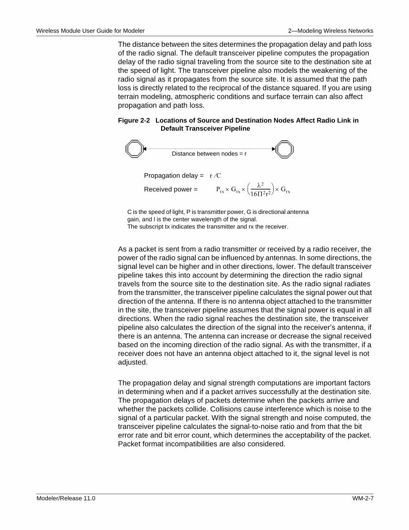
The distance between the sites determines the propagation delay and path loss of the radio signal. The default transceiver pipeline computes the propagation delay of the radio signal traveling from the source site to the destination site at the speed of light. The transceiver pipeline also models the weakening of the radio signal as it propagates from the source site. It is assumed that the path loss is directly related to the reciprocal of the distance squared. If you are using terrain modeling, atmospheric conditions and surface terrain can also affect propagation and path loss.

Figure 2-2 Locations of Source and Destination Nodes Affect Radio Link in Default Transceiver Pipeline

As a packet is sent from a radio transmitter or received by a radio receiver, the power of the radio signal can be influenced by antennas. In some directions, the signal level can be higher and in other directions, lower. The default transceiver pipeline takes this into account by determining the direction the radio signal travels from the source site to the destination site. As the radio signal radiates from the transmitter, the transceiver pipeline calculates the signal power out that direction of the antenna. If there is no antenna object attached to the transmitter in the site, the transceiver pipeline assumes that the signal power is equal in all directions. When the radio signal reaches the destination site, the transceiver pipeline also calculates the direction of the signal into the receiver’s antenna, if there is an antenna. The antenna can increase or decrease the signal received based on the incoming direction of the radio signal. As with the transmitter, if a receiver does not have an antenna object attached to it, the signal level is not adjusted.

The propagation delay and signal strength computations are important factors in determining when and if a packet arrives successfully at the destination site. The propagation delays of packets determine when the packets arrive and whether the packets collide. Collisions cause interference which is noise to the signal of a particular packet. With the signal strength and noise computed, the transceiver pipeline calculates the signal-to-noise ratio and from that the bit error rate and bit error count, which determines the acceptability of the packet. Packet format incompatibilities are also considered.

Propagation delay =

Received power = Ptx Gtxλ2

16Π2r2------------------ Grx×××

r C⁄

C is the speed of light, P is transmitter power, G is directional antenna gain, and l is the center wavelength of the signal. The subscript tx indicates the transmitter and rx the receiver.

Distance between nodes = r



Radio Link Details

Note—This section provides additional information about radio links for Modeler users.

From the perspective of the modules within a node, radio links are used in the same manner as point-to-point and bus links. In other words, if a module wishes to send a packet via a radio link, it must send the packet to one of the input streams of a radio transmitter. The radio transmitter is then responsible for sending the packet to radio receivers in remote nodes. These radio receivers in turn issue correctly received packets on appropriate output streams.

Like a bus or point-to-point transmitter, a radio transmitter maintains a channel object for each of its input streams and each channel contains a queue where submitted packets wait for previous packets to complete transmission. However, whereas bus and point-to-point transmitter channels have primarily a logical significance, radio transmitter channels also have a physical significance that is described by an additional set of attributes. These additional attributes characterize the radio channel in terms of the frequency band it occupies, the power applied to transmissions, the data rate of transmission, and an optional code used to identify a spread spectrum sequence.

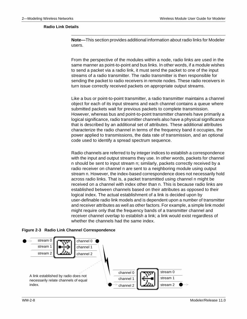
Radio channels are referred to by integer indices to establish a correspondence with the input and output streams they use. In other words, packets for channel n should be sent to input stream n; similarly, packets correctly received by a radio receiver on channel n are sent to a neighboring module using output stream n. However, the index-based correspondence does not necessarily hold across radio links. That is, a packet transmitted using channel n might be received on a channel with index other than n. This is because radio links are established between channels based on their attributes as opposed to their logical index. The actual establishment of a link is decided upon by user-definable radio link models and is dependent upon a number of transmitter and receiver attributes as well as other factors. For example, a simple link model might require only that the frequency bands of a transmitter channel and receiver channel overlap to establish a link; a link would exist regardless of whether the channels had the same index.

Figure 2-3 Radio Link Channel Correspondence

A link established by radio does not necessarily relate channels of equal index.

channel 0

channel 1

channel 2

channel 0

channel 1

channel 2

stream 0

stream 1

stream 2

stream 0

stream 1

stream 2



Like bus transmitters, radio transmitters transmit packets by broadcasting them. Therefore, packets are replicated for each selected destination to allow them to be evaluated and modified independently. Note that, unlike bus links, replication is on a per-channel basis at the destination, because a single packet can affect multiple channels within a radio receiver. Again, this is due to the fact that channels are compared on the basis of their physical characteristics, rather than their logical index values.

The eligible receivers of each radio transmitter are not necessarily known in advance, as in the usual case of a bus configuration. Instead, the existence and quality of each link is generally computed on a dynamic basis to reflect potentially changing conditions in the network. Important events, such as position changes and interference, can have a significant impact on the ability of a transmitter channel and a receiver channel to communicate, and these events might occur at any time. The detailed behavior and mechanics of radio transmissions are specified in a series of low-level radio models, referred to as pipeline stages. The theory and operation of radio pipeline stages are described in detail in Chapter 10 Radio Transceiver Pipeline on page WM-10-1.

In addition to the methods given in Table 2-1 on page WM-2-3, Modeler users can apply the following methods to reduce the amount of time spent on pipeline calculations:

Wireless Domains

As described in Wireless Communication Links on page WM-2-6, the Simulation Kernel must do many calculations for each packet sent across a radio link. These calculations are done for each channel that might be able to receive the transmitted packet. Wireless domains provide a way to reduce the number of calculations that must be done, thus reducing the time needed for a wireless simulation to run (at the cost of increased memory use).

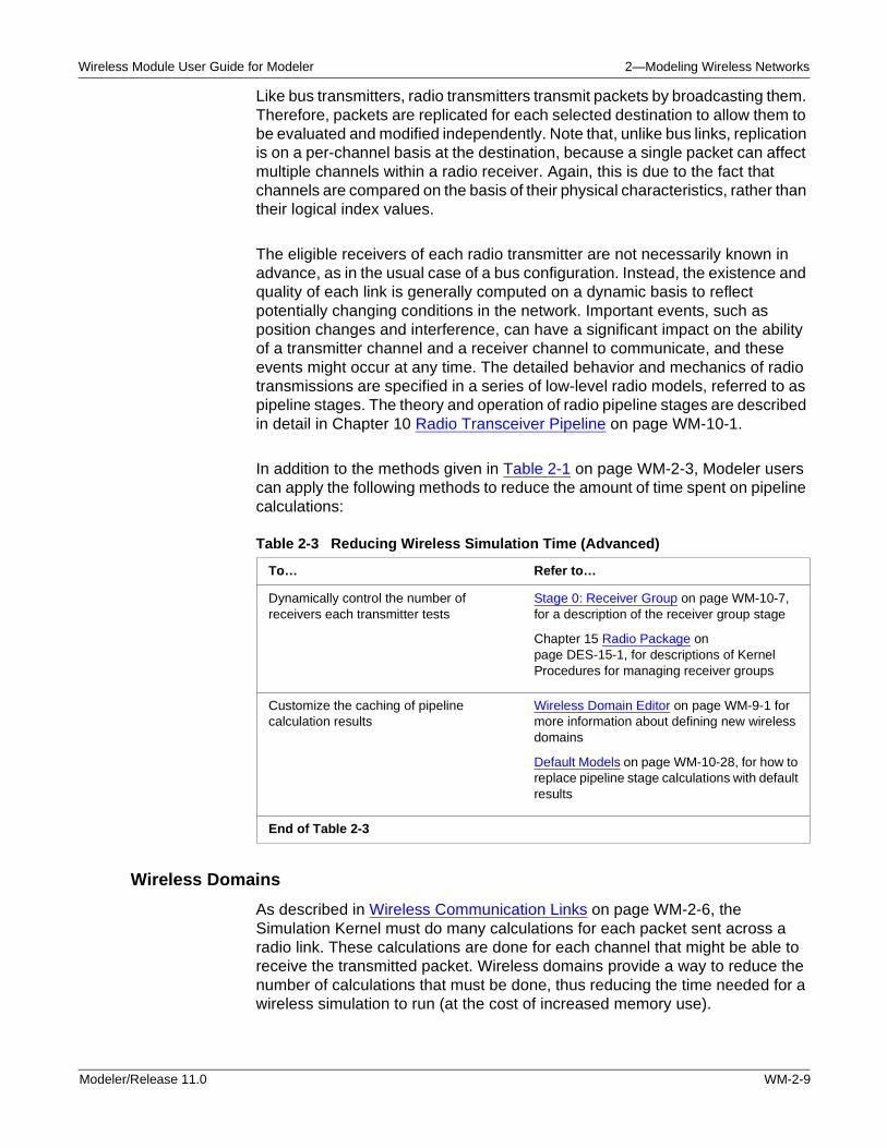
Table 2-3 Reducing Wireless Simulation Time (Advanced)

To… Refer to…

Dynamically control the number of receivers each transmitter tests

Stage 0: Receiver Group on page WM-10-7, for a description of the receiver group stage

Chapter 15 Radio Package on page DES-15-1, for descriptions of Kernel Procedures for managing receiver groups

Customize the caching of pipeline calculation results

Wireless Domain Editor on page WM-9-1 for more information about defining new wireless domains

Default Models on page WM-10-28, for how to replace pipeline stage calculations with default results

End of Table 2-3



A wireless domain defines a rectangular area that is subdivided into a logical grid of clusters. Each cluster represents an area in which any contained nodes are assumed to have the same characteristics (such as path loss) with respect to nodes in other clusters of the domain. The wireless domain saves selected results of the radio pipeline calculations and reuses them for future communications between the same clusters. The results that can be saved for reuse are:

• Channel match

• Closure

• Propagation delay

• Path loss

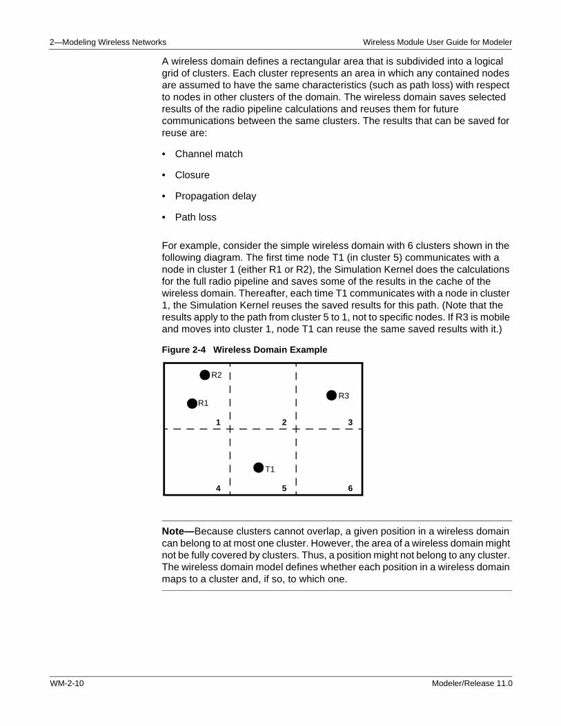
For example, consider the simple wireless domain with 6 clusters shown in the following diagram. The first time node T1 (in cluster 5) communicates with a node in cluster 1 (either R1 or R2), the Simulation Kernel does the calculations for the full radio pipeline and saves some of the results in the cache of the wireless domain. Thereafter, each time T1 communicates with a node in cluster 1, the Simulation Kernel reuses the saved results for this path. (Note that the results apply to the path from cluster 5 to 1, not to specific nodes. If R3 is mobile and moves into cluster 1, node T1 can reuse the same saved results with it.)

Figure 2-4 Wireless Domain Example

Note—Because clusters cannot overlap, a given position in a wireless domain can belong to at most one cluster. However, the area of a wireless domain might not be fully covered by clusters. Thus, a position might not belong to any cluster. The wireless domain model defines whether each position in a wireless domain maps to a cluster and, if so, to which one.

1 2 3

4 5 6

T1

R2

R1R3



Although the technique of reusing certain pipeline stage calculations introduces some approximation into a simulation, it is small for well-chosen cluster sizes and does not affect simulation results appreciably.

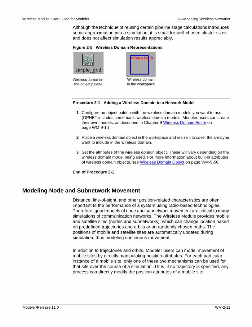
Figure 2-5 Wireless Domain Representations

Procedure 2-1 Adding a Wireless Domain to a Network Model

1 Configure an object palette with the wireless domain models you want to use. (OPNET includes some basic wireless domain models. Modeler users can create their own models, as described in Chapter 9 Wireless Domain Editor on page WM-9-1.)

2 Place a wireless domain object in the workspace and resize it to cover the area you want to include in the wireless domain.

3 Set the attributes of the wireless domain object. These will vary depending on the wireless domain model being used. For more information about built-in attributes of wireless domain objects, see Wireless Domain Object on page WM-5-50.

End of Procedure 2-1

Modeling Node and Subnetwork Movement

Distance, line-of-sight, and other position-related characteristics are often important to the performance of a system using radio-based technologies. Therefore, good models of node and subnetwork movement are critical to many simulations of communication networks. The Wireless Module provides mobile and satellite sites (nodes and subnetworks), which can change location based on predefined trajectories and orbits or on randomly chosen paths. The positions of mobile and satellite sites are automatically updated during simulation, thus modeling continuous movement.

In addition to trajectories and orbits, Modeler users can model movement of mobile sites by directly manipulating position attributes. For each particular instance of a mobile site, only one of these two mechanisms can be used for that site over the course of a simulation. Thus, if no trajectory is specified, any process can directly modify the position attributes of a mobile site.

Wireless domain in the object palette

Wireless domain in the workspace



Trajectories

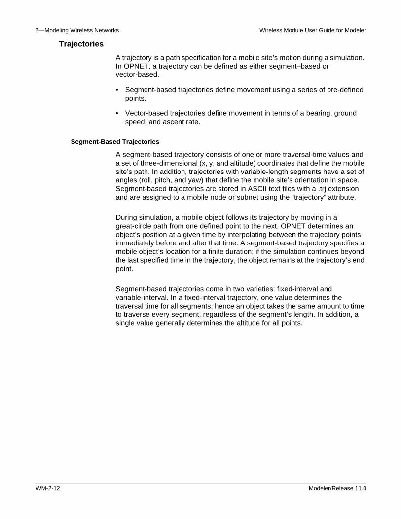
A trajectory is a path specification for a mobile site’s motion during a simulation. In OPNET, a trajectory can be defined as either segment–based or vector-based.

• Segment-based trajectories define movement using a series of pre-defined points.

• Vector-based trajectories define movement in terms of a bearing, ground speed, and ascent rate.

Segment-Based Trajectories

A segment-based trajectory consists of one or more traversal-time values and a set of three-dimensional (x, y, and altitude) coordinates that define the mobile site’s path. In addition, trajectories with variable-length segments have a set of angles (roll, pitch, and yaw) that define the mobile site’s orientation in space. Segment-based trajectories are stored in ASCII text files with a .trj extension and are assigned to a mobile node or subnet using the “trajectory” attribute.

During simulation, a mobile object follows its trajectory by moving in a great-circle path from one defined point to the next. OPNET determines an object’s position at a given time by interpolating between the trajectory points immediately before and after that time. A segment-based trajectory specifies a mobile object’s location for a finite duration; if the simulation continues beyond the last specified time in the trajectory, the object remains at the trajectory’s end point.

Segment-based trajectories come in two varieties: fixed-interval and variable-interval. In a fixed-interval trajectory, one value determines the traversal time for all segments; hence an object takes the same amount to time to traverse every segment, regardless of the segment’s length. In addition, a single value generally determines the altitude for all points.



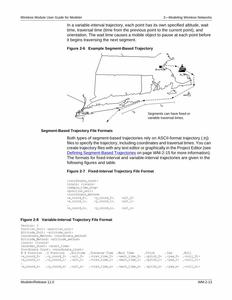
In a variable-interval trajectory, each point has its own specified altitude, wait time, traversal time (time from the previous point to the current point), and orientation. The wait time causes a mobile object to pause at each point before it begins traversing the next segment.

Figure 2-6 Example Segment-Based Trajectory

Segment-Based Trajectory File Formats

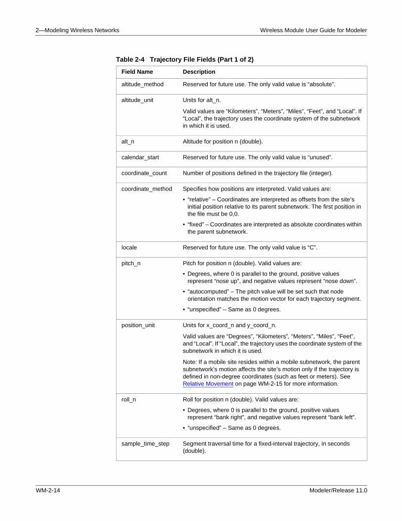
Both types of segment-based trajectories rely on ASCII-format trajectory (.trj) files to specify the trajectory, including coordinates and traversal times. You can create trajectory files with any text editor or graphically in the Project Editor (see Defining Segment-Based Trajectories on page WM-2-15 for more information). The formats for fixed-interval and variable-interval trajectories are given in the following figures and table.

Figure 2-7 Fixed-Interval Trajectory File Format

<coordinate_count>locale: <locale><sample_time_step><position_unit><coordinate_method><x_coord_0>, <y_coord_0>, <alt_0><x_coord_1>, <y_coord_1>, <alt_1>…<x_coord_n>, <y_coord_n>, <alt_n>

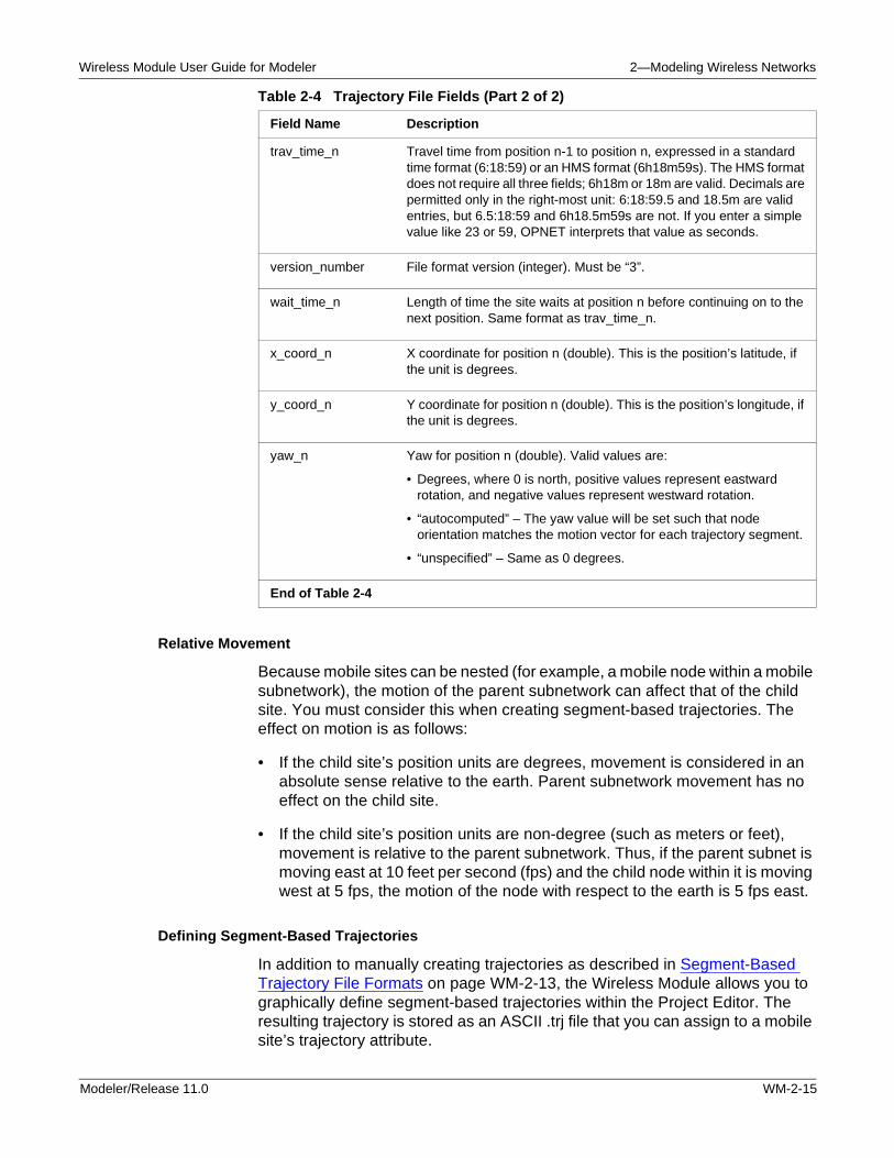
Figure 2-8 Variable-Interval Trajectory File Format

Segments can have fixed or variable traversal times.

τ5

τ6

Version: 3Position_Unit: <position_unit>Altitude_Unit: <altitude_unit>Coordinate_Method: <coordinate_method>Altitude_Method: <altitude_method>locale: <locale>Calendar_Start: <start_time>Coordinate Count: <coordinate_count># X Position ,Y Position ,Altitude ,Traverse Time ,Wait Time ,Pitch ,Yaw ,Roll<x_coord_0> ,<y_coord_0> ,<alt_0> ,<trav_time_0> ,<wait_time_0> ,<pitch_0> ,<yaw_0> ,<roll_0)><x_coord_1> ,<y_coord_1> ,<alt_1> ,<trav_time_1> ,<wait_time_1> ,<pitch_1> ,<yaw_1> ,<roll_1)>…<x_coord_n> ,<y_coord_n> ,<alt_n> ,<trav_time_n> ,<wait_time_n> ,<pitch_n> ,<yaw_n> ,<roll_n)>



Table 2-4 Trajectory File Fields (Part 1 of 2)

Field Name Description

altitude_method Reserved for future use. The only valid value is “absolute”.

altitude_unit Units for alt_n.

Valid values are “Kilometers”, “Meters”, “Miles”, “Feet”, and “Local”. If “Local”, the trajectory uses the coordinate system of the subnetwork in which it is used.

alt_n Altitude for position n (double).

calendar_start Reserved for future use. The only valid value is “unused”.

coordinate_count Number of positions defined in the trajectory file (integer).

coordinate_method Specifies how positions are interpreted. Valid values are:

• “relative” – Coordinates are interpreted as offsets from the site’s initial position relative to its parent subnetwork. The first position in the file must be 0,0.

• “fixed” – Coordinates are interpreted as absolute coordinates within the parent subnetwork.

locale Reserved for future use. The only valid value is “C”.

pitch_n Pitch for position n (double). Valid values are:

• Degrees, where 0 is parallel to the ground, positive values represent “nose up”, and negative values represent “nose down”.

• “autocomputed” – The pitch value will be set such that node orientation matches the motion vector for each trajectory segment.

• “unspecified” – Same as 0 degrees.

position_unit Units for x_coord_n and y_coord_n.

Valid values are “Degrees”, “Kilometers”, “Meters”, “Miles”, “Feet”, and “Local”. If “Local”, the trajectory uses the coordinate system of the subnetwork in which it is used.

Note: If a mobile site resides within a mobile subnetwork, the parent subnetwork’s motion affects the site’s motion only if the trajectory is defined in non-degree coordinates (such as feet or meters). See Relative Movement on page WM-2-15 for more information.

roll_n Roll for position n (double). Valid values are:

• Degrees, where 0 is parallel to the ground, positive values represent “bank right”, and negative values represent “bank left”.


sample_time_step Segment traversal time for a fixed-interval trajectory, in seconds (double).



Relative Movement

Because mobile sites can be nested (for example, a mobile node within a mobile subnetwork), the motion of the parent subnetwork can affect that of the child site. You must consider this when creating segment-based trajectories. The effect on motion is as follows:

• If the child site’s position units are degrees, movement is considered in an absolute sense relative to the earth. Parent subnetwork movement has no effect on the child site.

• If the child site’s position units are non-degree (such as meters or feet), movement is relative to the parent subnetwork. Thus, if the parent subnet is moving east at 10 feet per second (fps) and the child node within it is moving west at 5 fps, the motion of the node with respect to the earth is 5 fps east.

Defining Segment-Based Trajectories

In addition to manually creating trajectories as described in Segment-Based Trajectory File Formats on page WM-2-13, the Wireless Module allows you to graphically define segment-based trajectories within the Project Editor. The resulting trajectory is stored as an ASCII .trj file that you can assign to a mobile site’s trajectory attribute.

trav_time_n Travel time from position n-1 to position n, expressed in a standard time format (6:18:59) or an HMS format (6h18m59s). The HMS format does not require all three fields; 6h18m or 18m are valid. Decimals are permitted only in the right-most unit: 6:18:59.5 and 18.5m are valid entries, but 6.5:18:59 and 6h18.5m59s are not. If you enter a simple value like 23 or 59, OPNET interprets that value as seconds.

version_number File format version (integer). Must be “3”.

wait_time_n Length of time the site waits at position n before continuing on to the next position. Same format as trav_time_n.

x_coord_n X coordinate for position n (double). This is the position’s latitude, if the unit is degrees.

y_coord_n Y coordinate for position n (double). This is the position’s longitude, if the unit is degrees.

yaw_n Yaw for position n (double). Valid values are:

• Degrees, where 0 is north, positive values represent eastward rotation, and negative values represent westward rotation.

• “autocomputed” – The yaw value will be set such that node orientation matches the motion vector for each trajectory segment.


End of Table 2-4

Table 2-4 Trajectory File Fields (Part 2 of 2)

Field Name Description



The procedure for defining a trajectory varies slightly depending on whether the trajectory uses fixed intervals or variable intervals. The following procedure describes these variations where applicable.

Procedure 2-2 Defining a Segment-Based Trajectory

1 In the Project Editor, choose Topology > Define Trajectory…

➥ The Define Trajectory dialog box appears.

2 Enter a name for the trajectory.

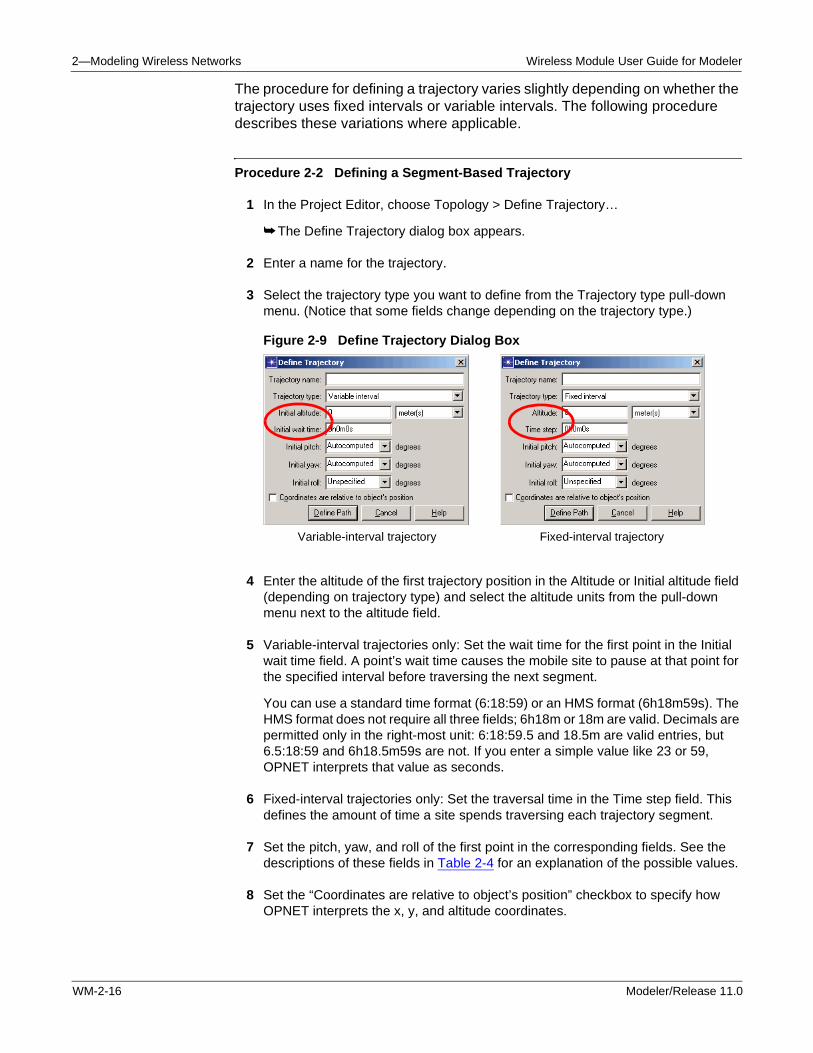
3 Select the trajectory type you want to define from the Trajectory type pull-down menu. (Notice that some fields change depending on the trajectory type.)

Figure 2-9 Define Trajectory Dialog Box

4 Enter the altitude of the first trajectory position in the Altitude or Initial altitude field (depending on trajectory type) and select the altitude units from the pull-down menu next to the altitude field.

5 Variable-interval trajectories only: Set the wait time for the first point in the Initial wait time field. A point’s wait time causes the mobile site to pause at that point for the specified interval before traversing the next segment.

You can use a standard time format (6:18:59) or an HMS format (6h18m59s). The HMS format does not require all three fields; 6h18m or 18m are valid. Decimals are permitted only in the right-most unit: 6:18:59.5 and 18.5m are valid entries, but 6.5:18:59 and 6h18.5m59s are not. If you enter a simple value like 23 or 59, OPNET interprets that value as seconds.

6 Fixed-interval trajectories only: Set the traversal time in the Time step field. This defines the amount of time a site spends traversing each trajectory segment.

7 Set the pitch, yaw, and roll of the first point in the corresponding fields. See the descriptions of these fields in Table 2-4 for an explanation of the possible values.

8 Set the “Coordinates are relative to object’s position” checkbox to specify how OPNET interprets the x, y, and altitude coordinates.

Variable-interval trajectory Fixed-interval trajectory



If this checkbox is selected, the x and y coordinates are relative offsets from the mobile site’s initial position with respect to its parent subnet (as specified by the mobile site’s x position, y position, and altitude attributes).

If this checkbox is unselected, the coordinates are considered absolute values. The trajectory’s position coordinates replace the site’s x position, y position, and altitude attribute values.

9 Click the Define Path button.

➥ A Trajectory Status dialog box opens and a thin diagonal line appears above the cursor in the Project Editor workspace.

10 Define the trajectory points, as follows.

• Fixed-interval trajectory—Left-click at the desired location of each point in the trajectory. When you have defined all the points, right-click in the workspace and choose “Complete trajectory definition” from the pop-up menu.

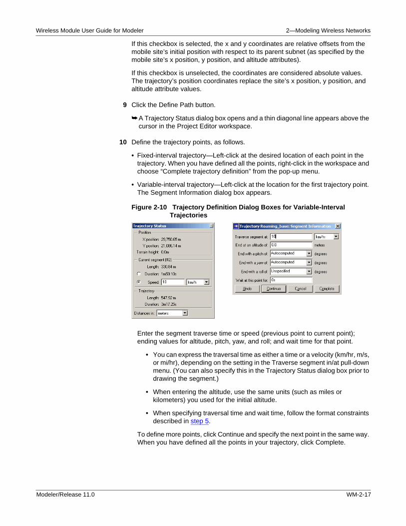
• Variable-interval trajectory—Left-click at the location for the first trajectory point. The Segment Information dialog box appears.

Figure 2-10 Trajectory Definition Dialog Boxes for Variable-Interval Trajectories

Enter the segment traverse time or speed (previous point to current point); ending values for altitude, pitch, yaw, and roll; and wait time for that point.

• You can express the traversal time as either a time or a velocity (km/hr, m/s, or mi/hr), depending on the setting in the Traverse segment in/at pull-down menu. (You can also specify this in the Trajectory Status dialog box prior to drawing the segment.)

• When entering the altitude, use the same units (such as miles or kilometers) you used for the initial altitude.

• When specifying traversal time and wait time, follow the format constraints described in step 5.

To define more points, click Continue and specify the next point in the same way. When you have defined all the points in your trajectory, click Complete.



11 When you complete a trajectory definition, the trajectory is saved as an ASCII file with a .trj suffix in your primary models directory.


Vector-Based Trajectories

A vector-based trajectory consists of a direction and a velocity that can be changed at run time. You specify that a site will use a vector-based trajectory by setting the site’s trajectory attribute to VECTOR.

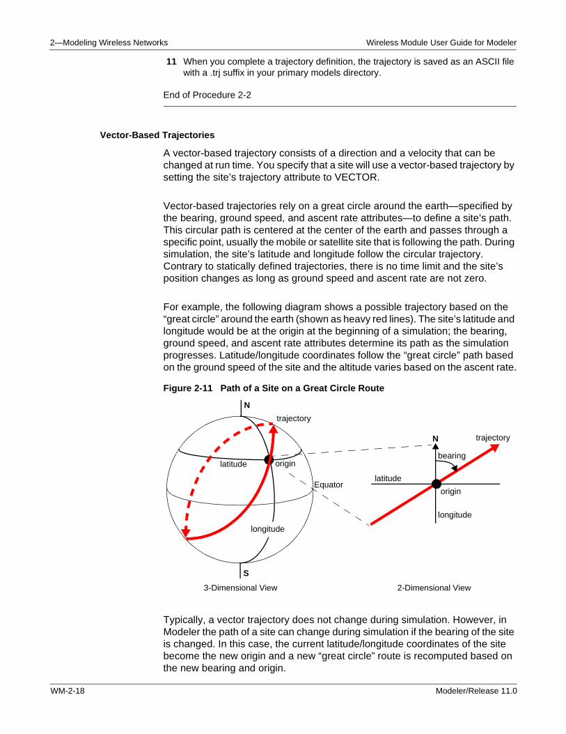
Vector-based trajectories rely on a great circle around the earth—specified by the bearing, ground speed, and ascent rate attributes—to define a site’s path. This circular path is centered at the center of the earth and passes through a specific point, usually the mobile or satellite site that is following the path. During simulation, the site’s latitude and longitude follow the circular trajectory. Contrary to statically defined trajectories, there is no time limit and the site’s position changes as long as ground speed and ascent rate are not zero.

For example, the following diagram shows a possible trajectory based on the “great circle” around the earth (shown as heavy red lines). The site’s latitude and longitude would be at the origin at the beginning of a simulation; the bearing, ground speed, and ascent rate attributes determine its path as the simulation progresses. Latitude/longitude coordinates follow the “great circle” path based on the ground speed of the site and the altitude varies based on the ascent rate.

Figure 2-11 Path of a Site on a Great Circle Route

Typically, a vector trajectory does not change during simulation. However, in Modeler the path of a site can change during simulation if the bearing of the site is changed. In this case, the current latitude/longitude coordinates of the site become the new origin and a new “great circle” route is recomputed based on the new bearing and origin.

3-Dimensional View 2-Dimensional View

trajectory

latitude

longitude

origin

Equatorlatitude

longitude

trajectory

origin

bearing

N

N

S



Orbits

Satellite sites use an orbit to specify their location during a simulation. An orbit is the path around the earth along which the satellite site moves during simulation. If a subnetwork contains a satellite site with an assigned orbit, the parent subnetwork’s location and size do not affect the satellite’s orbital path. This is in contrast to fixed and mobile sites, whose positions are often defined relative to their parent subnetworks.

An orbit is defined by an orbit file, which holds data specifying the times and locations that the satellite site will pass through as the simulation progresses. You create orbit files using the Satellite Tool Kit program from Analytical Graphics, and then import the files into OPNET. (See Satellite Took Kit on page WM-2-20 for more information on the Satellite Tool Kit.) The Satellite Tool Kit uses six orbital elements to compute the orbit at a set of discrete points evenly sampled in time. In addition, Modeler users can create orbits via EMA (see External Model Access on page MFA-1-1 in the Model File Access API Reference Manual).

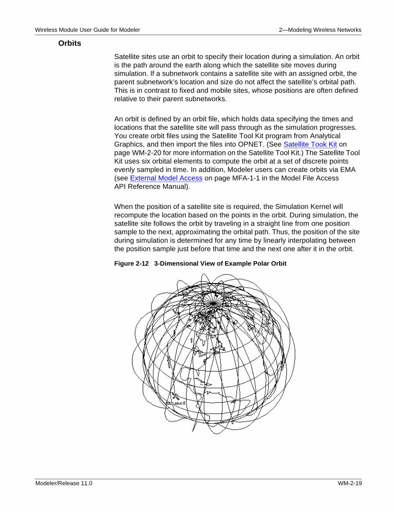
When the position of a satellite site is required, the Simulation Kernel will recompute the location based on the points in the orbit. During simulation, the satellite site follows the orbit by traveling in a straight line from one position sample to the next, approximating the orbital path. Thus, the position of the site during simulation is determined for any time by linearly interpolating between the position sample just before that time and the next one after it in the orbit.

Figure 2-12 3-Dimensional View of Example Polar Orbit



While satellite sites with orbits are useful for modeling satellites that move relative to the earth’s surface, some satellites’ motion can be modeled without an orbit. Because a geostationary satellite maintains a relatively fixed position over one point on the earth’s surface, a satellite site without a specified orbit can be an appropriate model. If the orbit attribute of a satellite site is set to NONE, then the initial values of the position attributes are used, as if the site were fixed to that location over the earth. This provides an increase in simulation efficiency, because the site’s position does not need to be recomputed each time that it is required. However, if the slight perturbations of a satellite’s position in geostationary orbit are important, then a geostationary orbit should be specified.

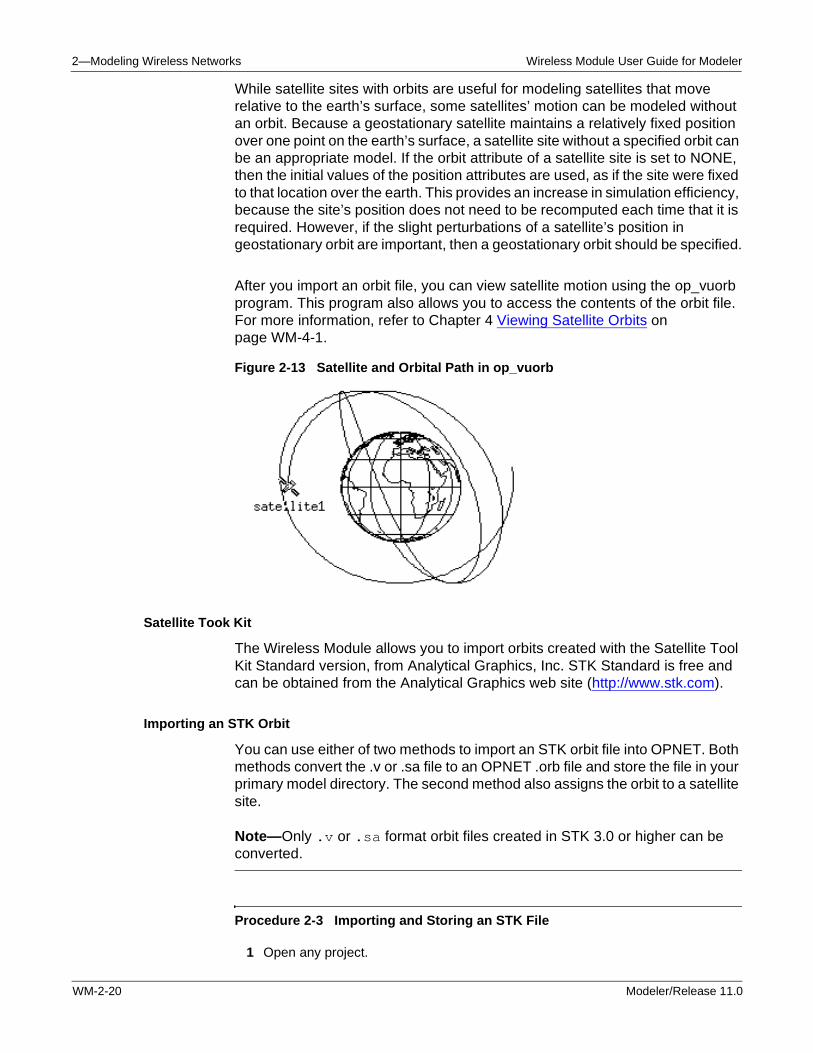
After you import an orbit file, you can view satellite motion using the op_vuorb program. This program also allows you to access the contents of the orbit file. For more information, refer to Chapter 4 Viewing Satellite Orbits on page WM-4-1.

Figure 2-13 Satellite and Orbital Path in op_vuorb

Satellite Took Kit

The Wireless Module allows you to import orbits created with the Satellite Tool Kit Standard version, from Analytical Graphics, Inc. STK Standard is free and can be obtained from the Analytical Graphics web site (http://www.stk.com).

Importing an STK Orbit

You can use either of two methods to import an STK orbit file into OPNET. Both methods convert the .v or .sa file to an OPNET .orb file and store the file in your primary model directory. The second method also assigns the orbit to a satellite site.

Note—Only .v or .sa format orbit files created in STK 3.0 or higher can be converted.

Procedure 2-3 Importing and Storing an STK File

1 Open any project.


http://www.stk.com


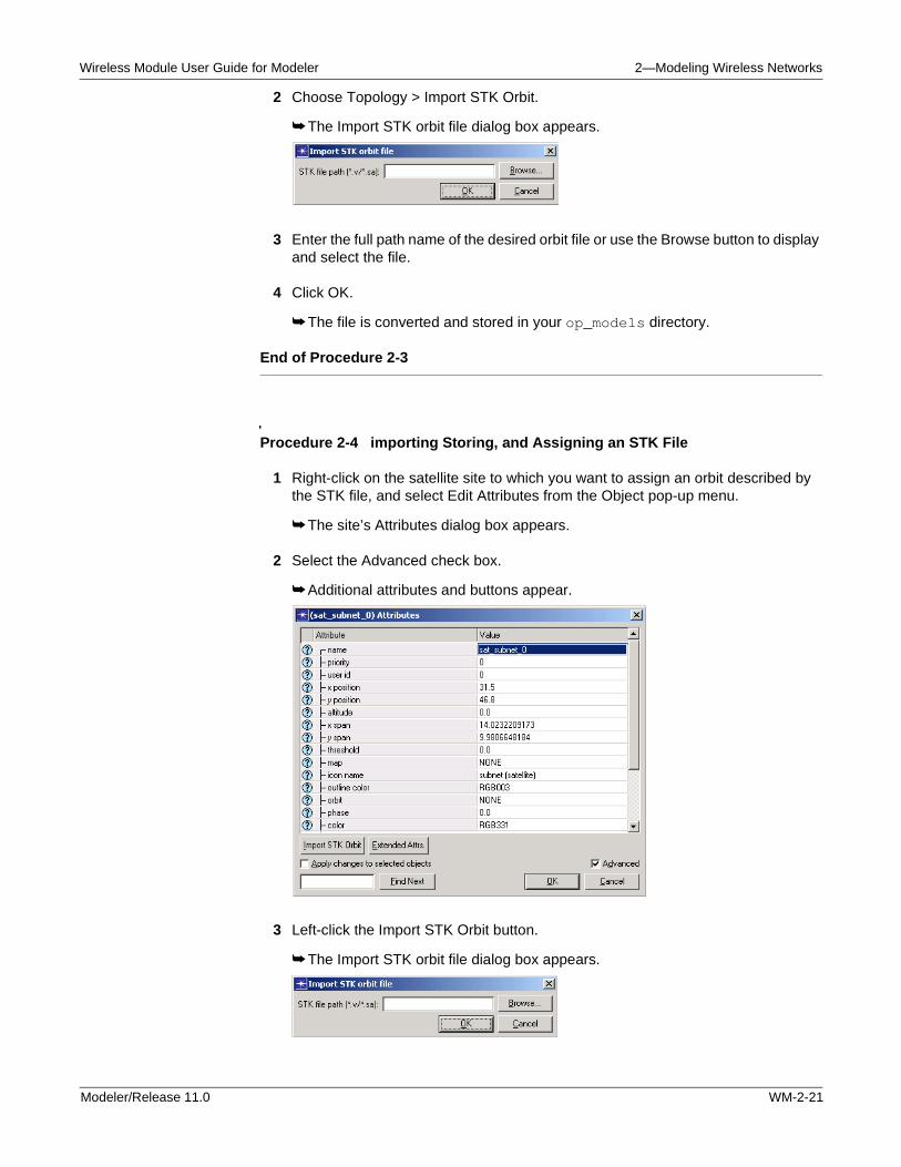
2 Choose Topology > Import STK Orbit.

➥ The Import STK orbit file dialog box appears.

3 Enter the full path name of the desired orbit file or use the Browse button to display and select the file.

4 Click OK.

➥ The file is converted and stored in your op_models directory.


Procedure 2-4 importing Storing, and Assigning an STK File

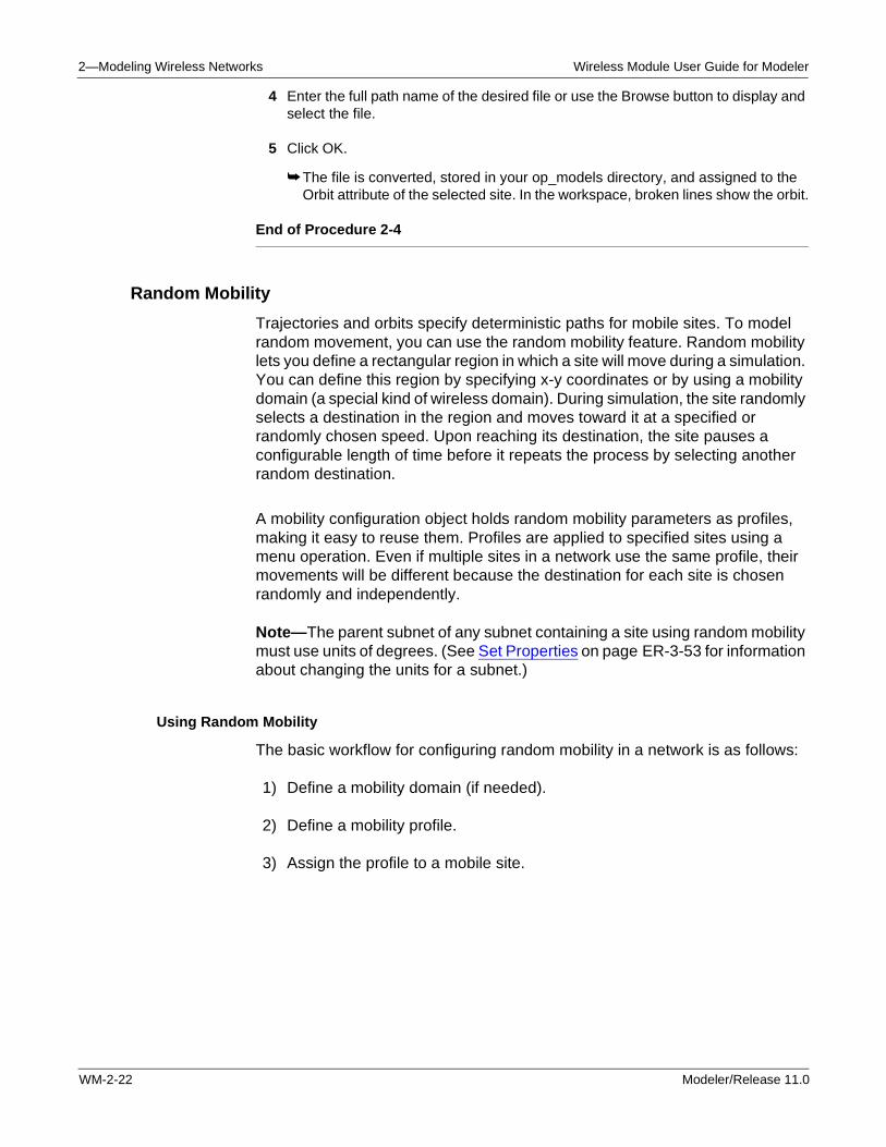
1 Right-click on the satellite site to which you want to assign an orbit described by the STK file, and select Edit Attributes from the Object pop-up menu.

➥ The site’s Attributes dialog box appears.

2 Select the Advanced check box.

➥ Additional attributes and buttons appear.

3 Left-click the Import STK Orbit button.

➥ The Import STK orbit file dialog box appears.



4 Enter the full path name of the desired file or use the Browse button to display and select the file.

5 Click OK.

➥ The file is converted, stored in your op_models directory, and assigned to the Orbit attribute of the selected site. In the workspace, broken lines show the orbit.


Random Mobility

Trajectories and orbits specify deterministic paths for mobile sites. To model random movement, you can use the random mobility feature. Random mobility lets you define a rectangular region in which a site will move during a simulation. You can define this region by specifying x-y coordinates or by using a mobility domain (a special kind of wireless domain). During simulation, the site randomly selects a destination in the region and moves toward it at a specified or randomly chosen speed. Upon reaching its destination, the site pauses a configurable length of time before it repeats the process by selecting another random destination.

A mobility configuration object holds random mobility parameters as profiles, making it easy to reuse them. Profiles are applied to specified sites using a menu operation. Even if multiple sites in a network use the same profile, their movements will be different because the destination for each site is chosen randomly and independently.

Note—The parent subnet of any subnet containing a site using random mobility must use units of degrees. (See Set Properties on page ER-3-53 for information about changing the units for a subnet.)

Using Random Mobility

The basic workflow for configuring random mobility in a network is as follows:

1) Define a mobility domain (if needed).

2) Define a mobility profile.

3) Assign the profile to a mobile site.



You can use the following procedures to do the steps of this workflow.

Procedure 2-5 Configuring Random Mobility Profiles

1 Drag a Mobility Config object into the project workspace from the MANET object palette. (One config object can hold multiple profiles.)

2 Open the Attributes dialog box of the Mobility Config object.

3 Edit the Random Mobility Profiles attribute. You can either change the parameters of one of the supplied profiles or create a new profile by adding a row and setting the Profile Name attribute.

4 Edit the Random Waypoint Parameters attribute for the profile you are configuring, as follows:

4.1 Specify the region to be used by the profile in one of the following ways:

• Mobility domain—Set the Mobility Domain Name attribute to the name of a mobility domain. If necessary, follow Procedure 2-7 to define a domain.

• Coordinates—Set the x_min, y_min, x_max, and y_max attributes. These attributes specify the bounds of the region relative to the upper-left corner of the subnet containing the mobile site. The Mobility Domain Name attribute must be set to “Not Used”.

4.2 Set the following attributes as desired: Speed, Pause Time, Start Time, and Stop Time.

Note—No movement occurs if the Speed or Start Time attributes are set to “None”.

Note—The Speed attribute takes values in meters per second. If you intend to watch site movement in the Animation Viewer, be sure to set a value that is consistent with the subnet units. For example, a speed of 5 m/s will show very little movement if the subnet units are degrees or kilometers.

5 If you intend to watch site movement in the Animation Viewer, configure the Animation Update Frequency attribute.

6 If you want to record the random path generated by this profile as a trajectory, set the Record Trajectory attribute to Enabled. (See Creating Random Trajectories on page WM-2-24 for details on this feature.)

7 Click OK to save the parameters and close the Attributes dialog box.


Procedure 2-6 Applying a Mobility Profile to One or More Sites

1 Select one or more nodes to which you want to apply a particular mobility profile.



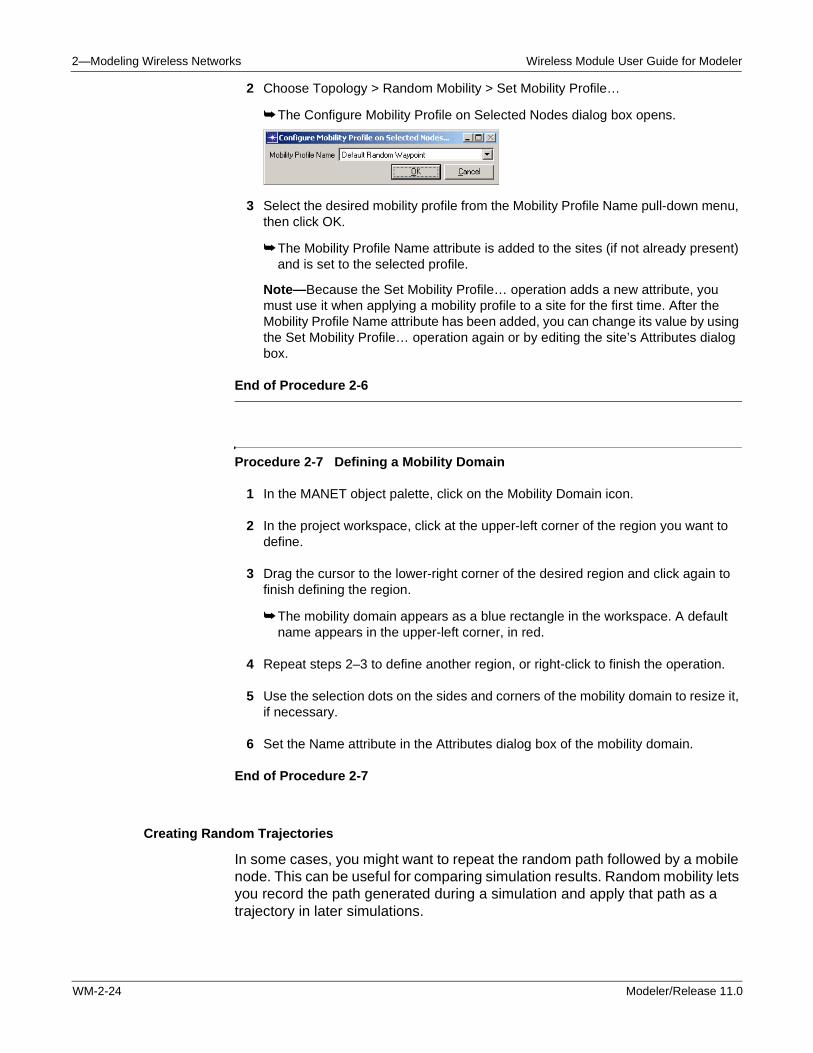
2 Choose Topology > Random Mobility > Set Mobility Profile…

➥ The Configure Mobility Profile on Selected Nodes dialog box opens.

3 Select the desired mobility profile from the Mobility Profile Name pull-down menu, then click OK.

➥ The Mobility Profile Name attribute is added to the sites (if not already present) and is set to the selected profile.

Note—Because the Set Mobility Profile… operation adds a new attribute, you must use it when applying a mobility profile to a site for the first time. After the Mobility Profile Name attribute has been added, you can change its value by using the Set Mobility Profile… operation again or by editing the site’s Attributes dialog box.


Procedure 2-7 Defining a Mobility Domain

1 In the MANET object palette, click on the Mobility Domain icon.

2 In the project workspace, click at the upper-left corner of the region you want to define.

3 Drag the cursor to the lower-right corner of the desired region and click again to finish defining the region.

➥ The mobility domain appears as a blue rectangle in the workspace. A default name appears in the upper-left corner, in red.

4 Repeat steps 2–3 to define another region, or right-click to finish the operation.

5 Use the selection dots on the sides and corners of the mobility domain to resize it, if necessary.

6 Set the Name attribute in the Attributes dialog box of the mobility domain.


Creating Random Trajectories

In some cases, you might want to repeat the random path followed by a mobile node. This can be useful for comparing simulation results. Random mobility lets you record the path generated during a simulation and apply that path as a trajectory in later simulations.



If the Record Trajectory attribute of a random mobility profile is set to Enabled, Modeler will create trajectory files during simulation, one file for each site using that profile. Each trajectory file contains a list of the coordinates traversed by a site. The trajectory files are named <project-scenario>-<node_name>.trj and placed in the default model directory.

Although you can assign these trajectories to sites exactly as you would a trajectory you created yourself, there is a faster way, as described in Procedure 2-8.

Procedure 2-8 Assigning Random Trajectories to One or More Sites

1 Select the mobile sites to which you want to apply random trajectories. To apply trajectories to all mobile sites, leave them all unselected.

2 Choose Topology > Random Mobility > Set Trajectory Created From Random Mobility…

➥ For each selected site (or all sites), Modeler looks for a random trajectory from the current scenario and, if found, applies it to the corresponding site.


Direct Manipulation of Position Attributes

Note—This section applies only to Modeler.

If a trajectory is specified for a mobile site, the path of that site is predetermined for the entire simulation. However, if no trajectory is specified, the site’s position can be directly updated by any process during simulation. A mobile site’s x position and y position attributes specify its location in its parent subnetwork. A mobile site’s altitude attribute specifies its elevation relative to sea level, the underlying terrain, or the parent subnetwork (depending on the site’s altitude modeling attribute setting). A change to one of these attributes will effect an immediate change in the location of the mobile site.

Typically, one of two techniques is employed to dynamically change the location of a mobile site. In both cases, a user-defined process is responsible for modifying the position attributes of a mobile site. The first technique is a centralized approach, in which one process is responsible for updating the positions of all of the mobile sites in a network model. Often this process resides within a site specially designated as a central control site. The second technique



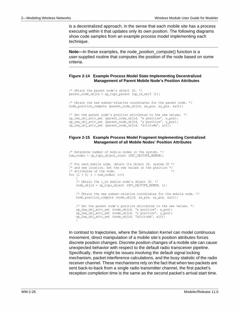
is a decentralized approach, in the sense that each mobile site has a process executing within it that updates only its own position. The following diagrams show code samples from an example process model implementing each technique.

Note—In these examples, the node_position_compute() function is a user-supplied routine that computes the position of the node based on some criteria.

Figure 2-14 Example Process Model State Implementing Decentralized Management of Parent Mobile Node’s Position Attributes

/* Obtain the parent node’s object ID. */parent_node_objid = op_topo_parent (op_id_self ());

/* Obtain the new subnet-relative coordinates for the parent node. */node_position_compute (parent_node_objid, &x_pos, &y_pos, &alt);

/* Set the parent node’s position attributes to the new values. */op_ima_obj_attr_set (parent_node_objid, “x position”, x_pos);op_ima_obj_attr_set (parent_node_objid, “y position”, y_pos);op_ima_obj_attr_set (parent_node_objid, “altitude”, alt);

Figure 2-15 Example Process Model Fragment Implementing Centralized Management of all Mobile Nodes’ Position Attributes

/* Determine number of mobile nodes in the system. */num_nodes = op_topo_object_count (OPC_OBJTYPE_NDMOB);

/* For each mobile node, obtain its object ID, system ID *//* and new location. Set the new values in the position *//* attributes of the node. */for (i = 0; i < num_nodes; i++)

{/* Obtain the i_th mobile node’s object ID. */node_objid = op_topo_object (OPC_OBJTYPE_NDMOB, i);

/* Obtain the new subnet-relative coordinates for the mobile node. */node_position_compute (node_objid, &x_pos, &y_pos, &alt);

/* Set the parent node’s position attributes to the new values. */op_ima_obj_attr_set (node_objid, “x position”, x_pos);op_ima_obj_attr_set (node_objid, “y position”, y_pos);op_ima_obj_attr_set (node_objid, “altitude”, alt);}

In contrast to trajectories, where the Simulation Kernel can model continuous movement, direct manipulation of a mobile site’s position attributes forces discrete position changes. Discrete position changes of a mobile site can cause unexpected behavior with respect to the default radio transceiver pipeline. Specifically, there might be issues involving the default signal locking mechanism, packet interference calculations, and the busy statistic of the radio receiver channel. These mechanisms rely on the fact that when two packets are sent back-to-back from a single radio transmitter channel, the first packet’s reception completion time is the same as the second packet’s arrival start time.



This is based on two propagation delay calculations: the first packet’s propagation delay at the end of its transmission and the second packet’s propagation delay at the beginning of its transmission. If these propagation delays are not the same, then two back-to-back packets will incorrectly appear to overlap each other or to have a gap between them.

As two sites move closer together or farther apart during transmission, the propagation delay of the radio signal will correspondingly change. Thus, at the beginning and end of transmission of one packet, the start and end propagation delays for a packet sent from a mobile site can be different. If the difference in propagation delays is not accounted for, then the overlap or gap behavior occurs with back-to-back packets.

The default radio transceiver pipeline does not prevent the overlap or gap behavior in the case of discrete position changes. This is due to the fact that the Simulation Kernel cannot predict the future location of a mobile site without use of a trajectory. In this case, the Simulation Kernel sets the end of transmission propagation distance in a packet’s TDA OPC_TDA_RA_END_DIST to the same value as the start of transmission propagation distance, found in the packet’s TDA OPC_TDA_RA_START_DIST. The default radio pipeline stage that computes the propagation delays, dra_propdel.ps.c, uses these values and therefore returns the same result for both delays.

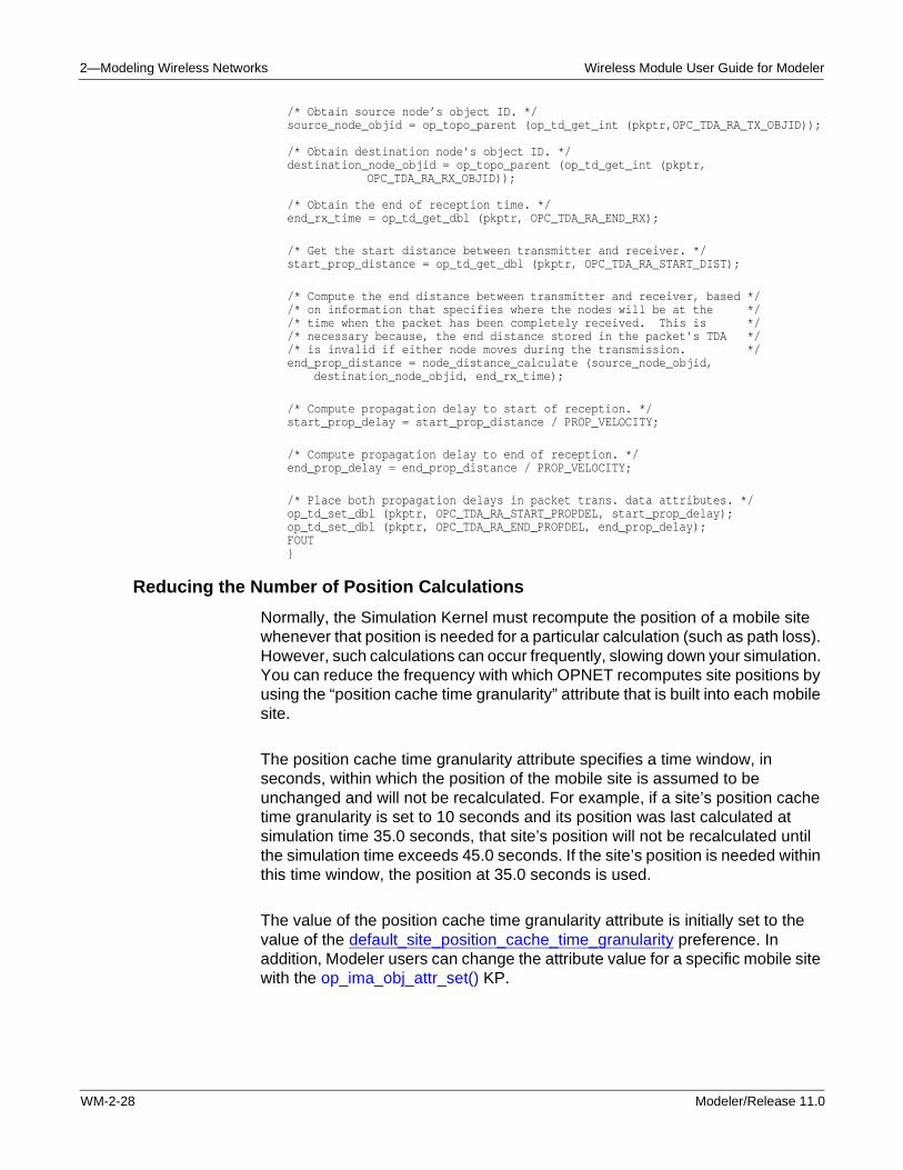
One solution is to replace the default radio pipeline stage with another that will correctly compute the end of transmission propagation delay. The following code is an example pipeline stage that correctly calculates this delay. It is assumed that the procedure node_distance_calculate() returns the distance in meters between the specified sites at the specified time. If such a procedure is not possible, then some other solution that handles the default signal locking mechanism, packet interference calculations, and the busy statistic of the radio receiver channel issues should be used instead.

Figure 2-16 Example Propagation Delay Radio Pipeline Stage

/* mobile_propdel.ps.c */ /* Propagation delay model for radio link Transceiver Pipeline */

#include <opnet.h>/* propagation velocity of radio signal (m/s) */define PROP_VELOCITY 3.0E+08

#if defined (__cplusplus)extern “c”#endif

voidmobile_propdel (Packet *pkptr)

{double start_prop_delay, end_prop_delay;double start_prop_distance, end_prop_distance;Objid source_node_objid, destination_node_objid;double end_rx_time;

/** Compute the propagation delays separating the **//** radio transmitter from the radio receiver. **/FIN (mobile_propdel (pkptr))



/* Obtain source node’s object ID. */source_node_objid = op_topo_parent (op_td_get_int (pkptr,OPC_TDA_RA_TX_OBJID));

/* Obtain destination node’s object ID. */destination_node_objid = op_topo_parent (op_td_get_int (pkptr,

OPC_TDA_RA_RX_OBJID));

/* Obtain the end of reception time. */end_rx_time = op_td_get_dbl (pkptr, OPC_TDA_RA_END_RX);

/* Get the start distance between transmitter and receiver. */start_prop_distance = op_td_get_dbl (pkptr, OPC_TDA_RA_START_DIST);

/* Compute the end distance between transmitter and receiver, based *//* on information that specifies where the nodes will be at the *//* time when the packet has been completely received. This is *//* necessary because, the end distance stored in the packet’s TDA *//* is invalid if either node moves during the transmission. */end_prop_distance = node_distance_calculate (source_node_objid,

destination_node_objid, end_rx_time);

/* Compute propagation delay to start of reception. */start_prop_delay = start_prop_distance / PROP_VELOCITY;

/* Compute propagation delay to end of reception. */end_prop_delay = end_prop_distance / PROP_VELOCITY;

/* Place both propagation delays in packet trans. data attributes. */op_td_set_dbl (pkptr, OPC_TDA_RA_START_PROPDEL, start_prop_delay);op_td_set_dbl (pkptr, OPC_TDA_RA_END_PROPDEL, end_prop_delay);FOUT}

Reducing the Number of Position Calculations

Normally, the Simulation Kernel must recompute the position of a mobile site whenever that position is needed for a particular calculation (such as path loss). However, such calculations can occur frequently, slowing down your simulation. You can reduce the frequency with which OPNET recomputes site positions by using the “position cache time granularity” attribute that is built into each mobile site.

The position cache time granularity attribute specifies a time window, in seconds, within which the position of the mobile site is assumed to be unchanged and will not be recalculated. For example, if a site’s position cache time granularity is set to 10 seconds and its position was last calculated at simulation time 35.0 seconds, that site’s position will not be recalculated until the simulation time exceeds 45.0 seconds. If the site’s position is needed within this time window, the position at 35.0 seconds is used.

The value of the position cache time granularity attribute is initially set to the value of the default_site_position_cache_time_granularity preference. In addition, Modeler users can change the attribute value for a specific mobile site with the op_ima_obj_attr_set() KP.



When selecting a value for either the position cache time granularity attribute or the default_site_position_cache_time_granularity preference, you should consider the rate at which the site’s position changes (its speed) and how much position inaccuracy is tolerable in your simulation.



Statistics in a Wireless Network

The Wireless Module provides some additional statistic support to help you evaluate wireless networks.

Collection Mode

The Wireless Module adds an additional collection mode for statistics:

• Glitch removal—collects only the last value generated at any given simulation time.

Coupled Node Statistic Probes

Coupled node statistic probes record information relating to a particular object’s activity with respect to its interaction with another object. Only a small number of statistics in OPNET support coupled probing; currently, these are all statistics of the radio receiver channel object. The coupling mechanism allows the probe to focus only on the performance of a link between the receiver channel and a particular transmitter elsewhere in the model. For example, a coupled node statistic probe allows the received power statistic of a receiver channel to measure only the power of the signal incident upon the receiver from a specific transmitter. The same statistics can be collected using an ordinary node statistic probe, in which case it will represent the received power from any transmitter, whenever activity occurs. In other words, the coupled node statistic probe provides selectivity.

Coupled node statistic probes can capture the following radio receiver channel statistics:

• signal-to-noise ratio

• bit error rate

• packet error rate

• bit errors per packet

• received power

More information about coupled statistic probes and their attributes appear in Coupled Node Statistic Probe Object on page WM-5-102.

Automatic Animation Probes

The Wireless Module allows you to capture animation of mobile and satellite node movement within a subnetwork, in addition to packet flows.



Custom Animation Probes

For Modeler users creating custom animation probes, the Radio Transceiver Pipeline can issue animation directives. These are similar to those issued by the standard transceiver pipelines, as described in Animation Probes on page MC-11-13 of the Modeling Concepts manual.

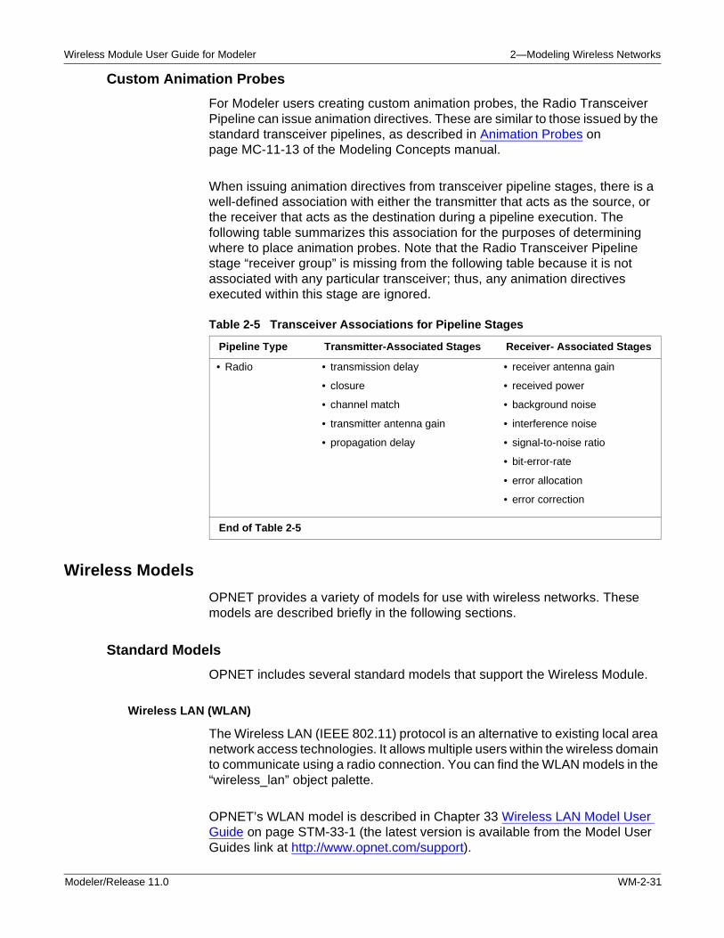
When issuing animation directives from transceiver pipeline stages, there is a well-defined association with either the transmitter that acts as the source, or the receiver that acts as the destination during a pipeline execution. The following table summarizes this association for the purposes of determining where to place animation probes. Note that the Radio Transceiver Pipeline stage “receiver group” is missing from the following table because it is not associated with any particular transceiver; thus, any animation directives executed within this stage are ignored.

Wireless Models

OPNET provides a variety of models for use with wireless networks. These models are described briefly in the following sections.

Standard Models

OPNET includes several standard models that support the Wireless Module.

Wireless LAN (WLAN)

The Wireless LAN (IEEE 802.11) protocol is an alternative to existing local area network access technologies. It allows multiple users within the wireless domain to communicate using a radio connection. You can find the WLAN models in the “wireless_lan” object palette.

OPNET’s WLAN model is described in Chapter 33 Wireless LAN Model User Guide on page STM-33-1 (the latest version is available from the Model User Guides link at http://www.opnet.com/support).

Table 2-5 Transceiver Associations for Pipeline Stages

Pipeline Type Transmitter-Associated Stages Receiver- Associated Stages

• Radio • transmission delay

• closure

• channel match

• transmitter antenna gain

• propagation delay

• receiver antenna gain

• received power

• background noise

• interference noise

• signal-to-noise ratio

• bit-error-rate

• error allocation

• error correction

End of Table 2-5


http://www.opnet.com/support


Jammer Models

OPNET provides three basic jamming sources that can be used in wireless network models. The three models—a pulsed jammer, a frequency-swept jammer, and a fixed-frequency single-band jammer—are available on the “jammers” object palette. The jammers are provided as node and process models in the <reldir>/models/std/jammers directory. These models are described in Jammer Model Descriptions on page WM-12-1.

Antenna Models

OPNET provides antenna patterns for selected antennas from several vendors. These are stored in the <reldir>/models/vendor_models/antenna_models directory. Documentation about these antennas is available from the contributed models section of the OPNET web site (in the OPNET software, choose Help > Web - Contributed Models, then search for “antenna patterns”).

Specialized Models

OPNET offers a growing number of specialized models for specific wireless modeling needs. These models include:

• Wireless LAN (WLAN)

• Mobile Ad Hoc Networks (MANET)

— Ad Hoc On Demand Distance Vector Routing (AODV)

— Dynamic Source Routing (DSR)

— Optimized Link State Routing (OLSR)

— Temporally-Ordered Routing Algorithm (TORA)

• Universal Mobile Telecommunications System (UMTS)

For information about these models, refer to the documentation provided with the model or to the model guides (located in the Specialized Model User Guides manual and from the Model User Guides link at http://www.opnet.com/support).


http://www.opnet.com/support

modeling wireless networks

Documents