modeling the effect of clay drapes on pumping test
TRANSCRIPT
Accepted Manuscript
Modeling the effect of clay drapes on pumping test response in a cross-bedded
aquifer using multiple-point geostatistics
Marijke Huysmans, Alain Dassargues
PII: S0022-1694(12)00380-0
DOI: http://dx.doi.org/10.1016/j.jhydrol.2012.05.014
Reference: HYDROL 18232
To appear in: Journal of Hydrology
Received Date: 2 March 2012
Revised Date: 2 May 2012
Accepted Date: 7 May 2012
Please cite this article as: Huysmans, M., Dassargues, A., Modeling the effect of clay drapes on pumping test response
in a cross-bedded aquifer using multiple-point geostatistics, Journal of Hydrology (2012), doi: http://dx.doi.org/
10.1016/j.jhydrol.2012.05.014
This is a PDF file of an unedited manuscript that has been accepted for publication. As a service to our customers
we are providing this early version of the manuscript. The manuscript will undergo copyediting, typesetting, and
review of the resulting proof before it is published in its final form. Please note that during the production process
errors may be discovered which could affect the content, and all legal disclaimers that apply to the journal pertain.
1
Modeling the effect of clay drapes on pumping test response in a 2
cross-bedded aquifer using multiple-point geostatistics 3
4
Marijke Huysmans(1)
(corresponding author) and Alain Dassargues(1,2)
5
6
(1) Katholieke Universiteit Leuven 7
Applied Geology and Mineralogy 8
Department of Earth and Environmental Sciences 9
Celestijnenlaan 200 E 10
3001 Heverlee 11
Belgium 12
Tel: +32 16 32 64 49 13
Fax: +32 16 32 29 80 14
E-mail: [email protected] 15
16
(2) Université de Liège 17
Hydrogeology and Environmental Geology 18
Department of Architecture, Geology, Environment, and Civil Engineering (ArGEnCo) 19
B.52/3 Sart-Tilman 20
4000 Liège 21
Belgium 22
23
24

2
Abstract 25
This study investigates whether fine-scale clay drapes can cause an anisotropic pumping test 26
response at a much larger scale. A pumping test was performed in a sandbar deposit 27
consisting of cross-bedded units composed of materials with different grain sizes and 28
hydraulic conductivities. The measured drawdown values in the different observation wells 29
reveal an anisotropic or elliptically-shaped pumping cone. The major axis of the pumping 30
ellipse is parallel with the strike of cm to m-scale clay drapes that are observed in several 31
outcrops. To determine (1) whether this large-scale anisotropy can be the result of fine-scale 32
clay drapes and (2) whether application of multiple-point geostatistics can improve 33
interpretation of pumping tests, this pumping test is analysed with a local 3D groundwater 34
model in which fine-scale sedimentary heterogeneity is modelled using multiple-point 35
geostatistics. To reduce CPU and RAM demand of the multiple-point geostatistical simulation 36
step, edge properties indicating the presence of irregularly-shaped surfaces are directly 37
simulated. Results show that the anisotropic pumping cone can be attributed to the presence 38
of the clay drapes. Incorporating fine-scale clay drapes results in a better fit between observed 39
and calculated drawdowns. These results thus show that fine-scale clay drapes can cause an 40
anisotropic pumping test response at a much larger scale and that the combined approach of 41
multiple-point geostatistics and cell edge properties is an efficient method for integrating fine-42
scale features in larger scale models. 43
44
Keywords: Multiple-point geostatistics; Groundwater Flow; Heterogeneity; Pumping test; 45
Upscaling; Cross-bedding 46
47
Highlight 1: Fine-scale clay drapes can cause anisotropic pumping test response at larger 48
scale 49

3
Highlight 2: An approach using multiple-point geostatistics and edge properties is proposed 50
Highlight 3: Incorporating fine-scale clay drapes results in a better fit of drawdowns 51
52
53
54

4
1. Introduction 55
Clay drapes are thin irregularly-shaped layers of low-permeability material that are often 56
observed in different types of sedimentary deposits (Reineck and Singh 1973). Their 57
thicknesses are often only a few centimetres (Houthuys 1990; Stright 2006). Despite their 58
limited thicknesses, several studies indicate that they may influence subsurface fluid flow and 59
solute transport at different scales (Ringrose et al. 1993; Willis and White 2000; Morton et al. 60
2002; Mikes 2006; Stright 2006; Li and Caers 2011; Huysmans and Dassargues 2009). It 61
seems that structural heterogeneity (such as clay drapes) at fine scale might yield anisotropy 62
at large scale, whereas ―random" heterogeneity may yield an isotropic behavior at large scale. 63
However, many studies show that the effect of fine-scale heterogeneity is limited to fine 64
scales and averaged out on larger scales and that consequently the type of geological 65
heterogeneity that needs to be taken into account depends on the scale of the problem under 66
consideration (Schulze-Makuch and Cherkauer 1998; Schulze-Makuch et al. 1999; Beliveau 67
2002; Neuman 2003; Eaton 2006). Van den Berg (2003) found for example that anisotropy 68
caused by lamination is small compared to the influence of larger scale heterogeneities so that 69
these sedimentary structures only cause anisotropy on a smaller scale. It is therefore unclear 70
whether centimeter-scale clay drapes can influence groundwater flow and solute transport at 71
scales exceeding the meter-scale. This study therefore investigates whether fine-scale clay 72
drapes can cause an anisotropic pumping test response at a much larger scale. This study is 73
based on measured drawdown values from a pumping that reveal an anisotropic or elliptical-74
shaped pumping cone: the major axis of the pumping ellipse is parallel with the strike of the 75
centimetre to meter-scale clay drapes that are observed and measured in several outcrops and 76
quarries. This study quantitatively investigates whether this large-scale anisotropy can be the 77
result of fine-scale clay drapes. 78
79
5
It is very difficult to incorporate clay drapes in aquifer or reservoir flow models, because of 80
their small size and the complexity of their shape and distribution. In standard upscaling 81
approaches (Renard and de Marsily 1997; Farmer 2002), the continuity of the clay drapes is 82
not preserved (Stright 2006). Multiple-point geostatistics is a technique that has proven to be 83
very suitable for simulating the spatial distribution of such complex structures (Strebelle 84
2000; Strebelle 2002; Caers and Zhang 2004; Hu and Chugunova 2008; Huysmans and 85
Dassargues, 2009; Comunian et al. 2011; dell’Arciprete et al. 2012). Multiple-point 86
geostatistics was developed for modelling subsurface heterogeneity as an alternative to 87
variogram-based stochastic approaches that are generally not well suited to simulate complex, 88
curvilinear, continuous, or interconnected structures (Koltermann and Gorelick 1996; Fogg et 89
al. 1998; Journel and Zhang 2006). Multiple-point geostatistics overcomes the limitations of 90
variogram by directly inferring the necessary multivariate distributions from training images 91
(Guardiano and Srivastava 1993; Strebelle and Journel 2001; Strebelle 2000; Strebelle 2002; 92
Caers and Zhang 2004; Hu and Chugunova 2008). In this way, multiple-point geostatistics 93
provides a simple mean to integrate a conceptual geological model in a stochastic simulation 94
framework (Comunian et al., 2011). In the field of groundwater hydrology, application of 95
multiple-point geostatistics to modeling of groundwater flow and transport in heterogeneous 96
media has become an active research topic in recent years. Feyen and Caers (2006) apply the 97
method to a synthetic two-dimensional case to conclude that the method could potentially be a 98
powerful tool to improve groundwater flow and transport predictions. Several recent studies 99
apply the method to build realistic (hydro)geological models based on field observations on 100
geological outcrops and logs (Huysmans et al. 2008; Ronayne et al. 2008; Huysmans and 101
Dassargues 2009; Bayer et al. 2011; Comunian et al. 2011; Le Coz et al. 2011; dell’Arciprete 102
et al. 2012). In large-scale three-dimensional grids multiple-point geostatistics may be 103
computationally very intensive. Several studies focus on improved implementations of the 104
6
multiple-point statistics techniques to make the algorithms more powerful and 105
computationally efficient (e.g., Mariethoz et al. 2010; Straubhaar et al. 2011). Huysmans and 106
Dassargues (2011) developed the method of ―direct multiple-point geostatistical simulation of 107
edge properties‖ which enables simulating thin irregularly-shaped surfaces with a smaller 108
CPU and RAM demand than the conventional multiple-point statistical methods. This method 109
has been applied on simple test cases (Huysmans and Dassargues 2011) and the present study 110
is the first to apply the method of ―direct multiple-point geostatistical simulation of edge 111
properties‖ to a full-scale three-dimensional groundwater model. In this way, this study 112
investigates whether the combined approach of using multiple-point geostatistics and edge 113
properties is an efficient and valid method for integrating fine-scale features in larger scale 114
models. 115
116
A last scientific goal of this paper is to determine the added benefits of explicitly 117
incorporating clay drape presence for inverse modelling of pumping tests. Several authors 118
have shown that incorporating heterogeneity can result in improved correspondence between 119
calculated and observed hydraulic heads (e.g., Herweijer 1996; Lavenue and de Marsily 2001; 120
Kollet and Zlotnik 2005; Ronayne et al. 2008; Harp and Vesselinov 2011). However, some 121
authors show that incorporating additional data about heterogeneity does not always result in 122
better calibration (e.g., Hendricks Franssen and Stauffer 2005). This paper quantifies the 123
change in calibration error when clay drapes are incorporated in groundwater flow models. 124
125
126
2. Material and methods 127
The methodology followed in this study consists of the following steps. First, field data are 128
obtained in an extensive field campaign mapping sedimentary heterogeneity and fine-scale air 129

7
permeability. Secondly, a training image displaying clay drape occurence is constructed based 130
on the geological and hydrogeological field data obtained from this field campaign. Thirdly, 131
this training image with small pixel size is converted into an upscaled edge training image 132
which is used as input training image to perform multiple-point SNESIM (Single Normal 133
Equation SIMulation) simulations. The SNESIM algorithm (Strebelle 2002) allows borrowing 134
multiple-point statistics from the training image to simulate multiple realizations of facies 135
occurrence. SNESIM is a pixel-based sequential simulation algorithm that obtains multiple-136
point statistics from the training image, exports it to the geostatistical numerical model, and 137
anchors it to the actual subsurface hard and soft data. In this study, the resulting simulations 138
indicate at which cell edges horizontal or vertical clay drapes are present. This information is 139
incorporated in a local 3D groundwater model of the pumping test site by locally adapting 140
vertical leakance values and by locally inserting horizontal flow barriers. All hydraulic 141
parameters including the clay drapes properties are calibrated using the measured drawdown 142
time series in six observation wells. 143
144
2.1 Geological setting 145
The pumping test site is situated in Bierbeek near Leuven (Belgium) as shown in Figure 1. 146
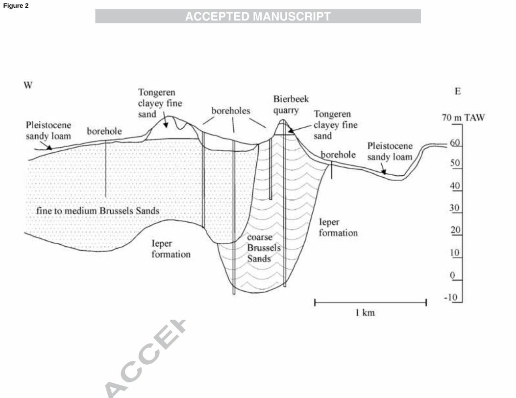
The subsurface geology in this area consists of a 4m-thick cover of sandy loam from 147
Pleistocene age, 35m of Middle-Eocene Brussels Sands and 12 m of low permeable Early-148
Eocene Ieper Clay (Figure 2). At the pumping test site the Brussels Sands aquifer acts as an 149
unconfined aquifer. All pumping and observation wells of the pumping test are screened in 150
the Brussels Sands. The Brussels Sands formation is an early Middle-Eocene shallow marine 151
sand deposit in Central Belgium (Fig. 1). Its geological features are extensively covered in 152
Houthuys (1990) and Houthuys (2011). This aquifer is a major source of groundwater in 153
Belgium and was studied at the regional scale by Peeters et al. (2010). The most interesting 154
8
feature of these sands in terms of groundwater flow and transport is the complex geological 155
heterogeneity originating in its depositional history. The Brussels Sands are a tidal sandbar 156
deposit. Its deposition started when a strong SSW-NNE tidal current in the early Middle-157
Eocene produced longitudinal troughs, that were afterwards filled by sandbar deposits. In 158
these sandbar deposits, sedimentary features such as cross-bedding, mud drapes and 159
reactivation surfaces are abundantly present (Houthuys 1990; Houthuys 2011). The 160
orientation of most of these structures is related to the NNE-orientation of the main tidal flow 161
during deposition. 162
163
2.2 Pumping test 164
In February 1993, a pumping test was performed in Bierbeek (Belgium) under the authority of 165
the company TUC RAIL N.V. in the framework of high-speed train infrastructure works. One 166
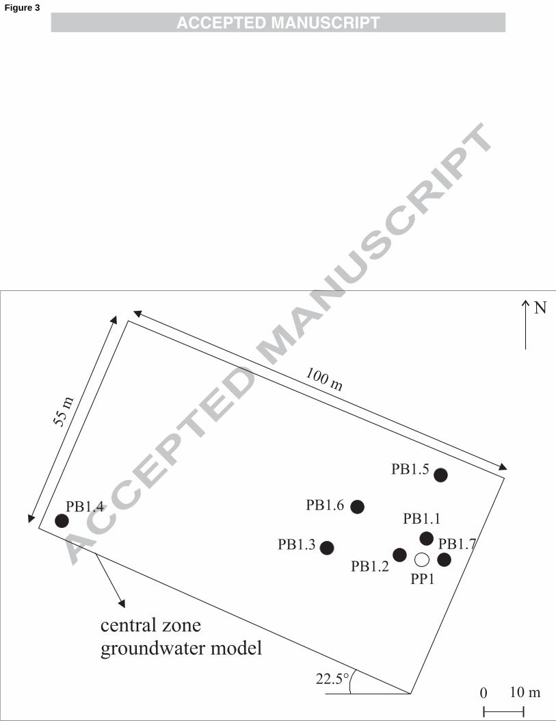
pumping well (PP1) and six observations wells were drilled in the 35m-thick coarse facies of 167
the Brussels Sands (Figure 3). The observation wells are situated between 4m and 75m from 168
the pumping well and are located in different orientations. Before pumping the water table 169
was at 49.8 m. During the pumping test, there was 72 hours of pumping in well PP1 with a 170
flow rate of 2120 m³/day. Water level in six observation wells was continuously monitored 171
during pumping and during an additional 24 hours of recovery after pumping. The pumping 172
test was interpreted by inverse modelling using a numerical method described in Lebbe and 173
De Breuck (1995). This analysis showed that the best calibration was obtained assuming 174
horizontal anisotropy in the coarse facies of the Brussels Sands. The maximal horizontal 175
hydraulic conductivity was found to be 28.3 m/day while the minimal horizontal hydraulic 176
conductivity was 13.4 m/day. The principal direction of maximal horizontal hydraulic 177
conductivity corresponds to N 115°48’ E (TUC RAIL N.V., 1993). This principal orientation 178
9
is exactly perpendicular to the SSW-NNE orientation of the main tidal flow during deposition 179
and the mud drapes in the Brussels Sands. 180
181
182
2.3 In situ mapping and measurement of clay drape properties 183
The Brussels Sands outcrops in the Bierbeek quarry are used as an analog for the Brussels 184
Sands found in the subsurface at the pumping test site. This quarry is located at approximately 185
500 m from the pumping test site (Figure 1). This outcrop of approximately 1200 m² was 186
mapped in detail with regard to the spatial distribution of sedimentary structures and 187
permeability in Huysmans et al. (2008). A total of 2750 cm-scale air permeability 188
measurements were carried out in situ on different faces of the Bierbeek quarry to 189
characterize the spatial distribution of permeability. From the hydrogeological point of view 190
in the present study, the main interest lies in the occurrence and geometry of structures with 191
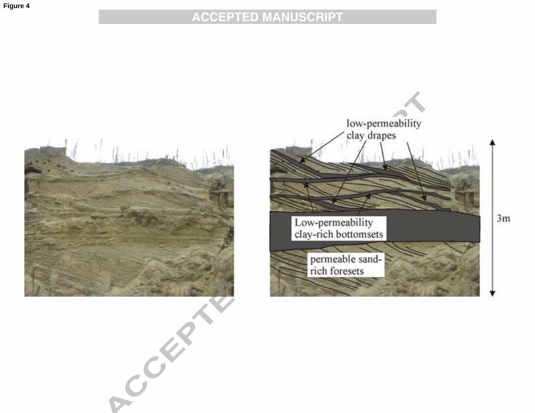
high and low hydraulic conductivity. In this perspective, the Brussels Sands can be regarded 192
as consisting of horizontal permeable sand layers of approximately 1m thick intercalated by 193
horizontal low-permeable clay-rich bottomsets and inclined low-permeable clay drapes. 194
Figure 4 shows a field picture and a geological interpretation of the typical clay-sand patterns 195
in the Bierbeek quarry. More details about the spatial distribution of the fine-scale 196
sedimentary structures and measured permeability in the Brussels Sands can be found in 197
Huysmans et al. (2008). 198
199
2.4 Training image construction 200
The observed spatial patterns of clay drape occurrence are explicitly represented in a training 201
image. Training images are essential to multiple-point geostatistics. In multiple-point 202
geostatistics, "training images" are used to characterize the patterns of geological 203

10
heterogeneity. A training image is an explicit grid-based representation of the expected 204
geological patterns. In the simulation step, patterns are borrowed from the training image and 205
reproduced in the simulation domain. (Guardiano and Srivastava 1993; Strebelle and Journel, 206
2001; Caers and Zhang 2004). More information about the theory behind multiple-point 207
geostatistics can be found in Strebelle (2000) and Strebelle (2002). Description of the 208
different multiple-point algorithms can be found in the following papers: SNESIM (Strebelle 209
2002; Liu 2006), FILTERSIM (Zhang et al. 2006; Wu et al. 2008), SIMPAT (Arpat and Caers 210
2007), HOSIM (Mustapha and Dimitrakopoulos 2010) and the Direct Sampling method 211
(Mariethoz et al. 2010). 212
213
In this study, a two-dimensional fine-scale training image of clay and sand occurrence of the 214
Brussels Sands was constructed based on the in situ mapping in the Bierbeek quarry. In the 215
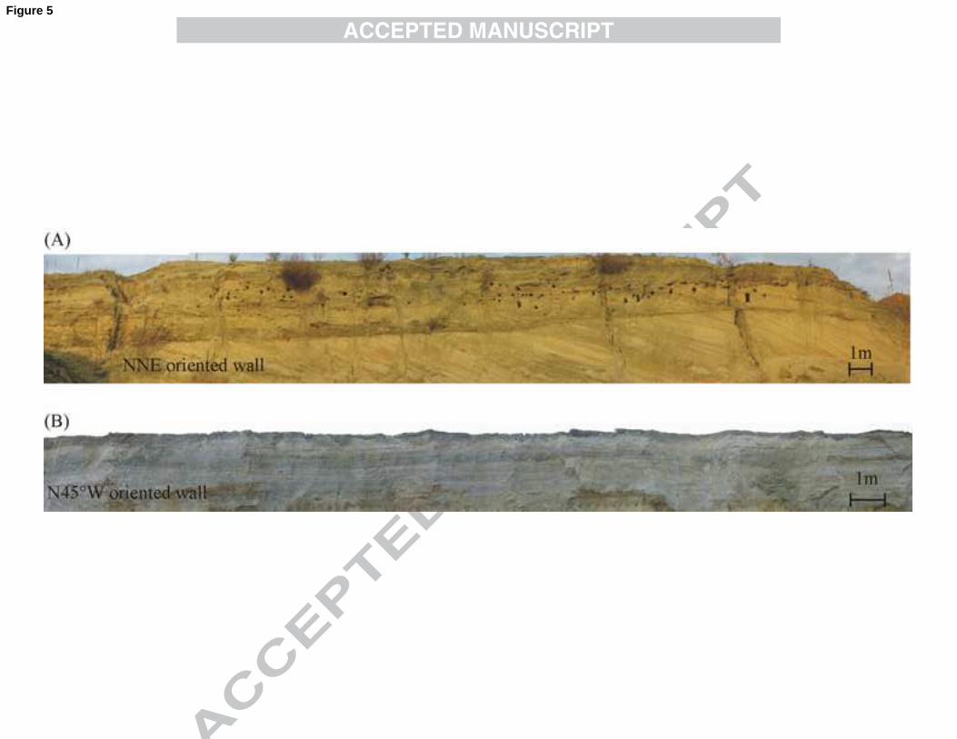
third dimension perpendicular to the 2D training image, layering and clay drapes are very 216
continuous as shown on figure 5 which shows quarry wall pictures in the NNE-direction and 217
the perpendicular orientation. While the picture of the NNE-oriented face displays cross-218
bedding and inclined mud drapes, the picture of the perpendicular face shows continuous 219
horizontal layering (Figure 5). Therefore all layers and sedimentary structures are assumed to 220
be continuous in that direction. The incorporation of 3D simulations based on several 2D 221
training images in different directions following the approaches discussed in Comunian et al. 222
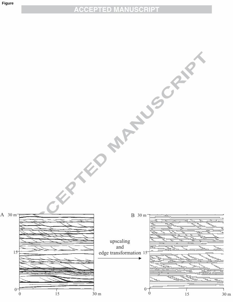
(2012) could be interesting future work. The two-dimensional fine-scale training image along 223
the NNE-direction (Figure 6) shows an alternation of sand-rich and clay-rich zones. More 224
details about construction of this training image can be found in Huysmans and Dassargues 225
(2009). This training image will be used in section 2.6 where multiple-point statistics are 226
borrowed from this training image to simulate realizations of clay drape occurrence to be used 227
as input for the local groundwater flow model. 228
11
229
2.5 Groundwater flow model 230
The groundwater flow model is a three-dimensional local model of 600m x 600 m x 30.4m 231
including all pumping and observation wells from the pumping test in Bierbeek described in 232
section 2.2. The size of the model in the horizontal direction was chosen to be 600 m since 233
analysis of the pumping test data showed that no drawdown is measured at 300 m from the 234
pumping well (TUCRAIL N.V., 1993). The model is oriented along the N22.5°E direction 235
which is parallel to the direction of the main geological structures and the main anisotropy 236
axis of the observed drawdowns from the pumping test. The top of the Ieper Clay deposits 237
represents the impermeable bottom of the model due to the low permeability of this unit 238
(Huysmans and Dassargues, 2006). The top of the model corresponds to an elevation of 49.8 239
m, which corresponds to the initial groundwater level before pumping. This means that only 240
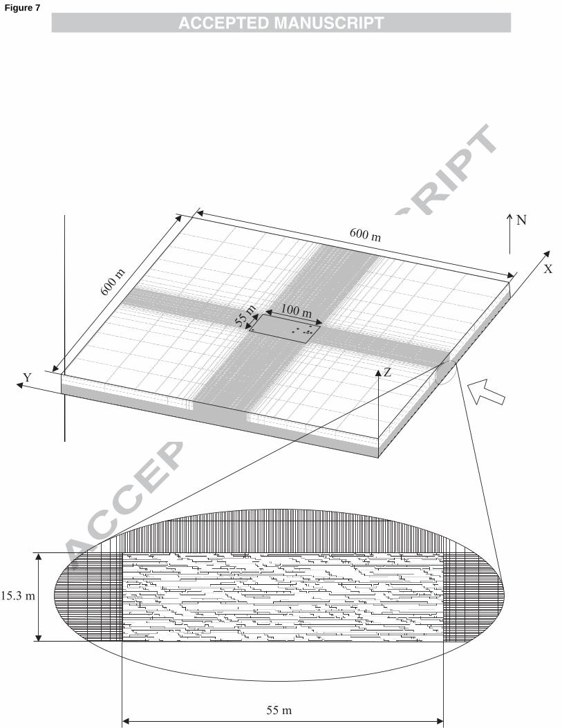
one geological layer is present in the model, i.e., the Brussels Sands. The model consists of a 241
central inner zone of 55m x 100m x 15.3m including all well screens and an outer zone 242
(Figure 7). This inner zone consists of 51 cells in the x-direction, 183 cells in the y-direction 243
and 51 layers. In the central inner zone where all the well screens are situated, a very small 244
grid cell size of 0.3m x 0.3m x 0.3m is adopted so that individual clay drapes can be explicitly 245
incorporated in the model in this zone. In the outer zone, larger grid cell sizes between 0.45m 246
and 82m in the horizontal direction and layer thicknesses between 3m and 6m are chosen. For 247
numerical reasons, the dimensions of the grid cells do not exceed 1.5 times the dimensions of 248
their neighboring cells. The total model consists of 213 cells in the x-direction, 361 cells in 249
the y-direction and 54 layers. The total number of grid cells in the model is thus 4,152,222 250
cells. The model is run in transient conditions with a total time length of 4510 minutes 251
subdivided into 99 time intervals. Piezometric heads are prescribed at the lateral boundaries of 252
all model layers. In the pumping well PP1, a pumping rate of 2120 m³/day is applied during 253
12
72 hours. Initial hydraulic conductivity and storage parameters were taken from a previous 254
interpretation (TUCRAIL N.V., 1993) and calibrated afterwards. A total of 594 observed 255
heads measured in six observation wells (Figure 3) from two minutes after the start of 256
pumping until 240 minutes after stopping of pumping are available for calibration. The 257
differential equations describing groundwater flow are solved by PMWIN (Chiang and 258
Kinzelbach 2001), which is a pre- and post-processor for MODFLOW (McDonald and 259
Harbaugh 1988), using a block-centered, finite-difference, method. 260
261
Two model variants are run and calibrated separately. First, a homogeneous and horizontally 262
isotropic model without clay drapes is run. In this model, different values for horizontal and 263
vertical hydraulic conductivity are allowed, but no anisotropy of hydraulic conductivity in the 264
horizontal direction is introduced. Calibration is performed for adapting values of horizontal 265
hydraulic conductivity, vertical hydraulic conductivity and specific storage. The second 266
model incorporates a random clay drape realization as described in section 2.6. In this model, 267
calibration of the following additional parameters is performed: clay drape thickness and clay 268
drape hydraulic conductivity in model layers 4 to 54 and anisotropy factor of shallow layers 1 269
to 3 in which clay drapes are not explicitly incorporated. In layers 1 to 3 clay drapes are not 270
explicitly incorporated since these belong to the outer zone of the model The spatial 271
distribution of the clay drapes is not changed during calibration. Storage is assumed identical 272
in the sand and the clay drapes. In this model, the only heterogeneity and anisotropy of 273
hydraulic conductivity is related to the presence of clay drapes. Background hydraulic 274
conductivity of layers 4 to 54 is homogeneous and isotropic so that the effect of clay drapes 275
on hydraulic heads can be determined without influence of other heterogeneity or anisotropy 276
effects. By comparing the results of these two model variants, the effects of clay drapes on the 277
piezometric depression cone and on the calibration results can be quantified. This approach of 278
13
comparing a heterogeneous model with a homogeneous equivalent was for example also 279
applied in Mariethoz et al. (2009). For both models, a two-step calibration procedure is 280
adopted. First, a sensitivity analysis and trial-and-error subjective calibration is performed and 281
second, the optimal model from manual calibration is further calibrated using PEST (Doherty 282
et al. 1994). The sensitivity analysis consists of varying the adjustable parameters (horizontal 283
hydraulic conductivity, vertical hydraulic conductivity, specific storage and clay drape 284
parameters) and assessing their effect on simulated drawdowns. 285
286
2.6 Clay drapes simulation using multiple-point geostatistical simulation of edge 287
properties 288
289
In order to incorporate clay drapes showing patterns similar to the training image of Figure 6 290
(left) in the groundwater flow model, the technique of direct multiple-point geostatistical 291
simulation of edge properties (Huysmans and Dassargues 2011) is used. This technique was 292
designed to simulate thin complex surfaces such as clay drapes with a smaller CPU and RAM 293
demand than the conventional multiple-point statistical methods. Instead of pixel values, edge 294
properties indicating the presence of irregularly-shaped surfaces are simulated using multiple-295
point geostatistical simulation algorithms. The training image is upscaled by representing clay 296
drapes as edge properties between cells instead of representing them as objects consisting of 297
several cells. The concept of the edge of a flow model and the associated edge properties was 298
introduced in the work of Stright (2006) as an additional variable. The edge properties are 299
assigned to the cell faces. The cell property used in this study is the presence of clay drapes 300
along cell faces. More details about the method can be found in Huysmans and Dassargues 301
(2011). Figure 6 shows how the fine-scale pixel-based training image (left) is converted into 302
an upscaled edge-based training image (right). The fine-scale training image has a grid cell 303
14
size of 0.05 m and represents the clay drapes as consisting of pixels with a different pixel 304
value than the background material. The upscaled edge-based training image has a grid cell 305
size of 0.30 m and represents the clay drapes as edge properties that indicate the presence of 306
clay drapes along the edges of all grid cells. 307
308
In this study, the upscaled 30 m by 30 m training image from Figure 6 (right) is used as input 309
to SNESIM from SGeMS (Remy et al. 2009) to simulate clay drape realizations to be 310
imported in the inner central zone of the model where individual clay drapes are incorporated. 311
Vertical 2D realizations of 54.9m by 15.3m are generated. Figure 7 shows a random clay 312
drape realization that is incorporated in the groundwater flow model. 313
314
The realizations of clay drape presence can be imported in the groundwater flow code 315
PMWIN using the Horizontal-Flow Barrier (HBF) package and the vertical leakance array 316
(VCONT array). The HBF package simulates thin vertical low-permeability geological 317
features, which impede horizontal groundwater flow. They are situated on the boundaries 318
between pairs of adjacent cells in the finite-difference grid (Hsieh and Freckleton, 1993). A 319
horizontal-flow barrier is defined by assigning the barrier direction, which indicates the cell 320
face where the barrier is located, and barrier hydraulic conductivity divided by the thickness 321
of the barrier (Chiang and Kinzelbach, 2001). Horizontal edges are inserted into PMWIN by 322
adapting vertical leakance (VCONT array) between two model layers. The VCONT matrix 323
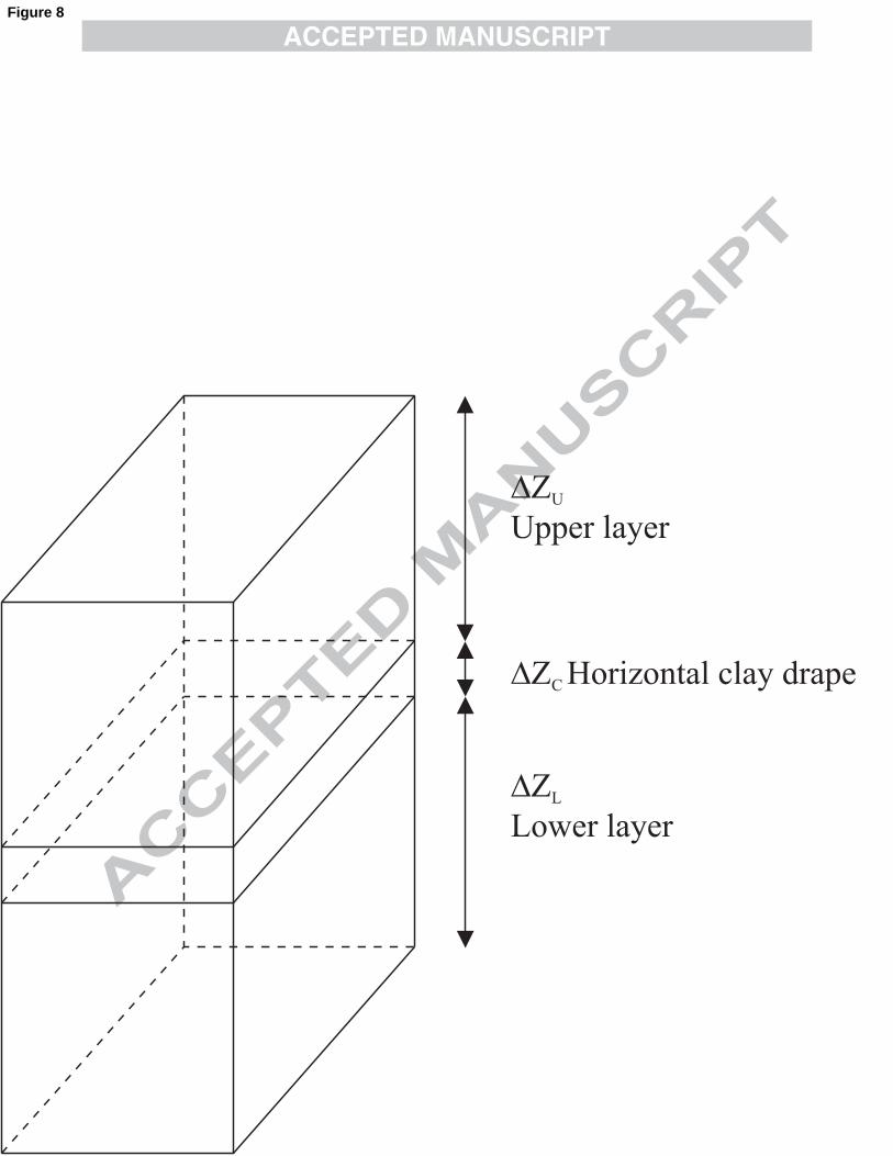
for every model layer is calculated as 324
2
u c l
z z zu c l
VCONTz z z
K K K
(1) 325
where K is hydraulic conductivity, Δz is thickness and u, c and l respectively represent the 326
upper layer, semi-confining unit and lower layer as indicated on figure 8. In case a horizontal 327
15
edge is present in a model cell, the edge is inserted in the model as a semi-confining unit. 328
Initially, it is assumed that all clay drapes in the groundwater flow model have a thickness of 329
0.02 m and a hydraulic conductivity of 0.283 m/d. As mentioned previously, these values are 330
optimized during calibration. 331
332
3. Results 333
Figures 9 and 10 show the resulting model outputs from the homogeneous model and the clay 334
drape model. For both models, automatic calibration using PEST did not result in lower 335
calibration errors, possibly as a result of the large size (4,152,222 grid cells) and complexity 336
of the models. Manual calibration was apparently able to identify a good local minimum, 337
possibly due to the small number of calibrated variables. In the homogeneous and horizontally 338
isotropic model, the best calibration results were obtained with the following set of calibrated 339
parameter values: horizontal hydraulic conductivity of 22.2 m/day, vertical hydraulic 340
conductivity of 4.8 m/day and specific storage of 3 x 10⁻⁵
m-1
. In the clay drape model, the 341
best calibration results were obtained with the following set of calibrated parameter values: 342
horizontal hydraulic conductivity of 23 m/day vertical hydraulic conductivity of 4 m/day, 343
specific storage of 3 x 10⁻⁵
m-1
and a clay drape parameter (hydraulic conductivity of drapes 344
divided by drape thickness) with values between 0.175 and 9.905 day-1
. This clay drape 345
parameter varied between the different sublayers of the inner zone of the model reflecting the 346
alteration between layers with thicker or less permeable clay drapes and layers with thinner or 347
more permeable clay drapes. In every layer, a single clay drape parameter was assigned, thus 348
not allowing spatial variation of the clay drape parameter within the model layers. 349
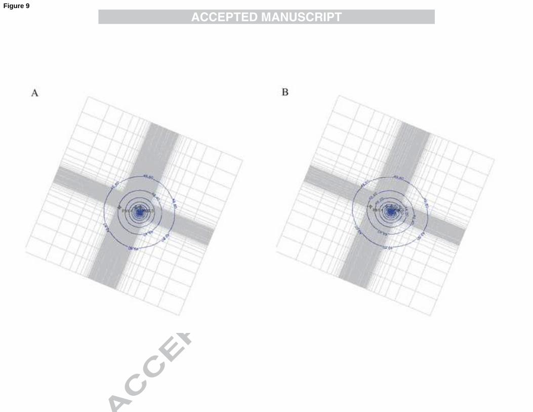
Figure 9 shows piezometric maps at z = 27 m amsl, i.e., located at the depth of the centre of 350
the pumping well screen, for (1) the homogeneous and horizontally isotropic model and (2) 351
the clay drape model. Figure 9A shows circular hydraulic head contours indicating an 352
16
isotropic piezometric pumping depression cone resulting from the homogeneity and isotropy 353
of hydraulic conductivity in the horizontal direction. Figure 9B shows the hydraulic head 354
contours for the second model which incorporates clay drapes. These contours are elliptical 355
demonstrating an anisotropic pumping depression cone. The vertical clay drapes cause 356
bending of the hydraulic head contours. Since no other K heterogeneity than the clay drape 357
presence is incorporated in the model, these results show that anisotropic pumping cones at 358
large-scale can be attributed to the presence of fine-scale clay drapes. 359
360
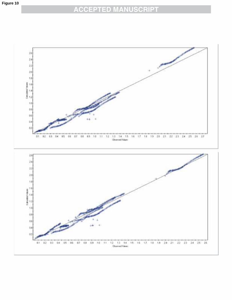
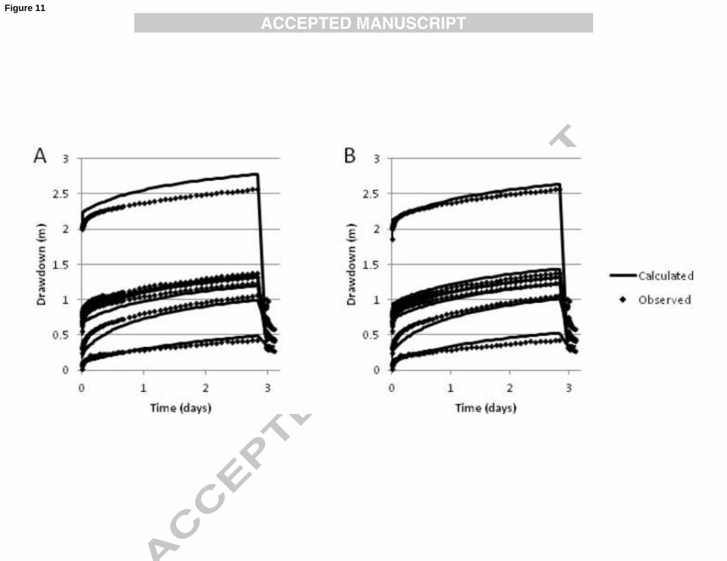
Figure 10 shows calculated versus observed drawdown graphs for (1) the homogeneous and 361
horizontally isotropic model variant and (2) the clay drape model variant. Figure 11 shows 362
calculated and observed drawdown versus time for (1) the homogeneous and horizontally 363
isotropic model variant and (2) the clay drape model variant The error variance for the 364
isotropic model is 1.24 E-2 m², while the error variance for the clay drape model is as low as 365
7.292E-3 m². The residual mean of the homogeneous and isotropic model is -3.08 E-2 m, 366
while the residual mean for the clay drape model is -2.12 E-2 m. Correlation coefficient 367
between observed and simulated drawdowns increases from 0.9906 (homogeneous/isotropic 368
model) to 0.9916 (clay drape model). Incorporating the clay drapes thus results in a better 369
fitting between calculated and observed drawdown values for this pumping test. Especially 370
the larger drawdowns are better reproduced in the clay drape model. This is most obvious on 371
figure 11 which shows that time behaviour is generally well reproduced by the model but that 372
larger drawdowns are better reproduced in the clay drape model. These large drawdowns are 373
measured in observation well PB1.2 which is located close to the pumping well (Figure 3). In 374
the clay drape model, a clay drape is present in the pumped layer between the pumping well 375
and observation well PB1.2 which acts as a flow barrier between those two wells. The 376

17
presence of this barrier results in a better reproduction of the measured drawdowns by the 377
model. 378
379
4. Discussion and conclusion 380
This study has investigated the effect of fine-scale clay drapes on pumping test response. For 381
this purpose, spatial distribution and geometry of clay drapes observed in a cross-bedded 382
aquifer were explicitly incorporated in a local groundwater model of a pumping test site. Clay 383
drape parameters were calibrated in order to reproduce hydraulic head measurements 384
observed during a pumping test. Best calibration results were obtained with a zoned clay 385
drape parameter or drape leakage coefficient, defined as hydraulic conductivity of drapes 386
divided by drape thickness, with values between 0.175 and 9.905 day-1
. If the clay drape 387
thickness is assumed to be 0.02 m, this means that hydraulic conductivity of the clay drapes is 388
between 0.0035 m/day (= 4.05x10⁻⁸
m/s) and 0.1981 m/day (= 2.29x10⁻⁶
m/s). These values lie 389
in the hydraulic conductivity interval of silt and silty sand respectively according to Fetter 390
(2001), so these values are realistic and are certainly not chosen unrealistically low. This 391
implies that the anisotropic pumping cone can be reproduced and explained with realistic 392
values for clay drape thickness and hydraulic conductivity andthat fine-scale clay drapes can 393
cause an anisotropic pumping test response at a much larger scale. 394
395
Incorporating clay drapes in groundwater models is challenging since they are often irregular 396
curvilinear three-dimensional surfaces which may display a very complex spatial distribution. 397
In this paper, a combined approach of multiple-point geostatistics and edge properties was 398
used to incorporate the clay drapes in the flow model. Clay drapes were represented as grid 399
cell edge properties instead of representing them by pixels. This allowed modelling with a 400
larger grid cell size and thus a smaller CPU and RAM demand. A realistic spatial distribution 401
18
of clay drape occurence was simulated using multiple-point geostatistics based on a field-402
based training image. This combined approach of multiple-point geostatistics and edge 403
properties has shown to be an efficient and valid approach since realistic spatial patterns and 404
geometry of the clay drapes can be preserved in the model without having to represent each 405
clay drape by pixels. 406
407
In order to determine the added value of explicitly incorporating clay drape presence in the 408
flow model for pumping test interpretation, the model was also compared with a 409
homogeneous and isotropic model calibrated on the same pumping test data. Incorporating the 410
clay drapes resulted in a better fit between calculated and observed drawdown values than the 411
homogeneous model. 412
413
414
Acknowledgements 415
The authors wish to acknowledge the Fund for Scientific Research – Flanders for providing a 416
Postdoctoral Fellowship to the first author. We thank TUCRAIL for providing the pumping 417
test data. 418
419
References 420
Arpat, G.B. and J. Caers (2007) Conditional simulation with patterns, Mathematical Geology 421
39(2): 177-203. 422
423
Bayer, P., Huggenberger, P., Renard, P. and A. Comunian (2011) Three-dimensional high 424
resolution fluvio-glacial aquifer analog: Part 1: Field study, J. Hydrol. 405(1-2), 1-9. 425
426
19
Beliveau, D. (2002), Reservoir heterogeneity, geostatistics, horizontal wells, and black jack 427
poker, AAPG Bulletin 86 (10), 1847– 1848. 428
429
Caers, J., and T. Zhang (2004), Multiple-point geostatistics: a quantitative vehicle for 430
integrating geologic analogs into multiple reservoir models, In: Integration of outcrop and 431
modern analog data in reservoir models, AAPG memoir, vol 80, pp 383–394. 432
433
Chiang, W., and W. Kinzelbach (2001), 3D-groundwater modeling with PMWIN, Springer, 434
Berlin. ISBN 3-540-67744-5. 435
436
Comunian, A., Renard, P., Straubhaar, J. and Bayer P. (2011) Three-dimensional high 437
resolution fluvio-glacial aquifer analog – Part 2: Geostatistical modeling, Journal of 438
Hydrology 405(1-2): 10-23. 439
440
Comunian, A., Renard, P., Straubhaar, J. (2012) 3D multiple-point statistics simulation using 441
2D training images. Computers and Geosciences 40, 49-65. 442
443
dell’Arciprete, D., Bersezio, R., Felletti, F., Giudici, M., Comunian, A., Renard, P. (2012), 444
Comparison of three geostatistical methods for hydrofacies simulation: a test on alluvial 445
sediments, Hydrogeol J 20, 299-311. 446
447
Doherty, J., Brebber, L., and P. Whyte (1994), PEST - Model-independent parameter 448
estimation. User’s manual. Watermark Computing. Australia. 449
450
20
Eaton, T.T. (2006), On the importance of geological heterogeneity for flow simulation, Sed 451
Geol 184, 187–201. 452
453
Farmer, C.L. (2002), Upscaling: a review, Int J Num Meth Fluids 40(1-2), 63-78. 454
455
Feyen, L. And J. Caers (2006), Quantifying geological uncertainty for f low and transport 456
modeling in multi-modal heterogeneous formations, Adv Water Resour 29(6), 912-929. 457
Fetter, C.W. (2001), Applied hydrogeology, Prentice-Hall, New Yersey, 598 p. 458
459
Fogg, G.E., Noyes, C.D. and S.F. Carle (1998), Geologically based model of heterogeneous 460
hydraulic conductivity in an alluvial setting, Hydrogeol J 6(1), 131–143. 461
462
Guardiano, F. And M. Srivastava(1993), Multivariate geostatistics: beyond bivariate 463
moments, In: Soares A (ed) Geostatistics-Troia. Kluwer Academic, Dordrecht. 464
465
Harp, D.R. and V.V. Vesselinov (2011), Identification of Pumping Influences in Long-Term 466
Water Level Fluctuations, Ground Water 49(3), 403-414. 467
468
Hendricks Franssen, H.-J. and F. Stauffer (2005), Inverse stochastic estimation of well 469
capture zones with application to the Lauswiesen site (Tübingen, Germany), In Renard P., 470
Demougeot-Renard H. and Froidevaux R. (Eds), Geostatistics for Environmental 471
Applications, Proceedings of the Fifth European Conference on Geostatistics for 472
Environmental Applications, Springer-Verlag, Berlin, Heidelberg. 473
474
Herweijer, J. (1996), Constraining uncertainty of groundwater flow and transport models 475
21
using pumping tests, in Calibration and Reliability in Groundwater Modelling, pp. 473 476
482, IAHS Publ., 237. 477
478
Houthuys, R. (1990), Vergelijkende studie van de afzettingsstruktuur van getijdenzanden uit 479
het Eoceen en van de huidige Vlaamse banken, Aardkundige Mededelingen 5, Leuven 480
University Press, p. 137. 481
482
Houthuys, R. (2011), A sedimentary model of the Brussels Sands, Eocene, Belgium, 483
Geologica Belgica 14(1-2), 55-74. 484
485
Hsieh, P.A., and J.R. Freckleton (1993), Documentation of a computer program to simulate 486
horizontal-flow barriers using the U.S. Geological Survey’s modular three-dimensional finite-487
difference ground water flow model, U.S. Geological Survey Open File Report 92-477. 488
489
Hu, L.Y., and T. Chugunova (2008), Multiple-point geostatistics for modeling subsurface 490
heterogeneity: a comprehensive review, Water Resour Res 44:W11413, 491
doi:10.1029/2008WR006993. 492
493
Huysmans, M., and A. Dassargues (2006), Hydrogeological modeling of radionuclide 494
transport in low permeability media: a comparison between Boom Clay and Ypresian Clay, 495
Env Geol, 50 (1), 122-131 496
497
Huysmans, M., and A. Dassargues (2009), Application of multiple-point geostatistics on 498
modeling groundwater flow and transport in a cross-bedded aquifer, Hydrogeol J 17(8), 1901-499
1911 500
22
501
Huysmans, M., and A. Dassargues (2011), Direct multiple-point geostatistical simulation of 502
edge properties for modelling thin irregularly-shaped surfaces, Math Geosci 43 (5), 521-536 503
504
Huysmans, M., Peeters, L., Moermans, G., and A. Dassargues (2008), Relating small-scale 505
sedimentary structures and permeability in a cross-bedded aquifer, J Hydrol 361, 41-51 506
507
Journel, A. and T. Zhang (2006), The necessity of a multiple-point prior model, Math Geol 508
38(5), 591–610. 509
510
Kollet, S.J. and V.A. Zlotnik (2005), Influence of aquifer heterogeneity and return flow on 511
pumping test data interpretation, J Hydrol 300(1-4), 267-285 512
513
Koltermann, C.E. and S. Gorelick (1996), Heterogeneity in sedimentary deposits: a review of 514
structure imitating, process-imitation, and descriptive approaches, Water Resour Res 32(9), 515
2617–2658. 516
517
Lavenue, M. and G. de Marsily (2001), Three-dimensional interference test interpretation in a 518
fractured aquifer using the pilot point inverse method, Water Resour Res 37(11), 2659-2675 519
520
Lebbe, L. and W. Debreuck (1995), Validation of an inverse numerical model for 521
interpretation of pumping tests and a study of factors influencing accuracy of results, J Hydrol 522
172(1-4), 61-85 523
524
23
Le Coz, M., Genthon, P., and P.M. Adler (2011), Multiple-point statistics for modeling facies 525
heterogeneities in a porous medium: the Komadugu-Yobe Alluvium, Lake Chad Basin, Math. 526
Geosci. 43, 861-878. 527
528
Li, H.M. and J. Caers (2011), Geological modelling and history matching of multi-scale flow 529
barriers in channelized reservoirs: methodology and application, Petroleum Geoscience 17(1): 530
17-34. 531
532
Liu, Y. (2006), Using the Snesim program for multiple-point statistical simulation, Comput 533
Geosci 32(10):1544–1563 534
535
Mariethoz, G., Renard, P., Cornaton, F., Jacquet, O. (2009), Truncated plurigaussian 536
simulations to characterize aquifer heterogeneity, Ground Water 47(1), 13-24. 537
538
Mariethoz, G., Renard, P. and J. Straubhaar (2010), The Direct Sampling method to perform 539
multiple-point geostatistical simulations, Water Resour Res, 46, W11536, DOI: 540
10.1029/2008WR007621 541
542
McDonald, M.G., and A.W. Harbaugh (1988), A modular three-dimensional finite-difference 543
ground-water flow model, Technical report USGS, Reston, VA 544
545
Mikes, D. (2006), Sampling procedure for small-scale heterogeneities (crossbedding) for 546
reservoir modeling, Mar. Petrol. Geol. 23 (9-10), 961-977. 547
548
24
Morton, K., Thomas, S., Corbett, P., and D. Davies (2002), Detailed analysis of probe 549
permeameter and vertical inteference test permeability measurements in a heterogeneous 550
reservoir, Petrol. Geosci. 8, 209-216. 551
552
Mustapha, H. and R. Dimitrakopoulos (2010), High-order stochastic simulation of complex 553
spatially distributed natural phenomena, Math Geosci 42:457–485. 554
555
Neuman, S.P. (2003), Multifaceted nature of hydrogeologic scaling and its interpretation, 556
Reviews of Geophysics 41 (3), 4.1– 4.31. 557
558
Peeters, L., Fasbender, D., Batelaan, O. and A. Dassargues (2010), Bayesian Data Fusion for 559
water table interpolation: incorporating a hydrogeological conceptual model in kriging, Water 560
Resour Res 46(8), DOI:10.1029/2009WR008353 561
562
Reineck, H.-E. and I. B. Singh (1973), Depositional sedimentary environments, Springer-563
Verlag, Berlin, New York, 439 p. 564
565
Remy, N., Boucher, A. And J. Wu (2009) Applied Geostatistics with SGeMS – a user’s guide, 566
Cambridge University Press, New York, 264 p. 567
568
Renard, Ph. and G. de Marsily (1997), Calculating equivalent permeability: a review, Adv 569
Water Resour 20 (5-6): 253-278 570
571
25
Ringrose, P.S., Sorbie, K.S., Corbett, P. W. M. and J.L. Jensen (1993) Immiscible flow 572
behaviour in laminated and cross-bedded sandstones, Journal of Petroleum Science and 573
Engineering 9 (2): 103-124. 574
575
Ronayne, M.J., Gorelick, S.M., and J. Caers (2008,) Identifying discrete geologic structures 576
that produce anomalous hydraulic response: An inverse modeling approach, Water Resour 577
Res 44(8), DOI: 10.1029/2007WR006635 578
579
Schulze-Makuch, D. and D.S. Cherkauer (1998) Variations in hydraulic conductivity with 580
scale of measurement during aquifer tests in heterogeneous, porous carbonate rocks, 581
Hydrogeol J 6 (2), 204– 215. 582
583
Schulze-Makuch, D., Carlson, D.A., Cherkauer, D.S., and P. Malik (1999), Scale depency of 584
hydraulic conductivity in heterogeneous media, Ground Water 37(6), 904-919 585
586
J. Straubhaar, P. Renard, G. Mariethoz, R. Froidevaux, O. Besson (2011), An improved 587
parallel multiple-point algorithm using a list approach, Math. Geosci. 43(3), 305–328. 588
589
Strebelle, S. (2000), Sequential simulation drawing structures from training images, Doctoral 590
dissertation, Stanford University. 591
592
Strebelle, S. and A.G. Journel (2001) Reservoir modeling using multiple-point statistics. 593
SPE Annual Technical conference and Exhibition, New Orleans, Sept. 30 – Oct. 3, 2001, 594
SPE # 71324. 595
596
26
Strebelle, S. (2002), Conditional simulation of complex geological structures using multiple-597
point statistics, Math Geol 34:1–22. 598
599
Stright, L., (2006) Modeling, Upscaling and History Matching Thin, Irregularly-Shaped Flow 600
Barriers; A Comprehensive Approach for Predicting Reservoir Connectivity, SPE Paper 601
106528. 602
603
TUC RAIL N.V. (1993), Studie van de invloed van de tunnel voor de HSL op het 604
groundwater van Bierbeek, internal report. 605
606
Van den Berg, E.H. (2003), The impact of primary sedimentary structures on groundwater 607
flow—a multi-scale sedimentological and hydrogeological study in unconsolidated eolian 608
dune deposits, PhD Thesis, Vrije Universiteit Amsterdam, 196 pp.. 609
610
Willis, B.J. and C.D. White (2000), Quantitative outcrop data for flow simulation, J. 611
Sediment. Res. 70, 788-802. 612
613
Wu, J., Boucher, A., and T. Zhang (2008), SGeMS code for pattern simulation of continuous 614
and categorical variables: FILTERSIM, Comput Geosci 34:1863–1876. 615
616
Zhang, T., Switzer, P., Journel, A.G. (2006), Filter-based classification of training image 617
patterns for spatial simulation, Math Geol 38:63–80 618
619
27
Figure captions 620
621
Figure 1 Map of Belgium showing Brussels Sands outcrop and subcrop area (shaded part) 622
(modified after Houthuys (1990) and inset showing the location of the pumping test site and 623
the Bierbeek quarry 624
625
Figure 2 Geological EW-profile through the study area, modified after Houthuys (1990) 626
627
Figure 3 Pumping test configuration showing the pumping well (white circle) and 628
observation wells (black circles) and the orientation and delineation of the central inner zone 629
of the local groundwater model. Observation well PB1.1 is not screened in the Brussels Sands 630
and is therefore not used in this study. 631
632
Figure 4 Raw (left) and interpreted (right) field picture, showing foresets, bottomsets and 633
clay drapes in the Brussels Sands observed in the Bierbeek quarry 634
635
Figure 5 (A) Photomosaic of Bierbeek quarry wall in NNE direction showing cross-bedding 636
and quasi-horizontal clay-rich bottomsets. Height of quarry wall is approximately 4–5 m and 637
(B) photomosaic of N45°W oriented Bierbeek quarry wall showing continuous horizontal 638
layers. Length of quarry wall shown on picture is approximately 22 m. 639
640
Figure 6 (A) Vertical two-dimensional training image of 30 m by 30 m in NNE direction: 641
sand facies (white), clay-rich facies (black) modified from Huysmans and Dassargues (2009) 642
and (B) the corresponding edge training image modified from Huysmans and Dassargues 643
(2011) 644
28
645
Figure 7 Groundwater flow model grid and edge realization 646
647
Figure 8 Grid configuration used for the calculation of VCONT in the presence of a 648
horizontal clay drape between two cells (modified after Chiang and Kinzelbach 2001) 649
650
Figure 9 Piezometric maps at z = 27 m corresponding to the central level of the pumping well 651
screen, for (A) the homogeneous and horizontally isotropic model and (B) the clay drape 652
model showing drawdown after two days 653
654
Figure 10 Calculated versus observed drawdown graphs for (1) the homogeneous and 655
horizontally isotropic model variant and (2) the clay drape model variant 656
657
Figure 11 Calculated and observed drawdown versus time for (A) the homogeneous and 658
horizontally isotropic model variant and (B) the clay drape model variant 659
660

PB1.5
PB1.6PB1.1
PB1.3
PB1.4
PB1.2
PB1.7
PP1
0 10 m
N
central zonegroundwater model
100 m
55 m
22.5°
Figure 3
00 15 30 m
15
30 m
00 15 30 m
15
30 m
upscalingand
edge transformation
A B
Figure
600 m
600
m
X
Y Z
N
100 m
55m
55 m
15.3 m
Figure 7
DZU
Upper layer
DZL
Lower layer
DZC Horizontal clay drape
Figure 8

Highlight 1: Small-scale clay drapes can cause anisotropic pumping test response at larger
scale
Highlight 2: An approach using multiple-point geostatistics and edge properties is proposed
Highlight 3: Incorporating small-scale clay drapes results in a better fit of drawdowns