modeling salinity affects in relation to soil fertility and crop yield; · 2007-04-25 ·...
TRANSCRIPT
Modeling Salinity Affects in Relation to Soil Fertility and Crop Yield;
A Case Study of Nakhon Ratchasima, Nong Suang District, Thailand
Ram Dular Yadav March, 2005

Modeling Salinity Affects in Relation to Soil Fertility and Crop Yield;
A Case Study of Nakhon Ratchasima, Nong Suang District, Thailand
by
Ram Dular Yadav Thesis submitted to the International Institute for Geo-information Science and Earth Observation in partial fulfilment of the requirements for the degree of Master of Science in Geo-information Science and Earth Observation, Specialisation: (Soil information for sustainable land management) Thesis Assessment Board Dr. D. G. Rossiter (Chairperson) Dr. Victor Jetten (External Examiner) Mr. Valentijn Venus (Internal Examiner) Dr. Abbas Farshad (Main Supervisor) Dr. Dhrub P. Shrestha (Co-Supervisor)
INTERNATIONAL INSTITUTE FOR GEO-INFORMATION SCIENCE AND EARTH OBSERVATION
ENSCHEDE, THE NETHERLANDS

Disclaimer This document describes work undertaken as part of a programme of study at the International Institute for Geo-information Science and Earth Observation. All views and opinions expressed therein remain the sole responsibility of the author, and do not necessarily represent those of the institute.

DEDICATED
TO MY LATE
FATHER AND MOTHER FOR THEIR LOVING CARE


MODELING SALINIITY AFFECTS IN RELATION TO SOIL FERTILITY AND CROP YIELD
R.D. Yadav, MSc Thesis, 2005 i
Abstract
Abstract
Globally, high soil salinity is acknowledged as one of the major threats to agriculture. Geology, geomorphology and anthropogenic activities have shown to cause and/or accelerate salinization in different parts of the worlds. Increasing population and their demand causes changes in landuse/ cover that determine the changes in salinity levels. Out of the several causes, geology, geomorphology, groundwater depth and salinity, deforestation, human intervention and weather pattern are the main causes of salinization in the research site. These with low soil fertility severely affect the crop yield. To tackle these threats, the research is conducted with the general objective “To model salinity affects in relation with fertility parameters and crop yield in the both feature- and geographic- spaces, by applying relevant simulation and GIS-oriented models to track down the crop growth in order to predict the yield under various degrees of salinity influence” with specific objectives of this thesis was: (1) to study soil salinity and soil fertility parameters in geopedological units; (2) to establish the relationship between soil salinity and crop productivity;(3) to establish and evaluate the relationship between soil salinity (EC) and soil organic matter content; (4) assessing crop productivity using CropSyst, PS 12 and GIS oriented model, and (5) making a comparison between the applied models, followed up by some recommendations
Some selected measured soil salinity and fertility variables (EC, pH, CEC and OM) were used to estimate their variation in geopedologic units at “relief type” and at landscape levels, and also their spatial variation and dependency to estimate the area affected by salinity. Different crop growth simulation models (CropSyst and PS123) were used to assess crop yield considering different degree of salinity, taking soil fertility and other crop physiologic properties, climate and management factors into account. The relationships of the estimated parameters i.e. between variables, among interrelated variables; were also established keeping objective of the research in mind. The relevant images was processed and classified to prepare landuse/cover map in order to use for yield mapping. Their relationship and interrelationships were also examined. All these analyses were done using classical statistics technique in SPSS, Curve, and Excel; geostatistics techniques and image classification facilities of ILWIS 3.2 environment. Sensitivity analysis for salinity in land suitability for different crops were determined with the respective model (crop growth, SMCE) and relationship of outputs were established and compared Soil salinity and soil fertility varied significantly within and between geopedologic units at “relief type” and landscape level. Selected salinity and soil fertility parameters did not show significant relationship but there was significant relationship among the soil fertility parameters. Moving average gave best interpolation result in salinity and fertility modelling and indicator kriging could be used for salinity hotspot mapping. PS123 simulates crop yield that correlates significantly with farmers yield. This was not true for the case of CropSyst. Both models simulate crop yield with different degree of salinity (sensitivity analysis). Crop yield with different degree of salinity in relation to soil fertility can be predicted by crop growth model the result of which is integrated in GIS environment for further manipulations. Also, suitability map of different crops based on land qualities can be modelled using GIS for instance SMCE.

MODELING SALINIITY AFFECTS IN RELATION TO SOIL FERTILITY AND CROP YIELD
R.D. Yadav, MSc Thesis, 2005 ii
Acknowledgements
I extend my sincere thanks to The Netherlands Fellowship Programme (Nuffic) for financial support without which this degree was not possible in ITC. I am grateful to the Nepal government, Ministry of Agriculture and Department of Agriculture for nominating me for this course. I would like to thank Mr Sadanad Jaishy for his initiative and support. I would like to extend my special gratitude to my supervisor Dr. Abbas Farshad for his guidance throughout my M.Sc. research work. It was not possible to shape the research without his guidance. I also owe Dr. Dhrub Pika Shrestha my co- supervisor an affectionate appreciation for his valuable guidance during fieldwork that made it possible to obtain appropriate data. Sincerely, I thank Dr. David Rossitter for his valuable and critical comments that enhance my capability to come up with result oriented research. I am also grateful to Ir. R.J. (Rob) Sporry for his valuable comment during my midterm presentation. During the field work in Thailand, many institution and people have supported me and extended my sincere thanks to them. I am much indebt of LDD staff Mr.Anukul Suchinai for providing me all kinds of support required during the field work. I would also like to thank Mr. Chatchai, Mr.Thuwin (Win), Miss Panikorn (Jang), Ms Yampong (Bee) and Mr. Suparee (Driver) who helped me in data collection and household survey in different villages and also thanks to all the villagers for providing me relevant information for my research work. I would like to thank Mrs Parida, Dr. Arunin, Dr. Runawarga and Mr. Somsak for providing me necessary data and literature for my research work. Also, special thanks go to staffs of laboratory of Khon Kaen for timely analyzing the soil which were important input data of my research work. I thank all the staff at ITC. I feel privileged to be the recipient of the many new things that I have learnt. Staffs at the ITC library deserve special mention. They were always eager to help, and entertained my many requests for inter-library loans. Over the course of the last one and half years, I have made many friends from all over the world. In this respect, ITC is truly a special place. Most importantly, I remain grateful to Mr. Roger Nelson for his support in running the CropSyst model and also clarification of some quarries. Many thanks go to my cluster mates Ha (Vietnam), Benson (Tanzania), Benjamin (Ghana), Daniel (Ghana), Pattaraporn (Thailand) and Harssema (Ethiopia) for their support during the project work. I would like to thank all Nepalese friends for providing me homely environment and support during the period of stay in the Netherlands. Special thanks go to Mr. C. Joshi, Mr. A. Mathema, Mr. M. Adhikari, Mr. R. A. Mandal, Mr. P.K. and Mr. D. Ghimire for their valuable comments and suggestions. I would like to express my deeply respect and appreciation to elder brothers Mr. Ram Sundar Yadav and Mr. Munnar Yadav for their inspiration and support from childhood to bring me to this level. My special thanks and gratitude goes to my brother Ram Binesh Yadav for his inspiration, support and taking care to my children with all responsibility during the period of study. At last my heartfelt love and affection goes to my beloved wife Nirmala and my children Manish, Satish and Babita for their inspiration, support and understanding of their responsibility during my absence. I am deeply indebt to them for the time I did not spend with them.
MODELING SALINIITY AFFECTS IN RELATION TO SOIL FERTILITY AND CROP YIELD
R.D. Yadav, MSc Thesis, 2005 iii
Table of Contents
1. Chapter 1: Introduction ......................................................................................................................1 1.1. Background...............................................................................................................................1
1.1.1. Salinization Process..............................................................................................................1 1.1.2. Salinization Problem in the World .......................................................................................1 1.1.3. Salinity Problem and Process in Thailand............................................................................2
1.2. Problem Statement and Justification ........................................................................................2 1.2.1. General Objective.................................................................................................................2 1.2.2. Specific Objectives...............................................................................................................2
1.3. Research Hypotheses ................................................................................................................3 1.4. Research Questions...................................................................................................................3 1.5. Research Approach...................................................................................................................3
2. Chapter 2: Literature review; Basics to crop growth models and its application to this study ........6 2.1. Plant Growth Under Non-Saline Condition..............................................................................6 2.2. Plant Growth Under Saline Condition......................................................................................7 2.3. Crop Simulation Model ............................................................................................................9 2.4. Components of CropSyst ..........................................................................................................9
2.4.1. Cropsyst Parameter Editor....................................................................................................9 2.4.2. Cropping System Simulator .................................................................................................9 2.4.3. Climate Generator ..............................................................................................................10 2.4.4. ArcCS .................................................................................................................................10
2.5. Sub-Model Description...........................................................................................................10 2.5.1. Water Budget......................................................................................................................10 2.5.2. Nitrogen Budget .................................................................................................................11 2.5.3. Crop Phenology..................................................................................................................11 2.5.4. Biomass Accumulation.......................................................................................................12 2.5.5. Leaf Area Development .....................................................................................................13 2.5.6. Salinity Budget ...................................................................................................................14
2.6. Data Requirements..................................................................................................................15 2.7. Crop Growth Simulation Model PS 123.................................................................................17
2.7.1. Production Level 1 (Biophysical Production Potential i.e. Radiation and Temperature Limited)............................................................................................................................................18 2.7.2. Water Limited Production Potential...................................................................................19 2.7.3. Production Level 3: Assessing Fertilizer Requirements (Nitrogen Limited)................21
2.8. Applying the Model to Track Down Salt Movement .............................................................22 2.8.1. Geo-statistics in Spatial Modelling ....................................................................................22 2.8.2. Modelling Land Evaluation Using Spatial Multiple Criteria Evaluation (SMCE)............23 2.8.3. Possibility of Point Data Transformation to Area Using Remote Sensing ........................24
3. Chapter 3: The Study Area...............................................................................................................27 3.1. Physiographic Description......................................................................................................27
3.1.1. Geology ..............................................................................................................................27 3.1.2. Geomorphology..................................................................................................................29 3.1.3. Hydrology and Hydrogeology of the Study Area...............................................................31

MODELING SALINIITY AFFECTS IN RELATION TO SOIL FERTILITY AND CROP YIELD
R.D. Yadav, MSc Thesis, 2005 iv
3.2. Soil Salinity ............................................................................................................................34 3.3. Climatic Information...............................................................................................................35
3.3.1. Rainfall ...............................................................................................................................35 3.3.2. Temperature........................................................................................................................35 3.3.3. Relative Humidity ..............................................................................................................36 3.3.4. Evaporation ........................................................................................................................36 3.3.5. Wind Speed ........................................................................................................................37
3.4. Vegetation...............................................................................................................................37 4. Chapter 4: Methods and Materials ...................................................................................................39
4.1. Pre-fieldwork ..........................................................................................................................40 4.1.1. Basic Existing Data Study..................................................................................................40 4.1.2. Crop Model Selection for the Research Study...................................................................41 4.1.3. Ancillary Data Integration and Processing.........................................................................42 4.1.4. Data Gaps ...........................................................................................................................42 4.1.5. Sampling Technique...........................................................................................................43 4.1.6. Image Interpretation and Classification .............................................................................44 4.1.7. Questionnaire Design .........................................................................................................45
4.2. Field Work ..............................................................................................................................46 4.2.1. Primary Data Collection.....................................................................................................47 4.2.2. Secondary data collection...................................................................................................49
4.3. Post Fieldwork: Data Processing and Analysis Methods .......................................................49 4.3.1. Data Preparation.................................................................................................................50 4.3.2. Exploratory Data Analysis .................................................................................................51 4.3.3. Bivariate Data Analysis......................................................................................................54 4.3.4. ANOVA for Homogeneity Test .........................................................................................54
4.4. Spatial Analysis and Geo-statistics of Soil Chemical Properties ...........................................54 4.4.1. Parameterization.................................................................................................................55 4.4.2. KED (Kriging with External Drift) ....................................................................................56 4.4.3. Interpolation .......................................................................................................................56
4.5. Hot Spot Map Preparation ......................................................................................................57 4.6. Salinity and Soil Reaction (Ph) Map Preparation...................................................................58 4.7. Landuse/cover Map Preparation.............................................................................................58 4.8. Crop Growth Model and GIS Integration in Yield Modelling ..............................................58
4.8.1. Input File Preparation for the CropSyst Model..................................................................58 4.8.2. Input File Preparation for PS123........................................................................................67
4.9. Modelling Crop Yield in Relation to Salinity ........................................................................69 4.9.1. Estimating Total Dry Mass for Each Sample Point ...........................................................69 4.9.2. Modelling Crop Yield ........................................................................................................70
4.10. Mathematical Crop Yield Modelling......................................................................................71 4.11. GIS Technique of Land Evaluation (SMCA) .........................................................................72
4.11.1. Input Map/or Attribute Table Preparation .....................................................................73 4.11.2. Problem Structuring .......................................................................................................73 4.11.3. Standardization of the Factors .......................................................................................75 4.11.4. Weighing of Criteria in the Criteria Tree.......................................................................76
4.12. Sensitivity Analysis ................................................................................................................76
MODELING SALINIITY AFFECTS IN RELATION TO SOIL FERTILITY AND CROP YIELD
R.D. Yadav, MSc Thesis, 2005 v
5. Chapter 5: Results and Discussion...................................................................................................77 5.1. Spatial Distribution of Soil Properties....................................................................................77
5.1.1. Spatial Nature of Soil Properties........................................................................................77 5.1.2. Comparing of Soil Properties in Geopedologic Units........................................................79 5.1.3. Variation of EC and pH, in Geopedologic Units ...............................................................81 5.1.4. Variation of OM and CEC in Geopedologic Units ............................................................82 5.1.5. Relationship between Soil Electrical Conductivity and Organic Matter ...........................82 5.1.6. Interrelationship of CEC, OM and Texture (Clay) ............................................................83
5.2. Landuse/Cover Map................................................................................................................85 5.3. Spatial Pattern of Soil Salinity and Soil Reaction ..................................................................86
5.3.1. Spatial Dependency of Soil Properties...............................................................................86 5.3.2. Spatial Modelling ...............................................................................................................90 5.3.3. Validation ...........................................................................................................................93
5.4. Simulation Result of Cropsyst Model ..................................................................................94 5.5. Yield Response to Salinity Sensitivity with Cropsyst ............................................................95 5.6. PS123 and Simulated Crop Yield Result...............................................................................96 5.7. Yield Modelling with different Degree Of Salinity...............................................................96
5.7.1. Maize Yield estimate from Landuse/Cover Map ...............................................................96 5.7.2. Mathematical (Regression) Model for Crop Yield Estimation ..........................................98
5.8. Validation of Yield Map generated with the help of PS123 ..................................................98 5.9. SMCE and Land Suitability....................................................................................................99 5.10. Discussion of the Results......................................................................................................101
5.10.1. Distribution of Soil Salinity and Soil Fertility in Geopedologic Units .......................101 5.10.2. Relationships of Soil Physico-chemical Properties .....................................................102 5.10.3. Spatial Distribution of Salinity ....................................................................................103 5.10.4. Spatial Modelling.........................................................................................................103 5.10.5. Result of Climate Generation (ClimGen) ....................................................................104 5.10.6. Simulated Result of the Model under Different Degree of Salinity ............................104 5.10.7. PS123 and simulated yield...........................................................................................106 5.10.8. Land suitability with SMCE as a GIS tool...................................................................107 5.10.9. Salinity Sensitiveness of the CropSyst Model .............................................................107 5.10.10. Models Comparison .....................................................................................................108
6. Conclusions and Recommendations ..............................................................................................112 7. References:.....................................................................................................................................117 8. Glossary..........................................................................................................................................121 9. Appendices.....................................................................................................................................124

MODELING SALINIITY AFFECTS IN RELATION TO SOIL FERTILITY AND CROP YIELD
R.D. Yadav, MSc Thesis, 2005 vi
List of Figures
Figure 2-1. Under non-saline condition, roots are well nourished.............................................................6 Figure 2-2. Salt tolerance of field crops (Source[12]) ..............................................................................7 Figure 2-3. Reverse effect of osmotic gradient on plant...........................................................................8 Figure 2-4. Salinity effects on plant...........................................................................................................8 Figure 2-5. Biomass growth calculation in cropsyst chart (Source[28]) ................................................13 Figure 2-6. Leaf area development of maize in different stages (Source [35]) ......................................14 Figure 2-7. Sub model of salinity simulation..........................................................................................15 Figure 2-8. Simulation flow chart of CropSyst model ............................................................................16 Figure 2-9. Flow diagram of the production simulation of model at three levels...................................17 Figure 2-10. Production potential simulation in PS-1.............................................................................18 Figure 2-11. Production potential simulation in PS-2.............................................................................19 Figure 2-12. Water flux conditioning the volume fraction of moisture in the rooting zone...................20 Figure 2-13. Schematic representation of method used remotely sense wheat yield (Source[51]) ........25 Figure 2-14. Summary of the Cullu method............................................................................................26 Figure 3-1. Map showing study area.......................................................................................................27 Figure 3-2. Geology of Northeast Thailand .............................................................................................28 Figure 3-3. Northeast plateau of Thailand source [55] ..........................................................................29 Figure 3-4. Schematic cross section of the geomorphology of Northeast Thailand and the study area( source [17, 55]) .....................................................................................................................................30 Figure 3-5 Soil (Series) map according to soil taxonomy 1999 , produced by LDD (Source [17]) .......33 Figure 3-6. (a) soil salinity map produced by Environmental science department, Thammasat university 2001 (b) cross section through the local topography after Sukchan e al c: 3D view of salinity map ([17])....................................................................................................................................34 Figure 3-7. Soil salinity map of northeast of Thailand (Source LDD, Khonkaen).................................34 Figure 3-8. Mean monthly rain fall pattern.............................................................................................35 Figure 3-9. Monthly average of maximum and minimum temperature (1971-2000) ..............................36 Figure 3-10. Monthly average of maximum and minimum RH (1971-2000).........................................36 Figure 3-11. Monthly average evaporation (1971-2000) ........................................................................37 Figure 3-12. Monthly average wind speed (1971-2003).........................................................................37 Figure 4-1. Methodological approach of research work ..........................................................................39 Figure 4-2. Flow diagram showing pre- field work .................................................................................40 Figure 4-3. Geopedologic map with sample points and road...................................................................43 Figure 4-4. Landuse/cover showing wet (October) and dry period (March) ...........................................45 Figure 4-5. Flow diagram of the field work............................................................................................46 Figure 4-6. Field base soil analysis ..........................................................................................................47 Figure 4-7. Farmers interviewed at field and village ...............................................................................48 Figure 4-8. Transects showing profile study in minipit ...........................................................................48 Figure 4-9. Soil profile study in minipit and road cut side ......................................................................49 Figure 4-10. Post fieldwork flow diagram ..............................................................................................50 Figure 4-11. Summary of non-spatial statistical analysis .......................................................................52 Figure 4-12. Summary of the spatial analysis ..........................................................................................55 Figure 4-13. Description of input and simulation control........................................................................59
MODELING SALINIITY AFFECTS IN RELATION TO SOIL FERTILITY AND CROP YIELD
R.D. Yadav, MSc Thesis, 2005 vii
Figure 4-14. Climgrn window for geographic parameters ......................................................................60 Figure 4-15. Soil data entering window (Soil fertility and texture)........................................................61 Figure 4-16. Management window showing management data entry.....................................................61 Figure 4-17. Crop parameters entering windows.....................................................................................62 Figure 4-18. Window for rotation file preparation ..................................................................................64 Figure 4-19. Selection of out put window from simulation....................................................................65 Figure 4-20. Windows showing simulation period and files combined for simulation..........................66 Figure 4-21. Simulated output file based on report format.....................................................................66 Figure 4-22. Summary of crop growth simulation under sub model PS 2..............................................67 Figure 4-23. Steps of dry mass estimation for each sample point ..........................................................69 Figure 4-24. Flow diagram showing the steps for preparing yield map ..................................................70 Figure 4-25. Steps of regression modelling ............................................................................................71 Figure 4-26. Summary of the steps followed for land suitability map based on soil factors...................73 Figure 4-27. Flowchart showing steps of SMCE design..........................................................................74 Figure 4-28. Criteria tree for identifying agricultural land suitability....................................................74 Figure 4-29. Steps followed for assigning , standarizing and weighing factors to the relative position 75 Figure 5-1. Coefficient of variation of variables in three and two depth.................................................78 Figure 5-2. Boxplots showing the distribution of soil variables in geopedologic units of each depth....80 Figure 5-3. Changes of EC and pH with soil depth .................................................................................81 Figure 5-4. Graph showing relationship between OM and CEC of surface and subsurface layer of soil..................................................................................................................................................................84 Figure 5-5 Graph showing relationship between CEC and Clay of surface and subsurface layer of soil..................................................................................................................................................................85 Figure 5-6. Landuse/cover map and feature space..................................................................................86 Figure 5-7. Interpolation map of log EC of three layers from Ordinary Kriging (OK) and moving average (MAV) ........................................................................................................................................89 Figure 5-8. KED map of electrical conductivity of first layer of soil.....................................................90 Figure 5-9. (a-c) Indicator variogram model of three layers of soil........................................................91 Figure 5-10. Salinity hotspot map of the study area ...............................................................................91 Figure 5-11. Salinity map of different layers of soil of the study area ...................................................92 Figure 5-12. (a-c): pH class map of three layers of soil..........................................................................93 Figure 5-13 Fitted model and smooth line graph of sensitivity analysis result ......................................96 Figure 5-14. (a) Maize yield per pixel (b) Maize yield class (c) Area under different yield class.....98 Figure 5-15. Graph showing land suitability area for cassava and rice and yield suitability for maize..................................................................................................................................................................99 Figure 5-16 . Output maps from SMCA ................................................................................................100 Figure 5-17. Showing soil properties variation in the research site......................................................101 Figure 5-18. Maize yield from SMCE (a, b), Multiple regression (c, d) and PS 123(e, f) ....................111
MODELING SALINIITY AFFECTS IN RELATION TO SOIL FERTILITY AND CROP YIELD
R.D. Yadav, MSc Thesis, 2005 viii
List of Tables
Table 3-1: The classification of Korat group (source [12]) .....................................................................28 Table 4-1: Ancillary data collected from literature review......................................................................41 Table 4-2: Crop parameters for maize and their source..........................................................................63 Table 5-1: One way ANOVA of LogEC and Log pH..............................................................................81 Table 5-2: ANOVA of soil OM and CEC in two layers ..........................................................................82 Table 5-3: Correlation between EC and OM coefficient .........................................................................82 Table 5-4: Correlation between OM and CEC.........................................................................................83 Table 5-5: Correlation between CEC and clay content............................................................................83 Table 5-6: Estimated features of variogram models of log EC and pH..................................................87 Table 5-7: Features of variogram models of log EC and pH ..................................................................88 Table 5-8: Estimated parameters of indicator variogram model.............................................................91 Table 5-9: Extent of soil reaction in different layers of soil...................................................................93 Table 5-10: R2 and RMSE value of different interpolation methods.....................................................94 Table 5-11: Simulated results of the model ............................................................................................94 Table 5-12: Total maize yield in response to different degree of salinity (sensitivity analysis) ............95 Table 5-13: Illustrate the result of model validation of maize yield.......................................................99 Table 5-14: Table Comparison of parameters of three models.............................................................109
MODELING SALINIITY AFFECTS IN RELATION TO SOIL FERTILITY AND CROP YIELD
R.D. Yadav, MSc Thesis, 2005 ix
List of Appendices
Appendix 1: Questionnaire of household survey...................................................................................124 Appendix 2: Soil analysis report of laboratory and field.......................................................................127 Appendix 3: Minipit analysis data ........................................................................................................130 Appendix 4: Descriptive statistics of soil variables.............................................................................132 Appendix 5: Climatological data for the period of 1971-2000 of Nakhon Ratchasima ......................133 Appendix 6: Farmers Interview data.....................................................................................................134 Appendix 7: Total dry mass of maize with different degree of salinity ...............................................137 Appendix 8: Mathematical model of maize yield significance.............................................................138 Appendix 9 (a-f) General and log transformed histogram of EC of each depth ....................................139 Appendix 10. (a-f) General and log transformed frequency histogram of pH of each depth ...............140 Appendix 11. (a-d) OM and (e-h) CEC general and log transformed histogram..................................141 Appendix. 12 (a-e) Semi-variogram (spherical model) of log EC and pH of each soil layers .............142 Appendix 13. Variogram model of residual logec30 and mean logec30..............................................143 Appendix 14. Error map of OK of each depth......................................................................................143 Appendix 15. Land suitability class and weighted map of different crops...........................................144 Appendix 16 Soil suitability map of different crops.............................................................................145 Appendix 17 Graph of relationship between total dry mass and salinity in each geopedologic unit ....145 Appendix 18. Validation of pH (moving average) in each soil depth ..................................................149 Appendix 19. Parameters used in mathematical model and PS123 .......................................................149

MODELING SALINIITY AFFECTS IN RELATION TO SOIL FERTILITY AND CROP YIELD
R.D. Yadav, MSc Thesis, 2005 x
List of Abbreviation and Acronyms
ANOVA: Analysis of Variance ArcCS : Arc CropSyst cooperator ASTER : Advanced Spaceborne Thermal Emission and Reflection CEC : Cation Exchange Capacity ClimGen: Climate Generator CropSyst: Cropping System EC : Electrical Conductivity ET : Evapotranspiration FAO Food and Agriculture Organization GIS Geographic Information System GPS Global Positioning System HI : Harvest Index ITC : International Institute for Geo-information Science and Earth Observation ILWIS : Integrated Land and Water Information System KED : Kriging with External Drift LAI : Leaf Area Index LDD : Land Development Department OK : Ordinary Kriging OM : Organic Matter PAR : Photosynthetically Active Radiation PS123 : Production Situation (Biophysical, Water limited and Nutrient Limited production potential) SMCE : Spatial Multiple Criteria Evaluation WRB : World Reference Base
MODELING SALINIITY AFFECTS IN RELATION TO SOIL FERTILITY AND CROP YIELD
R.D. Yadav, MSc Thesis, 2005 1
1. Chapter 1: Introduction
1.1. Background
1.1.1. Salinization Process
Salinization is the result of accumulation of free salts in soil to an extent that causes degradation of vegetation and soil [1-3]. Primary and secondary are the two types of salinization processes distinguished. Primary salinization, the natural process of parent material weathering, is relatively less perceivable as compared to the secondary salinization. The latter, which is the result of mobilization of stored salt of soil profile and/or ground water due to human activities, leads to the accumulation of salt [1, 4-7].
1.1.2. Salinization Problem in the World
A recent study has predicted that the world population will reach 8,000 million by 2030 with current rate of population growth [8]. In order to meet the food demand, 60% increment in food productivity was estimated over the next three decades [9], which can only be achieved by intensifying productivity of the agricultural land. The intensification efforts may have threats to exhaust the existing agricultural land resources. Proper management of agricultural infrastructure as well as the soil fertility is the important factor to raise agricultural productivity whereas mismanagement and/or their exploitation may result in chemical degradation of land reducing the productivity [5]. The global estimate of FAO states the extent of highly saline areas to be 397 million ha and sodic to be 434 million ha[8]. About 20% of total irrigated land (230 million ha )is found to be affected by high salinity[4, 8, 10]. Similarly, about 2.1% of dry land agriculture (1500million) is human induced salt affected soil in varying degrees. The extent of salt affected soil in Asia and pacific region is 14% of the total salt affected area in the world [8]. In the past, low-income countries, such as China, India, Pakistan and Indonesia raised their productivity by irrigating the agricultural land. However, the mismanagement of irrigation often led to the formation of wastelands, as the case of Iraq reminds the conversion of highly fertile irrigated land into the wastelands that have been barren since 12th century [11]. Experiments on the effect of salinity on soil fertility and crop productivity carried out in different parts of the world have shown that salinity affects all stages of crop growth and reduces production drastically [12-14]. However, the threshold value differs from crop to crop. Moreover, soil salinity has adverse effect on soil fertility and nutrient uptake in plants [5, 10, 13-16].

MODELING SALINIITY AFFECTS IN RELATION TO SOIL FERTILITY AND CROP YIELD
R.D. Yadav, MSc Thesis, 2005 2
1.1.3. Salinity Problem and Process in Thailand
Salt-affected soils in Thailand, by both natural phenomenon and anthropogenic process, cover an area of approximately 3.4 million ha in southern coastal zone (0.58Mha), central plain (0.18Mha) and northeast region (2.9Mha) [8, 17]. The followings are the main causes of salinization identified in Thailand [8, 17, 18]:
• Marine and brackish water deposits • Rise of water table due to leaching of excess water • Reservoir construction near the salt source or in area close to shallow saline groundwater • Salt making activities • Improper shrimp farming practices and their introduction in fresh water areas of arable land. • Climatic factors that cause high evaporation and low precipitation. • Fresh water shortage • Changing effect of hydrological cycle.
1.2. Problem Statement and Justification
The main salt-affected areas in Thailand are located in northeast region, central plain and coastal zones. Out of these areas, the northeast region has the highest extent, that is, having 8.5% of 2.85Mha been classified as severely salt affected [1, 19]. This area is dominated by agriculture, as the main occupation for 18 million people. Farmers continue to make their living from manual trade and agriculture. Rice, cassava, tobacco and corn are the main crops grown under rain-fed agriculture. Erratic rainfall causes surplus water followed by dry period leading to deficit on soil water which could be the one of the causes of salinity in this region [1]. Salinity would be one of the main causes of low and unstable agricultural production. Low productivity has brought poverty leading to lowest per capita income in this region of the country. Their dependency on agriculture and lack of knowledge on management might have caused problems of salinization which has severe effect on soil fertility and crop productivity. Therefore, it requires an investigation in order to get a solution to this problem for better livelihood of future generation. A lot of research works have been done on fluxes of solutions in the aquifers [19]. However, insufficient research evidence has been found on evaluation of salinity and its effect on soil fertility and crop productivity in this region. So, a new investigation is needed for good insight into soil salinity and fertility management in salt affected areas in order to evaluate the extent of salinity and its effect on soil fertility and crop yield [19].
1.2.1. General Objective
To model salinity affects in relation with fertility parameters and crop yield in the both feature- and geographic- spaces, by applying relevant simulation and GIS-oriented models to track down the crop growth in order to predict the yield under various degrees of salinity influence.
1.2.2. Specific Objectives
1. To study soil salinity and soil fertility parameters such as OM, CEC, and pH in geopedological units. 2. To establish the relationship between soil salinity and crop productivity.

MODELING SALINIITY AFFECTS IN RELATION TO SOIL FERTILITY AND CROP YIELD
R.D. Yadav, MSc Thesis, 2005 3
3. To establish and evaluate the relationship between soil salinity (EC) and soil organic matter content (OM ). 4. Assessing crop productivity using CropSyst, PS123, and GIS-oriented models. 5. Making a comparison between the applied models, followed up by some recommendations
1.3. Research Hypotheses
1. Soil salinity and soil fertility are not homogeneous (in terms of distribution) within geopedological units 2. Crop productivity decreases with increasing soil salinity. 3. Crop productivity increases with increasing soil fertility. 4 There is a negative relationship between soil salinity and organic matter. 5. Soil salinity and soil fertility variables are spatially correlated.
1.4. Research Questions
Q1. How do soil salinity and soil fertility parameters such as OM, CEC, and pH vary in the
geopedological units? Q2. How does soil salinity affect crop productivity1? Q3. What is the relationship between crop productivity and soil fertility variables? Q4. What is the relationship between soil salinity and soil organic matter content? Q5. How does soil salinity (EC) and soil fertility (pH) variables distributed spatially? Q6. How accurately can soil salinity and soil fertility be evaluated? Q7. How accurately can crop yield be assessed by CropSyst model and what is its difference with PS123 and GIS oriented model?
1.5. Research Approach
To meet the objectives of the study, different data collection and data analysis approaches were selected and applied to answer the research questions. The problems were tackled as following: 1. How do soil salinity and soil fertility parameters such as OM, CEC, and pH vary in the
geopedological units? Approach: Mean/ variance comparison of soil salinity and soil fertility parameters in geopedological units. Method 1: Soil profile study in mini-pits in geopedological units was done. Method 2: Soil samples were collected and analyzed in laboratory in order to know the soil salinity and soil fertility parameters. Coordinates of the sample points were observed with GPS. Method 3: The parameters of similar geopedological units in different locations within the study area were tested by ANOVA to observe the distribution of these parameters.
1 Crop productivity means crop yield per unit area.

MODELING SALINIITY AFFECTS IN RELATION TO SOIL FERTILITY AND CROP YIELD
R.D. Yadav, MSc Thesis, 2005 4
2. How does soil salinity affect the crop productivity? Approach: Correlation and regression, RMSE/R2. Method1: Primary and secondary data were collected as input data for the different models (mechanistic and GIS based). Crop yield was assessed by applying these models. Method 2: Soil salinity parameters were obtained from laboratory (analysis of soil samples). Method 3: Soil salinity and crop yield was tested with correlation coefficient and regression analysis. R2 was also performed for models validation. 3. What is the relationship between crop productivity and soil fertility variables? Approach: Correlation and regression, Method 1: Primary and secondary data were collected as input data for mechanistic and GIS based models. Crop yield was assessed by applying both mechanistic crop simulation model and GIS based model. Method2: Soil fertility parameters were obtained from laboratory analysis (of soil samples). Method 3: Soil fertility parameters and crop yield was tested with correlation and regression analysis. RMSE/R2 was also performed for model validation. 4. What is the relationship between soil salinity and soil organic matter content? Approach: Correlation and regression, Method 1: Soil samples were collected and sent to laboratory for analysis. Soil salinity and soil fertility parameters were obtained from laboratory. Method 2: Soil salinity parameters and soil fertility parameters were tested with correlation and regression analysis R2 was also performed. 5. How does soil salinity and soil fertility variables correlate spatially? Approach: Application of existing variogram model and inverse distance square interpolation method. Method 1: Suitable variogram model was applied and their parameters were estimated. Method 2: Best fitted variogram model was tested with R2 or map was validated. Method 3: The interpolated map of different interpolation techniques were validated and compared. Best interpolated map were used in further analysis. 6. How accurately can soil salinity and soil fertility be evaluated? Approach: Compare and interpret soil salinity, soil fertility and crop yield map. Method 1: Moving average and Kriging interpolation were performed with their respective estimated parameters. Best fitted variogram model for soil salinity and soil fertility parameters were estimated for Kriging interpolation. Method 2: RMSE was performed to test estimated value and observed value and they were compared.

MODELING SALINIITY AFFECTS IN RELATION TO SOIL FERTILITY AND CROP YIELD
R.D. Yadav, MSc Thesis, 2005 5
7. How accurately can crop yield be assessed by CropSyst model and what is its difference with PS123 and GIS oriented model? Approach: CropSyst , PS123 and SMCE (based on soil properties) model Method 1: All required data from primary and secondary sources were collected. Method 2: Simulation was done for input of the model. Method 3: Input file was maintained through entering data Method 4: Crop yield was estimated and validity test was performed by RMSE/R2.
MODELING SALINIITY AFFECTS IN RELATION TO SOIL FERTILITY AND CROP YIELD
R.D. Yadav, MSc Thesis, 2005 6
2. Chapter 2: Literature review; Basics to crop growth models and its application to this study
2.1. Plant Growth Under Non-Saline Condition
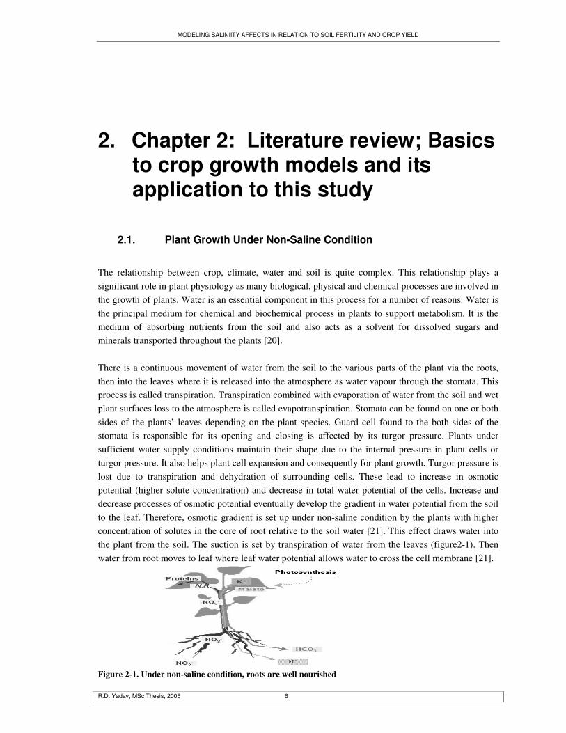
The relationship between crop, climate, water and soil is quite complex. This relationship plays a significant role in plant physiology as many biological, physical and chemical processes are involved in the growth of plants. Water is an essential component in this process for a number of reasons. Water is the principal medium for chemical and biochemical process in plants to support metabolism. It is the medium of absorbing nutrients from the soil and also acts as a solvent for dissolved sugars and minerals transported throughout the plants [20]. There is a continuous movement of water from the soil to the various parts of the plant via the roots, then into the leaves where it is released into the atmosphere as water vapour through the stomata. This process is called transpiration. Transpiration combined with evaporation of water from the soil and wet plant surfaces loss to the atmosphere is called evapotranspiration. Stomata can be found on one or both sides of the plants’ leaves depending on the plant species. Guard cell found to the both sides of the stomata is responsible for its opening and closing is affected by its turgor pressure. Plants under sufficient water supply conditions maintain their shape due to the internal pressure in plant cells or turgor pressure. It also helps plant cell expansion and consequently for plant growth. Turgor pressure is lost due to transpiration and dehydration of surrounding cells. These lead to increase in osmotic potential (higher solute concentration) and decrease in total water potential of the cells. Increase and decrease processes of osmotic potential eventually develop the gradient in water potential from the soil to the leaf. Therefore, osmotic gradient is set up under non-saline condition by the plants with higher concentration of solutes in the core of root relative to the soil water [21]. This effect draws water into the plant from the soil. The suction is set by transpiration of water from the leaves (figure2-1). Then water from root moves to leaf where leaf water potential allows water to cross the cell membrane [21].
Figure 2-1. Under non-saline condition, roots are well nourished
MODELING SALINIITY AFFECTS IN RELATION TO SOIL FERTILITY AND CROP YIELD
R.D. Yadav, MSc Thesis, 2005 7
2.2. Plant Growth Under Saline Condition
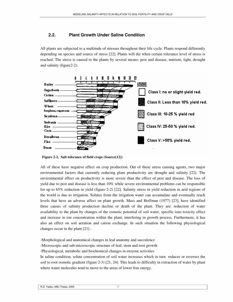
All plants are subjected to a multitude of stresses throughout their life cycle. Plants respond differently depending on species and source of stress [22]. Plants will die when certain tolerance level of stress is reached. The stress is caused to the plants by several means: pest and disease, nutrient, light, drought and salinity (figure2-2).
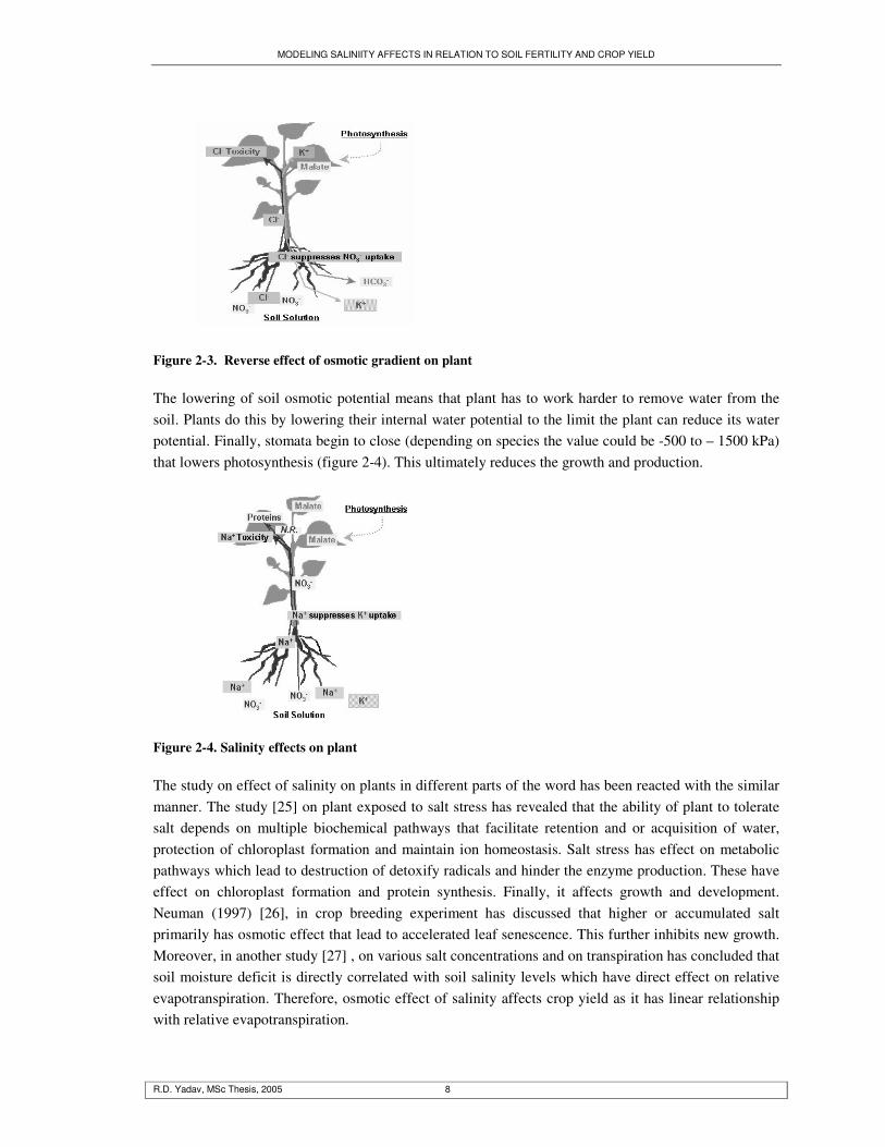
Figure 2-2. Salt tolerance of field crops (Source[12]) All of these have negative effect on crop production. Out of these stress causing agents, two major environmental factors that currently reducing plant productivity are drought and salinity [22]. The environmental effect on productivity is more severe than the effect of pest and disease. The loss of yield due to pest and disease is less than 10% while severe environmental problems can be responsible for up to 65% reduction in yield (figure 2-2) [22]. Salinity stress in yield reduction in arid regions of the world is due to irrigation. Solutes from the irrigation water can accumulate and eventually reach levels that have an adverse affect on plant growth. Mass and Hoffman (1977) [23], have identified three causes of salinity production decline or death of the plant. They are: reduction of water availability to the plant by changes of the osmotic potential of soil water, specific ions toxicity effect and increase in ion concentration within the plant, interfering in growth process. Furthermore, it has also an effect on soil aeration and cation exchange. In such situation the following physiological changes occur in the plant [21] : -Morphological and anatomical changes in leaf anatomy and succulence -Microscopic and sub-microscopic structure of leaf, stem and root growth -Physiological, metabolic and biochemical changes in enzyme activities In saline condition, solute concentration of soil water increases which in turn reduces or reverses the soil to root osmotic gradient (figure 2-3) [21, 24]. This leads to difficulty in extraction of water by plant where water molecules tend to move to the areas of lower free energy.
MODELING SALINIITY AFFECTS IN RELATION TO SOIL FERTILITY AND CROP YIELD
R.D. Yadav, MSc Thesis, 2005 8
Figure 2-3. Reverse effect of osmotic gradient on plant The lowering of soil osmotic potential means that plant has to work harder to remove water from the soil. Plants do this by lowering their internal water potential to the limit the plant can reduce its water potential. Finally, stomata begin to close (depending on species the value could be -500 to – 1500 kPa) that lowers photosynthesis (figure 2-4). This ultimately reduces the growth and production.
Figure 2-4. Salinity effects on plant The study on effect of salinity on plants in different parts of the word has been reacted with the similar manner. The study [25] on plant exposed to salt stress has revealed that the ability of plant to tolerate salt depends on multiple biochemical pathways that facilitate retention and or acquisition of water, protection of chloroplast formation and maintain ion homeostasis. Salt stress has effect on metabolic pathways which lead to destruction of detoxify radicals and hinder the enzyme production. These have effect on chloroplast formation and protein synthesis. Finally, it affects growth and development. Neuman (1997) [26], in crop breeding experiment has discussed that higher or accumulated salt primarily has osmotic effect that lead to accelerated leaf senescence. This further inhibits new growth. Moreover, in another study [27] , on various salt concentrations and on transpiration has concluded that soil moisture deficit is directly correlated with soil salinity levels which have direct effect on relative evapotranspiration. Therefore, osmotic effect of salinity affects crop yield as it has linear relationship with relative evapotranspiration.

MODELING SALINIITY AFFECTS IN RELATION TO SOIL FERTILITY AND CROP YIELD
R.D. Yadav, MSc Thesis, 2005 9
2.3. Crop Simulation Model
Crop simulation models [28, 29], are mathematical representations of plant growth process. These processes are dependent on crop genotype, environment and management. Crop growth models are described by various authors/researchers [30-32]. These models are WOFOST, PS123, EPIC and CROPWAT. WOFOST can predict yield of annual crop on the basis of climate and soil data. It has facility to calculate water limited and nutrient limited crop yield. EPIC model can be used to estimate soil productivity under different degrees of erosion. Similarly, CROPWAT model is used for calculation of water and irrigation requirements on a monthly basis from weather, soil and crop data. These models have played an important role as an indispensable tool for supporting scientific research, crop management and policy analysis [28, 29]. However, these models do not have facility to simulate solute movement (especially salinity). All these facility along with salinity are available in CropSyst (Cropping System Simulation model) and have been tested in many countries under different climatic conditions [28]. According to Stockle et al.[28], CropSyst is a users friendly, multi-year, multi-crop, daily time step cropping systems simulation model developed to serve as an analytical tool to study the effect of climate, soils, and management on cropping systems, productivity and the environment. It has a facility to link to GIS software, a weather generator. The model is also used to simulate the soil water and nitrogen budgets, crop growth and development, crop yield, crop phenology, canopy and root growth, biomass production, residue production and decomposition, soil erosion by water, and salinity. However, these simulation processes are affected by the parameters such as weather, soil characteristics, crop characteristics and crop management these include crop rotation, cultivar selection, irrigation, nitrogen fertilization, soil and irrigation water salinity, tillage operation and residue management.
2.4. Components of CropSyst
2.4.1. Cropsyst Parameter Editor
It is the main user interface which allows users to edit and modify the model parameters, running the model and viewing the output [28]. It has button facility that allows the users to select various components and utilities from menus and tool bar.
2.4.2. Cropping System Simulator
This is the core of the suit of the programme. It contains all the necessary objects, functions for the simulation of crop productivity and crop rotation according to weather, soil and management of an area [28]. The model simulates a single land block fragments having biophysically homogeneous unit area with uniform management and simulation for the land block fragments are created by preparing parameter files describing climate, soil, crop and crop management[28].

MODELING SALINIITY AFFECTS IN RELATION TO SOIL FERTILITY AND CROP YIELD
R.D. Yadav, MSc Thesis, 2005 10
2.4.3. Climate Generator
Climate generator is the weather generators, which predicts precipitation, daily maximum and minimum temperature, solar radiation budget, atmospheric humidity, and speed of wind. All these parameters are used to calculate evapotranspiration (ET).The ET methods available in the CropSyst are simple ET calculation, Priestley-Taylor and Penman-Monteith. One these methods can be used depending on the available climatic data. Simple ET is used if climatic data consist of daily precipitation, maximum and minimum temperature. Priestley-Taylor method is used if the climatic data have daily precipitation, maximum and minimum temperature, and solar radiation. The third most sophisticated method Penman-Monteith ET method which is used with the climatic data is having daily precipitation, daily maximum and minimum temperature, daily solar radiation, daily maximum and minimum relative humidity and daily wind speed. “ClimGen” generated climatic data would be more reliable with complete data required for the generation. It requires 25 years of data on precipitation, 10 years of temperature, and 730 days of wind speed, 730 days of relative humidity or dew point temperature and 5 years data of solar radiation to generate or 730 days data to estimate solar radiation. It also has facility to generate climatic data from monthly climatic data on monthly precipitation, monthly maximum and minimum temperature.
2.4.4. ArcCS
ArcCS is the simulator environment extension programme of cropsyst which facilitates GIS-based spatially oriented simulation capabilities to the cropsyst. Arc cropsyst cooperator is designed to work with database file generated by Arc view or Arc/Info software [28, 33]. Polygon attribute table produced by GIS software is used in ArcCS to identify, generate and run a simulation scenario for each unique land block fragment. A new polygon attribute table of CropSyst output variables is generated, which can be used by Arc/Info or Arc view in order to produce CropSyst outputs maps [28, 33]. Moreover, statistical analysis such as mean, coefficient of variance and cumulative probability distribution of annual and harvested outputs of variables are used for generating maps.
2.5. Sub-Model Description
2.5.1. Water Budget
Water budget of the cropsyst includes precipitation, irrigation, runoff, interception, infiltration, soil water redistribution in the profile, deep percolation, crop transpiration and evaporation. The model is based on simple cascade system of water redistribution in the soil profile and it has option of a numerical solution of the Richard's soil flow equation of Campbell and Ross and Bristow as well [28, 33]. “ClimGen” of the model allows users to estimate daily solar radiation and humidity from temperature, daily wind data provided at least for two years of complete daily records. This is used to compute potential evapotranspiration (ET) by multiplying with crop coefficient. Partitioning of potential crop transpiration and potential soil evaporation is determined by crop ground coverage and actual

MODELING SALINIITY AFFECTS IN RELATION TO SOIL FERTILITY AND CROP YIELD
R.D. Yadav, MSc Thesis, 2005 11
transpiration and soil evaporation, depends on water availability in the soil profile explored by roots and soil surface respectively [28, 33].
2.5.2. Nitrogen Budget
Nitrogen transformations, ammonium sorption, symbiotic nitrogen fixation, crop nitrogen demand and crop nitrogen uptake are the process used separately for nitrate nitrogen and ammonical nitrogen budget in cropsyst presented by Stockle and Campbell [34] and symbiotic nitrogen is based on Bouniols[28, 33]. Stockle et al [28, 33] had adopted the crop nitrogen uptake in the model of approach presented by Godwins and Jones in 1991[33] where, N uptake is determined as the minimum of crop nitrogen demand and potential nitrogen uptake with following equation: ND = (NCmax - NCONCb) * (TM + RM) + NCmax * (RGpot + Gpot) Where, ND (kg/ha) is the crop nitrogen demand. NCmax (kg N/kg biomass) is the crop maximum nitrogen concentration. NCONCb (kg N/kg biomass) is crop nitrogen concentration before new growth. TM (kg/ha) is the cumulative above ground crop biomass. RM (kg/ha) is the cumulative root biomass. RGpot (kg/ha) is the potential new root growth. Gpot (kg/ha) is the potential new top growth. The demand of nitrogen of the crop is the amount of nitrogen required for the growth plus the deficiency demand. It is the difference between the crop maximum and actual nitrogen concentration. Water budget interacts with chemical budget such as nitrogen, salinity and other solute to produce simulation of transport of these chemicals within the soil [28, 33]. All of these balances are checked during the simulation and errors are reported.
2.5.3. Crop Phenology
Thermal time is the required daily accumulation of average air temperature above a base temperature and below a cutoff temperature to reach given growth stages. It is computed by following equation[33]: GD day = Tavg - TGDdaybase CGDday = CGDday-1 + GDday
Where, GDday (°C-days) = Today's thermal time. CGDday (°C-days) = Today's accumulated thermal time since planting.
MODELING SALINIITY AFFECTS IN RELATION TO SOIL FERTILITY AND CROP YIELD
R.D. Yadav, MSc Thesis, 2005 12
TGD = Daybase temperature Tcutoff = Crop input parameters that define the range of temperatures for viable development. Tmin (°C) = The daily minimum air temperature. Tmax (°C) = The daily maximum air temperature. Tavg = The daily average air temperature. Thermal time is used for the simulation of crop development in this model and its accumulation could be accelerated by water stress based on the concept of increased of crop temperature[28, 33]. Jackson, in 1982 has explained in his infrared thermometry literature that crop temperature for stressed and unstressed crops is the function of the vapour pressure deficit of the atmosphere[28, 33].
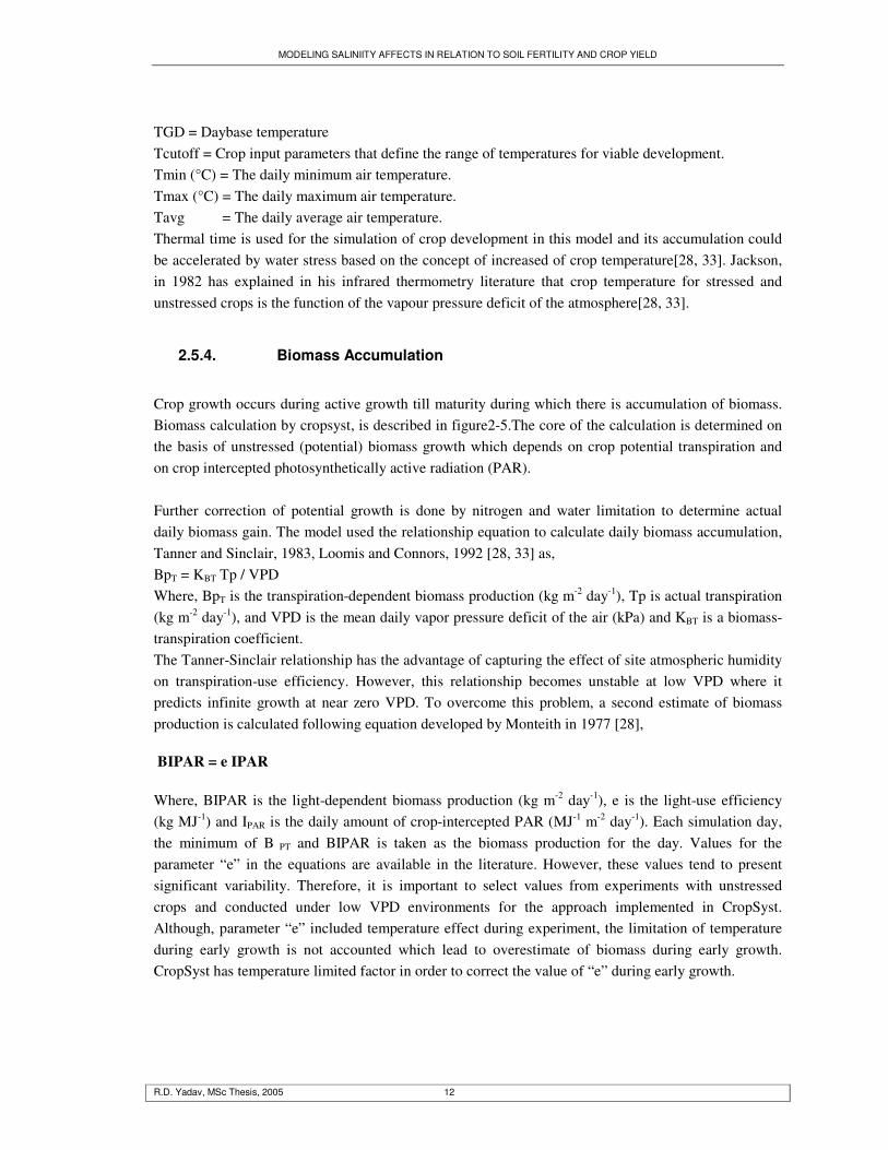
2.5.4. Biomass Accumulation
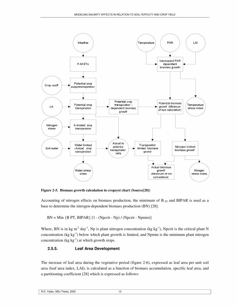
Crop growth occurs during active growth till maturity during which there is accumulation of biomass. Biomass calculation by cropsyst, is described in figure2-5.The core of the calculation is determined on the basis of unstressed (potential) biomass growth which depends on crop potential transpiration and on crop intercepted photosynthetically active radiation (PAR). Further correction of potential growth is done by nitrogen and water limitation to determine actual daily biomass gain. The model used the relationship equation to calculate daily biomass accumulation, Tanner and Sinclair, 1983, Loomis and Connors, 1992 [28, 33] as, BpT = KBT Tp / VPD Where, BpT is the transpiration-dependent biomass production (kg m-2 day-1), Tp is actual transpiration (kg m-2 day-1), and VPD is the mean daily vapor pressure deficit of the air (kPa) and KBT is a biomass-transpiration coefficient. The Tanner-Sinclair relationship has the advantage of capturing the effect of site atmospheric humidity on transpiration-use efficiency. However, this relationship becomes unstable at low VPD where it predicts infinite growth at near zero VPD. To overcome this problem, a second estimate of biomass production is calculated following equation developed by Monteith in 1977 [28], BIPAR = e IPAR Where, BIPAR is the light-dependent biomass production (kg m-2 day-1), e is the light-use efficiency (kg MJ-1) and IPAR is the daily amount of crop-intercepted PAR (MJ-1 m-2 day-1). Each simulation day, the minimum of B PT and BIPAR is taken as the biomass production for the day. Values for the parameter “e” in the equations are available in the literature. However, these values tend to present significant variability. Therefore, it is important to select values from experiments with unstressed crops and conducted under low VPD environments for the approach implemented in CropSyst. Although, parameter “e” included temperature effect during experiment, the limitation of temperature during early growth is not accounted which lead to overestimate of biomass during early growth. CropSyst has temperature limited factor in order to correct the value of “e” during early growth.
MODELING SALINIITY AFFECTS IN RELATION TO SOIL FERTILITY AND CROP YIELD
R.D. Yadav, MSc Thesis, 2005 13
Figure 2-5. Biomass growth calculation in cropsyst chart (Source[28]) Accounting of nitrogen effects on biomass production, the minimum of B PT and BIPAR is used as a base to determine the nitrogen-dependent biomass production (BN) [28]: BN = Min {B PT, BIPAR} [1 - (Npcrit - Np) / (Npcrit - Npmin)] Where, BN is in kg m-2 day-1, Np is plant nitrogen concentration (kg kg-1), Npcrit is the critical plant N concentration (kg kg-1) below which plant growth is limited, and Npmin is the minimum plant nitrogen concentration (kg kg-1) at which growth stops.
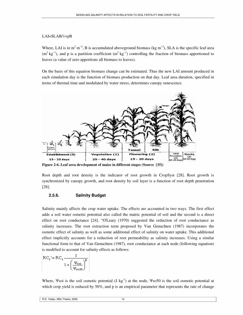
2.5.5. Leaf Area Development
The increase of leaf area during the vegetative period (figure 2-6), expressed as leaf area per unit soil area (leaf area index, LAI), is calculated as a function of biomass accumulation, specific leaf area, and a partitioning coefficient [28] which is expressed as follows:
MODELING SALINIITY AFFECTS IN RELATION TO SOIL FERTILITY AND CROP YIELD
R.D. Yadav, MSc Thesis, 2005 14
LAI=SLAB/1+pB Where, LAI is in m2 m−2, B is accumulated aboveground biomass (kg m−2), SLA is the specific leaf area (m2 kg−1), and p is a partition coefficient (m2 kg−1) controlling the fraction of biomass apportioned to leaves (a value of zero apportions all biomass to leaves). On the basis of this equation biomass change can be estimated. Thus the new LAI amount produced in each simulation day is the function of biomass production on that day. Leaf area duration, specified in terms of thermal time and modulated by water stress, determines canopy senescence.
Figure 2-6. Leaf area development of maize in different stages (Source [35]) Root depth and root density is the indicator of root growth in CropSyst [28]. Root growth is synchronized by canopy growth, and root density by soil layer is a function of root depth penetration [28].
2.5.6. Salinity Budget
Salinity mainly affects the crop water uptake. The effects are accounted in two ways. The first effect adds a soil water osmotic potential also called the matric potential of soil and the second is a direct effect on root conductance [24]. “O'Leary (1970) suggested the reduction of root conductance as salinity increases. The root extraction term proposed by Van Genuchten (1987) incorporates the osmotic effect of salinity as well as some additional effect of salinity on water uptake. This additional effect implicitly accounts for a reduction of root permeability as salinity increases. Using a similar functional form to that of Van Genuchten (1987), root conductance at each node (following equation) is modified to account for salinity effects as follows:
Where, �soi is the soil osmotic potential (J kg-1) at the node, �so50 is the soil osmotic potential at which crop yield is reduced by 50%, and p is an empirical parameter that represents the rate of change

MODELING SALINIITY AFFECTS IN RELATION TO SOIL FERTILITY AND CROP YIELD
R.D. Yadav, MSc Thesis, 2005 15
of the salinity response. Both the osmotic potential and the osmotic potential at 50% reduction are expressed in a saturation extract base”[24]. The long term result of lysimeter experiment of soil salinity, soil type and crop variety by Katerji et al [36] revealed that salinity affected the pre-dawn leaf water potential, stomatal conductance, evapotranspiration, leaf area and yield. The following sub model flow diagram (figure 2-7) describes the simulation of salinity by using some parameters from soil, management, and weather files, which in turn results in the simulation of crop growth and yield.
Figure 2-7. Sub model of salinity simulation
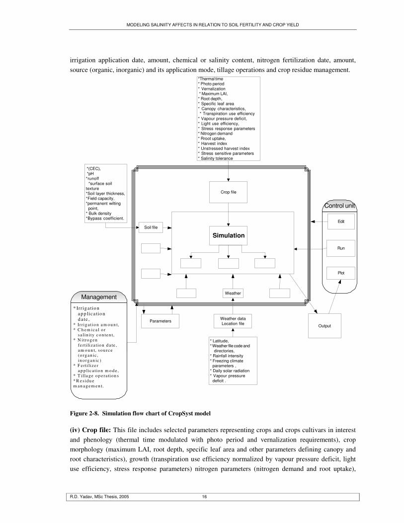
2.6. Data Requirements
Location, soil, crop, and management files are the four input data files, as described below, required to run this model [37]. However, simulation control file combines the inputs file as desired to produce specific simulation run. Separation of files allows for an easier link of CropSyst simulations with GIS as shown in figure 2-8. (i) Location file: It includes information such as latitude, weather file code and directories, rainfall intensity (for erosion), freezing climate parameters (where soil freeze), local parameters to generate daily solar radiation and vapor pressure deficit values. (ii) Soil file: It includes cation exchange capacity (CEC), pH (For ammonia volatilization), runoff calculation parameters, surface soil texture and five soil parameters such as layer thickness, field capacity, permanent wilting point, bulk density and bypass coefficient. (iii) Management file: It includes automatic events for optimum management for maximum growth such as irrigation and nitrogen fertilization. Under schedule management events information such as
MODELING SALINIITY AFFECTS IN RELATION TO SOIL FERTILITY AND CROP YIELD
R.D. Yadav, MSc Thesis, 2005 16
irrigation application date, amount, chemical or salinity content, nitrogen fertilization date, amount, source (organic, inorganic) and its application mode, tillage operations and crop residue management.
Weather dataLocation file
Soil file
Crop file
Output
Simulation
Parameters
Weather
Edit
Run
Plot
Control unit
*(CEC), *pH*runoff *surface soiltexture*Soil layer thickness,*Field capacity,*permanent wilting point,* Bulk density*Bypass coefficient.
* Latitude,* Weather file code and directories,* Rainfall intensity* Freezing climate parameters ,* Daily solar radiation* Vapour pressure deficit .
*Thermal time* Photo period* Vernalization * Maximum LAI,* Root depth,* Specific leaf area* Canopy characteristics, * Transpiration use efficiency* Vapour pressure deficit,* Light use efficiency,* Stress response parameters* Nitrogen demand* Rroot uptake,* Harvest index* Unstressed harvest index* Stress sensitive parameters* Salinity tolerance
Management
* Irrig a tio n ap p lica tio n d a te ,
* Ir riga tio n a m o u n t, * C h em ica l o r
sa lin ity c o n ten t, * N itro g en
fe rtiliza tio n d a te , am o u n t, so u rce (o rg an ic , in o rgan ic )
* F e rtilize r ap p lic atio n m o d e ,
* T illa ge o p e ra tion s * R e sidu e m an ag e m en t.
Figure 2-8. Simulation flow chart of CropSyst model
(iv) Crop file: This file includes selected parameters representing crops and crops cultivars in interest and phenology (thermal time modulated with photo period and vernalization requirements), crop morphology (maximum LAI, root depth, specific leaf area and other parameters defining canopy and root characteristics), growth (transpiration use efficiency normalized by vapour pressure deficit, light use efficiency, stress response parameters) nitrogen parameters (nitrogen demand and root uptake),
MODELING SALINIITY AFFECTS IN RELATION TO SOIL FERTILITY AND CROP YIELD
R.D. Yadav, MSc Thesis, 2005 17
harvest index (unstressed harvest index and stress sensitive parameters) and salinity tolerance are the information needed under this input file.
2.7. Crop Growth Simulation Model PS 123
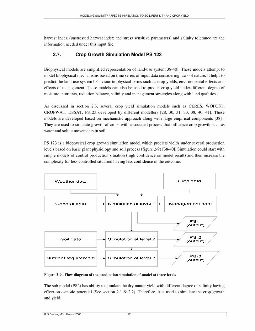
Biophysical models are simplified representation of land-use system[38-40]. These models attempt to model biophysical mechanisms based on time series of input data considering laws of nature. It helps to predict the land-use system behaviour in physical terms such as crop yields, environmental effects and effects of management. These models can also be used to predict crop yield under different degree of moisture, nutrients, radiation balance, salinity and management strategies along with land qualities. As discussed in section 2.3, several crop yield simulation models such as CERES, WOFOST, CROPWAT, DSSAT, PS123 developed by different modellers [28, 30, 31, 33, 38, 40, 41]. These models are developed based on mechanistic approach along with large empirical components [38] . They are used to simulate growth of crops with associated process that influence crop growth such as water and solute movements in soil. PS 123 is a biophysical crop growth simulation model which predicts yields under several production levels based on basic plant physiology and soil process (figure 2-9) [38-40]. Simulation could start with simple models of control production situation (high confidence on model result) and then increase the complexity for less controlled situation having less confidence in the outcome.
Figure 2-9. Flow diagram of the production simulation of model at three levels The sub model (PS2) has ability to simulate the dry matter yield with different degree of salinity having effect on osmotic potential (See section 2.1 & 2.2). Therefore, it is used to simulate the crop growth and yield.
MODELING SALINIITY AFFECTS IN RELATION TO SOIL FERTILITY AND CROP YIELD
R.D. Yadav, MSc Thesis, 2005 18
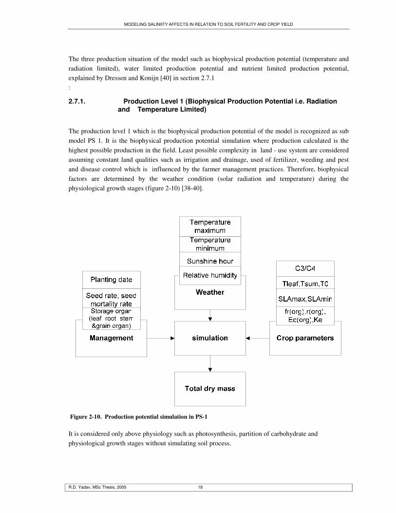
The three production situation of the model such as biophysical production potential (temperature and radiation limited), water limited production potential and nutrient limited production potential, explained by Dressen and Konijn [40] in section 2.7.1 :
2.7.1. Production Level 1 (Biophysical Production Potential i.e. Radiation and Temperature Limited)
The production level 1 which is the biophysical production potential of the model is recognized as sub model PS 1. It is the biophysical production potential simulation where production calculated is the highest possible production in the field. Least possible complexity in land - use system are considered assuming constant land qualities such as irrigation and drainage, used of fertilizer, weeding and pest and disease control which is influenced by the farmer management practices. Therefore, biophysical factors are determined by the weather condition (solar radiation and temperature) during the physiological growth stages (figure 2-10) [38-40].
Figure 2-10. Production potential simulation in PS-1 It is considered only above physiology such as photosynthesis, partition of carbohydrate and physiological growth stages without simulating soil process.
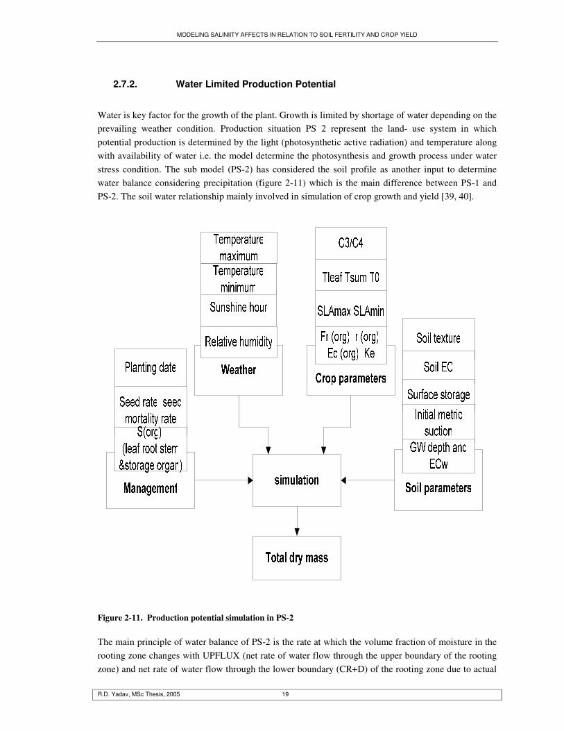
MODELING SALINIITY AFFECTS IN RELATION TO SOIL FERTILITY AND CROP YIELD
R.D. Yadav, MSc Thesis, 2005 19
2.7.2. Water Limited Production Potential
Water is key factor for the growth of the plant. Growth is limited by shortage of water depending on the prevailing weather condition. Production situation PS 2 represent the land- use system in which potential production is determined by the light (photosynthetic active radiation) and temperature along with availability of water i.e. the model determine the photosynthesis and growth process under water stress condition. The sub model (PS-2) has considered the soil profile as another input to determine water balance considering precipitation (figure 2-11) which is the main difference between PS-1 and PS-2. The soil water relationship mainly involved in simulation of crop growth and yield [39, 40].
Figure 2-11. Production potential simulation in PS-2 The main principle of water balance of PS-2 is the rate at which the volume fraction of moisture in the rooting zone changes with UPFLUX (net rate of water flow through the upper boundary of the rooting zone) and net rate of water flow through the lower boundary (CR+D) of the rooting zone due to actual
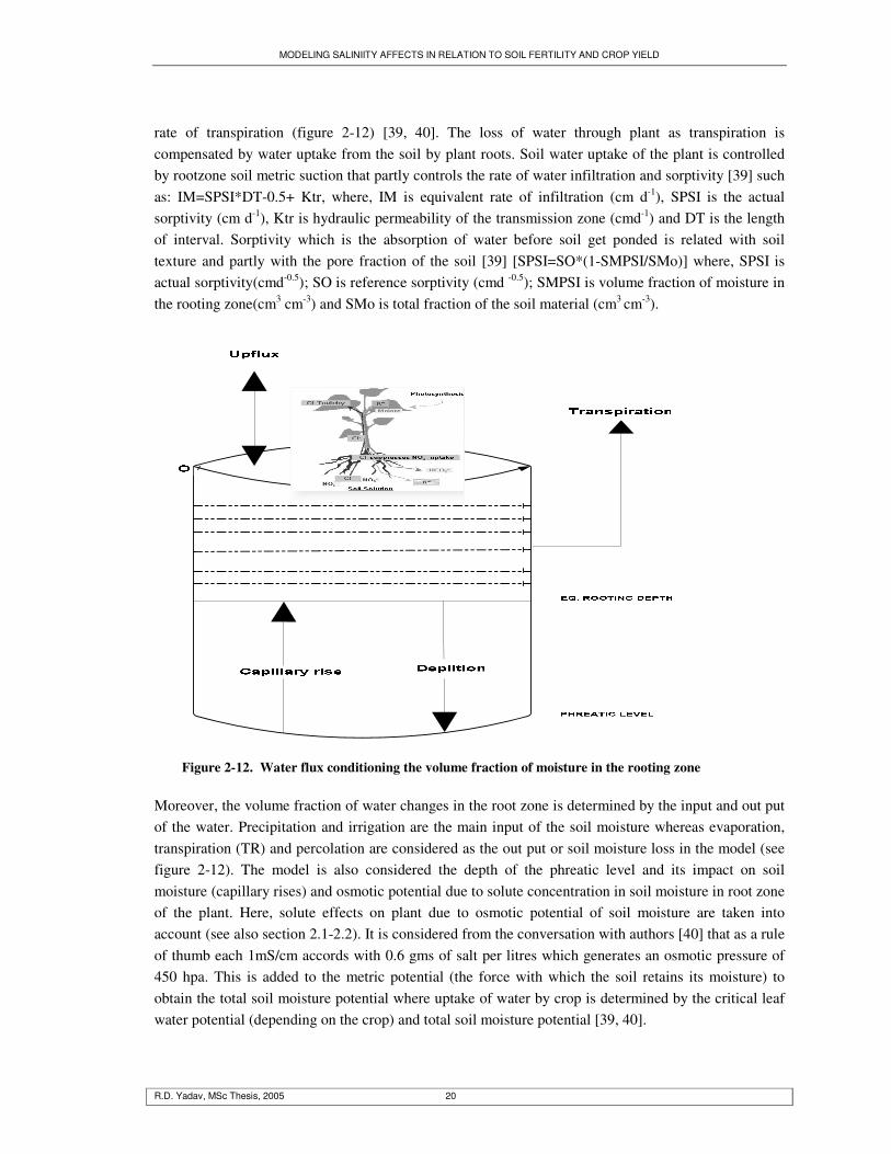
MODELING SALINIITY AFFECTS IN RELATION TO SOIL FERTILITY AND CROP YIELD
R.D. Yadav, MSc Thesis, 2005 20
rate of transpiration (figure 2-12) [39, 40]. The loss of water through plant as transpiration is compensated by water uptake from the soil by plant roots. Soil water uptake of the plant is controlled by rootzone soil metric suction that partly controls the rate of water infiltration and sorptivity [39] such as: IM=SPSI*DT-0.5+ Ktr, where, IM is equivalent rate of infiltration (cm d-1), SPSI is the actual sorptivity (cm d-1), Ktr is hydraulic permeability of the transmission zone (cmd-1) and DT is the length of interval. Sorptivity which is the absorption of water before soil get ponded is related with soil texture and partly with the pore fraction of the soil [39] [SPSI=SO*(1-SMPSI/SMo)] where, SPSI is actual sorptivity(cmd-0.5); SO is reference sorptivity (cmd -0.5); SMPSI is volume fraction of moisture in the rooting zone(cm3 cm-3) and SMo is total fraction of the soil material (cm3 cm-3).
Figure 2-12. Water flux conditioning the volume fraction of moisture in the rooting zone Moreover, the volume fraction of water changes in the root zone is determined by the input and out put of the water. Precipitation and irrigation are the main input of the soil moisture whereas evaporation, transpiration (TR) and percolation are considered as the out put or soil moisture loss in the model (see figure 2-12). The model is also considered the depth of the phreatic level and its impact on soil moisture (capillary rises) and osmotic potential due to solute concentration in soil moisture in root zone of the plant. Here, solute effects on plant due to osmotic potential of soil moisture are taken into account (see also section 2.1-2.2). It is considered from the conversation with authors [40] that as a rule of thumb each 1mS/cm accords with 0.6 gms of salt per litres which generates an osmotic pressure of 450 hpa. This is added to the metric potential (the force with which the soil retains its moisture) to obtain the total soil moisture potential where uptake of water by crop is determined by the critical leaf water potential (depending on the crop) and total soil moisture potential [39, 40].
MODELING SALINIITY AFFECTS IN RELATION TO SOIL FERTILITY AND CROP YIELD
R.D. Yadav, MSc Thesis, 2005 21
CLIM.DAT, CROP.DAT and SOIL.DAT are three main input files considered in sub model PS2. The SOIL.DAT files which is the inputs not considered in PS1, consists soil parameters in the following five lines[39, 40]: Line # 1 “SOILLABLES” Line # 2 SMo (cm3 cm-3), GAM (cm-2) Line # 3 PSImax(cm), Ko (cm d-1), ALFA (cm-1), AK (cm-2.4 d-1) Line # 4 SO (cm day-0.5), Ktr (cm d-1) Line # 5 dummy value Where, SMo is total pore space GAM is geometry factor PSImax is temperature specific suction boundary; Ko is saturated hydraulic conductivity; ALFA is texture specific geometry constant (low suction parameter) AK is texture specific empirical constant (high suction parameter) SO is standard sorptivity and Ktr is hydraulic permeability of the transmission zone. The hydraulic conductivity of the soil which is the function of metric suction and geometry is calculated by SOIL.DAT file in sub model PS 2. Soil peds and pores (voids) determine the soil geometry. The hydraulic conductivity matric suction and relative hydraulic conductivity suctions are texture specific of the field [39, 40]. This relationship is explained as: If PSI � PSImax then KPSI = Ko* exp (-ALFA*PSI) else KPSI = AK*PSI-n Once the texture is selected, the programme uses the proper indicative value of texture class available in SOIL.DAT file.
2.7.3. Production Level 3: Assessing Fertilizer Requirements (Nitrogen Limited)
Growth of the plants is determined by shortage of water, weather and nitrogen (N). Nitrogen is the key plant essential element which has significant effects over vegetative growth of the plant. Moreover, rapid transformation of nitrogen makes it more limiting nutrients than other nutrients. This is common in rainfed condition where recommended dose of nutrients applied with organic manures. The model at production level 3 gives nutrient balance based on input out put calculation. Scores of nutrients (Macro and micro) required to complete the growth cycle of the plant. Production potential examines availability of nutrient to the crop. This is determined by the supply of nutrients to the rooting zone through various means (mineralization, atmospheric deposition and fixation, manure applied), losses from the rooting zone (leaching, volatilization, erosion and plant uptake), inactivation of nutrient elements (low solubility compound,) and their various interactions (synergisms, antagonisms)[40]. Modelling yield in terms of supply of nutrients is complex and dynamic which depends on temperature, photosynthetically active radiation, availability of water and availability of nutrients. Nitrogen is the main nutrient to take part in growth of plants. Soil is open system for nitrogen
MODELING SALINIITY AFFECTS IN RELATION TO SOIL FERTILITY AND CROP YIELD
R.D. Yadav, MSc Thesis, 2005 22
fertilizer. Plant needs this nutrient through out the growing season. Therefore, nitrogen modelling could be come up with satisfactory result in prediction of crop yield. PS-3 is basically performed best in one element in short supply.
2.8. Applying the Model to Track Down Salt Movement
Crop yield depends on many factors such as climate, soil, crop, and management. Therefore, a suitable method for precise result covering all these factors need to be applied. CropSyst is the model that considers solute movement on all the stages of growth in yield assessment. Therefore, this method could be applied for yield assessment in relation to salinity. It is also used to simulate the soil water and nitrogen budgets, crop growth and development, crop yield, residue production and decomposition, soil erosion by water, and salinity. Moreover, input files manipulation, verify parameters for errors and cross compatibility, create and execute simulations, produce text, graphics and link to the spreadsheet are the other advantages to the users. The model has been applied on several agricultural practices assessment successfully under different climatic condition in different part of the world [24, 28, 42]. It was applied to evaluate two levels of nitrogen fertilization on seven rotations implemented on a variety of soils in the Po Valley, Italy for estimation of drainage and nitrogen leaching in different soil–weather–management scenarios [37]. An assessment of the adaptation of improved cultivars of millet in Burkina Faso was conducted by applying this model [43].The model considers the solute movement affecting crop growth, development and yield. Therefore, it is applied in this study. Now a days, the development of GIS and remote sensing based models are used in various fields of studies. The GIS and remote sensing tools and techniques are commonly applied in natural resources management. These tools and techniques are also felt to apply in this study in order to compare the results obtained from the mechanistic models. The followings are the GIS and remote sensing models felt to be used in this research.
2.8.1. Geo-statistics in Spatial Modelling
Soil properties vary irregularly in the real world and require appropriate estimation approach for unsampled points [44]. Geostatistic interpolation technique, such as kriging, have been used for estimation of soil properties at unsampled points and also in the other field of study [44, 45]. Different Kriging interpolation techniques were applied and results were compared to come up with salinity and soil fertility map. Post plot of the data can be generated using ILWIS software in order to visualize spatial nature of data. It guides to observe the relation between the points. Lag distance plays an important role in variogram model selection where too large lag distance masks the spatial whereas small lag distance does not capture sufficient samples [46, 47]. Actual lag distance has to be chosen for further analysis. The next step is to generate spatial correlation with best lag distance. It gives an idea about the number of point pair that lies in the selected lag distance and how semi-variance increases with increasing lag distance.

MODELING SALINIITY AFFECTS IN RELATION TO SOIL FERTILITY AND CROP YIELD
R.D. Yadav, MSc Thesis, 2005 23
Once spatial auto- correlation analysis is done the following steps have to be performed in Kriging (ordinary kriging, kriging with external drift, and indicator kriging) interpolation operation: -Estimation of variogram -Estimation of parameters of the variogram model -Estimation of the surface (= map) using point interpolation (Kriging) Graphically, semivariogram and lag distance are being represented. This shows the nature of spatial relationship or how semivarience varied with lag distances and guides in selection of variogram model. There are several variogram models used in different studies. Spherical and exponential variogram model have been commonly used in soil studies as values in small separation distances show linear relation which is lost at larger distances [47]. Therefore, these models with the estimated parameters such as sill, range, and nugget could be applied for estimation of salinity and fertility of soil surface. Moreover, indicator kriging would also be carried out by applying crops threshold salinity values in order to generate salinity hot spot map.
2.8.2. Modelling Land Evaluation Using Spatial Multiple Criteria Evaluation (SMCE)
a. Introduction to SMCE Scores of factors have to be considered in the development and planning in decision making for land evaluation and management processes. Remote sensing and GIS technology offer great potential to capture data from variety of earth observation platforms and incorporate them in a spatial manner [48-50]. GIS is an appropriate technology for data extraction and storage, data management, manipulation, and visualization [48]. The only setback is that GIS lack analytical capabilities in order to support management and decision making [48, 49]. However in decision making process it is required to integrate variety of information from different sources with tools and techniques in GIS such as SMCE which is combination of multi-criteria evaluation methods and spatial analyses [48, 49]. It is a process that combines and transforms geographical data (the input) into land suitability class (the output). Multidimensional geographical data and information can be aggregated into one-dimensional values for the land suitability in this process [48, 49]. Several layers of criteria as groups and sub groups is used in the decision making process. This process involves not only utilization of geographical data, but also the user’s judgment and the manipulation of data and preferences based on specified judgment rules. This rules also known as criteria are based on expert judgment. A criterion is the indication of how well an alternative reaches the objective. Criteria is called spatial when it needs the information of location, which are used to evaluate the alternatives by measuring the impacts [49]. According to Sharifi and Retsios [49], criteria can be represented in the form of digital map stored in GIS database as layers. These layers are the input data for SMCE[49, 50]. Several approaches can be

MODELING SALINIITY AFFECTS IN RELATION TO SOIL FERTILITY AND CROP YIELD
R.D. Yadav, MSc Thesis, 2005 24
used to generate input maps for SMCE where it is capable to accept maps of different domain. Once all criteria maps are made, they are divided between deterministic, probabilistic or possibility maps. SMCE can be implemented if these conditions are met and decision is made on the basis of a set of criteria rules. Finally, the analysis must have alternatives based on modification of decision rules. The method is adopted in this present work to model crop suitability in terms of salinity and soil fertility. b. SMCE design based on problem SMCE is designed to come up with alternative solution of the problems. The followings are the main steps of SMCE to have potential sites for the intended purposes.
• Problem structuring leads to identification of main criteria that could be considered as necessary and preferred. Information related to criteria has to be collected and presented in a proper format.
• Once criteria are collected and presented in the proper format, relevant transformation function has to be identified to convert the criteria into same units referred to as standardisation.
• Then relative position of the criteria has to be identified with respects to others considering their level of contribution in order to achieve related objectives (weight assessment).
• After that suitability assessment is carried out, each pixel is assigned with suitability value.
• Finally potential site is designed by connecting value of suitable pixels.
2.8.3. Possibility of Point Data Transformation to Area Using Remote Sensing
Remote sensing technique is used to collect, detect and interpret spatial variability from distance by mean of sensors. Sensors measure the electromagnetic radiations reflectance of the earth surface features. The radiation energy is transmitted through space in waveform and is defined by wavelength and amplitude or oscillation. The wavelength of electromagnetic spectrum ranges from less than 0.03 nm (Gamma rays) more than 30 cm (radio energy). Wavelength ranges from 0.4 to 1.5 mm commonly used to land resources surveys with remote sensing techniques. Soil salinity caused by natural and human induced process is major environmental hazard [4]. Therefore, careful monitoring of soil salinity status and its variation to curb degradation trend is necessary to secure sustainable land use and management to increase crop yield. A variety of remote sensing data has been used for identifying and monitoring salt-affected areas. The remote sensing data such as aerial photo, video images, and infrared thermography are used in detecting temporal changes of salt related surface features. Similarly airborne geophysics, hyper-spectral sensors and electromagnetic induction meters combine ground data; have shown potential for mapping depth of salinity occurrence [4]. Remote sensing has been used in both qualitative and quantitative aspect. Estimating food supply to monitor famine condition and for the international trade purposes with coarser resolutions satellite imagery are the examples of qualitative use of remote sensing [51]. Spatial and temporal distribution of crop productivity using remote sensing is the quantity use.
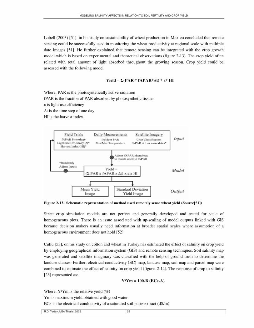
MODELING SALINIITY AFFECTS IN RELATION TO SOIL FERTILITY AND CROP YIELD
R.D. Yadav, MSc Thesis, 2005 25
Lobell (2003) [51], in his study on sustainability of wheat production in Mexico concluded that remote sensing could be successfully used in monitoring the wheat productivity at regional scale with multiple date images [51]. He further explained that remote sensing can be integrated with the crop growth model which is based on experimental and theoretical observations (figure 2-13). The crop yield often related with total amount of light absorbed throughout the growing season. Crop yield could be assessed with the following model
Yield = �(PAR * fAPAR*�t) * �* HI Where, PAR is the photosyntetically active radiation fPAR is the fraction of PAR absorbed by photosynthetic tissues � is light use efficiency �t is the time step of one day HI is the harvest index
Figure 2-13. Schematic representation of method used remotely sense wheat yield (Source[51]) Since crop simulation models are not perfect and generally developed and tested for scale of homogeneous plots. There is an issue associated with up-scaling of model outputs linked with GIS because decision makers usually need information at broader spatial scales where assumption of a homogeneous environment does not hold [52]. Cullu [53], on his study on cotton and wheat in Turkey has estimated the effect of salinity on crop yield by employing geographical information system (GIS) and remote sensing techniques. Soil salinity map was generated and satellite imaginary was classified with the help of ground truth to determine the landuse classes. Further, electrical conductivity (EC) map, landuse map, soil map and parcel map were combined to estimate the effect of salinity on crop yield (figure. 2-14). The response of crop to salinity [23] represented as:
Y/Ym = 100-B (ECe-A) Where, Y/Ym is the relative yield (%) Ym is maximum yield obtained with good water ECe is the electrical conductivity of a saturated soil paste extract (dS/m)
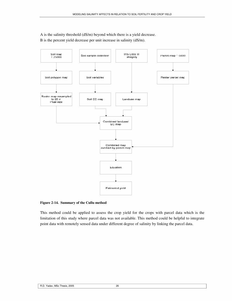
MODELING SALINIITY AFFECTS IN RELATION TO SOIL FERTILITY AND CROP YIELD
R.D. Yadav, MSc Thesis, 2005 26
A is the salinity threshold (dS/m) beyond which there is a yield decrease. B is the percent yield decrease per unit increase in salinity (dS/m).
Figure 2-14. Summary of the Cullu method This method could be applied to assess the crop yield for the crops with parcel data which is the limitation of this study where parcel data was not available. This method could be helpful to integrate point data with remotely sensed data under different degree of salinity by linking the parcel data.
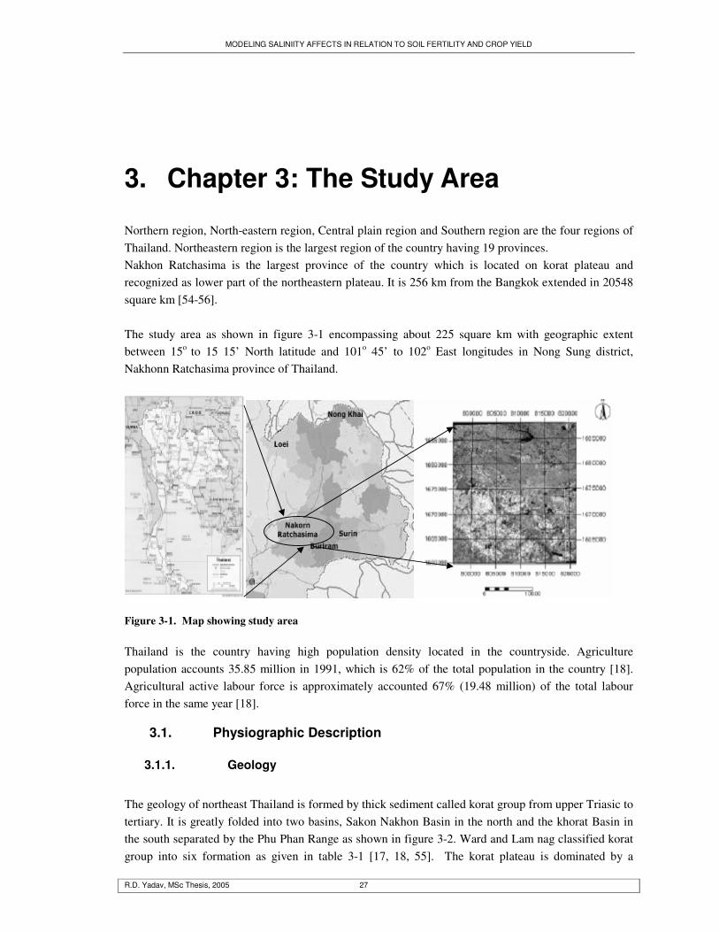
MODELING SALINIITY AFFECTS IN RELATION TO SOIL FERTILITY AND CROP YIELD
R.D. Yadav, MSc Thesis, 2005 27
3. Chapter 3: The Study Area
Northern region, North-eastern region, Central plain region and Southern region are the four regions of Thailand. Northeastern region is the largest region of the country having 19 provinces. Nakhon Ratchasima is the largest province of the country which is located on korat plateau and recognized as lower part of the northeastern plateau. It is 256 km from the Bangkok extended in 20548 square km [54-56]. The study area as shown in figure 3-1 encompassing about 225 square km with geographic extent between 15o to 15 15’ North latitude and 101o 45’ to 102o East longitudes in Nong Sung district, Nakhonn Ratchasima province of Thailand.
Figure 3-1. Map showing study area Thailand is the country having high population density located in the countryside. Agriculture population accounts 35.85 million in 1991, which is 62% of the total population in the country [18]. Agricultural active labour force is approximately accounted 67% (19.48 million) of the total labour force in the same year [18].
3.1. Physiographic Description
3.1.1. Geology
The geology of northeast Thailand is formed by thick sediment called korat group from upper Triasic to tertiary. It is greatly folded into two basins, Sakon Nakhon Basin in the north and the khorat Basin in the south separated by the Phu Phan Range as shown in figure 3-2. Ward and Lam nag classified korat group into six formation as given in table 3-1 [17, 18, 55]. The korat plateau is dominated by a
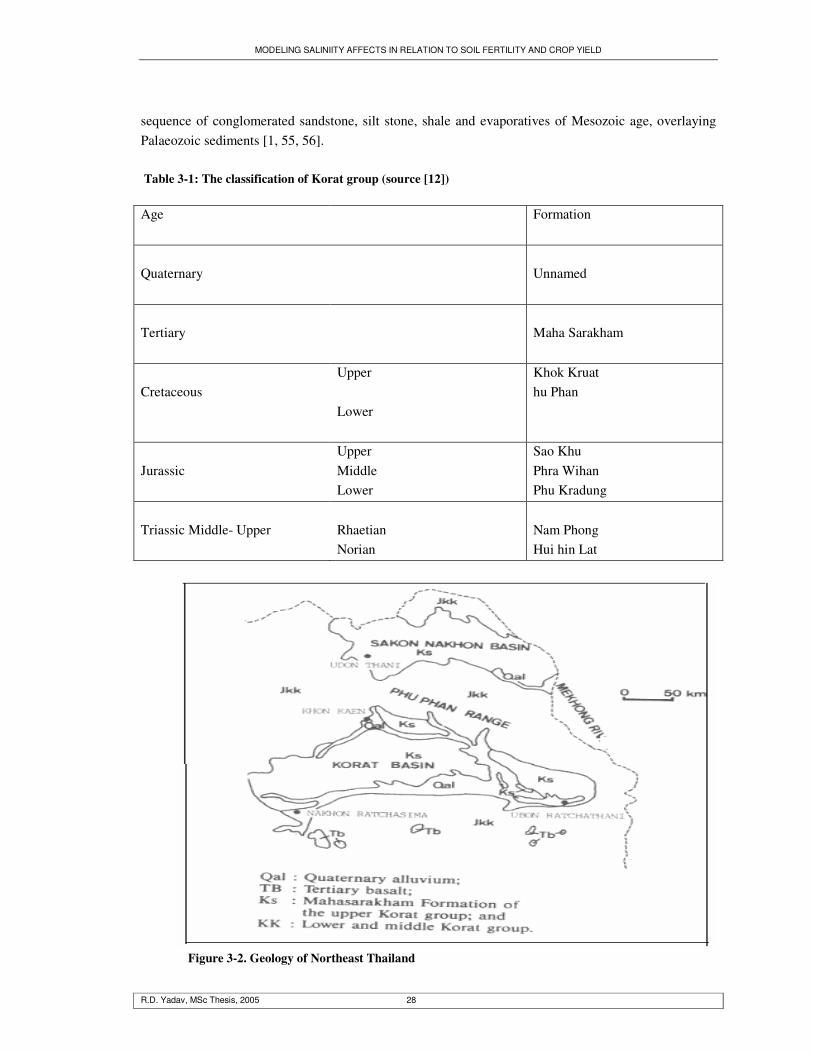
MODELING SALINIITY AFFECTS IN RELATION TO SOIL FERTILITY AND CROP YIELD
R.D. Yadav, MSc Thesis, 2005 28
sequence of conglomerated sandstone, silt stone, shale and evaporatives of Mesozoic age, overlaying Palaeozoic sediments [1, 55, 56]. Table 3-1: The classification of Korat group (source [12]) Age
Formation
Quaternary
Unnamed
Tertiary
Maha Sarakham
Cretaceous
Upper Lower
Khok Kruat hu Phan
Jurassic
Upper Middle Lower
Sao Khu Phra Wihan Phu Kradung
Triassic Middle- Upper
Rhaetian Norian
Nam Phong Hui hin Lat
Figure 3-2. Geology of Northeast Thailand

MODELING SALINIITY AFFECTS IN RELATION TO SOIL FERTILITY AND CROP YIELD
R.D. Yadav, MSc Thesis, 2005 29
3.1.2. Geomorphology
According to Wada et al [54], korat plateau which is in the shape of a square is found in the northeast Thailand. It is boarded to the north and east by the Mekhong river, Phetchabun mountain range in the west and Phanom Dong Rak mountain range in the south as shown in figure 3-3 [55, 56]. The land surface of the region is slightly tilted from the western and southern boundaries to the south except Phu Phan range. The regions on the basis of geomorphology can be divided into four units i.e. alluvial plain, plateau, mountainous and intra-mountainous areas. Slender strip of hill ranges along the mountain range where as high, middle and low terraces lies between mountain and big rivers; hilly and undulating regions and in flat plain of undulating and low laying area respectively. The average elevation of the region is about 170 meters above sea level.
Figure 3-3. Northeast plateau of Thailand source [55] Several theories on landform development of northeast region of Thailand in sixties and eighty have been presented in connection with the interpretation of soil genesis as given in figure 3-4 [17, 54, 55]. Past studies of 1960 revealed that the soils of this region are of residual origin on denudation land surfaces whereas study by Moorman et al in 1964 argued and concluded that almost all soils of the region are derived from fluvial deposits. Contrast result of this in 1981 study done by Michel in Nakhon Ratchasima province considered that the parent materials are mainly local alluvio-colluvium. In view of present geomorphological situation, denuandation and deposition are the two geomorphological processes have been acted in the region and greater part is covered with fluvial deposits in the Pleistocene era. Denudational process for landform development of the region has been supported by late eighties studies [54]. The two dominating landscapes as described by Soliman [17] in the geopedologic interpretation are peneplain and the valley which is supported by Pramojanee [57]. The general survey of the area also
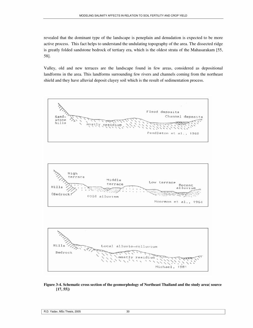
MODELING SALINIITY AFFECTS IN RELATION TO SOIL FERTILITY AND CROP YIELD
R.D. Yadav, MSc Thesis, 2005 30
revealed that the dominant type of the landscape is peneplain and denudation is expected to be more active process. This fact helps to understand the undulating topography of the area. The dissected ridge is greatly folded sandstone bedrock of tertiary era, which is the oldest strata of the Mahasarakam [55, 58]. Valley, old and new terraces are the landscape found in few areas, considered as depositional landforms in the area. This landforms surrounding few rivers and channels coming from the northeast shield and they have alluvial deposit clayey soil which is the result of sedimentation process.
Figure 3-4. Schematic cross section of the geomorphology of Northeast Thailand and the study area( source
[17, 55])
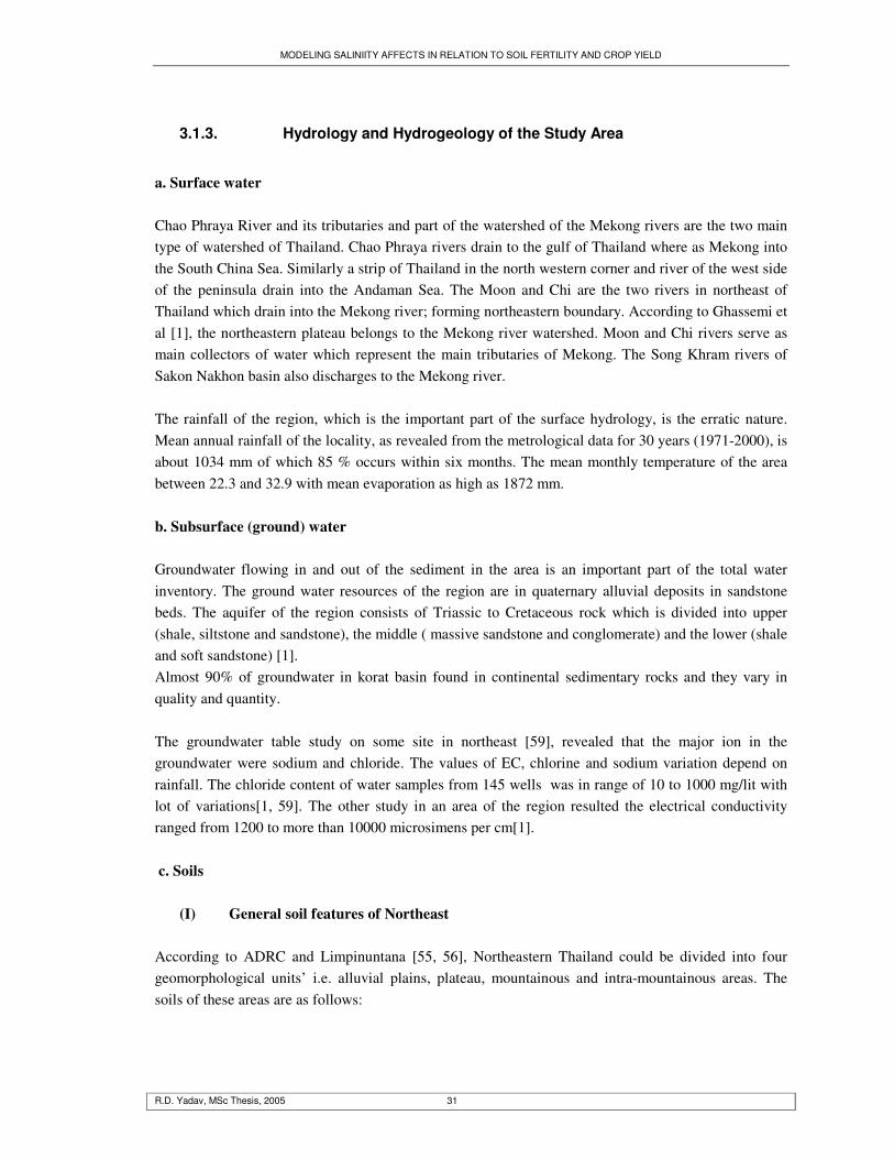
MODELING SALINIITY AFFECTS IN RELATION TO SOIL FERTILITY AND CROP YIELD
R.D. Yadav, MSc Thesis, 2005 31
3.1.3. Hydrology and Hydrogeology of the Study Area
a. Surface water Chao Phraya River and its tributaries and part of the watershed of the Mekong rivers are the two main type of watershed of Thailand. Chao Phraya rivers drain to the gulf of Thailand where as Mekong into the South China Sea. Similarly a strip of Thailand in the north western corner and river of the west side of the peninsula drain into the Andaman Sea. The Moon and Chi are the two rivers in northeast of Thailand which drain into the Mekong river; forming northeastern boundary. According to Ghassemi et al [1], the northeastern plateau belongs to the Mekong river watershed. Moon and Chi rivers serve as main collectors of water which represent the main tributaries of Mekong. The Song Khram rivers of Sakon Nakhon basin also discharges to the Mekong river. The rainfall of the region, which is the important part of the surface hydrology, is the erratic nature. Mean annual rainfall of the locality, as revealed from the metrological data for 30 years (1971-2000), is about 1034 mm of which 85 % occurs within six months. The mean monthly temperature of the area between 22.3 and 32.9 with mean evaporation as high as 1872 mm. b. Subsurface (ground) water Groundwater flowing in and out of the sediment in the area is an important part of the total water inventory. The ground water resources of the region are in quaternary alluvial deposits in sandstone beds. The aquifer of the region consists of Triassic to Cretaceous rock which is divided into upper (shale, siltstone and sandstone), the middle ( massive sandstone and conglomerate) and the lower (shale and soft sandstone) [1]. Almost 90% of groundwater in korat basin found in continental sedimentary rocks and they vary in quality and quantity. The groundwater table study on some site in northeast [59], revealed that the major ion in the groundwater were sodium and chloride. The values of EC, chlorine and sodium variation depend on rainfall. The chloride content of water samples from 145 wells was in range of 10 to 1000 mg/lit with lot of variations[1, 59]. The other study in an area of the region resulted the electrical conductivity ranged from 1200 to more than 10000 microsimens per cm[1]. c. Soils
(I) General soil features of Northeast
According to ADRC and Limpinuntana [55, 56], Northeastern Thailand could be divided into four geomorphological units’ i.e. alluvial plains, plateau, mountainous and intra-mountainous areas. The soils of these areas are as follows:

MODELING SALINIITY AFFECTS IN RELATION TO SOIL FERTILITY AND CROP YIELD
R.D. Yadav, MSc Thesis, 2005 32
a. Soils of alluvial plains Alluvial plain which is only 6% of total land area of northeast generally distributed along the Mun and Chi rivers and their tributaries along the korat basin [55]. The other areas of this plain is distributed along the Mekhong river and its tributaries in the Sakon Nakhon basin. Recent alluvial soil covers the river basin with the Ustifluvents great soil group on the natural levees and the Tropaquepts and Dystropepts on the adjacent flood plain. Ustifluvents have fine to medium texture, well drain and slightly acidic where vegetable, bamboo and fruit trees are commonly grown, [55, 56]. Tropaquepts and Dystropepts are fine textured and poorly drain that made it suitable for rice cultivation. b. Soils of the plateau The majority of the land (80%) to the Northeast falls under plateau. Basically, the basement are rocks of Mesozoic to Tertiary sandstone and silt stone of korat group[55], This give rise to the Mahasarakham formation constituting the uppermost formation as given in figure 3-2. These lands are undulating and covered by the Paleaquults and the Paleustults soils [55, 56]. These soils are characterized by sandy textured top soil. Laterite layer at shallow depth of the plateau are in 13 % of the area which lies in the Sakon Nakhon basin that falls under Plinthutults and Plinthaquults. In addition, saline and sodic soils occurrence is about 17% area of the plateau which falls under the category of Natraqualfs and Halaquepts [55, 56]. c. Soils in mountainous and intra-mountainous areas The mountainous areas which accounts to 13% of the total area on Northeast, have three mountain ranges [55]. The soils of this area could fall under the category of Paleaquults and the Paleustults and Haplustalfs in the intra-mountainous highland [55]. (II) Soils of the study area LDD staff, on the basis of USDA Soil Taxonomy has distinguished the soil of the study area into five orders (figure 3-5) [17]. The brief description of soil orders on the basis of their degree of pedogenic development is given below: a. Ultisols Ridges of the study area predominantly have “Ultisols”. These soils form with high temperature and precipitation on stable geographic surface. Low CEC and BS less than 50%, acidic nature and having low active clay characteristics keep the soil under Acrisols of WRB. The other group of WRB is Alisols characterize by acidic nature with high active clay. The “Ustic” soil moisture regime grouped the soil under “Ustults.”

MODELING SALINIITY AFFECTS IN RELATION TO SOIL FERTILITY AND CROP YIELD
R.D. Yadav, MSc Thesis, 2005 33
b. Alfisols The slopping areas adjacent to ridges as identified as glacies in the geopedologic map have Alfisols. These soils are considered as less developed compare to Ultisols as it has high base saturation percentage and leaching is less than Ultisols. Two sub-orders such as Ustalfs and Aqualfs were recognized under this order. These soils come under Lixisols of WRB system, which shows ferralic properties. c. Vertisols Vertisols occur in the northern part, around the rivers and channels of the study area. Vertic horizon formation occurs due to the presence of swelling clay minerals which consequently developed to the Vertisols. Two sub-orders Quuerts and Usterts were distinguished based on the soil moisture regime.
Figure 3-5 Soil (Series) map according to soil taxonomy 1999 , produced by LDD (Source [17]) d. Inceptisols Inceptisols are common in the lower part of the lateral valley in between the dissected ridges. The soil development of the profile is influenced by the soil forming factors interruption due to geographical position. The majority of inceptisols were classified under sub-order of Aquepts due to poor drainage condition. Poor drainage leads to develop gleyic colour with no abrupt texture group the soils under Gleysols of WRB system of soil classification. e. Entisols Entisols which are classified as Gleysols under WRB, occurred on slopping areas on few spots. They are formed from residual materials derived from the sandstone. They all belong to sub-order Psamments.

MODELING SALINIITY AFFECTS IN RELATION TO SOIL FERTILITY AND CROP YIELD
R.D. Yadav, MSc Thesis, 2005 34
3.2. Soil Salinity
Several studies have agreed that the main source of soil salinisation in northeast region is related mainly with Mahasarakham formation (salt rock) which includes the rock of salt strata [54-56]. The salt distribution in the study area shows relation with local geomorphology. Salts affected soils are concentrated mainly in lateral valley of the study area. These areas are low laying areas where salts have been accumulated from the upland area with the runoff water during the heavy precipitation. The salinity map of the study area and northeast Thailand generated by LDD is given in figure 3-6 and 3-7
Figure 3-6. (a) soil salinity map produced by Environmental science department, Thammasat university
2001 (b) cross section through the local topography after Sukchan e al c: 3D view of salinity map ([17])
Figure 3-7. Soil salinity map of northeast of Thailand (Source LDD, Khonkaen)
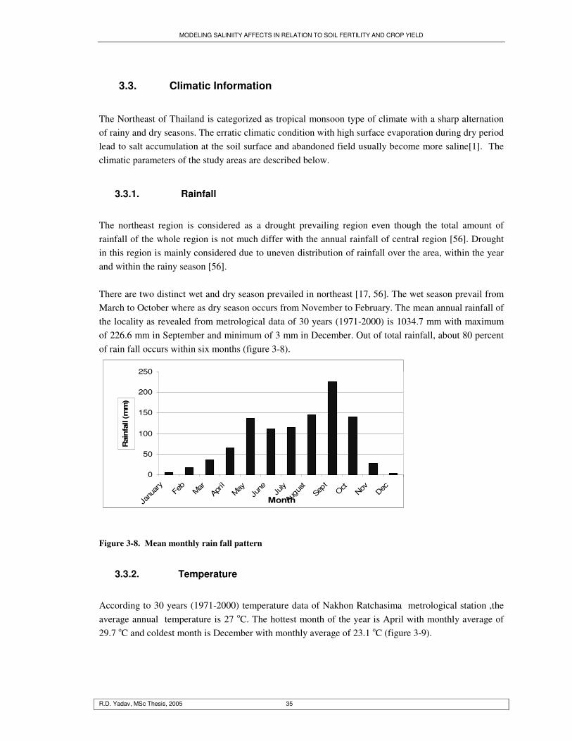
MODELING SALINIITY AFFECTS IN RELATION TO SOIL FERTILITY AND CROP YIELD
R.D. Yadav, MSc Thesis, 2005 35
3.3. Climatic Information
The Northeast of Thailand is categorized as tropical monsoon type of climate with a sharp alternation of rainy and dry seasons. The erratic climatic condition with high surface evaporation during dry period lead to salt accumulation at the soil surface and abandoned field usually become more saline[1]. The climatic parameters of the study areas are described below.
3.3.1. Rainfall
The northeast region is considered as a drought prevailing region even though the total amount of rainfall of the whole region is not much differ with the annual rainfall of central region [56]. Drought in this region is mainly considered due to uneven distribution of rainfall over the area, within the year and within the rainy season [56]. There are two distinct wet and dry season prevailed in northeast [17, 56]. The wet season prevail from March to October where as dry season occurs from November to February. The mean annual rainfall of the locality as revealed from metrological data of 30 years (1971-2000) is 1034.7 mm with maximum of 226.6 mm in September and minimum of 3 mm in December. Out of total rainfall, about 80 percent of rain fall occurs within six months (figure 3-8).
0
50
100
150
200
250
Janu
ary
Feb
MarAp
rilMay
June Ju
ly
Augu
stSe
ptOct
Nov Dec
Month
Rai
nfa
ll (m
m)
Figure 3-8. Mean monthly rain fall pattern
3.3.2. Temperature
According to 30 years (1971-2000) temperature data of Nakhon Ratchasima metrological station ,the average annual temperature is 27 oC. The hottest month of the year is April with monthly average of 29.7 oC and coldest month is December with monthly average of 23.1 oC (figure 3-9).
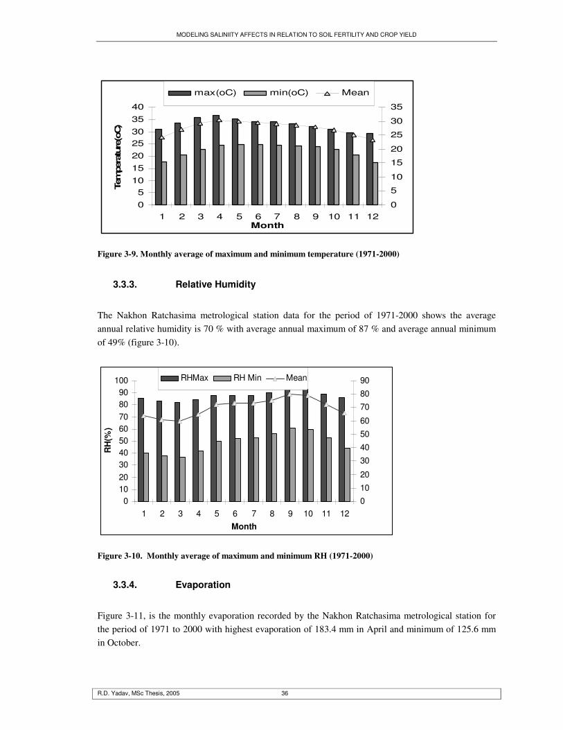
MODELING SALINIITY AFFECTS IN RELATION TO SOIL FERTILITY AND CROP YIELD
R.D. Yadav, MSc Thesis, 2005 36
05
10152025303540
1 2 3 4 5 6 7 8 9 10 11 12Month
Tem
pera
ture
(oC)
0
5
10
15
20
25
30
35
max(oC) min(oC) Mean
Figure 3-9. Monthly average of maximum and minimum temperature (1971-2000)
3.3.3. Relative Humidity
The Nakhon Ratchasima metrological station data for the period of 1971-2000 shows the average annual relative humidity is 70 % with average annual maximum of 87 % and average annual minimum of 49% (figure 3-10).
0102030405060708090
100
1 2 3 4 5 6 7 8 9 10 11 12Month
RH
(%)
01020
30405060
708090RHMax RH Min Mean
Figure 3-10. Monthly average of maximum and minimum RH (1971-2000)
3.3.4. Evaporation
Figure 3-11, is the monthly evaporation recorded by the Nakhon Ratchasima metrological station for the period of 1971 to 2000 with highest evaporation of 183.4 mm in April and minimum of 125.6 mm in October.
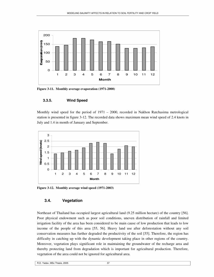
MODELING SALINIITY AFFECTS IN RELATION TO SOIL FERTILITY AND CROP YIELD
R.D. Yadav, MSc Thesis, 2005 37
0
50
100
150
200
1 2 3 4 5 6 7 8 9 10 11 12
Month
Eva
pora
tion
(mm
)
Figure 3-11. Monthly average evaporation (1971-2000)
3.3.5. Wind Speed
Monthly wind speed for the period of 1971 – 2000, recorded in Nakhon Ratchasima metrological station is presented in figure 3-12. The recorded data shows maximum mean wind speed of 2.4 knots in July and 1.4 in month of January and September.
0
0.5
1
1.5
2
2.5
3
1 2 3 4 5 6 7 8 9 10 11 12
Month
Win
d sp
eed
(kno
ts)
Figure 3-12. Monthly average wind speed (1971-2003)
3.4. Vegetation
Northeast of Thailand has occupied largest agricultural land (9.25 million hectare) of the country [56]. Poor physical endowment such as poor soil conditions, uneven distribution of rainfall and limited irrigation facility of the area has been considered to be main cause of low production that leads to low income of the people of this area [55, 56]. Heavy land use after deforestation without any soil conservation measures has further degraded the productivity of the soil [55]. Therefore, the region has difficulty in catching up with the dynamic development taking place in other regions of the country. Moreover, vegetation plays significant role in maintaining the groundwater of the recharge area and thereby protecting land from degradation which is important for agricultural production. Therefore, vegetation of the area could not be ignored for agricultural area.
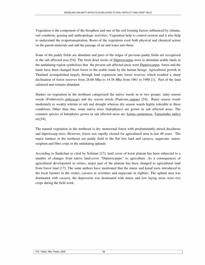
MODELING SALINIITY AFFECTS IN RELATION TO SOIL FERTILITY AND CROP YIELD
R.D. Yadav, MSc Thesis, 2005 38
Vegetation is the component of the biosphere and one of the soil forming factors influenced by climate, soil condition, grazing and anthropologic activities. Vegetation help to control erosion and it also help to understand the evapotranspiration. Roots of the vegetation exert both physical and chemical action on the parent materials and add the passage of air and water into them. Some of the paddy fields are abundant and parts of the ridges of previous paddy fields are recognized in the salt affected area [54]. The fresh dead stocks of Dipterocarpus trees in abundant arable lands in the undulating region symbolizes that the present salt affected areas were Dipterocarpus forest and the lands have been changed from forest to the arable lands by the human beings. Agricultural growth in Thailand acompalished largely through land expansion into forest reserves which resulted a sharp declination of forest reserves from 28.68 Mha to 14.38 Mha from 1961 to 1988 [1]. Part of the land salinized and remains abundant. Studies on vegetation in the northeast categorized the native weeds in to two groups: rainy season weeds (Fimbristylis milicacae) and dry season weeds (Panicum repens) [54]. Rainy season weeds moderately to weakly tolerate to salt and drought whereas dry season weeds highly tolerable to these conditions. Other than this, some native trees (halophytes) are grown in salt affected areas. The common species of halophytes grown in salt affected areas are Azima sarmentosa, Tamarindus indica etc[54]. The natural vegetation in the northeast is dry monsoonal forest with predominantly mixed deciduous and dipterocarp trees. However, forest was rapidly cleared for agricultural area in last 40 years. The major landuse in the northeast are paddy field in the flat low land and cassava, sugarcane, maize, sorghum and fibre crops in the undulating uplands According to Suukchan as cited by Soliman [17], land cover of korat plateau has been subjected to a number of changes from native land-cover “Dipterocarpus” to agriculture .As a consequences of agricultural development in sixties, major part of the plateau has been changed to agricultural land from forest land [17]. The same authors have mentioned that the maize and kenaf were introduced to the local farmers in the sixties, cassava in seventies and sugarcane in eighties. The upland area was dominated with cassava, the depression was dominated with maize and low laying areas were rice crops during the field work.
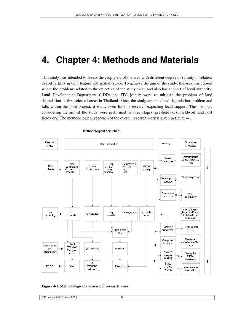
MODELING SALINIITY AFFECTS IN RELATION TO SOIL FERTILITY AND CROP YIELD
R.D. Yadav, MSc Thesis, 2005 39
4. Chapter 4: Methods and Materials
This study was intended to assess the crop yield of the area with different degree of salinity in relation to soil fertility in both feature and spatial- space. To achieve the aim of the study, the area was chosen where the problems related to the objective of the study exist, and also has support of local authority. Land Development Department (LDD) and ITC jointly work to mitigate the problem of land degradation in few selected areas in Thailand. Since the study area has land degradation problem and falls within the joint project, it was chosen for this research expecting local support. The methods, considering the aim of the study were performed in three stages: pre-fieldwork, fieldwork and post fieldwork. The methodological approach of the overall research work is given in figure 4-1
Figure 4-1. Methodological approach of research work
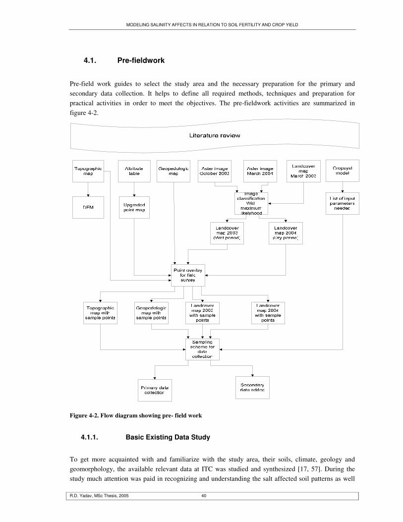
MODELING SALINIITY AFFECTS IN RELATION TO SOIL FERTILITY AND CROP YIELD
R.D. Yadav, MSc Thesis, 2005 40
4.1. Pre-fieldwork
Pre-field work guides to select the study area and the necessary preparation for the primary and secondary data collection. It helps to define all required methods, techniques and preparation for practical activities in order to meet the objectives. The pre-fieldwork activities are summarized in figure 4-2.
Figure 4-2. Flow diagram showing pre- field work
4.1.1. Basic Existing Data Study
To get more acquainted with and familiarize with the study area, their soils, climate, geology and geomorphology, the available relevant data at ITC was studied and synthesized [17, 57]. During the study much attention was paid in recognizing and understanding the salt affected soil patterns as well
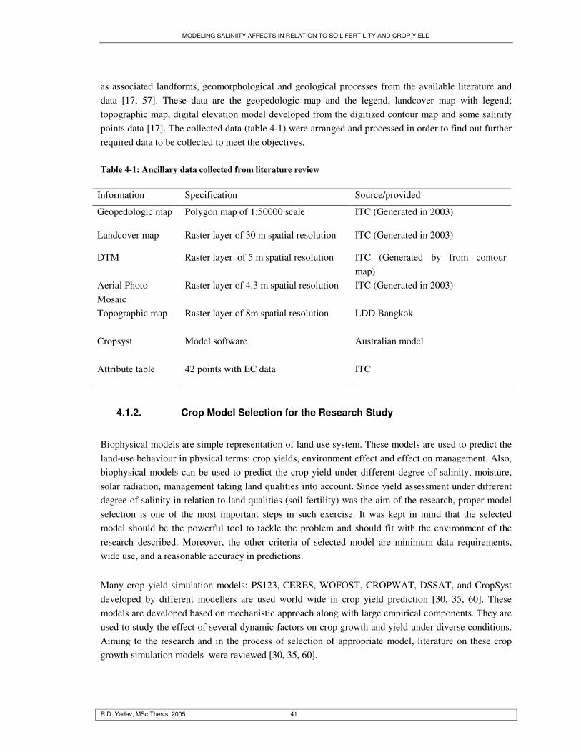
MODELING SALINIITY AFFECTS IN RELATION TO SOIL FERTILITY AND CROP YIELD
R.D. Yadav, MSc Thesis, 2005 41
as associated landforms, geomorphological and geological processes from the available literature and data [17, 57]. These data are the geopedologic map and the legend, landcover map with legend; topographic map, digital elevation model developed from the digitized contour map and some salinity points data [17]. The collected data (table 4-1) were arranged and processed in order to find out further required data to be collected to meet the objectives. Table 4-1: Ancillary data collected from literature review
Information Specification Source/provided
Geopedologic map Polygon map of 1:50000 scale ITC (Generated in 2003)
Landcover map Raster layer of 30 m spatial resolution ITC (Generated in 2003)
DTM Raster layer of 5 m spatial resolution ITC (Generated by from contour map)
Aerial Photo Mosaic
Raster layer of 4.3 m spatial resolution ITC (Generated in 2003)
Topographic map Raster layer of 8m spatial resolution LDD Bangkok
Cropsyst Model software Australian model
Attribute table 42 points with EC data ITC
4.1.2. Crop Model Selection for the Research Study
Biophysical models are simple representation of land use system. These models are used to predict the land-use behaviour in physical terms: crop yields, environment effect and effect on management. Also, biophysical models can be used to predict the crop yield under different degree of salinity, moisture, solar radiation, management taking land qualities into account. Since yield assessment under different degree of salinity in relation to land qualities (soil fertility) was the aim of the research, proper model selection is one of the most important steps in such exercise. It was kept in mind that the selected model should be the powerful tool to tackle the problem and should fit with the environment of the research described. Moreover, the other criteria of selected model are minimum data requirements, wide use, and a reasonable accuracy in predictions. Many crop yield simulation models: PS123, CERES, WOFOST, CROPWAT, DSSAT, and CropSyst developed by different modellers are used world wide in crop yield prediction [30, 35, 60]. These models are developed based on mechanistic approach along with large empirical components. They are used to study the effect of several dynamic factors on crop growth and yield under diverse conditions. Aiming to the research and in the process of selection of appropriate model, literature on these crop growth simulation models were reviewed [30, 35, 60].

MODELING SALINIITY AFFECTS IN RELATION TO SOIL FERTILITY AND CROP YIELD
R.D. Yadav, MSc Thesis, 2005 42
The WOFOST AND CERES models have been evaluated under conditions of water and/or nutrient stress considering weather, soil and phenology [60]. From the literature studied, and also keeping the aim of the study on salinity in mind, the CropSyst and PS123 model were selected. CropSyst is a user’s friendly, multi-year, multi-crop, daily time step cropping systems simulation model developed to serve as an analytical tool to study the effect of climate, soils, salinity, cropping systems management, productivity and the environment [28, 37, 61]. It is also used to simulate the soil water and nitrogen budgets, crop growth and development, crop yield, residue production and decomposition, soil erosion by water, and by salinity [28, 37, 61]. PS 123 is a user’s friendly, has facility to simulate crop yield under different degree of salinity. It considers ground water depth and ground water salinity in simulation. Therefore, this model was selected in the study where the study site has mainly groundwater salinity problems. CropSyst and PS123 models have been applied successfully in several agricultural practices assessment under different climatic conditions in different parts of the world [37, 42, 43]. The model considers the solute movement affecting crop growth; development and yield which may fulfil the aim of the study (see also chapter 2).
4.1.3. Ancillary Data Integration and Processing
The collected ancillary data (see table 4-1) were studied in detail for further processing. The data includes, a soil map at 1:50000 scale was generated in 2003 on the basis of geopedologic approach [17]. The map shares two landscapes, eight relief types, fourteen landform units and two types of lithology. The major part of the study area is peneplain whereas valley landscape forms a small part. The major relief types are ridge, glacis, vale, lateral vale, depression, flood plain, old terraces and new terraces[17]. Peneplain consists of several landforms such as top complex, side complex, slope-facet complex, summit, bottom side complex and basin under different relief types [17]. The geopedologic map was taken as the basis for data collection. The existing data of electrical conductivity of 42 points collected in 2003 [17], shared the same area were added to the database. They were arranged in the attribute table as it was one of the variables of interest of the study. The points were arranged on the basis of their coordinates. The existing topographic map of 1:50000 scale was taken as the base map. The available landcover map of 2003 [17] was considered as the basis for image classification of the provided ASTER image. The classified image was used to cover all kinds of land cover of the area for sampling. The digital elevation map generated from the contours extracted from the topographic map was also kept under database as it has information on elevation of the area and could be used whenever necessary. Aerial photographs of 1:50000 scale were available and used for the landuse monitoring purposes.
4.1.4. Data Gaps
The existing geopedologic map of the study area was used for all kinds of soil data collection. Landcover map was used along with topographic and geopedologic map for ground truthing of landuse/cover. The area has to be investigated with the existing information prior to field work. Soil property can not be measured everywhere at a well distributed manner if there are no sufficient number
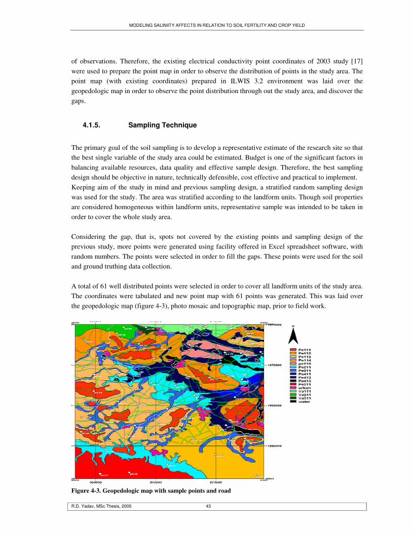
MODELING SALINIITY AFFECTS IN RELATION TO SOIL FERTILITY AND CROP YIELD
R.D. Yadav, MSc Thesis, 2005 43
of observations. Therefore, the existing electrical conductivity point coordinates of 2003 study [17] were used to prepare the point map in order to observe the distribution of points in the study area. The point map (with existing coordinates) prepared in ILWIS 3.2 environment was laid over the geopedologic map in order to observe the point distribution through out the study area, and discover the gaps.
4.1.5. Sampling Technique
The primary goal of the soil sampling is to develop a representative estimate of the research site so that the best single variable of the study area could be estimated. Budget is one of the significant factors in balancing available resources, data quality and effective sample design. Therefore, the best sampling design should be objective in nature, technically defensible, cost effective and practical to implement. Keeping aim of the study in mind and previous sampling design, a stratified random sampling design was used for the study. The area was stratified according to the landform units. Though soil properties are considered homogeneous within landform units, representative sample was intended to be taken in order to cover the whole study area. Considering the gap, that is, spots not covered by the existing points and sampling design of the previous study, more points were generated using facility offered in Excel spreadsheet software, with random numbers. The points were selected in order to fill the gaps. These points were used for the soil and ground truthing data collection. A total of 61 well distributed points were selected in order to cover all landform units of the study area. The coordinates were tabulated and new point map with 61 points was generated. This was laid over the geopedologic map (figure 4-3), photo mosaic and topographic map, prior to field work.
Figure 4-3. Geopedologic map with sample points and road
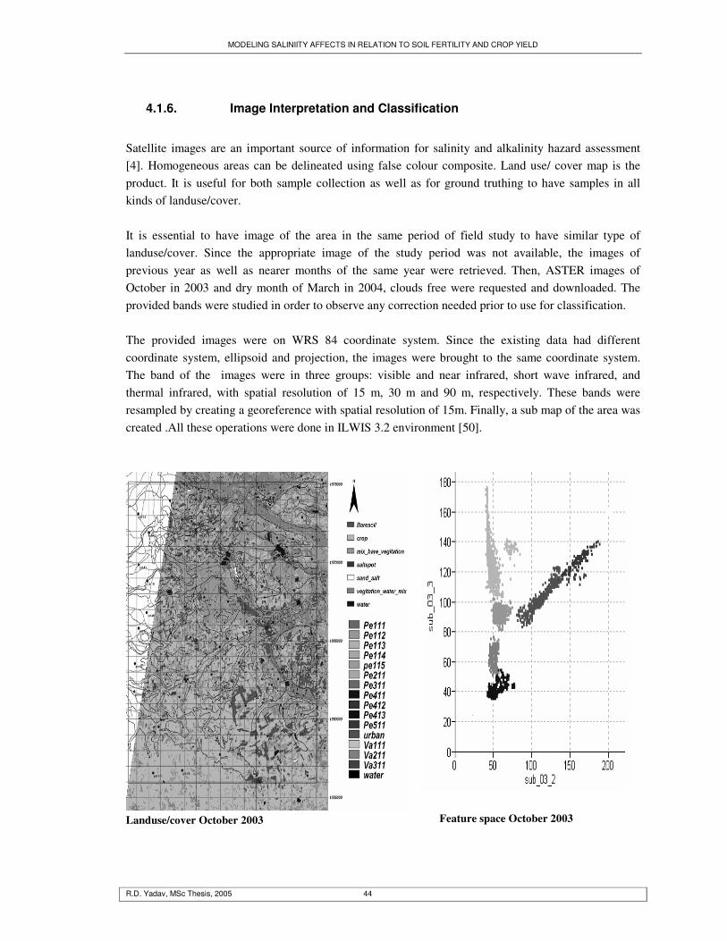
MODELING SALINIITY AFFECTS IN RELATION TO SOIL FERTILITY AND CROP YIELD
R.D. Yadav, MSc Thesis, 2005 44
4.1.6. Image Interpretation and Classification
Satellite images are an important source of information for salinity and alkalinity hazard assessment [4]. Homogeneous areas can be delineated using false colour composite. Land use/ cover map is the product. It is useful for both sample collection as well as for ground truthing to have samples in all kinds of landuse/cover. It is essential to have image of the area in the same period of field study to have similar type of landuse/cover. Since the appropriate image of the study period was not available, the images of previous year as well as nearer months of the same year were retrieved. Then, ASTER images of October in 2003 and dry month of March in 2004, clouds free were requested and downloaded. The provided bands were studied in order to observe any correction needed prior to use for classification. The provided images were on WRS 84 coordinate system. Since the existing data had different coordinate system, ellipsoid and projection, the images were brought to the same coordinate system. The band of the images were in three groups: visible and near infrared, short wave infrared, and thermal infrared, with spatial resolution of 15 m, 30 m and 90 m, respectively. These bands were resampled by creating a georeference with spatial resolution of 15m. Finally, a sub map of the area was created .All these operations were done in ILWIS 3.2 environment [50].
Landuse/cover October 2003
Feature space October 2003
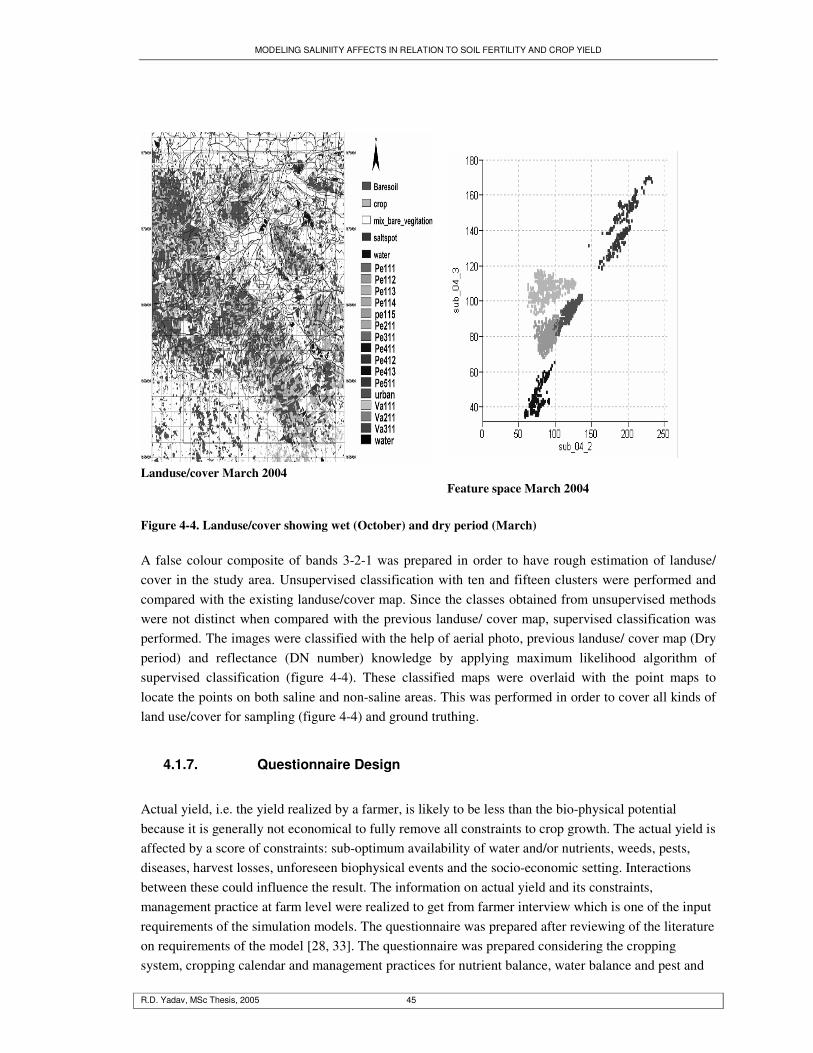
MODELING SALINIITY AFFECTS IN RELATION TO SOIL FERTILITY AND CROP YIELD
R.D. Yadav, MSc Thesis, 2005 45
Landuse/cover March 2004
Feature space March 2004
Figure 4-4. Landuse/cover showing wet (October) and dry period (March) A false colour composite of bands 3-2-1 was prepared in order to have rough estimation of landuse/ cover in the study area. Unsupervised classification with ten and fifteen clusters were performed and compared with the existing landuse/cover map. Since the classes obtained from unsupervised methods were not distinct when compared with the previous landuse/ cover map, supervised classification was performed. The images were classified with the help of aerial photo, previous landuse/ cover map (Dry period) and reflectance (DN number) knowledge by applying maximum likelihood algorithm of supervised classification (figure 4-4). These classified maps were overlaid with the point maps to locate the points on both saline and non-saline areas. This was performed in order to cover all kinds of land use/cover for sampling (figure 4-4) and ground truthing.
4.1.7. Questionnaire Design
Actual yield, i.e. the yield realized by a farmer, is likely to be less than the bio-physical potential because it is generally not economical to fully remove all constraints to crop growth. The actual yield is affected by a score of constraints: sub-optimum availability of water and/or nutrients, weeds, pests, diseases, harvest losses, unforeseen biophysical events and the socio-economic setting. Interactions between these could influence the result. The information on actual yield and its constraints, management practice at farm level were realized to get from farmer interview which is one of the input requirements of the simulation models. The questionnaire was prepared after reviewing of the literature on requirements of the model [28, 33]. The questionnaire was prepared considering the cropping system, cropping calendar and management practices for nutrient balance, water balance and pest and
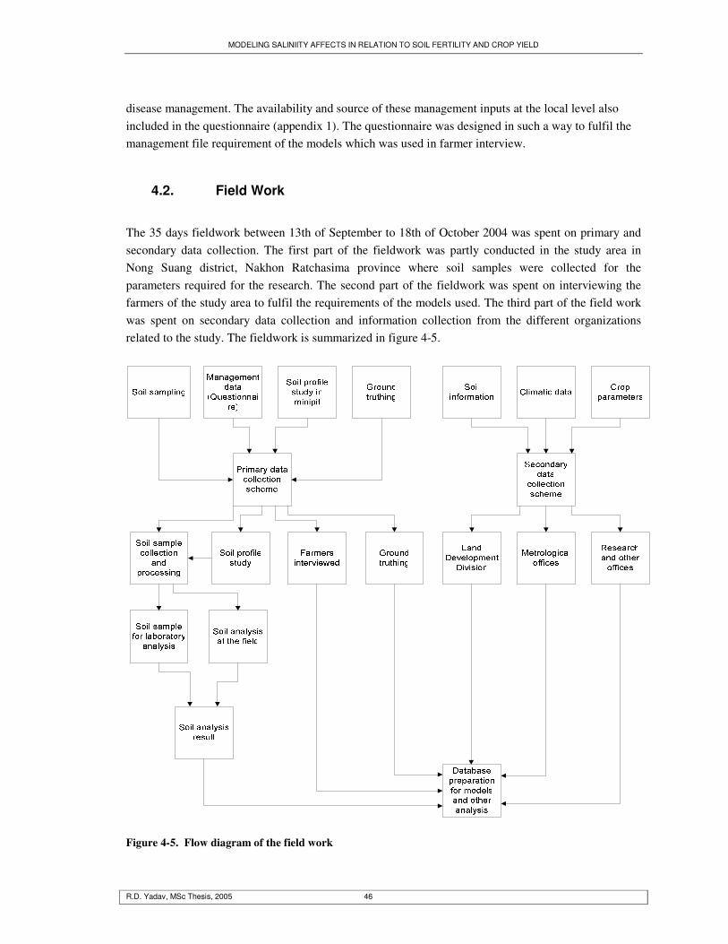
MODELING SALINIITY AFFECTS IN RELATION TO SOIL FERTILITY AND CROP YIELD
R.D. Yadav, MSc Thesis, 2005 46
disease management. The availability and source of these management inputs at the local level also included in the questionnaire (appendix 1). The questionnaire was designed in such a way to fulfil the management file requirement of the models which was used in farmer interview.
4.2. Field Work
The 35 days fieldwork between 13th of September to 18th of October 2004 was spent on primary and secondary data collection. The first part of the fieldwork was partly conducted in the study area in Nong Suang district, Nakhon Ratchasima province where soil samples were collected for the parameters required for the research. The second part of the fieldwork was spent on interviewing the farmers of the study area to fulfil the requirements of the models used. The third part of the field work was spent on secondary data collection and information collection from the different organizations related to the study. The fieldwork is summarized in figure 4-5.
Figure 4-5. Flow diagram of the field work
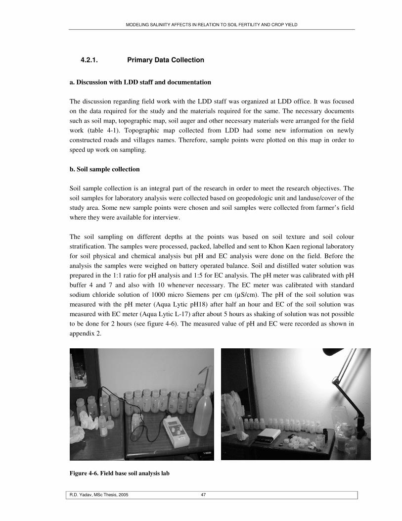
MODELING SALINIITY AFFECTS IN RELATION TO SOIL FERTILITY AND CROP YIELD
R.D. Yadav, MSc Thesis, 2005 47
4.2.1. Primary Data Collection
a. Discussion with LDD staff and documentation The discussion regarding field work with the LDD staff was organized at LDD office. It was focused on the data required for the study and the materials required for the same. The necessary documents such as soil map, topographic map, soil auger and other necessary materials were arranged for the field work (table 4-1). Topographic map collected from LDD had some new information on newly constructed roads and villages names. Therefore, sample points were plotted on this map in order to speed up work on sampling. b. Soil sample collection Soil sample collection is an integral part of the research in order to meet the research objectives. The soil samples for laboratory analysis were collected based on geopedologic unit and landuse/cover of the study area. Some new sample points were chosen and soil samples were collected from farmer’s field where they were available for interview. The soil sampling on different depths at the points was based on soil texture and soil colour stratification. The samples were processed, packed, labelled and sent to Khon Kaen regional laboratory for soil physical and chemical analysis but pH and EC analysis were done on the field. Before the analysis the samples were weighed on battery operated balance. Soil and distilled water solution was prepared in the 1:1 ratio for pH analysis and 1:5 for EC analysis. The pH meter was calibrated with pH buffer 4 and 7 and also with 10 whenever necessary. The EC meter was calibrated with standard sodium chloride solution of 1000 micro Siemens per cm (µS/cm). The pH of the soil solution was measured with the pH meter (Aqua Lytic pH18) after half an hour and EC of the soil solution was measured with EC meter (Aqua Lytic L-17) after about 5 hours as shaking of solution was not possible to be done for 2 hours (see figure 4-6). The measured value of pH and EC were recorded as shown in appendix 2.
Figure 4-6. Field base soil analysis lab
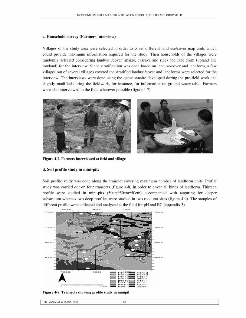
MODELING SALINIITY AFFECTS IN RELATION TO SOIL FERTILITY AND CROP YIELD
R.D. Yadav, MSc Thesis, 2005 48
c. Household survey (Farmers interview) Villages of the study area were selected in order to cover different land use/cover map units which could provide maximum information required for the study. Then households of the villages were randomly selected considering landuse /cover (maize, cassava and rice) and land form (upland and lowland) for the interview. Since stratification was done based on landuse/cover and landform, a few villages out of several villages covered the stratified landuse/cover and landforms were selected for the interview. The interviews were done using the questionnaire developed during the pre-field work and slightly modified during the fieldwork, for instance, for information on ground water table. Farmers were also interviewed in the field wherever possible (figure 4-7).
Figure 4-7. Farmers interviewed at field and village d. Soil profile study in mini-pit: Soil profile study was done along the transect covering maximum number of landform units. Profile study was carried out on four transects (figure 4-8) in order to cover all kinds of landform. Thirteen profile were studied in mini-pits (50cm*50cm*50cm) accompanied with auguring for deeper substratum whereas two deep profiles were studied in two road cut sites (figure 4-9). The samples of different profile were collected and analyzed at the field for pH and EC (appendix 3).
Figure 4-8. Transects showing profile study in minipit

MODELING SALINIITY AFFECTS IN RELATION TO SOIL FERTILITY AND CROP YIELD
R.D. Yadav, MSc Thesis, 2005 49
Figure 4-9. Soil profile study in minipit and road cut side
4.2.2. Secondary data collection
a. Climatic data
Climatic data was collected from different metrological stations in Nakhon Ratchasima province and also from the nearest metrological station such as the one in Khon Kaen. The department of meteorology, Bangkok provided some of the data (see data archived CD). However, the daily coverage of climatic data of nearby station was not obtainable; next to this province meteorological station daily data for the period of five years were collected. The climatic data of this province could be used where it has similar type of climate and elevation from the mean sea level does not vary much. This province is one of the major salts affected areas of the northeast region; having similar nature of agricultural practices. b. Soil data
Relevant soil data: soil profile information, soil series, salinity data, were collected from soil survey division of LDD Bangkok, Khon kaen, and Soil salinity division Of LDD. Similarly, some soil information data on soil profile study, soil physical and chemical properties and soil salinity were also collected from regional LDD office of Korat. c. Ground water data The ground water data of 104 wells of past in 3 to 5 different depths was collected from LDD field and central offices. About half of the wells shared the study area. They are mostly from low land salt affected area (see data archived CD).
4.3. Post Fieldwork: Data Processing and Analysis Methods
Conceptual framework (figure 4-10) was developed before entering, tabulating and processing of field collected primary and secondary data. Post fieldwork started with data entering and processing.

MODELING SALINIITY AFFECTS IN RELATION TO SOIL FERTILITY AND CROP YIELD
R.D. Yadav, MSc Thesis, 2005 50
Figure 4-10. Post fieldwork flow diagram
4.3.1. Data Preparation
a. Soil data Raw point data were entered and pre-processed in Excel spreadsheet software. The soil samples were collected on the basis of stratification of soil texture and colour in order to reduce the number of sample to minimize the analysis cost. The samples were processed for the three depths, for the variables such as EC, pH, CEC, OM and texture. They were arranged in the spreadsheet by giving the code (appendix 2). The data were output from Excel spreadsheet to SPSS format. SPSS is the statistical software which has many possibilities and easy functionalities as compared to the Excel spreadsheet for the data analysis. Therefore SPSS was used for the statistical analysis. The Excel spreadsheet is

MODELING SALINIITY AFFECTS IN RELATION TO SOIL FERTILITY AND CROP YIELD
R.D. Yadav, MSc Thesis, 2005 51
best for data base and simple calculation as compared to SPSS. Therefore, these statistical software were used wherever possible from data collection, data preparation to the data analysis. These data after preparation were input to the univariate statistics analysis (appendix 2). b. Climatic data The daily climatic data is one of the requirements of the cropsyst model which is used in this research work. The daily climatic data of 5 years (1986 to 1990) was collected from Khon kaen meteorological station. The data were entered in separate spread sheet. The missing data of days and some months of specific year were calculated by averaging the value of available days of the same months of different year where the data of other years showed similar pattern with very less variation. This data was input for the climate generation and its output was used for location file of the cropsyst model (see data archive CD). The average monthly collected climatic data of nearest meteorological station (Nakhon Ratchasima) of the study area, for the period of 1970 to 2000 (appendix 5) and also monthly data from period of 2001 to 2003 were tabulated in the spreadsheet which gives the general climatic picture of the study area. It was also used to compare the climatic data of other areas, used for the model. The monthly average of 5 years collected climatic data from central metrological department, of Packchong and Nakhon Ratchasima were arranged in the spreadsheet in tabular form for the reference (see data archive CD). c. Farmers crop management data Farmers interviewed data on crop management of the study area were extracted and processed under several columns in Excel spreadsheet. This data was later used to prepare the management input file of the model. The available information of interviewed on the basis of questionnaire were arranged in Excel spreadsheet on column name: coordinate, name of the village, planting date, harvesting date, crop yield, manure and fertilizer (appendix 6). d. Crop data Since the model requires biophysical parameters: classification, crop growth, crop morphology, crop phenology, and harvesting parameters of crop, were collected from secondary source. The model requires many biophysical parameters which was one of the constraints faced during data collection. The collected biophysical parameters from the field and literature were arranged in Excel spread sheet which is the input for the cropsyst model.
4.3.2. Exploratory Data Analysis
It is the precursory stage to observe the statistical properties of the data. This technique showed the applicability and usefulness of visualizing data and calculating simple statistics as a preliminary stage to confirmatory tests. The statistical analysis part is summarized in figure 4-11

MODELING SALINIITY AFFECTS IN RELATION TO SOIL FERTILITY AND CROP YIELD
R.D. Yadav, MSc Thesis, 2005 52
Figure 4-11. Summary of non-spatial statistical analysis
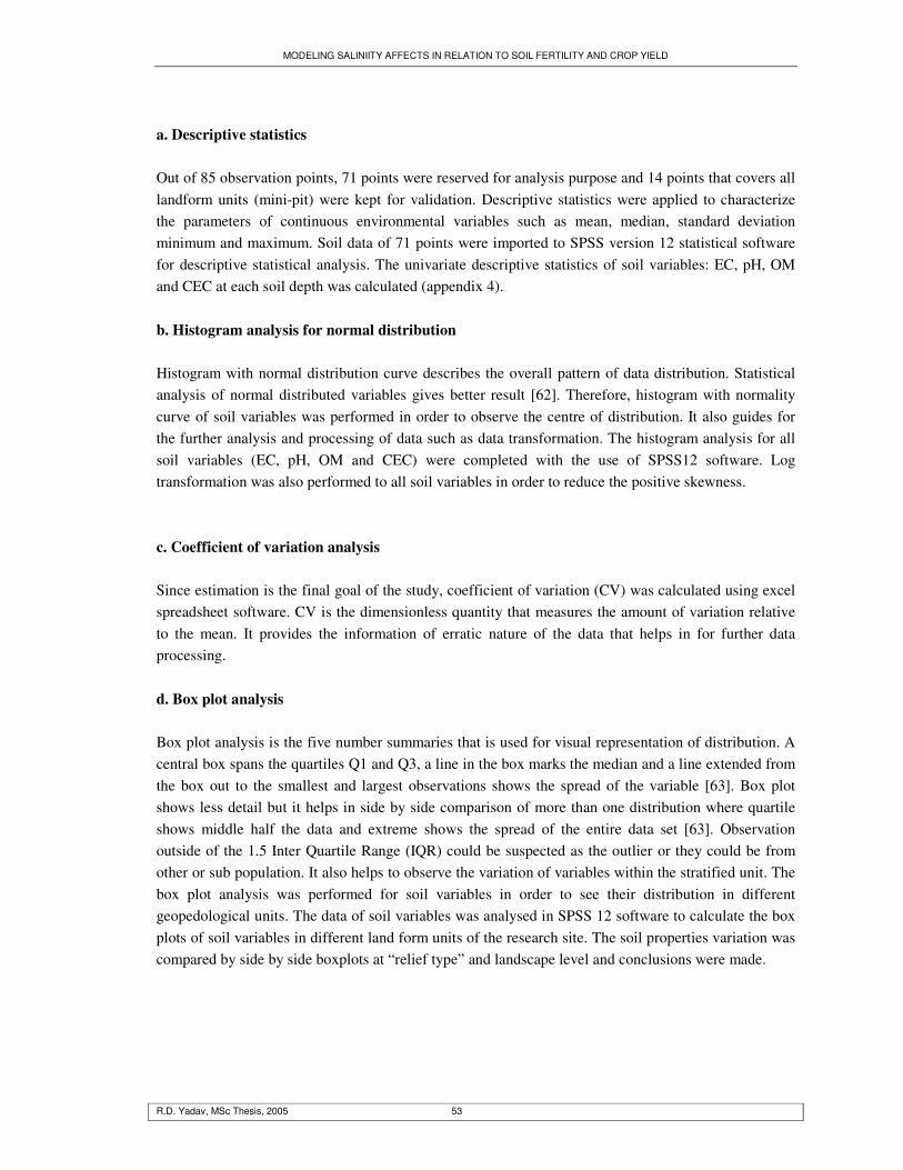
MODELING SALINIITY AFFECTS IN RELATION TO SOIL FERTILITY AND CROP YIELD
R.D. Yadav, MSc Thesis, 2005 53
a. Descriptive statistics Out of 85 observation points, 71 points were reserved for analysis purpose and 14 points that covers all landform units (mini-pit) were kept for validation. Descriptive statistics were applied to characterize the parameters of continuous environmental variables such as mean, median, standard deviation minimum and maximum. Soil data of 71 points were imported to SPSS version 12 statistical software for descriptive statistical analysis. The univariate descriptive statistics of soil variables: EC, pH, OM and CEC at each soil depth was calculated (appendix 4). b. Histogram analysis for normal distribution Histogram with normal distribution curve describes the overall pattern of data distribution. Statistical analysis of normal distributed variables gives better result [62]. Therefore, histogram with normality curve of soil variables was performed in order to observe the centre of distribution. It also guides for the further analysis and processing of data such as data transformation. The histogram analysis for all soil variables (EC, pH, OM and CEC) were completed with the use of SPSS12 software. Log transformation was also performed to all soil variables in order to reduce the positive skewness. c. Coefficient of variation analysis Since estimation is the final goal of the study, coefficient of variation (CV) was calculated using excel spreadsheet software. CV is the dimensionless quantity that measures the amount of variation relative to the mean. It provides the information of erratic nature of the data that helps in for further data processing. d. Box plot analysis Box plot analysis is the five number summaries that is used for visual representation of distribution. A central box spans the quartiles Q1 and Q3, a line in the box marks the median and a line extended from the box out to the smallest and largest observations shows the spread of the variable [63]. Box plot shows less detail but it helps in side by side comparison of more than one distribution where quartile shows middle half the data and extreme shows the spread of the entire data set [63]. Observation outside of the 1.5 Inter Quartile Range (IQR) could be suspected as the outlier or they could be from other or sub population. It also helps to observe the variation of variables within the stratified unit. The box plot analysis was performed for soil variables in order to see their distribution in different geopedological units. The data of soil variables was analysed in SPSS 12 software to calculate the box plots of soil variables in different land form units of the research site. The soil properties variation was compared by side by side boxplots at “relief type” and landscape level and conclusions were made.
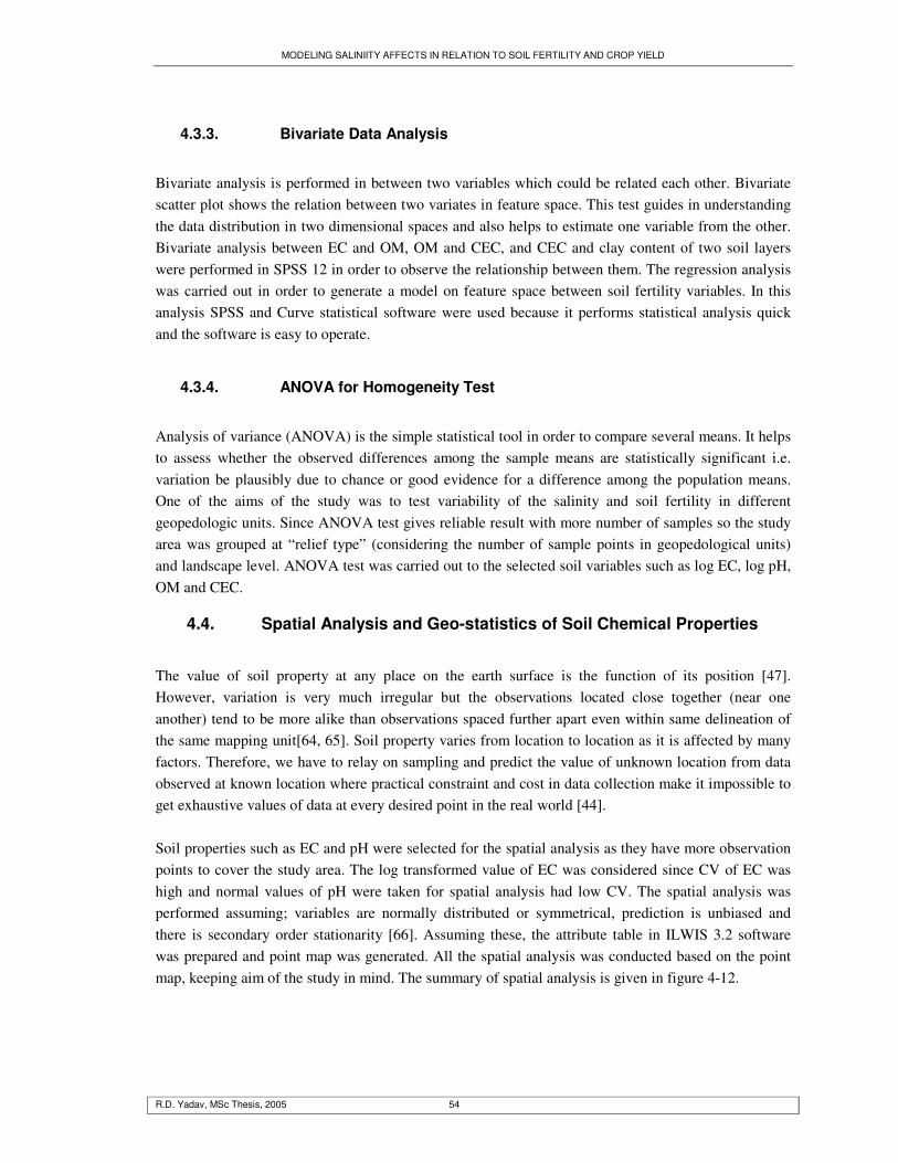
MODELING SALINIITY AFFECTS IN RELATION TO SOIL FERTILITY AND CROP YIELD
R.D. Yadav, MSc Thesis, 2005 54
4.3.3. Bivariate Data Analysis
Bivariate analysis is performed in between two variables which could be related each other. Bivariate scatter plot shows the relation between two variates in feature space. This test guides in understanding the data distribution in two dimensional spaces and also helps to estimate one variable from the other. Bivariate analysis between EC and OM, OM and CEC, and CEC and clay content of two soil layers were performed in SPSS 12 in order to observe the relationship between them. The regression analysis was carried out in order to generate a model on feature space between soil fertility variables. In this analysis SPSS and Curve statistical software were used because it performs statistical analysis quick and the software is easy to operate.
4.3.4. ANOVA for Homogeneity Test
Analysis of variance (ANOVA) is the simple statistical tool in order to compare several means. It helps to assess whether the observed differences among the sample means are statistically significant i.e. variation be plausibly due to chance or good evidence for a difference among the population means. One of the aims of the study was to test variability of the salinity and soil fertility in different geopedologic units. Since ANOVA test gives reliable result with more number of samples so the study area was grouped at “relief type” (considering the number of sample points in geopedological units) and landscape level. ANOVA test was carried out to the selected soil variables such as log EC, log pH, OM and CEC.
4.4. Spatial Analysis and Geo-statistics of Soil Chemical Properties
The value of soil property at any place on the earth surface is the function of its position [47]. However, variation is very much irregular but the observations located close together (near one another) tend to be more alike than observations spaced further apart even within same delineation of the same mapping unit[64, 65]. Soil property varies from location to location as it is affected by many factors. Therefore, we have to relay on sampling and predict the value of unknown location from data observed at known location where practical constraint and cost in data collection make it impossible to get exhaustive values of data at every desired point in the real world [44]. Soil properties such as EC and pH were selected for the spatial analysis as they have more observation points to cover the study area. The log transformed value of EC was considered since CV of EC was high and normal values of pH were taken for spatial analysis had low CV. The spatial analysis was performed assuming; variables are normally distributed or symmetrical, prediction is unbiased and there is secondary order stationarity [66]. Assuming these, the attribute table in ILWIS 3.2 software was prepared and point map was generated. All the spatial analysis was conducted based on the point map, keeping aim of the study in mind. The summary of spatial analysis is given in figure 4-12.
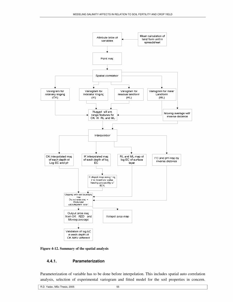
MODELING SALINIITY AFFECTS IN RELATION TO SOIL FERTILITY AND CROP YIELD
R.D. Yadav, MSc Thesis, 2005 55
Figure 4-12. Summary of the spatial analysis
4.4.1. Parameterization
Parameterization of variable has to be done before interpolation. This includes spatial auto correlation analysis, selection of experimental variogram and fitted model for the soil properties in concern.

MODELING SALINIITY AFFECTS IN RELATION TO SOIL FERTILITY AND CROP YIELD
R.D. Yadav, MSc Thesis, 2005 56
Estimation of features such as nugget, sill and range are important in interpolation. These parameters were used in interpolation from the point data to prepare the map of the concern variables. This technique has been considered as an appropriate for soil variables which was the aim of this study to prepare the soil salinity and soil fertility map in order to observe their pattern in space. Parameterization of ordinary Kriging for log EC and pH Spatial auto correlation analysis was carried out by selecting the appropriate lag-distance with 71 points data of log EC and pH of each depth. The features of the fitted models (Nugget, sill and range) were estimated by selecting different experimental variogram model by assigning the values for nugget, sill and range with fitted variogram. The fitted variogram models were tested with R2 in ILWIS 3.2 environment.
4.4.2. KED (Kriging with External Drift)
KED is a mixed interpolator that includes feature-space predictors that are not geographic coordinates. KED and UK (universal Kriging) are having same mathematics but they do differ in base function [66]. The base function in UK refers to the grid coordinate whereas it is referred to feature space covariates in KED that measures at sample points [66]. There are two kinds of feature space in KED. They are strata (factors) and continuous covariates. Error variance can be minimized with KED where it considers local variance within each stratum and global within strata. Since soil properties such as log EC showed significant difference in geopedologic unit, kriging with external drift (KED) which includes feature space predictors that are not on geographic coordinates i.e. it implies a feature space process independent of residuals [66] may give better estimates. KED of log EC of surface layer of soil was performed to compare the result with OK and moving average (inverse distance square) of same depth. Parameterization of KED of log EC30 for surface layer of soil The data set of log EC30 was grouped according to landform units. Mean of landform units were calculated in spread sheet which was placed in the attribute table of ILWIS 3.2 software along the landform units of log EC 30 value. Residual value of each landform unit was calculated by giving the command in command line of the attribute table (Residual=column name of variables minus mean of variables). Then residual and mean experimental variogram with their features were estimated. The fitted model was tested with R2 in ILWIS software.
4.4.3. Interpolation
Kriging can be considered as a point interpolation method. It requires the point map as input and output is the raster map with estimation with optionally error map. Necessary parameters (weight factors) to run the kriging are those, determined by specified variogram model based on spatial correlation outputs (see also chapter 2).

MODELING SALINIITY AFFECTS IN RELATION TO SOIL FERTILITY AND CROP YIELD
R.D. Yadav, MSc Thesis, 2005 57
Interpolation methods such as moving average (inverse distance) which was applied in the study, is a local estimator, calculate the arithmetic average for a central point within a predefined neighbourhood (i.e. moving window with a certain limiting distance). It assumes that each input point has a local influence that diminishes with the distance. It weights the points closer to the processing cell greater than those farther away [64, 67]. A specified number of points or optionally all points within a specified radius can be used to determine the output values for each location. More input points and well their distribution give more reliable results. It predicts the values for cells in a raster from a limited number of sample data points. It can be used to predict the unknown values for any geographic points data: soil properties, elevation, rainfall, chemical concentration and noise levels [64, 67]. Interpolation methods such as moving average (inverse distance) and Ordinary Kriging with their feature parameters were performed for Log EC and pH for each soil depth. Interpolation was done in ILWIS 3.2 environment.
In order to have KED map, semi-variogram and parameters of residual and mean were used for interpolation to have residual logEC30 and mean logEC30 map. These maps were generated in ILWIS 3.2 environment. Further, these maps were added to generate KED map, giving the command, KED=residual logEC30+ Mean logEC30. All interpolated maps were clipped with boundary map (digitized from the geopedologic map) by giving command IFFNOTUNDEF (BOUNDARY, MAP). Finally interpolated map of the area of log EC and pH were produced.
4.5. Hot Spot Map Preparation
Hotspots are the indicators for the particular variable having higher probability beyond the threshold value. It gives the area having probability value of parameters beyond their threshold value. For instance, most of the field crops severely affected beyond ECe level 8 dS/m. If hotspot map has been prepared giving threshold value 8 dS/m for ECe with 60 % or more probability level, then such hot spot area would have 60 or more percent chances of ECe value 8 dS/m. If any, crop wants to grow in such an area, there could be 60 or more percent chances to have ECe effect on crop growth and yield. It means, chances of crop failure are higher in hot spot areas and it may not be suitable for the particular crops meeting this threshold level. The threshold value selected for the study area was more than 2 dS/cm as most of the field crops in the areas has an adverse effect on growth and yield beyond this value [68]. The EC value greater than this, was given 1 and lower than 2 dS/m was given 0 in command line of the attribute table. Then spatial correlation table and fitted variogram were generated with their estimated features in ILWIS environment. The indicator kriging interpolation was done with the variogram features, which gives the probability of getting the threshold EC value in the study area. Then the hotspot map was made by selecting the area having more than 80% probability of EC value beyond the threshold with the help of command in ILWIS software.

MODELING SALINIITY AFFECTS IN RELATION TO SOIL FERTILITY AND CROP YIELD
R.D. Yadav, MSc Thesis, 2005 58
4.6. Salinity and Soil Reaction (Ph) Map Preparation
The interpolated map from moving average (inverse distance square) for both variables (logEC and pH) was considered to prepare salinity and soil reaction in order to analyze the changes of these with depths. The salinity class map was generated by slicing operation in ILWIS 3.2 environment. The EC map was divided into five salinity classes as non saline, slightly saline, moderately saline, strong saline and extremely saline as shown in figure 5-11 (a-c) [68]. Similarly, pH map was classified into soil reaction classes by providing pH range value for acidity and alkalinity (figure5-12, a-c) [69].
4.7. Landuse/cover Map Preparation
Landuse/cover map is necessary to integrate the model output to the spatial extent in order to assess the yield of the area. The ASTER image having spatial resolution of 15 m which was collected during the pre-field work was used for landuse/cover map making. Since the appropriate image of the study period was not available, the available image of ASTER image for the period of October 2003 free from cloud was selected on an assumption that the landuse/cover was same during the image acquisition date. Visible and near infra red bands were selected for the colour composite. The false colour composite of bands 3-2-1 was prepared which was the best combination for vegetation identification. Since ground truth points were collected from the field, supervised classification technique was applied to train the sample based on the ground truthing. The sample set was created and sample was trained. Once the sample was trained, further task was to select the appropriate image classifier algorithms to classify the image. There are several image classifier algoritham: box classifier, minimum distance to cluster mean classifier and maximum likelihood available in the software for the classification of image [50]. Considering feature space of the trained sample for the spectral pattern of various classes, maximum likelihood classifier algorithm was selected. Assuming normal distribution of the training data set, statistical parameters: means, variance and covariance, the given pixel is assigned to the particular class. Finally, image was classified by applying maximum likelihood algorithm of supervised classification and landuse/cover map was made. All operation was carried out in ILWIS 3.2 environment [50]. The output of the classification contained some noises. This could be spectral overlap in the sample set or because of improper training by classifier. These noises can be removed by filtering technique. Majority filter was considered as an appropriate filter which does not alter the original pixel value and it was applied to remove the noises of the classified image.
4.8. Crop Growth Model and GIS Integration in Yield Modelling
4.8.1. Input File Preparation for the CropSyst Model
Five input data files: Location, Soil, Crop, and Management are required to run CropSyst simulation control. The required data and files and simulation process are described in figure 4-13.
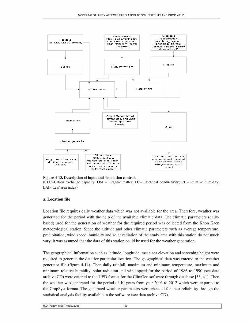
MODELING SALINIITY AFFECTS IN RELATION TO SOIL FERTILITY AND CROP YIELD
R.D. Yadav, MSc Thesis, 2005 59
Figure 4-13. Description of input and simulation control. (CEC=Cation exchange capacity; OM = Organic matter; EC= Electrical conductivity; RH= Relative humidity; LAI= Leaf area index)
a. Location file Location file requires daily weather data which was not available for the area. Therefore, weather was generated for the period with the help of the available climatic data. The climatic parameters (daily- based) used for the generation of weather for the required period was collected from the Khon Kaen meteorological station. Since the altitude and other climatic parameters such as average temperature, precipitation, wind speed, humidity and solar radiation of the study area with this station do not much vary, it was assumed that the data of this station could be used for the weather generation. The geographical information such as latitude, longitude, mean sea elevation and screening height were required to generate the data for particular location. The geographical data was entered to the weather generator file (figure 4-14). Then daily rainfall, maximum and minimum temperature, maximum and minimum relative humidity, solar radiation and wind speed for the period of 1986 to 1990 (see data archive CD) were entered to the UED format for the ClimGen software through database [33, 41]. Then the weather was generated for the period of 10 years from year 2003 to 2012 which were exported to the CropSyst format. The generated weather parameters were checked for their reliability through the statistical analysis facility available in the software (see data archive CD).
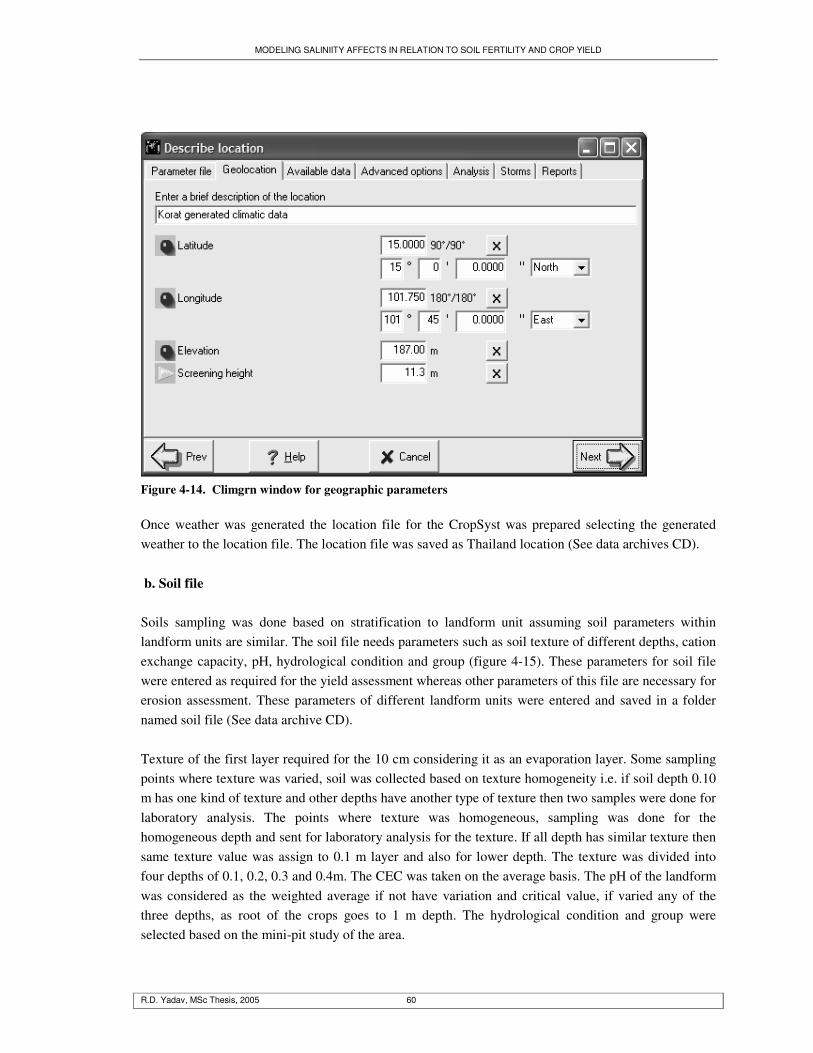
MODELING SALINIITY AFFECTS IN RELATION TO SOIL FERTILITY AND CROP YIELD
R.D. Yadav, MSc Thesis, 2005 60
Figure 4-14. Climgrn window for geographic parameters Once weather was generated the location file for the CropSyst was prepared selecting the generated weather to the location file. The location file was saved as Thailand location (See data archives CD). b. Soil file Soils sampling was done based on stratification to landform unit assuming soil parameters within landform units are similar. The soil file needs parameters such as soil texture of different depths, cation exchange capacity, pH, hydrological condition and group (figure 4-15). These parameters for soil file were entered as required for the yield assessment whereas other parameters of this file are necessary for erosion assessment. These parameters of different landform units were entered and saved in a folder named soil file (See data archive CD). Texture of the first layer required for the 10 cm considering it as an evaporation layer. Some sampling points where texture was varied, soil was collected based on texture homogeneity i.e. if soil depth 0.10 m has one kind of texture and other depths have another type of texture then two samples were done for laboratory analysis. The points where texture was homogeneous, sampling was done for the homogeneous depth and sent for laboratory analysis for the texture. If all depth has similar texture then same texture value was assign to 0.1 m layer and also for lower depth. The texture was divided into four depths of 0.1, 0.2, 0.3 and 0.4m. The CEC was taken on the average basis. The pH of the landform was considered as the weighted average if not have variation and critical value, if varied any of the three depths, as root of the crops goes to 1 m depth. The hydrological condition and group were selected based on the mini-pit study of the area.
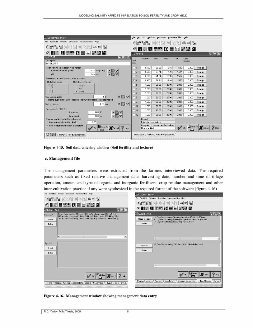
MODELING SALINIITY AFFECTS IN RELATION TO SOIL FERTILITY AND CROP YIELD
R.D. Yadav, MSc Thesis, 2005 61
Figure 4-15. Soil data entering window (Soil fertility and texture) c. Management file The management parameters were extracted from the farmers interviewed data. The required parameters such as fixed relative management date, harvesting date, number and time of tillage operation, amount and type of organic and inorganic fertilizers, crop residue management and other inter-cultivation practice if any were synthesized in the required format of the software (figure 4-16).
Figure 4-16. Management window showing management data entry
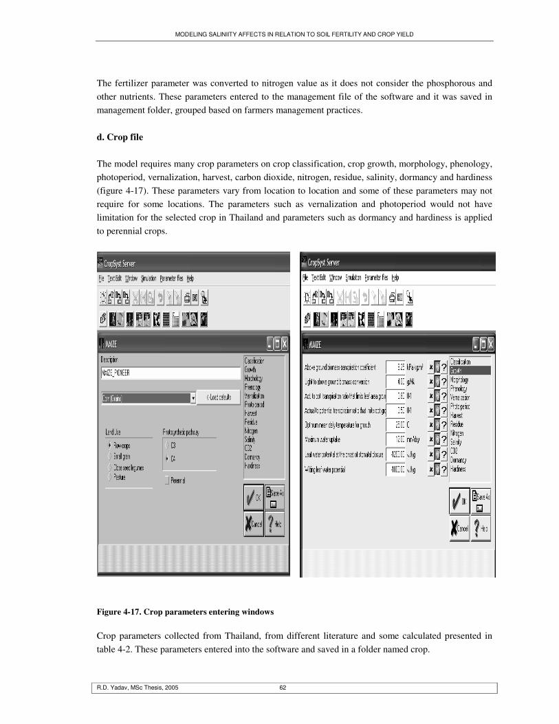
MODELING SALINIITY AFFECTS IN RELATION TO SOIL FERTILITY AND CROP YIELD
R.D. Yadav, MSc Thesis, 2005 62
The fertilizer parameter was converted to nitrogen value as it does not consider the phosphorous and other nutrients. These parameters entered to the management file of the software and it was saved in management folder, grouped based on farmers management practices. d. Crop file The model requires many crop parameters on crop classification, crop growth, morphology, phenology, photoperiod, vernalization, harvest, carbon dioxide, nitrogen, residue, salinity, dormancy and hardiness (figure 4-17). These parameters vary from location to location and some of these parameters may not require for some locations. The parameters such as vernalization and photoperiod would not have limitation for the selected crop in Thailand and parameters such as dormancy and hardiness is applied to perennial crops.
Figure 4-17. Crop parameters entering windows Crop parameters collected from Thailand, from different literature and some calculated presented in table 4-2. These parameters entered into the software and saved in a folder named crop.
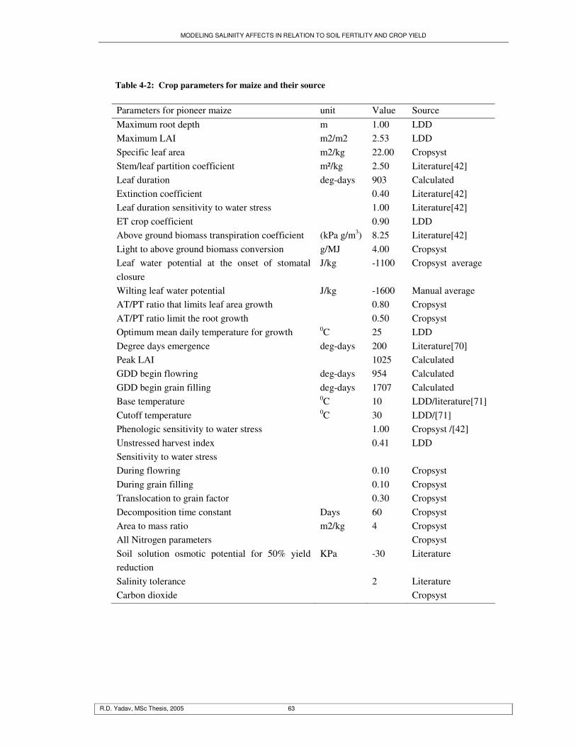
MODELING SALINIITY AFFECTS IN RELATION TO SOIL FERTILITY AND CROP YIELD
R.D. Yadav, MSc Thesis, 2005 63
Table 4-2: Crop parameters for maize and their source
Parameters for pioneer maize unit Value Source Maximum root depth m 1.00 LDD Maximum LAI m2/m2 2.53 LDD Specific leaf area m2/kg 22.00 Cropsyst Stem/leaf partition coefficient m²/kg 2.50 Literature[42] Leaf duration deg-days 903 Calculated Extinction coefficient 0.40 Literature[42] Leaf duration sensitivity to water stress 1.00 Literature[42] ET crop coefficient 0.90 LDD Above ground biomass transpiration coefficient (kPa g/m3) 8.25 Literature[42] Light to above ground biomass conversion g/MJ 4.00 Cropsyst Leaf water potential at the onset of stomatal closure
J/kg -1100 Cropsyst average
Wilting leaf water potential J/kg -1600 Manual average AT/PT ratio that limits leaf area growth 0.80 Cropsyst AT/PT ratio limit the root growth 0.50 Cropsyst Optimum mean daily temperature for growth 0C 25 LDD Degree days emergence deg-days 200 Literature[70] Peak LAI 1025 Calculated GDD begin flowring deg-days 954 Calculated GDD begin grain filling deg-days 1707 Calculated Base temperature 0C 10 LDD/literature[71] Cutoff temperature 0C 30 LDD/[71] Phenologic sensitivity to water stress 1.00 Cropsyst /[42] Unstressed harvest index 0.41 LDD Sensitivity to water stress During flowring During grain filling
0.10 0.10
Cropsyst Cropsyst
Translocation to grain factor 0.30 Cropsyst Decomposition time constant Days 60 Cropsyst Area to mass ratio m2/kg 4 Cropsyst All Nitrogen parameters Cropsyst Soil solution osmotic potential for 50% yield reduction
KPa -30 Literature
Salinity tolerance 2 Literature Carbon dioxide Cropsyst
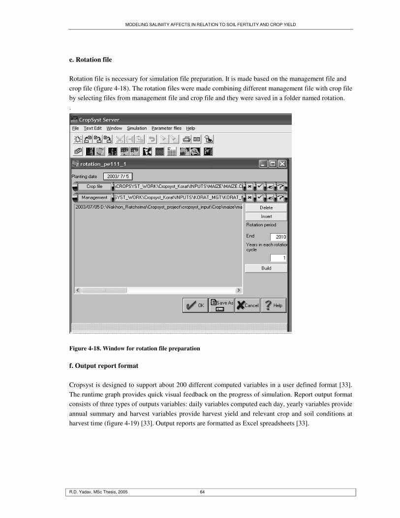
MODELING SALINIITY AFFECTS IN RELATION TO SOIL FERTILITY AND CROP YIELD
R.D. Yadav, MSc Thesis, 2005 64
e. Rotation file Rotation file is necessary for simulation file preparation. It is made based on the management file and crop file (figure 4-18). The rotation files were made combining different management file with crop file by selecting files from management file and crop file and they were saved in a folder named rotation. .
Figure 4-18. Window for rotation file preparation f. Output report format Cropsyst is designed to support about 200 different computed variables in a user defined format [33]. The runtime graph provides quick visual feedback on the progress of simulation. Report output format consists of three types of outputs variables: daily variables computed each day, yearly variables provide annual summary and harvest variables provide harvest yield and relevant crop and soil conditions at harvest time (figure 4-19) [33]. Output reports are formatted as Excel spreadsheets [33].
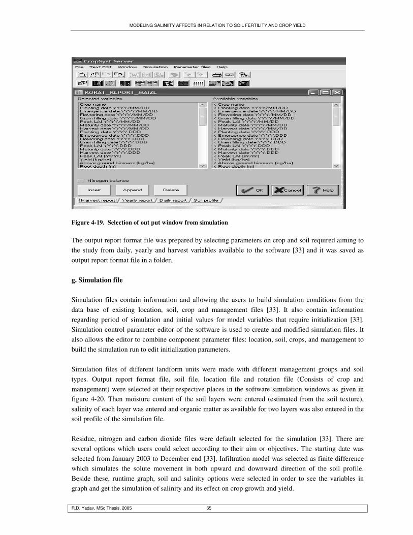
MODELING SALINIITY AFFECTS IN RELATION TO SOIL FERTILITY AND CROP YIELD
R.D. Yadav, MSc Thesis, 2005 65
Figure 4-19. Selection of out put window from simulation The output report format file was prepared by selecting parameters on crop and soil required aiming to the study from daily, yearly and harvest variables available to the software [33] and it was saved as output report format file in a folder. g. Simulation file Simulation files contain information and allowing the users to build simulation conditions from the data base of existing location, soil, crop and management files [33]. It also contain information regarding period of simulation and initial values for model variables that require initialization [33]. Simulation control parameter editor of the software is used to create and modified simulation files. It also allows the editor to combine component parameter files: location, soil, crops, and management to build the simulation run to edit initialization parameters. Simulation files of different landform units were made with different management groups and soil types. Output report format file, soil file, location file and rotation file (Consists of crop and management) were selected at their respective places in the software simulation windows as given in figure 4-20. Then moisture content of the soil layers were entered (estimated from the soil texture), salinity of each layer was entered and organic matter as available for two layers was also entered in the soil profile of the simulation file. Residue, nitrogen and carbon dioxide files were default selected for the simulation [33]. There are several options which users could select according to their aim or objectives. The starting date was selected from January 2003 to December end [33]. Infiltration model was selected as finite difference which simulates the solute movement in both upward and downward direction of the soil profile. Beside these, runtime graph, soil and salinity options were selected in order to see the variables in graph and get the simulation of salinity and its effect on crop growth and yield.
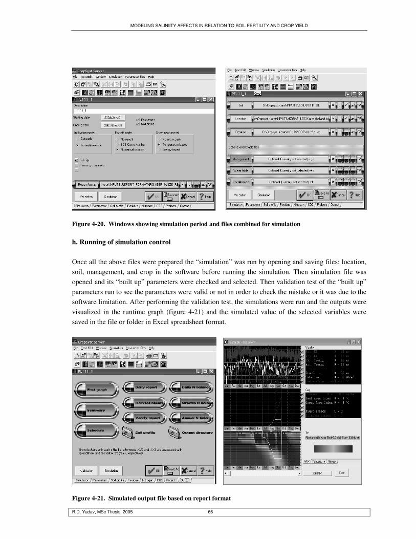
MODELING SALINIITY AFFECTS IN RELATION TO SOIL FERTILITY AND CROP YIELD
R.D. Yadav, MSc Thesis, 2005 66
Figure 4-20. Windows showing simulation period and files combined for simulation h. Running of simulation control Once all the above files were prepared the “simulation” was run by opening and saving files: location, soil, management, and crop in the software before running the simulation. Then simulation file was opened and its “built up” parameters were checked and selected. Then validation test of the “built up” parameters run to see the parameters were valid or not in order to check the mistake or it was due to the software limitation. After performing the validation test, the simulations were run and the outputs were visualized in the runtime graph (figure 4-21) and the simulated value of the selected variables were saved in the file or folder in Excel spreadsheet format.
Figure 4-21. Simulated output file based on report format

MODELING SALINIITY AFFECTS IN RELATION TO SOIL FERTILITY AND CROP YIELD
R.D. Yadav, MSc Thesis, 2005 67
4.8.2. Input File Preparation for PS123
Three main input data files: Climate, Soil, and Crop, are required to run PS 123 crop growth model. These files are sequential ASCII files that can be easily be made or altered with most editors (edlin, EDIT, programme editor, Norton editor etc.) [40]. Beside these, it also required data on management: seed rate, planting time and soil ground water table. The required data and files and simulation process are described in figure 4-22.
Figure 4-22. Summary of crop growth simulation under sub model PS 2 a. Climate file Climate file of the PS 123 consists of two lines: Line # 1, encloses site name, latitude (degree), longitude (degree) and elevation from mean sea level (meter). Line # 2 encloses Julian day number; daily maximum temperature (Tmax oC and minimum temperature (Tmin oC), daily precipitation (PREC cm d-1); mean daily relative humidity (RHA 0-1), daily potential evaporation (Eo cm d-1), sunshine hour (SUNH h d-1) and daily potential evapotranspiration (ETo cm d-
1). Climate file was prepared with 2003 available climatic data of meteorological station. Since, all required climatic parameters were not available at one station; relevant data from other nearby stations were used to prepare the climate file. Since the altitude and other climatic parameters such as average temperature, precipitation, wind speed, humidity and solar radiation of the study area do not much vary with this (nearer) station, it was assumed that the data of this station could be used for the climate file. The nearest (20 km) meteorological station (Nakhon Ratchasima) climatic parameters such as
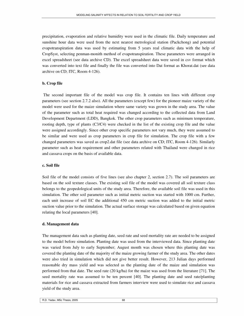
MODELING SALINIITY AFFECTS IN RELATION TO SOIL FERTILITY AND CROP YIELD
R.D. Yadav, MSc Thesis, 2005 68
precipitation, evaporation and relative humidity were used in the climatic file. Daily temperature and sunshine hour data were used from the next nearest metrological station (Packchong) and potential evapotranspiration data was used by estimating from 5 years real climatic data with the help of CropSyst, selecting penman-monith method of evapotranspiration. These parameters were arranged in excel spreadsheet (see data archive CD). The excel spreadsheet data were saved in csv format which was converted into text file and finally the file was converted into Dat format as Khorat.dat (see data archive on CD; ITC, Room 4-126). b. Crop file The second important file of the model was crop file. It contains ten lines with different crop parameters (see section 2.7.2 also). All the parameters (except few) for the pioneer maize variety of the model were used for the maize simulation where same variety was grown in the study area. The value of the parameter such as total heat required was changed according to the collected data from Land Development Department (LDD), Bangkok. The other crop parameters such as minimum temperature, rooting depth, type of plants (C3/C4) were checked in the list of the existing crop file and the value were assigned accordingly. Since other crop specific parameters not vary much, they were assumed to be similar and were used as crop parameters in crop file for simulation. The crop file with a few changed parameters was saved as crop2.dat file (see data archive on CD; ITC, Room 4-126). Similarly parameter such as heat requirement and other parameters related with Thailand were changed in rice and cassava crops on the basis of available data. c. Soil file Soil file of the model consists of five lines (see also chapter 2, section 2.7). The soil parameters are based on the soil texture classes. The existing soil file of the model was covered all soil texture class belongs to the geopedological units of the study area. Therefore, the available soil file was used in this simulation. The other soil parameter such as initial metric suction was started with 1000 cm. Further, each unit increase of soil EC the additional 450 cm metric suction was added to the initial metric suction value prior to the simulation. The actual surface storage was calculated based on given equation relating the local parameters [40]. d. Management data The management data such as planting date, seed rate and seed mortality rate are needed to be assigned to the model before simulation. Planting date was used from the interviewed data. Since planting date was varied from July to early September; August month was chosen where this planting date was covered the planting date of the majority of the maize growing farmer of the study area. The other dates were also tried in simulation which did not give better result. However, 213 Julian days performed reasonable dry mass yield and was selected as the planting date of the maize and simulation was performed from that date. The seed rate (20 kg/ha) for the maize was used from the literature [71]. The seed mortality rate was assumed to be ten percent [40]. The planting date and seed rate/planting materials for rice and cassava extracted from farmers interview were used to simulate rice and cassava yield of the study area.
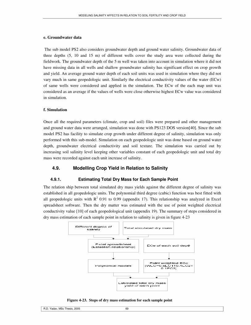
MODELING SALINIITY AFFECTS IN RELATION TO SOIL FERTILITY AND CROP YIELD
R.D. Yadav, MSc Thesis, 2005 69
e. Groundwater data The sub model PS2 also considers groundwater depth and ground water salinity. Groundwater data of three depths (5, 10 and 15 m) of different wells cover the study area were collected during the fieldwork. The groundwater depth of the 5 m well was taken into account in simulation where it did not have missing data in all wells and shallow groundwater salinity has significant effect on crop growth and yield. An average ground water depth of each soil units was used in simulation where they did not vary much in same geopedologic unit. Similarly the electrical conductivity values of the water (ECw) of same wells were considered and applied in the simulation. The ECw of the each map unit was considered as an average if the values of wells were close otherwise highest ECw value was considered in simulation. f. Simulation Once all the required parameters (climate, crop and soil) files were prepared and other management and ground water data were arranged, simulation was done with PS123 DOS version[40]. Since the sub model PS2 has facility to simulate crop growth under different degree of salinity, simulation was only performed with this sub-model. Simulation on each geopedologic unit was done based on ground water depth, groundwater electrical conductivity and soil texture. The simulation was carried out by increasing soil salinity level keeping other variables constant of each geopedologic unit and total dry mass were recorded against each unit increase of salinity.
4.9. Modelling Crop Yield in Relation to Salinity
4.9.1. Estimating Total Dry Mass for Each Sample Point
The relation ship between total simulated dry mass yields against the different degree of salinity was established in all geopedologic units. The polynomial third degree (cubic) function was best fitted with all geopedologic units with R2 0.91 to 0.99 (appendix 17). This relationship was analyzed in Excel spreadsheet software. Then the dry matter was estimated with the use of point weighted electrical conductivity value [10] of each geopedological unit (appendix 19). The summary of steps considered in dry mass estimation of each sample point in relation to salinity is given in figure 4-23
Figure 4-23. Steps of dry mass estimation for each sample point

MODELING SALINIITY AFFECTS IN RELATION TO SOIL FERTILITY AND CROP YIELD
R.D. Yadav, MSc Thesis, 2005 70
4.9.2. Modelling Crop Yield
The overall crop modelling steps is given in figure 4-24. Dry mass attribute table of yield of each sample point including their coordinates was prepared in ILWIS 3.2 environment. The dry mass yield point map was prepared from the attribute table and interpolation was performed by moving average (inverse distance square) because moving average among the other methods was best explained the salinity of the area.
Figure 4-24. Flow diagram showing the steps for preparing yield map Note: (*) IFF(Lcover= crop, crop,?);
(**) iffnotundef (map boundary, interpolated map) (***) Drymatter map* HI (Harvesting index)
The interpolated map was clipped with the boundary map in order to get interpolated area map. Then yield map was prepared by multiplying the dry matter map with the harvesting index (0.41), collected from LDD, Bangkok. Further, interpolated yield map was classified by slicing operation with the yield domain: <1 mt/ha, 1-2 mt/ha, 2-3 mt/ha, 3-4 mt/ha, 4-5 mt/ha, 5-6 mt/ha and >6 mt/ha. The separate crop cover map of maize was obtained through masking the landcover map with IFF operation. After
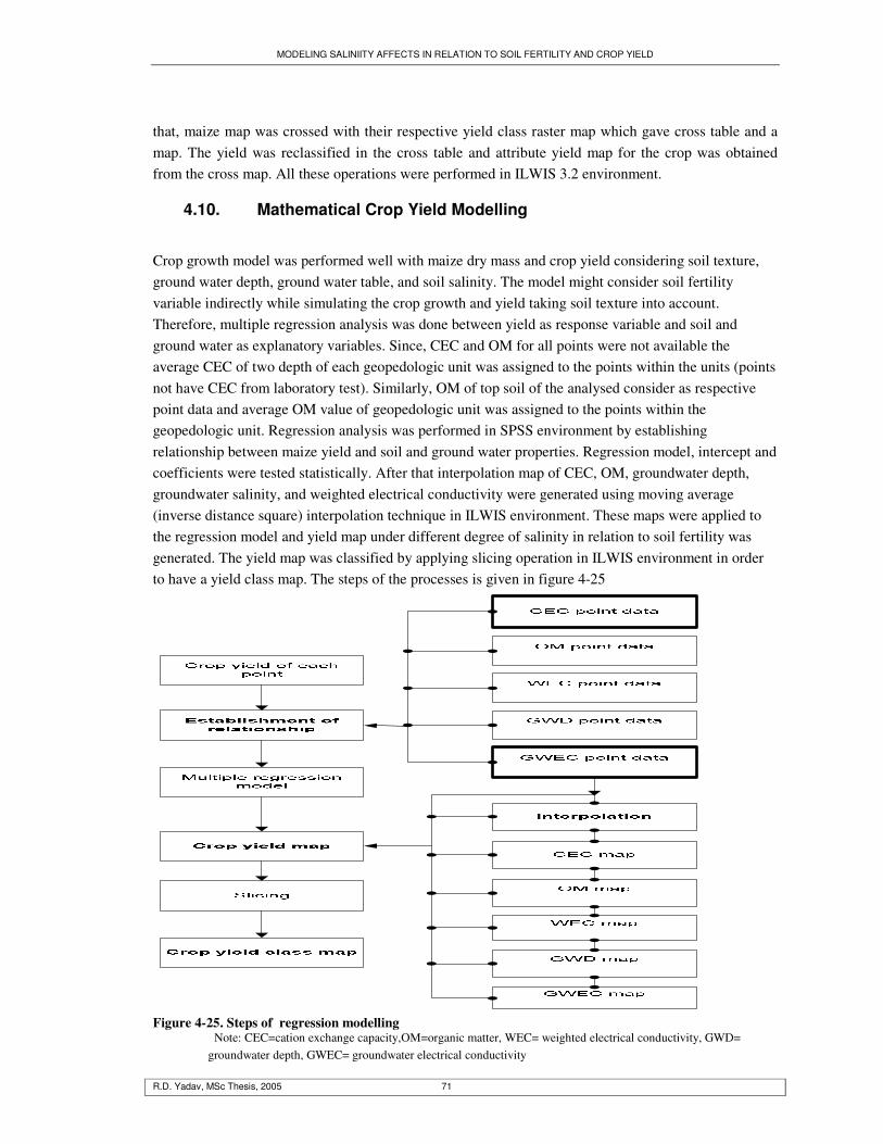
MODELING SALINIITY AFFECTS IN RELATION TO SOIL FERTILITY AND CROP YIELD
R.D. Yadav, MSc Thesis, 2005 71
that, maize map was crossed with their respective yield class raster map which gave cross table and a map. The yield was reclassified in the cross table and attribute yield map for the crop was obtained from the cross map. All these operations were performed in ILWIS 3.2 environment.
4.10. Mathematical Crop Yield Modelling
Crop growth model was performed well with maize dry mass and crop yield considering soil texture, ground water depth, ground water table, and soil salinity. The model might consider soil fertility variable indirectly while simulating the crop growth and yield taking soil texture into account. Therefore, multiple regression analysis was done between yield as response variable and soil and ground water as explanatory variables. Since, CEC and OM for all points were not available the average CEC of two depth of each geopedologic unit was assigned to the points within the units (points not have CEC from laboratory test). Similarly, OM of top soil of the analysed consider as respective point data and average OM value of geopedologic unit was assigned to the points within the geopedologic unit. Regression analysis was performed in SPSS environment by establishing relationship between maize yield and soil and ground water properties. Regression model, intercept and coefficients were tested statistically. After that interpolation map of CEC, OM, groundwater depth, groundwater salinity, and weighted electrical conductivity were generated using moving average (inverse distance square) interpolation technique in ILWIS environment. These maps were applied to the regression model and yield map under different degree of salinity in relation to soil fertility was generated. The yield map was classified by applying slicing operation in ILWIS environment in order to have a yield class map. The steps of the processes is given in figure 4-25
Figure 4-25. Steps of regression modelling
Note: CEC=cation exchange capacity,OM=organic matter, WEC= weighted electrical conductivity, GWD= groundwater depth, GWEC= groundwater electrical conductivity
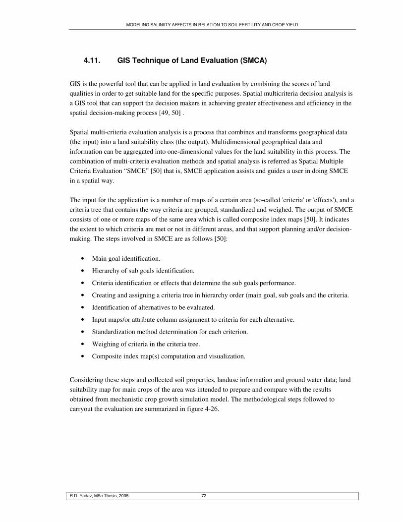
MODELING SALINIITY AFFECTS IN RELATION TO SOIL FERTILITY AND CROP YIELD
R.D. Yadav, MSc Thesis, 2005 72
4.11. GIS Technique of Land Evaluation (SMCA)
GIS is the powerful tool that can be applied in land evaluation by combining the scores of land qualities in order to get suitable land for the specific purposes. Spatial multicriteria decision analysis is a GIS tool that can support the decision makers in achieving greater effectiveness and efficiency in the spatial decision-making process [49, 50] . Spatial multi-criteria evaluation analysis is a process that combines and transforms geographical data (the input) into a land suitability class (the output). Multidimensional geographical data and information can be aggregated into one-dimensional values for the land suitability in this process. The combination of multi-criteria evaluation methods and spatial analysis is referred as Spatial Multiple Criteria Evaluation “SMCE” [50] that is, SMCE application assists and guides a user in doing SMCE in a spatial way. The input for the application is a number of maps of a certain area (so-called 'criteria' or 'effects'), and a criteria tree that contains the way criteria are grouped, standardized and weighed. The output of SMCE consists of one or more maps of the same area which is called composite index maps [50]. It indicates the extent to which criteria are met or not in different areas, and that support planning and/or decision-making. The steps involved in SMCE are as follows [50]:
• Main goal identification.
• Hierarchy of sub goals identification.
• Criteria identification or effects that determine the sub goals performance.
• Creating and assigning a criteria tree in hierarchy order (main goal, sub goals and the criteria.
• Identification of alternatives to be evaluated.
• Input maps/or attribute column assignment to criteria for each alternative.
• Standardization method determination for each criterion.
• Weighing of criteria in the criteria tree.
• Composite index map(s) computation and visualization.
Considering these steps and collected soil properties, landuse information and ground water data; land suitability map for main crops of the area was intended to prepare and compare with the results obtained from mechanistic crop growth simulation model. The methodological steps followed to carryout the evaluation are summarized in figure 4-26.
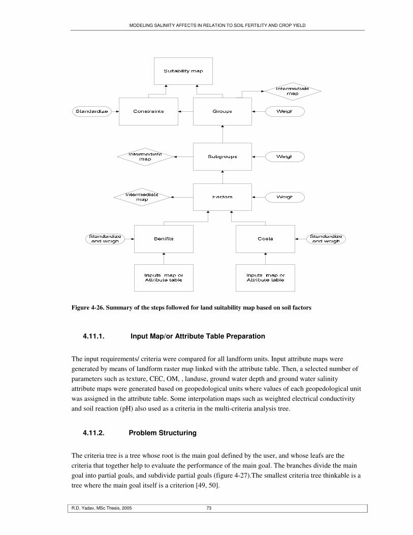
MODELING SALINIITY AFFECTS IN RELATION TO SOIL FERTILITY AND CROP YIELD
R.D. Yadav, MSc Thesis, 2005 73
Figure 4-26. Summary of the steps followed for land suitability map based on soil factors
4.11.1. Input Map/or Attribute Table Preparation
The input requirements/ criteria were compared for all landform units. Input attribute maps were generated by means of landform raster map linked with the attribute table. Then, a selected number of parameters such as texture, CEC, OM, , landuse, ground water depth and ground water salinity attribute maps were generated based on geopedological units where values of each geopedological unit was assigned in the attribute table. Some interpolation maps such as weighted electrical conductivity and soil reaction (pH) also used as a criteria in the multi-criteria analysis tree.
4.11.2. Problem Structuring
The criteria tree is a tree whose root is the main goal defined by the user, and whose leafs are the criteria that together help to evaluate the performance of the main goal. The branches divide the main goal into partial goals, and subdivide partial goals (figure 4-27).The smallest criteria tree thinkable is a tree where the main goal itself is a criterion [49, 50].
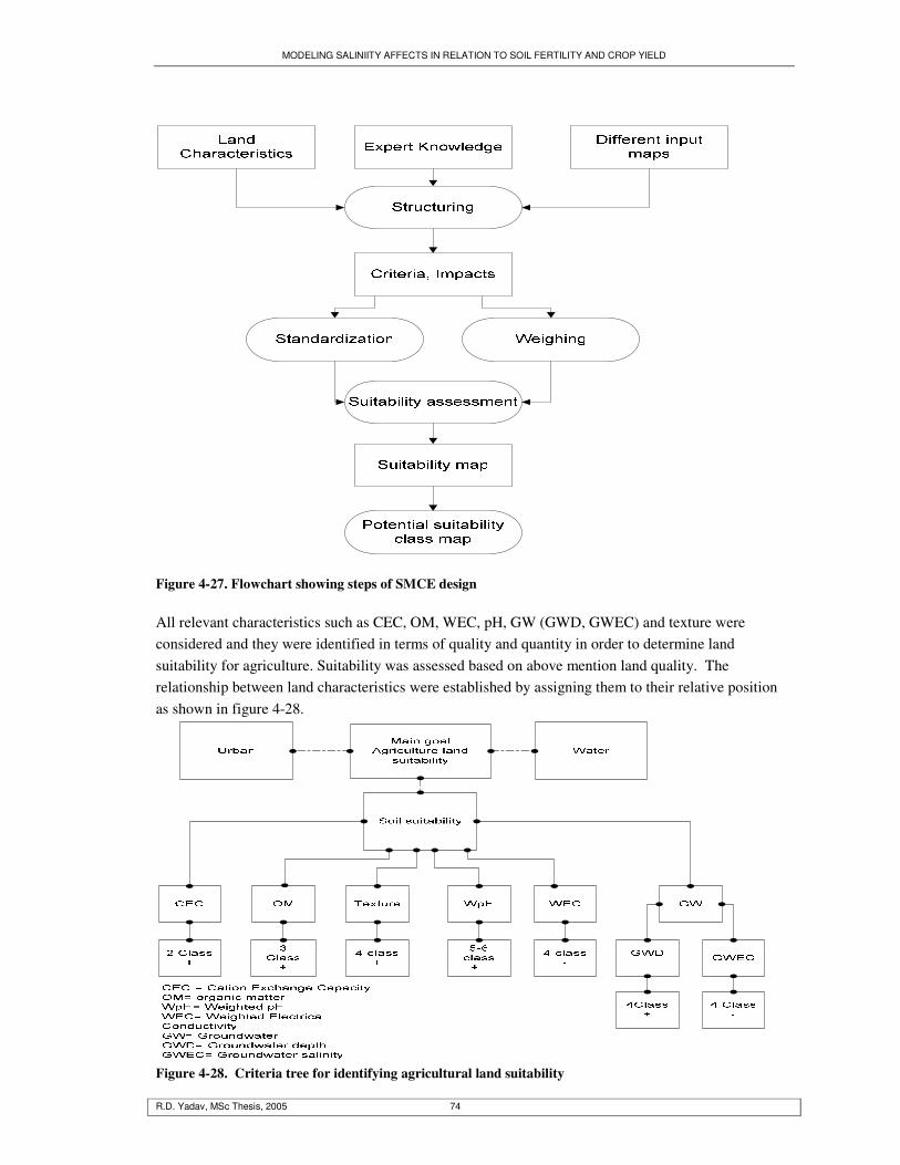
MODELING SALINIITY AFFECTS IN RELATION TO SOIL FERTILITY AND CROP YIELD
R.D. Yadav, MSc Thesis, 2005 74
Figure 4-27. Flowchart showing steps of SMCE design All relevant characteristics such as CEC, OM, WEC, pH, GW (GWD, GWEC) and texture were considered and they were identified in terms of quality and quantity in order to determine land suitability for agriculture. Suitability was assessed based on above mention land quality. The relationship between land characteristics were established by assigning them to their relative position as shown in figure 4-28.
Figure 4-28. Criteria tree for identifying agricultural land suitability
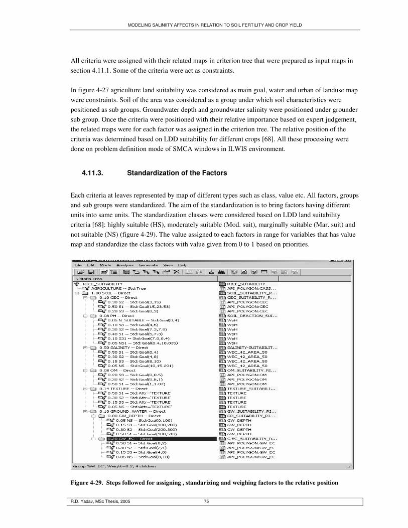
MODELING SALINIITY AFFECTS IN RELATION TO SOIL FERTILITY AND CROP YIELD
R.D. Yadav, MSc Thesis, 2005 75
All criteria were assigned with their related maps in criterion tree that were prepared as input maps in section 4.11.1. Some of the criteria were act as constraints. In figure 4-27 agriculture land suitability was considered as main goal, water and urban of landuse map were constraints. Soil of the area was considered as a group under which soil characteristics were positioned as sub groups. Groundwater depth and groundwater salinity were positioned under grounder sub group. Once the criteria were positioned with their relative importance based on expert judgement, the related maps were for each factor was assigned in the criterion tree. The relative position of the criteria was determined based on LDD suitability for different crops [68]. All these processing were done on problem definition mode of SMCA windows in ILWIS environment.
4.11.3. Standardization of the Factors
Each criteria at leaves represented by map of different types such as class, value etc. All factors, groups and sub groups were standardized. The aim of the standardization is to bring factors having different units into same units. The standardization classes were considered based on LDD land suitability criteria [68]: highly suitable (HS), moderately suitable (Mod. suit), marginally suitable (Mar. suit) and not suitable (NS) (figure 4-29). The value assigned to each factors in range for variables that has value map and standardize the class factors with value given from 0 to 1 based on priorities.
Figure 4-29. Steps followed for assigning , standarizing and weighing factors to the relative position

MODELING SALINIITY AFFECTS IN RELATION TO SOIL FERTILITY AND CROP YIELD
R.D. Yadav, MSc Thesis, 2005 76
4.11.4. Weighing of Criteria in the Criteria Tree
Identification of relative importance of each indicator called weights [49]. When the main goal contains multiple factors and optional sub goals, then the main goal needs to be weighed based on their relative importance (factors, goals, and sub goals) of the containing factors with respect to the main goal. Similarly, when a sub goal (group) contains multiple factors and more optional sub goals, then it also needs to be weighed in order to indicate the relative importance of the factors (and optional sub goals) it contains, with respect to the sub goal. The weighing was done from the lowest group of the hierarchy order. The weighing was based on the priority in between score 0 to 1.Therefore, ground water depth and ground water salinity were first to be weighed as they were at the last position of the hierarchy order in the tree. Then sub groups ground water, texture, OM, salinity, and CEC were weighed. Further, soil group was weighed. Once weighing was completed, final land suitability map of different crops along with their intermediate map were generated in ILWIS environment. After that the map was classified in four classes such as highly suitable (0.75-1.0), moderately suitable (0.50-0.75), marginally suitable (0.25-0.50) and not suitable (0-0.25) by slicing operation in ILWIS3.2 environment.
4.12. Sensitivity Analysis
Sensitivity analysis is the method to test the sensitiveness of the model by changing one parameter keeping others constant. The sensitivity analysis was conducted by selecting dominant maize growing geopedologic unit (PE 511). The unit falls under depression and having loamy sand texture with low CEC (7.20) and low pH (5.05). Maize is planted during the month of July as rainfed crop. Farmers practiced two tillage operations (one a month prior to planting and other at the day of planting). They were used complete blended type of different grade fertilizer (15-15-15; 16-8-8, etc) with almost no organic manure. The fertilizer was calculated in terms of total nitrogen per hectare. The phenologic development of the crop was calculated based on the output date of different stage of the maize of DSSAT. The data were collected from the LDD in Bangkok during the fieldwork. The climatic parameters were used also the simulated values from the DSAT. The phenology growth degree days was calculated with the help of crop calibrator of CropSyst. The salinity value was selected only for the surface layer of the soil. The model was run by changing the EC value from 1 to 20 dS/m and tabulated the yield against EC value.

MODELING SALINIITY AFFECTS IN RELATION TO SOIL FERTILITY AND CROP YIELD
R.D. Yadav, MSc Thesis, 2005 77
5. Chapter 5: Results and Discussion
In this chapter, the results obtained from the analytical methods of the data are presented and discussed. It deals with non-spatial and spatial analysis by the application of relevant statistical methods and image classification. Also crop yield as affected by salinity in relation to soil fertility are simulated. The results are then integrated in GIS domain. Within the GIS domain several maps were generated among which are soil salinity hotspots, soil reaction, and suitability areas in relation to salinity levels for growing selected crops.
5.1. Spatial Distribution of Soil Properties
In a study to predict or map out hotspots, it is necessary to estimate the reliability and behaviour of the data to be used. This can lead to precision. Therefore spatial correlation methods were applied to estimate the nature of soil properties as they are distributed in geopedological units. The results from the application of univariate, bivariate and ANOVA are described as follows:
5.1.1. Spatial Nature of Soil Properties
The nature of the data of the distribution of soil properties in pedologic units became apparently clear after applying descriptive statistical analysis of the given dataset. In precision, central tendencies, the measure of locations were estimated as the mean and median of the data. Further, measures of variability range, quartile, and standard deviation were applied to the dataset.
The results of univariate analysis of soil variables (appendix 4) indicated that the means of the variables were slightly higher than the medians with coefficient varying from 0.4 to 4.6 exhibited positive skewness. Standard deviation in the variables shows variation. The results are an indication that the dataset is not normally distributed.
. The higher variation of the soil properties such as electrical conductivity (EC), OM, and CEC in each soil depth could be inferred from the standard deviation. The variability of the pH shows small as it possesses the lesser standard deviation. The difference between minimum and maximum values of the variables gives the range. The range value of CEC, pH, EC and OM are listed from highest to lowest (appendix 4).
The erratic nature of data or the skeweness of data could result to an unreliable output. Therefore coefficient of variation (CV) which shows the erratic behaviour of datasets was applied to find out to

MODELING SALINIITY AFFECTS IN RELATION TO SOIL FERTILITY AND CROP YIELD
R.D. Yadav, MSc Thesis, 2005 78
which extend the data is erratic and to serve as a guide for further analysis. If CV is greater than 100 percent an indication may the presence of samples with erratic values. The presence of erratic values is an indication of outliers but the rejection of outliers on a purely statistical basis could be dangerous as the high or low values belong to a certain location of particular landform. It could be possible to represent these as sub-population. Outliers are normal occurrence in soil dataset where soil property depend on factors such as climate, parent material, relative position of the landscape, vegetation, ground water table and depth and human activities which vary from point to point in landscapes.
The analysis revealed that EC had higher CV pointing out that EC may vary with soil depth whereas pH and OM do not show high variations with depth (figure 5-1). The findings arouse interest to find out the variation between depths (0-30, 30-60 and 60-90) cm. Comparing the variation of EC between depths of soil the surface layer (0-30) showed much variation but the variation decreased with depth as indicated by decreasing CV with depth. Similarly, CEC of surface soil layer showed higher variation with depth that can be linked to variation in clay content, because clay content increase with depth. This indicates that there is direct relationship between EC and clay content.
0
50
100
150
200
250
300
350
0-30 30-60 60-90
Depth
CV %
EC
pH
OM
CEC
Figure 5-1. Coefficient of variation of variables in three and two depth The histogram with normal distribution curve of soil variables (appendices 9, 10 and 11) showed that all the soil variables analysed were not normally distributed but are skewed to the right. Generally, normally or symmetrically distributed data gives better results. Due to the non symmetry of the data, further analysis is needed to reduce the skewnees in the data and performed better spatial interpolation in prediction, requires the transformation of the data [62]. Therefore, log transformation was applied to reduce the positive skewness to make the data more symmetric to enhance further analysis of the data [62].
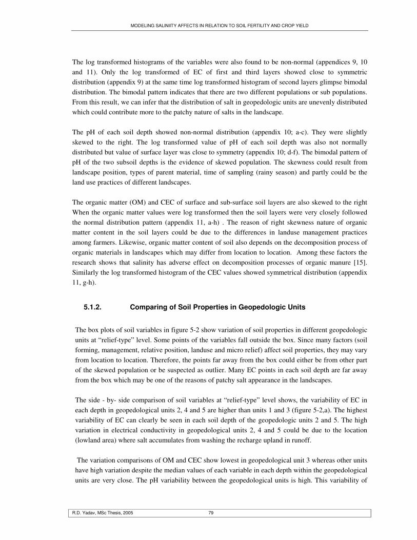
MODELING SALINIITY AFFECTS IN RELATION TO SOIL FERTILITY AND CROP YIELD
R.D. Yadav, MSc Thesis, 2005 79
The log transformed histograms of the variables were also found to be non-normal (appendices 9, 10 and 11). Only the log transformed of EC of first and third layers showed close to symmetric distribution (appendix 9) at the same time log transformed histogram of second layers glimpse bimodal distribution. The bimodal pattern indicates that there are two different populations or sub populations. From this result, we can infer that the distribution of salt in geopedologic units are unevenly distributed which could contribute more to the patchy nature of salts in the landscape. The pH of each soil depth showed non-normal distribution (appendix 10; a-c). They were slightly skewed to the right. The log transformed value of pH of each soil depth was also not normally distributed but value of surface layer was close to symmetry (appendix 10; d-f). The bimodal pattern of pH of the two subsoil depths is the evidence of skewed population. The skewness could result from landscape position, types of parent material, time of sampling (rainy season) and partly could be the land use practices of different landscapes. The organic matter (OM) and CEC of surface and sub-surface soil layers are also skewed to the right When the organic matter values were log transformed then the soil layers were very closely followed the normal distribution pattern (appendix 11, a-h) . The reason of right skewness nature of organic matter content in the soil layers could be due to the differences in landuse management practices among farmers. Likewise, organic matter content of soil also depends on the decomposition process of organic materials in landscapes which may differ from location to location. Among these factors the research shows that salinity has adverse effect on decomposition processes of organic manure [15]. Similarly the log transformed histogram of the CEC values showed symmetrical distribution (appendix 11, g-h).
5.1.2. Comparing of Soil Properties in Geopedologic Units
The box plots of soil variables in figure 5-2 show variation of soil properties in different geopedologic units at “relief-type” level. Some points of the variables fall outside the box. Since many factors (soil forming, management, relative position, landuse and micro relief) affect soil properties, they may vary from location to location. Therefore, the points far away from the box could either be from other part of the skewed population or be suspected as outlier. Many EC points in each soil depth are far away from the box which may be one of the reasons of patchy salt appearance in the landscapes. The side - by- side comparison of soil variables at “relief-type” level shows, the variability of EC in each depth in geopedological units 2, 4 and 5 are higher than units 1 and 3 (figure 5-2,a). The highest variability of EC can clearly be seen in each soil depth of the geopedologic units 2 and 5. The high variation in electrical conductivity in geopedological units 2, 4 and 5 could be due to the location (lowland area) where salt accumulates from washing the recharge upland in runoff. The variation comparisons of OM and CEC show lowest in geopedological unit 3 whereas other units have high variation despite the median values of each variable in each depth within the geopedological units are very close. The pH variability between the geopedological units is high. This variability of
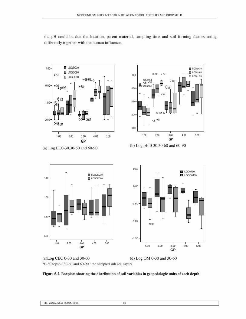
MODELING SALINIITY AFFECTS IN RELATION TO SOIL FERTILITY AND CROP YIELD
R.D. Yadav, MSc Thesis, 2005 80
the pH could be due the location, parent material, sampling time and soil forming factors acting differently together with the human influence.
1.00 2.00 3.00 4.00 5.00
GP
-2.00
-1.00
0.00
1.00
49
5413
958
18
26
67
26
51
68
5
51
68
51
68
LOGEC30LOGEC60LOGEC90
(a) Log EC0-30,30-60 and 60-90
1.00 2.00 3.00 4.00 5.00
GP
0.60
0.70
0.80
0.90
1.00
61
8
70
68615154
17
68
61
60
70
8
5154
17
LOGpH30LOGpH60LOGpH90
(b) Log pH 0-30,30-60 and 60-90
1.00 2.00 3.00 4.00 5.00
GP
0.00
0.50
1.00
1.50LOGCEC30LOGCEC60
(c)Log CEC 0-30 and 30-60
1.00 2.00 3.00 4.00 5.00
GP
-1.50
-1.00
-0.50
0.00
0.50
31
LGOM30LOGOM60
(d) Log OM 0-30 and 30-60 *0-30 topsoil,30-60 and 60-90 : the sampled sub soil layers Figure 5-2. Boxplots showing the distribution of soil variables in geopedologic units of each depth

MODELING SALINIITY AFFECTS IN RELATION TO SOIL FERTILITY AND CROP YIELD
R.D. Yadav, MSc Thesis, 2005 81
5.1.3. Variation of EC and pH, in Geopedologic Units
Analysis of variance (ANOVA) shows (table 5-1) the stratification significance which answer the research question related to one of the objective of the study. ANOVA test of EC and pH show significant result at “relief-type” level (p<0.05) in each soil depth (table 5-1). Therefore, the observed difference of salinity and pH of soil geopedologic units at “relief-type” level varies among the geopedological units in each soil depth (figure 5-3). Table 5-1: One way ANOVA of LogEC and Log pH
Variables Sum of Squares df Mean Square F Sig.
LOGEC30 Between Groups 5.794 4 1.449 4.160 .005
Within Groups 22.286 64 .348 LOGEC60 Between Groups 9.574 4 2.393 6.756 .000
Within Groups 22.674 64 0.354 LOGEC90 Between Groups 12.601 4 3.150 9.814 .000
Within Groups 20.545 64 0.321 LOGpH30 Between Groups 0.100 4 0.025 4.902 .002
Within Groups 0.320 63 0.005 LOGpH60 Between Groups 0.264 4 0.066 9.518 .000
Within Groups 0.437 63 0.007 LOGpH90 Between Groups 0.436 4 0.109 17.228 .000
Within Groups 0.399 63 0.006
0
0.3
0.6
0.9
Mean EC(dS/m)
Dep
th (
m)
Series2 1.42 1.42 1.47 1.73
Series1 0 30 60 90
1 2 3 4
0
0.3
0.6
0.9
pH
Dep
th(m
)
Series2 6.867477 6.867477 6.866729 6.989439
Series1 0 30 60 90
1 2 3 4
Figure 5-3. Changes of EC and pH with soil depth
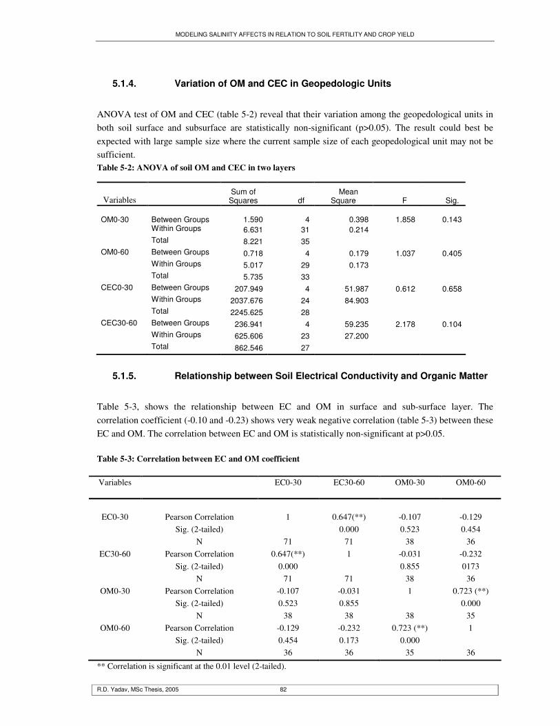
MODELING SALINIITY AFFECTS IN RELATION TO SOIL FERTILITY AND CROP YIELD
R.D. Yadav, MSc Thesis, 2005 82
5.1.4. Variation of OM and CEC in Geopedologic Units
ANOVA test of OM and CEC (table 5-2) reveal that their variation among the geopedological units in both soil surface and subsurface are statistically non-significant (p>0.05). The result could best be expected with large sample size where the current sample size of each geopedological unit may not be sufficient. Table 5-2: ANOVA of soil OM and CEC in two layers
Variables Sum of
Squares df Mean Square F Sig.
OM0-30
Between Groups
1.590
4
0.398
1.858
0.143
Within Groups 6.631 31 0.214 Total 8.221 35 OM0-60 Between Groups 0.718 4 0.179 1.037 0.405 Within Groups 5.017 29 0.173 Total 5.735 33 CEC0-30 Between Groups 207.949 4 51.987 0.612 0.658 Within Groups 2037.676 24 84.903 Total 2245.625 28 CEC30-60 Between Groups 236.941 4 59.235 2.178 0.104 Within Groups 625.606 23 27.200 Total 862.546 27
5.1.5. Relationship between Soil Electrical Conductivity and Organic Matter
Table 5-3, shows the relationship between EC and OM in surface and sub-surface layer. The correlation coefficient (-0.10 and -0.23) shows very weak negative correlation (table 5-3) between these EC and OM. The correlation between EC and OM is statistically non-significant at p>0.05. Table 5-3: Correlation between EC and OM coefficient
Variables EC0-30 EC30-60 OM0-30 OM0-60
EC0-30
Pearson Correlation
1
0.647(**)
-0.107
-0.129
Sig. (2-tailed) 0.000 0.523 0.454 N 71 71 38 36
EC30-60 Pearson Correlation 0.647(**) 1 -0.031 -0.232 Sig. (2-tailed) 0.000 0.855 0173 N 71 71 38 36
OM0-30 Pearson Correlation -0.107 -0.031 1 0.723 (**) Sig. (2-tailed) 0.523 0.855 0.000 N 38 38 38 35
OM0-60 Pearson Correlation -0.129 -0.232 0.723 (**) 1 Sig. (2-tailed) 0.454 0.173 0.000 N 36 36 35 36
** Correlation is significant at the 0.01 level (2-tailed).
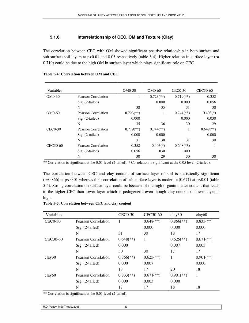
MODELING SALINIITY AFFECTS IN RELATION TO SOIL FERTILITY AND CROP YIELD
R.D. Yadav, MSc Thesis, 2005 83
5.1.6. Interrelationship of CEC, OM and Texture (Clay)
The correlation between CEC with OM showed significant positive relationship in both surface and sub-surface soil layers at p<0.01 and 0.05 respectively (table 5-4). Higher relation in surface layer (r= 0.719) could be due to the high OM in surface layer which plays significant role on CEC. Table 5-4: Correlation between OM and CEC
Variables OM0-30 OM0-60 CEC0-30
CEC30-60
OM0-30 Pearson Correlation 1 0.723(**) 0.719(**) 0.352 Sig. (2-tailed) 0.000 0.000 0.056 N 38 35 31 30 OM0-60 Pearson Correlation 0.723(**) 1 0.744(**) 0.403(*) Sig. (2-tailed) 0.000 0.000 0.030 N 35 36 30 29 CEC0-30 Pearson Correlation 0.719(**) 0.744(**) 1 0.648(**) Sig. (2-tailed) 0.000 0.000 0.000 N 31 30 31 30 CEC30-60 Pearson Correlation 0.352 0.403(*) 0.648(**) 1 Sig. (2-tailed) 0.056 .030 .000 N 30 29 30 30
** Correlation is significant at the 0.01 level (2-tailed). * Correlation is significant at the 0.05 level (2-tailed).
The correlation between CEC and clay content of surface layer of soil is statistically significant (r=0.866) at p< 0.01 whereas their correlation of sub-surface layer is moderate (0.671) at p<0.01 (table 5-5). Strong correlation on surface layer could be because of the high organic matter content that leads to the higher CEC than lower layer which is pedogenetic even though clay content of lower layer is high. Table 5-5: Correlation between CEC and clay content
Variables CEC0-30 CEC30-60 clay30 clay60
CEC0-30 Pearson Correlation 1 0.648(**) 0.866(**) 0.833(**) Sig. (2-tailed) 0.000 0.000 0.000 N 31 30 18 17 CEC30-60 Pearson Correlation 0.648(**) 1 0.625(**) 0.671(**) Sig. (2-tailed) 0.000 0.007 0.003 N 30 30 17 17 clay30 Pearson Correlation 0.866(**) 0.625(**) 1 0.901(**) Sig. (2-tailed) 0.000 0.007 0.000 N 18 17 20 18 clay60 Pearson Correlation 0.833(**) 0.671(**) 0.901(**) 1 Sig. (2-tailed) 0.000 0.003 0.000 N 17 17 18 18
** Correlation is significant at the 0.01 level (2-tailed).
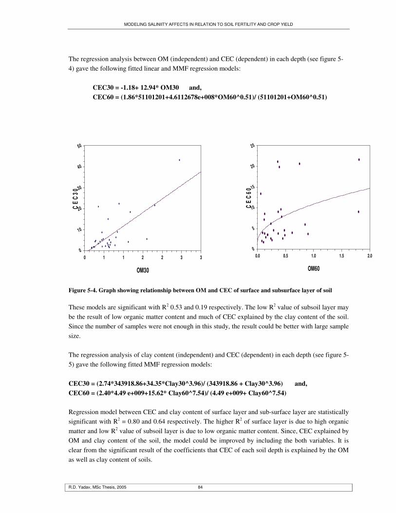
MODELING SALINIITY AFFECTS IN RELATION TO SOIL FERTILITY AND CROP YIELD
R.D. Yadav, MSc Thesis, 2005 84
The regression analysis between OM (independent) and CEC (dependent) in each depth (see figure 5-4) gave the following fitted linear and MMF regression models: CEC30 = -1.18+ 12.94* OM30 and, CEC60 = (1.86*51101201+4.6112678e+008*OM60^0.51)/ (51101201+OM60^0.51)
OM30
CE
C30
0 1 1 2 2 3 30
10
20
30
40
50
OM60
CE
C60
0.0 0.5 1.0 1.5 2.00
5
10
15
20
25
Figure 5-4. Graph showing relationship between OM and CEC of surface and subsurface layer of soil These models are significant with R2 0.53 and 0.19 respectively. The low R2 value of subsoil layer may be the result of low organic matter content and much of CEC explained by the clay content of the soil. Since the number of samples were not enough in this study, the result could be better with large sample size. The regression analysis of clay content (independent) and CEC (dependent) in each depth (see figure 5-5) gave the following fitted MMF regression models: CEC30 = (2.74*343918.86+34.35*Clay30^3.96)/ (343918.86 + Clay30^3.96) and, CEC60 = (2.40*4.49 e+009+15.62* Clay60^7.54)/ (4.49 e+009+ Clay60^7.54) Regression model between CEC and clay content of surface layer and sub-surface layer are statistically significant with R2 = 0.80 and 0.64 respectively. The higher R2 of surface layer is due to high organic matter and low R2 value of subsoil layer is due to low organic matter content. Since, CEC explained by OM and clay content of the soil, the model could be improved by including the both variables. It is clear from the significant result of the coefficients that CEC of each soil depth is explained by the OM as well as clay content of soils.
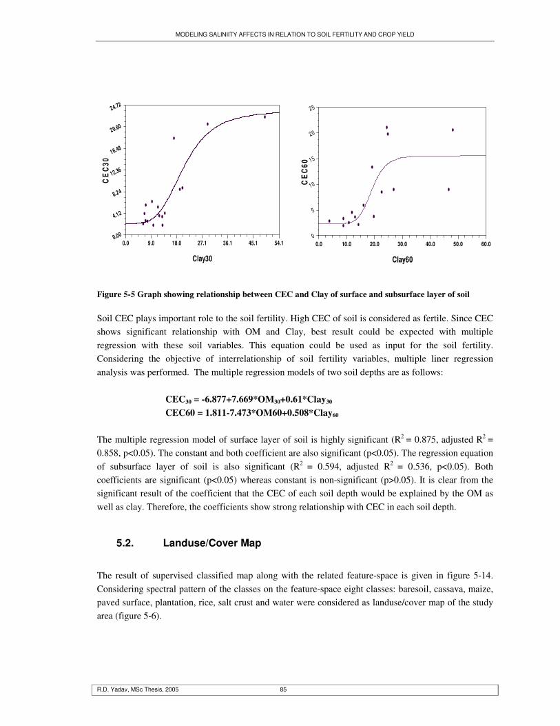
MODELING SALINIITY AFFECTS IN RELATION TO SOIL FERTILITY AND CROP YIELD
R.D. Yadav, MSc Thesis, 2005 85
Clay30
CE
C30
0.0 9.0 18.0 27.1 36.1 45.1 54.10.00
4.12
8.24
12.36
16.48
20.60
24.72
Clay60
CE
C60
0.0 10.0 20.0 30.0 40.0 50.0 60.00
5
10
15
20
25
Figure 5-5 Graph showing relationship between CEC and Clay of surface and subsurface layer of soil Soil CEC plays important role to the soil fertility. High CEC of soil is considered as fertile. Since CEC shows significant relationship with OM and Clay, best result could be expected with multiple regression with these soil variables. This equation could be used as input for the soil fertility. Considering the objective of interrelationship of soil fertility variables, multiple liner regression analysis was performed. The multiple regression models of two soil depths are as follows:
CEC30 = -6.877+7.669*OM30+0.61*Clay30 CEC60 = 1.811-7.473*OM60+0.508*Clay60
The multiple regression model of surface layer of soil is highly significant (R2 = 0.875, adjusted R2 = 0.858, p<0.05). The constant and both coefficient are also significant (p<0.05). The regression equation of subsurface layer of soil is also significant (R2 = 0.594, adjusted R2 = 0.536, p<0.05). Both coefficients are significant (p<0.05) whereas constant is non-significant (p>0.05). It is clear from the significant result of the coefficient that the CEC of each soil depth would be explained by the OM as well as clay. Therefore, the coefficients show strong relationship with CEC in each soil depth.
5.2. Landuse/Cover Map
The result of supervised classified map along with the related feature-space is given in figure 5-14. Considering spectral pattern of the classes on the feature-space eight classes: baresoil, cassava, maize, paved surface, plantation, rice, salt crust and water were considered as landuse/cover map of the study area (figure 5-6).
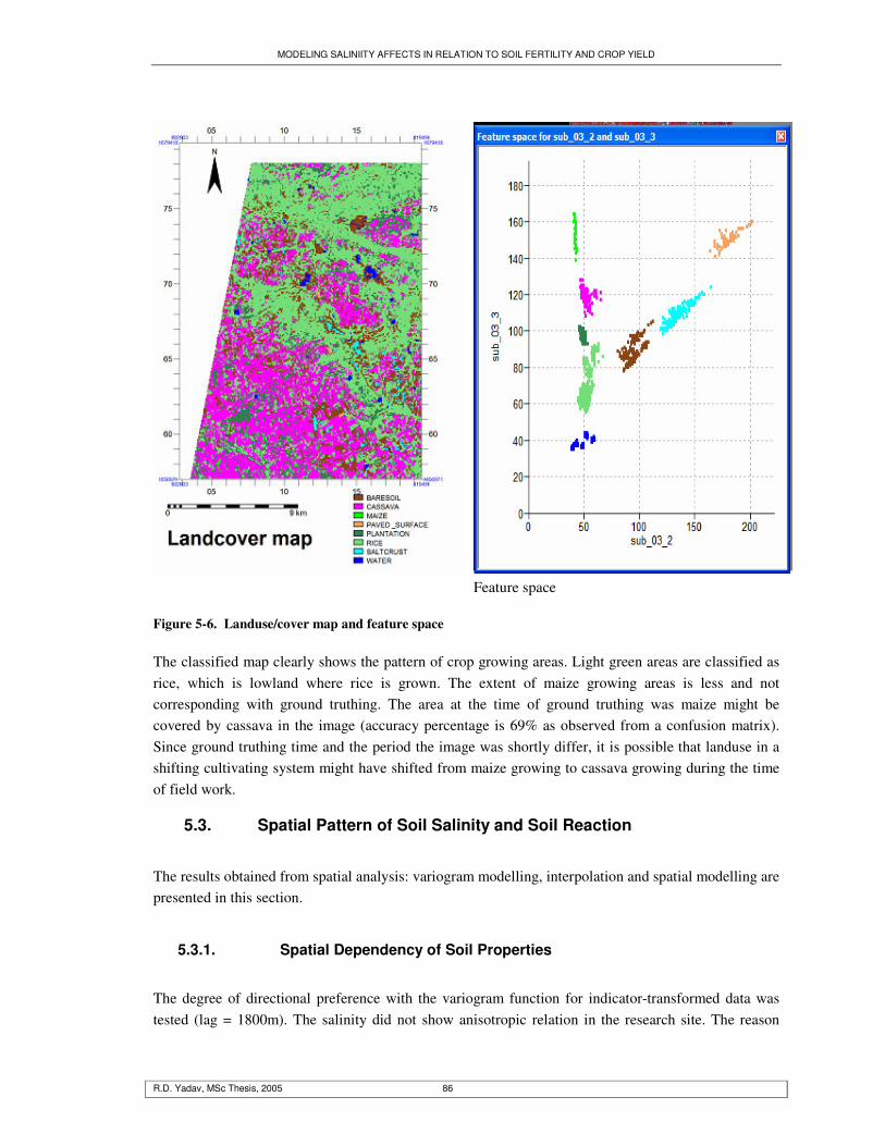
MODELING SALINIITY AFFECTS IN RELATION TO SOIL FERTILITY AND CROP YIELD
R.D. Yadav, MSc Thesis, 2005 86
Feature space
Figure 5-6. Landuse/cover map and feature space The classified map clearly shows the pattern of crop growing areas. Light green areas are classified as rice, which is lowland where rice is grown. The extent of maize growing areas is less and not corresponding with ground truthing. The area at the time of ground truthing was maize might be covered by cassava in the image (accuracy percentage is 69% as observed from a confusion matrix). Since ground truthing time and the period the image was shortly differ, it is possible that landuse in a shifting cultivating system might have shifted from maize growing to cassava growing during the time of field work.
5.3. Spatial Pattern of Soil Salinity and Soil Reaction
The results obtained from spatial analysis: variogram modelling, interpolation and spatial modelling are presented in this section.
5.3.1. Spatial Dependency of Soil Properties
The degree of directional preference with the variogram function for indicator-transformed data was tested (lag = 1800m). The salinity did not show anisotropic relation in the research site. The reason
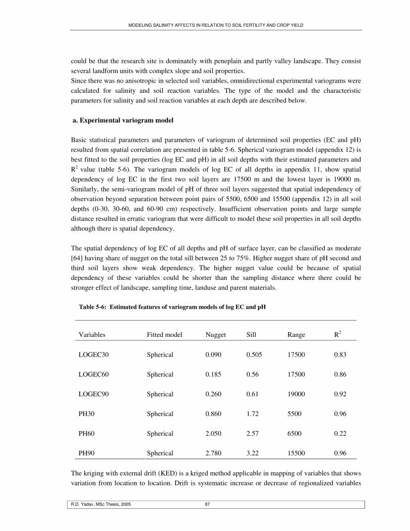
MODELING SALINIITY AFFECTS IN RELATION TO SOIL FERTILITY AND CROP YIELD
R.D. Yadav, MSc Thesis, 2005 87
could be that the research site is dominately with peneplain and partly valley landscape. They consist several landform units with complex slope and soil properties. Since there was no anisotropic in selected soil variables, omnidirectional experimental variograms were calculated for salinity and soil reaction variables. The type of the model and the characteristic parameters for salinity and soil reaction variables at each depth are described below. a. Experimental variogram model Basic statistical parameters and parameters of variogram of determined soil properties (EC and pH) resulted from spatial correlation are presented in table 5-6. Spherical variogram model (appendix 12) is best fitted to the soil properties (log EC and pH) in all soil depths with their estimated parameters and R2 value (table 5-6). The variogram models of log EC of all depths in appendix 11, show spatial dependency of log EC in the first two soil layers are 17500 m and the lowest layer is 19000 m. Similarly, the semi-variogram model of pH of three soil layers suggested that spatial independency of observation beyond separation between point pairs of 5500, 6500 and 15500 (appendix 12) in all soil depths (0-30, 30-60, and 60-90 cm) respectively. Insufficient observation points and large sample distance resulted in erratic variogram that were difficult to model these soil properties in all soil depths although there is spatial dependency. The spatial dependency of log EC of all depths and pH of surface layer, can be classified as moderate [64] having share of nugget on the total sill between 25 to 75%. Higher nugget share of pH second and third soil layers show weak dependency. The higher nugget value could be because of spatial dependency of these variables could be shorter than the sampling distance where there could be stronger effect of landscape, sampling time, landuse and parent materials. Table 5-6: Estimated features of variogram models of log EC and pH
Variables Fitted model Nugget Sill Range R2
LOGEC30 Spherical 0.090 0.505 17500 0.83 LOGEC60 Spherical 0.185 0.56 17500 0.86 LOGEC90 Spherical 0.260 0.61 19000 0.92 PH30 Spherical 0.860 1.72 5500 0.96 PH60 Spherical 2.050 2.57 6500 0.22 PH90 Spherical 2.780 3.22 15500 0.96
The kriging with external drift (KED) is a kriged method applicable in mapping of variables that shows variation from location to location. Drift is systematic increase or decrease of regionalized variables
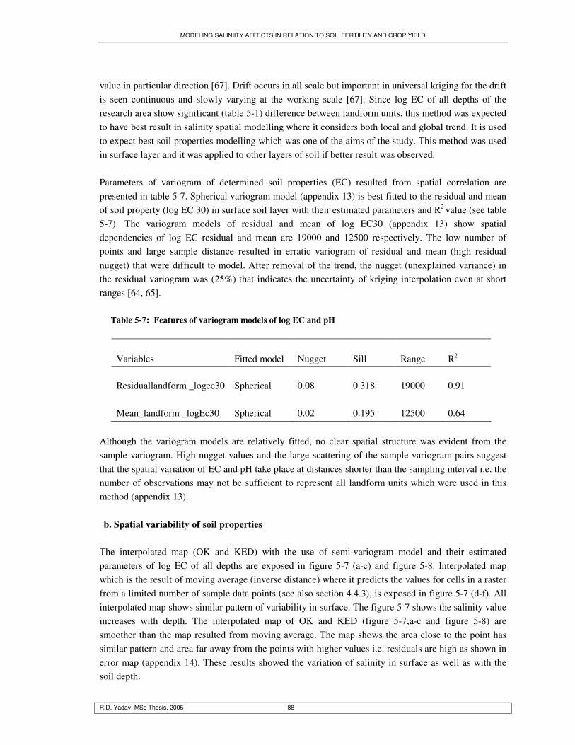
MODELING SALINIITY AFFECTS IN RELATION TO SOIL FERTILITY AND CROP YIELD
R.D. Yadav, MSc Thesis, 2005 88
value in particular direction [67]. Drift occurs in all scale but important in universal kriging for the drift is seen continuous and slowly varying at the working scale [67]. Since log EC of all depths of the research area show significant (table 5-1) difference between landform units, this method was expected to have best result in salinity spatial modelling where it considers both local and global trend. It is used to expect best soil properties modelling which was one of the aims of the study. This method was used in surface layer and it was applied to other layers of soil if better result was observed. Parameters of variogram of determined soil properties (EC) resulted from spatial correlation are presented in table 5-7. Spherical variogram model (appendix 13) is best fitted to the residual and mean of soil property (log EC 30) in surface soil layer with their estimated parameters and R2 value (see table 5-7). The variogram models of residual and mean of log EC30 (appendix 13) show spatial dependencies of log EC residual and mean are 19000 and 12500 respectively. The low number of points and large sample distance resulted in erratic variogram of residual and mean (high residual nugget) that were difficult to model. After removal of the trend, the nugget (unexplained variance) in the residual variogram was (25%) that indicates the uncertainty of kriging interpolation even at short ranges [64, 65]. Table 5-7: Features of variogram models of log EC and pH
Variables Fitted model Nugget Sill Range R2
Residuallandform _logec30 Spherical 0.08 0.318 19000 0.91
Mean_landform _logEc30 Spherical
0.02
0.195
12500
0.64
Although the variogram models are relatively fitted, no clear spatial structure was evident from the sample variogram. High nugget values and the large scattering of the sample variogram pairs suggest that the spatial variation of EC and pH take place at distances shorter than the sampling interval i.e. the number of observations may not be sufficient to represent all landform units which were used in this method (appendix 13). b. Spatial variability of soil properties
The interpolated map (OK and KED) with the use of semi-variogram model and their estimated parameters of log EC of all depths are exposed in figure 5-7 (a-c) and figure 5-8. Interpolated map which is the result of moving average (inverse distance) where it predicts the values for cells in a raster from a limited number of sample data points (see also section 4.4.3), is exposed in figure 5-7 (d-f). All interpolated map shows similar pattern of variability in surface. The figure 5-7 shows the salinity value increases with depth. The interpolated map of OK and KED (figure 5-7;a-c and figure 5-8) are smoother than the map resulted from moving average. The map shows the area close to the point has similar pattern and area far away from the points with higher values i.e. residuals are high as shown in error map (appendix 14). These results showed the variation of salinity in surface as well as with the soil depth.

MODELING SALINIITY AFFECTS IN RELATION TO SOIL FERTILITY AND CROP YIELD
R.D. Yadav, MSc Thesis, 2005 89
(a)Log EC30 map from OK (b)Log EC60 map from OK
(c)Log EC90 map from OK
(d)Log EC30 map of MAV
(e)Log EC60 map of MAV
(f)Log EC90 map of MAV
Figure 5-7. Interpolation map of log EC of three layers from Ordinary Kriging (OK) and moving average (MAV)
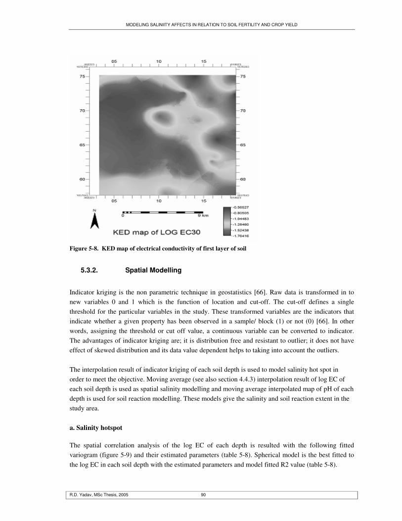
MODELING SALINIITY AFFECTS IN RELATION TO SOIL FERTILITY AND CROP YIELD
R.D. Yadav, MSc Thesis, 2005 90
Figure 5-8. KED map of electrical conductivity of first layer of soil
5.3.2. Spatial Modelling
Indicator kriging is the non parametric technique in geostatistics [66]. Raw data is transformed in to new variables 0 and 1 which is the function of location and cut-off. The cut-off defines a single threshold for the particular variables in the study. These transformed variables are the indicators that indicate whether a given property has been observed in a sample/ block (1) or not (0) [66]. In other words, assigning the threshold or cut off value, a continuous variable can be converted to indicator. The advantages of indicator kriging are; it is distribution free and resistant to outlier; it does not have effect of skewed distribution and its data value dependent helps to taking into account the outliers. The interpolation result of indicator kriging of each soil depth is used to model salinity hot spot in order to meet the objective. Moving average (see also section 4.4.3) interpolation result of log EC of each soil depth is used as spatial salinity modelling and moving average interpolated map of pH of each depth is used for soil reaction modelling. These models give the salinity and soil reaction extent in the study area. a. Salinity hotspot The spatial correlation analysis of the log EC of each depth is resulted with the following fitted variogram (figure 5-9) and their estimated parameters (table 5-8). Spherical model is the best fitted to the log EC in each soil depth with the estimated parameters and model fitted R2 value (table 5-8).
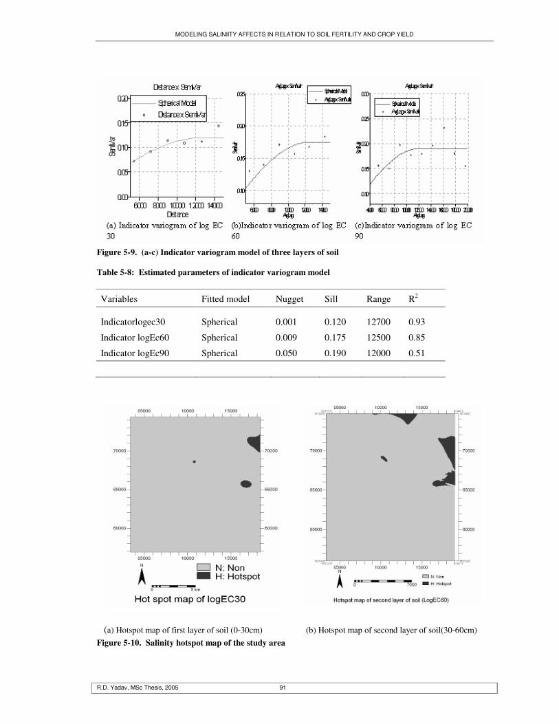
MODELING SALINIITY AFFECTS IN RELATION TO SOIL FERTILITY AND CROP YIELD
R.D. Yadav, MSc Thesis, 2005 91
Figure 5-9. (a-c) Indicator variogram model of three layers of soil Table 5-8: Estimated parameters of indicator variogram model
Variables Fitted model Nugget Sill Range R2
Indicatorlogec30 Spherical 0.001 0.120 12700 0.93
Indicator logEc60 Spherical 0.009 0.175 12500 0.85
Indicator logEc90 Spherical 0.050 0.190 12000 0.51
(a) Hotspot map of first layer of soil (0-30cm) (b) Hotspot map of second layer of soil(30-60cm) Figure 5-10. Salinity hotspot map of the study area

MODELING SALINIITY AFFECTS IN RELATION TO SOIL FERTILITY AND CROP YIELD
R.D. Yadav, MSc Thesis, 2005 92
The dark areas on both maps (533.5 ha in surface layers and 1273.75 ha in subsurface layer) are the indication of salinity hotspot. The hotspot area is having 80 or more percent probability of crop failure due to high soil salinity. The hotspot area in sub-surface soil layer is highest among the three depths. It is probably the salt might have accumulated to the sub-surface soil layer where sample was collected in rainy season. The soil depth 60 to 90 cm does not show hotspot. It could be the erratic nature of salt which has spatial dependency less than the sampling design followed. b. Salinity and soil reaction The spatial distribution of electrical conductivity shows significant variation at all three soil depths. The salinity extent increases with depth. It is apparent and not a surprising result where soil sampling was done in rainy season, as in this case salt moves down to lower parts of the soil profile.
(a)Salinity map of top 30 cm (b) Salinity map of 30-60 cm (c) Salinity map of top 60-90 cm Figure 5-11. Salinity map of different layers of soil of the study area
The areas of salt affected surface layer, moderate, strongly and extremely-saline are 192 ha, 34 ha and 9 ha respectively. The extent in the sub-surface layer (30- 60 cm) are 534 ha, 62 ha and 3 ha under moderately, strongly and extremely saline, respectively. Similarly the extent has become 995, 216 and 11 ha respectively under the same categories as surface and subsurface layer of the soil. The low laying area clearly shows the highest salinity. The highly salinity areas in the figure 5-11 correspond partly with the lateral vale, glacis and flood plain. The salinity extent is increased with depth and the area of surface layer which are not saline now has the chance to be saline during the dry period because of capillary rise from the lower layers. Another reason could be the runoff water during the monsoon which washes up the salt from the upland transferred to and collected in the lowland. Water in dry period is evaporated leaving salt behind in the soil.
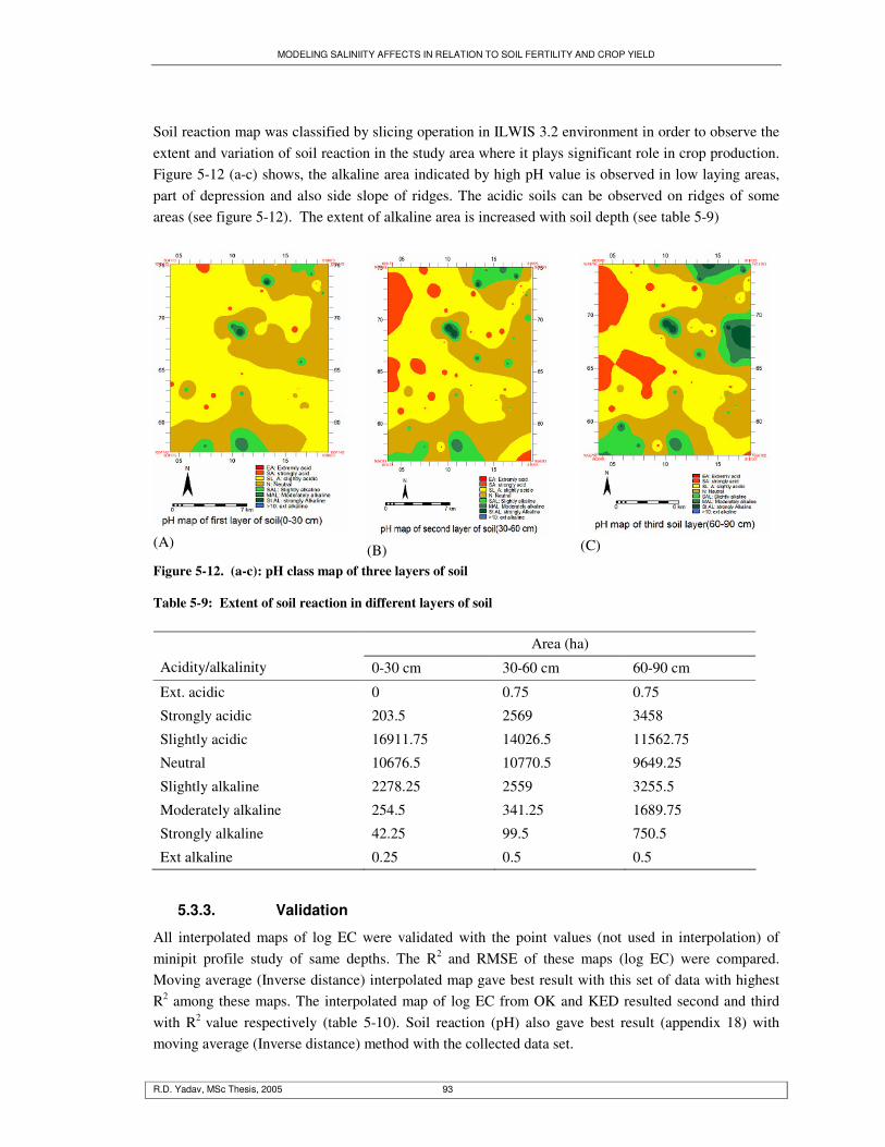
MODELING SALINIITY AFFECTS IN RELATION TO SOIL FERTILITY AND CROP YIELD
R.D. Yadav, MSc Thesis, 2005 93
Soil reaction map was classified by slicing operation in ILWIS 3.2 environment in order to observe the extent and variation of soil reaction in the study area where it plays significant role in crop production. Figure 5-12 (a-c) shows, the alkaline area indicated by high pH value is observed in low laying areas, part of depression and also side slope of ridges. The acidic soils can be observed on ridges of some areas (see figure 5-12). The extent of alkaline area is increased with soil depth (see table 5-9)
(A)
(B)
(C)
Figure 5-12. (a-c): pH class map of three layers of soil Table 5-9: Extent of soil reaction in different layers of soil
Area (ha)
Acidity/alkalinity 0-30 cm 30-60 cm 60-90 cm
Ext. acidic 0 0.75 0.75
Strongly acidic 203.5 2569 3458
Slightly acidic 16911.75 14026.5 11562.75
Neutral 10676.5 10770.5 9649.25
Slightly alkaline 2278.25 2559 3255.5
Moderately alkaline 254.5 341.25 1689.75
Strongly alkaline 42.25 99.5 750.5
Ext alkaline 0.25 0.5 0.5
5.3.3. Validation
All interpolated maps of log EC were validated with the point values (not used in interpolation) of minipit profile study of same depths. The R2 and RMSE of these maps (log EC) were compared. Moving average (Inverse distance) interpolated map gave best result with this set of data with highest R2 among these maps. The interpolated map of log EC from OK and KED resulted second and third with R2 value respectively (table 5-10). Soil reaction (pH) also gave best result (appendix 18) with moving average (Inverse distance) method with the collected data set.
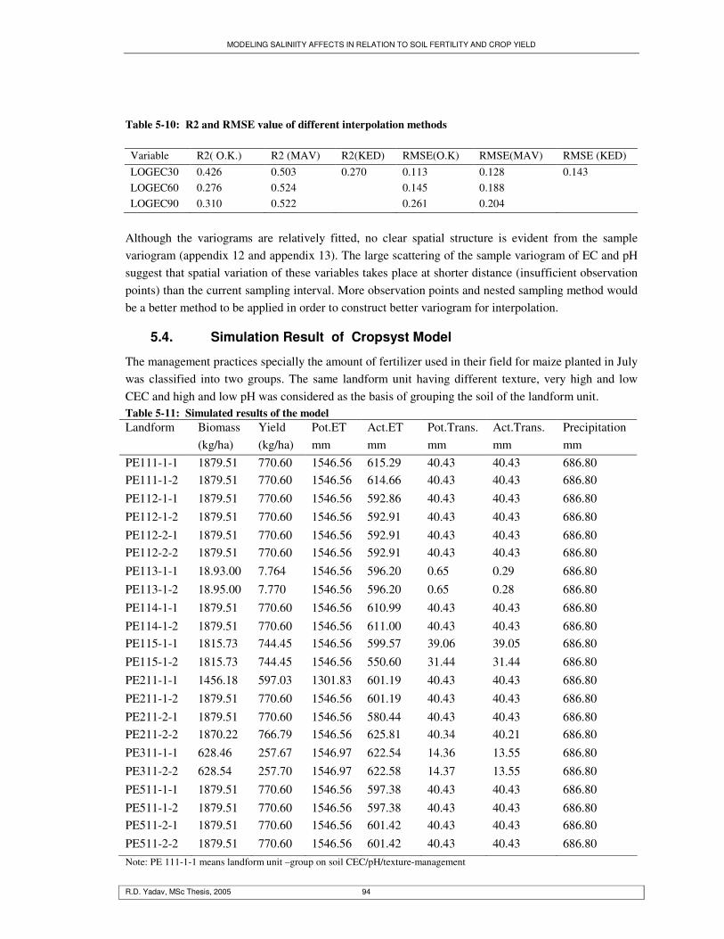
MODELING SALINIITY AFFECTS IN RELATION TO SOIL FERTILITY AND CROP YIELD
R.D. Yadav, MSc Thesis, 2005 94
Table 5-10: R2 and RMSE value of different interpolation methods Variable R2( O.K.) R2 (MAV) R2(KED) RMSE(O.K) RMSE(MAV) RMSE (KED) LOGEC30 0.426 0.503 0.270 0.113 0.128 0.143 LOGEC60 0.276 0.524 0.145 0.188 LOGEC90 0.310 0.522 0.261 0.204
Although the variograms are relatively fitted, no clear spatial structure is evident from the sample variogram (appendix 12 and appendix 13). The large scattering of the sample variogram of EC and pH suggest that spatial variation of these variables takes place at shorter distance (insufficient observation points) than the current sampling interval. More observation points and nested sampling method would be a better method to be applied in order to construct better variogram for interpolation.
5.4. Simulation Result of Cropsyst Model
The management practices specially the amount of fertilizer used in their field for maize planted in July was classified into two groups. The same landform unit having different texture, very high and low CEC and high and low pH was considered as the basis of grouping the soil of the landform unit. Table 5-11: Simulated results of the model Landform Biomass
(kg/ha) Yield (kg/ha)
Pot.ET mm
Act.ET mm
Pot.Trans. mm
Act.Trans. mm
Precipitation mm
PE111-1-1 1879.51 770.60 1546.56 615.29 40.43 40.43 686.80 PE111-1-2 1879.51 770.60 1546.56 614.66 40.43 40.43 686.80 PE112-1-1 1879.51 770.60 1546.56 592.86 40.43 40.43 686.80 PE112-1-2 1879.51 770.60 1546.56 592.91 40.43 40.43 686.80 PE112-2-1 1879.51 770.60 1546.56 592.91 40.43 40.43 686.80 PE112-2-2 1879.51 770.60 1546.56 592.91 40.43 40.43 686.80 PE113-1-1 18.93.00 7.764 1546.56 596.20 0.65 0.29 686.80 PE113-1-2 18.95.00 7.770 1546.56 596.20 0.65 0.28 686.80 PE114-1-1 1879.51 770.60 1546.56 610.99 40.43 40.43 686.80 PE114-1-2 1879.51 770.60 1546.56 611.00 40.43 40.43 686.80 PE115-1-1 1815.73 744.45 1546.56 599.57 39.06 39.05 686.80 PE115-1-2 1815.73 744.45 1546.56 550.60 31.44 31.44 686.80 PE211-1-1 1456.18 597.03 1301.83 601.19 40.43 40.43 686.80 PE211-1-2 1879.51 770.60 1546.56 601.19 40.43 40.43 686.80 PE211-2-1 1879.51 770.60 1546.56 580.44 40.43 40.43 686.80 PE211-2-2 1870.22 766.79 1546.56 625.81 40.34 40.21 686.80 PE311-1-1 628.46 257.67 1546.97 622.54 14.36 13.55 686.80 PE311-2-2 628.54 257.70 1546.97 622.58 14.37 13.55 686.80 PE511-1-1 1879.51 770.60 1546.56 597.38 40.43 40.43 686.80 PE511-1-2 1879.51 770.60 1546.56 597.38 40.43 40.43 686.80 PE511-2-1 1879.51 770.60 1546.56 601.42 40.43 40.43 686.80 PE511-2-2 1879.51 770.60 1546.56 601.42 40.43 40.43 686.80 Note: PE 111-1-1 means landform unit –group on soil CEC/pH/texture-management
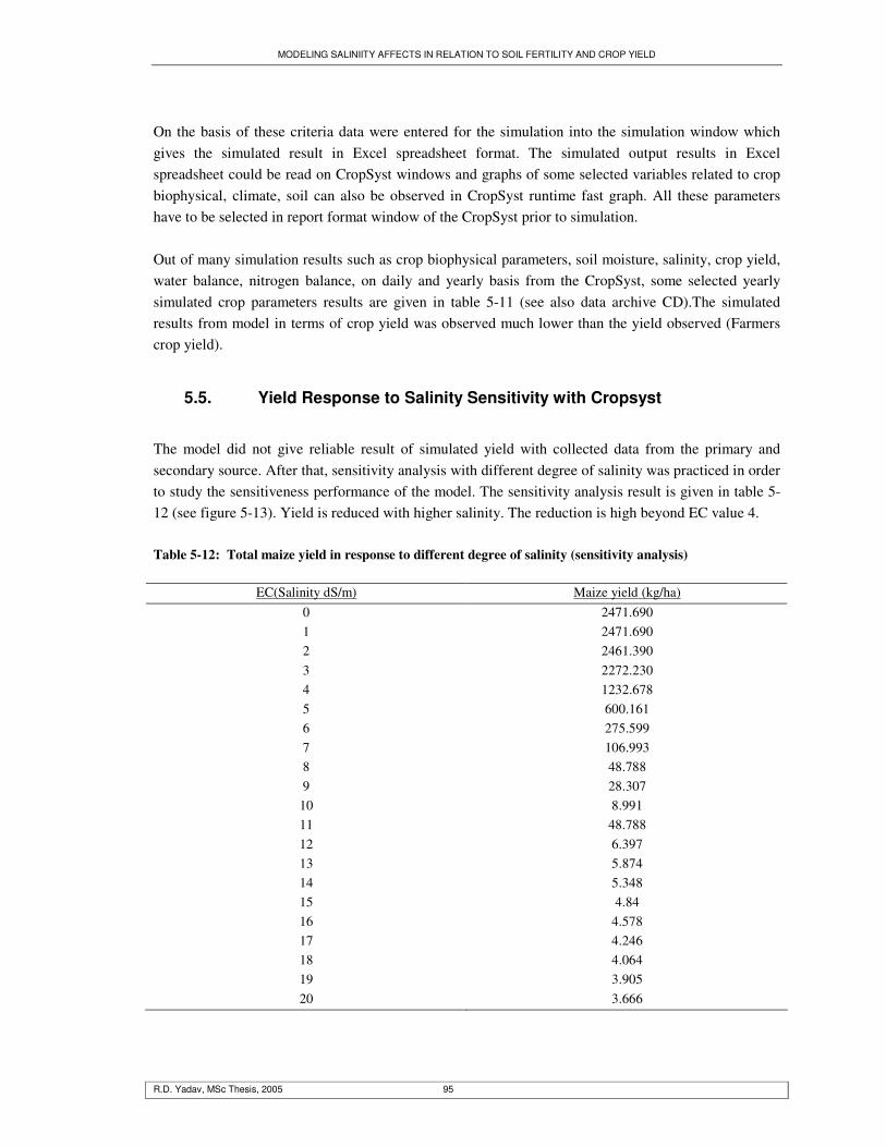
MODELING SALINIITY AFFECTS IN RELATION TO SOIL FERTILITY AND CROP YIELD
R.D. Yadav, MSc Thesis, 2005 95
On the basis of these criteria data were entered for the simulation into the simulation window which gives the simulated result in Excel spreadsheet format. The simulated output results in Excel spreadsheet could be read on CropSyst windows and graphs of some selected variables related to crop biophysical, climate, soil can also be observed in CropSyst runtime fast graph. All these parameters have to be selected in report format window of the CropSyst prior to simulation. Out of many simulation results such as crop biophysical parameters, soil moisture, salinity, crop yield, water balance, nitrogen balance, on daily and yearly basis from the CropSyst, some selected yearly simulated crop parameters results are given in table 5-11 (see also data archive CD).The simulated results from model in terms of crop yield was observed much lower than the yield observed (Farmers crop yield).
5.5. Yield Response to Salinity Sensitivity with Cropsyst
The model did not give reliable result of simulated yield with collected data from the primary and secondary source. After that, sensitivity analysis with different degree of salinity was practiced in order to study the sensitiveness performance of the model. The sensitivity analysis result is given in table 5-12 (see figure 5-13). Yield is reduced with higher salinity. The reduction is high beyond EC value 4. Table 5-12: Total maize yield in response to different degree of salinity (sensitivity analysis)
EC(Salinity dS/m) Maize yield (kg/ha) 0 2471.690 1 2471.690 2 2461.390 3 2272.230 4 1232.678 5 600.161 6 275.599 7 106.993 8 48.788 9 28.307 10 8.991 11 48.788 12 6.397 13 5.874 14 5.348 15 4.84 16 4.578 17 4.246 18 4.064 19 3.905 20 3.666
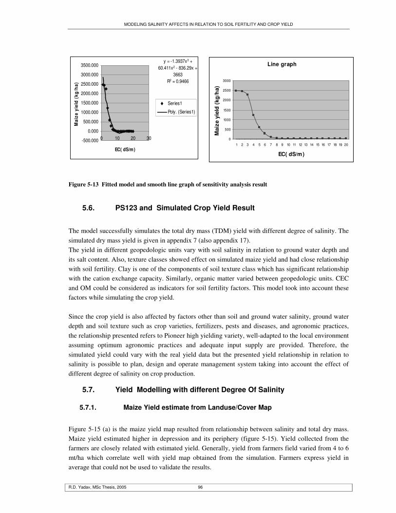
MODELING SALINIITY AFFECTS IN RELATION TO SOIL FERTILITY AND CROP YIELD
R.D. Yadav, MSc Thesis, 2005 96
y = -1.3937x3 + 60.411x2 - 836.29x +
3663R2 = 0.9466
-500.000
0.000
500.000
1000.000
1500.000
2000.000
2500.000
3000.000
3500.000
0 10 20 30
EC( dS/m)
Mai
ze y
ield
(kg
/ha)
Series1
Poly. (Series1)
Line graph
0
500
1000
1500
2000
2500
3000
1 2 3 4 5 6 7 8 9 10 11 12 13 14 15 16 17 18 19 20
EC( dS/m)
Mai
ze y
ield
(kg
/ha)
Figure 5-13 Fitted model and smooth line graph of sensitivity analysis result
5.6. PS123 and Simulated Crop Yield Result
The model successfully simulates the total dry mass (TDM) yield with different degree of salinity. The simulated dry mass yield is given in appendix 7 (also appendix 17). The yield in different geopedologic units vary with soil salinity in relation to ground water depth and its salt content. Also, texture classes showed effect on simulated maize yield and had close relationship with soil fertility. Clay is one of the components of soil texture class which has significant relationship with the cation exchange capacity. Similarly, organic matter varied between geopedologic units. CEC and OM could be considered as indicators for soil fertility factors. This model took into account these factors while simulating the crop yield. Since the crop yield is also affected by factors other than soil and ground water salinity, ground water depth and soil texture such as crop varieties, fertilizers, pests and diseases, and agronomic practices, the relationship presented refers to Pioneer high yielding variety, well-adapted to the local environment assuming optimum agronomic practices and adequate input supply are provided. Therefore, the simulated yield could vary with the real yield data but the presented yield relationship in relation to salinity is possible to plan, design and operate management system taking into account the effect of different degree of salinity on crop production.
5.7. Yield Modelling with different Degree Of Salinity
5.7.1. Maize Yield estimate from Landuse/Cover Map
Figure 5-15 (a) is the maize yield map resulted from relationship between salinity and total dry mass. Maize yield estimated higher in depression and its periphery (figure 5-15). Yield collected from the farmers are closely related with estimated yield. Generally, yield from farmers field varied from 4 to 6 mt/ha which correlate well with yield map obtained from the simulation. Farmers express yield in average that could not be used to validate the results.
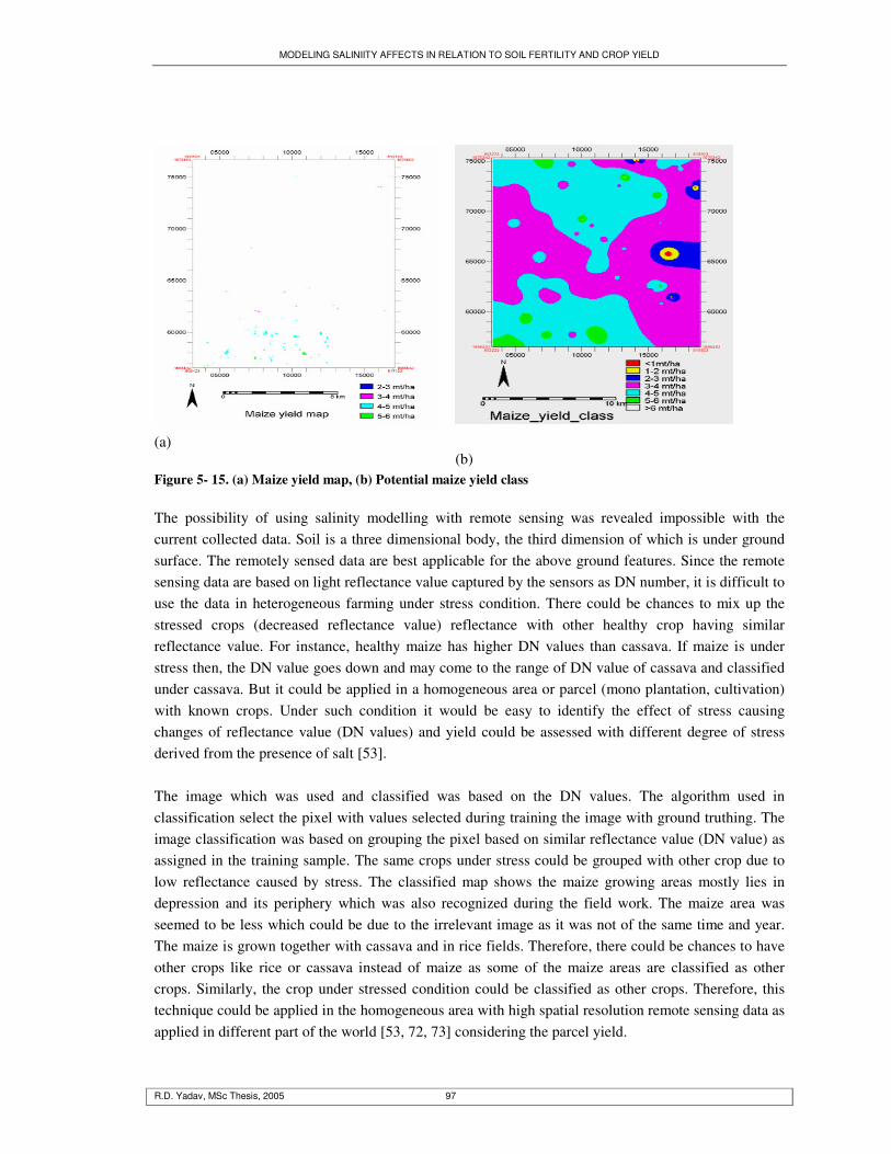
MODELING SALINIITY AFFECTS IN RELATION TO SOIL FERTILITY AND CROP YIELD
R.D. Yadav, MSc Thesis, 2005 97
(a)
(b)
Figure 5- 15. (a) Maize yield map, (b) Potential maize yield class The possibility of using salinity modelling with remote sensing was revealed impossible with the current collected data. Soil is a three dimensional body, the third dimension of which is under ground surface. The remotely sensed data are best applicable for the above ground features. Since the remote sensing data are based on light reflectance value captured by the sensors as DN number, it is difficult to use the data in heterogeneous farming under stress condition. There could be chances to mix up the stressed crops (decreased reflectance value) reflectance with other healthy crop having similar reflectance value. For instance, healthy maize has higher DN values than cassava. If maize is under stress then, the DN value goes down and may come to the range of DN value of cassava and classified under cassava. But it could be applied in a homogeneous area or parcel (mono plantation, cultivation) with known crops. Under such condition it would be easy to identify the effect of stress causing changes of reflectance value (DN values) and yield could be assessed with different degree of stress derived from the presence of salt [53]. The image which was used and classified was based on the DN values. The algorithm used in classification select the pixel with values selected during training the image with ground truthing. The image classification was based on grouping the pixel based on similar reflectance value (DN value) as assigned in the training sample. The same crops under stress could be grouped with other crop due to low reflectance caused by stress. The classified map shows the maize growing areas mostly lies in depression and its periphery which was also recognized during the field work. The maize area was seemed to be less which could be due to the irrelevant image as it was not of the same time and year. The maize is grown together with cassava and in rice fields. Therefore, there could be chances to have other crops like rice or cassava instead of maize as some of the maize areas are classified as other crops. Similarly, the crop under stressed condition could be classified as other crops. Therefore, this technique could be applied in the homogeneous area with high spatial resolution remote sensing data as applied in different part of the world [53, 72, 73] considering the parcel yield.

MODELING SALINIITY AFFECTS IN RELATION TO SOIL FERTILITY AND CROP YIELD
R.D. Yadav, MSc Thesis, 2005 98
5.7.2. Mathematical (Regression) Model for Crop Yield Estimation
The relationship between soil chemical properties, ground water properties and maize yield resulted the following significant (R2= 0.795 and adjusted R2=0.778) mathematical yield model (see appendix 8). The equation could be applied to estimate maize yield. MY = 5294.088-323.862 WEC-4.265 GWD – 41.36 GWEC + 52.54 CEC + 146.054 OM Where, MY= Maize yield (kg/ha) WEC= Weighted electrical conductivity of root zone (dS/m) GWD = Ground water depth (cm) GWEC = Ground water electrical conductivity (dS/m) CEC = Cation Exchange Capacity (me/100 gm of soil) OM = Organic matter (%) Yield modelling with different degrees of salinity in relation to soil fertility in figure 5-14 (a) is shown that the crop yield (Maize) is decreased with increasing salinity. The pattern of yield can be compared with the salinity map where it clearly shows low crop yield in highly saline area. The maize yield class map in figure5-14 (b) and graph 5-14 (c) shows crop yield 3 - 5 mt/ha obtained higher percentage of land area (28197 ha). The area under low yield (0-3 mt/ha) was estimated 1544 ha.
(a)
(b)
9 1441391
10959
17238
6210
Yi e l d C l a ss( mt / ha )
<1 mt/ha1-2 mt/ha2-3 mt/ha3-4 mt/ha4-5 mt/ha5-6 mt/ha>6 mt/ha
(c)
Figure 5-14. (a) Maize yield per pixel (b) Maize yield class (c) Area under different yield class The result in above figure shows the suitable area for the production of maize crops under different degree of salinity considering other soil factors. Therefore, it could be applied in managing salinity for the maize crops in that area.
5.8. Validation of Yield Map generated with the help of PS123
Few farmers (4) were interviewed at their field and parcel yield of maize were collected from them. The result between observed and expected yield correlates well with RMSE 220 kg/ha and index of
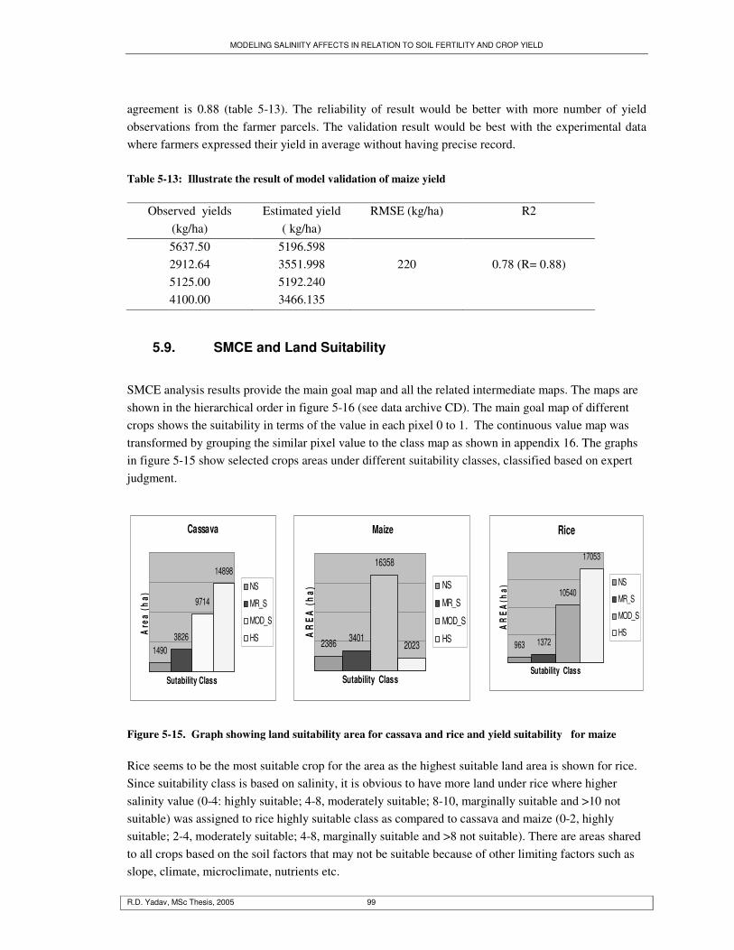
MODELING SALINIITY AFFECTS IN RELATION TO SOIL FERTILITY AND CROP YIELD
R.D. Yadav, MSc Thesis, 2005 99
agreement is 0.88 (table 5-13). The reliability of result would be better with more number of yield observations from the farmer parcels. The validation result would be best with the experimental data where farmers expressed their yield in average without having precise record. Table 5-13: Illustrate the result of model validation of maize yield
Observed yields (kg/ha)
Estimated yield ( kg/ha)
RMSE (kg/ha) R2
5637.50 5196.598 2912.64 3551.998 220 0.78 (R= 0.88) 5125.00 5192.240 4100.00 3466.135
5.9. SMCE and Land Suitability
SMCE analysis results provide the main goal map and all the related intermediate maps. The maps are shown in the hierarchical order in figure 5-16 (see data archive CD). The main goal map of different crops shows the suitability in terms of the value in each pixel 0 to 1. The continuous value map was transformed by grouping the similar pixel value to the class map as shown in appendix 16. The graphs in figure 5-15 show selected crops areas under different suitability classes, classified based on expert judgment.
Cassava
14903826
9714
14898
Sutability Class
Are
a (h
a)
NS
MR_S
MOD_S
HS
Maize
2386 3401
16358
2023
Sutability Class
AR
EA
(h
a)
NS
MR_S
MOD_S
HS
Rice
963 1372
10540
17053
Sutability Class
AR
EA
(ha)
NS
MR_S
MOD_S
HS
Figure 5-15. Graph showing land suitability area for cassava and rice and yield suitability for maize Rice seems to be the most suitable crop for the area as the highest suitable land area is shown for rice. Since suitability class is based on salinity, it is obvious to have more land under rice where higher salinity value (0-4: highly suitable; 4-8, moderately suitable; 8-10, marginally suitable and >10 not suitable) was assigned to rice highly suitable class as compared to cassava and maize (0-2, highly suitable; 2-4, moderately suitable; 4-8, marginally suitable and >8 not suitable). There are areas shared to all crops based on the soil factors that may not be suitable because of other limiting factors such as slope, climate, microclimate, nutrients etc.
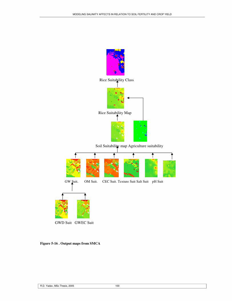
MODELING SALINIITY AFFECTS IN RELATION TO SOIL FERTILITY AND CROP YIELD
R.D. Yadav, MSc Thesis, 2005 100
Rice Suitability Class
Rice Suitability Map
Soil Suitability map Agriculture suitability
GW Suit. OM Suit. CEC Suit. Texture Suit Salt Suit pH Suit
GWD Suit GWEC Suit Figure 5-16 . Output maps from SMCA
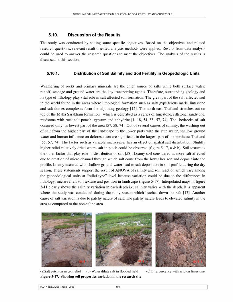
MODELING SALINIITY AFFECTS IN RELATION TO SOIL FERTILITY AND CROP YIELD
R.D. Yadav, MSc Thesis, 2005 101
5.10. Discussion of the Results
The study was conducted by setting some specific objectives. Based on the objectives and related research questions, relevant result oriented analysis methods were applied. Results from data analysis could be used to answer the research questions to meet the objectives. The analysis of the results is discussed in this section.
5.10.1. Distribution of Soil Salinity and Soil Fertility in Geopedologic Units
Weathering of rocks and primary minerals are the chief source of salts while both surface water: runoff, seepage and ground water are the key transporting agents. Therefore, surrounding geology and its type of lithology play vital role in salt affected soil formation. The great part of the salt affected soil in the world found in the areas where lithological formation such as salt/ gypsiferous marls, limestone and salt domes complexes form the adjoining geology [12]. The north east Thailand stretches out on top of the Maha Sarakham formation which is described as a series of limestone, siltstone, sandstone, mudstone with rock salt potash, gypsum and anhydrite [1, 18, 54, 55, 57, 74]. The bedrocks of salt occurred only in lowest part of the area [57, 58, 74]. Out of several causes of salinity, the washing out of salt from the higher part of the landscape to the lower parts with the rain water, shallow ground water and human influence on deforestation are significant in the largest part of the northeast Thailand [55, 57, 74]. The factor such as variable micro relief has an effect on spatial salt distribution. Slightly higher relief relatively dried where salt in patch could be observed (figure 5-17, a & b). Soil texture is the other factor that play role in distribution of salt [58]. Loamy soil considered as more salt-affected due to creation of micro channel through which salt come from the lower horizon and deposit into the profile. Loamy textured with shallow ground water lead to salt deposition in soil profile during the dry season. These statements support the result of ANOVA of salinity and soil reaction which vary among the geopedological units at “relief-type” level because variation could be due to the differences in lithology, micro-relief, soil texture and position in landscape (figure 5-17). Interpolated maps in figure 5-11 clearly shows the salinity variation in each depth i.e. salinity varies with the depth. It is apparent where the study was conducted during the rainy season which leached down the salt [17]. Another cause of salt variation is due to patchy nature of salt. The patchy nature leads to elevated salinity in the area as compared to the non-saline area.
(a)Salt patch on micro-relief (b) Water dilute salt in flooded field (c) Effervescence with acid on limestone Figure 5-17. Showing soil properties variation in the research site
MODELING SALINIITY AFFECTS IN RELATION TO SOIL FERTILITY AND CROP YIELD
R.D. Yadav, MSc Thesis, 2005 102
Similarly, scores of factors lead variation in pH since it depends on the parent material, precipitation, and management. Under the influence of saline ground water in presence of sodium and calcium, pH do not go higher than 8.5 due to several outcomes of an complex reaction [12]. High pH could also be possible when sodium solution is removed by leaching the clay-sodium where sodium has tendency to exchange with hydrogen from the water as hydrogen adsorbed leaving hydroxyl ion in salutation [12]. When aluminium and hydrogen takes the place of sodium then pH will become low and pH of the lower soil profile could be higher. All these cause variation in pH. This process could be found in the research area which is having diverse landforms. The similar study done by Pishakar (2003) on analysis of the relationship between soil salinity dynamics and geopedologic properties of the Goorband area in Iran has found the similar results of variation of soil salinity and pH in different geopedologic units [75]. However, the ANOVA results of OM and CEC are non-significant. This could be the cause of little observations in each landform unit.
5.10.2. Relationships of Soil Physico-chemical Properties
Occurrence of saline soil is common in arid and semi arid regions of the world. Out of several causes, mismanagement can be named as a result of which fertile soils become saline leading to soil productivity reduction and harm to the environment [1, 12, 74]. In the northeast of Thailand agricultural area suffers from salinity problem [1, 57, 74]. To manage saline soils, it is needed to understand the causes and mechanisms of salinization process. Organic matter application is one of the management practices applied in slightly and moderately saline soil [74]. Therefore, in order to see the relationship between EC and OM, the correlation and regression analysis were conducted. The result is statistically non-significant negative relationship. Therefore, there is no effect of organic matter over salinity except it adds or improves soil fertility and soil CEC [74, 76]. The similar result has established in a study of using cow dung in salt affected area of Thailand [54]. The relationship between CEC with both OM and clay are significant (table 5-4 and 5-5). Organic matter has humus which acts as an exchangeable site as it has negative charged on its outer surface as in clay. The relationship between CEC with organic matter and clay content resulted logistic and MMF model in surface and subsurface layer of soil. The relationship between these variables are logically follow the trend of natural phenomenon as the graph in figure 5-4 and 5-5 clearly shows the CEC increases with increase with OM and Clay almost linearly in the beginning that become asymptote after reaching to certain level. It is obvious in the nature. Increase of independent variables (CEC0 lead to increase of dependent variable (OM and clay) up to their maximum limit then it will remain constant. Therefore, these models could be used to predict CEC from the easily measurable soil properties (OM and clay). The significant multiple regression model of CEC against the OM and clay best be described the soil fertility. The root system of the plant varies from crops to crops but most active part of the root system is confined to surface layer of the soil. Therefore, surface layer fertility model could be applied in predicting soil fertility.
MODELING SALINIITY AFFECTS IN RELATION TO SOIL FERTILITY AND CROP YIELD
R.D. Yadav, MSc Thesis, 2005 103
5.10.3. Spatial Distribution of Salinity
The variogram model of electrical conductivity shows lower nugget effect in surface layer. Nugget effect increases with depth. It is the indication of moderate to weak spatial dependency with depth, showing that spatial dependency could be shorter than the sampling distance. The variogram of pH of each depth shows a weak spatial dependence and a high nugget, showing that spatial variability is nearly the same over the whole area. This is probably related to variability at scales smaller than the average sampling interval and can limit the results of the methodology applied. The validation result of the different interpolation technique revealed that the moving average gives best result with high R2 value (table 5-10) with the data sets. Kriging maps are smoother than the moving average and the RMSE of kriging is slightly lower. The areas nearer to the points noticeably show value closes to the point value in all kinds of interpolated maps. The error map (appendix 14) of the kriging of each depth is evidently shows lower error value which is the indication of top estimates in the space. The area far away shows higher error values. The salinity distribution of moving average corresponding the geopedological units compare to other maps. The similar results has revealed in the salinity study in Iran [69, 75]. Therefore, moving average could be the best interpolation method with little observation points. The interpolation technique were applied in this study without considering the landscape structure and none of the interpolation technique gave better result as R2 is not very high. The different part of the landscape of the area could be better described in terms of separate semi-variogrames rather than an average variogram for the whole area [77].
5.10.4. Spatial Modelling
The spatial distribution of electrical conductivity (EC) shows significant variation at all three soil depths in the study area. The surface layer shows highest variation. The salinity in both hot spot and salinity class shows similar pattern of salinity with depths (see Figure 5-10 and figure 5-11). However, hot spot was not noticed in the third layer (60-90 cm) of soil. Salinity class map (see figure 5-11) and salinity hot spot map (see Figure 5-10) visibly show the extent of salinity increases with depths. The salinity value could be lower but the extent is high. The salinity extent in lower landscape area as shown by the result is high. It is because the area receives runoff water from the recharge area and also has shallow ground water which lead to capillary rises during the dry period [1, 12, 19, 25, 54, 55, 58, 78, 79]. The salinity and hot spot map in this study shows the higher salinity value in low laying rice growing area. Similar study on salinity in Iran and Thailand [58, 69, 78, 79] revealed the result that low land having shallow ground water encompasses higher salinity. The study in Iran, have found higher salinity in surface layer where as this study shows higher salinity in subsoil. It is obvious where the study was conducted in rainy season where rain water leached down the salt to lower zone. The Iranian study was conducted during the dry period [69, 75]. Therefore, this result could be the tool for the indication of salinity area where chances of crop failure could be high. The extent of the alkaline, as given in table 5-12, is increased with the depth. The reason could be the same as explained under the variation of pH in saline soil [12]. The largest part of the area belongs to the slightly acidic class. This class decreases with depth and slightly alkaline to strongly alkaline class
MODELING SALINIITY AFFECTS IN RELATION TO SOIL FERTILITY AND CROP YIELD
R.D. Yadav, MSc Thesis, 2005 104
increases with the depth. One of the reasons of variation of pH under saline condition could be pH increases under submerged condition where study was done during the rainy season. Reduction under submerged condition lead to accumulation of carbon dioxide, ammonium, manganese and ferrous hydroxide [54].The hydroxides that occur reacts with hydrogen ion in the soil solution and with the soil colloid resulting rise of the pH [54].
5.10.5. Result of Climate Generation (ClimGen)
The ClimGen is the sub-model of the CropSyst which is used to generate the future climate for the prediction or forecasting of the climate. This could be used as inputs in the model for weather file and yield could be forecasted assuming other inputs are same. Since the daily required climatic data of the study area was not available, five years daily climatic data along with the geographical location was used to simulate the climate for ten years period (2003 to 2012). The simulated climatic data can be seen in data archive. The sub model of CropSyst generates the required climatic parameters. Some of the generated parameters was seems to be unreliable where it shows negative atmospheric temperature which does not exist in the country. The mean daily temperature data (2003) of the area is the evident to prove unreliability of generated data.
5.10.6. Simulated Result of the Model under Different Degree of Salinity
The model simulated the crop yield with the use of the input parameters prepared with the help of primary and secondary data. There are three main crops: cassava, rice and maize, have been growing in the study area. The model requires many experimental data. Since parameters for maize was available, the model was used to simulate the maize yield based on the soil fertility and salinity considering local management practices and generated climatic data. The Model simulates the crop yield as given in table 5-11. The simulated crop yield output is very low in comparison to the farmer yield which was collected during the field work. Researchers have used this model in field of study: crop yield biomass estimation, nitrogen uptake, impact of tillage and water balance successfully in different parts of the world [24, 28, 34, 42, 61, 80]. Considering these application, the input parameters were thoroughly checked to find the possible mistake that could have been done during data entry. There are some unreliable defects could be recognized in the generated data. The recognized defects are climate generation, parameters generated or estimated from soil texture, simulation from different folders. a. Impact of climate on simulated yield The biophysical model simulates the growth of the crops. This mainly depends on soil available moisture. It is the medium to absorb the nutrients and also transport the manufactured product in the leaf (see also chapter 2). The effect of salinity also related with the soil moisture. Increase in salinity has effect on osmotic potential and ultimately to the plant growth. The soil moisture could be maintained either by irrigation or depends on weather condition of the area. The weather plays main role in the study area, since there is no irrigation water available and crop cultivation totally depends on rain fall of the area. The ground water could be the source of irrigation which has limitation of high salt concentration [54, 58, 74]. Therefore, rainfall is the main source of soil water for the plant growth

MODELING SALINIITY AFFECTS IN RELATION TO SOIL FERTILITY AND CROP YIELD
R.D. Yadav, MSc Thesis, 2005 105
and crop yield. In a study by Katerji et al (2003) [36], concluded that there is no significant difference in yield response of corn under salinity and drought condition [36]. The result in table 5-12 on potential and actual evapotranspiration is the indication of the available water for the particular season to the plant. Higher potential evapotranspiration compared to actual evapotranspiration clearly indicates the soil water deficit. Soil water deficit leads to water stress to the plant. It has negative effect on growth and finally reduces the crop yield [27]. The simulated precipitation data may not be reliable due to limitation of available data. One of the shortcomings of the inputs of the climatic generated data was the non-availability of the required data for the climate generation. The model needs to have 25 years of real precipitation, 10 years of real temperature and five year’s complete solar radiation as an inputs for reliable data generation[33]. Since five years data were available, climate was generated on these bases. The generated data has a lot of variation in temperature, solar radiation and slight in wind speed. The simulated temperature of some days has dropped down to the negative value. Solar radiation, relative humidity and wind speed simulation are not uniform. There are many fluctuations on a number of days which is not consistent to the local condition (see data archive CD). Since it has option to generate daily data from the monthly data, the climate was generated with the use of this option. This also did not give better result. CropSyst modeller (personal communication) clarifies that five years climate data is not appropriate enough for ClimGen for climate generation. b. Soil texture and model simulation Soil texture is the basis of soil water calculation in the model. It has facility to calculate soil water parameters: available water, field capacity, permanent wilting point, bulk density and air entry potential. The model could indicate some of the texture simulated parameters as non reasonable value. The parameters: bulk density, air entry potential, moisture available at field capacity and clay percentage are those shown as not reasonable value by the model. Since the model shows unreliable value of the texture simulated parameters that could be the cause of having lower simulated yields where these are important factors of simulated crop production. The soil texture analysis report has taken from the laboratory and pH analysis was conducted with a reliable pH meter. Some of the texture percentage value for the calculation of soil moisture, air entry potential and pH higher than 8.5 shows invalid value by the model. These soil variables were analyzed with reliable laboratory which can possibly be found in the soils of the real world. Therefore, the model response to the texture as invalid could be the limitation of the model. Further, The CropSyst modeller in his mail explained that model shows unreliability but simulation would not be affected. c. Salinity and simulation yield The model was run with the geopedologic units on which maize was seen during the field trip. Some units have higher salinity. Then the model was also run with one of the higher value of salinity in top soil. The model showed invalid value for the ECe 25 dS/m but it was run and yield of the crop dropped down to 7.76 kg/ha (table 5-12). This means the model works and simulate under salinity condition. According to last email from the modeller, CropSyst could not perform well under groundwater
MODELING SALINIITY AFFECTS IN RELATION TO SOIL FERTILITY AND CROP YIELD
R.D. Yadav, MSc Thesis, 2005 106
salinity. It performs well under irrigated salinity cases. The sensitiveness of the model against the salinity has discussed under sensitivity analysis. d. Crop parameters and model simulation
The model is required many crop parameters as input to simulate the yield. The input crop parameters used are from the secondary source. They were collected from field work, some from the manual and rest from literature of study with this model in different part of the world [24, 28, 33]. Crop parameters have effect on the crop yield where some of these could be varied from location to location and among the cultivars [24, 28]. There are site specific parameters which could give better performance if experiment run in the area or possible to study in the local research area. Therefore, experimental data on crop could be the one option to improve the simulation. e. Modification of parameter and simulated result The climatic parameters were normalized in order to correct the climatic variation. The model was run which did not provide simulated yield. This might be the normalization effects differently to maximum and minimum climatic variables which might not fit with the model system. The simulated climatic data and date of different stages of growth of DSAT model used to observe the result of simulation. Climatic data was used as weather file and date of growth stages were used to calibrate the phenology heat requirement with the supplied crop calibrator of CropSyst. These parameters applied for the simulation of the crop yield. The replacing of this parameter resulted higher yield (2471.69 kg/ha) in comparison to previous result (770.60). The Priestley-Taylor evapotranspiration method was applied here whereas Penman-Monith evapotranspiration method was used in previous simulation.
5.10.7. PS123 and simulated yield
PS 123 is the crop growth simulation model of WOFOST family [38, 39]. The model is applied in various countries under different climatic situation in various crops. The yield result of the model is significantly correlated with the observed yield of the farmers (R2 = 0.78). Similar studies in China with same maize cultivar and also other cultivar has significantly simulated the maize yield [40]. Therefore, the performance of the model could be applied in similar studies. However, reliability of results could be expected with more yield observations from the farmer parcels where number of observations was used to validate the result was small. The model gave best result with 213 Julian planting date but model performance was poor with other planting date that was also used in the site. Therefore, the planting date best in the study site with this sets of climatic and crop data could be 213 Julian day. Further, model is well performed with different degree of salinity and maize yield is severely affected with salinity level beyond 8 dS/m in most soil units which is supported by several studies in different parts of the world [12]. The result shows clay loam texture soil gives higher and less affected with soil salinity. It could be the effect of higher CEC and water holding capacity of the soil that delays in stress.

MODELING SALINIITY AFFECTS IN RELATION TO SOIL FERTILITY AND CROP YIELD
R.D. Yadav, MSc Thesis, 2005 107
The model was tried to simulate the yield of cassava and rice with default crop parameters by changing total heat requirement and planting time. It simulates the cassava yield that is low but it did not performed well with rice. Since crop parameters vary from location to location that may lead to this result. Therefore, true site specific crop parameters could simulate reliable results.
5.10.8. Land suitability with SMCE as a GIS tool
In the real world situation, the issue of obtaining data for decision making in environmental and natural resources management is a complex one. Now a days, remote sensing and GIS technology have offered a great potential to captured the data from variety of earth observation platforms and incorporate them in a spatial manner [48-50]. It also facilitates appropriate technology for data extraction and storage, data management and manipulation, and visualization [48]. But they lack in analytical capabilities in order to support management and decision making process[48, 49]. GIS with its technology offer the opportunity for natural resources managers to easily combine and modify or manipulate data in order to meet the needs of making decisions about the environment and natural resources. As a result the SMCE functionality has been developed as easy and user friendly tool to predict suitable areas in dynamic environmental conditions. Scores of factors have to consider in development, evaluation, planning in decision making process for land evaluation and management processes [49]. The factor here considers for agricultural land suitability are soil properties such as soil organic matter content, soil EC, pH, groundwater depth and salinity, and CEC. Though these factors alone may not be sufficient to make decision on land suitability for different agricultural crops because their availability vary from place to place yet the results here could be used to indicate the probable land suitable for agriculture based on soil salinity point of view. The suitability maps clearly show that highly saline areas are not suitable for agriculture purposes especially for the selected crops. Reliable results could be expected from combining many factors that could be time consuming, costly and may not be available. Other than this, the value or weigh assigned in this process is based on expert judgment. Therefore, results could vary from person to person. These seem to be the drawbacks of this method. However, SMCE with analytical functionality of GIS environment support the decision makers to solve the spatial decision problems [49]. This functionality in ILWIS environment has been applied in the environment field considering many factors in a user friendly way [49].
5.10.9. Salinity Sensitiveness of the CropSyst Model
The sensitivity result of the CropSyst model against salinity is best be described with third order polynomial fitted model with R2 = 0.9466. The yield is drastically decreased with each unit increase of EC value from 3 to 9. The decreased in yield is almost 50 percent with each unit increment of EC
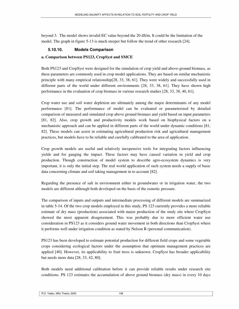
MODELING SALINIITY AFFECTS IN RELATION TO SOIL FERTILITY AND CROP YIELD
R.D. Yadav, MSc Thesis, 2005 108
beyond 3. The model shows invalid EC value beyond the 20 dS/m. It could be the limitation of the model. The graph in figure 5-13 is much steeper but follow the trend of other research [24].
5.10.10. Models Comparison
a. Comparison between PS123, CropSyst and SMCE Both PS123 and CropSyst were designed for the simulation of crop yield and above-ground biomass, as these parameters are commonly used in crop model applications. They are based on similar mechanistic principle with many empirical relationship[28, 33, 38, 61]. They were widely and successfully used in different parts of the world under different environments [28, 33, 38, 61]. They have shown high performance in the evaluation of crop biomass in various research studies [28, 33, 38, 40, 61]. Crop water use and soil water depletion are ultimately among the major determinants of any model performance [81]. The performance of model can be evaluated or parameterized by detailed comparison of measured and simulated crop above ground biomass and yield based on input parameters [81, 82]. Also, crop growth and productivity models work based on biophysical factors on a mechanistic approach and can be applied in different parts of the world under dynamic conditions [81, 82]. These models can assist in estimating agricultural production risk and agricultural management practices, but models have to be reliable and carefully calibrated to the area of application. Crop growth models are useful and relatively inexpensive tools for integrating factors influencing yields and for gauging the impact. These factors may have caused variation in yield and crop production. Though construction of model system to describe agro-ecosystem dynamics is very important, it is only the initial step. The real world application of such system needs a supply of basic data concerning climate and soil taking management in to account [82]. Regarding the presence of salt in environment either in groundwater or in irrigation water, the two models are different although both developed on the basis of the osmotic pressure. The comparison of inputs and outputs and intermediate processing of different models are summarized in table 5-14. Of the two crop models employed in this study, PS 123 currently provides a more reliable estimate of dry mass (production) associated with maize production of the study site where CropSyst showed the most apparent disagreement. This was probably due to more efficient water use consideration in PS123 as it considers ground water movement in both directions than CropSyst where it performs well under irrigation condition as stated by Nelson R (personal communication). PS123 has been developed to estimate potential production for different field crops and some vegetable crops considering ecological factors under the assumption that optimum management practices are applied [40]. However, its applicability to fruit trees is unknown. CropSyst has broader applicability but needs more data [28, 33, 42, 80]. Both models need additional calibration before it can provide reliable results under research site conditions. PS 123 estimates the accumulation of above ground biomass (dry mass) in every 10 days
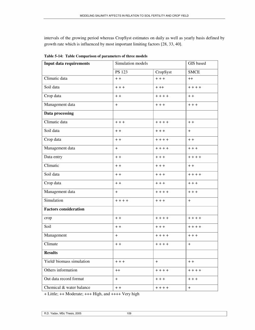
MODELING SALINIITY AFFECTS IN RELATION TO SOIL FERTILITY AND CROP YIELD
R.D. Yadav, MSc Thesis, 2005 109
intervals of the growing period whereas CropSyst estimates on daily as well as yearly basis defined by growth rate which is influenced by most important limiting factors [28, 33, 40]. Table 5-14: Table Comparison of parameters of three models
+ Little; ++ Moderate; +++ High, and ++++ Very high
Simulation models GIS based Input data requirements
PS 123 CropSyst SMCE Climatic data + + + + + ++
Soil data + + + + ++ + + + +
Crop data + + + + + + + +
Management data + + + + + + +
Data processing
Climatic data + + + + + + + + +
Soil data + + + + + +
Crop data + + + + + + + +
Management data + + + + + + + +
Data entry + + + + + + + + +
Climatic + + + + + + +
Soil data + + + + + + + + +
Crop data + + + + + + + +
Management data + + + + + + + +
Simulation + + + + + + + +
Factors consideration
crop + + + + + + + + + +
Soil + + + + + + + + +
Management + + + + + + + +
Climate + + + + + + +
Results
Yield/ biomass simulation + + + + + +
Others information ++ + + + + + + + +
Out data record format + + + + + + +
Chemical & water balance + + + + + + +

MODELING SALINIITY AFFECTS IN RELATION TO SOIL FERTILITY AND CROP YIELD
R.D. Yadav, MSc Thesis, 2005 110
The PS 123 considers total heat requirements for phenological development, constant soil types in all depths where CropSyst have sub models considering phenological development of different crop growth stages, soil nitrogen, and soil moisture of different layers, CEC and organic matter content. Crop growth during each phenological stage is regulated by the estimated adequacy of the temperature, moisture, radiation and nitrogen regimes. Planting date and soil moisture reserves at planting are required to initiate CropSyst. In summary, PS 123 performs well with changing parameters: total heat requirement, planting time and seed rate as compared to CropSyst. The reason for underestimates of crop yield could be the climatic data and crop data. These data were from the secondary source. The metrological data was from the area far from the research site that may not perform well at the local condition. Therefore, result could be better with experimental data of the whole season and also climatic data with local meteorological station. For GIS oriented modelling SMCE of ILWIS can be used [49, 50]. This is not meant for simulating that is, SMCE application assists and guides a user in doing SMCE in a spatial way. Also, SMCE with analytical functionality of GIS environment support the decision makers to solve the spatial decision problems [49]. The input for the application is a number of maps of a certain area (so-called 'criteria' or 'effects'), and a criteria tree that contains the way criteria are grouped, standardized and weighed. The normalization is done by expert judgment that may lead to variation of results from expert to expert. It needs a lot of data to have appropriate suitability map. The results obtained from the SMCE may be site specific and may not be directly applicable to other areas. It requires many layers that may need more information which may necessitate more budgets. Creating and combining of all the input layers may reduce the efficiency of computer.
b. Comparison of models outputs (Mechanistic model and GIS model) All the different models applied to assess the yield of maize showed similar pattern (figure5-18). It is interesting to note that in areas where the mathematical and crop yield model showed low yield, SMCE also indicated that those areas have low suitability for maize production. Crop simulation model and mathematical model estimates the yield potential of areas whilst SMCE demarcates suitable area for crop production. After the analysis of all the different models applied to assess the maize yield showed similar pattern. The yield area resulted from different models were different. However, the results obtained from PS 123 and mathematical model was similar whereas it was different with the SMCE. The differences in area could be due to the criteria assigned to different models were different. The SMCE map was generated on the basis of weigh assigned to different criteria on expert judgment. More weigh was assigned to soil salinity and also the criteria value was assigned in the range (see also section 4.11). The other two models (PS 123 and Mathematical) classes were generated based on the point values. PS123 considers the soil texture class whereas mathematical model was based on point
MODELING SALINIITY AFFECTS IN RELATION TO SOIL FERTILITY AND CROP YIELD
R.D. Yadav, MSc Thesis, 2005 111
soil fertility parameters. Therefore, each of these models could be applied based on the available data and aim of the users. Since data for validation was not appropriate enough, best model could be evaluated with more number of observations.
(a)
©
(e)
(b)
(d)
(f) Figure 5-18. Maize yield from SMCE (a, b), Multiple regression (c, d) and PS 123(e, f)
Limitations and Assumptions
� All soil properties data were assumed to be normally distributed. � The default crop parameters and soil parameters available with the models were assumed to be
similar and were used in this study. � Relevant climate parameters for the climate generation were only available for 5 years which
was insufficient for the climate generator to generate climatic data for the mechanistic model applied to this study.
� Crop yield data of the parcel was limitation in this study. � Soil salinity (EC) and soil fertility parameters such as CEC, OM, and pH and soil texture were
considered in crop yield assessment in this study. However, management practices and other nutrients effects could not be underestimated in crop yield assessment.
MODELING SALINIITY AFFECTS IN RELATION TO SOIL FERTILITY AND CROP YIELD
R.D. Yadav, MSc Thesis, 2005 112
6. Conclusions and Recommendations
The research concludes with following remarks looking at the research questions based on the objectives. Q1. How do soil salinity and soil fertility parameters such as OM, CEC, and pH vary in the geopedological units? To answer this question, stratified (based on geopedologic unit) random sampling was done to cover all geopedologic units. The soil properties were compared using side by side boxplots at “relief- type” level. Stratification significance was tested with ANOVA. The result of stratification significance test (table 5-1) showed that soil properties such as log EC and pH significantly vary between geopedologic units in all three soil depths, whereas, CEC and OM varied insignificantly. Therefore, it was concluded that the geopedological approach could be an appropriate one, which also minimizes the cost for collecting samples for soil maps and undertaken necessary analyses. Recommendation In this study, only few observations covered the existing geopedologic units resulting in their improper representation. Thus increase in number of observations covering the existing geopedological units could significantly enhance the analysis result. Q2. How does soil salinity affect crop productivity? It is well known that salinity has adverse effect on crop yield through affecting the osmotic potential balance between soil and plant. The relationship was expected to be established based on simulation result of crop growth model. The model is structured in such a way that it simulates the crop yield under different degrees of salinity, with weather, crop biophysical, soil and management as input data. The required data for the research were collected based on stratification (see section 4.2). Input data applied to the simulation model resulted crop yield under different degrees of salinity. The simulation result showed that the crop yield decreases with increasing salinity (see section 5.5, appendix 7 and 16). CropSyst did not perform well whereas PS 123 (DOS version) performed well. In the later stage of the study I came to understand that PS 123 has been recently converted and exist in windows. The correlation of the crop yield simulated by the PS 123 model have significant R2 of 0.8 with the yield
MODELING SALINIITY AFFECTS IN RELATION TO SOIL FERTILITY AND CROP YIELD
R.D. Yadav, MSc Thesis, 2005 113
data collected from the farmers (RMSE 200 kg/ha). This helps to conclude that the PS 123 could be applied in similar studies. Recommendation Since, numerous yields related variables (crop growth, phenology, crop morphology, harvest, nitrogen band residue) as well as soil variables are taken into account by CropSyst, the performance would be expected to be better with experimental data. However, PS 123 could also be used in similar studies assuming constant management practices (figure 2-11). The validation was done with few observations that may not be so convincing. Better results would be expected with farmers parcel based yield observations. Q3. What is the relationship between crop productivity and soil fertility variables? It is a well known fact that high crop productivity is related to higher soil fertility, provided other factors are optimum. Mechanistic simulation models are capable to consider soil fertility parameters in crop growth simulations. The models used in the study have facility to simulate crop growth and production, taking soil fertility into account. PS 123 does not directly consider the soil fertility parameters in simulation but it considers the soil types which has significant relationship with soil properties that determine soil fertility (CEC). The model simulates higher yield with heavy soil despite higher salinity (appendix 7 and 16). The laboratory analysis results show that heavy soils (high clay content) have significant positive relationship with CEC (see also section 5.16). The results showed positive relationship between crop yield and soil fertility that may translate in higher crop yield. Further, significant result (p<0.05, R2 = 0.795) of mathematical model (regression model) developed by establishing relationship between maize yield and soil properties (see section 5.7.2) revealed that crop yield is increased with increasing soil fertility. CropSyst model was intended to use to answer this question by establishing the relationship between crop yield and soil properties. The model is meant to simulate crop yield considering soil fertility while taking management practices into account. Since CropSyst simulation results did not correspond with the farmers yield, personal communication was made with the modeller (Nelson R.). The model showed some errors which were agreed by the modeller (personal communication). Also the sources of the secondary data used in crop simulation were not from the study area. Recommendation CropSyst considers most of the yield predictors such as climate, crop biophysical, soil and managements. Therefore, better and reliable results could be expected with experimental data.
MODELING SALINIITY AFFECTS IN RELATION TO SOIL FERTILITY AND CROP YIELD
R.D. Yadav, MSc Thesis, 2005 114
Q 4. What is the relationship between soil salinity and soil organic matter content? Farmers are asked to apply organic manures in order to manage saline soils. Keeping this in mind, the research question was proposed to establish and test the relationship between soil salinity and soil fertility (especially with organic matter content). The correlation analysis was performed to observe the relationship between organic matter content and soil salinity (EC). Non-significant correlation analysis results between EC and OM revealed that soil organic matter does not have significant role on EC (section 5.1.3, table 5-3). Therefore, the non-significance result helps to conclude that organic matter could be the sources of plant nutrients and its positive impacts on soil properties support plant growth environment. Therefore, organic manure could not be used as direct soil amendment but it can be used as indirect benefit to the plant growth and development. However, significant correlation results (section 5.1.6) between CEC and soil properties (OM and Clay content) could be applicable to estimate CEC (time consuming variables and high cost involved) with the combination of easily measurable and low cost involved soil properties such as OM and clay (pedotransfer function). Recommendation Practical constraints such as available time and economic constraints limited the observations for organic matter. The collected data are insufficient to represent the whole study area which is undulating and having numerous landform units. The relationship could be expected to be better with more representative observations. This could be the subject for further research. The collected data could be used for future study as OM of the soil is not exposed to change. Q5. How does soil salinity and soil fertility variables correlate spatially? Scores of factors are responsible for soil salinity and soil fertility. EC is considered as soil salinity variable and soil pH is considered as soil fertility variable. Since the number of observations of these variables thought to be reasonably high (a total of 71 observations), OK and KED techniques were used to observe their spatial relationship on the surface. The erratic nature of these variables could not result a good variogram (section 5.3.1, appendix 12). Spatial dependency of these variables would be expected on shorter distances than the current sampling interval. However, when observation number is low, as in the above case, out of several interpolation techniques, moving average (inverse distance) method gives significant results for both variables in all soil depths (table 5-10). Both soil salinity and soil pH increases with soil depths (figure 5-3). Some part of the site shows higher values for both variables where part of the site has higher pH and low salinity. The interpolated map and classified maps (figure 5-7, 5-11 and 5-12) show spatial pattern of soil salinity and pH. Therefore, it can be concluded that moving average would be the best interpolation method explaining the spatial pattern of soil properties with low number of observations (a rough limit of 150 observations has been mentioned). This result could be applied in landuse planning for sustainable agriculture.

MODELING SALINIITY AFFECTS IN RELATION TO SOIL FERTILITY AND CROP YIELD
R.D. Yadav, MSc Thesis, 2005 115
Recommendation Moving average method gives the best result whereas OK and KED geostatistical show moderate spatial dependency with large unexplained (nugget) variance. This shows that their spatial dependency could be of shorter distances than the current sampling intervals i.e. the number of observations is insufficient. Therefore, more observation along with nested sampling may possibly give better results. Q6. How accurately can soil salinity and soil fertility be evaluated? Considering the aim of the research, salinity hotspot map is presented using geostatistical technique and GIS. Soil salinity and soil reaction class maps are the result of slicing operation of moving average interpolation map. The hot spot areas indicated in the map (figure 5-10) represent salinity level beyond the threshold value and area below salinity threshold. Similarly, soil salinity and soil reaction maps (figure 5-11 and 5-12) give insight about the area having different level of pH and salinity. On the basis of this information different landuses strategies could be identified to sustain the agricultural production of the area. Recommendation Maps used on evaluation of the soil salinity and soil reaction (as one of the soil fertility indicators) are the results of the interpolated map. It was observed and realized that the best interpolation map with soil properties having spatial dependency resulted with more observations and nested sampling. Therefore, the evaluation result also could be expected better with more observations and different interpolated techniques. Q7. How accurately can crop yield be assessed by CropSyst model and what is its difference with PS123 and GIS oriented model? Both CroSyst and PS 123 are mechanistic based crop growth models. They work on similar principle depending on extensive climate, soil and crop data. The two models were applied to simulate maize yield under different degree of salinity. The CropSyst simulates much lower yield than that of the observed yield. The PS 123 gave significant result with observed yield (R2=0.78) i.e PS 123 simulates yields which is identical or higher than the observed yield. Therefore, PS123 could be applied to estimate maize yield in similar studies. PS 123 provides best result as compared to CropSyst but both models have their shortcomings (see section 5.10.10 and also table 5-14). CropSyst considers many yield variables including management inputs as compared to PS 123. Yield differences were observed among the GIS oriented models such as SMCE and mathematical models when both were used to predict maize yield under different degrees of salinity.

MODELING SALINIITY AFFECTS IN RELATION TO SOIL FERTILITY AND CROP YIELD
R.D. Yadav, MSc Thesis, 2005 116
SMCE is used to indicate areas likely to be suitable to a particular land use type. Within the study, SMCE prediction of suitable areas for maize production included urban areas and water bodies as unsuitable whereas PS 123 models include water bodies and urban areas in its prediction. The mathematical model combines actual point data and its highly significant result (R2=0.795) may be concluded that yield can be accurately assessed by integrating the outputs of mechanistic model with GIS, using real world data. SMCE is the result of many input layers of factors. Since factors weigh is determined by expert that plays significant role in outputs, it could be applied to a particular site based on available data and expert aims. Recommendation All models showed similar pattern of yield variation in relation to different degree of salinity as well as significant result with available parcel yield information. Since relevant parcel yield data are insufficient, models could not be validated with low number of observations. This is because of time constraints. Therefore, the model could probably be applicable in similar studies with sufficient observations.
Recommendations for the future research
� Temporal remote sensing data in combination with parcel yield and parcel based map could enhance salinization modelling.
� CropSyst model could give better simulation results with an experimental inputs data that can be used in assessing crop yield under different degrees of salinity.
MODELING SALINIITY AFFECTS IN RELATION TO SOIL FERTILITY AND CROP YIELD
R.D. Yadav, MSc Thesis, 2005 117
7. References:
1. Ghassemi F, Jakeman A.J., and Nix H.A., Salinization of land and Water Resources. 1995: University of New South Wales Press Ltd. Sydney, Australia and CAB International, Wallingford Oxon, UK.
2. USDA Natural Resources Conservation Service, Soil Quality Resource Concerns: Salinization. 1998, U. S. Department of Agriculture (USDA): Washington, DC.
3. Fitzpatrick, R., Rengasamy, P.,Merry, R.,Cox, J.,, Is dry land salinization reversible? 2001, University of Adelaide: Glen Osmond.
4. Metternicht, G.I., Zinck, J. A.,, Remote sensing of soil salinity: potentials and constraints. Remote Sensing of Environment, 2003. 85(1): p. 1-20.
5. Eswaran H., Lal R., and Reich P.F. Land degradation: An overview. 2001. Khon Kaen, Thailand: Oxford Press, New Delhi, India.
6. Grattan S. R. , Irrigation Water Salinity and Crop Production, A.A.E.f.N. Resources., Editor. 2002, University of California,Agriculture and Natural Resources Communication Services,Partnership with NRCS, ANR publication 8066: California.
7. Farshad A., A syllabus on desertification(Land degradation and conservation). 2003. 8. FAO, Extent and Causes of Salt-affected Soils in Participating Countries. 2000, FAO. 9. Fresco Louise O., Fertilizer and the future, in Spotlight. 2003. 10. Wiegand, C., Anderson, G., Lingle, S., Escobar, D.,, Soil salinity effects on crop growth and
yield - illustration of an analysis and mapping methodology for sugarcane. Special issue: vegetation stress II, 1996. Munich, Germany, 19-21 June 1995. Journal-of-Plant-Physiology. 1996, 148(3-4): p. 418-424.
11. Brady N.C. and Weil R.R., The nature and properties of soil. 1996, New Jersey: Prentice-hall international, inc.
12. Farshad A., Soil degradation;salinization/alkalinization;Lecture notes. 2000: ITC, Enschede. 13. Prasad R. and Power J.F., Soil Fertility Management for Sustainable Agriculture. 1997,
Florida: Lewish publisher,Boca Raton,Newyork. 356. 14. van Hoorn, J.W., Katerji, N., Hamdy, A., Mastrorilli, M.,, Effect of salinity on yield and
nitrogen uptake of four grain legumes and on biological nitrogen contribution from the soil. Agricultural Water Management, 2001. 51(2): p. 87-98.
15. Pathak H. and Rao D. L. N., Carbon and nitrogen mineralization from added organic matter in saline and alkali soils. Soil Biology and Biochemistry, 1998. 30(6): p. 695-702.
16. Assumption University, Agricultural Resources. 1995, Amarin Printing and Publishing Public Company Limited: Bangkok.
17. Soliman A., Detecting salinity in early stages using electromagnetic survey and multivariate geostatistical technique; a Case study of Nong Suang district, Nakhon Ratchasima, Thailand., in Geo-information Science and Earth Observation, Soil Information Systems for Sustainable Land Management. 2004, ITC: Enschede. p. 100.
18. LDD, Excursion program for the international symposium on paddy soil. 1996: Khon Kaen. 19. IRD and LDD project, Improving the management of salt-affected soils: the case of salaine
patches in rainfed paddy fields in Northeast Thailand http://www.mpl.ird.fr/ariane/Thailande/Home_page/IRD_Home_pagebottom.htm.
20. Dorota Z. H. and Forrest T. L., Soil Plant Water Relationships;University of Florida. 2003. 21. Taylor S., Dryland Salinity - Introductory Extension Notes. Second ed. 1993.
MODELING SALINIITY AFFECTS IN RELATION TO SOIL FERTILITY AND CROP YIELD
R.D. Yadav, MSc Thesis, 2005 118
22. Estes M., A Review of Salinity Stress on Plants; http://www.bio.davidson.edu/people/kabernd/seminar/2002/stress/Salinity%20Paper.htm. 2002.
23. Maas E.V. and Hoffman G.J., Crop salt tolerance current assessment. Irrigation Journal, Drainage Div. ASCE 103, 1977: p. 115-134.
24. FAO. A model for assessing crop response and water management in saline conditions. in Irrigation Scheduling: From Theory to Practice - Proceedings. 1995. Wash Rome, Italy,: FAO.
25. Parida, A.K., Das, A. B., Salt tolerance and salinity effects on plants: a review. Ecotoxicology and Environmental Safety, 2005. 60(3): p. 324-349.
26. Neumann, Salinity resistance and plant growth revisited. 1997: p. 1193-1198. 27. Lamsal K., Guna N.P., and Saeed M., Model for assessing impact of salinity on soil water
availability and crop yield. Agricultural Water Management, 1999. 41(1): p. 57-70. 28. Stockle, C.O., Donatelli M., and Nelson R., CropSyst, a cropping systems simulation model.
European Journal of Agronomy, 2003. 18(3-4): p. 289-307. 29. Yang, H.S., Dobermann, A., Lindquist, J. L., Walters, D. T., Arkebauer, T. J., Cassman, K. G.,,
Hybrid-maize--a maize simulation model that combines two crop modeling approaches. Field Crops Research, 2004. 87(2-3): p. 131-154.
30. Williams, J.R., Jones , C. A., Kiniry, J.R., Spanel, D.A,, The EPIC crop growth model. ASAE, 1989. 32(2).
31. Van Diepen, C.A., Van Diepen, C.A., W0lf, J., Van Keulen, H., Berkhout, J.A.A,, Land Evaluation: from intuition to quantification. Advances in soilsciences, 1991. 15: p. p. 139-204.
32. FAO, A computer programme for irrigation planning and management. 1992. 33. Stöckle C. O. and Nelson R., Cropping Systems Simulation Model, User's Manual. 2000,
Washington State University: Washington. p. 235. 34. Stockle, C.O., Campbell, G. S.,, Simulation of crop response to water and nitrogen: An
example using spring wheat. Transactions of the ASAE. 32(1): p. 66-74. 35. FAO, L.a.W.D., Water Resources, Development and Management Service. 2002, FAO. 36. Katerji, N., van Hoorn, J. W., Hamdy, A., Mastrorilli, M.,, Salinity effect on crop development
and yield, analysis of salt tolerance according to several classification methods. Agricultural Water Management, 2003. 62(1): p. 37-66.
37. Meinke H., et al., Increasing profits and reducing risks in crop production using participatory systems simulation approaches. Agricultural Systems, 2001. 70(2-3): p. 493-513.
38. Rossiter, D.G., Biophysical Models in Land Evaluation. 2003, International Institute for Geo-Information Science and Earth Observation (ITC), Enschede,
the Netherlands: Enschede. 39. Farshad, A., Analysis of integrated soil and water management practices within different
agricultural systems under semi - arid conditions of Iran and evaluation of their sustainability, in Earth Sciences. 1997, Publication No.57,: Enschede. p. 395.
40. Driessen P.M. and Konijn N.T., Land-use systems analysis. 1992, Wageningen: Wageningen Agricultural University. 230.
41. Nelson R., Climatic data generator user's manual. 2002, Biological System Engineering Department, Washington State University,.
42. Bellocchi G.1, S.N., Mazzoncini M. 2, Menin S 3., Using the CropSyst Model in Continuous Rainfed Maize (Zea mais L.) under Alternative Management Options. 2002.
43. Badini, O., Stockle, C. O.,Franz, E. H.,, Application of crop simulation modeling and GIS to agroclimatic assessment in Burkina Faso. Agriculture, Ecosystems & Environment, 1997. 64(3): p. 233-244.
44. Lang C., Kriging interpolation, Dept. of computer science,Cornell University. 45. Triantafilis J., Odeh I.O.A., and McBratney A.B., Five Geostatistical Models to Predict Soil
Salinity from Electromagnetic Induction Data Across Irrigated Cotton. Soil Sci Soc Am J, 2001. 65(3): p. 869-878.
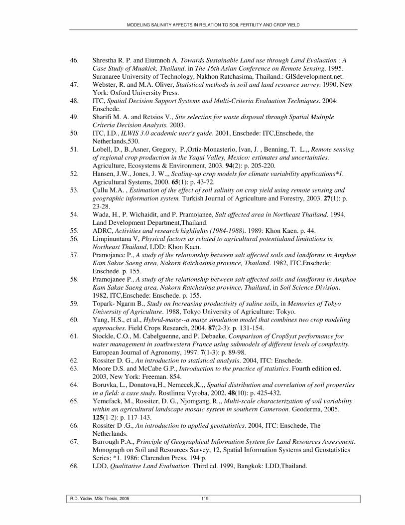
MODELING SALINIITY AFFECTS IN RELATION TO SOIL FERTILITY AND CROP YIELD
R.D. Yadav, MSc Thesis, 2005 119
46. Shrestha R. P. and Eiumnoh A. Towards Sustainable Land use through Land Evaluation : A Case Study of Muaklek, Thailand. in The 16th Asian Conference on Remote Sensing. 1995. Suranaree University of Technology, Nakhon Ratchasima, Thailand.: GISdevelopment.net.
47. Webster, R. and M.A. Oliver, Statistical methods in soil and land resource survey. 1990, New York: Oxford University Press.
48. ITC, Spatial Decision Support Systems and Multi-Criteria Evaluation Techniques. 2004: Enschede.
49. Sharifi M. A. and Retsios V., Site selection for waste disposal through Spatial Multiple Criteria Decision Analysis. 2003.
50. ITC, I.D., ILWIS 3.0 academic user's guide. 2001, Enschede: ITC,Enschede, the Netherlands,530.
51. Lobell, D., B.,Asner, Gregory, P.,Ortiz-Monasterio, Ivan, J. , Benning, T. L.,, Remote sensing of regional crop production in the Yaqui Valley, Mexico: estimates and uncertainties. Agriculture, Ecosystems & Environment, 2003. 94(2): p. 205-220.
52. Hansen, J.W., Jones, J. W.,, Scaling-up crop models for climate variability applications*1. Agricultural Systems, 2000. 65(1): p. 43-72.
53. Çullu M.A. , Estimation of the effect of soil salinity on crop yield using remote sensing and geographic information system. Turkish Journal of Agriculture and Forestry, 2003. 27(1): p. 23-28.
54. Wada, H., P. Wichaidit, and P. Pramojanee, Salt affected area in Northeast Thailand. 1994, Land Development Department,Thailand.
55. ADRC, Activities and research highlights (1984-1988). 1989: Khon Kaen. p. 44. 56. Limpinuntana V, Physical factors as related to agricultural potentialand limitations in
Northeast Thailand, LDD: Khon Kaen. 57. Pramojanee P., A study of the relationship between salt affected soils and landforms in Amphoe
Kam Sakae Saeng area, Nakorn Ratchasima province, Thailand. 1982, ITC,Enschede: Enschede. p. 155.
58. Pramojanee P., A study of the relationship between salt affected soils and landforms in Amphoe Kam Sakae Saeng area, Nakorn Ratchasima province, Thailand, in Soil Science Division. 1982, ITC,Enschede: Enschede. p. 155.
59. Topark- Ngarm B., Study on Increasing productivity of saline soils, in Memories of Tokyo University of Agriculture. 1988, Tokyo University of Agriculture: Tokyo.
60. Yang, H.S., et al., Hybrid-maize--a maize simulation model that combines two crop modeling approaches. Field Crops Research, 2004. 87(2-3): p. 131-154.
61. Stockle, C.O., M. Cabelguenne, and P. Debaeke, Comparison of CropSyst performance for water management in southwestern France using submodels of different levels of complexity. European Journal of Agronomy, 1997. 7(1-3): p. 89-98.
62. Rossiter D. G., An introduction to statistical analysis. 2004, ITC: Enschede. 63. Moore D.S. and McCabe G.P., Introduction to the practice of statistics. Fourth edition ed.
2003, New York: Freeman. 854. 64. Boruvka, L., Donatova,H., Nemecek,K.,, Spatial distribution and correlation of soil properties
in a field: a case study. Rostlinna Vyroba, 2002. 48(10): p. 425-432. 65. Yemefack, M., Rossiter, D. G., Njomgang, R.,, Multi-scale characterization of soil variability
within an agricultural landscape mosaic system in southern Cameroon. Geoderma, 2005. 125(1-2): p. 117-143.
66. Rossiter D .G., An introduction to applied geostatistics. 2004, ITC: Enschede, The Netherlands.
67. Burrough P.A., Principle of Geographical Information System for Land Resources Assessment. Monograph on Soil and Resources Survey; 12, Spatial Information Systems and Geostatistics Series; *1. 1986: Clarendon Press. 194 p.
68. LDD, Qualitative Land Evaluation. Third ed. 1999, Bangkok: LDD,Thailand.

MODELING SALINIITY AFFECTS IN RELATION TO SOIL FERTILITY AND CROP YIELD
R.D. Yadav, MSc Thesis, 2005 120
69. Naseri M.Y, Characterization of salt-affected soils for modeling sustainable land management in semi-arid environment: a case study in the Gorgan region, northeast Iran, in Faculty of sciences. 1998, University of Ghent: Ghent, Belgium. p. 321.
70. Neild R. E. and Newman J. E., Growing Season Characteristics and Requirements in the Corn Belt, Purdue University,Cooperative Extension Service, West Lafayette,
IN 47907. 71. Field crop research institute, A guide book for field crops production in Thailand. Second ed.
2001, Bangkok: Department of Agriculture, Ministry of agriculture and cooperatives, Bangkok, Thailand.
72. Tamaluddin S. and Kamaruzaman J., Remote Sensing (RS) and Geographic Information System (GIS) Technology for Field Implementation in Malaysian Agriculture*. 1999, Precision Agriculture Programme , Institute Bioscience,Universiti Putra Malaysia
43400 UPM Serdang, Selangor, Malaysia.: Selangor, Malaysia. 73. Eldeiry A. and Garcia L., Spatial Modeling using Remotesensing,GIS, and field data to Assess
Crop Yield and Soil Salinity. 2004, Colorado State University: Colorado. 74. Yuvaniyama A., Arunin S., and Takai Y., Management of saline soil in the northeast of
Thailand. Thai journal Agric. Sci. 29, 1996: p. 1-10. 75. Pishkar A., Analysis of relationship between soil salinity dynamics and geopedologic
properties; a case study of Goorband area,Iran., in Geo-information Science and Earth Observation, WRS, department. 2003, ITC: Enschede. p. 145.
76. Irshad M., Y.S., Enejia E., and Honna T., Influence of composted manure and salinity on growth and nutrient content of maize tissue. 2002, Tottori University: Tottori City.
77. Burrough P.A., Principle of Geographical Information System for Land Resources Assessment. 1986: Oxford University Press, New York. 193.
78. Soliman A.S., et al., Predicting salinization in its early stage, using electro magnetic data and geostatistical techniques : a case study of Nong Suang district, Nakhon Ratchasima, Thailand. 2004.
79. Farshad A. and Barrera-Bassols N., Historical anthropogenic land degradation related to agricultural systems : case studies from Iran and Mexico. 2003. 85(3-4): p. 277-286.
80. Donatelli, M., et al., Evaluation of CropSyst for cropping systems at two locations of northern and southern Italy. European Journal of Agronomy, 1997. 6(1-2): p. 35-45.
81. Eitzinger, J.a., Trnka ,M. b, Hosch, J. c,Zalud Z.b , Dubrovsky, M.d,, Comparison of CERES, WOFOST and SWAP models in simulating soil water content during growing seasonunder different soil conditions. Ecological modelling, 2004. 171: p. 223-246.
82. Kimble, J.M. Proceedings of the eighth International soil management workshop: Utilization of soil survey information for sustainable land uset. in Eighth International Soil Management Workshop. 1993. Oregon,California, and Nevada: Soil Conservation Service, National Soil Survey Center, USDA.
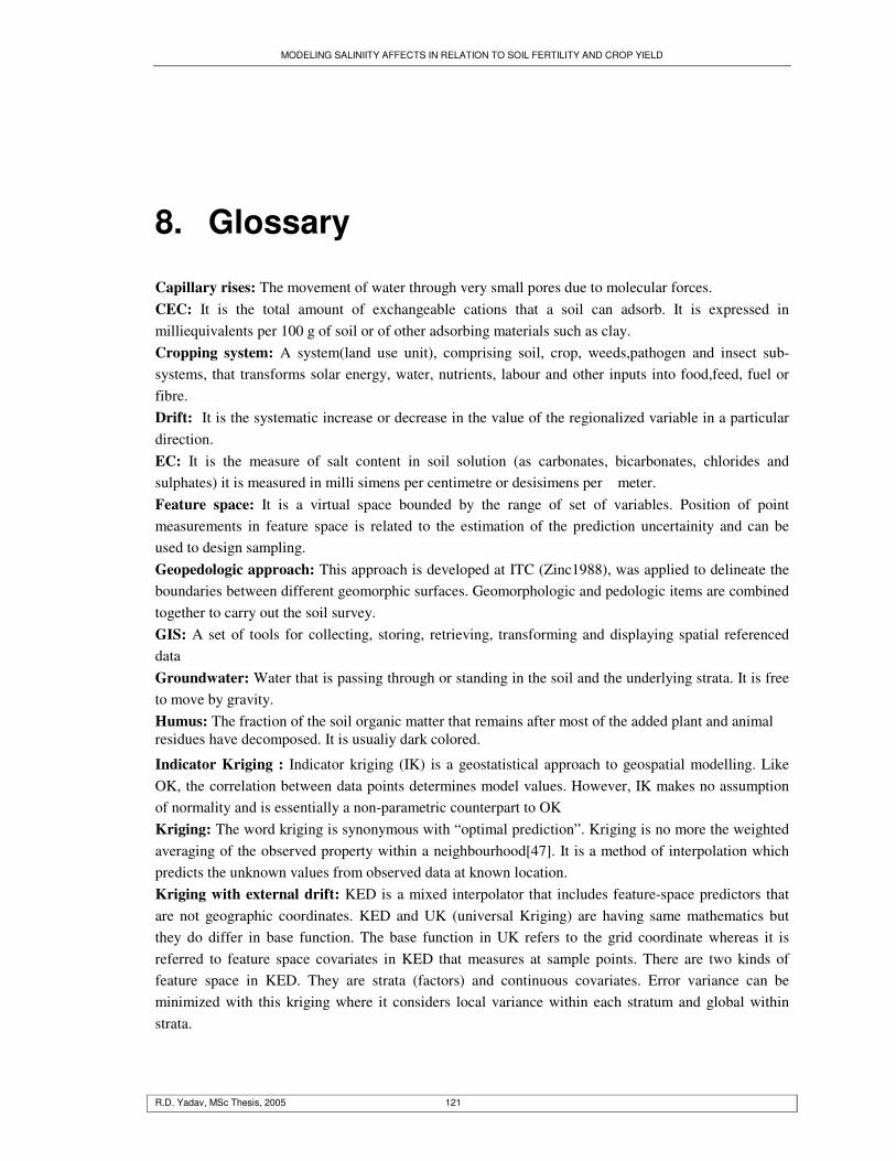
MODELING SALINIITY AFFECTS IN RELATION TO SOIL FERTILITY AND CROP YIELD
R.D. Yadav, MSc Thesis, 2005 121
8. Glossary
Capillary rises: The movement of water through very small pores due to molecular forces. CEC: It is the total amount of exchangeable cations that a soil can adsorb. It is expressed in milliequivalents per 100 g of soil or of other adsorbing materials such as clay. Cropping system: A system(land use unit), comprising soil, crop, weeds,pathogen and insect sub-systems, that transforms solar energy, water, nutrients, labour and other inputs into food,feed, fuel or fibre. Drift: It is the systematic increase or decrease in the value of the regionalized variable in a particular direction. EC: It is the measure of salt content in soil solution (as carbonates, bicarbonates, chlorides and sulphates) it is measured in milli simens per centimetre or desisimens per meter. Feature space: It is a virtual space bounded by the range of set of variables. Position of point measurements in feature space is related to the estimation of the prediction uncertainity and can be used to design sampling. Geopedologic approach: This approach is developed at ITC (Zinc1988), was applied to delineate the boundaries between different geomorphic surfaces. Geomorphologic and pedologic items are combined together to carry out the soil survey. GIS: A set of tools for collecting, storing, retrieving, transforming and displaying spatial referenced data Groundwater: Water that is passing through or standing in the soil and the underlying strata. It is free to move by gravity. Humus: The fraction of the soil organic matter that remains after most of the added plant and animal residues have decomposed. It is usualiy dark colored.
Indicator Kriging : Indicator kriging (IK) is a geostatistical approach to geospatial modelling. Like OK, the correlation between data points determines model values. However, IK makes no assumption of normality and is essentially a non-parametric counterpart to OK Kriging: The word kriging is synonymous with “optimal prediction”. Kriging is no more the weighted averaging of the observed property within a neighbourhood[47]. It is a method of interpolation which predicts the unknown values from observed data at known location. Kriging with external drift: KED is a mixed interpolator that includes feature-space predictors that are not geographic coordinates. KED and UK (universal Kriging) are having same mathematics but they do differ in base function. The base function in UK refers to the grid coordinate whereas it is referred to feature space covariates in KED that measures at sample points. There are two kinds of feature space in KED. They are strata (factors) and continuous covariates. Error variance can be minimized with this kriging where it considers local variance within each stratum and global within strata.

MODELING SALINIITY AFFECTS IN RELATION TO SOIL FERTILITY AND CROP YIELD
R.D. Yadav, MSc Thesis, 2005 122
Landform: The various shapes of.the land surface resulting from a variety of actions such as deposition or sedimentation (eskers, lacustrine basins), erosion (gullies, canyons), and earth crust movements (mountains). Landform = topographic form + geomorphic position + geomorphic unit = Soil formation frame Landscape: All the natural features such as fields, hills, forests, and water that distinguish one part of the earth's surface from another part. Usually it is the portion of land or territory that the eye can see in a single view, including all its natural characteristics. (e.g. peneplain, valley). Metric potential: The amount of work that must be done per unit quantity of pure water in order to transport reversibly and isothermally an infinitesimal quantity of water, identical in composition with the soil water, from a pool at the elevation and the external gas pressure of the point under consideration, to the soil water. Moving Average: Moving average (inverse distance) is local estimator, calculate the arithmetic average for a central point within a predefined neighbourhood (i.e. moving window with a certain limiting distance). It assumes that each input point has a local influence that diminishes with the distance. It givesweights the points closer to the processing cell greater than those farther away. Nugget Effect: “Though the value of the variogram for h=0 is strictly 0, several factors, such as sampling error and short scale variability may cause sample values separated by extremely small distances to be quite dissimilar. This causes a discontinuity at the origin to the value of the variogram. The vertical jump from the value of 0 at the origin to the value of variogram at extremely small separation distance is called nugget effect”. It is denoted by C0 Ordinary kriging (OK): OK is a geostatistical approach to modeling. Instead of weighting nearby data points by some power of their inverted distance, OK relies on the spatial correlation structure of the data to determine the weighting values. This is a more rigorous approach to modeling, as correlation between data points determines the estimated value at an unsampled point. Organic matter: It is the organic fraction of soil. Organic matter of the soil arises from the debries of green plants,animal residues and excreta that are deposited on the surface and mixed to a variable extent with the mineral component. Osmotic potential: The amount of work that must be done per unit quantity of pure water in order to transport reversibly and isothermally an infinitesimal quantity of water from a pool of pure water, at a specified elevation and at atmospheric pressure, to a pool of water identical in composition with the soil water at the point under consideration, but in all other respects being identical with the reference pool. Parcel: A contiguous piece of land with uniform tenure and physical characteristics. A parcel may consist of one or more plots adjacent to each other Peneplain: A rugged area that was high at one time, but has been reduced by erosion to a low, gently rolling surface resembling a plain. Physical properties of soil: The characteristics, processes, or reactions of a soil that are caused by physical forces, and are described by, or expressed in, physical terms or equations. Sometimes physical properties are confused with and hard to separate from chemical properties; hence, the terms "physical-chemical" or "physicochemical." Examples of physical properties are bulk density, water-holding capacity, hydraulic conductivity, porosity, and pore-size distribution. Piezometric surface: The surface at which water will stand in a series of piezometers Range: As the separation distance of two pairs increase, the variogram value of those two pairs also generally increases. Eventually, an increase in separation distance no longer causes to increase the
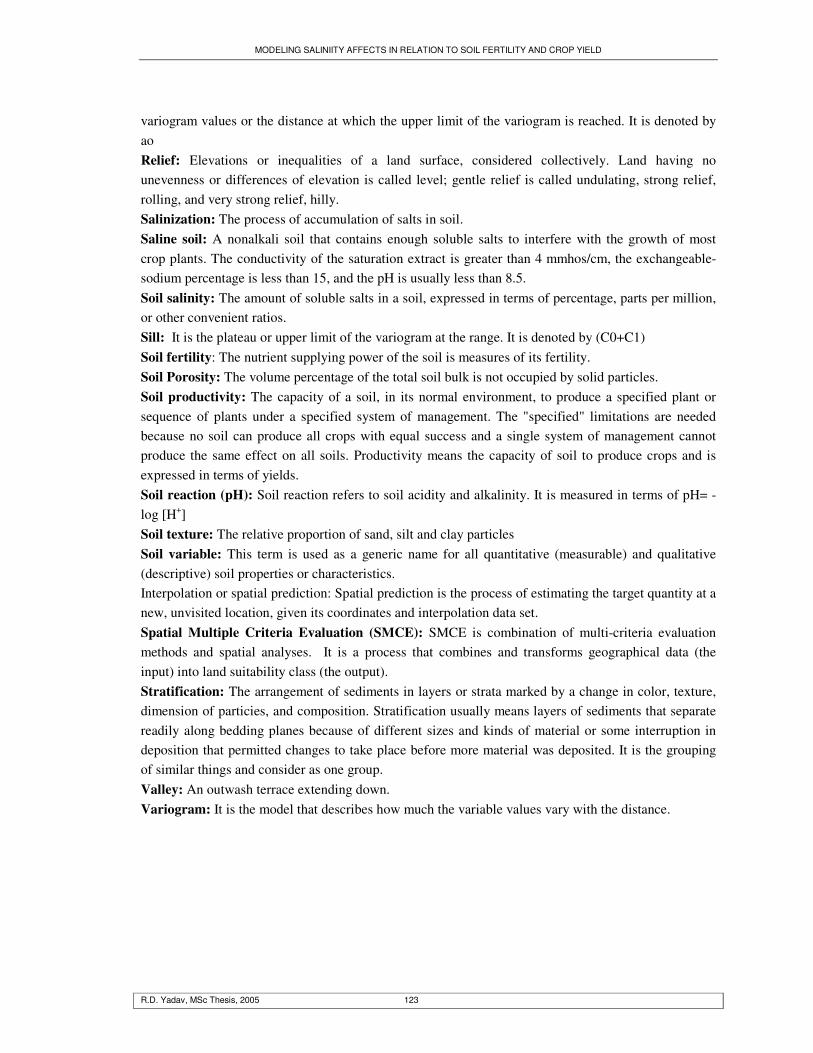
MODELING SALINIITY AFFECTS IN RELATION TO SOIL FERTILITY AND CROP YIELD
R.D. Yadav, MSc Thesis, 2005 123
variogram values or the distance at which the upper limit of the variogram is reached. It is denoted by ao Relief: Elevations or inequalities of a land surface, considered collectively. Land having no unevenness or differences of elevation is called level; gentle relief is called undulating, strong relief, rolling, and very strong relief, hilly. Salinization: The process of accumulation of salts in soil. Saline soil: A nonalkali soil that contains enough soluble salts to interfere with the growth of most crop plants. The conductivity of the saturation extract is greater than 4 mmhos/cm, the exchangeable-sodium percentage is less than 15, and the pH is usually less than 8.5. Soil salinity: The amount of soluble salts in a soil, expressed in terms of percentage, parts per million, or other convenient ratios. Sill: It is the plateau or upper limit of the variogram at the range. It is denoted by (C0+C1) Soil fertility: The nutrient supplying power of the soil is measures of its fertility. Soil Porosity: The volume percentage of the total soil bulk is not occupied by solid particles. Soil productivity: The capacity of a soil, in its normal environment, to produce a specified plant or sequence of plants under a specified system of management. The "specified" limitations are needed because no soil can produce all crops with equal success and a single system of management cannot produce the same effect on all soils. Productivity means the capacity of soil to produce crops and is expressed in terms of yields. Soil reaction (pH): Soil reaction refers to soil acidity and alkalinity. It is measured in terms of pH= -log [H+] Soil texture: The relative proportion of sand, silt and clay particles Soil variable: This term is used as a generic name for all quantitative (measurable) and qualitative (descriptive) soil properties or characteristics. Interpolation or spatial prediction: Spatial prediction is the process of estimating the target quantity at a new, unvisited location, given its coordinates and interpolation data set. Spatial Multiple Criteria Evaluation (SMCE): SMCE is combination of multi-criteria evaluation methods and spatial analyses. It is a process that combines and transforms geographical data (the input) into land suitability class (the output). Stratification: The arrangement of sediments in layers or strata marked by a change in color, texture, dimension of particies, and composition. Stratification usually means layers of sediments that separate readily along bedding planes because of different sizes and kinds of material or some interruption in deposition that permitted changes to take place before more material was deposited. It is the grouping of similar things and consider as one group. Valley: An outwash terrace extending down. Variogram: It is the model that describes how much the variable values vary with the distance.

MODELING SALINIITY AFFECTS IN RELATION TO SOIL FERTILITY AND CROP YIELD
R.D. Yadav, MSc Thesis, 2005 124
9. Appendices
Appendix 1: Questionnaire of household survey Date of interview:…../……./04
A. General
1. Household Number/name/village name: Coordinate: X Y 2. Field location in the study area : 3. Land holding ……rai(a) …...........rai upland (b)……………rai(low land) 4. Number of crops in a year (a)1 (b) 2 (c) 3
B. Crop 1. Cropping system (a) Maize-soyabean (b)Rice-maize (c)Maize – Cassava (d) others: 2.Crops grown and time to get yield
Yield Kg/rai
Crops Planting date
Moisture
content
Germination time (days)
Dev. stage (days)
Flowering (days)
Maturity (days)
Harvesting date
Area (rai)
grain
biomass
3.What you do with the residue (a) Animal feed (b) Leave in the field (c) Compost materials (d) others C. Management practices 1.Land preparation
Time of ploughing
Number of plough
Implement type Organic manure and amount
Mixing percentage of residue
2.Fertilizers application
crops Urea (kg/rai) DAP (kg/rai)
MoP (kg/rai)
FYM (mt/rai)
Compost (mt/rai)
Green manure
Poultry Manure
Others

MODELING SALINIITY AFFECTS IN RELATION TO SOIL FERTILITY AND CROP YIELD
R.D. Yadav, MSc Thesis, 2005 125
3.Time of fertilizer application
Fertilizer type Basal application
...days after germination
...days after first application
...days after second
application
...days after 3rd
application Urea (kg/rai)
DAP(kg/rai)
MoP(kg/rai)
Organic manure(mt/rai)
4. Irrigation schedule
Number of irrigation Amount (mm) Crops ...days after
germination(I) ...days after
1st application ( II)
...days after 2 nd application(III)
...days after 3rd application(IV)
I II III IV
5. Pesticides
Types of chemicals
Stages of maize Stages of soyabean
Concentration (ml/lit)
Total amount (Lit/rye)
6. Distance of field from home
Field Number/name) Coordinate Distance(km)
7. Labour Fertilization Operation Land
preparation
Chemical Manure
Irrigation Pesticide application
Inter-cultivation
Harvesting
Threshing
Cost /
labour
Number of
labour

MODELING SALINIITY AFFECTS IN RELATION TO SOIL FERTILITY AND CROP YIELD
R.D. Yadav, MSc Thesis, 2005 126
8. Livestock Animal type Age Number Type of Feed Feed Amount
Buffaloes
Cows
OX
Swine/pig
Poultry
9. What do you think in yield in last 10 years? (a) Increased ……….. (b) Decreased ………..(c)No change 10. If decreased then what will be the cause. (a) Salinity (b) Not enough chemical fertilizer(c) Not enough manure 11. Have you tested your soil? (a) Yes (b) No 12. What were your analysis result and what management you practiced? (a) Apply fertilizer ………………kg/rai.(b) Apply Manure……………ton(c)Irrigate land
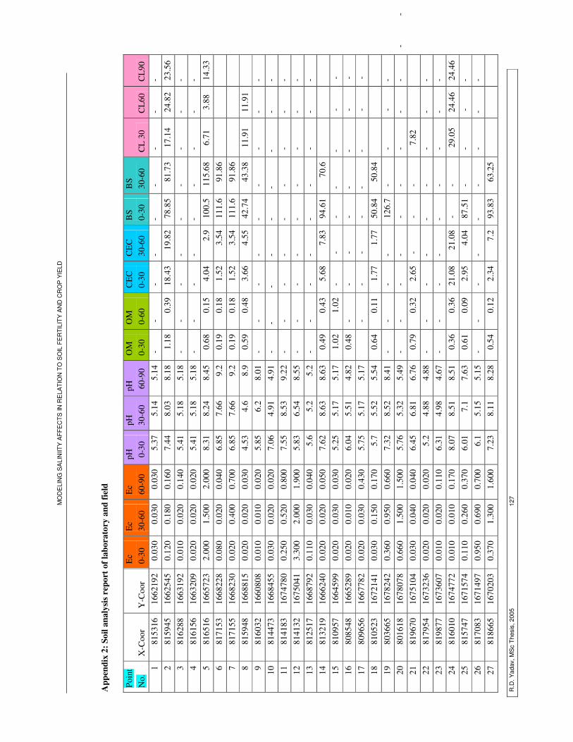
MO
DE
LIN
G S
ALI
NIIT
Y A
FFE
CT
S IN
RE
LAT
ION
TO
SO
IL F
ER
TILI
TY
AN
D C
RO
P Y
IELD
R.D
. Yad
av, M
Sc
The
sis,
200
5 12
7
App
endi
x 2:
Soi
l ana
lysi
s rep
ort o
f lab
orat
ory
and
field
Po
int
No.
X
-Coo
r Y
-Coo
r E
c
0-30
E
c
30
-60
Ec
60
-90
pH
0-3
0 pH
30
-60
pH
6
0-90
O
M
0-30
O
M
0-60
C
EC
0-30
C
EC
30
-60
BS
0-
30
BS
30
-60
CL
30
CL6
0 C
L90
1 81
5316
16
6219
2 0.
030
0.03
0 0.
030
5.37
5.
14
5.14
-
- -
- -
- -
- -
2 81
5945
16
6254
5 0.
120
0.18
0 0.
160
7.44
8.
03
8.18
1.
18
0.39
18
.43
19.8
2 78
.85
81.7
3 17
.14
24.8
2 23
.56
3 81
6288
16
6319
2 0.
010
0.02
0 0.
140
5.41
5.
18
5.18
-
- -
- -
- -
- -
4 81
6156
16
6320
9 0.
020
0.02
0 0.
020
5.41
5.
18
5.18
-
- -
- -
- -
- -
5 81
6516
16
6572
3 2.
000
1.50
0 2.
000
8.31
8.
24
8.45
0.
68
0.15
4.
04
2.9
100.
5 11
5.68
6.
71
3.88
14
.33
6 81
7153
16
6822
8 0.
080
0.02
0 0.
040
6.85
7.
66
9.2
0.19
0.
18
1.52
3.
54
111.
6 91
.86
7
8171
55
1668
230
0.02
0 0.
400
0.70
0 6.
85
7.66
9.
2 0.
19
0.18
1.
52
3.54
11
1.6
91.8
6
8 81
5948
16
6881
5 0.
020
0.02
0 0.
030
4.53
4.
6 8.
9 0.
59
0.48
3.
66
4.55
42
.74
43.3
8 11
.91
11.9
1
9 81
6032
16
6080
8 0.
010
0.01
0 0.
020
5.85
6.
2 8.
01
- -
- -
- -
- -
- 10
81
4473
16
6845
5 0.
030
0.02
0 0.
020
7.06
4.
91
4.91
-
- -
- -
- -
- -
11
8141
83
1674
780
0.25
0 0.
520
0.80
0 7.
55
8.53
9.
22
- -
- -
- -
- -
- 12
81
4132
16
7504
1 3.
300
2.00
0 1.
900
5.83
6.
54
8.55
-
- -
- -
- -
- -
13
8125
17
1668
792
0.11
0 0.
030
0.04
0 5.
6 5.
2 5.
2 -
- -
- -
- -
- -
14
8132
19
1666
240
0.02
0 0.
020
0.05
0 7.
62
8.63
8.
63
0.49
0.
43
5.68
7.
83
94.6
1 70
.6
15
81
0957
16
6459
9 0.
020
0.03
0 0.
030
5.25
5.
17
5.17
1.
02
1.02
-
- -
- -
- -
16
8085
48
1665
289
0.02
0 0.
010
0.02
0 6.
04
5.51
4.
82
0.48
-
- -
- -
- -
- 17
80
9656
16
6778
2 0.
020
0.03
0 0.
430
5.75
5.
17
5.17
- -
- -
- -
- -
18
8105
23
1672
141
0.03
0 0.
150
0.17
0 5.
7 5.
52
5.54
0.
64
0.11
1.
77
1.77
50
.84
50.8
4
19
8036
65
1678
242
0.36
0 0.
950
0.66
0 7.
32
8.52
8.
41
- -
- -
126.
7 -
- -
- 20
80
1618
16
7807
8 0.
660
1.50
0 1.
500
5.76
5.
32
5.49
-
- -
- -
- -
- -
- -
21
8196
70
1675
104
0.03
0 0.
040
0.04
0 6.
45
6.81
6.
76
0.79
0.
32
2.65
-
- -
7.82
22
81
7954
16
7323
6 0.
020
0.02
0 0.
020
5.2
4.88
4.
88
- -
- -
- -
- -
- 23
81
9877
16
7360
7 0.
010
0.02
0 0.
110
6.31
4.
98
4.67
-
- -
- -
- -
- -
24
8160
10
1674
772
0.01
0 0.
010
0.17
0 8.
07
8.51
8.
51
0.36
0.
36
21.0
8 21
.08
- -
29.0
5 24
.46
24.4
6 25
81
5747
16
7157
4 0.
110
0.26
0 0.
370
6.01
7.
1 7.
63
0.61
0.
09
2.95
4.
04
87.5
1 -
- -
- 26
81
7083
16
7149
7 0.
950
0.69
0 0.
700
6.1
5.15
5.
15
- -
- -
- -
- -
- 27
81
8665
16
7020
3 0.
370
1.30
0 1.
600
7.23
8.
11
8.28
0.
54
0.12
2.
34
7.2
93.8
3 63
.25

MO
DE
LIN
G S
ALI
NIIT
Y A
FFE
CT
S IN
RE
LAT
ION
TO
SO
IL F
ER
TILI
TY
AN
D C
RO
P Y
IELD
R.D
. Yad
av, M
Sc
The
sis,
200
5 12
8
28
8091
96
1674
661
0.22
0 0.
550
0.70
0 6.
2 6.
3 8.
2 0.
81
0.06
6.
44
13.3
8 71
.39
74.1
7 9.
44
19.1
7 23
.39
29
8067
93
1673
956
0.02
0 0.
020
0.03
0 5.
91
6.21
6.
75
- -
- -
- -
- -
- 30
80
5033
16
7189
2 0.
020
0.08
0 0.
050
5.91
5.
03
4.93
-
- -
- -
- -
- -
31
8085
99
1672
631
0.02
0 0.
020
0.02
0 6.
06
4.9
5.03
0.
23
0.08
1.
89
2.02
14
2.7
109.
75
13.0
4 8.
89
8.89
32
81
2841
16
7252
7 0.
020
0.03
0 0.
030
4.85
4.
2 4.
2 0.
4 0.
13
4.42
3.
79
25.5
31
.41
33
80
9836
16
7082
8 0.
020
0.01
0 0.
010
4.95
4.
9 4.
9 -
- -
- -
- 2.
09
- -
34
8048
96
1668
820
0.02
0 0.
010
0.04
0 5.
78
5.64
5.
55
1.13
0.
24
4.17
2.
65
65.6
5 63
.34
13.9
2 10
.81
10.8
1 35
80
6961
16
6908
3 0.
020
0.02
0 0.
020
5.86
6.
07
5.67
0.
16
- -
- -
- -
- -
36
8068
70
1665
471
0.02
0 0.
020
0.03
0 6.
37
5.08
5.
08
- -
- -
- -
- -
- 37
80
4174
16
6580
1 0.
020
0.02
0 0.
020
5.51
5.
21
5.21
-
- -
- 14
8.6
144.
96
- -
- 38
80
5724
16
6307
9 0.
030
0.02
0 0.
020
8.23
7.
75
7.32
0.
85
0.85
8.
96
5.93
20
.13
16.1
0 16
.10
39
8082
71
1662
537
0.02
0 0.
020
0.02
0 5.
2 5.
13
5.06
0.
45
0.13
8.
71
8.59
59
.39
60.9
3 19
.24
22.6
5 22
.65
40
8125
57
1663
596
0.02
0 0.
020
0.03
0 5.
46
5.01
5.
01
- -
- -
- -
- -
- 41
81
3258
16
6089
7 0.
010
0.01
0 0.
020
5.92
5.
98
5.77
-
- -
- -
- -
- -
42
8176
27
1675
366
0.01
0 0.
030
0.06
0 8.
03
8.37
8.
67
0.29
0.
42
4.92
9.
6 91
.56
104.
67
43
80
4179
16
6985
9 0.
02
0.03
5 0.
018
5.52
5.
14
5.14
0.
26
0.26
1.
89
2.25
75
.18
44.0
3 9.
84
14.3
1 14
.31
44
8049
81
1661
113
0.01
4 0.
02
0.01
6 5.
64
5.01
5.
01
0.36
0.
37
3.54
3.
79
59.2
4 43
.64
12.9
5 19
.85
45
80
4366
16
6359
6 0.
038
0.02
0.
022
5.12
4.
86
4.82
-
- -
- -
- -
- -
46
8045
04
1666
705
0.02
6 0.
061
0.06
1 5.
86
5.86
6.
08
- -
- -
- -
- -
- 47
80
7495
16
5770
3 0.
066
0.08
8 0.
067
8.15
8.
1 8.
2 0.
89
0.75
22
.47
20.5
8 10
9.9
199.
47
49.1
9 48
.18
48.1
8 48
80
9347
16
5770
3 0.
026
0.03
6 0.
034
6.44
5.
26
5.05
0.
45
0.37
5.
3 9.
09
116.
8 53
.9
11.5
0 26
.95
26.9
5 49
81
8557
16
5624
3 0.
006
0.02
5 0.
024
5.86
5.
3 5.
21
0.66
0.
9 2.
78
3.66
77
.42
93.1
7.
05
13.0
4 13
.04
50
8167
91
1661
316
0.02
1 0.
035
0.02
7 5.
49
5.56
5.
3 -
- -
- -
- -
- -
51
8185
40
1672
340
4.00
0 0.
66
0.8
8.57
8.
75
8.8
0.27
0.
24
4.5
6.19
12
1.9
74.5
2 -
- -
52
8041
37
1673
100
0.02
0.
024
0.02
5 5.
53
5.1
4.96
0.
46
0.45
2.
02
2.65
57
.81
31
- -
- 53
80
7338
16
7469
5 0.
02
0.02
0.
015
4.96
5.
12
5.06
0.
62
0.49
2.
15
3.41
53
.33
54.1
2 6.
33
8.89
8.
89
54
8174
79
1674
121
0.07
6 0.
18
0.18
8.
42
9.18
9.
18
0.88
0.
55
- -
- -
- -
- 55
81
0965
16
5774
2 0.
094
0.07
6 0.
065
8.11
8.
37
8.45
2.
45
1.8
43.1
8 9.
09
63.4
8 30
3.7
43.4
8 46
.73
45.5
8 56
80
5838
16
5951
0 0.
077
0.07
2 0.
16
7.05
7.
85
8.73
0.
94
0.48
-
- -
- -
- -
57
8150
25
1658
844
0.04
6 0.
034
0.00
6 7.
24
7.1
5.92
0.
24
0.29
-
- -
- 4.
74
10.8
8 16
.27
58
8080
38
1667
174
0.01
2 0.
0054
0.
01
5.75
5.
72
5.63
-
- -
- -
- -

MO
DE
LIN
G S
ALI
NIIT
Y A
FFE
CT
S IN
RE
LAT
ION
TO
SO
IL F
ER
TILI
TY
AN
D C
RO
P Y
IELD
R.D
. Yad
av, M
Sc
The
sis,
200
5 12
9
59
8075
84
1661
415
0.01
6 0.
012
0.00
6 5.
2 5.
41
5.5
0.61
0.
62
15.0
2 4.
04
19.3
9 83
.14
- -
- 60
81
1662
16
6723
6 0.
037
0.06
0.
12
6.52
6.
94
7.21
1.
61
0.29
5.
69
4.55
90
98
.88
7.18
6.
48
61
81
0951
16
6272
2 0.
064
0.06
2 0.
062
8.29
8.
25
8.25
0.
94
0.46
-
- -
- -
- -
62
8106
69
1657
965
0.18
0.
18
0.18
8.
5 8.
5 8.
5 1.
81
1.81
21
.59
21.5
9 11
2.8
112.
81
63
80
7294
16
7060
5 0.
018
0.02
9 0.
043
6.34
6.
48
5.61
-
- -
- -
- -
- -
64
8109
31
1664
520
0.01
5 0.
015
0.01
5 -
- -
0.64
-
5.18
4.
8 86
.31
48.0
7
65
8182
18
1672
585
0.03
2 0.
036
0.03
5.
78
4.86
4.
86
- -
- -
- -
- -
- 66
80
9717
16
6490
9 0.
057
0.02
4 0.
024
6.45
5.
19
5.19
-
- -
- -
- -
- -
67
8126
22
1663
496
0.01
6 0.
01
0.01
5.
84
6.17
6.
17
- -
- -
- -
- -
- 68
81
6764
16
6139
9 0.
840
2.25
2.
25
8.02
9.
06
9.06
-
- -
- -
- -
- -
69
8132
81
1673
331
0.18
0 0.
58
0.9
9.71
9.
57
9 -
- -
- -
- -
- -
70
8107
55
1668
581
0.46
0 0.
52
0.73
10
.17
10.2
10
.2
- -
- -
- -
- -
- 71
81
0090
16
6916
6 0.
180
0.42
0.
42
8.78
10
.2
10.2
-
- -
- -
- -
- -

MODELING SALINIITY AFFECTS IN RELATION TO SOIL FERTILITY AND CROP YIELD
R.D. Yadav, MSc Thesis, 2005 130
Appendix 3: Minipit analysis data
Profile No. X-Coor Y-Coor
Soil depth
Soil pH (pH meter)
EC(1:5) µS/cm Texture Colour
Field pH (Indicator)
1 815182 1660836 0-25 5.21 8 LS 7.5YR5/4 4.8 25-70 4.97 10 SL 5YR4/6 4.5 70-85 4.87 15 SCL 5YR5/6 4.8 85-115 4.92 12 SL 5YR4/6 4.5 115-135 5.08 10 SL 5YR5/6 4.4 135-150 5.23 8 SL 5YR5/6 4.4
2 815941 1662549 0-25 8.15 100 L 10YR2/1 7.5 25-60 8.09 2600 CL 10YR3/1 7.5 60-80 7.99 3000 CL 10YR3/1 8 80-110 7.79 3400 CL 10YR5/2+7.5YR5/2 8.3 110-165 8.78 560 CL 10YR7/1+7/2 9
3 816627 1664072 0-25 6.01 12 LS 7.5YR5/4 4.8 25-60 5.64 10 LS 5YR5/6 4.6 60-110 5.3 12 SL 5YR5/8 4.5 110-160 5.15 25 SL 5YR6/8 4.4
4 816527 1665575 0-15 8.88 2600 LS 7.5YR6/4 9 15-28 9.23 2700 SL 10YR4/1+7.5YR5/3 9.2 28-40 8.88 2600 S 7.5YR5/4 9 40-50 8.66 4200 LS 10YR5/2 9.5 50-70 9.18 2800 SL 10YR6/2+7.5YR6/3 8.5 >70 Gravel
5 817062 1666815 0-27 7.31 700 LS 7.5YR5/3 7.5 27-45 7.43 600 LS 7.5YR5/4 8 45-60 8.17 800 SL 7.5YR6/3 8 60-80 8.37 880 SL 7.5YR6/4 8.5 80-100 9.4 900 SCL 7.5YR6/4 8 100-150 8.98 960 SCL 7.5YR7/4 8.5
6 808279 1659542 0-25 8.19 160 C 7.5YR3/2 7.3 25-60 8.18 160 C 7.5YR4/3 7.5 CR R
7 807936 1661672 0-9 7.05 80 L 10YR4/2 5 9 TO35 7.39 120 SCL 10YR5/3+4/1 6 35-46 7.74 100 SL 7.5YR4/3+10YR5/2 6.3 46-75 7.43 80 SL 5YR4/6 5.5 75-100 5.26 60 SL 5YR5/6 4.6 100-150 5.5 60 SL 5YR5/8 4.5
8 812952 1671931 0-20 5.87 60 LS 7.5YR5/3 4.5 20-50 6.3 80 LS 7.5YR5/3 5 50-85 5.67 70 SL 5YR5/8 4.5

MODELING SALINIITY AFFECTS IN RELATION TO SOIL FERTILITY AND CROP YIELD
R.D. Yadav, MSc Thesis, 2005 131
85-125 5.6 100 LS 7.5YR5/3 5 125-175 5.56 80 SL 5YR5/8 4.5
9 814700 1674311 0-18 6.44 240 SL 7.5YR4/2+10YR4/2 5.5 18-45 5.34 960 CL 10YR4/2 4.8 45-75 4.79 3800 SCL 10YR5/2+7.5YR5/2 4.6
75-110 7.28 3400 SCL 7.5YR6/3+7.5YR6/1 4.7
110-150 7.96 3400 SC 7.5YR6/4+7.5YR6/1 8
10 813165 1666783 O-12 9.56 140 FS 7.5YR5/3+10YR4/3 6.8 12 TO 26 9.04 540 LS 10YR3/2+7.5YR5/3 8 26-74 8.73 760 SL 10YR4/2+7.5YR5/3 6.8 74-89 9.18 670 SL 7.5YR4/3 8.5 89-104 9.61 700 LS 7.5YR5/3 8.5 104-154 9.84 80 SCL 7.5YR6/3 8
11 812503 1669274 0-25 5.86 30 LS 7.5YR4/3 4.8 25-37 6.34 34 LS 7.5YR3/2+4/4 5 37-80 6.45 24 SL 7.5YR5/6 4.5 80-150 5.31 80 SL 7.5YR6/8 4.5
12 809439 1674646 0-7 8.23 760 L 10YR3/2 8 7 TO 34 8.63 2600 SL 10YR5/3 8 34-46 8.85 920 SL 7.5YR6/4 8.5 46-66 8.71 2000 SCL 7.5YR7/3+6/3 8.7 66-106 8.83 1800 CL 7.5YR7/4 8.5 106-131 8.93 1800 CL 7.5YR6/4 8 131-176 8.71 1600 CL 10YR7/3 8.5
13 807447 1674500 0-20 6.36 20 FS 10YR4/2 5.5 20-36 6.84 14 LS 7.5YR6/4+3/2 5.5 36-48 6.75 16 SL 5YR5/6+7.5YR3/2 4.5 48-95 6.36 40 SL 7.5YR5/4 5.8 95-110 7.62 100 SL 5YR5/3+6/2 6.5 110-150 9.01 200 SCL 7.5YR6/4 8.5
14 808498 1656345 0-22 7.83 46 CL 7.5YR3/2 7 22-50 6.89 50 C 7.5YR3/3 5.8 50-80 8.01 120 C 7.5YR4/4 4.5
>80 7.52 640 FRAG.ROCK 8
15 810743 1657985 0-24 8.43 70 CL 10YR3/2 7.5 24-34 8.47 92 SGCL 7.5YR4/3 7.5 34-50 8.5 120 GCL 7.5YR4/4 8 50-80+ 8.66 120 VGLS 9
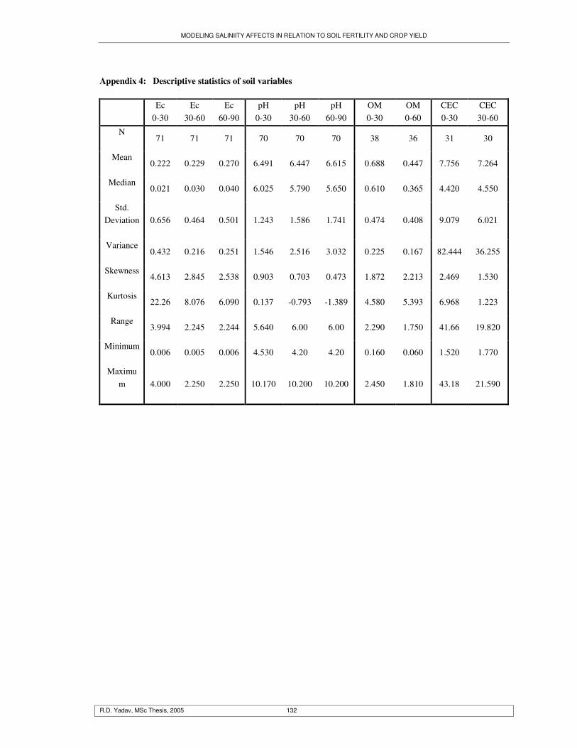
MODELING SALINIITY AFFECTS IN RELATION TO SOIL FERTILITY AND CROP YIELD
R.D. Yadav, MSc Thesis, 2005 132
Appendix 4: Descriptive statistics of soil variables
Ec
0-30 Ec
30-60 Ec
60-90 pH
0-30 pH
30-60 pH
60-90 OM 0-30
OM 0-60
CEC 0-30
CEC 30-60
N
71 71 71 70 70 70 38 36 31 30
Mean
0.222 0.229 0.270 6.491 6.447 6.615 0.688 0.447 7.756 7.264
Median
0.021 0.030 0.040 6.025 5.790 5.650 0.610 0.365 4.420 4.550
Std. Deviation
0.656 0.464 0.501 1.243 1.586 1.741 0.474 0.408 9.079 6.021
Variance
0.432 0.216 0.251 1.546 2.516 3.032 0.225 0.167 82.444 36.255
Skewness
4.613 2.845 2.538 0.903 0.703 0.473 1.872 2.213 2.469 1.530
Kurtosis
22.26 8.076 6.090 0.137 -0.793 -1.389 4.580 5.393 6.968 1.223
Range
3.994 2.245 2.244 5.640 6.00 6.00 2.290 1.750 41.66 19.820
Minimum
0.006 0.005 0.006 4.530 4.20 4.20 0.160 0.060 1.520 1.770
Maximum
4.000 2.250 2.250 10.170 10.200 10.200 2.450 1.810 43.18 21.590
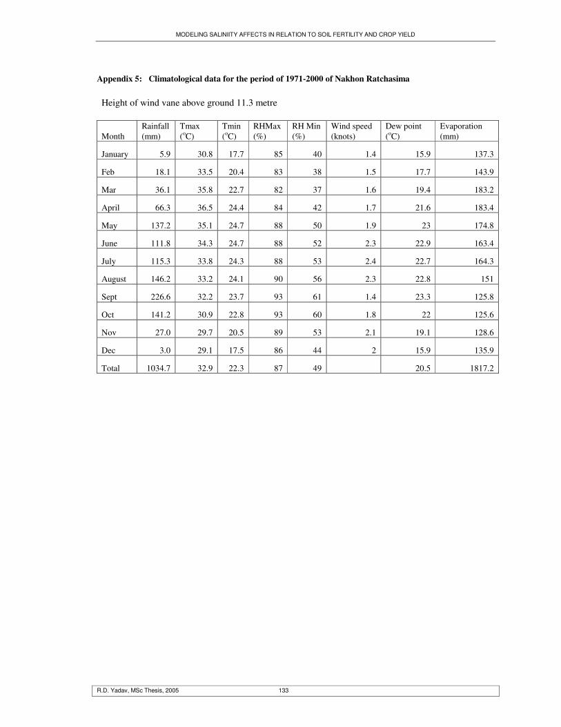
MODELING SALINIITY AFFECTS IN RELATION TO SOIL FERTILITY AND CROP YIELD
R.D. Yadav, MSc Thesis, 2005 133
Appendix 5: Climatological data for the period of 1971-2000 of Nakhon Ratchasima Height of wind vane above ground 11.3 metre
Month Rainfall (mm)
Tmax (oC)
Tmin (oC)
RHMax (%)
RH Min (%)
Wind speed (knots)
Dew point (oC)
Evaporation (mm)
January 5.9 30.8 17.7 85 40 1.4 15.9 137.3
Feb 18.1 33.5 20.4 83 38 1.5 17.7 143.9
Mar 36.1 35.8 22.7 82 37 1.6 19.4 183.2
April 66.3 36.5 24.4 84 42 1.7 21.6 183.4
May 137.2 35.1 24.7 88 50 1.9 23 174.8
June 111.8 34.3 24.7 88 52 2.3 22.9 163.4
July 115.3 33.8 24.3 88 53 2.4 22.7 164.3
August 146.2 33.2 24.1 90 56 2.3 22.8 151
Sept 226.6 32.2 23.7 93 61 1.4 23.3 125.8
Oct 141.2 30.9 22.8 93 60 1.8 22 125.6
Nov 27.0 29.7 20.5 89 53 2.1 19.1 128.6
Dec 3.0 29.1 17.5 86 44 2 15.9 135.9
Total 1034.7 32.9 22.3 87 49 20.5 1817.2
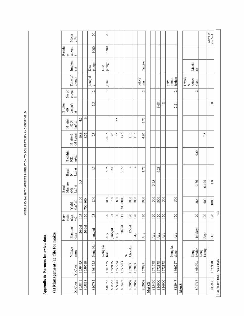
MO
DE
LIN
G S
ALI
NIIT
Y A
FFE
CT
S IN
RE
LAT
ION
TO
SO
IL F
ER
TILI
TY
AN
D C
RO
P Y
IELD
R.D
. Yad
av, M
Sc
The
sis,
200
5 13
4
App
endi
x 6:
Far
mer
s Int
ervi
ew d
ata
(a) M
anag
emen
t (1)
file
for
mai
ze
X_C
oor
Y_C
oor
Vill
age
nam
e Pl
antin
g da
te
Har
ves
ting(
days
) Y
ield
(k
g/ra
i)
Bas
al
Man
ure
(N)
kg/r
ai
Bas
al
N
kg/r
ai
N w
ithin
30
D
kg/r
ai
N_a
fter
30d
kg/
rai
N_a
fter
_45D
kg
/rai
N_a
fter
_60
dayk
g/r
ai
No
of
plou
gh
Ti
me
of
plou
gh
Impl
emen
t
Res
idu
e amou
nt
Mix
ing
%
8058
41
1659
445
26
-Jul
10
5 11
00
0.5
16.8
4.
5
80
5838
16
5951
0
20-J
ul
120
700-
800
8.
52
6
8107
82
1661
525
Non
g H
oi
june
/jul
95
800
1.
5
23
2.
5 2
june
/jul
y D
isc
plou
gh
1000
70
8107
82
1661
525
Non
g Sa
K
ae
July
90
10
00
3.
75
26
.75
3 ju
ne
Dis
c pl
ough
35
00
70
8083
82
1659
125
ju
ne/ju
l 95
70
0
2.1
23
8093
47
1657
224
Ju
ly
90
800
7.
5 7.
5
80
7495
16
5770
3
20-J
ul
115
700-
800
2.
72
13
.5
8020
68
1678
891
Sa
Cho
rake
12
-Jul
12
0 10
00
4
11
.5
80
2068
16
7889
1
july
12
0 10
00
4
11
.5
8020
68
1678
891
Ju
ly
120
1000
2.72
4.95
2.
72
2
befo
re
rain
T
ract
or
Mgt
(2)
81
5470
16
7167
8
Aug
12
0 50
0 3.
75
8169
00
1672
178
A
ug
120
1000
6.28
9.68
8169
00
1672
178
A
ug
120
500
8
8129
47
1666
227
Non
g ka
do
ne
Aug
12
0 50
0
2.21
2
prev
m
onth
&pl
ant
Mgt
(3)
8017
17
1664
903
Non
g kr
adon
1s
t Sep
t 70
28
6 3.
36
9.
66
2
1 w
eek
&
befo
re
plan
t M
achi
ne
Non
g Lu
ang
Sept
12
0 50
0 0.
125
7.5
8159
70
1672
178
O
ct
120
1000
1.
8
8
Lea
ve in
th
e fi
eld
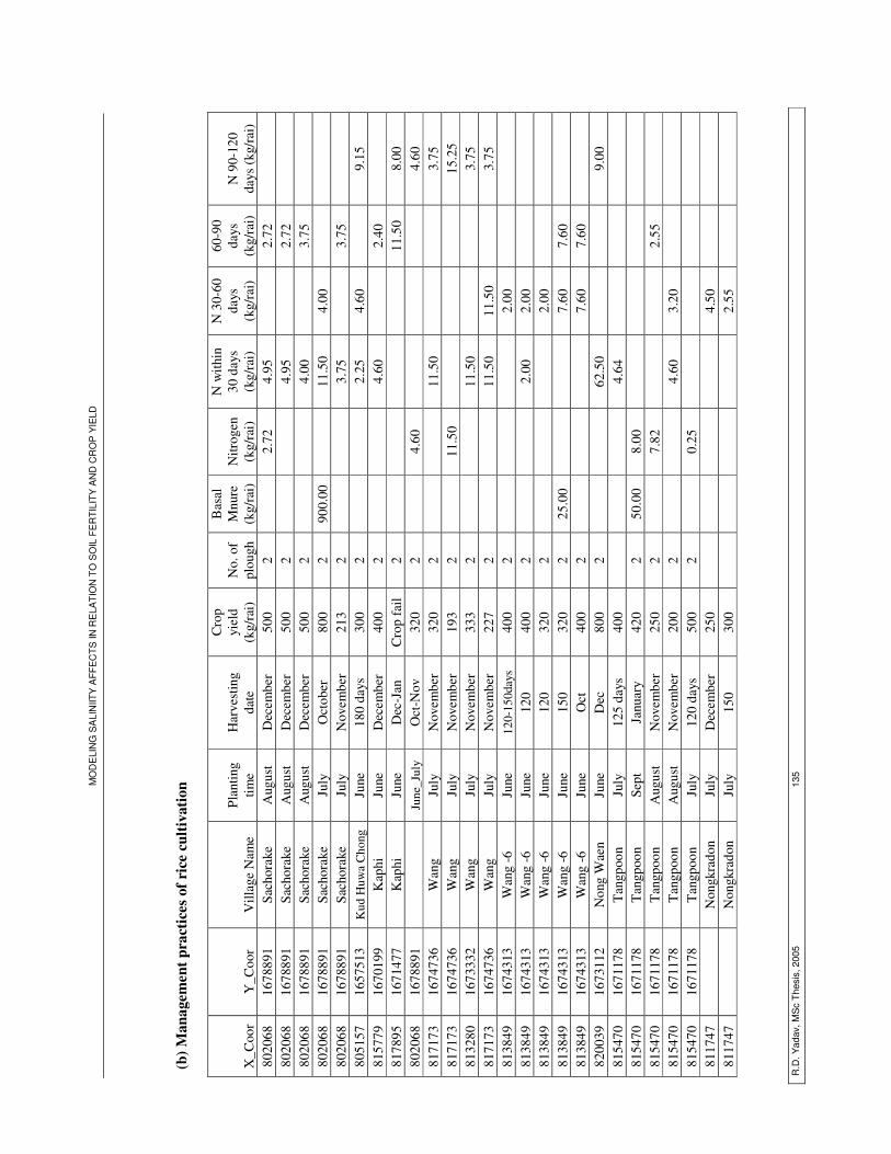
MO
DE
LIN
G S
ALI
NIIT
Y A
FFE
CT
S IN
RE
LAT
ION
TO
SO
IL F
ER
TILI
TY
AN
D C
RO
P Y
IELD
R.D
. Yad
av, M
Sc
The
sis,
200
5 13
5
(b) M
anag
emen
t pra
ctic
es o
f ric
e cu
ltiva
tion
X_C
oor
Y_C
oor
Vill
age
Nam
e Pl
antin
g tim
e H
arve
stin
g da
te
Cro
p yi
eld
(kg/
rai)
N
o. o
f pl
ough
Bas
al
Mnu
re
(kg/
rai)
N
itrog
en
(kg/
rai)
N w
ithin
30
day
s (k
g/ra
i)
N 3
0-60
da
ys
(kg/
rai)
60-9
0 da
ys
(kg/
rai)
N
90-
120
days
(kg/
rai)
80
2068
16
7889
1 Sa
chor
ake
Aug
ust
Dec
embe
r 50
0 2
2.
72
4.95
2.72
8020
68
1678
891
Sach
orak
e A
ugus
t D
ecem
ber
500
2
4.
95
2.
72
80
2068
16
7889
1 Sa
chor
ake
Aug
ust
Dec
embe
r 50
0 2
4.00
3.75
8020
68
1678
891
Sach
orak
e Ju
ly
Oct
ober
80
0 2
900.
00
11
.50
4.00
80
2068
16
7889
1 Sa
chor
ake
July
N
ovem
ber
213
2
3.
75
3.
75
80
5157
16
5751
3 K
ud H
uwa
Cho
ng
June
18
0 da
ys
300
2
2.
25
4.60
9.15
81
5779
16
7019
9 K
aphi
Ju
ne
Dec
embe
r 40
0 2
4.60
2.40
8178
95
1671
477
Kap
hi
June
D
ec-J
an
Cro
p fa
il 2
11.5
0 8.
00
8020
68
1678
891
Ju
ne_J
uly
Oct
-Nov
32
0 2
4.
60
4.
60
8171
73
1674
736
Wan
g Ju
ly
Nov
embe
r 32
0 2
11.5
0
3.
75
8171
73
1674
736
Wan
g Ju
ly
Nov
embe
r 19
3 2
11
.50
15
.25
8132
80
1673
332
Wan
g Ju
ly
Nov
embe
r 33
3 2
11.5
0
3.
75
8171
73
1674
736
Wan
g Ju
ly
Nov
embe
r 22
7 2
11.5
0 11
.50
3.
75
8138
49
1674
313
Wan
g -6
Ju
ne
120-
150d
ays
400
2
2.00
81
3849
16
7431
3 W
ang
-6
June
12
0 40
0 2
2.00
2.
00
8138
49
1674
313
Wan
g -6
Ju
ne
120
320
2
2.00
81
3849
16
7431
3 W
ang
-6
June
15
0 32
0 2
25.0
0
7.
60
7.60
8138
49
1674
313
Wan
g -6
Ju
ne
Oct
40
0 2
7.
60
7.60
8200
39
1673
112
Non
g W
aen
June
D
ec
800
2
62
.50
9.00
81
5470
16
7117
8 T
angp
oon
July
12
5 da
ys
400
4.
64
81
5470
16
7117
8 T
angp
oon
Sept
Ja
nuar
y 42
0 2
50.0
0 8.
00
8154
70
1671
178
Tan
gpoo
n A
ugus
t N
ovem
ber
250
2
7.82
2.
55
81
5470
16
7117
8 T
angp
oon
Aug
ust
Nov
embe
r 20
0 2
4.60
3.
20
8154
70
1671
178
Tan
gpoo
n Ju
ly
120
days
50
0 2
0.
25
8117
47
N
ongk
rado
n Ju
ly
Dec
embe
r 25
0
4.
50
8117
47
N
ongk
rado
n Ju
ly
150
300
2.55
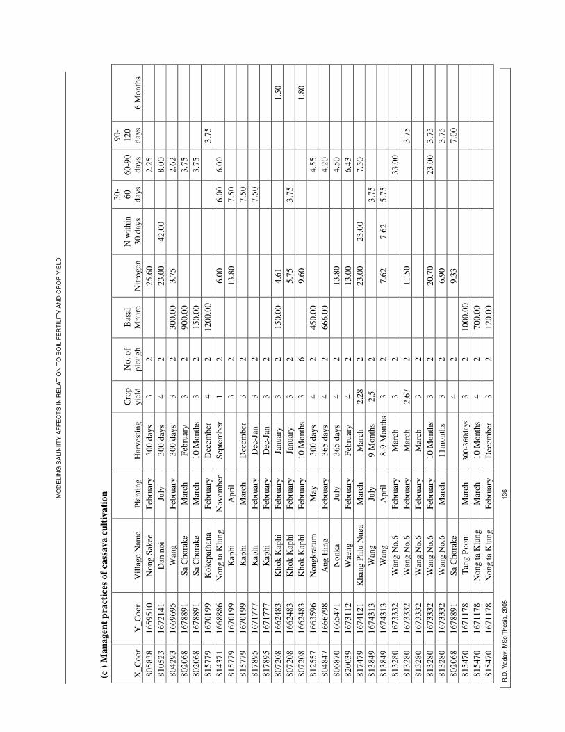
MO
DE
LIN
G S
ALI
NIIT
Y A
FFE
CT
S IN
RE
LAT
ION
TO
SO
IL F
ER
TILI
TY
AN
D C
RO
P Y
IELD
R.D
. Yad
av, M
Sc
The
sis,
200
5 13
6
(c )
Man
agen
t pra
ctic
es o
f cas
sava
cul
tivat
ion
X_C
oor
Y_C
oor
Vill
age
Nam
e Pl
antin
g H
arve
stin
g C
rop
yiel
d N
o. o
f pl
ough
B
asal
M
nure
N
itrog
en
N w
ithin
30
day
s
30-
60
days
60
-90
days
90-
120
days
6
Mon
ths
8058
38
1659
510
Non
g Sa
kee
Febr
uary
30
0 da
ys
3 2
25
.60
2.25
81
0523
16
7214
1 D
an n
oi
July
30
0 da
ys
4 2
23
.00
42.0
0
8.00
80
4293
16
6969
5 W
ang
Febr
uary
30
0 da
ys
3 2
300.
00
3.75
2.
62
8020
68
1678
891
Sa C
hora
ke
Mar
ch
Febr
uary
3
2 90
0.00
3.75
80
2068
16
7889
1 Sa
Cho
rake
M
arch
10
Mon
ths
3 2
150.
00
3.
75
8157
79
1670
199
Kok
epat
hana
Fe
brua
ry
Dec
embe
r 4
2 12
00.0
0
3.
75
81
4371
16
6888
6 N
ong
ta K
lung
N
ovem
ber
Sept
embe
r 1
2
6.00
6.00
6.
00
8157
79
1670
199
Kap
hi
Apr
il
3 2
13
.80
7.
50
81
5779
16
7019
9 K
aphi
M
arch
D
ecem
ber
3 2
7.
50
81
7895
16
7177
7 K
aphi
Fe
brua
ry
Dec
-Jan
3
2
7.50
8178
95
1671
777
Kap
hi
Febr
uary
D
ec-J
an
3 2
80
7208
16
6248
3 K
hok
Kap
hi
Febr
uary
Ja
nuar
y 3
2 15
0.00
4.
61
1.50
80
7208
16
6248
3 K
hok
Kap
hi
Febr
uary
Ja
nuar
y 3
2
5.75
3.75
8072
08
1662
483
Kho
k K
aphi
Fe
brua
ry
10 M
onth
s 3
6
9.60
1.
80
8125
57
1663
596
Non
gkra
tum
M
ay
300
days
4
2 45
0.00
4.55
80
4847
16
6679
8 A
ng H
ing
Febr
uary
36
5 da
ys
4 2
666.
00
4.
20
8068
70
1665
471
Non
ka
July
36
5 da
ys
4 2
13
.80
4.50
82
0039
16
7311
2 W
aeng
Fe
brua
ry
Febr
uary
4
2
13.0
0
6.
43
8174
79
1674
121
Kha
ng P
hlu
Nue
a M
arch
M
arch
2.
28
2
23.0
0 23
.00
7.
50
8138
49
1674
313
Wan
g Ju
ly
9 M
onth
s 2.
5 2
3.
75
81
3849
16
7431
3 W
ang
Apr
il 8-
9 M
onth
s 3
2
7.62
7.
62
5.75
8132
80
1673
332
Wan
g N
o.6
Febr
uary
M
arch
3
2
33
.00
8132
80
1673
332
Wan
g N
o.6
Febr
uary
M
arch
2.
67
2
11.5
0
3.75
8132
80
1673
332
Wan
g N
o.6
Febr
uary
M
arch
3
2
8132
80
1673
332
Wan
g N
o.6
Febr
uary
10
Mon
ths
3 2
20
.70
23.0
0 3.
75
81
3280
16
7333
2 W
ang
No.
6 M
arch
11
mon
ths
3 2
6.
90
3.
75
80
2068
16
7889
1 Sa
Cho
rake
4
2
9.33
7.00
8154
70
1671
178
Tan
g Po
on
Mar
ch
300-
360d
ays
3 2
1000
.00
8154
70
1671
178
Non
g ta
Klu
ng
Mar
ch
10 M
onth
s 4
2 70
0.00
81
5470
16
7117
8 N
ong
ta K
lung
Fe
brua
ry
Dec
embe
r 3
2 12
0.00

MO
DE
LIN
G S
ALI
NIIT
Y A
FFE
CT
S IN
RE
LAT
ION
TO
SO
IL F
ER
TILI
TY
AN
D C
RO
P Y
IELD
R.D
. Yad
av, M
Sc
The
sis,
200
5 13
7
8154
70
1671
178
Non
g ta
Klu
ng
Febr
uary
Ja
nuar
y 4
2 25
.00
8154
70
1671
178
Non
g ta
Klu
ng
may
10
Mon
ths
4 2
81
5470
16
7117
8 N
ong
ta K
lung
Fe
brua
ry
Dec
embe
r 4
2
5.28
8154
70
1671
178
Non
g K
ha D
on
June
10
Mon
ths
4 2
1000
.00
3.75
8117
47
1665
027
Non
g K
ha D
on
June
M
ay
4 2
N
ote:
1 h
a =
6.25
rai
App
endi
x 7:
Tot
al d
ry m
ass o
f mai
ze w
ith d
iffer
ent d
egre
e of
salin
ity
Soil
unit
Soil
te
xtur
e
GW
de
pts
(c
m)
EC
w
(dS/
m)
0
dS
/m
1
dS
/m
2
dS
/m
3
dS
/m
4
dS
/m
6
dS/m
7
dS/m
8
dS
/m
9
dS
/m
10
dS/m
12
dS
/m
14
dS
/m
16
dS
/m
18
dS
/m
20
dS
/m
PE
111
SL
510
0.95
84
00
8036
78
40
7489
72
05
6742
-
12
- -
- -
- -
- PE
112
LS
320
1.50
10
461
1003
6 98
28
9444
84
99
12
- -
- -
- -
- -
- PE
113
SL
380
1.00
88
64
8435
82
72
7827
74
01
6618
-
12
- -
- -
- -
- PE
114
SL
300
0.80
98
85
9149
89
06
8747
83
25
7088
65
01
12
- -
- -
- -
- PE
115
SL
334
3.34
91
88
8617
84
06
7991
75
09
6666
-
12
- -
- -
- -
- PE
211
SL
285
1.08
98
51
9310
88
77
8624
86
00
7603
66
43
12
- -
- -
- -
- PE
211
CL
285
1.08
13
047
1258
3 12
455
1228
4 12
197
1178
6 -
1151
8 -
11
358
1122
7 11
044
1084
7 10
531
12
PE31
1 SL
27
3 0.
48
1023
5 97
15
9149
88
11
8551
79
19
7051
12
-
- -
- -
- -
PE41
1 SL
14
0 6.
85
1485
7 14
640
1430
2 13
806
1327
4 11
055
7924
22
4 -
- -
- -
- -
PE41
2 SL
17
6 3.
12
1376
9 13
300
1306
4 12
493
1172
8 10
521
9462
61
85
12
- -
- -
- -
PE41
3 SL
12
2 3.
32
1510
8 15
108
1545
7 15
447
1507
9 13
292
57
37
12
- -
- -
- -
PE51
1 SL
50
0 0.
50
8419
80
46
7829
75
11
7211
64
92
5856
12
-
- -
- -
- -
VA
111
SCL
11
2 10
.00
1096
3 10
965
1048
3 99
60
9779
92
32
9513
88
54
7757
20
69
- -
- -
- V
A21
1 L
S 17
1 5.
40
1447
2 14
275
1387
4 12
440
2036
12
-
- -
- -
- -
- -
VA
311
SL
240
5.00
10
959
1098
5 10
557
1007
3 93
75
7767
74
42
12
- -
- -
- -
-
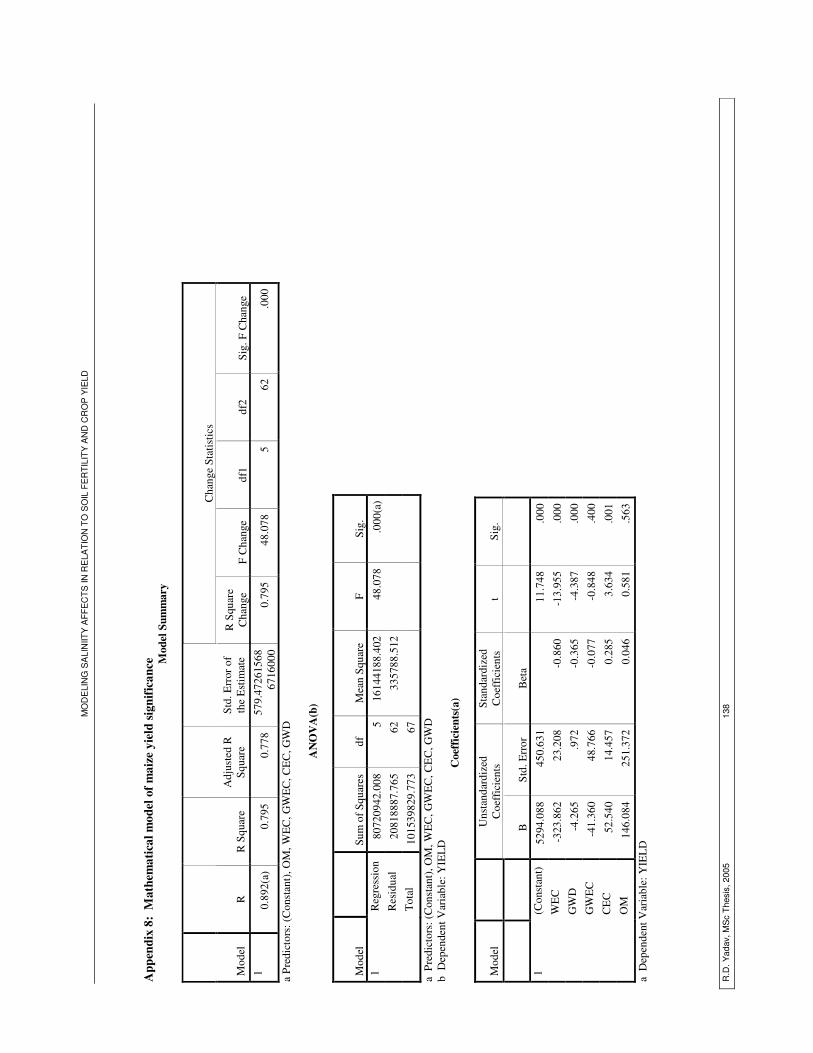
MO
DE
LIN
G S
ALI
NIIT
Y A
FFE
CT
S IN
RE
LAT
ION
TO
SO
IL F
ER
TILI
TY
AN
D C
RO
P Y
IELD
R.D
. Yad
av, M
Sc
The
sis,
200
5 13
8
App
endi
x 8:
Mat
hem
atic
al m
odel
of m
aize
yie
ld si
gnifi
canc
e
Mod
el S
umm
ary
Cha
nge
Stat
istic
s
Mod
el
R
R S
quar
e A
djus
ted
R
Squa
re
Std.
Err
or o
f th
e E
stim
ate
R S
quar
e C
hang
e F
Cha
nge
df1
df2
Sig.
F C
hang
e 1
0.89
2(a)
0.
795
0.77
8 57
9.47
2615
6867
1600
0 0.
795
48.0
78
5 62
.0
00
a Pr
edic
tors
: (C
onst
ant)
, OM
, WE
C, G
WE
C, C
EC
, GW
D
A
NO
VA
(b)
Mod
el
Su
m o
f Squ
ares
df
M
ean
Squa
re
F Si
g.
1 R
egre
ssio
n 80
7209
42.0
08
5 16
1441
88.4
02
48.0
78
.000
(a)
R
esid
ual
2081
8887
.765
62
33
5788
.512
Tota
l 10
1539
829.
773
67
a P
redi
ctor
s: (C
onst
ant)
, OM
, WE
C, G
WE
C, C
EC
, GW
D
b D
epen
dent
Var
iabl
e: Y
IELD
Coe
ffic
ient
s(a)
M
odel
Uns
tand
ardi
zed
Coe
ffic
ient
s St
anda
rdiz
ed
Coe
ffic
ient
s t
Sig.
B
Std.
Err
or
Bet
a
1
(Con
stan
t)
5294
.088
45
0.63
1
11.7
48
.000
WE
C
-323
.862
23
.208
-0
.860
-1
3.95
5 .0
00
G
WD
-4
.265
.9
72
-0.3
65
-4.3
87
.000
GW
EC
-4
1.36
0 48
.766
-0
.077
-0
.848
.4
00
C
EC
52
.540
14
.457
0.
285
3.63
4 .0
01
O
M
146.
084
251.
372
0.04
6 0.
581
.563
a D
epen
dent
Var
iabl
e: Y
IEL
D

MODELING SALINIITY AFFECTS IN RELATION TO SOIL FERTILITY AND CROP YIELD
R.D. Yadav, MSc Thesis, 2005 139
Appendix 9 (a-f) General and log transformed histogram of EC of each depth
0.000 1.000 2.000 3.000 4.000
ec0-30
0
10
20
30
40
50
60
70
Fre
qu
ency
Mean = 0.22221Std. Dev. = 0.656989N = 71
(a) EC 30
-2.00 -1.50 -1.00 -0.50 0.00 0.50
LGEC30
0
10
20
30
Fre
qu
en
cy
(d) Log EC 30
0.000 0.500 1.000 1.500 2.000
ec30-60
0
10
20
30
40
50
60
Fre
qu
en
cy
(b) EC60
(e) Log EC 60
(c) EC 90
(f) Log EC 90
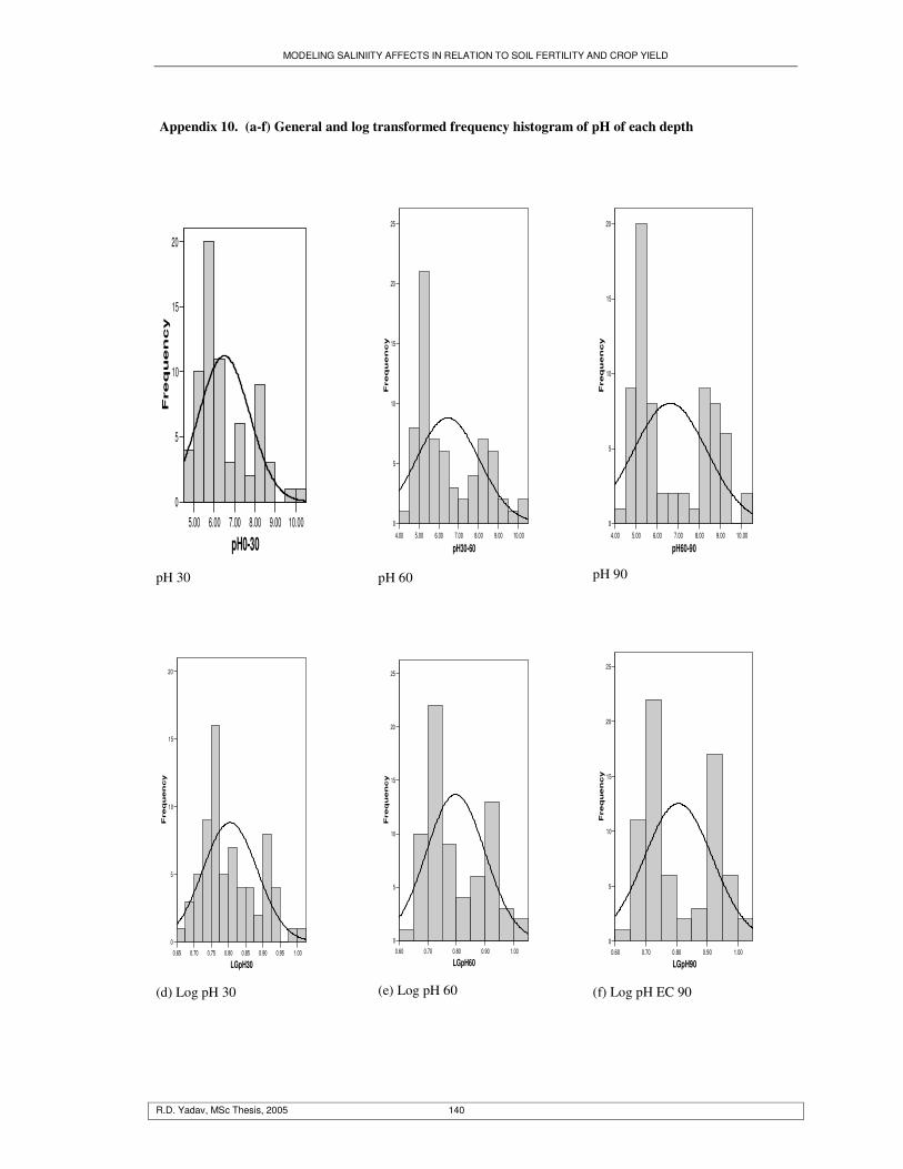
MODELING SALINIITY AFFECTS IN RELATION TO SOIL FERTILITY AND CROP YIELD
R.D. Yadav, MSc Thesis, 2005 140
Appendix 10. (a-f) General and log transformed frequency histogram of pH of each depth
5.00 6.00 7.00 8.00 9.00 10.00
pH0-30
0
5
10
15
20
Fre
qu
en
cy
pH 30
0.65 0.70 0.75 0.80 0.85 0.90 0.95 1.00
LGpH30
0
5
10
15
20
Freq
uen
cy
(d) Log pH 30
4.00 5.00 6.00 7.00 8.00 9.00 10.00
pH30-60
0
5
10
15
20
25
Freq
ue
nc
y
pH 60
0.60 0.70 0.80 0.90 1.00
LGpH60
0
5
10
15
20
25
Fre
qu
en
cy
(e) Log pH 60
4.00 5.00 6.00 7.00 8.00 9.00 10.00
pH60-90
0
5
10
15
20
Freq
ue
nc
y
pH 90
0.60 0.70 0.80 0.90 1.00
LGpH90
0
5
10
15
20
25
Fre
qu
en
cy
(f) Log pH EC 90

MODELING SALINIITY AFFECTS IN RELATION TO SOIL FERTILITY AND CROP YIELD
R.D. Yadav, MSc Thesis, 2005 141
Appendix 11. (a-d) OM and (e-h) CEC general and log transformed histogram
0.00 5.00 10.00 15.00 20.00 25.00
OM0-30
0
10
20
30
40
50
60
70
Frequ
ency
0.00 2.00 4.00 6.00 8.00 10.00 12.00
OM0-60
0
10
20
30
40
50
Freq
uenc
y
(a) (b)
-1.00 -0.50 0.00 0.50 1.00 1.50
LGOM30
0
5
10
15
20
Frequ
ency
-1.50 -1.00 -0.50 0.00 0.50 1.00
LGOM60
0
5
10
15
20
Freq
uenc
y
(c) (d)
0.00 10.00 20.00 30.00 40.00
CEC0-30
0
5
10
15
20
25
Freq
uenc
y
0.00 10.00 20.00 30.00 40.00
CEC30-60
0
5
10
15
20
25
30
Freq
uenc
y
(e) (f)
0.00 0.50 1.00 1.50
LGCEC30
0
2
4
6
8
10
12
Freq
uenc
y
(g)
0.00 0.50 1.00 1.50
LGCEC60
0
5
10
15
20
Fre
qu
ency
(h)
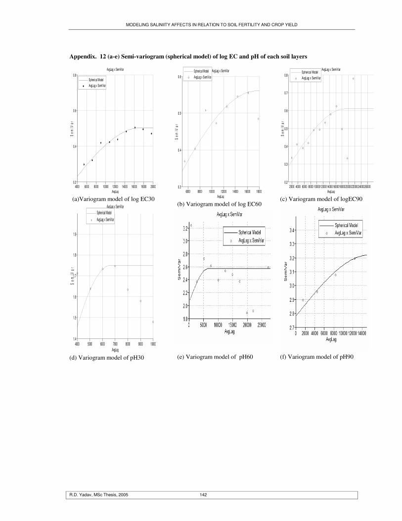
MODELING SALINIITY AFFECTS IN RELATION TO SOIL FERTILITY AND CROP YIELD
R.D. Yadav, MSc Thesis, 2005 142
Appendix. 12 (a-e) Semi-variogram (spherical model) of log EC and pH of each soil layers
AvgLag x SemiVar
4000 6000 8000 10000 12000 14000 16000 18000 20000AvgLag
0.2
0.4
0.6
0.8S
emiV
ar
Spherical ModelAvgLag x SemiVar
(a)Variogram model of log EC30
AvgLag x SemiVar
4000 5000 6000 7000 8000 9000 10000AvgLag
1.4
1.5
1.6
1.7
1.8
1.9
Sem
iVar
Spherical ModelAvgLag x SemiVar
(d) Variogram model of pH30
AvgLag x SemiVar
6000 8000 10000 12000 14000 16000 18000AvgLag
0.3
0.4
0.5
0.6
Sem
iVar
Spherical ModelAvgLag x SemiVar
(b) Variogram model of log EC60
(e) Variogram model of pH60
AvgLag x SemiVar
2000 4000 6000 8000 100001200014000160001800020000220002400026000AvgLag
0.2
0.3
0.4
0.5
0.6
0.7
0.8
Sem
iVar
Spherical ModelAvgLag x SemiVar
(c) Variogram model of logEC90
(f) Variogram model of pH90

MODELING SALINIITY AFFECTS IN RELATION TO SOIL FERTILITY AND CROP YIELD
R.D. Yadav, MSc Thesis, 2005 143
Appendix 13. Variogram model of residual logec30 and mean logec30
AvgLag x SemiVar
4000 6000 8000 10000 12000 14000 16000 18000AvgLag
0.15
0.20
0.25
0.30
0.35
Sem
iVar
Spherical ModelAvgLag x SemiVar
(a) Residual_logec30
AvgLag x SemiVar
50006000700080009000100001100012000130001400015000AvgLag
0.10
0.12
0.14
0.16
0.18
0.20
0.22
0.24
Sem
iVar
Spherical ModelAvgLag x SemiVar
(b) Mean logec30
Appendix 14. Error map of OK of each depth

MODELING SALINIITY AFFECTS IN RELATION TO SOIL FERTILITY AND CROP YIELD
R.D. Yadav, MSc Thesis, 2005 144
Appendix 15. Land suitability class and weighted map of different crops
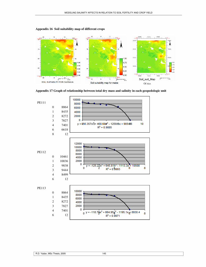
MODELING SALINIITY AFFECTS IN RELATION TO SOIL FERTILITY AND CROP YIELD
R.D. Yadav, MSc Thesis, 2005 145
Appendix 16 Soil suitability map of different crops
Appendix 17 Graph of relationship between total dry mass and salinity in each geopedologic unit
PE111
0 8864 1 8435 45 2 8272 PE114 3 7827 4 7401 6 6618 8 12
PE112
0 10461 1 10036 2 9838 3 9444 4 8499 6 12
PE113
0 8864 1 8435 2 8272 3 7827 4 7401 6 12
Of rice
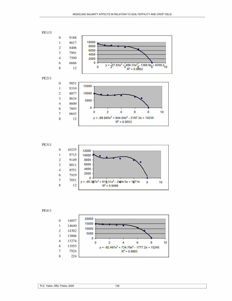
MODELING SALINIITY AFFECTS IN RELATION TO SOIL FERTILITY AND CROP YIELD
R.D. Yadav, MSc Thesis, 2005 146
PE115 0 9188 1 8617 2 8406 3 7991 4 7509 6 6666 8 12
PE211 0 9851 1 9310 2 8877 3 8624 4 8600 6 7603 7 6643 8 12
PE311
0 10235 1 9715 2 9149 3 8811 4 8551 6 7919 7 7051 8 12
PE411
0 14857
1 14640 2 14302 3 13806 4 13274 6 11055 7 7924 8 224

MODELING SALINIITY AFFECTS IN RELATION TO SOIL FERTILITY AND CROP YIELD
R.D. Yadav, MSc Thesis, 2005 147
PE412
0 13769 1 13300 2 13064 3 12493 4 11728 6 10521 7 9462 8 6185 9 12
PE413
0 15108 1 15108 2 15457 3 15447 4 15079 6 13292 8 5737 9 12
PE511
0 8419 1 8046 2 7829 3 7511 4 7211 6 6492 7 5856 8 12
PE114
0 9585 1 9149 2 8906 3 8747 4 8325 6 7088 7 6501 8 12
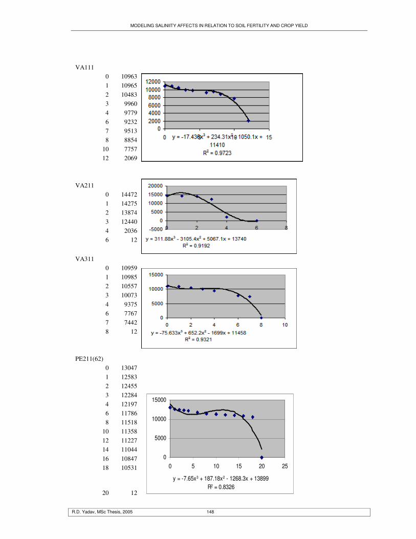
MODELING SALINIITY AFFECTS IN RELATION TO SOIL FERTILITY AND CROP YIELD
R.D. Yadav, MSc Thesis, 2005 148
VA111
0 10963 1 10965 2 10483 3 9960 4 9779 6 9232 7 9513 8 8854
10 7757 12 2069
VA211
0 14472 1 14275 2 13874 3 12440 4 2036 6 12
VA311
0 10959 1 10985 2 10557 3 10073 4 9375 6 7767 7 7442 8 12
PE211(62)
0 13047 1 12583 2 12455 3 12284 4 12197 6 11786 8 11518
10 11358 12 11227 14 11044 16 10847 18 10531
20 12
y = -7.65x3 + 187.18x2 - 1268.3x + 13899R2 = 0.8326
0
5000
10000
15000
0 5 10 15 20 25
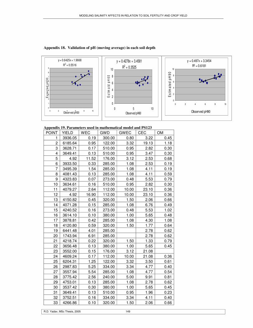
MODELING SALINIITY AFFECTS IN RELATION TO SOIL FERTILITY AND CROP YIELD
R.D. Yadav, MSc Thesis, 2005 149
Appendix 18. Validation of pH (moving average) in each soil depth
y = 0.6425x + 1.9668R2 = 0.5516
0
1
2
3
4
5
6
7
8
9
0 2 4 6 8 10Observed pH30
Exp
ecte
d pH
30
y = 0.4278x + 3.4581R2 = 0.3525
0
2
4
6
8
10
0 5 10Observed pH60
Est
imat
d pH
60
y = 0.497x + 3.3454R2 = 0.6181
0
2
4
6
8
10
0 2 4 6 8 10
Observed pH90
Est
imat
ed p
H90
Appendix 19. Parameters used in mathematical model and PS123 POINT YIELD WEC GWD GWEC CEC OM
1 3936.05 0.19 300.00 0.80 3.22 0.45 2 6185.64 0.95 122.00 3.32 19.13 1.18 3 3628.71 0.17 510.00 0.95 2.82 0.30 4 3649.41 0.13 510.00 0.95 3.47 0.30 5 4.92 11.52 176.00 3.12 2.53 0.68 6 3933.50 0.33 285.00 1.08 2.53 0.19 7 3495.39 1.54 285.00 1.08 4.11 0.19 8 4081.43 0.13 285.00 1.08 4.11 0.59 9 4323.83 0.07 273.00 0.48 5.53 0.79
10 3634.61 0.16 510.00 0.95 2.82 0.30 11 4079.27 2.64 112.00 10.00 23.10 0.36 12 4.92 16.90 112.00 10.00 23.10 0.36 13 4150.82 0.45 320.00 1.50 2.06 0.66 14 4071.28 0.15 285.00 1.08 6.76 0.49 15 4240.52 0.16 273.00 0.48 5.53 1.02 16 3614.10 0.10 380.00 1.00 5.65 0.48 17 3878.81 0.42 285.00 1.08 4.30 1.08 18 4120.80 0.59 320.00 1.50 1.77 0.64 19 6441.48 4.01 285.00 2.78 0.62 20 1743.94 6.91 285.00 2.78 0.62 21 4218.74 0.22 320.00 1.50 1.33 0.79 22 3656.48 0.13 380.00 1.00 5.65 0.45 23 3552.00 0.15 176.00 3.12 21.08 24 4609.24 0.17 112.00 10.00 21.08 0.36 25 6204.31 1.25 122.00 3.32 3.50 0.61 26 2987.83 5.25 334.00 3.34 4.77 0.40 27 3557.94 5.54 285.00 1.08 4.77 0.54 28 3775.42 2.56 240.00 5.00 9.91 0.81 29 4753.01 0.13 285.00 1.08 2.78 0.62 30 3537.42 0.30 380.00 1.00 5.65 0.45 31 3649.41 0.13 510.00 0.95 1.96 0.23 32 3752.51 0.16 334.00 3.34 4.11 0.40 33 4266.86 0.10 320.00 1.50 2.06 0.66
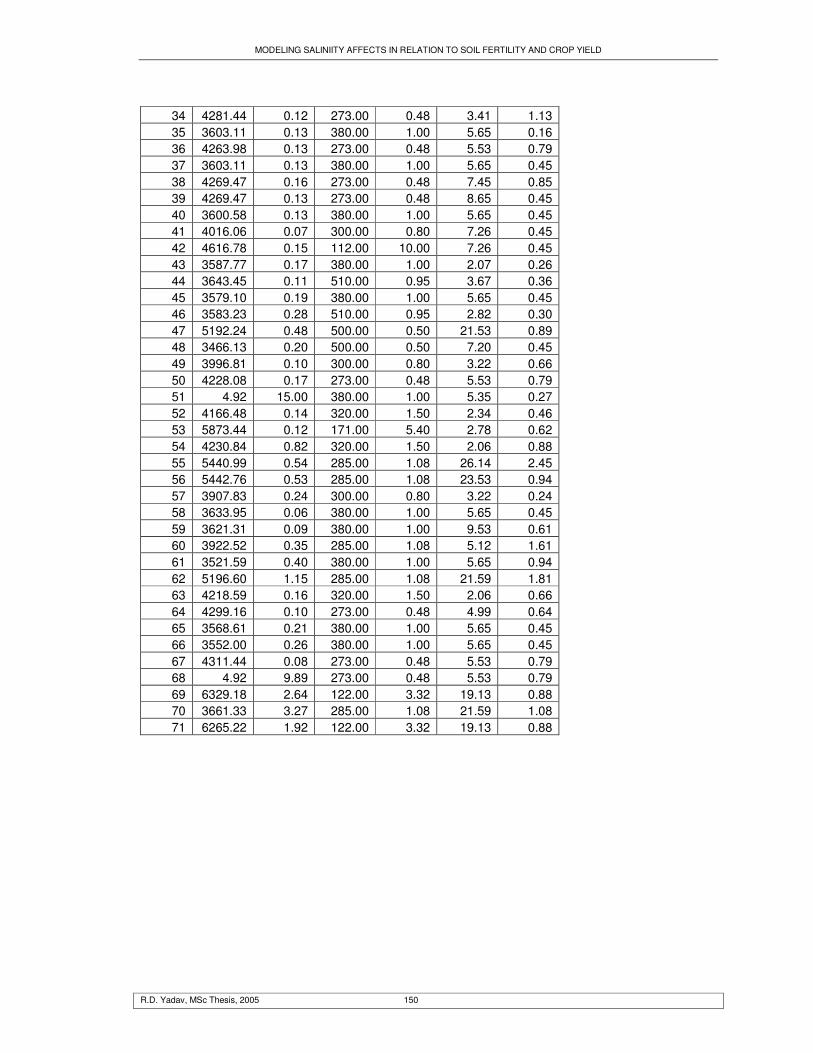
MODELING SALINIITY AFFECTS IN RELATION TO SOIL FERTILITY AND CROP YIELD
R.D. Yadav, MSc Thesis, 2005 150
34 4281.44 0.12 273.00 0.48 3.41 1.13 35 3603.11 0.13 380.00 1.00 5.65 0.16 36 4263.98 0.13 273.00 0.48 5.53 0.79 37 3603.11 0.13 380.00 1.00 5.65 0.45 38 4269.47 0.16 273.00 0.48 7.45 0.85 39 4269.47 0.13 273.00 0.48 8.65 0.45 40 3600.58 0.13 380.00 1.00 5.65 0.45 41 4016.06 0.07 300.00 0.80 7.26 0.45 42 4616.78 0.15 112.00 10.00 7.26 0.45 43 3587.77 0.17 380.00 1.00 2.07 0.26 44 3643.45 0.11 510.00 0.95 3.67 0.36 45 3579.10 0.19 380.00 1.00 5.65 0.45 46 3583.23 0.28 510.00 0.95 2.82 0.30 47 5192.24 0.48 500.00 0.50 21.53 0.89 48 3466.13 0.20 500.00 0.50 7.20 0.45 49 3996.81 0.10 300.00 0.80 3.22 0.66 50 4228.08 0.17 273.00 0.48 5.53 0.79 51 4.92 15.00 380.00 1.00 5.35 0.27 52 4166.48 0.14 320.00 1.50 2.34 0.46 53 5873.44 0.12 171.00 5.40 2.78 0.62 54 4230.84 0.82 320.00 1.50 2.06 0.88 55 5440.99 0.54 285.00 1.08 26.14 2.45 56 5442.76 0.53 285.00 1.08 23.53 0.94 57 3907.83 0.24 300.00 0.80 3.22 0.24 58 3633.95 0.06 380.00 1.00 5.65 0.45 59 3621.31 0.09 380.00 1.00 9.53 0.61 60 3922.52 0.35 285.00 1.08 5.12 1.61 61 3521.59 0.40 380.00 1.00 5.65 0.94 62 5196.60 1.15 285.00 1.08 21.59 1.81 63 4218.59 0.16 320.00 1.50 2.06 0.66 64 4299.16 0.10 273.00 0.48 4.99 0.64 65 3568.61 0.21 380.00 1.00 5.65 0.45 66 3552.00 0.26 380.00 1.00 5.65 0.45 67 4311.44 0.08 273.00 0.48 5.53 0.79 68 4.92 9.89 273.00 0.48 5.53 0.79 69 6329.18 2.64 122.00 3.32 19.13 0.88 70 3661.33 3.27 285.00 1.08 21.59 1.08 71 6265.22 1.92 122.00 3.32 19.13 0.88