modeling photon generation - information services ...rmoore/mpi2011/mckinstriempi11talks.pdf ·...
TRANSCRIPT

•
June 2011Mathematical Problems in Industry
Modeling photon generation
C. J. McKinstrie
Bell Laboratories, Alcatel-Lucent
•
2MPI, June 2011
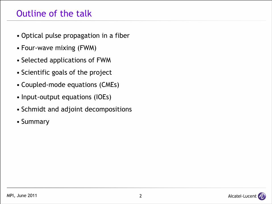
Outline of the talk
•
Optical pulse propagation in a fiber
•
Four-wave mixing (FWM)
•
Selected applications of FWM
•
Scientific goals of the project
•
Coupled-mode equations (CMEs)
•
Input-output equations (IOEs)
•
Schmidt and adjoint
decompositions
•
Summary
•
3MPI, June 2011
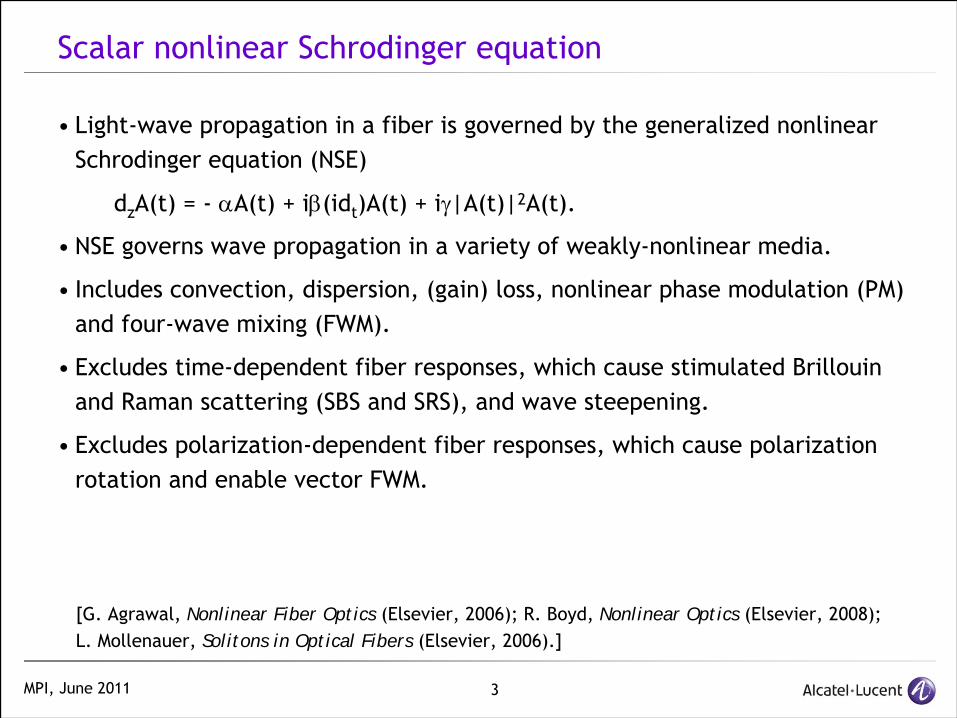
Scalar nonlinear Schrodinger equation
•
Light-wave propagation in a fiber is governed by the generalized nonlinear Schrodinger equation (NSE)
dz
A(t) = -
αA(t) + iβ(idt
)A(t) + iγ|A(t)|2A(t).
•
NSE governs wave propagation in a variety of weakly-nonlinear media.
•
Includes convection, dispersion, (gain) loss, nonlinear phase modulation (PM) and four-wave mixing (FWM).
•
Excludes time-dependent fiber responses, which cause stimulated Brillouin
and Raman scattering (SBS and SRS), and wave steepening.
•
Excludes polarization-dependent fiber responses, which cause polarization rotation and enable vector FWM.
[G. Agrawal, Nonlinear Fiber Optics (Elsevier, 2006); R. Boyd, Nonlinear Optics (Elsevier, 2008); L. Mollenauer, Solitons in Optical Fibers (Elsevier, 2006).]
•
4MPI, June 2011
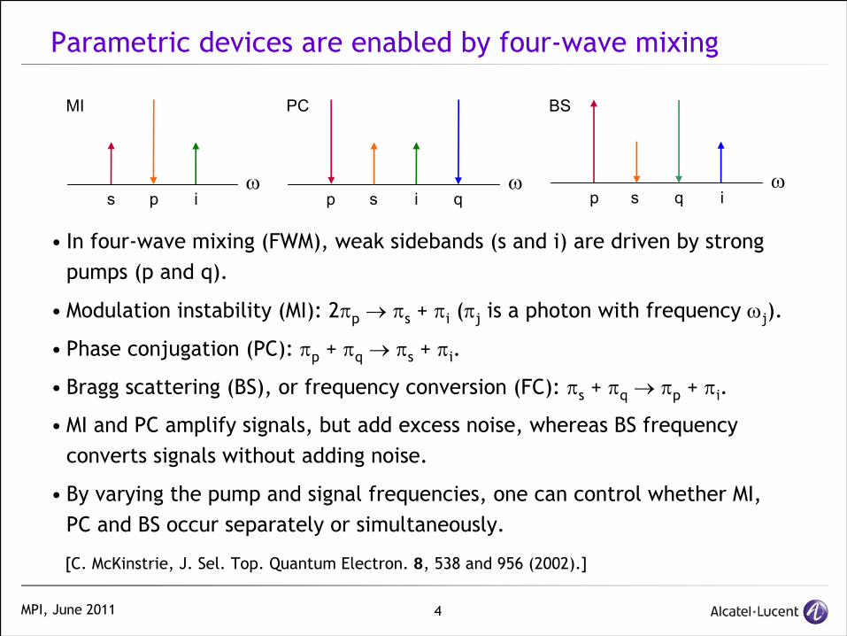
Parametric devices are enabled by four-wave mixing
•
In four-wave mixing (FWM), weak sidebands (s and i) are driven by strong
pumps (p and q).
•
Modulation instability (MI): 2πp
→ πs
+ πi
(πj
is a photon with frequency ωj
).
•
Phase conjugation (PC): πp
+ πq
→ πs
+ πi
.
•
Bragg scattering (BS), or frequency conversion (FC): πs
+ πq
→ πp
+ πi
.
•
MI and PC amplify signals, but add excess noise, whereas BS frequency converts signals without adding noise.
•
By varying the pump and signal frequencies, one can control whether MI, PC and BS occur separately or simultaneously.
[C. McKinstrie, J. Sel. Top. Quantum Electron. 8, 538 and 956 (2002).]
ωs q ip
BS
ωs i qp
PC
s p iω
MI

•
5MPI, June 2011
Degenerate four-wave mixing
•
In degenerate FWM, also called modulation interaction (MI), a strong pump (p) drives a weak signal and idler (s, i). The frequency-matching (FM) condition is 2ωp
=
ωs
+ ωi
.
dz
As
= i(βs
+ 2γ|Ap
|2)As
+ iγAp2Ai
*,
dz
Ap
≈
i(βp
+ γ|Ap
|2)Ap
,
dz
Ai
= i(βi
+ 2γ|Ap
|2)As
+ iγAp2As
*.
•
Remove pump phase factor: Aj
(z) = Bj
(z)exp[i(βp
+ γP)z], where P = |Ap
|2.
dz
Bs
= i(βs
-
βp
+ γP)Bs
+ iγBp2Bi
*,
dz
Bi
= i(βi
-
βp
+ γP)Bi
+ iγBp2Bs
*.
•
Conjugate the i-equation and look for eigenvalues
(MI wavenumbers) k.
k = (δs
–
δi
)/2 ±
[(δs
+ δi
)2/4 -
(γP)2]1/2, where δj
= βj
-
βp
+ γP.
•
Define the (wavenumber) mismatch δ
= (δs
+ δi
)/2 = (βs
– 2βp
+ βi
)/2 + γP.
•
If |δ| > γP, then k is real; the MI is stable, (s and i) sidebands do not grow.
•
If |δ| < γP, then k is imaginary; the MI is unstable, sidebands grow.
[C. McKinstrie, J. Sel. Top. Quantum Electron. 8, 538 & 956 (2002).]

•
6MPI, June 2011
When is the MI unstable?
•
Expand the wavenumbers
about the pump frequency.
βj
(ωj
) = β0
(ωp
) + β1
(ωp
)(ωj
–
ωp
) + β2
(ωp
)(ωj
–
ωp
)2/2; ωs,i
= ωp
± ω,
2δ
= [β0
(ωp
) + β1
(ωp
)ω
+ β2
(ωp
)ω2/2] -
2β0
(ωp
)
+
[β0
(ωp
) -
β1
(ωp
)ω
+ β2
(ωp
)ω2/2] + 2γP = β2
(ωp
)ω2
+ 2γP.
•
If β2
(ωp
) > 0 (normal dispersion), then |δ| > γP; MI is stable.
•
If -4γP < β2
(ωp
)ω2
< 0 (anomalous dispersion), then |δ| > γP; MI is unstable.
•
The maximal spatial growth rate γP
is attained when ω
= (2γP/|β2
|)1/2.
•
In the presence of higher-order dispersion, extra gain bands can exist.
-75
-55
-35
-15
5
1560 1570 1580 1590 1600
λ0(dB)
(nm)

•
7MPI, June 2011
Input-output equations for MI
•
Let Bs
= Cs
exp[i(δs
-
δi
)z/2] and Bi
= Ci
exp[i(δi
–
δs
)z/2]. Then the MI equations can be written in the symmetric form
dz
Cs
= iδCs
+ iγBp2Ci
*, dz
Ci
* = -iδCi
* -
iγ(Bp
*)2Cs
,
where the (common) mismatch δ
= (δs
+ δi
)/2.
•
The solutions of the MI equations can be written in the input-output form
Cs
(z) = μ(z)Cs
(0) + ν(z)Ci
(0), Ci
*(z) = ν*(z)Cs
(0) + μ*(z)Ci
*(0),
where the transfer (Green) functions
μ(z) = cos(kz) + iδsin(kz)/k, ν(z) = iγBp2sin(kz)/k
and the MI wavenumber
k = [δ2
- (γP)2]1/2.
•
Notice that |μ(z)|2
- |ν(z)|2
= 1, from which it follows that
|Cs
(z)|2
- |Ci
(z)|2
= [|μ(z)|2
- |ν(z)|2][|Cs
(0)|2
- |Ci
(0)|2] = |Cs
(0)|2
- |Ci
(0)|2.
•
Sideband photons are created in pairs (linear theory)!
[C. McKinstrie, Opt. Express 12, 5037 (2004).]
•
8MPI, June 2011
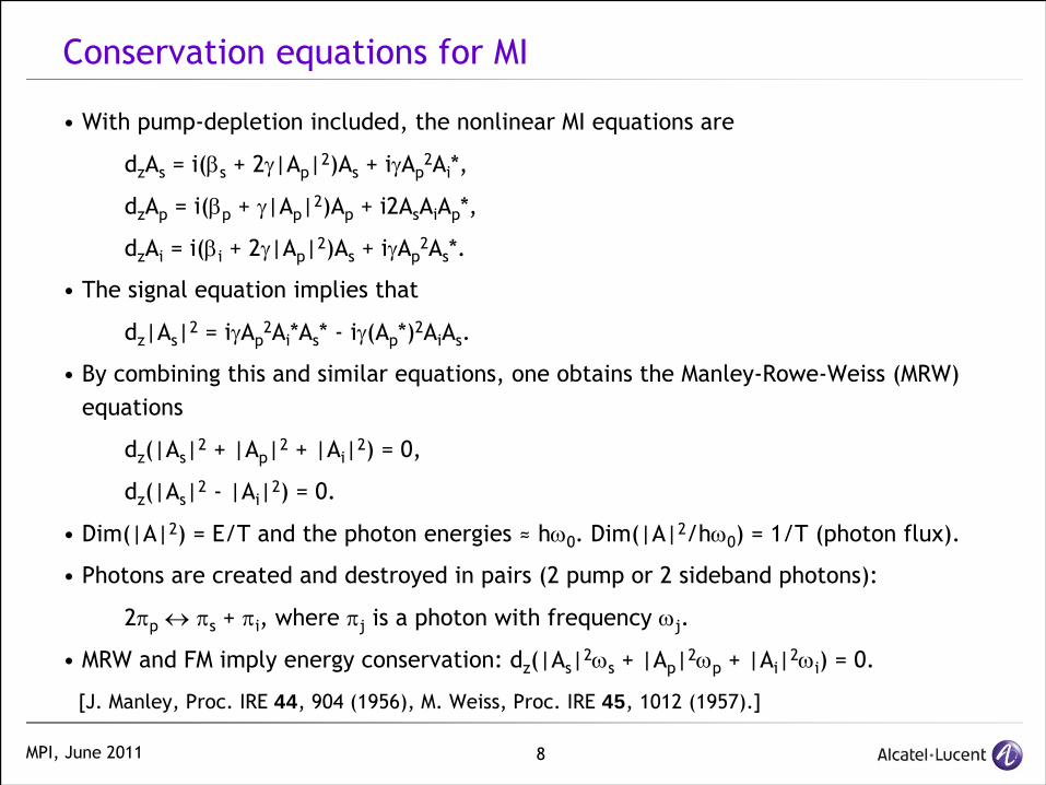
Conservation equations for MI
•
With pump-depletion included, the nonlinear MI equations are
dz
As
= i(βs
+ 2γ|Ap
|2)As
+ iγAp2Ai
*,
dz
Ap
= i(βp
+ γ|Ap
|2)Ap
+ i2As
Ai
Ap
*,
dz
Ai
= i(βi
+ 2γ|Ap
|2)As
+ iγAp2As
*.
•
The signal equation implies that
dz
|As
|2
= iγAp2Ai
*As
* -
iγ(Ap
*)2Ai
As
.
•
By combining this and similar equations, one obtains the Manley-Rowe-Weiss (MRW) equations
dz
(|As
|2
+ |Ap
|2
+ |Ai
|2) = 0,
dz
(|As
|2
- |Ai
|2) = 0.
•
Dim(|A|2) = E/T and the photon energies ≈
hω0
. Dim(|A|2/hω0
) = 1/T (photon flux).
•
Photons are created and destroyed in pairs (2 pump or 2 sideband
photons):
2πp
↔ πs
+ πi
, where πj
is a photon with frequency ωj
.
•
MRW and FM imply energy conservation: dz
(|As
|2ωs
+ |Ap
|2ωp
+ |Ai
|2ωi
) = 0.
[J. Manley, Proc. IRE 44, 904 (1956), M. Weiss, Proc. IRE 45, 1012 (1957).]

•
9MPI, June 2011
Radiation generation in photonic-crystal fiber
•
Singly-resonant OPO: PCF (l = 1.3 m, γ
= 110/Km-W), pulsed pump (τ
= 8 ps, λ
≈
710 nm, P > 15 W), dichroic
mirrors. Frequency shifts from 20 –
170 THz.•
Performance was limited by pump-sideband walk-off.
[Y. Xu, Opt. Lett. 33, 1351 (2008); S. Murdoch (2009).]
(S: 770–1150 nm)
(aS: 510-690 nm)

•
10MPI, June 2011
Broad-bandwidth amplification for communication
•
Parametric amplifiers have broader gain bandwidths than their competitors.
•
The current record bandwidth is 150 nm (signal plus idler).
•
Perpendicular pumps provide signal-polarization-independent gain.
•
Standard system with 128 channels at 10 Gb/s
requires 51 nm bandwidth.
•
Latest system (AL 1830) with 88 channels at 100 Gb/s
requires 35 nm.
15
20
25
30
35
1560 1580 1600
Parametric AmpRaman Amp, one pumpErbium Fiber Amp (shifted 30 nm)
Wavelength (nm)
Gai
n (d
B)
[R. Jopson
(2004); J. Chavez Boggio, Photon. Technol. Lett. 21, 612 (2009).]
•
11MPI, June 2011
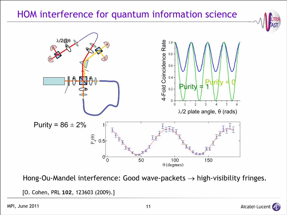
HOM interference for quantum information science
λ/2 plate angle, θ
(rads)
4-Fo
ld C
oinc
iden
ce R
ate
Purity = 1Purity = 0
λ/2@θ
D
BA
C
λ/2@θ
D
BA
C
Purity = 86 ±
2%
[O. Cohen, PRL 102, 123603 (2009).]
•Hong-Ou-Mandel interference: Good wave-packets →
high-visibility fringes.

•
12MPI, June 2011
General scientific goals
•
High-gain FWM amplifies input signals and generates idlers, or generates signals and idlers from noise.
•
Low-gain FWM generates photon pairs (1 signal and 1 idler photon).
•
FWM also frequency converts input signals without gain.
•
Tutorial discussion pertained to monochromatic, or continuous-wave (CW), pump, signal and idler waves. In many applications, the waves are pulses.
•
What are the generated photon pulses (wave-packets) like and how do they depend on the system (fiber and pump) parameters? How do we tailor them for applications in quantum information science?
•
What input pulses optimize the operations of FWM processes (amplification, frequency conversion, pulse reshaping)?
•
13MPI, June 2011
Coupled-mode equations
•
Signal and idler evolution is governed by the coupled-mode equation (CME)
dX/dz
= iAX
+ iBX*,
where A is hermitian
and B is symmetric (QM).
•
S and I each have 1 F-component: X = [As
,Ai
]t.
•
S and I have 1 F-
and 2 P-components: X = [Asx
,Asy
,Aix
,Aiy
]t.
•
S and I have n F-components: X is a 2n x 1 vector.
•
S and I have n F-
and 2 P-components: X is a 4n x 1 vector.
•
Question: Under what conditions can the CME be solved analytically?
•
If A and B are simultaneously diagonalizable, then dxj
/dz
= iαj
xj
+ iβj
xj+,
where xj
is an e-amplitude, and αj
and βj
are e-values (1-mode squeezing).
•
In most applications, A and B are not simultaneously diagonalizable!
•
14MPI, June 2011
Singular value (Schmidt) decomposition
•
Every complex matrix M = UDV+, where U and V are unitary and D is diagonal.
•
The columns of U are e-vectors of MM+
and the columns of V are e-vectors of M+M. These e-vectors are called Schmidt modes.
•
The entries of D (Schmidt coefficients σ) are the square roots of the (common) non-negative e-values of MM+
and M+M.
•
M = UDV+
is equivalent to M = Σj
Uj
σj
Vj+.
•
Consider Y = MX, where X and Y are input and output vectors: M resolves input modes ―
dilates mode amplitudes ―
projects output modes.
•
SVD common in numerical mathematics (e.g. least squares minimization, linear equations). Recently became common in theoretical quantum
optics.
[G. Stewart, SIAM Rev. 35, 551 (1993).]

•
15MPI, June 2011
Input-output equations
•
Consider the IOE X(z) = M(z)X(0) + N(z)X*(0); M and N are transfer matrices.
•
Abbreviate as Y = MX + NX*; X and Y are input and output vectors.
•
Individual SVDs
M = Uμ
Dμ
Vμ+
and N = Uν
Dν
Vν+
are not useful by themselves.
•
QM requires that MM+
- NN+
= I, i.e. Uμ
Dμ2Uμ
+
- Uν
Dν2Uν
+
= I. Hence, Um
= Uν
and μj
2
–
νj2
= 1.
•
The inverse transformation is X = M+Y –
NtY*. QM requires that M+M –
NtN* = I, i.e. Vμ
Dμ2Vμ
+
- Vν
*Dν2Vν
t
= I. Hence, Vμ
= Vν
*.
•
M and N have simultaneous SVDs: Y = UDμ
V+X + UDν
VtX*.
•
Define yj
= Uj+Y and xj
= Vj+X. Then yj
= μj
xj
+ νj
xj+.
•
Each input-mode operator is related to a single output-mode operator by a 1-mode squeezing transformation (simple)!
•
Comments: The Schmidt coefficients and modes depend on z.
The theorem does not tell us how to determine M and N.
[S. Braunstein, Phys. Rev. A 71, 055801 (1995); C. McKinstrie, Opt. Commun. 282, 583 (2009).]
•
16MPI, June 2011
The adjoint
method works well
•
dX/dz
= iAX
+ iBX* and its conjugate can be rewritten as dY/dz
= iLY, where Y = [X,X*]t
and L = [A, B; B*, A*] is not self-adjoint.
•
Determine the e-vectors (LEj
= λj
Ej
) and adjoint
e-vectors (L+Fj
= λj
*Fj
).
•
The e-vectors are bi-orthogonal: Fj+Ek
= δjk
or F+E = I.
•
Adjoint
decomposition: L = Σj
Ej
λj
Fj+
= EDλ
F+.
•
exp(iLz) = Σj
Ej
exp(iλj
z)Fj+
and exp(iLz2
)exp(iLz1
) = exp[iL(z1
+z2
)].
•
Comment: The e-vectors Ej
and Fj
do not depend on z and the propagation coefficients exp(iλj
z) depend simply on z. Transfer matrices concatenate.
•
Question: What is the physical significance of the e-modes, which involve xj
and xj+, so are not superposition modes?
[C. McKinstrie, Opt. Commun. 282, 583 (2009).]

•
17MPI, June 2011
Follow the breadcrumbs!
•
Consider the CME dY/dz
= iLY. L is almost hermitian:
L = [A, B; -B*, -A*] = S1
H where S1
= [I,0; 0, -I] and H = [A, B; B*, A*]. Properties of e-values and e-vectors?
•
Consider the IOE Y(z) = T(z)Y(0): T = [M, N; N*, M*] is symplectic:
TS2
Tt
= S2
, where S2
= [0, I; -I, 0]. (MM+
- NN+
= I, MNt
– NMt
= 0.)
•
The CME and IOE can be reformulated in terms of real quantities:
L →
real non-symmetric and T →
real symplectic?
[R. Littlejohn, Rep. Phys. 138, 193 (1986); R. Gilmore, Lie Groups (Dover, 2006); C. McKinstrie, J. Sel. Top. Quantum Electron. (2011).]
•
18MPI, June 2011
Summary
•
CMEs
govern a variety of parametric processes in classical communications and quantum information science.
•
It is important to determine the natural input and output modes of these processes, and how they depend on the system parameters.
•
The mathematics of CMEs
(IOEs) involve Schmidt and adjoint
decompositions.
•
The relation between these decompositions requires further study!