TRANSPORT PROBLEMS 2017 Volume 12 Issue 3 PROBLEMY TRANSPORTU DOI: 10.20858/tp.2017.12.3.1

Keywords: electric traction; power supply; controlling; modeling, space-time; voltage stabilization

Dmitry BOSYI*, Yevhen KOSARIEV Dnipropetrovsk National University of Railway Transport Lazaryana 2, 49010, Dnipro, Ukraine *Corresponding author. E-mail: dake@i.ua MODELING OF THE CONTROLLED TRACTION POWER SUPPLY SYSTEM IN THE SPACE-TIME COORDINATES

Summary. The problems of the traction power supply system calculation are considered in the article. The authors proposed the space-time model, which is based on the analytical functions of the current- and voltage-drop distributions in the contact network. The usage of the proposed model is shown for the control law calculation both to stabilize the voltage at the pantographs of the electric rolling stocks and to reduce the power losses.

1. INTRODUCTION

The traction power supply system is a very difficult system, requiring various factors to be considered for its calculation. The methods and the means depend on the chosen factors that also have an effect on the volumes of data and the performance of the simulation process [1]. As usual the models of the traction power supply systems are used for electrical characteristics used in designing or for the mode optimization during operation. Also, these models are useful for the implementation of new devices and when the abnormal modes occur.

The calculations of the controlled traction power supply systems are more difficult. This means that additional elements must be included into evaluation with a variable parameter. First of all the control systems or its separate components may be considered as these elements. Also, volumes of the processing data are increasing for when the system reaction needs to be defined based on the internal or external influences or their combination [2, 3].

Such widely known specialized software programs as Nord, Fazonord, Flow3, and KORTES are used for traction power system simulation. These program packages were developed by Railway Research Institute (VNIIZhT) and Irkutsk State University of Railway Transport (IrSURT) [4]. DNURT has similar projects, known as PrEns and Matrix. These programs allow to simulate a locomotive’s movement control and its interaction with the traction power supply system. Other scientists [5-8] used the universal modeling system such as OrCAD, TCAD, MatLAB, and LabView for single modes of the traction and external power supply system simulation. These systems have a powerful library of electronic and power electronic devices but the one that is traction supply-specific is difficult to take into account. For example, such known work as [7-9] research the traction power supply system as a discrete system in the time dimension, which is insufficient in the point of view of continuous movement.

The results of the traction power supply evaluation in the space–time coordinates are the most generalizing, and optimization calculations could not be made without it, because the traction load changes its characteristics at the same time in two dimensions [12].

Thus, the aim of this work is to show how to use the space–time method to calculate the traction power supply system with an outlook of intelligent system control.

6 D. Bosiy, Ye. Kosariev 2. BASE PRINCIPLES OF THE METHODIC

The space–time model of the traction power supply system is based on the analytical description of the

main electrical process with a function of two variables. The train-table ( ),ttx n t defines the interconnection

between two coordinates of time t and distance x . Physically, ( ),ttx n t represents the scheduled dislocation of the train with number n in any moment of time t . Using the other input data, which define the current profile of the loads ( ),eI n t , the parameters of the traction network{ }0,S r and the external power

supply system are as follows: primary voltage prU , short-circuit power ftS , nominal power nS , and

coefficient of the rectifier A compose the space–time model of the traction power supply system (fig. 1). The output results of the model are the functions which define the voltages on the train’s pantographs ( ),eU n t

and the power losses in the contact line network ( ),CP t x∆ .

Fig. 1. The structure of the space–-time model of the traction power supply system

The results of the models were received through the definitions of feeder currents ( ),FI n t (2-7),

current distribution in the contact network ( ),CI t x (16), and the distribution of the voltage drops

( ),CU t x∆ (21), which will be described further.

Modeling of the controlled traction power supply system in the space-time coordinates 7 .

Feeder currents ( ),FI n t are defined as current profile multiplied by a current distribution function from one traction load. Next, we obtain current distribution in a contact line of one train. After we summarize this current due to distance–time curve, we get a distribution of current from all trains on the track. Because of the the primary system parameters and feeder current, we can obtain a DC voltage dU

on the traction substation bus. Using the voltage dU , scheme parameters { }0,S r , and current distribution of one train we can get a voltage-drop distribution along each track. The voltage-drop distribution from all trains is obtained by summarizing each train’s voltage drop.

For simplifying the following graphics the constant profile of the traction load, the fixed parameters of the external and traction power network, and the example of the train-table (fig. 2) will be used. In fig. 2. the numbers indicate the serial number of the train. However, in a real condition, voltage-dependent parameters may also be taken into account.

Fig. 2. The train-table example for calculations 2.1. Feeder current calculation

The functions of current distribution method is used for the quick calculation of instantaneous

schemes. The function of current distribution ( )xϕ is the part of the traction current ( )еI x in every point with an x coordinate, which shows a part of the load current that is consumed by a certain feeder of traction substation

( )( )( )

Fii

е

I xxI x

ϕ = , (1)

where i is the number of the traction substation feeder (for double-track i = 4).

From the formula (1) the value of feeder current ( )FiI x may be calculated as the traction current ( )еI x multiplied by the function ( )i xϕ that is defined for every scheme of traction network

assuming that voltages of traction substations are equal and constant. The feeder current of the separate catenary systems for double track railway (fig. 3) in analytical

expression may be expressed as follows

( )1 ( )F eL xI x I x

L−

= ; (2)

( )2 ( )F exI x I xL

= . (3)

where L is the distance between a pair of traction substations, expressed in kms.

8 D. Bosiy, Ye. Kosariev

In the case of the single-node power scheme (fig. 4) the analytical expression of the currents of feeders are more complex.

( )1

1 , 0 ;2

( )1 1 , ;2

spsp

spF e

sp

L lx x l

LlI x I x

x l x LL

+− ≤ ≤

= ⋅ − ≤ ≤

(4)

( )2

, 0 ;2

( )1 1 , ;2

spsp

spF e

sp

L lx x l

LlI x I x

x l x LL

−≤ ≤

= ⋅ − ≤ ≤

(5)

( ) ( )( )( )

3

, 0 ;2

( ) 21 , ;

2

sp

F e spsp

sp

x x lL

I x I x L l L xl x L

L L l

≤ ≤= ⋅ − − − ≤ ≤ −

(6)

( ) ( )( )

4

, 0 ;2

( ), ;

2

sp

F e spsp

sp

x x lL

I x I x l L xl x L

L L l

≤ ≤= ⋅ − ≤ ≤ −

(7)

where spl is the location of the sectioning post counting from the first substation, expressed in kms.

Fig. 3. The separate catenary systems for double-track railway (top) and its functions of current distribution (bottom) when the train is located on the first track (a) or the second track (b)

Modeling of the controlled traction power supply system in the space-time coordinates 9 .

Fig. 4. The single-node power scheme of traction network (top) and its functions of current distribution (bottom) when a train is located on the first track (a) or the second track (b)

The expression of the feeder current for a scheme with three parallel connections of the catenary

between a pair of traction substations (fig. 5) assuming that the resistance of a tie post is equal to zero will be as follows:

( )

11

11

1

1 , 0 ;2

( )1 1 , ;2

tptp

tpF e

tp

L lx x l

LlI x I x

x l x LL

+− ≤ ≤

= ⋅ − ≤ ≤

(8)

( )

11

12

1

, 0 ;2

( )1 1 , ;2

tptp

tpF e

tp

L lx x l

LlI x I x

x l x LL

−≤ ≤

= ⋅ − ≤ ≤

(9)

( ) ( )( )( )

2

3 22

2

, 0 ;2

( ) 21 , ;

2

tp

F e tptp

tp

x x lL

I x I x L l L xl x L

L L l

≤ ≤= ⋅ − − − ≤ ≤ −

(10)

( ) ( )( )

2

4 22

2

, 0 ;2

( ), ;

2

tp

F e tptp

tp

x x lL

I x I x l L xl x L

L L l

≤ ≤= ⋅ − ≤ ≤ −

(11)

where 1tpl , 2tpl are the locations of the point of parallelizing the pair of catenary systems (tie posts) along the track, expressed in kms.

10 D. Bosiy, Ye. Kosariev

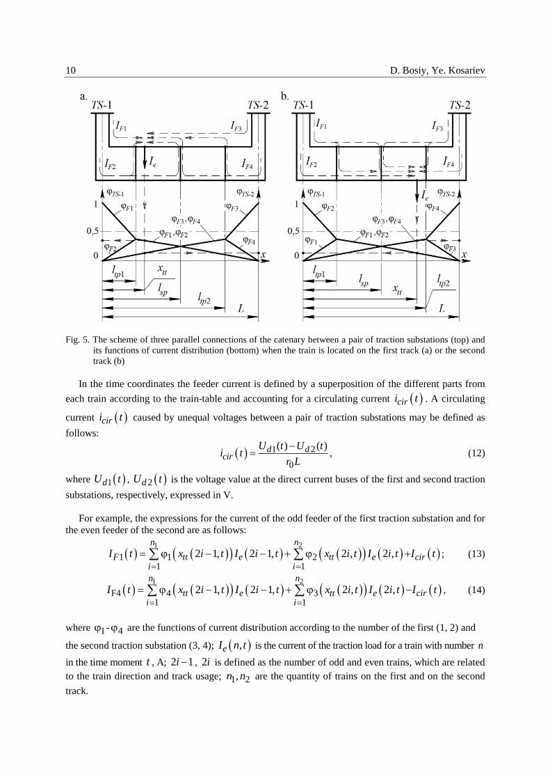
Fig. 5. The scheme of three parallel connections of the catenary between a pair of traction substations (top) and its functions of current distribution (bottom) when the train is located on the first track (a) or the second track (b)

In the time coordinates the feeder current is defined by a superposition of the different parts from

each train according to the train-table and accounting for a circulating current ( )ciri t . A circulating

current ( )ciri t caused by unequal voltages between a pair of traction substations may be defined as follows:

( ) 1 2

0

( ) ( )d dcir

U t U ti tr L−

= , (12)

where ( )1dU t , ( )2dU t is the voltage value at the direct current buses of the first and second traction substations, respectively, expressed in V.

For example, the expressions for the current of the odd feeder of the first traction substation and for the even feeder of the second are as follows:

( ) ( )( ) ( ) ( )( ) ( ) ( )1 2

1 1 21 1

2 1, 2 1, 2 , 2 ,n n

F tt e tt e ciri i

I t x i t I i t x i t I i t I t= =

= ϕ − − + ϕ +∑ ∑ ; (13)

( ) ( )( ) ( ) ( )( ) ( ) ( )1 2

F4 4 31 1

2 1, 2 1, 2 , 2 ,n n

tt e tt e ciri i

I t x i t I i t x i t I i t I t= =

= ϕ − − + ϕ −∑ ∑ , (14)

where 1ϕ - 4ϕ are the functions of current distribution according to the number of the first (1, 2) and

the second traction substation (3, 4); ( ),eI n t is the current of the traction load for a train with number n in the time moment t , A; 2 1i − , 2i is defined as the number of odd and even trains, which are related to the train direction and track usage; 1 2,n n are the quantity of trains on the first and on the second track.

Modeling of the controlled traction power supply system in the space-time coordinates 11 . 2.2. Calculation of the currents distribution in the contact network

The current distribution in the contact line may be expressed using given feeder currents from one

train in the train-table. For the first, the distribution of currents in a power scheme must be defined from one load. In general, for the single-node power scheme and the first or second track (fig. 6, 7), this expression was obtained by analyzing the current distribution in the contact line, and expression takes the form (15).

Fig. 6. The single-node power scheme of a traction network (top) and its current distribution in a contact line on the first track (bottom) when the train is located on the first track before the sectioning post (a) and behind the sectioning post (b)

Fig. 7. The single-node power scheme of traction network (top) and its current distribution in contact line on the first track (bottom) when train is located on second track before the sectioning post (a) and behind the sectioning post (b)

12 D. Bosiy, Ye. Kosariev

( )

( ) ( )( ) ( )

( )

( )

( )( ) ( )

( ) ( )

( )

( )

F1

F C C2,3,4

F3 C

1 F1 C

F C C1,2,4

F3

F1

, , 0 , ;

, , , ; ,0 , ;

, , ;, 2 1;

, , , , 0 ;

, , , ; , , ;

, , , ;

, ,

tt

i tt tti

C

i tt tti

tt

I n t x x n t

I n t x n t x l x n t l

I n t l x Ln i

i n t x I n t x l

I n t l x x n t l x n t L

I n t x n t x L

I n t

=

=

≤ ≤− < ≤ ≤ ≤

− < ≤ = −

= ≤ ≤ < ≤ < ≤ − < ≤

∑

∑

( )C

F3 C

0 ;, 2 .

, , ;

x ln i

I n t l x L

≤ ≤ = − < ≤

(15)

where ( ),FiI n t are the currents of each feeder (i=1..4) from the train with number n in the moment of time t .

With the help of superposition the current distribution in the contact network is defined for all trains in the train-table while accounting for a circulating current ( )ciri t .

For example, the expression for the contact network of the first track will be as follows

( ) ( ) ( ) ( )1 2

1 1 11 1

, 2 1, , 2 , ,n n

C C C ciri i

I t x i i t x i i t x i t= =

= − + +∑ ∑ . (16)

The results of the current distribution in the contact network for the moment of time t =5 min and for the point of distance x = 5 km are shown in fig. 6.

As we can see from the figure above both functions have the discontinuity of the first kind only, which is caused by a traction load movement along the distance. Besides the jumps of current in time that are caused by fast changes of the load, it appears that the inductance of the contact line, and, as a result, the transients are not taken into account.

Fig. 8. The current distribution in the contact network along the distance and in the time

2.3. Calculation of the voltage drops distribution in the contact network The function of voltage drop distribution in the contact network envisages the use of functions for

the current distributions while accumulating–multiplying by the corresponding distance and the specific resistance of the contact network. For multiply–accumulating the recursion method is used for

Modeling of the controlled traction power supply system in the space-time coordinates 13 . providing the voltage on the next interval using the same calculation as for the previous interval (fig. 9).

Fig. 9. The voltage drop distribution in the contact network along the distance

A formalized function of the voltage drop distribution in the contact network of the first track, in

general, will take the following form: ( ) ( )1 0 1, , ( , , ) ( , , ) , ,C i Cu n t x u n t x r n t x i n t x∆ = ∆ + λ , (17) where ( , , )iu n t x∆ is the voltage drop in the node to the left of the traction load, which for i > 0 is defined as follows:

( )0 1 1( , ) 00

( , , ) ( , ) ( , ) lim ( , , )j

ii j j C

x p n tju n t x r p n t p n t i n t x−

→ −=∆ = −∑ , (18)

i is the number of voltage-drop distribution cusps, counting from 0, that denote the beginning of the line. In case i = 0 a voltage drop ( , , ) 0iu n t x∆ = . In formula (17) the index i should be taken according to cases:

0 1

1 2

2 3

0, ;1, ;2, ;...

p x pp x p

ip x p

≤ < ≤ <= ≤ <

where ( , )p n t is the sorted vector of coordinates that are composed of tie points to the left and right of the load, position of the load ( , )ttx n t , and points of beginning (0) and end of the line ( L ). For the tie scheme, this vector may be written as follows:

{ }{ }{ }{ }

0; ; , ( , ) 0 ( , ) ( , ) ;

0; ( , ); ; ,0 ( , ) ; , 2 1;( , )

0; ; ( , ); , ( , ) ;

0; ; ,0 ( , ) , 2 .

C tt tt C tt

tt C tt C

C tt C tt

C tt

l L x n t x n t l x n t L

x n t l L x n t l n ip n t

l x n t L l x n t L

l L x n t L n i

= ∨ = ∨ =

< < = −= < <

< < =

(19)

14 D. Bosiy, Ye. Kosariev

The limit in (18) is used because the function of current distribution has a discontinuity of the first kind. As a voltage drop is calculated from the left, the left limit must be used. In formula (17) ( , , )n t xλ defines a distance from the left tie to a load, for the scheme with tie post, which may be expressed as follows:

( )( )( ) ( )

( )( )

( ) ( )( )( ) ( )

( )

( )

C C

C C

C

C C C

C

C C

( 0), 0 , ;

, , , ; ,0 , ;

, ;, 2 1;

( 0), 0 ;( , , ), , ; , , ;

, , , ;

( 0), 0 ;, ;

tt

tt tt tt

tt tt

tt tt

x x x n t

x x n t x n t x l x n t l

x l l x Ln i

x x ln t xx l l x x n t l x n t L

x x n t x n t x L

x x lx l l x L

− ≤ ≤ − < ≤ ≤ ≤

− < ≤ = − − ≤ ≤

λ = − < ≤ < ≤ − < ≤

− ≤ ≤ − < ≤

, 2 .n i

=

(20)

For example, 0 ( , , ) 0u n t x∆ = ;

1 0 10

( , , ) ( 0) lim ( , , )C

C Cx l

u n t x r l i n t x→ −

∆ = − ;

2 0 1 0 10 ( , ) 0

( , , ) ( 0) lim ( , , ) ( ( , ) ) lim ( , , )C tt

C C tt C Cx l x x n t

u n t x r l i n t x r x n t l i n t x→ − → −

∆ = − + − ;

3 0 1 0 10 ( , ) 0

0 10

( , , ) ( 0) lim ( , , ) ( ( , ) ) lim ( , , )

( ( , )) lim ( , , )C tt

C C tt C Cx l x x n t

tt Cx L

u n t x r l i n t x r x n t l i n t x

r L x n t i n t x→ − → −

→ −

∆ = − + − +

+ −

In analogy with the function of the current distribution, the distribution of the voltage drops can be defined for the all trains in the train-table and accounting for a circulating current. The expression for the contact network of the first track will be as follows

( ) ( ) ( ) ( )1 2

1 1 1 01 1

, 2 1, , 2 , ,n n

C C C ciri i

U t x u i t x u i t x r x i t= =

∆ = ∆ − + ∆ + ⋅∑ ∑ . (21)

The results of the voltage-drop distribution in the contact network in case of unequal voltages between a pair of traction substations for the moment of time t =5 min and for the point of distance x = 5 km are shown in fig. 7.

As we can see from fig. 7 both functions do not have any discontinuity despite the traction load movement along the distance.

Fig. 10. The voltage-drop distribution in the contact network along the distance and in time

Modeling of the controlled traction power supply system in the space-time coordinates 15 . 2.4. Calculation of power losses

Multiplication of absolute values of the space–time functions of current and voltage-drop

distributions define the functions of the power losses in the contact network. So the resulting function may be written as follows: ( ) ( ) ( ) ( ) ( )1 1 2 2, , , , ,C C C C Cp t x I t x U t x I t x U t x∆ = ⋅∆ + ⋅∆ , (22) where index 1 and 2 define the track number.

Integration of the power losses function by a coordinate of space defines the instantaneous value of power losses in a traction power supply system. If integration is done using a coordinate of time the distribution of energy losses along the distance will be obtained. Thus,

( ) ( )0

1 ,L

C CP t p t x dxL

∆ = ∆∫ ; (23)

( ) ( )0

1 ,T

C Cw x p t x dtT

∆ = ∆∫ , (24)

where T is the full time of the traction power supply system modeling, in min. Double integration of the power losses function defines the integral value of the energy losses in

the contact network.

( )0 0

1 ,T L

CW p t x dxdtL T

∆ = ∆⋅ ∫ ∫ . (25)

The graphical interpretation of the instantaneous power losses and its cumulative function for the initial input data are shown in fig. 8.

Fig. 11. The instantaneous power losses curve (left) and its cumulative function (right) in the contact line

2.5. Calculation of voltage in the pantographs

Having the ability to check voltage norms, the voltage in the pantographs of the electric rolling

stock may be calculated using the follow formula:

( )( ) ( )( )( ) ( )( )

1 1

1 2

, , , 2 1;,

, , , 2 ,d C tt

ed C tt

U t U t x n t n iU n t

U t U t x n t n i

−∆ = −= −∆ =

(26)

where ( )1dU t is the voltage value at the direct current buses of the first traction substation, V.

16 D. Bosiy, Ye. Kosariev

In its turn, the voltage ( )1dU t is determined by a well-known formula, which takes into account

the primary voltage prU = 110 kV, the power of fault 500ftS = MVA, the nominal power 12,5nS =

MVA, the coefficient of a rectifying scheme 0, 26A = , and the traction load value (3000 A). Voltage-drop distribution functions 1CU∆ , 2CU∆ take into account the impact of both first and second traction substation voltages.

The results of the voltage calculation are shown in fig. 12 according to the train’s numbers in the train-table. Using these results conclusions may be made that the voltage level for given input data are insufficient, either for high-speed or for heavyweight movement.

Fig. 12. The curves of the voltages at the pantographs of the electric rolling stocks

2.6. Results in the space–time coordinates

The main calculated functions may also be presented as the 3-dimensional surfaces of the

investigated system (fig. 4) for detailed researching and more intuitive views.

3. APPLICATION TO THE VOLTAGE STABILIZATION SYSTEM The developed space–time model is convenient to use for the calculation of the controlled traction

power supply system. An example of solving the problem of voltage stabilization in the pantographs of the electric rolling stocks with the space–time model via a reinforcement point using [13-14] is given below. The reinforcement point is represented with the current model as an unmovable variable load in the generator mode. Suppose that the circuit of the traction network will be as shown in fig. 14.

The result of solving must be the control law of the reinforcement point that works as a part of the tracking system for the voltages mode. In general, the current of the reinforcement point may be defined as follows:

Δ ( )( )

st C cirRP

U U IIf x

∆ −= , (27)

where 1( )st d stU U t U∆ = − is the allowable voltage drop for the stabilized voltage provided, V; stU is the voltage value for stabilization, assumed equal to 2900 V; Δ ( )C cirU I is the voltage drop in the contact network while accounting for the circulating currents, which is defined by formula (2); in practice its value may be measured with that proposed in [14], a wireless measurement system; ( )f x is the function that defines the input resistance of a traction network, depending on the location of the reinforcement point.

Modeling of the controlled traction power supply system in the space-time coordinates 17 .

Fig. 13. The 3-D surfaces of the currents (a), voltage drops (b), and power losses (c) in the contact network

Fig. 14. The circuit of the additional power injection with the regulated reinforcement point

( )RP 1 RP 2 RP 3 RP 4 RP RP( , ) ( ) ( ) ( ) ( ) ( ) ( ) ( ) ( ) ( )I t x x I t x I t x I t x I t f x I t= ϕ ⋅ + ϕ ⋅ + ϕ ⋅ + ϕ ⋅ = ⋅ .

As can be seen from fig. 12 (a) the voltage values in each pantograph of the electric rolling stock does not fall below 2900 V (voltage limit in the pantographs of the electric rolling stock for high-speed or heavyweight movement), which indicates that the voltage stabilization system works acceptably.

18 D. Bosiy, Ye. Kosariev

The control law (fig. 12, b) shows how the current of the reinforcement point must be changed to achieve given results of voltage stabilization.

Comparing the results of the power losse changes depending on the voltage stabilization, it may be concluded that using voltage stabilization gives up to 40–60 % reduction in power losses. Considered power losses consisted of internal losses in traction substations, at the reinforcement point, and in the contact line catenaries.

Fig. 15. The result of voltage stabilization at the pantographs of the electric rolling stocks (a) and the function of the reinforcement currents (b) for its achievements

4. CONCLUSIONS The calculations of the traction power supply system as a difficult system while accounting for

various factors may be calculated in the space–time coordinates. The developed method of the space–time calculation of the traction power supply system is based

on the analytical piecewise defined functions of the current and voltage-drop distributions in the contact network.

The given method may also be used for the optimization or for the calculation of the control law of the controlled traction power supply systems.

Modeling of the controlled traction power supply system in the space-time coordinates 19 . References

1. Марквардт, К.Г. Энергоснабжение электрифицированных железных дорог. Москва:

Транспорт. 1982. 528 p. [In Russian: Markvardt, K. G. Power supply of electric railways. Moscow: Transport].

2. Аржанников, Б.А. Система управляемого электроснабжения электрифицированных железных дорог постоянного тока. Екатеринбург: УрГУПС. 2010. 176 p. [In Russian: Arzhannikov, B.A. The system of controlled power supply on the electrified DC railways. Yekaterinburg: USURT].

3. Марикин, А.Н. Стабилизация напряжения на токоприемниках подвижного состава электрифицированных железных дорог постоянного тока. D.Sc thesis. Санкт-Петербург: ПГУПС. 2008. 38 p. [In Russian: Marikin, A.N. Voltage stabilization on the current collectors of the rolling stock on the electrified DC railways. D.Sc thesis. St. Petersburg: PGUPS].

4. Герман, Л.А. & Кишкурно, К.В. Сравнение методов расчета системы тягового электроснабжения при разных способах учета параметров внешней сети. Вестник ВНИИЖТ. 2013. No. 1. P. 16-21. [In Russian: German, L.A. & Kishkurno, K.V. Comparison of methods for the calculation of traction power supply at different ways of taking into account the parameters of the external network. VNIIZhT Bulletin].

5. Mario, A.R. & Ramos, G. Power System Modelling for Urban Massive Transportation Systems, Infrastructure. Dr. Xavier Perpinya (Ed.). In Tech Publ. 2012. 522 P. ISBN 10.5772/35191. Available at: http://www.intechopen.com/books/infrastructure-design-signalling-and-security-in-railway/power-system-modelling-for-urban-massive-transportation-systems.

6. Ho, T.K. & Chi, Y.L. & Siu, L.K. & Ferreira, L. Traction power system simulation in electrified railways. Journal of Transportation Systems Engineering and Information Technology. 2005. No. 5(3). P. 93-107.

7. Dudgeon, G. Railway Network Electrification and Energy Management Systems. The Math Works Ink. Webinar. 2014. Available at: https://www.mathworks.com/solutions/railway-systems.html#electrification_systems.

8. J., Hu & J.H., He & L., Yu & M.X., Li & Z.Q., Bo & F., Du & J.F., Xu. The Research of DC Traction Power Supply System and the DDL Protection Algorithm Based on MATLAB/Simulink. China International Conference on Electricity Distribution. 2010. P. 1-6.

9. Simulation software for railway power supply systems «Openpower.net». Available at: http://www.openpowernet.de.

10. Di, Yu. & Lo, K.L. & Xiaodong, Wang & Xiaobao, Wang. MRTS traction power supply system simulation using Matlab/Simulink. In: 55th IEEE «Vehicular Technology Conference» IEEE. 2002. Vol. 1. P. 308-312.

11. Bosiy, D. & Kosarev, E. Calculation of the Traction Power Supply Systems Using the Functions of Resistance. Problemy Kolejnictwa. 2015. No. 168. P. 7-14. Available at: http://eadnurt.diit.edu.ua/jspui/handle/123456789/8837.

12. Szelag, A. Application of modeling and simulation techniques as methods for feasibility studies and design in electric traction systems. Electrification of transport. 2014. No. 8. P. 56-65.

13. Сыченко, В.Г. & Босый, Д.А. & Косарев, Е.Н. Усовершенствование методологии расчета распределенной системы тягового электроснабжения с усиливающим пунктом. Энергосбережение. Энергетика. Энергоаудит. 2014. Spec. Issue. P. 8-18. [In Russian: Sychenko, V.G. & Bosiy, D.A. & Kosarev, E.N. Improvement of the methodology for calculating the distribution of traction power supply reinforcing point. Energy saving. Power engineering. Energy audit].

14. Sychenko, V.G. & Bosiy, D.O. & Kosarev, E.M. Improving the quality of voltage in the system of traction power supply of direct current. The archives of transport. 2015. Vol. 35. No. 3. P. 63-70. Available at: http://eadnurt.diit.edu.ua/jspui/handle/123456789/4501.

Received 23.11.2015; accepted in revised form 13.07.2017