Phase to Phase BV Utrechtseweg 310 Postbus 100 6800 AC Arnhem T: 026 356 38 00 F: 026 356 36 36 www.phasetophase.nl

Modelling of distribution system power electronics devices with respect to their load flow and short

circuit behaviour

04-072 pmo

25 may 2004

2 04-072 pmo

© Copyright Phase to Phase BV, Arnhem, the Netherlands. All rights reserved. The contents of this report may only be transmitted to third parties in its entirety. Application of the copyright notice and disclaimer is compulsory. Phase to Phase BV disclaims liability for any direct, indirect, consequential or incidental damages that may result from the use of the information or data, or from the inability to use the information or data.

3 04-072 pmo

CONTENTS

1 Introduction ........................................................................................................................... 4 1.1 Problem definition ................................................................................................................. 4 1.2 Aim ......................................................................................................................................... 4 1.3 Method ................................................................................................................................... 4

2 Load flow and short circuit calculations ................................................................................ 5 2.1 Load flows ([1], [2], [3]) ............................................................................................................ 5 2.2 Short circuit ............................................................................................................................ 6

2.2.1 Short circuit calculations according to IEC-909 [4],[5] ......................................................... 7 2.2.2 Sequential fault analysis [4] .................................................................................................... 7

3 Classification of distribution system power electronic devices............................................ 8 3.1 Flexible AC transmission systems (FACTS) .......................................................................... 8

3.1.1 Series connected controllers ................................................................................................. 9 3.1.2 Shunt connected controllers ................................................................................................ 12 3.1.3 Combined shunt and series connected controllers ............................................................. 15

3.2 Custom power devices [10] ................................................................................................... 16 3.2.1 D-STATCOM ......................................................................................................................... 17 3.2.2 Dynamic Voltage Restorer (DVR) ......................................................................................... 17 3.2.3 Solid-State Transfer Switch (SSTS) ...................................................................................... 18 3.2.4 Solid-Sate Breaker (SSB) [11] ................................................................................................ 19

3.3 Energy storage systems ........................................................................................................ 19 3.4 Devices to control motors and generators ......................................................................... 20

3.4.1 Motor drives ......................................................................................................................... 20 3.4.2 Wind turbines generators [17],[18],[36] ................................................................................ 26

3.5 Devices for HVDC [19] .......................................................................................................... 27

4 Modeling .............................................................................................................................. 30 4.1 TCSC (Thyristor controlled series compensator) ............................................................... 30 4.2 TCPAR (Thyristor Control Phase Angle Regulator) ............................................................. 35 4.3 BESS (Battery Energy Storage System) ................................................................................ 39 4.4 STATCOM and SMESS ........................................................................................................ 44 4.5 SOFT STARTER ..................................................................................................................... 45 4.6 Connexion between renewable generators and the grid [35] .............................................. 47

5 Conclusions ......................................................................................................................... 50

4 04-072 pmo

1 INTRODUCTION 1.1 Problem definition Nowadays, power electronics devices are used more and more to optimize the distribution system networks. For example, it is possible to implement FACTS (flexible AC transmission systems) so that the active and reactive power flow in a branch can be controlled, AC/DC converters in order to feed DC flows and AC/DC/AC converters to control the speed of asynchronous and synchronous machines or to ensure a good coupling between generators and the network. Because of all these uses of electronic devices, it is necessary to introduce them in network simulations to get accurate results of the network behaviour. Until these devices became important, all the elements used in electrical networks were based on iron or copper properties. Electronic devices are based on silicon technology so the traditional way of representing electric elements has to be adapted. 1.2 Aim The aim of this project has two different aspects:

• Give a classification of the most used kinds of distribution system power electronic devices according to their behaviour in load flow and short circuit conditions.

• Give a suitable model of the most representative ones according to the mentioned aspects so that they could be easily introduced in the existing software.

1.3 Method First of all, it is necessary to understand the basis of load flow and short circuit problems and how the calculations are done so that the posterior modelling could be easily included in it. Secondly, it could be interesting to do a classification of the most important power electronic devices used in electric networks. Finally, the models for these devices have to be searched in order to simulate their behaviour in load flow and short circuit conditions. Power electronics books, the IEEE database and other technical publications are the sources of information for this project. It will also be investigated which devices are used by the electricity companies (what they exactly want to simulate) and what kinds of power electronics devices are the most important ones. All this information is expected to be found in the Internet, in KEMA library or in Delft University library.

5 04-072 pmo

2 LOAD FLOW AND SHORT CIRCUIT CALCULATIONS There are mainly two types of calculations to do when an analysis of a network is carried on:

• Load flow calculations: this problem is concerned with the solution for the static operating conditions of an electric power transmission system.

• Short circuit calculations: this problem is also known as fault calculation. A fault occurs when two or more conductors that normally operate with a potential difference come in contact with each other. When a fault calculation is done, the components of the network where the fault do not occur can be considered as a passive network according to the standard IEC-909 or as an active network (what carries to more accurate solutions).

2.1 Load flows ([1], [2], [3]) The easiest way to represent the equations of an electric power transmission system is the admittance formulation because the admittance matrix has a great number of zeros what makes it easy to save it in the computer. If the network has N buses, the admittance matrix is N x N and the equations of the real and reactive power in each bus can be written as:

Pi Vij 1

n

Yij V j cos i j ij

Qi Vij 1

n

Yij V j sin i j ij

Yij Yij ij

There are 2N equations and 4N unknowns (P, Q, V, δ for each bus) so it is necessary to fix two values per bus. Depending in which variables are fixed, different kinds of buses are distinguish:

• Load bus (P-Q bus) is one at which Si=Pi+jQi is specified so the unknowns are V and δ.

• Generator bus (P-V bus) is a bus with specified injected active power and a fixed voltage

magnitude so the unknowns are Q and δ.

• System reference or slack bus is one at which both magnitude and phase angle of the voltage are specified. It is customary to choose one of the available P-V buses as slack and to regard its active power as unknown.

Table 2-1: Classification of buses according to their known and unknown values. Bus V δ P Q

Slack known known unknown unknown PQ unknown unknown known known PV known unknown known unknown

In fact, in a generator bus it is not possible to have any Q if the voltage is fixed because the reactive power that the generator gives is function of the voltage and has a maximum and a minimum limits. So P-V buses are only theoretical. A more accurate way of representing a generator bus is as a PQ bus where Q is function of the desired voltage as it is shown in the figure 2-1 [4].

6 04-072 pmo

Figure 2-1: Q vs. U dependence in generator bus It is not possible to solve this equation system in a close way so the use of iterative methods is needed. The most useful ones are Gauss-Seidel and Newton-Raphson methods. The former has the advantage of its simplicity but it is found that the process of convergence due to this method is slow. In contrast, Newton-Raphson method is quite complex but the process of convergence is quicker if the initial solution is well chosen. So a combination of both methods is a good solution: at first you use Gauss-Seidel method to get a good initial solution for Newton-Raphson method. 2.2 Short circuit When a fault occurs, short circuit current has an evolution as it is shown in figure 2-2. As the maximum current happens during sub transient this is the current (Ik”) that must be calculated.

Figure 2- 2: Current evolution in a symmetrical fault

7 04-072 pmo

2.2.1 SHORT CIRCUIT CALCULATIONS ACCORDING TO IEC-909 [4], [5] IEC-909 is a standard that gives a simple way of calculating short circuit currents (it is thought to be made by hand). It is based on replacing the network for a passive network that is fed by a negative voltage source placed in the fault location. Generators, motors and branches are represented by an impedance and all loads are neglected. This transformation can be seen in figure 2-3 a and b.

Figure 2-3a: Short circuit calculation according to IEC-909

Figure 2-3b: Short circuit calculation according to IEC-909 The value of the negative voltage source is c UNOM where c is a parameter near 1 that depends on the voltage level (HV, MV, LV) and also if minimum or maximum short circuit current is being calculated. The former is used to calibrate over current protection devices and the latter is used to determine the rated characteristics for the electrical equipment. When the equivalent circuit is solved, Ik” is obtained. According to IEC-909 it is easy then to get the peak value of the short circuit current (ip) and the short circuit breaking current (Ib) that is used to determine the breaking capacity of the circuit breakers. The impedance of the different elements has to be found according to the IEC-909. To calculate non-symmetrical faults is necessary the use of symmetrical components so the inverse and zero sequence impedance of the elements has also to be found. 2.2.2 SEQUENTIAL FAULT ANALYSIS [4] In contrast to IEC-909, sequential fault analysis performed by Vision considers an active network, and loads, overhead line capacities and shunts are included in this network. Before doing the sequential fault analysis, it is necessary to perform load flow analysis because motors and generators are replaced in fault analysis by their Norton equivalents assuming a “pre-fault” voltage from load-flow

8 04-072 pmo

results. Figure 2-4 a and b show the transformation made in order to perform the sequential fault analysis.

Figure 2-4a: Sequential Fault Analysis

Figure 2-4b: Sequential Fault Analysis The impedance of the elements is usually the same that has been calculated according to IEC-909. 3 CLASSIFICATION OF DISTRIBUTION SYSTEM POWER ELECTRONIC DEVICES The first classification can be done between devices used to improve transportation network (FACTS), to improve distribution network (Custom Power) or to control the motors or generators assuring a good coupling between them and the network. Finally, there are also the devices used to connect HVDC (high voltage DC) lines with AC network and energy storage systems. 3.1 Flexible AC transmission systems (FACTS) The IEEE definition of FACTS is: "Alternating Current Transmission Systems incorporating power electronics based and other static controllers to enhance controllability and power transfer capability”. Flexible AC transmission systems are used to enlarge the transportation capacity of the network and its stability margin through the control of active and reactive power flow. The maxim active power that can be transported by a line is:

Pmax

V 1 V 2

Xsin

9 04-072 pmo

So, to increase this power, there are several possibilities [6]:

• Increase the level of voltage of the line: in most cases it implies changing the installation so it is not an easy way to do it.

• Decrease the reactance of the line.

• Increase δ, the phase difference between voltage at the beginning and at the end of the line as it is shown in figure 3-1. For stability reasons, it has always to be less than 90°.

Figure 3-1: Variation of P when changes These last two options are the basis of most of the FACTS. According to its connexion to the line, FACTS can be classified as follow. [6], [7], [8] 3.1.1 SERIES CONNECTED CONTROLLERS Their connexion is shown in figure 3-2. The storage element allows the FACTS to enlarge its capacity. It can be a condenser, an inductance or even a flywheel.

Figure 3-2: Connexion of a FACTS series controller The FACTS can be formed by a variable impedance, such as capacitor, reactance, etc., or a power electronics based variable source. They all inject voltage with module and phase variable in series with the line (even a variable impedance multiplied by the current flow through it represents an injected series voltage). If the voltage is in phase quadrature with the line current, the controller only supplies or consumes variable reactive power. Any other phase relationship will involve handling of real power as well.

10 04-072 pmo

These kinds of FACTS are used when the purpose is to control the current/power flow. The most important series connected controllers are described below. 3.1.1.1 Static Synchronous Series Compensator (SSSC) This device can be based on voltage-source converter (VSC) or current-source converter (CSC). An SSSC without an external electric energy source (figure 3-3(a)), can inject variable voltage, which is 90 degrees leading or lagging the current for the purpose of increasing or decreasing the overall

reactive voltage drop across the line and thereby controlling δ and Xeq=X-V/I and so the transmitted electric power. Battery storage or superconducting magnetic storage (figure 3-3(b)) allows to inject a voltage vector of variable angle in series with the line so that temporary real power compensation is carried to increase or decrease momentarily the overall real voltage drop across the line.

Figure 3-3: SSSC (a) without an extra energy source;

(b) with battery storage or superconducting magnetic storage Usually the injected voltage in series is quite small compared to the line voltage. In case of fault, the SSSC has to carry the full line current. 3.1.1.2 Thyristor controlled series capacitor (TCSC) This device is a capacitive reactance compensator, which consists of a series capacitor bank shunted by a thyristor-controlled reactor in order to provide a smoothly variable series capacitive reactance. It is shown in figure 3-4.

Figure 3-4: TCSC

11 04-072 pmo

When the thyristor controlled reactor (TCR) firing angle is 180 degrees, the reactor is non-conducting. So, the series capacitor has its normal impedance. When the TCR firing angle is 90 degrees, the reactor comes fully conductive, moving total impedance to inductive direction. Between these two extremes, partial conduction of the thyristors can be used to increase the reactance in either the capacitive or the inductive direction. Instead of thyristors, it is possible to use GTO. The device is then called GTO-Controlled series capacitor (GCSC). 3.1.1.3 Thyristor-switched series capacitor (TSSC): The configuration of this FACTS is the same of the thyristor-controlled series capacitor (figure 3-4) but instead of continuous control of the firing angle of the TCR what means continuous control of capacitive impedance, the thyristors are made fully conducting or fully blocking for any number of half-cycle as desired so that a stepwise control of series capacitive reactance is provided. This solution without firing control could reduce cost and losses (it does not generate harmonic currents) with respect to TCSC but allows less control of the capacity. 3.1.1.4 Thyristor-controlled series reactance (TCSR) This device is a series reactor shunted by a thyristor-controlled reactor in order to provide a smoothly variable series inductive reactance (figure 3-5).

Figure 3-5: TCSR When firing angle of the thyristor controlled reactor is 180 degrees, it stops conducting and the uncontrolled reactor acts as fault current limiter. As the angle decrease below 180 degrees, the net inductance decreases until firing angle of 90 degrees, when the net inductance is the parallel combination of the two reactors. 3.1.1.5 Thyristor-switched series reactor (TSSR) With the same configuration of a TCSR (figure 3-5), the firing angle of the thyristors is not continuously controlled, so it only provides a stepwise control of series inductive reactance. The same considerations made with respect to the TSSC can be made here.

12 04-072 pmo

3.1.1.6 Sub synchronous resonance damper (SSR Damper) or NG Hingorani damper (NGH) [9] This device has been designed to avoid the sub synchronous resonance phenomenon that happens when series compensation is used in a line. The configuration of this FACTS is shown in figure 3-6.

Figure 3-6: NGH configuration An accurate control of the thyristor is needed to achieve the objectives of this configuration. 3.1.2 SHUNT CONNECTED CONTROLLERS These devices are connected to the network as it is shown in figure 3-7.

Figure 3-7: Connexion of a shunt-connected controller As in the case of series controllers, the storage element allows the FACTS to enlarge its capacity. These FACTS can be formed by a variable impedance, such as capacitor, reactance, etc., or a power electronics based variable source. They all inject current with module and phase variable into the system at the point of connexion (even a variable impedance, connected to the voltage line represents an injected current). If the injected current is in phase quadrature with the line voltage, the controller only supplies or consumes variable reactive power. Any other phase relationship will involve handling of real power as well. This kind of FACTS are used when the purpose is to control the voltage through the injection of reactive current (leading or lagging) or a combination of active and reactive current for a more effective control. The most important shunt connected controllers are explained below.

13 04-072 pmo

3.1.2.1 Static synchronous compensator (STATCOM) This device operates as a shunt-connected static variable compensator (figure 3-8) whose capacitive or inductive output current can be controlled independent of the system voltage. It is used to control the reactive power and the voltage of the bus. It can also be designed to act as active filter to absorb system harmonics.

Figure 3-8: STATCOM 3.1.2.2 Static var compensation (SVC) This device is a shunt connected static VAR generator or absorber (figure 3-9) whose output is adjusted to exchange capacitive or inductive current to the line to maintain or control specific parameters of the electrical power system (typically bus voltage).

Figure 3-9: possible configuration of SVC They are usually based on thyristors without the gate turn-off capability. It includes separate equipment for inductive and capacitive injection. So, it can be distinguish:

• Thyristor controlled reactor (TCR): it is a shunt-connected, thyristor-controlled inductor whose effective reactance is varied in a continuous manner by partial-conduction control of the thyristor valve. Conduction time and so current in the shunt reactor is controlled for firing angle control of the thyristors.

14 04-072 pmo

• Thyristor switched reactor (TSR): the configuration is the same than TCR but the effective reactance is varied in a stepwise manner by full or zero conduction operation of the thyristor valve.

• Thyristor switched capacitor (TSC): it is a shunt-connected thyristor-switched capacitor whose effective reactance is varied in a stepwise manner by full or zero conduction operation of the thyristor valve. Shunt capacitors cannot be switched continuously with variable firing angle control.

• Thyristor controlled braking resistor (TCBR): it is a shunt-connected thyristor-switched resistor (figure 3-10), which is controlled to aid stabilization of a power system or to minimize power acceleration of a generating unit during a disturbance.

Figure 3-10:TCBR The cycle-by-cycle switching of the thyristor with firing angle control allows to have a variable resistance. For having a lower-cost device, the TCBR can be thyristor switched.

3.1.2.3 Thyristor controlled voltage limiter (TCVL) This device is a thyristor switched metal-oxide varistor (MOV) used to limit the voltage across its terminals during transient conditions (figure 3-11).

Figure 3-11: TCVL

15 04-072 pmo

3.1.2.4 Thyristor voltage regulator (TVR) This device is a thyristor-controlled transformer, which can provide variable in-phase voltage with continuous control. The transformer can be a regular transformer with a thyristor controlled tap changer (figure 3-12(a)) or a thyristor controlled AC-to-AC voltage converter (figure 3-12(b)).

Figure 3-12: TVR (a) regular transformer with controlled tap changers

(b) AC to AC voltage converter 3.1.3 COMBINED SHUNT AND SERIES CONNECTED CONTROLLERS This kind of FACTS are formed by a separate shunt and series controller but with a coordinate control (figure 3-13(a)) or by unified shunt and series controllers, with real power exchange between the series and shunt controllers via the power link (figure 3-13(b))

Figure 3-13: Configuration of combines shunt and series connected controllers.

(a) with coordinate control; (b) with power link These devices are used when the purpose is to control the voltage (shunt controller) and also the power/current flow (series controller). The most important combined shunt and series connected controllers are mentioned below.

16 04-072 pmo

3.1.3.1 Unified power flow controller (UPFC) This device is the combination of a STATCOM and a SSSC (see figure 3-14).

Figure 3-14: UPFC The active power for the series unit (SSSC) is obtained from the line itself via the shunt unit (STATCOM). The latter is also used for voltage control through injection of reactive power. 3.1.3.2 Thyristor controlled phase shifting transformer (TCPST) This device is also called thyristor controlled phase angle regulator (TCPAR). It is adjusted by thyristor switches to provide a rapidly variable phase angle that is obtained by adding a perpendicular voltage vector in series with a phase (figure 3-15).

Figure 3-15: TCPST / TCPAR 3.2 Custom power devices [10] Custom Power devices are used in distribution level. Unlike FACTS, their purpose is more to improve the quality of the service and protect sensitive loads against disturbance of the supply. A wide range of very flexible controllers, which capitalize on newly available power electronics components, are emerging for custom power applications. Among these, the distribution static compensator (D-STATCOM) and the dynamic voltage restorer (DVR), both of them based on the

17 04-072 pmo

Voltage Source Converter (VSC) principle, and the solid state transfer switch (SSTS) and the solid state breaker (SSB). 3.2.1 D-STATCOM It is the equivalent to the STATCOM in the distribution level. In its most basic form, the D-STATCOM configuration consists of a two-level VSC, a DC energy storage device, a coupling transformer connected in shunt with the ac system, and associated control circuits. More sophisticated configurations use multi pulse and/or multilevel configurations. Figure 3-16 shows the schematic representation of the D-STATCOM.

Figure 3-16: Schematic representation of the D-STATCOM as a custom power controller The VSC converts the DC voltage across the storage device into a set of three-phase AC output voltages. These voltages are in phase and coupled with the ac system through the reactance of the coupling transformer. Suitable adjustment of the phase and magnitude of the D-STATCOM output voltages allows effective control of active and reactive power exchanges between the D-STATCOM and the ac system. The VSC connected in shunt with the ac system provides a multifunctional topology which can be used for up to three quite distinct purposes:

• Voltage regulation and compensation of reactive power;

• Correction of power factor;

• Elimination of current harmonics. The design approach of the control system determines the priorities and functions developed in each case. In this figure, the D-STATCOM is used to regulate voltage at the point of connection. The control is based on sinusoidal PWM and only requires the measurement of the rms voltage at the load point. 3.2.2 DYNAMIC VOLTAGE RESTORER (DVR) The DVR is a powerful controller that is commonly used for voltage sags mitigation at the point of connection. The DVR employs the same blocks as the D-STATCOM, but in this application the coupling transformer is connected in series with the ac system, as illustrated in figure 3-17.

18 04-072 pmo

Figure 3-17: Schematic representation of the DVR for a typical custom power application The DVR is a distribution voltage solid-state DC-to-AC switching converter that injects three single-phase AC output voltages in series with the distribution feeder, and in synchronism with the voltages of the distribution system. By injecting voltages of controllable amplitude, phase angle, and frequency (harmonic) into the distribution feeder in instantaneous real time via a series-injection transformer, the DVR can "restore" the quality of voltage at its load-side terminals when the quality of the source-side terminal voltage is significantly out of specification for sensitive load equipment. The reactive power exchanged between the DVR and the distribution system is internally generated by the DVR without any AC passive reactive components, like reactors and capacitors. For large variations (deep sags in the source voltage) the DVR supplies partial power to the load from a rechargeable energy source attached to the DVR DC terminal. The maximum voltage injection is equal to the MVA rating of the DVR divided by the operating MVA of the load served. The amount of energy storage determines the time a DVR can supply the maximum injected voltage in a worst-case scenario. 3.2.3 SOLID-STATE TRANSFER SWITCH (SSTS) The SSTS is used to protect sensitive loads from voltage sags, swells and other disturbances because it ensures continuous power supply by transferring, within milliseconds, the load from a faulted bus to a healthy one. The basic configuration of this device consists of two three-phase solid-state switches, one for the main feeder and one for the backup feeder. These switches have an arrangement of back-to-back connected thyristors, as illustrated in the schematic diagram of figure 3-18.

Figure 3-18: Schematic representation of the SSTS as a custom power device

19 04-072 pmo

Each time a fault condition is detected in the main feeder, the control system swaps the firing signals to the thyristors in both switches, i.e., Switch 1 in the main feeder is deactivated and Switch 2 in the backup feeder is activated. The control system measures the peak value of the voltage waveform at every half cycle and checks whether or not it is within a pre specified range. If it is outside limits, an abnormal condition is detected and the firing signals to the thyristors are changed to transfer the load to the healthy feeder. 3.2.4 SOLID-SATE BREAKER (SSB) [11] The Solid-State Breaker (figure 3-19) provides power quality improvements through near instantaneous current interruption, an action that provides protection for sensitive loads from disturbances, which conventional electromechanical breakers cannot eliminate. The SSB is designed to conduct inrush and fault currents for several cycles, and to disconnect faulty source-side feeders in less than one-half a cycle.

Figure 3- 19: Schematic representation of the SSB as a custom power device 3.3 Energy storage systems The energy storage systems connected through a power electronic interface to the grid are sometimes considered as flexible AC transmission systems. From this point of view, the energy storage system is a combination of a STATCOM and any energy source to supply or absorb energy (see figure 3-20). The energy storage systems of this kind (also known as Static Synchronous Generator (SSG)) are composed of a self-commutated switching power converter (usually a VSC) supplied from an appropriate electric energy source and operated to produce a set of adjustable multiphase output voltages, which may be coupled to an AC power system for the purpose of exchanging independently controllable real and reactive power.

20 04-072 pmo

Figure 3-20: SSG Depending on the storage element, it is possible to distinguish:

• Battery energy storage system (BESS): the energy storage system is chemical based. This device is capable of relatively rapidly adjusting (through the converter) the amount of energy, which is supplied to or absorbed from the AC system. When the battery is not supplying active power, it is charged.

• Superconducting magnetic energy storage (SMES): this technology of storage is based on the zero resistance of some materials to the electrical current when their temperature is below a critical value. It is possible to manufacture a coil with this material and maintain some electrical current flowing through the close circuit without losses until the energy is needed. The cost of superconducting magnetic coil for large energy storage is a handicap that makes that SMESS are only used to provide active power flow for a few seconds. The power input or output of the magnet is changed by controlling voltage across the magnet with a suitable electronics interface for connexion to the STATCOM. This kind of energy storage system has a very quick regulation.

3.4 Devices to control motors and generators 3.4.1 MOTOR DRIVES Electric and electronics drives for motors are used to draw electrical energy from the mains and supply the electrical energy to the motor at whatever voltage, current and frequency necessary to achieve the desired mechanical output. The mechanical variables to control are torque and speed. The general configuration of a motor drive is shown in figure 3-21 [12].

21 04-072 pmo

Figure 3-21: General configuration of a motor controller The electric input necessary to achieve the desired mechanical output depends on the kind of motor: 3.4.1.1 Direct Current (DC) motors [12] The most used DC motors are the separately excited ones because speed is practically independent of load (figure 3-22).

Figure 3-22: Speed-Torque characteristic in separately excited DC motor The control of speed can be done in two different ways depends on the desired speed in relation with

the nominal speed (ϖb)

• ϖ<ϖb : constant torque region (figure 3-23): the field current (if) and the armature current (ia) are maintained constant to reach torque demand. The armature voltage (Va) is varied to control the speed, so power increases with the speed.

• ϖ>ϖb : constant power region (figure 3-23): Va is maintained at the rated value and if is reduced to increase speed. Torque decreases so that the power developed by the motor remains constant.

22 04-072 pmo

Figure 3-23: Speed regulation of a separately excited DC motor Some DC drives allow speed and torque to reverse. In this case, four quadrant operations can take place (figure 3-24).

Figure 3-24: Four-quadrant operation In quadrants 1 and 3, the machine is consuming power from the supply. In contrast, the quadrants 2 and 4 imply that the machine is giving power to the supply. There are two different types of drives for DC motors:

• Using switched-mode: it is used in low and medium power drives. They are based in non-controlled full bridge converter (4 quadrant operation), half bridge (2 quadrant operation) or buck converter (single quadrant converter)

• Using line-frequency controlled rectifier: it is usual in high power drives. SCR are used and the firing angle is changed to obtain the desired speed (figure 3-25). The line current is unidirectional but the output voltage can reverse polarity. Hence two quadrant operations is possible.

Figure 3-25: configuration of a line-frequency controlled rectifier

23 04-072 pmo

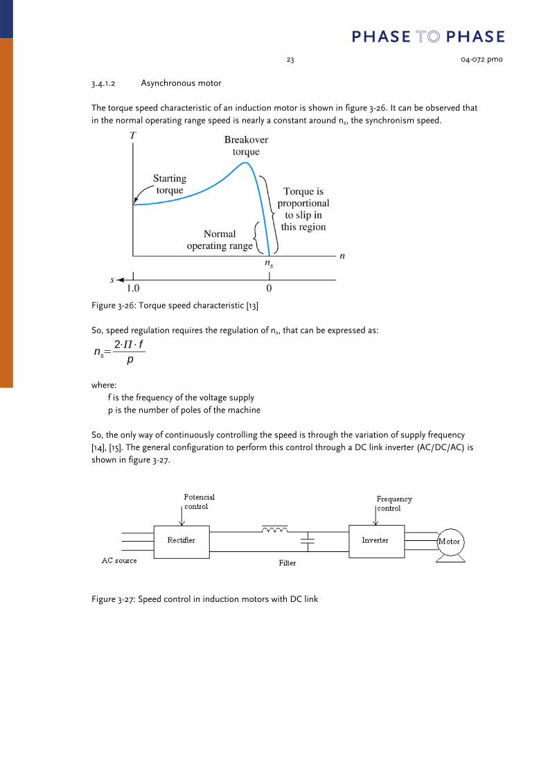
3.4.1.2 Asynchronous motor The torque speed characteristic of an induction motor is shown in figure 3-26. It can be observed that in the normal operating range speed is nearly a constant around ns, the synchronism speed.

Figure 3-26: Torque speed characteristic [13] So, speed regulation requires the regulation of ns, that can be expressed as:

ns2 f

p where: f is the frequency of the voltage supply p is the number of poles of the machine So, the only way of continuously controlling the speed is through the variation of supply frequency [14], [15]. The general configuration to perform this control through a DC link inverter (AC/DC/AC) is shown in figure 3-27.

Figure 3-27: Speed control in induction motors with DC link

24 04-072 pmo

In figure 3-28, the most used configurations are shown.

Figure 3-28: Most used configurations of AC/DC/AC converter for motor drives; (a) DC current intermediate circuit;

(b) Controlled DC voltage; (c) DC voltage-Chopped controlled; (d) PWM frequency converter

Lately, the development of new types of converters has allowed building these drives without DC link. Cycloconverters and matrix converters are used to control both voltage and frequency of the supply (figure 3-29). In figure 3-30, a cycloconverter is shown.

Figure 3-29: Speed control in induction motors without DC link

25 04-072 pmo

Figure 3-30: Cycloconverter induction motor drive The control of induction motor drives has to be both of voltage and frequency to avoid the saturation of the machine for the increase of the magnetic flux. This type of control is known as VVVF (variable frequency, variable voltage) and can be done in several ways. Scalar control or Volts/Hz control is the most usual one. For frequencies under the nominal one, it is necessary to decrease in the same rate the supply voltage to avoid the increase of the machine flux. For frequencies over the nominal one, it is not possible to keep constant the flux because voltage cannot be over the nominal. That means that to achieve speeds over the base speed is necessary to reduce the flux and that implies that the torque is also reduced. See figure 3-29. This is the simplest way of control. Only when great precision is required, it is not enough and other methods are needed as Vector or field orientation control (FOC), Direct torque and flux control (DTC), Instantaneous power control (IPC).

Figure 3-31: U/f relation when speed control is performed [16] Another alternative way of electronically controlling an induction motor is through energy recovery. It is based in that slip power which is wasted in the rotor as rotor copper losses and can be recovered through auxiliary devices. The slip frequency power is fed back to the supply after frequency conversion (figure 3-32). So, speed and power factor of the motor are adjusted by controlling value and phase of the slip frequency electromotive force.

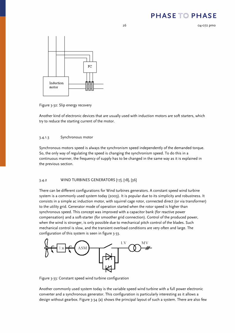
26 04-072 pmo

Figure 3-32: Slip energy recovery Another kind of electronic devices that are usually used with induction motors are soft starters, which try to reduce the starting current of the motor. 3.4.1.3 Synchronous motor Synchronous motors speed is always the synchronism speed independently of the demanded torque. So, the only way of regulating the speed is changing the synchronism speed. To do this in a continuous manner, the frequency of supply has to be changed in the same way as it is explained in the previous section. 3.4.2 WIND TURBINES GENERATORS [17], [18], [36] There can be different configurations for Wind turbines generators. A constant speed wind turbine system is a commonly used system today (2003). It is popular due to its simplicity and robustness. It consists in a simple ac induction motor, with squirrel cage rotor, connected direct (or via transformer) to the utility grid. Generator mode of operation started when the rotor speed is higher than synchronous speed. This concept was improved with a capacitor bank (for reactive power compensation) and a soft-starter (for smoother grid connection). Control of the produced power, when the wind is stronger, is only possible due to mechanical pitch control of the blades. Such mechanical control is slow, and the transient overload conditions are very often and large. The configuration of this system is seen in figure 3-33.

Figure 3-33: Constant speed wind turbine configuration Another commonly used system today is the variable speed wind turbine with a full power electronic converter and a synchronous generator. This configuration is particularly interesting as it allows a design without gearbox. Figure 3-34 (a) shows the principal layout of such a system. There are also few

27 04-072 pmo

examples of using an induction generator with a gearbox and a full power electronic converter but they are uncommon. Other possible configuration is the variable speed turbine with a doubly fed induction generator (shown in figure 34 (b)), which is likely to be one of the dominant systems in the near future. A frequency converter directly controls the currents in the rotor windings. This enables control of the whole generator output, using a PE converter, rated at 20-30% of nominal generator power which is cheaper than using a full converter.

Figure 3-34: Variable speed wind turbines:

(a) full power electronic converter and synchronous generator, (b) doubly-fed induction generation.

3.5 Devices for HVDC [19] THE HVDC (HIGH VOLTAGE DIRECT CURRENT) TECHNOLOGY [20], [21] The fundamental process that occurs in an HVDC system is the conversion of electrical current from AC to DC (rectifier) at the transmitting end, and from DC to AC (inverter) at the receiving end. There are three ways of achieving this conversion:

• Natural Commutated Converters: they are most used in the HVDC systems of today. The component that enables this conversion process is the thyristor, which is a controllable semiconductor that can carry very high currents (4000 A) and is able to block very high voltages (up to 10 kV). By means of connecting the thyristors in series it is possible to build up a thyristor valve, which is able to operate at very high voltages (several hundred of kV). The thyristor valve is operated at net frequency (50 Hz or 60 Hz) and by means of a control angle it is possible to change the DC voltage level of the bridge. This ability is the way by which the transmitted power is controlled rapidly and efficiently.

• Capacitor Commutated Converters (CCC). An improvement in the thyristor-based commutation, the CCC concept is characterized by the use of commutation capacitors inserted in series between the converter transformers and the thyristor valves. The commutation capacitors improve the commutation failure performance of the converters when connected to weak networks.

• Forced Commutated Converters or Self-Commutated Converters. This type of converters introduces a spectrum of advantages, e.g. feed of passive networks (without generation), independent control of active and reactive power, power quality. The valves of these converters are built up with semiconductors with the ability not only to turn-on but also to

28 04-072 pmo

turn-off. Two types of semiconductors are normally used in the forced commutated converters: the GTO (Gate Turn-Off Thyristor) or the IGBT (Insulated Gate Bipolar Transistor). Both of them have been in frequent use in industrial applications since early eighties. This kind of converter can be voltage source converter (VSC) or current source converter (CSC) depending on if the DC magnitude that is more and less constant is the voltage or the current. In HVDV applications only VSC are used. The VSC commutates with high frequency (not with the net frequency). The operation of the converter is achieved by Pulse Width Modulation (PWM). With PWM it is possible to create any phase angle and/or amplitude (up to a certain limit) by changing the PWM pattern, which can be done almost instantaneously. Thus, PWM offers the possibility to control both active and reactive power independently. This makes the PWM Voltage Source Converter a close to ideal component in the transmission network. From a transmission network viewpoint, it acts as a motor or generator without mass that can control active and reactive power almost instantaneously.

The Advantages of HVDC transmission are:

• More power can be transmitted per conductor per circuit

• Use of Ground Return Possible

• Smaller Tower Size

• Higher Capacity available for cables

• No skin effect

• Less corona and radio interference

• No Stability Problems

• Asynchronous interconnection possible

• Lower short circuit fault levels

• Tie line power is easily controlled Inherent problems associated with HVDC transmission are:

• Expensive converters.

• Reactive power requirement (in the case of natural commutated converters)

• Generation of harmonics

• Difficulty of circuit breaking

• Difficulty of voltage transformation

• Difficulty of high power generation

• Absence of overload capacity TWELVE PULSE VALVE GROUP One of the most used converters in HVDC is the natural commutated converter, which works using thyristor valves. Nearly all HVDC power converters with thyristor valves are assembled in a converter bridge of twelve-pulse configuration. Figures 3-35 demonstrate the use of two three-phase converter transformers with one DC side winding as an ungrounded star connection and the other a delta configuration. Consequently the AC voltages applied to each six pulse valve group which make up the twelve pulse valve group have a phase difference of 30 degrees which is utilized to cancel the AC side 5th and 7th harmonic currents and DC side 6th harmonic voltage, thus resulting in a significant saving in harmonic filters.

29 04-072 pmo

Figure 3-35: 12-pulse converter unit graphical symbol CLASSIFICATION OF DC LINKS DC links are classified into monopolar, bipolar and homopolar. In the case of the monopolar link (figure 3-36) there is only one conductor and the ground serves as the return path. The link normally operates at negative polarity as there is less corona loss and radio interference is reduced. The bipolar links have two conductors, one operating at positive polarity and the other operating at negative polarity. The junction between the two converters may be grounded at one or both ends. The ground does not normally carry current. However, if both ends are grounded, each link could be independently operated when necessary. This is shown in figure 3-37. The homopolar links, shown in figure 3-38, have two or more conductors having the same polarity (usually negative) and always operate with ground path as return.

Figure 3-38: Monopolar link

Figure 3-37: Bipolar link

30 04-072 pmo

Figure 3-36: Homopolar link 4 MODELING As a common characteristic, all electronic devices are very sensitive to great currents and under and over voltages. That means that all of them are protected against short circuits. So, as a first approximation it is possible to consider that electronic devices are switched off when a fault occurs and they do not add to the level of short circuit. However, more research has to be done in this field. 4.1 TCSC (Thyristor controlled series compensator) According to the literature [23][24], there are basically to ways of introducing these devices (figure 3-4) into load flow calculation:

• Total susceptance power flow model: in practice, the TCSC can be seen as an adjustable susceptance (Figure 4-1) that represents the fundamental frequency equivalent susceptance of the TCSC which value is determined by means of Newton-Raphson' s method in order to constrain the power flow across the branch to a specified value.

Figure 4-1: Variable series susceptance If the susceptance (or his inverse, the impedance X) is included as state variable into the method, the new Jacobian matrix for the element is shown above [23]:

31 04-072 pmo

Once the reactance, which provides the desired power flow across the branch is calculated, it is possible to find the firing angle of the thyristor. To do this, an expression for the equivalent impedance of the TCSC depending on the value of the firing angle is needed. The most simple and used one is:

XTCSC

X C X L

X L

XC 2 sin 2

where a can be between 90 and 180 degrees. But this expression has been claimed [25] to be inexact near the resonance point because it does not consider the loop current between the reactor and the capacitor. A more complex equation is given to solve this problem:

XTCSC XC C1 2 sin 2

C2cos2 tan tan

where:

X LC

XC X L

XC X L;

C1

X C X LC ;

C2 4X LC

2

X L;

• Firing angle power flow model: in order to avoid the extra iterative process that would be necessary using the total susceptance model to find the firing angle, this model includes the firing angle as one of the state variables. So the Jacobian matrix is shown above [23]:

32 04-072 pmo

However, to avoid numerical problems as a result of ill conditioning of the Jacobian matrix, some works [25][26] recommend to treat the TCSC as a fixed reactance until a specified voltage angle difference appears across the reactance. From then on, the control equations of the series compensator are included in the iterative process. But, both methods require a modification in the Jacobian matrix used in Vision. A way of proceeding similar to the one used in Vision to find the position of the tap changers of transformers could be effective in this problem to avoid the changes in the Jacobian matrix. The TCSC and the line where it is installed can be seen as a line with variable impedance. The objective of installing the TCSC is to get the power flow through the line (between nodes i and j) equal to the specified value (Pij

esp). Firstly, the power flow is calculated with the original impedance (X) of the line. If the power flow through the line (Pij

calc) is equal to Pijesp , the problem is solved and the installation of the TCSC is not

necessary. Otherwise, the impedance of the line must be altered. The equation that controls the power flow if the line is mainly inductive is:

Pij

Vi V j

X eqsin ij

So, if Pij

calc > Pijesp, Xeq of the line must be increased

Pijcalc < Pij

esp, Xeq of the line must be decreased where

TCSClineeq XXX +=

Then, the new power flow is calculated and the process continues until Pij

calc =Pijesp. According to [27],

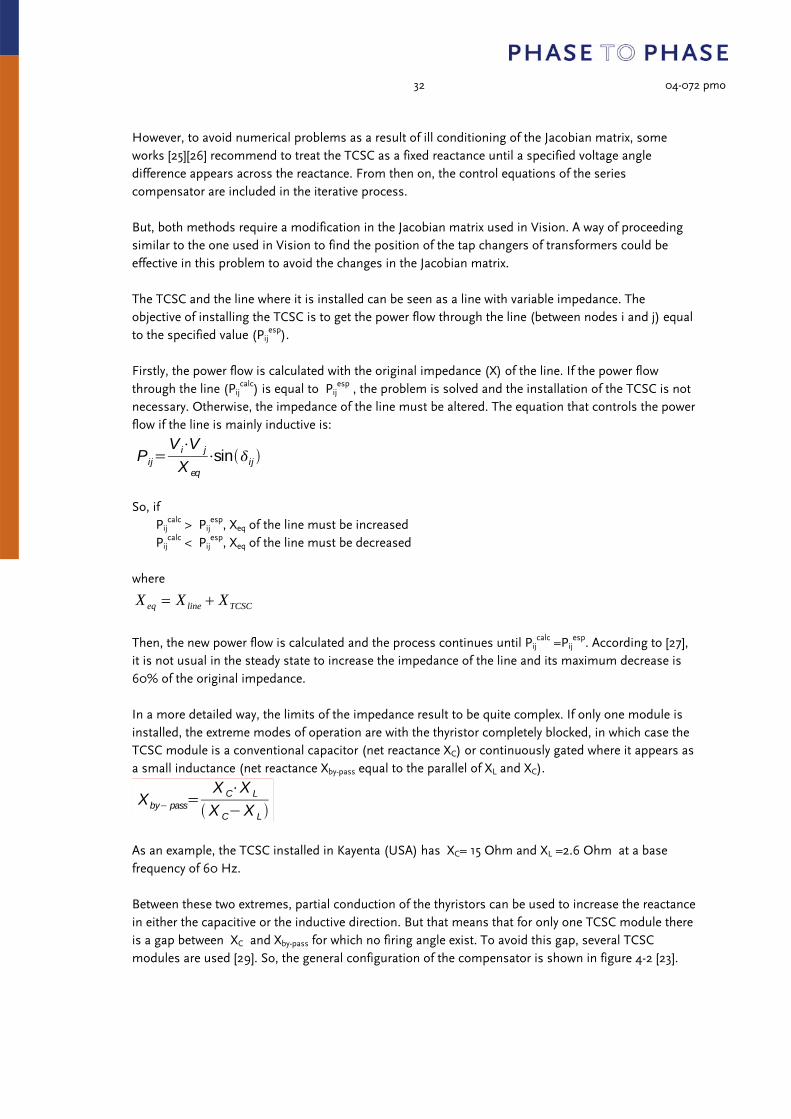
it is not usual in the steady state to increase the impedance of the line and its maximum decrease is 60% of the original impedance. In a more detailed way, the limits of the impedance result to be quite complex. If only one module is installed, the extreme modes of operation are with the thyristor completely blocked, in which case the TCSC module is a conventional capacitor (net reactance XC) or continuously gated where it appears as a small inductance (net reactance Xby-pass equal to the parallel of XL and XC).

Xby pass

X C X L

X C X L

As an example, the TCSC installed in Kayenta (USA) has XC= 15 Ohm and XL =2.6 Ohm at a base frequency of 60 Hz. Between these two extremes, partial conduction of the thyristors can be used to increase the reactance in either the capacitive or the inductive direction. But that means that for only one TCSC module there is a gap between XC and Xby-pass for which no firing angle exist. To avoid this gap, several TCSC modules are used [29]. So, the general configuration of the compensator is shown in figure 4-2 [23].

33 04-072 pmo

Figure 4-2: TCSC configuration Then, the limits for the multimodule TCSC reactance depending on the line current are shown in figure 4-3 [29]. In the figure, all the reactances are in per unit on XC what means that the capacitive region corresponds to the positive reactance.

Figure 4-3: Multimodule TCSC equivalent reactance The limits are:

• maximum inductive (Xmin0) and capacitive reactance (Xmax0) due to the limitations in the firing angle

• maximum voltage across the device in the capacitive and in the inductive region

• maximum current through the device. If the current is over this maxim, the TCSC will go into the protective mode with Xby-pass. So, this is the reactance that has to be considered in fault calculations.

As a first test for this method, a macro of Vision (see annex) has been used to control the power flow between Holland and Germany through the line between Meeden and Diele. In this first attempt, there has not been considered the limits in the equivalent impedance. The original power flow in the line

34 04-072 pmo

was 97.74MW and the specified values have been 150MW, 125MW, and 100MW. The calculation process can be seen in figure 4-4, 4-5, 4-6.

75 100 125 150 175 200 225-6-5-4-3-2-1012345678

Calculation process for 150 MW

Power Flow (MW)

Equ

ival

ent I

mpe

danc

e (o

hm)

Figure 4-4: Calculation process for 150MW

95 100 105 110 115 120 125 130 135 1400.5

11.5

22.5

33.5

44.5

55.5

66.5

77.5

Calculation Process for 125MW

Power Flow (MW)

Equ

ival

ent I

mpe

danc

e(oh

ms)

Figure 4-5: Calculation process for 125 MW

35 04-072 pmo

97.5 98 98.5 99 99.5 100 100.56.856.9

6.957

7.057.1

7.157.2

7.257.3

7.357.4

7.457.5

Calculation Process for 100 MW

Power Flow(MW)

Equ

ival

ent I

mpe

danc

e (o

hm)

Figure 4- 6: Calculation process for 100 MW In the first iteration, the increase or decrease of the equivalent impedance has been calculated as the difference between the desired power flow and the calculated power flow multiplied by a factor (0.01)

in order to get a small ΔX and be able to obtain a good approximation of the derivate of P in respect to

X through this ΔX. In the iteration i, this derivate is approximate by:

Pi 1 Pi

Xi

PX

And the next increase or decrease of the impedance is calculated as:

Xi 1Pi

Pi 1 Pi

X i

As a final remark, it has to be considered that this way of controlling power flow is recommended in transportation networks because in distribution the control is not so easy. 4.2 TCPAR (Thyristor Control Phase Angle Regulator) The steady state analysis of the TCPAR is the same as the traditional phase-angle regulating transformer. The only difference is that the electronic one can provide the control of load flow quicker than the mechanical one. So, in load flow studies, it is possible to use the same model for both [28]. These devices can be represented as transformers in which the turn ratio is a complex value:

r mej

where m is the relation in the magnitude of the voltage. This can be:

• m 1 for phase shifting transformers. They just shift the voltage but do not change the magnitude (see figure 4-7).

36 04-072 pmo

Figure 4-7: Phase Shifter

• m 1 j for quadrature booster. They shift the voltage by means of injecting a series voltage in quadrature with the line voltage (figure 4-8). In this case, both magnitude and angle of the voltage are changed.

Figure 4-8: Quadrature Booster Whatever of this cases is being analyzed, the leakage reactance of the transformer change as follows

Z Rser jX sersin

sin max

2

Rsht jX sht

where: Rser, Xser are the leakage resistance and reactance of the series winding Rsht, Xsht are the leakage resistance and reactance of the shunt winding

αmax is the maximum phase shift angle As with the TCSC, the purpose to introduce the TCPAR in a branch is the control of the active power that goes through it.

37 04-072 pmo

In [28], to get this control it is recommended to introduce the phase shift of the transformer as a state variable. The new equation is then added into the Newton-Raphson algorithm is the one that express the power flow between nodes k and m in relation to the state variables. In order to avoid the change in the Jacobian matrix, a similar way of processing as in case of the TCSC is done. The desired power flow between nodes i and j, can be noted as Pijesp. Firstly, the power flow is calculated without any phase shift. If the power flow through the line (Pijcalc) is equal to Pijesp , the problem is solved. Otherwise, some phase shift has to be introduced. The equation that controls the power flow if the line is mainly inductive is:

Pij

Vi V j

X eqsin ij

where δij is the phase shift that is produced by the phase shifting of the transformer ( αij ) and also the one produced by the reactances of the transformer. So, if

Pijcalc > Pij

esp, the phase shift αij must be increased.

Pijcalc < Pij

esp,the phase shift αij must be decreased. Then, the new power flow is calculated and the process continues until Pij

calc =Pijesp.

According to [28], the limits that must be taken into account are:

• αmax : maximum phase shift

• αmin : minimum phase shift

• the MVA through the electronic device must be lower or equal to the nominal MVA. The apparent power through the thyristor device can be expressed in function of the apparent power through the branch as follows: [29]

Sdevice 2Sbranch sin2

Finally, it has to be taken into account that the phase shift can only vary in a discrete way and so the tap size in degrees has to be considered. As a first try of this procedure, a phase shifter transformer has been implemented in Vision in the high voltage line between Meeden and Diele in the border between Germany and the Netherlands (see annex). The initial power flow through this line is 97.923 MW and the specified power has been set in 150MW, 125MW and 100MW. The calculation process is shown in figure 4-9, 4-10 and 4-11 respectively.

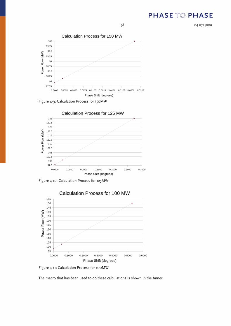
38 04-072 pmo

0.0000 0.0025 0.0050 0.0075 0.0100 0.0125 0.0150 0.0175 0.0200 0.0225

97.75

98

98.25

98.5

98.75

99

99.25

99.5

99.75

100

Calculation Process for 150 MW

Phase Shift (degrees)

Pow

er F

low

(MW

)

Figure 4-9: Calculation Process for 150MW

0.0000 0.0500 0.1000 0.1500 0.2000 0.2500 0.3000

97.5

100

102.5

105

107.5

110

112.5

115

117.5

120

122.5

125

Calculation Process for 125 MW

Phase Shift (degrees)

Pow

er F

low

(MW

)

Figure 4-10: Calculation Process for 125MW

0.0000 0.1000 0.2000 0.3000 0.4000 0.5000 0.600095

100105110115120125130135140145150155

Calculation Process for 100 MW

Phase Shift (degrees)

Pow

er F

low

(MW

)

Figure 4-11: Calculation Process for 100MW The macro that has been used to do these calculations is shown in the Annex.

39 04-072 pmo

The way of finding the increases or decreases of the phase shift is similar to the used to calculate the impedance variations in the TCSC. As in this case, it is necessary to consider that it is only valid for transportation networks. In the first iteration, the increase or decrease of the phase shift has been calculated as the difference between the desired power flow and the calculated power flow multiplied by a factor (0.001) in order

to get a small Δα and be able to obtain a good approximation of the derivate of P in respect to α

through this Δα. In the iteration i, this derivate is approximate by:

Pi 1 Pi

i

P

And the next increase or decrease of the impedance is calculated as:

i 1Pi

Pi 1 Pi

i

If the results obtained in the power flow control through a TCSC and a TCPAR are compared, it seems that the TCPAR is more effective and the calculation process is quicker. 4.3 BESS (Battery Energy Storage System) The usual configuration of a Battery Energy Storage System (BESS) is shown in figure 4-12.

Figure 4-12: BESS general configuration

40 04-072 pmo

A BESS can operate in three different modes: isolated from the utility in an emergency situation, resynchronizing to the utility after an emergency situation and on utility. The last one is the normal mode of operation and the only that is within the scope of this work. In this situation, the terminal voltage (Vt ) is given by the network and the active power for the loads is supplied by the grid. The BESS is charging or peak shaving and managing reactive power for the loads. That means that the power conditioning system (PCS) has to provide bi-directional power conversion between AC and DC side both active and reactive power and so the BESS can operate in the four quadrants shown in figure 4-13 with the only constraints of the thermal rating of the converter (with some overload capability for limited periods of time) and the available battery voltage.

Figure 4-13: Quadrants of operation of a BESS In general, the BESS control system is designed to emulate a classical synchronous machine. The equivalent circuit is shown in figure 4-14 [29][30], where Xt represents the transformer reactance.

Figure 4-14: BESS equivalent Circuit Since the generated voltage is completely controllable, the AC current can be supplied at any phase angle relative to the terminal voltage (VT). In steady state situations, the only constraint that has to be taken into account is the maximum current that can flow through the converter because the limits of the internal voltage (Vi) are not so restrictive. So, in the phasor diagram in figure 4-15 the possible points of operation can be seen.

41 04-072 pmo

Figure 4-15: Phasor Diagram of the BESS And the expressions of the active and reactive power given by the BESS to the network are:

PVi V t

Xsen

QV i V t

Xcos

Vt2

XVt

V i cos V t

XV t

Vi ' V t

XV t I Q

where Vi' is the horizontal projection of the internal voltage

)cos(' δii VV =

and the reactive current is:

I Q

Vi ' V t

X

To include this storage device into the load flow, [29][30] recommends its representation as a PV bus and a fictitious reactance as shown in figure 4-14. But this representation has some discrepancies with the V-IQ characteristic of a STATCOM in the limits of the device because the PV node representation implies that the limit is set by Q and not by I as is shown in figure 4-16. As explained in [29], the behaviour of the BESS with respect to reactive power is the same of a STATCOM if you take into account Vi' and not Vi. That means that the same characteristic can be used for the BESS and the STATCOM. In this figure, the reactive current is positive when it is inductive and negative when it is capacitive. In the load flow the convention of sign is different and so the curve has to be changed. It is shown in figure 4-17 where the reactive current is positive if the device injects reactive power to the utility (as a capacitive element) and it is negative if it consumes reactive power from the network (inductive element).

42 04-072 pmo

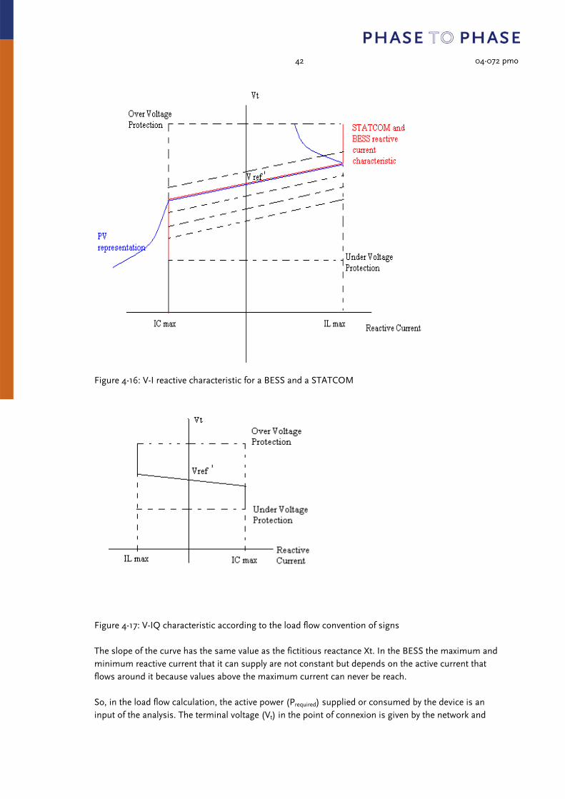
Figure 4-16: V-I reactive characteristic for a BESS and a STATCOM

Figure 4-17: V-IQ characteristic according to the load flow convention of signs The slope of the curve has the same value as the fictitious reactance Xt. In the BESS the maximum and minimum reactive current that it can supply are not constant but depends on the active current that flows around it because values above the maximum current can never be reach. So, in the load flow calculation, the active power (Prequired) supplied or consumed by the device is an input of the analysis. The terminal voltage (Vt) in the point of connexion is given by the network and

43 04-072 pmo

so, in each iteration of the process is also a known value. The reference voltage (Vi) with which the inverter is working is determined by the user. With these values, it is possible to calculate the maximum and minimum value of the reactive current (IQ) and also the value that corresponds to the terminal voltage (all values given in p.u.):

maxmax IVS t ⋅=

222QP III +=

I Q max I max2 Prequired

V t

2

I Q min I max2 Prequired

V t

2

Vi sen P XV t

Vi ' V i cos V i2 P X

V t

2

I Q required

V i ' Vt

X t

If the required IQ is within the limits, the BESS can be represented as a PQ node with:

P Prequired

Q Qrequired V t I Q required Otherwise, a correction is needed. The user has to decide which criterion must be applied in the correction: it is possible to maintain the power factor or the active power. If the power factor is maintained, the active and reactive power must be decrease in the same proportion until the maximum apparent power is reached and the BESS can be represented as a PQ node with:

P Prequired

Smax

Prequired2 Qrequired

2

Q Qrequired

Smax

Prequired2 Qrequired

2

It has to be noted that if this way of correction is chosen, the active power value specified by the user at the beginning of the calculation can change during the process. When the active power is maintained, the BESS is also represented as a PQ node but with the following values of P and Q depending if the violation is above IQ max :

44 04-072 pmo

maxmax Qt

required

IVQQ

PP

⋅==

=

or below IQ min :

minmin Qt

required

IVQQ

PP

⋅==

=

If the voltage that is determined by the network (Vt) is above the value in which the over voltage protection of the inverter is settled or under the value of the under voltage protection, the BESS is disconnected and so,

00

==

QP

In case that a shunt connected filter is used, for the load flow studies it can be modelled just as a simple shunt capacitor with its capacitance equal to the equivalent capacitance of the filter in the fundamental frequency. During the interpretation of the load flow results, the energy that is supplied to or by the battery has to be taken into account because the BESS has finite storage capabilities and so it cannot be charged infinitely nor give power infinitely. In fact, the amount of power that the battery can provide depends on how long this power has to be supplied. Finally, in short circuit calculation it is not necessary to consider BESS devices because the control of the device has to be designed to instantly switch off from the line when an over current or an under voltage in the line is detected. 4.4 STATCOM and SMESS The STACOM (Static Compensator) and the SMESS (Super Magnetic Energy Storage System) are shunt-connected devices. They both use voltage source converter (VSC) as the BESS to make the connection with the network as can be seen in figure 4-19 for the STATCOM and figure 4-18 for the SMESS.

Figure 4-19: SMESS Figure 4-18: STATCOM

45 04-072 pmo

The SMESS is able to provide active power just for a few seconds so it is used to mitigate voltage sags or brief interruptions of the supply. But in the steady state both the SMESS and the STATCOM are only able to provide or consume reactive power. So, their model is just a particular case of the BESS one with the active power equal to zero (P=0). So given the reference voltage and knowing the terminal voltage it is possible to find the Q provided by the device through the characteristic in figure 4-14. 4.5 SOFT STARTER When an induction motor is started directly on line, its current can achieve six times its nominal value. In big motors, that can cause disturbance in the network and voltage drops in the point of connexion of the machine. Moreover, in a start of this kind, the motor suffers a mechanical shock, which leads to a shortening of its life. For all this questions, it has been usual to soft the start of this kind of motors in mechanics and electro mechanics ways (starting transformer, star-delta transformer, variable rotor resistance,...). Nowadays, electronic devices are the most used ones in these applications. The current through the motor is proportional to the supplied voltage. So, a decrease in the voltage allows a decrease in the current of the same rate. The only problem is that the torque developed by the motor is proportional to the square of the voltage. That means, for example, that to reduce the starting current in a 50%, the starting torque decreases in a 75%. There can be applications in which this starting torque is not enough to make the motor move. In the case that a variable speed drive is used to allow speed control of the motor in its normal functioning, this same drive can be used to smooth the start of the machine supplying a voltage of reduced magnitude and frequency. But in most cases, the drive is not installed and so, a device is needed just to smooth the start. This is the device usually known as soft starter (figure 4-20).

Figure 4-20: Soft starter usual configuration It consists of an AC/AC converter in which the input and the output voltage has the same frequency and the magnitude of the output voltage is controlled by the phase cut principle. Firing the thyristors each time in a smaller angle as it is shown in figure 4-21 smoothly increases the magnitude of the voltage supplied to the motor during the start.

46 04-072 pmo

Figure 4-21: Phase cut principle of operation of the soft starter Once the motor has started, the contactor is closed and the thyristors are no longer fired (by-pass mode). That means that in load flow calculations in which the start of the motor is not considered, the soft starter has not to be taken into account. Equally, when a short circuit is being simulated when the motor is running, the thyristors are not conducting so they do not have to be considered. If the short circuit occurs when the motor is starting, the protections that most of the industrial motor starters have would stop the firing of the thyristors and prevent any damage on the device [31][32][33]. The soft starter can have different modes of operation:

• Current limiting starting: the user specification is the maximum current that it is allowed with respect to the nominal current of the motor. This mode can now be simulated in Vision through the specification Is/INom in the general dialog box of the asynchronous motor.

• Torque control: in some applications with high resistive starting torque, the current limiting starting makes the motor torque insufficient. To avoid this problem, the minimum required torque in the start with respect to the locked rotor torque is specified by the user. Then, the maximum current that is reached in the start can be approximate as [32]:

minimum

locked rotor

U L soft starter

U L

2

I soft starter

I Nom

I s

I Nom

U L soft starter

U L

I s

I Nom

minimum

locked rotor

47 04-072 pmo

and then the calculation is made in Vision with this new value of the rate between start current and nominal current of the motor.

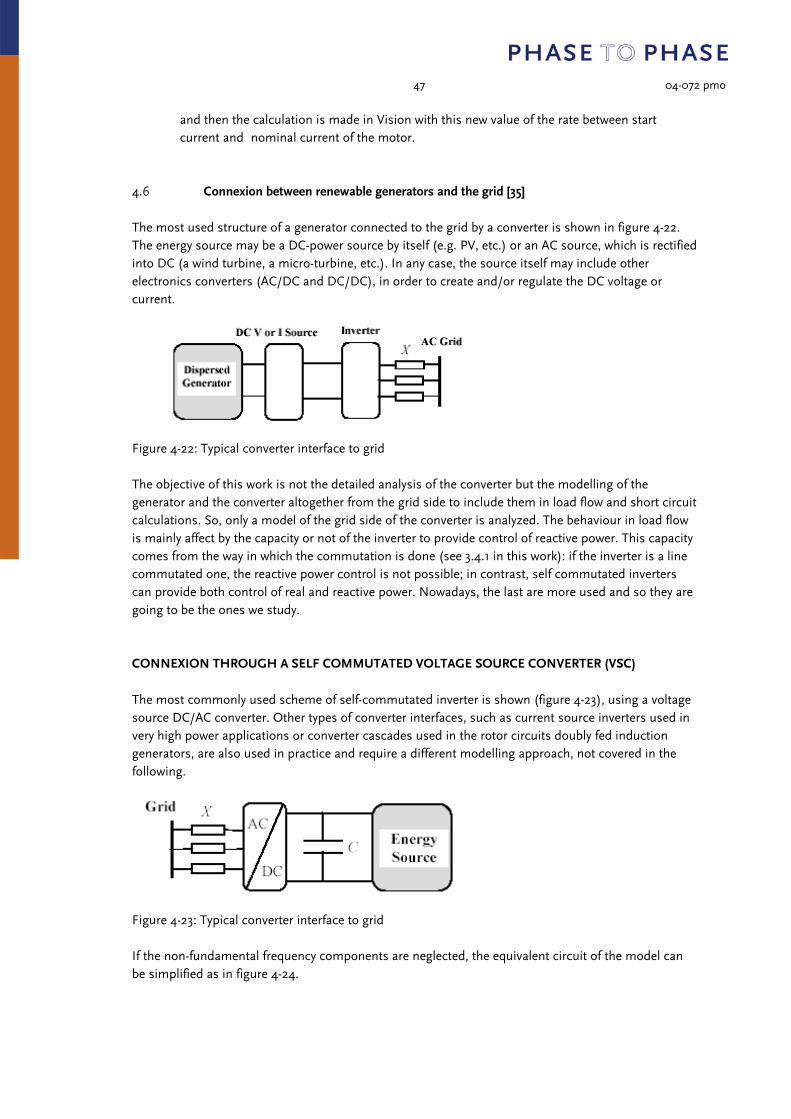
4.6 Connexion between renewable generators and the grid [35] The most used structure of a generator connected to the grid by a converter is shown in figure 4-22. The energy source may be a DC-power source by itself (e.g. PV, etc.) or an AC source, which is rectified into DC (a wind turbine, a micro-turbine, etc.). In any case, the source itself may include other electronics converters (AC/DC and DC/DC), in order to create and/or regulate the DC voltage or current.

Figure 4-22: Typical converter interface to grid The objective of this work is not the detailed analysis of the converter but the modelling of the generator and the converter altogether from the grid side to include them in load flow and short circuit calculations. So, only a model of the grid side of the converter is analyzed. The behaviour in load flow is mainly affect by the capacity or not of the inverter to provide control of reactive power. This capacity comes from the way in which the commutation is done (see 3.4.1 in this work): if the inverter is a line commutated one, the reactive power control is not possible; in contrast, self commutated inverters can provide both control of real and reactive power. Nowadays, the last are more used and so they are going to be the ones we study. CONNEXION THROUGH A SELF COMMUTATED VOLTAGE SOURCE CONVERTER (VSC) The most commonly used scheme of self-commutated inverter is shown (figure 4-23), using a voltage source DC/AC converter. Other types of converter interfaces, such as current source inverters used in very high power applications or converter cascades used in the rotor circuits doubly fed induction generators, are also used in practice and require a different modelling approach, not covered in the following.

Figure 4-23: Typical converter interface to grid If the non-fundamental frequency components are neglected, the equivalent circuit of the model can be simplified as in figure 4-24.

48 04-072 pmo

Figure 4-24: Fundamental frequency equivalent circuit and phasor diagram for the output converter If the resistance of connexion between the inverter and the network are neglected because it is quite small compared to the impedance, the following relations give the active and reactive power in the connection to the network:

PVi V b

X fsin

QV i V b

X fcos

V f2

X f

The active power P is predominantly dependent on the power angle δ between the inverter and grid voltage phasors, while Q is mainly determined by the inverter voltage magnitude Vi. This means that the behaviour is more or less the same of the BESS. However, when a renewable energy source is connected to the grid there are two different modes of operation:

• Constant Power Factor: it is a usual way of connection. Depending on the P that the source is given, the inverter set the reference voltage so that to get the Q that allows maintaining a constant power factor. So, in order to include it in Vision, it can be seen as a synchronous

generator with cos(ϕ) control. That means that given a Prequired and a cos(ϕ) set by the user, the element can be defined as a PQ node with:

P Prequired

Q QrequiredP

cos1 sen 2

However, the constraints about the maximum current through the inverter must be taken into account. In the case that:

IPrequired

2 Qrequired2

VtI max

a correction is needed. In order to maintain the same power factor, P and Q must decrease in the same way:

P Prequired

V t I max

Prequired2 Qrequired

2

Q QrequiredVt I max

Prequired2 Qrequired

2

49 04-072 pmo

• Bus Voltage Regulation: another possibility of connexion is to set the reference voltage of the inverter to regulate the voltage in the point of connexion. The inverter would give the necessary Q to do so. This way of operation is similar to the BESS operation. So, the inputs of the analysis are the active power (P) and the reference voltage of the inverter (Vi). As the networks determine the voltage of the bus (Vb) this is also a known value. With all this, it is possible to find the reactive power that the inverter has to supply using the same characteristic as the BESS:

Figure 4-25: V-IQ characteristic for a renewable energy source connected to the grid through a VSC

Vi ' V i cos V i2 P X f

V t

2

I Q required

V i ' Vt

X f

As always, the current through the inverter must be within the limits. That means, that the reactive current has to be between:

I Q max I max2 Prequired

V b

2

I Q min I max2 Prequired

V b

2

Otherwise, it is necessary to correct this value. In this case, seems more reasonable to keep the same active power and reduce the reactive current until the limit so that the new Q is:

minmin Qb IVQQ ⋅==

or

maxmax Qb IVQQ ⋅==

depending on which limit has been violated.

50 04-072 pmo

Finally, it has to be considered that motor drives are not included in this model because the grid side converter is usually a non-controlled rectifier or a thyristor rectifier. This model is only valid for the devices connected to the grid through a voltage source converter (VSC) with self-commutated switches. 5 CONCLUSIONS In this project a limited study is carried out on the suitable models of electronic devices used in power systems for their inclusion in Vision. First, a classification of the most important devices has been made according to their function and not so extensively in how there are inside. After this, some models are presented.

• All the energy sources (wind turbines, photo voltaic arrays, fuel cells,...), storages (batteries, superconducting magnets,...) and even shunt static compensator (STATCOM and D-STATCOM) connected to the grid through a voltage source converter (VSC) can be modelled in the same way for the steady state analysis. They can be seen as a voltage source connected to the network through a reactance.

• The FACTS devices as TCSC and TCPAR can be modelled in load flow calculations as a variable impedance and a phase shifter transformer respectively to get the desired power flow in the branch where they are installed.

• Soft Starters for induction motors only have to be considered in motor start calculations and they just make a change in the ratio between starting and nominal current.

After the project some questions remain open:

• More research is needed about the behaviour of these devices in fault situations. They are all well protected but some of them have an active role in reducing short circuit levels that has to be studied deeply.

• No model is given here for motor drives from the network side because of the limited time. The general model of VSC is not suitable because the line side converter of motor drives is, in general, a non-controlled or a thyristor rectifier, not a self-commutated one.

• Energy sources connected to the network not through a VSC but, for example, through a current source inverter or a line-commutated inverter are not modelled here. A model for doubly fed induction generators used in wind energy is neither given.

• We have only provided models for some of the FACTS and Custom Power devices but, in general, the methodology is similar to the used for TCSC and TCPAR. Moreover, general models for the rest of these devices are available in the literature. See references [26], [28], [29] and [30].

• It is not explicit in this report but the VSC model can be used to represent DC transmissions. Then, the equations of the DC line and the constraints that they imply to the power in both sides of the line must be taken into account.

51 04-072 pmo

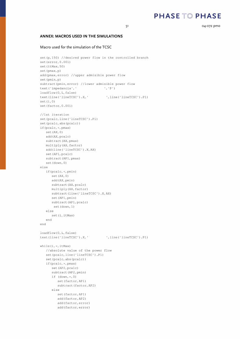
ANNEX: MACROS USED IN THE SIMULATIONS Macro used for the simulation of the TCSC set(p,150) //desired power flow in the controlled branch set(error,0.001) set(itMax,50) set(pmax,p) add(pmax,error) //upper admisible power flow set(pmin,p) subtract(pmin,error) //lower admisible power flow text('impedancia',' ','P') loadflow(0,L,false) text(line('lineTCSC').X,' ',line('lineTCSC').P1) set(i,0) set(factor,0.001) //1st iteration set(pcalc,line('lineTCSC').P1) set(pcalc,abs(pcalc)) if(pcalc,>,pmax) set(AX,0) add(AX,pcalc) subtract(AX,pmax) multiply(AX,factor) add(line('lineTCSC').X,AX) set(AP1,pcalc) subtract(AP1,pmax) set(down,0) else if(pcalc,<,pmin) set(AX,0) add(AX,pmin) subtract(AX,pcalc) multiply(AX,factor) subtract(line('lineTCSC').X,AX) set(AP1,pmin) subtract(AP1,pcalc) set(down,1) else set(i,itMax) end end loadflow(0,L,false) text(line('lineTCSC').X,' ',line('lineTCSC').P1) while(i,<,itMax) //absolute value of the power flow set(pcalc,line('lineTCSC').P1) set(pcalc,abs(pcalc)) if(pcalc,>,pmax) set(AP2,pcalc) subtract(AP2,pmin) if (down,=,0) set(factor,AP1) subtract(factor,AP2) else set(factor,AP1) add(factor,AP2) add(factor,error) add(factor,error)

52 04-072 pmo

divide(AX,factor) end divide(factor,AX) set(AX,AP2) add(line('lineTCSC').X,AX) set(AP1,pcalc) subtract(AP1,pmax) set(down,0) else if(pcalc,<,pmin) set(AP2,pmin) subtract(AP2,pcalc) if (down,=,1) set(factor,AP1) subtract(factor,AP2) else set(factor,AP1) add(factor,AP2) add(factor,error) add(factor,error) end divide(factor,AX) set(AX,AP2) divide(AX,factor) subtract(line('lineTCSC').X,AX) set(AP1,pmin) subtract(AP1,pcalc) set(down,1) else set(i,itMax) end end add(i,1) loadflow(0,L,false) text(line('lineTCSC').X,' ',line('lineTCSC').P1) end Macro used for the simulation of the TCPAR set(p,150) //desired power flow in the controlled branch set(error,1e-6) set(itMax,200) set(pmax,p) add(pmax,error) //upper admisible power flow set(pmin,p) subtract(pmin,error) //lower admisible power flow text('desfase',' ','P') loadflow(0,L,false) text(transformer('PhShTr').PhaseShift,' ',transformer('PhShTr').P1) set(i,0) set(factor,0.001) //1st iteration set(pcalc,transformer('PhShTr').P1) set(pcalc,abs(pcalc)) if(pcalc,>,pmax) set(APh,0) add(APh,pcalc) subtract(APh,pmax) multiply(APh,factor) subtract(transformer('PhShTr').PhaseShift,APh)

53 04-072 pmo

set(AP1,pcalc) subtract(AP1,pmax) set(down,0) else if(pcalc,<,pmin) set(APh,0) add(APh,pmin) subtract(APh,pcalc) multiply(APh,factor) add(transformer('PhShTr').PhaseShift,APh) set(AP1,pmin) subtract(AP1,pcalc) set(down,1) else set(i,itMax) end end loadflow(0,L,false) text(transformer('PhShTr').PhaseShift,' ',transformer('PhShTr').P1) while(i,<,itMax) //absolute value of the power flow set(pcalc,transformer('PhShTr').P1) set(pcalc,abs(pcalc)) if(pcalc,>,pmax) set(AP2,pcalc) subtract(AP2,pmin) if (down,=,0) set(factor,AP1) subtract(factor,AP2) else set(factor,AP1) add(factor,AP2) add(factor,error) add(factor,error) end divide(factor,APh) set(APh,AP2) divide(APh,factor) subtract(transformer('PhShTr').PhaseShift,APh) set(AP1,pcalc) subtract(AP1,pmax) set(down,0) else if(pcalc,<,pmin) set(AP2,pmin) subtract(AP2,pcalc) if (down,=,1) set(factor,AP1) subtract(factor,AP2) else set(factor,AP1) add(factor,AP2) add(factor,error) add(factor,error) end divide(factor,APh) set(APh,AP2) divide(APh,factor) add(transformer('PhShTr').PhaseShift,APh) set(AP1,pmin) subtract(AP1,pcalc)

54 04-072 pmo

set(down,1) else set(i,itMax) end end add(i,1) loadflow(0,L,false) text(transformer('PhShTr').PhaseShift,' ',transformer('PhShTr').P1) end

55 04-072 pmo

REFERENCES [1] Martinez Velasco, J.A. “Sistemas eléctricos de Potencia “ CPDA (1994). [2] El-Hawary, M. “Electrical Power Systems: Design and Analyisis”, 1995, IEEE. [3] Wadhwa, “Electrical Power Systems”, 1991, 2nd Edition Ed. John Wiley. [4] Help of VISION. [5] Calvas, R., Noblat, B., Ducluzaux, A., Thomasset, G. “Calculation of short circuit currents”, Cahier Technique Merlin Gerin n°158. [6] Martinez Velasco, J.A.”Sistemas flexibles de transporte y distribucion de energía eléctrica”, Energía p.85-92. [7] Hirvonen, R. “Introduction to FACTS”, Helsinki University of Technology. [8] Kyyrä, J. “Power Electronics in FACTS”, Helsinki University of Technology. [9] de Mattos Tenório, A.R., Gama, C.A. “Resolvendo problemas de ressonância subsíncrona através do TCSC e do dispositivo NGH – análise de estratégias de controle”, XV Seminário Nacional de Produção e Transmissão de Energia Eléctrica. [10] Anaya-Lara, O. and Acha, E., “Modeling and Analysis of Custom Power Systems by PSCAD/EMTDC”, IEEE Transactions on Power Delivery, vol.17, no 1, January 2002. [11] http://www.ece.umr.edu/links/power/Energy_Course/energy/facts/cp.htm. [12] Salam, Z. “Power Electronics and Drives “, UTMJB. [13] Still, A.M. “AC Motors”,2002, “Electrical Machines and Information Technology Systems”, USNA. [14] Chattopadhyay, A.K. “High Power High Performance Industrial AC Drives- A technology review” (2003), Department of Electrical Engineering Bengal Engineering College. [15] Penrose, H.W., “Motor System Troubleshooting: Evaluating Motor and Drive Installation Issues”, All Test Pro, BJM Corp. [16] AB Drives, “Frequency controlled AC motor drive”. [17] Hansen L. H., Helle L., Blaabjerg F., Ritchie E., Munk-Nielsen S., Bindner H., Sørensen P. and Bak-Jensen B. “Conceptual survey of Generators and Power Electronics for Wind Turbines”, Risø National Laboratory, Roskilde, Denmark, December 2001. [18] Schreiber, D, “State of the Art of Variable Speed Wind Turbines”, 11th International Symposium on Power Electronics - Ee 2001. [19] Wood A., “Current sourced HVDC. An introduction”,University of Canterbury, Christchurch, New Zeland. [20] Rudervall R., Charpentier J. P. and Sharma R., “High Voltage Direct Current (HVDC) Transmission Systems Technology Review Paper”, Presented at Energy Week 2000, Washington, D.C, USA, March 7-8, 2000. [21] Rohan Lucas, J., “High Voltage Engineering”, Department of Electrical Engineerig, University of Moratuwa, Sri Lanka, 2001. [22] University of Iceland, “Models for Transmission Lines and Transmission Capacity with HVAC, HVDC and Cables”. [23] Venegas, T., Fuerte-Esquivel, R., “Steady-State Modeling of an Advanced Series Compensator for Power Flow Analysis of Electric Networks in Phase Co-Ordinates”, IEEE Transactions on Power Delivery, Vol. 16, no 4, October 2001. [24] Geidl, M., “Implementation of FACTS and Economic Generation Dispatch in an Interactive Power Flow Simulation Platform”, ETH Zürich. [25] Fuerte-Esquivel, C.R., Acha, E., Ambriz-Pérez, H., “A Thyristor Controlled Series Compensator Model for the Power Flow Solution of Practical Power Electronic”, IEEE Transactions on Power Systems, Vol. 15, no 1, February 2000. [26] Arrillaga, J., Watson, N.R., “Computer Modeling of Electrical Power Systems”, 2001, 2nd Edition, Ed.Wiley.

56 04-072 pmo

[27] Faimuenway, S., Jiriwipakorn,S., Bunjognjit, S., Krisnachinda, N., “TCSC as a tool to reduce the transmission congestion charge”, CI RED 17th International Conference on Electricity Distribution Barcelona, 12-15 May 2003 [28] Fuerte-Esquivel, C.R., Acha. E., “Newton-Raphson algorithm for the reliable solution of large power networks with embedded FACTS devices”, IEE Proc.-Gener. Transm. Distrib., Vol. 143, no 5, September 1996. [29] Task Force 38.01.08, “Modeling of power electronics equipment (FACTS) in load flow and stability programs”, Cigré, August 1999 [30] Working Group 14.31 “Custom Power State of the Art”, Cigré, August 2002 [31] Merkle, M., Miri. A.M., “Detailed Dynamic Modelling of a 50 MVAr STATCOM via Network Simulation in Time Domain”, Institut für Elektroenergiesysteme und Hochspannungstechnik, Universitä Karlsruhe [32] Allan-Bradley, “Smart Motor Controllers”, Bulletin 154 [33] REO-USA, Inc., “Technical Manual Varesoft Sag; Soft Start Unit for 3-phase Asynchronous Motor”. [34] Danfoss Drives, “MCD 3000 Soft Starter” [35] Task Force 38.01.10, “Modeling new forms of generation and storage”, Cigré , November 2000. [36] Petrû, T., “Modeling of Wind Turbines for Power System Studies”, Department of Electric Power Engineering, Chalmers University of Technology, Goteborg, Sweden 2003.