modelling the potential distribution of three ... - itc.nl · pdf filemodelling the potential...
TRANSCRIPT

Modelling the potential distribution of three typical amphibians on Crete, and their response to climate
and land use change
Eric Bissila Buedi March, 2010

Course Title: Geo-Information Science and Earth Observation for Environmental Modelling and Management
Level: Master of Science (Msc)
Course Duration: September 2008 - March 2010
Consortium partners: University of Southampton (UK) Lund University (Sweden) University of Warsaw (Poland) International Institute for Geo-Information Science and Earth Observation (ITC) (The Netherlands)
GEM thesis number: 2010-09

Modelling the potential distribution of three typical amphibians on Crete, and
their response to climatic and land use change
by
Eric Bissila Buedi Thesis submitted to the International Institute for Geo-information Science and Earth Observation in partial fulfilment of the requirements for the degree of Master of Science in Geo-information Science and Earth Observation for Environmental Modelling and Management Thesis Assessment Board Chairman: Prof. Dr. A.K.Skidmore External Examiner: Prof. Petter Pilesjo First Supervisor: Dr. Thomas Groen Second Supervisor: Dr. A.G (Bert) Toxopeus

Disclaimer
This document describes work undertaken as part of a programme of study at the International Institute for Geo-information Science and Earth Observation. All views and opinions expressed therein remain the sole responsibility of the author, and do not necessarily represent those of the institute.

i
Abstract
Ecological niche modelling has become a very important component in the management of natural resources. It has been used as a tool to assess the impact of both land use and environmental change on the distribution of species. This study focused on two of the major problems causing amphibian decline; climate and land use change. Three amphibian species found on the Island of Crete were modelled using Maximum Entropy Modelling (MAXENT). The specific objectives of the study are: 1) to determine the geographic distribution of Pelophylax cretensis, Pseudepidelea viridis and Hyla arborea using climatic variables 2) to determine the influence of land cover on the predictive power of habitat suitability models for P.cretensis, P. viridis and H. arborea 3) to assess the potential of predicting the distribution of the three amphibian species in the future based on climate and land cover change scenarios. Four models were produced for each species in a “stepwise” combination of variables. This begins with the most basic of variables that include elevation and proximity to pond and ends with a model that includes climatic variables and land cover. The current species environment relationships were projected onto future climate and land use under three different scenarios of change. The current distribution models were evaluated with the Area under the Curve (AUC) and Cohen Kappa statistics. Analysis of Variance was used to establish significance between the means of the AUC and subsequently a pair wise comparison was used to determine which two means are different. The results indicate that the distribution of the three species could be modelled with test AUC that is significantly better than random for all three species. Pair wise comparison of the models suggests that P. cretensis can easily be modelled with relatively high accuracy using just elevation and proximity to water variables. Results also show that land cover does not significantly increase the accuracy of models for P. cretensis and H. arborea; however it increased the AUC for P. viridis. Visual observation of maps produced for all three species suggest that P. cretensis occurs on the lowlands mostly along the coast whilst P. viridis and H. arborea seem to be widely distributed on Crete. Future distribution of all three amphibians suggests there will be some gains and loss of suitable habitats. However, results did not show the clear shift in range as reported by other researchers. Keywords: Ecological niche modelling. MAXENT, AUC, climate change, land use change

ii
Acknowledgements
My sincerest gratitude goes to the European Union and the Erasmus Mundus Programme for funding the study. The GEM program has been a great experience and an eye opener. Special thanks to Andre Kooiman (Netherlands), Professor Andrews Skidmore (Netherlands), Professor Terry Dawson (United Kingdom), Professor Petter Pilesjo (Sweden), Professor Katarzyna Dabrowska (Poland) and the entire staff of all the participating institutions. Special thanks go to Dr. Petros Lymberakis (NHMC) for allowing us to use his office and for sharing his data. Thank you also goes to our field guide, Jiorgos Andreau (University of Crete) for bringing a lot more than just guide on the field. I would want to say a big thank you to Dr. Thomas Groen (First Supervisor) whose thoughts provoking questions helped me a lot. My sincerest gratitude goes to Dr Bert Toxopeus (Second Supervisor) for all his time and help during field work and modelling stage. I would want to thank Mathew Jones, Amina Hamad, Johanna Ngula Niipele, Lex McIntyre, Amjad Ali for making fieldwork fun, interesting and sometimes challenging. It was really a great experience working with all of you. I am very grateful to Shirin Taheri for offering to drive during the fieldwork. My profound appreciation goes to the entire GEM 2008 group for their support and friendship during the course. I want to say thank you particularly to Ednah Kgosiesele for being there throughout the course. Also want to express appreciation to Francis Muthoni and Vincent Odongo; it was really nice studying with you guys. A lot of appreciation goes to Irene Abbeyquaye, Theresa Adjaye, Kwame Botchway and Justice Odoiquaye Odoi for all their contributions. Finally, my heartfelt gratitude goes to my Parents Mr. Samuel Buedi and Madam Janet Manante and my siblings, Benedicta Buedi, Emmanuel Buedi for their continuous support and prayers.

iii
Table of contents
1.� Introduction........................................................................................................ 1�1.1.� Background and Significance ................................................................... 1�1.2.� Climatic Variables ..................................................................................... 2�1.3.� Research Problem ..................................................................................... 3�1.4.� General Objectives .................................................................................... 4�
1.4.1.� Specific Objectives ........................................................................... 4�1.4.2.� Research Questions .......................................................................... 5�1.4.3.� Hypothesis ........................................................................................ 5�
2.0� Materials And Methods ................................................................................. 7�2.1.� General Objectives .................................................................................... 7�2.2.� Research Approach ................................................................................... 7�2.3� Target Species ........................................................................................... 9�2.4 Species Occurrence Data ............................................................................... 10�2.5. Fieldwork Objectives and Design ................................................................ 10�2.6. Limitations of the Field Sampling ............................................................... 12�2.7. Environmental Variables .............................................................................. 13�
2.7.1. Spatial Resolution .................................................................................. 13�2.7.2. Current and Future Climatology Data .................................................... 14�2.7.3 Present and Future Landcover................................................................. 14�2.7.4 Topographical data ................................................................................. 16�2.7.5. Soil Type ................................................................................................ 17�2.7.6 Proximity to ponds and rivers ................................................................. 17�
2.8 Modelling And Analysis ............................................................................... 19�2.3.1. Principle of Species Distribution Modelling (SDM) .............................. 19�2.8.2. Modelling With Maximum Entropy (MAXENT) .................................. 19�2.8.3. Multicollinearity Test ............................................................................ 20�2.8.4. Current Distribution Modelling ............................................................. 21�2.8.5. Future Prediction Modelling .................................................................. 23�2.8.6. Model Evaluation ................................................................................... 24�2.8.7. Threshold Independent Evaluations of the Models ................................ 24�2.8.8. Threshold Determination and Model Assessment Using Cohen’s Kappa ......................................................................................................................... 25�2.8.9. Jackknife Test of Important Variables ................................................... 26�2.8.10. Statistical Test of Significance of Models ........................................... 26�2.8.11� Software and Statistical Packages ................................................. 27�
3.0� Results ......................................................................................................... 28�3.1. Current Distribution Modelling ..................................................................... 28�

iv
3.1.1. Normality Test ....................................................................................... 28�3.1.2. Threshold Dependent Evaluation of the Models .................................... 29�3.1.3. Jackknife Test of Important Variables ................................................... 30�3.1.3. Response Curves of Predictor Variables ................................................ 33�3.1.4. Comparison of the Means of the Models ............................................... 35�3.1.6. Models without Proximity to Ponds ....................................................... 36�3.1.7. Binomial Test Statistics ......................................................................... 38�3.1.8. Kappa Statistics Results ......................................................................... 39�3.1.9. Current Potential Distribution Models ................................................... 39�
3.2 Future Distribution Maps .............................................................................. 42�4.0� Discussion ................................................................................................... 46�
4.1 Inference from model evaluation ................................................................... 46�4.1.1. Threshold Independent Evaluation ........................................................ 46�4.1.2. Threshold Dependent Evaluation ........................................................... 48�
4.2. Environmental Predictor Variables ............................................................... 48�4.2.1 Effect of Proximity to Ponds ................................................................... 48�4.2.2. Importance of Landcover ....................................................................... 49�4.2.3. Response to Climatic Variables ............................................................. 50�4.2.4. Future Distribution ................................................................................. 50�4.2.5. Uncertainties in the Predictions ............................................................. 51�
5.0. Conclusion and Recommendations .................................................................... 53�5.1. Conclusion .................................................................................................... 53�5.2. � Recommendations ................................................................................... 54�
APPENDIX .............................................................................................................. 63�

v
List of figures
Figure 3- 1 Average gains for each variable calculated from the 30 subset models produced for P. cretensis .......................................................................................... 30�Figure 3- 2 Average gains for each variable calculated from the 30 subset models produced for P. viridis (Model 4) ............................................................................. 31�Figure 3-3. Average gains for each variable calculated from the 30 subset models produced for H. arborea (Model 4) .......................................................................... 31�Figure 3-4. Distribution of average gains of a) P. cretensis (b) P. viridis and (c) H.arborea ..................................................................................................................... 32�Figure 3- 5. Response curves of P. cretensis ............................................................ 33�Figure 3- 6. Response curves of H. arborea ............................................................. 34�Figure 3- 7. Response curves of P. viridis ................................................................ 34�Figure 3- 8. shows the average test AUC and gains of models with and without proximity to freshwater bodies for (a) H. arborea (b) P. viridis (c) P. cretensis ..... 38�Figure 3- 9 current potential suitability maps showing potential distributions of P. viridis, P. cretensis and H. arborea using elevation, climate and proximity to pond layers. ....................................................................................................................... 40�Figure 3- 10 current potential suitability maps showing potential distributions of P.viridis, P. cretensis and H. arborea using elevation, climate, land cover and proximity to ponds layers. ........................................................................................ 41�Figure 3- 11 Maps showing the change in potential distribution of H. arborea under the three different scenarios for both climate and land use change .......................... 44�Figure 3- 12 Maps showing change in potential distribution of P. cretensis under the three different scenarios for climate and land use change. ....................................... 45�

vi
List of tables
Table 2- 1 Description of the CORINE classes ........................................................ 12�Table 2- 2 Description of CLUE codes .................................................................... 15�Table 2- 3 Description of Environmental Variables used in the Modelling ............. 18�Table 2- 4 Results of Multicollinearity test of environmental variables ................... 21�Table 2- 5 Training and Test data used in the Modelling ......................................... 22�Table 2- 6 Models produced under current conditions ............................................. 23�Table 2- 7 Models for Future distribution ................................................................ 23�Table 2- 8 Description of current adn future classes for the change in ragne maps . 24�Table 3- 1 Results of the normality test for each species ......................................... 28 Table 3- 2 Results of threshold independent evaluation and p-values average AUC 29�Table 3- 3 Results of the pair-wise comparison of the four models developed per species (p-values shown) .......................................................................................... 35�Table 3- 4 Statistical summary of the AUC from the ROC curve displaying the standard deviation (SD) the minimum (min) and the maximum (max) for each species under models with and without land cover. ................................................. 36�Table 3- 5 Average test omission rate and average fractional predicted area calculated for two threshold levels (average over 30 subsets) .................................. 38�Table 3- 6 Average Kappa, sensitivity and specificity calculated on the 25% test dataset for model with and without vegetation ......................................................... 39�

MODELLING THE POTENTIAL DISTRIBUTION OF THREE TYPICAL AMPHIBIANS ON CRETE, AND THEIR RESPONSE TO CLIMATE AND LAND USE CHANGE
1
1. Introduction
1.1. Background and Significance
Ecological niche modelling has become a very important component in the management of natural resources. It has been used as a tool to assess the impact of both land use and environmental change on the distribution of species (Kiensast et al., 1996; Lischke et al., 1998; Guisan and Theurillat, 2000). Distribution models have also been used to test bio-geographic hypotheses (Mourell and Ezcurra, 1996; Leathwick, 1998) as well as improving atlases of fauna and flora (Hausser, 1995). Perhaps the most popular application of species distribution models is in setting up priority areas for conservation (Margules and Austin, 1994). Niche based modelling allow resource managers to identify geographic areas and habitats that need to be conserved to ensure the survival of threatened species. Setting priority areas for conservation is important for rare, endemic and species whose ranges are known to have declined over the years. The issue of setting priority areas is a key component in biodiversity conservation because biodiversity continues to face serious challenges in recent times. These challenges are exemplified by amphibians that have consistently shown major population declines, high susceptibility to disease, morphological deformities and have been subjected to recent extinctions which were highly publicized (Pounds et al., 2006; Sodhi et al., 2008). A report on the status of amphibians globally (Stuart et al., 2004) stated that about 32% of amphibians are clearly threatened with extinction of which 22.5% are too poorly studied to warrant their inclusion or exclusion from the list of threatened species. The report also noted that over 100 amphibians are thought to have become extinct in very recent decades and that about 43% of all described species are currently experiencing population declines. Therefore amphibians represent an exceptional group of species that are highly sensitive to both habitat and climate change and other factors including disease and infectious parasites (Beebee and Griffiths, 2005). The response of amphibians to climate change will be highly dependent on their ability to disperse and colonise new habitats. In a scenario of unlimited dispersal a great proportion of amphibians and reptiles will be expected to expand their range compared to their present ranges. This is because warmer temperatures in cooler

MODELLING THE POTENTIAL DISTRIBUTION OF THREE TYPICAL AMPHIBIANS ON CRETE, AND THEIR RESPONSE TO CLIMATE AND LAND USE CHANGE
2
northern habitats create opportunities for colonization of new suitable habitats. But if the species are unable to disperse under changing climate, their numbers will be expected to decline significantly (Beaumont et al., 2008). The low dispersal of amphibians and reptiles is enhanced by the current levels of habitat fragmentation and degradation. As most amphibians depend on water for survival, their ability to deal with climate change may be affected by fluctuations in water availability. Studies have shown that amphibian decline is likely to be more severe in the south-west of Europe especially in the Iberian Peninsula, where dry conditions are expected to increase (Araujo et al., 2006). This study focuses on three species of amphibians of the order Anura on the Island of Crete, Greece. The three species are Pelophylax cretensis (Cretan marsh frog), Pseudepidalea viridis (Green Toad), and Hyla arborea (Tree frog). They have a varying degree of occurrence and distribution in Crete. P. cretensis is endemic to the Island and has been found to be most associated with water whilst H. arborea and P.viridis tend to be widespread with P.viridis being adapted to arid conditions. Their main threat on the island has been linked to land use change and drying up of freshwater bodies which are in part attributed to climate change and anthropogenic activities (a brief description of each species is found under Chapter 2).
1.2. Climatic Variables
Species at a specific locality are affected by both environmental and associated ecological processes. Knowledge about the relationships between species and their environment can be used to show which environmental predictors to include in a model (Austin, 2007). In most cases environmental predictors are selected based on the availability and experience that the variables show correlation with the species distribution and may act as surrogates for more proximal variables (Austin and Smith, 1989; Huston, 1994; Guisan and Zimmerman, 2000; Huston, 2002). Several authors have considered modelling the distribution only with selected environmental variables and climatic factors identified to be of most importance to amphibians which include temperature (Girardello et al., 2009) and rainfall (Bonn and Schroder, 2001) though some others have incorporated wind as one of the factors (Robertsonet al., 2001). Assessing the impact of climate change require a careful selection of climatic variables that will reflect the future impact of climate on the species under consideration. Global warming will result in increased temperature and irregular precipitation patterns. The initiation of most amphibian breeding is strongly
MODELLING THE POTENTIAL DISTRIBUTION OF THREE TYPICAL AMPHIBIANS ON CRETE, AND THEIR RESPONSE TO CLIMATE AND LAND USE CHANGE
3
dependent on temperature and precipitation (Carey and Alexander, 2003); thus their breeding pattern may directly be affected by global warming. It has been predicted that, global warming could also cause amphibians to move towards early breeding because of increasing average temperature. With these effects and consequences of change in climate in mind and using expert knowledge the different variations of both precipitation and temperature have been chosen. These variations have been chosen in order to have meaningful climatic variables whose effects are strongly linked to amphibian distribution and timing of their breeding. Most researchers have shown that the seasonal variation of temperature and precipitation are more important to breeding and hibernation of amphibians. Thus in this work, fourteen (14) climatic variables were chosen for both current and future climate data as shown in Table 2-3.
1.3. Research Problem
In the face of changing climate and increasing human impact on natural habitat, amphibians are increasingly facing the threat of decline both in habitat and numbers. Determining the distribution and status of species such as amphibians allow scientists and conservationists to decide where species occur as well as determine if their range has declined or is in the process of declining. In the context of climate change several studies have shown that species geographical distributions and the persistence of populations have been affected by current changes (Permesan, 1996; Walther et al., 2002). Projected climate changes are also expected to have even greater effect on the geographical distribution and numbers of species (Berry et al., 2002; Moore, 2003; Parmesan and Yohe, 2003). Amphibians are particularly vulnerable because of both human induced and natural factors which tend to limit their distribution. Studies about their range and the factors affecting amphibians is therefore of prime importance to implementing good measures to prevent their extinction. In general species of amphibians with small geographic ranges tend to be more habitats specific, which make them vulnerable to habitat alterations. Species that are widespread on the other hand tend to be more general in their habitat preferences and usually have the widest diversity of breeding sites (Williams and Hero, 2003). Therefore the analysis of species habitat relationships results in understanding what factors are influencing species distribution change. Investigations into the causes of decrease in amphibians have been identified to include destruction of habitat, pollution both in water and air, increasing exposure to ultraviolet-B radiation, climate change, introduction of exotic species etc.

MODELLING THE POTENTIAL DISTRIBUTION OF THREE TYPICAL AMPHIBIANS ON CRETE, AND THEIR RESPONSE TO CLIMATE AND LAND USE CHANGE
4
This study focuses on two of the most important threats to the survival of species and in particular the three amphibian species (P.cretensis, P.viridis and H. arborea) being considered in Crete, Greece. These two threats are climate and land use change. The research will try and assess how climate and landcover affect the potential distribution of the species. The Island of Crete was particularly chosen for this work because of its unique habitat which harbours several endemic fauna and flora. Being an Island and isolated from the mainland of Greece, it would be interesting to investigate how climate and landcover change may affect its amphibian population through the study of the three species. The three species of amphibians selected for this research are Pelophylax cretensis (Cretan Marsh Frog), Pseudepidelea.viridis (Green Toad) and Hyla arborea (Tree frog). These species are from three different family of the order Anura and are the only Anura group found on the Island of Crete. They are included in the Bern Convention as species of conservation importance. Their habitat use is representative of the species distribution of amphibians in Crete. P.cretensis is an aquatic frog representing amphibians that spend more time in water than on land. Pviridis which in this case represents those that are more adapted to arid conditions, H. arborea is a tree frog which spends relatively equal time on land and in water. The models and any finding for these species will be helpful in explaining some of the environmental factors affecting other amphibians with similar habitat use in Crete.
1.4. General Objectives
To model the potential distributions of P.cretensis, P.viridis and H.arborea using climatic and landcover variable; and assess the impact of climate and Landover change on their future distribution in order to help in the conservation and long term management of their population in Crete.
1.4.1. Specific Objectives
1. To determine the geographic distribution of P. cretensis, P. viridis and H.arborea using climatic variables.
2. To determine the influence of landcover on the predictive power of habitat suitability models for P. cretensis P.viridis and H. arborea

MODELLING THE POTENTIAL DISTRIBUTION OF THREE TYPICAL AMPHIBIANS ON CRETE, AND THEIR RESPONSE TO CLIMATE AND LAND USE CHANGE
5
3. To assess the potential of predicting the distribution of the three amphibians in the future based on climate and Landcover change.
4. To produce potential distribution maps for P.cretensis, P.viridis and H.arborea based on distributive models of objective 1 and 2.
5. To produce change maps showing the expansion or contraction in range of potential habitat suitability for P.cretensis, P.viridis and H. arborea.
1.4.2. Research Questions
1. Can the potential distribution of P.cretensis, P.viridis and H.arborea be predicted that is better than a Null model?
2. Which of the selected environmental parameters are important for
predicting the potential distribution of P. cretensis, P. viridis and H.arborea?
3. How is the distribution of P. cretensis, P. viridis and H. arborea likely to change in the future given the assumptions of the projections used in this study?
1.4.3. Hypothesis
Hypothesis 1 H0: The geographic distribution of P. cretensis, P. viridis and H. arborea cannot be predicted significantly better than a random model using climatic variables. H1: The geographic distribution of P. cretensis, P. viridis and H. arborea can be predicted significantly better than a random model using climatic variables
Hypothesis 2 H0: There is no significant difference in the test AUC of the model with only climatic predictors and a model that also includes land cover as one of the predictors.

MODELLING THE POTENTIAL DISTRIBUTION OF THREE TYPICAL AMPHIBIANS ON CRETE, AND THEIR RESPONSE TO CLIMATE AND LAND USE CHANGE
6
H1: There is significant difference in the test AUC of the model with only climatic variables and model that also includes land cover as one of the predictors Hypothesis 3 H0: The geographic range of P.cretensis, P.viridis and H. arborea will not change in the future as a result of future climate and landcover change. H1: The geographic distribution of P. cretensis, P. viridis and H.arborea will change in the future as a result of climate and landcover change.

MODELLING THE POTENTIAL DISTRIBUTION OF THREE TYPICAL AMPHIBIANS ON CRETE, AND THEIR RESPONSE TO CLIMATE AND LAND USE CHANGE
7
2.0 Materials And Methods
2.1. General Objectives
Crete is an Island located in the Eastern Mediterranean sea and belongs politically to Greece since 1913. The Island has a total area of 8300 Km2, a coastline of 1040 Km2 and the island is 225 km long and 55km wide. About two thirds of the whole surface of the island is mountainous. Crete has a typical Mediterranean climate. It is usually dry and hot from June to August during summer. Most of the rainfall is in winter between November and March which is usually brought about by moist westerly wind coming in from the Atlantic. The Island of Crete is characterized by very rich variety of flora and fauna with high degree of endemism. The richness is as a result of several centuries of isolation as an Island and also due to the fact that it’s sandwiched between Africa and Europe.
Figure 2- 1 Map of Crete
2.2. Research Approach
The research has two main parts: current potential distribution of the three target species and future potential distribution based on climate and land cover change scenarios. Both predictions were run using Maximum Entropy Modelling, MAXENT (Phillips et al., 2006). The current potential distribution of each species was derived using several combinations of environmental predictors that include vegetation, climate and elevation data. The potential distribution of each species in the future was also predicted based on future climate scenarios. The results obtained were then analyzed to answer the research questions. The framework of the research

MODELLING THE POTENTIAL DISTRIBUTION OF THREE TYPICAL AMPHIBIANS ON CRETE, AND THEIR RESPONSE TO CLIMATE AND LAND USE CHANGE
8
approach is as shown in Fig. 2-2. Detailed descriptions of both current and future modelling approaches are considered under the section on Modelling and Analysis. The models were evaluated using the Threshold Independent AUC, gains of the model and Cohen Kappa. Future potential distribution maps were classified into four different suitability classes based on a 10 percentile training presence threshold. Maps were then produced for each future change in range for each species.
Figure 2- 2 Conceptual diagram of the study

MODELLING THE POTENTIAL DISTRIBUTION OF THREE TYPICAL AMPHIBIANS ON CRETE, AND THEIR RESPONSE TO CLIMATE AND LAND USE CHANGE
9
2.3 Target Species
a) Pelophylax cretensis b) Pseudepidelea viridis c) Hyla arborea
Figure 2- 3 Pictures of the target species
(a) Pelophylax cretensis (Cretan Waterfrog)
Pelophylax cretensis is commonly known as Cretan Water frog and formerly known as Rana cretensis (Fauna Europea, 2004). P. cretensis is endemic to Crete, where it is patchily distributed over a wide area in the lowlands. It is the only water frog species known so far in Crete (Fig 2-3a). It generally occurs below 100m elevation and is usually associated with wetlands, including slow-moving rivers and streams, lakes and marshes, where breeding and larval development take place (Bererli et al., 1994). It is listed under Appendix III of the Bern Convention. It occurs in many protected areas. However, these protected areas are not very well conserved. The loss of aquatic habitats is the principal threat to its survival.
(b) Pseudepidalea viridis (Green Toad)
The range of the Green Toad extends from North Africa, the Mediterranean, central and south Europe to west Asia and Mongolia. It is found all over Greece and in Crete. The toad lives in a wide variety of habitats from sea level up to 2,500 m elevation (Fauna Europea, 2004). It is more tolerant to dry conditions than many other amphibians. It inhabits both swampy as well as arid areas of different types. It normally prefers open areas and bushes and far away from water bodies in forest zones. In the drier areas of its range it prefers moist sites such as irrigation ditches, ponds and lakes (Fig 2-3b).
(c) Hyla arborea (Tree frog)
H. arborea occurs all over Europe except for the eastern and southern parts of Iberian Peninsula, and southern France (Fig 2-3c). It inhabits broad leaved and mixed forests, bush lands, cultivated areas, lakeshores, floodplains and stream

MODELLING THE POTENTIAL DISTRIBUTION OF THREE TYPICAL AMPHIBIANS ON CRETE, AND THEIR RESPONSE TO CLIMATE AND LAND USE CHANGE
10
banks. H. arborea usually avoid dark, dense forests and prefers meadow ponds for reproduction. Breeding occurs in stagnant waters, such as lakes, ponds; swamps and reservoirs, sometimes even in ditches and puddles. It usually sits on the leaves of trees, bushes and large herbaceous vegetation (Frost, 2008). It usually becomes active in the night during when it forages on the ground and take in water. It is listed in Appendix II of the Bern Convention and in Annex IV of the EU Natural Habitats Directive. Major threats to its occurrence and distribution are habitat fragmentation, loss of breeding habitat and climate change (Efstratios et al., 2008) .
2.4 Species Occurrence Data
The Natural History Museum of Crete (NHMC) provided the species occurrence data for the three species under investigation. Data were obtained in the form of presence only records which have been collected for the museum through researchers and students for archiving in the museum. The oldest recorded observation for any of the target species dates back to 1995. This falls within the temporal resolution of the climate data being used (1950 -2000). There was great variation in the number of observation records for each of the amphibian species. A total of 119 observation points were obtained for P.viridis, 48 points for P.cretensis and 25 observation points for H. arborea. The data were recorded in o x, y coordinates and projected in EGSA projection (a Transverse Mercator projection that maps the whole of Greece in one zone). The accuracy of these datasets is part of the original dataset and these were carefully inspected. The inspection was to allow only presence records with an accuracy that is less than 1km to be used for the modelling. This is to allow only dataset that have accuracy not greater than the spatial resolution of the climate dataset to be used for the modelling.
2.5. Fieldwork Objectives and Design
Field work was carried out on 21st September through to the 11th October, 2009. The main objective of the field work was to increase the species occurrence records and also obtain information on the distribution of ponds. The occurrence records obtained from the NHMC were found to be clustered especially for H. arborea and P. cretensis. Therefore the idea of the fieldwork was also to try and put more efforts in less sampled areas. Though this might seem biased, the whole field sampling as described below was based on random sampling.

MODELLING THE POTENTIAL DISTRIBUTION OF THREE TYPICAL AMPHIBIANS ON CRETE, AND THEIR RESPONSE TO CLIMATE AND LAND USE CHANGE
11
A good knowledge of Crete as a study area is also very vital in the analysis of the results from the modeling. Therefore the second objective was to acquire very good knowledge of the habitat types in Crete. A sampling strategy was designed before going to the field to allow for the above objectives to be achieved. The sampling design was based on NDVI (Normalized Difference Vegetation Index) variable derived from SPOT VEGETATION product and the Corine landcover map. NDVI classes were generated through an unsupervised classification of a time series of SPOT NDVI variables (derived from SPOT VEGETATION product) were downloaded for the periods between April 1998 to 28 February, 2009. A total of 393 ten-day synthesis data was stacked in ERDAS 9.3 using a batch file. The resulting multi-band layer comprising of the 393 data sets were classified using unsupervised classification in ERDAS with convergence threshold set to 1. The optimum number of classes was determined by calculating Signature separability for each classified image in ERDAS using Signature Editor. The results was plotted in excel and the most detailed class was found to be 55 classes. Corine land cover was obtained from the European Environment Agency site and clipped to the extent of the study area. Based on knowledge of the probable habitat types of the target species, some Corine classes were taken out before overlaying with the NDVI classes generated. Areas taken out include, Urban fabric, Industrial or commercial areas, Dump, Mine and Construction sites, Artificial, non-agricultural vegetated areas, Green urban area (see Table.2-1). These areas were thought to have been well sampled by previous researchers due to easy accessibility thus they were excluded to allow for more effort in less sampled areas. SPOT NDVI with 55 classes produced from the unsupervised classification was then intersected with the suitable Corine classes. Smaller polygons were taken out from the output (this was done in ArcGIS 9.3,) and the remaining layers were buffered to create clusters which were then used for the random sampling. After considering time and terrain as a limiting factor, a total of 28 points were randomly generated with the selected suitable clusters for sampling. The sample points, NDVI map, Corine and the ALOS (Advanced Land Observing Satellite) image were all stored on the IPAQ and carried to field for the sampling. The ALOS image was acquired in June, 2009 and obtained from ITC.

MODELLING THE POTENTIAL DISTRIBUTION OF THREE TYPICAL AMPHIBIANS ON CRETE, AND THEIR RESPONSE TO CLIMATE AND LAND USE CHANGE
12
Table 2- 1 Description of the CORINE classes CORINE CLASSES
DESCRIPTION CORINE CLASSES
DESCRIPTION
111* Continuous urban fabric
231 Pastures
112* Discontinuous urban fabric
242 Complex cultivation patterns
121* Industrial or commercial units
243 Land principally occupied by agric
122* Road and rail networks
311 Broad-leave forest
123* Port areas 312 Coniferous forest 124* Mineral extraction
sites 313 Mixed forest
135* Construction sites 321 Natural grassland 142* Sport and leisure
facilities 322 Moors and
Heathland 211 Non-irrigated arable
land 323 Sclerophyllous
vegetation 212 Permanently
irrigated land 324 Transitional
woodland shrub 221 Vineyards 331 Beaches, dunes and
sand plains 222 Fruit trees and berry
plantations 323 Bare rock
223 Olive grooves 333 Sparsely vegetated areas
231 Pastures 512 Water bodies
2.6. Limitations of the Field Sampling
There were three major problems associated with the sampling design. These problems are discussed below:

MODELLING THE POTENTIAL DISTRIBUTION OF THREE TYPICAL AMPHIBIANS ON CRETE, AND THEIR RESPONSE TO CLIMATE AND LAND USE CHANGE
13
1. There was lack of information on the distribution of ponds and wetlands in Crete prior to the sampling. This vital part of the work was not considered in the sampling design. This meant that we did not have x,y locations of the ponds and wetlands therefore making it difficult to visit them during the field work. However, during data collection all areas visited were actively searched for any sign of wetlands, ponds or rivers. Information about ponds was also obtained from the University of Crete and from our experienced field Guide.
2. The random distribution of the points meant that certain habitat types were more represented than others. This became evident during the field work were most points seemed to occur in olive plantations. The effect of this limitation was greatly reduced with the help of an ALOS image which has a spatial resolution of 10m. This allowed us to identify different patches and sample within those patches.
3. In some cases, sample points were abandoned because they were inaccessible, but similar habitat types found in a more accessible area were surveyed.
2.7. Environmental Variables
2.7.1. Spatial Resolution
All data layers used for the modelling were resampled into 30m resolution to match the spatial resolution of the elevation variables (altitude, aspect, notherness etc.) and depict distance to ponds and rivers accurately. Due to the undulating nature of Crete and the fact that distance to ponds and rivers is to be depicted as accurate as possible, it was necessary to model at a finer spatial resolution than the climatic data available. Ponds and rivers are key in this modelling thus a good representation with a finer resolution is necessary to achieve accurate results. The continuous variables were resampled using Bilinear Interpolation. According to Phillips et al. (2006), this way of getting data for environmental variables may improve modelling performance. In this way training points near the boundary between two pixels would receive a value of the combination of the values of the two pixels.

MODELLING THE POTENTIAL DISTRIBUTION OF THREE TYPICAL AMPHIBIANS ON CRETE, AND THEIR RESPONSE TO CLIMATE AND LAND USE CHANGE
14
2.7.2. Current and Future Climatology Data
Current climatic data was downloaded from the WORLDLCIM database (Hijmanset al., 2005) which was produced by interpolation of data recorded at weather stations throughout the world. During the preparations, only stations with at least 10 years of continuous data were included. The dataset covers the period between 1950 -2000 for current climate and projections for 2020, 2050 and 2080. Nineteen (19) bioclimatic variables have been derived from these dataset for current conditions. The data is available for different modelling scenarios (Hardly Center Coupled Model, version 3 (HADCM3), Canadian Center for Climate Modelling and Analysis (CCCMA) and Commonwealth Scientific and Industrial Research Organisation, CSIRO) based on the A2 and B2 storylines from the IPCC (2007). Average monthly temperature and precipitation were interpolated through thin-plate smoothing splines (Hutchinson, 1995). Data was downloaded with a spatial resolution of 30 arc-seconds (~1km) based on the HADCM3 and the A2 storyline. HADCM3 model was chosen because it is one of the major models used in the IPCC Third Assessment Report in 2001. Future bioclimatic data were downloaded from CIAT (International Center for Tropical Agriculture). The data was produced using temperature and precipitation for current conditions from WORLDCLIM. The data was downloaded with a spatial resolution of 30-arc seconds for the 2050 year. All data layers were projected from the WGS 84 lat/long into WGS 84, Albers equal area projection and resample using bilinear interpolation method.
2.7.3 Present and Future Landcover
For current land cover, Corine Land Cover 2000 was downloaded from the European Environment Agency website in a TIF format with a spatial resolution of 100m. The data was clipped to the extent of Crete and converted into raster using the Spatial Analyst tool in ArcGIS 9.3. It was rasterized at a spatial resolution of 30m to match the modeling spatial resolution and projected into the working projection of WGS 84, Albers equal area projection. To predict the potential distribution of the species in the future with landcover as one of the variables, future land use must be prepared and included in the layers making up the future predictor variables. A future land use map was downloaded from CLUE (Conversion of Landuse and its Effect) website (Verburg et al., 2006) . CLUE relies on the CORINE land cover 2000. In producing the CLUE map some

MODELLING THE POTENTIAL DISTRIBUTION OF THREE TYPICAL AMPHIBIANS ON CRETE, AND THEIR RESPONSE TO CLIMATE AND LAND USE CHANGE
15
modifications were made to CORINE 2000 to ensure consistency between the land cover classes in the map and between the classes represented by the multi-sectoral models used to simulate the effects of economic and policy changes on land cover. For future predictions purposes CORINE landcover was reclassified to match the CLUE land use map. The recoding is based on the description of each of the classes contained in the CLUE layer (Hellmann and Verburg, 2006). Table 2-2 shows the codes of Corine and the corresponding CLUE classes whilst Fig. 2-4 shows the two maps.
Table 2- 2 Description of CLUE codes CLUEcode
Clue Description Equivalent Corine Classes
Corine Description Reclassified Corine Class
0 Built up Area 1 Artificial Surfaces 0 1 Arable land (non-
irrigated) 2.1.1 Non-irrigated arable
land 1
2 Pasture 2.3.1. Pastures 2 3 Nature 3.2.1, 3.2.3, 3.2.4 Natural grassland,
Sclerophyllous vegetation, Transitional woodland
3
6 Irrigated arable land 2.1.2, Permanently irrigated land
6
8 Permanent crops 2.2.1, 2.4.3, 2.2.2, 2.2.3
Vineyards, land principally occupied by agriculture, Fruit trees and berry plantations, olive groves
8
10 Forest 3.1.1, 3.1.2, 3.1.3. Broad-leaved forest, Coniferous forest, Mixed forest
10
11 Sparsely vegetated areas
3.3.3, 3.3.4 Sparsely vegetated areas, Burnt areas
11
12 Beaches, dunes and sands
3.3.1 Beaches, dunes and sands
12
14 Water and coastal flats
5.1.1, Water courses, 14

MODELLING THE POTENTIAL DISTRIBUTION OF THREE TYPICAL AMPHIBIANS ON CRETE, AND THEIR RESPONSE TO CLIMATE AND LAND USE CHANGE
16
15 Heather and moorlands
3.2.2 Moors and heathland 15
Figure 2- 4 Maps of current land cover (CORINE 2000) and future land use (CLUE)
2.7.4 Topographical data
Predictive models developed for mountainous terrain are usually based partially on topographical factors (Fischer, 1990; Moore et al., 1991; Guisan et al., 1999). According to Guisan and Zimmerman (2000), the main requirements of distribution modeling is the DEM. The DEM (Digital Elevation Model) in most cases determines spatial resolution of all derived environmental variables. DEM and its derivatives are usually seen as the most accurate maps available, though they might not be the layers with the highest predictive power. Topographical variables were derived from ASTER DEM. Aster Global digital Elevation Model was released in June, 2009 and is available for download at the ERSDAC. The DEM has a spatial resolution of 30m and are downloaded in tiles. A total of 6 tiles were found and downloaded for the Island of Crete. The tiles were then mosaiced into one layer in ArcGIS 9.3. The mosaiced layer was carefully inspected and all negative values corresponding to coastline were reclassified to 0. The image was then projected into the working

MODELLING THE POTENTIAL DISTRIBUTION OF THREE TYPICAL AMPHIBIANS ON CRETE, AND THEIR RESPONSE TO CLIMATE AND LAND USE CHANGE
17
projection using bilinear interpolation. Slope in degrees and aspect were calculated using the Spatial Analyst Tool in ArcGIS 9.3. Aspect was subsequently converted into Eastness and Northness to produce two layers as shown in equation 1 and 2 according to Deng et al (2007).
Northness = cos (aspect) eq (1)
Eastness = sin (aspect) eq (2) This conversion results in values ranging from -1 to 1 for both values of Northness and Eastness. These values represent the extent to which slope faces north (1), south (-1), east (1), or west (-1). This conversion is to facilitate quantitative analyses since aspect was originally calculated as circular degrees clockwise from 0 to 360, which is difficult to compare because 0 and 360 signify the same aspect. Northness and Eastness have therefore been used in this work rather than the circular-linear correlation because they have been found to be more intuitive and more convenient for comparison with other topographic attributes (Deng et al., 2007).
2.7.5. Soil Type
Soil type map was obtained from the European Digital Archive of Soil Maps (EuDASM) at a resolution of 1:100,000. The map was produced by Wageningen University in 1986 and is available in paper copy. The map was georeferenced and projected into the working projection. The map was then digitized on-screen to produce a vector version after which it was then converted to a raster format with a cell size of 30m.
2.7.6 Proximity to ponds and rivers
Data on wetland distribution was obtained from the University of Crete in the form of KML files which were subsequently converted to shapefile through ArcView 3.2 using a script downloaded from the ESRI script site. The wetlands from the different regions (Heraklion, Chania, Rethymo and Lasithion) were then put together in ArcGIS 9.3 to produce a complete layer of wetlands and ponds in Crete. Arcview 3.2 was used to convert the KML files because the only script that could do this conversion works in ArcView 3x. The types of wetlands included in the data were wetlands of brackish water, freshwater, estuaries, ponds within agricultural fields (freshwater), lakes (freshwater). Amphibians avoid salty water, therefore in the calculation of the proximity to ponds only freshwater bodies were included.

MODELLING THE POTENTIAL DISTRIBUTION OF THREE TYPICAL AMPHIBIANS ON CRETE, AND THEIR RESPONSE TO CLIMATE AND LAND USE CHANGE
18
A shapefile of river distributions was obtained from the ITC database. This shapefile contains information on detailed drainages in Crete. To ensure that the proximity to river layer shows values that are realistic, only the major drainages were included in the calculation. All distances were calculated using the Euclidean distance function in ArcGIS 9.3. Table 2- 3 Description of Environmental Variables used in the Modelling Category Original
ResolutionResampleResolution
Source
Climatic 1000m 30m WorldClim data Annual Mean Temperature 1000m 30m WorldClim data Max. Temperature of warmest month
1000m 30m WorldClim data
Min. Temperature of coldest month
1000m 30m WorldClim data
Mean Temperature of Wettest quarter
1000m 30m WorldClim data
Mean Temperature of driest quarter
1000m 30m WorldClim data
Mean temperature of warmest quarter
1000m 30m WorldClim data
Precipitation of wettest quarter 1000m 30m WorldClim data Precipitation of driest quarter 1000m 30m WorldClim data Precipitation of warmest quarter 1000m 30m WorldClim data Precipitation of coldest quarter 1000m 30m WorldClim data Terrain Altitude 30m ERSDAC Aspect (Eastness) 30m ERSDAC Aspect (Northness) 30m ERSDAC Slope 30m ERSDAC Soil Soil type 1:1,000,000 30m EuDASM Water Proximity to river 30m 30m Local Database Proximity to wetland 30m 30m University of Crete Vegetation/Land cover Corine 1:100,000 30m EEA Clue land cover 1000m 30m CLUE
MODELLING THE POTENTIAL DISTRIBUTION OF THREE TYPICAL AMPHIBIANS ON CRETE, AND THEIR RESPONSE TO CLIMATE AND LAND USE CHANGE
19
2.8 Modelling And Analysis
2.3.1. Principle of Species Distribution Modelling (SDM)
Species distribution modelling (SDM) refers to models which use a species’ observed distribution and/or biological characteristics to predict its actual (or potential) distribution. SDMs have become a common approach for several fields of science including biogeography, conservation biology, ecology, palaecology and wildlife management (Araujo et al., 2006). Climate has long been recognised as an important component in explaining animal and plant distribution. The quantification of species environment-relationship represents the core of species distribution modelling in ecology. Several modelling techniques with different statistical bases have been developed over the years that have tried to quantify this species environment-relationship. Generalised regressions, classification techniques, environmental envelopes, Ordination techniques, Bayesian approach, and neural networks are among the broad groups of methods developed over the years. Some of these methods are based purely on presence only data whilst majority of them are based on presence absent data. Methods requiring presence/absence data include generalised linear models (GLM), generalised additive models (GAM), Classification and regression tree analysis, and artificial neutral networks (ANN). These methods use presence/absence data to produce statistical functions that allow habitat suitability to be ranked according to distributions of presence and absence of species (Guisan and Zimmerman, 2000). Presence only methods include Ecological Niche Factor Analysis (ENFA), Bioclimatic Envelope Algorithm (BIOCLIM), DOMAIN and MAXENT. Presence only methods rely on the establishment of environmental envelopes around locations where species occur, which are then compared with to the environmental conditions of background areas (Brotons et al., 2004). Hirzel et al. (2001) assessed the performance of ENFA (presence-only) and GLM (presence/absence) and concluded that ENFA had a tendency to perform better in situations where species did not occupy all suitable habitats. In this study Maxent was chosen because its works solely on presence only data. It has the ability to project from one geographic area onto another or from current climate or environmental conditions onto future or past conditions. A brief discussion of Maxent is follows in the next section.
2.8.2. Modelling With Maximum Entropy (MAXENT)
Maxent combines presence only data with ecological layers to create species distribution models using a statistical method called maximum entropy (Jaynes, 1990). Species environment is estimated by finding a probability distribution that is based on a distribution of maximum entropy and is in reference to a set of environmental variables (Phillips et al., 2006). In species distribution modeling the pixels of the study area make up the space on which the Maxent probability distribution is defined, pixels with known species occurrence records constitute the

MODELLING THE POTENTIAL DISTRIBUTION OF THREE TYPICAL AMPHIBIANS ON CRETE, AND THEIR RESPONSE TO CLIMATE AND LAND USE CHANGE
20
sample points, and the features are climatic variables, elevation, soil category, vegetation type or other environmental variables (Austin, 2007). Maxent has been chosen for this study because of the fact that it uses presence only data and has also been shown to sometimes perform better than the other modeling approaches. Maxent starts with a uniform distribution and performs a number of iterations, each of which increases the probability of the sample locations for the species. The probability is displayed in term of gain (average of the negative log of probabilities of the sample locations). The gain usually starts at zero (the gain of the uniform distribution) and increases as the program increases the probability of the sample locations. The gain increases iteration by iteration, until the change from one iteration to the next falls below the convergence threshold, or until maximum iterations have been performed. The gain is a measure of the likelihood of the samples. A gain of 1.5 for example means the average sample likelihood is exp (1.5) = 4.48 times higher than that of a random background pixel.
2.8.3. Multicollinearity Test
Multicollinearity is a problem in species distribution modelling especially in linear regression analysis and has thus received a lot of attention over the years. It arises when the explanatory variables in the model are correlated thus one or more variables form a near linear combination with other variables. The multicollinearity in data is both a statistical issue as well as a numerical issue (Silver, 1969). It is a statistical problem because it inflates the value of least squares estimator and a numerical problem because small errors in input may cause large errors in the output. The problem of multicollinearity has been solved in different ways throughout literature including the use of diagnostic tools, removal tools, estimation and testing hypothesis of parameters. If multicollinearity exist in the data set, the standard errors and hence the variances of the estimated coefficients are inflated. VIF (Variance Inflation factor) is normally used in detecting multicollinearity in most regression models. VIF is calculated as follows: VIF = 1/ (1-R2
k) Equation 3 Where R2
k is the value obtained by regressing the Kth predictor on the remaining predictors. A variance inflation factor is thus produced for each of the selected environmental variables. Values of VIFs range from 1 to infinity and denote how much of the variance of the estimated regression coefficients is inflated by the existence of correlation among the predictor variables in the model. A VIF of 1 implies that there is no correlation among the environmental variables and hence the variance is not inflated at all. Generally VIFs exceeding 4 requires further
MODELLING THE POTENTIAL DISTRIBUTION OF THREE TYPICAL AMPHIBIANS ON CRETE, AND THEIR RESPONSE TO CLIMATE AND LAND USE CHANGE
21
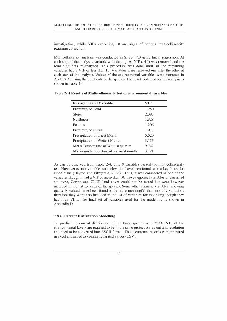
investigation, while VIFs exceeding 10 are signs of serious multicollinearity requiring correction. Multicollinearity analysis was conducted in SPSS 17.0 using linear regression. At each step of the analysis, variable with the highest VIF (>10) was removed and the remaining data re-analysed. This procedure was done until all the remaining variables had a VIF of less than 10. Variables were removed one after the other at each step of the analysis. Values of the environmental variables were extracted in ArcGIS 9.3 using the point data of the species. The result obtained for the analysis is shown in Table 2-4.
Table 2- 4 Results of Multicollinearity test of environmental variables As can be observed from Table 2-4, only 9 variables passed the multicollinearity test. However certain variables such elevation have been found to be a key factor for amphibians (Dayton and Fitzgerald, 2006) . Thus, it was considered as one of the variables though it had a VIF of more than 10. The categorical variables of classified soil type, Corine and CLUE land cover could not be tested but were however included in the list for each of the species. Some other climatic variables (showing quarterly values) have been found to be more meaningful than monthly variations therefore they were also included in the list of variables for modelling though they had high VIFs. The final set of variables used for the modelling is shown in Appendix D.
2.8.4. Current Distribution Modelling
To predict the current distribution of the three species with MAXENT, all the environmental layers are required to be in the same projection, extent and resolution and need to be converted into ASCII format. The occurrence records were prepared in excel and saved as comma separated values (CSV).
Environmental Variable VIF Proximity to Pond 1.250 Slope 2.393 Northness 1.328 Eastness 1.206 Proximity to rivers 1.977 Precipitation of driest Month 5.520 Precipitation of Wettest Month 3.156 Mean Temperature of Wettest quarter 9.742 Maximum temperature of warmest month 3.121

MODELLING THE POTENTIAL DISTRIBUTION OF THREE TYPICAL AMPHIBIANS ON CRETE, AND THEIR RESPONSE TO CLIMATE AND LAND USE CHANGE
22
Each species’ present record was randomly divided into 30 random partitions. Each partition was created by randomly selecting 75 % of the presence records for training the model and 25 % for testing. Thus P. Cretensis with a total record of 45, 34 records were set aside for training the model, whilst the remaining 11 were used for testing. However, not all the training and test data had a corresponding environmental variables in the study area, thus those records without environmental variables were subsequently removed before simulating for each species . Table 2-5 shows the partitions set aside for training, testing and the number that did not have corresponding environmental variables. Maxent was run with 3000 background points. The maximum number of iterations that allow the algorithm to get close to convergence was set to 500. The convergence threshold and regularization multiplier were all left at the default value of 0.0001 and 1 respectively. Table 2- 5 Training and Test data used in the Modelling Species Total presence
points available
Training data Test records Number of records omitted
P. viridis 89 61 19 12 P. cretensis 45 30 10 5 H. arborea 27 19 6 2 These partitions allowed for the assessment of the average behaviour of the models and also for the statistical testing of observed differences in performance of the models as proposed by Phillips et al. (2006) (see section on model evaluation for details). 30 subset models were produced for each species per each combination of environmental variables. Thus a total of 30 output maps were produced for each model. The average probability of suitability was calculated for each subset models based on the 30 output maps produced. To test whether including land cover types improved the modelling significantly; four separate categories of models were generated for each species (in a “stepwise” manner). The first category is a current distribution model of each species based on only elevation data. This is seen as the lowest level of the modelling with only elevation data and water related variables (distance to ponds and rivers). The second model is with elevation, water related variables and climate data (hereafter referred to as Model 2). The third Model generated was with elevation, water related variables and vegetation cover. Finally, a model was built with elevation, water related variables, climate and vegetation. The modelling was performed in this way to allow for the effect at each stage to be quantified in terms of the gain and AUC. Each model was run 30 times representing the 30 random subsets per species (Table 2-6 describes the components of each model).

MODELLING THE POTENTIAL DISTRIBUTION OF THREE TYPICAL AMPHIBIANS ON CRETE, AND THEIR RESPONSE TO CLIMATE AND LAND USE CHANGE
23
Table 2- 6 Models produced under current conditions MODEL VARIABLES 1 Elevation data + proximity to ponds 2 Elevation data + proximity to ponds+ climatic variables 3 Elevation data +proximity to ponds + vegetation cover 4 Elevation data+ proximity to ponds +climatic data + vegetation cover.
2.8.5. Future Prediction Modelling
To explore how future climate change may influence the potential distribution of all three species, current climate species relationship was projected onto the future estimates of climatic conditions in 2050 from the WorldClim database. A separate prediction was also done that includes potential land use in 2030. Changes in the occupancy of a species under current and future climate conditions were quantified by transforming the probability of occurrence from models into presence-absence maps. This was done by using the 10 percentile training presence threshold. Changes in suitable and unsuitable conditions were then reclassified into 4 classes as shown in Table 2-7 for each output map of future conditions. The 10 percentile threshold (described under the section on thresholds) was used to convert the probability maps into suitable and unsuitable areas. To explore the effect of both climate and land use change, three different models were produced for each species. Description of the different models is presented in Table 2-7. Table 2- 7 Models for Future distribution MODELS Variable Groups 1 Climate (2050) + Proximity to Ponds + Elevation 2 Climate (2050) + Proximity to ponds +Elevation + land cover (current)
3 Climate (2050) + Proximity to Pond + elevation + landcover(Clue Land use map 2030)
The binary map for the future prediction was given codes as follows: suitable as 2 and unsuitable as 0, current conditions were classified into suitable as 1 and unsuitable as 0. The current binary maps were then subtracted from the future maps to produce the classifications as described in Table 2-7.

MODELLING THE POTENTIAL DISTRIBUTION OF THREE TYPICAL AMPHIBIANS ON CRETE, AND THEIR RESPONSE TO CLIMATE AND LAND USE CHANGE
24
Table 2- 8 Description of current adn future classes for the change in ragne maps Class Current Suitability Future Suitability -1 Suitable Not Suitable 0 NOT suitable NOT suitable 1 Suitable Suitable 2 NOT suitable Suitable
2.8.6. Model Evaluation
The usefulness of species distribution models depends on a thorough evaluation of their performances (Liu et al., 2009). Therefore model evaluation is considered to form a very important part of model building. A model that has been subjected to a good assessment and evaluation, helps to identify the “relative strengths and weaknesses of the model and delimits the range of uses to which models can be usefully applied”. According to Pearce and Ferrier (2000), there are 2 main parts of the measurement of accuracy of distribution models; discrimination capacity and reliability. Of the two, discrimination capacity is usually seen as being more important than reliability (Ash and Shwartz, 1999). Discrimination capacity measures a models ability to distinguish between sites where the subject has been detected (presence sites) and those sites where the species is known to be absent (absence sites). Reliability describes the agreement between predicted probabilities of occurrence and the observed proportions of sites occupied by the species (Manel et al., 2001). It is a critical component in determining the quality of probabilistic predictive models. Both discrimination and reliability can be used when the modelling results is continuous, however, only discrimination can be used when the result is binary. Discrimination and reliability have both been evaluated with a number of indices. Majority of these indices tend to work on binary results or on continuous results that have been transformed into binary results using a specific threshold therefore they are referred to as Threshold-dependent.
2.8.7. Threshold Independent Evaluations of the Models
The models were evaluated using the threshold independent measure of Area Under the Curve (AUC) of the Receiver Operating Characteristics (ROC) plot (Pearce and Ferrier, 2000). The ROC is obtained by plotting sensitivity as a function of the falsely predicted positive fraction or commission error (1-specificity) for all possible thresholds of a probabilistic prediction of occurrence. The resulting area under the ROC curve provides a single measure of overall model accuracy, which is independent of a particular threshold. AUC values range from 0 to 1, with a value of 1.0 indicating the probability that when a presence site ( site where a species is recorded) and an absence site (site where species is recorded as absent) are drawn at
MODELLING THE POTENTIAL DISTRIBUTION OF THREE TYPICAL AMPHIBIANS ON CRETE, AND THEIR RESPONSE TO CLIMATE AND LAND USE CHANGE
25
random from the population, the presence site has a higher predicted value than the absence site (Elith et al., 2006; Phillips et al., 2006). The AUC value has been shown to be the only measure of accuracy that is invariable to the proportion of the data representing species presence, known as prevalence (Pearce and Ferrier, 2000; Manel et al., 2001; McPherson and Rogers, 2004). Insensitivity to prevalence is of importance when the AUC values are used to assess model accuracy for species distribution models that have been developed with presence only data. In the case of presence-only modelling, absences are replaced by pseudo-absences. Pseudo-absences are sites randomly selected across the geographical area of interest at localities where species occurrence is set to be absent (Anderson et al., 2003; Elith et al., 2006; Phillips et al., 2006). Usually a sufficiently large number of pseudo-absences are needed to provide a reasonable representation of the environmental variation exhibited by the geographical area of interest. Some authors have suggested choosing between 1000 to 10,000 points to represent pseudo-absences (Ferrier, 2002; Phillips et al., 2006). 3000 background points rather than 10,000 as has been used by many researchers for modelling and calculating the AUC due to the relatively small size of the study area. AUC values from the 30 subsets produced by each model were statistically tested to determine if they were significantly better than random as stated in objective one. The averages of the AUC’s were calculated and compared with different models. As noted by Phillips et al. (2006), the AUC calculated for data without true absences tend to be high for species with restricted ranges and low for wide ranging species, therefore AUC’s are interpreted by considering the species’ natural distribution. The 30 AUC’s produced from each model were tested for normality in SPSS. The t-statistics was then applied in determining the significance of each AUC produced against a null model (AUC=0.5).
2.8.8. Threshold Determination and Model Assessment Using Cohen’s Kappa
Most results of species distribution models are presented as probability of species presence or environmental suitability for the target species. It becomes increasingly important when assessing model performance using indices derived from confusion matrix to find a threshold that will allow for a binary map to be produced (Manel et al., 2001). There are several threshold determining approaches, however two categories are recognised in literature; subjective and objective (Liu et al., 2005). Subjective approaches such as taking 0.5 as the threshold is widely used in ecology (Manel et al., 2001; Bailey et al., 2002; Stockwell and Peterson, 2002) others have also used 0.3 (Robertson et al., 2001) and 0.05 (Cumming, 2000). However as noted by (Osborne et al., 2001)), these choices are arbitrary and lack ecological basis. Objective thresholds approaches are therefore usually chosen to maximize the agreement between observed and predicted distributions (Liu et al., 2005). Taking a subjective threshold of 0.5 may sometimes render presence/absence maps useless if

MODELLING THE POTENTIAL DISTRIBUTION OF THREE TYPICAL AMPHIBIANS ON CRETE, AND THEIR RESPONSE TO CLIMATE AND LAND USE CHANGE
26
there are uneven samples. Thresholds are required when assessing the impact of future climate change on the potential distribution of species. In such situations it is important to use thresholds that will not be too restrictive to most suitable habitats. Objective threshold such as kappa maximization approach and sum of maximum sensitivity and specificity which is equivalent to finding a point on the ROC curve whose tangent slope is equal to 1 (Cantor, 1999) have been applied by several researchers Maxent as a modelling tool also calculates several thresholds as part of the model results. These include three fixed cumulative values of 1, 5 and 10, minimum training presence, 10 percentile training presence Equal sensitivity and specificity, maximum training sensitivity plus specificity. The 10 percentile training presence was used as the threshold for converting the habitat suitability maps into binary maps in order to produce the future change maps. Kappa was calculated with ROC/AUC software (Bonn and Schroder, 2001). Also reported is the sensitivity and specificity of each model and for each species.
2.8.9. Jackknife Test of Important Variables
A Jackknife test was used to answer the questions related to the importance of the different variables. While the model was being trained, the contributions of each environmental variable were tracked at each step of the training process. As explained by Phillips et al. (2006) each time the model uses a variable the coefficient for that variable is modified, Maxent therefore assigns the increase in the gain of the model to the environmental variable that the feature depends on. A gain is similar to the goodness of fit used in generalized linear models and usually starts at 0 and increases towards an asymptote during the run of the model. The gain indicates how closely the model is concentrated around the presence samples. The average gains over the thirty (30) random subset models were calculated for each environmental variable. Two different gains were calculated; one with all other environmental variable (except the selected variable) and the second gain calculated using only the selected variable. This is to establish the effect of the variable on the performance of the model in terms of the gain. The variable that reduces the gain the most when it is excluded from the run of the model is seen as been the most important.
2.8.10. Statistical Test of Significance of Models
A statistical test was carried out to (1) test whether the average AUCs produced were better than a null or random model (with AUC of 0.5); (2) test whether the models
MODELLING THE POTENTIAL DISTRIBUTION OF THREE TYPICAL AMPHIBIANS ON CRETE, AND THEIR RESPONSE TO CLIMATE AND LAND USE CHANGE
27
were significantly different from each other. In order to decide on which test to use, a normality test was carried out in SPSS 17 to test whether the AUCs and the gains were normally distributed. Based on the normality test, a one tailed T-test was used to test for the significance of the average values against a random model. Analysis of Variance (ANOVA) was used to establish if there is any significant difference between the means of the test AUC. A pair wise comparison was then carried out to establish which two means are significantly different from each other.
2.8.11 Software and Statistical Packages
The following equipments and software were used to achieve the set objectives: a) ESRI ArcGIS 9.3 b) Arcpad 7.1 c) SPSS 17.0 d) MAXENT 3.3.3 e) Microsoft Excel and Word 2007 f) Amphibians and Reptiles Field book of Greece g) Hp IPAQ h) Endnote X2


MODELLING THE POTENTIAL DISTRIBUTION OF THREE TYPICAL AMPHIBIANS ON CRETE, AND THEIR RESPONSE TO CLIMATE AND LAND USE CHANGE
28
3.0 Results
This section presents results from the modelling and a brief discussion for each result. The section is structured in order of the four hypothesis set under section 1.4.3. Each hypothesis is tested and rejected or accepted based on significance. The section is divided into 2 main parts:1) Current Distribution Models and 2) Future distribution Modelling
3.1. Current Distribution Modelling
3.1.1. Normality Test
In order to determine which test type to employ in determining significance of the models and to compare the means, it was necessary to first check if the results obtained from the 30 random models were normally distributed. Therefore, the Shapiro-wilk test was carried out in SPSS to determine if the results obtained were normally distributed. A P-value greater than 0.05 means the data is normally distributed. Table 3-1 shows the result for the normality test with all results greater than 0.05 except for the training AUC of P.viridis which had a value of 0.035.
Table 3- 1 Results of the normality test for each species
Shapiro-Wilk Statistics
df(P.cretensis) (P. viridis) (H. arborea)
Training AUC 1 30 0.966 0.035 0.867
Test AUC 1 30 0.406 0.732 0.359
Training AUC 2 30 0.557 0.380 0.071
Test AUC 2 30 0.287 0.446 0.193
Training AUC 3 30 0.509 0.984 0.894
Test AUC 3 30 0.668 0.277 0.125
Training AUC 4 30 0.832 0.188 0.09
Test AUC 4 30 0.999 0.251 0.073 Note: 1, 2, 3 and 4 represents Model 1, Model 2, Model 3 and Model 4 respectively.
MODELLING THE POTENTIAL DISTRIBUTION OF THREE TYPICAL AMPHIBIANS ON CRETE, AND THEIR RESPONSE TO CLIMATE AND LAND USE CHANGE
29
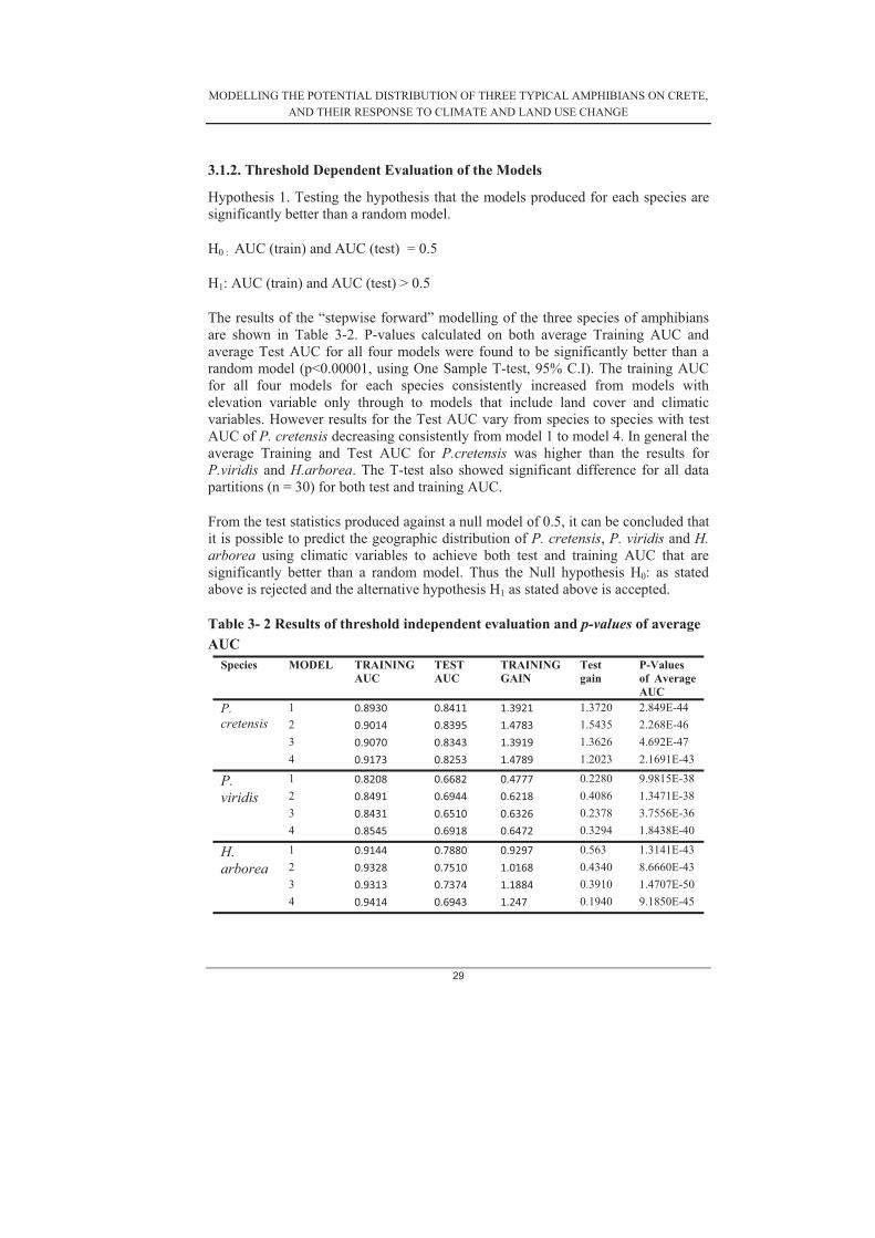
3.1.2. Threshold Dependent Evaluation of the Models
Hypothesis 1. Testing the hypothesis that the models produced for each species are significantly better than a random model.
H0 : AUC (train) and AUC (test) = 0.5
H1: AUC (train) and AUC (test) > 0.5
The results of the “stepwise forward” modelling of the three species of amphibians are shown in Table 3-2. P-values calculated on both average Training AUC and average Test AUC for all four models were found to be significantly better than a random model (p<0.00001, using One Sample T-test, 95% C.I). The training AUC for all four models for each species consistently increased from models with elevation variable only through to models that include land cover and climatic variables. However results for the Test AUC vary from species to species with test AUC of P. cretensis decreasing consistently from model 1 to model 4. In general the average Training and Test AUC for P.cretensis was higher than the results for P.viridis and H.arborea. The T-test also showed significant difference for all data partitions (n = 30) for both test and training AUC.
From the test statistics produced against a null model of 0.5, it can be concluded that it is possible to predict the geographic distribution of P. cretensis, P. viridis and H. arborea using climatic variables to achieve both test and training AUC that are significantly better than a random model. Thus the Null hypothesis H0: as stated above is rejected and the alternative hypothesis H1 as stated above is accepted.
Table 3- 2 Results of threshold independent evaluation and p-values of average AUC
Species MODEL TRAINING AUC
TESTAUC
TRAINING GAIN
Testgain
P-Values of Average AUC
P.cretensis
1 0.8930 0.8411� 1.3921 1.3720 2.849E-44 2 0.9014 0.8395 1.4783 1.5435 2.268E-46 3 0.9070 0.8343 1.3919 1.3626 4.692E-47 4 0.9173 0.8253 1.4789 1.2023 2.1691E-43
P.viridis
1 0.8208 0.6682 0.4777 0.2280 9.9815E-38 2 0.8491 0.6944 0.6218 0.4086 1.3471E-38 3 0.8431 0.6510 0.6326 0.2378 3.7556E-36 4 0.8545 0.6918 0.6472 0.3294 1.8438E-40
H.arborea
1 0.9144 0.7880 0.9297 0.563 1.3141E-43 2 0.9328 0.7510 1.0168 0.4340 8.6660E-43 3 0.9313 0.7374 1.1884 0.3910 1.4707E-50 4 0.9414 0.6943 1.247 0.1940 9.1850E-45

MODELLING THE POTENTIAL DISTRIBUTION OF THREE TYPICAL AMPHIBIANS ON CRETE, AND THEIR RESPONSE TO CLIMATE AND LAND USE CHANGE
30
3.1.3. Jackknife Test of Important Variables
The Jackknife test function in Maxent was used to answer the question regarding which environmental variable is important for the potential distribution of amphibians in Crete. Average gains with and without each variable were calculated from the 30 random distributions produced from each modelling. Freshwater, was found to be the single most important variable for the potential distribution from all the models produced for all three species. The average gain significantly decreases without freshwater whilst at the same time freshwater alone can predict the distribution with a substantial gain. Landcover happens to be the second most important variable with a clear drop in average gain when it is not in the full model. Shown in Fig. 3-1, 3-2 and 3-3 are Jackknife results for Model 4 only; however results for the other three models (shown in Appendix B) follow similar pattern with freshwater being the most important predictor variable.
Figure 3- 1 Average gains for each variable calculated from the 30 subset models produced for P. cretensis

MODELLING THE POTENTIAL DISTRIBUTION OF THREE TYPICAL AMPHIBIANS ON CRETE, AND THEIR RESPONSE TO CLIMATE AND LAND USE CHANGE
31
Figure 3- 2 Average gains for each variable calculated from the 30 subset models produced for P. viridis (Model 4)
Figure 3-3. Average gains for each variable calculated from the 30 subset models produced for H. arborea (Model 4)

MODELLING THE POTENTIAL DISTRIBUTION OF THREE TYPICAL AMPHIBIANS ON CRETE, AND THEIR RESPONSE TO CLIMATE AND LAND USE CHANGE
32
Freshwater was again found to be the most important variable for models of both H. arborea and P. viridis. However, the extent of the importance in each model differs slightly for each of the species. In a rather interesting situation land cover did not affect models for H. arborea and P. viridis as it did for P.cretensis. In the model for P. viridis, when land cover was removed from the model there was no substantial decrease in the average gain of the model. The climatic variables on the other hand did not seem to affect the models as much as expected. Climate related variables on their own achieve very little Maxent gain and when they were removed from the model did not also decrease the overall gain significantly.
(a) (b)
(c)
Figure 3-4. Distribution of average gains of a) P. cretensis (b) P. viridis and (c) H. arborea

MODELLING THE POTENTIAL DISTRIBUTION OF THREE TYPICAL AMPHIBIANS ON CRETE, AND THEIR RESPONSE TO CLIMATE AND LAND USE CHANGE
33
3.1.3. Response Curves of Predictor Variables
The response curves showing how the predictions depend on the variables are shown in Fig. 3-5, 3-6 and 3-7. For P.cretensis as elevation increases the probability of its presence decreases from about 0.85 to almost 0 at elevations above 2000m. As distance to river (water bodies) decreases the chances of finding P.cretensis also decreases. From the response curve of rivers, it is apparent that P.cretensis does not exist outside water bodies as its probability of occurrence starts decreasing beyond a distance of 0m from water. The probability of finding P. cretensis does not however depend so much on precipitation of coldest quarter as it does not achieve high probabilities. In terms of association with land cover, there is a high probability of finding P.cretensis in class 14 (water and coastal flats). It also achieves high probabilities in artificial surfaces (class 0) and Non-irrigated arable lands (class 1). This is probably due to the pools and ponds that are usually associated with such areas.
H. arborea has very high probability of occurrence at lower elevations but also has a relatively high probability at higher elevations compared with P.cretensis (probability of occurrence reduces to almost 0.1 above an elevation of ~500m). Generally, probability of presence for H.arborea also decreases with increasing distance from water sources. H. arborea seems to have high association with Corine class 14 (water sources), 6 (permanently irrigated land) and 0 (artificial surfaces). A similar pattern is found for P.viridis. However, P.viridis tends to have relatively higher probability of presence for distance to water of above 1500m.
Figure 3- 5. Response curves of P. cretensis

MODELLING THE POTENTIAL DISTRIBUTION OF THREE TYPICAL AMPHIBIANS ON CRETE, AND THEIR RESPONSE TO CLIMATE AND LAND USE CHANGE
34
Figure 3- 6. Response curves of H. arborea
Figure 3- 7. Response curves of P. viridis

MODELLING THE POTENTIAL DISTRIBUTION OF THREE TYPICAL AMPHIBIANS ON CRETE, AND THEIR RESPONSE TO CLIMATE AND LAND USE CHANGE
35
3.1.4. Comparison of the Means of the Models
Hypothesis Two
H0: AUC1 = AUC2; where AUC1 = Model with climatic variables and AUC2= Model that include landcover cover.
H 1 = AUC1 � AUC2
Table 3- 3 Results of the pair-wise comparison of the four models developed per species (p-values shown)
Species PAIR WISE COMPARISON OF MODELS 1,2 1,3 1,4 2,3 2,4 3,4 P.cretensis
AUCtr 0.011 <0.0001 <0.0001 0.0613 3.104E-5
0.00441
AUCts 0.897 0.596 0.2689 0.655 0.2824 0.50307
H. arborea
AUCt 3.248E-5 1.8365E-6 1.934E-9 0.6577 0.0367 0.0018
AUCts 0.2406 0.240677 2.9692E-4 1.00 0.01028 0.0102 P.viridis
AUCt 2.371E-7 1.00940E-4 5.4039E-10
0.2650 0.23803 0.0279
AUCts 0.20805 0.42906 0.2153 0.0433 0.8862 0.0390 Note: AUCtr = training AUC and AUCts = test AUC
Analysis of Variance (ANOVA) was done to test if there is difference in the means of both the test and training AUC produced for each species under the four models (results shown in Appendix C). The ANOVA results show that there is no significant difference in the means of AUC of all four models for P. cretensis. However, results for P.viridis and H.arborea show that at least two of the models are significantly different in terms of the test AUC. To further test which two means are significantly different, a pair wise comparison of the models was done. The training AUC for all pairs of means of the models produced for P. cretensis were significantly different from each other (except for models 2 and 3). However, there is no significant difference (p < 0.05) between models 4 (elevation plus vegetation and climate variables) and all other models produced for P.cretensis. Models 2 and 3 again did not show any significance for H. arborea and P. viridis in terms of the training AUC.
Contrary to the training AUC, a comparison of the means of the test AUC did not show any significant difference for all model combinations with the exception of models 3 and 4 for P.viridis and 2 and 4 for H.arborea (P < 0.05). The performance of each model is based on how well the model is able to predict the test data (Fielding and Bell, 1997). Therefore based on the pair wise comparison of the means

MODELLING THE POTENTIAL DISTRIBUTION OF THREE TYPICAL AMPHIBIANS ON CRETE, AND THEIR RESPONSE TO CLIMATE AND LAND USE CHANGE
36
of the models, it can be concluded that all four models have the same predictive power in terms of the test AUC for P. cretensis (the test means were not significantly different from each other). Thus the distribution of P. cretensis for instance, can be adequately predicted with just elevation predictors and proximity to ponds. Logically the best model for P. cretensis will then be the one that is able to adequately predict the potential distribution with as few predictor variables as possible and achieve a test AUC that is not significantly different from a model that make use of the full range of available predictor variables (model 4).
The overall minimum, maximum and standard deviation of models with climatic data and models with both climatic and land cover are shown in Table 3-4. The standard deviations of models with climatic data were higher than models with both climatic and land cover variables for all three species.
Table 3- 4 Statistical summary of the AUC from the ROC curve displaying the standard deviation (SD) the minimum (min) and the maximum (max) for each species under models with and without land cover.
Elevation + climatic data
Elevation + climatic + vegetation
Min Max SD Min Max SD P.cretensis 0.7316 0.9084 0.059507 0.6956 0.9498 0.06227 H.arborea 0.5739 0.8991 0.092947 0.4175 0.8603 0.11737 P.viridis 0.4898 0.8266 0.07812 0.5587 0.7849 0.07860
Gains produced from Maxent modelling have also been used in determining the best performing model (Yost et al., 2008). Gains describe how well the model fits to the training or test dataset available. The average gains for all four models for all three species show that, models with elevation and climate only and those with both climate and land cover achieved the highest average training gains (Fig.3-4 shows the distribution of the gains in terms of means). A two tailed independent t-test shows that the means are significantly different (t = 6.265, p<0.00001 95% CI).
3.1.6. Models without Proximity to Ponds
Fig. 11 shows the average test gain and training gains when proximity to freshwater ponds are omitted from the four modelling. For all four models, average test AUC and average training gains decreased for all three species when proximity to freshwater are omitted from the model. Proximity to freshwater bodies is therefore an important predictor variable for all three species of amphibians in Crete.

MODELLING THE POTENTIAL DISTRIBUTION OF THREE TYPICAL AMPHIBIANS ON CRETE, AND THEIR RESPONSE TO CLIMATE AND LAND USE CHANGE
37
(a) H.arborea
(b) P.viridis
c) P.cretensis

MODELLING THE POTENTIAL DISTRIBUTION OF THREE TYPICAL AMPHIBIANS ON CRETE, AND THEIR RESPONSE TO CLIMATE AND LAND USE CHANGE
38
Figure 3- 8. shows the average test AUC and gains of models with and without proximity to freshwater bodies for (a) H. arborea (b) P. viridis (c) P. cretensis
3.1.7. Binomial Test Statistics
Table 3- 5 Average test omission rate and average fractional predicted area calculated for two threshold levels (average over 30 subsets) 10 percentile training
threshold Maximum sensitivity plus
specificity
Species name
Model Fractional Predicted Area
Test omission rate
Fractional Predicted Area
Test omission rate
Pelophylax cretensis
1 0.3467 0.1744 0.1458 0.3333�2 0.3504 0.1538 0.1086 0.4231�3 0.2921 0.1205 0.1501 0.3744�4 0.3076 0.0195 0.1261 0.4205�
Hylaarborea
1 0.2687 0.1867 0.2559 0.1467�2 0.2134 0.1207 0.1795 0.44�3 0.2597 0.1067 0.1354 0.533�4 0.2156 0.0513 0.1286 0.6�
1 0.4905 0.2878 0.2868 0.4500�P. viridis 2 0.4556 0.2744 0.2021 0.5417� 3 0.4588 0.1472 0.3858 0.2750� 4 0.4488 0.0778 0.3174 0.2972�
Two indicators were used under the binomial test statistics to examine model performance: the fraction of predicted area and the extrinsic omission rate. These were calculated using the 25% of test data set aside during the modelling process in Maxent. Two levels of threshold were also compared. The results for the two levels of thresholds are shown in Table 3-5. All omission test rates calculated at the 10 percentile training presence threshold were lower than those calculated at the maximum sensitivity plus specificity threshold. The fractional predicted area shows the fraction of all the pixels that are predicted suitable for the species (Phillips et al., 2006). The test omission rates for model 4 were consistently less than models 2, 3, and 1. This suggests that a small fraction of the test locations fell into pixels not predicted as suitable for the species. Fractional predicted areas for P.viridis were higher than for P. cretensis and H. Arborea (reasons for these are discussed further in Chapter 4). A two tailed Wilcoxon-signed ranked test on the medians between Model 2 and 4 did not show any significant difference in median of fractional

MODELLING THE POTENTIAL DISTRIBUTION OF THREE TYPICAL AMPHIBIANS ON CRETE, AND THEIR RESPONSE TO CLIMATE AND LAND USE CHANGE
39
predicted (p= 0.1284 and 0.2421 at the 10 percentile training threshold and equal sensitivity and specificity threshold respectively).
3.1.8. Kappa Statistics Results
Table 3- 6 Average Kappa, sensitivity and specificity calculated on the 25% test dataset for model with and without vegetation
Model Species Kappa
Sensitivity specificity
Climate P.cretensis 0.669 76.92% 79.59% H. arborea 0.305 50% 50% P. viridis 0.814 75% 75.55% Climate + vegetation
P. Cretensis 0.823 75% 73.47%
H. arborea 0.405 50% 50% P. viridis 0.808 58.33% 85.71%
Kappa was calculated for models produced with and without land cover. The results show that kappa values for the two models are significantly different from each other, kappa values for the climate model for all species were significantly lower than for models with vegetation cover (one tailed t- test p=0.0312 (P.cretensis), p < 0.01 (H. Arborea) and p= 0.0412 (P. viridis) all at 95% CI). The climate and vegetation models for all three species predict species distributions that have good agreement with observed species points. The inclusion of land cover seems to increase the overall agreement of the observed points with the predicted.
In terms of sensitivity (true positive rates) and specificity (true negative rates), the climate model was again more superior to the model with vegetation cover. P.cretensis in both models achieved almost similar sensitivity but still low in the model with vegetation cover. H. Arborea and P. viridis showed similar trend with model for P. viridis being able to predict absences (specificity = 85.71%) better than presences (58.33%).
3.1.9. Current Potential Distribution Models
Fig 3-9 and Fig 3-10 show maps of potential distribution of the two species with and without vegetation cover. The maps are showing averages of the 30 maps produced from the 30 random partitions of each species occurrence records. The maps clearly depict areas with ponds as having very high potential habitat suitability values. There is however no observable difference between models produced with and without vegetation cover. P. cretensis seems to avoid higher altitudes with high suitability areas found in lower elevations along the coast whilst P.viridis and H.arborea have wide distribution across Crete. Even though there are some freshwater ponds recorded up on higher altitudes, maps for P.cretensis show these areas as having very low suitability because P.cretensis is generally found at elevations of 100m and below.
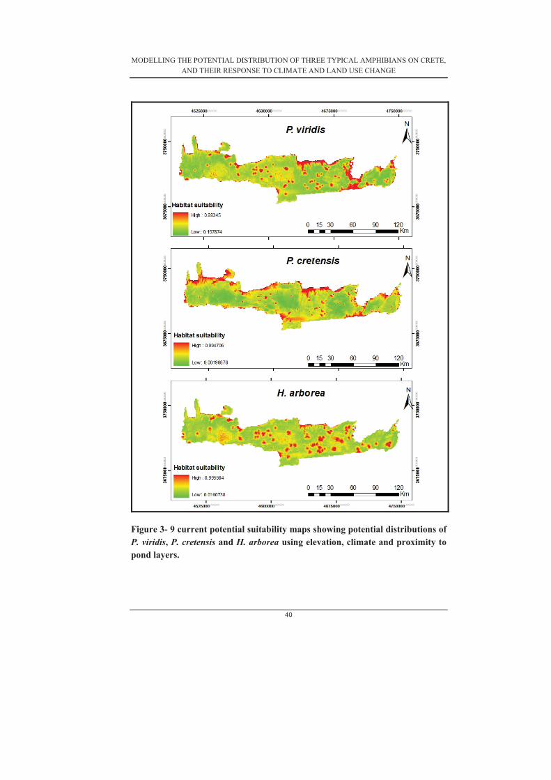
MODELLING THE POTENTIAL DISTRIBUTION OF THREE TYPICAL AMPHIBIANS ON CRETE, AND THEIR RESPONSE TO CLIMATE AND LAND USE CHANGE
40
Figure 3- 9 current potential suitability maps showing potential distributions of P. viridis, P. cretensis and H. arborea using elevation, climate and proximity to pond layers.
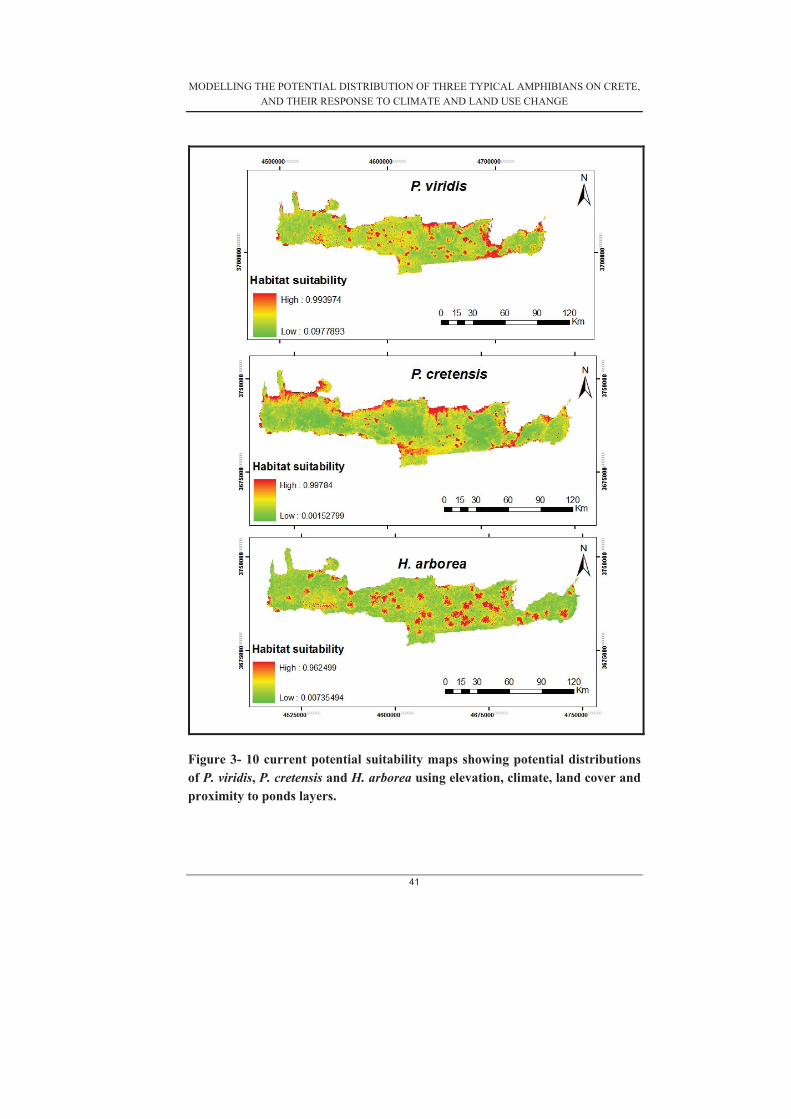
MODELLING THE POTENTIAL DISTRIBUTION OF THREE TYPICAL AMPHIBIANS ON CRETE, AND THEIR RESPONSE TO CLIMATE AND LAND USE CHANGE
41
Figure 3- 10 current potential suitability maps showing potential distributions of P. viridis, P. cretensis and H. arborea using elevation, climate, land cover and proximity to ponds layers.

MODELLING THE POTENTIAL DISTRIBUTION OF THREE TYPICAL AMPHIBIANS ON CRETE, AND THEIR RESPONSE TO CLIMATE AND LAND USE CHANGE
42
3.2 Future Distribution Maps
Visual observations indicate that under the first assumption (Model 1) current potential distribution for P.viridis did not change much in the future. However, there seems to be an increase in the potential suitability areas and a slight loss of potential suitability areas especially up on the higher elevations. Model 2 for P.viridis also shows a substantial gain in range than actually loss. The prediction for the easternmost part of Crete is almost similar in all three models. However, substantial amount of current suitability areas will be lost in Model 2 than in Model 3 and 1. A gain in range can be observed in the higher altitudes which suggest a shift toward higher altitudes for P. viridis.
H. arborea unlike P.viridis did not gain any range in the future under Model 1. Under the second Model, a much wider area is predicted as unsuitable in the future though they are predicted as currently suitable. Small patches of areas have been predicted as suitable in the future though they are not suitable under current conditions. The model for H. arborea shows similar change as in the second assumption. Fig. 3-11 shows number of grid cells that will be loss or gain.
P. cretensis deviates markedly from the two other species in the future potential distribution. Model 1 shows that most of the areas currently predicted as suitable will not be suitable in the future. The ponds can clearly be seen to be suitable in the future in addition to a very small area that is currently not suitable but predicted to be suitable in the future.
Fig 3-11. Potential number of grid cells that will be loss or gain based on the future predictions
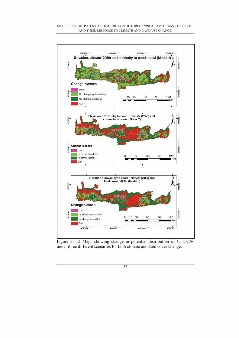
MODELLING THE POTENTIAL DISTRIBUTION OF THREE TYPICAL AMPHIBIANS ON CRETE, AND THEIR RESPONSE TO CLIMATE AND LAND USE CHANGE
43
Figure 3- 12 Maps showing change in potential distribution of P. viridis under three different scenarios for both climate and land cover change.

MODELLING THE POTENTIAL DISTRIBUTION OF THREE TYPICAL AMPHIBIANS ON CRETE, AND THEIR RESPONSE TO CLIMATE AND LAND USE CHANGE
44
Figure 3- 113 Maps showing the change in potential distribution of H. arborea under the three different scenarios for both climate and land use change

MODELLING THE POTENTIAL DISTRIBUTION OF THREE TYPICAL AMPHIBIANS ON CRETE, AND THEIR RESPONSE TO CLIMATE AND LAND USE CHANGE
45
Figure 3- 124 Maps showing change in potential distribution of P. cretensisunder the three different scenarios for climate and land use change.

MODELLING THE POTENTIAL DISTRIBUTION OF THREE TYPICAL AMPHIBIANS ON CRETE, AND THEIR RESPONSE TO CLIMATE AND LAND USE CHANGE
46
4.0 Discussion
This section discusses the results relating it to quality of data used in the modelling; ecological significance of the output of the modelling and how the results could be improved in future work. Current potential distribution of the species and the influence of ponds in the distributive models are discussed. Predictions for the future are also considered and related to the broader frame of how each species may behave giving what we know of their ecology. This is then related to the uncertainties that can result from change in land use or interaction with other species.
4.1 Inference from model evaluation
4.1.1. Threshold Independent Evaluation
The current potential distribution models for P.cretensis seem to agree quite well with the sample points. All four models produced for P. cretensis consistently predicted potential distribution better than random. The area under the ROC curve for all partitions was consistently higher than for the other two species. All four models achieved a relatively high test AUC (mean test AUC > 0.8253, average standard errors for all four models less than 0.057 at 95% CI). What is most interesting is the fact that a reasonably high AUC (from Table 3-2. Model 1 average AUC = 0.8411±0.0194) was achieved for a model that included elevation variables and freshwater layer. However, this was not significantly different from models with vegetation and climatic variables included. In terms of significance the results show better than random prediction for all models (one tailed t-test p < 0.00001). According to Phillips et al. (2006), a perfect model should contain a set of environmental variables that sufficiently describes all the parameters of the species’ fundamental niche relevant to its distribution at the spatial scale of the model. Therefore even though the model with elevation variables and freshwater layer did not significantly differ from a model with climatic and vegetation variables in terms of performance, it is difficult to say that the output of such a model captures the full range of habitat conditions available for P. cretensis. The main aim of modelling in a stepwise manner as done with the range of variables available for this modelling was to determine how the test AUCs change with the addition of each set of variables. In this way the impact of both climatic and vegetation cover could be estimated ( as per objective 2 which seeks to determine if vegetation or climatic variables have more impact in terms of performance on the distribution of the species).
The average test AUC achieved for P.viridis and H. arborea were generally lower than for P. cretensis. Average means were especially lower for P. viridis and this can be explained by the fact that ROC/AUC is usually affected by the type of species under consideration and whether the species is a wide or narrow ranging species, and for presence only modelling the maximum achievable AUC is less than 1 (Phillips et al., 2006). It must be emphasized here that P.viridis is a wide ranging species which occupy wide geographic areas and lives under wide environmental space than both P. cretensis and H. arborea. Therefore results obtained here are in

MODELLING THE POTENTIAL DISTRIBUTION OF THREE TYPICAL AMPHIBIANS ON CRETE, AND THEIR RESPONSE TO CLIMATE AND LAND USE CHANGE
47
agreement with other findings (Hernandez et al., 2006). P. viridis is a very robust amphibian and is highly tolerant to very dry conditions than most other amphibian species, including P. cretensis and H. arborea (Kuzmin, 1999).
P.cretensis is purely an aquatic species and belongs to the order Ranidae which are said to be true frogs. Records from the study area suggest they have been observed at a mean height of 125m above sea level with maximum observed height at around 305m compared with Hyla arborea and P. viridis at mean and maximum heights of 289m, 1520m and 417m, 1780m respectively. The potential distribution maps of P. cretensis produced are therefore concentrated almost entirely on the lowland of Crete with small patches scattered in areas where ponds and wetlands have been observed. A comparison of the binary distribution maps produced for each species with maps found on Amphibiaweb, shows high similarity with the predicted maps. Therefore all three species were reasonably modelled with P.viridis and H.arborea showing widespread distribution within Crete and P.cretensis clearly absent from the higher altitudes and seem to have high potential distribution in the low grounds.
The AUC results should be interpreted with caution because of the behaviour of the ROC/AUC when applied to presence only models (Anderson et al., 2003). As can be observed from the four models produced for each species (Table 3.6), a higher AUC was achieved for model that includes only elevation variables for P. cretensis and H. arborea. In realistic terms, such a model does not contain all the range of variables that will represent the species niche. The model says nothing about the influence of climate neither does it say something about the effect of land use or land cover on the potential distribution. As noted by (Lobo et al., 2008), the AUC is a discrimination index that represents the likelihood that a presence will have a higher predicted value than an absence regardless of the goodness-of-fit of the predictions. It is therefore possible that a poorly fitted model that overestimate or underestimate all the predictions will have a good discrimination power and vice versa in cases where probabilities for presences are moderately higher than those for absences. Due to these uncertainties or draw backs with the use of AUC, the models were also evaluated by comparing the average training gains obtained from Maxent. Phillips etal.(2006) described the gain obtained from Maxent models as similar to the goodness of fit that is usually used in generalized additive and generalized linear models. Therefore the gains from each model were compared to further validate the results from the AUC. According to Yost et al. (2006), if the main objective is to identify the most powerful predictor variables, then it is prudent to consider very small improvement in average training gains for each model. Result obtained based on the gains (Table 3-2 and Appendix C), were used to determine the power of climatic variables and vegetation cover on the models. In all cases, the average training gain over the 30 subsets shows a significant improvement over the model with only elevation variables

MODELLING THE POTENTIAL DISTRIBUTION OF THREE TYPICAL AMPHIBIANS ON CRETE, AND THEIR RESPONSE TO CLIMATE AND LAND USE CHANGE
48
4.1.2. Threshold Dependent Evaluation
The choice of thresholds has a significant impact on the results expected from species distribution models especially if the results are used to identify change in potential distribution under climate change. The threshold adopted will also have profound effect on the accuracy of the models based on the extrinsic test omission rate and fractional predicted area as calculated by Maxent. A low omission rate is necessary but not a sufficient condition for good model (Anderson et al., 2003). Thresholds are generally chosen with species ecology and reality within the study area as main considerations (Osborne et al., 2001). The Optimal threshold for the application in binary maps such as those used in determining range shift is still unresolved within the predictive species distribution circles (Anderson et al., 2003; Liu et al., 2005; Phillips et al., 2006).
The 10 percentile training threshold has been used by several authors to investigate range shift under climate change (Berry et al., 2002; Araujo et al., 2006; Beaumontet al., 2008). It has been applied especially in species with low dispersal ability and has been considered as a more conservative threshold because it tends not to overestimate the potential distribution area (Rodder et al., 2009). The 10 percentile training threshold represents “ten percent of each species records with the lowest prediction values will fall into the absence regions, and the presence regions will be made up of the other 90% of the distribution records” (Fielding and Bell, 1997; Antoine Guisan, 2000). Test omission rates for P. cretensis for all four models produced was less than 18% indicating that 82% of the test records will be correctly predicted by the model as presences under the 10% training threshold. However, test omission rate under the Maximum sensitivity plus specificity were much high for all four models.
H.arborea obtained a test omission rate almost similar to P.cretensis but with much smaller predicted area under both thresholds being considered. H.arborea is quite selective in its habitat especially in mountainous areas like the Island of Crete where it has been found to live mostly in forests and in more or less wet landscapes (Stocket al., 2008).
Results of Fractional Predicted Area are quite different for all three species with P.viridis having much higher predicted areas than for P.cretensis and H.arborea. P.viridis being a wide ranging species, it is reasonable to see a higher fraction of the area predicted as suitable. Kappa values were also significantly lower for the climate only model compared with the model that includes land cover.
4.2. Environmental Predictor Variables
4.2.1 Effect of Proximity to Ponds
Amphibians are highly adapted to water and are greatly influenced by the availability of water. It is therefore not surprising that “proximity to ponds” was found to be the most important predictor variable for all three species. Of the three

MODELLING THE POTENTIAL DISTRIBUTION OF THREE TYPICAL AMPHIBIANS ON CRETE, AND THEIR RESPONSE TO CLIMATE AND LAND USE CHANGE
49
species considered in this study, P.cretensis is the only true aquatic species which spends almost the entire time in water. Results from the Jackknife test suggest that for the climate models, the average contribution of “freshwater layer” was more than 60% to the distribution. In terms of gains, freshwater turned out to be the single most important variable for the predictive models for all three species. Figure 3-1 shows gains achieved by the climate model built with only freshwater and the total average training gain achieved with all variables included. Clearly P.cretensis achieved the highest training gain followed by H.arborea and P.viridis. Proximity to freshwater alone achieves a training gain that is more than half the gain achieved with all predictor variables for P.cretensis and H.arborea and about a quarter for P.viridis. Though, freshwater layer is still the most important predictor variable for P.viridis, its relative gain is smaller than with the other two species. This finding is quite remarkable bearing in mind the fact that P.viridis can be found both in very dry places and are most of the time found very far away from water sources. Thus they do not depend on water as much as P.cretensis and H.arborea. The results are consistent with what was found by Dayton and Fitzgerald (2006), who modelled the distribution of desert amphibians in Big Bend National Park in the USA. They concluded in their study that Bufo debilis (same group with P.viridis) are less dependent on water and only occasionally visit ponds to rehydrate and breed.
4.2.2. Importance of Landcover
It was hypothesized that the inclusion of land cover (CORINE) in the modelling could improve the model performance and result in better estimation of the potential distribution of the three species. However, results obtained indicate that landcover did not improve the model results significantly for P. cretensis. The test AUC achieved with model that included land cover was higher than models without land cover for P. viridis (Table 3-2). However, it was not significantly different from a model that did not include land cover. Results also shows that test AUC were significantly lower for Model 1(climate and land cover) than all other models for H.arborea .Visual observations did not also reveal any difference between models with only climatic variables and models that include land cover. Although results obtained did not show any significant improvement in the performance of the model with land cover, a look at the response curves produced from Maxent helps to establish the relative importance of each of the classes contained in the CORINE land cover. For instance, there was high probability of presence for CORINE class 14 (water courses) for all three species. It must be emphasize here that only few of the occurrence records were found in water courses contained in CORINE yet these areas were predicted as areas with high probability of presence for all three species.

MODELLING THE POTENTIAL DISTRIBUTION OF THREE TYPICAL AMPHIBIANS ON CRETE, AND THEIR RESPONSE TO CLIMATE AND LAND USE CHANGE
50
4.2.3. Response to Climatic Variables
Distribution of both plants and animals are broadly influenced by their physiological tolerance to climatic factors (Woodward, 1992). This is particularly true for species at various spatial scales. However, it has widely been recognised that the influence of climate is best expressed at large spatial scales(Rahbek and Graves, 2001; Thuiller et al., 2004). The spatial scale at which this study was conducted needs to be discussed. Crete is a relatively small Island and the modelling results indicate that at this small scale, climate related variables did not have significant impact on the distribution of all three species of amphibians under consideration. Elevation and proximity to water bodies make up the five most important predictor variables (Fig.3-1, 3-2 and 3-3). Climate variables do not contribute significantly in terms of the overall gains achieved by the models. From the Jackknife test it can be observe that the climate variables when used alone achieve relatively high gains, however when they are taken out of the model they do not decrease gain significantly. This suggests that probably the information contained in the climatic variables is also contained in other variables or is not useful for the distribution. Therefore it can be concluded that in Crete, the important variables defining distribution of the three amphibians are biophysical and distance to water related variables. Climate could have an effect on the distribution, but this will be an indirect effect on the occurrence and amount of water bodies available on the Island. Being a typical Mediterranean climate with projected increase in temperature and decrease in overall rainfall (IPCC 2007), the possibility of decreasing ponds availability cannot be ignored. The fact that climate related variables are not as important as land cover and proximity to ponds concurs with known factors that are causing amphibian decline in Europe; habitat loss, fragmentation and degradation (Gomez-Rodriguez et al., 2009). In Crete just like in most other places of the world amphibians are typically reliant upon artificial aquatic habitats, such as drinking trough, dug out ponds within agricultural lands etc. for breeding habitats.
4.2.4. Future Distribution
The projected distribution of P. cretensis, P. viridis and H. arborea under 2050 climate scenarios showed considerable effects on the distribution of the three species. The results show that there could be some expansion and contraction under the different assumptions made for the 2050 conditions. The future potential

MODELLING THE POTENTIAL DISTRIBUTION OF THREE TYPICAL AMPHIBIANS ON CRETE, AND THEIR RESPONSE TO CLIMATE AND LAND USE CHANGE
51
distributions of the three species were predicted under three assumptions for 2050 conditions. In all situations there will be some range reduction and range increase especially for P. cretensis and P. viridis whilst H.arborea obtained mixed results under the assumptions made. However results obtained does not follow any clear pattern. For instance, it is known that species will move poleward and on higher altitudes with changes in climate (Carey and Alexander, 2003; Araujo et al., 2006; Girardello et al., 2009). Though the clear pole ward shifts in range could not be established for the distribution, the results suggest that most of the range gain occurred in the higher altitude and thus confirm findings from other studies which suggest an altitudinal movement of species under climate change. P. viridis is a wide ranging species (generalist), and is expected to expand in range under climate change. This stood out quite clearly under all three scenarios of future change in climate and habitat. Unlike P. viridis, P. cretensis and H. arborea being more specific in their habitat preference tend to contract under the various assumptions of the future change.
4.2.5. Uncertainties in the Predictions
Although results obtained in this study suggest that climate change may have some effects on amphibian distribution in Crete, there are some sources of uncertainty that need to be considered in order to verify the accuracy of any conclusions generated by this study. Species distribution models in general are subject to a well documented range of assumptions as has been noted by several researchers (Davieset al., 1998; Thuiller, 2004; Araújo et al., 2005; Hijmans and Graham, 2006). Results obtained from future distribution models cannot be viewed as precise forecasts because of the uncertainties present in climate change scenarios and in the modelling techniques used. Future predictions do not only rely on the bioclimatic method used in modelling but also the ability of the future climate scenario to accurately show the effect of CO2 on future climate. There are several climate change scenarios available under the IPCC report (2007). The choice of a particular scenario could greatly influence the results obtained for future distribution of species. The results obtained here is thus related to only scenario under the HADCM3 models for the A2 storyline. The A2 scenario was particularly chosen because it has been thought to be more safe for species diversity than B1 and B2 scenarios (Thuiller, 2004). Thus the A2 scenario represents a more environmentally
MODELLING THE POTENTIAL DISTRIBUTION OF THREE TYPICAL AMPHIBIANS ON CRETE, AND THEIR RESPONSE TO CLIMATE AND LAND USE CHANGE
52
minded world, because on average there are lower emissions of CO2 under A2 than B1 and B2 storyline. The modelling results for both current and future climatic conditions did not take into consideration some key factors that influence distribution of species such as biotic interaction, dispersal etc. Climate change is not an abrupt process that suddenly occurs and causes species range to expand or reduce, but rather a process that tends to be gradual in nature. Species have over the years developed adaptive mechanisms that will enable them to adapt to changing conditions. These adaptive mechanisms include the ability to disperse to favourable areas as current conditions become unsuitable (this is particularly true for generalist species like P.viridis who are able to exploit favourable conditions within a fragmented landscape) and the ability to adjust to these changes. P. cretensis being a specialist species for instance is expected to be severely affected if rainfall decreases and temperature increases such that ponds and wetlands begin to dry up. However this is not clearly captured in the future distribution models leading to more uncertainties. Increasing global warming means farmers and landowners will rely more on dug out holes for water, this might open new breeding grounds for amphibians such as P. viridis and H. arborea. Thus in the future though conditions might move more towards un-favourability for amphibians, they may also take advantage of other currently unsuitable patches within their range. The CLUE land use map used in the future prediction is potential land use for 2030. This was the closest land use change map that could be obtained. However, the change in land use may not reflect the real changes in the future as the map is based on assumptions made for the future. This results in the introduction of further uncertainties in the future predictions.


MODELLING THE POTENTIAL DISTRIBUTION OF THREE TYPICAL AMPHIBIANS ON CRETE, AND THEIR RESPONSE TO CLIMATE AND LAND USE CHANGE
53
5.0. Conclusion and Recommendations
5.1. Conclusion
Increasing decline of amphibian species in the world has led to an overwhelming call for amphibians to be used for monitoring environmental quality and change (Hopkins, 2007). Several studies have shown the relevance of climate and habitat change effect on the distribution and the decline of amphibian populations worldwide (Carey and Alexander, 2003; Johnson et al., 2007; Girardello et al., 2009). The current study assessed the potential of predicting the distribution of three amphibian species (in terms of distribution) in Crete with both climatic and land cover. Results show that it is possible to predict the distribution with very high accuracy in terms of both Cohen kappa and AUC. The modelling results will go a long way to help in identifying suitable areas for the three species of amphibians as well as relating the suitability areas with other amphibian species in Crete. With increasing habitat fragmentation and continuous drying up of wetlands due to increasing climate change, it is very necessary to put in place policies that will help in the protection and conservation of amphibians in Crete. Potential distribution maps under current conditions agree very well with what has been published in literature (example www.amphibiaweb.com and Efstrastios et al.(2008)). P.cretensis was well predicted under the current conditions and was found to be highly associated with low altitudes along the coast and strongly avoided the high altitudes. H. arborea and P. viridis were also found to be widespread in Crete. Projected future distributions of the three species show that there will be both expansion and contraction of suitability areas for all three species under the 2050 climatic conditions and land use change projections for 2030. However, extent of change varies for each species and does not follow the northward movement of species under climate change as observed by other researchers (Thuiller, 2004; Pearson et al., 2007; Girardello et al., 2009). This finding is attributed to the small extent of Crete and the unavailability of the full range of environmental extremes needed to elucidate that clear climatic effect on amphibians. Despite several uncertainties, the results provide an idea of how the potential effect of climate and land use may affect amphibians in Crete. Specific results based on the set objectives are: The potential distribution of P. cretensis, P. viridis and H. arborea were adequately modelled with relatively high accuracy. The test AUC achieved for each species were significantly better than a random model. Maps of the models agree quite well

MODELLING THE POTENTIAL DISTRIBUTION OF THREE TYPICAL AMPHIBIANS ON CRETE, AND THEIR RESPONSE TO CLIMATE AND LAND USE CHANGE
54
with observed distribution points as well as with published distributions of amphibians in Crete The modelling results suggest that the distribution of P. cretensis and H. arborea could easily be predicted using only elevation parameters and proximity to water with a test AUC that is not significantly different from a model that contains all predictor variables. Whilst the combination of climate and land cover improved the test AUC for P. viridis significantly from all other models in terms of test AUC, land cover did not significantly improve models for P. cretensis. Proximity to freshwater bodies was found to be the most important predictor variables for all three species. Land cover was the second most important predictor variable in terms of training gain. The climate related variables did not decrease the gains much when they were excluded in the models. Suggesting that at the spatial scale of Crete, climate is probably not very important in determining the distribution of the three species. Future predictions did not show any clear pattern in relation to loss or gain in range for all three species. Species are adapted to specific bioclimatic conditions which tend to shift polewards as climate change. However, the modelling results did not show that pole ward movement suggesting that the study area might be too small for such poleward movement to be noticed. Regardless of this lack of poleward pattern, the results shows there will be gain and loss of habitat for all three species.
5.2. Recommendations
1. At the spatial extent of Crete, climate related variables were not found to
have influence on the distribution of the species. Therefore the general pattern of climate change could not be observed on the Island. Modelling at a bigger spatial extent (for the whole of Greece for example or the whole of the Mediterranean) can give a complete view of the future change in climate. Climate models tend to provide realistic representations at large-scale without good descriptions at local level (Benstad, 2004)

MODELLING THE POTENTIAL DISTRIBUTION OF THREE TYPICAL AMPHIBIANS ON CRETE, AND THEIR RESPONSE TO CLIMATE AND LAND USE CHANGE
55
2. The projections onto future climate models did not take into consideration dispersal ability of each species. Therefore future research may include a layer that describes cost surfaces representing the ability of species to move from one point to the other. This will require a much detailed field work to establish which ponds or wetlands are colonize by each of the species in order to create the friction or cost surfaces.
3. Due to time constraints the projection into future climate is based on only
one scenario. However as noted by Beaumont et al. (2008) future distribution models based on only one scenario may sample an unknown fraction of the uncertainty, therefore projections under different scenarios will help compare and quantify uncertainties. Future work on amphibians in Crete can therefore consider several future climate change scenarios and models in order to compare and quantify differences.

MODELLING THE POTENTIAL DISTRIBUTION OF THREE TYPICAL AMPHIBIANS ON CRETE, AND THEIR RESPONSE TO CLIMATE AND LAND USE CHANGE
56
REFERENCE Amphibiaweb. Available online at: http://amphibiaweb.org/ [Accessed on 12 December 2010] Anderson, P.R., Lew, D., Peterson, A.T., 2003. Evaluating predictive models of species' distributions: criteria for selecting optimal models. Ecological modelling 162, 211-232.
Antoine Guisan, N.E.Z., 2000. Predictive habitat distribution models in ecology. Ecological Modelling 135, 147-186.
Araújo, M., Pearson, G.R., Thuiller, W., 2005. Validation of species-climate impact models under climate change. Global Change Biology 11, 1504-1513.
Araujo, M.B., Thuiller, W., Pearson, G.R., 2006. Climate warming and the decline of amphibians and reptiles in Europe. 2006 33, 1712-1728.
Ash, A., Shwartz, M., 1999. R2: a useful measure of model performance when predicting a dichotomous outcome. . Statistic in Medicine 18, 375-384.
Austin, M., 2007. Species distribution models and ecological theory: A critical assessment and some possible new approaches. Ecological Modellin 200, 1-19.
Austin, M.P., Smith, T.M., 1989. A new model for the continuum concept. Vegetatio 83, 35-47.
Bailey, S.A., Haines-Young, R.H., Watkins, C., 2002. Species presence in fragmented landscapes: modelling of species requirements at the national level. Biological Conservation 108, 307-316.
Beaumont, L., Hughes, L., Pitman, A., 2008. Why is the choice of future climate scenarios for species distribution modelling important? Ecology letters 11, 1135-1146.
Beebee, T.J.C., Griffiths, R.A., 2005. The amphibian decline crisis: A watershed for conservation biology? Biological Conservation 125, 271-285.
Benstad, R., 2004. Empirical-statistical downscaling in climate modelling. . Ecosystem 85, 517-442.
Bererli, P., Hotz, H., Tunner, H.G., Heppich, S., Uzzell, T., 1994. Two new water frog species from the Aegean islands Crete and Karpathos. Notulae Naturae, Academy of Naturral Sciences of Philadelphia 470, 1-9.

MODELLING THE POTENTIAL DISTRIBUTION OF THREE TYPICAL AMPHIBIANS ON CRETE, AND THEIR RESPONSE TO CLIMATE AND LAND USE CHANGE
57
Berry, P.M., Dawson, T.P., Harrison, P.A., Pearson, G.R., 2002. Modelling potential impacts of climate change on the bioclimatic envelope of species in Britain and Ireland. Global Ecology and Biogeography 11, 453-462.
Bonn, A., Schroder, B., 2001. Habiat models and their transfer for single and multi species groups: a case study of carabids in an alluvial forest. Ecography 24, 483-496.
Brotons, L., Thuiller, W., Araújo, M., Hirzel, A., 2004. Presence-absence versus presence-only modelling methods for predicting bird habitat suitability. Ecography 27, 437-448.
Cantor, S.B.e.a., 1999. A comparison of C/B ratios from studies using receiver operating characteristic curve analysis. Journal of Clinical Epidemiology 52, 885-892.
Carey, C., Alexander, M.A., 2003. Climate change and amphibian declines: is there a link? Drivers Distribution 9, 111-121.
Cumming, G.S., 2000. Using habitat models to map diversity: pan-African species richness of ticks (Acri:Lxodida). Journal of Biogeography 27, 425-440.
Davies, A.J., Jenkinson, L.S., Lawton, J.H., B., S., Wood, S., 1998. Making mistakes when predicting shifts in species range in response to global warming. Nature 391, 783-786.
Dayton, G.H., Fitzgerald, L.A., 2006. Habitat suitability models for desert amphibians. Biological Conservation 132, 40-49.
Deng, Y., Chen, X., Chuvieco, E., Warner, T., Wilson, J.P., 2007. Multi-scale linkages between topographic attributes and vegetation indices in a mountainous landscape. Remote Sensing of Environment 111, 122-134.
Earth Remote Sensing Analysis Center (ERDAC) Available Online at http://www.ersdac.or.jp/eng/index.E.html [Accessed on 10th September, 2009]
Efstratios, D.V., Panayiotis, P., Konstantinos, S., Petros, L., Panayiota, M., Johannes, F., 2008. The Amphibians and Reptiles of Greece. Andreas S. Brahm, Frankfurt.
Elith, J., Graham, C., Anderson, R., Dudík, M., Ferrier, S., Guisan, A., Hijmans, R., Huettmann, F., Leathwick, J., Lehmann, A., 2006. Novel methods improve prediction of species' distributions from occurrence data. Ecography 29, 129-151.

MODELLING THE POTENTIAL DISTRIBUTION OF THREE TYPICAL AMPHIBIANS ON CRETE, AND THEIR RESPONSE TO CLIMATE AND LAND USE CHANGE
58
European Digital Archive on Soil Maps of the World (EuDASM). Soil type map. http://eusoils.jrc.ec.europa.eu/esdb_archive/EuDASM/EUDASM.htm [Accessed on 8th September, 2009]
European Environmental Agency (EEA). Corine Land Cover 2000. Available online at : http://www.eea.europa.eu/themes/landuse/clc-download [Accessed on 13th October, 2009]
Fauna Europea, W.S., 2004. Fauna Europea verson 1.1, Available at http://www.faunaeur.org. In.
Ferrier, S., 2002. Extended statistical approaches to modelling spatial pattern in biodiversity in northeast New Wales. Species-level modelling. Biodiversity Conservation 11, 2275-2307.
Fielding, A.H., Bell, J.F., 1997. A review of methods for the assessment of prediction errors in conservation presence/absence models. Environmental Conservation 24, 38-49.
Fischer, H.S., 1990. Simulating the distribution of plant communities in an alpine landscape. Coenoses 5, 37-43.
Frost, D.R., 2008. Amphibian Species of the World: an Online Reference.Electronic Databse accessible at http://research.amnh.org/herpetology/amphibia/index.php. American Museum of Natural History, New York, USA.
Girardello, M., Griggio, M., Whittingham, M.J., Rushton, S.P., 2009. Models of climate associations and distributions of amphibians in Italy. Ecological Res 25, 103-111.
Gomez-Rodriguez, C., Diaz-Paniagua, C., Laura, S., Florencio, M., Portheault, A., 2009. Mediterranean temporary ponds as amphibian habitats: the importance of preserving ponds network. Aquatic Ecology 43, 1179-1191.
Guisan, A., Theurillat, J.P., 2000. Equillibrium modeling of alpine plant distribution and climate change: how far can we go? . Phytocoenologia.
Guisan, A., Weiss, S.B., Weiss, A.D., 1999. GLM versus CCA spatial modeling of plant spcies distribution. Plant Ecology. 143, 107-122.
Guisan, A., Zimmerman, N.E., 2000. Predictive habitats distribution models in ecology. Ecological Modelling 135, 147-186.

MODELLING THE POTENTIAL DISTRIBUTION OF THREE TYPICAL AMPHIBIANS ON CRETE, AND THEIR RESPONSE TO CLIMATE AND LAND USE CHANGE
59
Hausser, J., 1995. Saugetiere der Schwetiz. Atlas des Mammiferes de Suisse. Mammiferi della Svizzera. . Birkhauser, Basel. .
Hellmann, F., Verburg, P., 2006. Legend of European Land Cover Classes in Dyan-CLUE 2006. Wageningen University
Hernandez, P.A., Graham, C., Masters, K.L., Albert, D.L., 2006. The effect of sample size and species characteristics on performance of different species distribution modelin methods. Ecography 29, 773-785.
Hijmans, J.R., Cameron., S.E., Parka., J.L., Jones, P.G., 2005. Very high resolution interpolated climate surfaces for global land areas. International Journal of Climatology 25, 1965-1978.
Hijmans, J.R., Graham, C., 2006. The ability of climate envelope models to predict the effect of climate change on species distributions. Global Change Biology 12, 2272-2281.
Hirzel, A.H., Helfer, V., Metral, F., 2001. Assessing habitat-suitability models with a virtual species. Eoclogical Modelling 145, 111-121.
Hopkins, W.A., 2007. Amphibians as Models for Studying environmental change. ILAR 48, 270-277.
Huston, M.A., 1994. Biological Diversity: The coexistence of species on changing landscapes. Cambridge University Press, Cambridge.
Huston, M.A., 2002. Introductory essay: critical issues for improving predictions. Island Press, Covelo, California.
International Center For Tropical Agriculture, CIAT. [Online]. Available at: http://gisweb.ciat.cgiar.org/GCMPage/download.html. [Accessed on 28 Oct 2009) IPCC (2001) In: Climate Change 2001: The Scientific Basis. Contribution of Working Group 1 to the Third Assessment Report of the Intergovenmental Panel on Climate Change (eds Houghton JT, Ding Y, Griggs DJ et al.), Cambridge Unviersity Press, Cambridge
Jaynes, E.T., 1990. Notes on present status and future prospects. In: Grandy Jr., W.T., Schick, L.H. (Eds.), Maximum Entropy and Bayesian Methods. Kluwer, Dordrecht, The Netherlands, 1-13.
Johnson, P., Chase, J., Dosch, K., RB., H., JA., G., 2007. Aquatic eutrophication promotes pathogenic infection in amphibians. Proceedings of the National Academy of Sciences of the United States of America. 104, 15781-15786.
MODELLING THE POTENTIAL DISTRIBUTION OF THREE TYPICAL AMPHIBIANS ON CRETE, AND THEIR RESPONSE TO CLIMATE AND LAND USE CHANGE
60
Kiensast, F., Wildi, O., Brzeziecki, B., 1996. Long-term adaptation potential of Central European mountain forests to climate change: a GIS-assited assessment. Forest Ecology Managment 80, 133-153.
Kuzmin, S.L., 1999. The Amphibians of the Former Soviet Union. Pensoft, Sofia-Moscow.
Leathwick, J.R., 1998. Are New-Zealand's Nothofagus species in equillibrum with their environment? Journal of Vegetation Science 9, 719-732.
Lischke, H., Guisan, A., Fischlin, A., Bugmann, H., 1998. Vegetation response to climate change in the Alps-Modelling studies. In: Cebon, P., Dahinden, U., Davies, H., Imboden, D., Jaeger, C. (Eds.), A view from the Alps: Regional Perspectives on Climate Change. MIT Press, Boston, pp. 309-350.
Liu, C., Berry, P.M., Dawson, T.P., Pearson, R.G., 2005. Selecting thresholds of occurrence in the prediction of species distributions. Ecography 28, 385-393.
Liu, C., White, M., Newell, G., 2009. Measuring the accuracy of species distribution Models: a review. In, 18th World IMACS/ MODSIM Congress, Carins, Australia.
Lobo, J.M., Jiménez-Valverde, A., Real, R., 2008. AUC: a misleading measure of the performance of predictive distribution models. Global Ecology and Biogeography 17, 145-151.
Manel, S., Williams, H.C., Ormerod, S.J., 2001. Evaluating presence-absence models in ecology: the need to account for prevalence. Journal of Applied Ecology 38, 921-931.
Margules, C.R., Austin, M.P., 1994. Biological models for monitoring species decline : the construction and use of data base. Philos. Trans. R. Soc. Lond, 69-75.
McPherson, J.M., Rogers, D.J., 2004. The effects of species' range size on the accuracy of distribution models: ecological phenomenon or statistical artefact? Journal of Applied Ecology 41, 811-823.
Moore, D.M., Lees, B.G., Davey, S.M., 1991. A new method for predicting vegetation distribution using decision tree analysis in a geographic information system. . Environmental Management 15, 59-71.
Moore, P.D., 2003. Back to the future: biogeographical responses to climate change. . Progress in Physical Geography 27, 122-129.
Mourell, C., Ezcurra, E., 1996. Species richness of Argentine cacti: a test of biogeographic hypotheses. . Journal of Vegetation Science 7, 667-680.

MODELLING THE POTENTIAL DISTRIBUTION OF THREE TYPICAL AMPHIBIANS ON CRETE, AND THEIR RESPONSE TO CLIMATE AND LAND USE CHANGE
61
Osborne, P.E., Alonso, J.C., Bryant, R.G., 2001. Modelling landscape-scale habitat use using GIS and remote sensing: a case study with great bustards. Journal of Applied Ecology 38, 458-471.
Parmesan, C., Yohe, G., 2003. A globally conherent fingureprint of climate change impacts across natural systems. Nature 421, 37-42.
Pearce, J., Ferrier, S., 2000. Evaluating the predictive performance of habitat models developed using logistic regression. Ecological Applications 133, 225-245.
Pearson, R.G., Raxworthy, C.J., Nakamura, M., Peterson, A.T., 2007. Predicting species distributions from small numbers of occurrence records: a test case using cryptic geckos in Madagascar. Journal of Biogeography 34, 102-117.
Permesan, C., 1996. Climate and species range. Nature 382, 765-766.
Phillips, J.S., Anderson, P.R., Schapire, E.R., 2006. Maximum entropy modeling of species geographic distributions. Ecological Modellin 190, 231-259.
Pounds, J.A., Bustamante, M.R., Coloma, L.A., Consuegra, J.A., Fogden, M.P.L., Foster, P.N., La Marca, E., Masters, K.L., Merino-Viteri, A., Puschendorf, R., Ron, S.R., Sanchez-Azofeifa, G.A., Still, C.J., Young, B.E., 2006. Widespread amphibian extinctions from epidemic disease driven by global warming. Nature 439, 161-167.
Rahbek, C., Graves, G.R., 2001. Multiscale assessment of patterns of avian species richness. Proceedings of the National Academy of Sciences of the United States of America. 98, 4534-4539.
Robertson, M.P., Caithness, N., Villet, M.H., 2001. A PCA-based modelling techniques for predicting environmental suitability for organisms from presence records. Diversity and Distributions 7, 15-167.
Rodder, D., Jos, K., Bielby, J., Schmidtlein, S., Bosch, J., Garner, T.W.J., 2009. Global Amphbian Extinction Risk Assessment for the Panzootic Chrytrid Fungus. Diversity 1, 52-66.
Silver, S.D., 1969. Multicollinearity and Imprecise Estimation. Journal of Royal Statistical Society 31 (3), 539-552.
Sodhi, N.S., Bickford, D., Diesmos, A.C., Lee, M.T., Koh, P.L., Brook, B.W., Sekercioglu, C.H., Bradshaw, C.J.A., 2008. Measuring the Meltdown: Drivers of Global Amphibian Extinction and Decline PLoS ONE 3.

MODELLING THE POTENTIAL DISTRIBUTION OF THREE TYPICAL AMPHIBIANS ON CRETE, AND THEIR RESPONSE TO CLIMATE AND LAND USE CHANGE
62
Stock, M., Dubey, S., Klutsch, C., Litvinchuk, S.N., 2008. Mitochondrial and nuclear phylogeny of curcum-Mediterranean tree frogs from the Hyla arborea group. Molecular Phylogenetics and Evolution 49, 1019-1024.
Stockwell, D.R.B., Peterson, A.T., 2002. Effects of sample size on accuracy of species distribution models. Ecological Modelling 148, 1-13.
Stuart, S.N., Chanson, J.S., Cox, N.A., Young, B.E., Rodrigues, A.S.L., Fischman, D.L., Waller, R.W., 2004. Status and trends of amphibian declines and extinctions worldwide. Science 306.
The conversion of Land use and its Effect (CLUE). CLUE LAND USE MAP OF 2030. Available online at http://www.cluemodel.nl/ [Assessed on 15th October, 2009]. Thuiller, W., 2004. Patterns and uncertainties of species' range shifts under climate change. Global Change Biology 10, 2020-2027.
Thuiller, W., Araujo, M.B., Lavorel., S., 2004. Do we need land-cover data to model species distributions in Europe? Journal of Biogeography 31, 353-361.
Verburg, P., Eickhout, B., Meijl, H.v., 2006. A multi-scale, multi-model approach for analyzing the future dynamics of European land use. Ann Reg Sci.
Walther, G.R., Post, E., Convey, P., Menzel, A., Permesan, C., Beebee, T.J.C., Fromentin, J.M., Hoegh-Guldberg, O., Bairlein, F., 2002. Ecological Responses to recent climate change. Nature 416, 389-395.
Williams, S.E., Hero, J.M., 2003. Ecological traits predicting amphibian population declines in Central America. Conservation Biology 17, 1078-1088.
Woodward, F.I., 1992. Predicting plant responses to global environmental change. New Phytologist 122, 239-251.
Yost, A.C., Petersen, S.L., Gregg, M., Miller, R., 2008. Predictive modeling and mapping sage grouse (Centrocercus urophasianus) nesting habitat using Maximum Entropy and a long-term dataset from Southern Oregon. Ecological Informatics 3, 375-386.

MODELLING THE POTENTIAL DISTRIBUTION OF THREE TYPICAL AMPHIBIANS ON CRETE, AND THEIR RESPONSE TO CLIMATE AND LAND USE CHANGE
63
APPENDIX
APPENDIX A Average Percent Contributions over the 30 partitions for each variable Pelophylax Cretensis (elevation and climate only)
Predictor Variable Percent Contribution (%)
Mean_tempt_coldest_quart 1.3 Mean_tempt_driest_quart 1 Prec_driest_quart 1 Prec_driest_month 1 Prec_wettest_month 2.4 Eastness 1.7 Elevation 18.9 Freshwater 66.3 Northness 1 River 1 Slope 4.3
P. viridis
Predictor Variable Percent Contribution (%)
Mean_tempt_coldest_quart 0.7 Mean_tempt_warmest_quart 2.6 Mean_tempt_wettest_quart 2.21 Prec_driest_quart 0.4 North 8.5 Prec_wettest_quart 23.4 Eastness 4.3 Elevation 13.2 Freshwater 34.8 River 5.97 Slope 3.65

MODELLING THE POTENTIAL DISTRIBUTION OF THREE TYPICAL AMPHIBIANS ON CRETE, AND THEIR RESPONSE TO CLIMATE AND LAND USE CHANGE
64
H. arborea
Predictor Variable Percent Contribution
Max_tempt_warmest_month 3.4 Mean_tempt_warmest_quart 3.5 Prec_driest_quart 1.1 Eastness 4.7 Freshwater 62.7 Northness 6.4 River 7.2 Slope 9.5
APPENDIX B. JACKNIFE TEST OF IMPORTANT VARIABLES Average gains with and without the variables over 30 subset models
MODEL 1 P. cretensis

MODELLING THE POTENTIAL DISTRIBUTION OF THREE TYPICAL AMPHIBIANS ON CRETE, AND THEIR RESPONSE TO CLIMATE AND LAND USE CHANGE
65
b) P. viridis
c) H. arborea

MODELLING THE POTENTIAL DISTRIBUTION OF THREE TYPICAL AMPHIBIANS ON CRETE, AND THEIR RESPONSE TO CLIMATE AND LAND USE CHANGE
66
MODEL 2
P. cretensis
b) P. viridis

MODELLING THE POTENTIAL DISTRIBUTION OF THREE TYPICAL AMPHIBIANS ON CRETE, AND THEIR RESPONSE TO CLIMATE AND LAND USE CHANGE
67
c) H. arborea MODEL 3 a) P. cretensis

MODELLING THE POTENTIAL DISTRIBUTION OF THREE TYPICAL AMPHIBIANS ON CRETE, AND THEIR RESPONSE TO CLIMATE AND LAND USE CHANGE
68
b) P. viridis
c) H. arborea

MODELLING THE POTENTIAL DISTRIBUTION OF THREE TYPICAL AMPHIBIANS ON CRETE, AND THEIR RESPONSE TO CLIMATE AND LAND USE CHANGE
69
c) H. arborea APPENDIX C: ANOVA ANALYSIS OF AVERAGE TEST AUC OF ALL FOUR MODELS FOR EACH SPECIES P. cretensis
ANOVA�
Source of Variation SS df MS F P-value F crit
Between Groups 0.0045 3 0.0015 0.61 0.61 2.68
Within Groups 0.288 116 0.0025
Total 0.2926 119
H. arborea
ANOVA�
Source of Variation SS df MS F P-value F crit
Between Groups 0.1408 3 0.047 5.36 0.0017 2.6828
Within Groups 1.0149 116 0.009
Total 1.1557 119
P. viridis
Source of Variation SS df MS F P-value F crit Between Groups 0.0383 3 0.01 2.133 0.1 2.6828 Within Groups 0.6936 116 0.01 Total 0.7318 119
PAIRWISE COMPARISON OF TRAINING GAINS SPECIES 1,2 1,3 1,4 2,3 2,4 4,3 P. viridis 5E-10 1.64E-08 6.79E-12 0.664 0.233 0.5638 P. crentensis 0.0213 0.023 0.988 0.995 0.0079 0.00935 H. arborea 0.0213 1.05E-10 8.6E-13 7.75E-06 4.96E-08 0.08

MODELLING THE POTENTIAL DISTRIBUTION OF THREE TYPICAL AMPHIBIANS ON CRETE, AND THEIR RESPONSE TO CLIMATE AND LAND USE CHANGE
70
APPENDIX D: FINAL LIST OF VARIABLES USED IN MODELLING
Variable eliminated during the Jackknife Test (In order of elimination) Species Name Variable P. viridis Soil type, Northness Precipitation of driest month, Precipitation
of coldest quarter H. arborea Soil type, Mean temperature coldest quarter, Precipitation driest
month, Precipitation wettest quarter P. cretensis Soil type, Mean temperature warmest quarter, Max temperature
coldest quarter, Mean temperature of wettest quarter, Precipitation of driest quarter, Precipitation of coldest quarter.
Environmental Variable 1 Proximity to Pond 2 Slope 3 Northness 4 Eastness 5 Proximity to rivers 6 Precipitation of driest Month 7 Precipitation of Wettest Month 8 Mean Temperature of Wettest quarter 9 Maximum temperature of warmest month 10 Mean Temperature of coldest quart 11 Mean Temperature of warmest quart 12 Mean Temperature of wettest quart 13 Precipitation of wettest quart 14 Precipitation of coldest quart 15 Clue land use 16 Soil type 17 Corine

MODELLING THE POTENTIAL DISTRIBUTION OF THREE TYPICAL AMPHIBIANS ON CRETE, AND THEIR RESPONSE TO CLIMATE AND LAND USE CHANGE
71
APPENDIX E: EXAMPLES OF ROC CURVES
Pelophylax cretensis
Pseudepidelea viridis

MODELLING THE POTENTIAL DISTRIBUTION OF THREE TYPICAL AMPHIBIANS ON CRETE, AND THEIR RESPONSE TO CLIMATE AND LAND USE CHANGE
72
Hyla arborea