modeling land surface fluxes and...

MODELING LAND SURFACE FLUXES AND MICROWAVE SIGNATURES OFGROWING VEGETATION

By

JOAQUIN J. CASANOVA

A THESIS PRESENTED TO THE GRADUATE SCHOOLOF THE UNIVERSITY OF FLORIDA IN PARTIAL FULFILLMENT

OF THE REQUIREMENTS FOR THE DEGREE OFMASTER OF ENGINEERING

UNIVERSITY OF FLORIDA

2007

1

c© 2007 Joaquin J. Casanova

2

I dedicate this to my cats.

3

ACKNOWLEDGMENTS

This research was supported by the NSF Earth Science Directorate (EAR-0337277)

and the NASA New Investigator Program (NASA-NIP-00050655). I would like to thank

Mr. Orlando Lanni and Mr. Larry Miller for providing engineering support during the

MicroWEXs and patiently tolerating my idiocy; Mr. Jim Boyer and his team at PSREU

for land and crop management; Dr. Roger De Roo at the University of Michigan for

radiometers and tech support; Mr. Kai-Jen Tien, Mr. Tzu-Yun Lin, Ms. Mi-Young Jang,

and Mr. Fei Yan for their help in data collection during the MicroWEXs; and to the

University of Florida High-Performance Computing Center for providing computational

resources and support that have contributed to the research results reported within this

thesis.

4

TABLE OF CONTENTS

page

ACKNOWLEDGMENTS . . . . . . . . . . . . . . . . . . . . . . . . . . . . . . . . . 4

LIST OF TABLES . . . . . . . . . . . . . . . . . . . . . . . . . . . . . . . . . . . . . 7

LIST OF FIGURES . . . . . . . . . . . . . . . . . . . . . . . . . . . . . . . . . . . . 8

ABSTRACT . . . . . . . . . . . . . . . . . . . . . . . . . . . . . . . . . . . . . . . . 12

CHAPTER

1 INTRODUCTION . . . . . . . . . . . . . . . . . . . . . . . . . . . . . . . . . . 13

1.1 Thesis Objectives . . . . . . . . . . . . . . . . . . . . . . . . . . . . . . . . 171.2 Thesis Format . . . . . . . . . . . . . . . . . . . . . . . . . . . . . . . . . . 17

2 MICROWAVE WATER AND ENERGY BALANCE EXPERIMENTS . . . . . 18

3 CALIBRATION OF A CROP GROWTH MODEL FOR SWEET CORN . . . . 25

3.1 Introduction . . . . . . . . . . . . . . . . . . . . . . . . . . . . . . . . . . . 253.2 CERES-Maize Model . . . . . . . . . . . . . . . . . . . . . . . . . . . . . . 253.3 Model Calibration . . . . . . . . . . . . . . . . . . . . . . . . . . . . . . . . 27

3.3.1 Initialization . . . . . . . . . . . . . . . . . . . . . . . . . . . . . . . 273.3.2 Inputs . . . . . . . . . . . . . . . . . . . . . . . . . . . . . . . . . . 283.3.3 Methodology . . . . . . . . . . . . . . . . . . . . . . . . . . . . . . . 28

3.4 Results and Discussion . . . . . . . . . . . . . . . . . . . . . . . . . . . . . 293.4.1 Crop Growth and Development . . . . . . . . . . . . . . . . . . . . 293.4.2 Evapotranspiration . . . . . . . . . . . . . . . . . . . . . . . . . . . 323.4.3 Soil Moisture and Temperature . . . . . . . . . . . . . . . . . . . . 34

3.5 Summary . . . . . . . . . . . . . . . . . . . . . . . . . . . . . . . . . . . . 37

4 CALIBRATION OF AN SVAT MODEL AND COUPLING WITH A CROPMODEL FOR SWEET CORN . . . . . . . . . . . . . . . . . . . . . . . . . . . 39

4.1 Introduction . . . . . . . . . . . . . . . . . . . . . . . . . . . . . . . . . . . 394.2 LSP Model . . . . . . . . . . . . . . . . . . . . . . . . . . . . . . . . . . . 39

4.2.1 Energy and Moisture Transport at the Land Surface . . . . . . . . . 404.2.1.1 Energy Balance . . . . . . . . . . . . . . . . . . . . . . . . 404.2.1.2 Moisture Balance . . . . . . . . . . . . . . . . . . . . . . . 45

4.2.2 Soil Processes . . . . . . . . . . . . . . . . . . . . . . . . . . . . . . 464.3 Coupling of LSP and DSSAT models . . . . . . . . . . . . . . . . . . . . . 474.4 Methodology . . . . . . . . . . . . . . . . . . . . . . . . . . . . . . . . . . 48

4.4.1 Inputs and Initial Conditions . . . . . . . . . . . . . . . . . . . . . . 484.4.2 Calibration . . . . . . . . . . . . . . . . . . . . . . . . . . . . . . . . 49

4.5 Results and Discussion . . . . . . . . . . . . . . . . . . . . . . . . . . . . . 51

5

4.5.1 Calibration . . . . . . . . . . . . . . . . . . . . . . . . . . . . . . . . 514.5.1.1 DSSAT . . . . . . . . . . . . . . . . . . . . . . . . . . . . 514.5.1.2 LSP . . . . . . . . . . . . . . . . . . . . . . . . . . . . . . 51

4.5.2 Model Simulation . . . . . . . . . . . . . . . . . . . . . . . . . . . . 524.5.2.1 DSSAT . . . . . . . . . . . . . . . . . . . . . . . . . . . . 524.5.2.2 LSP-DSSAT Model . . . . . . . . . . . . . . . . . . . . . . 53

4.6 Conclusion . . . . . . . . . . . . . . . . . . . . . . . . . . . . . . . . . . . . 75

5 CANOPY MICROWAVE MODEL . . . . . . . . . . . . . . . . . . . . . . . . . 82

5.1 Introduction . . . . . . . . . . . . . . . . . . . . . . . . . . . . . . . . . . . 825.2 Methodology . . . . . . . . . . . . . . . . . . . . . . . . . . . . . . . . . . 82

5.2.1 Moisture Distribution Measurements . . . . . . . . . . . . . . . . . 825.2.2 Canopy Opacity . . . . . . . . . . . . . . . . . . . . . . . . . . . . . 835.2.3 Microwave Brightness Model . . . . . . . . . . . . . . . . . . . . . . 855.2.4 Model Comparison and Evaluation . . . . . . . . . . . . . . . . . . 87

5.3 Results and Discussion . . . . . . . . . . . . . . . . . . . . . . . . . . . . . 885.3.1 Moisture Distribution Function . . . . . . . . . . . . . . . . . . . . 885.3.2 Canopy Opacity . . . . . . . . . . . . . . . . . . . . . . . . . . . . . 895.3.3 Microwave Brightness . . . . . . . . . . . . . . . . . . . . . . . . . . 90

5.4 Summary . . . . . . . . . . . . . . . . . . . . . . . . . . . . . . . . . . . . 94

6 CONCLUSION . . . . . . . . . . . . . . . . . . . . . . . . . . . . . . . . . . . . 96

6.1 Summary . . . . . . . . . . . . . . . . . . . . . . . . . . . . . . . . . . . . 966.2 Contributions . . . . . . . . . . . . . . . . . . . . . . . . . . . . . . . . . . 976.3 Recommendations for Future Research . . . . . . . . . . . . . . . . . . . . 97

REFERENCES . . . . . . . . . . . . . . . . . . . . . . . . . . . . . . . . . . . . . . . 99

BIOGRAPHICAL SKETCH . . . . . . . . . . . . . . . . . . . . . . . . . . . . . . . . 105

6

LIST OF TABLES

Table page

3-1 Cultivar coefficient values in the calibrated CERES-Maize model. . . . . . . . . 29

3-2 Error statistics for crop growth and ET between CERES-Maize estimates andMicroWEX-2 field observations. . . . . . . . . . . . . . . . . . . . . . . . . . . . 32

3-3 model performance statistics for soil moisture and temperature between CERES-Maizeestimates and MicroWEX-2 field observations. . . . . . . . . . . . . . . . . . . . 37

4-1 Values for soil properties in the LSP model. . . . . . . . . . . . . . . . . . . . . 49

4-2 Sampling ranges from [24] and calibrated values for parameters in the LSP model. 50

4-3 Comparison of LAI, dry biomass (kg/m2), and ET (mm) for stand-alone DSSATand coupled LSP-DSSAT simulations. . . . . . . . . . . . . . . . . . . . . . . . . 53

4-4 Comparison of surface fluxes (W/m2), for stand-alone LSP and coupled LSP-DSSATsimulations. . . . . . . . . . . . . . . . . . . . . . . . . . . . . . . . . . . . . . . 55

4-5 Comparison of volumetric soil moisture (m3/m3), for stand-alone LSP and coupledLSP-DSSAT simulations. . . . . . . . . . . . . . . . . . . . . . . . . . . . . . . . 55

4-6 Comparison of soil temperature (K), for stand-alone LSP and coupled LSP-DSSATsimulations. . . . . . . . . . . . . . . . . . . . . . . . . . . . . . . . . . . . . . . 55

4-7 Measurement uncertaintities during MicroWEX-2. . . . . . . . . . . . . . . . . . 56

5-1 Values of the Coefficients in equations 5–6 and 5–7 . . . . . . . . . . . . . . . . 88

5-2 RMS differences between observed TB during MicroWEX-5 and those estimatedby the MB model . . . . . . . . . . . . . . . . . . . . . . . . . . . . . . . . . . . 91

5-3 RMS differences between observed H-pol TB during MicroWEX-2 and those estimatedby the MB model. . . . . . . . . . . . . . . . . . . . . . . . . . . . . . . . . . . 94

7

LIST OF FIGURES

Figure page

1-1 Outline of the data assimilation scheme and the forward model. . . . . . . . . . 15

1-2 Contributions to microwave brightness TB from sky, soil, and canopy. . . . . . . 15

2-1 The University of Florida C-band Microwave Radiometer. . . . . . . . . . . . . 19

2-2 The University of Florida L-band Microwave Radiometer. . . . . . . . . . . . . . 19

2-3 The Eddy Covariance System. . . . . . . . . . . . . . . . . . . . . . . . . . . . . 20

2-4 The net radiometer used during the MicroWEXs. . . . . . . . . . . . . . . . . . 20

2-5 Map of the field site during MicroWEX-2. . . . . . . . . . . . . . . . . . . . . . 22



3-1 (a) Comparison of the CERES-Maize estimates and the observations of biomassduring MicroWEX-2, (b) scatter plot of estimated and observed biomass, (c)comparison of the CERES-Maize estimates and the observations of LAI duringMicroWEX-2, and (d) scatter plot of estimated and observed LAI. . . . . . . . . 31

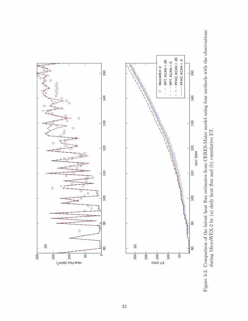
3-2 Comparison of the latent heat flux estimates from CERES-Maize model usingfour methods with the observations during MicroWEX-2 by (a) daily heat fluxand (b) cumulative ET. . . . . . . . . . . . . . . . . . . . . . . . . . . . . . . . 33

3-3 Comparison of the CERES-Maize soil moisture estimates with MicroWEX-2observations at depths of (a) 0-5 cm, (b) 5-15 cm, (c) 15-30 cm, (d) 30-45 cm,(e) 45-60 cm, and (f) 60-90 cm. . . . . . . . . . . . . . . . . . . . . . . . . . . . 35

3-4 Comparison of the CERES-Maize soil temperature estimates with MicroWEX-2observations at depths of (a) 0-5 cm, (b) 5-15 cm, (c) 15-30 cm, (d) 30-45 cm,(e) 45-60 cm, and (f) 60-90 cm. . . . . . . . . . . . . . . . . . . . . . . . . . . . 36

4-1 Surface resistance network to estimate sensible and latent heat fluxes in the LSPmodel. . . . . . . . . . . . . . . . . . . . . . . . . . . . . . . . . . . . . . . . . . 42

4-2 Algorithm for the coupling of the LSP and DSSAT models. . . . . . . . . . . . . 47

4-3 Pareto fronts from calibration of the stand-alone LSP model. The asterisk representsthe point on the Pareto front where the total seasonal RMSD for 2 cm VSM is0.04 m3/m3. . . . . . . . . . . . . . . . . . . . . . . . . . . . . . . . . . . . . . . 51

4-4 Comparison of estimations by the coupled LSP-DSSAT and stand-alone DSSATmodel simulation and those observed during MicroWEX-2: (a) dry biomass, (b)LAI, (c) 5 cm soil moisture, and (d) ET. . . . . . . . . . . . . . . . . . . . . . . 54

8

4-5 Comparison of net radiation, between DoY 78 to 105, estimated by the coupledLSP-DSSAT and stand-alone DSSAT model simulation and those observed duringMicroWEX-2: (a) values and (b) residuals . . . . . . . . . . . . . . . . . . . . . 56

4-6 Comparison of latent heat flux, between DoY 78 to 105, estimated by the coupledLSP-DSSAT and stand-alone DSSAT model simulation and those observed duringMicroWEX-2: (a) values and (b) residuals . . . . . . . . . . . . . . . . . . . . . 57

4-7 Comparison of sensible heat flux, between DoY 78 to 105, estimated by the coupledLSP-DSSAT and stand-alone DSSAT model simulation and those observed duringMicroWEX-2: (a) values and (b) residuals . . . . . . . . . . . . . . . . . . . . . 58

4-8 Comparison of soil heat flux, between DoY 78 to 105, estimated by the coupledLSP-DSSAT and stand-alone DSSAT model simulation and those observed duringMicroWEX-2: (a) values and (b) residuals . . . . . . . . . . . . . . . . . . . . . 59

4-9 Comparison of volumetric soil moisture estimated by the coupled LSP-DSSATand stand-alone LSP model simulation and those observed during MicroWEX-2,between DoY 78 to 105: (a) 2 cm, (b) 4 cm, (c) 8 cm, (d) 32 cm, (e) 64 cm,and (f) 100 cm. . . . . . . . . . . . . . . . . . . . . . . . . . . . . . . . . . . . . 60

4-10 Comparison of soil temperature estimated by the coupled LSP-DSSAT and stand-aloneLSP model simulation and those observed during MicroWEX-2, between DoY78 to 105: (a) 2 cm, (b) 4 cm, (c) 8 cm, (d) 32 cm, (e) 64 cm, and (f) 100 cm. . 61



4-13 Comparison of sensible heat flux, between DoY 105 to 125, estimated by thecoupled LSP-DSSAT and stand-alone DSSAT model simulation and those observedduring MicroWEX-2: (a) values and (b) residuals . . . . . . . . . . . . . . . . . 64



9

4-16 Comparison of soil temperature estimated by the coupled LSP-DSSAT and stand-aloneLSP model simulation and those observed during MicroWEX-2, between DoY105 to 125: (a) 2 cm, (b) 4 cm, (c) 8 cm, (d) 32 cm, (e) 64 cm, and (f) 100 cm. 67



4-19 Comparison of sensible heat flux, between DoY 125 to 135, estimated by thecoupled LSP-DSSAT and stand-alone DSSAT model simulation and those observedduring MicroWEX-2: (a) values and (b) residuals . . . . . . . . . . . . . . . . . 70








10

4-27 Comparison of fluxes estimated by the coupled LSP-DSSAT and stand-aloneLSP model simulation and those observed during MicroWEX-2: (a) net radiation,(b) latent heat flux, (c) sensible heat flux, and 2 cm soil heat flux. . . . . . . . . 78

4-28 Comparison of volumetric soil moisture estimated by the coupled LSP-DSSATand stand-alone LSP model simulation and those observed during MicroWEX-2:(a) 2 cm, (b) 4 cm, (c) 8 cm, (d) 32 cm, (e) 64 cm, and (f) 100 cm. . . . . . . . 79

4-29 Comparison of soil temperature estimated by the coupled LSP-DSSAT and stand-aloneLSP model simulation and those observed during MicroWEX-2: (a) 2 cm, (b) 4cm, (c) 8 cm, (d) 32 cm, (e) 64 cm, and (f) 100 cm. . . . . . . . . . . . . . . . . 80

5-1 Observations of total and ear wet biomass during (a) MicroWEX-4 in 2005 and(b) MicroWEX-5 in 2006. . . . . . . . . . . . . . . . . . . . . . . . . . . . . . . 83

5-2 Observations of canopy height during (a) MicroWEX-4 in 2005 and (b) MicroWEX-5in 2006. . . . . . . . . . . . . . . . . . . . . . . . . . . . . . . . . . . . . . . . . 84

5-3 Cloud densities measured during (a) MicroWEX-4 in 2005 and (b) MicroWEX-5in 2006. The symbols and the lines represent the measurements and the bestcurve-fits, respectively. . . . . . . . . . . . . . . . . . . . . . . . . . . . . . . . . 85

5-4 Moisture mixing ratios measured during (a) MicroWEX-4 in 2005 and (b) MicroWEX-5in 2006. . . . . . . . . . . . . . . . . . . . . . . . . . . . . . . . . . . . . . . . . 86

5-5 Comparison of τ calculated using the biophysical τ model (with and withoutthe gaussian term) and that using the Jackson model during (a) MicroWEX-4in 2005, and (b) MicroWEX-5 and 2006. . . . . . . . . . . . . . . . . . . . . . . 89

5-6 Comparison of the observed TB at H-pol during MW5 those simulated by theMB model using τ from the biophysical model and from the Jackson model duringlate-season MicroWEX-5. . . . . . . . . . . . . . . . . . . . . . . . . . . . . . . 90

5-7 Comparison of microwave brightness, estimated by the LSP-DSSAT-MB modelwith specular surface (a) and Wegmuller and Matzler (b), and C-band microwavebrightness observed during MicroWEX-2, before DoY 125. . . . . . . . . . . . . 92

5-8 Comparison of microwave brightness, estimated by the LSP-DSSAT-MB modelwith specular surface (a) and Wegmuller and Matzler (b), and C-band microwavebrightness observed during MicroWEX-2, after DoY 125. . . . . . . . . . . . . . 93

11

Abstract of Thesis Presented to the Graduate Schoolof the University of Florida in Partial Fulfillment of theRequirements for the Degree of Master of Engineering

MODELING LAND SURFACE FLUXES AND MICROWAVE SIGNATURES OFGROWING VEGETATION

By

Joaquin J. Casanova

December 2007

Chair: Jasmeet JudgeMajor: Agricultural and Biological Engineering

Soil moisture in the root zone is an important component of the global water and

energy balance, governing moisture and heat fluxes at the land surface and at the

vadose-saturated zone interface. Typically, soil moisture estimates are obtained using

Soil-Vegetation-Atmosphere Transfer (SVAT) models. However, two main challenges

remain in SVAT modeling. First, most models often oversimplify the coupling between

vegetation growth and surface fluxes, and second, model errors accumulate due to

uncertainty in parameters and forcings, and numerical computation. The ultimate goal

of this research is to improve estimates of root-zone soil moisture and ET by linking an

SVAT model with a crop growth model, and assimilating remotely-sensed observations

sensitive to soil moisture, such as microwave brightness (MB). Toward that goal, a coupled

SVAT-Crop model will be developed, calibrated, and linked to an MB model, to comprise

the forward model for data assimilation. The models will use observations from three

season-long field experiments monitoring growing sweet corn.

12

CHAPTER 1INTRODUCTION

Soil moisture in the root zone is an important component of the global water and

energy balance, governing moisture and heat fluxes at the land surface and at the

vadose-saturated zone interface. Typically, soil moisture estimates are obtained using

Soil-Vegetation-Atmosphere Transfer (SVAT) models. SVAT models simulate energy

and moisture transport in soil and vegetation and estimate the fluxes at the land surface

and in the root zone. Some widely-used SVAT models include the Common Land Model

(CLM) [10], the model developed by the National Centers for Environmental Prediction at

Oregon State University, Air Force, and Hydrologic Research Laboratory at the National

Weather Service (NOAH) [46], and the University of Michigan Microwave Geophysics

Group Land Surface Process (LSP) model [38]. However, two main challenges remain in

modeling energy and moisture fluxes using SVAT models.

First, most models often oversimplify the coupling between vegetation growth and

surface fluxes. The interactions between vegetation and the fluxes become increasingly

important as these fluxes affect plant growth and development. Vegetation canopies

impact latent and sensible heat fluxes, precipitation interception, and radiative transfer

at the land-atmosphere interface, affecting soil moisture and temperature profiles in the

vadose zone. These changing interactions during the growing season need to be included

in the SVAT models, in order to provide realistic estimates of the fluxes. Typically, SVAT

models employ observations or empirical functions for vegetation conditions to model

the effects of growing vegetation. For example, CLM uses vegetated grid spaces defined

by patches of “plant functional types,” with parameters for physiological and structural

properties associated with each type, and most of the vegetation parameters are empirical

to meet computational constraints [10]. NOAH simulates soil moisture and temperature

profiles with a sub-daily timestep, and with vegetation properties such as LAI, stomatal

resistance, and roughness length defined by vegetation type classes [46]. Such methods

13

ignore the interaction between surface fluxes and vegetation growth. Second, SVAT model

estimates of fluxes, soil moisture, and soil temperature diverge from observations due to

uncertainty in parameters, forcings, and initial conditions, and due to accumulated errors

from numerical computation.

SVAT models can be coupled with crop growth models to include dynamic interactions

between the vegetation growth and flux estimates. For example, [23] used a sub-daily

biochemical vegetation model with a land surface hydrology model. They modeled

canopy transpiration and its influence on soil moisture and carbon fluxes. [41] linked

daily process-based crop models for summer maize and winter wheat with an hourly

land surface flux model and a three-layer soil moisture model. Such coupling allows for

inclusion of vegetation effects without in situ observations or empirical growth functions.

Periodic in situ observations of vegetation could be incorporated in the coupled models to

reduce the divergence of model prediction from reality.

Remotely-sensed observations sensitive to soil moisture, such as low frequency (< 10

GHz) microwave brightness (TB) [15, 26, 43, 52] could also be incorporated periodically

to improve model flux estimates. To incorporate or assimilate microwave brightness,

the coupled SVAT-crop model has to be linked to a microwave emission model that

estimates microwave brightness using moisture and temperature profiles in soil and

vegetation estimated by the SVAT-Crop model as shown in Figure 1-1. Simple versions of

SVAT models linked with MB models include the Land Surface Process/Radiobrightness

(LSP/R) [30] and Simple Soil-Plant-Atmosphere Transfer - Remote Sensing (SiSPAT-RS)

[12] models.

The total TB of a terrain is dependent on sky TB, reflected by the soil (TB,sky),

thermal emission from the soil (TB,soil, and thermal emission from the vegetation canopy

(TB,canopy, all three components are shown in Figure 1-2). Since soil microwave emissions

(dependent on soil moisture and temperature profiles) are attenuated by transmission

14

Figure 1-1. Outline of the data assimilation scheme and the forward model.

Figure 1-2. Contributions to microwave brightness TB from sky, soil, and canopy.

15

through the canopy, a microwave transmission model for growing vegetation is an

important component of the MB model.

Microwave emission models for dynamic vegetation during the growing season require

accurate estimation of canopy emission and attenuation. Non-scattering attenuation is

described by canopy optical depth (τ) that primarily depends upon the distribution of

moisture in the canopy. Several methods have been investigated for determining canopy

optical depth. For example, Ulaby and Wilson[58] modeled τ of the wheat canopy as

a uniform cloud of wet biomass with leaves and stems treated separately. In addition,

polarization dependence was included for stem attenuation. Eom [21] developed a model

for τ applicable to row structured canopies such wheat or corn. The model accounts for

azimuthal anisotropy in τ by modeling the canopy as a random collection of dielectric

spheroids. This method matched well with observations but requires a computationally

intensive solution of the radiative transfer equation. Jackson and Schmugge [51], used

the results of many studies and developed an empirical model for τ . In their model, τ is

estimated as the product of a frequency-dependent constant b and water column density

(kg/m2) in the canopy. The Jackson model is flexible but has little physical basis, with

b often used as a fitting parameter in emission models or estimated empirically [61].

England and Galantowicz [19] developed a refractive model for estimating optical depth of

grass based upon vertical profiles of moisture content within the grass canopy.

In this thesis, an SVAT model, viz. the LSP model, is coupled with a widely-used and

well-tested crop growth model, the Decision Support System for Agrotechnology Transfer

Cropping System Model (DSSAT-CSM) [29]. The models are calibrated using obserations

from the Microwave Water and Energy Balance Experiment 2 (MicroWEX-2), one of three

season-long experiments monitoring growing sweet corn (MicroWEXs 2, 4, and 5). A

biophysically-based canopy transmission model is developed for growing sweet corn, using

data from MicroWEXs 4 and 5. This τ model is included in a simple MB model that is

linked with the LSP-DSSAT model.

16

1.1 Thesis Objectives

This thesis answers the following research questions:

1. What values for the six corn cultivar coefficients give the best DSSAT model

performance for both biomass and LAI for the MicroWEX-2 growing season?

(Chapter 3)

2. How do the model estimates for biomass and LAI compare with MicroWEX-2

observations? (Chapter 3)

3. What values of the twelve calibrated parameters give the best LSP model performance

for both latent heat flux and near surface soil moisture for the MicroWEX-2 growing

season? (Chapter 4)

4. How do the model estimates of soil moisture, temperature, and surface fluxes

compare with MicroWEX-2 observations? (Chapter 4)

5. What is the impact of coupling on both LSP and DSSAT model estimates of LAI,

biomass, soil moisture, temperature, and surface fluxes? (Chapter 4)

6. How does a physically-based τ model compare to Jackson’s widely-used empirical

model? (Chapter 5)

7. How do the brightness estimates predicted by the linked LSP-DSSAT-MB model

compare to observations during MicroWEX-2? (Chapter 5)

1.2 Thesis Format

The Chapter 2 of this thesis describes the field experiments, MicroWEXs 2, 4, and

5. In Chapter 3, the DSSAT model’s corn submodel, CERES-Maize, is calibrated for the

MicroWEX-2 growing season. In Chapter 4, the LSP model is calibrated and coupled

with DSSAT model. In Chapter 5, a canopy transmission model for growing sweet corn is

developed and tested in a simpled MB model, linked with the LSP-DSSAT model.

17

CHAPTER 2MICROWAVE WATER AND ENERGY BALANCE EXPERIMENTS

The MicroWEXs are a series of experiments conducted by the Center for Remote

Sensing at the University of Florida during growing seasons of corn and cotton [6, 8, 33,

37, 55, 67]. The objective of the experiments are to understand microwave signatures of

agricultural crops during different stages of growth. MicroWEX-2 was conducted during

the sweet corn growing season, from March 18 through June 2 in 2004 [33]. MicroWEX-4

was conducted during the sweet corn growing season, from March 10 through June 2 in

2005 [6]. MicroWEX-5 was conducted during the subsequent corn season from March 9

through May 26 in 2006 [8]. All experiments were conducted at the same 37,000 m2 site

in UF/IFAS Plant Science Research and Education Unit in Citra, FL (29.41 N, 82.18

W). The soils at the site are Lake Fine Sand with about 90 % sand and a bulk density of

1.55 g/cm3. Row spacing was 76 cm, with approximately eight plants per square meter.

Irrigation and fertigation were conducted via a linear move system.

Data collected during the MicroWEXs included soil moisture, temperature and

heat flux, latent and sensible heat flux, wind speed and direction, upwelling and

downwelling short and longwave radiation, precipitation, irrigation, water table depth,

and vertically and horizontally polarized microwave brightness at 6.7 GHz (λ = 4.47 cm),

every fifteen minutes using the tower-mounted University of Florida C-band Microwave

Radiometer (UFCMR, Figure 2-1). Additional horizontally polarized microwave brightness

observations at 1.4 GHz (λ = 21.4 cm) were conducted during MicroWEX-5 using the

UF L-Band Microwave Radiometer (UFLMR, Figure 2-2). The radiometer frequencies, at

6.7 GHz and at 1.4 GHz, correspond to the lowest frequency of the Advanced Scanning

Microwave Radiometer (AMSR-E) [22], and the frequency of the planned Soil Moisture

and Ocean Salinity (SMOS) mission [34], respectively.

The soil moisture, heat fluxes, and temperatures were observed at three locations

in the field. Soil moisture and soil temperature were observed at 2, 4, 8, 16, 32, 64,

18

Figure 2-1. The University of Florida C-band Microwave Radiometer.

Figure 2-2. The University of Florida L-band Microwave Radiometer.

19

Figure 2-3. The Eddy Covariance System.

Figure 2-4. The net radiometer used during the MicroWEXs.

and 120 cm (100 cm during MicroWEX-2) using Campbell Scientific Water Content

Reflectometers and Vitel Hydra- probes; and thermistors and thermocouples, respectively.

An Eddy Covariance System (Figure 2-3) measured wind speed, direction, and latent and

sensible heat fluxes. REBS CNR net radiometer (Figure 2-4)measured up- and down-

welling short- and longwave radiation. Everest Interscience infrared sensor measured

thermal infrared temperature. Four tipping-bucket rain gauges logged precipitation at

four locations East and West of the footprint, and at the East and West sides of the field.

Water table depth was measured using Solinst Level Loggers in a monitoring well in each

quadrant.

In addition to continuously logged data, there were also weekly vegetation and

twice-weekly soil samplings (during MicroWEX-2 only). Vegetation sampling was

conducted in four areas, one in each quadrant of the field. Samples were selected by

placing a meter stick half-way between two plants and ending the sample at least 1 m

from the starting point and half-way between two plants. The actual row length of the

sample was noted. Stand density, leaf number, canopy height and width, wet and dry

20

weights of leaves, stems, and ears were measured. Two LAI measurements were taken

in each sampling area using the Licor LAI-2000 Canopy Analyzer. Vertical distribution

of moisture in the canopy was measured five times during MicroWEX-4 and three times

during MicroWEX-5 [7]. During soil sampling, soil moisture and temperatures were

observed in-row and in-furrow at depths of 2, 4, and 8 cm along eight transects at ten

to thirteen locations, using the Delta-T ThetaProbe soil moisture sensor and a digital

thermometer to quantify the spatial variability of the field. Vegetation and soil nitrogen

(as NH+4 and NO−

3 ) were measured in each of the four sampling areas. Root length density

was measured in the vadose zone at tasseling.

21

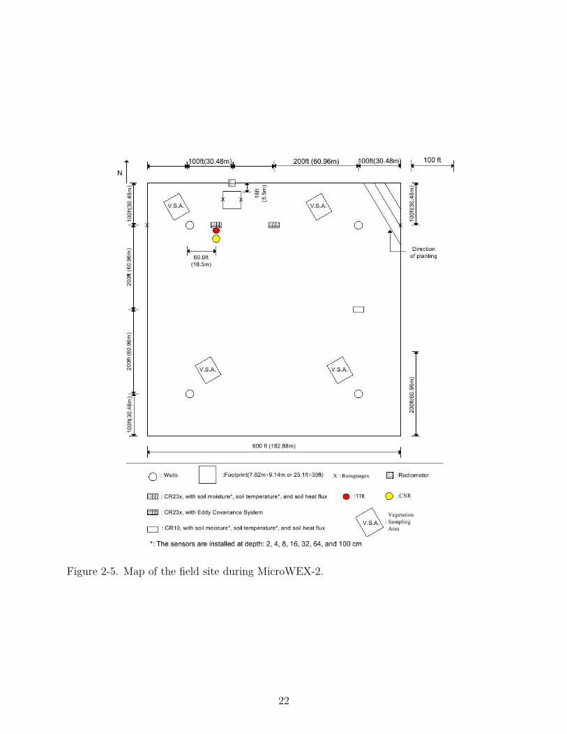
Figure 2-5. Map of the field site during MicroWEX-2.

22


23


24

CHAPTER 3CALIBRATION OF A CROP GROWTH MODEL FOR SWEET CORN

3.1 Introduction

This chapter describes the calibration of a crop growth model for a growing season

of sweet corn in north-central Florida. There are two major corn growth models, EPIC

(Erosion Productivity Impact Calculator) [65] and CERES-Maize [28], that simulate

hydrology, nutrient cycling, growth, and development. CERES-Maize has the advantage

of being part of the well-known Decision Support System for Agrotechnology Transfer

Cropping System Model (DSSAT-CSM). DSSAT has been widely used for a number of

years, with validated models for over 15 crops. It also allows for simulations of multi-year

crop rotations [29].

3.2 CERES-Maize Model

The CERES-Maize model is a part of the crop growth submodule in DSSAT-CSM.

DSSAT-CSM is a modular crop simulation model with modules for soil, soil-plant-atmosphere,

crop development and growth, weather, management, etc. A simulation consists of several

stages: season and run initialization, rate calculation, integration, and output generation

[29]. The model determines total dry biomass using the radiation use efficiency method.

Total solar radiation is partitioned into photosynthetically active radiation (PAR), and

the fraction intercepted is calculated from LAI using Beer’s law [54]. The dry matter

accumulation rate is a product of radiation use efficiency and a conversion factor. Maize

growth and development is marked by eight events: germination, emergence, end of

juvenile phase, floral induction (tassel initiation), 75% silking, beginning grain fill,

maturity, and harvest. Transition from one developmental stage to the next is determined

by the growing degree days (GDD) with a base temperature of 8C. Vegetative growth

stops on 75% silking, when reproductive growth begins in the form of grain fill. Yield is

the grain fill value at harvest. Threshold GDD for each stage and grain fill parameters are

contained in a cultivar file.

25

The CERES-Maize model determines LAI by tracking the total number of leaves and

calculating a leaf area growth rate, so that the rate of increase of LAI is the product of

leaf area growth and current leaf number. Leaf growth is partly determined by the number

of degree days between successive leaf tip appearances, called the phyllochron interval. In

addition, a leaf senescence rate is calculated based on water stress.

The soil-plant-atmosphere module estimates ET at the land surface using either

the Ritchie-modified Priestley-Taylor (RPT) method [48] or the Penman-FAO (PFAO)

method [14]. The RPT method depends only on solar radiation and temperature, while

the PFAO method accounts for wind speed and relative humidity as well. Both methods

first determine a total potential ET, which is partitioned into potential soil evaporation

and potential plant transpiration. Potential soil evaporation is based on intercepted solar

radiation reaching the soil surface as a function of temperature, wind speed, radiation,

and humidity. Potential plant transpiration depends on the radiation intercepted by the

canopy and temperature, wind speed, and humidity. Actual evaporation and transpiration

are determined by the minimum of potential ET and the amount of available water. For

soil evaporation, surface soil water is the limiting factor, while for transpiration, root water

uptake is the limiting factor.

The soil is divided into nine layers, each with different constitutive properties.

Soil moisture is calculated using the bucket method [39]. When an upper soil layer is

above the drained upper limit, excess flows to the one below, in addition to computing

estimates for capillary rise. Runoff is calculated using the USDA Soil Conservation Service

runoff number method [53]. Infiltration is equal to excess precipitation after runoff. Soil

temperature is computed using a deep soil boundary condition and an air temperature

boundary condition. The air temperature (C) is calculated from the average of maximum

and minimum daily temperatures. Soil temperature (ST ) varies with soil layer (L) as [29]:

ST (L) = TAV G + (TAMP

2.0COS(ALX + ZD) +DT )eZD (3–1)

26

where DT is the difference between the average of the daily average temperatures

during the previous five days and the yearly average (C), ZD is depth (cm), TAMP is

amplitude of yearly temperature (C), and ALX is the difference in days from the current

day to the hottest day of the year.

3.3 Model Calibration

The CERES-Maize model was ported to the Linux OS and calibrated using data from

MicroWEX-2. This section describes the calibration procedure.

3.3.1 Initialization

CERES is the crop submodule for cereal crops, including maize. CERES-Maize uses

three files for determining growth and development characteristics: the species file, the

ecotype file, and the cultivar file. The species file contains defining characteristics of

corn, including root growth parameters, seed initial conditions, nitrogen and water stress

response coefficients, nitrogen uptake parameters, base and optimum temperatures for

grain fill and photosynthesis, and radiation and CO2 parameters governing photosynthesis.

The ecotype file specifies thermal time development, radiation use efficiency, and light

extinction coefficients for three main types of corn. The cultivar file specifies the cultivar

coefficients that describe the growth and development characteristics for different maize

cultivars. These are:

P1: degree days between emergence and end of juvenile stage.

P2: development delay for each hour increase in photoperiod past optimum

photoperiod.

P5: degree days from silking to maturity.

G2: maximum possible number of kernels per plant.

G3: kernel filling rate during the linear grain filling stage and under optimum

conditions (mg/day).

PHINT: phyllochron interval, i.e., the interval in thermal time (degree days) between

leaf tip appearances.

27

Soil properties such as hydraulic conductivity and texture were taken as the default

values for the soil type that most closely corresponds with our field site (Millhopper fine

sand) and that is included in the DSSAT soil properties file. The drained lower limit

of the top nine soil layers was set to the minimum soil moisture (0.05) observed during

MicroWEX-2. The initial soil moisture for all the layers was set equal to 0.2. The model

calibration was found to be insensitive to the choice of initial moisture conditions because

an irrigation event that occurred at planting reset the soil moisture profile of sandy soil.

3.3.2 Inputs

Most of the inputs for the model calibration were obtained from the MicroWEX-2

dataset. These included daily incoming solar radiation, precipitation, irrigation,

fertigation, and wind speed. Maximum and minimum daily temperature and relative

humidity were obtained from the micrometeorological dataset collected for the Agricultural

Field-Scale Irrigation Requirement Simulation (AFSIRS) study at a nearby site at the

PSREU [16].

3.3.3 Methodology

To calibrate the CERES-Maize model, a broad grid search was employed, followed by

simulated annealing in the area of the global minimum using the six cultivar coefficients.

Each coefficient was incrementally changed, so that a grid of possible combinations of

values was tested to minimize the differences between model estimates and observations

from biomass and LAI, the two most important canopy parameters required by the MB

model. The LAI observation on DoY 135 was excluded for calibration, due to its high

standard deviation (Figure 3-1a). The objective function (R) was computed as the sum of

square residuals, normalized by variance [54]:

R =SSRB

σ2B

+SSRLAI

σ2LAI

(3–2)

where SSRB is the sum of square residuals from total biomass, SSRLAI is the sum

of square residuals from LAI, and σ2B and σ2

LAI are the variances of biomass and LAI

28

Table 3-1. Cultivar coefficient values in the calibrated CERES-Maize model.

Cultivar Coefficient ValueP1 157.20P2 1.000P5 811.20G1 853.00G3 10.4PHINT 40.33

observations, respectively. The optimum combination of parameter values found by the

grid search was then used as the initial guess in a simulated annealing optimization

algorithm [2]. The root mean square difference (RMSD), relative root mean square

difference (RRMSD), and Willmott d -index [66] were calculated as for LAI and the

biomass of each component, leaves, stems, and grain:

RMSD = (Σ(Pi −Oi)

2

n)1/2 (3–3)

RRMSD =RMSD

O(3–4)

d = 1− Σ(Pi −Oi)2

Σ(|Pi − P |+ |Oi − O|)2(3–5)

where n is the number of observations, Pi and Oi are the predicted and observed

values, and P and O are the predicted and observed means. Table 3-1 shows the values of

the six cultivar coefficients that minimized R in Equation 3–2.

3.4 Results and Discussion

3.4.1 Crop Growth and Development

To evaluate the CERES-Maize model for crop growth and development, model

estimates are compared of emergence and silking dates, biomass, and LAI to the

observations during MicroWEX-2.

29

The modeled and observed emergence dates were on DoY 90 and DoY 86, respectively.

Modeled anthesis day (when 75% of the corn has silked) was DoY 139, while 75% silking

was observed by DoY 135. The model estimated realistic total dry biomass using the

parameters determined by the grid search, as shown in Figure 3-1. The RMSD for

biomass was 0.90 Mg/ha with a low RRMSD of 0.23 and a correspondingly high Willmott

d -index of 0.99, as shown in Table 3-2. Figure 3-1b shows a scatter plot of estimated

and observed total biomass. The biomass was increasingly underestimated by the model

as the season progressed, with the maximum difference of 1.41 Mg/ha at the end of the

season. The partitioning of the modeled biomass into leaf and stem biomass did not match

the observations (Figure 3-1a), as indicated by the high RMSD and RRMSD in Table

3-2. Partitioning of total biomass into stem biomass was underestimated by the model

during later vegetative stages of growth (DoY 127 to DoY 134). The partitioning into

leaf biomass was more realistic, with a slight overestimation during later growth stages

(DoY 132 to DoY 142). The model’s estimate of the beginning of grain fill at DoY 140

matched closely with the observed grain fill at DoY 139 (Figure 3-1a). The best fit for

LAI and total biomass did not produce the best fit for grain fill. In order to compensate

for the underestimated stem biomass, grain weight must be overestimated. The model

estimated realistic LAI, as seen in Figure 3-1, with a low RMSD and RRMSD of 0.22 and

0.13, respectively, and a high Willmott d -index of 0.99, as shown in Table 3-2. Figure 3-1d

shows the scatter plot of the model and observed LAI.

30

8090

100

110

120

130

140

150

024681012

Dry Biomass (Mg/ha)

(a)

Mic

roW

EX

−2

Tot

al

Mic

roW

EX

−2

Leaf

Mic

roW

EX

−2

Ste

m

Mic

roW

EX

−2

Gra

in

Mod

el T

otal

Mod

el L

eaf

Mod

el S

tem

Mod

el G

rain

02

46

810

12024681012

(b) Mic

roW

EX

−2

Bio

mas

s (M

g/ha

)

8090

100

110

120

130

140

150

0

0.51

1.52

2.53

3.54

4.5

DoY

200

4

LAI

(c)

Mic

roW

EX

−2

LAI ±

σ

Mod

el L

AI

01

23

40

0.51

1.52

2.53

3.54

4.5

Mic

roW

EX

−2

LAI

(d)

Fig

ure

3-1.

(a)

Com

par

ison

ofth

eC

ER

ES-M

aize

esti

mat

esan

dth

eob

serv

atio

ns

ofbio

mas

sduri

ng

Mic

roW

EX

-2,(b

)sc

atte

rplo

tof

esti

mat

edan

dob

serv

edbio

mas

s,(c

)co

mpar

ison

ofth

eC

ER

ES-M

aize

esti

mat

esan

dth

eob

serv

atio

ns

ofLA

Iduri

ng

Mic

roW

EX

-2,an

d(d

)sc

atte

rplo

tof

esti

mat

edan

dob

serv

edLA

I.

31

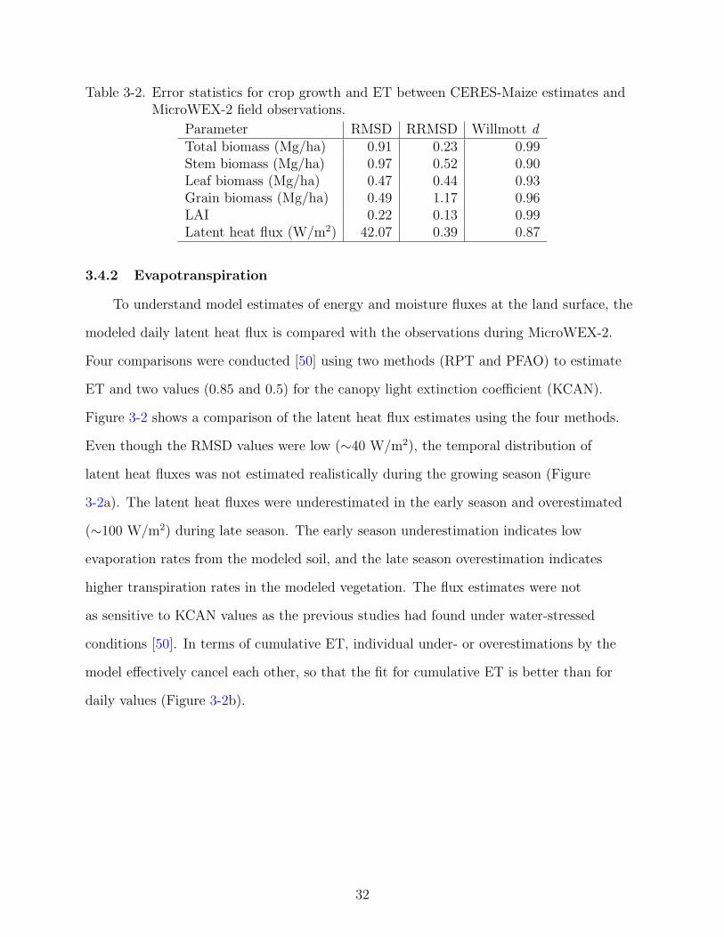
Table 3-2. Error statistics for crop growth and ET between CERES-Maize estimates andMicroWEX-2 field observations.

Parameter RMSD RRMSD Willmott dTotal biomass (Mg/ha) 0.91 0.23 0.99Stem biomass (Mg/ha) 0.97 0.52 0.90Leaf biomass (Mg/ha) 0.47 0.44 0.93Grain biomass (Mg/ha) 0.49 1.17 0.96LAI 0.22 0.13 0.99Latent heat flux (W/m2) 42.07 0.39 0.87

3.4.2 Evapotranspiration

To understand model estimates of energy and moisture fluxes at the land surface, the

modeled daily latent heat flux is compared with the observations during MicroWEX-2.

Four comparisons were conducted [50] using two methods (RPT and PFAO) to estimate

ET and two values (0.85 and 0.5) for the canopy light extinction coefficient (KCAN).

Figure 3-2 shows a comparison of the latent heat flux estimates using the four methods.

Even though the RMSD values were low (∼40 W/m2), the temporal distribution of

latent heat fluxes was not estimated realistically during the growing season (Figure

3-2a). The latent heat fluxes were underestimated in the early season and overestimated

(∼100 W/m2) during late season. The early season underestimation indicates low

evaporation rates from the modeled soil, and the late season overestimation indicates

higher transpiration rates in the modeled vegetation. The flux estimates were not

as sensitive to KCAN values as the previous studies had found under water-stressed

conditions [50]. In terms of cumulative ET, individual under- or overestimations by the

model effectively cancel each other, so that the fit for cumulative ET is better than for

daily values (Figure 3-2b).

32

8090

100

110

120

130

140

150

050100

150

200

Heat Flux (W/m2)

(a)

8090

100

110

120

130

140

150

50100

150

200

250

ET (mm)

DoY

200

4

(b)

Mic

roW

EX

−2

RP

T, K

CA

N =

.85

RP

T, K

CA

N =

.5

PF

AO

, KC

AN

= .8

5

PF

AO

, KC

AN

= .5

Fig

ure

3-2.

Com

par

ison

ofth

ela

tent

hea

tflux

esti

mat

esfr

omC

ER

ES-M

aize

model

usi

ng

four

met

hods

wit

hth

eob

serv

atio

ns

duri

ng

Mic

roW

EX

-2by

(a)

dai

lyhea

tflux

and

(b)

cum

ula

tive

ET

.

33

3.4.3 Soil Moisture and Temperature

To understand the model performance regarding moisture and energy transport

in soil, modeled daily soil moisture and temperature profiles are compared to the

observed average daily values during MicroWEX-2 (Figures 3-3, 3-4, and 3-3). To compare

observations at 2, 4, 8, 16, 32, 64, and 100 cm to model estimates of the top six layers,

the average of 2 and 4 cm observations are compared to estimates of 0-5 cm, 8 and 16

cm observations to estimates of 5-15 cm, 16 and 32 cm observations to estimates of 15-30

cm, average of 32 cm observations to estimates of 30-45 cm, 32 and 64 cm observations to

estimates of 45-60 cm, and 64 and 100 cm observations to estimates of 60-90 cm.

34

8010

012

014

00

0.050.

1

0.150.

2

0.25

0−5

cm

(a)

VSM (m3/m

3)

8090

100

110

120

130

140

150

0

0.050.

1

0.150.

2

0.25

5−15

cm

(b)

VSM (m3/m

3)

8090

100

110

120

130

140

150

0

0.050.

1

0.150.

2

0.25

15−

30 c

m

(c)

DoY

200

4

VSM (m3/m

3)

8090

100

110

120

130

140

150

0

0.050.

1

0.150.

2

0.25

30−

45 c

m

(d)

8090

100

110

120

130

140

150

0

0.050.

1

0.150.

2

0.25

45−

60 c

m

(e)

8090

100

110

120

130

140

150

0

0.050.

1

0.150.

2

0.25

60−

90 c

m

(f)

DoY

200

4

Mic

roW

EX

−2

(Dai

ly A

vera

ge)

Mod

el

Mic

roW

EX

−2

(15

min

)

Fig

ure

3-3.

Com

par

ison

ofth

eC

ER

ES-M

aize

soil

moi

sture

esti

mat

esw

ith

Mic

roW

EX

-2ob

serv

atio

ns

atdep

ths

of(a

)0-

5cm

,(b

)5-

15cm

,(c

)15

-30

cm,(d

)30

-45

cm,(e

)45

-60

cm,an

d(f

)60

-90

cm.

35

Fig

ure

3-4.

Com

par

ison

ofth

eC

ER

ES-M

aize

soil

tem

per

ature

esti

mat

esw

ith

Mic

roW

EX

-2ob

serv

atio

ns

atdep

ths

of(a

)0-

5cm

,(b

)5-

15cm

,(c

)15

-30

cm,(d

)30

-45

cm,(e

)45

-60

cm,an

d(f

)60

-90

cm.

36

Table 3-3. model performance statistics for soil moisture and temperature betweenCERES-Maize estimates and MicroWEX-2 field observations.

RMSDLayer Soil Moisture Soil Temperature (K)5-15 cm 0.0204 2.53415-30 cm 0.0344 1.42630-45 cm 0.0164 1.48545-60 cm 0.0117 2.77560-90 cm 0.0083 3.648

The CERES-Maize model simulates moisture at daily timesteps, while the hydrological

changes near the soil surface (0-5 cm) occur at much shorter timesteps, making it

challenging to compare model and observed near-surface soil moisture. In Figure 3-3a, the

daily moisture at 0-5 cm estimated by the CERES-Maize model is compared with daily

averages and 15 min observations of volumetric soil moisture (VSM) during MicroWEX-2.

Deeper soil layers matched the observed values fairly well, as suggested by their low

RMSD values in Table 3-3, except for a 2% underestimation during the entire growing

season for the 15-30 cm layer. This is within the experimental error of the observations

made by the TDR probes.

Overall, the model did not capture the changes in soil temperatures realistically

during the growing season. It estimated temperatures at depths of 15-45 cm fairly well,

as indicated by their low RMSD values in Table 3-3. The temperatures at deeper layers

were underestimated throughout the growing season, with increasing differences as the

season progressed. For the upper layers, the model did not capture the strong fluctuations

in temperature closer to the surface.

3.5 Summary

This chapter answers the first two research questions from Chapter 1.

Question 1:”What values for the six corn cultivar coefficients give the best

DSSAT model performance for both biomass and LAI for the MicroWEX-2

growing season?”

37

The calibrated cultivar coefficient values which give the best estimates for biomass

and LAI are given in Table 3-1.

Question 2:”How do the model estimates for biomass and LAI compare with

MicroWEX-2 observations?”

The RMSD for biomass was 0.90 Mg/ha. The biomass was increasingly underestimated

by the model as the season progressed, with the maximum difference of 1.41 Mg/ha at the

end of the season. The model estimated realistic LAI with a low RMSD of 0.22.

38

CHAPTER 4CALIBRATION OF AN SVAT MODEL AND COUPLING WITH A CROP MODEL

FOR SWEET CORN

4.1 Introduction

This chapter describes the coupling of an SVAT model with a crop growth simulation

model to estimate land surface fluxes in growing vegetation and evaluate the performance

of the coupled model for estimating root-zone soil moisture and ET observations from

an extensive field experiment. Both categories of models benefit from two decades of

development and testing by their respective research communities. The SVAT model,

viz. Land Surface Process (LSP) model, simulates one-dimensional energy and moisture

transport as well as radiative, sensible and latent heat fluxes at the land surface. The

cropping system model, viz. the Decision Support System for Agrotechnology Transfer

(DSSAT), is a widely-used and tested modular suite of crop models that simulate crop

growth (biomass accumulation) and development (vegetative and reproductive growth

stages). Neither model is structurally changed and an interface is created to link the two

models. In the coupled LSP-DSSAT model, the DSSAT model provides the LSP model

with vegetation characteristics that influence heat, moisture, and radiation transfer at the

land surface and in the vadose zone and the LSP model provides the DSSAT model with

estimates of soil moisture and temperature profiles and evapotranspiration (ET).

4.2 LSP Model

The LSP model was originally developed by the Microwave Geophysics Group at

the University of Michigan [38]. The model simulates 1-d coupled energy and moisture

transport in soil and vegetation, and estimates energy and moisture fluxes at the land

surface and in the vadose zone. It is forced with micrometeorological parameters

such as air temperature, relative humidity, downwelling solar and longwave radiation,

irrigation/precipitation, and windspeed. The original version has been rigorously tested

[31] and extended to wheat stubble [30] and brome-grass [32], prairie wetlands in Florida

[64], and tundra in the Arctic [9] .

39

A new version of the LSP model was used with a modified radiation flux parameterization

at the land surface. Specifically, the shortwave radiative transfer was altered to a more

physically-based formulation, including both diffuse and direct radiation, and canopy

transmissivity described by Campbell and Norman [4]. The original version of the LSP

model followed a more empirically-based formulation by Verseghy et al. [62]. In addition,

the aerodymanic resistances and the surface vapor resistances were changed in the new

version to extend it to tall vegetation and to partially-vegetated terrain [24]. The original

version was developed for homogeneous land cover, such as bare soil or short grass. The

new version of the model also includes adaptive timesteps for computational efficiency and

to allow sudden changes or large fluxes in the sandy soils with high thermal and hydraulic

conductivities. The following section provides a detailed description of the modified LSP

model used in this study. Some fundamental governing equations are also included in the

section for completeness even though they remain unchanged from the original version.

4.2.1 Energy and Moisture Transport at the Land Surface

4.2.1.1 Energy Balance

Combining the radiation and heat flux boundary conditions, the net energy flux into

the canopy (Qnet,c) and soil (Qnet,s) (W/m2):

Qnet,c = Hsc +Rs,c +Rl,c −Hca − LEtr − LEev (4–1)

Qnet,s = −Hsc +Rs,s +Rl,s −Hsa − LEs (4–2)

where Hsc, Hca, and Hsa are the sensible heat fluxes between soil and canopy, canopy and

air, and soil and air, respectively; LEtr, LEev, and LEs are the latent heat fluxes from

transpiration, canopy evaporation, and soil evaporation, respectively; and Rs,c, Rs,s, Rl,c,

Rl,s, are the net solar radiation intercepted by the canopy, intercepted solar radiation by

the soil, net longwave radiation at the canopy, and net longwave at the soil, respectively.

Solar Radiation (Rs,c and Rs,s)

40

Downwelling solar radiation is partitioned between the soil and canopy by first

dividing total solar radiation into direct and diffuse components, as an empirical function

of clearness index and apparent solar time [1]. The direct fraction is either transmitted,

reflected, or absorbed. The net solar radiation absorbed by the canopy and soil are

Rs,c = [(1− fd)(1− τc,dir)(1− ρc,dir) + (fd)(1− τc,diff )(1− ρc,diff )]Rs,down (4–3)

Rs,s = (1− ρs)[(1− fd)(τc,dir)(1− ρc,dir) + (fd)(τc,diff )(1− ρc,diff )]Rs,down (4–4)

where fd is the diffuse fraction, τc,dir is the direct canopy transmissivity, τc,diff is the

diffuse canopy transmissivity, ρc,dir is the direct canopy reflectance, ρc,diff is the diffuse

canopy reflectance, ρs is the soil reflectance, and Rs,down is the downwelling solar radiation.

The direct canopy transmissivity is τc,dir, given by Campbell and Norman [4]:

τc,dir = e−K(x,Θ)√

1−σΩLAI (4–5)

where K(x,Θ) is the canopy extinction coefficient for canopy with an ellipsoidal leaf

angle distribution, σ is the reflectance of a single leaf, x is the leaf angle distribution

parameter, Θ is the solar zenith angle, LAI is the leaf area index of the canopy, and Ω is

the clumping factor which accounts for incomplete canopy cover.

The canopy reflectance is calculated as

ρc,dir =2K(x,Θ)

1 +K(x,Θ)

1−√1− σ

1 +√

1− σ(4–6)

The diffuse canopy transmissivity, τc,diff , is found by integrating τc,dir over all solar zenith

angles. Diffuse canopy reflectance ρc,diff is given by Goudriaan [24]:

ρc,diff =1−√1− σ

1 +√

1− σ(4–7)

Radiation transmitted by the canopy is either reflected or absorbed by the soil according

to the soil albedo, ρs, an empirical function of soil moisture, derived from MicroWEX-2

41

Figure 4-1. Surface resistance network to estimate sensible and latent heat fluxes in theLSP model.

bare-soil data:

ρs = 0.0854e[−max(θs−0.0532,0)2/0.0037] + 0.14650 (4–8)

where θs is the surface volumetric soil moisture (m3/m3).

Longwave Radiation (Rl,c and Rl,s)

The net longwave radiation abosrbed by the canopy (Rl,c) and soil (Rl,s) are given by

Kustas and Norman [35]:

Rl,c = (1− τl)Rl,down + (1− τl)εsσsbT4s − 2(1− τl)εcσsbT

4c (4–9)

Rl,s = (τl)Rl,down − εsσsbT4s + (1− τl)εcσsbT

4c (4–10)

where σsb is the Stefan-Boltzmann constant, Rl,down is the downwelling longwave radiation,

εs is the soil emissivity, εc is the canopy emissivity, and Ts and Tc are the soil and canopy

temperatures in Kelvin. τl is the longwave canopy transmissivity, the integral over the

hemisphere of direct transmissivity with σ as zero.

Sensible Heat Fluxes

Figure 4-1(a) shows the resistance network model used to estimate sensible heat flux

(H) at the surface.The sensible heat fluxes between the soil and air (Hsa), soil and canopy

42

(Hsc), and canopy and air (Hca), are calculated as:

Hsa = ρacpaTs − Ta

ras

fB (4–11)

Hsc = ρacpaTs − Tc

rsc + rbh

fV (4–12)

Hca = ρacpaTs − Tc

rac + rbh

fV (4–13)

where Ta, Ts,and Tc are the air, soil, and canopy temperatures (K), respectively, ρa is the

air density (kg/m3), cpa is the specific heat (J/kg K), fV and fB are the vegetation and

bare soil cover fractions, respectively.

The aerodynamic resistances ras (soil-air) and rac (canopy-air) are determined

assuming a log wind profile above the canopy or bare soil [24]:

ras =ln

(z

zob

)+ ΨH

ku∗(4–14)

rac =ln

(z−dzov

)+ ΨH

ku∗(4–15)

u∗ =ku(z)

ln(

z−dzo

)+ ΨM

(4–16)

where u∗ is the friction velocity, Ψ is the Businger-Dyer stability function [17], k is von

Karman’s constant (0.4), z is the measurement height, d is the vegetation displacement

height (taken as 0.63hc, hc is the plant canopy height), zov is the vegetation roughness

length (0.1hc), and zob is the bare soil roughness length.

For the aerodynamic resistance between the soil and the canopy, the log profile is not

valid due to momentum absorption by the canopy elements, so an exponential wind profile

in the canopy is used [24], with the under-canopy resistance, rsc, from Niu and Yang [42]:

rsc =hc

aKh

[ea(1−zob/hc) − ea(1−zov/hc)] (4–17)

43

where a and Kh are the canopy damping coefficient and the aerodynamic conductance for

heat at the top of the canopy [24], given by:

a =

√cdLAIhc

2lmiw(4–18)

where

lm = 23

√0.75w2

chc

πLAI(4–19)

Kh = ku∗(hc − d) (4–20)

where, lm is the canopy momentum length, iw is the wind intensity factor, cd is the drag

coefficient, and wc is canopy width. The leaf boundary layer resistances for heat transport,

rbh, is calculated as:

rbh =1

2(180)

√lwuc

(4–21)

uc = ku∗ln(hc − d

zov

)(4–22)

Latent Heat Flux

Latent heat flux is based upon the resistance network (see Figure 4-1(b)). Three

sources that contribute to the flux are: soil evaporation (LEs), canopy transpiration

(LEtr), and evaporation of intercepted precipitation (LEev).

LEs = λρa(qs − qa)

(fV

rs + rsc + rca

+fB

rs + ras

)(4–23)

LEtr = λρa(qc,sat − qa)

[fV (1− xl)

rac + rbv + rlv

](4–24)

LEev = λρa(qc,sat − qa)fV xl

rac + rbv

(4–25)

where qa, qs, and qc,sat are the specific humidities of the air, soil surface layer, and

saturated canopy, respectively, λ is the latent heat of vaporization of water, and xl is

the fraction of vegetation covered in intercepted precipitation, calculated by

xl =Wr

Wr,max

(4–26)

44

Wr,max = 0.2LAI (4–27)

where Wr,max is the maximum possible interception, and Wr is the intercepted moisture by

the canopy [62]. rbv is the leaf boundary layer moisture resistance. rlv and rs are surface

vapor transport resistances for the leaves and soil, repectively, where lw is leaf width. The

leaf resistance is based on canopy assimilation [24]:

rbv = 0.93rbh (4–28)

rlv =∆CCO2

1.66Fn

− .783rbh (4–29)

Fn = (1− eRs,cεphoto/Fm)(Fm − Fd) + Fd (4–30)

where ∆CCO2 is the concentration difference of CO2 between the leaf and air, in kg/m3,

εphoto is the photosynthetic efficiency, Fn is the net assimilation (kg CO2/m2s), Fd is the

base assimilation rate, determined by a Q10 relationship from parameter Fb, and Fm, the

maximum assimilation rate, is estimated as 10Fd.

Soil surface resistance is a linear function of surface moisture deficit [3],

rs = soila∆θ + soilb (4–31)

where moisture deficit (∆θ) is the difference between saturated moisture content and

actual moisture content.

4.2.1.2 Moisture Balance

The net infiltration of moisture at the soil surface (Inet,s) is given by:

Inet,s = PfB +D −R− Es (4–32)

where P is the precipitation, D is the canopy drainage from the canopy to the soil, R is

the runoff, and Es is the soil evaporation. D given by Wr −Wr,max. The rate of change in

moisture intercepted by the canopy is given by

45

dWr

dt= PfV −D − Eev (4–33)

4.2.2 Soil Processes

Heat and moisture transport in the soil is determined as the numerical solution to

[47]:

∂θ

∂t= −∇qm (4–34)

Cv,s∂T

∂t= −∇qh (4–35)

qm = ql + qv (4–36)

ql = −Dθ,l∇θ −DT,l∇T +K + S (4–37)

qv = −Dθ,v∇θ −DT,v∇T (4–38)

qh = −κ∇T + ρλqv + Cv,w(T − T0)qm (4–39)

where ql, qv, and qh are liquid, vapor, and heat fluxes, respectively; T and θ are temperature

and volumetric soil moisture, respectively. Dθ,l is the diffusivity of liquid under a moisture

gradient; DT,l is the diffusivity of liquid under a temperature gradient; Dθ,v is the

diffusivity of vapor under a moisture gradient; DT,v is the diffusivity of vapor under a

temperature gradient, from [47]; K is hydraulic conductivity, from [49]; κ is thermal

conductivity of soil from [11], S is a sink term (root water uptake), and Cv,s is the

volumetric heat capacity of soil. Cv,w, ρ, and λ are the heat capacity, density, and heat of

vaporization of water.

The soil profile is defined with layers of different constitutive properties, divided into

computational blocks, with the thickness of blocks increasing exponentially with depth.

The coupled heat and moisture transport equations are solved using a block-centered,

foward-time finite difference scheme. The upper boundary condition is a heat and moisture

flux determined by the meteorological forcings, while the lower boundary condition

assumes free flow of heat and moisture.

46

Figure 4-2. Algorithm for the coupling of the LSP and DSSAT models.

4.3 Coupling of LSP and DSSAT models

Both the LSP and the DSSAT models are forced with micrometeorological conditions

provided in each model’s required format. A flowchart of the model coupling is shown

in Figure 4-2. The soil moisture and temperature profiles are initialized in both models.

The LSP model simulates energy and moisture fluxes using an adaptive timestep. At the

last timestep of each day, the daily averages of ET, soil moisture and soil temperature

are calculated and passed on to the DSSAT model. The DSSAT uses these values in

calculating growth rates to obtain the crop variables such as biomass, LAI, etc. using a

daily timestep. The estimates of biomass, root-length densities, LAI, height, and width are

provided to the LSP model for flux estimation on the next day.

The main challenge in coupling an SVAT model such as the LSP and a crop model

such as the DSSAT arises from the difference in timestep and thickness of soil nodes

47

between the two models. The LSP model uses short timesteps (on the order of seconds)

and a user-defined number of nodes (35 in the top 1.8 m for this study). DSSAT uses

daily timesteps, with 9 nodes in the top 1.8 m. In the coupling, the LSP model essentially

replaces the soil and soil-plant-atmosphere modules of the DSSAT model. To account for

the timestep difference, the soil moisture and temperature profiles estimated by the LSP

model are averaged daily. The latent heat fluxes are accumulated daily and converted from

W/m2 to mm/day, treating soil and vegetation latent heat fluxes separately so that it can

match the DSSAT requirements. To account for the difference in thickness of soil nodes,

the daily averages of soil moisture and temperature profiles from the LSP were spatially

averaged to match the soil nodes in the DSSAT. In addition, the root length density for

the 9 DSSAT nodes are interpolated/extrapolated to match the LSP nodes. Because the

LSP model does not include nitrogen transport in canopy and soil, the DSSAT model

is run assuming there is no nitrogen stress. This is a reasonable assumption for heavily

fertigated soils, such as those during MicroWEX-2.

4.4 Methodology

In this study, the model simulations were conducted using two scenarios. First,

using a stand-alone LSP simulation forced with vegetation parameters observed during

MicroWEX-2 and second, using the coupled LSP-DSSAT model.

4.4.1 Inputs and Initial Conditions

Both the LSP and LSP-DSSAT models were run from planting on DoY 78, to

harvest on DoY 154, 2004. Micrometeorological forcings were obtained from observations

during MicroWEX-2, and from a nearby weather station, installed as part of the Florida

Automated Weather Network (FAWN). The precipitation/irrigation observations exhibited

most variability between the four raingauges (Figure 2-5). To obtain forcings for the model

simulations, we confirmed that raingauge data coincided with the observed soil moisture

increases. The data were scaled such that the daily accumulated observations from the

48

Table 4-1. Values for soil properties in the LSP model.

Parameter Description 0-1.7 m 1.7-2.7 mλ Pore-size index 0.27 0.05ψ0 Air entry pressure (m H2O) 0.076 0.019Ksat Saturated hydraulic conductivity (m/s) 2.06×10−4 8.93×10−5

θr Volumetric wilting point moisture (m3/m3) 0.0051 0.0040θsat Volumetric saturation moisture (m3/m3) 0.34 0.41φsa Volumetric sand fraction (m3/m3) 0.894 0.512φsi Volumetric silt fraction (m3/m3) 0.034 0.083φc Volumetric clay fraction (m3/m3) 0.071 0.405φo Volumetric organic fraction (m3/m3) 0.000 0.000φ Porosity 0.34 0.41

raingauges matched those observed independently at the same field site using collection

cans [16].

Initial conditions were not known during MicroWEX-2 because the sensor installation

was completed 7 days after planting. The first values observed by the soil moisture and

temperature sensors were used as the initial moisture and temperature values for the

simulations.

Soil physical properties were based on texture and retention curve measurements

taken from soil samples in the field at different depths, and are listed in Table 4-1.

4.4.2 Calibration

The DSSAT and the LSP models were calibrated separately for the entire growing

season. In the DSSAT model, six corn cultivar coefficients governing the growth and

development, as described in Chapter 3, were calibrated using Simulated Annealing to

minimize the root mean square difference (RMSD) between modeled and observed LAI

and biomass during MicroWEX-2.

In the LSP model, 12 parameters were calibrated using repeated Latin Hypercube

Sampling of the parameter space [40]. Four of these parameters were related to radiation

balance: leaf reflectance, σ, leaf angle distribution, x, soil emissivity, εs, and canopy

emissivity, εc. The remaining eight parameters were related to sensible and latent

heat fluxes: canopy base assimilation rate, Fb, photosynthetic efficiency, εphoto, bare

49

Table 4-2. Sampling ranges from [24] and calibrated values for parameters in the LSPmodel.

Parameter Description Sampling Range Calibrated valuezob Bare soil roughness length (m) 10−4 - 10−2 0.004x Leaf angle distribution parameter 10−2 - 2.0 0.819σ Leaf reflectance 10−2 - 0.5 0.474εc Canopy emissivity 0.95 - 0.995 0.973εs Soil emissivity 0.95 - 0.995 0.953cd Canopy drag coefficient 10−5 - 1.0 0.328iw Canopy wind intensity factor 10−3 - 102 67.90lw Leaf width (m) 10−3 - 10−1 0.0531Fb Base assimilation rate (kg CO2/m2s) -10−8 - -10−10 -8.20×10−9

εphoto Photosynthetic efficiency (kg CO2/J) 10−7 - 10−5 8.97×10−7

soila Slope parameter for rs (m2s/kg H2O) 0.0 - 5×103 3700.0soilb Intercept parameter for rs (m2s/kg H2O) 0.0 - -6×102 -531.0

soil aerodynamic roughness, zob, leaf width, lw, wind intensity factor, iw, canopy drag

coefficient, cd, and soil evaporation resistance parameters, soila and soilb. The calibration

of these parameters was conducted to minimize RMSDs between the modeled and

observed volumetric soil moisture (VSM) at 2 cm and latent heat flux (LE) for the

overall growing season. These two objectives were chosen because VSM is one of the most

important factors governing the moisture and energy fluxes, and in the calibration VSM

and LE were found to be competing objectives.

During the calibration, five thousand points were sampled in the form of twenty

250-point Latin Hypercube Samples within the ranges from Goudriaan [24], specified in

Table 4-2, using the University of Florida’s High-Performance Computing Center. These

sampled points were ordered by Pareto ranking and the set of points with the lowest

Pareto rank were considered as the optimal parameter set [25].

50

Figure 4-3. Pareto fronts from calibration of the stand-alone LSP model. The asteriskrepresents the point on the Pareto front where the total seasonal RMSD for 2cm VSM is 0.04 m3/m3.


4.5.1 Calibration

4.5.1.1 DSSAT

Table 3-1 provides the calibrated values of the six cultivar coefficients in the DSSAT

model. These values were used for simulations using both stand-alone DSSAT and coupled

LSP-DSSAT models.

4.5.1.2 LSP

The result of the multiobjective calibration was a Pareto front [25]. Figure 4-3

shows the Pareto fronts for the overall growing season with RMSDs between the model

51

estimates and observations of the two objectives, VSM at 2 cm and LE. Even though the

calibrated parameters were obtained for the whole growing season, the growing season was

divided into four periods to understand the differences in Pareto fronts during different

growth stages (Figure 4-3). These four stages include: almost bare soil (DoY 78-105),

intermediate vegetation cover (DoY 105-125), full vegetation cover (DoY 125-135),

and reproductive stage (DoY 135-154). A Pareto front could not be generated for the

reproductive stage due to lack of LE observations during this stage. In general, the

fronts show that the model performs best during the intermediate cover stage, with the

front closest to the origin, and worst during the almost bare soil stage, with the front

farthest from the origin. The worst performance during the bare soil stage is primarily

due to fewer observations (<2000) from MicroWEX-2 during this stage compared to the

>4000 observations during vegetated stages, resulting in calibrated parameters biased

towards minimizing differences during the vegetated stages. For the stand-alone LSP and

LSP-DSSAT simulations in this study, the Pareto front for the overall season in Figure

4-3 was used to choose the 12 parameter values corresponding to an RMSD in VSM at

2 cm of 0.04 m3/m3, noted by an asterisk in the Figure. This choice was based upon the

sensitivity of SVAT models to VSM for hydrometeorological applications [20, 34, 36]. With

the RMSD in VSM of 0.04 m3/m3, there is an expected RMSD in latent heat flux of about

45 W/m2 for the overall season and about 55, 40, and 50 W/m2 for the first three stages,

respectively (see Figure 4-3). Table 4-2 lists the calibrated parameter values used in the

LSP and LSP-DSSAT model simulations.

4.5.2 Model Simulation

4.5.2.1 DSSAT

The DSSAT model provided realistic estimates of growth and development of sweet

corn. Both the stand-alone DSSAT and LSP-DSSAT models estimated the emergence date

on DoY 90, compared to DoY 86 observed during MicroWEX-2. Modeled anthesis day,

52

Table 4-3. Comparison of LAI, dry biomass (kg/m2), and ET (mm) for stand-aloneDSSAT and coupled LSP-DSSAT simulations.

Stand-Alone DSSAT Coupled LSP-DSSATRMSD MAD Bias RMSD MAD Bias

LAI (-) 0.38 0.26 0.06 0.43 0.39 0.29Total Biomass (kg/m2) 0.90 0.63 -0.59 0.52 0.40 0.05

ET (mm) 1.63 1.36 0.31 1.64 1.25 0.62

when 75% of the corn has silked, was DoY 139, while 75% silking was observed on DoY

135.

Figure 4-4 and Table 4-3 show the comparison of estimates of LAI and dry biomass

by the stand-alone DSSAT model, by the LSP-DSSAT model, and those observed

during MicroWEX-2. Estimates from both model simulations compared well with the

observations with RMSDs of <0.5 for LAI and <1.0 kg/m2 for dry biomass.

The estimates from the two models differed by <0.2 for LAI and <0.6 kg/m2 for

dry biomass, with the coupled LSP-DSSAT model estimating higher values than the

stand-alone DSSAT. These relatively small differences could be due to higher daily

averages of soil moisture in the LSP-DSSAT than those in the stand-alone DSSAT’s

bucket model, by > 0.02 m3/m3 (Figure 4-4(c)). The higher soil moisture values would

permit increased growth resulting in higher LAI and dry biomass in the coupled model.

The high moisture estimates also result in higher daily ET in the coupled model compared

to the DSSAT (Figure 4-4(d)). The LSP-DSSAT predicts <0.5 mm/day higher ET than

DSSAT alone, with the RMSD between the daily estimates of ET by the LSP-DSSAT and

observations of 1.69 mm.

4.5.2.2 LSP-DSSAT Model

The performance of the coupled LSP-DSSAT model was evaluated by comparing

its estimates of surface fluxes, soil moisture, and temperature profiles to those observed

during MicroWEX-2, and to those estimated by the stand-alone simulation of the LSP

model. These comparisons are discussed for the four growth stages and during the entire

growing season separately to provide detailed insight into modeled fluxes during different

53

80 90 100 110 120 130 140 1500

5

10

15D

ry B

iom

ass

(Mg/

ha)

DoY 2004

(a)

MicroWEX−2

DSSAT

LSP−DSSAT

80 90 100 110 120 130 140 1500

1

2

3

4

LAI

DoY 2004

(b)

80 90 100 110 120 130 140 1500

0.1

0.2

0.3

VS

M (

m3 /m

3 )

DoY 2004

(c)

80 90 100 110 120 130 140 1500

2

4

6

8

10

12

ET

(m

m)

DoY 2004

(d)

Figure 4-4. Comparison of estimations by the coupled LSP-DSSAT and stand-aloneDSSAT model simulation and those observed during MicroWEX-2: (a) drybiomass, (b) LAI, (c) 5 cm soil moisture, and (d) ET.

54

Table 4-4. Comparison of surface fluxes (W/m2), for stand-alone LSP and coupledLSP-DSSAT simulations.

Stand-Alone LSP Coupled LSP-DSSATFlux RMSD MAD Bias RMSD MAD Bias

Net Radiation 23.86 16.11 10.38 25.62 18.12 12.65Latent Heat Flux 46.34 32.03 14.96 50.69 35.28 18.84Sensible Heat Flux 34.48 24.07 15.69 37.19 24.79 14.88

Soil Heat Flux 47.68 26.24 -1.54 46.54 25.02 -1.83

Table 4-5. Comparison of volumetric soil moisture (m3/m3), for stand-alone LSP andcoupled LSP-DSSAT simulations.

Stand-Alone LSP Coupled LSP-DSSATDepth (cm) RMSD MAD Bias RMSD MAD Bias

2 0.047 0.044 0.044 0.046 0.043 0.0434 0.035 0.029 0.029 0.034 0.028 0.0288 0.036 0.030 0.028 0.036 0.030 0.02832 0.032 0.031 0.031 0.032 0.031 0.03064 0.062 0.061 0.061 0.062 0.061 0.061100 0.060 0.057 0.057 0.060 0.057 0.057

growing stages. The model simulations were conducted using calibrated parameter values

given in Table 4-2. This section discusses statistics for coupled LSP-DSSAT model

simulation, but Tables 4-4-4-6 provide detailed statistics for both the coupled LSP-DSSAT

and the stand-alone LSP model simulation.

Early Season - Almost Bare Soil

This period included the first 27 days of the growing season (DoY 78-105), when

it was “almost” bare soil with low vegetation. The canopy height was < 17 cm, LAI

was < 0.2, and vegetation cover was < 0.22. Figures 4-5(a) and (b) show the estimated

Table 4-6. Comparison of soil temperature (K), for stand-alone LSP and coupledLSP-DSSAT simulations.

Stand-Alone LSP Coupled LSP-DSSATDepth (cm) RMSD MAD Bias RMSD MAD Bias

2 2.80 2.22 1.90 2.43 1.91 1.374 2.88 2.21 1.73 2.56 2.00 1.218 2.60 2.03 1.73 2.27 1.77 1.2232 2.03 1.56 1.40 1.76 1.41 0.9364 1.70 1.24 1.09 1.45 1.15 0.67100 1.26 0.91 0.44 1.12 0.90 0.09

55

80 85 90 95 100 105−200

0

200

400

600

800

1000

Net

Rad

iatio

n (W

/m2 )

(a)MicroWEX−2 LSP LSP−DSSAT

80 85 90 95 100 105

−300

−200

−100

0

100

200

300

Net

Rad

iatio

n (W

/m2 )

DoY 2004 (EST)

(b)

Figure 4-5. Comparison of net radiation, between DoY 78 to 105, estimated by thecoupled LSP-DSSAT and stand-alone DSSAT model simulation and thoseobserved during MicroWEX-2: (a) values and (b) residuals

Table 4-7. Measurement uncertaintities during MicroWEX-2.

Sensor Uncertainty ReferenceRaingauge 12 mm/h [44]

TDR 0.025 VSM [5]Thermistor 0.1 K [45]

Soil heat flux 15 W/m2 [56]Net radiation 22 W/m2 [56]

Latent heat flux 17-36 W/m2 [56]Sensible heat flux 21 W/m2 [56]

56

80 85 90 95 100 105−200

0

200

400

600

800

1000

Hea

t Flu

x (W

/m2 )

(a)

MicroWEX−2 LSP LSP−DSSAT

80 85 90 95 100 105

−300

−200

−100

0

100

200

300

Res

idua

ls (

W/m

2 )

DoY 2004 (EST)

(b)

Figure 4-6. Comparison of latent heat flux, between DoY 78 to 105, estimated by thecoupled LSP-DSSAT and stand-alone DSSAT model simulation and thoseobserved during MicroWEX-2: (a) values and (b) residuals

and observed net radiation as well as residuals (LSP-DSSAT minus observed) during

this period, respectively. Overall, both the coupled and the stand alone models capture

the phases of the diurnal variation in net radiation. The RMSDs between the model

estimates and observations are similar for both models’ simulations (coupled LSP-DSSAT

and stand-alone LSP) at ∼32 W/m2. However, the peak daytime differences are as high

as 100 W/m2 on DoY 93, 95, 96, and 97. This corresponds to days when the model

estimates of VSM at 2 cm were higher than observed, with RMSD of 0.0374 m3/m3 and

bias of 0.036 m3/m3 (Figure 4-9). This overestimation in VSM, possibly due to improper

initial conditions and/or improper precipitation inputs (see Sections 4.4.1 and 4.5.2.2),

would lead to lower estimates of soil albedo using Equation 4–8. The overestimation also

results in higher LE estimates (Figures 4-6(a) and (b)) due to underestimated soil surface

57

80 85 90 95 100 105−200

0

200

400

600

800

1000

Hea

t Flu

x (W

/m2 )

(a)


80 85 90 95 100 105

−300

−200

−100

0

100

200

300

Hea

t Flu

x (W

/m2 )

DoY 2004 (EST)

(b)

Figure 4-7. Comparison of sensible heat flux, between DoY 78 to 105, estimated by thecoupled LSP-DSSAT and stand-alone DSSAT model simulation and thoseobserved during MicroWEX-2: (a) values and (b) residuals

resistance using Equation 4–31. In both the coupled and the standalone models, LE is

overestimated with RMSDs of ∼54 W/m2 and biases of ∼18 W/m2. These RMSDs are

higher than the sensor uncertainty of 17-36 W/m2 (Table 4-7) but are comparable with

those expected from Figure 4-3 using the Pareto front from the early season (see Section

4.5.1.2).

Both the coupled and stand-alone models estimate similar sensible heat fluxes, with

RMSDs of ∼40 W/m2 and biases of ∼16 W/m2 (Figure 4-7). These RMSDs are lower

than those obtained for LE. For the days when LE is positively biased (e.g. DoY 97, 98,

101, 102, and 103), the sensible heat flux is biased negatively, and vice versa. The overall

RMSD for sensible heat fluxes could be due to slightly lower aerodynamic resistance

and/or due to overestimation of soil temperature in both the models (Figure 4-10). The

58

80 85 90 95 100 105−200

0

200

400

600

800

1000

Hea

t Flu

x (W

/m2 )

(a)


80 85 90 95 100 105

−300

−200

−100

0

100

200

300

Hea

t Flu

x (W

/m2 )

DoY 2004 (EST)

(b)

Figure 4-8. Comparison of soil heat flux, between DoY 78 to 105, estimated by thecoupled LSP-DSSAT and stand-alone DSSAT model simulation and thoseobserved during MicroWEX-2: (a) values and (b) residuals

RMSDs between the models and observations for soil temperature are <2.22 K. This

positive bias (<1.7 K) in soil temperature in the beginning of the simulation could be due

to improper initial conditions (see Section 4.4.1).

The estimated soil heat flux (Figure 4-8) is overestimated during the day and

underestimated at night. The net effect of which is 2 cm soil heat flux is slightly

underestimated with RMSDs of ∼48 W/m2 and biases of ∼-3 W/m2, because the

magnitude of the latent and sensible heat flux biases exceeds that of the net radiation

overestimation.

Mid-Season - Intermediate Vegetation Cover

This period included the next 20 days of the growing season, when the vegetation is

partially covering the terrain (DoY 105-125). The canopy height was 17-73 cm, LAI was

59

80 85 90 95 100 1050.05

0.1

0.15

0.2(a)

VS

M (

m3 /m

3 )

80 85 90 95 100 1050.05

0.1

0.15

0.2(b)

VS

M (

m3 /m

3 )

80 85 90 95 100 1050.05

0.1

0.15

0.2(c)

VS

M (

m3 /m

3 )

80 85 90 95 100 1050.05

0.1

0.15

0.2(d)

VS

M (

m3 /m

3 )

80 85 90 95 100 1050.05

0.1

0.15

0.2(e)

VS

M (

m3 /m

3 )

80 85 90 95 100 1050.05

0.1

0.15

0.2(f)

DoY 2004 (EST)

VS

M (

m3 /m

3 )


Figure 4-9. Comparison of volumetric soil moisture estimated by the coupled LSP-DSSATand stand-alone LSP model simulation and those observed duringMicroWEX-2, between DoY 78 to 105: (a) 2 cm, (b) 4 cm, (c) 8 cm, (d) 32cm, (e) 64 cm, and (f) 100 cm.

60

80 85 90 95 100 105

280

300

320

(a)Tem

p. (

K)

80 85 90 95 100 105

280

300

320

(b)Tem

p. (

K)

80 85 90 95 100 105

280

300

320

(c)Tem

p. (

K)

80 85 90 95 100 105

280

300

320

(d)Tem

p. (

K)

80 85 90 95 100 105

280

300

320

(e)Tem

p. (

K)

80 85 90 95 100 105

280

300

320

DoY 2004 (EST)

Tem

p. (

K)

(f)


Figure 4-10. Comparison of soil temperature estimated by the coupled LSP-DSSAT andstand-alone LSP model simulation and those observed during MicroWEX-2,between DoY 78 to 105: (a) 2 cm, (b) 4 cm, (c) 8 cm, (d) 32 cm, (e) 64 cm,and (f) 100 cm.

61

105 110 115 120 125−200

0

200

400

600

800

1000

Net

Rad

iatio

n (W

/m2 )


105 110 115 120 125

−300

−200

−100

0

100

200

300

Net

Rad

iatio

n (W

/m2 )

DoY 2004 (EST)

(b)


0.2-1.82, and fractional vegetation cover was 0.22-1.00. Overall, the model performance

is better during this growth stage compared to the previous stage, as expected from the

Pareto fronts (Figure 4-3 and Section 4.5.1.2).

As the vegetation cover increased during this period, the residuals in net radiation

decrease significantly, indicating the decreasing influence of soil albedo on radiation

balance. The daytime residuals decrease from ∼80 W/m2 before DoY 115 to <30 W/m2

after DoY 115 (Figure 4-11). Due to the improved net radiation estimates (RMSD ∼27

W/m2), and the decreasing influence of soil surface resistance, RMSDs in LE are lower

during this stage than during the bare soil stage (compare Figures 4-6 and 4-12) even

though VSM remains overestimated by similar amounts (compare Figures 4-9 and 4-15).

62

105 110 115 120 125−200

0

200

400

600

800

1000

Hea

t Flu

x (W

/m2 )

(a)


105 110 115 120 125

−300

−200

−100

0

100

200

300

Res

idua

ls (

W/m

2 )

DoY 2004 (EST)

(b)


The RMSD of ∼40 W/m2 correspond to those expected from the Pareto front in Figure

4-3.

Similarly low RMSDs and biases are found in sensible heat flux, soil heat flux, and

soil temperature. Sensible heat flux is overestimated, but matches more closely with

observations during this stage than during the bare soil stage (Figure 4-13), with RMSDs

of ∼30 W/m2 and biases of ∼12 W/m2. Soil heat flux remains overestimated during

the day and underestimated at night, similar to the previous stage (Figures 4-14(a) and

(b)). Overall, the 2 cm soil heat flux is underestimated with RMSD of ∼39 W/m2 and

biases of ∼-6 W/m2 and . This is reflected in the soil temperature (Figure 4-16) as a lower

overestimation (RMSD < 1.67 K and bias < 0.67 K) than in the previous stage for the

63

105 110 115 120 125−200

0

200

400

600

800

1000

Hea

t Flu

x (W

/m2 )

(a)


105 110 115 120 125

−300

−200

−100

0

100

200

300

Hea

t Flu

x (W

/m2 )

DoY 2004 (EST)

(b)


stand-alone LSP, and an underestimation (RMSD < 1.47 K and a negative bias > -0.91

K) in the case of the LSP-DSSAT model.

Late Season - Vegetative Stage

This period included the next ten days of the growing season, when the corn was

in the vegetative growth stage and at full vegetation cover (DoY 125-135). The canopy

height was 73-162 cm, LAI was 1.82-2.49, and vegetation cover was 1.00.

In the previous stage, as vegetation cover increased, residuals for net radiation

decreased. Because of full vegetation cover during this stage, net radiation (Figure 4-17)

matches very closely with observations, with RMSDs of ∼16 W/m2 and biases of ∼8

W/m2, less than the estimated sensor uncertainty (Table 4-7). LE is overestimated with

RMSD of ∼49 W/m2 and bias of ∼16 W/m2 (Figure 4-18). The RMSD of ∼49 W/m2

64

105 110 115 120 125−200

0

200

400

600

800

1000

Hea

t Flu

x (W

/m2 )

(a)


105 110 115 120 125

−300

−200

−100

0

100

200

300

Hea

t Flu

x (W

/m2 )

DoY 2004 (EST)

(b)


correspond to the RMSD expected from the Pareto front in Figure 4-3. Though the net

radiation matches well, it is still biased high, which would permit lower leaf surface vapor

resistance by Equations 4–29 and 4–30, resulting in overestimated LE from increased

canopy transpiration. Overestimated VSM, shown in Figure 4-21, (RMSD 0.0492 m3/m3

and positive bias 0.0472 m3/m3) could also lead to overestimation of LE by increasing soil

evaporation.

Sensible heat flux (Figure 4-19) is overestimated with RMSDs of ∼43 W/m2 biases of

∼22 W/m2. This overestimation could be due to overestimated vegetation aerodynamic

roughness length.

The 2 cm soil heat flux (Figure 4-20) is slightly overestimated with RMSD of ∼44

W/m2 and bias of ∼0.70 W/m2. Since during full cover, the net flux going into the soil

65

105 110 115 120 1250.05

0.1

0.15

0.2(a)

VS

M (

m3 /m

3 )

105 110 115 120 1250.05

0.1

0.15

0.2(b)

VS

M (

m3 /m

3 )

105 110 115 120 1250.05

0.1

0.15

0.2(c)

VS

M (

m3 /m

3 )

105 110 115 120 1250.05

0.1

0.15

0.2(d)

VS

M (

m3 /m

3 )

105 110 115 120 1250.05

0.1

0.15

0.2(e)

VS

M (

m3 /m

3 )

105 110 115 120 1250.05

0.1

0.15

0.2(f)

DoY 2004 (EST)

VS

M (

m3 /m

3 )


Figure 4-15. Comparison of volumetric soil moisture estimated by the coupledLSP-DSSAT and stand-alone LSP model simulation and those observedduring MicroWEX-2, between DoY 105 to 125: (a) 2 cm, (b) 4 cm, (c) 8 cm,(d) 32 cm, (e) 64 cm, and (f) 100 cm.

66

105 110 115 120 125

280

300

320

(a)Tem

p. (

K)

105 110 115 120 125

280

300

320

(b)Tem

p. (

K)

105 110 115 120 125

280

300

320

(c)Tem

p. (

K)

105 110 115 120 125

280

300

320

(d)Tem

p. (

K)

105 110 115 120 125

280

300

320

(e)Tem

p. (

K)

105 110 115 120 125

280

300

320

DoY 2004 (EST)

Tem

p. (

K)

(f)



67

125 126 127 128 129 130 131 132 133 134 135−200

0

200

400

600

800

1000

Net

Rad

iatio

n (W

/m2 )


125 126 127 128 129 130 131 132 133 134 135

−300

−200

−100

0

100

200

300

Net

Rad

iatio

n (W

/m2 )

DoY 2004 (EST)

(b)


is dominated by the flux between the soil and the canopy, the overestimation of soil heat

flux indicates that soil-canopy flux is underestimated. This overestimation in soil heat flux

leads to overestimation in soil temperature (Figure 4-22), moreso than during intermediate

vegetation cover, with a positive bias < 2.68 K and RMSD < 3.32 K.

Reproductive Stage

The last 19 days of the growing season, DoY 135 - 154, comprised the reproductive

stage, beginning with silk formation. During this period, the canopy height was 162-200

cm, LAI was 2.49-2.75, and vegetation cover was 1.00. The biomass growth during this

stage was primarily due to ear growth.

68

125 126 127 128 129 130 131 132 133 134 135−200

0

200

400

600

800

1000

Hea

t Flu

x (W

/m2 )

(a)


125 126 127 128 129 130 131 132 133 134 135

−300

−200

−100

0

100

200

300

Res

idua

ls (

W/m

2 )

DoY 2004 (EST)

(b)


Similar to the previous stage, net radiation (Figure 4-23) matches very closely with

observations, with RMSDs of ∼17 W/m2 and biases of ∼2.6 W/m2. The LE and H

comparison could not be presented due to missing observations during this period.

The 2 cm soil heat flux (Figures 4-24) is slightly overestimated with RMSDs of ∼55

W/m2 and biases of ∼2.3 W/m2, for similar reasons as during the non-reproductive

full cover period. The overestimation in soil heat flux leads to overestimation in soil

temperature (Figure 4-26), with RMSD < 3.39 K and a positive bias < 3.39 K.

VSM (Figure 4-25) is overestimated with RMSD 0.0632 m3/m3 and a positive bias

0.0623. The overestimation could be due to incorrect precipitation inputs, or accumulated

moisture because of underestimated hydraulic conductivity in the bottom clay layer.

Growing Season - Planting to Harvest

69

125 126 127 128 129 130 131 132 133 134 135−200

0

200

400

600

800

1000

Hea

t Flu

x (W

/m2 )

(a)


125 126 127 128 129 130 131 132 133 134 135

−300

−200

−100

0

100

200

300

Hea

t Flu

x (W

/m2 )

DoY 2004 (EST)

(b)


The coupled LSP-DSSAT model estimates radiation, fluxes, and soil moisture and

temperature profiles that are very similar to those estimated by the stand-alone LSP

model with observed vegetation parameters for the growing season, as shown in Figures

4-27-4-29 and Tables 4-4-4-6. The RMSDs for the fluxes from the LSP-DSSAT model

are slightly higher (by ∼3 W/m2) than those from the LSP model, primarily because

modeled canopy characteristics used in the LSP-DSSAT model rather than observations.

For instance, LSP-DSSAT overestimates LAI by 0.29, compared to the stand-alone DSSAT

which overestimates by 0.06 (Figure 4-4(c)), increasing canopy interception and net

radiation.

Overall, both the LSP and LSP-DSSAT models capture the diurnal variations and

phases for net radiation (Figure 4-27(a)) throughout the growing season. The RMSDs

70

125 126 127 128 129 130 131 132 133 134 135−200

0

200

400

600

800

1000

Hea

t Flu

x (W

/m2 )

(a)


125 126 127 128 129 130 131 132 133 134 135

−300

−200

−100

0

100

200

300

Hea

t Flu

x (W

/m2 )

DoY 2004 (EST)

(b)


between the LSP-DSSAT and observed net radiation are ∼ 24 W/m2. These differences

are close to the sensor uncertainty of 22 W/m2 in Table 4-7. The biases are ∼ 17 W/m2

indicate an overestimation. LE RMSDs of ∼48 W/m2 are what can be expected from

the Pareto front in Figure 4-3. Sudden increases in LE on DoY 93, 109, 119, and 127,

as shown in Figure 4-27(b), are due to high evaporation after rainfall or irrigation. The

RMSDs of ∼ 36 W/m2 for sensible heat flux (Figure 4-27(c)) are lower than those for LE.

The model overestimates the diurnal amplitude for 2 cm soil heat flux (Figure 4-27(d)),

which has LSP-DSSAT RMSDs of ∼ 47 W/m2, due to daytime overestimation of net

radiation and nighttime overestimation of latent and sensible heat fluxes.

The RMSD for VSM at 2 cm (Figure 4-28 and Table 4-5) is similar to our choice

of 0.04 m3/m3 on the overall season Pareto front (Figure 4-3). For both the LSP and

71

125 126 127 128 129 130 131 132 133 134 1350.05

0.1

0.15

0.2(a)

VS

M (

m3 /m

3 )

125 126 127 128 129 130 131 132 133 134 1350.05

0.1

0.15

0.2(b)

VS

M (

m3 /m

3 )

125 126 127 128 129 130 131 132 133 134 1350.05

0.1

0.15

0.2(c)

VS

M (

m3 /m

3 )

125 126 127 128 129 130 131 132 133 134 1350.05

0.1

0.15

0.2(d)

VS

M (

m3 /m

3 )

125 126 127 128 129 130 131 132 133 134 1350.05

0.1

0.15

0.2(e)

VS

M (

m3 /m

3 )

125 126 127 128 129 130 131 132 133 134 1350.05

0.1

0.15

0.2(f)

DoY 2004 (EST)

VS

M (

m3 /m

3 )



72

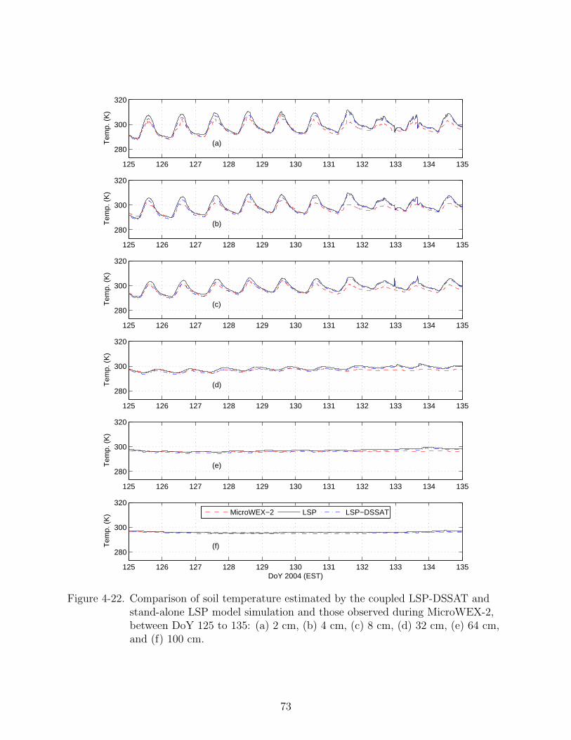
125 126 127 128 129 130 131 132 133 134 135

280

300

320

(a)Tem

p. (

K)

125 126 127 128 129 130 131 132 133 134 135

280

300

320

(b)Tem

p. (

K)

125 126 127 128 129 130 131 132 133 134 135

280

300

320

(c)Tem

p. (

K)

125 126 127 128 129 130 131 132 133 134 135

280

300

320

(d)Tem

p. (

K)

125 126 127 128 129 130 131 132 133 134 135

280

300

320

(e)Tem

p. (

K)

125 126 127 128 129 130 131 132 133 134 135

280

300

320

DoY 2004 (EST)

Tem

p. (

K)

(f)



73

135 140 145 150 155−200

0

200

400

600

800

1000

Net

Rad

iatio

n (W

/m2 )


135 140 145 150 155

−300

−200

−100

0

100

200

300

Net

Rad

iatio

n (W

/m2 )

DoY 2004 (EST)

(b)


LSP-DSSAT model simulations, the VSMs at all layers exhibit positive bias that increases

during the season. A bias of ∼0.02 m3/m3 could be introduced at the beginning of the

simulation due to improper initial conditions (Section 4.4.1) and significant uncertainty in

raingauge observations. During MicroWEX-2, the differences between daily accumulations

from the four raingauge observations and those observed independently by using

collection cans were up to 10s of mm/day. Previous studies have also found similarly

high uncertainties in precipitation, at 12 mm/h, using such raingauges [44].

The VSM bias of ∼ 0.06 m3/m3 for the layers 0.64 m and below (Figures 4-28 (e) and

(f)) could be due to the improper retention curve parameters in the clay layer (below 1.7

m). The parameters were based only on one soil sample from that layer and could have

resulted in lower flux estimates at the lower boundary and higher biases for the deeper

74

135 140 145 150 155−200

0

200

400

600

800

1000

Hea

t Flu

x (W

/m2 )

(a)


135 140 145 150 155

−300

−200

−100

0

100

200

300

Hea

t Flu

x (W

/m2 )

DoY 2004 (EST)

(b)


layers. The decrease in drainage could also cause positive bias in VSM for the upper

layers, closer to the land surface.

Overall, soil temperatures (Figure 4-29) for both model simulations match closely

with the MicroWEX-2 observations. During the bare soil period, soil temperature exhibits

positive bias of < 1.40 K and this bias is reduced during the intermediate vegetation cover

period to < 0.91 K due to a net reduction of soil heat flux estimates. As the soil heat flux

bias increases, the temperature bias increases to < 2.7 K after DoY 125. The seasonal

RMSDs decrease with depth with a maximum of 2.43 K (Table 4-6).

4.6 Conclusion

This chapter answers research questions 3, 4, and 5 given in Chapter 1.

75

135 140 145 150 1550.05

0.1

0.15

0.2 (a)V

SM

(m

3 /m3 )

135 140 145 150 1550.05

0.1

0.15

0.2 (b)

VS

M (

m3 /m

3 )

135 140 145 150 1550.05

0.1

0.15

0.2 (c)

VS

M (

m3 /m

3 )

135 140 145 150 1550.05

0.1

0.15

0.2 (d)

VS

M (

m3 /m

3 )

135 140 145 150 1550.05

0.1

0.15

0.2 (e)

VS

M (

m3 /m

3 )

135 140 145 150 1550.05

0.1

0.15

0.2 (f)

DoY 2004 (EST)

VS

M (

m3 /m

3 )



76

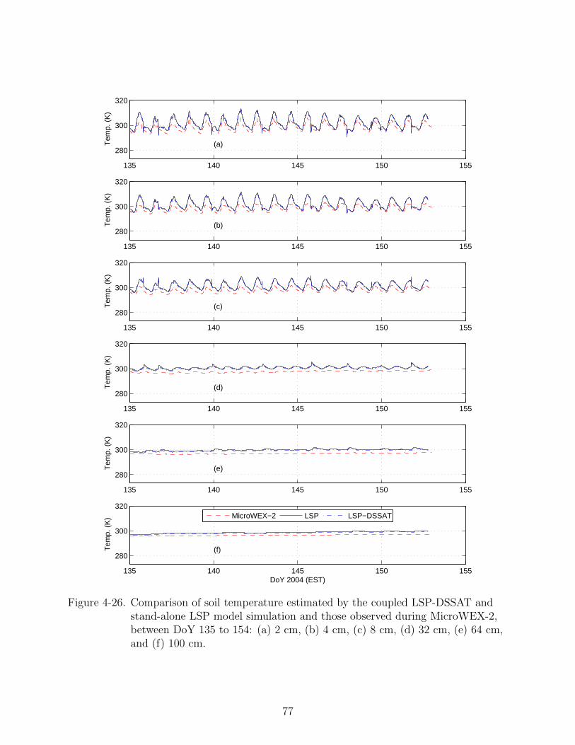
135 140 145 150 155

280

300

320

(a)Tem

p. (

K)

135 140 145 150 155

280

300

320

(b)Tem

p. (

K)

135 140 145 150 155

280

300

320

(c)Tem

p. (

K)

135 140 145 150 155

280

300

320

(d)Tem

p. (

K)

135 140 145 150 155

280

300

320

(e)Tem

p. (

K)

135 140 145 150 155

280

300

320

DoY 2004 (EST)

Tem

p. (

K)

(f)



77

80 90 100 110 120 130 140 150−200

0

200

400

600

800

1000

Flu

x (W

/m2 ) (b)

80 90 100 110 120 130 140 150

0

500

1000F

lux

(W/m

2 )

(a)

80 90 100 110 120 130 140 150−200

0

200

400

600

800

1000

Flu

x (W

/m2 ) (c)

80 90 100 110 120 130 140 150−200

0

200

400

600

800

1000

Flu

x (W

/m2 )

(d)


Figure 4-27. Comparison of fluxes estimated by the coupled LSP-DSSAT and stand-aloneLSP model simulation and those observed during MicroWEX-2: (a) netradiation, (b) latent heat flux, (c) sensible heat flux, and 2 cm soil heat flux.

78

80 90 100 110 120 130 140 1500.05

0.1

0.15

0.2(a)

VS

M (

m3 /m

3 )

80 90 100 110 120 130 140 1500.05

0.1

0.15

0.2(b)

VS

M (

m3 /m

3 )

80 90 100 110 120 130 140 1500.05

0.1

0.15

0.2(c)

VS

M (

m3 /m

3 )

80 90 100 110 120 130 140 1500.05

0.1

0.15

0.2(d)

VS

M (

m3 /m

3 )

80 90 100 110 120 130 140 1500.05

0.1

0.15

0.2(e)

VS

M (

m3 /m

3 )

80 90 100 110 120 130 140 1500.05

0.1

0.15

0.2(f)

VS

M (

m3 /m

3 )

DoY 2004 (EST)


Figure 4-28. Comparison of volumetric soil moisture estimated by the coupledLSP-DSSAT and stand-alone LSP model simulation and those observedduring MicroWEX-2: (a) 2 cm, (b) 4 cm, (c) 8 cm, (d) 32 cm, (e) 64 cm, and(f) 100 cm.

79

80 90 100 110 120 130 140 150

280

300

320

(a)Tem

p. (

K)

80 90 100 110 120 130 140 150

280

300

320

(b)Tem

p. (

K)

80 90 100 110 120 130 140 150

280

300

320

(c)Tem

p. (

K)

80 90 100 110 120 130 140 150

280

300

320

(d)Tem

p. (

K)

80 90 100 110 120 130 140 150

280

300

320

(e)Tem

p. (

K)

80 90 100 110 120 130 140 150

280

300

320

DoY 2004 (EST)

Tem

p. (

K)

(f)


Figure 4-29. Comparison of soil temperature estimated by the coupled LSP-DSSAT andstand-alone LSP model simulation and those observed during MicroWEX-2:(a) 2 cm, (b) 4 cm, (c) 8 cm, (d) 32 cm, (e) 64 cm, and (f) 100 cm.

80

Question 3:”What values of the twelve calibrated parameters give the

best LSP model performance for both latent heat flux and near surface soil

moisture for the MicroWEX-2 growing season?”

The calibrated values of the twelve parameters are given in Table 4-2.

Question 4:”How do the model estimates of soil moisture, temperature, and

surface fluxes compare with MicroWEX-2 observations?”

The RMSD for VSM at 2 cm is ∼ 0.04 m3/m3. For both the LSP and LSP-DSSAT

model simulations, the VSMs at all layers exhibit positive bias that increases during the

season. The seasonal RMSDs for temperature decrease with depth with a maximum of

2.43 K.

The RMSDs between the modeled and observed net radiation were ∼ 24 W/m2. LE

estimates had an RMSD of ∼ 48 W/m2, the sensible heat flux estimates had an RMSD of

∼ 36 W/m2, and the 2 cm soil heat flux estimates had RMSD of ∼ 47 W/m2.

Question 5:”What is the impact of coupling on both LSP and DSSAT model

estimates of LAI, biomass, soil moisture, temperature, and surface fluxes”

The estimates from the DSSAT and LSP-DSSAT differed by <0.2 for LAI and <0.6

kg/m2 for dry biomass, with the coupled LSP-DSSAT model estimating higher values than

the stand-alone DSSAT. The differences between the LSP and LSP-DSSAT estimates of

soil moisture, soil temperature, and surface fluxes are all small.

81

CHAPTER 5CANOPY MICROWAVE MODEL

5.1 Introduction

In this chapter a refractive model is developed for vegetation opacity of growing

sweet corn based upon moisture distribution in the canopy and incorporated into a

simple microwave brightness model linked with the coupled LSP-DSSAT model. The

refractive model developed by England and Galantowicz [19] was extended for sweet corn

using observed moisture distribution during the Fourth and Fifth Microwave Water and

Energy Balance Experiments (MicroWEX-4 and -5). The τ estimated by the model is

compared with that estimated using the Jackson model. The τ values obtained from the

two approximations were used in a microwave emission model at C-band and the model

estimates of brightness were compared with field observations.

5.2 Methodology

5.2.1 Moisture Distribution Measurements

Five measurements of moisture distribution were conducted during MicroWEX-4:

May 12 (Day After Planting (DAP) 63), May 17 (DAP 68), May 26 (DAP 77), June 2

(DAP 84), and June 6 (DAP 88). The samples collected on DAP 63 and 88 consisted of

plants in vegetative stage, i.e., before ear formation, while those collected on other days

consisted of plants at various reproductive stages. Additional plant sample was obtained

on DAP 88 to determine the density of wet vegetation (solid). Three measurements of

moisture distribution were conducted during MicroWEX-5: April 10 (DAP 32), May 1

(DAP 53), and May 15 (DAP 67). The samples collected on DAP 53 and 67 consisted of

plants in reproductive stages.

All representative plant samples were cut every 10 cm and weighed wet. The samples

were dried at 70o C for at least 48 hours and weighed to obtain dry biomass. The samples

on DAP 63, 2005 were cut every 5 cm to ensure that finer samples were not needed to

82

10 20 30 40 50 60 70 80 90

(a)

EarTotal

10 20 30 40 50 60 70 80 90Days After Planting

(b)

Figure 5-1. Observations of total and ear wet biomass during (a) MicroWEX-4 in 2005and (b) MicroWEX-5 in 2006.

obtain accurate moisture distribution. The density of vegetation material for each layer

was measured by volume displacement in a graduated cylinder.

Density of wet vegetation and air, ρ(z), called the cloud density, was calculated for

each layer as a ratio of wet biomass of each layer and the thickness of the layer (10 cm).

The mass of air is negligible. To obtain seasonal pattern, the cloud density of each layer

was plotted as a function of height of the layer, shown in Figure 5-3.

5.2.2 Canopy Opacity

The canopy opacity (τ) is estimated as [59, 60]:

τ =

∫ h

0

2 k0 κ(z) dz (5–1)

83

10 20 30 40 50 60 70 80 90

(a)

10 20 30 40 50 60 70 80 90

(b)

Days After Planting

Figure 5-2. Observations of canopy height during (a) MicroWEX-4 in 2005 and (b)MicroWEX-5 in 2006.

where h is canopy height (m), k0 is vacuum wavenumber (m−1), and κ(z) = −Imnt(z)(Np/m) is the absorption coefficient of the canopy. Imnt(z) is the imaginary part of the

complex refractive index, estimated as the sum of volume fraction of components,

nt(z) = 1 + vwcnwc vwc =ρ(z)

ρs

(5–2)

where, vwc is the volume fraction of the wet vegetation (m3/m3), nwc is the refractive

index of the wet vegetation , and ρs is the density of wet vegetation (697.72 kg/m3 for this

study [7]). Ulaby and El-Rayes’ model [57] estimates nwc as a function of frequency (6.7

GHz for this study) and moisture mixing ratio (Mg). Mg is defined as the ratio of weight

of water in the canopy to the weight of wet canopy. Figure 5-4 shows the mixing ratio

during MicroWEX-4 and -5. In this model, an isothermal canopy is assumed, so that the

84

κ(z) profiles can be integrated over the height of the canopy to obtain τ . The isothermal

assumption was appropriate for a short sweet corn canopy of 1.5m. The absolute difference

between the temperatures at the top and at the bottom of the canopy was < 4 K during

the simulation period.

5.2.3 Microwave Brightness Model

The microwave brightness (MB) model is a widely-used τ -ω model [59], in which the

total brightness temperature of a terrain (TB) is a sum of three contributions: TBs,p (from

the soil), TBc,p (from the canopy), and TBsky,p (from the sky).

0.2 0.4 0.6 0.8 1 1.2 1.4 1.6 1.8 2

(a)

0.2 0.4 0.6 0.8 1 1.2 1.4 1.6 1.8 2Canopy Height (m)

(b)

DAP 32DAP 53DAP 67

DAP 63DAP 68DAP 77DAP 84DAP 88

Figure 5-3. Cloud densities measured during (a) MicroWEX-4 in 2005 and (b)MicroWEX-5 in 2006. The symbols and the lines represent the measurementsand the best curve-fits, respectively.

85

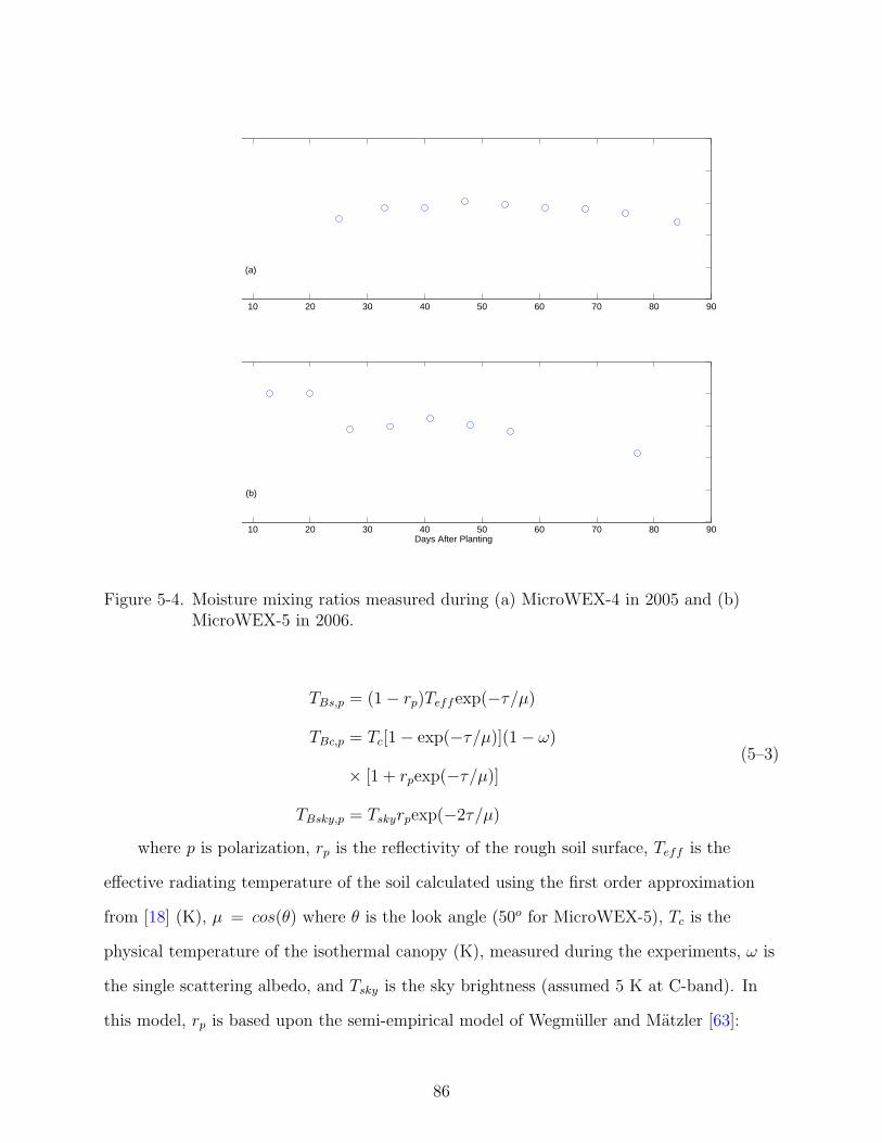
10 20 30 40 50 60 70 80 90

(a)

10 20 30 40 50 60 70 80 90

(b)

Days After Planting

Figure 5-4. Moisture mixing ratios measured during (a) MicroWEX-4 in 2005 and (b)MicroWEX-5 in 2006.

TBs,p = (1− rp)Teffexp(−τ/µ)

TBc,p = Tc[1− exp(−τ/µ)](1− ω)

× [1 + rpexp(−τ/µ)]

TBsky,p = Tskyrpexp(−2τ/µ)

(5–3)

where p is polarization, rp is the reflectivity of the rough soil surface, Teff is the

effective radiating temperature of the soil calculated using the first order approximation

from [18] (K), µ = cos(θ) where θ is the look angle (50o for MicroWEX-5), Tc is the

physical temperature of the isothermal canopy (K), measured during the experiments, ω is

the single scattering albedo, and Tsky is the sky brightness (assumed 5 K at C-band). In

this model, rp is based upon the semi-empirical model of Wegmuller and Matzler [63]:

86

rH = |ΓH |2e−(k0σ)√

0.1cos(θ)

rV = rHcos(θ)0.655

(5–4)

where ΓH is the H-polarized Fresnel coefficient, k0 is the vacuum wavenumber, θ is

the look angle, and σ is the surface roughness height, set to 0.0005 m [27]. Soil dielectric

properties are determined using a four component mixing model following Dobson et al

[13].

5.2.4 Model Comparison and Evaluation

Using the ρ(z), τ is obtained for the MicroWEX-4 and -5 growing seasons. The

estimates for τ are compared with those obtained using the Jackson model [51] as:

τ = bWc (5–5)

where, b is an empirical parameter and Wc is the water content in the canopy (kg/m2).

The τ from the biophysical model and from the Jackson model are evaluated in the

MB model during the latter part of the MicroWEX-5 season. The MB model simulated

TB for ten days (DAP 42-52), with DAP 42-47 during vegetative growth and DAP 47-52

during ear formation. The canopy cover was 100% during the period of simulation. The

MB model was driven with observed canopy and soil temperatures and moisture values.

The MB model was linked to the LSP-DSSAT model, which provides it with soil

temperature and moisture profiles as well as canopy properties used for calculating canopy

transmission and scattering, such as height, vegetation cover, and vegetative and ear

biomass. Using the same initial conditions, inputs, and parameters obtained for the

calibrated LSP-DSSAT model in Chapter 4, the LSP-DSSAT-MB model simulated H-pol

TB for the MicroWEX-2 growing season.

87

Table 5-1. Values of the Coefficients in equations 5–6 and 5–7

Coefficients Valuesa 2.054b -2.054αc -114.32αd 5.87αe -1.23βc 25.69βd -1.37βe 0.34γc 8.41γd 0.29γe -0.07


5.3.1 Moisture Distribution Function

As shown in Figure 5-3, the cloud density function consists of two terms, a linear

term representing the vegetative stage of the plant and a gaussian term representing the

moisture in the ear during the reproductive stages, as:

ρ(z) =Bv

h(a+ bhn) + c

Be

hexp

[−1

2

(hn − d

e

)2](5–6)

where a, b, c, d, and e are fitted parameters, hn = z/h is the normalized height, and Bv

and Be are the wet biomass of vegetation (stem and leaves) and ear (kg/m2), respectively.

Figure 5-3 also shows the best curve-fits obtained for each sample. The parameters c, d,

and e, governing the gaussian term, were estimated as quadratic functions of dry biomass

of the ear (Dear) as:

c = αc + βcDear + γcD2ear

d = αd + βdDear + γdD2ear

e = αe + βeDear + γeD2ear

(5–7)

Table 5-1 gives the values of the a and b parameters and the coefficients in equation 5–7.

88

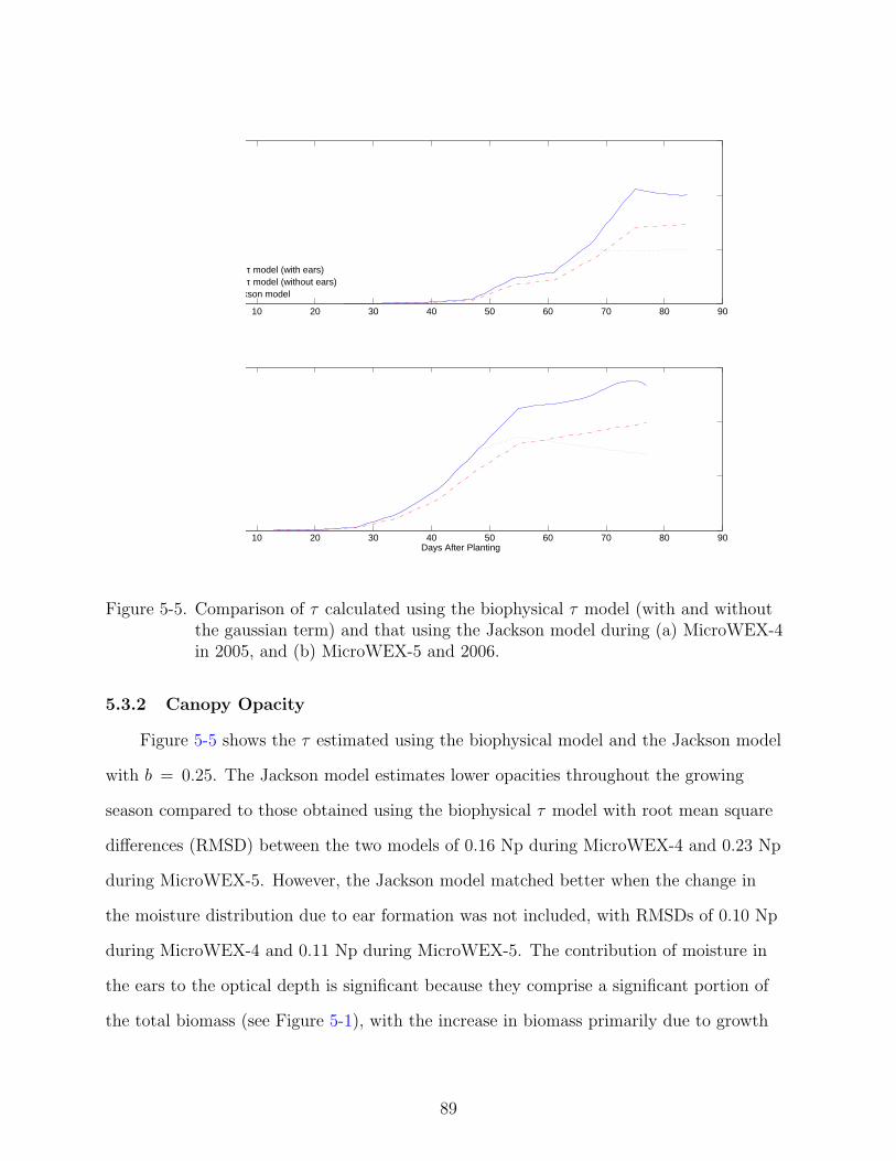
10 20 30 40 50 60 70 80 90

10 20 30 40 50 60 70 80 90Days After Planting

Our τ model (with ears)Our τ model (without ears)Jackson model

Figure 5-5. Comparison of τ calculated using the biophysical τ model (with and withoutthe gaussian term) and that using the Jackson model during (a) MicroWEX-4in 2005, and (b) MicroWEX-5 and 2006.

5.3.2 Canopy Opacity

Figure 5-5 shows the τ estimated using the biophysical model and the Jackson model

with b = 0.25. The Jackson model estimates lower opacities throughout the growing

season compared to those obtained using the biophysical τ model with root mean square

differences (RMSD) between the two models of 0.16 Np during MicroWEX-4 and 0.23 Np

during MicroWEX-5. However, the Jackson model matched better when the change in

the moisture distribution due to ear formation was not included, with RMSDs of 0.10 Np

during MicroWEX-4 and 0.11 Np during MicroWEX-5. The contribution of moisture in

the ears to the optical depth is significant because they comprise a significant portion of

the total biomass (see Figure 5-1), with the increase in biomass primarily due to growth

89

in ears once corn reaches the reproductive stage. As a result, Figure 5-5 shows a sharp

increase in optical depth at the onset of ear development, at DAP 62 for MicroWEX-4 and

DAP 47 for MicroWEX-5. By the end of the seasons, the optical depth is doubled when

ears are included.

5.3.3 Microwave Brightness

Figure 5-6 shows the comparison of the horizontally polarized (H-pol) TB observed

during MicroWEX-5 with those simulated by the MB model at C-band, with τ estimates

using the biophysical model and the Jackson model. Only H-pol brightness is examined

here because H-pol brightness is more sensitive to changes in soil moisture than V-pol, at

the incidence angle of 50o, that is close to the Brewster angle at microwave frequencies

[59]. The observed TB increased during the drydown from DAP 42 to DAP 46.7 and then

43 44 45 46 47 48 49 50 51 52Days After Planting (EST)

MB model (our τ)MB model (Jackson τ)MicroWEX−5 Observations

Figure 5-6. Comparison of the observed TB at H-pol during MW5 those simulated by theMB model using τ from the biophysical model and from the Jackson modelduring late-season MicroWEX-5.

90

Table 5-2. RMS differences between observed TB during MicroWEX-5 and those estimatedby the MB model

RMSD (K)τ model DAP < 47 DAP ≥ 47 DAP 42-52

Jackson (ω = 0.00) 5.84 12.50 9.74Jackson (ω = 0.06 for DAP ≥ 47) 5.84 3.65 4.88

Biophysical ω = 0.05 for 42<DAP<52 5.00 8.25 6.83Biophysical ω = 0.075 for DAP ≥ 47 5.00 5.22 5.13

decreased by 30 K due to an irrigation event. The TB at 6.7 GHz were sensitive to soil

moisture changes even when the canopy cover was 100% and biomass was 2.7 kg/m2 (see

Figure 5-1).

A small value for single-scattering albedo (ω) was included in the MB model when

using the biophysical τ estimates. The value of 0.05 before ear formation (DAP 47) and

0.075 after DAP 47 provided the least RMSD (see Table 5-2).

In the Jackson model, b = 0.25, similar to the literature-based values for corn [61],

provided the lowest RMSD. Typically ω is set to zero in the Jackson model [51], but it was

found that the TB using the Jackson model was overestimated after ear formation, with an

RMSD of 12.50 K. Including ω = 0.06 after ear formation in the Jackson model reduced

the RMSD to 3.65 K,as shown in Table 5-2. The values of ω needed to provide the least

RMSD for both τ models were small, < 0.1, implying that single scattering is sufficient to

provide realistic TB estimates for the mature sweet corn canopy and multiple scattering is

not needed. The overall RMSD between observed TB and the modeled TB using the two

τ models were similar, with 5.13 K for the biophysical model and 4.88 K for the Jackson

model (see Table 5-2).

91

8085

9095

100

105

110

115

120

125

140

160

180

200

220

240

260

280

300

320

H−pol Brightness Temp. (K)

(a)

8085

9095

100

105

110

115

120

125

140

160

180

200

220

240

260

280

300

320


(b)

DoY

200

4 (E

ST

)

M

icro

WE

X−

2LS

P−

DS

SA

T−

MB

Fig

ure

5-7.

Com

par

ison

ofm

icro

wav

ebri

ghtn

ess,

esti

mat

edby

the

LSP

-DSSA

T-M

Bm

odel

wit

hsp

ecula

rsu

rfac

e(a

)an

dW

egm

uller

and

Mat

zler

(b),

and

C-b

and

mic

row

ave

bri

ghtn

ess

obse

rved

duri

ng

Mic

roW

EX

-2,bef

ore

DoY

125.

92

125

130

135

140

145

150

155

180

200

220

240

260

280

300

320


(a)

125

130

135

140

145

150

155

180

200

220

240

260

280

300

320


(b)

DoY

200

4 (E

ST

)

Mic

roW

EX

−2

LSP

−D

SS

AT

−M

B

Fig

ure

5-8.

Com

par

ison

ofm

icro

wav

ebri

ghtn

ess,

esti

mat

edby

the

LSP

-DSSA

T-M

Bm

odel

wit

hsp

ecula

rsu

rfac

e(a

)an

dW

egm

uller

and

Mat

zler

(b),

and

C-b

and

mic

row

ave

bri

ghtn

ess

obse

rved

duri

ng

Mic

roW

EX

-2,af

ter

DoY

125.

93

Table 5-3. RMS differences between observed H-pol TB during MicroWEX-2 and thoseestimated by the MB model.

rp model RMSD (K) MAD (K) Bias (K)Specular soil (DoY < 125) 35.87 28.94 -25.70

Wegmuller and Matzler (DoY < 125) 32.18 23.78 14.43Specular soil (DoY ≥ 125) 10.06 8.15 6.58

Wegmuller and Matzler (DoY ≥ 125) 12.43 10.83 9.97

During less than full vegetation cover (before DoY 125), the soil reflectivity strongly

affects the estimation of brightness. This leads to a wide disparity between the specular

and Wegmuller and Matzler rough surface model estimates, as can be seen in Figure 5-7.

The lower reflectivity of the rough surface model leads to higher brightness values than

the specular model. Sudden drops in brightness (DoY 98, 100, 104, 107, 109, 112, 114,

119, 122, 123, and 124) due to irrigation or precipitation events are only reached with

the specular model. As vegetation cover increases, the canopy contribution to brightness

increases so the specular and rough surface models’ estimates of brightness approach

eachother. Overall, the performance when vc < 1 is poor, as seen by the high RMSDs

Table 5-3. Neither reflectivity model matched sudden drops in brightness, and there is also

an underestimation due to the overestimation of soil moisture by the LSP model (Chapter

4).

During full vegetation cover (after DoY 125), model estimates of brightness are

dominated by the canopy contribution and thus by τ and ω. Both surface reflectivity

models give similar results and overestimate brightness, seen in Figure 5-8 and the RMSDs

in Table 5-3. This could be an indication that the ω values found for MicroWEX-5 are

not correct for MicroWEX-2. After modeled ear formation on DoY 139 brightness is less

overestimated as ω is increased to 0.075. This late in the season, there is almost no effect

from the soil, and as the τ model is biophysically based, the only way to improve model

estimates here would be to calibrate ω before and after ear formation.

5.4 Summary

This chapter answers the research question 6 and 7 outlined in Chapter 1.

94

Question 6:”How does a physically-based τ model compare to Jackson’s

widely-used empirical model?”.

The τ obtained from the biophysical model estimated higher values than the Jackson,

with an RMSD between the two of up to 0.23 Np. The τ values obtained from the two

approximations were used in a microwave emission model at C-band, the model estimates

of TB matched well with observations using both τ values when ω is included, with similar

RMSDs of ∼ 5 K.

Question 7:”How do the brightness estimates predicted by the linked LSP-

DSSAT-MB model compare to observations during MicroWEX-2?”

Preliminary results indicate the MB model is lacking in two main areas, the roughness

model and the ω model. For the first half of the season, where bare soil brightness is more

important, the constant roughness or specular surface models over- and under-estimate

brightness, respectively, both with RMSDs ∼ 33 K. During the later half of MicroWEX-2,

brightness is overestimated with RMSD of ∼ 11 K.

95

CHAPTER 6CONCLUSION

In this chapter, the results and contributions from this thesis are summarized and

reccomendations for future research are provided.

6.1 Summary

This thesis provides important insights into crop, SVAT, and microwave brightness

modeling for growing vegetation. Three season-long extensive field experiments (MicroWEX-2,

4, and 5) were conducted, monitoring radiobrightness, soil moisture, soil temperature,

surface fluxes, and crop growth for sweet corn. These experiments provided the datasets

used in forcing, developing, and calibrating the models.

First, a crop model and SVAT model were calibrated and coupled. The crop model

(CERES-Maize) was calibrated with simulated annealing using field observations for the

MicroWEX-2 site. The calibration was performed by minimizing the residuals for LAI

and biomass, the two most important canopy parameters in determining the microwave

signature of a vegetation canopy. The SVAT model (LSP) was calibrated with Latin

Hypercube Sampling to provide the least RMSD in LE with an RMSD in VSM at 2 cm of

∼0.04 m3/m3, using observations during MicroWEX-2. The LSP and DSSAT models were

coupled such that the LSP replaced the DSSAT soil and soil-plant-atmosphere modules

while DSSAT provides LSP with LAI, biomass, height, width, and root length density.

Model estimates of surface fluxes, VSM, and soil temperature were very similar using both

the coupled LSP-DSSAT and stand-alone LSP that used observed vegetation parameters.

Second, a microwave transmission model was developed and compared with the

widely-used empirical Jackson model, and with observations of of microwave brightness

for a period during MicroWEX-5. This τ model was incorporated in a MB linked with

the coupled LSP-DSSAT model, and tested for the MicroWEX-2 growing season.

The τ obtained from the biophysical model estimated higher values than the Jackson,

with an RMSD between the two of up to 0.23 Np. The τ values obtained from the two

96

approximations were used in a microwave emission model at C-band, the model estimates

of TB matched well with observations during MicroWEX-5, using both τ values when ω is

included, with similar RMSDs.

The brightness temperatures predicted by the linked LSP-DSSAT-MB model

during the first half of the MicroWEX-2tested for MicroWEX-2, for the first half of

the MicroWEX-2 season were higher than those observed when the Wegmuller and

Matzler reflectivity model was used and were significantly lower than observations when

a specular model was used. In addition, overestimation of moisture by the LSP model

lead to underestimation of brightness. Later in the MicroWEX-2 season, brightness is

overestimated when using the ω values found for MicroWEX-5, suggesting they are too

low.

6.2 Contributions

One of the major contributions of this thesis is the development and calibration of

the coupled SVAT-Crop model as well as the development of the physically-based canopy

transmission model for sweet corn. The techniques used to couple the LSP and DSSAT

models can be extended to other SVAT-Crop combinations; likewise, the methodology for

developing the optical depth model for sweet corn can be extended to other plant types, as

has been done for cotton during MicroWEX-6 [67].

Other significant contributions are the extensive datasets of soil temperature, soil

moisture, vegetation, surface fluxes, and radiobrightness collected during MicroWEX-2,

4, and 5. They provide season-long and high temporal resolution observations to allow

interdisciplinary studies.

6.3 Recommendations for Future Research

As seen in Chapter 4, the LSP-DSSAT model overestimates soil moisture, largely

due to uncertainty in soil hydrologic properties and in precipitation. This indicates that

the model estimates would improve with a calibration of the soil hydrologic parameters

in addition to the twelve parameters calibrated in Chapter 4. In addition, since a major

97

source of uncertainty in the model is the precipitation input, model estimates of soil

moisture are likely to improve from a data assimilation method which takes into account

the uncertainty in inputs and parameters, such as Kalman filtering.

Before the LSP-DSSAT-MB model can be used in a data assimilation scheme, the

rough soil reflectivity model in the MB model needs to be improved. As is shown in

Section 5.3.3, from the high brightness RMSDs during the first half of the season, either

the specular (Fresnel) reflectivity or the rough surface reflectivity alone are insufficient

to match the sudden drops in brightness associated with precipitation events. This is a

challenge because of the extremely limited bare soil brightness data during MicroWEXs

2, 4, and 5. To fill the dearth of bare soil data, bare soil tests were conducted during

May and June 2007 in which extensive soil roughness measurements were taken along

with brightness measurements, before, during, and after irrigation events. This data

would be useful in the future for the development of a more rigorous rough surface

reflectivity model. A moisture-dependent roughness model could capture the sudden drops

in brightness associated with precipitation events but needs to be refined.

In addition, the LSP-DSSAT-MB model overestimated brightness in the later

half of the MicroWEX-2 season, indicating that the ω values need to be higher for the

MicroWEX-2, and that they should be calibrated. The optimal ω values for MicroWEX-2

and MicroWEX-5 are apparently different, indicating that there is some difference between

the canopies of the two seasons that would produce a difference in ω. Future research

could find some physical relationship between canopy characteristics such as leaf or stem

biomass and ω, similar to the physical relationship found for τ .

98

REFERENCES

[1] Boland, J., L. Scott, and M. Luther (2001), Modelling the diffuse fraction of globalsolar radiation on a horizontal surface, Environmetrics, 12, 103–116.

[2] Busetti, F. (2004), Simulated annealing overview, Tech. rep., Available atwww.geocities.com/francorbusetti/saweb.pdf.

[3] Camillo, P., and R. J. Gurney (1986), A resistance parameter for bare soilevaporation models, Soil Science, 141, 95–105.

[4] Campbell, G. S., and J. M. Norman (1998), An Introduction to EnvironmentalBiophysics, 2nd ed., 286 pp., Springer Science+Business Media, New York.

[5] Campbell Scientific (2006), CS616 and CS625 Water Content Reflectometers, Tech.rep., Available at http://www.campbellsci.com/documents/manuals/cs616.pdf,Logan, Utah.

[6] Casanova, J., T. Lin, M. Jang, K. Tien, J. Judge, O. Lanni, and L. Miller (2005),Field observations during the fourth microwave water and energy balance experiment(MicroWEX-4): From March 10-June 14, 2005, Tech. Rep. Circular No 1482, Centerfor Remote Sensing, University of Florida, Available at UF/IFAS EDIS website athttp://edis.ifas.ufl.edu/AE362.

[7] Casanova, J., M. Jang, and J. Judge (2006), Vertical distribution of moisturein a sweet corn canopy, Tech. Rep. Circular No 1492, Center for RemoteSensing, University of Florida, Available at UF/IFAS EDIS website athttp://edis.ifas.ufl.edu/AE395.

[8] Casanova, J., F. Yan, K. Tien, J. Judge, O. Lanni, and L. Miller (2006), Fieldobservations during the fifth microwave water and energy balance experiment(MicroWEX-5): From march 9-may 26, 2006, Tech. Rep. Circular No 1514, Centerfor Remote Sensing, University of Florida, Available at UF/IFAS EDIS website athttp://edis.ifas.ufl.edu/AE407.

[9] Chung, Y. (2007), A snow-soil-vegetation-atmosphere-transfer/radiobrightness modelfor wet snow, Ph.D. thesis, University of Michigan.

[10] Dai, Y., et al. (2003), The Common Land Model (CLM), Bull. Amer. Meteor Soc.,84(8), 1013–1023.

[11] de Vries, D. A. (1963), Thermal properties of soils, in Physics of Plant Environ-ment, edited by W. R. van Wijk, North-Holland Publishing Company, Amsterdam,Netherlands.

[12] Demarty, J., C. Ottle, I. Braud, and J. Frangi (2002), Comparison of measured andSISPAT-RS simulated brightness temperatures and reflectances at field scale duringReSeDA experiment, Proceedings of SPIE, the International Society for Optical

99

EngineeringProceedings of SPIE, the International Society for Optical Engineering,4542.

[13] Dobson, M., F. Ulaby, M. Hallikainen, and M. El-Rayes (1985), Microwave dielectricbehavior of wet soil-part II: Dielectric mixing models, IEEE Trans. Geosci. RemoteSensing, GE-23, 35–46.

[14] Doorenbos, J., and W. Pruitt (1977), Guidelines for predicting crop waterrequirements, Tech. Rep. Irrigation and drainage paper No. 24, United NationsFAO.

[15] Du, Y., F. Ulaby, and M. Dobson (2000), Sensitivity to soil moisture by active andpassive microwave sensors, IEEE Trans. Geosci. Remote Sensing, 38 (1), 105–114.

[16] Dukes, M. (2004), Update of the AFSIRS crop water use simulation model.Micrometeorological dataset, Tech. rep., Available at http://afsirs.ifas.edu.

[17] Dyer, A. J. N. (1974), A review of flux-profile relationships, Boundary-Layer Meteo-rology, 7(3), 363–372.

[18] England, A. (1990), Radiobrightness of diurnally heated, freezing soil, IEEE Trans.Geosci. Remote Sensing, 28 (4), 464–76.

[19] England, A., and J. Galantowicz (1995), Moisture in a grass canopy from SSM/Iradiobrightness, in Proc. 2nd Tropical Symposium on Combined Optical-MicrowaveEarth and Atmos. Sensing, vol. Atlanta, GA, pp. 12–14.

[20] Enthekabi, D., et al. (2004), The Hydrosphere (HYDROS) Satellite Mission: an Earthsystem pathfinder for global mapping of soil moisture and land freeze thaw, IEEETransactions on Geoscience and Remote Sensing, 42(10), 2184–2195.

[21] Eom, H.J. (1992), A thermal microwave emission model for row-structured vegetation,Int. J. Remote Sensing, 13 (16), 2975–2982.

[22] EOS (2003), Advanced microwave scanning radiometer for eos, overview, sensor, andorbit, Tech. rep., Available at http://www.ghcc.msfc.nasa.gov-/AMSR/.

[23] Garcia-Quijano, J. F., and A. P. Barros (2005), Incorporating physiology into ahydrological model: photosynthesis, dynamic respiration, and stomatal sensitivity,Ecological Modeling, 185, 29–49.

[24] Goudriaan, J. (1977), Crop Micrometeorology: A Simulation Study, 1st ed., 249 pp.,Centre for Agricultural Publishing and Documentation, Wageningen, the Netherlands.

[25] Gupta, H. V., L. A. Bastidas, S. Sorooshian, W. J. Shuttleworth, and Z. L. Yang(1999), Parameter estimation of a land surface scheme using multicriteria methods,Journal of Geophysical Research, 104(D16), 19,491–19,503.

100

[26] Jackson, T., and T. Schmugge (1989), Passive microwave remote sensing system forsoil moisture: Some supporting research, IEEE Trans. Geosci. Remote Sensing, 27 (2),225–235.

[27] Jang, M.Y., K. Tien, J.Casanova, and J.Judge (2005), Measurements of soilsurface roughness during during the fourth microwave water and energy balanceexperiment: From April 18-June 13, 2005, Tech. Rep. Circular No 1483, Centerfor Remote Sensing, University of Florida, Available at UF/IFAS EDIS website athttp://edis.ifas.ufl.edu/AE393.

[28] Jones, C., and J. Kiniry (Eds.) (1986), CERES-Maize: A Simulation Model of MaizeGrowth and Development, Texas A&M University Press, College Station, Texas.

[29] Jones, J. W., G. Hoogenboom, C. Porter, K. Boote, W. B. L. Hunt, P. Wilkens,U. Singh, A. Gijsman, and J. Ritchie (2003), The DSSAT cropping system model,European J. Agronomy, 18(3-4), 235–265.

[30] Judge, J., A. England, C. L. W. Crosson, B. Hornbuckle, D. Boprie, E. Kim, andY. Liou (1999), A growing season land surface process/radiobrightness model forwheat-stubble in the southern great plains, IEEE Trans. Geosci. Remote Sensing,37 (5), 2152–2158.

[31] Judge, J., L. Abriola, and A. England (2003), Development and numerical validationof a summertime land surface processand radiobrightness model, Advances in WaterResources, 26(7), 733–746.

[32] Judge, J., A. W. England, J. R. Metcalfe, D. McNichol, and B. E. Goodison (2007),Calibration of an integrated land surface process and radiobrightness (LSP/R) modelduring summertime, Advances in Water Resources, In Press.

[33] Judge, Jasmeet, J. Casanove, T. Lin, K. Tien, M. Jang, J. Judge, O. Lanni, andL. Miller (2004), Field observations during the second microwave water and energybalance experiment (MicroWEX-2): From March 17-June 3, 2004, Tech. Rep.Circular No 1480, Center for Remote Sensing, University of Florida, Available atUF/IFAS EDIS website at http://edis.ifas.ufl.edu/AE360.

[34] Kerr, Y. H., P. Waldteufel, J. Wigneron, J. Martinuzzi, J. Font, and M. Berger (),Soil moisture retrieval from space: the Soil Moisture and Ocean Salinity (SMOS)mission, IEEE Transactions on Geoscience and Remote Sensing, 39.

[35] Kustas, W. P., and J. M. Norman (2000), A two-source energy balance approachusing directional radiometric temperature observations for sparse canopy coveredsurfaces, Agron. J., 92, 847–854.

[36] Leese, J., T. Jackson, A. Pitman, and P. Dirmeyer (2001), GEWEX/BAHCinternational workshop on soil moisture monitoring, analysis, and prediction forhydrometeorological and hydroclimatological applications, Bull. Amer. Meteorol. Soc.,82(7), 1423–1430.

101

[37] Lin, Tzu-yun, J. Judge, K. Tien, , J. C. andM.Y. Jang, O. Lanni, and L. Miller(2004), Field observations during the third microwave water and energy balanceexperiment (MicroWEX-3): From july 16-december 21, 2004, Tech. Rep. Circular No1483, Center for Remote Sensing, University of Florida, Available at UF/IFAS EDISwebsite at http://edis.ifas.ufl.edu/AE361.

[38] Liou, Y., J. Galantowicz, and A. England (1998), A land surfaceprocess/radiobrightness model with coupled heat and moisture transport for freezingsoils, IEEE Trans. Geosci. Remote Sennsong, 36(2), 669–677.

[39] Manabe, S. (1969), Climate and the ocean circulation. 1. The atmosphere circulationand the hydrology of the earth’s surface, Month. Weat. Rev., 97 (11), 739–774.

[40] McKay, M. D., R. J. Beckman, and W. J. Conover (2000), A comparison of threemethods for selecting values of input variables in the ananlysis of output from acomputer code, Technometrics, 42(1), 55–61.

[41] Mo, X., S. Liu, Z. Lin, Y. Xu, Y. Xiang, and T. McVicar (2005), Prediction of cropyield, water consumption and water use efficiency with a svat-crop growth modelusing remotely sensed data from the North China plain, Ecological Modelling, 183,301–322.

[42] Niu, G.-Y., and Z.-L. Yang (2004), Effects of vegetation canopy processes on snowsurface energy and mass balances, J. Geophys. Res., 109, D23,111, doi:10.1029/2004JD004884.

[43] Njoku, E.G., and J. Kong (1977), Theory for passive microwave remote sensing ofnear-surface soil moisture, J. Geophys. Res., 82 (20), 3108–18.

[44] Nyusten, J. A., J. R. Front, P. G. Black, and J. C. Wilkerson (1996), A comparison ofautomatic rain gauges, Journal of Atmospheric and Oceanic Technology, 13(1), 62–73.

[45] Omega (2006), Thermistor elements and compatibleinstrumentation, Tech. rep., Available athttp://www.omega.com/Temperature/pdf/44000 THERMIS ELEMENTS.pdf.

[46] Pan, H.-L., and L. Mahrt (1987), Interaction between soil hydrology and boundarylayer development, Boundary Layer Meteorology, 38, 185–202.

[47] Philip, J. R., and D. A. de Vries (1957), Moisture movement in porous material undertemperature gradients, Transactions of American Geophysical Union, 38, 222–232.

[48] Ritchie, J. (1972), Model for predicting evaporation from a row crop with incompletecover, Water Resources Res., 8, 1204–1213.

[49] Rossi, C., and J. R. Nimmo (1994), Modeling of soil water retention from saturationto oven dryness, Water Resources Research, 30, 701–708.

102

[50] Sau, F., K. Boote, W. M. Bostick, J. Jones, , and M. I. Minguez (2004), Testing andimproving evapotranspiration and soil water balance of the DSSAT crop models,Agronomy J., 96 (5), 1243–1257.

[51] Schmugge, T., and T. Jackson (1992), A dielectric model of the vegetation effectson the microwave emission from soils, IEEE Trans. Geosci. Remote Sensing, 30 (4),757–760.

[52] Schmugge, T., and P. O’Neill (1986), Passive microwave soil moisture research, IEEETrans. Geosci. Remote Sensing, GE-24 (1), 12–22.

[53] Soil Conservation Service (1972), National engineering handbook: Section 4:Hydrology, Tech. rep., USDA.

[54] Thornley, J., and I. Johnson (1990), Plant and Crop Modeling., Oxford: OxfordUniversity Press.

[55] Tien, Kai-Jen, J. Judge, O. Lanni, and L. Miller (2003), Field observations duringthe second microwave water and energy balance experiment (MicroWEX-1):From July 17 - December 16, 2003, Tech. Rep. Circular No 1470, Center forRemote Sensing, University of Florida, Available at UF/IFAS EDIS website athttp://edis.ifas.ufl.edu/AE280.

[56] Twine, T., W. P. Kustas, J. M. Norman, D. R. Cook, P. R. Houser, T. P. Meyers,J. H. Prueger, P. J. Starks, and M. L. Wesely (2000), Correcting eddy-covariance fluxunderestimates over a grassland, Agricultural and Forest Meteorology, 103, 279–300.

[57] Ulaby, F., and M. El-Rayes (1987), Microwave dielectric spectrum ofvegetation-PartII: Dual- dispersion model, IEEE Trans. Geosci. Remote Sensing,GE-25, 550–557.

[58] Ulaby, F., and E. Wilson (1985), Microwave attenuation properties of vegetationcanopies, IEEE Trans. Geosci. Remote Sensing, GE-23, 746–753.

[59] Ulaby, F., R. Moore, and A. Fung (1981), Microwave Remote Sensing Active andPassive, Vol I, Artech House Inc.: Norwood, MA.

[60] Ulaby, F., R. Moore, and A. Fung (1986), Microwave Remote Sensing Active andPassive, Vol III, Artech House Inc.: Norwood, MA.

[61] Van de Griend, A. A., and J. Wigneron (2004), The b-factor as a function offrequency and canopy type at H-polarization, IEEE Trans. Geosci. Remote Sens-ing, 42 (4), 786–794.

[62] Verseghy, D. L., N. A. McFarlane, and M. Lazare (1993), Class - a Canadian landsurface scheme for GCMs II. Vegetation model and coupled runs, Int. J. of Climatol-ogy, 13, 347–370.

103

[63] Wegmuller, U., and C. Matzler (1999), Rough bare soil reflectivity model, IEEETrans. Geosci. Remote Sensing, 37 (3), 1391–1396.

[64] Whitfield, B., J. Jacobs, and J. Judge (2006), Intercomparison study of the landsurface process model and the common land model for a prairie wetland in Florida,Journal of Hydrometeorology, 7(6), 1247–1258.

[65] Williams, J., P. Dyke, and C. Jones (1983), EPIC: A model for assessing the effects oferosion on soil productivity, Elsevier, Amsterdam.

[66] Willmott, C. J. (1982), Some comments on the evaluation of model performance,Bulletin of the American Meteorological Society, 63, 1309–1313.

[67] Yan, Fei, J. Casanova, K. Tien, J. Judge, O. Lanni, and L. Miller (2006), Fieldobservations during the sixth microwave water and energy balance experiment(MicroWEX-6): From June 19-October 31, 2006, Tech. Rep. Circular No 1515,Center for Remote Sensing, University of Florida, Available at UF/IFAS EDISwebsite at http://edis.ifas.ufl.edu/AE409.

104

BIOGRAPHICAL SKETCH

Joaquin Casanova was born on December 25, 1984, in Gainesville, Florida. Some stuff

happened, then in 2006 he got his BS in Agricultural and Biological Engineering from UF.

105

modeling land surface fluxes and...

Documents