modeling electricity trade in southern africa user manual for
TRANSCRIPT

Modeling Electricity Trade in Southern AfricaUSER MANUAL
FOR THELONG-TERM MODEL
African Economic ResearchResearch Report
Second Edition, January 1999
F. T. Sparrow and Brian H. BowenPurdue University
Funded byUnited States Agency for International Development
Bureau for AfricaOffice of Sustainable Development
Washington, DC 20523-4600
The views and interpretations in this peaper are those of the authorsand not necessarily of the affiliated institutions.

i
User Manual
TABLE OF CONTENTS
List of Tables............................................................................................................................iii
ACKNOWLEDGEMENTS..................................................................................................... iv
NOTATION ..............................................................................................................................v
Chapter 1: Background to the User Manual ..........................................................................1
Chapter 2: The Long-Run Model in Simple, Modular Form............................................... 11
2.1 Introduction................................................................................................................................................. 11
2.2 Overview of the Model Use.......................................................................................................................... 13
2.3 The Model in Simple Modular Form.................................................................................................... 21
2.4 The Supply - Demand Module.............................................................................................................. 21
2.5 The Capacity Constraint Module......................................................................................................... 222.5.1. Generation .................................................................................................................................... 222.5.2 Transmission................................................................................................................................. 26
2.6 The Reliability Module ......................................................................................................................... 26
2.7 The Country Autonomy Module .......................................................................................................... 28
2.8 The Objective Function Module........................................................................................................... 282.8.1. Operating Costs............................................................................................................................. 292.8.2 New Equipment Costs ................................................................................................................... 29
2.9 Summary of the Model ......................................................................................................................... 312.9.1 The Demand/Supply Module ......................................................................................................... 312.9.2 The Capacity Constraint Module.................................................................................................... 312.9.3 The Reliability Module.................................................................................................................. 33
2.10 The Country Autonomy Module...................................................................................................... 34
2.11 The Objective Function Module ...................................................................................................... 35
Chapter 3: Operating Instructions........................................................................................ 37
3.1 Computing Requirements and Setting of Parameters ................................................................................ 42
3.2 Power Supply from New and Old Thermal Sites ........................................................................................ 46

ii
3.3 Power Supply from New and Old Hydropower Sites.................................................................................. 47
3.4 Transmission and Trade.............................................................................................................................. 48
3.5 Demand and Reliability............................................................................................................................... 49
3.6 Finances ....................................................................................................................................................... 50
3.7 Output Files ................................................................................................................................................. 55
3.8 Questions Related to The Formulation ....................................................................................................... 56
Chapter 4: The Full Long-Run Model .................................................................................. 63
4.1 The Demand/Supply Equations............................................................................................................ 634.1.1 The Demand for Electricity............................................................................................................ 634.1.2 The Supply Side ............................................................................................................................ 714.1.3 The Full System Load Balance Equation........................................................................................ 76
4.2 The Capacity Constraint Module......................................................................................................... 774.2.1 Old Thermal Sites.......................................................................................................................... 794.2.2 Old Hydro Sites............................................................................................................................. 844.2.3 New Thermal Plants ...................................................................................................................... 874.2.5 Large Combined Cycle and Large Coal Plants ............................................................................... 934.2.6 The Treatment of SAPP approved New Thermal Plants................................................................ 1004.2.7 New Hydro Capacity Constraints................................................................................................. 1034.2.8 Old Transmission Lines............................................................................................................... 1064.2.9 New Transmission Lines ............................................................................................................. 1084.2.10 Pumped Storage Capacity Constraints.......................................................................................... 110
4.3 The Reliability Constraints ................................................................................................................ 1134.3.1 The Autonomy Constraint............................................................................................................ 117
4.4 The Objective Function Module......................................................................................................... 1184.4.1 Fuel and Operating Costs............................................................................................................. 1184.4.2 Cost of Unserved Energy ............................................................................................................. 1204.4.3 Capital Cost ................................................................................................................................ 1204.4.4 Final Expression of the Objective Function.................................................................................. 1274.4.5 The Budget Constraint................................................................................................................. 128
List of FiguresFigure 1.1 Republic of South Africa’s Demand (MW), July 24, 1997 ..................................................................... 4Figure 1.2 Demand for Democratic Republic of Congo, Zambia and Zimbabwe, July 24, 1997............................... 5Figure 1.3 Demand for Botswana, Lesotho, Mozambique, Namibia, and Swaziland, July 24, 1997 ......................... 5Figure 1.4 SAPP-Purdue Electricity Trade Models................................................................................................. 8Figure 2.1 SAPP International Maximum Practical Transfer Capacities Existing or Committed for the Year 2000(MW)................................................................................................................................................................... 12Figure 2.2 SAPP International Transfer Proposed Initial Capacity Options for after 2000 (MW)........................... 19Figure 2.3 ............................................................................................................................................................ 23Figure 3.1 The Files that Comprise the Long-Term Model ................................................................................... 39Figure 4.1a: Expansion as fixed multiples of a given size ..................................................................................... 80Figure 4.1b - Expansion as a continuous variable .................................................................................................. 81Figure 4.2a: expansion as fixed multiples of a given plant size ............................................................................. 90Figure 4.2b: expansion as a continuous variable................................................................................................... 90

iii
Figure 4.3a: New plant initial construction, with expansion as fixed multiples of a given size ............................... 95Figure 4.3b: New plant initial construction, with continuous expansion ................................................................ 95
List of TablesTable 1.1 SAPP Thermal Generation Data for Existing Plants ................................................................................ 3Table 1.2 SAPP Hydropower Generation Data for Existing Plants.......................................................................... 3Table 1.3 SAPP International Transfer Capabilities, PFmax(z,zp), with HCB Revised............................................ 4Table 1.4 Optional New SAPP Generating Capacity .............................................................................................. 6Table 1.5 SAPP International Maximum Practical Transfer Capacities ................................................................... 9Table 1.6 SAPP International Transfer Capacity Options for 2000 - 2020............................................................... 9Table 2.1 SAPP International Transfer Capabilities in March 1998 ...................................................................... 20Table 2.2 SAPP International Maximum Practical Transfer Capacities Existing or Committed for the Year 2000 ........................................................................................................................... 20Table 2.3 SAPP International Transfer Capacity Options for 2000 - 2020............................................................. 21Table 3.1: Demand Grouwth Raets for 1996-2020 ............................................................................................... 49Table 4.1: SADC & Sothern Africa Power Pool - GDP & Capacity Growth Rates - 1996-2020 ............................ 65Table 4.2a Optional New SAPP Generating Capacity........................................................................................... 69Table 4.2b SAPP Thermal Generation Data for Existing Plants ............................................................................ 70Table 4.2c SAPP Hydropower Generation Data for Existing Plants ...................................................................... 70Table 4.3 PFfix(z,zp) fixtrade between region z and zp (MWh per day)...............................................................110

iv
ACKNOWLEDGEMENTS
There are many colleagues who need to be recognized for the excellent contributions that theyhave made in making it possible for this user manual to be completed, both in Southern Africaand at Purdue. It has been a privilege and exciting to have worked with each one and to havelearnt so much from one other. We hope that this manual will be helpful to all those who aremodeling electricity policy issues and will learn from the example, documented here, of theSouthern African Power Pool.
Colleagues and research students associated with Purdue University’s State Utility ForecastingGroup (SUFG) and School of Industrial Engineering have contributed significantly with themodeling analysis, coding, data collection and many communications between our twocontinents. At Purdue we need to name several people in particular: these are Zuwei Yu, DougGotham, Forrest Holland, Tom Morin, Gachiiri Nderitu, James Wang, Kevin Stamber, FrankSmardo, Farqak Alkhal, Basak Uluca, and Dan Schunk. Many other research students havemade such excellent contributions towards the model and coding that is described in this manual.Many thanks to you all.
Southern African colleagues have made this USAID funded project, “Modeling Electricity inSouthern Africa”, the success that it has been. This has been achieved through participation inthe two modeling workshops, in August 1997 at Purdue, and in Cape Town in July 1998, as wellas via numerous and frequent email communications with data transfer, modeling suggestionsand requirements. We’d like to name some of the most frequent contributors. We give ourthanks to them and the many others who have taken a part in developing this manual: ArnotHepburn, Jean Louise Pabot, Roland Lwiindi, Alex Chileka, David Madzikanda, AlisionChikova, Edward Tsikirayi, Ferdi Kruger, Bruce Moore, Modiri Badirwang, Mario Houane,Bongani Mashwama, Senghi Kitoko, Eduardo Nelumba, John Kabadi, and Peter Robinson.
Back to our own office, here at Purdue, we owe many thanks to administrative assistants BarbaraGotham and Chandra Allen for all the many pages of typing and help with the organization thatis involved in preparation of such a manual.
January 1999 F.T. SparrowBrian H. BowenPurdue UniversityWest Lafayette, IN 47907USA

v
NOTATION
Notation is according to the file names: (1) hydro.inc, (2) thermop.inc, (3) lines.inc,(4) demand.inc, (5) reserve.inc, (6) sixhr.inc, (7) uncertain.inc, (8) Sapp.gms
(1) Hydro.inccrfih(z,ih) {Existing hydro capital recovery factor}crfnh(z,nh) {capital recovery factor for new hydro}fdamN(z,nh,ts) New Dams MWh capacity multiplierfdamO(z,ih,ts) Old Dams MWh capacity multiplierHDNmwh(z,nh) {annual MWh capacity of new Dam}HDOmwh(z,ih) {annual MWh capacity of Existing DAM type hydro}HDOmwh(z,ih) {annual MWh capacity of Existing DAM type hydro}HNFcost(z,nh) Fixed Capital Cost (US$)HNinit(z,nh) Initial MW capacity of New hydro StationsHNVcost(z,nh) {Capital cost of additional Capacity $/MW new hydros}HNVmax(z,nh) Max possible MW addition to a new hydro stationHOinit(z,ih) {Existing hydro initial capacity (MW)}HOVcost(z,ih) {Capital cost of additional Capacity $/MW old hydros}HOVmax(z,ih) Max possible expansion on existing hydroHRNmwh(ts,z,nh) {Seasonal MWh capacity of new Run of River}HRNmwh(ts,z,nh) {Seasonal MWh capacity of new Run of River}HROmwh(ts,z,ih) {Seasonal MWh cap of existing Run of River}HROmwh(ts,z,ih) {Seasonal MWh cap of existing Run of River}wcost; {Opportunity cost of water $/MWh}
(2) Thermop.inccrfi(z,i) {capital recovery factor for old thermals}crfni(z,ni) {capital recovery factor for new thermal}fpescNCC(z) escalation rate of fuel cost of new combined cyclefpescNT(z) escalation rate of fuel cost of new gas turbinefpescO(z,i) escalation rate of fuel costs of old thermo plantsfpNCC(z,ni) {fuel costs of new combined-cycle cent/10000/BTU}fpNLC(z,ni) {fuel costs of new large coal plants cent/1000/BTU}fpNSC(z,ni) {fuel costs of new small coal plants cent/10000/BTU}fpNT(z,ni) {fuel costs of new gas turbine cent/10000/BTU}fpO(z,i) fuel costs of old thermo plants dollar per MWhNCCexpstep(z,ni) {new combined cycle plants}NLCexpstep(z,ni) {new large coal plants}PGOinit(z,i) current capacity for old thermo plantsPGOmax(z,i) max possible MW addition to old thermo plantsFGCC(z,ni) {fixed costs for new combined-cycle plants}FGLC(z,ni) {fixed costs for new large coal plants}FGSC(z,ni) {fixed costs for new small coal plants}FGT(z,ni) {fixed costs for new gas turbine plants}fpescNLC(z) escalation rate of fuel cost of new large coalfpescNSC(z) escalation rate of fuel cost of new small coalHRNCC(z,ni)HRNLC(z,ni)HRNSC(z,ni)HRNT(z,ni)HRO(z,i) {heat rate of old thermo plants BTU/kWh}

vi
NCCexpcost(z,ni) {expansion costs dollar/MW of new combined cycle plants}NLCexpcost(z,ni) {expansion costs dollar/MW of} {new large coal plants}Oexpcost(z,i) expansion costs dollar per MW of old plantsPGNCCinit(z,ni) {initial capacity of new combined-cycle plants}PGNCCmax(z,ni)PGNLCinit(z,ni) {initial capacity of new lagre coal plants}PGNLCmax(z,ni)PGNSCinit(z,ni) {initial capacity of new small coal plants}PGNTinit(z,ni) {initial capacity of new gas turbine plants}
(3) Lines.incPFNFc(z,zp) New Tie lines Fixed cost mill US $crf(z,zp) {capital recovery factor for transmission lines}PFfix(z,zp) fixtrade between region z and zp (MWh per day)PFNinit(z,zp) New Tie lines capacities (MW)PFNloss(z,zp) {transmission loss factor [0-1]}PFNVc(z,zp) {Cost of additional capacity on new lines Mill $/MW}PFNVmax(z,zp) New Tie lines max possible MW additionPFOinit(z,zp) Tie line capacities (MW)PFOloss(z,zp) {International transmission loss coefficient}PFOVc(z,zp) {cost of expanding existing lines in mill $}PFOVm(z,zp) {max possible MW addition to existing lines}PFNFcost(z,zp) {convert from millions to dollars}PFNVcost(z,zp) {convert to dollars}PFOVmax(z,zp) {max possible MW addition to existing lines}
(4) demand.incPeakD(ty,z) {peak demand for each region in each year}july2497(th,z) Hourly System load on July 24 1997Mtod(th)thT {number of representative hours modeled per day}
(5) reserve.inc AF(z,ty) {autonomy factor} FORICN(z,zp) {forced outage rate for new transmission line} FORICO(z,zp) {forced outage rate for old transmission line} FORPGO(z,i) {force outage rate for old thermo units} LM(th,z) {load management capacity for each region each hour} LMsapp /0/ {load management capacity for SAPP} maxG(z) {max generation unit capacity of each region} UFORHO /0.120/ {UFOR for old hydro plants} UFORPGO(z,i) {unforce outage rate for old thermo plants}FORHN /0.028/ {FOR for new hydro plants}FORHO /0.028/ {FOR for old hydro plants}FORNCC(z,ni)FORNLC(z,ni)FORNSC(z,ni)FORNT(z,ni)FX(z) {firm exports for each region}LM(th,z) {load management capacity for each region each hour}LM(z)LM(z) {load management capacity for each region}

vii
maxGsapp /920/ {max generation unit capacity of SAPP}RES(z) {reserve margin % for each region}RES(z) {reserve margin % for each region}RESsapp /0.10/ {sapp reserve margin}UFORHN /0.120/ {UFOR for new hydro plants}UFORNCC(z,ni)UFORNLC(z,ni)UFORNSC(z,ni)UFORNT(z,ni)
(6) sixhr.incjuly2497(th,z) Hourly System load on July 24 1997july2497(th,z) Hourly System load on July 24 1997july2497(ts,td,th,z) Hourly System load on July 24 1997Mtod(th) /PeakD(ty,z)PeakD(ty,z) {peak demand for each region in each year}PeakD(ty,z) {peak demand for each region in each year}
(7) Uncertain.incFdrought(ty) {reduced water flow during drought; 1 = normal <1 is dry}
(8) Sapp.gms*equation con11b*equation con12*equation con12b {only two large coal units per period}*equation con13*equation con13b*equation con14*equation CON7 {new combined cycle plants expansion limit}*equation CON8 {new large coal plants expansion limit}*Integer variables HNVexp(ty,z,nh) {Variable Capacity of new hydro}*Integer variables HOVexp(ty,z,ih) {Variable Capacity of Old hydro}{Construction cost for interconnectors}{Expansion cost for old interconnectors}{Power flow along New line (MW)}{power level for new combined-cycle}{power level for new large coal plants}{power level for new small coal plants}{power level for new turbine}{Variable Capacity of new Interconnectors}{Variable Expansion of Old Interconnectors}Binary variable YCC(tya,z,ni) {decision of new combined-cycle plants}Binary variable Yph(ty,z,phn)binary variables Yh(ty,z,nh) {construction of hydro}binary variables Ypf(ty,z,zp) {construction of new interconnectors}Binary variables YLC(tya,z,ni) {decision of new large coal plants}Binary variables YSC(tya,z,ni) {construction of new small coal plant}equation BUDGETmaxequation BUDGETminEquation CapcostH {New Hydros CapitaL cost}Equation CapcostHO {Old hydros Capital Cost}

viii
Equation CapcostPF {New Tie lines Capital cost (PW)}Equation CapcostPFO {Old Lines PW Capital cost}Equation CapcostPH {New Pumped Hydros Capital cost}equation CON10 {old thermo plants expansion limit}equation con11equation con15equation con15aequation CON1a {new gas turbine generation limit of off-peak day}equation CON1b {new gas turbine generation limit of peak day, summer}equation CON1c {new gas turbine generation limit of peak day, winter}equation CON1d {new gas turbine generation limit of average day}equation CON2a {new combined cycle generation limit of off-peak day}equation CON2b {new combined cycle generation limit of peak day, summer}equation CON2d {new combine cycle generation limit of average day}equation CON3a {new small coal generation limit of off-peak day}equation CON3b {new small coal generation limit of peak day, summer}equation CON3c {new small coal generation limit of peak day, winter}equation CON3d {new small coal generation limit of average day}equation CON4a {new large coal generation limit of off-peak day}equation CON4b {new large coal generation limit of peak day, summer}equation CON4c {new large coal generation limit of peak day, winter}equation CON4d {new large coal generation limit of average day}equation CON4d {new large coal generation limit of average day}equation CON5 {expansion can be put only after construction}equation CON5 {expansion can be put only after construction}equation CON6 {expansion can be put only after construction}equation CON7 {expansion limit for gas turbine}equation CON8 {expansion limit for small coal}equation CON9a {old thermo plants generation limit of off-peak day}equation CON9b {old thermo plants generation limit of peak day, summer}equation CON9c {old thermo plants generation limit of peak day, winter}equation CON9d {old thermo plants generation limit of average day}equation CONCOST1 {expansion costs of old thermo plants}equation CONCOST2 {construction & expansion costs of new thermo plants}EQUATION DemandEquation HN_one {only one dam per site}Equation Hnmust {Enforce fixed cost in new hydros}EQUATION HNmw {New hydros MW capacity}EQUATION HOlimit {Old hydros maximum additional Capacity limit}EQUATION MWhDam {Annual MWh capacity limit for Dams }EQUATION MWhODam {Annual MWh capacity limit for Existing Dams}EQUATION MWhror {New run of river hydros MWh Capacity limit}Equation NewpumpedEquation OldpumpedEQUATION PFNdirect {enforce expansion in "zp,z" direction}Equation PFNmust {Incur fixed cost before doing any expansion}EQUATION PFNmw {New interconnectors MW capacity Limit}EQUATION PFOdirect {enforce expansion in other direction}EQUATION PFOlimit {Old interconnectors maximum additional Capacity limit}EQUATION PFOmw {Old interconnectors MW capacity Limit}Equation PHN_one {only one pumped hydro per site}EQUATION PHNmw {New pumped hydros MW capacity}Equation PHOmwEQUATION ResvREG2EQUATION ResvREG3EQUATION ResvREG4

ix
EQUATION Ypfdirect {enforce construction in "z,zp" direction}EQUATIONS objf
HNVexp.FX('yr1',z,nh) = 0 {no expansion in year 1}HOVexp.FX('yr1',z,ih) = 0 {no construction in year 1}Integer variables PGNCCexp(tyb,z,ni) {expansion of new combined-cycle}Integer variables PGNLCexp(tyb,z,ni) {expansion of new large coal}Integer variables PGNSCexp(tyb,z,ni) {expansion of new small coal plant}Integer variables PGNTexp(tyb,z,ni) {expansion of new gas turbine plants}Integer variables PGOexp(tyb,z,i) {expansion of old thermo plants}Parameter Dyr(ty,ts,td,th,z)parameter fday(td) {Day factor}parameter fseason(ts)/Parameter Mday(td) multiplier of days in a seasonparameter Mperiod(ty) multiplier of year
parameter opPG, opPGNT, opPGNCC, opPGNSC, opPGNLC, opUE, opwater
PFNVexp.FX('yr1',z,zp) = 0 {no expansion in year 1}PFOVexp.FX('yr1',z,zp) = 0 {no expansion in year 1}PGNCCexp.FX('yr1',z,ni) = 0 {no expansion in year 1}PGNLCexp.FX('yr1',z,ni) = 0 {no expansion in year 1}PGNSCexp.FX('yr1',z,ni) = 0 {no construction in year 1}PGNTexp.FX('yr1',z,ni) = 0 {no construction in year 1}PGOexp.FX('yr1',z,i) = 0 {no expansion in year 1}Positive variable HNcapcost(ty) {Construction cost for hydros}Positive variable Hnew(ty,ts,td,th,z,nh) {New Hydro MW output}Positive variable HNVexp(ty,z,nh) {Variable Capacity of new hydro}Positive variable HOcapcost(ty) {Expansion cost for old hydros}Positive variable PFNcapcost(ty)Positive variable PFnew(ty,ts,td,th,z,zp)Positive variable PGPSN(ty,ts,td,th,z,phn)Positive variable PGPSO(ty,ts,td,th,z)Positive variable PGPSO(ty,ts,td,th,z)Positive Variable PHNcapcost(ty)Positive variable PUPSN(ty,ts,td,th,z,phn)Positive variable PUPSO(ty,ts,td,th,z)Positive variable PUPSO(ty,ts,td,th,z)Positive variable YT(tya,z,ni) {decision of new gas turbine plants}Positive variables H(ty,ts,td,th,z,ih) {Generation level MW - Hydros}Positive variables PGNcapcost(ty) {expansion costs of new thermo}Positive variables PGOcapcost(ty) {expansion costs of old thermo}Positive variables HOVexp(ty,z,ih) {Variable Capacity of Old hydro}Positive Variables PF(ty,ts,td,th,z,zp) {power flow MW}Positive variables PFNVexp(ty,z,zp)Positive variables PFOcapcost(ty)Positive variables PFOVexp(ty,z,zp)Positive Variables PG(ty,ts,td,th,z,i) {power level for old plants}Positive variables PGNCC(ty,ts,td,th,z,ni)Positive variables PGNCCexp(tyb,z,ni) {expansion of new combined-cycle}Positive variables PGNLC(ty,ts,td,th,z,ni)Positive variables PGNLCexp(tyb,z,ni) {expansion of new large coal}Positive variables PGNSC(ty,ts,td,th,z,ni)Positive variables PGNSCexp(tyb,z,ni) {expansion of new small coal plant}Positive variables PGNT(ty,ts,td,th,z,ni)Positive variables PGNTexp(tyb,z,ni) {expansion of new gas turbine plants}

x
Positive variables PGOexp(tyb,z,i) {expansion of old thermo plants}positive variables UE(ty,ts,td,th,z) {Unserved energy}
Scalar DecayHNdecay rate of new hydro /0.001/Scalar DecayHOdecay rate of old hydro /0.001/Scalar DecayNCCdecay rate of combined cycle /0.001/Scalar DecayNLCdecay rate of large coal /0.001/Scalar DecayNSCdecay rate of small coal /0.001/Scalar DecayNTdecay rate of gas turbine /0.001/Scalar DecayPFNdecay rate of new lines /0.000/Scalar DecayPFOdecay rate of old lines /0.000/Scalar DecayPGOdecay rate of old thermo /0.001/Scalar DW weight of decay year /2/scalar tsT number of seasons in an yearYCC.FX('yr1',z,ni) = 0 {no construction in year 1}Yh.FX('yr1',z,nh) = 0 {no construction in year 1}YLC.FX('yr1',z,ni) = 0 {no construction in year 1}Ypf.FX('yr1',z,zp) = 0 {no construction in year 1}

CHAPTER 1
BACKGROUND TO THE USER MANUAL
This user manual is written as a consequence of the July 1998 modeling workshop
in Cape Town , South Africa. Delegates at that workshop, from the national utilities of
the Southern African Power Pool (SAPP), requested that this be written in order to help
future users of the SAPP long-term electricity trading model. Funding for this work has
been provided by USAID, under it’s EAGER program, (Equity and Growth Through
Economic Research).
The manual has been written by Professor F.T. Sparrow and assisted by members
of Purdue University’s State Utility Forecasting Group (SUFG) of which he is the
director. It describes how to use of the SAPP long-term model which has culminated
from two years of joint research between the member utilities of SAPP and Purdue
University researchers. The utilities that have taken part in this modeling work include:
BPC Botswana Power CorporationEDM Electricidade de MocambiqueENE Empresa Nacional de Electricidade (Angola)Escom Electricity Supply Commission of MalawiEskom South Africa parastatal power utility (not an acronym)LEC Lesotho Electricity CorporationNamPower Namibia parastatal power utilitySEB Swaziland Electricity BoardSNEL Societe Nationale d’Electricite (Zaire)Tanesco Tanzania Electric Supply CompanyZesa Zimbabwe Electricity Supply AuthorityZesco Zambia Electricity Supply Corporation
The long-term model is a mixed integer mathematical program which, using the
GAMS and CPLEX software, minimizes the total costs (capital, fuel, operational and
maintainance, and unserved energy) for the capacity expansion of the SAPP up to the
year 2020.
The long-term model includes decision variables –“to build or not to build?”“to expand or not to expand?”“to make or buy”

2
Involving:• 600 integer variables• 500,000 continuous variables• 20,000 constraints
The objective function of the long-term model is to minimize the costs of
generating and transmission capacity expansion in the SADC region over a 20 year time
horizon:-
(a) If SAPP were to choose the generation/expansion plan to minimize total SAPPcosts.
(b) If each country chooses to meet domestic demand only from domestic powersources.
LT Model Objective Function
Minimize Total Cost (present value)
{ ∑ Capital Costs of Extensions & New sites (Large Coal, Small Coal, Combined Cycle,Hydro, Pumped Hydro, Transmission lines)
+ ∑ Fuel Costs + ∑ Operations and Maintenance Costs + ∑ Unserved Energy}
Many user options allowed in the model: A few of the major options available
include:
• Planning horizon options• Reliability options• Demand characterization options• Financial options (cost of capital etc)• Supply options
A high speed high efficiency personal computer has been assembled as requested
by SAPP to specifically run the long-term model.
The specification of this personal computer for providing the best performance is
described below:-
PentiumII BX 100 MHz motherboard,
PentiumII 350 MHz processor,
512 Mb 100 MHz RAM,
961g UW SCSI hard drive.

3
The long-term (LT) model is based on the modeling work that was done with the
SAPP, in 1997/98, with the short-term (ST) model. The generating stations and the grid
interconnections that exist in the ST model are shown below in Tables 1.1, 1.2, 1.3.
Table 1.1 SAPP Thermal Generation Data for Existing Plants
Country &Station Name
PGmax(MW)
Country &Station Name PGmax
(MW)Angola 113 RSABotswana 118 Arnot 1320Mozambique Duvha 3450
Beira 12 Hendrina 1900Maputo 62 Kendal 3840
Namibia Kriel 2700Vaneck 108 Lethabo 3558Paratus 24 Majuba 1836
Zimbabwe Matimba 3690Hwange 956 Matla 3450Munyati 80 Tutuka 3510Harare 70 Koeberg * 1840Bulawayo 120
Swaziland 9 (* Nuclear)
Table 1.2 SAPP Hydropower Generation Data for Existing Plants
Country &Station Name
Hmax(MW)
Country &Station Name
Hmax(MW)
Angola 121 Malawi56 Knula 21437 Tedzani 6437 Tedzani 6437
DRC RSAInga 1775 Gariep 320Nseki 248 Vanderkloof 220Nzilo 108 Palmiet # 400Mwadingusha 68 Drakensbur# 1000Koni 42
Mozambique ZimbabweHCB 2075 KaribaSouth 666Chic-Cor-Mav 81 Zambia
Namibia KaribaNorth 600Ruacana 240 Kafue 900
Swaziland 40 Victoria 100(# Pumped)

4
The new stations that are to be built in the SAPP model are a combination of
SAPP specified projects as well as more generic types which are based on costs of
current USA data. The SAPP specified projects are listed in Table 1.4.
Table 1.3 SAPP International Transfer Capabilities, PFmax(z,zp),with HCB Revised - March 1998 (Underlined)
Bots Les Nmoz SMoz Nam NSA SSA Swaz DRC Zam ZimBots 215 350Les 80Nmoz 1800 550Smoz 250Nam 120NSA 350 80 0 120 6000 150 350SSA 210 6000Swaz 150DRC 250Zam 250 1200Zim 215 540 280 1200
Source: Power Grid Consulting, Machiel Coetzee, Lusaka, March 1998
The demand for the countries in the ST model is shown in Figures 1.1, 1.2, 1.3.
Demand data in the LT model is also based on this demand data but multipliers are
employed to allow for different days, seasons, and years.
Figure 1.1 Republic of South Africa’s Demand (MW),July 24, 1997
0
5000
10000
15000
20000
25000
30000
hr1
hr3
hr5
hr7
hr9
hr11
hr13
hr15
hr17
hr19
hr21
hr23
Time of Day (Hours)
RS
A's
Dem
and
(M
W) NSA 0
SSA 0
RSA-total 0

5
Figure 1.2 Demand for Democratic Republic of Congo,Zambia and Zimbabwe, July 24, 1997
Figure 1.3 Demand for Botswana, Lesotho, Mozambique,Namibia, and Swaziland, July 24, 1997
The formulation for the long-term model is more complex and puts greater
demand on the computing requirements compared with the short-term model. The data
collection is crucially important. Generation capacity expansion projects are defined by
the SAPP in Table 1.4. These show both the hydro and thermal stations that are planned
for the region.
0
200
400
600
800
1000
1200
1400
1600
1800
2000
hr0
hr2
hr4
hr6
hr8
hr10
hr12
hr14
hr16
hr18
hr20
hr22
hr24
Time of Day (Hours)
Lev
el o
f D
eman
d (
MW
)
DRC
Zam
Zim
0
50
100
150
200
250
300
350
hr0
hr2
hr4
hr6
hr8
hr10
hr12
hr14
hr16
hr18
hr20
hr22
hr24
Time of Day (Hours)
Lev
el o
f d
eman
d (
MW
)
Bots
Les
NMoz
SMoz
Nam
Swaz

6
Table 1.4 Optional New SAPP Generating Capacity(A Revision of Year 2 Interim Report Appendix V, - January 29, 1999)
Country Powerstation # ofUnits
Unit Size(MW)
TotalAddedMW)
Cost $million
TypeT/H/PS
Cost$/kW
HRBtu/KWh
Fuel$/MWh
O & MCost$/MWh
Optional ProjectsAngola Cambambe (Ext.) 2 45 90 HAngola Capanda II 2 130 260 300 H 1153
Botswana Moropule (Ext.) 2 120 240 420 T 1750
DRC Inga 3 3500 4900 1400**DRC Grand Inga ST1 4750 9780 H 2059DRC Grand Inga ST2 4750 6330 H 1332DRC Grand Inga ST3 4750 6120 H 1288DRC Grand Inga ST4 4750 6070 H 1278
Lesotho Muela 3 24 72 58 H 805
Malawi Kaphichira Phase1 * 2 32 64 HMalawi Kaphichira Phase 2 2 32 64 24 H 375Malawi Lower Fufu 2 45 90 119 H 1322Malawi Mpatamanga 5(?) 63(?) 315 335 H 1063Malawi Kholombidzo 2 35 70 330 H 4714
Mozambique Mepanda Uncua 5 400 2000 2800 H 1400***Mozambique Cah. Bassa N. (Ext.) 1240 1054 H 850
Namibia Kudu (Gas) 1 750 750 650 T 866Namibia Epupa 1(?) 360 360 408 H 1133
South Africa Komati A (Recomm). 5 5x90 450 125 T 277 12876 5.154 5.416South Africa Grootvlei (Recomm). 6 5x190+1x
1801130 123 T 109 12186 7.673 4.236
South Africa Komati B (Recomm). 4 4x110 440 238 T 542 12876 6.026 0.68South Africa Camden (Recomm). 8 190 1520 164 T 108 12186 5.855 4.122South Africa PB Reactor 10 100 1000 844 T 844 7583 3.4 0.2South Africa Lekwe 6 659 3950 4056 T 1027 9890 4.119 0.6South Africa Pumped Storage A 3 333 999 373 PS 374South Africa Pumped Storage B 3 333 999 377 PS 378South Africa Pumped Storage C 3 333 999 379 PS 380South Africa High head UGPS 2 500 1000 237 PS 237South Africa Gas Turbine 4 250 1000 324 T 324 9478 58.66 0.646
Tanzania Ubungo (Gas) 1 40 40 24 T 600 9045 25.6 3.405Tanzania Tegeta (Gas) 10 10 100 90 T 900 11055 140.0Tanzania Kihansi 3 60 180 270 H 1500Tanzania Rumakali 3 74 222 439 H 1977Tanzania Ruhudji 4 89.5 358 515 H 1438
Zambia Itezhi-Tezhi 2 40 80 74 H 927Zambia Kafue Lower 4 150 600 450 H 750Zambia Batoka North 4 200 800 898 H 1122Zambia Kariba North (Ext.) 2 150 300 223 H 743
Zimbabwe Hwange Upgrade 1 84 84 130 T 1547Zimbabwe Hwange 7 & 8 2 300 600 554 T 923 9574 3.427Zimbabwe Gokwe North 4 300 1200 960 T 800 9248 3.023Zimbabwe Batoka South 4 200 800 898 H 1122Zimbabwe Kariba South (Ext.) 2 150 300 200 H 667
Commited ProjectsSouth Africa Majuba* 6 3x6123x6
673837 T 10340 5.734 0.495
South Africa Arnot 3-6 Recomm.* 4 4x330 1320 T 10185 3.223 0.718 *Commissioned by 2000, ** Estimated, ***Estimated and assumed given 664 did not include

7
The long-term (LT) model also includes new generic generating stations. These
include large coal stations, small coal station, combined cycle stations and gas turbines.
1998 USA costs and performance data are used for these.
• The generic large coal stations of 500 MW, have net heat rates of 9800 Btu/kWh,
initial costs of $582 million, O & M costs of $0.0067/kWh and additional MW can be
added at $866/kW. They are capable of running 7446 hours/year at full load.
• The small coal plants of fixed capacity 300 MW have a heat rate of 9800 Btu/kWh,
initial costs of $430 million and O & M costs of $0.0089/kWh. They are capable of
running 7446 hours/year at full load.
• The combined cycle combustion turbine plants of 250 Mw capacity have a net heat
rate of 7490 Btu/kWh, initial costs of $109 million, O & M costs of $0.0042/kWh and
additional MW added at a cost of $412/kW. These plants can be expanded up the
maximum value of 1000 MW. They are capable of running 7446 hours/year at full
load.
• The addition of 100 MW hydro turbines to existing hydro sites costs $880/kW to
purchase and install.
• Small fixed capacity 50 MW simple-cycle advanced combustion turbines, with a heat
rate of 11,250 Btu/kWh, have a total capital cost of $15 million, and O & M costs of
$0.86/kWh. They are capable of 1752 hours/year at full load (turbo power FT8 twin).
The 1997 ST model included the existing nine interconnected countries of SAPP
but the 1998 LT model includes all 12 countries of the SAPP. The LT model
interconnects the three remaining countries, Angola, Malawi and Tanzania to SAPP grid
(Figure 1.4).
The new international lines that are committed for the year 2000 are listed in
Table 1.5.
The line capacities were supplied mainly by Eskom. Further long-term
transmission lines are also shown in Table 1.6. These values have been supplied by other
SAPP utilities. With an average demand growth rate of 4% for the region and over a 20
year period it will mean that electricity supplies will have to more than double. Large

8
scale trade will not be possible unless there is a major expansion in these international
lines.
Figure 1.4 SAPP-Purdue Electricity Trade Models
1
2
3
4
5
6
7
8
9
10
11
Angola
Tanzania
Malawi
12
13
14
Botswana
NamibiaZimbabwe
Lesotho
Swaziland
SMoz
NMoz
Mozambique
Zambia
DRC
South Africa
NSA
SSA
1997 Short-Term Model (9 countries)Angola, Tanzania, & Malawi NOTconnected to SAPP grid.
1998 Long-Term ModelAll 12 countries areincluded/connected

9
Table 1.5 SAPP International Maximum Practical Transfer CapacitiesExisting or Committed for the Year 2000
Ang Bots DRC Les Mal Nam NMoz SMoz NSA SSA Swaz Tan Zam ZimAngBots 850 650DRC 320Les 130MalNam 700 40Nmoz 550Smoz 1400 1200NSA 850 130 2000 1400 3500 1400SSA 700 3500Swaz 1200 1400Tan 180Zam 320 40 180 1200Zim 650 550 500 1200
Source: Eskom Data Sheet, IEP6, Oct7,1998
Table 1.6 SAPP International Transfer Capacity Options for 2000 - 2020Ang Bots DRC Les Mal Nam NMoz SMoz NSA SSA Swaz Tan Zam Zim
Ang 2000 2000BotsDRC 2000 1000LesMal 240Nam 2000Nmoz 1600Smoz 1600NSASSASwazTanZam 1000 240Zim
Source: SAPP_Purdue Modeling Workshop, Cape Town, July 1998
Following this background chapter to the user manual are more three chapters that
cover:
• A simplified long-term trade model,
• Operation instructions for the LT model, and
• Detailed description of the LT model.
It is hoped that this user manual will not only inform new users of the LT model
on how to execute the model, change the values of variables and understand the outputs
but also to obtain a thorough understanding of the model itself. The transparency of this
SAPP LT model is one of its greatest strengths when used in the context of discussion
among different utilities and parties engaged in electricity trading and project evaluation.


CHAPTER 2
THE LONG-RUN MODEL IN SIMPLE, MODULAR FORM
2.1 Introduction
Figure 2.1 shows the simplified version of the SAPP network used to model the short-
term potential for additional trade if the system chooses the least cost mix of generation and
imports/exports, rather than the fixed contract trades now in place between SAPP members. The
short-run model minimized existing thermal and hydro generator dispatch costs (fuel, variable
“O&M”) plus fixed unit commitment (start-up and shut-down) costs over the short term, subject
to:
(a) Hourly demand constraints known with certainty – based on SAPP-wide demand
on one day: July 24, 1997 – which require domestic and export demands in all
regions plus within-region fixed distribution losses to be met by imports (less
transmission loss assumed quadratic in flow) plus domestic production in that
day;
(b) Derated generation and transmission transfer capability capacity constraints;
(c) Constraints on minimum up and down time and “must run” conditions for
generators;
(d) System spinning reserve requirements;
(e) Constraints which require hourly hydro MW generation to be constrained by
installed MW capacity, and constraints which limit seasonal hydro MWh
generation to the seasonal water available in the reservoir.
(f) Constraints capturing the operation of pumped hydro storage.
(g) An assumed cost of unserved energy.

Long Term Model USER MANUAL, January 1999
12
Figure 2.1 SAPP International Maximum Practical TransferCapacities Existing or Committed for the Year 2000 (MW)
2000500
180
3001200
3500
1400
1400
650
550
320
130
850
2 5 A
9
7 B
8
11
12
3
6
4
7 A
5 B
10
1
700 1200
1. Angola (H) 4. Malawi 7A. N. South Africa (T) 10. DRC
2. Botswana (T) 5A. S. Mozambique (H) 7B. S. South Africa 11. Zambia (H)
3. Lesotho 5B. N. Mozambique 8. Swaziland 12. Zimbabwe (H, T)
(H) = hydro site 6. Namibia (H, T) 9. Tanzania (H, T) (T) = thermal site
Note: lines connecting DRC to Zambia and N. Mozambique to N S. Africa are one way DC; the rest are AC.

Long Term Model USER MANUAL, January 1999
13
The near radial nature of the network in Figure 2.1 plus the fact that many lines from the
hydro plants will be DC lines suggested that the modelers could safely leave out the load flow
constraints in the model, since the magnitude of unintended power flow is probably small.
However, the same radial nature does increase system vulnerability to generation/transmission
failure, requiring system reliability and stability to be carefully addressed in the model. (For
further detail, see the notes of the August/September 1997 Purdue/SAPP workshop.)
While the results of relaxing the short-run model’s capacity constraints indicated that
only the relaxation of the transmission capacity constraint was cost effective, the question of the
efficacy of capacity expansion of any sort can only be fully answered by a “long-run” model of
the type developed below which allows such expansion as part of the optimization.
The long-run model, while starting with the same basic structure, drops and adds
variables and constraints to create a model which addresses a different question: what are the
benefits to SAPP members of harmonizing their capacity expansion plans over a 20-year horizon
rather than each member adding capacity individually?
The model allows each SAPP member to specify separately their own desired reliability
levels for domestic power (by generation type), exports, and imports, as well as their own
financial parameters for project selection. Additional joint planning benefits would take place if
SAPP were to harmonize their reliability criterion and financial parameters, but this is not
necessary for the model to run.
2.2 Overview of the Model Use
In order to estimate these benefits of SAPP coordinating the expansion of capacity to
produce a SAPP-wide least-cost expansion plan, the model is run in two modes:
Mode 1: Fixed trade mode; all “PF(t,y,z,zp)” are set at existing 1997 levels, forcing
each country to provide for growth in their own demands by constructing their own
capacity. Table “PFfix(z,zp)” below gives the trade amounts used in mode 1.
Mode 2: Free-trade mode; the “PF(t,y,z,zp)” are free to find the mix of domestic
production, imports and exports that minimize SAPP-wide operating and construction
costs.

Long Term Model USER MANUAL, January 1999
14
The long-run model has been constructed to reflect the following advantages of regional,
rather than country-by-country, generation and transmission capacity planning:
• Lower Reserve Requirements: As individual generators represent a smaller
fraction of the total system load, their unplanned outages are less likely to result
in an overall generation shortage. Thus, more diverse generation sources result in
lower reserve requirements. Joint planning for utilities will increase generation
diversity, thereby resulting in lower reserve requirements than would occur under
separate planning. While lower reserve requirements are a benefit of regional
planning, this model does not implicitly capture that benefit. This benefit would
have to be determined outside the model and then the appropriate reserve
requirement could be placed in the model. The resulting SAPP wide-reserve
margin, which would be lower than the individual utility reserve margins for the
reasons stated in this paragraph, would then be used.
• Load Diversity: Not all utilities experience peak load conditions at the same time
of day due to the different characteristics of the customers they serve. Similarly,
they experience annual peak demand on different days. Therefore, the
chronological sum of the individual utility loads provides a peak that is lower than
the sum of the individual peak demands. Since generation capacity must be
capable of handling the peak demand during the year, separate planning will
result in larger generation requirements than will joint planning.
• Economies of scale: Generally, it requires less capital to construct one large
facility than is required to build an equivalent capacity with several smaller units.
Similarly, multiple units at a single site are cheaper to build than the same units at
numerous different sites. These economies of scale result from common use of
facilities, such as fuel handling, transformers, and transmission lines. Joint
planning allows these economies to be captured more frequently than separate
planning does by allowing utilities to share a jointly planned unit.

Long Term Model USER MANUAL, January 1999
15
• More available options: Joint planning may allow a utility to utilize generation
options that are otherwise unavailable when planning is done separately. Thus a
utility with little or no hydro sites available will not have to build a more
expensive type of generation.
In addition to reflecting these advantages, the model must take account of the
extraordinary uncertainty regarding demand growth in the SAPP region, as well as uncertainty
on the supply side – the impact of drought, and line or unit failure.
Long-run expansion decisions must consider alternative growth and supply scenarios. It
is almost a certainty that an expansion plan based on most likely growth and supply scenarios
will not be the preferred option, if its performance is measured against all scenarios. Flexible
capacity expansion scenarios – ones where the cost of over or under estimating demand/supply
are not catastrophic to the region – are always preferred.
An added feature of the long-run model is to allow each SAPP participant to decide on
the maximum level of dependence on imports expressed as a domestic generation reserve margin
– domestic energy production capacity divided by peak demand. This number can be between 0
and 1, depending on each country’s need for security and autonomy.
To keep the long-run model computationally feasible for PC use:
(a) Unit commitment costs are converted to average cost per KWh use;
(b) The quadratic generation cost and transmission line losses were replaced
by piece-wise linear relations;
(c) The minimum up and down time constraints for thermal generators are
dropped, thus eliminating the need for a large number of integer variables
and constraints; and
(d) Unit-by-unit reserve margins are replaced by regional reserve
requirements.
(e) The 24 one-hour demand patterns for each SAPP member were reduced to
6 multi-hour periods of varying length, plus a peak hour.
Added to the model are constraints and variables which capture:
• The present value of the new equipment and operating costs over the 20-year
planning horizon.

Long Term Model USER MANUAL, January 1999
16
• Demands for six days per year, with separate hourly patterns, representing peak,
off-peak and average days for two seasons – summer and winter.
• The expected growth of SAPP member demand for each day type over the 20-
year planning horizon (modeled as 5 two-year periods followed by 2 five-year
periods) used in the model, under three growth scenarios – low, high, and
expected.
• The possibility of drought curtailing hydro power (except Inga).
• The transmission and generation (both hydro and thermal) capacity additions
proposed by SAPP members, including their purchase and installation costs,
operating cost, and proposed dates of completion.
• The possibility of additional transmission capacity in fixed increments of
capacity.
• “Off the shelf” plants of varying capacity based on the latest U.S. data:
a) A 50 MW simple cycle gas turbine;
b) A combined-cycle gas turbine whose capacity can vary from 250 to 1000
MW, in 250 MW increments;
c) A small (300 MW) fixed capacity sub-critical coal unit;
d) A pulverized coal steam turbine whose capacity can vary from 500 to 3500
MW, in 500 MW increments.
e) “Off-the-shelf” water turbines for installation at exiting hydro sites.
• Two ways of modeling capacity expansion - as a continuous variable or as
multiples of a fixed unit size.
• The capacity and economic characteristics of all “off the shelf” options above can
be set by the user, if so desired.
• The decommissioning/gradual derating of older, less efficient plants.
• User-specified levelized capital recovery factors reflecting both the cost of capital
and equipment life to allow new equipment costs to enter into the objective
function in the proper manner.
• The impact of forced outage rates on available capacity for all periods of
operation, while limiting planned outages for maintenance to off-peak periods.
• The impact of demand-side management (DSM) on daily load profiles.

Long Term Model USER MANUAL, January 1999
17
• Conditional construction options – e.g., undertake Kariba S. only if Batoka
completed.
• Agreed-upon SAPP reserve requirements for member thermal and hydro capacity.
Finally, the model inputs and outputs have been revised to make the model results easier
to trace to changes in input assumptions, and to generally improve its usefulness to SAPP
members.
The long-run SAPP model will choose, from the set of alternative capacity expansion
options, least-cost solutions to the augmented SAPP network as shown in Figure 2.2, to include
new and expanded hydro projects in DRC, Mozambique (two sites), Zimbabwe (two sites),
Namibia, Tanzania, and Angola (rehabilitation), and new and expanded thermal projects in RSA,
Namibia, Zimbabwe, Botswana, Tanzania, and Angola (rehabilitation).
In order to more accurately capture the spatial location of both generation and
consumption points in the model, as well as reflect the realities of the existing/proposed
transmission system, the Republic of south Africa, Mozambique, and the Democratic Republic
of the Congo are represented by two demand nodes each rather than one.
For each of the time-weighted representative hours in a time-weighted given day type in a
given year, the model dispatches the energy from plants on line in that year to meet hourly
demand at least system cost – e.g., imports/exports enter the solution if the system optimization
finds it cheaper to trade than to produce domestically. Since start-up/shutdown (unit
commitment) costs have been levelized and added to the constant variable cost/KWh of plant
operation, and the line losses are assumed to be linear in flow, the hourly dispatch problem can
be quickly solved by a linear programming code.
To determine the optimal expansion of the generation/transmission network in a given
year, the model looks ahead to future years’ growth demands, and calculates if it is cheaper (or
even feasible) to continue to meet demand from existing units, or to add both transmission and
generation capacity, and meet the demands from a combination of new and old plants and lines.
A new unit or line is added only when the present value of existing unit or line operating cost
savings allowed by construction of the new unit or line exceeds the present value of the levelized
yearly capital cost plus operating cost of the new unit or line.

Long Term Model USER MANUAL, January 1999
18
In addition to the new facility construction option, the model also allows, where possible,
expansion of existing site generation capacity.
The mathematical description of the long-run model is broken into sections dealing with
the modeling of demand, capacity utilization variables and costs, line losses, load balance
equations, water use constraint, expansion of transmission and generation capacity, reserve
margins, model summary, the treatment of uncertainty, and the benefits of collective planning.

Long Term Model USER MANUAL, January 1999
19
Figure 2.2 SAPP International Transfer Proposed Initial CapacityOptions for after 2000 (MW)
240
2 0 0 0(DC)
2000(DC)
1600
1000
2 5 A
9
7 B
8
11
12
3
6
4
7 A
5 B
10
1
1. Angola (H) 4. Malawi 7A. N. South Africa (T) 10. DRC
2. Botswana (T) 5A. S. Mozambique (H) 7B. S. South Africa 11. Zambia (H)
3. Lesotho 5B. N. Mozambique 8. Swaziland 12. Zimbabwe (H, T)
(H) = hydro site 6. Namibia (H, T) 9. Tanzania (H, T) (T) = thermal site
(DC) = direct current line(Note: all lines, once built, are allowed to expand their capacity)

Long Term Model USER MANUAL, January 1999
20
Table 2.1 SAPP International Transfer Capabilities in March1998
Bots DRC Les NMoz
SMoz Nam NSA SSA Swaz Zam Zim
Bots 215 350DRC 250Les 80Nmoz 1800 550Smoz 250Nam 120NSA 350 80 0 120 6000 150 350SSA 210 6000Swaz 150Zam 250 1200Zim 215 540 280 1200
Source: Power Grid Consulting, Machiel Coetzee, Lusaka, March 1998
Table 2.2 SAPP International Maximum Practical TransferCapacities Existing or Committed for the Year 2000
Ang Bots DRC Les Mal Nam Nmoz SMoz NSA SSA Swaz Tan Zam ZimAngBots 850 650 *5DRC 320 *9Les 130MalNam 700 *2 40 *3NMoz 550 *7SMoz 1400 *6 1200 *8NSA 850 13
02000 1400 *6 3500 1400 *1
SSA 700*2 3500Swaz 1200 *8 1400*1Tan 180 *4Zam 320 *9 40*3 180
*41200*10
Zim 650 *5 550 *7 500 1200*10
Source: Eskom Data Sheet, IEP6, Oct7,1998
*1 = There is a small discrepancy between Eskom’s and SEB’s data sets 1400 MW vs 1340 MW*2 = There is a discrepancy between Eskon’s and Nampower’s data sets 700 MW vs 900 MW*3 = These 2 lines (5 + 35 MW) are listed in ZESCO’s data set but not in Nampower’s data set*4 = There is a small discrepancy between ZESCO’s and Tanesco’s data sets 280 MW in 2001 vs 200 MW in 2000 (earliest)*5 = Source: Eskom data set, no info available in BPC or ZESA data sets*6 = There is a small discrepancy between Eskom’s and EdM’s data sets 1400 MW vs 1312 MW*7 = Songo Bindura line, from Eskom’s data files, not listed in Zesa’s and EdM’s data sets*8 = there is a small discrepancy between SEB’s and EdM’s data sets 1200 MW vs 1312*9 = There is a small discrepancy between ZESCO’s and DRC’s data sets 320 MW vs 340 MW10* = No transmission data receoved from ZESA

Long Term Model USER MANUAL, January 1999
21
Table 2.3 SAPP International Transfer Capacity Options for 2000 - 2020
Ang Bots DRC Les Mal Nam NMoz SMoz NSA SSA Swaz Tan Zam ZimAng 2000 2000BotsDRC 2000 1000LesMal 240Nam 2000Nmoz 1600Smoz 1600NSASSASwazTanZam 1000 240Zim
Source: SAPP_Purdue Modeling Workshop, Cape Town, July 1998
2.3 The Model in Simple Modular Form
By eliminating the detailed treatment of time – simply “t” in this section – generation
equipment characterization and identification - simply “i” in this section – and the modeling
compromises made to reduce running time, the model can be stated quite compactly. Parameters
are over-lined, variables are not.
2.4 The Supply - Demand Module
The requirement that demand be met in each time period “t” in year “y” is expressed in
the following way: Letting demand (in MW) in country “z” in hour “t” in year “y” be given by
the parameter “D(t, y, z)”, regional distribution loss by the term “DLC(z) ” (equal to one plus
the distribution loss percent) and the impact of any demand side management program on
demand, by the term “DSM(t, y, z)” the requirement is:
Supply, during “t” in year “y” in “z” = D(t,y, z) − DSM(t, y,z)[ ]DLC(z)[ ]
Supply during “t” in “y” in “z” can be provided by production from plant “i” in “z”,
given by “PG(t,y,z,i)” plus net power inflows (e.g., imports less exports). Letting
“Ploss(zp,z)”, a parameter, be the power loss factor for transmission from “zp” to “z”, and

Long Term Model USER MANUAL, January 1999
22
“PF(t,y,zp,z)”, a variable, be power flow from “zp” to “z” in hour “t” in year “y”, and
“UE(t,y,z)” be unserved energy during hour “t” in year “y” in country “z”, the requirement that
demand equal supply in region “z” becomes:
(1)
PG(t, y, z, i)i
∑
total domestic
production6 7 4 4 8 4 4 + PF(t, y,zp, z)(1 − Ploss(zp,z)
zp∑
total delivered imports6 7 4 4 4 4 4 4 8 4 4 4 4 4 4
) − PF(t, y, z,zp)zp∑
total exports6 7 4 4 8 4 4 + UE(t, y,z)
unserved energy6 7 4 8 4
= D(t, y, z)
domestic demand
less DSM6 7 4 8 4
− DSM(t, y,z)
impact of
DSM
1 2 4 4 3 4 4
DLC(z)[ ] for all t, y, and z
2.5 The Capacity Constraint Module
2.5.1. Generation
At any time, power generation “PG(t,y,z,i)” by plant “i” must not exceed plant “i’s”
available capacity in year “y”. Letting “PGinit(z,i)” be initial capacity, and “PGexp(y,z,i)” be
the decision variable for new capacity expansion available in “y” at “i”, it must be true that
generation cannot exceed capacity installed by year “y” e.g.
PG(t,y, z, i) ≤ PGinit(z, i) + PG exp(τ, z, i)τ=1
y
∑ for all t,y,and z
If it is assumed that new capacity can only by added by purchasing additional units of a
fixed size, “PGexp(y,z,i)” is equal to the integer decision variable “Y(y,z,i)”=0,1,2,etc. - giving
the number of new units of fixed size added at site “i” in “z” during year “y” times the MW
capacity of each unit given by the parameter “expstep(z,i)”;
PGexp(y, z, i) = Y(y, z, i)expstep(z, i)

Long Term Model USER MANUAL, January 1999
23
While the “lumpy” nature of capacity additions is a fact of life, the assumption comes
with a very substantial running time penalty. The alternative is to model capacity expansion as a
continuous variable, and then round off the answer to the nearest available unit size, which
brings with it the reverse set of characteristics - quick run time, but the possibility of round off
error.
The choice of how each of the capacity expansion decisions is to be modeled is left up to
the user; the choice is made by declaring the variable “Y(y,z,i)” an integer variable (0,1,2,3, etc.)
if the “lumpy” assumption is to be made, or declaring “Y(y,z,i)” a positive value (≥0) if the
continuous assumption is made.
All this can be summarized in Figure 2.3 below, which plots the cost of added capacity as
a function of the capacity added.
Letting “expcost(z,i)” be the capital cost of unit size “expstep(z,i)”, and declaring
the variable “Y(y,z,i)” to be integer, the plot would be the solid step line; if “Y(y.z.i)” was a
continuous variable, the plot would be the dashed straight line.
Figure 2.3
etc...
MW available
expcost(z,i)
1*PGOinit(z,i)
total cost of expansion
PGOinit(z,i)
6 7 4 8 4
6 7 4 8 4
6 7 4 8 4
expstep(z,i)

Long Term Model USER MANUAL, January 1999
24
The full expression for the capacity constraint is then;
PG(t,y, z, i) ≤ PGinit(z, i)+ Y(τ, z, i)expstep(z, i)τ=1
y∑
with “Y(τ,z,i)” either ≥0, if continuous expansion is assumed, or integer valued, if
expansion by multiples of plant of fixed size expstep(z, i) is chosen.
Next, the gradual decline in a generating unit’s capacity needs to be taken into
consideration. If the parameter “decay” gives the annual percent decline in the nameplate
capacity of a generating unit, the capacity constraint should be written:
PG(t, y, z, i) ≤ PGinit(z, i)(1 - Decay)y + Y(τ, z,i)expstep(z, i)(1 - Decay)y-τ
τ=1
y
∑
Thus, for year 3, the right hand side of the constraint would be;
Further, the capacity available must be derated in all hours by the forced outage rate for
plant “i” in “z”, “FOR(z,i)”. Assuming maintenance is performed off-peak, capacity should be
derated by both forced and unforced outages “UFOR(z,i)”, for off-peak periods. Thus, for peak
hours, denoted “peaks”, we have:
(2a)
PG(peaks,y, z, i) ≤
PGinit(z,i)(1 - Decay)y + PGexp(τ.z, i)(1- Decay)y-τ
τ=1
y
∑
1 − FOR(z, i)( ) ∀ peaks, y,z, i
[]33
23133
)Decay1)(i,z,3(Y
)Decay1)(i,z,2(Y)Decay1)(i,z,1(Y)i,z(stepexp)Decay1()i,z(PGinit−
−−
−+
−+−+−

Long Term Model USER MANUAL, January 1999
25
and for off-peak hours, denoted off-peaks, we have:
(2b)
The above MW capacity constraints hold for hydro and thermal units alike; power from both are
constrained by the MW of installed generation capacity. An additional constraint must hold for hydro
facilities whose turbines are driven by water flow - that the power generated over a season not exceed
the power equivalent of the water allowed to flow into the turbines during the season, a parameter
“HROmwh(z,ih)” for run of river, “HDO(z,ih)” for dams. Ideally, SAPP data would provide estimates
of “HROmwh(z,ih)” and “HDOmwh(z,ih)” directly; absent such data, the model uses the product of the
MW capacity of the dam times a load factor.
The model also contains a user specified parameter “fdrought(ty)”, which can vary by
period, which allows the energy available to vary according to the assumptions regarding
drought conditions. The default values are all set at 1 in the model; users can vary the parameter
to estimate the impact of drought conditions on SAPP expansion plans.
In all cases, letting “T” be the number of hours in a year “y”, we have;
(2c) PG(τ, y,z, ih) ≤ HROmwh(z, ih)fdrought(y)τ=1
T
∑
for run of river, and
2c) PG(τ, y,z, ih) ≤ HDOmwh(z, ih)fdrought(y)τ=1
T
∑
for dams.
i,z,y,offpeaks
)i,z(UFO)1)()i,z(FOR1()Decay1)(i,z,(exp(PG)Decay1()i,z(PGinit
)i,z,y,peaksoff(PGy
1
yy
∀
−−
−τ+−≤
−
∑=τ
τ−

Long Term Model USER MANUAL, January 1999
26
2.5.2 Transmission
Power flows in “t” within “y” from “z” to “zp” cannot exceed the installed capacity
available during year “y”. In a manner analogous to generating capacity, we have, for all
periods:
(3) )zp,z(FOR)1(Decay)zp)(1z,,PFexp(Decay)zp)(1(PFinit(z,
)zp,z,y,t(PFy
1
yy −
−τ+−
≤
∑=τ
τ−
where PFexp(y,z,zp)=Y(y,z,zp)expstep(z, zp) , with “Y(y,z,zp)” is the integer variable
indicating the number of additions to capacity of fixed size installed in “y”, and
“expstep(z, zp)” the additional MW transmission capacity/unit, and “FOR(z, zp )” is the
forced outage rate for transmission lines (unforced outage rates are assumed insignificant for
these long distance lines).
Since line expansion from “z” to “zp” also expands line capacity from “zp” to “z” (i.e.,
only one non-directional line links “z” to “zp”), we have:
PFexp(y,z,zp) = PFexp(y,zp,z)
For DC lines, capacity expansion is in one direction only; hence the above equation holds only
for AC lines. The costs of such expansion will be split equally between the two directional
expansions.
2.6 The Reliability Module
System reliability constraints enter the model by requiring that installed generation
capacity, plus imports minus exports during peak periods, always exceeds yearly peak demand
(denoted “peak” to indicate the hour in which the largest MW demand takes place during the
year) plus a reserve margin. Two methods are used in the model.

Long Term Model USER MANUAL, January 1999
27
The first requires that a source-specific reserve margin “1+RES(i) ” be maintained for
each plant “i”, as well as for each source of imports, “1+ RESIMP(z) ” and exports,
“1+RESEXP(z)”;
4a)
i∑
PGinit(z, i)(1 − Decay) y + PG exp(τ, z, i)(1 − Decay) y−τ
τ=1
y
∑
1 + RES(i)
+zp∑ PF(peak, y, zp, z)(1 − Ploss(zp, z))
1+ RESIMP(z)−
PF(peak, y, z,zp)
1 + RESEXP(z)zp∑
≥ D(peak, y, z) − DSM(peak, y, z)[ ]DLC(z)[ ] ∀ y, z, peak
The inclusion in the reserve margin of exports and imports and the specification of
“RESIMP(z) ” and “RESEXP(z)” are at the heart of the model. Some suggest
“RESIMP(z) ” should be a very large positive number (which in effect reduces the impact of
imports on the margin in (4a)) to reflect the risk of including imports in the reserve margin.
Others argue that it should simply reflect only the uncertainty associated with transmission as
well as generation failure – e.g., treat imports as firm power contracts whose interruption is
conditional only on forced outage events. Others argue “RESEXP(z)” should be 0 to insure
the exporter maintains enough generation capacity to cover outages.
Whatever the values assigned, some measure of exports and imports need to be counted
in the reserve margin calculation. U.S. utilities routinely enter the electricity trading market to
purchase firm power in order to satisfy their reserve requirements, not just their energy
requirements; indeed, companies could purchase capacity to meet reserve requirements, yet
never use it.
To leave out net imports entirely is clearly a mistake, for if they are left out, the
economics of substituting imports for domestic production is biased against imports, since the
full cost of imports must compete against only the fuel costs of domestic production, since
enough domestic capacity will always be available to meet domestic demand.

Long Term Model USER MANUAL, January 1999
28
Second, a reserve margin calculated to be the capacity of the largest generating site in the
region, or largest import source – “maxG(z) ” – must also be maintained during peak periods:
(4b)
PGinit(z, i)(1 − Decay)y + PG exp(τ, z, i)(1 − Decay)y−τ
τ=1
y
∑i
∑
+ PF(peak, y, zp,z)(1 − Ploss(zp, z)) − PF(peak, y,z, zp)[ ]zp∑
≥ D(peak, y,z) − DSM(peak, y,z)[ ]DLC(z)[ ]+ max G(z) ∀ y, z, peak
2.7 The Country Autonomy Module
In addition to system reliability considerations, non-technical political, and economic
factors may require that domestic production be maintained at some prescribed fraction of
domestic demand, regardless of the economic advantages of importing cheap power. This will
be the function of equation (5), which reflects the level of autonomy each country wishes to
maintain, by specifying a country autonomy factor, AF(z) ≥ 0, which reflects each region’s
desire to be self-sufficient (AF ≥ 1), or willing to depend completely on imports during peak, if
it is economic to do so (AF = 0):
(5)
PGinit(i, z)i
∑ (1 − Decay)y + PG exp(τ, i,z)τ=1
y
∑ (1 − Decay)y−τ
≥ AF(z) D(t, y,z)DLC(z) − DSM(t, y, z)[ ] ∀ t,y, z
2.8 The Objective Function Module
The objective function has two parts: the portion representing operating costs, and the
portion representing new equipment purchase costs.

Long Term Model USER MANUAL, January 1999
29
2.8.1. Operating Costs
If “C(t, y, z, i) ” is the operating fuel plus variable “O&M” cost per MWh of plant “i” in
region “z” during time “t,” in year “y” and “UE cos t(ty,z)” is the cost/unit of unserved
energy, then the total operating cost is “C(t, y, z, i) ” times the output level per hour,
“PG(t,y,z,i)”, plus “UE cos t(ty,z)” times “UE(ty,z)”. If the discount rate for present value
purposes is “disc ,” then the present value at “t=0” of all such costs in region “z” is just:
(6)y=1
Yr
∑t =1
T
∑i=1
I
∑C(t, y, z, i)PG(t, y,z, i)
(1 + disc)y−1+
UE cos t( t,y, z)UE(t, y,z)
(1 + disc)y−1
(Note no discounting within a year)
2.8.2 New Equipment Costs
As was previously mentioned, all equipment purchase variables are integer variables --
equipment comes in a fixed MW unit size, “expstep(z, i) ” and a fixed cost, “expcost(z, i) ”
per unit installed. The integer variable “Y(y,z,i)” = 0,1,2,... indicates the number of units
installed at “i” in year “y”. Thus “Y(y,z,i)*expstep(z,i)” is the MW capacity installed at “i” in
“y” in region “z”:
PGexp(y, z, i) = expstep(z, i)Y(y, z, i)
The equipment costs associated with installing “PGexp(y,z,i)” MW in “y” enters the
objective function in the following way.
Total investment in year “y” at “i” in “z” is “expcost(z, i) Y(y,z,i)”. To avoid the
problem of no investments at the end of the planning horizon, the investment cost will first be
levelized to a charge per period “y” by use of a capital recovery factor “CRF(r, i) ” where “r” is
the cost of capital (which may or may not be identical with the discount rate) over the interval
“y” and “i” the equipment type. The per period charge for equipment installed at “i” in “y”, to

Long Term Model USER MANUAL, January 1999
30
be charged against all periods subsequent to, and including “y”, is then
“CRF(r, i )expcost(z, i )Y(y,z,i)”.
Total charges in “y” should then be the sum of all such annualized charges arising from
equipment purchases prior to, and including “y” - e.g.
Total levelized charges in year y = CRF(r, i)expcost(z, i)Y(τ, z, i)τ=1
y
∑
The present value of these charges at “t=0” is;
CRF(r, i)expcost(z, i)Y(τ, z, i)
(1 + disc)y-1τ=1
y
∑
and the sum of all such charges over all years over all equipment, rather than just year “y”, is;
(7)
i=1
I∑
y=1
Yr∑
CRF(r, i)expcost(z, i)Y(τ, z, i)
(1 + disc)y-1τ=1
y∑ ∀z
Investment in transmission capacity is handled in a similar fashion by introducing
“expcost(z,zp)” and “Y(y,z,zp)”, and remembering that costs from “z” to “zp” will be split
equally with costs from “zp” to “z” -- e.g., “expcost(z,zp)” must be divided by 2:
(8)z,zp∑
y=1
Yr
∑τ=1
y
∑CRF(r, i)expcost(z, zp)Y(τ, z, zp)
2(1 + disc)y−1
∀z
This completes the description of the simplest version of the proposed SAPP long-run
model. The summary of the equations and variable and parameter definitions follow.

Long Term Model USER MANUAL, January 1999
31
2.9 Summary of the Model
2.9.1 The Demand/Supply Module
Let:
PG(t,y, z, i) = a continuous variable indicating the MW generated at plant “i” in “z”
during “t” in “y”
PF(t, y,zp, z) = a continuous variable indicating MW power flows from “zp” to “z” in
“t” in “y”
Ploss(zp,z) = a parameter giving line loss from “zp” to “z”, in percent
D(t,y, z) = a parameter giving MW demand during “t” in “y” in “z”
DLC(z) = one plus a parameter giving distribution loss within “z”, in percent
DSM(t, y,z) = a parameter giving, demand side management, DSM in “z” during “t”
in “y”, in MW
Then,
[ ][ ] z,y,t)z(DLC)z,y,peak(DSM)z,y,peak(D
)zp,z,y,t(PF))z,zp(Ploss1)(z,zp,y,t(PF)y,z,y,t(PG)1(.t.szpi zp
∀−=
−−+ ∑∑ ∑
2.9.2 The Capacity Constraint Module
A) All units
Let:
PG(peaks, y, z,i) = MW power generated during a predetermined set of peak hours in year
“y” at plant “i” in region “z”, PG(offpeaks,y,z,i) similarly defined
Y(y,z, i) = an integer variable (0,1,2,3,...) indicating how many new units of fixed size are
installed at plant “i” in “z” during year “y”
PGinit(z, i) = a parameter giving the initial capacity of “i” in “z”, in MW
expstep(z, i) = a parameter indicating the fixed capacity increment per unit of “i”, in MW
FOR(z, i) = a parameter giving the forced outage rate of “i” in “z”, in percent
UFOR(z, i) = a parameter giving the unforced outage rate of “i” in “z”, in percent

Long Term Model USER MANUAL, January 1999
32
DECAY = a parameter guiding the percent decline in nameplate capacity per year for
equipment
Then,
(2a) PG(peaks,y,z,i) ≤ PGinit(z, i)(1 − Decay) y + expstep(z,i)Y(τ,z,i)(1 − Decay)y−τ
τ=1
y
∑
(1 − FOR(z, i) ∀ peaks, y, z, i
(2b) PG(offpeaks,y,z,i) ≤ (PGinit(z, i))[
+ exstep(z,i)Y(τ,z, i)τ=1
y
∑ ] (1 − FOR(z,i))(1 − UFOR(z, i)) ∀ offpeaks, y, z, i
B) Additional Constraints on Hydro Only
Then,
PG(τ, y,z, ih)τ=1
T
∑ ≤ HROmwh(z, ih) fdrought(y)
for run of river,
PG(τ, y,z, ih)τ=1
T∑ ≤ HDOmwh(z, ih) fdrought(y)
for dams.
C) Transmission
Let:
Y(y,z, zp) = an integer variable indicating how many increments of transmission capacity
added in year “y”
PFinit(z, zp) = a parameter giving the initial transmission capacity in MW from “z” to “zp”
expstep(z,zp) = a parameter giving the fixed capacity increment/unit in MW of {z,zp}
FOR(z,zp) = a parameter giving the transmission forced outage rate on {z,zp}, in percent

Long Term Model USER MANUAL, January 1999
33
Then,
(3) PF(t, y,z, zp) ≤
PFinit(z,zp)(1 − Decay)y + expstep(z, zp)Y(τ,z, zp)(1 − Decay)y−τ
τ=1
y
∑
1 − FOR(z,zp)( )∀ z, i, t, z, zp, y, Y(τ,z, zp) = Y(τ,zp, z)
2.9.3 The Reliability Module
A) Reserve Margin
Let:
RES(i) = a parameter giving the required reserve margin for generation plant “i”, in
percent
RESEXP(z) = a parameter giving the required reserve margin for peak exports, in
percent
RESIMP(z) = a parameter giving the required reserve margin for peak imports, in
percent
D(peak, y,z) = a parameter giving single hour peak MW demand during “y” in “z”
DSM(peak, y, z) = a parameter giving single hour peak DSM in “z” during “y”, in MW
Then,
(4a)
PGinit(z, i)(1 − Decay)y + expstep(z, i)Y(τ, z, i)(1 − Decay) y−τ
τ=1
y∑
1 + RES(i)i∑
+PF(peak,y, zp, z)(1 − Ploss(zp,z))
1 + RESIMP(z)zp∑ −
PF(peak, y, z, zp)
1 + RESEXP(z)zp∑
≥ D(peak, y,z) − DSM(peak,y, z)[ ]DLC(z)[ ]∀ y,z, peak

Long Term Model USER MANUAL, January 1999
34
B) Single Worst Contingency
Let:
max G(z) = a parameter giving the capacity of the largest operating unit
in “z”, in MW, or the maximum import capacity, whichever is greater.
Then,
(4b) PGinit(z, i)(1 − Decay)y + expstep(z, i)Y(τ,z, i)τ=1
y
∑ (1 − Decay)y−τ
i∑
+ PF(peak, y, zp,z)(1 − Ploss(zp, z)) − PF(peak, y,z, zp)[ ]zp∑
≥ D(peak, y,z) − DSM(peak, y,z)[ ]DLC(z)[ ]+ max G(z) ∀ y,z, peak
2.10 The Country Autonomy Module
Let:
AF(z) = a self sufficiency parameter which reflects each countries willingness to
depend on trade for satisfying peak demands (“AF(z)” > 1 means entirely self
sufficient, “AF(z)” < 1 means some willingness to use trade to satisfy peak
demands)
Then,
(5) PGinit(z, i)i
∑ (1 − Decay)y + expstep(z, i)Y(τ, z, i)τ=1
y∑ (1 − Decay)y−τ
≥ AF(z) D(peak, y, z) − DSM(t, y,z)[ ]DLC(z)[ ] ∀ t,y, z
PG(t,y, z, i) ≥ 0, Y(y, z, i) = 0,1, 2,... Y(y,z, zp) = 0,1,2, ...

Long Term Model USER MANUAL, January 1999
35
2.11 The Objective Function Module
A) Operating Costs
Let:
C(t,y, z, i) = a parameter indicating the cost/MW (fuel plus variable “O&M”) of
operating plant “i” in region “z” during time “t” in year “y”, in dollars ($)
disc = discount rate to be used in the present value calculation in the objective function,
in percent
Yr = horizon length, in years
Then,
p-19; (6)y=1
Yr
∑t=1
T
∑i=1
I
∑C(t, y, z, i)PG(t, y,z, i)
(1 + disc)y−1∀ z
B.) Unserved Energy Costs
Let:
“UEcost(t, y, z)” be the cost/MW of unserved energy in hour “t”, year “y”, in country
“z”, and “UE(t,y,z)” be the MW of unserved energy, we have;
UEcost(t, y, z)UE(t, y, z)
(1 + disc)y-1t∑
y∑
C) New Equipment Costs
a) generation equipment
Let:
expcost(z, i) = a parameter giving the fixed expansion cost per increment of capacity,
in dollars ($)
CRF(r, i) = a parameter giving the period capital recovery factor, in percent, as a
function of the cost of capital, and equipment life, thru the equipment type

Long Term Model USER MANUAL, January 1999
36
Then,
p-21; (7)z∑
i=1
I
∑y=1
Yr
∑CRF(r, i)expcost(z, i)Y(τ, z, i)
(1+ disc)y-1τ=1
y
∑
b) transmission capacity
Let:
expcost(z, zp) = a parameter giving the fixed cost per increment of transmission
capacity, to be split 50/50 between capacity expansion from “zp” to “z” and “z” to “zp”,
in dollars ($)
Then,
p-21; (8)z,zp∑
y=1
Yr
∑τ=1
y
∑CRF(r, i)expcost(z, zp)Y(τ, z, zp)
2(1 + disc)y−1

CHAPTER 3
OPERATING INSTRUCTIONS
The instructions for operating the long-term model take the form of questions and
answers. It is first necessary to recognize what topic your question comes under. There
are seven topical areas. These are:
• (1) Computing requirements and setting parameters (multipliers, number
of years in each time period, level of complexity etc).
• (2) Power supply from new and old thermal sites.
• (3) Power supply from new and old hydropower sites.
• (4) Transmission and trade.
• (5) Demand and reliability.
• (6) Finances.
• (7) Output files.
The minimum specification requirement for the personal computer, employed for
best performance, with the long-term (LT) model is described below:-
PentiumII BX 100MHz motherboard,
PentiumII 350MHz processor,
512MB 100MHz RAM,
9.61GB UW SCSI hard drive,
NTwindows.
The commercial software that needs to be purchased and installed on the PC for
the model to run is:
GAMS
CPLEX

Long Term Model USER MANUAL, January 1999
38
All users of the long-term (LT) model should consider the questions above in (1).
The level of accuracy, is set by a modeling function, OPTION OPTCR, in the Main.gms
file and by the number of discrete variables that are permitted with the new projects. The
running time of the model is significantly affected by the expected level of accuracy.
The number of years in each time period determines how long the time horizon is
to be. The value or length of each period can be set at either 1, 2, 3, 4 or 5 years.
There are a total of 5 periods. There is no expansion in the first period; only
dispatch. This is because time must be provided for any construction to take place.
Expansion is allowed though in the first year of the second period. The default setting for
the length of each period is five years (n = 5). The default settings for the time horizons
is therefore:
Period 1 commences at year 2000
Period 2 commences at year 2005
Period 3 commences at year 2010
Period 4 commences at year 2015
Period 5 commences at year 2015

Long Term Model USER MANUAL, January 1999
39
Figure 3.1 The Files that Comprise the Long-Term Model
Main.gms
Main.lstGeneric outputcreated by Main.gms
Data.inc
Demand.inc
Hydro.inc
Lines.inc
Reserve.inc
Uncertain.inc
Sixhr.incThermo.inc
Output.inc
Hyd_exp.out
Trade.out
Therm_exp.out
Trans_exp.out
Cost.out

Long Term Model USER MANUAL, January 1999
40
Summary of the Files Used in the SAPP Long-Term Model
(1) Main.gms - main program, contains all optimization constraints, optimizes model, nochanges will be made to this file.
Data Files
(2) Thermop.inc – contains: data on the cost to expand new thermal stations, data onexisting capacities, maximum expansion of existing capacities, and the capitol recoveryfactor on the thermal stations.
(3) Lines.inc – contains: cost of expanding new lines and cost of new lines. Loss ofenergy due to resistance in old lines, loss of energy due to resistance in new lines, initialcapacity of new lines, capitol recovery of new lines, and cost of additional capacity onnew lines.
(4) Demand.inc – contains data on demand of every country in MW for every hour of aspecified day.
(5) Hydro.inc – contains data on the cost to expand new hydro stations, data on existingcapacities, maximum expansion of existing capacities, and the capitol recovery factor onthe hydro stations.
(6) Sixhr.inc – peak demand for each region: highest demand for one hour for currentyear.
(7) Uncertain.inc – contains: data on uncertainties (i.e. expected rainfall)
(8) Reserve.inc – contains: Autonomy factor – self reliance of each country, reservemargin for each country, forced outage rate for both transmission lines and for all planttypes in country, unforced outage rate for all plant types in country, and largest generatorstation for each country.
(9) Data.inc – contains data on the demand growth, and domestic growth, which can bechanged by user.
(10) Output.inc – generates the output files which contain the necessary data used foranalysis
Output Files
(11) Main.lst – generic output file created by gams
(12) Therm_exp.out – Thermal expansion plans from running the model
(13) Hyd_exp.out – Hydropower expansion plans from running the model.

Long Term Model USER MANUAL, January 1999
41
(14) Trade.out – Trade quantities from running the model.
(15) Trans_exp.out - Transmission expansion plans from running the model.
(16) Cost.out – All costs involved with the expansion plans from running the model.

Long Term Model USER MANUAL, January 1999
42
Operating Instructions
Operational questions and answers
It is an important part of modeling methodology to record the dates, in the text of the
file, of when any values are changed or updated. It will be helpful to record ALL
CHANGES made to the base model that is sent from Purdue’s SUFG. When questions
arise and the model is sent back to Purdue, from SAPP, then it will considerably speed
up the response to any questions if all changes are noted and dated in adjacent text.
3.1 Computing Requirements and Setting of Parameters
(cost values, time horizons, levels of complexity etc)
3.1.1 Question: What are the minimum software installation requirements for running
the LT model on a PC?
Answer: In order to run the SAPP-Purdue LT model the GAMS and CPLEX
software will be installed on your PC. Details and cots for this software can be
obtained from the GAMS Corporation;
Email: [email protected]
Phone: USA 202-342-0180
Fax: USA 202-342-0181
3.1.2 Question: How can I improve the accuracy of the model?
Answer: File: Main.gms Section Number: 1
The tolerance or accuracy of the model is set at a very fine value. A default value
of 0.000000002%. is used. This can be changed by entering the Main.gms file and
changing the OPTION OPTCR value at the top of the file. A “1% accuracy” would be
given the value 0.01 and 0.1% given 0.001 etc.
It is very important to remember that the greater the accuracy of the model then
the length of time taken to run the model will also be much longer. Fast estimates can be
obtained from the model by setting the accuracy at 3% or 4% (OPTION OPTCR = 0.03
or 0.04).

Long Term Model USER MANUAL, January 1999
43
3.1.3 Question: What other ways are there for changing the accuracy and running
times of the model?
Answer: File: Main.gms Section: 3
It is a major decision in the LT model on whether to allow a variable to be
discrete (binary or integer) or of continuous type. Changes to their condition will all be
made in the Main.gms file. Any or all variables can be chosen to be either continuous or
discrete. The following variables are the most likely, however, to be changed if any:
Yh(ty,z,nh),
Ypf(ty,z,zp),
YCC(tya,z,ni),
YLC(tya,z,ni).
The effect of switching one or more of these variables between continuous and
discrete has been investigated through several experiments and the model was initially
run with all variables set to continuous. Great caution is advised in making these changes
as dramatic increases in model running time may result. It is recommended to consult
with SUFG staff (email [email protected]) before changing the base model types.
When the variables Yh(ty,z,nh) in file main.gms, section 3, are set to be discrete,
then the run time considerably increases. Switching Ypf(ty,z,zp) in the main.gms file,
section 4, does increase the run time as expected but the increase in the run time is not as
important a concern as with the possible advantages from this operation. As expected,
switching Yh(ty,z,nh) and Ypf(ty,z,zp) together to discrete variables does increase the
run time, but this increase is very small compared with increase observed when only
Yh(ty,z,nh) is changed. Switching only YLC(tya,z,ni) in the main.gms file, section 6,
increases the run time, and this increase is also expected and reasonable
3.1.4 Question: How do I run the model?
Answer: Type: “gams Main.gms”.
3.1.5 Question: How many files are in the model and what are their names?
Answer: The input and output files of the LT model are shown in Figure 3.1
and a brief description of each follows this figure.

Long Term Model USER MANUAL, January 1999
44
3.1.6 Question: How are the files in the model related to each other?
Answer: The files in the model are divided into 3 categories.
(1) GAMS (optimization software) files: Main.gms
(2) There are nine Input Data Files:
Thermo.inc Data related to Thermal Power PlantsHydro.inc Data related to the Hydro Power PlantsDemand.inc Data on national demand - hourlySixhr.inc Data on national demand - 6 periods/day - 4 hourlyLines.inc Data on international tie linesReserve.inc, Data related to Required Reserve RatiosData.inc Data Related to Growth Rates and parametersUncertain.inc Uncertainty dataOutput.inc Directions for creation of output files
(3) There are six Output files:
Therm_exp.out Results on thermal expansionHyd_exp.out Results on hydro expansionTrans_exp.out Results on the lines expansionTrade.out Results on trade quantitiesExp_Cost.out Expansion costs outputMain.lst The standard GAMS general output file
The Main.gms model contains all the optimization constraints in GAMS language. The
Main.gms pulls information out of the nine data files. The file Main.lst is a generic
output file created by GAMS when running the file Main.gms. The rest of the output
files extract information from this main output file to produce more specific output files.
3.1.7 Question: How do I set the number of years, 1,2,3,4 or 5 that are in each time
period?
Answer: File: Main.gms Section Number: 1
The model has the 5 time periods, and each contains a specific number of years (i.e. 1, 2,
3, 4 or 5). To set the number of years in each period go to your Main.gms file. In the
middle of section 1 you will see
****************select # of years in each time period ********************scalar n number of years in each time interval /5/
Change the scalar value of “n” (default value 5) to the value you want.

Long Term Model USER MANUAL, January 1999
45
3.1.8 Question: How do I set the number of hours in one day?
Answer: The default value is the 6 hour model (ie 6 x 4 hours). It is difficult to
change this without considerable knowledge of GAMS. Changes have to be made in
several files and it is recommended that advice is found before trying to change the
default value.
For more information about this email: [email protected]
3.1.9 Question: How do I change the number of days types in each year?
Answer: File: Main.gms Section Number: 2
Change the Mday(td) parameter in the Main.gms file. The default values are:
off-peak=52,
peak=52,
average=261
3.1.10 Question: How do I change the season factor?
Answer: There is no quick way to do this at present. The summer demand is set
at 90% of the peak winter demand. This has been done manually for all the data
involved.
3.1.11 Question: How do I change the autonomy factor?
Answer: File: Reserve.inc Section Number: 1
The AF(z,ty) table shows the default values for each country. When AF is equal to 1
then the country wishes to be totally self sufficient. When AF is equal to 0 then there is a
total dependence on imports. Values of 0 to 1 can therefore be given to any one of the
countries.

Long Term Model USER MANUAL, January 1999
46
3.1.12 Question: Do I need to set the financial constraint before running the model?
Answer: File: Main.gms Section Number: 28
The default value for any period is a maximum of $5 billion and a minimum of
$0.3 billion. If you wish to change the default values then change the RHS of the
BUDGETmax and BUDGETmin equation.
Half way through Section 28 you will see:
=G= n * 0.3e9;
The 0.3 is the min value and can be changed to another value.
Similarly at the end of Section 28 you will see:
=L= n * 5e9
The 5 is the max value and can be changed to another value.
3.2 Power Supply from New and Old Thermal Sites
3.2.1 Question: How do I implement a MW extension increase to an existing thermal
site?
Answer: File: Thermo.inc Section Number: 14 - old thermal (PGOmax) andnew turbine (PGNTmax)
Section Number: 15 - for new small coal (PGNSCmax) andcombined cycle (PGNCCmax)
Section Number: 16 - for new large coal (PGNLCmax)Change the value that you wish to any of these variable but if, for example, you
wish to add 300MW to an existing 800MW plant then do not put 1100MW but just the
300MW increase.
3.2.2 Question: How do I change the initial capacity to an existing thermal site.
Answer: File: Thermo.inc Section Number: 13Go to Table PGOinit(z,i) and change value to the one required.
3.2.6 Question: How do I show an escalation of fuel costs for a country in a specific
time period?
Answer: File: Thermo.inc Section Number: 9,10

Long Term Model USER MANUAL, January 1999
47
The escalation of fuel cost is expressed as a percentage of the fuel cost and is set for the
whole time horizon. It can not be changed for different time periods.
The escalation rates are shown for each type of generation. fpescNCC (combined cycle),
fpescNSC (new small coal), and fpescNLC (new large coal). Go to the parameter and
country required and change for the new value of escalation.
3.2.7 Question: Where can I change the cost of fuel in country z for year ty?
Answer: File: Thermo.inc Section Number: 7,8The fuel prices for old thermal (fpPGO) and new gas turbine (fpNT) are listed in Section
7. The fuel prices for new combined cycle (fpNCC), new small coal (fpNSC) and new
large coal (fpNLC) are listed in Section 8. Change values as required.
3.2.8 Question: Where do I look for the outputs of the model to find what new or
extension thermal stations are proposed?
Figure 4.3b: New plant initial construction, with continuous expansionTherm_exp.out
3.3 Power Supply from New and Old Hydropower Sites
3.3.1 Question: How do I add or delete a new hydropower generation project to/from
the model?
Answer: File: Hydro.inc Section Number: 1,2,6,8Tables HNninit, HNFcost, HNVcost, crfnh, FORnh are the ones which will need to be
changed.
3.3.2 Question: How do I change the generating capacity of an existing hydropower
generating station?
Answer: File: Hydro.inc Section Number: 4The table Hoinit will be changed.
3.3.3 Question: How do I propose a MW extension increase to an existing hydropower
site?
Answer: File: Hydro.inc Section Number: 4,5The tables HOVmax, Hoexpsteo, HOVcost will be changed.

Long Term Model USER MANUAL, January 1999
48
3.4 Transmission and Trade
3.4.1 Question: How do I add or delete a new transmission project to/from the model?
Answer: File: Lines.inc Section Number: 2,4,5,7
Five sets of tables need to be changed to achieve this. These are crf (Section 2), PFNFc
(Section 4), PFNVc (Section 5), PFNloss (Section 5), and PFNinit (Section 7).
3.4.2 Question: How do I implement the fixed trade scenario?
Answer: File: Main.gms Section Number: 13
Go to the $ontext and $offtext commands, before and after :
++++++++++ fixed trade; 6 hour model +++++++++++++
Make these commands non functional by inserting an * before each of them.
The fixed trade scenario is then activated.
3.4.3 Question: How do I change the levels of fixed import quantities from country zp
to country z for year ty and vice versa z to zp?
Answer: File: Lines.inc Section Number: 6
The quantities are changed in Table Pffix.
3.4.4 Question: How do I change the DLC for each country – Domestic Loss
Coefficient?
Answer: File: Data.inc Section Number: 5
Change the DLC value for any country.
3.4.5 Question: How do I change the maximum addition to an old and/or new
transmission line?
Answer: File: Lines.inc Section Number: 1,3,4,5
Old line values can be changed with the values of PFOVc (Sections 1) and PFOVmax
(Section 3).
New line values can be changed with the values of PFNVmax (Section 4) and PFNVc
(Section 5).

Long Term Model USER MANUAL, January 1999
49
3.4.6 Question: How do I change the transmission loss factor in old and new lines?
Answer: File: Lines.inc Section Number: 3,5
Old line loss factors are changed with PFOloss (Section 3).
New line loss factors are changed with PFNloss (Section 5).
4.6.1 Question: How do I change fixed contract trade to free trade?
Answer: File: Main.gms Section Number: 13
Be sure that the $ontext and $offtext commands are in operation in Section 13.
3.5 Demand and Reliability
3.5.1 Question: How do I change the yearly demand growth rate for country z?
Answer: File: Data.inc Section Number: 2,3,4
The demand growth rates for 1996 to 2020 are shown below in Table 3.1. The default
values used in the model, for all time periods, are the medium value ones.
Table 3.1 Demand Growth Rates for 1996 to 2020
COUNTRY LOW% p.a.
MEDIUM% p.a.
HIGH% p.a.
Angola 6.2% 7.9% 10.5%
Botswana 3.7% 4.3% 6.0%
Lesotho 3.4% 6.1% 8.2%
Malawi 2.1% 3.2% 6.2%
Mozambique 8.9% 10.9% 13.1%
Namibia 5.7% 7.2% 8.5%
South Africa 1.8% 3.6% 5.5%
Swaziland 2.5% 3.4% 4.5%
Tanzania 4.0% 6.0% 7.7%
Zambia 2.7% 4.4% 6.4%
Zimbabwe 2.9% 4.1% 5.9%
SADC tot/weighted av 2.0% 3.8% 5.7%
South Africa 1.8% 3.6% 5.5%
Rest of SADC 3.6% 5.0% 6.9%
3.5.2 Question: How do I change the forced outage rate for country z in year ty?
Answer: File: Reserve.inc Section Number: 2,3,4
Go to the appropriate table and section for each of the five types of stations:

Long Term Model USER MANUAL, January 1999
50
Old stations FORPGO Section 2
New Turbine FORNT Section 2
New Combined Cycle FORNCC Section 3
New Small Coal FORNSC Section 4
New Large Coal FORNLC Section 5
3.5.3 Question: How do I change the unforced outage rate for country z in year ty?
Answer: File: Reserve.inc Section Number: 5,6,7,10
Go to the appropriate table and section for each of the five types of stations:
Old stations UFORPGO Section 10
New Turbine UFORNT Section 5
New Combined Cycle UFORNCC Section 6
New Small Coal UFORNSC Section 7
New Large Coal UFORNLC Section 7
3.5.4 Question: How do I change the load management capacity?
Answer: File: Reserve.inc Section Number: 12
The default values are set at zero by country and by hour.
3.5.5 Question: How do I change the reserve margin for thermal and hydropower
stations and for transmission?
Answer: File: Reserve.inc Section Number: 12,13
Thermal stations Section 12 Default values are set at 19%
Hydro stations Section 13 Default values are set at 10%
Transmission Section 13 Default values are set at 25%
3.6 Finances
3.6.1 Question: How do I change the capital cost of new thermal generation projects?
Answer: File: Thermo.inc Section Number: 1
New Combined Cycle Stations PGNCCinit Section 1
New Large Coal Stations PGNLCinit Section 1

Long Term Model USER MANUAL, January 1999
51
There are no fixed capital costs for the NT and NSC because these are set as continuous
variables.
3.6.2 Question: How do I change the capital cost of new transmission projects?
Answer: File: Lines.inc Section Number: 4
Change variable value for PFNFc.
3.6.3 Question: Where do I add the cost for an extension increase to an existing hydro site?
Answer: File: Hydro.inc Section Number: 5
Change variable value for HOVcost.
3.6.4 Question: How do I change the cost of unserved energy, UE, for country z in year ty?
Answer: File: Data.inc Section Number: 1
WARNING: It is important that a high cost exists for the unserved energy. The default value is
$50,000/MW. Contact [email protected] with questions on this topic.
3.6.5 Question: Where do I see the total cost of the expansion plan for the region?
Answer: File: Exp_Cost.out Section Number.
3.6.6 Question: .Where do I see the total cost of the expansion plan for country z?
Answer: File: Exp_Cost.out Section Number
3.6.7 Question: Where do I find the input operating and maintenance cost for thermal stations?
Answer: File: Thermo.inc Section Number: 17,18,19
Station Type Section Variable Default value ($/MW)NGT 17 OMT 8.6NCC 18 OMCC 4.2NSC 18 OMSC 6.7NLC 19 OMLC 8.9Old 19 OMO 8.9
3.6.8 Question: Where do I find the opportunity cost of water?
Answer: File: Hydro.inc Section Number: 1
This is a scalar value, “wcost”. The default value is $3.5/MW.
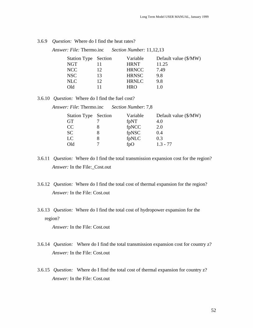
Long Term Model USER MANUAL, January 1999
52
3.6.9 Question: Where do I find the heat rates?
Answer: File: Thermo.inc Section Number: 11,12,13
Station Type Section Variable Default value ($/MW)NGT 11 HRNT 11.25NCC 12 HRNCC 7.49NSC 13 HRNSC 9.8NLC 12 HRNLC 9.8Old 11 HRO 1.0
3.6.10 Question: Where do I find the fuel cost?
Answer: File: Thermo.inc Section Number: 7,8
Station Type Section Variable Default value ($/MW)GT 7 fpNT 4.0CC 8 fpNCC 2.0SC 8 fpNSC 0.4LC 8 fpNLC 0.3Old 7 fpO 1.3 - 77
3.6.11 Question: Where do I find the total transmission expansion cost for the region?
Answer: In the File:_Cost.out
3.6.12 Question: Where do I find the total cost of thermal expansion for the region?
Answer: In the File: Cost.out
3.6.13 Question: Where do I find the total cost of hydropower expansion for the
region?
Answer: In the File: Cost.out
3.6.14 Question: Where do I find the total transmission expansion cost for country z?
Answer: In the File: Cost.out
3.6.15 Question: Where do I find the total cost of thermal expansion for country z?
Answer: In the File: Cost.out

Long Term Model USER MANUAL, January 1999
53
3.6.16 Question: Where do I find the total cost of hydropower expansion for
country z?
Answer: In the File:Cost.out
3.6.17 Question: Where do I find the total cost of the operations and maintenance for
the region?
Answer: In the File: Cost.out
3.6.18 Question: Where do I find the total cost of the operations and maintenance for
country z?
Answer: In the File: Cost.out
3.6.19 Question: Where do I change the cost of the operations and maintenance for a
thermal plant?
Answer: File: Thermop.inc Section Number: 17,18,19
Station Type Section Variable Default value ($/MWh)NGT 17 OMT 8.6NCC 18 OMCC 4.2NSC 18 OMSC 6.7NLC 19 OMLC 8.9Old 19 OMO 8.9
3.6.20 Question: Where do I change the fixed capital cost of new thermal sites?
Answer: File: Thermo.inc Section Number: 1,2
Station Type Section Variable Default valueCC 1 FGCC $109 millionLC 2 FGLC $581 million
3.6.21 Question: Where do I change the fixed capital cost of new hydropower plants?
Answer: File: Hydro.inc Section Number: 1
Change the values of the variable HNinit.

Long Term Model USER MANUAL, January 1999
54
3.6.22 Question: Where do I change the fixed capital cost of new transmission lines?
Answer: File: Lines.inc Section Number: 4
Change the values of the variable PFNFc.
3.6.23 Question: Where do I change the capital cost of extensions to thermal sites?
Answer: File: Thermop.inc Section Number 3
Station Type Section Variable Default value ($/MW)NGT 3 NTexpcost 300000NCC 3 NCCexpcost 412000NSC 4 NSCexpcost 1433333NLC 4 NLCexpcost 857000Old 2 Oexpcost 1000000
3.6.24 Question: Where do I change the capital cost of extensions to existing
hydropower sites?
Answer: File: Hydro.inc Section Number: 5Change values to the variable HOVcost.
3.6.25 Question: Where do I change the capital cost of extensions to existing
transmission lines?
Answer: File: Lines.inc Section Number: 1
Change the values of the variable PFOVc.
3.6.26 Question: Where do I change the values of the CRF for old and new thermal
plants?
Answer: File: Thermo.inc Section Number: 16,17
Change values of the variables crfi, crfni.
3.6.27 Question: Where do I change the values of the CRF for old and new hydro
plants?
Answer: File: Hydro.inc Section Number: 6,7
Change values of the variables crfih, crfnh.

Long Term Model USER MANUAL, January 1999
55
3.6.28 Question: Where do I change the values of the CRF for new transmission lines?
Answer: File: Lines.inc Section Number: 2
Change values of the variable crf.
3.6.29 Question: Where can I change the escalation of fuel costs?
Answer: Thermo.inc Section Number: 9,10
Station Type Section Variable Default valueNGT 9 fpescNT 1.01NCC 10 fpescNCC 1.01NSC 10 fpescNSC 1.01NLC 10 fpescNLC 1.01Old 9 fpescoO 1.01
3.6.30 Question: Where can I change the interest?
Answer:File: Data.inc Section Number: 1
Change the scalar int. The default value is 0.1
3.7 Output Files
3.7.1 Question: Where do I find the total cost (NPV) of the free trade optimization?
Answer: Running the free trade option the total cost is at the top of every output
file.
3.7.2 Question: Where do I find the cost (NPV) to each country from the free trade
optimization?
Answer: In the file: Cost.out
3.7.3 Question: Where do I find the total cost (NPV) of the fixed trade optimization?
Answer: Running the fixed trade option the total cost is at the top of every output
file.
3.7.4 Question: Where do I find the cost (NPV) to each country from the no trade
optimization?
Answer:File: Exp_cost.out Section Number

Long Term Model USER MANUAL, January 1999
56
3.7.5 Question: Where do I see the list of chosen projects from the optimization?
Answer: The output files show the expansions for each country, the type of
technology, and the MW quantities. A list of specific project names is to be coded in a
new output file, yet to be finalized (January 1999).
3.7.6 Question: Where do I find the benefits of joint planning for my country?
Answer: First run the free trade option, taking the final cost, and then run the
fixed trade option taking the final cost. The difference between the two final costs gives
the benefits from joint planning.
3.7.7 Question: Where do I find the benefits of joint planning for SAPP?
Answer: First run the free trade option, taking the final cost, and then run the
fixed trade option taking the final cost. The difference between the two final costs gives
the benefits from joint planning.
3.7.8 Question: Where can I find the annual energy exports over time and the grand
total for my country?
Answer: File: Trade.out Section Number
3.7.9 Question: Where can I find the annual energy imports over time and the grand
total for my country?
Answer:In the File: Trade.out
3.8 Questions Related to The Formulation
3.8.1 Question: What are the pros/cons of choosing expansion to be continuous, rather
than multiples of fixed plant sizes?
Answer: pro- quicker solution time con- round off error
3.8.2 Question: Can I select which variables are continuous, which are fixed multiples,
or must I declare all to be one or the other?
Answer: You can select any or all to be either continuous or discreet

Long Term Model USER MANUAL, January 1999
57
3.8.3 Question: What criteria should I use to decide if a capacity expansion variable
should be continuous, or multiples of a fixed size?
Answer: Two factors: (a) the availability of units in many sizes (simple turbines)
(b) the importance that the unit plays in the solution.
3.8.4 Question: Can I simply round off a continuous capacity variable to the size of the
nearest available unit?
Answer: Yes, that is the suggested solution. If more accuracy is desired, run the
model twice, once with the variable fixed at the rounded up value, once with the rounded
down value.
3.8.5 Question: How are scale economics reflected in the model?
Answer: By associating a large fixed cost with the construction of the initial units
of capacity e.g. initial fuel handling/water treatment/site preparation/transportation/sub-
station costs for thermal, the dam for hydro, right of way purchase and tower construction
for transmission.
3.8.6 Question: Does the model compete units with scale economics against units with
constant returns to scale?
Answer: Yes, simple gas turbines and small coal plants are assumed to have
constant returns to scale; they compete directly with combined cycle gas turbines and
large coal plants; which ever is chosen is dependent on the yearly growth expected in a
region - the larger the MW growth increment, the more likely the model will choose the
units with scale economics, and lower costs. (Another advantage of SAPP wide capacity
planning - fewer, bigger, cheaper (/KWh) units that are least cost if each country uses
only it's own units to satisfy its own demand growth.
3.8.7 Question: Can I substitute my own thermal plants in place of those based on U.S.
experience now in the model?
Answer: Yes, if the performance and cost of technology can be satisfactorily
captured by the parameters used in the model to characterize U.S. technology initial

Long Term Model USER MANUAL, January 1999
58
capital cost, subsequent expansion cost, heat rate, capacity, forced/unforced outage rate,
O&M cost, equipment lifetime, maximum size of expansion.
3.8.8 Question: Why are no capital costs for existing plant in the model?
Answer: These are considered sunk costs; the model considers only costs which
can be avoided.
3.8.9 Question: Which types of costs - incremental, or average - should be used to
populate the model?
Answer: Only incremental costs should be used.
3.8.10 Question : Is the model a discounted cash flow model?
Answer: Yes, with one exception. Equipment purchases where all the money is
paid at the time of the purchase are treated as if the money is paid to the sources of
capital in equal installments. The cash flows of plant and equipment financed over time
by use of a capital recovery factor are correctly captured in the model.
3.8.11 Question: Can I alter the model to handle cases where all the money must be paid
"up front"?
Answer: Yes, but this will require calculating a salvage value at the end of the
planning horizon for the plants equipment, in order to allow the model to add
capacity towards the end of the horizon.
3.8.12 Question: How does the model handle the cost of construction work in progress
("CWIP")?
Answer: It assumes that all dollars are spent in the year in which the plant comes
on line. Thus, any carrying charges for work in progress should be added to the initial
costs of the plant. Alternatively, the model could be modified to allow capital costs to
begin to enter the objective function prior to initial operation, if the spending profile were
specified. Some changes in the service code would be necessary, but none very
complicated or time consuming.

Long Term Model USER MANUAL, January 1999
59
3.8.13 Question: Must the capital cost of a new site include the cost of hook-up to the
grid?
Answer: Yes, the assumption is that when the capital cost is incurred, all infrastructure is
in place to allow the electricity to start satisfying demand.
3.8.14 Question: Are environmental consideration taken into account in the model:
Answer: Not at the present time. The source code could be easily modified to
allow the model to keep track of the environmental impact (SOXNOX/particulate, etc.) of
any SAPP plan, if data were made available by SAPP, or alternatively, typical U.S. plant
data could be used.
3.8.15 Question: Do the capital costs of the default coal plants in the model take into
account the environmental characteristics of the coal burned?
Answer: In an average way - capital costs include the cost of standard scrubbing
equipment found on new coal fired plants installed in the U.S. which met U.S. current
environmental standards for SOX/NOX/Particulate.
3.8.16 Question: How are the smaller thermal units now in place handled by the model?
Answer: The model ignores all units less than - MW, since they likely will never
be used as a substitute for impacts, the key decision considered in the model.
3.8.17 Question: How can thermal units already committed to, but no on line, be entered
into the model?
Answer: By treating their capacity as existing capacity in 2002 if the units are not
expected to be in service by then. They can be treated as new equipment with the
decision variable set at "build" in the period when the unit is expected to enter
service.

Long Term Model USER MANUAL, January 1999
60
3.8.18 Question: Why does the model not include commitment costs alone with dispatch
costs?
Answer: Unit commitment includes the use of many conditional constraints of the
if,then. form. These require many additional integer variables, and would drastically
increase the running time with a less then commensurate increase in realism or accuracy.
3.8.19 Question: Can a more realistic assumption be made regarding the rate of decay
than the constraint percentage assumption used in the model?
Answer: Yes, another formulation which allows arbitrary varying rates of decay
over time is available, but not programmed into the model at the present.
3.8.20 Question: Who is responsible for financing an international transmission
expansion?
Answer: Not specified in the model. Could split the cost into two countries
for some cases.
3.8.21 Question: Should I have different assumptions for the CRFs for a large hydro
project, such as the one in DRC? For example, if the project is developed by a consortium
of RSA, DRC, and some IPPs from out side world, should the CRF in this case is the
same as the one developed solely by DRC?
Answer: Not specified. Could be done by calculating different CRFs according to
different assumptions.
3.8.22 Question: If the model is not run on a yearly basis (i.e., expansion for every
year), what is the assumption for the capacities in the years not in the model? Are you
assuming a constant capacity in the years?
Answer: Not clear at the time being.
3.8.23 Question: If the capacities in the years not modeled are not constant, then what
are the capacities?
Answer: No answer yet.

Long Term Model USER MANUAL, January 1999
61
3.8.24 Question: What are the capital costs associated with the variations mentioned in
22 and 23?
Answer: No answer yet.
3.8.25 Question: What are the production costs associated with the variations mentioned
above?
Answer: Not simulated. A very rough estmation.
3.8.26 Question: Is it possible to improve your computation time to a one day limit with
a convergence criterion of 0.1 %?
Answer: Model can make optimal runs (0.0%) within several hours and with
0.3% in less than half an hour.
3.8.27 Question: Is it possible to reduce the memory requirement?
Answer: Different algorithm will do but need more time and money to have it
done.
Preferable a third year study.
3.8.28 Question: Is it possible to have a window based, user friendly interface such that
we do not have to mess-up with the program?
Answer: Possible. But not this year.
3.8.29 Question: Is it possible to have window based interface to change data?
Answer: Possible if there is a third year study.
3.8.30 Question: It is desirable to have an algorithm to select the 6 day types, such that
the total yearly energy is about right while retaining the peaks, especially for ESKOM.
Answer: Possible and we need to do this.


Long Term Model USER MANUAL, January 1999
CHAPTER 4
THE FULL LONG-RUN MODEL
This chapter has four sections, each with its own appendix.
Section 1: The load balance, or supply/demand equations, which ensures that user
specified demands are met for each of the hours in the six representative day types in the
model-summer/winter peak, off-peak, and average days. (See Appendix 1A and 1B)
Section 2: The capacity constraints, which insure that each plant’s generation
does not exceed the properly derated installed capacity for the day types in the model.
(See Appendix 2)
Section 3: The reliability constraints, which insure that a proper reserve margin is
maintained between installed capacity and peak period demand in every period. (See
Appendix 3)
Section 4: The objective function, which calculates the present value of all
operating costs and all capital costs for new equipment over the planning horizon. (See
Appendix 4)
4.1 The Demand/Supply Equations
4.1.1 The Demand for Electricity
The model is driven by the “typical hour/day/season/year” chronological demand
approach taken by many of the latest commercial models, rather than the load duration
curve methodology used in earlier approaches. The appendix to this chapter gives all the
input files necessary to create the demand drivers for the model. Demands and supplies
are for the utilities in SAPP, rather than for the SAPP countries. Thus, municipalities or
others in the SAPP countries which generate and use their own electricity are not
considered in calculating either the forecast demand, or the power available to meet such
demands.

Long Term Model USER MANUAL, January 1999
64
The model is set up to model demand in five representative periods in the future,
starting in year 2000 to allow completion of all SAPP projects now underway.
The model allows the user to decide how many years each period will represent -
every year (2000, 2001, 2002, 2003, 2004) or every other year (2000, 2002, 2004, 2006,
2008) every third year, etc., etc., by selecting the value for scalar “n” in the model. (See
the appendix to this section.) The model automatically adjusts the yearly growth rates
and the cost function to insure the model fully adjusts to the selection made by the user,
allowing a range of planning horizons - 5, 10, 15, or 20 years
In all cases, no capacity expansion is allowed in the initial (2000) year; those
construction projects SAPP indicated would be completed by that date are included as
installed capacity. Thus, the first year’s optimization involves only dispatch of existing
capacity against the first year’s demand.

Long Term Model USER MANUAL, January 1999
65
TABLE 4.1: SADC & SOUTHERN AFRICA POWER POOL - GDP & CAPACITY GROWTH RATES - 1996-2020
1996-2020 MaximumDemand
1996MW
GDP Growth(annual average rates)
Electricityto GDP
Elasticity(underlying)
ElectricityIntensiveProjects
MW
DemandSide M'mentby 2020 (H)
MW
Maximum Demand(internal - 2020)
Maximum Demandgrowth rates 1996-2020
Comments
LOW% p.a.
MEDIUM% p.a.
HIGH% p.a.
LOWMW
MEDIUMMW
HIGHMW
LOW% p.a.
MEDIUM% p.a.
HIGH% p.a.
Angola 181 1.5% 3.0% 6.0% 1.26 1000 38 765 1111 2004 6.2% 7.9% 10.5% Mining & mineral beneficiation
Botswana 222 3.6% 4.2% 5.9% 1.01 60 47 529 606 903 3.7% 4.3% 6.0% Industry plants
Lesotho 76 3.5% 6.0% 8.0% 1.04 16 171 312 501 3.4% 6.1% 8.2%
Malawi 164 2.0% 3.0% 5.5% 1.16 34 268 346 693 2.1% 3.2% 6.2%
Mozambique 192 3.0% 5.0% 7.0% 1.36 2000 40 1481 2299 3662 8.9% 10.9% 13.1% MOZAL, I&S (Maputo),Moatize Coal, other minerals
Namibia 321 3.5% 5.0% 6.0% 1.02 1000 67 1210 1704 2265 5.7% 7.2% 8.5% Mining developments
South Africa 26382 2.0% 3.8% 5.5% 1.05 1500 7900 40244 62199 95108 1.8% 3.6% 5.5% Mining & mineral beneficiation
Swaziland 140 2.6% 3.6% 4.6% 1.04 29 251 315 400 2.5% 3.4% 4.5%
Tanzania 412 2.4% 4.0% 5.3% 1.30 500 86 1068 1672 2452 4.0% 6.0% 7.7% Mining developments
Zambia 1028 2.4% 4.0% 5.8% 1.09 250 215 1928 2866 4511 2.7% 4.4% 6.4% Mining back to capacity
Zimbabwe 1744 2.8% 4.0% 5.7% 1.04 400 366 3490 4626 6982 2.9% 4.1% 5.9% Mining & mineral beneficiation
SADCtot/weighted av
30862 2.1% 3.8% 5.6% 1.06 6710 8839 51406 78055 119483 2.0% 3.8% 5.7%
South Africa 26382 2.0% 3.8% 5.5% 1.05 1500 7900 40244 62199 95108 1.8% 3.6% 5.5%
Rest of SADC 4480 2.7% 4.1% 5.8% 1.10 5210 939 11162 15856 24374 3.6% 5.0% 6.9%
Scenarioprobabilities
0.40 0.45 0.15
Compiled by: Peter B. Robinson, July 1998

Long Term Model USER MANUAL, January 1999
66
Yearly demand growth rates which differ by scenario (hi, medium, low, growth), by time
period, and by country (parameter “dgrowth1(z)”, to “dgrowth5(z)” in the appendix to this
section) can be specified by the user. Table 4.1 (page 2) gives country growth rates for the
planning horizon as estimated by Dr. Peter Robinson for the July 1998 Cape Town workshop.
The medium growth rates in the next to last column are the default values now entered in the
growth rate tables, but can be over-ridden by the user. The program automatically converts the
yearly growth rates into the proper growth rates for the periods of varying length in the model, as
indicated in the section “parameter (dgr(z,ty)” in the appendix.
Within each year – two seasons – summer and winter – are modeled. The summer period
contains nine months (273 days), while the winter contains three months (91 days). Within each
season, three days – a peak day, an off-peak day, and an average day – are modeled.
Within the summer season, there are 39 peak days, 39 off-peak days, and 195 average
days. Within the winter season, there are 13 peak, 13 off-peak, and 65 average days.
The 24 hour individual country consumption patterns during the base year 2002 for each
of the two seasons - summer and winter - and each of the three day types - peak, off-peak, and
average - are entered by users in the tables “Base(ts,td,z)” titled: “base winter peak”, “base
winter off-peak”, “base winter average”, “base summer peak”, “base summer off-peak”, “base
summer average”.
These tables are found in the appendix, with default values obtained by;
• projecting the July 24, 1997 (winter peak) data for all countries used in the short term
model to the base year 2000 by use of the current growth rates of electricity demand
for each SAPP country provided by SAPP;
• creating the other five day types from projected winter peak consumption by use of
day factors - off-peak = 0.7, peak = 1.0, average = 0.8 - and season factors - summer
= 0.9 and winter = 1.0.
Users of the model can choose any of three options for modeling the hourly demand each
day:
Option #1: (The Default Option) A weighted 6-hour version of the 24-hour data,
containing one off-peak hour (hr9), three peak hours (hr19, hr20, hr21),
and two average hours – one an average of eight such night hours, “avnt,”
and one an average of 12 average day hours, “avdy.” The two average

Long Term Model USER MANUAL, January 1999
67
hours are calculated to insure that total energy use is the same for the six-
hour version as the 24-hour version.
Option #2: 24-hour demand data for each country.
Option #3: A one-hour peak demand version (hr19 only) used for debugging purposes
only.
In all cases, the base day type tables in the appendix are called; the choice of the one-
hour, six-hour, or 24-hour version is dictated by the use of the “$ontext” and “$offtext” GAMS
commands.
All this comes together in creating the demand driver for the model, parameter
“Dyr(ty,ts,td,th,z)”, which is country “z”’s MW demand in year “ty” (“ty” = 2002, and then 2, 3,
or 4 year periods as chosen by the user) in season “ts” (“ts” = winter, summer) in day “td” (“td”
= peak, off-peak, average) in hour “th” (“th” = hr19 for the one-hour model; hr9, avnt, hr19,
hr20, hr21, and avdy in the 6-hour model; hr1 to hr24 in the 24-hour model): Combining the
yearly growth assumptions with the base year day type demand data, we have;
Dyr(ty,ts,td,th,z) = Base(ts,td,th,z)dgr(ty,z)
In GAMS notation (Main.gms file, section 2)
Parameter Dyr(ty,ts,td,th,z); Dyr(ty,ts,td,th,z)=july2400(ts,td,th,z) * dgr(z,ty)
Next, the impact on these demands of domestic distribution loss and demand-side
management must be considered.
Table “DLC(z)” in the appendix – the domestic loss coefficient in the model – is applied
to the demand value to allow for electricity loss within each SAPP region; it converts demand at
the customer meter into demand at the generating station. Thus, it is important that demand
measured at the customer meter be entered in the tables, not demand at the generation station.
The demand-side management (“DSM”) parameter – (“LM(th,z)” in the appendix to this
chapter) – allows SAPP member specified “DSM” options to fractionally adjust up or down the
load shapes of the representative days in the model, with user-specified costs of such programs
entered into the objective function. It should be emphasized that the model in its current form

Long Term Model USER MANUAL, January 1999
68
does not compete “DSM” against normal supply side options to obtain the least cost mix of
“DSM” and capacity expansion. It simply allows various “DSM” options with known costs and
benefits to be entered into the model to see “off-line” if they are cost effective when compared to
supply alternatives. It is planned to add “DSM” to the optimization formulation at a later date, as
described in Appendix 2 to this section.

Long Term Model USER MANUAL, January 1999
69
Table 4.2a Optional New SAPP Generating Capacity(A Revision of Year 2 Interim Report Appendix V, - January 29, 1999)
Country Powerstation # ofUnits
Unit Size(MW)
TotalAddedMW)
Cost $million
TypeT/H/PS
Cost$/kW
HRBtu/KWh
Fuel$/MWh
O & MCost$/MWh
Optional ProjectsAngola Cambambe (Ext.) 2 45 90 HAngola Capanda II 2 130 260 300 H 1153
Botswana Moropule (Ext.) 2 120 240 420 T 1750
DRC Inga 3 3500 4900 1400**DRC Grand Inga ST1 4750 9780 H 2059DRC Grand Inga ST2 4750 6330 H 1332DRC Grand Inga ST3 4750 6120 H 1288DRC Grand Inga ST4 4750 6070 H 1278
Lesotho Muela 3 24 72 58 H 805
Malawi Kaphichira Phase1 * 2 32 64 HMalawi Kaphichira Phase 2 2 32 64 24 H 375Malawi Lower Fufu 2 45 90 119 H 1322Malawi Mpatamanga 5(?) 63(?) 315 335 H 1063Malawi Kholombidzo 2 35 70 330 H 4714
Mozambique Mepanda Uncua 5 400 2000 2800 H 1400***Mozambique Cah. Bassa N. (Ext.) 1240 1054 H 850
Namibia Kudu (Gas) 1 750 750 650 T 866Namibia Epupa 1(?) 360 360 408 H 1133
South Africa Komati A (Recomm). 5 5x90 450 125 T 277 12876 5.154 5.416South Africa Grootvlei (Recomm). 6 5x190+1x
1801130 123 T 109 12186 7.673 4.236
South Africa Komati B (Recomm). 4 4x110 440 238 T 542 12876 6.026 0.68South Africa Camden (Recomm). 8 190 1520 164 T 108 12186 5.855 4.122South Africa PB Reactor 10 100 1000 844 T 844 7583 3.4 0.2South Africa Lekwe 6 659 3950 4056 T 1027 9890 4.119 0.6South Africa Pumped Storage A 3 333 999 373 PS 374South Africa Pumped Storage B 3 333 999 377 PS 378South Africa Pumped Storage C 3 333 999 379 PS 380South Africa High head UGPS 2 500 1000 237 PS 237South Africa Gas Turbine 4 250 1000 324 T 324 9478 58.66 0.646
Tanzania Ubungo (Gas) 1 40 40 24 T 600 9045 25.6 3.405Tanzania Tegeta (Gas) 10 10 100 90 T 900 11055 140.0Tanzania Kihansi 3 60 180 270 H 1500Tanzania Rumakali 3 74 222 439 H 1977Tanzania Ruhudji 4 89.5 358 515 H 1438
Zambia Itezhi-Tezhi 2 40 80 74 H 927Zambia Kafue Lower 4 150 600 450 H 750Zambia Batoka North 4 200 800 898 H 1122Zambia Kariba North (Ext.) 2 150 300 223 H 743
Zimbabwe Hwange Upgrade 1 84 84 130 T 1547Zimbabwe Hwange 7 & 8 2 300 600 554 T 923 9574 3.427Zimbabwe Gokwe North 4 300 1200 960 T 800 9248 3.023Zimbabwe Batoka South 4 200 800 898 H 1122Zimbabwe Kariba South (Ext.) 2 150 300 200 H 667
Commited ProjectsSouth Africa Majuba* 6 3x612,
3x6673837 T 10340 5.734 0.495
South Africa Arnot 3-6 Recomm.* 4 4x330 1320 T 10185 3.223 0.718 *Commissioned by 2000, ** Estimated, ***Estimated and assumed given 664 did not include dam

Long Term Model USER MANUAL, January 1999
70
Table 4.2b SAPP Thermal Generation Data for Existing Plants
Country &Station Name
PGmax(MW)
Country &Station Name PGmax
(MW)Angola 113Botswana 118 RSA
Arnot 1320Mozambique Duvha 3450 Beira 12 Hendrina 1900 Maputo 62 Kendal 3840 Namibia Kriel 2700 Vaneck 108 Lethabo 3558 Paratus 24 Majuba 1836Zimbabwe Matimba 3690 Hwange 956 Matla 3450 Munyati 80 Tutuka 3510 Harare 70 Koeberg * 1840 Bulawayo 120Swaziland 9 (* Nuclear)
Table 4.2c SAPP Hydropower Generation Data for Existing Plants
Country &Station Name
Hmax(MW)
Country &Station Name
Hmax(MW)
Angola 121 Malawi56 Knula 21437 Tedzani 6437 Tedzani 6437
DRC RSA Inga 1775 Gariep 320 Nseki 248 Vanderkloof 220 Nzilo 108 Palmiet # 400 Mwadingusha 68 Drakensbur# 1000 Koni 42Mozambique Zimbabwe HCB 2075 KaribaSouth 666 Chic-Cor-Mav 81 ZambiaNamibia KaribaNorth 600 Ruacana 240 Kafue 900Swaziland 40 Victoria 100
(# Pumped)

Long Term Model USER MANUAL, January 1999
71
Finally, combining the yearly growth assumptions with the “DLC” and “DSM” data
allows the specification of the right-hand side of the load balance equation, which specifies: for
each hour in each day in each season in each year, the demand at the generating station that must
be met inclusive of the effect of distribution line loss and “DSM” programs is then;
4.1.2 The Supply Side
The demand in a given region can be met from a variety of energy sources: (a) existing
thermal sites, (b) new thermal sites, (c) existing hydro sites, (d) new hydro sites, (e) net imports
(imports less exports), (f) paying an unserved energy cost, (g) pumped storage.
Within each region, generating sites are identified which contain generating plants. For
purposes of dispatch, all plants at a site are collectively dispatched. Generation variables, in
MW, for the sites are:
PG(ty,ts,td,th,z,i) = generation from existing thermal site “i”
PGNT(ty,ts,td,th,z,ni) = generation from new gas turbines at site “ni”
PGNSC(ty,ts,td,th,z,ni) = generation from new small coal plants at site “ni”
PGNCC(ty,ts,td,th,z,ni) = generation from new combined cycle plants at site “ni”
PGNLC(ty,ts,td,th,z,ni) = generation from new large coal plants at site “ni”
H(ty,ts,td,th,z,ih) = generation from existing hydro site “ih”
Hnew(ty,ts,td,th,z,nh) = generation from new hydro site “nh”
PGPSO(ty,ts,td,th,z) - PUPSO(ty,ts,td,th,z) = net generation from old pumped hydro
sites (“PGPSO” is generation supply, “PUPSO” is pump demand)
PGPSN(ty,ts,td,th,z,phn) - PUPSN(ty,ts,td,th,z,phn) = net generation from new pumped
hydro sites (“PGPSN” is generation supply, “PUPSN” is pump demand)
Default value characteristics of new and old plants are based on data furnished by SAPP
members, as well as data representative of the latest U.S. plants, as described below.
[ ][ ])z(DLC)z,th(DSM)z,th,td,ts,ty(Dyr −

Long Term Model USER MANUAL, January 1999
72
(a) Existing Thermal Sites
Tables 4.2a, b, c plus Table “PGOinit(z,i)”, in the appendix to section 2 (The Capacity
Constraint Module), lists the current MW capacities of the existing thermal sites in the model
(including Nuclear, Koeberg, SSA) -- in addition to the set developed for the short-run model,
(see the first year report for details), committed projects listed in Table 4.2 are also included.
NSA has 12 sites (10 existing, 2 committed), Zimbabwe 4 sites, Namibia and Mozambique 2,
and Angola, Botswana, Lesotho, Malawi, Swaziland, Tanzania, and Zambia have single sites, all
coal fired. In addition, South Africa has one nuclear plant. The rows in Table “PGOinit(z,i)” are
the locations listed in order of the “z” index assigned - e.g., Ang (Angola) is z=1, Bot
(Botswana) is z=2, etc., Zimbabwe is z=14. (Note Mozambique and RSA are divided into two
regions -north and south -to recognize the reality of the split supply situation in Mozambique,
and the split demand situation in RSA). The site index “i” follows the column index “stat i”.
Power generation in year “ty”, season “ts”, day type “td”, hour “th”, at old site “i” in
country “z” is given by the continuous non-negative variable “PG(ty,ts,td,th,z,i)”. Thus
“PG(1,1,1,1,1,1)” is the MW contribution of Angola (“z”=1) site 1 (stat 1) during year 1 (2002)
in season 1 (winter) in day type 1 (off-peak) during hour 1 (hour 1 for the 24 hour model, hour 9
for the 6 hour version).
(b) New Thermal Sites
Table 4.2 lists the characteristics of new or recommissioned thermal plants under
consideration by SAPP. South Africa is considering 7 new thermal plants, including one new
nuclear plant, Zimbabwe 3, Tanzania 2, and Botswana, Mozambique, and Namibia one each. In
addition to utilizing the capacity of the existing coal fired sites described above and these new
plants, the model allows development and construction of four types of new fossil fuel sites in
selected countries where the fuel is available. A complete description of the four options will be
given in the capacity expansion section later in the report, dealing with the values of
“PGNinit(z,ni)”.
• a small variable capacity simple cycle gas combustion turbine, available in all
countries. Power generation in MW from such sites is given by the continuous
variable “PGNT(ty,ts,td,th,z,ni)” in the model

Long Term Model USER MANUAL, January 1999
73
• a small fixed capacity sub-critical coal plant, in RSA, Botswana, Zimbabwe, and
Tanzania. Power generation levels are given by “PGSC(ty,ts,td,th,z,ni)”.
• a variable capacity combined cycle combustion turbine in those countries where
natural gas could be available - Namibia, RSA, Mozambique, Tanzania, and Angola.
Power generation from such sites is given by “PGNCC(ty,ts,td,th,z,ni)”
• a large variable capacity pulverized coal site, available only in RSA Power generation
levels are given by “PGNLC(ty,ts,td,th,z,ni)”
The nominal values of these four plants’ technical and economic data in the model are
taken from a recent survey of typical plants constructed world-wide. Users can override the
nominal data, and enter the specifics of fossil fuel projects into the tables described in the
capacity expansion section later in the report.
(c) Existing Hydro Sites
Table 4.2, plus Table “HOinit(z,ih)” - “z” the row (country) index, “ih” the column (site)
index - in the appendix to section 2 (The Capacity Constraint Module), lists the current MW
capacities of the existing hydro sites in the model. Angola, Tanzania, and DRC have 5 sites
each, SWZ, and ZAM 3 each, MWI, NMZ, NSA, and SSA have 2 sites, and the rest of the
countries in the table have one each. A complete description of the sites will be given later in the
report.
MW output from the existing sites is given by the variable “H(ty,ts,td,th,z,ih)”.
(d) New Hydro Sites
Table 4.2, plus Table “HNinit(z,nh)” - again “z” the row (country) index, “nh” the
column (new site) index - in the appendix to section 2 lists the hydro sites under consideration by
SAPP members. MWI has 4 sites, TAZ and ZAM 3, ZIM 2, and ANG, LES, NMZ, NAM, and
DRC one each. The options, as expected, are dominated by the expansions of DRC’s Grand Inga
hydro site, which accounts for over two-thirds of planned hydro capacity. Total expansion plans
involve the possible construction of almost 22,000 MW of new capacity, based on the 1995
SAPP official list of capacity expansion projects, contained in Table 4.2.
MW output from the new sites is given by the variable “Hnew(ty,ts,td,th,z,nh)”.

Long Term Model USER MANUAL, January 1999
74
(e) Net Imports
Figures 2.1 and 2.2 in Chapter two, and Tables “PFOinit(z,zp)” and “PFNinit(z,zp)” the
appendix to section 2 list the initial MW capacities of the existing and proposed lines
respectively linking the 14 regions which make up SAPP in the model. The matrices are
symmetric, so that power flow capacity from country A to B is the same as B to A, with the
exception of DC lines.
Transmission losses on the lines are given in tables “PFOloss(z,zp)” for existing lines,
and “PFNloss(z,zp)” for new lines in the appendix to this section.
MW power flows from region “z” to “zp” on old lines are given by the variables
“PF(ty,ts,td,th,z,zp)” while flows on the new lines are given by the variables
“PFnew(ty,ts,td,th,z,zp)”. Using this notation, and accounting for line losses reducing the
amount of power arriving at region “z”, net imports for region “z” in a given hour would be;
PF(ty, ts, td, th,zp, z)(1 − PFOloss(zp,z))
imports arriving on old lines6 7 4 4 4 4 4 4 4 4 8 4 4 4 4 4 4 4 4 − PF(ty, ts, td, th, z,zp)
exports sent on old lines6 7 4 4 4 8 4 4 4
zp
∑
+ PFnew(ty, ts, td, th,zp,z)(1 − PFNloss(zp, z))
imports arriving on new lines6 7 4 4 4 4 4 4 4 4 4 8 4 4 4 4 4 4 4 4 4 − PFnew(ty, ts, td, th,z, zp)
exports sent on new lines6 7 4 4 4 4 8 4 4 4 4
zp
∑
(f) Unserved Energy
Each region can choose not to meet demand by allowing unserved energy to enter the
supply side of the demand/supply balance equation. The variable “UE(ty,ts,td,th,z)” gives the
MW value of the amount. The scalar “UEcost” in the appendix to section 4 sets the cost/MWh
of unserved energy. The nominal value is $5000, but it can be set at whatever value users want
to adopt.
(g) Pumped Storage
At least two SAPP members (RSA and Tanzania) either have, or are planning to add,
pumped storage as a means of peak-shaving/valley filling their 24 hour demand profiles. Table
4.2 contains data on the four known pumped storage projects planned by RSA. Pump storage

Long Term Model USER MANUAL, January 1999
75
uses electricity off-peak to pump water up to reservoirs, which are then discharged during peak
periods.
The hourly (MW) amount of on-peak generating at the two existing pump storage sites in
RSA will be indicated by the non-negative variable “PGPSO(ty,ts,td,th,z)”, while the hourly
MW amount of off-peak pumping will be indicated by the non-negative variable
“PUPSO(ty,ts,td,th,z)”. The power available for generation is less than the power used to pump
because of pump storage system loss, given by the parameter “PSOloss”. Pumped storage
facilities are assumed to operate on a 24 hour cycle - e.g. what is pumped up in a night must
come down in the same day. Thus, the sum over all hours in a day of “PGPSO(⋅)” cannot exceed
the sum overall hours of “PUPSO”, less loss;
PGPSO(ty, ts, td, th,z) ≤ PUPSO(ty, ts, td, th, z)(1 − PSOloss)th∑
th∑
In GAMS format, equation “oldpumped” is; (Main.gms file, section 25)
Equation Oldpumped;Oldpumped(ty,ts,td,z) $PGPSOinit(z) ..sum(th, Mtod(th) * PGPSO(ty,ts,td,th,z)) =L=sum(th, Mtod(th) * PUPSO(ty,ts,td,th,z))*(1-PSOloss);
The GAMS equation indicates this is always an equality at an optimum solution, since it
was decided not to include the possibility of longer term storage in the model.
The default value of “PSOloss” is set at 0.3 in the model.
The model enters pumped storage into the load balance equation on the supply side;
hence “PGPSO(⋅)” enters with a positive sign, while “PUPSO(⋅)” enters with a negative sign; e.g.
Generation plus net imports +PGPSO(⋅) - PUPSO(⋅) = Demand
Pumped storage from new sites (indexed “phn”) enters into the model in a similar fashion, except
the variables are “PGPSN(⋅)” and “PUPSN(⋅)”.

Long Term Model USER MANUAL, January 1999
76
In GAMS format, equation “Newpumped” is; (Main.gms file, section 25)
Equation Newpumped;Newpumped(ty,ts,td,z,phn) $PHNinit(z,phn) ..sum(th, Mtod(th) * PGPSN(ty,ts,td,th,z,phn)) =L=sum(th, Mtod(th) * PUPSN(ty,ts,td,th,z,phn) * (1-PSNloss(phn)));
4.1.3 The Full System Load Balance Equation
The load balance equation - “Equation Demand” in the model - requires that for all time
periods for each country “z”, the sum of MW generation from:
• existing thermal sites - “PG(⋅)”
• new thermal sites - “PGNT(⋅)”, “PGNCC(⋅)”, “PGNSC(⋅)”, “PGNLC(⋅)”
• net imports over existing transmission lines - “PF(⋅,)(1-PFOloss(zp,z)” - “PF(⋅,z,zp)”
• net imports over new transmission lines -
“PFnew(⋅,zp,z)(1-PFNloss(zp,z))” - “PFnew(⋅,z,zp)”
• existing hydro sites - “H(⋅)”
• new hydro sites - “Hnew(⋅)”
• old pumped storage - “PGPSO(⋅) - PUPSO(⋅)”
• new pumped storage - “PGPSN(⋅) - PUPSN(⋅)”
plus unserved energy
• “UE(⋅)”
must be greater than or equal to
• Demand - “Dyr(⋅)”
• less DSM - “LM(⋅)”
• times domestic loss - “DLC(z)”.
all this is entered into the model using GAMS notation as equation “Demand”; (Main.gms file,
section 26)

Long Term Model USER MANUAL, January 1999
77
EQUATION Demand;Demand(ty,ts,td,th,z).. sum(i$(PGOinit(z,i) GT 1), PG(ty,ts,td,th,z,i))+ sum(ni$(fpNT(z,ni) GT 0), PGNT(ty,ts,td,th,z,ni))+ sum(ni$(fpNCC(z,ni) GT 0), PGNCC(ty,ts,td,th,z,ni))+ sum(ni$(fpNSC(z,ni) GT 0), PGNSC(ty,ts,td,th,z,ni))+ sum(ni$(fpNLC(z,ni) GT 0), PGNLC(ty,ts,td,th,z,ni))+ sum(zp$(PFOinit(zp,z) GT 9), PF(ty,ts,td,th,zp,z)*(1-PFOloss(zp,z)) - PF(ty,ts,td,th,z,zp))+ sum(zp$(PFNinit(zp,z) GT 9), PFnew(ty,ts,td,th,zp,z)*(1-PFNloss(zp,z)) - PFnew(ty,ts,td,th,z,zp))+ sum(ih, H(ty,ts,td,th,z,ih))+ sum(nh, Hnew(ty,ts,td,th,z,nh))+ UE(ty,ts,td,th,z)
+ PGPSO(ty,ts,td,th,z) - PUPSO(ty,ts,td,th,z)+ sum(phn$PHNinit(z,phn),PGPSN(ty,ts,td,th,z,phn))- sum(phn$PHNinit(z,phn),PUPSN(ty,ts,td,th,z,phn))
=G= DLC(z) * (Dyr(ty,ts,td,th,z) - LM(z,th));
(Note: the sum is over the only those new units which are actually in existence - e.g. those plants
with positive initial capacity (“PGOinit” > 0) or those with positive fuel prices (“fp” > 0))
4.2 The Capacity Constraint Module
This section will be organized by site type, considering the capacity constraints in
sequence of (a) old thermal sites, (b) old hydro sites, (c) new thermal sites, (d) new hydro sites,
(e) old transmission lines, (f) new transmission lines, and (g) pumped storage.
In all cases, the model will allow no additions to capacity in 2000, the initial year of the
horizon; those the SAPP delegates indicated were under way at the July 1998 workshop will be
treated as capacity already installed. These projected initial capacities as of 2000 are included in
the following tables:
• Thermal: Table “PGOinit(z,i)”, totaling 33,100 MW
• Hydro: Table “HOinit(z,ih)”, totaling 8380 MW
• Transmission: Table “PFOinit(z,zp)”, totaling 14,430 MW
• Pumped Storage: 1400 MW
These capacities are based on installed capacity by plant name, taken from the earlier
short run model, and committed new capacity, by plant name, given in Table 4.2, in section 1.
Thus, only the optimal dispatch problem is solved in 2000, capacities being fixed: this means the

Long Term Model USER MANUAL, January 1999
78
year 2000 can be run in isolation from the rest of the program, since no decision in 2000 affects
subsequent years.
When calculating the available capacity in a time period, the yearly nameplate capacity
must be derated, by the expected forced and unforced outage rates. Since forced outages by their
nature, can occur anytime, peak or off-peak, the yearly nameplate capacity must be derated by
the expected forced outage rate for all operating periods, peak or off-peak. On the other hand,
the timing of unforced, or planned outages for preventive maintenance can be chosen by the
utility. Since generating capacity is more valuable during periods of peak demand than during
off-peak periods, unforced outages are scheduled during off-peak periods. However, unforced
outage rates are given in terms of annual percentage. The off-peak unforced outage rate is
slightly larger than the annual rate, the peak unforced outage rate is zero, and the weighted
average of the two rates equals the annual rate.
The thermal capacity constraints enter the model by day type. Hydro and transmission
capacity will be derated only by forced outage rates, as will be explained below.
In addition, users can specify limits on new construction in the early years to insure
sufficient construction time is available to complete the installations.
Since the model is a long-term year model, the likelihood that existing plants will
deteriorate due to old age, and be unable to generate their initial capacities must be taken into
account.
The model does this by introducing a user specified decay parameter “Decay(i)”, a
function of the technology type, giving the yearly percent reduction in generating capability,
which applies to each site in each country, which is introduced into a generic capacity constraint
in the following way.
A generic capacity constraint requires that generation in year “ty”, “PG(ty,ts,td,th,z,i)”,
respect the available installed capacity in year “ty”, equal to the sum of the initial capacity -
adjusted for decay - plus the capacity added up to and including “ty” - again, adjusted for decay,
properly derated for peak and off-peak periods;
[
] typedayforderate)inaddedcapacityforfactordecay()inaddedcapacity(
)factordecay)(capacityInitial()i,z,th,td,ts,ty(PGty
1∑
=τ
ττ+
≤

Long Term Model USER MANUAL, January 1999
79
Assuming decay takes place at a constant percent per period “ty”, the right hand side of
the expression would be:
For example: if “ty” = 3, the expression would be
4.2.1 Old Thermal Sites
During all times within a given year “ty”, the generation levels given by the variables
“PG(ty,ts,td,th,z,i)” must respect the properly derated site capacity available in that year. Initial
MW capacities for the sites are given in Table “PGOinit(z,i)” in the appendix to this section.
The value of the decision variable “PGOexp(ty,z,i)” determines the amount of new MW capacity
installed at site “i” in year “ty”.
The user can select two options for modeling capacity expansion at existing sites -
treating “PGOexp(ty,z,i)” as a continuous variable, or as an integer variable which allows only
fixed multiples of a given size plant.
Figures 4.1a and 4.1b show the two possible ways of modeling capacity expansion at an
already developed site. Both represent the initial capacity by the parameter “PGOinit(z,i)”, and
both have upper bounds on the total expansion possible at a site “PGOmax(z,i)” (tabled in the
appendix to this section). They differ in the way the expansion is handled.
Figure 4.1a plots available capacity at site “i” as a function of the dollars expended on
new capacity, if it is assumed that additional capacity is available in multiples of fixed plant
sizes, indicated in Figure 4.1a as the step width, “PGOexpstep(z,i)”, tabled in the appendix to
this section.
[] typedayforderate)Decay1()inaddedCapacity(
)Decay1)(CapacityInital(ty
1
ty
ty
∑=τ
τ−−τ+
−
[]derate)Decay1)(3inaddedCapacity()Decay1)(2inaddedCapacity(
)Decay1)(3inaddeCapacity()Decay1)(CapacityInitial(01
23
−+−+
−+−

Long Term Model USER MANUAL, January 1999
80
FIGURE 4.1a: Expansion as fixed multiples of a given size, e.g., “PGOexp(ty,z,i)” = 0,1,2,3
}
}
}PGOexpstep(z,i)
expenditures, Oexpcost(z,i)PGOexpstep(z,i)PGOexp(ty,z,i)
PGOinit(z,i)available capacity in MW, PGOinit(z,i)+PGOexpstep(z,i)*PGOexp(ty,z,i)
PGOmax(z,i)+PGOinit(z,i)
Oexpcost(z,i)*PGOexpstep(z,i)
The cost of a single expansion - the step height - is given by the product of the parameter
“Oexpcost(z,i)” -which gives the cost/MW - times “PGOexpstep(z,i)”, the step width, in MW. If
the integer decision variable “PGOexp(ty,z,i)” is defined as the number of units of size
“PGOexpstep(z,i)” (the step width) installed in year “ty”, then it must be true that capacity
utilization in “ty” at site “i” cannot exceed the initial capacity plus the cumulative expansion up
to and including that made in year “ty” e.g.;
PG(ty, ts, td, th,z,i) ≤
PGOinit(z, i) + PGOexpstep(z,i)PGOexp(tyb,z, i)tyb=1
ty
∑
* derate for day type.
PGOexp(ty,z,i) = 0, 1, 2, 3...
Further, the total expansion over all periods at site “i” cannot exceed the maximum additional
capacity allowed, “PGOmax(z,i)”; - e.g., letting “T” be the last year of the horizon;
PGOexpstep(z, i)PGOexp(tyb, z, i) ≤ PGOmax(z, i)tyb=1
T
∑

Long Term Model USER MANUAL, January 1999
81
FIGURE 4.1b - Expansion as a continuous variable, e.g., “PGOexp(ty,z,i) ≥ 0
expendituresPGOmax(z,i)+PGOinit(z,i)
available MW capacityPGOinit(z,i)
Alternatively, Figure 4.1b assumes expansion to be a continuous, rather than in fixed
multiples of a given plant size. Here it is assumed that there are enough variations in the size of
the units available in the market place to allow the expansion variable to be considered
continuous, and then rounded off by the user to the nearest size available for the technology in
question. If this assumption is made, the utilization equation is identical in form to the preceding
equation, except the variable “PGOexp(tyb,z,i)” is declared positive, rather than integer.
In summary, the capacity constraint for existing thermal units is
)0(positiveor...)3,2,1,0(egerinteither)i,z,tyexp(PGO
typedaybyderate)i,z,tybexp(PGO)i,z(stepexpPGO)i,z(PGOinit)i,z,th,td,ts,ty(PGty
1tyb
≥
+≤ ∑
=
The choice of which to use is up to the user. There is no “free lunch” in modeling; while
assuming capacity expansion is possible only by adding multiple units of a given size is closer to
reality, the user will pay a substantial run time penalty if that route is taken.
Conversely, if the continuous approach is taken, while run times are dramatically
reduced, the error caused by rounding off to the nearest available unit size may cause problems.

Long Term Model USER MANUAL, January 1999
82
Because of construction time lags, no construction is allowed in year 1 - e.g.,
“PGOexp(“yr1”,z,i)” = 0.
The capacity constraint equation needs to reflect the gradual decay in generating
capability as the units age, utilizing the modeling method described previously. Letting
“DecayPGO” be the annual decay rate appropriate for each old thermal site (defalut values tabled
in the appendix) and recalling that periods can have a user specified number of years “n” per
period, (users choose “n” by selecting parameter “DW”), we have the following modification of
the capacity constraint for old thermal plants:
)0(positiveor)3,2,1,0(egerinteither)i,z,tyexp(PGO
typedaybyderate)i,z,tybexp(PGO),i,z(stepexpPGO)i,z(PGOinit)i,z,th,td,ts,ty(PGty
1tyb
≥
+≤ ∑=
K
where “n(ty)” and “n(ty-τ)” adjust the exponent to account for the differing period lengths.
The forced and unforced outage rate notation for old units is “FORPGO(z,i)” and
“UFORPGO(z,i)” respectively (default values are in the appendix); the constraints for the six day
types for either assumption - fixed multiple or continuous - are, using GAMS notation, equations
“CON9a” to equation “CON9d”; (Main.gms file, section 21 & 22)
equation CON9a; {old thermo plants generation limit of off-peak day}CON9a(ty,ts,th,z,i) .. PG(ty,ts,'offpeak',th,z,i)=L= ( PGOinit(z,i)*power((1-DecayPGO),DW*ord(ty)) + sum(tyb$(ord(tyb) LE ord(ty)), PGOexp(tyb,z,i)*PGOexpstep(z,i) *power((1-DecayPGO),DW*(ord(ty)-ord(tyb)))) )*(1-((28/27)*UFORPGO(z,i)))*(1-FORPGO(z,i));equation CON9b; {old thermo plants generation limit of peak day, summer}CON9b(ty,th,z,i) .. PG(ty,'summer','peak',th,z,i)=L= ( PGOinit(z,i)*power((1-DecayPGO),DW*ord(ty)) + sum(tyb$(ord(tyb) LE ord(ty)), PGOexp(tyb,z,i)*PGOexpstep(z,i) *power((1-DecayPGO),DW*(ord(ty)-ord(tyb)))) )*(1-((28/27)*UFORPGO(z,i)))*(1-FORPGO(z,i));
equation CON9c; {old thermo plants generation limit of peak day, winter}CON9c(ty,th,z,i) .. PG(ty,'winter','peak',th,z,i)=L= ( PGOinit(z,i)*power((1-DecayPGO),DW*ord(ty)) + sum(tyb$(ord(tyb) LE ord(ty)), PGOexp(tyb,z,i)*PGOexpstep(z,i) *power((1-DecayPGO),DW*(ord(ty)-ord(tyb)))) )*(1-FORPGO(z,i));

Long Term Model USER MANUAL, January 1999
83
equation CON9d; {old thermo plants generation limit of average day}CON9d(ty,ts,th,z,i) .. PG(ty,ts,'average',th,z,i)=L= ( PGOinit(z,i)*power((1-DecayPGO),DW*ord(ty)) + sum(tyb$(ord(tyb) LE ord(ty)), PGOexp(tyb,z,i)*PGOexpstep(z,i) *power((1-DecayPGO),DW*(ord(ty)-ord(tyb))))
)*(1-((28/27)*UFORPGO(z,i)))*(1-FORPGO(z,i));
Since the space at existing thermal plants is limited, upper limits on the amount of capacity
which can be added are required. Table “PGOmax(z,i)” in the appendix lists the limits.
Thus;
PGO exp(ty, z, i)PGOexpstep(z, i) ≤ PGO max(z, i)ty=1
T
∑
or, in GAMS notation, equation “CON10” is; (Main.gms file, section 22)
equation CON10; {old thermo plants expansion limit}CON10(z,i) ..sum(tyb, PGOexp(tyb,z,i)*PGOexpstep(z,i)) =L= PGOmax(z,i);
Old Thermal Plants:
Tables “Oexpcost(z,i)”, “PGOexpstep(z,i)”, and “PGOmax(z,i)”, along with variable
“PGOexp(τ,z,i)”, govern the expansion of old thermal plants. Default values now in the model
are:
• expansion step size: 20 to 25% of current capacity
• maximum MW addition: 50 to 100% of current capacity
• expansion cost/MW: 1 million dollars
According to the latest SAPP list of approved optional projects, there are no plans to
expand any of the existing plants listed in Table 4.2. Consequently, the default data in Table
“PGOmax(z,i)” are set at 0. If users wish to allow expansion, rather than consider only new site
construction, they can do so by entering the maximum expansion amount in Table
“PGOmax(z,i)”, as well as the appropriate expansion cost/MW in Table “Oexpcost(z,i)”.

Long Term Model USER MANUAL, January 1999
84
4.2.2 Old Hydro Sites
The same constraints apply to existing hydro generation - that generation in year, “ty” in
any period - the variable “Hmw(ty,ts,td,th,z,ih)” -- cannot exceed the sum of properly derated
(Table “DecayHO” in the appendix) initial capacity -- “HOinit(z,ih)” (values in the appendix)
plus new capacity installed by year “ty”, which is equal to the sum up to and including year “ty”
of “HOVexp(ty,z,ih)”, a continuous or integer decision variable, times “HOexpstep(z,ih)”,
(tabled in the appendix) e.g. The model derates hydro capacity only by the forced outage rates
“(1-FOROH(z,ih))” (tabled in the appendix) since the model assumes preventive maintenance
takes place when the reservoir falls below it’s minimum level described below. Thus, only one
capacity constraint is needed for all day types.
with “HOVexp(ty,z,ih)” declared a positive or integer variable, depending on user preferences.
Again, “HOVexp(“yr1”,z,ih)” = 0
or using the GAMS notation (Main.gms file, section 10)
EQUATION HOmw; {Old hydros MW capacity Limit}HOmw(ty,ts,td,th,z,ih) .. H(ty,ts,td,th,z,ih) =L= (HOinit(z,ih)*power((1-DecayHO),DW*ord(ty)) + sum(tye$(ord(tye) LE ord(ty)), HOVexp(tye,z,ih) *HOexpstep(z,ih) *power((1-DecayHO),DW*(ord(ty)-ord(tye))))) * (1 - FORoh(z,ih));
For old dam sites, the assumption is made that additions involve only adding new water
turbines/generators to the existing dam; no increase in dam height is assumed possible.
Further, the upper limit on total additions at a site must be respected. Table
“HOVmax(z,ih)” in the appendix to this section lists these upper limits on capacity additions;
HOVexp(ty,z, ih)HOexpstep(z, ih) ≤ HOV max(z, ih)ty=1
T
∑
)ih,z(FOROH1()DecayHO1)(ih,z(stepexpHO)ih,z,tyeexp(HOV
)DecayHO1)(ih,z(HOinit)ih,z,th,td,ts,ty(Hmw
ty
1tye
)tyety(n
)ty(n
−−+
−≤
∑=
−

Long Term Model USER MANUAL, January 1999
85
or in GAMS format, equation “HOlimit” is; (Main.gms file, section 10)
EQUATION HOlimit; {Old hydros maximum additional Capacity limit}HOlimit(z,ih) ..sum(ty, HOVexp(ty,z,ih)*HOexpstep(z,ih)) =L= HOVmax(z,ih);
Additional capacity constraints are needed for the hydro units to reflect the fact that the
water supply, and hence the amount of electricity which can be generated in a season, is limited
by the reservoir’s capacity and inflow.
The model distinguishes between two types of existing hydro sites – run of river and dam
– by requiring the total KWh generation constraint for run of the river to hold separately for each
of the two seasons in the model, while the total KWh constraint for dams holds over both
seasons. Since site expansion is assumed to be limited to increasing MW generating capacity
and does not effect the volume of water capable of being stored, the MW expansion variable
“HOVexp” does not enter the right hand side of either of these water supply equations. Thus:
CASE A: Run of River
H(ty,winter, td, th, z, ih) ≤ HROmwh(winter, z, ihtd,th∑ )fdrought(ty)
H(ty, summer, td, th, z, ih) ≤ HROmwh(summer, z, ih)td,th∑ fdrought(ty)
CASE B: Dams
For dams, we have the single yearly equation;
H(ty, ts, td, th,z, ih) ≤ HDOmwh(z, ih)ts,td,th
∑ fdrought(ty)
where “HROmwh(z,ih)” and “HDOmwh(z,ih)” in the appendix are the parameters giving the
limit on run of river and dams KWh use over the period, and “fdrought(ty)” is a user specified
parameter between 0 and 1 to reflect reductions in water availability in drought periods during

Long Term Model USER MANUAL, January 1999
86
the planning horizon. In the absence of actual energy (MWh) capacity of the hydro sites, the
following method was used to estimate “HRO” and “HDO”. For both types, the maximum
energy available in a season is initially given by multiplying the site’s power (MW) capacity
“HOinit(z,ih)” for existing sites, by the total time (hours) in that season, “thT*tdT”
(hours/day)*(days/season). For a site having a dam, a further seasonal catchment factor
“fdamO(z,ih,ts)” (in the appendix) is used to estimate how much water inflow (energy) the dam
receives in each season, recognizing the fact that more water comes in during the rainy summer
season than the dry winter season. Therefore, the maximum energy available from an existing
run of river site is given by
HROmwh(z,ih) = HOinit(z,ih)*thT*tdT, and for a dam;
HDOmwh(z,ih) = HOinit(z,ih)*thT*tdT*[fdamO(z,ih,summer)
+ fdamO(z,ih,winter)]
Currently, only dams are in the SAPP construction plans; thus, in GAMS notation, equation
“MWhODam” is; (Main.gms file, section 10)
Dams
EQUATION MWhODam; {Annual MWh capacity limit for Existing Dams}MWhODam(ty,z,ih) ..sum((ts,td,th), H(ty,ts,td,th,z,ih))=L= fdrought(ty) * HDOmwh(z,ih);
and the limit on out flow per year is (Hydro.inc file, section 6)
Parameter HDOmwh(z,ih); {annual MWh capacity of Existing DAM type hydro}HDOmwh(z,ih) = HOinit(z,ih)*(tdT*thT)*sum(ts,fdamO(z,ih,ts));
According to the latest (December 1, 1998) data provided by SAPP, only four of the existing
hydro sites are now being considered for expansion - Cambambe extension in Angola, Cahora
Bassa N. extension in NMZ, Kariba North extension in Zambia, and Kariba South extension in
Zimbabwe (the latter two will be considered in the model only if Batoka is undertaken).
Thus, the default data in the model allow only expansions of these four sites to be
considered, and Tables “HOVmax(z,ih)” (maximum expansion in MW), “HOexpstep(z,ih)”
(expansion step size in MW), and “HOVcost(z,ih)” (expansion cost, in $ per MW) only contain

Long Term Model USER MANUAL, January 1999
87
the data found in Table 4.2 concerning these four expansions. If, at a later time, users wish to
allow expansion of other sites to be considered, they may do so by entering the values for such
expansions in these tables.
4.2.3 New Thermal Plants
A distinction needs to be made between new sites, new plants, and new units before
proceeding. Each region has a given number of potential new generation sites which, if
economic, can be developed by construction of new generating plants of varying types. The
capacity of these plants, once the initial site development expense has been made, can be added
to by investment in additional generating units. The plant options in each region are restricted by
fuel availability in the region - e.g., only SAPP members with gas available, or expected to be
available, can purchase simple or combined cycle gas turbines.
In addition to units planned by SAPP members in Table 4.2, the model will allow four
thermal options to be built on a given site, based on the latest plant cost and performance data
available in the U.S.;
• Plant type “T” – a small simple cycle advanced gas combustion turbine of the type used
to meet peak demand in the U.S. They can be purchased in a variety of sizes. The
default data in the model are based on a 50 MW plant (Table “NTexpstep” in the model)
with a net heat rate of 11,250 BTU/KWh (Table “HRNT” in model), a total capital cost
of $15 million (Table “NTexpcost” in the model), “O&M” cost of $.0086/KWh, capable
of 1752 hours/year at full load (turbo power FT8 twin). Fuel costs in cents/BTU are
entered in Table “fpNT”; escalation rates in “fpescNT”. The model allows all countries
except MWI, NMZ, SWZ, DRC, and ZAM to build up to 9 of these plants on 3 separate
sites in a given period.
• Plant type “CC” – a 250 MW initial capacity (Table “PGNCCinit” in the model)
combined-cycle gas combustion turbine unit with a net heat rate of 7490 BTU/Kwh
(Table “HRNCC” in the model), capable of running 7446 hours/year at full load. The
initial fixed cost for the 250 MW unit is $109 million ($440/KW) (Table “FGCC” in the
model); additional MW (variable “PGNCCexp” in the model) can be added at a cost of
$412/KW (Table “NCCexpcost(z,ni)” in the model) up to a maximum of 750 MW per

Long Term Model USER MANUAL, January 1999
88
site (Table “PGNCCmax” in model). “O&M” costs are $0.0042/KWh (SEPRIL data).
Fuel costs are entered in Table “fpNCC”; escalation rates in “fpescNCC”. NAM, ANG,
TAZ, SSA, and SMOZ are allowed to build these plants.
• Plant type “LC” – a 500 MW initial capacity (scalar “PGNLCinit” in the model)
pulverized coal unit with a net heat rate of 9800 BTU/KWh (Table “HRNLC” in the
model), capable of running 7446 hours at full load. The initial fixed cost for the unit is
$581 million ($1160/KW) (Table “FGLC” in the model); additional MW (variable
“PGNLCexp”) can be added at a cost of $866/KW (Table “NLCexpcost” in the model)
up to a maximum of 4500 MW per site (Table “PGLCmax” in the model). “O&M” costs
are $0.0067/KWh (SEPRIL data). Fuel costs are entered in Table “fpNLC”; escalation
rates in “fpescNLC”. Only SSA is allowed to build plants of this type.
• Plant type “SC” – a small fixed capacity 300 MW (Table “NSCexpstep”) subcritical coal-
fired plant with a heat rate of 9800 BTU/KWh (Table “HRNSC” in model) capable of
running 7446 hours a full load. The initial capital cost is $430 million; ($1433/KW)
(Table “NSCexpcost”) “O&M” costs are $0.0089/KWh (SEPRIL data). Fuel costs are
entered in Table “fpNSC”; escalation rates in “fpescSC”. The model allows all countries
except ZAM, DRC, MOZ, and NAM to build these plants.
Each of the regions where “SC” are allowed can have up to two new sites per time
period; RSA can have up to eight new large coal sites. All regions where “CC” & “T” are
options are allowed up to three new combined cycle and combustion turbine sites.
For purposes of dispatch, all the units of a given plant type are available for joint dispatch
- e.g. - “CC” plant generation is constrained only by the total installed “CC” plant capacity at a
given site.
The four plant types can be broken down into two categories; those with scale economies,
and those without. Plant types which have no scale economies - combustion turbines and small
coal units - have the characteristic that if additional capacity of this type is needed beyond the
initial capacity, only replicas of the initial units which have identical costs and performance can
be added to increase capacity.
The second type of new plant - large coal plants and combined cycle plants - are assumed
to exhibit economies of scale, in that after installation of their initial capacity, each can add

Long Term Model USER MANUAL, January 1999
89
additional capacity in the form of units with lower capital cost. (This is made possible by
oversizing the original plant and site infrastructure.)
In cases where the need for additional capacity is not recurring and/or interest rates are
high, small plants with no provision for growth are the preferred choice. When the need for
additional capacity is immediate and continuing and/or interest rates are low, plants with high
initial development costs, but much lower expansion costs, are to be preferred.
In the case of combustion turbine (“CT”) and small coal (“SC”) plants, additional
capacity can be added only by constructing replicas of the original plants.
In the case of large combined cycle (“CC”) and large coal plants (“LC”), capacity can be
increased in two ways - adding new plants, as is the situation for “CT” and “SC”, and adding
cheaper units to plant sites already developed.
4.2.4 Combustion Turbines and Small Coal Units
The default technical parameters which enter into the capacity constraints of the two
technologies - unit capacity “NTexpstep(z,ni)” and “NSCexpstep(z,ni)”, forced and unforced
outage rates “FORNT(z,ni)”, “UFORNT(z,ni)”, “FORSC(z,ni)”, and “UFORSC(z,ni)” - are
given in the appendix to this chapter. Users can input their own values to reflect specific site
parameters.
Since the small gas turbines modeled here are not designed to be operated continuously,
but only during periods of peak demand, their use in the model is restricted to the peak periods in
the model, here taken to be the 52 peak days of each week, or 1248 hours/year.
The decision to build a plant at site “ni” is reflected in the value of the decision variable
“PGNTexp(ty,z,ni)” for the “CT”, and “PGNSCexp(ty,z,ni)” for the small coal unit. The model
allows the user to specify how the construction of new “CT” and “SC” plants are to be modeled -
as a continuous variable, or in fixed sizes. In both cases, the fixed capacities (step widths) are
specified in Tables “PGNTinit(z,ni)” and “PGNSCinit(z,ni)”, with default values set at 50 and
300 MW respectively. The choice of continuous versus fixed expansion is made by declaring the
decision variables “PGNTexp(ty,z,ni)” and “PGNSCexp(ty,z,ni)” either continuous, or integer.
Figures 4.2a and 4.2b show the plot of available capacity and cost if fixed multiples (4.2a) or
continuous (4.2b) expansion is chosen.

Long Term Model USER MANUAL, January 1999
90
Figure 4.2a: expansion as fixed multiples of a given plant size;
“PGNexp(ty,z,ni)” = 0,1,2,3,...
}
}
}Nexpstep(z,ni)
expenditures, Nexpcost(z,ni)*Nexpstep(z,ni)PGNexp(ty,z,ni)
capacityNexpstep(z,ni)*PGNexp(ty,z,ni)
PGmax(z,ni)
Nexpcost(z,ni)*Nexpstep(z,ni)
Figure 4.2b: expansion as a continuous variable; “PGNexp(ty,z,ni)” ≥ 0
expenditures, Nexpcost(z,ni)*Nexpstep(z,ni)PGNexp(ty,z,ni)
PGmax(z,ni)
Nexpstep(z,ni)*PGNexp(ty,z,ni)capacity
If “NTexpstep(z,ni)” and “NSCexpstep(z,ni)” are the fixed capacities of these units, and
“DecayNT” and “DecayNSC” the aging factors, the capacity constraints are of a simple form:

Long Term Model USER MANUAL, January 1999
91
PGNT(ty, ts, td, th,z, ni) ≤
PGNTexp(τ, z, ni)NTexpstep(z, ni)τ=1
ty
∑
(1 − DecayNT)n(ty−τ)
Derate for day type
with “PGNTexp(ty,z,ni)” either positive or integer.
Further, the upper limit on site capacity is;
PGNTexp(τ,z, ni)NTexpstep(z,ni) ≤ PGNTmax(z, ni)τ=1
T∑
For the small coal units;
PGNSC(ty, ts, td, th, z,ni) ≤
PGSCexp(t, z, ni)NSCexpstep(z, ni)τ=1
ty
∑
(1 − DecaySC)n(ty−τ)
Derate for day type
with “PGSCexp(ty,z,ni)” either positive or integer, and
PGSCexp(t, z, ni)NSCexpstep(z, ni) ≤ PGNSCmax(z, ni)τ=1
T
∑
Tables “PGNTmax(z,ni)” and “PGNSCmax(z,ni)” give the maximum expansion per site
allowed for these two technologies. Default values are 450 MW for “CT” and 600 MW for
“SC”.
These equations in GAMS format for each of the 6 day types are given below in
equations “CON1a-d”, “CON3a-d”, “CON7”, and “CON8”; (Main.gms file, section 17, 18, 19,
20, & 21)

Long Term Model USER MANUAL, January 1999
92
equation CON1a; {new gas turbine generation limit of off-peak day for both seasons}CON1a(ty,ts,th,z,ni) .. PGNT(ty,ts,'offpeak',th,z,ni)=L= sum(tyb$(ord(tyb) LE ord(ty)),PGNTexp(tyb,z,ni)*NTexpstep(z,ni) *power((1-DecayNT),DW*(ord(ty)-ord(tyb)))) *(1-((28/27)*UFORNT(z,ni)))*(1-FORNT(z,ni));
equation CON1b; {new gas turbine generation limit of peak day, summer}CON1b(ty,th,z,ni) .. PGNT(ty,'summer','peak',th,z,ni)=L= sum(tyb$(ord(tyb) LE ord(ty)),PGNTexp(tyb,z,ni)*NTexpstep(z,ni) *power((1-DecayNT),DW*(ord(ty)-ord(tyb)))) *(1-((28/27)*UFORNT(z,ni)))*(1-FORNT(z,ni));
equation CON1c; {new gas turbine generation limit of peak day, winter}CON1c(ty,th,z,ni) .. PGNT(ty,'winter','peak',th,z,ni)=L= sum(tyb$(ord(tyb) LE ord(ty)),PGNTexp(tyb,z,ni)*NTexpstep(z,ni) *power((1-DecayNT),DW*(ord(ty)-ord(tyb)))) *(1-FORNT(z,ni));
equation CON1d; {new gas turbine generation limit of average day for both seasons}CON1d(ty,ts,th,z,ni) .. PGNT(ty,ts,'average',th,z,ni)=L= sum(tyb$(ord(tyb) LE ord(ty)),PGNTexp(tyb,z,ni)*NTexpstep(z,ni) *power((1-DecayNT),DW*(ord(ty)-ord(tyb)))) *(1-((28/27)*UFORNT(z,ni)))*(1-FORNT(z,ni));
equation CON3a; {new small coal generation limit of off-peak day}CON3a(ty,ts,th,z,ni) .. PGNSC(ty,ts,'offpeak',th,z,ni)=L= sum(tyb$(ord(tyb) LE ord(ty)),PGNSCexp(tyb,z,ni)*NSCexpstep(z,ni) *power((1-DecayNSC),DW*(ord(ty)-ord(tyb)))) *(1-((28/27)*UFORNSC(z,ni)))*(1-FORNSC(z,ni));
equation CON3b; {new small coal generation limit of peak day, summer}CON3b(ty,th,z,ni) .. PGNSC(ty,'summer','peak',th,z,ni)=L= sum(tyb$(ord(tyb) LE ord(ty)),PGNSCexp(tyb,z,ni)*NSCexpstep(z,ni) *power((1-DecayNSC),DW*(ord(ty)-ord(tyb)))) *(1-((28/27)*UFORNSC(z,ni)))*(1-FORNSC(z,ni));
equation CON3c; {new small coal generation limit of peak day, winter}CON3c(ty,th,z,ni) .. PGNSC(ty,'winter','peak',th,z,ni)=L= sum(tyb$(ord(tyb) LE ord(ty)),PGNSCexp(tyb,z,ni)*NSCexpstep(z,ni) *power((1-DecayNSC),DW*(ord(ty)-ord(tyb)))) *(1-FORNSC(z,ni));
equation CON3d; {new small coal generation limit of average day}CON3d(ty,ts,th,z,ni) .. PGNSC(ty,ts,'average',th,z,ni)=L= sum(tyb$(ord(tyb) LE ord(ty)),PGNSCexp(tyb,z,ni)*NSCexpstep(z,ni) *power((1-DecayNSC),DW*(ord(ty)-ord(tyb)))) *(1-((28/27)*UFORNSC(z,ni)))*(1-FORNSC(z,ni));

Long Term Model USER MANUAL, January 1999
93
equation CON7; {expansion limit for gas turbine}CON7(z,ni) ..sum(tyb, PGNTexp(tyb,z,ni)*NTexpstep(z,ni)) =L= PGNTmax(z,ni);
equation CON8; {expansion limit for small coal}CON8(z,ni) ..sum(tyb, PGNSCexp(tyb,z,ni)*NSCexpstep(z,ni)) =L= PGNSCmax(z,ni);
4.2.5 Large Combined Cycle and Large Coal Plants
As in the case of existing capacity, Figures 4.3a and 4.3b show two possible ways of
modeling total equipment cost as a function of capacity installed at new sites, when scale
economies are present. Both assume that the fixed cost “FG(z,ni)” of installing the initial
capacity “PGNinit(z,i)” (tabled in the appendix) is substantial, including as it does the cost of site
acquisition and preparation, connections to the grid and fuel handling equipment, all oversized to
allow add on capacity at lower incremental cost. Both assume the initial investment is a fixed
cost, in that it must be paid in its entirety, or not at all. Thus, the decision to develop the initial
site and install the initial capacity is always controlled by the binary variables “YLC(ty,z,ni)” for
large coal, and “YCC(ty,z,ni)” for combined cycle plants. Both also have an upper limit on the
add-on capacity, “PGNLCmax(z,ni)” and “PGNCCmax(z,ni)” in the appendix, set by the size of
the initial site. As in the case of old capacity expansion, the two figures differ in their handling
of the capacity expansion itself, the variables “PGNLCexp(ty,z,ni)” and “PGNCCexp(ty,z,ni)”.
Figure 4.3a assumes that additions are available only in fixed sizes - e.g. “x” MW units - while
figure 4.3b assumes that there are enough variations in size in the units which can be purchased
to allow the expansion variable to be continuous, and then rounded off to the nearest size
available for that technology.
Thus for the combined cycle plant, the approach used in Figure 4.3a would add capacity
in multiples of 250 MW each, while the approach in Figure 4.3b would add continuous MW
capacity, which would then be rounded off to the nearest purchasable mix of units.
Option #1: Fixed increments of additional capacity. (Figure 4.3a)
In this formulation, capacity additions at a given site “ni” in a given year “ty” are the
product of a parameter “NCCexpstep(z,ni)” for “CC”, “NLCexpstep(z,ni)” for “LC” which gives
the user specified MW size of the units to be added, (tabled in the appendix: default values 250
MW and 500 MW for “CC” and “LC” respectively) times the integer variable
“PGNCCexp(ty,z,ni)” for “CC”, “PGNLCexp(ty,z,ni)” for “LC”, which gives the number of

Long Term Model USER MANUAL, January 1999
94
units added in year “ty”. For example, if the expansion step is 250 MW, and the binary variable
is chosen 1 in year “ty” then (1.)(250) = 250 MW would be added in the year.
Option #2: Continuously variable capacity. (Figure 4.3b)
In this formulation, the parameters “NCCexpstep(z,ni)” and “NLCexpstep(z,ni)” are kept
the same, but the variables “PGNCCexp(ty,z,ni)” and “PGNLCexp(ty,z,ni)” are declared
positive, continuous variables, rather than integer variables. In the example, if the continuous
variable was chosen in year “ty” to be 1.5, then (1.5)(250) = 375 MW would be added in the
year.
As before, the choice is up to the user. While the “lumpy” nature of the additions is
closer to reality, the user will pay a substantial run time penalty, if that route is taken.
In both cases, the decision to develop and build the initial site is separate from the
decision to expand the capacity of the site, once it is built. The decision to spend “FGCC(z,ni)”
or “FGLC(z,ni)” to initially develop the site and install “PGNCCinit(z,ni)” or “PGNLCinit(z,ni)”
MW of capacity are determined in the model by the value of the binary variables “YCC(ty,z,ni)”
or “YLC(ty,z,ni)” which are 1 if the site is developed; if “YCC(ty,z,ni)” or “YLC(ty,z,ni)” are 0,
then nothing takes place.

Long Term Model USER MANUAL, January 1999
95
Figure 4.3a: New plant initial construction, with expansion as fixed
multiples of a given size, e.g. “PGNexp(ty,z,ni)” = 0,1,2,3
PGNmax(z,ni)
expenditures, FG(z,ni)Y(ty,z,ni)+Nexpcost(z,ni)Nexpstep(z,ni)PGNexp(ty,z,ni)
FG(z,ni)
PGNinit(z,i)available capacity, in MW,PGNinit(z,i)*Y(ty,z,ni)+Nexpstep(z,ni)*PGNexp(ty,z,ni)
Nexpstep(z,ni)
Nexpcost(z,ni)*Nexpstep(z,ni)
}
}
Figure 4.3b: New plant initial construction, with continuous expansion.
e.g., “PGNexp(ty,z,ni)” ≥ 0
expenditures, FG(z,ni)Y(ty,z,ni)+Nexpcost(z,ni)Nexpstep(z,ni)PGNexp(ty,z,ni)
FG(z,ni)
PGNmax(z,ni)
PGNinit(z,ni)available capacity, MW, PGNinit(z,i)*Y(ty,z,ni)+Nexpstep(z,ni)*PGNexp(ty,z,ni)

Long Term Model USER MANUAL, January 1999
96
Both formulations require that however capacity expansion is modeled, total expansion
cannot exceed the upper limit on installed capacity at a site “PGNCCmax(z,ni)” or
“PGNLCmax(z,ni)”, in the appendix.
Each period, at most one new plant of a given type can be added to a new site.
As stated previously, additional generating units can be added to the new sites at any
time, as long as the capacity of the plants to add units is not exceeded. Each new plant at a site,
then, has three parameters critical to the capacity constraints:
• “PGNCCinit(z,ni)” and “PGNLCinit(z,ni)”, the initial plant capacity installed when
the new site is first constructed, unaltered by how much capacity additions are
treated; (default values are 250 for “CC”, 500 for “LC”)
• “NCCexpstep(z,ni)” and “NLCexpstep(z,ni)”, the MW size of units added to a plant,
once one is built at site “ni”. This parameter is set at the unit size selected by the
user. (Default values are 250 MW for “CC”, 500 for “LC”).
• “PGNCCmax(z,ni)” and “PGNLCmax(z,ni)”, the upper limit on the total MW
capacity which can be added by additional units to the plant; (default values are 750
MW for “CC” 4500 for “LC”)
All are listed in the appendix for the two technologies.
The decision variables “PGNCCexp(ty,z,ni)” and “PGNLCexp(ty,z,ni)” are either integer
variables, if a fixed step size is selected, or continuous variables. In all cases year 1 variables are
zero, to reflect the fact that the required construction lead time is too long to allow new plant to
be available in the first period.
With these conventions - sites are allowed to build one new plant per period per
technology, plants can augment the initial plant capacity by adding units up to a specified
maximum per plant, and all units in all plants at a site will be dispatched collectively - and
“DecayNCC” and “DecayNLC” the aging factors (tabled in the appendix), the capacity
constraints for both the “CC” and “LC” technologies can be stated.

Long Term Model USER MANUAL, January 1999
97
For “CC”, we have;
e.g. in year “ty”, the dispatch limit at site “ni” is equal to the number of plants built on the site as
of year “ty” times their initial capacity plus the capacity added to these plants as of “ty”. Further,
tya=1
ty
∑ NCCexpstep(z, ni)PGNCC exp(tya,z, ni)
≤ YCC(tya, z,ni)PGNCCmax(z, ni)tya=1
ty
∑
e.g. the upper limit on capacity added to all plants built at site “ni” up to “ty” is set by the
number of plants built as of year “ty” times the upper limit on the capacity which can be added.
The limit of large coal generation at site “ni” in country “z” is:
where “YLC(tya,z,ni)” = {0,1}, “PGNLCexp(tyb,z,ni)” either ≥ 0 or = 0,1,2,3,etc.
and
.etc,3,2,1,0or0either)ni,z,tybexp(PGNCC},1,0{)ni,z,tya(YCCwhere
typedayforderate)DecayNCC1)(ni,z(stepexpNCC)ni,z,tybexp(PGNCC
)DecayNCC1)(ni,z,tya(YCC)ni,z(PGNCCinit)ni,z,th,td,ts,ty(PGNCC
ty
1tyb
)tybty(n
ty
1tya
)tyaty(n
=≥=
−+
−≤
∑
∑
=
−
=
−
typedayforderate)DecayNLC1)(ni,z(NLCexstep)ni,z,tybexp(PGNLC
)DecayNLC1)(ti,z,tya(YLC)ni,z(PGNLCinit)ni,z,th,td,ts,ty(PGNLC
ty
1tyb
)tybty(n
ty
1tya
)tyaty(n
−+
−≤
∑
∑
=
−
=
−

Long Term Model USER MANUAL, January 1999
98
tya=1
ty
∑ PGNLC exp(tya, z,ni) * NLC exp step(z,ni) ≤
YLC(tya,z, ni)PGNLC max(z,ni)tya=1
ty
∑
The appendix to this section contains the current values for the parameters which enter
into the capacity expansion constraints. In particular; Tables “PGNLCinit(z,ni)” to Table
“PGNCCinit(z,ni)” give the initial capacities and the number of sites allowed to be constructed
for each region “z”: Tables “NCCexpstep(z,ni)” and “NLCexpstep(z,ni)” give the expansion
steps for the two types of units where it is allowed, and Tables “PGNLCmax(z,ni)” and
“PGNCCmax(z,ni)” give the maximum additional capacity allowed per plant.
As in the case of the capacity constraints on existing sites, the installed capacities of new
sites need to be derated for new plant forced outage rates (Tables “FORN- -(z,ni)” in the
appendix) during peak days, and both forced and unforced outage rates (Tables “UFORN- -
(z,ni)”) for off peak days. The equations which enforce the six day type capacity constraints for
new sites are given below in GAMS format, followed by the expansion limit constraints, in
equations “CON2a-d”, “CON4a-d”, “CON5”, and “CON6”. (Main.gms file, sections 18, 19, 20,
& 21)
equation CON2a; {new combined cycle generation limit of off-peak day}CON2a(ty,ts,th,z,ni) .. PGNCC(ty,ts,'offpeak',th,z,ni)=L=(sum(tya$(ord(tya) LE ord(ty)),PGNCCinit(z,ni)*YCC(tya,z,ni) *power((1-DecayNCC),DW*(ord(ty)-ord(tya)))) +sum(tyb$(ord(tyb) LE ord(ty)),PGNCCexp(tyb,z,ni)*NCCexpstep(z,ni) *power((1-DecayNCC),DW*(ord(ty)-ord(tyb)))) )*(1-((28/27)*UFORNCC(z,ni)))*(1-FORNCC(z,ni));
equation CON2b; {new combined cycle generation limit of peak day, summer}CON2b(ty,th,z,ni) .. PGNCC(ty,'summer','peak',th,z,ni)=L=(sum(tya$(ord(tya) LE ord(ty)),PGNCCinit(z,ni)*YCC(tya,z,ni) *power((1-DecayNCC),DW*(ord(ty)-ord(tya)))) +sum(tyb$(ord(tyb) LE ord(ty)),PGNCCexp(tyb,z,ni)*NCCexpstep(z,ni) *power((1-DecayNCC),DW*(ord(ty)-ord(tyb)))) )*(1-((28/27)*UFORNCC(z,ni)))*(1-FORNCC(z,ni));

Long Term Model USER MANUAL, January 1999
99
equation CON2c; {new combined cycle generation limit of peak day, winter}CON2c(ty,th,z,ni) .. PGNCC(ty,'winter','peak',th,z,ni)=L=(sum(tya$(ord(tya) LE ord(ty)),PGNCCinit(z,ni)*YCC(tya,z,ni) *power((1-DecayNCC),DW*(ord(ty)-ord(tya)))) +sum(tyb$(ord(tyb) LE ord(ty)),PGNCCexp(tyb,z,ni)*NCCexpstep(z,ni) *power((1-DecayNCC),DW*(ord(ty)-ord(tyb)))) )*(1-FORNCC(z,ni));
equation CON2d; {new combine cycle generation limit of average day}CON2d(ty,ts,th,z,ni) .. PGNCC(ty,ts,'average',th,z,ni)=L=(sum(tya$(ord(tya) LE ord(ty)),PGNCCinit(z,ni)*YCC(tya,z,ni) *power((1-DecayNCC),DW*(ord(ty)-ord(tya)))) +sum(tyb$(ord(tyb) LE ord(ty)),PGNCCexp(tyb,z,ni)* NCCexpstep(z,ni) *power((1-DecayNCC),DW*(ord(ty)-ord(tyb)))) )*(1-((28/27)*UFORNCC(z,ni)))*(1-FORNCC(z,ni));
equation CON4a; {new large coal generation limit of off-peak day}CON4a(ty,ts,th,z,ni) .. PGNLC(ty,ts,'offpeak',th,z,ni)=L=(sum(tya$(ord(tya) LE ord(ty)),PGNLCinit(z,ni)*YLC(tya,z,ni) *power((1-DecayNLC),DW*(ord(ty)-ord(tya)))) +sum(tyb$(ord(tyb) LE ord(ty)),PGNLCexp(tyb,z,ni)*NLCexpstep(z,ni)
*power((1-DecayNLC),DW*(ord(ty)-ord(tyb)))) )*(1-((28/27)*UFORNLC(z,ni)))*(1-FORNLC(z,ni));
equation CON4b; {new large coal generation limit of peak day, summer}CON4b(ty,th,z,ni) .. PGNLC(ty,'summer','peak',th,z,ni)=L=(sum(tya$(ord(tya) LE ord(ty)),PGNLCinit(z,ni)*YLC(tya,z,ni) *power((1-DecayNLC),DW*(ord(ty)-ord(tya)))) +sum(tyb$(ord(tyb) LE ord(ty)),PGNLCexp(tyb,z,ni)* NLCexpstep(z,ni) *power((1-DecayNLC),DW*(ord(ty)-ord(tyb)))) )*(1-((28/27)*UFORNLC(z,ni)))*(1-FORNLC(z,ni));
equation CON4c; {new large coal generation limit of peak day, winter}CON4c(ty,th,z,ni) .. PGNLC(ty,'winter','peak',th,z,ni)=L=(sum(tya$(ord(tya) LE ord(ty)),PGNLCinit(z,ni)*YLC(tya,z,ni) *power((1-DecayNLC),DW*(ord(ty)-ord(tya)))) +sum(tyb$(ord(tyb) LE ord(ty)),PGNLCexp(tyb,z,ni)*NLCexpstep(z,ni) *power((1-DecayNLC),DW*(ord(ty)-ord(tyb)))) )*(1-FORNLC(z,ni));
equation CON4d; {new large coal generation limit of average day}CON4d(ty,ts,th,z,ni) .. PGNLC(ty,ts,'average',th,z,ni)=L=(sum(tya$(ord(tya) LE ord(ty)),PGNLCinit(z,ni)*YLC(tya,z,ni) *power((1-DecayNLC),DW*(ord(ty)-ord(tya)))) +sum(tyb$(ord(tyb) LE ord(ty)),PGNLCexp(tyb,z,ni)*NLCexpstep(z,ni) *power((1-DecayNLC),DW*(ord(ty)-ord(tyb)))) )*(1-((28/27)*UFORNLC(z,ni)))*(1-FORNLC(z,ni));
Long Term Model USER MANUAL, January 1999
100
equation CON5; {expansion can be put only after construction}CON5(ty,z,ni) .. {for new combine cycle plants} sum(tyb$(ord(tyb) LE ord(ty)), PGNCCexp(tyb,z,ni)*NCCexpstep(z,ni))=L= sum(tya$(ord(tya) LE ord(ty)), YCC(tya,z,ni)*PGNCCmax(z,ni));
equation CON6; {expansion can be put only after construction}CON6(ty,z,ni) .. {for new large coal plants} sum(tyb$(ord(tyb) LE ord(ty)), PGNLCexp(tyb,z,ni)*NLCexpstep(z,ni))=L= sum(tya$(ord(tya) LE ord(ty)), YLC(tya,z,ni)*PGNLCmax(z,ni));
4.2.6 The Treatment of SAPP approved New Thermal Plants
At the current (January 1999) time, there are 15 SAPP new thermal plant construction
projects listed in Table 4.2:
Small Coal Projects (10 in total)
• Botswana’s Moropule extension, decision variable “PGNSCexp(ty, “BOT”,1)”
consisting of 2 units of 120 MW each, will be treated as a new small coal site, with
the step size “NSCexpstep(“Bot”,1)” equal to 120 MW, “PGNSCmax(“BOT”,1)”
equal to 240 MW, and the expansion cost/MW, “NSCexpcost(“BOT”,1)” equal to
$1.75 million/MW. Since no heat rates or fuel costs have been provided, default
values (9800 BTU/KWh, $.40/106 BTU) will be used.
• Mozambique’s Moatize plant, decision variable “PGNSCexp(ty, “MOZ”,1)”
consisting of 3 units of 250 MW each, will have a step size “NSCexpstep(“MOZ”,1)”
equal to 250 MW, “PGNSCmax(“Moz”,1)” equal to 750 MW, and an expansion
cost/MW, “NSCexpcost(“Moz”,1)” of $1.26 million/MW. Default values for heat
rates and fuel costs are again 9800 BTU/KWh and $.40/106 BTU.
• South Africa’s Komati A site, decision variable “PGNSCexp(ty, “NSA”,1)”
consisting of 5 units of 90 MW each, will have a step size “NSCexpstep(“NSA”,1)”
equal to 90 MW, “PGNSCmax(“NSA”,1)” equal to 450MW, and a re-commission
cost/MW, “NSCexpcost(“NSA”,1)” of $.277 million/MW. A heat rate of 12876
BTU/KWh and a fuel cost of $.40/106 BTU are used, taken from SAPP data.
• South Africa’s Grootvlei site, decision variable “PGNSCexp(ty, “NSA”,2)”
consisting of 6 units of 190 MW each, will have a step size “NSCexpstep(“NSA,2)”,
equal to 190 MW, “PGNSCmax(“NSA”,2)” equal to 1140 MW, and a re-
commissioning cost “NSCexpcost(“NSA”,2)” of $.109 million/MW. A heat rate of
12,186 BTU/KWh and a fuel cost of $.60/106 BTU are used, taken from SAPP data.

Long Term Model USER MANUAL, January 1999
101
• South Africa’s Komati B site, decision variable “PGNSCexp(ty, “NSA”,3)”
consisting of four 110 MW units, will have a step size “NSCexpstep(“NSA”,3)” of
110 MW, “PGNSCmax(“NSA”,3)” equal to 440 MW, and a re-commissioning cost
“NSCexpcost(“NSA”,3)” of $.542 million/MW. A heat rate of 12,876 BTU/KWh,
and a fuel cost of $.47/106 BTU are used taken from the SAPP data sheet.
• South Africa’s Camden site, decision variable “PGNSCexp(ty, “NSA”,4)” consisting
of 8 sites of 190 MW each , will have a step size “NSCexpstep(“NSA”,4)” of 190
MW, “PGNSCmax(“NSA”,4)” of 1520 MW, and a re-commissioning cost of $.108
million/MW. A heat rate of 12,186 BTU/KWh and a fuel cost of $.48/106 BTU are
used.
• South Africa’s PB reactor site, decision variable “PGNSCexp(ty, “NSA”,5)”
consisting of 10 units of 100 MW each, will be treated in the model as a small coal
unit, with a step size “PGNSCexpstep(“NSA”,5)” of 100 MW,
“PGNSCmax(“NSA”,5)” of 1000 MW, and an expansion cost
“NSCexpcost(“NSA”,5)” of $.844 million/MW. A heat rate of 7583 BTU/KWh, and
a fuel cost of $.45/106 BTU are used.
• Zimbabwe’s Hwange upgrade, decision variable “PGNSCexp(ty, “ZIM”,1)” single
unit of 84 MW, will have a step size “NSCexpstep(“ZIM”,1)” of 84 MW,
“PGNSCmax(“ZIM”,1) of 84 MW, and a cost “NSCexpcost(“ZIM”,1)” of $1.547
million/MW. Default heat rates of 9800 BTU/KWh and fuel costs of $.40/106 BTU
are used since none were provided by SAPP.
• Zimbabwe’s Hwange 7 & 8, decision variable “PGNSCexp(ty, “ZIM”,2)” two units
of 300 MW each, will have a step size of “NSCexpstep(“ZIM”,2)” of 300 MW, with
“PGNSCmax(“ZIM”,2)” set at 600 MW, and “NSCexpcost(“ZIM”,2)” at $.923
million/MW. A heat rate of 9574 BTU/KWh and a fuel cost of $.36/106 BTU are
used, taken from the SAPP data sheet.
• Zimbabwe’s Gokwe North project, decision variable “PGNSCexp(ty,ZIM,3)”, 4 units
of 300 MW each, will have a step size “NSCexpstep(ty,ZIM,3)” of 300 MW,
“PGNSCmax(ty,ZIM,3)” of 1200 MW, and “NSCexpcost(ty,ZIM,3)” of .800
million/MW, a heat rate of 9248 BTU/KWh, and a fuel cost of $.33/106 BTU.

Long Term Model USER MANUAL, January 1999
102
Large Coal Projects (one project)
• South Africa’s Lekwe site, with 6 units of 659 MW each, will be treated as a large
coal site, with an initial step and expansion step size of 659 MW. Thus,
“PGNLCinit(“NSA”,1)” and “NLCexpstep(“NSA”,1)” both will be 659 MW.
“PGNLCmax(“NSA”,1)” will be 3295 MW, since the initial step is not counted as
expansion. The initial site construction variable, “YLC(tya,”NSA”,1)” will always be
binary; the expansion variable “PGNLCexp(ty, “NSA”,1)” will always be integer.
Since the data furnished by SAPP does not distinguish between the initial and subsequent
expansions, it will be assumed that the first step’s cost - “FGLC(“NSA”,1)” - will be 20% higher
than the $1.027 million/MW given in the SAPP data, or $1.23 million. This means
“FGLC(“NSA”,1)” is (659)(1.23) = $810 million. The remaining 5 units would then cost $.857
million/MW to arrive at the same total cost of $4.056 billion dollars given in the SAPP data for
the entire 4056 MW.
Heat rates of 9890 BTU/KWh and fuel costs of $.41/106 BTU given in the SAPP table
will be used.
Combined Cycle Projects (one project)
• Namibia’s Kudu site is a single unit combined cycle plant of 750 MW with no plans
for expansion. Thus, “PGNCCinit(“NAM”,1)” is 750 MW, and
“PGNCCmax(“NAM”,1)” is zero (no expansion possible). The decision variable
“YCC(ty, “NAM”,1)” is binary, and no replications are allowed - e.g.
YCC(τ,NAM,1) ≤ 1τ=1
T
∑
(This constraint needs to be added)
The fixed cost “FGCC(“NAM”,1)” is 650 million.
Default values of 7490 BTU/KWh for the heat rate and $1.10/106 BTU for gas fuel cost
are used in the absence of specific data.

Long Term Model USER MANUAL, January 1999
103
Gas Turbine Units (3 projects)
The list of SAPP approved optional projects includes 3 gas turbine projects:
• South Africa proposes to add 4 large gas turbines of 250 MW each. The step size
“NTexpstep(“SA”,1)” will be 250 MW, the maximum expansion
“PGNTmax(“SA”,1)” will be 1000 MW, and the expansion cost
“NTexpcost(“SA”,1)” will be $.324 million/MW, as reported in the SAPP table. Heat
rates of 9478 BTU/KWh and fuel costs of $6.19/106 BTU (!) will be used, as reported
in the SAPP tables.
• Tanzania’s Ubungo site, consisting of one 40 MW gas turbine. The step size
“NTexpstep(“TAN”,1)” and the maximum expansion “PGNTmax(“TAN”,1)” are
both 40 MW; “NTexpcost(“TAN”,1)” is $.600 million. A heat rate of 9045
BTU/KWh and a fuel cost of $2.83/106 BTU will be used.
• Tanzania’s Tegeta site, consisting of 10 units of 10 MW each. The step size
“NTexpstep(“TAN”,2)” would be 10 MW, and “PGNTmax(“TAN”,2)” would be 100
MW. “NTexpcost(“TAN”,2)” is $.900 million/MW. A heat rate of 11055
BTU/KWh, and a fuel cost of $12.66/106 BTU (!), taken from the SAPP table, will be
used.
4.2.7 New Hydro Capacity Constraints
As in the case of thermal plants, while existing hydro plants economically can increase
their capacity up to some limit, new plants at a site must pay the fixed cost of site preparation
and construction - usually a much larger investment than thermal units, since it involves dam
construction - before any expansion can take place. Countries with sufficient hydro site capacity
are allowed to construct hydro facilities - ANG, LES, MWI, NMZ, NAM, TAZ, DRC, ZAM,
ZIM. The model notation for production from new hydro facilities at site “nh” is
“Hnew(ty,ts,td,th,z,nh)”; the initial capacity parameters for plants at site “nh”, Table
“HNinit(z,nh)”, are in the appendix, as is Table “HNVmax(z,nh)” the maximum possible
additional capacity which can be installed at a site. The decision variable “HNVexp(ty,z,nh)”,
which indicates MW expansion in year “ty”, can be either an integer, or a continuous variable;
step size is given in Table “HNexpstep(z,nh)”.

Long Term Model USER MANUAL, January 1999
104
The only difference between the old and new hydro constraints is the inclusion of the
binary decision variable “Yh(ty,z,nh)” in the capacity constraints; as before, “Yh(ty,z,nh)” = 1 if
a plant is built in “ty”, 0 otherwise, except “Yh(“yr1”,z,nh)” = 0. Since preventive maintenance
is assumed to take place when the reservoir is below minimum levels for generation, capacity is
derated only by the forced outage rate “FORnh(z,nh)” given in the appendix. Thus, letting
“DecayHN” be the aging factor, the new hydro capacity constraints are;
where “Yh(ty,z,nh)” = {0,1}, “HNVexp(ty,z,nh)” either integer or positive.
Further,
HNexpstep(z, nh)tye=1
ty
∑ HNV exp(tye, z, nh) ≤tye=1
ty
∑ Yh(tye, z,nh)HNV max(z,nh)
The upper limit on capacity additions must be respected, and no expansion can take place
unless the initial plant is built.
These constraints, in GAMS format, become equations “HNmw” and “HNmust”;
(Main.gms file, section 9)
EQUATION HNmw; {New hydros MW capacity}HNmw(ty,ts,td,th,z,nh) ..Hnew(ty,ts,td,th,z,nh) =L= (sum(tye$(ord(tye) LE ord(ty)), HNinit(z,nh)*Yh(tye,z,nh) *power((1-DecayHN),DW*(ord(ty)-ord(tye))))+sum(tye$(ord(tye) LE ord(ty)), HNVexp(tye,z,nh)*HNexpstep(z,nh) *power((1-DecayHN),DW*(ord(ty)-ord(tye))))) * (1 - FORnh(z,nh));
Equation HNmust; {Enforce fixed cost in new hydros}HNmust(ty,z,nh) .. sum(tye$(ord(tye) LE ord(ty)), HNVexp(ty,z,nh)*HNexpstep(z,nh)) =L= sum(tye$(ord(tye) LE ord(ty)), Yh(tye,z,nh))*HNVmax(z,nh);
[ ])nh,z(FORNH1)DecayNH1)(nh,z(stepexpHN)nh,z,tyeexp(HNV
)DecayHN1)(nh,z,tye(Yh)nh,z(HNinit)nh,z,th,td,ts,ty(Hnew
ty
1tye
)tye(n
ty
1tye
)tyety(n
−−+
−≤
∑
∑
=
=
−

Long Term Model USER MANUAL, January 1999
105
Finally, as in case of existing dams, there is a limit on the amount of water per year which
can be used for generation, and hence a limit on the total MWh per year which can be generated.
Further the limit on KWh is 0 unless the dam is built - hence;
CASE A - Run of River
Hnew(ty, ts, td, th, z,nh) ≤ HRNmwh(z,nh) Yh(tye, z,nh)fdrought( ty)tye=1
ty
∑td,th∑
for summer and winter separately
CASE B - Dams
Hnew(ty, ts, td, th, z, nh) ≤ HDNmwh(z, nh) Yh(tye, z, ih)tye=1
ty
∑ts,td,th
∑ fdrought(ty)
for the year where “HDNmwh(z,nh)” and “HRNmwh(z,nh)” are tabled in the appendix, and
“fdrought(ty)” is user specified to reflect drought conditions in year “ty”. As in the case of old
dams, adding capacity is assumed to involve only adding water turbines, not increasing the
storage capacity of the dams. Thus “HNVexp” does not enter into either of the above equations.
Further, no decay is assumed in the ability of the structure to hold the design volume of water;
therefore, no decay is entered in the right hand side of either Case A or Case B.
In the absence of actual energy (MWh) capacity of the hydro sites, the following method
was used to estimate “HRN” and “HDN”. For run of river projects, the maximum energy
available in a season is given by multiplying the site’s power (MW) capacity (“HNinit(z,ih)” for
proposed new sites), by the total time (hours) in that season, “thT*tdT”. For a site having a dam,
a further seasonal catchment factor “fdamN(z,ih,ts)” (in the appendix) is used to estimate how
much water (energy) the dam receives in each season, recognizing the fact that more water
comes in during the rainy summer season than the dry winter season. Therefore, the maximum
energy available from a new dam is given by
HDNmwh(z,nh) =
Hinit(z,ih)*thT*tdT*[fdamN(z,nh,summer) + fdamN(z,nh,winter)].

Long Term Model USER MANUAL, January 1999
106
The values of “HRNmwh(z,nh)” and “HDNmwh(z,nh)” are given below in GAMS
notation, in equation “MWhDam”: (No run of the river hydro sites are under consideration at
this time.) In GAMS format; (Main.gms file, section 9)
Dams
EQUATION MWhDam; {Annual MWh capacity limit for Dams }MWhDam(ty,z,nh) ..sum((ts,td,th), Hnew(ty,ts,td,th,z,nh))=L= fdrought(ty) *HDNmwh(z,nh)*sum(tye$(ord(tye) LE ord(ty)), Yh(tye,z,nh));
Table 4.2 lists 19 optional new hydro projects, one for Angola (260 MW), four for DRC
(4750 MW each), one for Lesotho (72 MW), four for Malawi (475 MW), one for Mozambique
(2000 MW), one for Namibia (360 MW), three for Tanzania (580 MW), 3 for Zambia (1480
MW), and one for Zimbabwe (898 MW). The DRC options are expansions at one site, which
must be undertaken sequentially, (1 before 2, 2 before 3, etc.); each must be adopted in full, or
not at all - e.g. the decision variables are binary. No expansion is possible for these sites.
All other new hydro projects allow expansion following the initial construction of the
reservoir and its initial capacity.
4.2.8 Old Transmission Lines
Figure 2.1 in Chapter 2 lists the transfer capabilities of the existing lines connecting
SAPP member abilities.
Using the familiar notation applied to existing transmission lines, power flow on a
directed old link, “PF(ty,ts,td,th,z,zp)” must, in year “ty”, be less than or equal to existing
capacity, “PFOinit(z,zp)” (tabled in the appendix) plus any expansion up to year “ty”, derated by
the forced outage rate for transmission FORICO(z,zp) (tabled in the appendix), and adjusted for
decay using “DecayPFO”. (Unforced outages in Transmission are considered insignificant.)
Letting “PFOVexp(ty,z,zp)” be the continuous variable indicating the MW transmission capacity
expanded in year “ty”, we have;

Long Term Model USER MANUAL, January 1999
107
or, in GAMS notation, equation “PFOmw” is; (Main.gms file, section 12)
EQUATION PFOmw; {Old interconnectors MW capacity Limit}PFOmw(ty,ts,td,th,z,zp) .. PF(ty,ts,td,th,z,zp) =L= (PFOinit(z,zp)
*power((1-DecayPFO),DW*ord(ty))+ sum(tye$(ord(tye) LE ord(ty)), PFOVexp(tye,z,zp) *power((1-DecayPFO),DW*(ord(ty)-ord(tye))))) *(1-FORICO(z,zp));
(Note the assumption that transmission capacity can only be added continuously)
Also, the upper limit on capacity expansion on existing lines, given in Table
“PFOVmax(z,zp)” (in the appendix), must be respected. In GAMS format, equation “PFOlimit”
is; (Main.gms file, section 12)
EQUATION PFOlimit; {Old interconnectors maximum additional Capacity limit}PFOlimit(z,zp) ..sum(ty, PFOVexp(ty,z,zp)) =L= PFOVmax(z,zp);
Since expansion in the {“z,zp”} direction also expands capacity in the {“zp,z”} direction,
for AC lines, equation “PFOdirect” requires that; (Main.gms file, section 13) for AC lines,
EQUATION PFOdirect; {enforce expansion in other direction}PFOdirect(ty,zp,z)$(not(((ord(zp) eq 5 ) and (ord(z) eq 8 )) or ((ord(zp) eq 8 ) and (ord(z) eq 5 )) or ((ord(zp) eq 12) and (ord(z) eq 13)) or ((ord(zp) eq 13) and (ord(z) eq 12)) or ((ord(zp) eq 12) and (ord(z) eq 1 )) or ((ord(zp) eq 1 ) and (ord(z) eq 12)) or ((ord(zp) eq 1 ) and (ord(z) eq 7 )) or ((ord(zp) eq 7 ) and (ord(z) eq 1 )))).. PFOVexp(ty,zp,z) =E= PFOVexp(ty,z,zp);
The equation does not hold for DC lines.
0)zp,z,tyexp(PFOV,0)zp,z,"1yrexp("PFOVwhere
))zp,z(FORICO1()DecayPFO1)(zp,z,tyeexp(PFOV
)DecayPFO1)(zp,z(PFOinit)zp,z,th,td,st,ty(PF
ty
1tye
)tyety(n
nty
≥=
−−+
−≤
∑=
−

Long Term Model USER MANUAL, January 1999
108
4.2.9 New Transmission Lines
Figure 2.2 in Chapter 2 lists the possible augmentations to current transmission capacity
now being considered by SAPP members.
The only change required for new lines is to add the binary variable, “Ypf(ty,z,zp)”, to
the capacity constraint to insure that flow will not take place without the full initial line being
built -e.g.
PFnew(ty, ts, td, th,z,zp) ≤ (PFNinit(z,zp)tya=1
ty
∑ Ypf(tya,z, zp)(1 − DecayPFN)n(ty−tya)
+ PFNVexp(tya,z, zp)tya=1
ty
∑ )(1 − DecayPFN)n(ty− tya)
(1 − FORICN(z,zp)),
where Ypf(ty,z, zp) = {0,1}, PFNVexp(ty, z, zp) ≥ 0.
In addition to expanding the capacity of existing connections, eight new transmission
lines are currently allowed in the model; ANG/NAM, ANG/DRC, MWI/NMZ, MWI/ZAM,
NMOZ/SMZ, SSA/NSA, ZAM/TAZ, and DRC/ZAM, with initial capacities tabled in
“PFNinit(z,zp)” and forced outages in “FORICN(z,zp)” (tabled in the appendix). Others can
easily be added simply by entering the cost capacity and cost data in the appropriate tables.
Further, it is required that total expansion respect the upper limit on expansion
“PFNVmax(z,zp)”, and that expansion can take place only after initial construction;
tya=1
ty∑ PFNV exp(tya, z,zp) ≤ PFNV max(z,zp)
tya=1
ty∑ Ypf(tya,z, zp)
where “PFNVmax(z,zp)” is in the appendix, and “Ypf(“yr1”,z,zp)” = 0.
The GAMS format for: (a) the capacity constraint, equation “PFNmw”; (b) the
requirement that expansion take place after initial construction, while at the same time insuring
that expansion does not exceed the upper limit, equation “PFNmust”; and (c) the requirement
that expansion/construction in one direction also means similar expansion construction in the

Long Term Model USER MANUAL, January 1999
109
other direction, equations “PFNdirect” and “Ypfdirect”, follows. (Main.gms file, section 11 and
12)
(a) EQUATION PFNmw; {New interconnectors MW capacity Limit}PFNmw(ty,ts,td,th,z,zp) ..PFnew(ty,ts,td,th,z,zp) =L=
(sum(tye$(ord(tye) LE ord(ty)), PFNinit(z,zp)*Ypf(tye,z,zp) *power((1-DecayPFN),DW*(ord(ty)-ord(tye))))+sum(tye$(ord(tye) LE ord(ty)), PFNVexp(tye,z,zp) *power((1-DecayPFN),DW*(ord(ty)-ord(tye))))) *(1-FORICN(z,zp)) ;
(b) Equation PFNmust; {Incur fixed cost before doing any expansion}PFNmust(ty,z,zp) ..sum(tye, PFNVexp(ty,z,zp)) =L= sum(tye$(ord(tye) LE ord(ty)),
Ypf(tye,z,zp))*PFNVmax(z,zp);
(c) EQUATION PFNdirect; {enforce expansion in "zp,z" direction}PFNdirect(ty,zp,z) .. PFNVexp(ty,zp,z) =E= PFNVexp(ty,z,zp);
EQUATION Ypfdirect; {enforce construction in "z,zp" direction}Ypfdirect(ty,zp,z) ..
Ypf(ty,zp,z) =E= Ypf(ty,z,zp);
Equation PF_one;
PF_one(z,zp) .. sum(ty, YPF(ty,z,zp)) =L= 1;
Finally the appendix contains Table “PFfix(z,zp)” which sets the fixed level of trade
between countries at the 1997 peak levels; this is used to calculate the SAPP system cost of each
SAPP member building domestic capacity to satisfy growth in domestic consumption, which is
the only option with trade fixed at 1997 levels. It is to be compared with the system cost where
imports/exports are free to find the level which minimizes total SAPP system cost. (Lines.inc
file, section 6)

Long Term Model USER MANUAL, January 1999
110
Table 4.3 PFfix(z,zp) fixtrade between region z and zp (MWh per day)* Data from short-run model provided by Dr. Sparrow on June12th, 98
AngBot Mwi Les Nmz Smz Nam NSA SSA Swz Taz DRC Zam ZimAng0 0 0 0 0 0 0 0 0 0 0 0 0 0Bot 0 0 0 0 0 0 0 0 0 0 0 0 0 0Les 0 0 0 0 0 0 0 0 0 0 0 0 0 0Mwi 0 0 0 0 0 0 0 0 0 0 0 0 0 0Nmz 0 0 0 0 0 0 0 21600 0 0 0 0 0 10320Smz0 0 0 0 0 0 0 0 0 0 0 0 0 0Nam 0 0 0 0 0 0 0 0 1E4 0 0 0 0 0NSA 0 1800 0 1296 0 1536 2880 0 1E9 1800 0 0 0 3600SSA 0 0 0 0 0 0 1E4 1E9 0 0 0 0 0 0Swz0 0 0 0 0 0 0 0 0 0 0 0 0 0Taz 0 0 0 0 0 0 0 0 0 0 0 0 0 0DRC 0 0 0 0 0 0 0 0 0 0 0 0 2400 0Zam 0 0 0 0 0 0 0 0 0 0 0 0 0 2400Zim0 0 0 0 0 0 0 0 0 0 0 0 0 0
4.2.10 Pumped Storage Capacity Constraints
As in the case of hydroelectric dams, two types of capacity constraints are needed - one
for the maximum instantaneous rate at which water can flow out of the reservoir, and the other
for the limit on the total amount of water which can be withdrawn over a period. The first is
controlled by the size of the generating and pumping unit, the second by the volume of the
reservoir.
Considering the maximum instantaneous amount of electricity which can be generated, if
the parameters “PGPSOinit(z)”, “PSOexpstep(z)”, and “PSOmax(z)” are the initial MW
capacity, the size MW increment, and the maximum capacity respectively for existing
generating/pumping equipment, and if “PSOexp(ty,z)” is the decision variable for capacity
expansion - either positive or integer - and if “DecayPHO” is the percent decay parameter for
pumped units, the MW generating capacity constraint for existing pumped storage can be
written;
PGPSO(ty, ts, td, th,z) ≤ PGPSOinit(z)(1 - DecayPHO) nty +
PSOexpstep(z)PSOexp(τ, z)τ=1
ty
∑ (1 − DecayPHO)n(ty−τ)
and the constraint that no more than the maximum amount can be added at a site:
τ=1
T
∑ PSOexpstep(z)PSOexp(t, z) ≤ PSOmax(z)

Long Term Model USER MANUAL, January 1999
111
The requirement that no more than the available volume of water in the reservoir can be
used for power generation over any 24 hour period can be expressed as;
PGPSO(ty, ts, td, τ, z,n) ≤ HDPSOmwh(z)τ=1
24
∑
where “HDPSOmwh(z)” is the mwh equivalent of the maximum volume of water available for
generation in the existing reservoir over a 24 hour period. The default value is set at 24 times the
instantaneous generation capacity of 1400 MW, or 33,600 MWh.
The current version of the model assumes no additions are possible at the current pumped
storage site in RSA - e.g., “PSOmax(z)” = 0, and “PSOexp(ty,z)”. Thus pumped storage is
limited to 1400 MW, the present capacity. Hence, in GAMS format, equations “PHOmw” and
“PHOcap” are; (Main.gms file, section 25)
Equation PHOmw;PHOmw(ty,ts,td,th,z)$PGPSOinit(z)..
PGPSO(ty,ts,td,th,z) =L= PGPSOinit(z)*power((1-DecayPHO),DW*(ord(ty)));
Equation PHOcap;{Existing PS hydro reservoir volume (MWh) Capacity constraint}PHOcap(ty,ts,td,z)$PGPSOinit(z)..sum(th, PGPSO(ty,ts,td,th,z)* Mtod(th) ) =L= HDPSOmwh(z);
The only difference between new and old pumped storage sites is the addition of a binary
variable “Yph(ty,z,phn)” for each of the four possible sites, listed in Table 4.2, preparation and
installation of additional capacity, and the substitution of “N” for “O” in the notation, the
maximum MW capacity constraint is;

Long Term Model USER MANUAL, January 1999
112
PGPSN(ty, ts, td, th,z, phn) ≤ PHNinit(z, phn) Yph(τ, z, phn)(1 − DecayPhn)n(ty−τ)
τ=1
ty
∑
+ PSNexpstep(z, phn)PSN exp(τ,z, phn)τ=1
ty
∑ (1 − DecayPhn)n(ty−τ)
and a constraint that prevents the cheaper additions from being added without the more expensive site
preparation, and also limits expansion to its upper limit, once the initial site expanse is complete;
PSNexpstep(z, phn)PSN exp(τ, z, phn) ≤ PSN max(z, phn)Yph(ty,z, phn)τ=1
T∑
The maximum reservoir volume constraint, expressed in KWh, can be written;
PGPSN(ty, ts, td,τ, z, phn) ≤ HDPSNmwh(z, phn) Yph(τ, z, phn)τ=1
ty
∑τ=1
24
∑
The current model allows construction of new pumped storage at four sites in RSA, but no
expansion - e.g. “PSNmax(z,phn)” = 0 for all “phn” = 1, 2, 3, 4, and hence “PSNecp(ty,z,phn)” = 0 for
all “ty”. Hence, in GAMS format, equations “PHNmw” and “PHN_one” are; (Main.gms file, section
25)
EQUATION PHNmw; {New pumped hydros MW capacity}PHNmw(ty,ts,td,th,z,phn) $PHNinit(z,phn) ..PGPSN(ty,ts,td,th,z,phn) =L= sum(tye$(ord(tye) LE ord(ty)), PHNinit(z,phn)*Yph(tye,z,phn) *power((1-DecayPHN),DW*(ord(ty)-ord(tye))));
Equation PHN_one; {only one pumped hydro per site}PHN_one(z,phn)$PHNinit(z,phn) .. sum(ty, Yph(ty,z,phn) ) =L= 1;
Equation PHNcap;{New PS hydro reservoir volume (MWh) Capacity consrtaint}PHNcap(ty,ts,td,z,phn)$PHNinit(z,phn) ..sum(th, PGPSN(ty,ts,td,th,z,phn)* Mtod(th) ) =L= HDPSNmwh(z,phn);

Long Term Model USER MANUAL, January 1999
113
4.3 The Reliability Constraints
Reliability requirements enter the model in two ways:
Requirement #1:
Each country must maintain a SAPP specified reserve margin for each of the major
sources of supply - thermal plants, including pumped storage, (Parameter “RESTHM” in the
appendix - default value 19%) and hydro plants (Parameter “RESHYD” - 10% default value).
The model also allows imports and exports during peak periods to enter the reserve calculation,
with a specified reserve margin for each (Parameters “RESIMP” and “RESEXP” - 25% default
for each - but the values can be set by the user). Which level of imports and exports to enter is
an important issue. Clearly, a proxy for firm imports and exports during peak periods is needed.
Unfortunately, the model does not distinguish between firm and interruptable power, only when
the power is dispatched: hence, the choices are peak, average, or off-peak exports/imports.
Since the model is clairvoyant, (no uncertainty) there is no need for interruptable
sales/purchases; all transactions can be thought of as firm. Hence, peak imports and exports
were chosen. The constraint, then is of the form:
For each “z” and each year “ty”:
Available Installed Thermal Capacity
1 + RESTHM(z)+
Available Installed Hydro Capacity
1 + RESHYD(z)+
Imports at Peak
1 + RESIMP(z)
−Exports at Peak
1 + RESEXP(z)≥ PeakD(ty, z) * dgr(z, ty) − LM(z)[ ] DLC(z)[ ]
Note that the choice of “RESTHM”, “RESHYD”, “RESIMP”, and “RESEXP” are behavioral
choices; values can be entered to reflect each SAPP member’s attitudes. For instance, if a SAPP
member believes their available generating capacity should be increased to take into account imports
adjusted for expected flow reductions caused by transmission line and source country generation
outages, but should be increased to cover only exports at peak without taking into account similar
possible interruptions, that can easily be done by setting “RESEXP(z)” to equal 0, and “RESIMP(z)”
> 0.
The full equation is as follows;

Long Term Model USER MANUAL, January 1999
114
[ ] [ ]
)z(RESHYD1
DecayPHN1)phn,z,(Yph)phn,z(PHNinit
)DecayPHO1)(z(PGPSOinit
)DecayHN1)(nh,z,exp(HNV)(stepexpHN
)DecayHN1)(nh,z,(Yh)(HNinit
)DecayHO1)(ih,z,exp(HOV)(stepexpHOV)DecayHO1)((HOinit
phn
)ty(nty
1
nty
ty
1
)ty(n
ty
1
)ty(n
ty
1
)ty(nnty
+
−τ+
−+
−τ⋅+
−τ⋅+
−τ⋅+−⋅+
+
∑∑
∑
∑
∑
τ−
=τ
=τ
τ−
=τ
τ−
=τ
τ−
+
PF( ty, ts, td," peak", zp,z)(1 − PFOloss(z, zp)zp∑
1 + RESIMP(z)−
PF(ty, ts, td, "peak",z, zp)
1 + RESEXP(z)zp∑
[ ] [ ])z(DLC)th,z(LM)ty,z(dgr)z,ty(PeakD −≥
)z(RESTHM1
)DecayNLC1)(ni,z,exp(PGNLC)(stepexpNLC
)DecayNLC1)(ni,z,(YLC)(PGNLCinit
)DecayNCC1)(ni,zi,exp(PGNCC)(stepexpNCC
)DecayNCC1)(ni,z,(YCC)(PGNCCinit
)DecayNSC1)(ni,z,exp(PGNSC)(stepexpNSC
)DecayNT1)(i,z,exp(PGNT)(NTexstep
)DecayPGO1)(i,z,exp(PGO)(stepexpPGO)DecayPGO1)((PGOinit
ty
1ty
)ty(n
ty
1
)ty(n
ty
1
)ty(n
ty
1
)ty(n
ty
1
)ty(n
ty
1
)ty(n
ty
1
)ty(nnty
+
−τ⋅+
−τ⋅
+
−τ⋅+
−τ⋅
+
−τ⋅+
−τ⋅
+
−τ⋅+−⋅
∑
∑
∑
∑
∑
∑
∑
=
τ−
=τ
τ−
=τ
τ−
=τ
τ−
=τ
τ−
=τ
τ−
=τ
τ−

Long Term Model USER MANUAL, January 1999
115
The net import term is summed over both old and new lines. As we have argued
elsewhere, not to allow net imports to enter into the reliability constraints will destroy the
benefits of buying, rather than making, forcing imports to compete against the out of pocket
costs of domestic generation.
This reserve margin constraint, as stated in GAMS notation, is equation “ResvREG2”;
(Main.gms file, section 14)
EQUATION ResvREG2;ResvREG2(ty,z)$(ord(ty) NE 1) .. (sum(i$(PGOinit(z,i) GT 1), PGOinit(z,i)*power((1-DecayPGO),DW*ord(ty)) + sum(tyb$(ord(tyb) LE ord(ty)), PGOexp(tyb,z,i)*PGOexpstep(z,i) *power((1-DecayPGO),DW*(ord(ty)-ord(tyb)))) )+sum(ni$(fpNT(z,ni) GT 0), sum(tyb$(ord(tyb) LE ord(ty)),PGNTexp(tyb,z,ni)*NTexpstep(z,ni) *power((1-DecayNT),DW*(ord(ty)-ord(tyb)))) )+sum(ni$(fpNCC(z,ni) GT 0), sum(tya$(ord(tya) LE ord(ty)),PGNCCinit(z,ni)*YCC(tya,z,ni) *power((1-DecayNCC),DW*(ord(ty)-ord(tya)))) + sum(tyb$(ord(tyb) LE ord(ty)),PGNCCexp(tyb,z,ni)*NCCexpstep(z,ni) *power((1-DecayNCC),DW*(ord(ty)-ord(tyb)))) )+sum(ni$(fpNSC(z,ni) GT 0), sum(tyb$(ord(tyb) LE ord(ty)),PGNSCexp(tyb,z,ni)*NSCexpstep(z,ni) *power((1-DecayNSC),DW*(ord(ty)-ord(tyb)))) )+sum(ni$(fpNLC(z,ni) GT 0), sum(tya$(ord(tya) LE ord(ty)),PGNLCinit(z,ni)*YLC(tya,z,ni) *power((1-DecayNLC),DW*(ord(ty)-ord(tya)))) + sum(tyb$(ord(tyb) LE ord(ty)),PGNLCexp(tyb,z,ni)* NLCexpstep(z,ni)
*power((1-DecayNLC),DW*(ord(ty)-ord(tyb)))) )) / (1 + resthm(z))+(sum(ih, HOinit(z,ih)*power((1-DecayHO),DW*ord(ty)) + sum(tye$(ord(tye) LE ord(ty)), HOVexp(tye,z,ih)*HOexpstep(z,ih) *power((1-DecayHO),DW*(ord(ty)-ord(tye)))) )+sum(nh, sum(tye$(ord(tye) LE ord(ty)),HNinit(z,nh)*Yh(tye,z,nh) *power((1-DecayHN),DW*(ord(ty)-ord(tye))))
+sum(tye$(ord(tye) LE ord(ty)), HNVexp(tye,z,nh)*HNexpstep(z,nh) *power((1-DecayHN),DW*(ord(ty)-ord(tye)))) ) + PGPSOinit(z)*power((1-DecayPHO),DW*(ord(ty)))
+ sum(phn, sum(tye$(ord(tye) LE ord(ty)), PHNinit(z,phn)*Yph(tye,z,phn) *power((1-DecayPHN),DW*(ord(ty)-ord(tye)))))) / (1 + reshyd(z))
+sum((ts,td,zp,th)$(PFOinit(zp,z) GT 9 AND july2400(ts,td,th,z) EQ PeakD('yr2',z)), (PF(ty,'winter','peak',th,zp,z)*(1-PFOloss(zp,z))) / (1 + resimp(z)) -(PF(ty,'winter','peak',th,z,zp)) / (1 + resexp(z)) )

Long Term Model USER MANUAL, January 1999
116
+sum((ts,td,zp,th)$(PFNinit(zp,z) GT 9 AND july2400(ts,td,th,z) EQ PeakD('yr2',z)), (PFnew(ty,'winter','peak',th,zp,z)*(1-PFNloss(zp,z))) / (1 + resimp(z)) -PFnew(ty,'winter','peak',th,z,zp)) / (1 + resexp(z))
=G= (DLC(z) * (PeakD(ty,z) * dgr(z,ty) - sum(th, (LM(z,th)))));
Requirement #2:
Installed capacity, unadjusted for any reserve margin, must exceed peak demand in each
country by the MW value of the largest single plant installed or envisioned in each country - e.g.
“MAXG(z)” (tabled in the appendix);
[ ] [ ] )z(MaxG)z(DLC)th,z(LM)ty,z(dgr*)z,ty(PeakD
portsImPeakNetand,Hydro,ThermalInstalledAvailable
+−≥
The GAMS format statement of this requirement is, equation “ResvREG3”; (Main.gms file,
section 15)
EQUATION ResvREG3;ResvREG3(ty,z)$(ord(ty) ne 1).. sum(i$(PGOinit(z,i) GT 1), PGOinit(z,i)*power((1-DecayPGO),DW*ord(ty)) + sum(tyb$(ord(tyb) LE ord(ty)), PGOexp(tyb,z,i)*PGOexpstep(z,i) *power((1-DecayPGO),DW*(ord(ty)-ord(tyb)))) )+sum(ni$(fpNT(z,ni) GT 0), sum(tyb$(ord(tyb) LE ord(ty)),PGNTexp(tyb,z,ni)*NTexpstep(z,ni) *power((1-DecayNT),DW*(ord(ty)-ord(tyb)))) )+sum(ni$(fpNCC(z,ni) GT 0), sum(tya$(ord(tya) LE ord(ty)),PGNCCinit(z,ni)*YCC(tya,z,ni) *power((1-DecayNCC),DW*(ord(ty)-ord(tya)))) + sum(tyb$(ord(tyb) LE ord(ty)),PGNCCexp(tyb,z,ni)*NCCexpstep(z,ni) *power((1-DecayNCC),DW*(ord(ty)-ord(tyb)))) )+sum(ni$(fpNSC(z,ni) GT 0), sum(tyb$(ord(tyb) LE ord(ty)),PGNSCexp(tyb,z,ni)*NSCexpstep(z,ni) *power((1-DecayNSC),DW*(ord(ty)-ord(tyb)))) )+sum(ni$(fpNLC(z,ni) GT 0), sum(tya$(ord(tya) LE ord(ty)),PGNLCinit(z,ni)*YLC(tya,z,ni) *power((1-DecayNLC),DW*(ord(ty)-ord(tya)))) + sum(tyb$(ord(tyb) LE ord(ty)),PGNLCexp(tyb,z,ni)* NLCexpstep(z,ni) *power((1-DecayNLC),DW*(ord(ty)-ord(tyb)))) )+sum(ih, HOinit(z,ih)*power((1-DecayHO),DW*ord(ty)) + sum(tye$(ord(tye) LE ord(ty)), HOVexp(tye,z,ih)*HOexpstep(z,ih) *power((1-DecayHO),DW*(ord(ty)-ord(tye)))) )

Long Term Model USER MANUAL, January 1999
117
+sum(nh, sum(tye$(ord(tye) LE ord(ty)),HNinit(z,nh)*Yh(tye,z,nh) *power((1-DecayHN),DW*(ord(ty)-ord(tye))))
+sum(tye$(ord(tye) LE ord(ty)), HNVexp(tye,z,nh)*HNexpstep(z,nh) *power((1-DecayHN),DW*(ord(ty)-ord(tye)))) )+ PGPSOinit(z)*power((1-DecayPHO),DW*(ord(ty)))
+ sum(phn, sum(tye$(ord(tye) LE ord(ty)), PHNinit(z,phn)*Yph(tye,z,phn) *power((1-DecayPHN),DW*(ord(ty)-ord(tye)))))
+sum((ts,td,zp,th)$(PFOinit(zp,z) GT 9 AND july2400(ts,td,th,z) EQ PeakD('yr2',z)), PF(ty,'winter','peak',th,zp,z)*(1-PFOloss(zp,z)) -PF(ty,'winter','peak',th,z,zp) )
+sum((ts,td,zp,th)$(PFNinit(zp,z) GT 9 AND july2400(ts,td,th,z) EQ PeakD('yr2',z)), PFnew(ty,'winter','peak',th,zp,z)*(1-PFNloss(zp,z)) -PFnew(ty,'winter','peak',th,z,zp) )
=G= DLC(z) * (PeakD(ty,z) * dgr(z,ty) - sum(th, (LM(z,th)))) + maxG(z);
4.3.1 The Autonomy Constraint
In addition to SAPP requiring each country to maintain adequate reserves, discounting
net imports as each feels necessary, by use of the net import reserve margin (a choice of ∞
removes net imports from consideration), each country may require that domestic production
capability (not involving any net imports) always be large enough to satisfy a given fraction of
domestic demand. This autonomy factor, Table “AF(z,ty)” in the appendix, gives the nominal
values assigned to each country. They can be altered by simply changing the values in the table.
Thus, the form of the autonomy constraint is;
Domestic Capacity(ty) ≥ AF(z, ty)PeakD(ty, z)dgr(z, ty)DLC(z) - LM(z)
or, in GAMS notation, equation “ResvREG4” is; (Main.gms file, section 16)
EQUATION ResvREG4; {For all but SSA and NSA}ResvREG4(ty,z)$(ord(ty) ne 1 and (ord(z) ne 8) and (ord(z) ne 9)) .. sum(i$(PGOinit(z,i) GT 1), PGOinit(z,i)*power((1-DecayPGO),DW*ord(ty)) + sum(tyb$(ord(tyb) LE ord(ty)), PGOexp(tyb,z,i)*PGOexpstep(z,i) *power((1-DecayPGO),DW*(ord(ty)-ord(tyb)))) )+sum(ni$(fpNT(z,ni) GT 0), sum(tyb$(ord(tyb) LE ord(ty)),PGNTexp(tyb,z,ni)*NTexpstep(z,ni) *power((1-DecayNT),DW*(ord(ty)-ord(tyb)))) )+sum(ni$(fpNCC(z,ni) GT 0), sum(tya$(ord(tya) LE ord(ty)),PGNCCinit(z,ni)*YCC(tya,z,ni) *power((1-DecayNCC),DW*(ord(ty)-ord(tya))))

Long Term Model USER MANUAL, January 1999
118
+ sum(tyb$(ord(tyb) LE ord(ty)),PGNCCexp(tyb,z,ni)*NCCexpstep(z,ni) *power((1-DecayNCC),DW*(ord(ty)-ord(tyb)))) )+sum(ni$(fpNSC(z,ni) GT 0), sum(tyb$(ord(tyb) LE ord(ty)),PGNSCexp(tyb,z,ni)*NSCexpstep(z,ni) *power((1-DecayNSC),DW*(ord(ty)-ord(tyb)))) )+sum(ni$(fpNLC(z,ni) GT 0), sum(tya$(ord(tya) LE ord(ty)),PGNLCinit(z,ni)*YLC(tya,z,ni) *power((1-DecayNLC),DW*(ord(ty)-ord(tya)))) + sum(tyb$(ord(tyb) LE ord(ty)),PGNLCexp(tyb,z,ni)* NLCexpstep(z,ni) *power((1-DecayNLC),DW*(ord(ty)-ord(tyb)))) )+sum(ih, HOinit(z,ih)*power((1-DecayHO),DW*ord(ty)) + sum(tye$(ord(tye) LE ord(ty)), HOVexp(tye,z,ih)*HOexpstep(z,ih) *power((1-DecayHO),DW*(ord(ty)-ord(tye)))) )+sum(nh, sum(tye$(ord(tye) LE ord(ty)),HNinit(z,nh)*Yh(tye,z,nh) *power((1-DecayHN),DW*(ord(ty)-ord(tye))))
+sum(tye$(ord(tye) LE ord(ty)), HNVexp(tye,z,nh)*HNexpstep(z,nh) *power((1-DecayHN),DW*(ord(ty)-ord(tye)))) )
+ PGPSOinit(z)*power((1-DecayPHO),DW*(ord(ty)))
+ sum(phn, sum(tye$(ord(tye) LE ord(ty)), PHNinit(z,phn)*Yph(tye,z,phn) *power((1-DecayPHN),DW*(ord(ty)-ord(tye)))))
=G= AF(z,ty) * PeakD(ty,z) * dgr(z,ty) * DLC(z);
The above equations hold for all regions, except NSA and SSA, which have a single summed
constraint.
4.4 The Objective Function Module
The objective function in the full model is broken down into 4 parts:
I Fuel & Operating Costs, II Cost of Unserved Energy, III Capital Costs, and
IV The Budget Constraints..
4.4.1 Fuel and Operating Costs
A) Thermal Units
All thermal units operating costs are calculated in the same way. In a given year, “ty”,
the costs for old (“PG”), new turbines (“NT”), new combined cycle (“CC”), new small coal
(“SC”), and new large coal (“LC”) are of the generic form;

Long Term Model USER MANUAL, January 1999
119
PG(ty, ts, td, th, z, i)
power generation6 7 4 4 4 8 4 4 4
i∑
ts,td,th,z∑ HR(z, i)
heat rate6 7 4 8 4 fp(z, i)fuel cost6 7 8
fpesc(z, i)n(ty)−1fuel escalation6 7 4 4 4 8 4 4 4
+ OM(z, i)O&M cost6 7 4 8 4
one each for each of the unit types, with appropriate modifications in notation made for each:
since “PG(⋅)” is MWh, the costs are $/MWh.
“PG(⋅)”, “PGNT(⋅)”, “PGNCC(⋅)”, “PGNSC(⋅)”, and “PGNLC(⋅)” are as entered in the
supply/demand module. “HR(z,i)”, the heat rates for the thermal plants (BTU x 103/KWh) are
given in Tables “HRO(z,i)”, “HRNT(z,ni)”, “HRNCC(z,ni)”, “HRNLC(z,ni)”, and
“HRNSC(z,ni)” in the appendix to this section. Nominal values in the tables are taken from U.S.
data, and can be altered by country “z” and site (“i,ni”) by users.
Fuel costs for old plants - Table “fpo(z,i)” - and new plants - Tables “fpNT(z,ni)”,
“fpNCC(z,ni)”, “fpNSC(z,ni)”, and “fpNLC(z,ni)” in cents per 10,000 BTU are given in the
appendix. Normal values in the tables reflect recent U.S. costs ($1.20 to $2.00/106 BTU for gas,
$.30 to $.40/106 BTU for coal); these numbers can be changed in the tables by users to reflect
each SAPP members’ price expectations.
The fuel escalation rates “fpescO(z,i)”, “fpescNT(z)”, “fpescNCC(z)”, “fpescNSC(z)”,
and “fpescNLC(z)” are also tabled in the appendix. A nominal value of 1% a year growth is in
all tables; users can enter their own estimates.
The tables for “O&M” costs in $/MWh for the various options, “O&M(z,i)” for old plants
and “O&M(z,ni)” for new, are found in the appendix; default values are based upon U.S.
experience.
The parameter “n(ty)” in the appendix converts yearly fuel escalation rates into period
growth rates, since periods contain multiple years.
Finally, within a given year, the proper weights for the seasons, days, and hours need to
be entered into the objective function to insure that the fuel costs represent all 8,760 hours per
year. The scalars “Mseason”, “Mday(td)” and “Mtod(th)” (tabled in the appendix) provide the
necessary scale up. (The objective function used assumes the 6 hour version of the demand is
used; if the 24 hour version is used, no “Mtod(th)” scalars are needed.)

Long Term Model USER MANUAL, January 1999
120
B) Hydro Units
The only operating cost is the cost of water “wcost”, now set at $3.5/MWh, which can be
altered by changing scalar “wcost” in the appendix. These cover “O&M” and any opportunity
cost of water. Hence, the operating costs for hydro are simply:
ih∑ (w cos t)H(ty, ts, td, th,z, ih) + (w cos t)Hnew(ty, ts, td, th,z, nh)
nh∑
Costs in year “ty” for thermal and hydro units are then summed and present valued, using the
discount rate “disc”. The GAMS statement of the fuel and operating costs over the horizon,
present valued to “t”=0 by multiplying by 1
(1 + disc) ty−1 is then, equation “objf”; (Main.gms
file, section 27)
SUM((ty,ts,td,th,z), Mperiod(ty)*Mseason(ts)*Mday(td)*Mtod(th)* {fuel costs} ( sum(i, PG(ty,ts,td,th,z,i)*(HRO(z,i)*fpO(z,i)
*power(fpescO(z,i),(HA(ty)-1)) + OMO(z,i)) ) +sum(ni, PGNT(ty,ts,td,th,z,ni)*(HRNT(z,ni)*fpNT(z,ni)
*power(fpescNT(z),(HA(ty)-1)) + OMT(z,ni)) ) +sum(ni, PGNCC(ty,ts,td,th,z,ni)*(HRNCC(z,ni)*fpNCC(z,ni)
*power(fpescNCC(z),(HA(ty)-1)) + OMCC(z,ni)) ) +sum(ni, PGNSC(ty,ts,td,th,z,ni)*(HRNSC(z,ni)*fpNSC(z,ni)
*power(fpescNSC(z),(HA(ty)-1)) + OMSC(z,ni)) ) +sum(ni, PGNLC(ty,ts,td,th,z,ni)*(HRNLC(z,ni)*fpNLC(z,ni)
*power(fpescNLC(z),(HA(ty)-1)) + OMLC(z,ni)) ) {Cost of water} +sum(ih, wcost*H(ty,ts,td,th,z,ih) )
+sum(nh, wcost*Hnew(ty,ts,td,th,z,nh) ) {UE costs} +UEcost*UE(ty,ts,td,th,z)
)/(1+disc)**(HA(ty)-1) )
4.4.2 Cost of Unserved Energy
This cost is the product of parameter “UEcost” (value in the appendix) times the variable
“UE(ty,ts,td,th,z)”. “UEcost” has a nominal value of $5000/MWh, (a price actually paid in June
1998 during a U.S. power shortage!) users can specify their own values.
4.4.3 Capital Cost
Capital costs are broken down by equipment type:
• PGOcapcost(ty); capital costs in year “ty” associated with expansion of existing
thermal sites, present valued to year 0,

Long Term Model USER MANUAL, January 1999
121
• PGNcapcost(ty); present valued capital costs associated with constructing and
expanding new thermal sites in year “ty”,
• HOcapcost(ty); present valued capital costs associated with expansion of old hydro
sites in “ty”,
• HNcapcost(ty); present valued capital costs associated with constructing and
expanding new hydro sites in “ty”,
• PFOcapcost(ty); present valued capital costs associated with expanding old
transmission lines in “ty”,
• PFNcapcost(ty); present valued capital costs associated with constructing and
expanding new transmission lines,in “ty”,
• PSOcapcost(ty); present valued capital costs of expanding existing pumped storage
sites,
• PSNcapcost(ty); capital cost of constructing and expanding new pumped storage
facilities.
The capital costs for all years are simply the sum over all “ty” of the above: no additional
present value is necessary - the dollars are already present valued.
A) Existing Sites/Lines
The generic form of the capital cost terms in year “ty” for expansion of existing sites and
lines is relatively simple, involving as it does only expansion of existing capacity. The equation
for all old thermal sites in year “ty”, present valued to year 0, is simply;
PGOcapcost(ty) =
z,i∑
PGOexp(tyb, z, i)PGOexpstep(z, i)Oexpcost(z, i)
total investment at "i" in tyb6 7 4 4 4 4 4 4 4 4 4 8 4 4 4 4 4 4 4 4 4
crfi(z, i)
(1+ disc) ty-1tyb=1
ty
∑
“PGOexp(tyb,z,i)PGOexpstep(z,i)” is the MW amount of expansion that takes place in
year “tyb”, regardless of the choice of expansion modeling - fixed increment, or continuous.
Multiplying the MW expansion by “Oexpcost(z,i)”, the cost/MW of expansion, tabled in the
Long Term Model USER MANUAL, January 1999
122
appendix, yields the total capital investment made in year “tyb” at site “i”. Multiplying this total
investment by the capital recovery factor “crfi(z,i)”, (tabled in the appendix), converts the total
investment into the amount to be recovered annually until the end of the horizon, starting in year
“tyb”.
Thus, in year “ty”, the annual charges in that year should be the sum of all annual charges
arising as a result of investments made up to and including, year “ty”, e.g.
PGOexp(tyb, z, i)PGOexpstep(z, i)Oexpcost(z, i)crfi(z, i)tyb=1
ty
∑
The present value of these at time = 0, summed over all “z” and “i”, is the equation
“PGOcapcost(ty)”.
In similar fashion, old hydro capacity expansion capital costs are:
HOcapcost(ty) =HOVexp(tyb,z, ih)HOVexpstep(z,ih)HOVcost(z,ih)crfih(z, ih)
(1 + disc) ty−1tyb=1
ty
∑z,ih∑
and the expression for capital costs for existing transmission line expansion are;
PFOcapcost( ty) =PFOVexp(tye, z,zp)PFOVcost(z, zp)(.5)crf(z, zp)
(1 + disc) ty−1tye=1
ty
∑z,zp∑
Note that since new capacity added in the {“z,zp”} direction also expands capacity in the
{“zp,z”} direction, the capital costs are split in half - hence the (.5) in the expression. Note also
no expansion step is needed, since transmission expansion is always continuous.
The parameters for these equations - “Oexpcost(z,i)”, “HOVcost(z,ih)”, and
“PFOVcost(z,zp)” - the three expansion costs per MW of capacity added, as well as “crfi(z,i)”,
“crfih(z,ih)” and “crf(z,zp)” - the capital recovery factors for each type of equipment - are tabled
in the appendix to this section.

Long Term Model USER MANUAL, January 1999
123
The equations, in GAMS format, for old sites/lines are as follows, as equations
“CONCOST1”, (Main.gms file, section 17); “CapcostHO”, (Main.gms file, section 10); and
“CapcostPFO”; (Main.gms file, section 12)
* thermo constructin costs:equation CONCOST1; {expansion costs of old thermo plants}CONCOST1(ty) .. PGOcapcost(ty) =E=sum((tyb,z,i)$(ord(tyb) LE ord(ty)),
PGOexp(tyb,z,i)*PGOexpstep(z,i)*Oexpcost(z,i)*crfi(z,i) )/(1+disc)**(HA(ty)-1);
*+++ Old Hydros ++++++++++++++++++++++++++++++++++++++++++++++Equation CapcostHO; {Old hydros Capital Cost}CapcostHO(ty) ..HOcapcost(ty) =E=sum((tye,z,ih)$(ord(tye) LE ord(ty)),
HOVcost(z,ih)*HOVexp(tye,z,ih)*HOexpstep(z,ih)*crfih(z,ih) )/(1+disc)**(HA(ty)-1);
*+++ Old transmission lines capacity expansion ++++++++++++++++++++Equation CapcostPFO; {Old Lines PW Capital cost}CapcostPFO(ty) ..PFOcapcost(ty) =E=sum((tye,z,zp)$(ord(tye) LE ord(ty)),
PFOVcost(z,zp)*PFOVexp(tye,z,zp)*0.5*crf(z,zp) )/(1+disc)**(HA(ty)-1);
B) New Sites/Lines
The difference between existing and new site development is that initial construction site
preparation and initial capacity installation must be completed before any site expansion takes
place.
The generic equation for the present value at “t”=0 of capital expenses in year “ty” for a given
technology at site “ni” in country “z” is;
PGNcapcost(ty) =
(NFcost(z, ni)Y(tya, z, ni) + PGN exp(tya, z, ni)Nexpstep(z, ni)Nexpcost(z, ni)[ ](crfn(z, ni))
(1 + disc)ty−1tya=1
ty
∑
“NFcost(z,ni)” is a parameter, in the appendix for each technology, giving the fixed cost
of the initial plant at site “ni”, “Y(tya,z,ni)” is the binary decision variable which is 1 if a new

Long Term Model USER MANUAL, January 1999
124
plant is built at site “ni” in “tya”, 0 otherwise. “PGNexp(tya,z,ni)” is a continuous or integer
decision variable which gives the amount of site expansion which takes place in year “tya”;
“Nexpstep(z,ni)” is a fixed MW value. “Nexpcost(z,ni)” (tabled in the appendix), a parameter,
gives the expansion cost/unit for each technology where expansion is allowed; “crfn(z,ni)” a
parameter giving the capital recovery factor appropriate for the location of the site and the type
of equipment, and “disc”, the discount rate used in the objective function.
To understand the logic of the equation, the capital cost term in year “ty” should include
the annualized capital expense charges for all projects initiated up to and including year “ty”.
Hence, the cost in “ty” is the sum of the annualized cost of projects initiated in year 1, year 2,
and so forth up to and including year “ty”. The annualized cost of projects started in year 1 is
[FGN(z,ni)Y(1,z,ni)+PGNexp(1,z,ni)PGNexpstep(z,ni)Nexpcost(z,ni)][crfn(z,ni)], in year 2
[FGN(z,ni)Y(2,z,ni)...], etc. Using “tya” as the alias for year “ty”, the total annualized costs in
year “ty” can be written;
FGN(z, ni)Y(tya, z, ni) + PGN exp(tya, z, ni)PGNexpstep(z, ni)(Nexpcost(z, ni))[ ] crfn(z, ni)[ ]tya =1
ty
∑
and the present value at “t”=0 of these charges is the above expression times 1
(1 + disc) ty−1.
C) New Thermal Sites
These equations for the four new thermal options - the two which allow expansion -
combined cycle (“CC”) and large coal (“LC”), and the two which only allow initial construction
- small coal (“SC”) and combustion turbine (“T”) - are given below in GAMS format.
The GAMS equation first lists the expansion costs of “NT”, “SC”, “CC” and “LC”, and
then the initial construction costs for “CC” and “LC”.
The parameters for the initial fixed costs of “CC” and “LC” - Tables “FGCC(z,ni)” and
“FGLC(z,ni)” - “NT”, “SC”, “CC”, and “LC” plants - Tables “NTexpstep(z,ni)”,
“NSCexpstep(z,ni)”, “NCCexpstep(z,ni)”, and “NLCexpstep(z,ni)” - and the expansion step
costs for “NT”, “SC”, “CC” and “LC” - Tables “NTexpcost(z,ni)”, “NSCexpcost(z,ni)”,
“NCCexpcost(z,ni)”, “NLCexpcost(z,ni)” and the captial recovery factors “crfnh” - are given in
the appendix to the chapter.

Long Term Model USER MANUAL, January 1999
125
D) New Hydro Sites
The present value at “t”=0 of the capital costs in year “ty” for new hydro plants installed
up to and including year “ty” are given below in GAMS format.
The parameters for the new hydro sites - the initial fixed costs - “HNFcost(z,nh)”, the
expansion costs per MW - “HNVcost(z,nh)”, the expansion step size - “HNVexpstep(z,nh)” and
the capital recovery factors “crfnh(z,in)” - are given in the appendix. Recall that the initial fixed
costs include the site preparation, dam construction, and installation of the initial generating
capacity; expansion costs are for adding generating units to the existing dam, not for expansion
of the dam’s capacity.
E) New Transmission Lines
Finally, the capital costs charged in year “ty” for transmission construction projects
completed up to and including year “ty” is:
Again, the parameters “PFNFcost(z,zp)” and “PFNVcost(z,zp)” and “crf(z,zp)” for new
transmission lines are given in the appendix. (No “expstep” is needed for transmission, since it
is always continuous.)
Since all the present values of the capital charges are for a given year “ty”, they need to
be weighted by the number of years each represents - Table “Mperiod(ty)” in the appendix - and
summed, e.g;
[ ]∑=
++=Y
1ty
)ty(tcosPFOcap)ty(tcosPGOcap)ty(MperiodCostsCaptialallofValueesentPr K
The capital costs for new construction in GAMS format are, in equations “CONCOST2”, (Main.gms
file, section 17); “CapcostH”, (Main.gms file, section 9); and “CapcostPF”; (Main.gms file, section 11)
equation CONCOST2;{construction & expansion costs of new thermo plants}CONCOST2(ty) .. PGNcapcost(ty) =E=( sum((tyb,z,ni)$(ord(tyb) LE ord(ty)),
( PGNTexp(tyb,z,ni)*NTexpstep(z,ni)*NTexpcost(z,ni) + PGNCCexp(tyb,z,ni)*NCCexpstep(z,ni)*NCCexpcost(z,ni) + PGNSCexp(tyb,z,ni)*NSCexpstep(z,ni)*NSCexpcost(z,ni)
+ PGNLCexp(tyb,z,ni)*NLCexpstep(z,ni)*NLCexpcost(z,ni) )*crfni(z,ni) ) + sum((tya,z,ni)$(ord(tya) LE ord(ty)),
( FGCC(z,ni)*YCC(tya,z,ni) + FGLC(z,ni)*YLC(tya,z,ni) )*crfni(z,ni) ))/(1+disc)**(HA(ty)-1);

Long Term Model USER MANUAL, January 1999
126
*+++ New Hydros ++++++++++++++++++++++++++++++++++++++++++++++++Equation CapcostH; {New Hydros CapitaL cost}CapcostH(ty) ..HNcapcost(ty) =E=sum((z,nh,tye)$(ord(tye) LE ord(ty)),
(HNFcost(z,nh)*Yh(tye,z,nh) + HNVcost(z,nh)*HNVexp(tye,z,nh) *HNexpstep(z,nh)
)*crfnh(z,nh) )/(1+disc)**(HA(ty)-1);
*+++ New Transmission Interconnectors ++++++++++++++++++++++++++++++Equation CapcostPF; {New Tie lines Capital cost (PW)}CapcostPF(ty) ..PFNcapcost(ty) =E=sum((z,zp,tye)$(ord(tye) LE ord(ty)), (PFNFcost(z,zp)*Ypf(tye,z,zp)+PFNVcost(z,zp)*PFNVexp(ty,z,zp) )*0.5*crf(z,zp) )/(1+disc)**(HA(ty)-1);
F) Old Pump Storage
Letting “PSOexpcost(i)” and “crfpso(i)” be the expansion cost/MW and the capital recovery
factor for pumped storage, the SAPP wide present value of the capital cost of existing pumped storage
capacity expansion in year “ty”, “PSOcapcost(ty)” is;
PSOcapcost(ty) =z∑
τ=1
ty
∑PSOexp(τ, z)PSOexpstep(z)PSOexpcost(z)crfpso(z)
(1 + disc) ty−1
The current model does not allow expantion, hence “PSOcapcost(ty)” = 0.
G) New Pumped Storage
In the same manner, letting “Yph(ty,z,phn)” be a binary variable indicating initial construction
at site “phn” in “z”, “PHNFcost(z,phn)” the fixed cost of such development, “PSNexpcost(z,phn)” the
cost/MW of capacity expansion after initial development at site “phn” and “crfpso(⋅)” the capital
recovery factor for new pumped storage, we have; the present value at “t”=0 of the capital charges
associated with construction of new pumped storage in year “ty”, “PSNcapcost(ty)” is;

Long Term Model USER MANUAL, January 1999
127
PHNFcost(z, phn)Yph(τ, z, phn) + PSNexp(τ, z, phn)PSNexpstep(z, phn)PSNexpcost(z, phn)[ ] crfpsn(z)[ ](1 + disc) ty−1
τ=1
ty∑
z∑
phn∑
The current model does not allow expansion at new sites; hence, only the first term in the bracket is
non-zero. In GAMS format; (Main.gms file, section 25 & 26)
Table PHNFcost(z,phn) Pumped Hydro Fixed Capital Cost (US$)phn1 phn2 phn3 phn4
SSA 373e6 377e6 377e6 237e6 {BHB/JLP Oct 13 1998}
Equation CapcostPH; {New Pumped Hydros Capital cost}CapcostPH(ty) ..PHNcapcost(ty) =E=sum((z ,phn,tye)$(ord(tye) LE ord(ty)),
(PHNFcost(z,phn)*Yph(tye,z,phn) )*crfphn(z,phn) ) /(1+disc)**(HA(ty)-1);
4.4.4 Final Expression of the Objective Function
The complete statement of the objective function in GAMS format, is in equation “objf”;
(Main.gms file, section 27)
*** objective function ********************************************EQUATIONS objf;objf .. sappcst =E=
SUM((ty,ts,td,th,z), Mperiod(ty)*Mseason(ts)*Mday(td)*Mtod(th)* {fuel costs} ( sum(i, PG(ty,ts,td,th,z,i)*(HRO(z,i)*fpO(z,i)
*power(fpescO(z,i),(HA(ty)-1)) + OMO(z,i)) ) +sum(ni, PGNT(ty,ts,td,th,z,ni)*(HRNT(z,ni)*fpNT(z,ni)
*power(fpescNT(z),(HA(ty)-1)) + OMT(z,ni)) ) +sum(ni, PGNCC(ty,ts,td,th,z,ni)*(HRNCC(z,ni)*fpNCC(z,ni)
*power(fpescNCC(z),(HA(ty)-1)) + OMCC(z,ni)) ) +sum(ni, PGNSC(ty,ts,td,th,z,ni)*(HRNSC(z,ni)*fpNSC(z,ni)
*power(fpescNSC(z),(HA(ty)-1)) + OMSC(z,ni)) ) +sum(ni, PGNLC(ty,ts,td,th,z,ni)*(HRNLC(z,ni)*fpNLC(z,ni)
*power(fpescNLC(z),(HA(ty)-1)) + OMLC(z,ni)) ) {Cost of water} +sum(ih, wcost*H(ty,ts,td,th,z,ih) )
+sum(nh, wcost*Hnew(ty,ts,td,th,z,nh) ) {UE costs} +UEcost*UE(ty,ts,td,th,z)
)/(1+disc)**(HA(ty)-1) )
{Capital Cost}+ sum(ty, Mperiod(ty)*( PGOcapcost(ty) + PGNcapcost(ty)
+ HOcapcost(ty) + HNcapcost(ty) + PFOcapcost(ty) + PFNcapcost(ty)
+ PHNcapcost(ty)
) );

Long Term Model USER MANUAL, January 1999
128
4.4.5 The Budget Constraint
While SAPP access to the capital markets is substantial, it is not unlimited. It is more likely that
SAPP would have access to a fixed amount of funds per year from the various lending agencies with an
interest in the region. Since the exact amount per year that would be available from lending agencies is
not known, the model sets upper and lower limits on the amount available to finance new construction.
The constraints are of the form
tyallfor)tymax()tymin(
ansionexponconstructinew)(tcosexpN)(stepexpN)tyexp(PGN)ty(Y)ni,z(FGN
ansionexpold
)(PFOVc)tyexp(PFOV
)(tcosHOV)(stepexpHOV)tyexp(HOV
)(tcosexpO)(stepexpPGO)tyexp(PGO
zp,z,nh,ni
zp,z
ih
i
≤≥
⋅⋅++
⋅
+
⋅⋅
+
⋅⋅
∑
∑
∑
∑
The constraints in GAMS format are as follows, in equations “Budgetmin” and “Budgetmax”;
(Main.gms file, sections 28)
equation BUDGETmin;BUDGETmin(ty)$(ord(ty) GE 2) .. sum((tyb,z,i)$(ord(tyb) EQ ord(tyb)), PGOexp(tyb,z,i)*PGOexpstep(z,i)*Oexpcost(z,i)) + sum((tyb,z,ni)$(ord(tyb) EQ ord(ty)),
PGNTexp(tyb,z,ni)*NTexpstep(z,ni)*NTexpcost(z,ni) + PGNCCexp(tyb,z,ni)*NCCexpstep(z,ni)*NCCexpcost(z,ni) + PGNSCexp(tyb,z,ni)*NSCexpstep(z,ni)*NSCexpcost(z,ni) + PGNLCexp(tyb,z,ni)*NLCexpstep(z,ni)*NLCexpcost(z,ni) )
+ sum((tya,z,ni)$(ord(tya) EQ ord(ty)), FGCC(z,ni)*YCC(tya,z,ni) + FGLC(z,ni)*YLC(tya,z,ni) )
+ sum((z,nh,tye)$(ord(tye) EQ ord(ty)), HNFcost(z,nh)*Yh(tye,z,nh) + HNVcost(z,nh)*HNVexp(tye,z,nh) )
+ sum((z,phn,tye)$(ord(tye) EQ ord(ty)), PHNFcost(z,phn)*Yph(tye,z,phn) )
+ sum((tye,z,ih)$(ord(tye) EQ ord(ty)), HOVcost(z,ih)*HOVexp(ty,z,ih) ) + sum((z,zp,tye)$(ord(tye) EQ ord(ty)), PFNFcost(z,zp)*Ypf(tye,z,zp)+PFNVcost(z,zp)*PFNVexp(ty,z,zp) ) + sum((tye,z,zp)$(ord(tye) LE ord(ty)),

Long Term Model USER MANUAL, January 1999
129
PFOVcost(z,zp)*PFOVexp(ty,z,zp)*0.5 )=G= n * 0.1e9;equation BUDGETmax;BUDGETmax(ty)$(ord(ty) GE 2) .. sum((tyb,z,i)$(ord(tyb) EQ ord(tyb)), PGOexp(tyb,z,i)*PGOexpstep(z,i)*Oexpcost(z,i)) + sum((tyb,z,ni)$(ord(tyb) EQ ord(ty)), PGNTexp(tyb,z,ni)*NTexpstep(z,ni)*NTexpcost(z,ni)
+ PGNCCexp(tyb,z,ni)*NCCexpstep(z,ni)*NCCexpcost(z,ni) + PGNSCexp(tyb,z,ni)*NSCexpstep(z,ni)*NSCexpcost(z,ni) + PGNLCexp(tyb,z,ni)*NLCexpstep(z,ni)*NLCexpcost(z,ni) )
+ sum((tya,z,ni)$(ord(tya) EQ ord(ty)), FGCC(z,ni)*YCC(tya,z,ni) + FGLC(z,ni)*YLC(tya,z,ni) )
+ sum((z,nh,tye)$(ord(tye) EQ ord(ty)), HNFcost(z,nh)*Yh(tye,z,nh) + HNVcost(z,nh)*HNVexp(tye,z,nh) )
+ sum((z,phn,tye)$(ord(tye) EQ ord(ty)), PHNFcost(z,phn)*Yph(tye,z,phn) )
+ sum((tye,z,ih)$(ord(tye) EQ ord(ty)), HOVcost(z,ih)*HOVexp(ty,z,ih) ) + sum((z,zp,tye)$(ord(tye) EQ ord(ty)), PFNFcost(z,zp)*Ypf(tye,z,zp)+PFNVcost(z,zp)*PFNVexp(ty,z,zp) ) + sum((tye,z,zp)$(ord(tye) LE ord(ty)),
PFOVcost(z,zp)*PFOVexp(ty,z,zp)*0.5 )=L= n * 5e9;
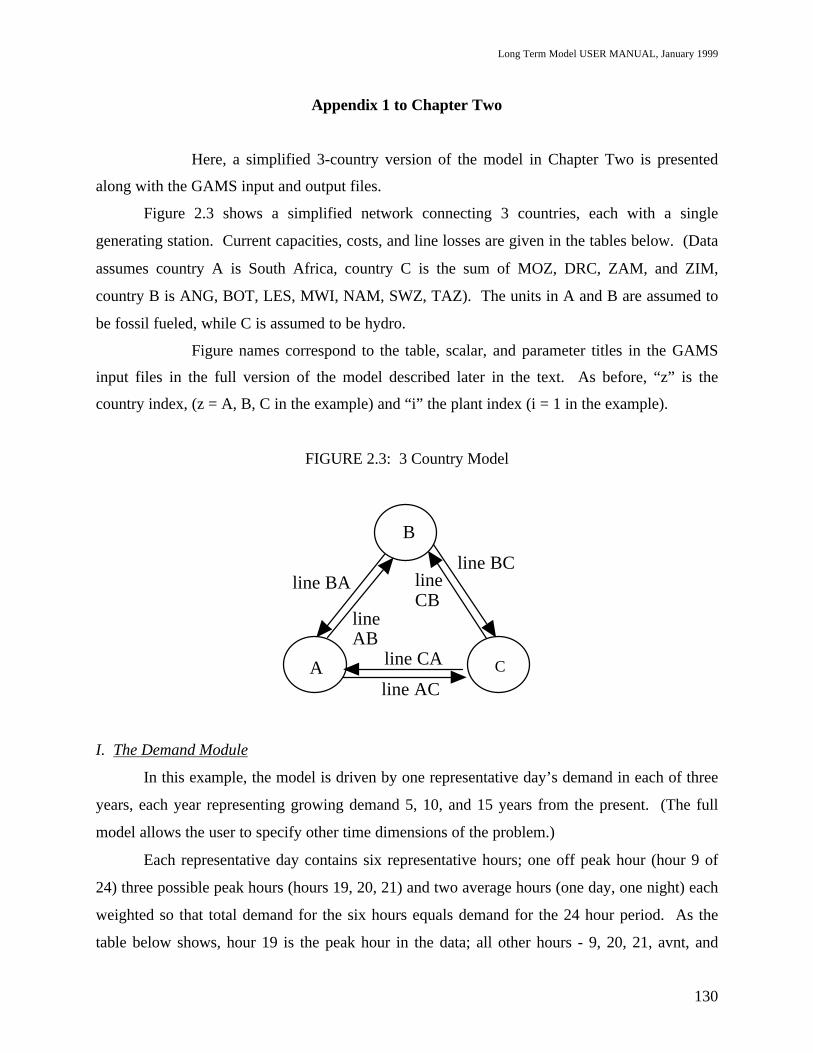
Long Term Model USER MANUAL, January 1999
130
Appendix 1 to Chapter Two
Here, a simplified 3-country version of the model in Chapter Two is presented
along with the GAMS input and output files.
Figure 2.3 shows a simplified network connecting 3 countries, each with a single
generating station. Current capacities, costs, and line losses are given in the tables below. (Data
assumes country A is South Africa, country C is the sum of MOZ, DRC, ZAM, and ZIM,
country B is ANG, BOT, LES, MWI, NAM, SWZ, TAZ). The units in A and B are assumed to
be fossil fueled, while C is assumed to be hydro.
Figure names correspond to the table, scalar, and parameter titles in the GAMS
input files in the full version of the model described later in the text. As before, “z” is the
country index, (z = A, B, C in the example) and “i” the plant index (i = 1 in the example).
FIGURE 2.3: 3 Country Model
B
CA
line BA
line AB
line CA
line AC
line BCline CB
I. The Demand Module
In this example, the model is driven by one representative day’s demand in each of three
years, each year representing growing demand 5, 10, and 15 years from the present. (The full
model allows the user to specify other time dimensions of the problem.)
Each representative day contains six representative hours; one off peak hour (hour 9 of
24) three possible peak hours (hours 19, 20, 21) and two average hours (one day, one night) each
weighted so that total demand for the six hours equals demand for the 24 hour period. As the
table below shows, hour 19 is the peak hour in the data; all other hours - 9, 20, 21, avnt, and

Long Term Model USER MANUAL, January 1999
131
avday - are considered off peak. (Again the full model allows demands of up to 24 hours per
day to be specified for each country.)
These demands, along with the growth rates assumed for each country, are given
in the tables below. Growth percentages are for 5-year intervals based on yearly growth for A,
B, and C being 1.036, 1.07, and 1.06, respectively. Domestic loss coefficients are given in Table
“DLC(z)”. No DSM is assumed in the example.
Table: July 24 97 (th,z)
(hourly demand in MW)
Country “z”
weight hour “th” A B C
1 hour 9 26,400 1300 3600
8 avnt 20,600 1000 2700
1 hour 19 27,600 1300 3600
1 hour 20 26,800 1300 3600
1 hour 21 25,800 1300 3500
12 avdy 23,300 1200 3400
Parameter dgrowth(z)
(5 year percentage growth in demand)
A 1.20
B 1.40
C 1.34
Table DLC(z)
(domestic distribution loss)
A 1.10
B 1.05
C 1.08

Long Term Model USER MANUAL, January 1999
132
Transmission line loss for the lines connecting A, B, and C are given in Table “PFloss
(z,zp)”.
from country “z” to country “zp”
A B C
A 0 0.11 0.15
B 0.11 0 0.08
C 0.15 0.08 0
The demand/supply equations for each of the three countries can now be specified for
each of the six hours in each of the three years.
Country A, hour 9, year 1
PG(9,1, A,1) + PF(9,1,B, A)(1 − 0.11) + PF(9,1,C, A)(1 − 0.15) − PF(9,1, A, B)
−PF(9,1, A,C) = (26, 400)(1.1)(1.2)
M
Country C, hour avdy, year 3
PG(avdy, 3,C,1) + PF(avdy,3, A,C)(1 − 0.15) + PF(avdy, 3,B,C)(1 − 0.08)
−PF(avdy,3,C,A) − PF(avdy,3,C,B) = (3400)(1.08)(1.34)3
II. The Capacity Constraint Module
1. Generation
Supply in each country comes initially from a single plant, whose current capacity
is given in Table “PGinit”. Forced and unforced outage rates for the plants per year are given in
Tables “FORPG” and “UFORP”. For simplicity, no decay is assumed to take place.

Long Term Model USER MANUAL, January 1999
133
Table UFORP(z,i)
Country
“z”
Plant “i”
A 0.10
B 0.10
C 0.10
Table FORPG(z,i)
Country
“z”
Plant “i”
A 0.04
B 0.04
C 0.04
Table PG init(z,i) (MW)
Country
“z”
Plant “i”
A 30,000
B 1800
C 9800

Long Term Model USER MANUAL, January 1999
134
Table “expstep(z,i)” gives the MW capacity of each unit added to existing capacity at
each site “i”.
Table expstep(z,i) (MW)
Country
“z”
Plant “i”
A 500
B 300
C 170
Defining “Y(y,z,i)” to be the integer varialbe = 0,1,2,3,etc., indicating how many units
are installed in year “y” in country “z”, we have the following definitions:
PGexp(y,A,1) = 500Y(y,A,1) y = 1,2,3,etc.
PGexp(y,B,1) = 300Y(y.B,1) y = 1,2,3,etc.
PGexp(y,C,1) = 170Y(y,C,1) y = 1,2,3,etc.
Assuming the forced and unforced outage rates apply to old and new units alike at
each plant site, the capacity constraints for peak and off-peak periods can now be constructed:
(2a)
PG(hr19,1,A,1) ≤ (30,000 + 500Y(1, A,1))(1 − 0.04)
M
PG(hr19,3,C,1) ≤ 9,800 + 170Y(1, C,1) + 170Y(2,C,1)[
+170Y(3, C,1)]* (1 − 0.04),
(2b)
PG(offpeak,1, A,1) ≤ (30, 000 + 500Y(1,A,1))(1 − 0.04)(1 − 0.10)
M
PG(offpeak, 3,C,1) ≤ 9,800 + 170Y(1,C,1) + 170Y(2, C,1)[
+170Y(3, C,1)]* (1 − 0.04)(1 − 0.10), offpeak = hr9,20, 21, avnt,avdy

Long Term Model USER MANUAL, January 1999
135
(In the full model, the distinction is made between peak and off-peak days, not hours within the
day, as is done here to minimize time complexity.)
The hydro plant in country C has one additional capacity constraint, if it is assumed to be
a reservoir facility, rather than “run of the river” – that the reservoir cannot be drained. While
the full model has such a constraint in it for each reservoir – that initial volume minus total daily
outflows plus daily inflows must be non-negative-here, we simply assume that the power
generated over the 24 hours in the representative day cannot exceed 24 times the MW capacity
during the year – e.g.,
PG(hr9,y, C,1) + 8PG(avnt, y,C,1) + PG(hr19, y,C,1)
+PG(hr20, y,C,1) + PG(hr21,y,C,1) + 12PG(avdy, y,C,1)
≤ 24 9800 + 170Y(τ, C,1)τ=1
y
∑
for all y
In the full model, the scalar “24” is replaced by a factor which varies, depending on the season -
wet or dry.
2. Transmission
The current capacities of the transmission system in MW are given in the
following table.
Table PFinit(z,zp) (MW)
A B C
A (S.A.) 0 575 2150
B (other) 575 0 350
C (MOZ, ZAM, ZIM, DRC) 2150 350 0
It will be assumed that transmission capacity can be added in 200 MW increments.
Letting “Y(y,z,zp)” be the integer variable giving the number of increments to line capacity
added to line “z,zp” (and “zp,z”) in year “y” we have

Long Term Model USER MANUAL, January 1999
136
PFexp(y,z,zp) = 200Y(y,z,zp)
The forced outage fate for all lines “FOR(z,zp)” is assumed to be the same 0.10
figure. This data can be used to construct the capacity constraints for the transmission lines
connecting A, B, and C.

Long Term Model USER MANUAL, January 1999
137
Lines {AB,BA}
PF(t,1, A, B) ≤ (575 + 200Y(1, A, B)(1 − 0.10)
PF(t,1, B,A) ≤ (575 + 200Y(1, B,A)(1 − 0.10)
Y(1, A,B) = Y(1, B, A)
M
PF(t, 3, B,C) ≤ 350 + 200Y(1, B,C) + 200Y(2, B,C)[
+300Y(3, B, C)](1 − 0.10)
PF(t, 3,C, B) ≤ 350 + 200Y(1, C,B) + 200Y(2,C, B)[
+200Y(3, C,B)](1 − 0.10)
Y(3,B,C) = Y(3,C,B)
III. The Reliability Module
The reliability constraints can be written with the assumption that “RES(i)” = 0.19 for
thermal units, 0.10 for the hydro unit, and 0.25 for net imports:
(4a) Country A:
30,000 + PG exp(1, A,1)
1 + 0.19
+PF(19,1, B, A)(1 − .11) + PF(19,1,C,A)(1 − .15) − PF(19,1, A,B) − PF(19,1,A, C)
1 + 0.25
≥ (27, 600)(1.1)(1.2)
M

Long Term Model USER MANUAL, January 1999
138
Country C:
2,800 + PG exp(1,C,1) + PG exp(2,C,1) + PG exp(3, C,1)
1 + 0.10
+PF(20, 3,B,C)(1 − .08) + PF(20,3, A,C)(1 − .15) − PF(20, 3,C, A) − PF(20, 3,C, B)
1 + 0.25
≥ (3,600)(1.08)(1.34)3
“MaxPG(z)” will be assumed to be 10% of the total capacity for each country: hence in each:
(4b) Country A:
30,000 + PG exp(1, A,1) + PF(19,1, B, A) + PF(19,1,C, A)
−PF(19,1, A,B) − PF(19,1, A,C) ≥ (27, 600)(1.1) + (27, 600)(0.1)
M
Country C: ...
IV. The Country Autonomy Module
Table “AF(z,y)” gives the autonomy factors assumed for each of the countries, to hold
over all hours.
Table AF(z,y)
(autonomy factor)
Country “z” Year “y”
1 2 3
A 0.95 0.9 0.8
B 0.45 0.35 0.3
C 1 1 1
(Since country C will export, “AF(z,y)” is assumed 1.)
Hence the equations are:

Long Term Model USER MANUAL, January 1999
139
Country A
30,000 + PG exp(1, A,1) ≥ (.95)(26, 400)(1.1)(1.2)
M
Country C
9,800 + PG exp(1,C,1) + PG exp(2, C,1) + PG exp(3, C,1)
≥ (1)(3,400)(1.08)(1.34)3
V. The Objective Function Module
1. Operating Costs
Tables “HR(z,i)”, “fp(z,i)” and “fpesc(z,i)” give the heat rates, fuel costs, and fuel
escalation price rates, assumed for old and new plants in countries A, B, and C. (The heat rate
for hydro is scaled to 1 to allow the water charge to be .15/MWh for the hydro facilities in
country C.
Table HR (z,i)
(BTU/KWh) x 103
Country
“z”
Plant “i”
A 9.8
B 7.5
C 1
Table fp(z,i)
($/106 BTU)
Country
“z”
Plant “i”
A 0.40
B 1.00
C 0.15
Table fpesc(z,i)
Country
“z”
Plant “i”
A 1.01
B 1.02
C 1.00
When the heat rates, in BTU/MWh are multiplied by the fuel costs, in $/106 BTU, the resultant
charge is in $/MWh.
Since, in this example, the operating characteristics of new and old plants are assumed
identical, there is no need to distinguish between the operating costs of old and new plants.
In constructing the operating cost term in the objective function, it is important to
properly weight the hours of operation to insure the six representative hours add up to 24 hours

Long Term Model USER MANUAL, January 1999
140
of use. Parameter “Mtod(th)” gives these weights. Since one day is chosen to represent the
whole year, the resultant 24 hour daily costs need to be multiplied by 365:
Parameter Mtod(th)
hr 9 1
avnt 8
hr 19 1
hr 20 1
hr 21 1
avdy 12
The yearly generation cost for year one in country A is yearly generation times year one
cost/MWh, the product of the heat rate times the cost/106 BTU, or (9.8)(0.4) = $3.92/MWh times
the yearly generation.
Thus, yearly generation cost for the plant in country A in year “0” is:
PG(hr9,1,A,1) + 8PG(avnt,1, A,1) + PG(hr19,1,A,1) + PG(hr20,1,A,1)[
+PG(hr21,1, A,1) + 12PG(avdy,1, A,1)] 365[ ] 3.92[ ]
and the present value at time “0” over the 15-year horizon for each of the three representative
years, each representing a 5-year interval, is:
ty=1
3
∑
PG(hr9, ty, A,1) + 8PG(avnt, ty, A,1) + PG(hr19,ty, A,1)[
+PG(hr20, ty, A,1) + PG(hr21, ty, A,1) + 12PG(avdy, ty, A,1)]
(3.92)365 1.01[ ]5ty
(1 + disc)5ty

Long Term Model USER MANUAL, January 1999
141
The discount rate is given in the Table “scalar int”; the normal value is 10%; users can
specify other values.
Similar present value terms for fuel costs can be constructed for countries B and C.
2. New Equipment Costs
Each country’s plant can be expanded in fixed increments during each time
period. “PGexp(y,z,i)” is the amount added to country “z’s” capacity in period “y”.
Characteristics of the plant expansion for each country are given below.
Characteristic Country
A B C
Fixed cost ($ x 106) 580 430 125
Fixed capacity (MW) 500 300 170
(Country A’s plant is a large coal facility, country B a smaller coal plant, and country C added
hydro capacity for the example.) Recalling that “Y(y,z,i)” indicates the number of units added in
year “y”, total investment in year “y” in each country is then (580)Y(y,A,1) for A, (430)Y(y,B,1)
for B, and 125Y(y,C,1) for C.
The capital recovery factors for plants in A and B are assumed to be 0.16 while C, the
hydro facility, having a longer life, is 0.12. The per period charges for new capacity in each
country is then (0.16)(580)Y(y,A,1) for A, (0.16)(430)Y(y,B,1) for B, and (0.12)(125)Y(y,c,1)
for C.
The present value at time “0” of these to the end of the planning horizon, using the
general expression
CRF(r, n)expcost(z, i)Y(τ, z, i)
(1 + disc)yτ=1
y
∑y=1
Y
∑
is then:

Long Term Model USER MANUAL, January 1999
142
Present Value of;
Country
Charges in the first
period
Charges in the second period Charges in the third period
A (.16)(580)Y(1,A,1)
(1.1)5(.16)(580)Y(τ, A,1)
(1.1)10τ=1
2
∑ (.16)(580)Y(τ, A,1)
(1.1)15τ=1
3
∑
B (.16)(430)Y(1, B,1)
(1.1)5(.16)(430)Y(τ, B,1)
(1.1)10τ=1
2
∑(.16)(430)Y(τ, B,1)
(1.1)15τ=1
3
∑
C (.12)(125)Y(1, C,1)
(1.1)5(.12)(125)Y(τ, C,1)
(1.1)10τ=1
2
∑(.12)(125)Y(τ, C,1)
(1.1)15τ=1
3
∑
All that remains is to enter the transmission capacity equation costs into the objective
function. It will be assumed that capacity can be added in 200 MW increments with the cost per
increment according to the following table;:
Table PFOVC (z,zp) ($ x 106)
To
From A B C
A 0 30 300
B 30 0 30
C 300 30 0
In a manner analogous to generation capacity expansion, we have:
PFexp(y,z,zp) = 200Y(y,z,zp) for all y, z, and zp
where Y(y,z,zp) = 0, 1, 2, 3...., and each expansion adds 200 MW to capacity.

Long Term Model USER MANUAL, January 1999
143
Costs of transmission capacity expansion differ depending on the arc -- e.g., the cost per
200 MW expansion for each arc is:
arc AB = 30Y(y,A, B)
2
arc BA = 30Y(y,B,A)
2
arc AC = 300Y(y,A, C)
2
arc CA = 300Y(y,C, A)
2
arc CB = 30Y(y,C, B)
2
arc BC = 30Y(y,B,C)
2
and Y(y,z,zp) = Y(y,zp,z) for all pairs.
The present value of the annual charges from time of installation to the end of the
planning horizon, as in the case of generation expansion, is given in the following table,
assuming a CRF of 12% for all lines:
Present value of;
Arc Charges in first period Charges in second period Charges in third period
A,B (.12)(30)Y(1,A, B)
(2)(1.1)5(.12)(30)Y(τ, A,B)
(2)(1.1)10τ=1
2
∑(.12)(30)Y(τ, A,B)
(2)(1.1)15τ=1
3
∑
B,A (.12)(30)Y(1,B,A)
(2)(1.1)5(.12)(30)Y(τ,B, A)
(2)(1.1)10τ=1
2
∑(.12)(30)Y(τ,B, A)
(2)(1.1)15τ=1
3
∑
M
The full model input file in GAMS format, and the results of the optimization follows.

Long Term Model USER MANUAL, January 1999
144
A) Demand
The model is driven by the “typical hour/day/season/year” chronological demand
approach taken by many of the latest commercial models, rather than the load duration curve
methodology used in earlier approaches.
Each SAPP region enters in “Table 2000 day type td(th,z)”, their 24-hour base year MW
load patterns for 6 day types -- summer peak, off-peak, and average days, and winter peak, off-
peak, and average day patterns. (2000 was chosen as the base to allow for known growth in
demand in the early years.) Depending on the option chosen by the user, the 24-hour pattern
itself, a 6-hour approximation of the 24-hour pattern (consisting of 4 peak and 2 off-peak hours)
or a 1-hour option can be chosen, depending on the nature of the run, and the trade-off in the
user’s mind between accuracy and running time. (The 24-hour model can take several hours to
run, while the 6-hour model usually takes less than 50 minutes without a large reduction in
accuracy.)
Scalar multiples are applied to the representative hours (“parameter Mtod(th1)”) to scale
up the sample hours to represent the demand over each 24-hour period.
Scalar multiples are also applied to each of the three day types in the summer (9 months)
and winter (3 months) seasons (“parameter Mday(td)”) to insure each year has 365 demand days.
Seven representative years are chosen to model demand growth over the model’s 20-year
planning horizon. Since greater timing detail is needed in the first 10 years than the second,
every other year is modeled for the first 10 years; thereafter every fifth year is represented for a
total of seven years over the 20-year horizon. Yearly demand growth rates which differ by day
type, by time period, and by country (“parameter dgrowth1(z,td)”, to “dgrowth6(z,td)” in the
model) are specified by the user. The program automatically converts the yearly growth rates
into the proper growth rates for the 2- and 5-year intervals between years.
In order to more accurately capture the spatial location of both generation and
consumption points in the model, as well as reflect the realities of the existing/proposed
transmission system, the Republic of South Africa, Mozambique, and the Democratic Republic
of the Congo are represented by two demand nodes each rather than one.
Two other terms appear in the model in association with demand – the Domestic Loss
Coefficient and Demand-Side Management. The domestic loss coefficient – (“parameter
“DLC(z)”) in the model – is applied to the demand value to allow for electricity loss within each

Long Term Model USER MANUAL, January 1999
145
SAPP region. Thus, it converts demand at the customer meter into demand at the generating
station.
The demand-side management (DSM) parameter – (“LM(th,z)” in the model) – allows
SAPP member specified DSM options to fractionally adjust up or down the load shapes of the
representative days in the model, with user-specified costs of such programs entered into the
objective function. It should be emphasized that the model does not compete DSM against
normal supply side options to obtain the least cost mix of DSM and capacity expansion. It
simply allows various DSM options with known costs and benefits to be entered into the model
to see “off-line” if they are cost effective.
The upshot of all this is the specification of the right-hand side of the load balance
equation, which specifies: for each hour in each day in each season in each year, the demand at
the generating station that must be met inclusive of the effect of distribution line loss and DSM
programs. Letting Dyr(ty,ts,td,th,z) be the country z’s MW demand during hour “th” of day type
“td” in season “ts” during year ty, we have:
Dyr(ty, ts, td, th, z) = 2000 Daytype " td"(th,z) 1 + dgrowth(td, z)( )ty
and total demand in country z to be met at the generating stations in the interval {ty,ts,td,th} is
then:
Dyr(ty, ts, td, th, z)(DLC(z)) − DSM(th,z)

Long Term Model USER MANUAL, January 1999
146
Appendix 1A to Chapter 4 Data Tables(The Demand for Electricity)
(data file, section 2)parameter dgrowth2(z) {demand growth rate for period 2}/Ang 1.079 This is where users enter the annual growth rates bycountry. Bot 1.043 Default rates from Peter Robinson’s projections given at Les 1.061 July 98 Cape Town workshop Mwi 1.032 NMz 1.108 SMz 1.109 Nam 1.072 NSA 1.036 SSA 1.036 Swz 1.034 Taz 1.060 DRC 1.050 Zam 1.044 Zim 1.041/;
(data file, section 3)parameter dgrowth3(z) {demand growth rate for period 3}/Ang 1.079 Bot 1.043 Les 1.061 Mwi 1.032 NMz 1.108 SMz 1.109 Nam 1.072 NSA 1.036 SSA 1.036 Swz 1.034 Taz 1.060 DRC 1.050 Zam 1.044 Zim 1.041/;
(data file, section 4)parameter dgrowth4(z) {demand growth rate for period 4}/Ang 1.079 Bot 1.043 Les 1.061 Mwi 1.032 NMz 1.108 SMz 1.109 Nam 1.072 NSA 1.036 SSA 1.036 Swz 1.034 Taz 1.060 DRC 1.050 Zam 1.044 Zim 1.041/;

Long Term Model USER MANUAL, January 1999
147
(data file, section 4)parameter dgrowth5(z) {demand growth rate for period 5}/Ang 1.079 Bot 1.043 Les 1.061 Mwi 1.032 NMz 1.108 SMz 1.109 Nam 1.072 NSA 1.036 SSA 1.036 Swz 1.034 Taz 1.060 DRC 1.050 Zam 1.044 Zim 1.041
/;
(gms. file, section 1)scalar n number of years in each time interval / 5 /;
parameter Mperiod(ty) multiplier of year;Mperiod(ty) = n;
Parameter dgr(z,ty); dgr(z,'yr2') = power (dgrowth2(z),2*n); dgr(z,'yr3') = power (dgrowth2(z),2*n) * power (dgrowth3(z),n); dgr(z,'yr4') = power (dgrowth2(z),2*n) * power (dgrowth3(z),n) * power(dgrowth4(z),n); dgr(z,'yr5') = power (dgrowth2(z),2*n) * power (dgrowth3(z),n) * power(dgrowth4(z),n) * power (dgrowth5(z),n);
parameter HA(ty);HA(ty) = n*(1+ord(ty));
Parameter DW; DW = n;
*=== sapp98model/demand.inc ====
******************************* Section 1***********************************
* This is the demand for year 2000!
****************************************************************** Be sure change july2497(th,z) and PeakD(ty,z) ******************************************************************
$ontext*-------------------- One hour demand data -----------------------SET th Hours index / hr19 /;scalar thT number of hours in a day /1/;

Long Term Model USER MANUAL, January 1999
148
Table PeakD(ty,z) Ang Bot Les Mwi NMz SMz Nam NSA SSA Swz Taz DRC Zam Zimyr1 215 208 66 185 53 101 271 22287 5309 118 416 618 1025 1885;
Table july2497(th,z) Hourly System load on July 24 1997Ang Bot Les Mwi NMz SMz Nam
hr19 215 208 66 185 53 101 271
+ NSA SSA Swz Taz DRC Zam Zimhr19 22287 5309 118 416 618 1025 1885;$offtext
******************************* Section 2***********************************
*--------------------- Six hour demand data ----------------------- {weights}
scalar thT number of hours in a day /6/;
Parameter Mtod(th) /hr9 1avnt 8hr19 1hr20 1hr21 1avdy 12 / ;
Table PeakD(ty,z) {peak demand for each region in each year} Ang Bot Les Mwi NMz SMz Nam NSA SSA Swz Taz DRC Zam Zimyr2 215 211 74 156.4 81 101 296 22287 5309 118 416 721 1062 1885;
******************************* Section 3***********************************
Table july2400(ts,td,th,z) Hourly System load on July 24 1997
Ang Bot Les Mwi NMz SMz Namwinter.peak.hr9 215 211 74 144 81 70 286winter.peak.avnt 185 149 45 101.7 47 61 204winter.peak.hr19 214 189 66 156.4 53 101 271winter.peak.hr20 215 191 71 137.5 69 95 298winter.peak.hr21 214 189 66 123.5 64 91 296winter.peak.avdy 200 185 60 133.1 73 72 270
winter.average. hr9 172 168.8 59.2 115.2 64.8 56 228.8winter.average. avnt 148 119.2 36 81.36 37.6 48.8 163.2winter.average. hr19 171 151.2 52.8 125.12 42.4 80.8 216.8winter.average. hr20 172 152.8 56.8 110 55.2 76 238.4winter.average. hr21 171 151.2 52.8 98.8 51.2 72.8 236.8winter.average. avdy 160 148 48 106.48 58.4 57.6 216
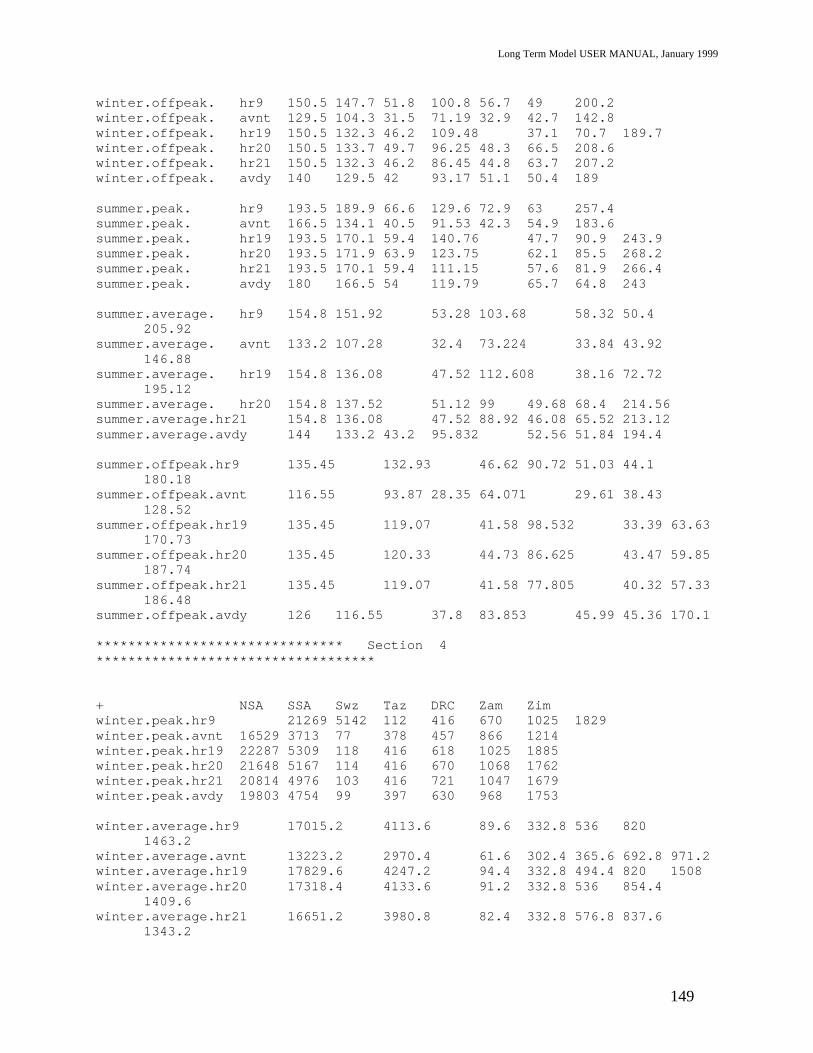
Long Term Model USER MANUAL, January 1999
149
winter.offpeak. hr9 150.5 147.7 51.8 100.8 56.7 49 200.2winter.offpeak. avnt 129.5 104.3 31.5 71.19 32.9 42.7 142.8winter.offpeak. hr19 150.5 132.3 46.2 109.48 37.1 70.7 189.7winter.offpeak. hr20 150.5 133.7 49.7 96.25 48.3 66.5 208.6winter.offpeak. hr21 150.5 132.3 46.2 86.45 44.8 63.7 207.2winter.offpeak. avdy 140 129.5 42 93.17 51.1 50.4 189
summer.peak. hr9 193.5 189.9 66.6 129.6 72.9 63 257.4summer.peak. avnt 166.5 134.1 40.5 91.53 42.3 54.9 183.6summer.peak. hr19 193.5 170.1 59.4 140.76 47.7 90.9 243.9summer.peak. hr20 193.5 171.9 63.9 123.75 62.1 85.5 268.2summer.peak. hr21 193.5 170.1 59.4 111.15 57.6 81.9 266.4summer.peak. avdy 180 166.5 54 119.79 65.7 64.8 243
summer.average. hr9 154.8 151.92 53.28 103.68 58.32 50.4205.92
summer.average. avnt 133.2 107.28 32.4 73.224 33.84 43.92146.88
summer.average. hr19 154.8 136.08 47.52 112.608 38.16 72.72195.12
summer.average. hr20 154.8 137.52 51.12 99 49.68 68.4 214.56summer.average.hr21 154.8 136.08 47.52 88.92 46.08 65.52 213.12summer.average.avdy 144 133.2 43.2 95.832 52.56 51.84 194.4
summer.offpeak.hr9 135.45 132.93 46.62 90.72 51.03 44.1180.18
summer.offpeak.avnt 116.55 93.87 28.35 64.071 29.61 38.43128.52
summer.offpeak.hr19 135.45 119.07 41.58 98.532 33.39 63.63170.73
summer.offpeak.hr20 135.45 120.33 44.73 86.625 43.47 59.85187.74
summer.offpeak.hr21 135.45 119.07 41.58 77.805 40.32 57.33186.48
summer.offpeak.avdy 126 116.55 37.8 83.853 45.99 45.36 170.1
******************************* Section 4***********************************
+ NSA SSA Swz Taz DRC Zam Zimwinter.peak.hr9 21269 5142 112 416 670 1025 1829winter.peak.avnt 16529 3713 77 378 457 866 1214winter.peak.hr19 22287 5309 118 416 618 1025 1885winter.peak.hr20 21648 5167 114 416 670 1068 1762winter.peak.hr21 20814 4976 103 416 721 1047 1679winter.peak.avdy 19803 4754 99 397 630 968 1753
winter.average.hr9 17015.2 4113.6 89.6 332.8 536 8201463.2
winter.average.avnt 13223.2 2970.4 61.6 302.4 365.6 692.8 971.2winter.average.hr19 17829.6 4247.2 94.4 332.8 494.4 820 1508winter.average.hr20 17318.4 4133.6 91.2 332.8 536 854.4
1409.6winter.average.hr21 16651.2 3980.8 82.4 332.8 576.8 837.6
1343.2

Long Term Model USER MANUAL, January 1999
150
winter.average.avdy 15842.4 3803.2 79.2 317.6 504 774.41402.4
winter.offpeak.hr9 14888.3 3599.4 78.4 291.2 469 717.51280.3
winter.offpeak.avnt 11570.3 2599.1 53.9 264.6 319.9 606.2 849.8winter.offpeak.hr19 15600.9 3716.3 82.6 291.2 432.6 717.5
1319.5winter.offpeak.hr20 15153.6 3616.9 79.8 291.2 469 747.6
1233.4winter.offpeak.hr21 14569.8 3483.2 72.1 291.2 504.7 732.9
1175.3winter.offpeak.avdy 13862.1 3327.8 69.3 277.9 441 677.6
1227.1
summer.peak.hr9 19142.1 4627.8 100.8 374.4 603 922.51646.1
summer.peak.avnt 14876.1 3341.7 69.3 340.2 411.3 779.4 1092.6summer.peak.hr19 20058.3 4778.1 106.2 374.4 556.2 922.5 1696.5summer.peak.hr20 19483.2 4650.3 102.6 374.4 603 961.2 1585.8summer.peak.hr21 18732.6 4478.4 92.7 374.4 648.9 942.3 1511.1summer.peak.avdy 17822.7 4278.6 89.1 357.3 567 871.2 1577.7
summer.average.hr9 15313 3702.24 80.64 299.52 482.4 7381316.88
summer.average.avnt 11900 2673.36 55.44 272.16 329.04623.52 874.08
summer.average.hr19 16046 3822.48 84.96 299.52 444.96 7381357.2
summer.average.hr20 15586 3720.24 82.08 299.52 482.4 768.961268.64
summer.average.hr21 14986 3582.72 74.16 299.52 519.12753.84 1208.88
summer.average.avdy 14258 3422.88 71.28 285.84 453.6 696.961262.16
summer.offpeak.hr9 13399 3239.46 70.56 262.08 422.1 645.751152.27
summer.offpeak.avnt 10413 2339.19 48.51 238.14 287.91545.58 764.82
summer.offpeak.hr19 14040 3344.67 74.34 262.08 389.34645.75 1187.55
summer.offpeak.hr20 13638 3255.21 71.82 262.08 422.1 672.841110.06
summer.offpeak.hr21 13112 3134.88 64.89 262.08 454.23659.61 1057.77
summer.offpeak.avdy 12475 2995.02 62.37 250.11 396.9 609.841104.39
;
$ontext

Long Term Model USER MANUAL, January 1999
151
******************************* Section 5***********************************
*--------------------- 24 hour demand data -----------------------SET
th Hours index / hr1*hr24/;scalar thT number of hours in a day /24/;
Table PeakD(ty,z) {peak demand for each region in each year} Ang Bot Les Mwi NMz SMz Nam NSA SSA Swz Taz DRC Zam Zimyr1 215 209 74 185 85 101 298 22287 5309 118 416 721 1068 1885;
******************************* Section 6***********************************
Table july2497(th,z) Hourly System load on July 24 1997** OK cooked ** ** cooked 0 0 0
Ang Bot Les Mwi NMz SMz Namhr1 185 136 43 148 35 65 205hr2 185 137 42 148 33 60 185hr3 185 138 41 148 39 57 183hr4 185 141 40 148 47 56 183hr5 185 144 40 148 52 56 186hr6 185 156 43 148 57 56 195hr7 215 176 48 148 60 61 217hr8 215 193 62 185 77 65 266hr9 215 211 74 185 81 70 286hr10 215 209 71 185 78 76 292hr11 215 201 68 185 80 76 288hr12 215 202 63 185 85 76 278hr13 185 189 64 148 71 75 276hr14 185 180 59 148 70 71 263hr15 185 177 57 148 76 67 268hr16 185 176 56 148 76 66 271hr17 185 170 56 148 75 66 274hr18 185 167 56 148 64 76 266hr19 215 189 66 185 53 101 271hr20 215 191 71 185 69 95 298hr21 215 189 66 185 64 91 296hr22 215 181 61 148 58 85 282hr23 185 174 57 148 59 72 253hr24 185 169 50 148 57 64 238
******************************* Section 7***********************************
* OK ** ** ** cooked 0 ** **+ NSA SSA Swz Taz DRC Zam Zimhr1 16246 3667 71 378 412 844 1150hr2 16011 3534 70 378 433 855 1137hr3 15901 3501 71 378 453 855 1134hr4 15853 3474 72 378 453 855 1149hr5 16077 3523 76 378 464 887 1224hr6 17493 3863 96 378 464 897 1389

Long Term Model USER MANUAL, January 1999
152
hr7 20087 4597 114 416 618 961 1617hr8 21387 5143 114 416 644 983 1753hr9 21269 5142 112 416 670 1025 1829hr10 20756 4985 102 416 670 1004 1841hr11 20233 4874 102 378 675 972 1825hr12 19737 4741 101 378 675 961 1792hr13 19322 4690 97 378 675 983 1787hr14 19083 4617 93 378 670 940 1729hr15 18887 4614 83 378 618 940 1730hr16 18933 4637 88 378 567 940 1766hr17 19214 4682 90 416 515 951 1799hr18 20642 4933 112 416 567 961 1880hr19 22287 5309 118 416 618 1025 1885hr20 21618 5167 114 416 670 1068 1762hr21 20814 4976 103 416 721 1047 1679hr22 19349 4532 95 416 670 1015 1512hr23 17862 4224 84 378 567 887 1334hr24 16789 3918 77 378 412 844 1194;
******************************* Section 8***********************************
$offtext
(data file, section 5)Parameter DLC(z) {domestic loss coefficient for each region}/Ang 1.05 Bot 1.00 Les 1.05 Mwi 1.05 NMz 1.05 SMz 1.05 Nam 1.05 NSA 1.05 SSA 1.05 Swz 1.05 Taz 1.05 DRC 1.05 Zam 1.05 Zim 1.05 /;
(reserve file, section 12)Table LM(z,th)
hr9 avnt hr19 hr20 hr21 avdyAng 0 0 0 0 0 0Bot 0Les 0Mwi 0NMz 0SMz 0Nam 0NSA 0SSA 0Swz 0Taz 0

Long Term Model USER MANUAL, January 1999
153
DRC 0Zam 0Zim 0;
(lines file, section 3)Table PFOloss(z,zp) {International transmission losscoefficient} Bot Les Mwi Nmz Smz Nam NSA SSA Swz Taz DRC ZamZimBot 0 0 0 0 0 0 0.035 0 0 0 0 00.035Les 0 0 0 0 0 0 0.05 0 0 0 0 00Mwi 0 0 0 0 0 0 0 0 0 0 0 00Nmz 0 0 0 0 0.9 0 0.10 0 0 0 0 00.03Smz 0 0 0 0.9 0 0 0.03 0 0.015 0 0 00Nam 0 0 0 0 0 0 0 0.07 0 0 0 00NSA 0.035 0.05 0 0.10 0.03 0 0 0.03 0.02 0 0 00SSA 0 0 0 0 0 0.07 0.03 0 0 0 0 00Swz 0 0 0 0 0.015 0 0.02 0 0 0 0 00Taz 0 0 0 0 0 0 0 0 0 0 0 0.060DRC 0 0 0 0 0 0 0 0 0 0 0 0.010Zam 0 0 0 0 0 0 0 0 0 0.06 0.01 00.0Zim 0.035 0 0 0.03 0 0 0 0 0 0 0 0.00* Updated at SAPP workshop Capetown [July 06]
(lines file, section 5)Table PFNloss(z,zp) {transmission loss factor [0-1]} Ang Bot Mwi Les Nmz Smz Nam NSA SSA Swz Taz DRC Zam ZimAng 0 0 0 0 0 0 0.14 0 0 0 0 0.02 0 0Bot 0 0 0 0 0 0 0 0 0 0 0 0 0 0Les 0 0 0 0 0 0 0 0 0 0 0 0 0 0Mwi 0 0 0 0 0.03 0 0 0 0 0 0 0 0.04 0Nmz 0 0 0.03 0 0 0.10 0 0 0 0 0 0 0 0Smz 0 0 0 0 0.10 0 0 0 0 0 0 0 0 0Nam 0.14 0 0 0 0 0 0 0 0.02 0 0 0 0 0NSA 0 0 0 0 0 0 0 0 0 0 0 0 0 0SSA 0 0 0 0 0 0 0.02 0 0 0 0 0 0 0Swz 0 0 0 0 0 0 0 0 0 0 0 0 0 0Taz 0 0 0 0 0 0 0 0 0 0 0 0 0 0DRC 0.02 0 0 0 0 0 0 0 0 0 0 0 0.01 0Zam 0 0 0.04 0 0 0 0 0 0 0 0 0.01 0 0Zim 0 0 0 0 0 0 0 0 0 0 0 0 0 0* DRC-ANG-NAM, NMZ-SMZ need to be updated

Long Term Model USER MANUAL, January 1999
154
(hydro file, section 9)Parameter PSOloss; PSOloss = 0.3;
(hydro file, section 9)Parameter PSNloss(phn); PSNloss(phn) = 0.3;

Long Term Model USER MANUAL, January 1999
155
Appendix 1B to Chapter 4 - Adding DSM
At the present time, the model only allows pre-specified levels of “DSM” programs to
enter the problem as an aggregate subtraction from the hourly demand drivers of the model. The
user can then experiment with the impact various pre-specified mixes of “DSM” programs can
have on the cost of SAPP generation, and compare such cost reductions with the increased costs
of implementing the various mixes of programs to see which are cost-effective.
The model could be easily modified to explicitly trade off “DSM” programs against
supply side programs to produce a true least cost SAPP plan in the following way.
Step 1: Identify the range of “DSM” projects which are possible for SAPP members to
implement in sufficient detail to allow comparison with comparable supply side programs.
example: “Replace all motors over 10 HP in RSA with hi∈ motors: result: reduce
all hourly demands by 400 MW; program cost of 400 million dollars (cash rebates to hi∈ motor
purchasers)”
Step 2: Define a “DSM” program level variable bounded between 0 and 1, which allows full
or partial implementation of the project.
example: let “HI∈MOT” be the decision variable for the motor replacement
program described above - 0 ≤ HI∈MOT≤1, i.e., when “HI∈MOT” = .5, cost is (400 x 106)(.5),
MW reduction is (400 MW)(.5).
Step 3: Create the relationship between base demand in hour “i”, the levels chosen for the
“DSM” programs identified, and actual demand in hour “i”
example: actual demand in hour “i” would equal Base Demand without “DSM”
program in “i” minus (HI∈Mot)(400). e.g., if the hi∈ motor plan is fully implemented,
[“HI∈MOT = 1”] then actual demand is Base demand in “i” - 400 MW for all “i”; if half
is implemented, [“HI∈MOT = .5”] actual demand is Base demand in “i” - 200 MW, etc...

Long Term Model USER MANUAL, January 1999
156
Step 4: Enter the levelized cost of the “DSM” program in the objective function;
example: (400 × 10 6 )(HI ∈MOT)(crf )
A general “stand alone” version of the trade off between demand and supply side options
can be formulated in the following way. If “xj” is the decision variable, 0 ≤ xj ≤ 1, which
indicates what fraction of program “j” will be undertaken, “$ j” the cost of the program if “j”
fully undertaken (“xj” = 1), “a τj” the reduction in demand in hour “τ” of a representative day in a
given year if program “j” were fully undertaken (“xj” = 1), “Dyr(τ)” the base demand in hour
“τ” in that representative day, without any DSM (“xj” = 0 for all “j”) “Dyr(τ)” the remaining
portion of the demand met by generation during hour “τ” of the representative day after “DSM”,
“c (τ)” the generation cost/MW of meeting demand by generation in hour “τ”, in that day and K
is scalar which scales up the typical day into a year, the problem of determining the least cost
mix of generation and DSM in that year which satisfies final demand can be stated as:
minx j,Dyr(τ)
(crfj=1
n∑ )($ j )x j + Kc
τ=1
24∑ (τ)Dyr(τ)
sit. Dyr(τ) +j=1
n
∑ a τj x j = Dyr(τ), = 1, 2, ...24
0 ≤ x j ≤ 1 or x j =1
0
The above “stand alone” model is a static model with regards to years - it says what the
options are this year to implement “DSM” programs, what is the impact this year on costs
(through the levelized capital cost) and this year on demands of actions taken this year.

Long Term Model USER MANUAL, January 1999
157
The model can be made dynamic in the following way;
• Allow “xj(ty)” to be the fraction of DSM program “xj” implemented in year “ty”.
Then it must be true that:
x j (ty)ty=1
T
∑ ≤ 1, x j ( ty) ≥ 0 or x j( ty) =1
0
e.g. no more than the full program can be implemented over the planning horizon “T”.
• Letting “Dyr(τ,ty)” be demand met by DSM in hour “τ” in the representative day
in year “ty”, and “Dyr(τ, ty)” be demand in {“τ,ty”} without any “DSM”, the load
balance equation in year “ty” becomes;
Dyr(τ, ty) + a τjj=1
n
∑ x jα=1
ty
∑ (α) = Dyr(τ, ty)
τ = 1,2, ...24
ty = 1,2, ...T
e.g. demand in “ty” in hour “τ” is reduced by the sum effect of all “DSM” programs
implemented up to the year ‘ty”, given by x jα=1
ty∑ (α) .
The objective function becomes;
(crf )($ j )x j ( ty)
(1 + disc) tyatya=ty
T
∑
ty=1
T
∑j=1
n
∑ +Kc(τ, ty)Dyr(τ, ty)
(1 + disc) ty
τ=1
24
∑
The first term inside the bracket is the present value of the stream of levelized capital
charges arising from “DSM” program “xj” in year “ty” and continuing to the end of the horizon.
The second is the cost of satisfying residual demand by generation in year “ty”. The terms in
brackets need to be summed over all “ty”, and also over all “n” “DSM” programs.

Long Term Model USER MANUAL, January 1999
158
The “stand alone” model can be incorporated into the full model by simply entering the
expression
a τjj=1
n
∑ x j (α)α=1
ty
∑
on the supply side of the demand equation as an alternative to the demand side options, and
entering
ty=1
T
∑j=1
n
∑(crf )($ j )x j (ty)
(1 + disc) tyatya=ty
T
∑
in the objective function, and let the model decide on the best mix of demand and supply sideoptions.

Long Term Model USER MANUAL, January 1999
159
Appendix 2 to Chapter 4(Capacity Constraint Module)
Old Thermal Tables, Section 2a
(thermal file, section 13)Table PGOinit(z,i) current capacity for old thermo plants
Stat1 Stat2 Stat3 Stat4 Stat5 Stat6Ang 114Bot 118Les 1.8Mwi 0NMz 12SMz 0Nam 108 24NSA 3510 1320 3450 1900 3840 2700SSA 1840Swz 9Taz 112DRC 37Zam 80Zim 956 80 70 120
+ Stat7 Stat8 Stat9 Stat10NSA 3558 1836 3690 3450
(thermal file, section 4)
Table PGOexpstep(z,i) expansion step size for old thermo plants units Stat1 Stat2 Stat3 Stat4 Stat5 Stat6Ang 50Bot 25Les 0.4Mwi 4NMz 3SMz 15Nam 25 6NSA 850 320 850 450 950 650SSA 450Swz 2Taz 45DRC 0Zam 20Zim 240 20 15 30
+ Stat7 Stat8 Stat9 Stat10NSA 850 450 900 850
(thermal file, section 14)Table PGOmax(z,i) max possible MW addition to old thermo plants Stat1 Stat2 Stat3 Stat4 Stat5 Stat6Ang 0Bot 0Les 0Mwi 0NMz 0SMz 0

Long Term Model USER MANUAL, January 1999
160
Nam 0NSA 0SSA 0Swz 0Taz 0DRC 0Zam 0Zim 0
+ Stat7 Stat8 Stat9 Stat10NSA 0;
(gms file, section 2)Scalar DecayPGO decay rate of old thermo /0.001/;
(reserve file, section 2)Table FORPGO(z,i) {force outage rate for old thermo units}
Stat1 Stat2 Stat3 Stat4 Stat5 Stat6Ang 0.04Bot 0.04Les 0.04Mwi 0.04NMz 0.04SMz 0.04Nam 0.04 0.04NSA 0.04 0.04 0.04 0.04 0.04 0.04SSA 0.04Swz 0.04Taz 0.04DRC 0.04Zam 0.04Zim 0.04 0.04 0.04 0.04
+ Stat7 Stat8 Stat9 Stat10NSA 0.04 0.04 0.04 0.04;
(reserve file, section 10)Table UFORPGO(z,i) {unforce outage rate for old thermo plants} Stat1 Stat2 Stat3 Stat4 Stat5 Stat6Ang 0.10Bot 0.10Les 0.10Mwi 0.10NMz 0.10SMz 0.10Nam 0.10 0.10NSA 0.10 0.10 0.10 0.10 0.10 0.10SSA 0.10Swz 0.10Taz 0.10DRC 0.10Zam 0.10Zim 0.10 0.10 0.10 0.10
+ Stat7 Stat8 Stat9 Stat10

Long Term Model USER MANUAL, January 1999
161
NSA 0.10 0.10 0.10 0.10;
Old Hydro Tables, Section 2b
(hydro file, section 4)Table HOinit(z,ih) {Existing hydro initial capacity (MW)} Stat1 Stat2 Stat3 Stat4 Stat5Ang 121 56 37.3 37.3 37.3Les 24Mwi 214NMz 2075 81SMz 16.6Nam 240NSA 400 1000SSA 320 220Swz 20 15 6.5DRC 1775 248 108 68.04 42Taz 204 80 66 21 8Zam 600 900 100Zim 666;
(hydro file, section 5)Table HOexpstep(z,ih) expansion step for existing hydro {HOVmax/5}
Stat1 Stat2 Stat3 Stat4 Stat5Ang 45 {Cambambe Extension}NMz 1240 {Cahorra Bassa Extension}Zam 150 {Kariba North Extension, only if Batoka}Zim 150 {Kariba South Extension, only if Batoka};
(hydro file, section 4)Table HOVmax(z,ih) Max possible expansion on existing hydro
Stat1 Stat2 Stat3 Stat4 Stat5Ang 90 {Cambambe Extension}NMz 1240 {Cahorra Bassa Extension}Zam 300 {Kariba North Extension, only if Batoka}Zim 300 {Kariba South Extension, only if Batoka};
(gms file, section 2)Scalar DecayHO decay rate of old hydro /0.001/;
(hydro file, section 8)Table FORoh(z,ih) {Existing hydro forced outage rate}
Stat1 Stat2 Stat3 Stat4 Stat5Ang 0.028 0.028 0.028Mwi 0.028NMz 0.028 0.028Nam 0.028SSA 0.028 0.028Swz 0.028DRC 0.028 0.028 0.028 0.028 0.028Taz 0.028 0.028Zam 0.028 0.028 0.028Zim 0.028

Long Term Model USER MANUAL, January 1999
162
***----------- Energy (MWh) limit for new hydros ------------- --------------
(hydro file, section 5)Parameter HROmwh(ts,z,ih); {Seasonal MWh cap of existing Run of River}HROmwh(ts,z,ih) = HOinit(z,ih)*(tdT*thT);
*@@@ Old Dams MWh capacity multiplier @@@@ [Zyu june 1 '98] @@@@@@@@@@@@@Parameter fdamO(z,ih,ts);fdamO(z,ih,ts)$(ord(ts) EQ 1) = 1.6; {summer season all ROR hydros}fdamO(z,ih,ts)$(ord(ts) EQ 2) = 0.3; {winter season}
fdamO('Nmz','stat1','summer') = 1.8; {Cahorra Bassa existing}fdamO('Nmz','stat1','winter') = 0.8;
fdamO('DRC','stat1','summer') = 20; {Inga existing}fdamO('DRC','stat1','winter') = 12;
parameter fdrought(ty) (uncertain file) {reduced water flow during drought; 1 = normal <1 is
dry}/yr2 1 yr3 1 yr4 1 yr5 1/;
New Thermal Tables, Section 2c
Combustion Turbines
(thermal file, section 5)Table NTexpstep(z,ni) {expansion step size for new gas turbine plants} NS1 NS2 NS3Ang 50 50 50Bot 50 50 50Les 50 50 50SMz 50 50 50Nam 50 50 50NSA 250 50 50SSA 50 50 50Taz 40 10 50Zim 50 50 50;
(thermal file, section 14)Table PGNTmax(z,ni) NS1 NS2 NS3Ang 450 450 450Bot 450 450 450Les 450 450 450Mwi 450 450 450NMz 450 450 450SMz 450 450 450Nam 450 450 450NSA 1000 450 450SSA 450 450 450Swz 450 450 450

Long Term Model USER MANUAL, January 1999
163
Taz 40 100 450DRC 450 450 450Zam 450 450 450Zim 450 450 450
(gms file, section 2)Scalar DecayNT decay rate of gas turbine /0.001/;
(reserve file, section 2)Table FORNT(ty,z,ni)
NS1 NS2 NS3Ang 0.104 0.104 0.104Bot 0.104 0.104 0.104Les 0.104 0.104 0.104Mwi 0.104 0.104 0.104NMz 0.104 0.104 0.104SMz 0.104 0.104 0.104Nam 0.104 0.104 0.104NSA 0.104 0.104 0.104SSA 0.104 0.104 0.104Swz 0.104 0.104 0.104Taz 0.104 0.104 0.104DRC 0.104 0.104 0.104Zam 0.104 0.104 0.104Zim 0.104 0.104 0.104;
(reserve file, section 5)Table UFORNT(z,ni)
NS1 NS2 NS3Ang 0.07 0.07 0.07Bot 0.07 0.07 0.07Les 0.07 0.07 0.07Mwi 0.07 0.07 0.07NMz 0.07 0.07 0.07SMz 0.07 0.07 0.07Nam 0.07 0.07 0.07NSA 0.07 0.07 0.07SSA 0.07 0.07 0.07Swz 0.07 0.07 0.07Taz 0.07 0.07 0.07DRC 0.07 0.07 0.07Zam 0.07 0.07 0.07Zim 0.07 0.07 0.07;
Small Coal
(thermal file, section 6)Table NSCexpstep(z,ni) {expansion step size for new small coal plants}
NS1 NS2 NS3 NS4 NS5Ang 300 300Bot 120 300Les 300 300SMz 250 300Nam 300 300NSA 90 190 110 190 100

Long Term Model USER MANUAL, January 1999
164
SSA 300 300Taz 300 300Zim 84 300;
(thermal file, section 15)Table PGNSCmax(z,ni) NS1 NS2 NS3 NS4 NS5Ang 600 600Bot 240 600Les 600 600Mwi 600 600NMz 750 600SMz 600 600Nam 600 600NSA 450 1140 440 1520 1000SSA 600 600Swz 600 600Taz 600 600DRC 600 600Zam 600 600Zim 84 600;
(gms file, section 2)Scalar DecayNSC decay rate of small coal /0.001/;
(reserve file, section 4)Table FORNSC(z,ni)
NS1 NS2Ang 0.046 0.046Bot 0.046 0.046Les 0.046 0.046Mwi 0.046 0.046NMz 0.046 0.046SMz 0.046 0.046Nam 0.046 0.046NSA 0.046 0.046SSA 0.046 0.046Swz 0.046 0.046Taz 0.046 0.046DRC 0.046 0.046Zam 0.046 0.046Zim 0.046 0.046;
(reserve file, section 7)Table UFORNSC(z,ni)
NS1 NS2Ang 0.111 0.111Bot 0.111 0.111Les 0.111 0.111Mwi 0.111 0.111NMz 0.111 0.111SMz 0.111 0.111Nam 0.111 0.111NSA 0.111 0.111

Long Term Model USER MANUAL, January 1999
165
SSA 0.111 0.111Swz 0.111 0.111Taz 0.111 0.111DRC 0.111 0.111Zam 0.111 0.111Zim 0.111 0.111;
Combined Cycle
(thermal file, section 1)Table PGNCCinit(z,ni) {initial capacity of new combined-cycleplants} NS1 NS2 NS3Ang 250 250 250Bot 250 250 250Les 250 250 250Mwi 250 250 250NMz 250 250 250SMz 250 250 250Nam 750 250 250NSA 250 250 250SSA 250 250 250Swz 250 250 250Taz 250 250 250DRC 250 250 250Zam 250 250 250Zim 250 250 250
(thermal file, section 5)Table NCCexpstep(z,ni) {expansion step size for combined cycle plantsunits}
NS1 NS2 NS3Ang 250 250 250Bot 250 250 250Les 250 250 250SMz 250 250 250Nam 250 250 250NSA 250 250 250SSA 250 250 250Taz 250 250 250Zim 250 250 250;
(thermal file, section 15)Table PGNCCmax(z,ni)
NS1 NS2 NS3Ang 750 750 750Bot 750 750 750Les 750 750 750Mwi 750 750 750NMz 750 750 750SMz 750 750 750Nam 0 750 750NSA 750 750 750SSA 750 750 750Swz 750 750 750

Long Term Model USER MANUAL, January 1999
166
Taz 750 750 750DRC 750 750 750Zam 750 750 750Zim 750 750 750;
(gms file, section 2)Scalar DecayNCC decay rate of combined cycle /0.001/;
(reserve file, section 3)Table FORNCC(z,ni)
NS1 NS2 NS3Ang 0.104 0.104 0.104Bot 0.104 0.104 0.104Les 0.104 0.104 0.104Mwi 0.104 0.104 0.104NMz 0.104 0.104 0.104SMz 0.104 0.104 0.104Nam 0.104 0.104 0.104NSA 0.104 0.104 0.104SSA 0.104 0.104 0.104Swz 0.104 0.104 0.104Taz 0.104 0.104 0.104DRC 0.104 0.104 0.104Zam 0.104 0.104 0.104Zim 0.104 0.104 0.104;
(reserve file, section 6)Table UFORNCC(z,ni)
NS1 NS2 NS3Ang 0.07 0.07 0.07Bot 0.07 0.07 0.07Les 0.07 0.07 0.07Mwi 0.07 0.07 0.07NMz 0.07 0.07 0.07SMz 0.07 0.07 0.07Nam 0.07 0.07 0.07NSA 0.07 0.07 0.07SSA 0.07 0.07 0.07Swz 0.07 0.07 0.07Taz 0.07 0.07 0.07DRC 0.07 0.07 0.07Zam 0.07 0.07 0.07Zim 0.07 0.07 0.07;
Large Coal(thermal file, section 1)Table PGNLCinit(z,ni) {initial capacity of new lagre coalplants} NS1 NS2 NS3 NS4 NS5 NS6 NS7 NS8Ang 500 500Bot 500 500Les 500 500Mwi 500 500

Long Term Model USER MANUAL, January 1999
167
NMz 500 500SMz 500 500Nam 500 500NSA 659 959 659 659 659 659 659 659SSA 1000 659 659 659Swz 500 500Taz 500 500DRC 500 500Zam 500 500Zim 500 500
(thermal file, section 6)Table NLCexpstep(z,ni) {expansion step size for new large coal plants} NS1 NS2 NS3 NS4 NS5 NS6 NS7 NS8Ang 500 500Bot 500 500Les 500 500SMz 500 500Nam 500 500NSA 659 659 659 659 659 659 659 659SSA 500 500 500 500Taz 500 500Zim 500 500 ;
(thermal file, section 16)Table PGNLCmax(z,ni){max addition to LC} NS1 NS2 NS3 NS4 NS5 NS6 NS7 NS8Ang 4500 4500Bot 4500 4500Les 4500 4500Mwi 4500 4500NMz 4500 4500SMz 4500 4500Nam 4500 4500NSA 3295 3295 3295 3295 3295 3295 3295 3295SSA 4500 3295 3295 3295Swz 4500 4500Taz 4500 4500DRC 4500 4500Zam 4500 4500Zim 4500 4500;
(gms file, section 2)Scalar DecayNLC decay rate of large coal /0.001/;
(reserve file, section 5)Table FORNLC(z,ni)
NS1 NS2 NS3 NS4 NS5 NS6 NS7 NS8Ang 0.047 0.047 0.047Bot 0.047 0.047 0.047Les 0.047 0.047 0.047Mwi 0.047 0.047 0.047NMz 0.047 0.047 0.047SMz 0.047 0.047 0.047Nam 0.047 0.047 0.047

Long Term Model USER MANUAL, January 1999
168
NSA 0.047 0.047 0.047 0.047 0.047 0.047 0.047 0.047SSA 0.047 0.047 0.047Swz 0.047 0.047 0.047Taz 0.047 0.047 0.047DRC 0.047 0.047 0.047Zam 0.047 0.047 0.047Zim 0.047 0.047 0.047;
(reserve file, section 7)Table UFORNLC(z,ni)
NS1 NS2 NS3 NS4 NS5 NS6 NS7 NS8Ang 0.111 0.111Bot 0.111 0.111Les 0.111 0.111Mwi 0.111 0.111NMz 0.111 0.111SMz 0.111 0.111Nam 0.111 0.111NSA 0.111 0.111 0.111 0.111 0.111 0.111 0.111 0.111SSA 0.111 0.111Swz 0.111 0.111Taz 0.111 0.111DRC 0.111 0.111Zam 0.111 0.111Zim 0.111 0.111;
New Hydro Tables
(hydro dile, section 1)set nh new hydro index /newh1*newh4/
Table HNinit(z,nh) Initial MW capacity of New hydro Stations newh1 newh2 newh3 newh4
Ang 130 {CapandaII} 0 0 0Les 0 {Muela } 0 0 0Mwi 32 {Kapichiri I & II} 45 125 {Lower fufu} 35Nmz 400 {Mepandua Uncua } 0 0 0Nam 360 {Epupua/Kunene River } 0 0 0Taz 60 {Lower Kihansi } 74 {Rumakali} 160 {Mpanga} 0DRC 4750 {Grand Inga I & 2} 4750 4750 4750Zam 40 {itezhi-teshi} 150 {Kafue Gorge} 200 {Batoka N} 0
{water: 1260e6 m-cubed/hr }Zim 200 {Batoka S} 300 {Gokwe N} 0 {Kariba} 0
(hydro file, section 3)Table HNexpstep(z,nh) Expansion step for new hydro stations newh1 newh2 newh3 newh4Ang 130 {Capanda}Les 24 {Muela}Mwi 32 {Kapichiri II, Shire} 45 63 35Nmz 400Taz 60 74 89.5DRC 5250 5250 5250 5250Zam 37 150 200

Long Term Model USER MANUAL, January 1999
169
Zim 200 300
(hydro file, section 2)Table HNVmax(z,nh) Max possible MW addition to a new hydro station newh1 newh2 newh3 newh4Ang 130 {Capanda}Les 48 {Muela}Mwi 32 {Kapichiri II, Shire} 45 63 35Nmz 1600Taz 120 148 368.5DRCZam 37 450 600Zim 600 900
(gms file, section 2)Scalar DecayHN decay rate of new hydro /0.001/;
(hydro file, section 8)Table FORnh(z,nh) {forced outage rate for new hydro} newh1 newh2 newh3 newh4Ang 0.028 0.028 0.028 0.028Bot 0.028 0.028 0.028 0.028Les 0.028 0.028 0.028 0.028Mwi 0.028 0.028 0.028 0.028NMz 0.028 0.028 0.028 0.028SMz 0.028 0.028 0.028 0.028Nam 0.028 0.028 0.028 0.028NSA 0.028 0.028 0.028 0.028SSA 0.028 0.028 0.028 0.028Swz 0.028 0.028 0.028 0.028Taz 0.028 0.028 0.028 0.028DRC 0.028 0.028 0.028 0.028Zam 0.028 0.028 0.028 0.028Zim 0.028 0.028 0.028 0.028
***----------- Energy (MWh) limit for new hydros ------------- --------------
(hydro file, section 3)*@@@ New Dams MWh capacity multiplier @@@@ [Zyu june 1 '98] @@@@@@@@@Parameter fdamN(z,nh,ts);fdamN(z,nh,ts)$(ord(ts) EQ 1) = 1.6; {summer season}fdamN(z,nh,ts)$(ord(ts) EQ 2) = 0.3; {winter season}
fdamN('Nmz','newh1',ts)$(ord(ts) EQ 1) = 1.8; {summer season Mapenda Uncua}fdamN('Nmz','newh1',ts)$(ord(ts) EQ 2) = 0.9; {winter season Mapenda Uncua}
fdamN('DRC','newh1',ts)$(ord(ts) EQ 1) = 20; {summer season Inga}fdamN('DRC','newh1',ts)$(ord(ts) EQ 2) = 12; {winter season Inga}
Parameter HDNmwh(z,nh); {annual MWh capacity of new Dam}HDNmwh(z,nh) = HNinit(z,nh)*(tdT*thT)*sum(ts,fdamN(z,nh,ts));
Parameter HRNmwh(ts,z,nh); {Seasonal MWh capacity of new Run of River}HRNmwh(ts,z,nh) = HNinit(z,nh)*(tdT*thT);
(uncertain file)

Long Term Model USER MANUAL, January 1999
170
parameter fdrought(ty) {reduced water flow during drought; 1 = normal <1 isdry}/yr2 1 yr3 1 yr4 1 yr5 1/;
Old Transmission Lines, Section 2e
(lines file, section 1)Table PFOinit(z,zp) Tie line capacities {MW} Ang Bot Les Mwi Nmz Smz Nam NSA SSA Swz Taz DRC Zam ZimAng 0 0 0 0 0 0 0 0 0 0 0 0 0 0Bot 0 0 0 0 0 0 0 850 0 0 0 0 0 650Les 0 0 0 0 0 0 0 130 0 0 0 0 0 0Mwi 0 0 0 0 0 0 0 0 0 0 0 0 0 0Nmz 0 0 0 0 0 0 0 1800 0 0 0 0 0 550Smz 0 0 0 0 0 0 0 1400 0 1200 0 0 0 0Nam 0 0 0 0 0 0 0 0 700 0 0 0 40 0NSA 0 850 130 0 2000 1400 0 0 3500 1400 0 0 0 650SSA 0 0 0 0 0 0 700 3500 0 0 0 0 0 0Swz 0 0 0 0 0 1200 0 1400 0 0 0 0 0 0Taz 0 0 0 0 0 0 0 0 0 0 0 0 180 0DRC 0 0 0 0 0 0 0 0 0 0 0 0 320 0Zam 0 0 0 0 0 0 40 0 0 0 180 320 0 1200Zim 0 650 0 0 550 0 0 650 0 0 0 0 1200 0* Updated 12/6/98
(lines file, section 3)Table PFOVmax(z,zp) {max possible MW addition to existing lines}*??? model is very sensitive to this expansion ???????????????
Ang Bot Les Mwi Nmz Smz Nam NSA SSA Swz Taz DRC Zam ZimAng 0 0 0 0 0 0 0 0 0 0 0 0 0 0Bot 0 0 0 0 0 0 0 3000 0 0 0 0 0 3000Les 0 0 0 0 0 0 0 500 0 0 0 0 0 0Mwi 0 0 0 0 700 0 0 0 0 0 0 0 500 0Nmz 0 0 0 700 0 0 0 0 0 0 0 0 0 1000Smz 0 0 0 0 0 0 0 3000 0 2000 0 0 0 0Nam 0 0 0 0 0 0 0 0 18000 0 0 0 0 0NSA 0 3000 500 0 3000 0 0 0 11000 0 0 0 0 18000SSA 0 0 0 0 0 0 18000 110000 0 0 0 0 0Swz 0 0 0 0 0 2000 0 2000 0 0 0 0 0 0Taz 0 0 0 0 0 0 0 0 0 0 0 0 500 0DRC 0 0 0 0 0 0 0 0 0 0 0 0 18000 0Zam 0 0 0 500 0 0 0 0 0 0 500 18000 0 18000Zim 0 3000 0 0 1000 0 0 180000 0 0 0 18000 0*Updated 12/6/98
(gms file, section 2)Scalar DecayPFO decay rate of old lines /0.000/;
(reserve file, section 9)Table FORICO(z,zp) {forced outage rate for old transmission line} Bot Les Nmz Smz Nam NSA SSA Swz DRC Zam ZimBot 0 0 0 0 0 0 .014 0 0 0 .012

Long Term Model USER MANUAL, January 1999
171
Les 0 0 0 0 0 .019 0 0 0 0 0Nmz 0 0 0 .024 0 .024 0 0 0 0 .009Smz 0 0 .024 0 0 .008 0 .004 0 0 .009Nam 0 0 0 0 0 0 .008 0 0 0 0NSA 0 .009 .024 .008 0 0 .005 0.1 0 0 .011SSA .014 0 0 0 .008 .005 0 0 0 0 0Swz 0 0 0 .004 0 0.01 0 0 0 0 0DRC 0 0 0 0 0 0 0 0 0 .009 0Zam 0 0 0 0 0 0 0 0 .009 0 .002Zim .012 0 .009 .009 0 .011 0 0 0 .002 0;(lines file, section 3)Table PFOloss(z,zp) {International transmission loss coefficient}
Bot Les Mwi Nmz Smz Nam NSA SSA Swz Taz DRC Zam ZimBot 0 0 0 0 0 0 0.035 0 0 0 0 0
0.035Les 0 0 0 0 0 0 0.05 0 0 0 0 0 0Mwi 0 0 0 0 0 0 0 0 0 0 0 0 0Nmz 0 0 0 0 0.9 0 0.10 0 0 0 0 0 0.03Smz 0 0 0 0.9 0 0 0.03 0 0.015 0 0 0 0Nam 0 0 0 0 0 0 0 0.07 0 0 0 0 0NSA 0.035 0.05 0 0.10 0.03 0 0 0.03 0.02 0 0 0 0SSA 0 0 0 0 0 0.07 0.03 0 0 0 0 0 0Swz 0 0 0 0 0.015 0 0.02 0 0 0 0 0 0Taz 0 0 0 0 0 0 0 0 0 0 0 0.06 0DRC 0 0 0 0 0 0 0 0 0 0 0 0.01 0Zam 0 0 0 0 0 0 0 0 0 0.06 0.01 0 0.0Zim 0.035 0 0 0.03 0 0 0 0 0 0 0 0.0 0* Updated at SAPP workshop Capetown [July 06]
New Transmission Lines, section 2f
(lines file, section 7)Table PFNinit(z,zp) New Tie lines capacities (MW)
Ang Bot Les Mwi Nmz Smz Nam NSA SSA Swz Taz DRC ZamZim
Ang 0 0 0 0 0 0 2000 0 0 0 0 0 0 0Bot 0 0 0 0 0 0 0 0 0 0 0 0 0 0Les 0 0 0 0 0 0 0 0 0 0 0 0 0 0Mwi 0 0 0 0 300 0 0 0 0 0 0 0 240 0Nmz 0 0 0 300 0 1600 0 0 0 0 0 0 0 0Smz 0 0 0 0 1600 0 0 0 0 0 0 0 0 0Nam 0 0 0 0 0 0 0 0 0 0 0 0 0 0NSA 0 0 0 0 0 0 0 0 0 0 0 0 0 0SSA 0 0 0 0 0 0 0 0 0 0 0 0 0 0Swz 0 0 0 0 0 0 0 0 0 0 0 0 0 0Taz 0 0 0 0 0 0 0 0 0 0 0 0 0 0DRC 2000 0 0 0 0 0 0 0 0 0 0 0 1000 0Zam 0 0 0 240 0 0 0 0 0 0 0 1000 0 0Zim 0 0 0 0 0 0 0 0 0 0 0 0 0 0
(lines file, section 4)Table PFNVmax(z,zp) New Tie lines max possible MW addition
Ang Bot Les Mwi Nmz Smz Nam NSA SSA Swz Taz DRC Zam ZimAng 0 0 0 0 0 0 18000 0 0 0 0 18000 0 0

Long Term Model USER MANUAL, January 1999
172
Bot 0 0 0 0 0 0 0 0 0 0 0 0 0 0Les 0 0 0 0 0 0 0 0 0 0 0 0 0 0Mwi 0 0 0 0 0 0 0 0 0 0 0 0 0 0Nmz 0 0 0 0 0 3000 0 0 0 0 0 0 0 0Smz 0 0 0 0 3000 0 0 0 0 0 0 0 0 0Nam 0 0 0 0 0 0 0 0 0 0 0 0 0 0NSA 0 0 0 0 0 0 0 0 0 0 0 0 0 0SSA 0 0 0 0 0 0 0 0 0 0 0 0 0 0Swz 0 0 0 0 0 0 0 0 0 0 0 0 0 0Taz 0 0 0 0 0 0 0 0 0 0 0 0 0 0DRC 18000 0 0 0 0 0 0 0 0 0 0 0 18000 0Zam 0 0 0 18000 0 0 0 0 0 0 0 0 0 0Zim 0 0 0 0 0 0 0 0 0 0 0 0 0 0;(gms file, section 2)Scalar DecayPFN decay rate of new lines /0.000/;
(reserve file, section 8)Table FORICN(z,zp) {forced outage rate for new transmission line} Ang Bot Mwi Les Nmz Smz Nam NSA SSA Swz Taz DRC Zam ZimAng 0 0 0 0 0 0 .013 0 0 0 0 .011 0 0Bot 0 0 0 0 0 0 0 0 0 0 0 0 0 0Les 0 0 0 0 0 0 0 0 0 0 0 0 0 0Mwi 0 0 0 0 .004 0 0 0 0 0 0 0 .007 0Nmz 0 0 .004 0 0 0 0 0 0 0 0 0 0 0Smz 0 0 0 0 0 0 0 0.01 0 0.0 0 0 0 0Nam .013 0 0 0 0 0 0 0 0 0 0 0 0 0NSA 0 0 0 0 0.01 0 0 0 0 0 0 0 0 0SSA 0 0 0 0 0 0 0 0 0 0 0 0 0 0Swz 0 0 0 0 0.01 0 0 0 0 0 0 0 0 0Taz 0 0 0 0 0 0 0 0 0 0 0 0 .013 0DRC .011 0 0 0 0 0 0 0 0 0 0 0 0.01 0Zam 0 0 .007 0 0 0 0 0 0 0 .013 0.01 0 0Zim 0 0 0 0 0 0 0 0 0 0 0 0 0 0;
(lines file, section 6)Table PFfix(z,zp) fixtrade between region z and zp (MWh per day)* Data from short-run model provided by Dr. Sparrow on June12th, 98 Ang Bot Mwi Les Nmz Smz Nam NSA SSA Swz Taz DRC Zam ZimAng 0 0 0 0 0 0 0 0 0 0 0 0 0 0Bot 0 0 0 0 0 0 0 0 0 0 0 0 0 0Les 0 0 0 0 0 0 0 0 0 0 0 0 0 0Mwi 0 0 0 0 0 0 0 0 0 0 0 0 0 0Nmz 0 0 0 0 0 0 0 21600 0 0 0 0 0 10320Smz 0 0 0 0 0 0 0 0 0 0 0 0 0 0Nam 0 0 0 0 0 0 0 0 1E4 0 0 0 0 0NSA 0 1800 0 1296 0 1536 2880 0 1E9 1800 0 0 0 3600SSA 0 0 0 0 0 0 1E4 1E9 0 0 0 0 0 0Swz 0 0 0 0 0 0 0 0 0 0 0 0 0 0Taz 0 0 0 0 0 0 0 0 0 0 0 0 0 0DRC 0 0 0 0 0 0 0 0 0 0 0 0 2400 0Zam 0 0 0 0 0 0 0 0 0 0 0 0 0 2400Zim 0 0 0 0 0 0 0 0 0 0 0 0 0 0
(lines file, section 5)Table PFNloss(z,zp) {transmission loss factor [0-1]}

Long Term Model USER MANUAL, January 1999
173
Ang Bot Mwi Les Nmz Smz Nam NSA SSA Swz Taz DRC Zam ZimAng 0 0 0 0 0 0 0.14 0 0 0 0 0.02 0 0Bot 0 0 0 0 0 0 0 0 0 0 0 0 0 0Les 0 0 0 0 0 0 0 0 0 0 0 0 0 0Mwi 0 0 0 0 0.03 0 0 0 0 0 0 0 0.04 0Nmz 0 0 0.03 0 0 0.10 0 0 0 0 0 0 0 0Smz 0 0 0 0 0.10 0 0 0 0 0 0 0 0 0Nam 0.14 0 0 0 0 0 0 0 0.02 0 0 0 0 0NSA 0 0 0 0 0 0 0 0 0 0 0 0 0 0SSA 0 0 0 0 0 0 0.02 0 0 0 0 0 0 0Swz 0 0 0 0 0 0 0 0 0 0 0 0 0 0Taz 0 0 0 0 0 0 0 0 0 0 0 0 0 0DRC 0.02 0 0 0 0 0 0 0 0 0 0 0 0.01 0Zam 0 0 0.04 0 0 0 0 0 0 0 0 0.01 0 0Zim 0 0 0 0 0 0 0 0 0 0 0 0 0 0* DRC-ANG-NAM, NMZ-SMZ need to be updated
New Pumped Storage, Section 2g
(hydro file, sections 8 & 9)Parameter PGPSOinit(z) {MW capacity of existing pumped hydro station}
/ SSA 1400 /; {FTS 10.14.98}
Parameter HDPSOmwh(z) {Existing PS hydro reservoir volume (MWh) Capacity}/ SSA 33600 /; {HDPSOmwh(z)*24}
Scalar DecayPHO /0.001/;
Parameter PSNloss(phn); PSNloss(phn) = 0.3;
Table PHNinit(z,phn) {Initial MW capacity of proposed new Pumped Hydros}phn1 phn2 phn3 phn4
SSA 999 999 999 1000 {BHB/JLP Oct 13 1998}
Scalar DecayPHN /0.001/;
Table HDPSNmwh(z,phn) {New PS hydro reservoir volume (MWh) Capacity}phn1 phn2 phn3 phn4
SSA 23976 23976 23976 24000 {PHNinit(z,phn)*24}

Long Term Model USER MANUAL, January 1999
174
Appendix 3 to Chapter 4(Reliability)
(reserve file, section 12)Parameter resthm(z)/Ang 0.19 Bot 0.19 Les 0.19 Mwi 0.19 NMz 0.19 SMz 0.19 Nam 0.19 NSA 0.19 SSA 0.19 Swz 0.19 Taz 0.19 DRC 0.19 Zam 0.19 Zim 0.19 / ;
(reserve file, section 13)Parameter Reshyd(z)/Ang 0.10 Bot 0.10 Les 0.10 Mwi 0.10 NMz 0.10 SMz 0.10 Nam 0.10 NSA 0.10 SSA 0.10 Swz 0.10 Taz 0.10 DRC 0.10 Zam 0.10 Zim 0.10 / ;
(reserve file, section 13)Parameter resimp(z)/Ang 0.25 Bot 0.25 Les 0.25 Mwi 0.25 Nmz 0.25 Smz 0.25 Nam 0.25 NSA 0.25 SSA 0.25 Swz 0.25 Taz 0.25 DRC 0.25 Zam 0.25 Zim 0.25 / ;
(reserve file, section 13)Parameter resexp(z)/Ang 0.25

Long Term Model USER MANUAL, January 1999
175
Bot 0.25 Les 0.25 Mwi 0.25 Nmz 0.25 Smz 0.25 Nam 0.25 NSA 0.25 SSA 0.25 Swz 0.25 Taz 0.25 DRC 0.25 Zam 0.25 Zim 0.25 / ;
(reserve file, section 11)Parameter maxG(z) {max generation unit capacity of each region}/Ang 45 Bot 29.5 Les 0 Mwi 2 NMz 415 SMz 5 Nam 80 NSA 800 SSA 920 Swz 10 Taz 50 DRC 178 Zam 150 Zim 200/;
(reserve file, section 1)Table AF(z,ty) {autonomy factor}
yr2 yr3 yr4 yr5Ang 1 1 1 1Bot 0.7 0.7 0.7 0.7Les 0 0 0 0Mwi 0.7 0.7 0.7 0.7NMz 1 1 1 1SMz 0.0 0.0 0.0 0.0Nam 0.5 0.5 0.5 0.5NSA 0.7 0.7 0.7 0.7SSA 0 0 0 0Swz 0 0 0 0Taz 1 1 1 1DRC 1 1 1 1Zam 1 1 1 1Zim 0.9 0.9 0.9 0.9;

Long Term Model USER MANUAL, January 1999
176
Appendix 4 to Chapter 4(Objective Function)
Fuel and Operating Costs
Hydros and Unserved Energy
(data file, section 1)Scalar UEcost /5000/; {cost of unserved energy}
(hydro file, section 1)Scalar wcost; {Opportunity cost of water $/MWh}
wcost = 3.5;
Existing Thermal Plants
(thermal file, section 11)Table HRO(z,i) {heat rate of old thermo plants set equal to one}
Stat1 Stat2 Stat3 Stat4 Stat5 Stat6Ang 1Bot 1Les 1Mwi 1NMz 1SMz 1Nam 1 1NSA 1 1 1 1 1 1SSA 1Swz 1Taz 1DRC 1Zam 1Zim 1 1 1 1
+ Stat7 Stat8 Stat9 Stat10NSA 1 1 1 1;
(thermal file, section 7){the fuel costs of old plants is using dollar/MWh}Table fpO(z,i) fuel costs of old thermo plants dollar per MWh
Stat1 Stat2 Stat3 Stat4 Stat5 Stat6Ang 1.3Bot 5.71Les 5Mwi 4NMz 3.1SMz 4.1Nam 28.9 31.9NSA 4.73 7.04 4.05 3.87 4.35 3.85SSA 3.36Swz 52.1Taz 77.03DRC 6.0Zam 100 {<-- is this right???}Zim 3.7 6.4 6.38 6.4

Long Term Model USER MANUAL, January 1999
177
+ Stat7 Stat8 Stat9 Stat10NSA 4.03 2.67 3.93 3.9;
(thermal file, section 9)Table fpescO(z,i) escalation rate of fuel costs of old thermo plants
Stat1 Stat2 Stat3 Stat4 Stat5 Stat6Ang 1.01Bot 1.01Les 1.01Mwi 1.01NMz 1.01SMz 1.01Nam 1.01 1.01NSA 1.01 1.01 1.01 1.01 1.01 1.01SSA 1.01Swz 1.01Taz 1.01DRC 1.01Zam 1.01Zim 1.01 1.01 1.01 1.01
+ Stat7 Stat8 Stat9 Stat10NSA 1.01 1.01 1.01 1.01;
(thermal file, section 19)Table OMO(z,i) O&M for old thermal plants Stat1 Stat2 Stat3 Stat4 Stat5 Stat6Ang 0.89Bot 0.89Les 0.89Mwi 0.89NMz 0.89SMz 0.89Nam 0.89 0.89NSA 0.89 0.89 0.89 0.89 0.89 0.89SSA 0.89Swz 0.89Taz 0.89DRC 0.89Zam 0.89Zim 0.89 0.89 0.89 0.89
+ Stat7 Stat8 Stat9 Stat10NSA 0.89 0.89 0.89 0.89
Proposed New Thermal plants
(thermal file, section 11)Table HRNT(z,ni)
NS1 NS2 NS3Ang 11.25 11.25 11.25Bot 11.25 11.25 11.25

Long Term Model USER MANUAL, January 1999
178
Les 11.25 11.25 11.25Mwi 11.25 11.25 11.25NMz 11.25 11.25 11.25SMz 11.25 11.25 11.25Nam 11.25 11.25 11.25NSA 9.478 11.25 11.25SSA 11.25 11.25 11.25Swz 11.25 11.25 11.25Taz 9.045 11.06 11.25DRC 11.25 11.25 11.25Zam 11.25 11.25 11.25Zim 11.25 11.25 11.25;
(themal file, section 12)Table HRNCC(z,ni)
NS1 NS2 NS3Ang 7.49 7.49 7.49Bot 7.49 7.49 7.49Les 7.49 7.49 7.49Mwi 7.49 7.49 7.49NMz 7.49 7.49 7.49SMz 7.49 7.49 7.49Nam 7.49 7.49 7.49NSA 7.49 7.49 7.49SSA 7.49 7.49 7.49Swz 7.49 7.49 7.49Taz 7.49 7.49 7.49DRC 7.49 7.49 7.49Zam 7.49 7.49 7.49Zim 7.49 7.49 7.49;
(thermal file, section 12)Table HRNLC(z,ni) NS1 NS2 NS3 NS4 NS5 NS6 NS7 NS8Ang 9.8 9.80Bot 9.8 9.80Les 9.8 9.80Mwi 9.8 9.80NMz 9.8 9.80SMz 9.8 9.80Nam 9.8 9.80NSA 9.89 9.89 9.89 9.89 9.89 9.89 9.89 9.89SSA 9.8 9.80 9.8 9.8Swz 9.8 9.80Taz 9.8 9.80DRC 9.8 9.80Zam 9.8 9.80Zim 9.8 9.80;
(thermal file, section 13)Table HRNSC(z,ni) NS1 NS2 NS3 NS4 NS5Ang 9.80 9.80Bot 9.80 9.80

Long Term Model USER MANUAL, January 1999
179
Les 9.80 9.80Mwi 9.80 9.80NMz 9.80 9.80SMz 9.80 9.80Nam 9.80 9.80NSA 12.88 12.19 12.88 12.19 7.58SSA 9.80 9.80Swz 9.80 9.80Taz 9.80 9.80DRC 9.80 9.80Zam 9.80 9.80Zim 9.80 9.57;
(thermal file, section 7)Table fpNT(z,ni) {fuel costs of new gas turbine cent/10000/BTU} NS1 NS2 NS3Ang 2.4 2.4 2.4Bot 4.0 4.0 4.0Les 4.0 4.0 4.0SMz 2.4 2.4 2.4Nam 2.2 2.2 2.2NSA 6.19 4.0 4.0SSA 3.6 3.6 3.6Swz 6.5 6.5 6.5Taz 2.83 12.66 2.4Zam 6.5 6.5 6.5Zim 4.0 4.0 4.0;
(thermal file, section 8)Table fpNCC(z,ni) {fuel costs of new combined-cycle cent/10000/BTU}
NS1 NS2 NS3Ang 1.20 1.21 1.22Bot 2.00 2.01 2.02Les 2.00 2.01 2.02SMz 1.20 1.21 1.22Nam 1.10 1.11 1.12NSA 2.00 2.01 2.02SSA 1.80 1.81 1.82Taz 1.20 1.21 1.22Zim 2.00 2.01 2.02;
(thermal file, section 8)Table fpNSC(z,ni) {fuel costs of new small coal plants cent/10000/BTU} NS1 NS2 NS3 NS4 NS5Ang 0.6 0.6Bot 0.6 0.6Les 0.6 0.6SMz 0.6 0.6Nam 0.6 0.6NSA 0.6 0.6SSA 0.4 0.6 0.47 0.48 0.45Swz 0.8 0.8Taz 0.6 0.6Zam 0.8 0.8

Long Term Model USER MANUAL, January 1999
180
Zim 0.4 0.36;
(thermal file, section 8)Table fpNLC(z,ni) {fuel costs of new large coal plants cent/10000/BTU} NS1 NS2 NS3 NS4 NS5 NS6 NS7 NS8Ang 0.3 0.3Bot 0.3 0.3Les 0.3 0.3SMz 0.3 0.3Nam 0.3 0.3NSA 0.41 0.41 0.41 0.41 0.41 0.41 0.41 0.41SSA 0.64 0.6 0.6 0.6Taz 0.3 0.3Zim 0.3 0.3;
(thermal file, section 9)parameter fpescNT(z) escalation rate of fuel cost of new gas turbine/Ang 1.01 Bot 1.01 Les 1.01 SMz 1.01 Nam 1.01 NSA 1.01 SSA 1.01 Taz 1.01 Zim 1.01/;
(thermal file, section 10)parameter fpescNCC(z) escalation rate of fuel cost of new combined cycle/Ang 1.01 Bot 1.01 Les 1.01 SMz 1.01 Nam 1.01 NSA 1.01 SSA 1.01 Taz 1.01 Zim 1.01/;
(thermal file, section 10)parameter fpescNSC(z) escalation rate of fuel cost of new small coal/Ang 1.01 Bot 1.01 Les 1.01 SMz 1.01 Nam 1.01 NSA 1.01 SSA 1.01 Taz 1.01 Zim 1.01/;

Long Term Model USER MANUAL, January 1999
181
(thermal file, section 10)parameter fpescNLC(z) escalation rate of fuel cost of new large coal/Ang 1.01 Bot 1.01 Les 1.01 SMz 1.01 Nam 1.01 NSA 1.01 SSA 1.01 Taz 1.01 Zim 1.01/;
(thermal file, section 17)Table OMT(z,ni) NS1 NS2 NS3Ang 0.86 0.86 0.86Bot 0.86 0.86 0.86Les 0.86 0.86 0.86Mwi 0.86 0.86 0.86NMz 0.86 0.86 0.86SMz 0.86 0.86 0.86Nam 0.86 0.86 0.86NSA 0.86 0.86 0.86SSA 0.86 0.86 0.86Swz 0.86 0.86 0.86Taz 0.86 0.86 0.86DRC 0.86 0.86 0.86Zam 0.86 0.86 0.86Zim 0.86 0.86 0.86;
(thermal file, section 18)Table OMCC(z,ni) NS1 NS2 NS3Ang 0.82 0.82 0.82Bot 0.82 0.82 0.82Les 0.82 0.82 0.82Mwi 0.82 0.82 0.82NMz 0.82 0.82 0.82SMz 0.82 0.82 0.82Nam 0.82 0.82 0.82NSA 0.82 0.82 0.82SSA 0.82 0.82 0.82Swz 0.82 0.82 0.82Taz 0.82 0.82 0.82DRC 0.82 0.82 0.82Zam 0.82 0.82 0.82Zim 0.82 0.82 0.82;
(thermal file, section 18)Table OMSC(z,ni) NS1 NS2 NS3 NS4 NS5Ang 0.67 0.67 0.67 0.67 0.67Bot 0.67 0.67 0.67 0.67 0.67Les 0.67 0.67 0.67 0.67 0.67

Long Term Model USER MANUAL, January 1999
182
Mwi 0.67 0.67 0.67 0.67 0.67NMz 0.67 0.67 0.67 0.67 0.67SMz 0.67 0.67 0.67 0.67 0.67Nam 0.67 0.67 0.67 0.67 0.67NSA 0.67 0.67 0.67 0.67 0.67SSA 0.67 0.67 0.67 0.67 0.67Swz 0.67 0.67 0.67 0.67 0.67Taz 0.67 0.67 0.67 0.67 0.67DRC 0.67 0.67 0.67 0.67 0.67Zam 0.67 0.67 0.67 0.67 0.67Zim 0.67 0.67 0.67 0.67 0.67;
(thermal file, section 19)Table OMLC(z,ni) NS1 NS2 NS3 NS4 NS5 NS6 NS7 NS8Ang 0.7 0.7Bot 0.7 0.7Les 0.7 0.7Mwi 0.7 0.7NMz 0.7 0.7SMz 0.7 0.7Nam 0.7 0.7NSA 0.68 0.236 4.12 5.41 0.64 0.6 0.6 0.6SSA 0.2 0.6 0.6 0.6Swz 0.7 0.7Taz 0.7 0.7DRC 0.7 0.7Zam 0.7 0.7Zim 0.7 0.7;
New Equipment Costs
Existing Hydro plants
(hydro file, section 5)Table HOVcost(z,ih) {Capital cost of additional Capacity $/MW old hydros}
Stat1 Stat2 Stat3 Stat4 Stat5Ang 1260E3 {Cambambe Extension}NMz 1322E3 {Cahorra Bassa Extension}Zam 743E3 {Kariba North Extension, only if Batoka}Zim 667E3 {Kariba South Extension, only if Batoka};
(hydro file, section 7)Table crfih(z,ih) {Existing hydro capital recovery factor} Stat1 Stat2 Stat3 Stat4 Stat5Ang 0.12 0.12 0.12Mwi 0.12NMz 0.12 0.12Nam 0.12SSA 0.12 0.12Swz 0.12DRC 0.12 0.12 0.12 0.12 0.12Taz 0.12 0.12

Long Term Model USER MANUAL, January 1999
183
Zam 0.12 0.12 0.12Zim 0.12
Existing Transmission Lines
(lines file, section 1)Table PFOVc(z,zp) {cost per MW of expanding existing lines in mill $} Bot Les Mwi Nmz Smz Nam NSA SSA Swz Taz DRC Zam ZimBot 0 0 0 0 0 0 .12 0 0 0 0 0 .150Les 0 0 0 0 0 0 .15 0 0 0 0 0 0Mwi 0 0 0 0.075 0 0 0 0 0 0 0 0 0Nmz 0 0 0.075 0 0 0 1.5 0 0 0 0 0 .225Smz 0 0 0 0 0 0 .27 0 .135 0 0 0 0Nam 0 0 0 0 0 0 0 .36 0 0 0 0 0NSA .12 .15 0 1.5 .27 0 0 .80 .135 0 0 0 0SSA 0 0 0 0 0 .36 .80 0 0 0 0 0 0Swz 0 0 0 0 .135 0 .135 0 0 0 0 0 0Taz 0 0 0 0 0 0 0 0 0 0 0 0.75 0DRC 0 0 0 0 0 0 0 0 0 0 0 .055 0Zam 0 0 0 0 0 0 0 0 0 0.75 .055 0 .05Zim .15 0 0 .225 0 0 0 0 0 0 0 .050 0Parameter PFOVcost(z,zp) ; {convert to dollars} PFOVcost(z,zp) = 1e6*PFOVc(z,zp);
(lines file, section 2)Table crf(z,zp) {capital recovery factor for transmission lines} Ang Bot Les Mwi Nmz Smz Nam NSA SSAAng 0.12 0.12 0.12 0.12 0.12 0.12 0.12 0.12 0.12Bot 0.12 0.12 0.12 0.12 0.12 0.12 0.12 0.12 0.12Les 0.12 0.12 0.12 0.12 0.12 0.12 0.12 0.12 0.12Mwi 0.12 0.12 0.12 0.12 0.12 0.12 0.12 0.12 0.12NMz 0.12 0.12 0.12 0.12 0.12 0.12 0.12 0.12 0.12SMz 0.12 0.12 0.12 0.12 0.12 0.12 0.12 0.12 0.12Nam 0.12 0.12 0.12 0.12 0.12 0.12 0.12 0.12 0.12NSA 0.12 0.12 0.12 0.12 0.12 0.12 0.12 0.12 0.12SSA 0.12 0.12 0.12 0.12 0.12 0.12 0.12 0.12 0.12Swz 0.12 0.12 0.12 0.12 0.12 0.12 0.12 0.12 0.12Taz 0.12 0.12 0.12 0.12 0.12 0.12 0.12 0.12 0.12DRC 0.12 0.12 0.12 0.12 0.12 0.12 0.12 0.12 0.12Zam 0.12 0.12 0.12 0.12 0.12 0.12 0.12 0.12 0.12Zim 0.12 0.12 0.12 0.12 0.12 0.12 0.12 0.12 0.12
+ Swz Taz DRC Zam ZimAng 0.12 0.12 0.12 0.12 0.12Bot 0.12 0.12 0.12 0.12 0.12Les 0.12 0.12 0.12 0.12 0.12Mwi 0.12 0.12 0.12 0.12 0.12NMz 0.12 0.12 0.12 0.12 0.12SMz 0.12 0.12 0.12 0.12 0.12Nam 0.12 0.12 0.12 0.12 0.12NSA 0.12 0.12 0.12 0.12 0.12SSA 0.12 0.12 0.12 0.12 0.12Swz 0.12 0.12 0.12 0.12 0.12Taz 0.12 0.12 0.12 0.12 0.12DRC 0.12 0.12 0.12 0.12 0.12Zam 0.12 0.12 0.12 0.12 0.12

Long Term Model USER MANUAL, January 1999
184
Zim 0.12 0.12 0.12 0.12 0.12;
Existing Thermal plants
(thermal file, section 2)Table Oexpcost(z,i) expansion costs dollar per MW of old plants
Stat1 Stat2 Stat3 Stat4 Stat5 Stat6Ang 1000000Bot 1000000Les 1000000Mwi 1000000NMz 1000000SMz 1000000Nam 1000000 1000000NSA 1000000 1000000 1000000 1000000 1000000 1000000SSA 1000000Swz 1000000Taz 1000000DRC 1000000Zam 1000000Zim 1000000 1000000 1000000 1000000
+ Stat7 Stat8 Stat9 Stat10NSA 1000000 1000000 1000000 1000000;
(thermal file, section 16)Table crfi(z,i) {capital recovery factor for old thermals}
Stat1 Stat2 Stat3 Stat4 Stat5 Stat6Ang 0.15Bot 0.15Les 0.15Mwi 0.15Nmz 0.15Smz 0.15Nam 0.15 0.15NSA 0.15 0.15 0.15 0.15 0.15 0.15SSA 0.15Swz 0.15Taz 0.15DRC 0.15Zam 0.15Zim 0.15 0.15 0.15 0.15
+ Stat7 Stat8 Stat9 Stat10NSA 0.15 0.15 0.15 0.15
Proposed New Hydro plants
(hydro file, section 1)Table HNFcost(z,nh) Fixed Capital Cost (US$) newh1 newh2 newh3 newh4Ang 200E6 {Capanda} 150E6 {Cambabme} 0 0Les 19.3E6 {estmate ZYU } 0 0 0Mwi 12E6 {Kapichiri 1 & 2} 57.5E6 167E6 165E6{Lower fufu}

Long Term Model USER MANUAL, January 1999
185
Nmz 260E6 {Mepandua Uncua} 0 0 0Nam 408E6 {Epupua/Kunene} 0 0 0Taz 90E6 {Kihansi lower} 146.3E6 128.75E6 {Mpanga} 0DRC 9780e6 {Grand Inga I & 2} 6330e6 6120e66070e6Zam 37E6 {itezhi-teshi} 112.5E6 {Kafue} 224.5E6 {Batoka N} 0Zim 224.5E6 {Batoka S} 240E6 {Gokwe N} 0 0
(hydro file, section 2)Table HNVcost(z,nh) {Capital cost of additional Capacity $/MW new hydros} newh1 newh2 newh3 newh4Ang 534E3 {Capanda Extension}Les 880E3 {Muela}Mwi 375E3 {Shire River AD2003} 1322e3 1063e3 471e3Nmz 650e3Taz 1500e3 1977e3 1438e3DRC 217e3 217e3 217e3 217e3Zam 927e3 750e3 122e3Zim 1122e3 800e3
* 880E3 $/Mw is an estimate* assumed Shire is an extension to Kapichire
(hydro file, section 6)Table crfnh(z,nh) {capital recovery factor for new hydro} newh1 newh2 newh3 newh4Ang 0.12 0.12 0.12 0.12Bot 0.12 0.12 0.12 0.12Les 0.12 0.12 0.12 0.12Mwi 0.12 0.12 0.12 0.12NMz 0.12 0.12 0.12 0.12SMz 0.12 0.12 0.12 0.12Nam 0.12 0.12 0.12 0.12NSA 0.12 0.12 0.12 0.12SSA 0.12 0.12 0.12 0.12Swz 0.12 0.12 0.12 0.12Taz 0.12 0.12 0.12 0.12DRC 0.12 0.12 0.12 0.12Zam 0.12 0.12 0.12 0.12Zim 0.12 0.12 0.12 0.12
Proposed New Transmission Lines
(lines file, section 4)Table PFNFc(z,zp) New Tie lines Fixed cost mill US ${SUFG Estimates: Assuming Inga to Capanda is 333 miles & Capapanda}{to Kokerboom is 1200 miles}{@ 1.1 million dollars per mile}
{converted below table to $} Ang Bot Mwi Les Nmz Smz Nam NSA SSA Swz Taz DRC Zam ZimAng 0 0 0 0 0 0 1320 0 0 0 0 367 0 0Bot 0 0 0 0 0 0 0 0 0 0 0 0 0 0Les 0 0 0 0 0 0 0 0 0 0 0 0 0 0Mwi 0 0 0 0 40.02 0 0 0 0 0 0 0 100 0Nmz 0 0 40.02 0 0 783 0 0 0 0 0 0 0 0

Long Term Model USER MANUAL, January 1999
186
Smz 0 0 0 0 783 0 0 0 0 0 0 0 0 0Nam 1320 0 0 0 0 0 0 0 0 0 0 0 0 0NSA 0 0 0 0 0 0 0 0 0 0 0 0 0 0SSA 0 0 0 0 0 0 0 0 0 0 0 0 0 0Swz 0 0 0 0 0 0 0 0 0 0 0 0 0 0Taz 0 0 0 0 0 0 0 0 0 0 0 0 0 0DRC 367 0 0 0 0 0 0 0 0 0 0 0 414 0Zam 0 0 100 0 0 0 0 0 0 0 0 414 0 0Zim 0 0 0 0 0 0 0 0 0 0 0 0 0 0Parameter PFNFcost(z,zp); {convert from millions to dollars} PFNFcost(z,zp) = PFNFc(z,zp)*1E6;
(lines files, section 5)Table PFNVc(z,zp) {Cost of additional capacity on new lines Mill $/MW}* converted to $/MW below Ang Bot Mwi Les Nmz Smz Nam NSA SSA Swz Taz DRC Zam ZimAng 0 0 0 0 0 0 .605 0 0 0 0 .165 0 0Bot 0 0 0 0 0 0 0 0 0 0 0 0 0 0Les 0 0 0 0 0 0 0 0 0 0 0 0 0 0Mwi 0 0 0 0 0 0 0 0 0 0 0 0 .50 0Nmz 0 0 0 0 0 0 0 0 0 0 0 0 0 0Smz 0 0 0 0 0 0 0 0 0 0 0 0 0 0Nam .605 0 0 0 0 0 0 0 .165 0 0 0 0 0NSA 0 0 0 0 0 0 0 0 0 0 0 0 0 0SSA 0 0 0 0 0 0 .165 0 0 0 0 0 0 0Swz 0 0 0 0 0 0 0 0 0 0 0 0 0 0Taz 0 0 0 0 0 0 0 0 0 0 0 0 0 0DRC .165 0 0 0 0 0 0 0 0 0 0 0 .414 0Zam 0 0 .50 0 0 0 0 0 0 0 0 .414 0 0Zim 0 0 0 0 0 0 0 0 0 0 0 0 0 0
Proposed New Thermal plants
(thermal file, section 3)Table NTexpcost(z,ni) {expansion costs dollar/MW of new gas turbineplants} NS1 NS2 NS3Ang 300000 300000 300000Bot 300000 300000 300000Les 300000 300000 300000SMz 300000 300000 300000Nam 300000 300000 300000NSA 324000 300000 300000SSA 300000 300000 300000Taz 600000 900000 300000Zim 300000 300000 300000;
(thermal file, section 1)Table FGCC(z,ni) {fixed costs for new combined-cycle plants} NS1 NS2 NS3Ang 109E6 109E6 109E6Bot 109E6 109E6 109E6Les 109E6 109E6 109E6Mwi 109E6 109E6 109E6NMz 109E6 109E6 109E6

Long Term Model USER MANUAL, January 1999
187
SMz 109E6 109E6 109E6Nam 650E6 109E6 109E6NSA 109E6 109E6 109E6SSA 109E6 109E6 109E6Swz 109E6 109E6 109E6Taz 109E6 109E6 109E6DRC 109E6 109E6 109E6Zam 109E6 109E6 109E6Zim 109E6 109E6 109E6;
(thermal file, section 3)Table NCCexpcost(z,ni) {expansion costs dollar/MW of new combined cycleplants} NS1 NS2 NS3Ang 412000 412000 412000Bot 412000 412000 412000Les 412000 412000 412000SMz 412000 412000 412000Nam 412000 412000 412000NSA 412000 412000 412000SSA 412000 412000 412000Taz 412000 412000 412000Zim 412000 412000 412000;
(thermal file, section 4)Table NSCexpcost(z,ni) {expansion costs dollar/MW of new small coal plants} NS1 NS2 NS3 NS4 NS5Ang 1433333 1433333 Bot 1750e3 1750e3 Les 1433333 1433333 SMz 1260e3 1433333 Nam 866e3 866e3 NSA 277e3 109e3 542e3 108e3 844e3SSA 1433333 1433333 Taz 1433333 1433333 Zim 1547e3 923e3;
(thermal file, section 2)Table FGLC(z,ni) {fixed costs for new large coal plants} NS1 NS2 NS3 NS4 NS5 NS6 NS7 NS8Ang 581E6 581E6Bot 581E6 581E6Les 581E6 581E6Mwi 581E6 581E6NMz 581E6 581E6SMz 581E6 581E6Nam 581E6 581E6NSA 812E6 812E6 812E6 812E6 812E6 812E6 812E6 812E6SSA 844E6 812E6 812E6 812E6Swz 581E6 581E6Taz 581E6 581E6DRC 581E6 581E6

Long Term Model USER MANUAL, January 1999
188
Zam 581E6 581E6Zim 581E6 581E6 ;
(thermal file, section 4)Table NLCexpcost(z,ni) {expansion costs dollar/MW of new large coal plants} NS1 NS2 NS3 NS4 NS5 NS6 NS7 NS8Ang 866000 866000Bot 866000 866000Les 866000 866000SMz 866000 866000Nam 866000 866000NSA 857000 857000 857e3 857e3 857e3 857e3 857e3 857e3SSA 866000 866000 866e3 866e3Taz 866000 866000Zim 866000 866000;
(thermal file, section 17)Table crfni(z,ni) {capital recovery factor for new thermal} NS1 NS2 NS3 NS4 NS5 NS6 NS7 NS8Ang 0.15 0.15 0.15 Bot 0.15 0.15 0.15Les 0.15 0.15 0.15Mwi 0.15 0.15 0.15NMz 0.15 0.15 0.15SMz 0.15 0.15 0.15Nam 0.15 0.15 0.15NSA 0.15 0.15 0.15 0.15 0.15 0.15 0.15 0.15SSA 0.15 0.15 0.15 0.15Swz 0.15 0.15 0.15Taz 0.15 0.15 0.15DRC 0.15 0.15 0.15Zam 0.15 0.15 0.15Zim 0.15 0.15 0.15
(thermal file, section 3)Table NCCexpcost(z,ni) {expansion costs dollar/MW of new combined cycleplants} NS1 NS2 NS3Ang 412000 412000 412000Bot 412000 412000 412000Les 412000 412000 412000SMz 412000 412000 412000Nam 412000 412000 412000NSA 412000 412000 412000SSA 412000 412000 412000Taz 412000 412000 412000Zim 412000 412000 412000;
(thermal file, section 4)Table NLCexpcost(z,ni) {expansion costs dollar/MW of new large coal plants} NS1 NS2 NS3 NS4 NS5 NS6 NS7 NS8Ang 866000 866000Bot 866000 866000Les 866000 866000

Long Term Model USER MANUAL, January 1999
189
SMz 866000 866000Nam 866000 866000NSA 857000 857000 857e3 857e3 857e3 857e3 857e3 857e3SSA 866000 866000 866e3 866e3Taz 866000 866000Zim 866000 866000;
Objective Function Multipliers
(gms file, section 1)parameter Mperiod(ty) multiplier of year;Mperiod(ty) = n;
(gms file, section 9)Parameter Mseason(ts) /
summer 1.5 {2* 9/12}winter 0.5 {2* 3/12}/;
(gms file, section 2)Parameter Mday(td) multiplier of days in a season /offpeak 26 peak 26 average 130/
(demand file, section 2)Parameter Mtod(th) / number of hours in each type per day hr9 1 avnt 8 hr19 1 hr20 1 hr21 1 avdy 12 / ;