modeling demand uncertainty and processing time
TRANSCRIPT
University of South FloridaScholar Commons
Graduate Theses and Dissertations Graduate School
7-6-2004
Modeling Demand Uncertainty and ProcessingTime Variability for Multi-Product Chemical BatchProcessRishi DariraUniversity of South Florida
Follow this and additional works at: https://scholarcommons.usf.edu/etd
Part of the American Studies Commons
This Thesis is brought to you for free and open access by the Graduate School at Scholar Commons. It has been accepted for inclusion in GraduateTheses and Dissertations by an authorized administrator of Scholar Commons. For more information, please contact [email protected].
Scholar Commons CitationDarira, Rishi, "Modeling Demand Uncertainty and Processing Time Variability for Multi-Product Chemical Batch Process" (2004).Graduate Theses and Dissertations.https://scholarcommons.usf.edu/etd/1006
Modeling Demand Uncertainty and Processing Time Variability for Multi-Product
Chemical Batch Process
by
Rishi Darira
A thesis submitted in partial fulfillment
of the requirements for the degree of
Master of Science in Industrial Engineering
Department of Industrial and Management Systems Engineering
College of Engineering
University of South Florida
Co-Major Professor: Suresh Khator, Ph.D.
Co-Major Professor: Aydin Sunol, Ph.D.
Ali Yalcin, Ph.D.
Date of Approval:
July 6, 2004
Keywords: zero wait policy, single campaign, simulation, scheduling, multiperiod
© Copyright 2004, Rishi Darira
TABLE OF CONTENTS
LIST OF TABLES iv
LIST OF FIGURES v
ABSTRACT vi
CHAPTER 1 INTRODUCTION 1
1.1 Multiple - Product Batch Plants 1
1.2 Types of Campaigns 1
1.3 Transfer Policies 2
1.4 Uncertainties in Data 2
1.5 Simulation as Modeling Tool 3
1.6 Thesis Organization 3
CHAPTER 2 LITERATURE REVIEW 4
2.1 Process Design 4
2.2 Scheduling Multi-Product Plant 5
2.2.1 Unlimited Storage and Zero Wait Policies 5
2.2.2 Finite Intermediate Storage 5
2.3 Single Product Campaign 5
2.4 Mixed Product Campaign 5
2.5 Sequence Determination 6
2.6 Uncertainties in Demand 6
2.7 Variability in Processing Times 6
2.8 Markov Chain Approach to Unpaced Transfer Lines 7
2.9 Use of Simulation in Batch Process 7
2.10 Summary 7
i
CHAPTER 3 MODELING FEATURES 9
3.1 Single Product Campaign Model with Zero Wait Policy 9
3.2 Modeling Uncertainties 11
3.2.1 Uncertain Demand Arrival 11
3.2.2 Processing Time Variation 12
3.3 Operating Policy 12
3.3.1 Extra Capacity Utilization: Use of Inventory 13
3.3.2 Backordering Due to Insufficient Capacity 14
3.3.3 Modeling Zero Wait Policy 14
3.4 Constant Production Model 14
3.5 Summary 16
CHAPTER 4 MODEL DEVELOPMENT 17
4.1 Modeling Method 17
4.2 ARENA as Simulation Software 17
4.3 Example Problem 18
4.4 Assumptions 20
4.5 Model Formulation 20
4.5.1 Demand Arrival 20
4.5.2 Evaluation 21
4.5.3 Inventory Logic 21
4.5.4 Backorder Logic 22
4.5.5 Planning 23
4.5.6 Production 23
4.6 Performance Measure 23
4.7 Model with Fixed Production Schedule 24
4.8 Summary 25
ii
CHAPTER 5 RESULTS AND ANALYSIS 26
5.1 Uncertain Demand 26
5.1.1 Performance Measure for Uncertain Demand 28
5.1.2 Results and Analysis of Demand Distribution 28
5.2 Sensitivity of Total Cost to Different Backorder-Inventory Cost Ratio 30
5.3 Backorder and Inventory Variations 31
5.4 Higher Variation for Normal and Uniform Distribution 32
5.4.1 Results and Analysis of Comparable C.V. 33
5.5 Variable Processing Times 34
5.5.1 Performance Measure for Variable Processing Times 35
5.5.2 Results and Analysis of Variable Processing Times 35
5.6 Comparison with Constant Production Schedule Model 36
5.6.1 Results and Analysis of Comparison 37
5.7 Summary 38
CHAPTER 6 CONCLUSIONS AND FUTURE RESEARCH
6.1 Summary and Conclusions 39
6.2 Future Research 40
REFERENCES 42
APPENDICES 45
Appendix A. Variable Schedule Model 46
Appendix B. Constant Production Model 52
Appendix C. Results for Total Cost with Low Demand Variability 53
Appendix D. Results for Total Cost with High Demand Variability 55
Appendix E. Result for Variable Processing Times 57
Appendix F. Results for Two Factorial Design 59
iii
LIST OF TABLES
Table 3.1 Demand Distribution 11
Table 3.2 Coefficients of Variation in Processing Times 12
Table 4.1 Annual Demand 18
Table 4.2 Net Profit 18
Table 4.3 Clean up Times in Hours 19
Table 4.4 Processing Times in Hours 19
Table 4.5 Demand Arrival per Cycle 21
Table 4.6 Minimum Demand Ratios and Processing Times 22
Table 5.1 Mean and Standard Deviation with Normal Distribution 27
Table 5.2 Demand in Batches with Uniform Distribution 27
Table 5.3 Coefficient of Variation Associated with Poisson distribution 28
Table 5.4 Total Annual Cost in Dollars per Kg 28
Table 5.5 Comparison of Total Costs for Backorder-Inventory Cost Ratio 30
Table 5.6 Average Annual Backorder and Inventory in Batches 31
Table 5.7 Mean and Standard Deviation for Normal Distribution 32
Table 5.8 Mean and Range for Uniform Distribution 33
Table 5.9 Levels of Processing Time Variability 34
Table 5.10 Mean and Standard Deviation in Hours 35
Table 5.11 Total Cost in Thousands of Dollars for Production Schedules 37
Table C.1 Total Cost in Thousands of Dollars for Low Demand Variability 53
Table D.1 Total Cost in Thousands of Dollars for High Demand Variability 55
Table E.1 Annual Production Time in Hours 57
Table F.1 Total Cost in Thousands of Dollars for Comparison 59
iv
LIST OF FIGURES
Figure 3.1 Flowchart of the Variable Schedule Model 15
Figure 4.1 Process Layout 19
Figure 4.2 Sub Models 20
Figure 4.3 Model with Fixed Production Schedule 24
Figure 5.1 Analysis of Variance for Variable Demand 29
Figure 5.2 Box Plot of Treatment Levels 30
Figure 5.3 Plot of Total Cost Versus Backorder – Inventory Cost Ratio 31
Figure 5.4 Analysis of Variance for Demand with Higher Variability 33
Figure 5.5 Box Plot Showing Mean and Variability for Demand Distributions 34
Figure 5.6 Analysis of Variance for Variation in Processing Times 35
Figure 5.7 Box Plot of Levels 36
Figure 5.8 Analysis of Variance for Total Cost 37
Figure A.1 Demand Arrival Sub Model 46
Figure A.2 Evaluation Sub Model 47
Figure A.3 Inventory Sub Model 48
Figure A.4 Backorder Sub Model 49
Figure A.5 Planning Sub Model 50
Figure A.6 Production Sub Model 51
Figure B.1 Inventory and Backorder Sub Model 52
v
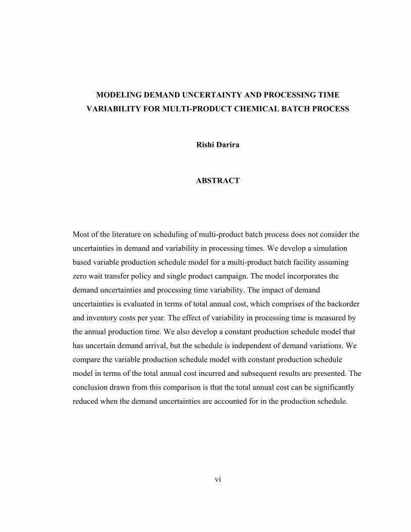
MODELING DEMAND UNCERTAINTY AND PROCESSING TIME
VARIABILITY FOR MULTI-PRODUCT CHEMICAL BATCH PROCESS
Rishi Darira
ABSTRACT
Most of the literature on scheduling of multi-product batch process does not consider the
uncertainties in demand and variability in processing times. We develop a simulation
based variable production schedule model for a multi-product batch facility assuming
zero wait transfer policy and single product campaign. The model incorporates the
demand uncertainties and processing time variability. The impact of demand
uncertainties is evaluated in terms of total annual cost, which comprises of the backorder
and inventory costs per year. The effect of variability in processing time is measured by
the annual production time. We also develop a constant production schedule model that
has uncertain demand arrival, but the schedule is independent of demand variations. We
compare the variable production schedule model with constant production schedule
model in terms of the total annual cost incurred and subsequent results are presented. The
conclusion drawn from this comparison is that the total annual cost can be significantly
reduced when the demand uncertainties are accounted for in the production schedule.
vi
CHAPTER 1
INTRODUCTION
Chemical processes are divided into two types continuous and batch. Chemicals are
manufactured in batches if production volumes are small. Batch processes are used in the
manufacture of pharmaceutical products, food, and certain types of chemicals. Batch
process is divided into multi-product plant or multi purpose plant. There are several
decisions involved in batch process. We would concentrate on the scheduling aspect
which can have a large economic impact. In most problems involving scheduling of batch
plants it is assumed that the problem data can be predetermined. We would explore
scheduling by incorporating uncertainties in data. The basic structure of the batch
process and scheduling concepts are explained in this chapter.
1.1 Multiple-Product Batch Plants
When a batch process is used to manufacture more than two products, two types of plants
arises, flowshop plants in which all products have the same recipe, and job shop plants
where the products do not require same recipe. Flow-shop plants are known as “multi-
product plants” and job shop plants are known as “multi-purpose plants.”
1.2 Types of Campaigns
The entire scheduling horizon is divided into planning periods in which cycles of
predetermined set of batches are produced. One option is to use single product campaigns
in which all batches of a given product which was predetermined to be produced in a
period are manufactured before switching to another product. The other option is to use
mixed product campaigns in which the batches are produced according to some selected
sequence. The inventory is lower when mixed product campaign is used but its efficiency
depends on the cleanup times between successive products. If the clean up times are
1
significantly large in comparison to the processing time then it is advisable to use single
product campaign to maximize production. Optimal sequence determination is also an
important aspect of batch process scheduling. An effective algorithm was proposed by
Birewar and Grossmann [1989] to determine optimal sequence.
1.3 Transfer Policies
The main types of transfer policies are explained below
1. Zero wait transfer
This transfer policy assumes that the batch at any stage would be transferred immediately
to the next stage. It is often used when intermediate storage vessel is not available due to
economic constraints or when storage is not allowed for the intermediate product. The
zero wait transfer because of its constraint of no wait is associated with higher cycle time
in comparison to other transfer policies. This policy has forces idle time between
successive batches and successive products [Rekalaitis et al, 1992].
2. No Intermediate Storage
This transfer policy allows holding the material inside the vessel until the next stage is
idle. Storage vessels are not required in this policy thus reducing the investment cost but
the production time increases due to holding.
3. Finite Intermediate Storage
This policy predetermines the approximate quantity of batches that require storage.
Optimal storage equipment can be purchase therefore reducing the investment cost.
4. Unlimited Intermediate Storage
This policy assumes that batches can be stored without any capacity limit in the storage
vessel. It is associated with lowest cycle time but requires large capital investment.
1.4 Uncertainties in Data
Most of the scheduling models that have been developed assume that all the data are
predetermined. Such models are said to be deterministic. In chemical plants there are
many factors such as equipment availability, processing times, demands of products and
costs causing uncertainty [Balasubramaniam and Grossmann, 2001]. These uncertainties
2
are common and can have undesirable costs attached. Thus these uncertainties should be
taken into account while scheduling.
1.5 Simulation as Modeling Tool
Mathematical programming involves making simplified assumptions. Simulation is a
process which mimics the process. It provides fast analysis of the schedule. Using
simulation for testing a schedule is economical. Simulation can be used for planning the
process, process development, process design and the manufacturing stage.
1.6 Thesis Organization
The organization of the thesis is as follows. Chapter 2 reviews the prior work in the area
of scheduling, scheduling with uncertainties in demand, processing time variation and
simulation of multi-product batch process. Chapter 3 describes the variable schedule
model which incorporates uncertainties in demand and processing time variability.
Various performance measures used to judge the effectiveness of the schedule are
explained. A constant schedule model is also described which would be compared to the
variable schedule model. Chapter 4 describes the modeling methodology used. It also
describes the formation of variable schedule model and constant schedule model for an
example problem. The results obtained are listed in Chapter 5. A statistical analysis of the
simulation runs is made leading to appropriate interpretations. Finally, Chapter 6
summarizes the entire thesis. It also includes the conclusions and areas of future research.
3
CHAPTER 2
LITERATURE REVIEW
Batch processing constitutes a significant fraction in the chemical process industries. For
example 80 percent of pharmaceutical and 65 percent of the food and beverage processes
are batch processes [Reeve, 1992]. Despite the development of design models and
techniques for batch processes, there is lack of comprehensive methodologies that can
properly address the many aspects involved in batch process [Reklaitis, 1990]. A
comprehensive overview on scheduling and planning of batch process was presented in
the book by Reklaitis et al [1992]
2.1 Process Design
A mixed integer non-linear programming problem was proposed by Graham et al [1979]
that minimized equipment cost. It also found optimal number of equipments and their
sizes. Zero wait policy was implemented. Branch and bound method could be used to
solve optimization problems, but it has limitations. Process merging was implemented by
Yeh and Reklaitis [1987] for single product plants. Birewar and Grossman [1989]
showed that process merging leads to lower investment cost. It was assumed that the
equipment sizes were continuous but practically equipment with standard discrete sizes is
available. Standard equipment sizes were considered by Voudouris and Grossmann
[1991]. Karimi and Reklaitis [1985] show that storage size effects cycle time and batch
size. The design of multi-product plants with intermediate storage was shown by Modi
and Karimi [1989]. Simulation can also be used to identify need of intermediate storage
and campaign. Birewar and Grossmann [1990] introduced scheduling at the design stage.
4
2.2 Scheduling Multi -Product Plant
Each product is produced in batches that determine the size factor of equipments thus
each batch is considered as a different entity for scheduling. All products follow the same
process stages. The unlimited intermediate storage, no intermediate storage, zero wait and
finite storage conditions are all treated as the options for transfer policies.
2.2.1 Unlimited Storage and Zero Wait Policies
Kuriyan and Reklaitis [1989] developed algorithms for the scheduling of multi product
batch plants with unlimited intermediate storage and zero wait policies. Minimizing make
span was their objective. A two-step method was used. The first step simplified
sequencing problem and the second step evaluated the sequence.
2.2.2 Finite Intermediate Storage
Many multi product batch plants operate under finite storage capacity policy. Kuriyan,
Joglekar and Reklaitis [1987] studied the use of finite intermediate storage in detail. They
used simulation to evaluate the production time. The study showed that simulation could
be effectively used for scheduling.
2.3 Single Product Campaign
Wellons and Reklaitis [1989] proposed a MINLP algorithm for determining the sequence
of a single product plant. The objective was to maximize the average production rate of
the plant.
2.4 Mixed Product Campaign
The output of a multi product plant can be increased by changing long single product
campaigns with combinations of batches of different products. The combinations are
repeated periodically. Mixed product campaigns studied by Birewar and Grossmann
[1989]. The set up times have an effect on the use of mixed product campaigns. The
inventory levels are lower when this policy is implemented.
5
2.5 Sequence Determination
Campaign lengths are determined by the demand size. The sequence of batches in the
campaign is an important factor to determine. Birewar and Grossmann [1989] proposed a
simple algorithm to determine optimal sequence. The objective was determination of
minimum cycle time. Inventory costs and process dictated by due dates has also been
studied. Sahinidis and Grossmann [1991] evaluated the problem of a multi-product
scheduling for constant demands. They developed an algorithm with cost minimization as
an objective.
2.6 Uncertainties in Demand
Petkov and Maranas [1998] proposed a method for designing a multi product batch plant
operating uncertain single product campaign. Demand follows Normal distribution. A
deterministic mixed-integer nonlinear programming problem was developed. Ierapetritou
and Pistikopoulos [1995] discussed the problem of designing multi product batch plants
with uncertain demands. They developed a non-linear optimization model with the
objective function including investment cost, net sales and penalty for unsatisfied
demand.
2.7 Variability in Processing Times
Pistikopoulos et al [1996] proposed a two-stage stochastic programming formulation. The
objective function included processing costs, sales and a penalty term accounting for not
meeting demand. Straub and Grossmann discussed the problem of evaluation and
optimization of probabilistic features in batch plants. They proposed computational
methods to determine size and number of equipment to maximize expected probabilistic
uncertainty. Constraint included the investment. Honkomp, Mockus and Reklaitis [1997]
compared three different models. The uniform time discretized model, non uniform
discretized model and model with scheduling uncertainty.
6
2.8 Markov Chain Approach to Unpaced Transfer Lines
Many researchers have studied unpaced transfer lines using Markov chain approach. A
parallel can be drawn between a transfer line and a chemical manufacturing facility. A
transfer line is a serial production system with multiple identical stages with same
processing time distribution. Initial studies concentrated on transfer lines with variability
in processing times with no buffers (zero-wait) and no breakdowns. Due to the process
time variability workstations are starved until the upstream station finishes its operation.
Similarly workstations are blocked until the downstream station finishes and can pass on
its job. It was observed that the system throughput decreases with the increase in the
processing time variability (measured by coefficient of variation) and the number of
stages. The impact of increase in coefficient of variation was very significant while the
impact of number of stages levels off after 5 or 6 stages [Conway et al, 1988]. It has
been reported by the authors that other than few simple cases which could be solved
using analytical approach, simulation was invariably used to study such systems. There
were other studies which included buffers (non-zero wait) to increase the productivity.
The effect of breakdowns on transfer lines with constant processing time was also studied
[Askin and Standridge, 1993].
2.9 Use of Simulation in Batch Process
Rippin [1983] has reviewed the literature on optimal operation of batch process
equipments. He has provided his view of methods available for designing and operating a
batch plant. The benefits of simulation at various stages of the commercialization process
are categorized by Petrides, Koulouris and Lagonikos [2002]. Simulation can be
effectively used for planning the process, process development, process design and the
manufacturing stage.
2.10 Summary
The work done for the design and scheduling of a multi-product batch plant by
researchers was reviewed in this chapter. The design aspect involves allocation of tasks to
the resources and the use of intermediate storage if possible. The use of intermediate
7
storage decreases the cycle time but it increases the investment cost. Algorithms
optimizing the use of intermediate storage with objective to minimize the cost were
studied. The scheduling of a multi-product batch plant deals with the sequencing of
products. Birewar and Grossmann [1989] have developed effective algorithm that
determines optimal sequence of products while incorporating clean-up times and slack
times in the algorithm with minimizing the cycle time as the objective.
A lot of work in operations planning has been done to develop deterministic
models. The problem data is known in advance in deterministic models. There can be
uncertainty in real problems in factors like processing times and demands. The common
approach to deal with these uncertainties is with probabilistic model. Operations planning
considering uncertainties in various factors are an important aspect as this can have
considerable economic implications. This research incorporates uncertainties in
processing times and variable demands of products in a multi-product batch plant with
multiple stages. The next chapter describes the model features and performance
measures.
8
CHAPTER 3
MODELING FEATURES
The scheduling of a multi-product batch process was discussed in the previous chapters.
This chapter describes a variable schedule model based on multi-product batch process.
The model features and its performance measures are shown below.
3.1 Single Product Campaign Model with Zero Wait Policy
In a multi-product plant all products follow the same sequence of operation. The first step
is to decide a transfer policy suitable for the process. The different types of transfer
policies are described in chapter one. If we select policies like unlimited intermediate
storage policies or finite intermediate storage transfer policy then investments would
have to be made on storage vessels. The constraints on the investment cost lead us to
assume zero wait policy
The type of production campaign is decided next. The campaign type
selected is used for manufacturing a specified number of batches for the various products
in a planning period or cycle. One option is to use single product campaigns in which all
batches of a given product are manufactured before changing to another product. The
other option is to use mixed product campaigns in which batches are produced according
to a selected sequence during a production cycle. The inventory levels of individual
products in single product campaign are greater than the mixed product campaign. Thus
inventory-carrying costs are higher in single product campaigns. Efficiency of the mixed
product campaign depends on the cleanup times that are needed after successive
products. If clean up times are very small compared to the processing time, mixed-
product campaign would be preferred over single product campaign. In this research, we
assume that the clean up times are significantly large thus we select single product
campaign. The optimal sequence of products during a cycle for is determined with the
9
help of an algorithm and a graphical method proposed by Birewar and Grossmann
[1989]. Their algorithm for single product campaign is categorized below. It explains that
some idle time is forced in zero wait policy. In their algorithm, SLikj denotes the
minimum forced idle time between the batches of product i and k in stage j. These slack
times (forced idle time) between two products could be predetermined by calculation.
The processing time of process i in stage j was indicated by tij. The total number of
batches of product i produced is ni. The cycle time (CT) for unlimited intermediate
storage is given in Equation 3.1.
CT = max j=1... M (∑=
Np
i
n1
i tij) (3.1)
The slack time was accounted for by making the cyclic sequence consist of pairs
of batches of products. For each pair, NPRSik was defined as the number of times product
i is followed by product k (i, k = 1…Np) in the schedule. Equation 3.2 shows the
succeeding constraint and 3.3 shows the preceding constraint for sequencing. Equation
3.4 gives the cycle times of each stage. The equality sign in Equation 3.5 enforces single
product campaign.
Min CT
Subject to
∑=
Np
k 1NPRSik = ni i= 1… NP (3.2)
∑=
Np
i 1NPRSik = nk k=1… NP (3.3)
CT ≥ n∑=
Np
i 1i tij + ∑ NPRS
=
Np
i 1∑=
Np
k 1ik SL ikj j= 1… M (3.4)
NPRSii = ni – 1 i = 1… NP (3.5)
CT ≥ 0, NPRSik ≥ 0 i, k = 1… NP (3.6)
The solution of this algorithm provides the values of NPRSik for combinations of
products i and k. The optimal sequence could then be calculated by a simple graphical
method.
10
3.2 Modeling Uncertainties
This objective of this research is to study the impact of the two of the uncertain
conditions that a chemical processing facility faces: uncertain demand and variable
processing time. The following subsections outline how these have been modeled in this
thesis.
3.2.1 Uncertain Demand Arrival
The total scheduling horizon would be divided into equal periods, which are called as the
planning periods. The demand arriving at each period is assumed to be variable. The
Poisson distribution can model this variability. It is a discrete distribution which gives the
average number of events in the given time interval. The Poisson distribution is
determined by one parameter lambda, indicating the mean of the distribution.
The variability in demand can also be modeled by a continuous distribution.
Normal distribution can be used to model demand variability. It is largely accepted that
Normal distribution covers the important features of uncertain demands. Theoretical
reasoning in use of Normal distribution can be based on central limit theorem as the
demands are affected by a large number of probabilistic events. [Petkov and Maranas,
1998].
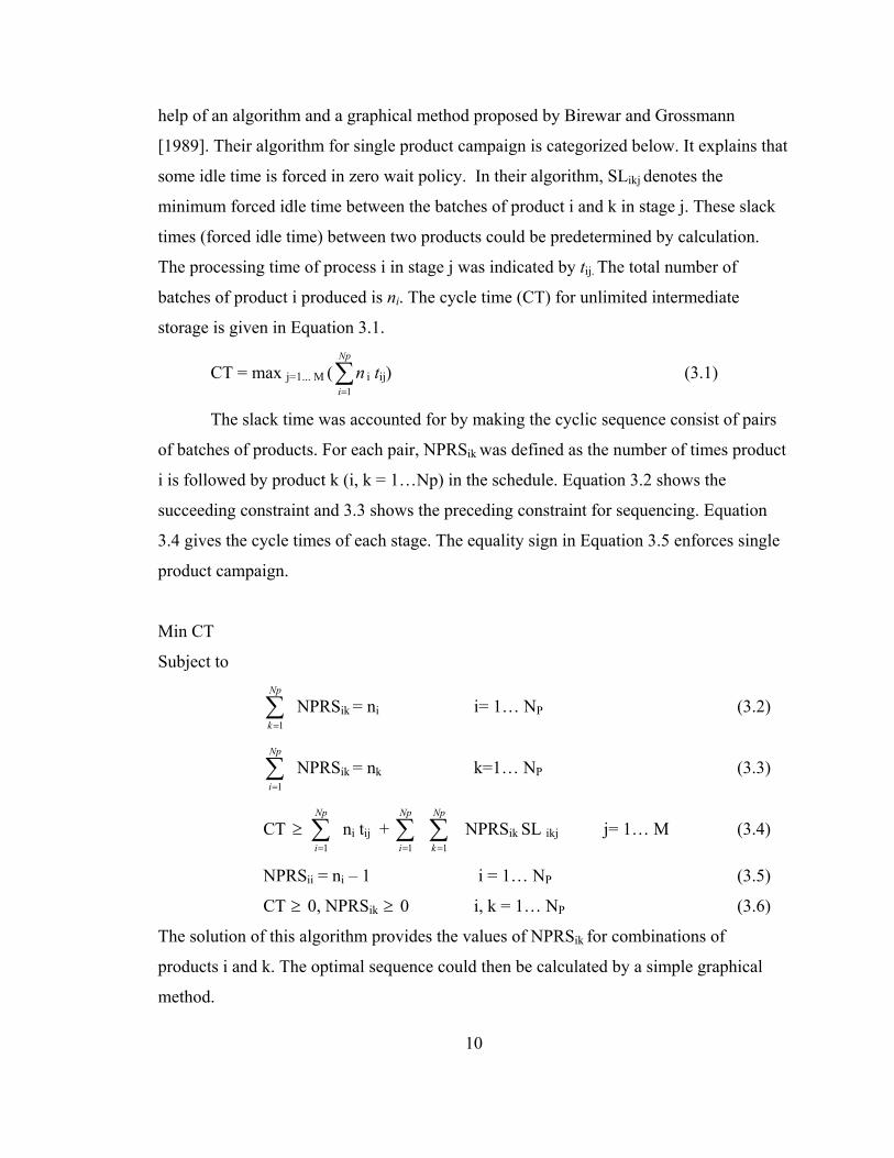
Uniform distribution can also be used to model demand arrival. The three
distributions would be compared in terms of their effect on the performance measure.
The three distributions used to model the demand variation in this thesis are given in
Table 3.1.
Table 3.1: Demand Distribution
Demand Distribution
Uniform
Normal
Poisson
11
3.2.2 Processing Time Variation
In chemical processes the processing times at each stage varies depending on factors such
as the efficiency of the equipment and quality of material being processed. This variation
is continuously distributed. The uncertainty in processing times would be modeled using
Normal distribution. The Normal is a two-parameter probability distribution described by
mean and standard deviation (µ and σ).
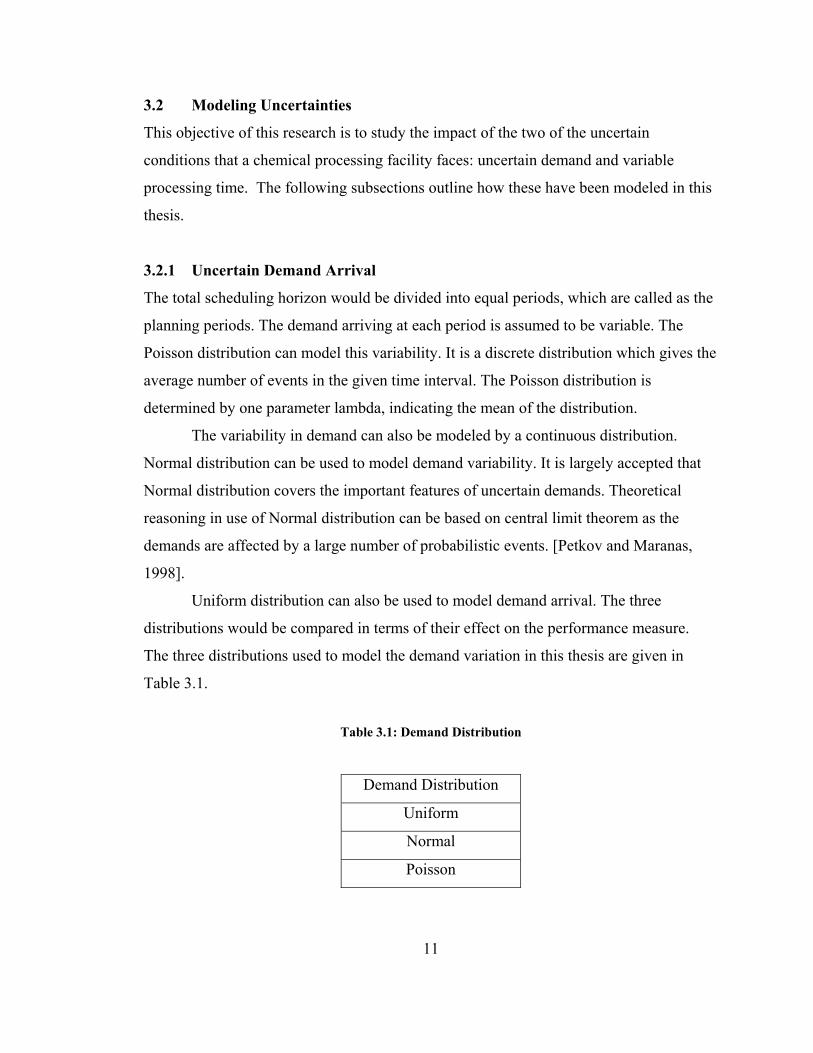
The uncertainty in processing times is assumed to be at two levels -- high and
low. The values of coefficient of variation corresponding to the level of uncertainty are
indicated in Table 3.1. For example when coefficient of variation is 0.05 (low level of
uncertainty) and the mean processing time is 7 hours then the standard deviation is 0.35
hours (from Equation 3.7), therefore 95 percent of the times the processing times will lie
between 6.3 hours and 7.7 hours (2 σ limit). When the coefficient of variation is 0.1 (high
level of uncertainty) with mean processing time as 7 hours the standard deviation is 0.7
hours thus 95 percent of time the processing time would lie within 5.6 hours and 8.4
hours. The effect of theses variations when they are at high level or low level would be
modeled and analyzed. The variability is shown in Table 3.2.
Table 3.2: Coefficients of Variation in Processing Times
Level of Uncertainty Coefficient of Variation
None 0.00
Low 0.05
High 0.10
3.3 Operating Policy
The batch size is assumed to be constant for each product. An optimal design of the
process with the objective of minimizing the cycle time is considered. The demand is
assumed to arrive at the beginning of the planning period. The demands have to be met
by the end of the planning period. The following two cases arise for this model.
12
3.3.1 Extra Capacity Utilization: Use of Inventory
If the demands were met before the end of planning period, the remaining time in that
period can be used to utilize the capacity. The product would then be stored as inventory.
Thus we have to determine which product should be produced and in what quantity. The
time remaining in a particular planning period is calculated. We determine the minimum
demand ratios of the products. For example consider four products have to be produced
and their mean periodic demand is 14, 7, 7 and 21 respectively. Thus their minimum
weekly demand ratio will be 2, 1, 1 and 3. The mean production time for this minimum
demand ratio is then calculated. This production time is then compared to the time
remaining in a period. If the time remaining is less than the production time of the
products in their minimum demand ratio then the product with the highest demand is
produced first. The remaining time is divided by the cycle time of the product with
highest demand. This would give the number of batches of that product that can be made.
We limit its production till its minimum demand ratio that is 3 units as in example
explained. The product with the second highest demand is produced next considering its
minimum demand ratio. Thus the production continues till the time remaining is not
sufficient to produce any more batches. The capacity would not be utilized for the
residual time remaining.
If the time remaining is greater than the production time of the products in their
minimum demand ratios then we check if the multiples of the minimum demand ratio can
be produced. Based on the above example it would be checked if 4, 2, 2 and 6 batches of
the products could be produced. If enough time is remaining for this then we produce it.
We produce in higher demand ratios because the clean up times are reduced. They are
produced till the time remaining is less than the production time of a particular ratio. The
lower ratio is then considered till there is not enough time remaining to produce the
minimum demand ratio The production then continues according to the scenario
described above when time remaining is less than the production time of the minimum
demand ratio cycle time.
13
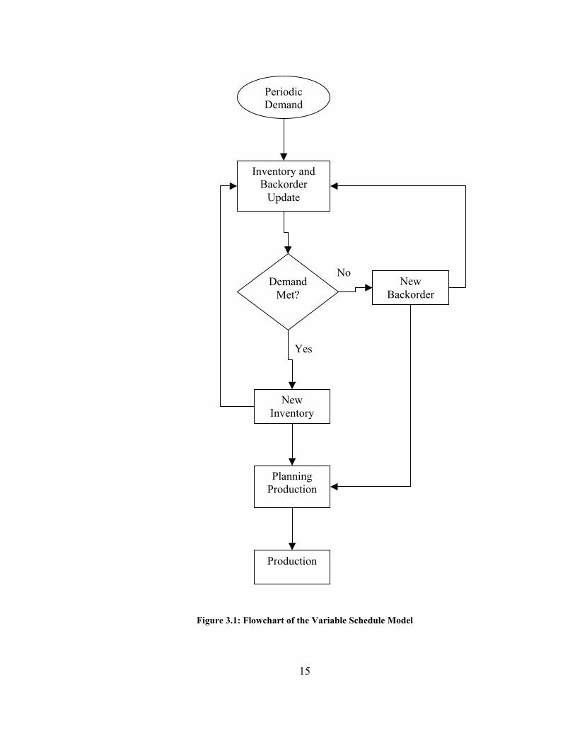
3.3.2 Backordering Due to Insufficient Capacity
If the demands are not satisfied in a particular planning period then the options are to
either consider lost sales or backorder the product so that it is produced in the next
period. Lost sales lead to loss of profit and goodwill among customers. The customers
also tend to wait for some more time since they have already waited for the time of
planning period. Thus the unsatisfied demand in a planning period in this model would be
considered backordered. The backordered products are added to their respective new
period demands and they are produced in the next cycle according to the sequence
minimizing the cycle time. Figure 3.1 shows the flowchart of the process.
3.3.3 Modeling Zero Wait Policy
We assume zero wait policy which results in forced idle times between batches of
products. We have to make sure that there is no waiting or queues of intermediate
products. This would be done by forced delay between successive batches and between
successive products. The forced delay between successive batches would be the cycle
time of that particular product. The delay between successive products would include the
cycle time and the clean up times. For the case with variable processing times zero wait
policy would be implemented by holding the batch in a stage until the next stage is idle.
3.4 Constant Production Model
Most of the literature for scheduling of a multi-product batch plant does not incorporate
uncertainties in demand. A constant production model would also be developed in this
thesis. This model would have uncertainties in demand but the schedule would be fixed.
If excess demand arrives in a planning period then the extra batches are backordered and
if insufficient demand arrives then inventory will be allowed to build.
14
Periodic Demand
Inventory and Backorder
Update
No New
Backorder Demand
Met?
Yes
New Inventory
Planning Production
Production
Figure 3.1: Flowchart of the Variable Schedule Model
15
3.5 Summary
This chapter outlined the model features. The modeling problem includes a multi –
product batch plant. Zero wait policy is assumed due to investment constraints, because
for other transfer policies investment has to be made on storage vessels. Single product
campaign is implemented to minimize to production time. The operating optimal
sequence is obtained from the algorithm proposed by Birewar and Grossmann [1989].
Uncertainties in demand arrival and processing time variability would be modeled.
Various distributions for demand arrival and their effects on the performance measures
would be analyzed. A constant production model would be developed which would be
compared to the variable schedule model. The next chapter explains the model
development and the performance measures used.
16
CHAPTER 4
MODEL DEVELOPMENT
A multi-product batch facility with multiple stages is modeled. Zero wait transfer policy
is assumed. The entire scheduling cycle is divided into equal planning periods. Single
product campaign is assumed within a cycle. The processing times and the demands of
products are assumed to be variable. If demands are not met in a planning period the
product is backordered. If the demand is met before the end of planning period then the
excess capacity is utilized to make products for inventory to be used in the next cycle. A
simulation model using ARENA simulation software is developed. The model is then
used as a vehicle to determine the impact of the demand uncertainties on the backorders
and inventory accumulation and the processing time variability on production cycle time.
Finally, the performance of the variable schedule model will be compared with the
constant schedule model.
4.1 Modeling Method
Simulation was used to model the process. Simulation mimics the behavior of real
systems, usually on a computer with appropriate software. Simulation has become very
popular with the evolution of computers and software. The purpose of simulation is to
mimic the uncertainties in demand arrival and the processing times. The effect of these
uncertainties is evaluated.
4.2 ARENA as Simulation Software
Arena is simulation software which has flexible model building capabilities. It has
excellent features for statistics collection. The model with uncertainties in demand and
processing times in a multistage batch process with zero wait policy is created by using
the Basic process, advanced process, advanced transfer and blocks templates.
17
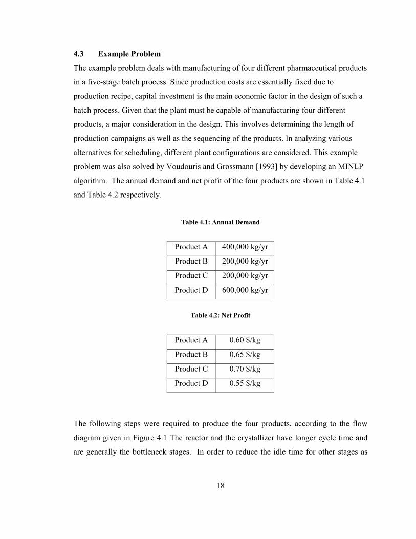
4.3 Example Problem
The example problem deals with manufacturing of four different pharmaceutical products
in a five-stage batch process. Since production costs are essentially fixed due to
production recipe, capital investment is the main economic factor in the design of such a
batch process. Given that the plant must be capable of manufacturing four different
products, a major consideration in the design. This involves determining the length of
production campaigns as well as the sequencing of the products. In analyzing various
alternatives for scheduling, different plant configurations are considered. This example
problem was also solved by Voudouris and Grossmann [1993] by developing an MINLP
algorithm. The annual demand and net profit of the four products are shown in Table 4.1
and Table 4.2 respectively.
Table 4.1: Annual Demand
Product A 400,000 kg/yr
Product B 200,000 kg/yr
Product C 200,000 kg/yr
Product D 600,000 kg/yr
Table 4.2: Net Profit
Product A 0.60 $/kg
Product B 0.65 $/kg
Product C 0.70 $/kg
Product D 0.55 $/kg
The following steps were required to produce the four products, according to the flow
diagram given in Figure 4.1 The reactor and the crystallizer have longer cycle time and
are generally the bottleneck stages. In order to reduce the idle time for other stages as
18
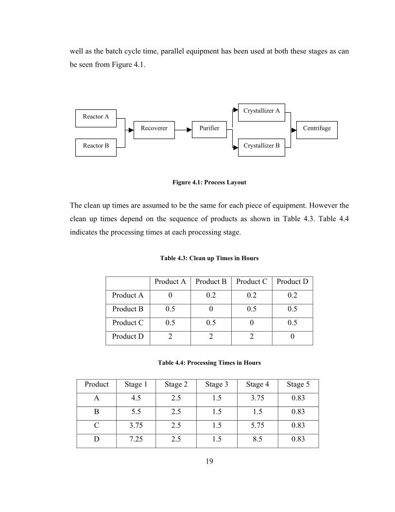
well as the batch cycle time, parallel equipment has been used at both these stages as can
be seen from Figure 4.1.
Recoverer Purifier
Crystallizer A
Crystallizer B
Reactor A
Centrifuge
Reactor B
Figure 4.1: Process Layout
The clean up times are assumed to be the same for each piece of equipment. However the
clean up times depend on the sequence of products as shown in Table 4.3. Table 4.4
indicates the processing times at each processing stage.
Table 4.3: Clean up Times in Hours
Product A Product B Product C Product D
Product A 0 0.2 0.2 0.2
Product B 0.5 0 0.5 0.5
Product C 0.5 0.5 0 0.5
Product D 2 2 2 0
Table 4.4: Processing Times in Hours
Product Stage 1 Stage 2 Stage 3 Stage 4 Stage 5
A 4.5 2.5 1.5 3.75 0.83
B 5.5 2.5 1.5 1.5 0.83
C 3.75 2.5 1.5 5.75 0.83
D 7.25 2.5 1.5 8.5 0.83
19
4.4 Assumptions
1. The time to transfer products between units and the time to fill and empty vessels is
negligible.
2. Demand arrives in batches. The batch size for all the products is the same. The batch
size is assumed to be 600 kilograms based on economic design considerations.
3. Backorder cost is two times the cost of inventory.
4. The demand is assumed to arrive at the beginning of the period and is satisfied at the
end of the planning period
5. The process design is optimal.
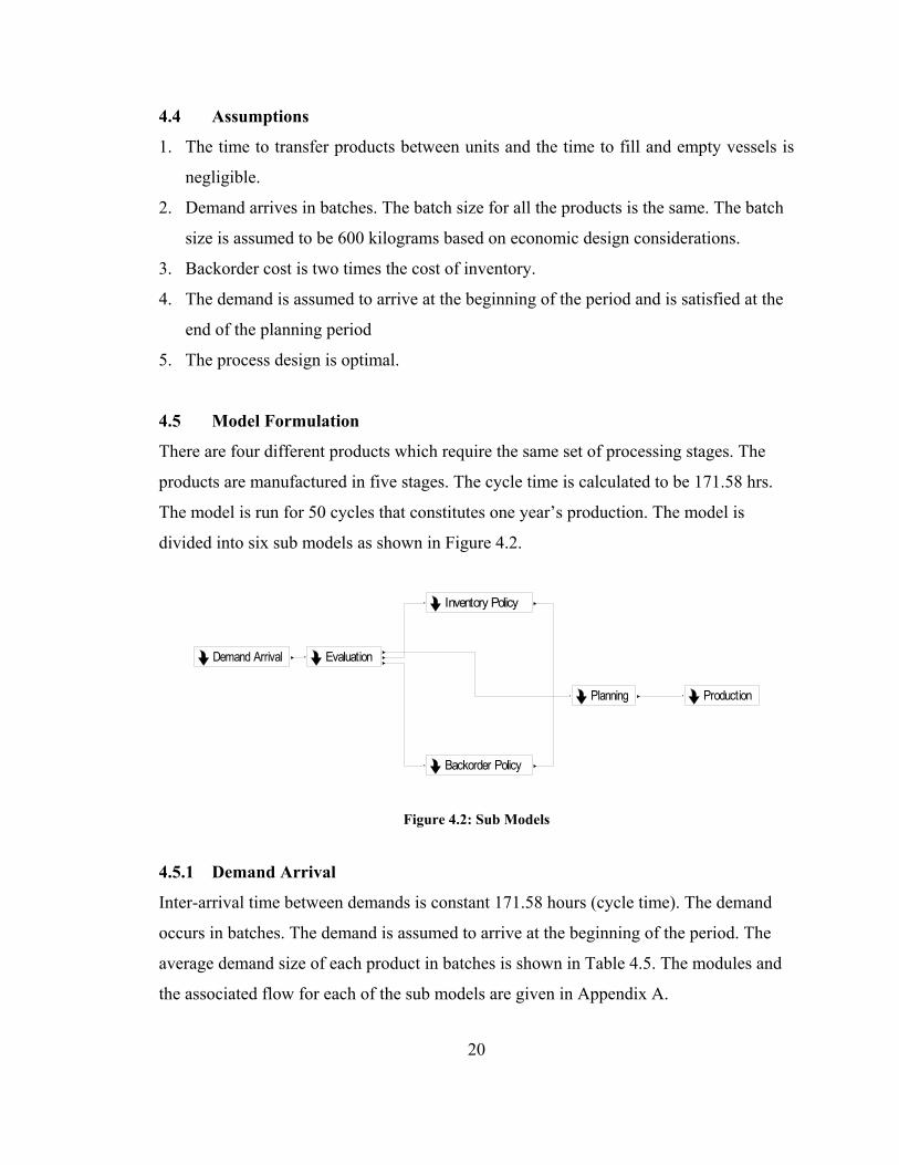
4.5 Model Formulation
There are four different products which require the same set of processing stages. The
products are manufactured in five stages. The cycle time is calculated to be 171.58 hrs.
The model is run for 50 cycles that constitutes one year’s production. The model is
divided into six sub models as shown in Figure 4.2.
Evaluation
Production
Demand Arrival
Inventory Policy
Backorder Policy
Planning
Figure 4.2: Sub Models
4.5.1 Demand Arrival
Inter-arrival time between demands is constant 171.58 hours (cycle time). The demand
occurs in batches. The demand is assumed to arrive at the beginning of the period. The
average demand size of each product in batches is shown in Table 4.5. The modules and
the associated flow for each of the sub models are given in Appendix A.
20
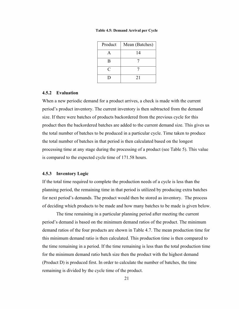
Table 4.5: Demand Arrival per Cycle
Product Mean (Batches)
A 14
B 7
C 7
D 21
4.5.2 Evaluation
When a new periodic demand for a product arrives, a check is made with the current
period’s product inventory. The current inventory is then subtracted from the demand
size. If there were batches of products backordered from the previous cycle for this
product then the backordered batches are added to the current demand size. This gives us
the total number of batches to be produced in a particular cycle. Time taken to produce
the total number of batches in that period is then calculated based on the longest
processing time at any stage during the processing of a product (see Table 5). This value
is compared to the expected cycle time of 171.58 hours.
4.5.3 Inventory Logic
If the total time required to complete the production needs of a cycle is less than the
planning period, the remaining time in that period is utilized by producing extra batches
for next period’s demands. The product would then be stored as inventory. The process
of deciding which products to be made and how many batches to be made is given below.
The time remaining in a particular planning period after meeting the current
period’s demand is based on the minimum demand ratios of the product. The minimum
demand ratios of the four products are shown in Table 4.7. The mean production time for
this minimum demand ratio is then calculated. This production time is then compared to
the time remaining in a period. If the time remaining is less than the total production time
for the minimum demand ratio batch size then the product with the highest demand
(Product D) is produced first. In order to calculate the number of batches, the time
remaining is divided by the cycle time of the product.
21
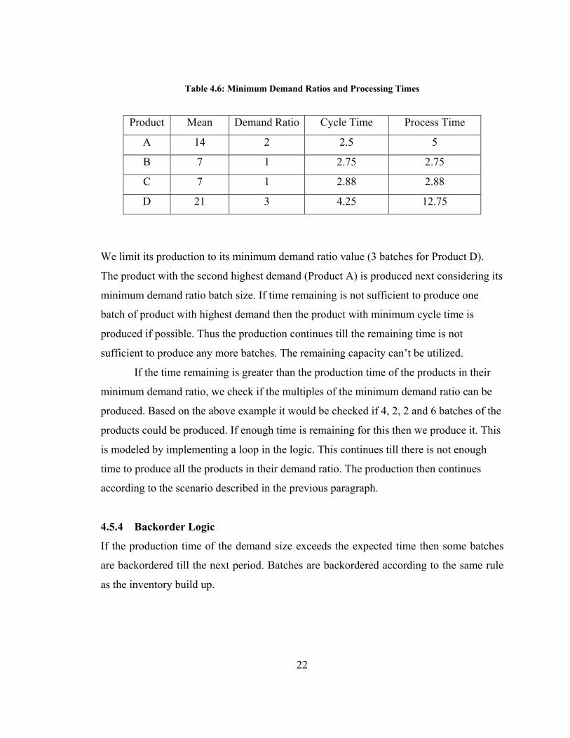
Table 4.6: Minimum Demand Ratios and Processing Times
Product Mean Demand Ratio Cycle Time Process Time
A 14 2 2.5 5
B 7 1 2.75 2.75
C 7 1 2.88 2.88
D 21 3 4.25 12.75
We limit its production to its minimum demand ratio value (3 batches for Product D).
The product with the second highest demand (Product A) is produced next considering its
minimum demand ratio batch size. If time remaining is not sufficient to produce one
batch of product with highest demand then the product with minimum cycle time is
produced if possible. Thus the production continues till the remaining time is not
sufficient to produce any more batches. The remaining capacity can’t be utilized.
If the time remaining is greater than the production time of the products in their
minimum demand ratio, we check if the multiples of the minimum demand ratio can be
produced. Based on the above example it would be checked if 4, 2, 2 and 6 batches of the
products could be produced. If enough time is remaining for this then we produce it. This
is modeled by implementing a loop in the logic. This continues till there is not enough
time to produce all the products in their demand ratio. The production then continues
according to the scenario described in the previous paragraph.
4.5.4 Backorder Logic
If the production time of the demand size exceeds the expected time then some batches
are backordered till the next period. Batches are backordered according to the same rule
as the inventory build up.
22
4.5.5 Planning
In this sub model the number of batches of each product is assigned a number. The first
batch of the first product is sent for production. A forced delay is implemented on
subsequent batches. The time of forced delay is the cycle time of that product. This
forced delay is implemented so that there is no waiting at the stages following the Zero
wait policy. After the last batch of the first product is released for production, the next
product’s first batch is signaled after a delay of the slack time. The slack time is
calculated by constructing Gantt charts. This prevents waiting in stages. The slack time
includes the cycle time of the product and the clean up times between successive
products. Due to variability in processing times if the production does not end in a
planning period the next cycle is not released. When the last batch of the last product is
released for production, it signals the next cycle’s release.
4.5.6 Production
The production sub-model consists of the five process stages. Zero wait policy is
modeled in the planning stage, but due to uncertainties in processing time there is bound
to be some waiting. Thus, this is modeled by incorporating hold and signal modules. A
batch is not released if the next stage is busy. As soon as the next stage is idle, this sends
a signal to the previous stage for the batches release. Thus, there is no waiting at the
resources.
4.6 Performance Measures
The performance of the process would be measured in terms of
1. Total Cost: This is the total cost of carrying inventory and backorder per year.
Backorder cost is assumed to be twice that of inventory cost.
2. Annual Production Time: This is the time taken to satisfy the demand for 50
cycles.
23
4.7 Model with Fixed Production Schedule
Most of the literature for scheduling of multi-product batch plant does not include
demand uncertainties. It would be interesting to see if the constant production schedule
misinterprets the annual inventory and backorder generated due to demand uncertainties.
Thus a simulation model was developed for the same example problem where the
production schedule is fixed. The constant production schedule model has uncertain
demand arrival, but the schedule is independent of demand variations. Total cost for
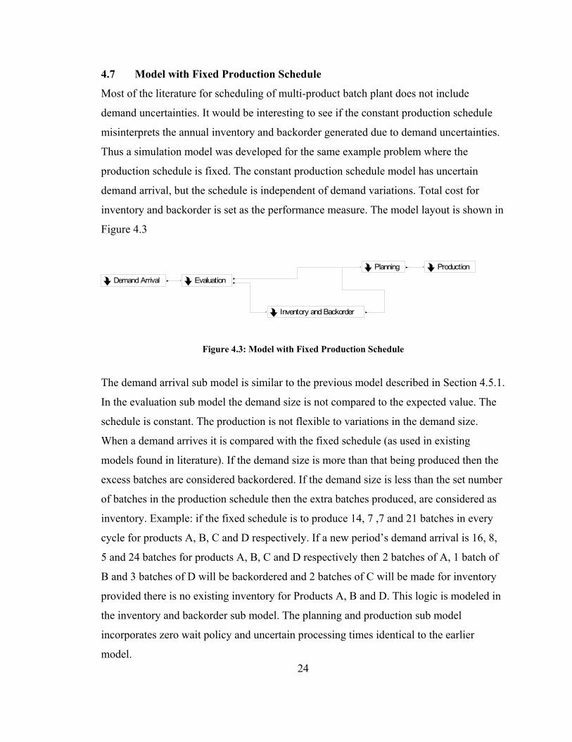
inventory and backorder is set as the performance measure. The model layout is shown in
Figure 4.3
Evaluation
Production
Demand Arrival
Inventory and Backorder
Planning
Figure 4.3: Model with Fixed Production Schedule
24
The demand arrival sub model is similar to the previous model described in Section 4.5.1.
In the evaluation sub model the demand size is not compared to the expected value. The
schedule is constant. The production is not flexible to variations in the demand size.
When a demand arrives it is compared with the fixed schedule (as used in existing
models found in literature). If the demand size is more than that being produced then the
excess batches are considered backordered. If the demand size is less than the set number
of batches in the production schedule then the extra batches produced, are considered as
inventory. Example: if the fixed schedule is to produce 14, 7 ,7 and 21 batches in every
cycle for products A, B, C and D respectively. If a new period’s demand arrival is 16, 8,
5 and 24 batches for products A, B, C and D respectively then 2 batches of A, 1 batch of
B and 3 batches of D will be backordered and 2 batches of C will be made for inventory
provided there is no existing inventory for Products A, B and D. This logic is modeled in
the inventory and backorder sub model. The planning and production sub model
incorporates zero wait policy and uncertain processing times identical to the earlier
model.
4.8 Summary
In this chapter, an Arena based simulation model was developed to mimic the process of
multi-product batch production with zero wait policy and single product campaign. This
model had a variable production schedule which incorporated demand uncertainties and
variation in processing time. The model features, formulation, assumptions and
performance measures were discussed. A constant schedule model with uncertainties in
demand was also developed to see if it misinterprets the annual inventory and backorder
generated due to demand uncertainties. The next chapter shows the results and analysis.
25
CHAPTER 5
RESULTS AND ANALYSIS
The previous chapter explained the model formulation and the performance measures of
the process. The model was run and the results obtained are presented in this chapter.
Variability in demand and processing times are analyzed for the variable schedule model.
Sensitivity analysis is performed for the backorder to inventory cost ratio and the quantity
of backorder and inventory. Demand distributions with higher uncertainty are also
analyzed. Finally a two factorial design is presented to see the effect of the variable
demand on the variable production schedule and the constant production schedule.
Coefficient of variation (CV) will be used as a measure of uncertainty or
variability associated with the demand and processing times in this thesis. The CV is a
better measure of variability since it takes into account the mean value as well. The CV
is defined as
C.V = µσ / (5.1)
Where, σ is the standard deviation and µ is the mean.
5.1 Uncertain Demand
The mean demand for the four products is given earlier in Table 4.6. For products A, B,
C and D these values are 14, 7, 7, and 21 batches respectively. The effect of demand
uncertainty is analyzed for different distributions shown below.
1. Normal Distribution
The standard deviation assumed for the periodic demand is shown in Table 5.1 which
results into a coefficient of variation of approximately 0.14.
26
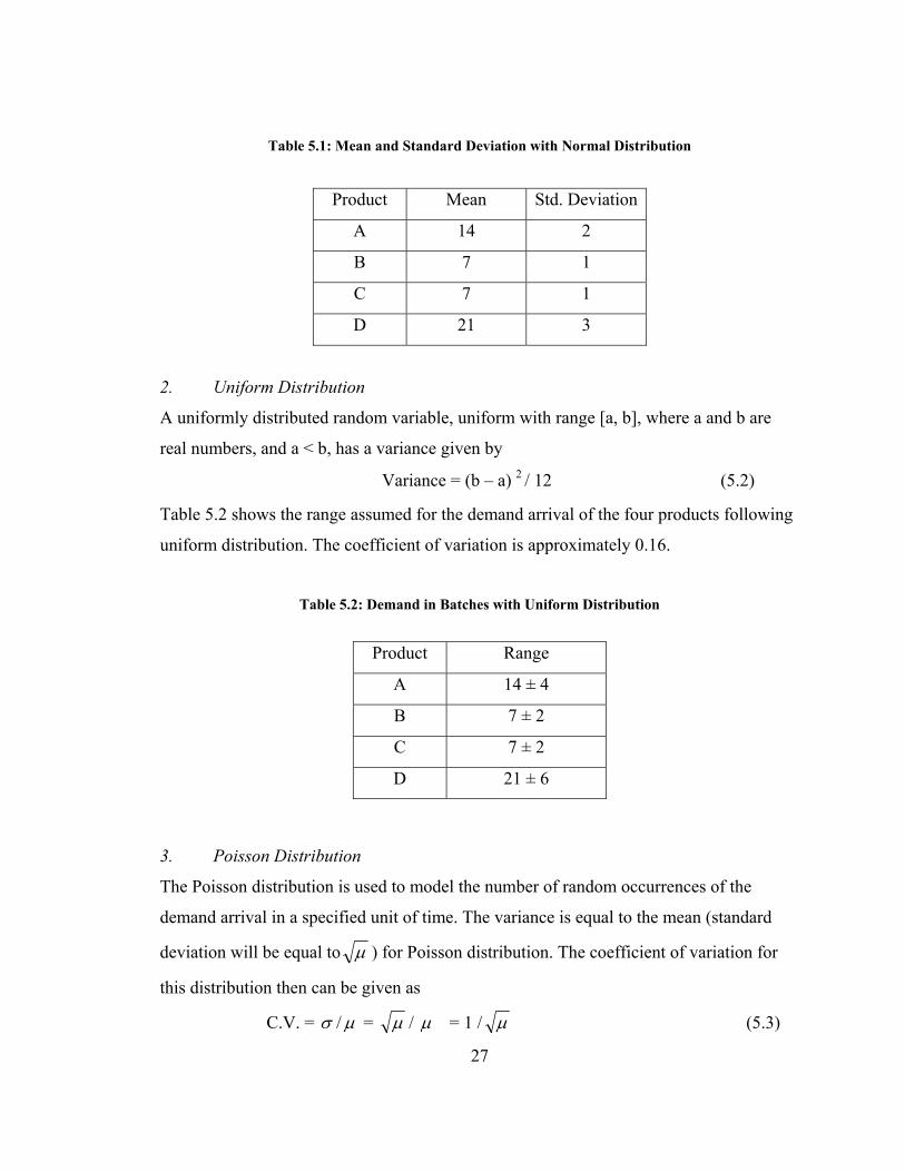
Table 5.1: Mean and Standard Deviation with Normal Distribution
Product Mean Std. Deviation
A 14 2
B 7 1
C 7 1
D 21 3
2. Uniform Distribution
A uniformly distributed random variable, uniform with range [a, b], where a and b are
real numbers, and a < b, has a variance given by
Variance = (b – a) 2 / 12 (5.2)
Table 5.2 shows the range assumed for the demand arrival of the four products following
uniform distribution. The coefficient of variation is approximately 0.16.
Table 5.2: Demand in Batches with Uniform Distribution
Product Range
A 14 ± 4
B 7 ± 2
C 7 ± 2
D 21 ± 6
3. Poisson Distribution
The Poisson distribution is used to model the number of random occurrences of the
demand arrival in a specified unit of time. The variance is equal to the mean (standard
deviation will be equal to µ ) for Poisson distribution. The coefficient of variation for
this distribution then can be given as
C.V. = µσ / = µ / µ = 1 / µ (5.3)
27
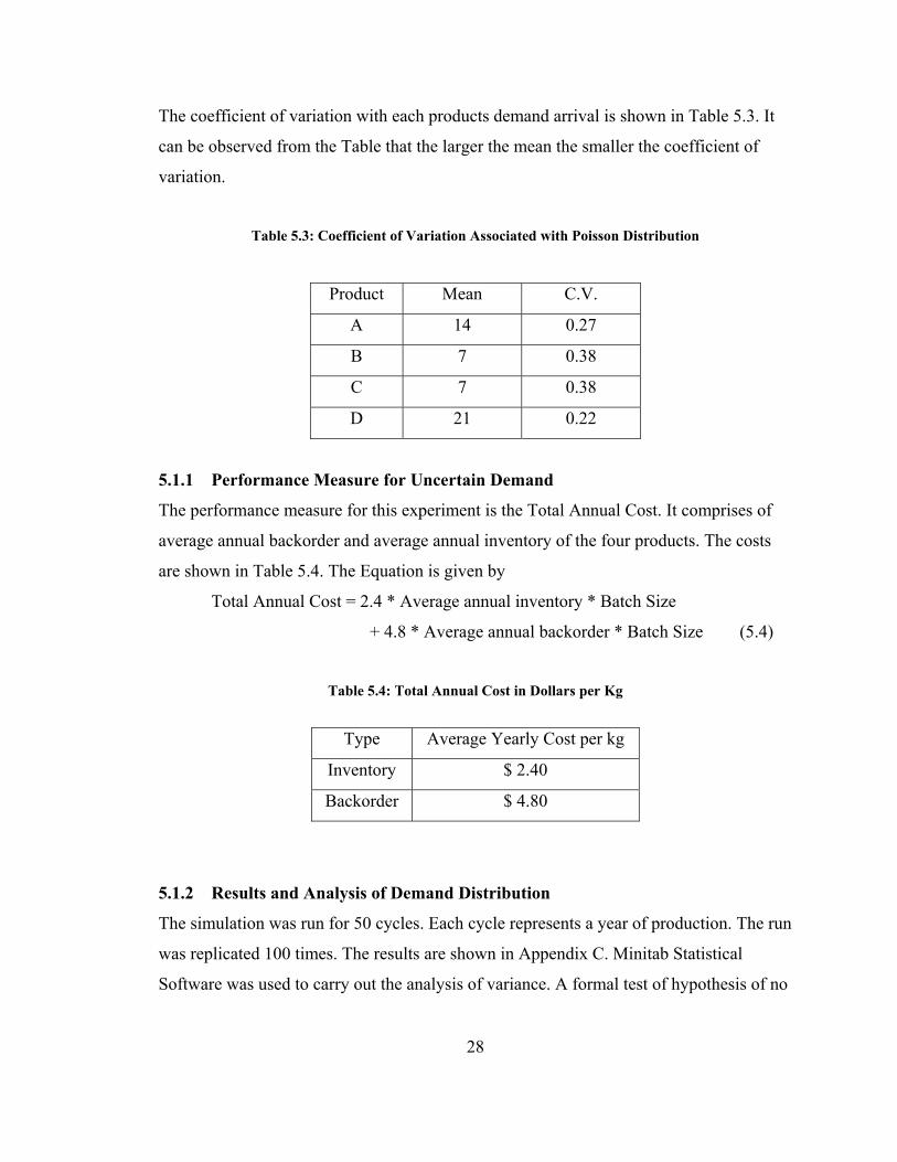
The coefficient of variation with each products demand arrival is shown in Table 5.3. It
can be observed from the Table that the larger the mean the smaller the coefficient of
variation.
Table 5.3: Coefficient of Variation Associated with Poisson Distribution
Product Mean C.V.
A 14 0.27
B 7 0.38
C 7 0.38
D 21 0.22
5.1.1 Performance Measure for Uncertain Demand
The performance measure for this experiment is the Total Annual Cost. It comprises of
average annual backorder and average annual inventory of the four products. The costs
are shown in Table 5.4. The Equation is given by
Total Annual Cost = 2.4 * Average annual inventory * Batch Size
+ 4.8 * Average annual backorder * Batch Size (5.4)
Table 5.4: Total Annual Cost in Dollars per Kg
Type Average Yearly Cost per kg
Inventory $ 2.40
Backorder $ 4.80
5.1.2 Results and Analysis of Demand Distribution
The simulation was run for 50 cycles. Each cycle represents a year of production. The run
was replicated 100 times. The results are shown in Appendix C. Minitab Statistical
Software was used to carry out the analysis of variance. A formal test of hypothesis of no
28
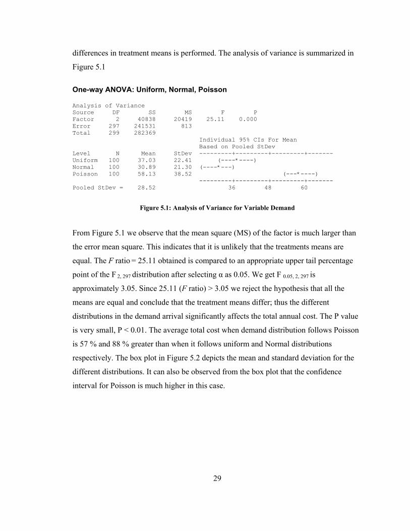
differences in treatment means is performed. The analysis of variance is summarized in
Figure 5.1
One-way ANOVA: Uniform, Normal, Poisson Analysis of Variance Source DF SS MS F P Factor 2 40838 20419 25.11 0.000 Error 297 241531 813 Total 299 282369 Individual 95% CIs For Mean Based on Pooled StDev Level N Mean StDev ---------+---------+---------+------- Uniform 100 37.03 22.41 (----*----) Normal 100 30.89 21.30 (----*---) Poisson 100 58.13 38.52 (---*----) ---------+---------+---------+------- Pooled StDev = 28.52 36 48 60
Figure 5.1: Analysis of Variance for Variable Demand
From Figure 5.1 we observe that the mean square (MS) of the factor is much larger than
the error mean square. This indicates that it is unlikely that the treatments means are
equal. The F ratio = 25.11 obtained is compared to an appropriate upper tail percentage
point of the F 2, 297 distribution after selecting α as 0.05. We get F 0.05, 2, 297 is
approximately 3.05. Since 25.11 (F ratio) > 3.05 we reject the hypothesis that all the
means are equal and conclude that the treatment means differ; thus the different
distributions in the demand arrival significantly affects the total annual cost. The P value
is very small, P < 0.01. The average total cost when demand distribution follows Poisson
is 57 % and 88 % greater than when it follows uniform and Normal distributions
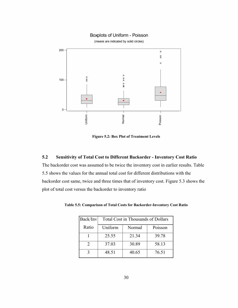
respectively. The box plot in Figure 5.2 depicts the mean and standard deviation for the
different distributions. It can also be observed from the box plot that the confidence
interval for Poisson is much higher in this case.
29
Pois
son
Nor
mal
Uni
form
200
100
0
Boxplots of Uniform - Poisson(means are indicated by solid circles)
Figure 5.2: Box Plot of Treatment Levels
5.2 Sensitivity of Total Cost to Different Backorder - Inventory Cost Ratio
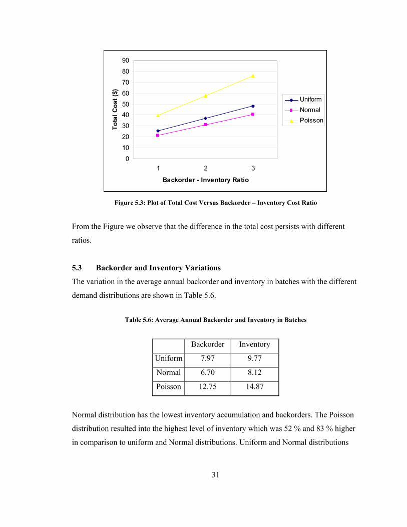
The backorder cost was assumed to be twice the inventory cost in earlier results. Table
5.5 shows the values for the annual total cost for different distributions with the
backorder cost same, twice and three times that of inventory cost. Figure 5.3 shows the
plot of total cost versus the backorder to inventory ratio
Table 5.5: Comparison of Total Costs for Backorder-Inventory Cost Ratio
Total Cost in Thousands of Dollars Back/Inv
Ratio Uniform Normal Poisson
1 25.55 21.34 39.78
2 37.03 30.89 58.13
3 48.51 40.65 76.51
30
0102030405060708090
1 2 3
Backorder - Inventory Ratio
Tota
l Cos
t ($)
UniformNormalPoisson
Figure 5.3: Plot of Total Cost Versus Backorder – Inventory Cost Ratio
From the Figure we observe that the difference in the total cost persists with different
ratios.
5.3 Backorder and Inventory Variations
The variation in the average annual backorder and inventory in batches with the different
demand distributions are shown in Table 5.6.
Table 5.6: Average Annual Backorder and Inventory in Batches
Backorder Inventory
Uniform 7.97 9.77
Normal 6.70 8.12
Poisson 12.75 14.87
Normal distribution has the lowest inventory accumulation and backorders. The Poisson
distribution resulted into the highest level of inventory which was 52 % and 83 % higher
in comparison to uniform and Normal distributions. Uniform and Normal distributions
31
have the same amount of backorder. The backorder is about 60 % higher in Poisson
distribution when compared to other distributions. Poisson distribution in this case has
the highest inventory accumulation and the largest amount of backorder thus resulting in
higher total annual cost.
5.4 Higher Variation for Normal and Uniform Distribution
It must be pointed that in the previous experiment to assess the impact of different
distributions, Normal and uniform distributions had much lower variability (CV of 0.14
and 0.16 with Normal and uniform respectively) compared to Poisson distribution
(average CV of 0.31). Poisson distribution had the highest total annual cost.
In order to see if the shape of the distribution or the variability has a greater
impact on the total annual cost, we ran the simulation model with larger variations in
Normal and uniform distributions. The standard deviation for Normal distribution is
shown in Table 5.7, the coefficient of variation is approximately 0.28. The range of
uniform distribution is increased to the values shown in Table 5.8. The coefficient of
variation for uniform distribution in this case is approximately 0.33. These values of CV
for Normal and uniform are now comparable to Poisson distribution.
Table 5.7: Mean and Standard Deviation for Normal Distribution
Product Mean Std. Deviation
A 14 4
B 7 2
C 7 2
D 21 6
32
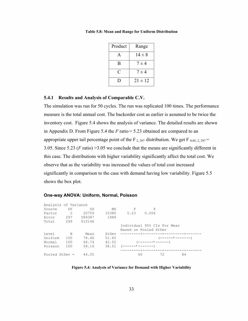
Table 5.8: Mean and Range for Uniform Distribution
Product Range
A 14 ± 8
B 7 ± 4
C 7 ± 4
D 21 ± 12
5.4.1 Results and Analysis of Comparable C.V.
The simulation was run for 50 cycles. The run was replicated 100 times. The performance
measure is the total annual cost. The backorder cost as earlier is assumed to be twice the
inventory cost. Figure 5.4 shows the analysis of variance. The detailed results are shown
in Appendix D. From Figure 5.4 the F ratio = 5.23 obtained are compared to an
appropriate upper tail percentage point of the F 2, 297 distribution. We get F 0.05, 2, 297 =
3.05. Since 5.23 (F ratio) >3.05 we conclude that the means are significantly different in
this case. The distributions with higher variability significantly affect the total cost. We
observe that as the variability was increased the values of total cost increased
significantly in comparison to the case with demand having low variability. Figure 5.5
shows the box plot.
One-way ANOVA: Uniform, Normal, Poisson Analysis of Variance Source DF SS MS F P Factor 2 20759 10380 5.23 0.006 Error 297 589387 1984 Total 299 610146 Individual 95% CIs For Mean Based on Pooled StDev Level N Mean StDev ---------+---------+---------+------- Uniform 100 78.46 51.60 (------*-------) Normal 100 66.74 42.52 (-------*------) Poisson 100 58.16 38.51 (------*-------) ---------+---------+---------+------- Pooled StDev = 44.55 60 72 84
Figure 5.4: Analysis of Variance for Demand with Higher Variability
33
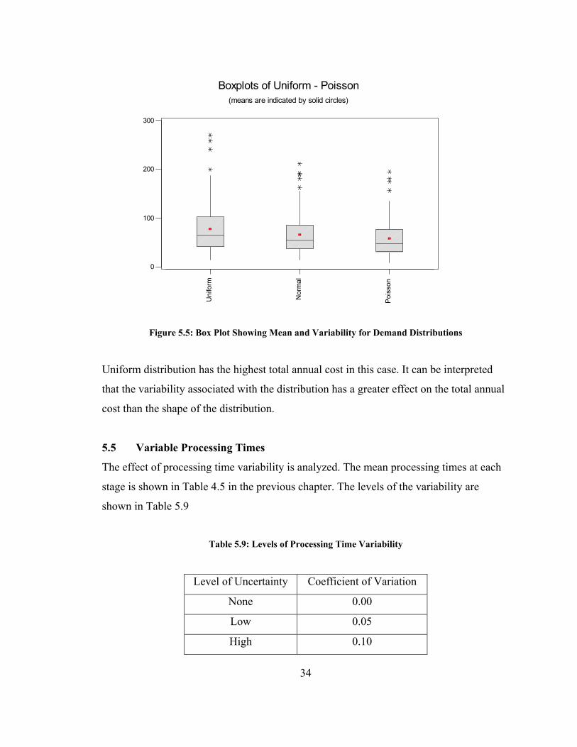
Pois
son
Nor
mal
Uni
form
300
200
100
0
Boxplots of Uniform - Poisson(means are indicated by solid circles)
Figure 5.5: Box Plot Showing Mean and Variability for Demand Distributions
Uniform distribution has the highest total annual cost in this case. It can be interpreted
that the variability associated with the distribution has a greater effect on the total annual
cost than the shape of the distribution.
5.5 Variable Processing Times
The effect of processing time variability is analyzed. The mean processing times at each
stage is shown in Table 4.5 in the previous chapter. The levels of the variability are
shown in Table 5.9
Table 5.9: Levels of Processing Time Variability
Level of Uncertainty Coefficient of Variation
None 0.00
Low 0.05
High 0.10
34
5.5.1 Performance Measure for Variable Processing Times
The performance measure is the time taken to complete 50 cycles (Annual Production
Time).
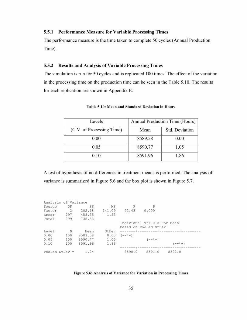
5.5.2 Results and Analysis of Variable Processing Times
The simulation is run for 50 cycles and is replicated 100 times. The effect of the variation
in the processing time on the production time can be seen in the Table 5.10. The results
for each replication are shown in Appendix E.
Table 5.10: Mean and Standard Deviation in Hours
Annual Production Time (Hours) Levels
(C.V. of Processing Time) Mean Std. Deviation
0.00 8589.58 0.00
0.05 8590.77 1.05
0.10 8591.96 1.86
A test of hypothesis of no differences in treatment means is performed. The analysis of
variance is summarized in Figure 5.6 and the box plot is shown in Figure 5.7.
Analysis of Variance Source DF SS MS F P Factor 2 282.18 141.09 92.43 0.000 Error 297 453.35 1.53 Total 299 735.53 Individual 95% CIs For Mean Based on Pooled StDev Level N Mean StDev -------+---------+---------+--------- 0.00 100 8589.58 0.00 (--*-) 0.05 100 8590.77 1.05 (--*-) 0.10 100 8591.96 1.86 (--*-) -------+---------+---------+--------- Pooled StDev = 1.24 8590.0 8591.0 8592.0
Figure 5.6: Analysis of Variance for Variation in Processing Times
35
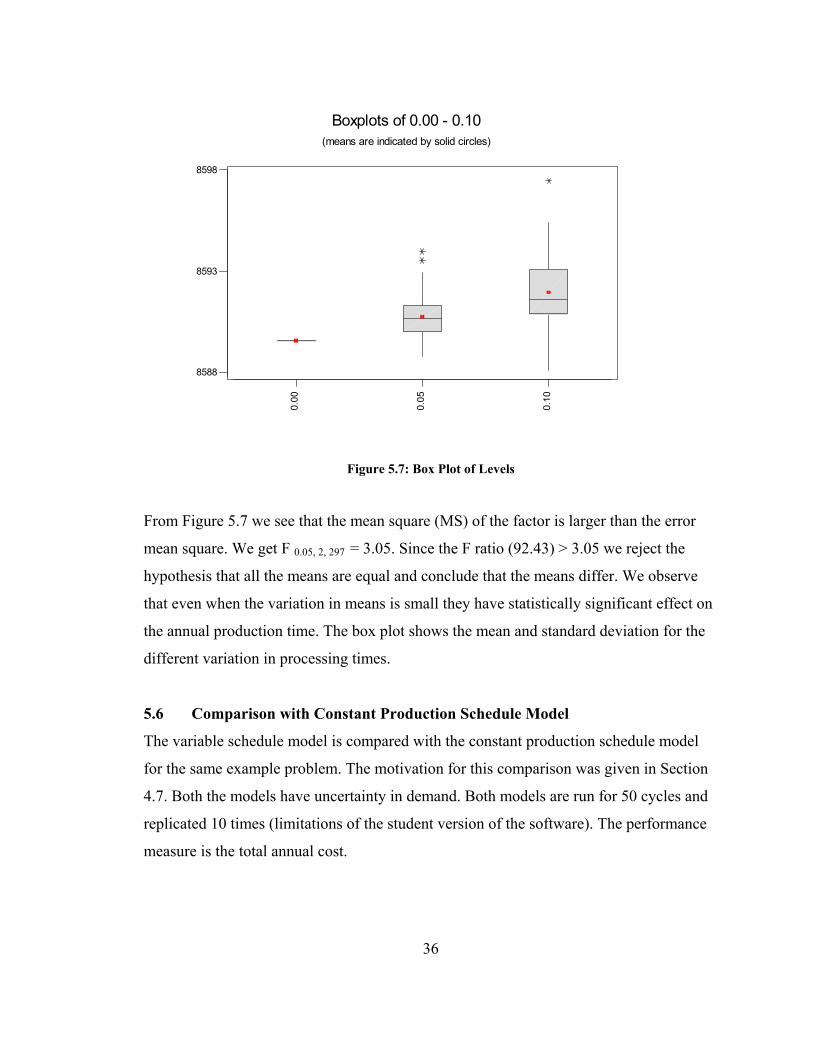
0.10
0.05
0.00
8598
8593
8588
Boxplots of 0.00 - 0.10(means are indicated by solid circles)
Figure 5.7: Box Plot of Levels
From Figure 5.7 we see that the mean square (MS) of the factor is larger than the error
mean square. We get F 0.05, 2, 297 = 3.05. Since the F ratio (92.43) > 3.05 we reject the
hypothesis that all the means are equal and conclude that the means differ. We observe
that even when the variation in means is small they have statistically significant effect on
the annual production time. The box plot shows the mean and standard deviation for the
different variation in processing times.
5.6 Comparison with Constant Production Schedule Model
The variable schedule model is compared with the constant production schedule model
for the same example problem. The motivation for this comparison was given in Section
4.7. Both the models have uncertainty in demand. Both models are run for 50 cycles and
replicated 10 times (limitations of the student version of the software). The performance
measure is the total annual cost.
36
5.6.1 Results and Analysis of Comparison
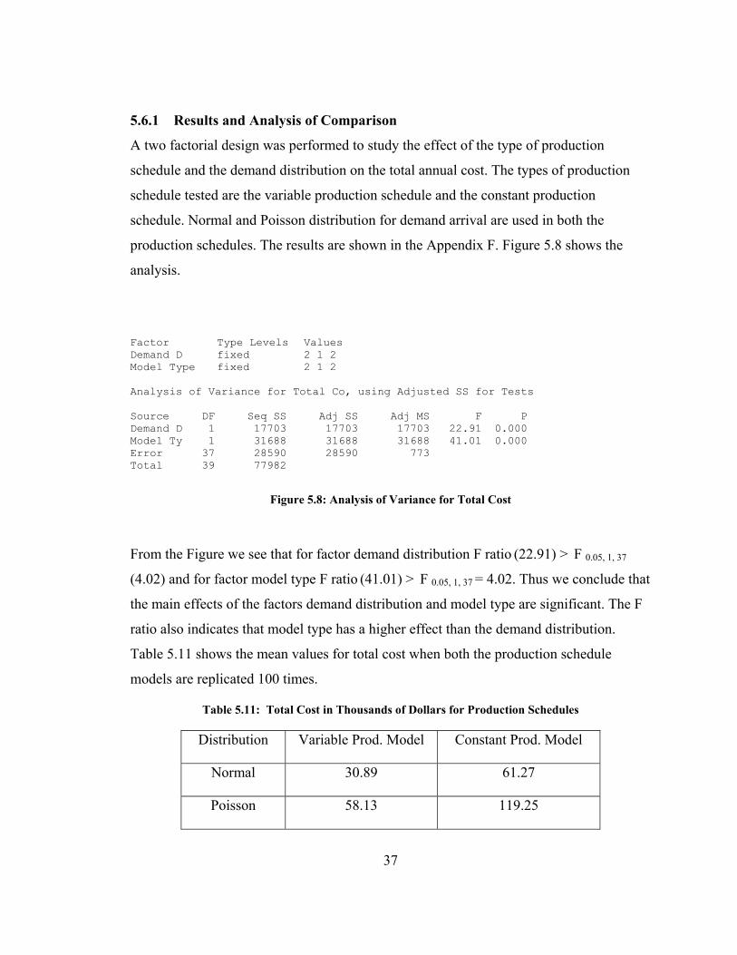
A two factorial design was performed to study the effect of the type of production
schedule and the demand distribution on the total annual cost. The types of production
schedule tested are the variable production schedule and the constant production
schedule. Normal and Poisson distribution for demand arrival are used in both the
production schedules. The results are shown in the Appendix F. Figure 5.8 shows the
analysis.
Factor Type Levels Values Demand D fixed 2 1 2 Model Type fixed 2 1 2 Analysis of Variance for Total Co, using Adjusted SS for Tests Source DF Seq SS Adj SS Adj MS F P Demand D 1 17703 17703 17703 22.91 0.000 Model Ty 1 31688 31688 31688 41.01 0.000 Error 37 28590 28590 773 Total 39 77982
Figure 5.8: Analysis of Variance for Total Cost
From the Figure we see that for factor demand distribution F ratio (22.91) > F 0.05, 1, 37
(4.02) and for factor model type F ratio (41.01) > F 0.05, 1, 37 = 4.02. Thus we conclude that
the main effects of the factors demand distribution and model type are significant. The F
ratio also indicates that model type has a higher effect than the demand distribution.
Table 5.11 shows the mean values for total cost when both the production schedule
models are replicated 100 times.
Table 5.11: Total Cost in Thousands of Dollars for Production Schedules
Distribution Variable Prod. Model Constant Prod. Model
Normal 30.89 61.27
Poisson 58.13 119.25
37
From Table 5.11 we observe that in the constant production schedule the uncertainty in
demand causes higher backorder and inventory accumulation compared to the variable
schedule model, thus resulting in higher total annual cost. The total cost is 98 % and
105 % higher when Normal and Poisson are used respectively as demand distributions.
Thus costs can be significantly reduced when demand uncertainties are taken into account
in the production schedule.
5.7 Summary
Several experiments were conducted to see the impact of demand uncertainty and
processing time variability. In the case of demand uncertainty the variability of the
distribution has a greater impact than the shape of the distribution on the total annual cost
comprising of backorder and inventory costs. The increase in annual production time
with higher variability was small but it was found to be statistically significant. Finally
the model with constant production schedule underestimates the average annual
backorder and inventory. The total annual cost in the constant production schedule was
considerably larger than the variable production schedule. The next chapter summarizes
the entire thesis and states the scope for future research.
38
CHAPTER 6
CONCLUSIONS AND FUTURE RESEARCH
6.1 Summary and Conclusions
A simulation model for a pharmaceutical batch plant producing four products was
developed using Arena simulation software. All the products required the same
processing steps. The production process had five stages, with parallel equipment in the
first and fourth stage. The bottleneck stage dictated the cycle time; therefore parallel units
were placed at the longest processing stages to minimize the cycle time. Zero wait
transfer policy and single product campaign with optimal sequence were assumed. The
batch sizes of all the products were assumed to be the same. A variable production
schedule was developed by incorporating uncertainties in demand and processing time
variability. Demand was assumed to arrive at the beginning of a planning period and
satisfied at the end of the period. Excess capacity in a planning period was utilized for
making inventory of products. If the demand could not be satisfied in a planning period
the excess demand was backordered. Attempts to solve a similar problem (unpaced
transfer line) using Markov chain were reported for only simplified cases based on
restrictive assumptions. An example problem was modeled using variable production
schedule with simulation as the tool. Cost was assigned to the average annual backorder
and inventory and was treated as a performance measure for the model.
Most of the literature for scheduling of multi-product batch plant does not include
demand uncertainties and processing time variability. A simulation model was also
developed for the same example problem where the production schedule is fixed. The
constant production schedule model had uncertain demand arrival, but the schedule was
independent of demand variations. If excess demand arrived in a planning period then it
39
was considered as backordered and if demand was insufficient compared to the constant
schedule then the product was made for inventory. Total cost for inventory and backorder
was set as the performance measure.
The effect of demand uncertainty on the total annual cost for the variable schedule
model was analyzed with different demand distributions. Analysis was performed for low
and high demand variability in order to see if the shape of the curve had a greater impact
or the variability. It was found that variability of the distribution had a significant effect
on the total annual cost. Higher the variability the higher was the cost. Sensitivity
analysis was performed to see the effect of different backorder to inventory cost ratios.
The difference in total annual costs persisted with different backorder to inventory cost
ratios for all the distributions.
Variability in processing times was analyzed with the annual production time as
the performance measure. The increase in annual production time with higher variability
was small but it was found to be statistically significant.
A two factorial design was performed to study the effect of the type of
production schedule and the demand distribution on the total annual. It was found that the
main effects of the factors demand distribution and model type are significant. The
constant production schedule in previous research underestimates the average annual
inventory and backorder. The total cost in variable schedule was found to be considerably
lower in comparison to the constant production schedule. Demand uncertainties have a
significant effect on the total annual cost and should be incorporated in the production
schedule.
6.1 Future Research
There are several extensions which have a scope for future research
1. In this research effect of demand uncertainty and processing time variability were
analyzed separately. A model can be developed where both; the demand and
processing time variability can be incorporated.
40
2. Zero wait policy was modeled in this research; however, it would be interesting to
analyze the effect of demand uncertainty and processing time variability on
inventory accumulation in a finite intermediate storage policy. Comparisons can
be made between zero wait policy and finite intermediate storage policy in terms
of increase in production capacity versus work in process requirements.
3. It is well known that use of in-process storage would reduce the cycle time and
increase the total production. A model can be developed for such a case to see the
increase in production in comparison to zero-wait policy when demand is
uncertain and processing times are variable.
41
REFERENCES
[1] Askin, R.G. and Standridge C.R. (1993) Modeling and Analysis of Manufacturing Systems. John Wiley and Sons, Inc.
[2] Balasubramanian, J. and Grossmann, I.E. (2002) “A Novel Branch and Bound Algorithm for Scheduling Flow-shop Plants with Uncertain Processing Times.” Comp. Chem. Eng., vol.26, pp.41.
[3] Balasubramanian, J. and Grossmann, I.E. (2000) “Scheduling to minimize expected completion time in flowshop plants with uncertain processing times.” Proc. ESCAPE-10, Elsevier, pp.79.
[4] Biegler, W.L.T., Grossmann, I.E. and Westerberg, A.W. (1997) Systematic Methods of Chemical Process Design Prentice Hall.
[5] Birewar, D.B. and Grossmann, I.E. (1990) “Simultaneous Synthesis, Sizing and Scheduling of Multiproduct Batch Plants.” Paper presented at AIChE Annual meeting, San Francisco, Ind. Eng. Chem. Res., vol. 29, pp. 2242-2251.
[6] Birewar, D.B. and Grossmann, I.E. (1989) “Incorporating Scheduling in the Optimal Design of Multi-products Batch Plants.” Comp. Chem. Eng., vol.13, pp. 307-315.
[7] Birewar, D.B. and Grossmann, I.E. (1989) “Efficient Optimization Algorithms for Zero-Wait Scheduling of Multiproduct Batch Plants.” Ind. Eng. Chem. Res., vol. 28, pp.1333-1345.
[8] Conway, R., Maxwell, W., McClain, J.O. and Thomas, L.J. (1988) “ The Role of Work-in Process Inventory in Serial Production Lines.” Operations Research, vol. 36(2), pp. 229-241.
[9] Fruit, W.M., Reklaitis, G.V. and Woods, J.M. (1974) “Simulation of Multiproduct Batch Chemical Processes” The Chemical Engineering Journal, vol 8, pp. 199-211.
[10] Graham, R.L., Lawler, E.L., Lenstra J.K. and Rinnooy Kan. A.H.G. (1979) “Optimization and Approximation in Deterministic Sequencing and Scheduling: A Survey.” Ann. Discrete Math., vol.5, pp. 287-326.
42
[11] Honkomp, S.J., Mockus, L. and Reklaitis, G.V. (1997) “Robust Scheduling with Processing Time Uncertainty.” Comp. Chem. Engg. vol. 21, pp.1055.
[12] Ierapetritou, M.G. and Pistikopoulos E.N. (1995) “Design of Multiproduct Batch Plants with Uncertain Demands” Comp. Chem. Eng., vol.19, pp 627 – 632.
[13] Ivanescu, C.V., Fransoo, J.C. and Bertrand, J.W.M. (2002) “Makespan Estimation and Order Acceptance in Batch Process Industries When Process Times are Uncertain.” OR Spectrum, vol. 24, pp. 467-495.
[14] Karimi, I.A. and Reklaitis, G.V. (1985) “Deterministic Variability Analysis for Intermediate Storage in Non Continuous Processes.” AIChE J., pp. 79.
[15] Kelton, W.D., Sadowski R.P and Sadowski, D.A. (1998) Simualtion with arena Mcgraw Hill.
[16] Knopf, F.C., Okos, M.R. and Reklaitis, G.V. (1982) “Optimal Design of Batch/Semi continuous Process.” Ind. Eng. Chem. Process. Des. Dev, vol. 1 pp. 76-86.
[17] Kuriyan, K. and Reklaitis, G.V. (1989) “Scheduling Network Flow-shops so as to Minimize Makespan.” Comp. Chem. Eng., vol. 13, pp. 187-200.
[18] Kuriyan, K., Joglekar, G. and Reklaitis, G.V. (1987) “Multi-product Plant Scheduling Studies using BOSS.” Ind. Eng. Chem. Res., vol. 26, pp.1551-1558.
[19] Miller, D.L. and Pekny, J.F. (1991) “Exact Solutions of Large Asymmetric Traveling Salesman Problem.” Science, vol. 225, pp. 754-761.
[20] Modi, A.K. and Karimi, I.A. (1989) “Design of Multi-product Batch Processes with Finite Intermediate Storage.” Comp. Chem. Eng., vol. 13, pp. 127-139.
[21] Petkov, S.B and Maranas, C.D. (1998) “Design of Single-Product Campaign Batch Plants under Demand Uncertainty.” AIChE Journal, Vol. 44, pp. 896-911.
[22] Petkov, S.B and Maranas, C.D. (1998) “Design of Multiproduct Batch Plants under Demand Uncertainty with Staged Capacity Expansions” Comp. Chem. Eng., vol.22, pp 789 – 792.
[23] Pistikopoulos, E.N., Thomaidis, T.V., Melin, A. and Ierapetritou, M.G. (1996) “Flexibility, Reliability and Maintenance Considerations in Batch Plant Design under Uncertainty.” Comp. Chem. Eng., vol. 16, pp. S1209-S1214.
[24] Reklaitis, G.V., Sunol, A.K., Rippin, D.W.T. and Hortacsu, O. (1992) Batch Processing Systems Engineering. Computer and Systems Sciences, vol. 143, Springer-verlag, New York.
43
[25] Rippin, D.W.T. (1983) “Simulation of Single and Multiproduct Batch Chemical Plants for Optimal Design and Operation.” ” Comp. Chem. Eng., vol. 7, pp 137 – 156.
[26] Sahinidis, N.V. and Grossmann, I.E. (1991) “MINLP Formulation for Cyclic Multiproduct Scheduling on Continuous Parallel Lines.” Comp. Chem. Eng., vol. 5(2), pp. 85-103.
[27] Straub, D.A. and Grossmann, I.E. (1992) “Evaluation and optimization of stochastic flexibility in multiproduct batch plants.” Comp. Chem. Eng., vol.16, pp 69-87.
[28] Voudouris, V.T. and Grossmann, I.E. (1991) “Mixed Integer Linear Programming Reformulations for Batch Process Design with Discrete Equipment Sizes.” Ind. Eng. Chem. Res., vol. 30, pp. 671-688.
[29] Voudouris, V.T. and Grossmann, I.E. (1993) “Optimal Synthesis of Multiproduct Batch Plants with Cyclic Scheduling and Inventory Considerations.” Ind. Eng. Chem. Res., vol.32, pp.1962-1980.
[30] Wellons, M.C. and Reklaitis, G.V. (1989) “Optimal Schedule Generation for A Single Product Production Line-1 Problem Formulation.” Comp. Chem. Eng., vol. 13(1/3), pp. 201-212.
[31] Yeh, N.C. and Reklaitis, G.V. (1987) “Synthesis and Sizing of Batch Semi Continuous Processes.” Comp. Chem. Eng., vol.6, pp. 639-654.
44
APPENDICES
45
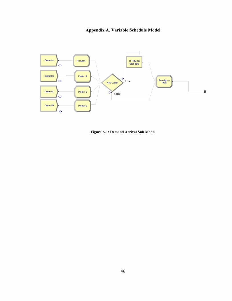
Appendix A. Variable Schedule Model
Demand A
Demand B
Demand C
Demand D
P roduct A
P roduct B
P roduct C
Product D
TimesReassigning
New Cycle? True
False
week doneTill Previous
0
0
0
0
0
0
Figure A.1: Demand Arrival Sub Model
46
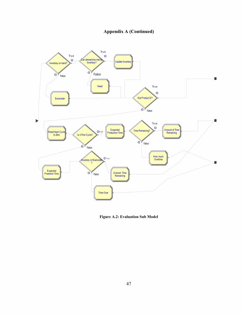
Appendix A (Continued)
Inventory on hand?
True
False
Inventory?Can demand be met by
True
False
Backorder
Need
Update Inventory
Not Product D?
True
False
to ZeroReset Next Cycle Time Remaining?
True
False
Is it First Cycle?T ru e
False
?Inventory or Backorder
T ru e
FalseProdction TimeExpected
Production TimeExpected
RemainingAmount of Time
OvertimeHow much
RemainingAmount Time
Time Over
0
0
0
0
0
0
0
0
0
0
0
0
Figure A.2: Evaluation Sub Model
47
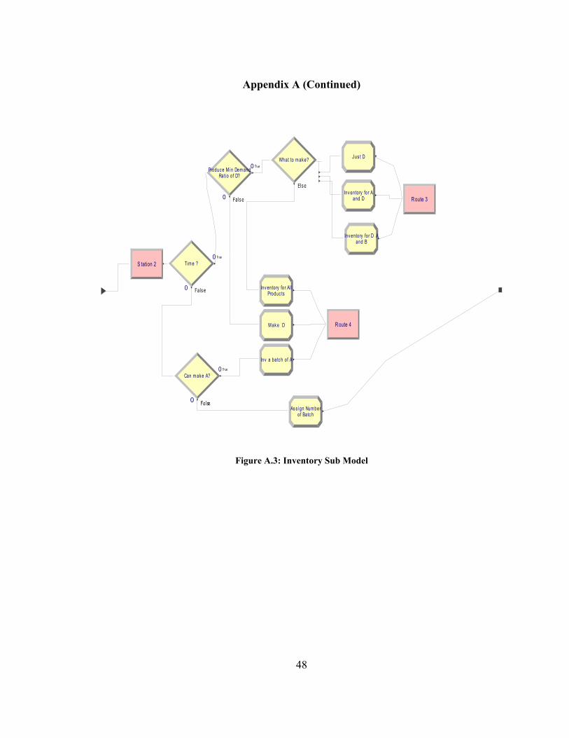
Appendix A (Continued)
and DInv entory for A
Ratio of D?Produc e M in Dem and
Tr ue
False
M ak e D
Else
What to m ak e? J us t D
Produc tsInv entory fo r Al l
and BInv entory for D A
Tim e ?Tr ue
False
of Batc hAs s ign Num ber
Can m ak e A?Tr ue
Fa lse
Inv a batc h of A
R oute 3
R oute 4
S tation 2
0
0
0
0
0
0
Figure A.3: Inventory Sub Model
48
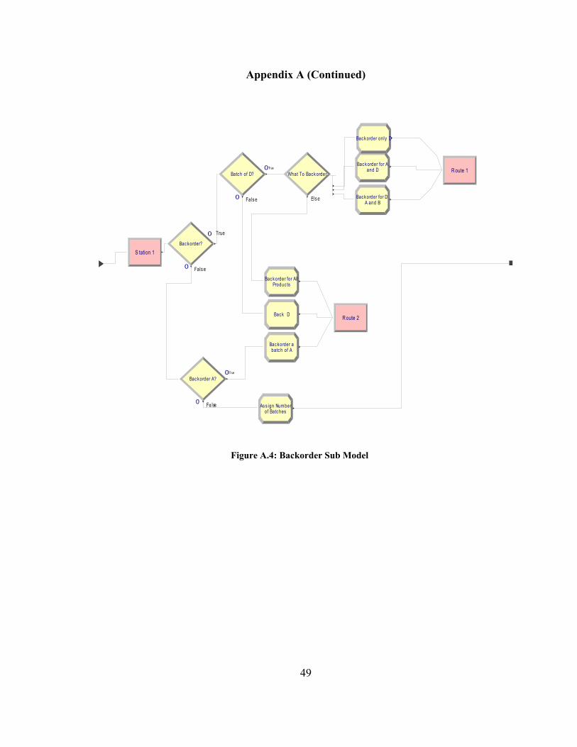
Appendix A (Continued)
Bac k order?
True
False
batc h of ABac k order a
Batc h of D?Tr ue
False Else
What To Bac k order
Bac k D
and DBac k order for A
Bac k order only D
A and BBac k order for D
Produc tsBac k order for Al l
o f Batc hesAs s ign Num ber
Bac korder A?Tr ue
Fa lse
S tation 1
R oute 1
R oute 2
0
0
0
0
0
0
Figure A.4: Backorder Sub Model
49
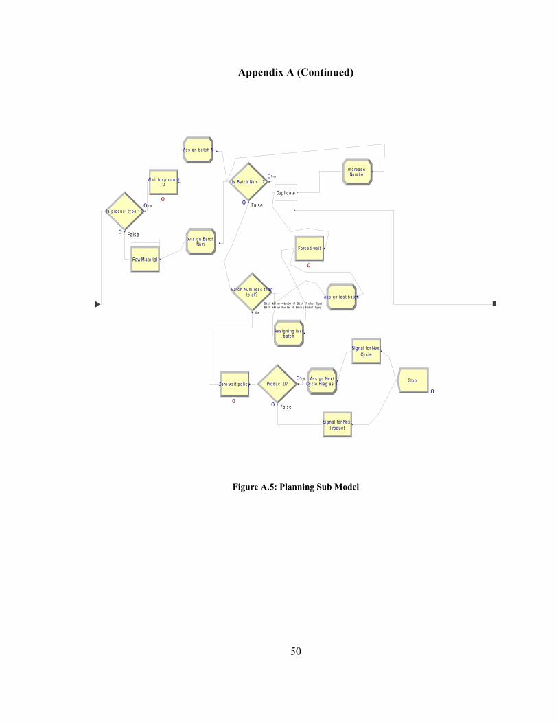
Appendix A (Continued)
Nu m b e rIn c re a s e
Nu mAs s i g n Ba tc h
1
Dupl ic ate
Is Ba tc h Nu m 1 ?Tr ue
False
to ta l ?Ba tc h Nu m l e s s th a n
Bat ch Num ber ==Num ber of Bat ch ( Pr oduct Type)Bat ch Num ber <Num ber of Bat ch ( Pr oduct Type)
Else
Fo rc e d wa i t
Is p ro d u c t ty p e 1 ?Tr ue
False
Raw M ateria l
Cy c leSignal for Nex t
Sto p
As s i g n l a s t b a tc h
b a tc hAs s i g n i n g l a s t
Ze ro wa i t p o l i c yTr ue
Fa ls e
Pro d u c t D? Cy c l e F l a g a s 1As s i g n Ne x t
Produc tSignal for Nex t
DW a i t fo r p ro d u c t
As s i g n Ba tc h N
0
00
0
0
0
0
0
0
0
Figure A.5: Planning Sub Model
50
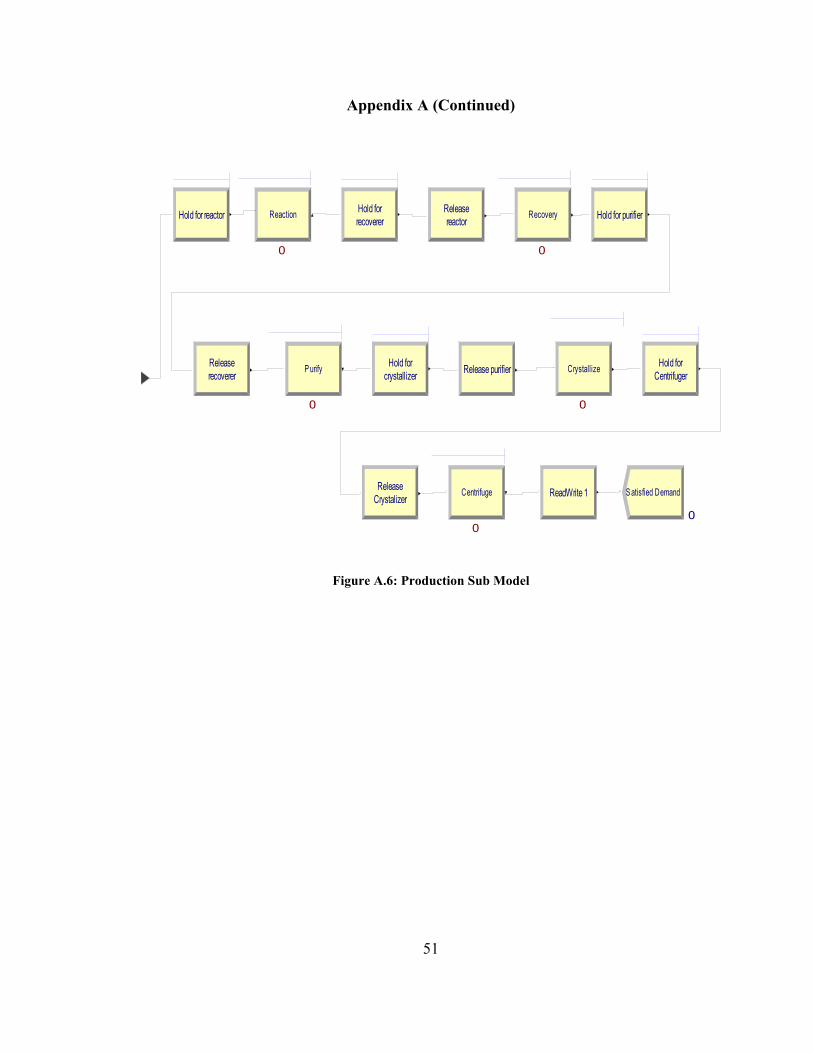
Appendix A (Continued)
Reaction Recovery
P urify Crystallize
Centrifuge S atisfied DemandReadWrite 1
recovererHold for
reactorRelease Hold for purifier
recovererRelease
crystallizerHold for Release purifier Centrifuger
Hold for
CrystalizerRelease
Hold for reactor
0
0 0
0 0
0
Figure A.6: Production Sub Model
51
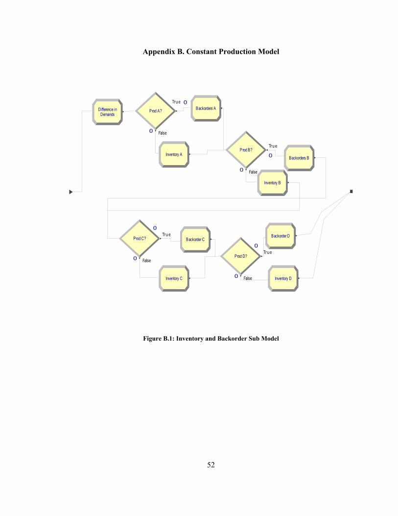
Appendix B. Constant Production Model
DemandsDifference in
True
False
Prod A?
Inventory A
Backorders A
Prod B?True
False
Backorders B
Inventory B
Prod C?True
False
Backorder C
Inventory C
Prod D?True
False
Backorder D
Inventory D
0
0
0
0
0
0
0
0
Figure B.1: Inventory and Backorder Sub Model
52
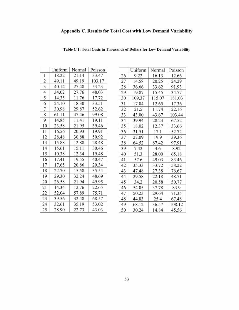
Appendix C. Results for Total Cost with Low Demand Variability
Table C.1: Total Costs in Thousands of Dollars for Low Demand Variability
Uniform Normal Poisson1 18.22 21.14 33.47 2 49.11 49.19 103.17 3 40.14 27.48 53.23 4 34.02 27.76 48.03 5 14.35 11.76 17.72 6 24.10 18.30 33.51 7 30.98 29.87 52.62 8 61.11 47.46 99.08 9 14.85 11.41 19.11 10 23.58 21.95 39.46 11 16.56 20.93 19.91 12 28.48 30.88 50.92 13 15.88 12.88 28.48 14 15.61 15.11 30.46 15 10.38 12.34 19.48 16 17.41 19.55 40.47 17 17.65 20.86 29.34 18 22.70 15.58 35.54 19 29.30 32.24 48.69 20 26.58 21.94 49.95 21 14.34 12.76 22.65 22 52.04 57.89 75.71 23 39.56 32.48 68.57 24 32.61 35.19 53.02 25 28.90 22.73 43.03
Uniform Normal Poisson 26 9.22 16.13 12.66 27 14.58 20.25 24.29 28 36.66 33.62 91.93 29 19.87 15.45 34.77 30 109.37 115.07 181.03 31 17.04 12.65 17.36 32 21.5 11.74 22.16 33 43.00 43.67 103.44 34 39.94 28.23 67.52 35 18.02 12.37 33.66 36 31.51 17.1 52.72 37 27.09 19.9 39.36 38 64.52 87.42 97.91 39 7.42 4.6 8.92 40 51.3 28.00 65.18 41 57.6 49.03 83.46 42 35.33 33.72 58.22 43 47.48 27.38 76.67 44 29.58 22.18 48.71 45 34.2 20.58 50.77 46 54.05 37.78 83.9 47 50.23 29.64 71.35 48 44.83 25.4 67.48 49 68.12 36.57 108.12 50 30.24 14.84 45.56
53
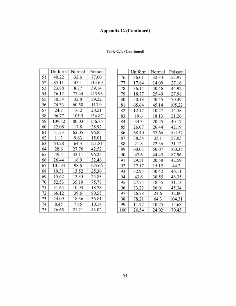
Appendix C. (Continued)
Table C.1: (Continued)
Uniform Normal Poisson51 40.22 32.6 77.00 52 85.11 45.1 114.69 53 23.88 8.77 39.14 54 76.12 77.44 175.95 55 30.34 32.8 59.22 56 74.33 60.58 113.9 57 24.7 16.2 20.21 58 96.77 105.5 134.87 59 109.52 80.03 156.75 60 22.08 17.8 28.92 61 51.73 62.05 96.85 62 11.3 9.63 15.01 63 64.28 64.3 121.81 64 28.6 27.76 42.52 65 49.5 42.11 96.25 66 26.44 16.9 32.46 67 101.93 98.6 195.66 68 19.31 13.52 25.36 69 15.62 12.35 25.83 70 52.53 35.19 75.78 71 31.64 10.93 18.78 72 66.12 39.6 80.55 73 24.09 18.36 36.81 74 8.45 7.85 10.14 75 26.65 21.21 43.02
Uniform Normal Poisson 76 36.01 32.34 57.97 77 17.84 14.00 27.16 78 36.14 40.46 44.92 79 18.77 25.49 27.98 80 50.18 40.45 70.49 81 65.64 45.14 105.22 82 12.17 10.27 14.58 83 19.6 18.13 21.26 84 34.3 20.25 40.17 85 26.07 20.44 42.19 86 68.40 57.66 104.57 87 38.54 33.1 57.03 88 21.8 22.36 31.12 89 60.03 50.07 100.35 90 47.6 44.45 87.96 91 29.51 20.58 42.59 92 37.17 15.12 44.2 93 32.95 30.42 46.11 94 43.6 30.55 48.35 95 27.75 18.55 31.13 96 33.22 26.01 45.34 97 26.78 24.6 32.00 98 78.21 64.3 104.31 99 11.77 10.25 15.68 100 26.54 24.02 70.43
54
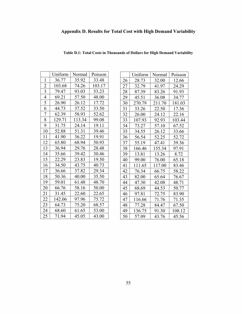
Appendix D. Results for Total Cost with High Demand Variability
Table D.1: Total Costs in Thousands of Dollars for High Demand Variability
Uniform Normal Poisson1 36.77 35.92 33.48 2 103.68 74.26 103.17 3 79.47 93.03 53.23 4 69.21 57.50 48.00 5 26.90 26.12 17.72 6 44.73 37.52 33.50 7 62.39 58.93 52.62 8 129.71 113.34 99.08 9 31.75 24.14 19.11 10 52.88 51.31 39.46 11 41.90 36.22 19.91 12 65.80 68.94 50.93 13 36.94 29.76 28.48 14 35.66 39.42 30.46 15 22.29 23.83 19.50 16 34.50 43.75 40.73 17 36.66 37.82 29.34 18 50.36 40.00 35.50 19 59.01 61.48 48.70 20 66.76 58.16 50.00 21 31.45 22.60 22.65 22 142.06 97.96 75.72 23 64.73 75.20 68.57 24 68.60 61.65 53.00 25 71.94 45.05 43.00
Uniform Normal Poisson 26 28.73 32.00 12.66 27 32.79 41.97 24.29 28 87.39 83.26 91.93 29 45.51 36.08 34.77 30 270.79 211.70 181.03 31 33.26 22.50 17.36 32 26.00 24.12 22.16 33 107.93 92.93 103.44 34 73.27 57.10 67.52 35 34.55 26.12 33.66 36 56.54 52.25 52.72 37 55.19 47.41 39.36 38 166.46 155.34 97.91 39 13.81 13.26 8.72 40 99.00 76.00 65.18 41 111.65 117.00 83.46 42 76.34 66.75 58.22 43 82.00 65.64 76.67 44 47.30 42.08 48.71 45 68.69 44.53 50.77 46 97.81 72.75 83.90 47 116.66 71.76 71.35 48 77.28 84.47 67.50 49 136.75 91.30 108.12 50 57.09 43.76 45.56
55
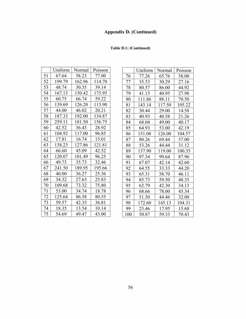
Appendix D. (Continued)
Table D.1: (Continued)
Uniform Normal Poisson51 67.64 58.23 77.00 52 199.79 162.96 114.70 53 48.74 30.35 39.14 54 167.13 150.42 175.95 55 60.75 66.74 59.22 56 139.69 126.20 113.90 57 44.00 46.02 20.21 58 187.33 192.00 134.87 59 259.11 181.50 156.75 60 42.52 36.43 28.92 61 104.92 117.00 96.85 62 17.81 16.74 15.01 63 138.23 127.86 121.81 64 66.60 45.09 42.52 65 120.07 101.49 96.25 66 49.73 35.73 32.46 67 241.50 189.95 195.66 68 40.00 36.27 25.36 69 34.32 27.63 25.83 70 109.68 73.32 75.80 71 53.00 34.74 18.78 72 125.64 86.58 80.55 73 59.57 42.35 36.81 74 18.35 13.54 10.14 75 54.69 49.47 43.00
Uniform Normal Poisson 76 77.26 65.76 58.00 77 35.53 30.29 27.16 78 80.57 86.00 44.92 79 41.15 40.95 27.98 80 111.86 88.11 70.50 81 143.14 117.50 105.22 82 30.44 29.00 14.58 83 40.93 40.58 21.26 84 68.04 49.00 40.17 85 64.93 53.00 42.19 86 151.08 126.00 104.57 87 80.26 69.44 57.00 88 53.26 44.44 31.12 89 137.90 119.00 100.35 90 97.34 99.64 87.96 91 67.07 42.14 42.60 92 64.55 33.33 44.20 93 65.31 58.70 46.11 94 85.73 59.50 48.35 95 62.79 42.30 34.13 96 68.66 78.00 45.34 97 51.50 44.46 32.00 98 172.60 145.13 104.31 99 23.46 17.95 15.68 100 50.87 59.33 70.43
56
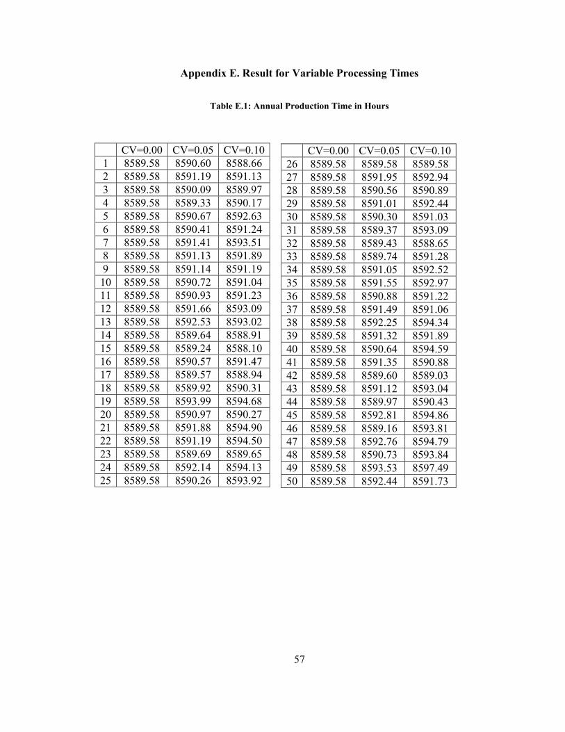
Appendix E. Result for Variable Processing Times
Table E.1: Annual Production Time in Hours
CV=0.00 CV=0.05 CV=0.101 8589.58 8590.60 8588.66 2 8589.58 8591.19 8591.13 3 8589.58 8590.09 8589.97 4 8589.58 8589.33 8590.17 5 8589.58 8590.67 8592.63 6 8589.58 8590.41 8591.24 7 8589.58 8591.41 8593.51 8 8589.58 8591.13 8591.89 9 8589.58 8591.14 8591.19 10 8589.58 8590.72 8591.04 11 8589.58 8590.93 8591.23 12 8589.58 8591.66 8593.09 13 8589.58 8592.53 8593.02 14 8589.58 8589.64 8588.91 15 8589.58 8589.24 8588.10 16 8589.58 8590.57 8591.47 17 8589.58 8589.57 8588.94 18 8589.58 8589.92 8590.31 19 8589.58 8593.99 8594.68 20 8589.58 8590.97 8590.27 21 8589.58 8591.88 8594.90 22 8589.58 8591.19 8594.50 23 8589.58 8589.69 8589.65 24 8589.58 8592.14 8594.13 25 8589.58 8590.26 8593.92
CV=0.00 CV=0.05 CV=0.10 26 8589.58 8589.58 27 8589.58 8591.95 8592.94 28 8589.58 8590.56 8590.89 29 8589.58 8591.01 8592.44 30 8589.58 8590.30 8591.03 31 8589.58 8589.37 8593.09 32 8589.58 8589.43 8588.65 33 8589.58 8589.74 8591.28 34 8589.58 8591.05 8592.52 35 8589.58 8591.55 8592.97 36 8589.58 8590.88 8591.22 37 8589.58 8591.49 8591.06 38 8589.58 8592.25 8594.34 39 8589.58 8591.32 8591.89 40 8589.58 8590.64 8594.59 41 8589.58 8591.35 8590.88 42 8589.58 8589.60 8589.03 43 8589.58 8591.12 8593.04 44 8589.58 8589.97 8590.43 45 8589.58 8592.81 8594.86 46 8589.58 8589.16 8593.81 47 8589.58 8592.76 8594.79 48 8589.58 8590.73 8593.84 49 8589.58 8593.53 8597.49 50 8589.58 8592.44 8591.73
8589.58
57
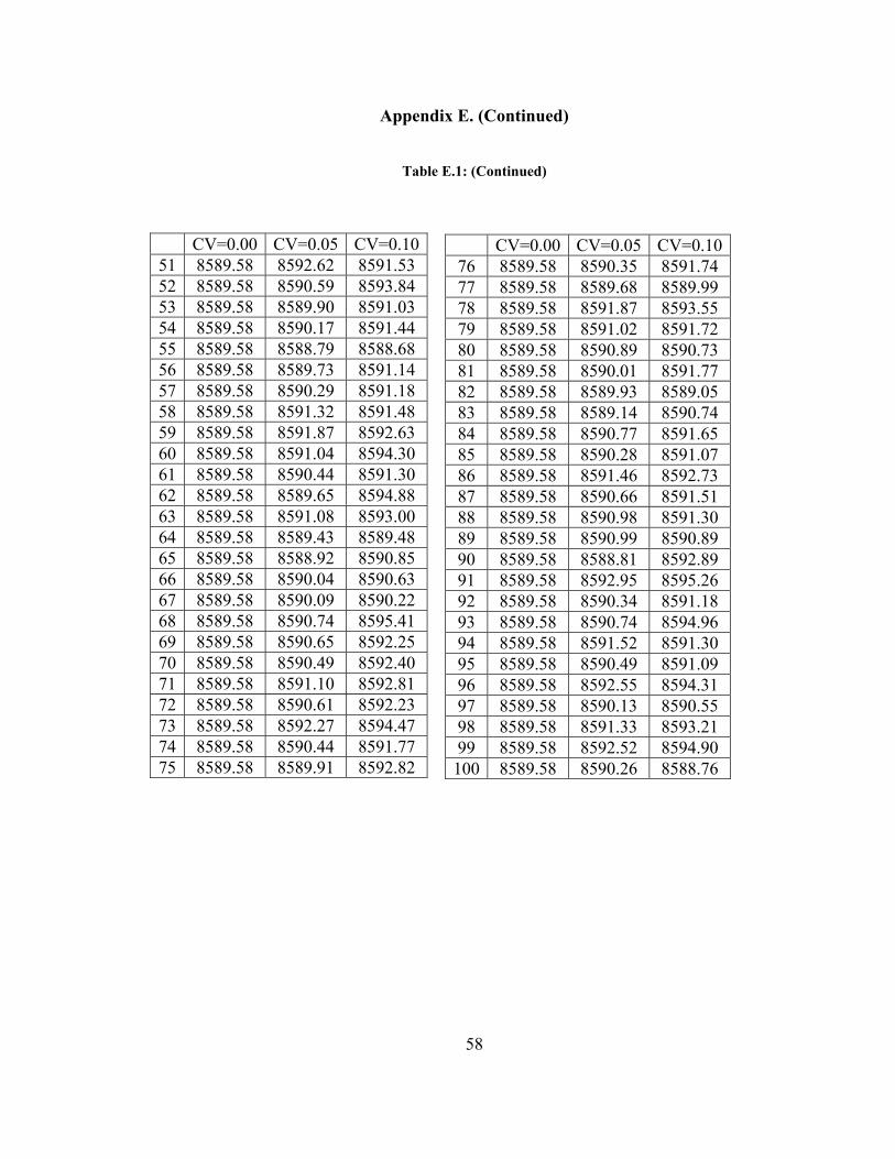
Appendix E. (Continued)
Table E.1: (Continued)
CV=0.00 CV=0.05 CV=0.1051 8589.58 8592.62 8591.53 52 8589.58 8590.59 8593.84 53 8589.58 8589.90 8591.03 54 8589.58 8590.17 8591.44 55 8589.58 8588.79 8588.68 56 8589.58 8589.73 8591.14 57 8589.58 8590.29 8591.18 58 8589.58 8591.32 8591.48 59 8589.58 8591.87 8592.63 60 8589.58 8591.04 8594.30 61 8589.58 8590.44 8591.30 62 8589.58 8589.65 8594.88 63 8589.58 8591.08 8593.00 64 8589.58 8589.43 8589.48 65 8589.58 8588.92 8590.85 66 8589.58 8590.04 8590.63 67 8589.58 8590.09 8590.22 68 8589.58 8590.74 8595.41 69 8589.58 8590.65 8592.25 70 8589.58 8590.49 8592.40 71 8589.58 8591.10 8592.81 72 8589.58 8590.61 8592.23 73 8589.58 8592.27 8594.47 74 8589.58 8590.44 8591.77 75 8589.58 8589.91 8592.82
CV=0.00 CV=0.05 CV=0.1076 8589.58 8590.35 8591.74 77 8589.58 8589.68 8589.99 78 8589.58 8591.87 8593.55 79 8589.58 8591.02 8591.72 80 8589.58 8590.89 8590.73 81 8589.58 8590.01 8591.77 82 8589.58 8589.93 8589.05 83 8589.58 8589.14 8590.74 84 8589.58 8590.77 8591.65 85 8589.58 8590.28 8591.07 86 8589.58 8591.46 8592.73 87 8589.58 8590.66 8591.51 88 8589.58 8590.98 8591.30 89 8589.58 8590.99 8590.89 90 8589.58 8588.81 8592.89 91 8589.58 8592.95 8595.26 92 8589.58 8590.34 8591.18 93 8589.58 8590.74 8594.96 94 8589.58 8591.52 8591.30 95 8589.58 8590.49 8591.09 96 8589.58 8592.55 8594.31 97 8589.58 8590.13 8590.55 98 8589.58 8591.33 8593.21 99 8589.58 8592.52 8594.90 100 8589.58 8590.26 8588.76
58
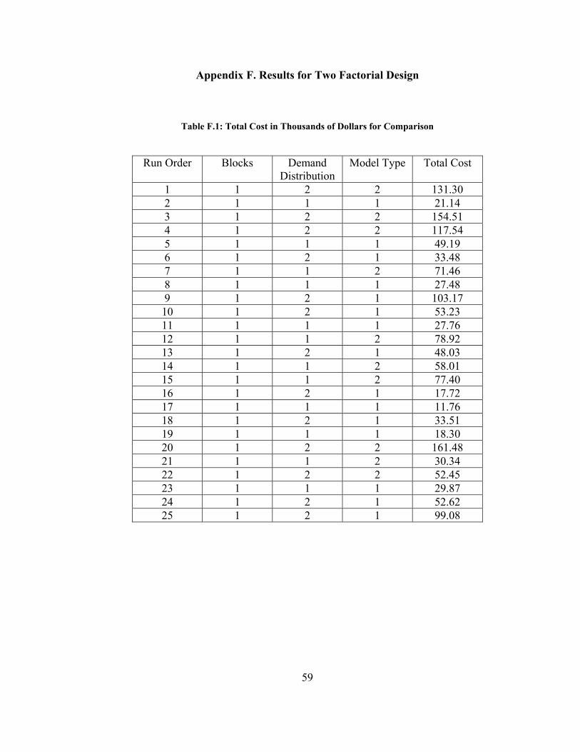
Appendix F. Results for Two Factorial Design
Table F.1: Total Cost in Thousands of Dollars for Comparison
Run Order Blocks Demand Distribution
Model Type Total Cost
1 1 2 2 131.30 2 1 1 1 21.14 3 1 2 2 154.51 4 1 2 2 117.54 5 1 1 1 49.19 6 1 2 1 33.48 7 1 1 2 71.46 8 1 1 1 27.48 9 1 2 1 103.17 10 1 2 1 53.23 11 1 1 1 27.76 12 1 1 2 78.92 13 1 2 1 48.03 14 1 1 2 58.01 15 1 1 2 77.40 16 1 2 1 17.72 17 1 1 1 11.76 18 1 2 1 33.51 19 1 1 1 18.30 20 1 2 2 161.48 21 1 1 2 30.34 22 1 2 2 52.45 23 1 1 1 29.87 24 1 2 1 52.62 25 1 2 1 99.08
59
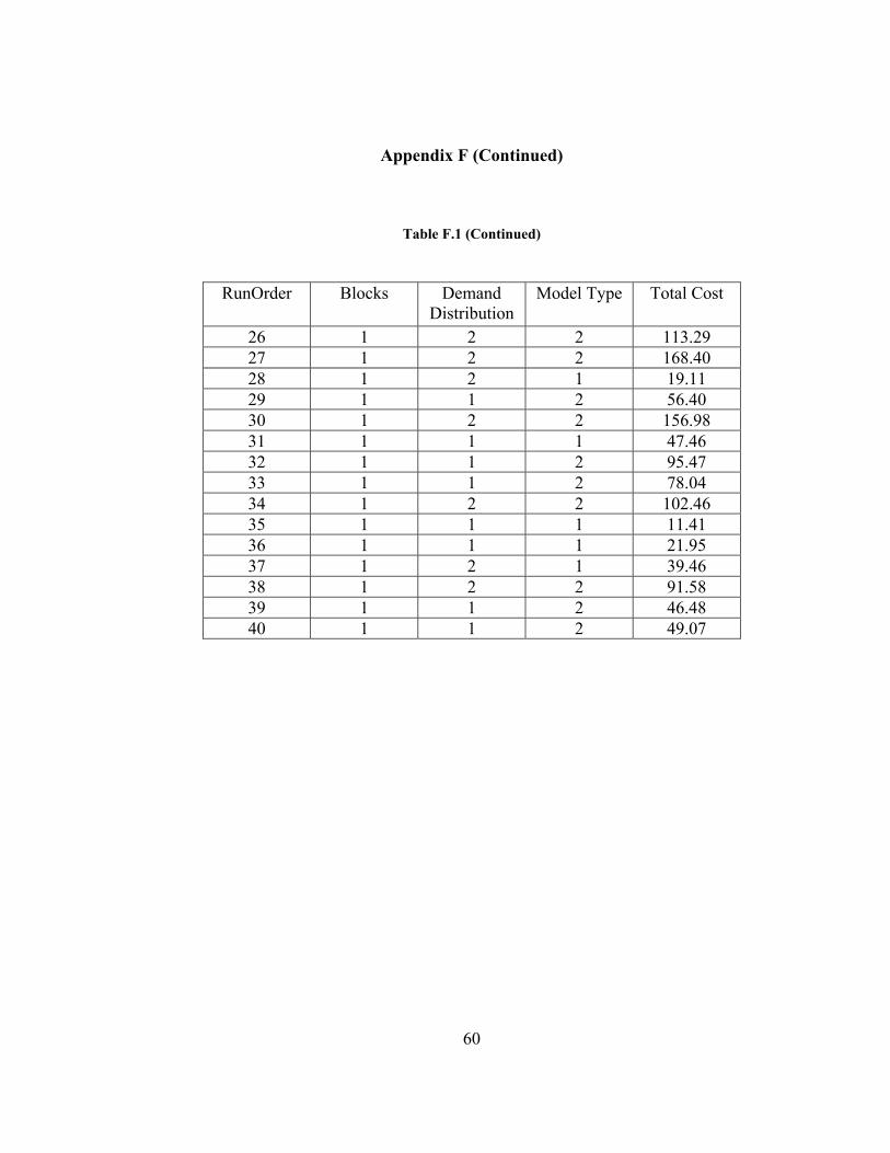
Appendix F (Continued)
Table F.1 (Continued)
RunOrder Blocks Demand Distribution
Model Type Total Cost
26 1 2 2 113.29 27 1 2 2 168.40 28 1 2 1 19.11 29 1 1 2 56.40 30 1 2 2 156.98 31 1 1 1 47.46 32 1 1 2 95.47 33 1 1 2 78.04 34 1 2 2 102.46 35 1 1 1 11.41 36 1 1 1 21.95 37 1 2 1 39.46 38 1 2 2 91.58 39 1 1 2 46.48 40 1 1 2 49.07
60