how importers may hedge demand uncertainty
TRANSCRIPT

How Importers May Hedge Demand Uncertainty
Horst Raff1
Nicolas Schmitt2
Frank Stahler3
June 14, 2018
We would like to thank Dennis Novy and seminar audiences for helpful comments andsuggestions. Financial support from SSHRC (Grant 435-2016-0354) is gratefully acknowledged.
1University of Kiel, Wilhelm-Seelig-Platz 1, D–24098 Kiel, Germany. Email: [email protected]
2Department of Economics, Simon Fraser University, Burnaby BC V5A 1S6, Canada. Email:[email protected] (Corresponding author)
3University of Tubingen, University of Adelaide, CESifo and NoCeT, Mohlstr. 36 (V4), D-72074 Tubingen, Germany. Email: [email protected]
Abstract
This paper examines how firms deal with demand uncertainty when importing interme-
diate goods takes time, and orders have to be placed before the realization of demand
is known. We consider two strategies to hedge this uncertainty: building up inventory of
imported goods, and relying on more expensive domestic supplies to cover peak demand.
Which strategy is optimal depends on the price of imported relative to domestic goods,
and on the degree of demand uncertainty. We also show that there are relative import
prices and degrees of demand uncertainty for which the firm chooses not to hedge uncer-
tainty and may thus stock out. The optimal hedging strategy implies a non-monotonic
relationship between firm-level output volatility and the relative import price.
JEL classification: F12, L81.
Keywords: International trade, dual sourcing, inventory, demand uncertainty, firm-level
output volatility

1 Introduction
It is by now well documented that the time required for goods to be shipped between coun-
tries and to clear customs represents a significant barrier to international trade (Hummels
and Schaur, 2013).1 This barrier is especially big for firms exposed to demand uncertainty,
since by the time goods arrive at their destination, the quantity shipped may no longer
be optimal. Consider, for instance, a firm that sources an input from abroad. Given the
delay associated with international trade, the firm has to order the input before knowing
the realization of demand. If demand turns out to be bigger than expected, the firm risks
a stockout, which may mean idling production capacity and/or foregoing profitable sales
opportunities. In case of lower-than-expected demand, the firm may accumulate stocks of
unused goods that may be costly to store or subject to depreciation or spoilage.
Several recent papers have explored strategies a firm engaged in international trade
may use to hedge demand uncertainty. Evans and Harrigan (2005), for instance, show that
retailers tend to source items subject to uncertain demand from nearby countries, even
if production costs there are higher than in alternative, more distant locations. Hummels
and Schaur (2010) explain that firms may resort to expensive but fast air shipments
to cover peak demand, while relying on slow but inexpensive ocean shipping for baseline
demand.2 Novy and Taylor (2014) argue that to protect against demand uncertainty firms
tend to keep much larger inventories of traded goods on hand than of domestically sourced
goods.3
In this paper we pursue a more general approach in which both dual sourcing as in
Hummels and Schaur (2010), and inventory buildup as in Novy and Taylor (2014) may
arise as special cases. We explore the firm’s optimal strategy choice in a model in which
the firm may source a homogeneous input good abroad or domestically. Import prices are
1Ocean shipping times between various ports around the world can be downloadedfrom several webpages, such as, https://www.searates.com/de/reference/portdistance orhttps://www.championfreight.co.nz/times.pdf. The World Bank provides information onthe time required for border and documentary compliance when goods are exported:http://www.doingbusiness.org/data/exploretopics/trading-across-borders.
2Strategies of this sort have been extensively analyzed in the operations management literature, wherethe are known as dual sourcing strategies. See Boute and Van Mieghem (2015) for a recent article andliterature review.
3See also Alessandria et al. (2010a, 2010b) on the need of firms to hold greater inventories of tradedthan of domestic goods.
1

lower than domestic prices, but imports have to be ordered before demand is known, and
they take one period to arrive; imports are hence the cheap, but inflexible source. Orders
for domestic goods can be placed after demand has been observed; domestic suppliers are
hence the flexible, but expensive source.4 When determining how much to produce, the
firm makes two decisions in every period. First, it decides whether to source inputs from
abroad and, if it does, how much to import knowing that these inputs take time to be
delivered. Second, it decides whether to source inputs domestically and, if so, how much
to buy knowing that these purchases can be used immediately. These decisions obviously
depend on the price difference between imported and domestic inputs, and they depend
on the degree of demand uncertainty on the output market. Not surprisingly, a firm facing
no uncertainty only chooses the cheaper source. The degree of uncertainty on the output
market is thus essential for choosing to simultaneously order from both the foreign and
the domestic source. Our model is simple enough to show that, as the imported input
becomes cheaper relative to the domestic input, for instance due to a reduction in trade
costs, the firm optimally sources a greater share of inputs from abroad for any given
level of demand uncertainty, and builds up an inventory of imported inputs. Once the
import price is sufficiently low, the firm finds it optimal to phase out domestic sourcing
altogether, and hedge demand uncertainty entirely through inventory build-up.
Why is this analysis important, and what does our approach allow us to demonstrate
that could not have been shown simply by considering each hedging strategy in isola-
tion? First, we can show that the response of imports and of inventory of imported goods
to a mean-preserving increase in demand uncertainty depends non-monotonically on the
price differential between imported and domestic inputs. Specifically, an increase in de-
mand uncertainty turns out to reduce imports and inventory when the price differential
is sufficiently small, but to increase imports and inventory when the price differential is
sufficiently big. This is because the firm relies more on domestic sourcing to hedge de-
mand uncertainty when the price differential is small, but more on inventory build-up
when the price differential is big. By allowing only one way to hedge demand uncertainty,
one may falsely conclude that an increase in demand uncertainty either reduces imports
and inventory (because the firm raises the share of domestically sourced inputs), or raises
4Alternatively both could be foreign with the difference coming from the mode of transportation(ocean shipping vs air shipping) as in Hummels and Schaur (2010) for exports, or one source being moredistant (China) than the other (Mexico) as in Evans and Harrigan (2005).
2

imports and inventory as the firm builds up its safety stock.
Second, we are able to show that the firm’s ability to adjust current output to demand
conditions, and thus firm-level output volatility, also depends non-monotonically on the
price differential between imported and domestic inputs and thus on the volume of im-
ports. If the price differential is small, the firm relies on domestic sourcing when demand
turns out to be high. Given that these inputs arrive immediately, the firm is able to adjust
output to demand shocks. If the price differential is big, the firm hedges against demand
shocks by building up its inventory of imported inputs. But with sufficient inventory on
hand, the firm is also able to adjust current output to demand conditions. For price dif-
ferentials in an intermediate range, the ability of firms to adjust output is limited. On
the one hand, the firm may find it too expensive to respond to a positive demand shock
by sourcing domestically. On the other hand, imported inputs are not cheap enough to
build up sufficient inventory to cover such demand shocks. Instead it may turn out to be
optimal for the firm to stock out, in which case output is completely independent of the
demand realization. Again, if we allow for only one way to hedge demand uncertainty,
we may wrongly conclude that there exists a monotonic relationship between firm-level
output volatility and the price differential, respectively the volume of imports.
The articles most closely related to ours are Hummels and Schaur (2010) and Novy
and Taylor (2014). Hummels and Schaur look at exports by air and by ocean shipping
(see also Aizenman, 2004). The firm in their model has to decide how best to hedge
demand uncertainty by determining how much to ship via ocean versus air transport,
and simulation results from the model are used to motivate an empirical study of the
link between the increased use of air shipping and the fall in the relative price of air
shipping. Their model, however, does not allow for inventory build-up, where the firm
carries over unsold goods into future periods. Thus greater demand uncertainty for a
good automatically leads to a greater share of air shipments. Moreover, for a given degree
of demand uncertainty, a negative contemporaneous demand shock tends to reduce air
shipments more than ocean shipments. In Novy and Taylor’s paper an input is either
imported or sourced domestically but not both. High-price domestic inputs arrive without
delay, but low-price imports arrive only with a time lag; hence the necessity in the case of
imported inputs to hedge demand uncertainty by building up inventory. A greater degree
of demand uncertainty in this model thus leads to a greater build-up of inventory, and a
contemporaneous negative demand shock hits imported inputs more than domestic inputs,
3

because firms first run down their inventories of imported inputs before re-ordering.
As already indicated above, our model can be viewed as encompassing both of these
strategies as special cases: dual sourcing from Hummels and Schaur (2010), and inventory
build-up from Novy and Taylor (2014). In particular, in our model, the choice between
sourcing an input domestically or from abroad is endogenous, as is the choice of how
much inventory to carry over into next period. In this way we are able to show that
which strategy a firm uses to hedge demand uncertainty depends on the price differential
between domestic and imported inputs. This implies that in our paper, the response to
changes in demand uncertainty and to contemporaneous demand shocks also depends on
this price differential.
Another novel aspect of our paper is that we examine what the use of different hedging
strategies implies for firm-level output volatility. How output (or employment) volatility
differs between trading and non-trading firms has recently received considerable attention
in the literature.5 Interest in this issue comes from the question whether trading firms
exhibit a different output or employment volatility than non-trading firms. Suppose, for
instance, they bring more volatility. Then, increased trade might harm risk-averse house-
holds by making their consumption patterns more volatile leading to lower welfare gains
from trade than predicted by standard trade models.6 The literature identifies two poten-
tial reasons why trading firms may exhibit a different volatility of output or employment
than non-trading firms: they may be exposed to foreign supply or demand shocks that
are imperfectly correlated with domestic shocks (e.g., Vannoorenberghe, 2012), or they
may react differently to domestic shocks than non-trading firms, or both (Buch et al.,
2009; Kurz et al., 2017). Our paper is linked to the latter strands of the literature, since it
deals with the ability of importers to hedge demand volatility and thus with their ability
to react to domestic shocks. Our contribution is to propose a microeconomic mechanism
linking imports to firm-level output volatility, whereas much of the existing literature
is either descriptive (e.g., Kurz and Senses, 2016) or relies on macroeconomic modelling
approaches (e.g., Kurz et al., 2017).7 The key insight we provide is that firm-level output
5See, for example, Kurz et al. (2017), Kurz and Senses (2016), Benz et al. (2016), Vannoorenberghe(2012), Buch et al. (2009). Industry-level studies are provided, for instance, by di Giovanni and Levchenko(2009).
6See, for instance, Newbery and Stiglitz (1984) for a general treatment of how trade may reduce socialwelfare in risky economies without insurance.
7See also Sundaram (2018) for a study examining the causal relationship between trade liberalization
4

volatility of importers may change non-monotonically with the price differential between
imported and domestic goods. In particular, we show that an increase in this price dif-
ferential, which goes hand in hand with an increase in international trade, may reduce
output volatility for low levels of the price differential and thus trade, but increase output
volatility for sufficiently high levels of the price differential and trade. This suggests that
empirical studies that assume a monotonic relationship between firm-level volatility and
trade may be misspecified.
The remainder of the paper is organized as follows. In the next section, we illustrate the
hedging strategies used by firms, in particular dual sourcing, using data for an anonymous
US steel wholesaler who relies both on importing and domestic sourcing for certain steel
products. We then propose a simple model consistent with this example in Section 3,
and derive the firm’s optimal inventory. In Section 4, we analyze the optimal hedging
strategy, and we show how inventory responds to changes in the price differential between
imported and domestic inputs and to changes in demand uncertainty. There we also
investigate what the optimal hedging strategy implies for firm-level output volatility.
Section 5 concludes by revisiting the example of the US steel wholesaler and confirming
that for two specific products, for which inventory data are available, the wholesaler’s
observed inventory investment strategies are consistent with our model’s predictions. In
the Appendix, we collect proofs of our results.
2 An Example of Dual Sourcing
Dual sourcing is illustrated by the case of an (anonymous) US steel wholesaler sourcing
products domestically and abroad.8 Among the steel products bought by this wholesaler,
we concentrate on the Hot Rolled Coil (HRC) product class.9 This class of products has
a total of 3,918 purchase transactions between July 1997 and November 2006 of which
1,952 (49%) are domestic, 1,274 (32%) are foreign, and the remaining 692 purchases
and firm volatility.8We thank George Hall for making the data available to us. The purchase transactions have also been
used by Alessandria et al. (2010a).9This class of steel products is typically used in construction, shipbuilding, and for large-size prod-
ucts such as tubes, gas containers, energy pipelines, etc. It should be distinguished from cold-rolled coilproducts that are typically more expensive and used for smaller/more precise products (automobiles forinstance).
5

0.0
05.0
1D
omes
tic d
ensi
ty
14000 15000 16000 17000Days
Domestic transactionsHCR products
0.0
05.0
1.0
15.0
2Fo
reig
n de
nsity
14000 15000 16000 17000Days
Foreign transactionsHCR products
Figure 1: HCR Transaction Density by Source
(19%) have unidentified origins.10 The HRC purchases are divided into 41 sub-products
depending on the thickness (the gauge) and the width (varying between 48 and 98 inches)
of the products.11 Every sub-product has both domestic and foreign purchases.
Figure 1 shows the daily frequency of domestic and foreign purchases over the 1997-
2006 sample period.12 It shows that dual sourcing is systematically taking place over the
period although the relative frequency of domestic and foreign purchases is not constant
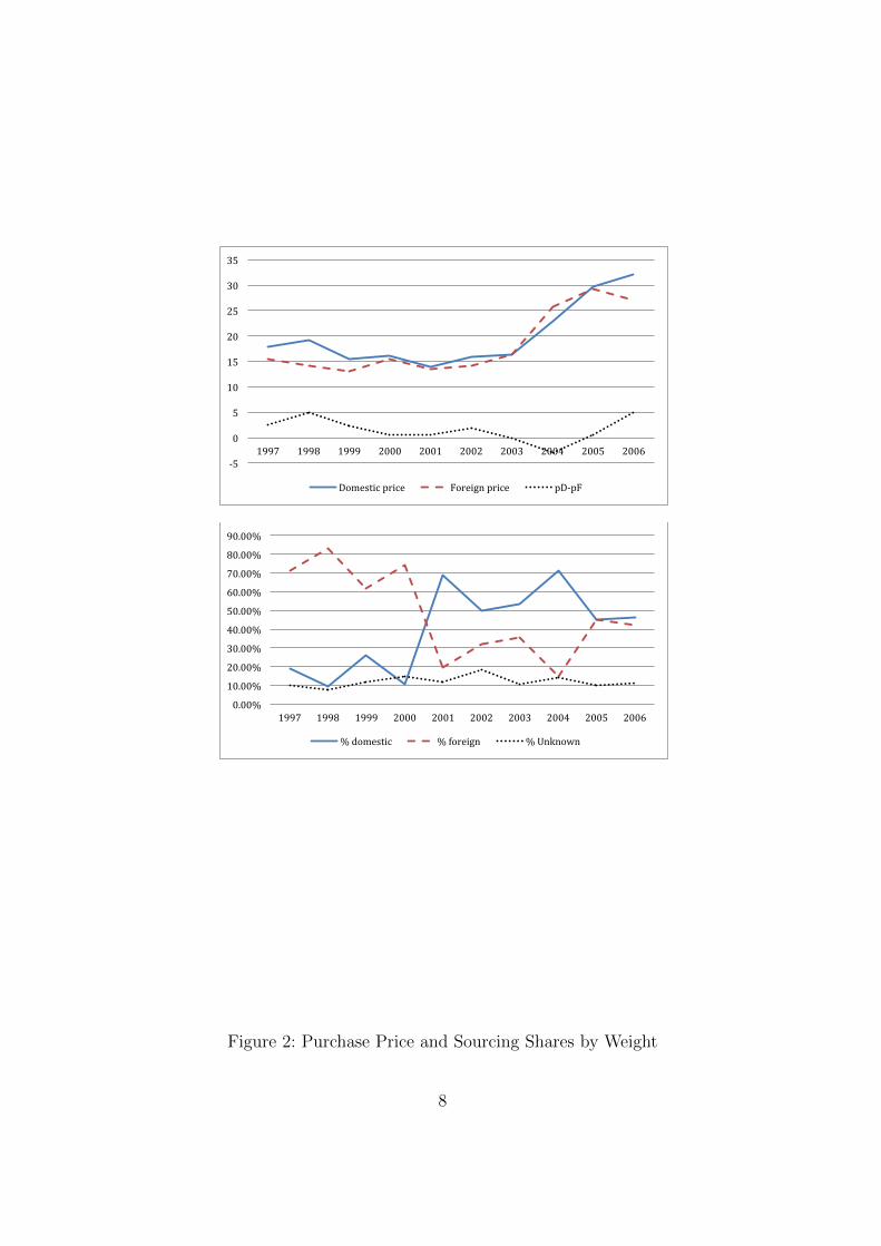
over time. Figure 2 shows the average domestic and foreign prices as well as the share of
domestic and foreign purchases (by weight) over the sample period. Notice that it is not
always the case that the domestic price is higher than the foreign price. This is especially
the case in 2000-03, which includes the period between March 20, 2002 and December 4,
2003 when the United States imposed Section 201-tariffs on 272 different 10-digit HS steel
products.13 Still, irrespective of which price is higher, it is still the case that both sources
10The name of the source countries is not known. We only observe whether a product is sourced abroador not. For each transaction, there is a date, product code, unit price, weight, and total amount paid.
11Two of these sub-products have less than 10 purchases and the top 28 sub-products represent about90% of the 3,918 transactions; the most purchased sub-product (HRC25048) represents 8% of the HRCpurchases.
12The transactions are missing during the period July-December 2004, the gap around 16,500 in Fig-ure 1.
13The temporary tariffs ranged from 8 to 30% depending on the steel products (compared to an average
6

are used (as Figure 2 illustrates) even if, as expected, the source with the lower price
commands the higher share. It is also interesting to note that the shift in market shares
in favor of domestic sourcing does not occur when the domestic price becomes lower than
the foreign price, but rather when the differential between the domestic and the foreign
price becomes low even if the foreign price is still lower, suggesting that the wholesaler is
willing to pay a premium on domestic purchases.
Table 1 shows that, on average, foreign prices are 13% lower than domestic prices
with very similar coefficients of variation indicating that the volatility of the domestic
and foreign prices is similar. Despite higher prices, domestic purchases represent 33% of
the total weight ordered. A critical difference between domestic and foreign purchases is
the average size of the orders with domestic orders amounting to about a third of the
average size of foreign orders. Associated with these different average orders is the fact
that domestic orders are more frequent than foreign orders. Computing the difference in
terms of the number of days between domestic orders (and separately between foreign
orders) for each sub-product (unweighted averages), the mean of the distribution is about
16 days between two consecutive domestic orders and about 28 days in between two
consecutive foreign orders. Moreover, the corresponding coefficient of variation is lower
for the foreign-order distribution (.49) than for the domestic-order one (.562).
Table 1: HRC product purchases
Origin Number Average CV Average CV Total sharepurchases price price Weight Weight by weight
Domestic 1,952 20.57 .362 88,312 .954 33%Foreign 1,274 17. 83 .359 223,232 1.135 55%
Unknown 692 18.53 .429 91,644 2.25 12%
Total 3,918 19.39 .381 132,478 1.42 100%
The example of this class of products shows that domestic purchases are frequent, small
and not regular, while foreign purchases are large, less frequent and show a somewhat
greater regularity. An explanation is that the foreign source is the primary and – on
tariff of 0 to 1% prior to the policy change) imposed on all but a handful of foreign sources (185 productsreceived a 30% tariff, 60 received a 15% tariff, 15 received a 13% tariff and 7 received an 8% tariff); seeBown (2013), Hufbauer and Goodrich (2003), Read (2005).
7
-‐5
0
5
10
15
20
25
30
35
1997 1998 1999 2000 2001 2002 2003 2004 2005 2006
Domestic price Foreign price pD-‐pF
0.00%
10.00%
20.00%
30.00%
40.00%
50.00%
60.00%
70.00%
80.00%
90.00%
1997 1998 1999 2000 2001 2002 2003 2004 2005 2006
% domestic % foreign % Unknown
Figure 2: Purchase Price and Sourcing Shares by Weight
8

average – cheaper source, but foreign purchases take time to arrive. Domestic orders are
delivered immediately but are more expensive on average, and are thus not used all the
time. In the following section, we propose a simple model consistent with this explanation.
3 The Model
Consider a firm facing the inverse linear demand pt = a + εt − bqt for its product in
period t, where εt is a random shock uniformly distributed according to the c.d.f. F (εt) =
(εt + ∆)/2∆, qt denotes output in period t, and ∆ < a holds such that the random shock
is small relative to the size of the market. For each unit of output, the firm needs one
unit of a homogeneous input that it can obtain from two possible sources: a domestic
source or a foreign source. Domestic sourcing is immediate in the sense that inputs can
be ordered and delivered after the demand in that period has been revealed; hence we
may think of domestic orders as involving just-in-time delivery. The domestic order in
period t is associated with the domestic unit cost wt and quantity yt. Foreign sourcing is
inflexible, because an order has to be placed before the realization of demand is known,
and it takes time for that order to be delivered. In particular, an input purchase made
(and paid) in period t− 1, at the foreign unit cost vt−1 and involving a quantity denoted
by mt−1, can only be used in production in period t or later. We interpret the unit input
cost as including the unit price as well as transport and other transaction costs involved
in purchasing the input. In the case of the foreign unit cost, these other costs will typically
include import tariffs, customs clearing costs, insurance, etc. We may therefore think of
a decrease in the foreign unit cost as reflecting a decrease in trade costs. Since domestic
and foreign inputs used in a given period are not bought during the same period, we take
into account the discount factor, δ < 1, so that, at time t, the appropriate comparison of
the two input costs is wt and vt−1/δ. We consider the case where the foreign, inflexible
source is cheaper than the domestic, flexible source (i.e., wt ≥ vt−1/δ).
The trade-off between the two sources is clear: the foreign source is relatively cheap
but it forces a firm to commit to it before demand is known and it can only be used in
production next period, whereas the domestic source is relatively expensive but ‘imme-
diate’ in the sense that an order can be placed and received once the current demand is
known. In any period, the firm may end up not using the entire quantity of inputs that it
purchased. We denote the volume of these unsold units in period t by z0t and they become
9

part of the available inputs to be used in t+ 1. We refer to z0t as the excess inventory (or
inventory build-up). It turns out to be analytically convenient to assume that the firm
attaches an exogenous and constant value ρt > 0 to each of these units.14 We make the
further assumption that ρt < vt−1/δ ≤ wt. Thus, while the firm places a positive value
on unsold units, this value is not so high that it would voluntarily accumulate excess
inventory.15 We let zt denote total inventory in period t and define it as the volume of
inputs available for use at the beginning of the period. Thus total inventory is equal to
zt = mt−1 + z0t−1, that is, the sum of imports purchased in period t−1 and arriving at the
beginning of period t, and the excess inventory inherited from period t − 1. We assume
that z0t−1 is known when the firm chooses mt−1.16 The cost of storing inventory between
periods is normalized to zero.
It must be clear from above that, at the beginning of a period, the cost of the foreign
inputs is sunk whereas the cost of domestic inputs is avoidable. Thus, a firm always prefers
using its entire available inventory before buying from the domestic source so that, in any
period, it faces three possibilities: (i) it uses less than its inventory zt and does not order
from the domestic source; (ii) it uses its entire inventory but does not order from the
domestic source; or (iii) it uses its entire inventory and buys, as well as uses, yt from the
domestic source.
To make this more precise, consider a firm’s profit denoted by πt(qt):
πt(qt) =
{(a+ εt − bqt)qt + ρt(zt − qt) if qt ≤ zt,
(a+ εt − bqt)qt − wt(qt − zt) if qt > zt.(1)
The optimal output in t is therefore given by:
q∗t (εt) =
a+εt−ρt
2bif a+εt−ρt
2b≤ zt,
zt if a+εt−wt
2b< zt <
a+εt−ρt2b
,a+εt−wt
2bif a+εt−wt
2b≥ zt.
(2)
14We discuss the case where ρt is endogenously determined in Appendix A.5.15Our model could easily accommodate the case where ρt > vt−1/δ, but this is not the focus of our
paper.16This implies in particular that, when a foreign order is placed, the firm knows the realization of the
demand of the current period.
10
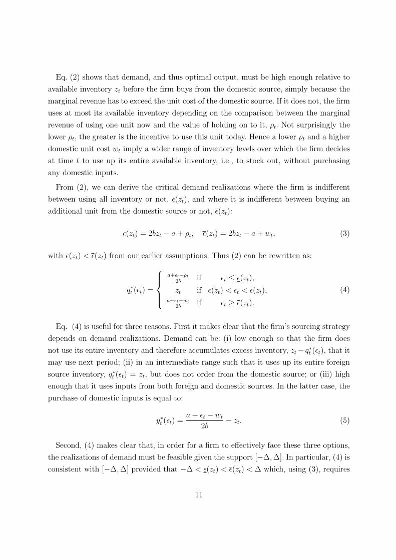
Eq. (2) shows that demand, and thus optimal output, must be high enough relative to
available inventory zt before the firm buys from the domestic source, simply because the
marginal revenue has to exceed the unit cost of the domestic source. If it does not, the firm
uses at most its available inventory depending on the comparison between the marginal
revenue of using one unit now and the value of holding on to it, ρt. Not surprisingly the
lower ρt, the greater is the incentive to use this unit today. Hence a lower ρt and a higher
domestic unit cost wt imply a wider range of inventory levels over which the firm decides
at time t to use up its entire available inventory, i.e., to stock out, without purchasing
any domestic inputs.
From (2), we can derive the critical demand realizations where the firm is indifferent
between using all inventory or not, ε(zt), and where it is indifferent between buying an
additional unit from the domestic source or not, ε(zt):
ε(zt) = 2bzt − a+ ρt, ε(zt) = 2bzt − a+ wt, (3)
with ε(zt) < ε(zt) from our earlier assumptions. Thus (2) can be rewritten as:
q∗t (εt) =
a+εt−ρt
2bif εt ≤ ε(zt),
zt if ε(zt) < εt < ε(zt),a+εt−wt
2bif εt ≥ ε(zt).
(4)
Eq. (4) is useful for three reasons. First it makes clear that the firm’s sourcing strategy
depends on demand realizations. Demand can be: (i) low enough so that the firm does
not use its entire inventory and therefore accumulates excess inventory, zt− q∗t (εt), that it
may use next period; (ii) in an intermediate range such that it uses up its entire foreign
source inventory, q∗t (εt) = zt, but does not order from the domestic source; or (iii) high
enough that it uses inputs from both foreign and domestic sources. In the latter case, the
purchase of domestic inputs is equal to:
y∗t (εt) =a+ εt − wt
2b− zt. (5)
Second, (4) makes clear that, in order for a firm to effectively face these three options,
the realizations of demand must be feasible given the support [−∆,∆]. In particular, (4) is
consistent with [−∆,∆] provided that −∆ < ε(zt) < ε(zt) < ∆ which, using (3), requires
11

that ε(zt) − ε(zt) = wt − ρt < 2∆. Hence, given wt and ρt, (4) requires a relatively high
degree of demand uncertainty.
Third, it makes it easy to characterize graphically the possible cases that may arise.
Figure 3, where [ε(zt), ε(zt)] is fully contained in [−∆,∆], illustrates the possible real-
izations of demand consistent with (4). If the demand uncertainty is low as in Figure 4,
however, and thus if [−∆,∆] is fully contained in [ε(zt), ε(zt)], then the firm’s optimal
output can only be q∗t (εt) = zt irrespective of the realization of demand.
−∆ ∆
ε ε
Figure 3: High demand uncertainty
−∆ ∆
ε ε
Figure 4: Low demand uncertainty
We can now proceed to the determination of optimal inventory z∗t . Notice that the
cases illustrated by Figures 3 and 4 are just two possible outcomes among several that
we have to examine. Going through all of these cases is obviously repetitive. So we show
only one case here and refer the reader to Appendix A.1 for a derivation of the optimal
inventory in the other cases. We focus on the case in which the firm’s expected marginal
revenue in period t is consistent with the optimal output q∗t as provided by (4) and thus
for realizations of demand consistent with Figure 3. The expected marginal revenue in
period t, E [MRt], from a unit of input sourced from abroad in period t− 1 is equal to:
δE [MRt] = δ
[∫ ε(zt)
−∆
ρtdεt2∆
+
∫ ε(zt)
ε(zt)
(a+ εt − 2bzt)dεt2∆
+
∫ ∆
ε(zt)
wtdεt2∆
]. (6)
The marginal revenue is equal to ρt for low demand realizations (−∆ ≤ εt ≤ ε(zt)) and
thus when the firm holds on to units for the next period. It is equal to a + εt − 2bzt
when the entire inventory zt is used, and is equal to wt when the demand realizations are
12

sufficiently high (ε(zt) ≤ εt ≤ ∆) that purchasing from the domestic source is required.
Using (3) to evaluate (6), equating the outcome to the foreign price vt−1, and solving for
zt, we obtain as optimal inventory:
z∗t,123 =2a− (wt + ρt)
4b+
∆(wt + ρt)
2b(wt − ρt)− ∆vt−1/δ
b(wt − ρt). (7)
Here z∗t,123 denotes the optimal inventory in regime (123), in which all three ranges of
demand realizations are feasible: building up inventory due to a low demand realization
(labeled range 1), using up total inventory but without any domestic sourcing (labeled
range 2), and using up total inventory and sourcing additional inputs domestically (labeled
range 3). In what follows, the subscript will denote the relevant regime, i.e., the feasible
range(s).
Other regimes are possible, all involving a subset of the three ranges of demand realiza-
tions. Thus, z∗t,23 (valid for ε(z∗t,23) < −∆ < ε(z∗t,23) < ∆) refers to the optimal inventory
which is always fully used but with some demand realizations requiring domestic sourc-
ing; z∗t,12 (valid for −∆ < ε(z∗t,12) < ∆ < ε(z∗t,12)) is the optimal inventory when domestic
sourcing never takes place and where the available inventory might not be entirely used.
Finally, z∗t,2 (valid for ε(z∗t,2) < −∆ and ε(z∗t,2) > ∆) is the optimal inventory when it is
always entirely used and no domestic sourcing takes place (illustrated by Figure 4).
Lemma 1 summarizes results derived in Appendix A.1.
Lemma 1. 1. In addition to z∗t,123, the feasible inventory levels are:
z∗t,2 =a− vt−1/δ
2b; z∗t,12 =
a+ ∆− ρt − 2√
∆ (vt−1/δ − ρt)2b
;
z∗t,23 =a− wt −∆ + 2
√∆(wt − vt−1/δ)
2b.
2. The conditions under which z∗t,2 and z∗t,123 hold are mutually exclusive.
3. Two inventory levels are not feasible: z∗t,1 and z∗t,3.
Proof. See Appendix A.1.
Two comments are in order. First, two cases never arise: z∗t,1 when inventories always
exceed needs (requiring ε(z∗t,1) > ∆), and z∗t,3 involving systematic domestic sourcing
13

irrespective of demand realizations (requiring ε(z∗t,3) < −∆). The former would imply
a permanent inventory build-up, which is not an equilibrium strategy in our model: a
firm never systematically chooses to order so much from abroad that it would build up
inventory for any demand realization. The latter would imply that a firm always sources
at least some inputs at home for any demand realization, even if vt−1/δ < wt.17 Second,
the conditions under which z∗t,123 and z∗t,2 hold are mutually exclusive because they do not
depend on the foreign price but only on the comparison of the degree of uncertainty (2∆)
with (wt − ρt), with z∗t,123 requiring 2∆ > wt − ρt, and z∗t,2 requiring 2∆ < wt − ρt.
4 The Optimal Hedging Strategy
We are now ready to determine how a change in the foreign unit cost, vt−1/δ, as might
result from a change in trade costs, and a change in the level of uncertainty affect the firm’s
optimal hedging strategy and thus its imports. It turns out to be analytically convenient
to focus on determining how changes in the foreign unit cost and uncertainty affect z∗t and
thus the optimal ‘stock’ of inventory rather than the ‘flow’ of imports, m∗t−1, as is typically
done in trade analysis. This is legitimate because the two concepts are closely connected.
In particular, the optimal import quantity in period t− 1, m∗t−1, is equal to the difference
between the optimal inventory the firm wants to hold at the beginning of period t, z∗t ,
and the excess inventory accumulated in t− 1, z0t−1. Hence m
∗t−1 = z∗t − z0
t−1. Given that
z0t−1 is known when the firm chooses how much to order from abroad, determining m
∗t−1
is equivalent to choosing z∗t .18 The advantage of picking inventory as our unit of analysis
rather than imports is that it avoids having to track unsold units inherited from earlier
periods without modifying the results. Its only drawback is that it may be less amenable
to empirical analysis, as the inventory of imported goods is typically less easily observable
than imports.
Consider the effect of a decrease in the foreign unit cost. We observe that the optimal
inventory levels in the different regimes summarized in Lemma 1 all rise monotonically
as the foreign cost decreases (i.e., ∂z∗t /∂(vt−1/δ) < 0). However, we have to take into
17In Appendix A.1, we show that domestic sourcing becomes the primary and only source (i.e. z∗t,3 = 0)if vt−1/δ > wt.
18If orders were placed before z0t−1 is known, then m∗
t−1 = z∗t −E(z0t−1), where E(z0t−1) is the expectedexcess inventory.
14

account that, as the foreign unit cost decreases, the inventory regime will switch. To see
this, observe that ε(zt) − ε(zt) = wt − ρt is independent of vt−1/δ, but ε(zt) and ε(zt) do
depend on vt−1/δ. In particular, given (3),
∂ε(zt)
∂(vt−1/δ)=
∂ε(zt)
∂(vt−1/δ)= 2b
∂zt∂(vt−1/δ)
< 0, (8)
so that graphically a reduction in the foreign unit cost shifts the interval ε(zt) − ε(zt) =
wt−ρt from left to right relative to a fixed range of length 2∆ centered around zero. This
implies two separate inventory regime paths: one conditional on ε(zt)−ε(zt) = wt−ρt < 2∆
(see Figure 5) and the other conditional on ε(zt) − ε(zt) = wt − ρt > 2∆ (see Figure 6).
In particular, if 2∆ > ε(zt) − ε(zt) = wt − ρt, there is a unique path from regime (3)
to regime (23) to regime (123) to regime (12) with z∗t,3 = 0 ≤ z∗t,23 ≤ z∗t,123 ≤ z∗t,12. If
2∆ < ε(zt) − ε(zt) = wt − ρt, there is a unique path from regime (3) to regime (23) to
regime (2) to regime (12) with z∗t,3 = 0 ≤ z∗t,23 ≤ z∗t,2 ≤ z∗t,12.
lower vt−1/δ−∆ ∆
ε ε
ε ε
ε ε
Regime (12)
Regime (123)
Regime (23)
Figure 5: Trade liberalization path with high demand uncertainty
Consider the first path and assume that the foreign price is sufficiently high that
vt−1/δ ≥ wt. Clearly, a firm sources domestically only and there is no foreign sourcing
irrespective of the realization of demand. This case corresponds to z∗t,3 = 0. When lower
foreign prices bring wt > vt−1/δ, the first possible bound to intersect the fixed range 2∆
is ε(zt). This implies that z∗t,23 is the first possible optimal inventory level consistent with
foreign sourcing. Since in this regime foreign sourcing is not much cheaper than domestic
15

lower vt−1/δ−∆ ∆
ε ε
ε ε
ε ε
Regime (12)
Regime (2)
Regime (23)
Figure 6: Trade liberalization path with low demand uncertainty
sourcing, the firm relies on domestic sourcing to buffer large positive demand shocks. In
the case of low demand shocks, the firm chooses to stock out rather than to be left with
unsold inventory at the end of the period. Lower foreign unit costs lead the lower bound
of ε(zt)− ε(zt) to intersect the fixed range 2∆ so that z∗t,123 becomes the optimal inventory
level. Now, in addition to purchasing domestically when demand turns out to be very
high, the firm acquires so much inventory that it is stuck with unsold inventory should
demand turn out to be very low. Still lower foreign unit costs imply that ε(zt) exceeds ∆
which leads to z∗t,12 as the only possible optimal inventory level. In this case, the foreign
unit cost is so low compared to the domestic cost that the firm never sources domestically.
It stocks out if demand turns out to be high and accumulates inventory when demand
happens to be low. The second possible path is the same as the first one except that, since
2∆ < ε(zt)− ε(zt) = wt− ρt, the optimal inventory level z∗t,123 never arises but is replaced
by z∗t,2 instead, which is the optimal inventory when the firm prefers to stock out rather
than to source domestically or to carry unsold units into the subsequent period.
We prove in Appendix A.2 that, at the foreign-unit-cost levels at which these regime
switches occur, inventory is continuous in the foreign unit cost. Hence we may state the
following result:
Proposition 1. A decrease in the foreign unit cost, vt−1/δ, leads to a monotonic and
continuous increase in inventory.
16

Proof. See Appendix A.2.
This is not a surprising result, since it says that a fall in the foreign unit cost has the
expected outcome of increasing the volume of imports.19 But it is interesting that, as the
foreign unit cost decreases, domestic sourcing continues to play a role. The firm simply
relies less on it and more on building up inventory of imported goods in order to hedge
uncertainty.
We can learn more about the optimal hedging strategy by investigating directly the link
between demand uncertainty and the optimal choice of inventory, respectively imports.
We can do this in two ways, namely by looking at the effect of contemporaneous demand
shocks, and by examining the effect of a mean-preserving increase in demand uncertainty.
Consider how a contemporaneous demand shock in period t − 1 affects imports m∗t−1.
This shock has no effect on the optimal level of inventory z∗t the firm wants to have at
the start of period t; rather the effect on imports comes from changes in z0t−1. Notice,
in this respect that positive and negative contemporaneous demand shocks tend to have
asymmetric effects on imports. A negative demand shock implies that the firm builds up
inventory, i.e., z0t−1 > 0, and thus necessarily reduces imports. By contrast, a sufficiently
strong positive demand shock implies that the firm either stocks out or relies on domestic
sourcing to buffer the unexpectedly high demand. With no build-up of inventory, i.e.,
z0t−1 = 0, such a shock has no effect on imports.
Next, consider a mean-preserving increase in demand uncertainty. In principle, the
firm has two ways of hedging this uncertainty, namely building up sufficient inventory,
or relying on domestic sourcing to meet high demand realizations. Which option is best
for the firm obviously depends on the foreign unit cost. If it is sufficiently low, the firm
will react to greater demand uncertainty by raising its inventory level and accepting a
greater expected inventory accumulation. Thus, more uncertainty enhances imports. If
the foreign unit cost is sufficiently high, the firm will respond to more uncertainty by
doing the opposite, namely by reducing the level of inventory and thus imports. This is
because the firm finds it optimal to rely more on the immediacy of domestic sourcing.
A mean-preserving spread can be modeled as an increase in ∆. We show in Appendix A.3
that such a mean-preserving marginal change in ∆ has the following effects on the firm’s
19We show in Appendix A.5 that this result also holds if ρt is endogenously determined.
17

optimal inventory level:
∂z∗t∂∆
=
< 0 if z∗t = z∗t,23,
>< 0 if z∗t = z∗t,123,
= 0 if z∗t = z∗t,2,
> 0 if z∗t = z∗t,12.
(9)
Since z∗t,23 ≤ z∗t,123 ≤ z∗t,12 for 2∆ > wt − ρt, (and z∗t,23 ≤ z∗t,2 ≤ z∗t,12 for 2∆ < wt − ρt), (9)
implies the following:
Proposition 2. A mean-preserving increase in demand uncertainty raises the optimal
inventory, and thus imports, if the foreign unit cost is sufficiently low, and lowers optimal
inventory and imports, if the foreign unit cost is sufficiently high.
Proof. See Appendix A.3.
The main insight here is that the response of imports to an increase in the level of
uncertainty depends non-monotonically on the level of the foreign unit cost. This follows
directly from the fact that the firm’s optimal hedging strategy is endogenously determined
and depends in particular on the foreign unit cost level. It is not very surprising that
inventories and imports rise with uncertainty when the foreign unit cost is sufficiently
low; after all, the foreign unit cost is lower than the domestic unit cost and units that
would be left unsold with low demand realizations are still valuable. The more surprising
part is that the firm may prefer responding to an increase in demand uncertainty by
reducing imports even if the foreign unit cost is lower than the domestic cost, as indeed
happens when the cost difference is small. In this case, the firm puts a greater premium
on immediacy, which implies that it relies more on expensive domestic sourcing.
Knowing how the firm best responds to demand uncertainty, we can now examine
the implications for firm-level output volatility. This volatility can be measured by the
variance of output, which is given by:
Var(q∗t ) =
∫ ∆
−∆
(q∗t (εt)− qt)2 dεt
2∆,
where qt =∫ ∆
−∆q∗t (εt)dεt/2∆ is the expected output in period t.
To start, as compared to the volatility of output that would arise when the firm sources
domestically only, it must be clear that, in the present model, foreign sourcing brings a
18

lower firm-level output volatility as long as there is a positive probability of stockout.
More interesting is how firm-level output volatility depends on the level of the foreign
unit cost. We can show that the variance of output reacts non-monotonically to changes
in the foreign unit cost. In particular, we obtain the following result:
Proposition 3. A reduction in the foreign unit cost raises the variance of output, if the
foreign unit cost is sufficiently low, but reduces the variance of output, if the foreign unit
cost is sufficiently high.
Proof. See Appendix A.4.
Because a reduction in the foreign unit cost increases the firm’s foreign sourcing and
thus its optimal inventory, this result is proved in Appendix A.4 by studying how output
volatility changes with a marginal increase in zt. Specifically, we prove that
∂Var(q∗t )
∂zt=
< 0 in regime (23)
>< 0 in regime (123)
= 0 in regime (2)
> 0 in regime (12)
.
How the variance of output changes with zt is illustrated by Figure 7 for the case of low
demand uncertainty, and by Figure 8 for the case of high demand uncertainty.20
To understand this result, consider first the case of low demand uncertainty illustrated
by Figure 7. In regime (2), indicated below the graph, the firm prefers to stock out rather
than to source domestically or to build up inventory and risk carrying unsold units into
the subsequent period. Since output is always constrained by the available inventory in
this regime, the firm is unable to adjust output to the observed demand realization, and
hence Var(q∗t ) = 0. This corresponds to the flat section of the variance shown in the figure.
Any increase in zt, while allowing the firm to raise output, has no effect on the variance,
and thus ∂Var(q∗t )/∂zt = 0.
Consider now regime (23) where the firm engages in domestic sourcing for high demand
realizations. In this regime, the firm hedges demand uncertainty by sourcing inputs do-
mestically. The greater is zt, and hence the less the firm relies on domestic sourcing in
20The figures are consistent with the parameters a = 10, b = 1, ρ = 1, w = 4, and ∆ = 1 (respectively,∆ = 4).
19

V ar(q∗t )
0(23) (2) (12) z
Figure 7: Variance of output - low demand uncertainty
case of high demand realizations, the smaller is the firm’s scope for adjusting output to
the observed demand realization. This means that Var(q∗t ) decreases when zt increases.
Suppose that we are in regime (12), where there is no domestic sourcing and the firm
hedges demand uncertainty through inventory build-up. It is this inventory build-up that
allows the firm to increase output in response to a positive demand shock. The greater is
zt, the better the firm is able to adjust output to the realization of demand, and hence
the greater is variance of output. In this regime, therefore, ∂Var(q∗t )/∂zt > 0.
Next, consider the case of high demand uncertainty illustrated by Figure 8. Starting in
autarky, and thus at zt = 0, an increase in zt first reduces Var(q∗t ); this occurs in regime
(23). As zt rises further, we move into regime (123), where Var(q∗t ) first decreases but then
increases. Finally, in regime (12), Var(q∗t ) increases with zt until we reach the point where
zt is so big that output can freely adjust to any realization of demand.
5 Conclusions
In this paper we show that when a firm can source inputs both abroad and domesti-
cally, it chooses domestic sourcing to hedge demand uncertainty if the price differential
between domestic and foreign sourcing is small. This strategy is chosen because, even if
20

V ar(q∗t )
0(23) (123) (12) z
Figure 8: Variance of output - high demand uncertainty
the domestic price is higher than the foreign one, the immediacy of domestic sourcing
makes this strategy particularly valuable to adjust output in response to high demand.
If the price differential is big, however, then the firm uses foreign sourcing and it hedges
domestic demand uncertainty by buying a large enough quantity of imports to satisfy a
high demand even if it implies building-up inventory should demand turn out to be low.
When the price differential is in an intermediate range, the firm may choose not to hedge
demand uncertainty at all. In essence, the immediate domestic sourcing is too expensive
to be used when the demand is high and, even if foreign sourcing is the primary source,
buying a large volume to satisfy a high demand is not worth it either as it might end up as
unsold inventory with too low a future value when the demand is low. In this case, the firm
is content with buying a limited quantity making sure that it can use it entirely irrespec-
tive of the realization of demand (at least for low enough levels of demand uncertainty).
Ordering less even if it means stocking out can thus also be an optimal strategy.
We can turn to the case of the steel wholesaler introduced above to illustrate this
implication of our theory. Hall and Rust (2000) report that product stockout (including
near stockout) is not a rare event. Indeed, two steel products for which we have inventory
data (see Figure 9 and Figure 10) both exhibit several stockouts (defined arbitrarily as
21

010
0000
020
0000
030
0000
0In
vent
ory
14000 15000 16000 17000Time
Inventory - Product PL100
Figure 9: Inventory
holding two units or less).21 Stockouts occurred seven times over the sample period for
the first product and three times for the second one despite the availability of two supply
sources. In both cases, purchase orders are smaller on average during stockout periods
than during other periods.22 Thus an important implication of our theory, namely that
the firm may optimally choose to stock out by keeping orders small is indeed confirmed
by these two steel products.
A key insight of the paper is that the optimal hedging strategy is endogenous and
depends, in particular, on the differential between foreign and domestic unit costs. This has
several implications. The first one is that a reduction in trade costs, in the form of a greater
cost differential, has the expected outcome of increasing the level of imports and optimal
inventories. But there is more to the hedging strategy than this. When the cost differential
21Products PL100 and PL075 are steel plates of dimension 96,000x240,000” which differ only by theirthickness, respectively 1 and 3/4 inch.
22For product PL100, six of the seven stockout episodes occurred in 2000-01 (February/March, August,September, October, November 2000 and May 2001). During the period September 1999 to August 2001encompassing these episodes, the average purchase-order was 56% smaller than during the 18-monthperiod prior to September 1999 and 27% smaller than during the 18-month period after September 2001.For product PL075, using two of the episodes and defining the stockout period as a two-month period suchthat the date at which the stockout occurs (Jan 9, 2002, and June 10/11, 2003) corresponds to the middleof the period, the average purchase-order is 30% lower during the first stockout period (respectively 51%lower during the second one) as compared to the average purchase-order over the entire sample.
22

050
0000
1000
000
1500
000
2000
000
Inve
ntor
y
13000 14000 15000 16000Time
Inventory - Product PL075
Figure 10: Inventory
between domestic and foreign sourcing is low, the immediacy of domestic sourcing implies
that the firm prefers buying domestically despite the fact that the domestic cost is higher
than the foreign one. In other words, the level of imports is lower than without that
hedging strategy. At the other extreme, a large differential between domestic and foreign
unit costs, as would exist near free trade, boosts imports by convincing the firm to import
more than it would otherwise, simply because it is not a problem for the firm to accumulate
inventory in case of low demand. Thus by lowering imports when imports are relatively
expensive and by raising them when they are cheap, the hedging strategies make imports
more sensitive to trade costs than they would otherwise be.
Here too, we can take the example of product PL100. Considering three distinct sub-
periods during which domestic and foreign purchases take place, it is the case that overall
foreign sourcing dominates when the foreign price is lower than the domestic one as
during the two first sub-periods.23 Importantly, when the foreign price is the same as the
domestic price as during the third sub-period (July 1, 2000 - Jan. 31, 2001), the total
23Total domestic sourcing per period represents 13% of total foreign sourcing during the first sub-period(March 1, 1998- Aug 31, 1998) when the price differential is 3.1% in favor of foreign sourcing, and 28%of total foreign sourcing during the second sub-period (Dec 1, 2999 - May 31, 2000) when the foreignprice is 10% lower than the domestic price. Obviously there is more than just the price differential todetermine the relative importance of each source; for instance, the price levels and the price volatility.
23

domestic sourcing is nearly three times as large as the total foreign sourcing. Thus, the
two sources are still used but the relative share of each one is very sensitive to the price
differential. The corresponding links with inventory levels are also interesting since, during
the first two sub-periods, the average inventory levels are significantly higher than during
the third sub-period when the two prices are the same.24 Thus, for this product, there is
evidence that inventories are on average bigger when foreign sourcing is relatively more
important.
The second implication is that these hedging strategies allow the firm to adapt its be-
havior with respect to changes in demand uncertainty. In particular, a mean-preserving
increase in demand uncertainty works against trade liberalization when the price differen-
tial is low, and goes in the same direction as trade liberalization when the price differential
is high. Again, when the price differential is low, more demand uncertainty is not met by
running the risk of accumulating inventories but by using domestic sourcing. Thus at the
margin, more demand uncertainty decreases the level of foreign sourcing by increasing the
value of immediacy. The exact opposite occurs when the price differential is high: more
demand uncertainty increases imports because in this way the firm can meet a higher
demand even if the firm could end up with more excess inventory. The firm chooses the
option to import more because it knows the opportunity cost of unsold inventory is low
anyway.
The firm’s goal is thus not to eliminate or to minimize its output volatility. Indeed the
firm’s output volatility is higher when it hedges demand uncertainty than when it does not.
What an importer does when hedging is to adopt a strategy that takes into account the
specific environment in which the demand uncertainty occurs; a strategy with which the
sales associated with the upside of the demand uncertainty can be met while minimizing
the cost associated with the downside. The cost differential between domestic and foreign
inputs is this specific environment that requires an importer to adopt a different strategy
when this differential is low (immediate domestic sourcing) and when it is high (foreign
sourcing with possible inventories). By adjusting its strategy the firm’s output volatility is
non-monotonic with respect to this cost differential, a feature that has not been identified
by earlier analyses.
24Average inventories are respectively 1,940,689 pounds during the first sub-period; 909,159 during thesecond one, and 541,428 during the third one when the average domestic and foreign prices are the same.
24

Appendix
A.1 Proof of Lemma 1
Whenever it exists, the optimal inventory is found by finding zt such that δE[MRt(·)] =vt−1 (i.e., such that the discounted expected marginal revenue is equal to the marginalcost of a foreign-sourced unit). Consider z∗t,2 corresponding to the case where sales arealways equal to inventory and thus where there is no inventory build-up and no domesticsourcing. The discounted expected marginal revenue is:
δE [MRt] = δ
∫ ∆
−∆
(a+ εt − 2bzt)dεt2∆
.
Setting it equal to the unit cost of foreign inputs, vt−1, yields the optimal inventory:
z∗t,2 =a− vt−1/δ
2b. (A.1)
This case requires ε(z∗t,2) < −∆ and ε(z∗t,2) > ∆ which can be rewritten as:
∆ < Min {vt−1/δ − ρt, wt − vt−1/δ} ,
which in turn implies 2∆ < wt − ρt. The optimal foreign inventories z∗t,123 and z∗t,2 aremutually exclusive.
Inventory level z∗t,12 corresponds to the case where the firm never sources domestically.The discounted expected marginal revenue is given by:
δE [MRt] = δ
(∫ ε(zt)
−∆
ρtdεt2∆
+
∫ ∆
ε(zt)
(a+ εt − 2bzt)dεt2∆
),
leading to the optimal inventory:
z∗t,12 =a+ ∆− ρt − 2
√∆ (vt−1/δ − ρt)
2b. (A.2)
This case requires ε(z∗t,12) > −∆ and ε(z∗t,12) > ∆ which can be rewritten as:
wt − ρt > 2√
∆ (vt−1/δ − ρt), ∆ > vt−1/δ − ρt,
which in turn implies wt + ρt > 2vt−1/δ.
25

z∗t,23 corresponding to the case where the wholesaler never wants to carry over inventorybut could source domestically. The discounted expected marginal revenue is:
δE [MRt] = δ
(∫ ε(zt)
−∆
(a+ εt − 2bzt)dεt2∆
+
∫ ∆
ε(zt)
wtdεt2∆
),
leading to the optimal foreign inventory:
z∗t,23 =a− wt −∆ + 2
√∆(wt − vt−1/δ)
2b. (A.3)
Since this case requires ε(zt,23) < ∆ and ε(zt,23) < −∆, which, given z∗t,23, can be writtenas:
∆ > (wt − vt−1/δ), wt − ρt > 2√
∆(wt − vt−1/δ),
which in turn implies that wt − ρt > 2(wt − vt−1/δ).
Given our assumption that wt ≥ vt−1/δ, there is no interior solution for zt,3, whichcorresponds to the case where the firm always engages in domestic sourcing (ε(zt) < −∆).However, not surprisingly, if we allow wt < vt−1/δ, then the firm never sources abroadso that z∗t,3 = 0. Case 1 where sales would always be smaller than inventory (ε(zt) > ∆)
can be excluded since we assume ρt < vt−1/δ. We would have δE[MRt(·)] = δ∫ ∆
−∆ρtdεt2∆
=δρt < vt−1 by assumption. But ε(zt) > ∆ implies −a + ρt > δ which contradicts theassumption.
A.2 Proof of Proposition 1
We want to show that the level of inventory is continuous at the foreign-unit-cost levelswhere regime switches occur along both inventory paths. Consider first the inventorypath with high demand uncertainty, where 2∆ > wt − ρt. The switch from regime (23)to regime (123) occurs when ε(z∗t,23) = ε(z∗t,123) = −∆. The level of foreign unit cost at
which z∗t,123 = z∗t,23 is given by vt−1
δ= wt − (wt−ρt)2
4∆. At this level, we indeed find that:
ε(z∗t,23) = 2bz∗t,23 − a+ ρt = a− wt −∆ + 2
√∆
(wt − ρt)2
4∆− a+ ρt = −∆,
and
ε(z∗t,123) = 2bz∗t,123−a+ρt =2a− (wt + ρt)
2+
∆(wt + ρt)
2(wt − ρt)−
2∆(wt − (wt−ρt)2
4∆
)(wt − ρt)
−a+ρt = −∆.
26
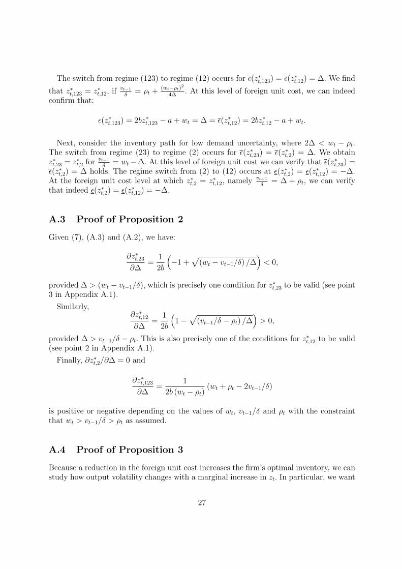
The switch from regime (123) to regime (12) occurs for ε(z∗t,123) = ε(z∗t,12) = ∆. We find
that z∗t,123 = z∗t,12, if vt−1
δ= ρt + (wt−ρt)2
4∆. At this level of foreign unit cost, we can indeed
confirm that:
ε(z∗t,123) = 2bz∗t,123 − a+ wt = ∆ = ε(z∗t,12) = 2bz∗t,12 − a+ wt.
Next, consider the inventory path for low demand uncertainty, where 2∆ < wt − ρt.The switch from regime (23) to regime (2) occurs for ε(z∗t,23) = ε(z∗t,2) = ∆. We obtainz∗t,23 = z∗t,2 for vt−1
δ= wt−∆. At this level of foreign unit cost we can verify that ε(z∗t,23) =
ε(z∗t,2) = ∆ holds. The regime switch from (2) to (12) occurs at ε(z∗t,2) = ε(z∗t,12) = −∆.At the foreign unit cost level at which z∗t,2 = z∗t,12, namely vt−1
δ= ∆ + ρt, we can verify
that indeed ε(z∗t,2) = ε(z∗t,12) = −∆.
A.3 Proof of Proposition 2
Given (7), (A.3) and (A.2), we have:
∂z∗t,23
∂∆=
1
2b
(−1 +
√(wt − vt−1/δ) /∆
)< 0,
provided ∆ > (wt − vt−1/δ), which is precisely one condition for z∗t,23 to be valid (see point3 in Appendix A.1).
Similarly,∂z∗t,12
∂∆=
1
2b
(1−
√(vt−1/δ − ρt) /∆
)> 0,
provided ∆ > vt−1/δ − ρt. This is also precisely one of the conditions for z∗t,12 to be valid(see point 2 in Appendix A.1).
Finally, ∂z∗t,2/∂∆ = 0 and
∂z∗t,123
∂∆=
1
2b (wt − ρt)(wt + ρt − 2vt−1/δ)
is positive or negative depending on the values of wt, vt−1/δ and ρt with the constraintthat wt > vt−1/δ > ρt as assumed.
A.4 Proof of Proposition 3
Because a reduction in the foreign unit cost increases the firm’s optimal inventory, we canstudy how output volatility changes with a marginal increase in zt. In particular, we want
27

to show:
∂Var(q∗t )
∂zt=
< 0 in regime (23)
>< 0 in regime (123)
= 0 in regime (2)
> 0 in regime (12)
.
Consider regime (123). From (2), we have:
∂q∗t (εt)
∂zt=
0 if a+εt−ρt
2b≤ zt,
1 if a+εt−wt
2b< zt <
a+εt−ρt2b
,
0 if a+ε−wt
2b≥ zt.
Since the expected output is
qt,123 =
∫ ε(zt)
−∆
a− ρt + εt2b
dε
2∆+
∫ ε(zt)
ε(zt)
ztdεt2∆
+
∫ ∆
ε(zt)
a− wt + εt2b
dεt2∆
=(2a− (ρt + wt))(2∆− (wt − ρt))
8b∆+zt(wt − ρt)
2∆,
then,∂qt,123
∂zt=wt − ρt
2∆> 0.
It follows that:
∂q∗t (εt)
∂zt− ∂qt,123
∂zt=
−wt−ρt
2∆if a+εt−ρt
2b≤ zt,
1− wt−ρt2∆
if a+εt−wt
2b< zt <
a+εt−ρt2b
,
−wt−ρt2∆
if a+εt−wt
2b≥ zt.
The impact of an decrease in the foreign unit cost on the variance of output is therefore
28

equal to:
∂Var(qt)
∂zt= 2
∫ ∆
−∆
(∂q∗t (εt)
∂zt− ∂qt,123
∂zt
)(q∗t (εt)− qt,123)
dεt2∆
+∂ε(zt)
∂zt(q∗(ε(zt))− qt,123)2 1
2∆− ∂ε(zt)
∂zt(q∗(ε(zt))− qt,123)2 1
2∆
+∂ε(zt)
∂zt(q∗(ε(zt))− qt,123)2 1
2∆− ∂ε(zt)
∂zt(q∗(ε(zt))− qt,123)2 1
2∆
= −2wt − ρt
2∆
∫ ∆
−∆
(q∗t (εt)− qt,123)dεt2∆︸ ︷︷ ︸
=0
+2
∫ ε(zt)
ε(zt)
(q∗t (εt)− qt,123)dεt2∆
=
(wt − ρt
∆
)(zt − qt,123).
Note that the second and the third line are both equal to zero and so is the first term onthe fourth line. Comparing z∗t,123 and qt,123 shows that both zt− qt,123 > 0 and zt− qt,123 < 0are possible.
In particular:
zt−qt,123 =1
8b∆
(2a(wt − ρt)−
(w2t − ρ2
t
)+ 2∆(wt + ρt) + 4bzt(wt − ρt)− 4∆(a− 2bzt
)).
Hence we have:
sign(zt − qt,123) = sign[2a(wt − ρt)−
(w2t − ρ2
t
)+ 4bzt(wt − ρt) + 2∆(wt + ρt)− 4∆(a− 2bzt)
]= sign
[2a(wt − ρt)−
(w2t − ρ2
t
)+ 4bzt(wt − ρt) + 2∆(wt + ρt)− 4∆(a− 2bzt)
]= sign [(wt − ρt − 2∆) [2a− (wt + ρt)] + 4bzt [(wt − ρt) + 2∆]] ,
where the first term is negative due to wt − ρt − 2∆ < 0 and the second term is positive.
Consider now the other three regimes starting with regime (2) where ε(zt) < −∆ <∆ < ε(zt). It is straightforward to find that ∂q∗t (εt)/∂zt = 1 irrespective of εt consistent
with that regime so that qt,2 =∫ ∆
−∆ztdεt/2∆ = zt. It follows that ∂qt,2/∂zt = 1 and
∂q∗t (εt)/∂zt − ∂qt,2/∂zt = 0 so that ∂Var(qt)/∂zt = 0.
The last two regimes have two of the three possible ranges of demand. In the regime(12), valid for −∆ < ε(zt) < ∆ < ε(zt),
∂q∗t (εt)
∂zt=
{0 if εt ≤ ε(zt),
1 if ε(zt) < ε ≤ ∆ < ε(zt).
29

The expected output is:
qt,12 =
∫ ε(zt)
−∆
(a− ρt + εt
2b
)dεt2∆
+
∫ ∆
ε(zt)
ztdεt2∆
=−(a− ρt −∆)2
8b∆+
zt2∆
(a+ ∆− ρt − bzt),
so that∂qt,12
∂zt=
(a+ ∆− ρt − 2bzt)
2∆=
∆− ε(zt)2∆
> 0. (A.4)
Note that ∂qt,12/∂zt < 1 since ε(zt) > −∆. It follows that:
∂q∗t (εt)
∂zt− ∂qt,12
∂zt=
{−∆−ε(zt)
2∆if εt ≤ ε(zt),
1− ∆−ε(zt)2∆
if ε(zt) < εt ≤ ∆ < ε(zt).
The impact of a decrease in the foreign unit cost on the variance of output is thereforeequal to (where we left out the two terms in (∂ε(zt)/∂zt)(q
∗t (ε(zt))− qt,12)2 because they
sum to zero):
∂Var(qt)
∂zt= 2
∫ ∆
−∆
(∂q∗t (εt)
∂zt− ∂qt,12
∂zt
)(q∗t (εt)− qt,12)
dεt2∆
= −2∆− ε(zt)
2∆
∫ ∆
−∆
(q∗t (εt)− qt,12)dεt2∆︸ ︷︷ ︸
=0
+2
∫ ∆
ε(zt)
(zt − qt,12)dεt2∆
=(zt − qt,12)
∆[∆− ε(zt)]
=[∆− ε(zt)]
∆
(zt +
(a− ρt −∆)2
8b∆− zt
2∆(a+ ∆− ρt − bzt)
)=
[∆− ε(zt)]∆
1
8b∆(∆− a+ ρt + 2bzt)
2 > 0.
In the regime (23), valid for ε(zt) < −∆ < ε(zt) < ∆,
∂q∗t (εt)
∂zt=
{1 if −∆ ≤ εt ≤ ε(zt),
0 if εt > ε(zt).
30

The expected output is:
qt,23 =
∫ ε(zt)
−∆
ztdεt2∆
+
∫ ∆
ε(zt)
(a− wt + εt
2b
)dεt2∆
=(2bzt − a)2 + 4bzt(wt + ∆) + (∆− wt)(2a− wt + ∆)
8b∆,
so that:∂qt,23
∂zt=
(2bzt − a+ wt + ∆)
2∆=ε(zt) + ∆
2∆> 0. (A.5)
Note that ∂qt,23/∂zt < 1 since ε(zt) < ∆. It follows that:
∂q∗t (εt)
∂zt− ∂qt,23
∂zt=
{1− ε(zt)+∆
2∆if −∆ ≤ εt ≤ ε(zt),
− ε(zt)+∆2∆
if εt > ε(zt).
The impact of a decrease in the foreign unit cost on the variance of output is therefore
equal to (where we left out the two terms in ∂ε(zt)∂zt
(q∗t (ε(zt))− qt,23)2 because they sum to
zero):
∂Var(qt)
∂zt= 2
∫ ∆
−∆
(∂q∗t (εt)
∂zt− ∂qt,23
∂zt
)(q∗t (εt)− qt,23)
dεt2∆
= −2ε(zt) + ∆
2∆
∫ ∆
−∆
(q∗t (εt)− qt,23)dεt2∆︸ ︷︷ ︸
=0
+2
∫ ε(zt)
−∆
(zt − qt,23)dεt2∆
=[ε(zt) + ∆]
∆
[zt −
(2bzt − a)2 + 4bzt(wt + ∆) + (∆− wt)(2a− wt + ∆)
8b∆
]= − [ε(zt) + ∆]
8b∆2(a− wt + ∆− 2bzt)
2 < 0.
A.5 Endogenous ρ
Suppose that ρt is endogenously determined by the condition ρt = δE(MRt+1). We wantto show that, for all feasible z∗t , a reduction in the foreign unit cost raises z∗t , even if ρt isendogenous. The potential problem to look out for is that a change in vt−1/δ may affectz∗t not only directly but also indirectly through ρt. This is the case, if the expectation offuture foreign unit costs enters E(MRt+1). We also check that the endogenous value of ρtis consistent with the assumptions of the model.
We start with the two feasible z∗t for which the foreign unit cost does not enter
31
E(MRt+1), namely z∗t,2 and z∗t,23. Since both are independent of ρt, there is no indirect ef-fect of vt−1/δ on either z∗2,t or z∗t,23. Evaluating E(MR(z∗t,2)) leads to E(MR(z∗t,2)) = vt−1/δand likewise E(MR(z∗t,23)) = vt−1/δ. Hence ρt = δE(MR(z∗t+1,2)), respectively ρt =δE(MR(z∗t+1,23)), implies ρt = vt, where vt is the expected foreign unit cost of purchasesordered in period t (and used in period t + 1). Since vt−1/δ > ρt, then vt−1 > δρt = δvtwhich holds for any vt−1 ≥ vt since δ < 1.
Consider regime (12). Like above, ρt = δE(MR(z∗t+1,12)) implies ρt = vt. A reductionin the foreign unit cost now has two effects on z∗t,12, namely a direct effect of raisingz∗t,12 whenever vt−1 decreases, and a further indirect effect going in the same direction bylowering ρt through a lower future expected price vt.
In regime (123), like in regime (12), a reduction in the foreign unit cost has both adirect and an indirect effect on z∗t,123. Using ρt = vt to evaluate the combination of thesetwo effects, we obtain
Sign
(dz∗t,123
dρt
)= −Sign{4wt∆(1− δ) + δ(wt − ρt)2} < 0.
Hence a reduction in the foreign unit cost unambiguously raises z∗t,123.
References
[1] Aizenman, Joshua, 2004. Endogenous Pricing to Market and Financing Costs, Jour-nal of Monetary Economics 51(4), 691-712.
[2] Alessandria, George, Joseph P. Kaboski and Virgiliu Midrigan, 2010a. Inventories,Lumpy Trade and Large Devaluations, American Economic Review 100(5), 2304-39.
[3] Alessandria, George, Joseph P. Kaboski and Virgiliu Midrigan, 2010b. The GreatTrade Collapse of 2008-09: An Inventory Adjustment? IMF Economic Review 58(2),254-94.
[4] Benz, Sebastian, Wilhelm Kohler and Erdal Yalcin, 2016. Offshoring and Volatilityof Demand. CESifo Working Paper 5970.
[5] Boute, Robert and Jan Van Mieghem, 2015. Global Dual Sourcing and Order Smooth-ing: The Impact of Capacity and Lead Times, Management Science 61(9), 2080-99.
[6] Bown, Chad, 2013. How different are safeguards from antidumping? Evidence for UStrade policies toward steel, Review of Industrial Organization 42(4), 449-81
[7] Buch, Claudia M., Jorg Dopke and Harald Strotmann, 2009. Does Export OpennessIncrease Firm-level Volatility? World Economy 32(4), 531–551.
32
[8] Di Giovanni Julian and Andrei Levchenko, 2009. Trade Openness and Volatility,”Review of Economics and Statistics 91(3), 558-585.
[9] Evans, Carolyn and James Harrigan, 2005. Distance, Time, and Specialization: LeanRetailing in General Equilibrium, American Economic Review 95(1), 292-313.
[10] Hall, George and John Rust, 2000. An empirical model of inventory investment bydurable commodity intermediaries, Carnegie-Rochester Conference Series on PublicPolicy 52, 171-214.
[11] Hufbauer, Gary Clyde and Ben Goodrich, 2003. Steel Policy: The Good, the Bad andthe Ugly, International Economics Policy Briefs, Number PB03-1, January, Institutefor International Economics, Washington D.C.
[12] Hummels, David and Georg Schaur, 2013. Time as a Trade Barrier, American Eco-nomic Review 103(7), 2935-59.
[13] Hummels, David and Georg Schaur, 2010. Hedging Price Volatility Using Fast Trans-port, Journal of International Economics 82, 15-25.
[14] Kurz, Christopher, Mine Z. Senses and Andrei Zlate, 2017. All Shook Up: Interna-tional Trade and Firm-Level Volatility, mimeo.
[15] Kurz, Christopher and Mine Z. Senses, 2016. Importing, Exporting, and Firm-LevelEmployment Volatility, Journal of International Economics 98, 160-75.
[16] Newbery, David M.G. and Joseph E. Stiglitz, 1984. Pareto Inferior Trade, Review ofEconomic Studies 51, 1-12.
[17] Novy, Dennis and Alan Taylor, 2014. Trade and Uncertainty, NBER Working Paper19941.
[18] Read, Robert, 2005. The political economy of trade protection: the determinantsand welfare impact of the 2002 US emergency steel safeguard measures, The WorldEconomy 28(8), 1119-37.
[19] Sundaram, Asha, 2018. Trade Liberalization and Volatility: Evidence from IndianFirms, University of Auckland, mimeo.
[20] Vannoorenberghe, Gonzague, 2012. Firm-Level Volatility and Exports, Journal ofInternational Economics 86, 57-67.
33