Modeling Conjunctive Water Use as a Reciprocal Externality

R. Garth Taylor, Robert D. Schmidt, Leroy Stodick, and Bryce A. Contor

Corresponding author: Taylor, Department of Agricultural Economics, University of Idaho. Moscow ID 83843 gtaylor@uidaho.edu 208-885-7533. Stodick, Contor, and Schmidt; Idaho Water Resources Research Institute, University of Idaho.

Technical and financial support provided by the US Bureau of Reclamation Pacific Northwest Regional Office, Snake River Area Office, and Science and Technology Program. Funding for Taylor was provided, in part, by the Idaho Agricultural Experiment Station and the USDA-NIFA.

2

Modeling Conjunctive Water Use as a Reciprocal Externality

Conjunctive hydrology gives rise to reciprocal externalities between hydraulically connected

ground and surface water. A partial equilibrium model was formulated for an n-node

groundwater surface water conjunctive use in which economic equilibrium was defined by a

system of complementary slackness equations. Using Mixed Complementary Programming, a

three node example was parameterized using site specific data and functional forms applied to

the general model. This example was solved for equilibrium water prices and quantities in the

respective surface and ground water markets. The model provided a functional framework for

cost/benefit analysis of three policy scenarios in the presence of reciprocal conjunctive use

externalities: (1) Pigouvian tax/subsidy, (2) elimination of the externality through conservation

infrastructure, and (3) aquifer recharge. The Pigouvian policy yielded the highest social welfare

followed by the payment for aquifer recharge. Conservation that eliminated the externality

decreased social welfare.

Key words: conjunctive use, reciprocal externalities, complementary slackness conditions, partial

equilibrium, cost benefit analysis, water conservation, Pigouvian tax, Pigouvian subsidy, water

policy, aquifer recharge.

JEL codes: C61, Q25, Q28, H23

3

Introduction

Exploding municipal, energy, agricultural and environmental water demands are

colliding with limited or diminishing supplies. Policies and projects that would increase water

supplies through cost prohibitive or environmentally unacceptable new infrastructure are being

replaced by those that would reduce demand and/or redistribute supplies. Agriculture, being the

least valued and largest water user (over 80% of water diversions in the West, Hutson et. al

2004) is the principal target of the imperative to allocate and use water more efficiently.

The conventional water planning approaches of supply or demand management fail to

adequately evaluate efficient water project or allocation. Supply management first forecasts a

perfectly inelastic water requirement then calculates the prices to recover costs (Howitt and

Lund, 1999). Demand management ignores water supply elasticity and focuses on reducing

water demand through regulation, conservation, or infrastructure. In rejecting the elasticity of the

opposing supply or demand blade of Marshall’s scissors, both approaches disregard the value of

water. Furthermore, conventional analyses are too often conducted piece-meal, for a specific

water project, irrigation district or municipality, detached from the basin-wide hydrology and

regional economic structure.

From a hydrologic perspective, groundwater and surface water form an integrated

hydrologic system. To manage surface and subsurface water resources efficiently requires

conjunctive water accounting and modeling tools capable of simulating the interactions between

surface water storage or conveyances (rivers, canals, and drains) and groundwater recharge from

those sources. Aquifers created or sustained by irrigation activities extend over vast areas in

every western state. In the aquifers of California’s Central Valley, virtually all recharge is from

“infiltration of irrigation water” (Alley et al. 2002). Aquifers in Idaho’s Eastern Snake River

Plain (Cosgrove, Contor, and Johnson, 2006), and Lower Boise Valley, Nebraska’s North Platte,

Colorado’s South Platte (Howe, 2002) and Washington’s Columbia River Basin, are also

sustained largely by seepage from canals, off-stream reservoirs, or on-farm infiltration. Shakir et

al. (2011) raised alarm concerning the impact of canal water shortages on the conjunctive

groundwater in the Punjab. Schmidt et al. (2013) estimated that about 45% of Boise Project

diversions in the Lower Boise River Basin are consumptively used by canal irrigated crops, with

the remainder either recharging the shallow aquifer or discharging to drains.

4

Externalities occur when the economic activities of one entity affect those of another and

pecuniary remuneration is wanting (Mishan 1971; Baumol and Oates, 1988). Meade (1952)

illustrated a positive reciprocal production externality using the classic example of bees

providing nectar for honey and pollination for apples. In contrast to Meade’s positive/positive

reciprocal externality, conjunctive (joined or connected) surface water and groundwater use is

capable of producing a positive/negative reciprocal externality. Groundwater pumpers near a

canal enjoy a positive externality of canal seepage while inflicting a negative externality of

pumping-induced seepage upon the canal user. The wells which extract tepid water from these

hydrologically connected canals have been aptly labeled “warm water wells” (Strauch 2009).

Water management decisions are often made without regard to exiting surface/subsurface

hydrologic connections or the benefits/costs to other water users in the basin (Booker et al.,

2012; Evans, 2010). In many Western states, groundwater and surface water conjunctive

property rights are poorly defined or non-existent and lack compensation mechanisms to sustain

or curtail conjunctive use, which promulgates externalities (e.g. Strawn, 2004; Evans 2010;

Blomquist et. al. 2001). The resulting conjunctive use externalities cause a divergence between

private and social benefit/cost, with price/market institutions failing to sustain desirable activities

or curtail undesirable activities (Bator, 1958). Omission of conjunctive use externalities also

compromises basin-wide cost/benefit analysis (CBA) as required for Federal water project

planning (U.S. Water Resources Council 1983; Council on Environmental Quality 2009).

The overarching objective of our study is to demonstrate a generalized coupled

hydrologic and economic modeling methodology for conducting basin-wide CBA that

recognizes conjunctive use externalities. The tasks to achieve that goal are threefold: (1)

demonstrate a functional model of conjunctive surface and ground water hydrologic interactions

as conjunctive use externalities, (2) formulate a spatial partial equilibrium model in which

economic equilibrium is defined by a system of complementary slackness equations, and (3)

perform cost/benefit analysis (CBA) of alternative water policies aimed at addressing the market

failures and inefficient water use resulting from conjunctive use externalities.

Methods

5

Within the taxonomy of hydro-economic models, conjunctive use of surface water and

groundwater is a distinct category of research (Harou et al. 2009). Burt’s (1964) foundational

research treated conjunctive groundwater and surface water use as substitutes in an inventory

problem with uncertain supply and controlled demand. The linear programming methods of

optimal recharge and conjunctive groundwater and surface water use (Milligan and Clyde 1970;

O’Mara and Duloy 1984) have been eclipsed by optimal control methods. Noel et al. (1980) used

an optimal control model to determine tax on pumping for the socially optimal spatial and

temporal allocation of groundwater and surface water. Tsur (1990, 1991), and Tsur and Graham-

Tomasi (1991) extended Burt’s optimal control framework with uncertain surface water supplies.

Azaiez (2002) developed a multi-staged decision model to optimize conjunctive use of

groundwater and surface water with artificial recharge. Burness and Martin (1988) determined an

efficient pumping rate to recharge a tributary aquifer to a steady-state aquifer condition from a

perennially losing and hydraulically connected stream. Pongkijvorasin and Roumasset (2007)

expanded upon the static framework of Chakravorty and Umetsu (2005) with an optimal control

model of canal water use and groundwater extraction. Groundwater users were recipients of two

positive externalities, canal conveyance loss and on-farm return flows to the aquifer. In

summary, conjunctive use research has largely focused on the optimal groundwater and surface

water use and optimal aquifer recharge. Despite the explicit label of conjunctive use as an

externality, the hydrologic connection has not been treated as an externality created by

interrelated supply functions.

Two approaches have been taken to the integration of hydrologic with economic models;

network simulation and optimization (Harou et al. 2009). Beginning with Maass et al. (1962),

hydrologic systems have been modeled as networks of water storage, with demand and supply

nodes linked by the conveyance structures of rivers, canals, and pipelines. The network

simulation approach conjoins a hydrologic network model e.g. a river-reservoir prior

appropriations water allocation model (MODSIM, Labadie et. al 1994) with a system-wide

agricultural optimization model (Hamilton et al., 1999 and Houck et al. 2008). While network

simulation models have the necessary basin spatial dimension, these models are limited to

addressing “what if” questions and cannot maximize social welfare, necessary to address

market failures of conjunctive use externalities and conduct CBA of water projects and policies.

6

The partial equilibrium optimization model was introduced in the water literature by

Flinn and Guise (1970), who adopted the concept of interregional trade modeling as developed

by Takayama and Judge (1964). Howe and Easter (1971) used the trading model concept to

evaluate large-scale inter-basin water transfers. Cummings (1974) introduced water benefit and

supply cost functions within a linear programming context representing nonlinear benefit

measures by piecewise linearization. Vaux and Howitt (1984) formulated the first regional

water-trading model linking water demand and supply sectors to demonstrate the cost-

effectiveness of reallocation of water from existing uses as opposed to development of new

supplies. Booker and Young (1994) elaborated upon the water-trading framework, to contrast

benefits of intrastate versus interstate water transfers with salinity and hydroelectric demand also

determining the benefits of water transfers. Further extensions used sequential and dynamic

aspects to analyze and climate or drought on interregional water allocation (Booker, 1995;

Booker and Ward, 1999).

Partial Equilibrium Model

Following Takayama and Judge (1964), partial equilibrium models have been cast as an

optimization problem, where a quasi-welfare or net social function is maximized subject to

constraints, and equilibrium is assumed to be the optimal point that maximizes this objective

function. When Takayama and Judge published their book in the early 1970’s (Takayama and

Judge, 1971) numerical optimization techniques were well understood but mixed complementary

programming (MCP) was in its infancy. With the advent of GAMS (Brooke et al., 1988) and

accompanying solvers, the equilibrium equations can be formulated as complementary slackness

equations in a mixed complementary problem and solved directly. The alternative is to formulate

an objective function optimization problem and assume that the Karush-Kuhn-Tucker (KKT)

conditions coincide with the equilibrium conditions (see Kjeldsen 2000).

The relationship between non-linear optimization used by Takayama and Judge and the

MCP approach is demonstrated by the KKT theorem. Given a function, : n nF R R , the

nonlinear complementary problem (NCP) finds nz R such that 0z , ( ) 0F z , and

0i iz F i where iz is termed complementary to iF . These conditions are written as,

0 ( ) 0z F z and equations of this form, where the operand denotes complementary

7

slackness, are termed complementary slackness equations (Ferris and Munson, 1999). The KKT

theorem demonstrates that a constrained optimization problem, in certain circumstances, can be

transformed into a nonlinear complementary problem. The KKT conditions (a set of

complementary slackness equations) are the first order NCP conditions for the constrained

optimization problem which can be solved using MCP. The Takayama and Judge restriction of

equilibrium using linear supply and demand functions can be generalized to convex function.

A partial equilibrium model is defined for a single commodity (or set of substitutable

commodities) exchanged between nodes where I = set of supply nodes, J = set of demand nodes

and IJ I J = set of allowable arcs between nodes. A supplier produces a commodity at node

i and ships a quantity ,i jX to node j along arc ,i j . A supplier at node i can ship to the same

node i, thus I J is not necessarily empty. The exogenous variables are the demand functions

( )jP q j J , supply or marginal cost functions ( )iP q i I and transportation cost function

, ( , )i jt i j IJ . The endogenous variables are: jq = quantities demanded j J , iq = quantities

supplied i I , ,i jX = quantities shipped from node i to node j ( , )i j IJ , j = market

demand price j J and i = market supply price i I . Per the notation of Takayama and

Judge, a variable superscript is a node index, not an exponent.

Absent non-convexities and assuming the equations have a unique solution; five sets of

equations define economic equilibrium (Takayama and Judge, definition 2.4.9).

(1a) ( )i i i iq P q i J

(2a) ( )i i i iq P q i I

(3a) , , ,ii j i j jx t i j IJ

(4a) ,i j i i

i

x q i J

(5a) ,i i

i jj

q x i I

where the overscore operand indicates the equilibrium value and the operand denotes

complementary slackness. Thus, ( )x f y means 0x , ( ) 0f y and ( ) 0x f y . Equations 1a

state that, at equilibrium, if the quantity demanded is greater than zero, demand price must equal

marginal benefit. Equations 2a state that, at equilibrium, if the quantity supplied is greater than

8

zero, supply price must equal marginal cost. Together, equations 1a and 2a ensure the existence

of a Pareto optimum at equilibrium. If the quantity traded is greater than zero, Equation 3a

ensures locational price equilibrium, by equating the sum of supply price and transportation cost

with demand price. Equations 4a state that, at equilibrium, if the demand price is greater than

zero, quantity demanded must equal the sum of all shipments to that node from all supply nodes.

Equations 5a state that, at equilibrium, if the supply price is greater than zero, all shipments from

a supply node must equal the total quantity produced at that node. Equations 4a and 5a ensure

market quantity equilibrium.

Partial Equilibrium with Conjunctive Use Externalities

The conjunctive hydrologic connection creates a Meade production externality where

supply functions of groundwater and canal water users become interrelated. The conjunctive use

externality is one-way or reciprocal depending on the surface water and groundwater connection,

and positive (e.g. aquifer recharge) or negative (e.g. reduced canal flows) depending on the

recipient’s production function. When a leaky canal is not hydraulically connected to the aquifer,

the canal water user gifts the groundwater pumper with a one-way positive externality of passive

seepage (i.e. independent of pumping). The canal user’s water demand is thus an argument in the

supply function of the groundwater pumper but the pumper’s demand is not an argument in the

canal supply function. When a leaky canal is hydraulically connected to the aquifer and a

hydraulic gradient exists as a result of pumping, the groundwater pumper reciprocates by

inflicting a negative externality of pumping-induced seepage on the canal user. With a reciprocal

externality, passive and pumping-induced canal seepage enter into the supply function of the

groundwater pumper as a positive externality, and the pumper inflicts a negative externality of

induced seepage upon the canal water user as an additional transportation cost. Production

externalities necessitate the specification of interrelated supply equations of the equilibrium

conditions 2a, 3a, and 4a of the basic model. Equations 1a and 5a, which do not contain supply

expressions, are thus unchanged from the basic model. In contrast to 2a, where price equals only

pecuniary marginal costs ( ( ))i iP q , at equilibrium price equals pecuniary and externality

marginal cost ,( ( ,{ })k ki jP q X :

9

(2b) ,( ,{ })k k k ki jq P q X k I

With the reciprocal externality, the locational price equilibrium equations (3a) must account for

the marginal cost of seepage in equating supply price at node i with the demand price at node j

(i.e. the marginal cost of seepage at the head of the canal with demand price at the end of the

canal , , , , { }, ,

{ }

( ) ii j i j i j j i j k i j

k

X t X X S . The transportation cost is the seepage along the arc of a

leaky canal: { }, , ,( ,{ })kk i j i jS X q where ,i jX is the diversion at the head of the canal and { }kq k I

is the total pumping rate of pumpers that induce canal seepage. Taking the derivative of both

sides of the equation with respect to ,i jX results in the price linkage equation;

{ }, ,,

{ } ,

0k i jii j j j

k i j

St

X

, so that 3a becomes:

(3b) ,{ }, ,

,

( ,{ }), ,

{ }

,

ki jk i j

i j

S X qii j i j j j X

k

X t i j IJ

Equation 3b thus states, that at equilibrium, if the quantity traded is greater than zero, the sum of

supply price and transportation cost (i.e. seepage cost) must equal demand price. If the demand

price at node j is greater than 0, then at equilibrium, the quantity demanded must equal total

quantity transported less seepage: , { }, , ,{ }

( ,{ })kj i k j i j i i

j j k

X S X q q i J . With the reciprocal

externality, the excess demand for canal water is eliminated by:

(4b) , { }, , ,{ }

( ,{ })ki j i k j i j i i

i j k

X S X q q i J

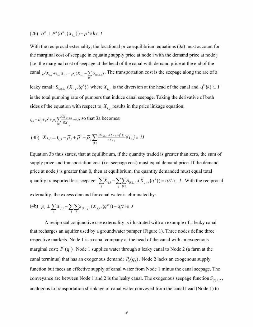
A reciprocal conjunctive use externality is illustrated with an example of a leaky canal

that recharges an aquifer used by a groundwater pumper (Figure 1). Three nodes define three

respective markets. Node 1 is a canal company at the head of the canal with an exogenous

marginal cost; 1 1( )P q . Node 1 supplies water through a leaky canal to Node 2 (a farm at the

canal terminus) that has an exogenous demand; 2 2( )P q . Node 2 lacks an exogenous supply

function but faces an effective supply of canal water from Node 1 minus the canal seepage. The

conveyance arc between Node 1 and 2 is the leaky canal. The exogenous seepage function {3},1,2S ,

analogous to transportation shrinkage of canal water conveyed from the canal head (Node 1) to

10

canal end (Node 2), determines recharge of the aquifer used by Node 3. The farm at Node 3 is

supplied by an aquifer that is in part recharged by canal seepage and has a demand for pumped

water; 3 3( )P q . Node2 sole water source is the canal. Node 3 water source is seepage from the

canal (both passive and induced) and aquifer recharge from sources other than the canal. The

marginal cost function for groundwater at Node 3 equals the pecuniary marginal costs 3 3( ( ))P q

and the externality of seepage gifted by Node 2, {3},1,2S . The indices for the example are thus;

{1,3}, {2,3} {(1,2), (3,3)}i j and ij .

Economic equilibrium is defined by the system of complementary slackness equations

(2b, 3b and 4b). The endogenous equilibrium prices 1 2 3, , and and quantities 1 2 3, , q q and q

, can be determined by solving the complementary slackness equations using MCP or by

maximizing a social welfare objective function (e.g. Booker and Young 1994; Booker and Ward,

1999). In our example, complementary slackness conditions were programmed in GAMS and

solved using the PATH solver (Ferris and Munson 1999). Equilibrium prices and quantities are

then limits on the respective consumer and producer surplus integrals.

Exogenous Functions

The two exogenous demand functions (Node 2 demand at the end of the canal and Node

3 demand at the well head); two exogenous marginal cost functions (Node 1 supply at the head

of the canal and Node 3 supply of groundwater at the well head), and an exogenous

transportation cost of canal seepage are outlined below and detailed with data in the Appendix.

Typically, hydro-economic models represent hydrology through constraints (Booker et

al., 2012). In contrast, the conjunctive hydrologic connection of the seepage function is an

argument in both the groundwater and canal water supply functions and thus the seepage

function defines the reciprocal externality. The aquifer, from which Node 3 pumps, is recharged

by two sources, canal seepage and so-called far-field sources at the boundaries of the hydrologic

model. Seepage is a convex function of the amount of water conveyed in the canal from Node 1

to Node 2 (X(12)) and the amount of pumping by Node 3 (q3 ):

31 1,2 3

{3},1,2 0 2 1,21 1a X a qS a e a X e

.

11

Total seepage ( {3},1,2S ) is the sum of: (1) passive seepage (the first-term), a function only of

canal diversion (X(1,2)), (a0 is the maximum canal seepage possible), and (2) induced seepage (the

second term), a function of canal diversion (X(12)) and pumping (q3). Marginal seepage with

respect to canal diversion is:

(1,2)

{3},1,2

1,2

0X

SMS

X

and

2{3},1,2

21,2

0S

X

.

(1,2)XMS is thus downward sloping. As more water is diverted into the canal seepage increases

and the water table beneath the canal rises. As the water table connects with the canal over an

increasing length of canal, the head gradient between the canal and aquifer is reduced, so that as

1,2X increases (1,2)XMS decreases.

Marginal seepage with respect to pumping is:

3

{3},1,2

30

q

SMS

q

and

2{3},1,2

2 30

S

q

.

3qMS is thus downward sloping -- with increased pumping (ceteris paribus the canal head

condition) the water table declines, the aquifer becomes disconnected from the canal (over a

greater length of the canal), and the pumper is less able to induce seepage i.e. as 3 0q

MS

seepage is increasingly passive.

The locational price equilibrium (Eqn. 3a) is determined by equating the sum of supply

price and transportation cost (effective supply) with demand price. Effective cost of supply at

Node 2 ( 2P ) is the cost of water supplied at the head of the canal plus the marginal cost of

seepage; 1,2

2 12 XP P MS where the exogenous marginal cost for Node 1 at the head of the

canal (in our example, 11P k ) and 2 is the price at Node 2. In our example, the total charge at

the head of the canal equals k1X1 where k1 is a fixed O&M charge, thus 11P k . P2 is thus the

sum of exogenous levy at canal head plus the externality of 1,2XMS which is determined in part

by the amount of pumping (q3) of Node 3. The quantity of water delivered to Node 2 at the end

of the canal is the quantity at the head of the canal net of canal seepage. Downward sloping

12

seepage costs are added to a fixed levy resulting in an effective supply cost at Node 2 which

declines as diversion increases.

The marginal cost of groundwater to Node 3 at the well head is: 32 3 ;P k k lift where k2

is a fixed pumping cost, k3 is the power cost per foot of pumping lift, and pumping lift is;3

1 2 1,2( )0

b q b Xlift b e . P3 is thus a function of the exogenous pumping cost parameters plus the

canal seepage externality, as determined by the actions of Node 2. As pumping increases, the

water table drops and become disconnected from the canal, thus 3 0q

MS and seepage becomes

increasingly passive. Simultaneously, the drop in water table causes the marginal cost of

pumping to escalate.

The two exogenous irrigation demand functions correspond spatially to the respective

supply functions, the well head and head gate at the end of the canal for Nodes 3 and 2,

respectively. Demand is short-run, exhibiting decreasing marginal returns to the variable input of

water and with crop mix, acreage, and irrigation technology fixed. The general functional of the

demand is; 30 1(1 )i iP q , where β0, β1, and β2 and is parameterized using case specific

agronomic data on crop yield, evapotranspiration, irrigation application, and irrigation efficiency,

and commodity prices (see appendix, Contor et al., 2008).

ResultsandAnalysis Externalities result in undesirable market behavior when market institutions fail to sustain

desirable activities or reduce undesirable activities (Bator, 1958). A Pigouvian wedge thus arises

between private and social cost/benefit, with positive externalities under produced and negative

externalities over produced. The reciprocal conjunctive use externalities result in failures in the

surface water and groundwater markets; the positive externality of passive seepage is under

produced and the negative externality of induced seepage is over produced.

Using the above three node example, three scenarios were developed to illustrate the

application of partial equilibrium modeling with conjunctive use externalities. The first scenario

is a Pigouvian tax/subsidy internalization of the reciprocal externalities. The two subsequent

scenarios are common management alternatives intended to mitigate conjunctive use

13

externalities; (1) eliminating the externality with water conservation infrastructure and (2)

augmenting the externality with managed aquifer recharge. Equilibrium prices, quantities and

surpluses for each scenario are reported in Table 1. The Pigouvian tax/subsidy and aquifer

recharge scenario results are displayed in Figure 2a and 2b and Figures 3a and 3b, respectively.

The figures illustrated three points: (1) the production externality of conjunctive use shifts only

supply the functions, (2) the CBA that is performed numerically and can be illustrated

graphically (Griffin 1998) and (3) the tax/subsidy that eliminates the wedge between the private

and social causes a feedback in the reciprocal groundwater or canal water market.

Baseline

The baseline is the “without” scenario in the with-versus-without evaluation required by

CBA. In the baseline, the leaky canal is connected to the aquifer. The groundwater pumper

receives a positive externality of reduced pumping lift from canal seepage and pumping inflicts a

negative externality upon canal user by inducing additional seepage. Evident in the equilibrium

prices and quantities is the rudimentary water budget for the baseline. In the canal water market,

Node 1 supplies 3,097AF priced at $15/AF of which 2,130AF reaches Node 2 who is willing-to-

pay $21.65/AF for the water delivered at the canal end. Node 2 makes a payment to Node 1 in

the amount of $46,406 $15 3097 which includes $14,505 $15 3097 2130 for water

not received, i.e. canal seepage. In the groundwater market, Node 3 pumps 1,283AF (286AF of

induce seepage plus 681AF of passive seepage plus 316AF from sources other than seepage) (see

endnote 1) for which he pays $30.65/AF in pumping costs. The Node 3 pumper thus makes a

payment to the Node 3 supplier (i.e. the power company) in the amount of $39,325

$30.65 1, 283AF . Baseline surplus totals to $164,087; $90,900 Node 2 consumer surplus,

$64,242 Node 3 consumer surplus and $8,946 Node 3 producer surplus. The horizontal supply

function of Node 1 yields no producer surplus.

Pigouvian Tax/Subsidy

In a competitive equilibrium, the welfare of two agents depends only on consequences of

their own choices. An externality creates an asymmetry between social and private prices.

14

Internalization forces both agents to account for the consequences of their actions on the other’s

welfare by aligning prices. Absent internalization (i.e. the base case), the canal water user

responds only to the pecuniary supply cost of the canal company and the shrinkage cost of

seepage. Ignored is the reduction in costs that the pumper receives from canal seepage. Similarly,

the pumper is signaled only by the pecuniary cost of pumping, ignoring the cost to the canal

diverter of pumping-induced seepage. A Pigouvian tax/subsidy internalizes the externality, by

aligning marginal supply prices of canal diverters and groundwater pumpers. The price

alignment signals to decrease production of the negative externality (pumping induced seepage)

and increase production of the positive externality (canal diversions that create seepage).

To internalize the reciprocal conjunctive use externality, the canal water supply function

is redefined as the pecuniary marginal cost at Node 1 plus the negative externality of seepage in

the transportation of water from Node 1 to Node 2 plus a Pigouvian subsidy. The subsidy equals

the reduction in marginal cost that canal seepage provides the Node 3 groundwater pumper. To

determine the subsidy, the price linkage equation (3b) which equates canal water demand prices

with the sum of supply prices (including seepage and transportation costs) is replaced with

equation 3c:

(3c) { }, , ,

,

( ,{ })

, , ,k

k i j i j

i j

S x qii j i j j j xx t i j IJ

,

where,

3

1,2

3 31,2

1,2 0

( ,{ })q

XMC P q X dqX

is the Pigouvian subsidy to the canal diverter, defined

as the Node 3 marginal cost of pumping with respect to canal diversion. Equation 3c states, that

at equilibrium, if the quantity of water diverted in the canal is greater than zero, the sum of

supply price, and seepage cost plus the Pigouvian subsidy equals the demand price.

Similarly, the groundwater supply function is redefined as the pecuniary cost of pumping

at Node 3 plus the marginal cost of pumping induced canal seepage to the canal diverter at Node

2. To determine the tax, the price linkage equation (2b) which equates groundwater demand price

with supply price is replaced with equation 2c:

(2c) ,( ,{ })k k k ki jq P q X k I

15

where 32 qMS is the Pigouvian tax imposed on the groundwater pumper, defined as the

marginal cost to Node 2 of pumping induced seepage. Equation 2c states that at equilibrium, if

the quantity of groundwater pumped is greater than zero, the pumping cost plus the Pigouvian

tax equals the demand price. Together, α and monetize or price canal seepage in both the

surface water market and the groundwater market, and equations 2c and 3c ensure the existence

of a social optimum at equilibrium.

The Pigouvian tax/subsidy aligns prices to erase the wedge between social and private

costs in surface water and groundwater markets that arise from the canal seepage externalities.

However the reciprocal nature of the externalities means that the tax/subsidy accounts for only a

portion of the total wedge between social and private supply cost. A portion of the wedge in each

market is erased through feedback from the other market. The imposition of an optimal tax on

Node 3 pumping and an optimal subsidy for Node 2 canal diversion nevertheless insures that the

marginal benefit of canal seepage to groundwater pumpers matches the marginal cost of seepage

to the canal diverter.

In the surface water market, the Pigouvian subsidy shifts the supply function downward

from the baseline (Figure 2a). At equilibrium, Node 1 supplies 3,692AF to Node 2 (an increase

of 595AF over the base case) for which Node 2 is willing-to-pay $8.31/AF. The Pigouvian

subsidy (β) for canal diversion is $9.23/AF. Node 2 pays Node 1 $55,383 ($15*3,692) which

includes seepage costs of $17,250 (1,150*$15). Assuming the base case canal diverter supply

function without the subsidy, but the scenario 2 rate of diversion and pumping, the equilibrium

price at Node 2 is $21.61/AF (Figure 2a) (see endnote 2). The total wedge between social and

private cost in the surface water market is therefore $13.30 ($21.61 - $8.31). Of this, $9.23 is

erased by the canal diversion subsidy (A to B in Figure 1a) and $4.07 is erased by feedback from

the groundwater market (B to C in Figure 2a). The feedback is a consequence of the tax on

groundwater pumping which reduces pumping and thereby the induced component of canal

seepage.

In the groundwater market, the Pigouvian tax shifts the supply function upward from the

baseline (Figure 2b). At equilibrium, the Pigouvian tax (α) on pumping is $0.45/AF. However, as

a consequence of the combined tax and subsidy, pumping increases by 23AF (1,306 – 1,283),

and the price of groundwater declines from $30.65/AF to $25.72/AF. Again, assuming the base

16

case groundwater pumper supply function without the tax, but the rate of diversion and pumping,

the wedge between social and private cost in the groundwater market is $5.01 ($30.73-$25.72)

(figure 1b). The $0.45/AF tax, on pumping has the intended effect of reducing induced canal

seepage, although it actually increases the wedge between private and social groundwater supply

(A to B in Figure 2b). The wedge in supply is only erased by the $5.46 feedback from the surface

water market (B to C in Figure 2b) (see endnote 3). The reciprocal externality produces feedback

between the surface and groundwater markets that reinforces or cancels the tax/subsidy effect.

In the groundwater market, the subsidy increases canal diversion which then increases seepage

available for pumping which more than offsets the tax induced reduction in pumping. Despite

taxing the negative externality of pumping, the marginal cost of pumping declines (internalized

supply, Figure 2b) and pumping increases from the private equilibrium (1283) to the social

equilibrium (1306).

Internalization with a tax/subsidy increases the welfare of both groundwater pumper and

canal diverter. In the with-versus-without CBA comparison, total irrigator surplus increased by

21% over baseline. In the groundwater market, consumer surplus increased by 10% ($64,242 to

$70,625), and in the surface water market consumer surplus increases by 34% ($90,900 to

$121,986). The benefit of seepage received by Node 3 outweighs the tax levy and the subsidy

received by Node 2 outweighs the seepage loss. As tax and subsidy, and generate an optimal

social equilibrium, neither can be increased or decreased without being offset by greater social

cost or reduced social benefit. A complete market now exists where trade is unimpeded, thus

ensuring by definition, the gains in efficiency from trade (Randall, 1983). The Pigouvian

incentive requires exogenous cash flows i.e. collected tax revenues are received and subsidy is

funded by an external agent. A tax paid to the injured party (canal user) or a subsidy paid by the

beneficiary (pumper) distorts the tax/subsidy incentive (Baumol and Oates, 1988).

Correcting the market failure by omniscient regulation of the reciprocal externality

requires pumping restrictions and canal diversion increases. Regulation of induced seepage

damage alone (e.g. a binding constrain on pumping) will simply reproduce the equilibrium

quantities and welfare of the baseline scenario. Prior appropriations regulations to protect senior

canal or river rights from the damage of induced seepage are usually enforced as well setbacks or

outright bans. For example, Oregon (Oregon Water Resources Department 2010) mandates a

17

quarter mile set back from the river for wells in a riparian aquifer. Absent damage to the senior

water users, prior appropriations regulation cannot compel canal users to “waste water” for

aquifer recharge (Fereday et. al 2006). Regulation is thus limited to pumping restrictions reduces

the benefit derived from passive seepage intended to prevent the damage of pumping-induced

seepage.

Eliminating the Externality

The externality can be eliminated by lining the leaky canal. Canal lining is promoted as

conservation panacea that maintains agricultural production, while liberating water for

environmental or municipal use (Rodgers 2008; Hanak et al. 2010). Millions have been

expended to subsidize agricultural water conservation by either reducing on-farm infiltration or

improving conveyance efficiency. CBA for water conservation infrastructure are required to

account for the costs and benefits, including those of the current recipients of the seepage

externality.

When the canal is lined the cost of seepage is no longer imposed upon the canal diverter.

The quantity supplied by Node 1 (2,327AF) equals the quantity demanded at Node 2, making

Node 1 supply price ($15) equal to Node 2 demand price. Canal diverter demand increases

196AF (2,327 - 2,130). Absent canal seepage, aquifer levels decline, pumping cost increases

from $30.65 to $95.24/AF and pumping declines by 875AF (1,283-408). Surface water market

consumer surplus increased by 16% ($90,900 to $105,709), offset by a decrease in consumer and

producer surplus in the groundwater market by 64%. Total surplus, the CBA of with-versus-

without comparison, declined 67% ($110,239 to $164,087). In our example, construction costs

are ignored and the sole beneficiary of canal lining is the short run increase in irrigation intensity

of the existing crop mix and acreage of the canal water user.

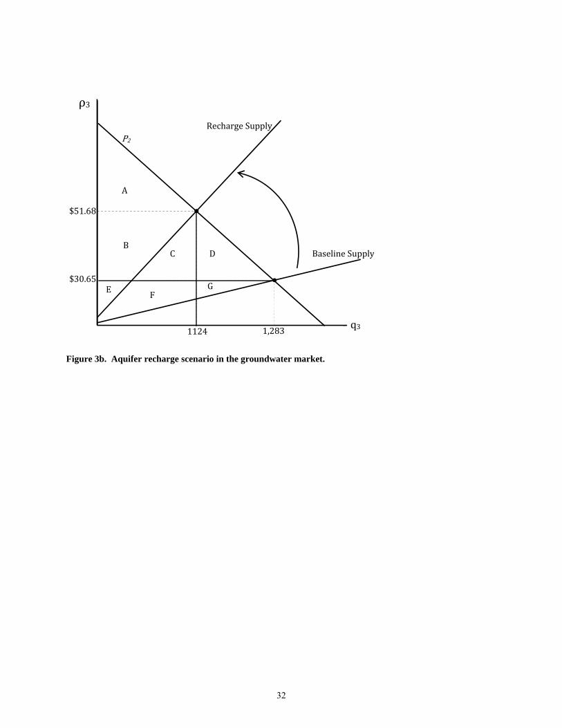
Aquifer Recharge

As illustrated in previous research, aquifer recharge is an accepted policy in conjunctive

use management (Blomquist et al. 2001). In contrast to the external Pigouvian tax/subsidy flows,

aquifer recharge payments are internal -- the junior appropriator pay to receive the benefit or

18

compensate for damages to the senior. As the case with most conjunctive hydrology situations,

the pumper has an adjudicated right that is junior to the canal user whose seepage created the

aquifer. Thus, in our example, the junior pumpers compensate the senior canal users for

increased diversions to recharge the aquifer. Diversions for recharge are assumed to occur during

the irrigation season, rival with canal demand.

Canal diversion is priced via a payment from Node 3 to Node 2 that matches the decrease

in total pumping cost attributable to the seepage resulting from canal diversion. The payment is

calculated by integrating the groundwater pumpers’ marginal cost function with respect to

pumping yields total pumping cost, and differentiating with respect to canal diversion to yield

the marginal cost of pumping with respect to diversion:

3

1,2

3 31,2

1,2 0

( ,{ })q

XMC P q X dqX

. The

total value of canal seepage to groundwater pumpers is1,2

31,2 XX MC , and the payment rate for

canal diversion per acre-foot of groundwater pumping is1,2

1,2 33 X

XMC

q. Groundwater pumpers

maximize their returns by paying the canal diverter this amount for each acre-foot of water

diverted down the canal. In turn, this payment is inserted into the canal water and groundwater

price linkage equations, (3b) and (2b). Equation 3d states, that at equilibrium, if canal diversion

is greater than zero, the sum of supply price, transportation and seepage costs, minus the

payment from groundwater pumpers equals the canal diverter’s marginal demand price.

(3d) { }, , ,

,

( ,{ })

, , ,, 0

( ,{ }) ,

k

kk i j i j

i j

qS x qi k

i j i j j j i jxk i j

x t P q x dq i j IJx

Equations 2d states, that at equilibrium, if the quantity of groundwater pumping is greater than

zero, the marginal cost of pumping plus the seepage payment to canal diverters equals the

groundwater pumper’s marginal demand price.

(2d) ,, ,

, , 0

( ,{ }) ( ,{ })

kqi jk k k k k

i j i jki j i j

Xq P q X P q X dq k I

q X

In the groundwater market, the transfer payment raises the marginal cost of pumping and

thus shifts the supply function upward from the baseline (Figure 3b). The transfer payment from

Node 3 to Node 2 increases Node 3 marginal cost by $21.04/AF ($51.68 - $30.65) relative to the

19

base case scenario. As a consequence, groundwater pumping decreases by 159AF (1,283 - 1124)

relative to the base case.

In the surface water market, the transfer payment lowers the marginal cost of deliveries to

the end of canal and thus shifts the supply function downward from the baseline (Figure 3a). In

the surface water market, the transfer payment reduces Node 2 marginal cost by $11.86 ($21.65-

$9.79) from the base case. As a result, the quantity of water shipped from Node 1 to Node 2

increases by 506AF (3604 - 3097) and Node 2 increases demand by 362AF (2492 - 2130). The

increase in diversion increases seepage by 145AF (1112 - 967). The Node 3 groundwater pumper

pays the Node 2 canal diverter $8.17/AF for canal water diverted at Node 1 which translates into

a payment of $26.21/AF of groundwater pumped. The total payment by Node 3 is $29,447

($26.21 × 1,112) which matches the total receipts of Node 2, $29,447 ($8.17 × 3,604) i.e. the

decrease in total pumping cost attributable to the seepage resulting from canal diversion.

In the surface water market, Node 2 consumer surplus increased by 30% ($90,900 to

$118,253); (A+B+C) – A in figure 3a). In the groundwater market, consumer surplus for Node 3

decreased by 40% ($64,242 to $38,737); (A+B+C+D) – A in figure 3b). Node 3 producer surplus

increases 282%, from $8,946 (E+F+G in figure 3b) to $34,214 (B+E in figure 3b). The big

increase in Node 3 producer surplus is attributable to the payment made to Node 2. The

groundwater pumper is better off paying for relatively cheap electricity than paying the canal

diverter for relatively costly seepage water. The managed recharge alternative lifts net social

welfare above the baseline by 17% ($164,087 to $191,204). Even after making payments for

canal seepage, the groundwater pumpers’ surplus is not exhausted. The surplus of Node 2 canal

diverters damaged by the negative externality of pumping induced seepage increases with receipt

of payment from groundwater pumpers. Although the managed recharge scenario does not

penalize pumping induced seepage, the CBA social benefit from this scenario exceeds that of the

baseline status quo.

In contrast to the Pigouvian tax and subsidy that corrects both sides of the reciprocal

externality, only the positive externality of seepage is addressed by the recharge payment. The

negative externality of induced seepage, addressed by a payment from the canal to the pumper to

curtail pumping, is left uncorrected. The recharge payment addresses the market failure in that

the senior appropriator canal user cannot be compel to “waste water” to sustain the positive

20

externality of seepage to the aquifer (Fereday et al. 2006). The property right establishes that the

pumper needs to pay for passive seepage that he previously received free. While payment is a

potential remedy for the market failure the necessity for property rights contravenes a long

standing principle of prior appropriation; the loss of physical control of water, whether through

surface returns or percolation to aquifers, returns the water to public ownership.

Conclusions

Aquifers created or sustained by surface water are a global phenomenon. Previous

research on conjunctive use failed to treat conjunctive ground and surface water use as an

externality of un-priced and interrelated supply functions. Reciprocal conjunctive use

externalities thus result in failures in both surface and groundwater markets.

Per our goal of functionality, an n-dimension generalized partial equilibrium model of

conjunctive groundwater and surface water use was formulated. Using MCP, a three node

example was parameterized with site-specific data and was solved for equilibrium water prices

and quantities in the respective surface water and groundwater markets. The three exogenous

variables are: (1) demand, for various crops, irrigation technologies and scalable to any acreage,

(2) supply, from pumping costs and canal company levies and (3) the transportation arc, a

seepage function estimated from a groundwater model. Functionality was further demonstrated

in the CBA performed on three conjunctive management policies; tax/subsidy, conservation, and

aquifer recharge. A basin water budget, which accompanies groundwater models, can provide an

external check on baseline scenario results. The partial equilibrium framework and data can be

replicated; calculation of the demands and marginal costs are well documented but seepage

functions deserve further research.

The Pigouvian tax/subsidy aligns private and social price to erase the wedge between

private and social cost and when imposed on a one way externality results in an unambiguous

decrease or increase of that externality. In contrast, the tax/subsidy on a reciprocal externality

produces feedback between the markets that reinforces or cancels the tax/subsidy effect. In our

example, the subsidy increased canal diversion which then increased seepage available for

pumping which more than offsets the tax induced reduction in pumping. Pumping quantity at the

social equilibrium (1306AF) increased over the private equilibrium (1283AF), despite taxing the

21

negative externality of pumping. The feedback effect improves the welfare of the recipient – e.g.

the tax discourages the negative externality of pumping to the benefit of canal and the subsidy

encourages canal diversions to the benefit of the pumper. The magnitude of the feedback is

determined by the relative magnitude and elasticity of exogenous supply, demand and

transportation variables.

Of the three policy scenarios, internalizing the externalities via a tax/subsidy generated

the greatest social benefit. Conservation failed the CBA -- the foregone benefit of canal seepage

to the pumpers by eliminating the externality outweighs the increase in canal benefit. In the

recharge scenario, canal seepage is priced via a payment from pumper to canal water user that

matches the decrease in total pumping cost attributable to the seepage resulting from canal

diversion. In our example, total surplus of the recharge policy was 97% of the Pigouvian

scenario. With the recharge payment, the equilibrium quantities, in all three markets, was only

slightly less than the Pigouvian scenario. However, the price of water at node 3, driven by the

payment, increased from $25.72 to $51.68.

Market failures arise from poorly assigned and/or enforced property rights. Governance

often fails to legally acknowledge conjunctive hydrologic connections, let alone recognized

conjunctive use as a reciprocal externality. The Prior Appropriation Doctrine defines and

protects property rights not correct the externality by maximizing social welfare as does partial

equilibrium framework. The lack of property right extends to both sides of the reciprocal

externality: junior groundwater users are not forced to pay for the seepage that they now freely

enjoy nor are senior canal users compensated for the damage of pumping induced seepage. Prior

appropriation removes the incentive of seepage payments because once the seepage leaves the

canal diverters control, the water reverts to the public domain to be appropriated for beneficial

use. On other side of the reciprocal, the beneficiary of seepage has no mechanism to invite

additional seepage. Absent damage to the senior water users, prior appropriations regulation

cannot compel canal users to “waste water” for aquifer recharge (Fereday et. al 2006).

Cheung’s (1973) rejoinder to Meade’s bee example, pointed out that the market failure of

a reciprocal externality can be corrected, without government intervention, by payments from

apple to bee farmers. Reciprocal conjunctive use externalities have not been similarly resolved

and as water supplies shrink and demands grow, the lawsuit and water calls etc. are symptoms of

22

the proliferation of market failure conflicts. Continued reliance upon regulation of conjunctive

externalities will increase inefficient water use that a water-scare society ill afford. A functional

model of reciprocal conjunctive use externalities is a first step in the investigation of conjunctive

water management policy alternatives.

References

Alley, W.M., R.W. Healy, J.W. LaBaugh, and T. E. Reilly. 2002. Flow and Storage in Groundwater Systems. Science 296: 1985-1190.

Azaiez, M. N. 2002. A model for conjunctive use of ground and surface water with opportunity costs. European Journal of Operational Research 143: 611–624.

Bator, F. 1958. The Anatomy of Market Failure, Quart. J. of Economics 782(3): 351 - 379.

Baumol, W J. and W. E. Oates. 1988. The Theory of Environmental Policy Externalities, Public Outlays, and the Quality of Life. 2nd edition Prentice-Hall New Jersey.

Blomquist, W., T. Heikkila T, and E. Schlager E. 2001. Institutions and Conjunctive Water

Management Among Three Western States. Natural Resources Journal 43(1): 653–683.

Booker, J. F. 1995. Hydrologic and economic impacts of drought under alternative policy responses, Water Res. Bulletin 31(5): 889-907.

Booker, J. F. and F. A. Ward. 1999. Instream Flows and Endangered Species in an International River Basin: The Upper Rio Grande. Amer. J. Ag. Econ. 81(5): 1262-1267.

Booker, J. F., R. E. Howitt, A. M. Michelsen, and R. A. Young. 2012. Economics and the Modeling of Water Resources and Policies. Natural Resource Modeling Journal 25th Anniversary Special Issue, 25(1).

Booker, J. F. and R. A. Young. 1994. Modeling Intrastate and Interstate Markets for Colorado River Water Resources. J. Environ. Econ. and Management. 26 (1): 66-87.

Burness, H. S. and W E. Martin. 1988. Management of a Tributary Aquifer. Water Resources Research 24(8): 1339-1344.

Brooke, A., D. Kendrick, and A. Meeraus.1988. GAMS A User’s Guide. The Scientific Press,

Redwood City, California.

Burt, O. R., 1964. The Economics of Conjunctive Use of Ground and Surface Water. Hilgardia, 36, 31-111.

Chakravorty, U. and C. Umetsu. 2003. Basinwide water management: A spatial model. J. Environ. Econ. Mgt. 45 1-23.

Cheung, S. 1973. The fable of the bees: An economic investigation. Journal of Law and Economics. 16:11-33.

23

Contor B.A., G. Taylor and G. Moore. 2008. Irrigation Demand Calculator: Spreadsheet Tool for Estimating Demand for Irrigation Water, WRRI Technical Report 200803, http://www.iwrri.uidaho.edu/documents/200803-1_revision.pdf?pid=108520&doc=1.

Cosgrove, D.M., B.A. Contor, and G.S. Johnson. 2006. Enhanced Snake Plain Aquifer Model Final Report, Idaho Water Resources Research Institute: http://www.if.uidaho.edu/~johnson/FinalReport_ESPAM1_1.pdf

Council on Environmental Quality. 2009. Proposed National Objectives, Principles and Standards for Water and Related Resources Implementation Studies http://www.whitehouse.gov/sites/default/files/microsites/091203-ceq-revised-principles-guidelines-water-resources.

Cummings, R. G. 1974. Interbasin Water Transfers: A Case Study in Mexico. Johns Hopkins University Press, Baltimore, MD.

Evans, A. 2010. The Groundwater/surface Water Dilemma in Arizona: a Look Back and a Look Ahead Toward Conjunctive Management Reform. Phoenix Law Review 3: 269-291.

Fereday, J., C. H. Meyer, and M. C. Creamer. 2006. Water Law Handbook: The Acquisition, Use, Transfer, Administration, and Management of Water Rights in Idaho. Givens and Pursley, Attorneys at Law, Boise ID.

Ferris, M. and T. Munson. 1999. Complementarity Problems in GAMS and the PATH

Solver.GAMS – The Solver Manuals. GAMS Development Corporation, Washington, DC, 1999.

Flinn, J. C. and J. W. Guise. 1970. An Application of Spatial Equilibrium Analysis to Water Resource Allocation. Water Resources Research. 6(2): 398- 409.

Griffin, R. 1998. The fundamental principles of cost-benefit analysis. Water Resources Research 34(8):2063-2071.

Hanak, E., J. Lund, A. Dinar, B. Gray, R. Howitt, J. Mount, and P. Moyle. California water myths. San Francisco, CA: Public Policy Institute of California, 2009.

Hamilton, J. R., G. Green, and D. Holland. 1999. Modeling the Reallocation of Snake River Water for Endangered Salmon. Amer. J. Agr. Econ. 81(5): 1252-1256.

Harou, J., J. M. Pulido-Velazquez, D. E. Rosenberg, J. Medellín-Azuara, J. R. Lund, R. E.

Howitt. 2009. Hydro-economic models: Concepts, design, applications, and future prospects.

Journal of Hydrology 375 (3–4):627–643.

Howe, C. W. and K.W. Easter. 1971. Interbasin Transfers of Water: Economic Issues and Impacts. Johns Hopkins University Press, Baltimore, MD.

Howe, C. W. 2002. Policy issues and institutional impediments in the management of groundwater: lessons from case studies. Environment and Development Economics 7: 625–641.

Howitt, R. E. and J. R. Lund. 1999. Measuring the Economic Impacts of Environmental Reallocations of Water in California. Amer. J. Ag. Econ. 81(5): 1268-1272.

Houck, E. E., M. Frasier, and R. G. Taylor. 2007. North Platte Water Allocation. Water Resource Planning. 133(4) 320-328.

24

Hutson, S. S., N. L. Barber, J. F. Kenny, K. S. Linsey, D. S. Lumia, and M. A. Maupin. 2004 Estimated use of water in the United States in 2000. U.S. Department of the Interior U.S. Geological Survey. Circular 1268.

Kjeldsen, T. H. 2000. A Contextualized Historical Analysis of the Kuhn–Tucker Theoremin Nonlinear Programming: The Impact of World War II. Historia Mathematica 27 331–361.

Labadie, J. W. 1994. Modsim : Interactive River Basin Network Flow Model. http://palisades.pn.usbr.gov/manuals/modsim/concepts/moddoc.htm,

Maass, A., Hufschmidt, M., Dorfman, R., Thomas, H., Marglin, S., Fair, G., 1962. Design of Water-Resources Systems. Harvard University Press, Cambridge, Massachusetts.

Meade, J. E. 1952. External Economies and Diseconomies in a Competitive Situation. Econ. Journal 62(9) 54-67.

Milligan, J. H., and Clyde, C. G. (1970). Optimizing conjunctive use of groundwater and surface water. Utah Water Research Lab, Utah State University PRWG42-4T.

Mishan, E. J. 1971.The Postwar Literature on Externalities, An Interpretive Essay. Journal of Economic Literature. 9(1) 1-28.

Noel, J. E., B. D. Gardner, and C. V. Moore. "Optimal regional conjunctive water management." American Journal of Agricultural Economics 62, no. 3 (1980): 489-498.

O'Mara, G. T. 1984. Issues in the Efficient Use of Surface and Groundwater in Irrigation. Washington DC, World Bank Staff Working Paper no. 707.

Oregon Water Resources Department. Oregon Administrative Rule filed through May 14, 2010 for the Willamette Basin Program. Oregon Water Resources Department, Salem OR. http://arcweb.sos.state.or.us/rules/OARS_690/690_502.html

Rodgers, P. 2008. Facing the Freshwater Crisis. Scientific American. 299(2) 46-53.

Pongkijvorasin, S. and J. Roumasasset. 2007. Optimal Conjunctive Use of Surface and Groundwater with Recharge and Return Flows: Dynamic and Spatial Patterns. Review of Ag. Econ. 29(3): 531-539.

Randall, A. 1983. The Problem of Market Failure. Natural Resources Journal. 131.

Schmidt, R. D., L. Stodick, R. G. Taylor, and B. Contor. 2013. Hydro-Economic Modeling of Boise Basin Water Management Responses to Climate Change. Idaho Water Resources Research Institute Technical Report 2013.

Shakir, A. S., H. ur Rehman, N. M. Khan and A. U. Qazi. 2011. Impact of Canal Water Shortages on Groundwater in the Lower Bari Doab Canal System in Pakistan. Pak. J. Eng. & Appl. Sci. 9(2): 87-97.

Strack O., 1989. Groundwater Mechanics, Prentice Hall, Englewood Cliffs, NJ.

Strauch, Dennis. 2009. Pathfinder Irrigation District general manager. Mitchell, NE personnel communication.

Strawn, L. 2004. The Last Gasp: The Conflict Over Management of Replacement Water in the South Platte River Basin. U. Colo. L. Rev. 75:597.

25

Takayama, T. and G. G. Judge. 1964. Spatial Equilibrium and Quadratic Programming. Journal of Farm Economics. 46: 36-48.

Takayama, T. and G. G. Judge. 1964. Equilibrium among spatially separated markets: A reformulation. Econometrica 32: 510-524.

Takayama, T. and G. G. Judge. 1971. Spatial and Temporal Price and Allocation. North Holland, 1971.

Tsur,Y. 1990. "The Stabilization Role of Groundwater when Surface Water Supplies are Uncertain: The Implications for Groundwater Development. Water Resources Research, 26: 811-818.

Tsur,Y. 1991. Managing Drainage Problems in a Conjunctive Ground and Surface Water System. in A. Dinar and D. Zilberman (ed.), The Economics and Management of Water and Drainage in Agriculture, Kluwer Academic Publishers, Boston, 617-636.

Tsur,Y. and T. Graham-Tomasi. 1991, "The Buffer Value of Groundwater with Stochastic Surface Water Supplies. Journal of Environmental Economics and Management, 21: 201- 224.

U.S. Water Resources Council. Economic and Environmental Principles and Guidelines for Water and Related and Resource Implementation Studies, U.S. Gov. Print. Off., Washington, D.C., March 1983.

Vaux, H. J. and R.E. Howitt. 1984. Managing Water Scarcity: An Evaluation of Interregional Transfers. Water Resources Research 20(6) 785-792.

26

Endnotes

1. Induced seepage is ( 0.002 1283)286 0.1 3097(1 )AF e and passive seepage is:

( 0.000015 3097)681 15,000 ( )1AF e .

2. The wedge between private and social supply is β plus the difference between the

marginal cost of canal water to Node2 at the equilibrium price with internalization ($9.35)

and the base marginal cost of canal water evaluated at the equilibrium quantity of pumping

3q and diversion 1,2X .

1.5 05 3692 0.002 1283$21.61/ 15.00 21.65 15,000 1.5 05 1.5 05 1EAF E e E e

3. The wedge between private and social supply is α plus the difference between the

marginal cost of pumping at the equilibrium price with internalization ($25.72) and the base

marginal cost of pumping evaluated at the equilibrium quantity of pumping 3q and diversion

1,2X is: 1.7 04 1283 5.0 4 3097$30.73 / 9.50 .08 1000 E EAF e

27

Table 1. Equilibrium prices ($/AF) and quantities (AF) for model scenarios

symbol Baseline Pigouvian tax/subsidy Elimination Aquifer Recharge

Consumer Surplus node 2 $90,900 $121,986 $105,709 $118,253

Consumer Surplus node 3 $64,242 $70,625 $3,346 $38,737

Producer Surplus node 1 $0 $0 $0 $0

Producer Surplus node 3 $8,946 $5,555 $1,184 $34,214

Total Surplus $164,087 $198,166 $110,239 $191,204

Demand Price node 2 1 $21.65 $8.31 $15.00 $9.79

Demand/Supply Price node 3 33 $30.65 $25.72 $95.24 $51.68

Supply Price node 1 1 $15.00 $15.00 $15.00 $15.00

Demand Quantity node 2 2q 2,130 2,542 2,327 2,492

Demand/ Supply Quantity node 3 33q q 1,283 1,306 408 1,124

Supply Quantity node 1 1q 3,097 3,692 2,327 3,604

Quantity Shipped node 1 to node 2 X12 3,097 3,692 2,327 3,604

Quantity Shipped node3 to node 3 X33 1,283 1,306 408 1,124

Seepage in Canal from node 1 to node 2 967 1,150 0 1,112

Transfer Payment per Quantity Pumped n/a n/a n/a $8.17

Transfer Payment per Canal Quantity n/a n/a n/a

Total Transfer Payment n/a n/a n/a $29,447

Pigiouvian Tax α $0.45

Pigouvian Subsidy β $9.23 Absent constraints the demand/ supply quantity node 3 will equal quantity shipped node3 to node 3 and the supply quantity node 1 will equal quantity shipped node3 to node 3. A constraints will also cause the Node 3 demand and supply price to be unequal.

28

Figure 1. Schematic of 3 node example

29

Figure 2a. Pigouvian tax/subsidy scenario in the surface water market.

$4.07feedbackeffect

Internalizedsupply

Baselinesupply

q225422130

$21.65

$21.61

$8.31

A

C

B

$9.23subsidyeffect

$12.38

Privateequilibrium

Socialequilibrium

ρ2

30

Figure 2b. Pigouvian tax/subsidy scenario in the groundwater market.

C

$5.46feedbackeffect

Baselinesupply

q313061283

$30.65

$35.40

$34.95A

B $0.45taxeffect

$25.72

Privateequilibrium

Socialequilibrium

Internalizedsupply

ρ3

31

Figure 3a. Aquifer recharge scenario in the canal water market.

q2

ρ2

2130

$21.65

A

CB

$9.79

2492

Baselinesupply

Rechargesupply

P2

32

Figure 3b. Aquifer recharge scenario in the groundwater market.

P2RechargeSupply

q31,2831124

$51.68

$30.65

A

D

E

CB

GF

BaselineSupply

ρ3

33

Appendix

Hydrologic response data was generated using analytic element methods (Strack, 1989).

Analytic element models represent each hydrologic feature by one or more analytic elements and

a head or flow specified boundary condition is assigned to each element. The model then

calculates the hydrologic response e.g. for head-specified canals, the response is the canal

seepage rate. For flow-specified wells, the response is the aquifer head condition at the well

radius, from which pumping lift can be derived. The hydrology of both one-way and reciprocal

externalities, canal diversion is a function of canal capacity and canal water elevation relative to

an aquifer datum. Canal seepage and pumping lift response data are generated for a range of

canal diversion and groundwater pumping rates. The data are fitted to response functions which

approximate the change in canal seepage rate and pumping lift as the canal transitions between

direct water table contact and a perched condition. Non-linear least squares was used to estimate

the site-specific parameter values for the Boise Basin sub-area pumping lift and canal seepage

response functions: 31,21.5 5 0.002

{3},1,2 1,215000 1 0.1 1E X qS e X e

The seepage function is

limited to hydrologic settings where canal diversion and groundwater pumping are the two main

influences on canal seepage rate. All other hydrologic influences are represented by a far-field

hydrologic boundary condition. Applicability is further limited to the range of values for well

pumping and canal diversion that are input to the hydrologic model. Mention a steady state condition

as per the comment for R#1 and provide a citation for our Boise Valley hydro paper

Node 1 marginal cost of canal water is: P1 = $15. Node 3 marginal cost of groundwater

at the well collar is: 3 9.50 0.08 ; P lift where3

1,2(0.00017 0.0005 )1000 q Xlift e .

The marginal benefit functions for Node 2 and Node 3 are: 0.81822 22888(1 0.009 ) P q and

2.33333 31350(1 0.009 ) P q . The marginal benefit functions were calibrated for 825 acres of

alfalfa at Node 2 with 45 % efficiency and an application rate of 3.5 AF/acre, and for 600 acres

of alfalfa at Node 3 with 70 % irrigation efficiency and an application rate of 2.25AF/acre. The

differences in efficiency reflect surface versus sprinkler application.