modeling commodity markets in stochastic … commodity markets in stochastic contexts: ... 3.3...
TRANSCRIPT

AGRODEP Technical Note 06
February, 2013
Modeling commodity markets in stochastic contexts:
A practical guide using the RECS toolbox version 0.5
Christophe Gouel
INRA and CEPII ([email protected])
AGRODEP Technical Notes are designed to document state-of-the-art tools and methods. They are
circulated in order to help AGRODEP members address technical issues in their use of models and
data. The Technical Notes have been reviewed but have not been subject to a formal external peer
review via IFPRI’s Publications Review Committee; any opinions expressed are those of the
author(s) and do not necessarily reflect the opinions of AGRODEP or of IFPRI.
1

Contents
1 Introduction 4
1.1 Background. . . . . . . . . . . . . . . . . . . . . . . . . . . . . . . . . . . . . . . . . . . 4
1.2 Storage modeling in the African context. . . . . . . . . . . . . . . . . . . . . . . . . . . . 4
1.3 RECS toolbox. . . . . . . . . . . . . . . . . . . . . . . . . . . . . . . . . . . . . . . . . . 5
2 Installation 6
3 A RECS tutorial (model: STO1) 8
3.1 The standard rational expectations storage model. . . . . . . . . . . . . . . . . . . . . . . 8
3.2 Its representation in RECS. . . . . . . . . . . . . . . . . . . . . . . . . . . . . . . . . . . 9
3.3 Solving the storage model under Matlab. . . . . . . . . . . . . . . . . . . . . . . . . . . . 11
3.3.1 Create the model structure in Matlab. . . . . . . . . . . . . . . . . . . . . . . . . . 11
3.3.2 Define the approximation space. . . . . . . . . . . . . . . . . . . . . . . . . . . . 12
3.3.3 Define a first-guess for the solver. . . . . . . . . . . . . . . . . . . . . . . . . . . 12
3.3.4 Solve for the rational expectations equilibrium. . . . . . . . . . . . . . . . . . . . 12
3.3.5 Analyze the results. . . . . . . . . . . . . . . . . . . . . . . . . . . . . . . . . . . 13
4 Convention to define stochastic rational expectations problem in RECS 15
4.1 Rational expectation models. . . . . . . . . . . . . . . . . . . . . . . . . . . . . . . . . . 15
4.2 Restrictions imposed by the RECS convention. . . . . . . . . . . . . . . . . . . . . . . . . 16
4.3 An example. . . . . . . . . . . . . . . . . . . . . . . . . . . . . . . . . . . . . . . . . . . 17
4.4 Solving a rational expectations model. . . . . . . . . . . . . . . . . . . . . . . . . . . . . 18
5 Introduction to mixed complementarity problems 18
5.1 Definition of a mixed complementarity problem. . . . . . . . . . . . . . . . . . . . . . . . 18
5.2 A simple example of mixed complementarity (model: CS1). . . . . . . . . . . . . . . . . . 19
5.3 When do complementarity problems arise?. . . . . . . . . . . . . . . . . . . . . . . . . . 20
5.4 Conventions of notations adopted for representing complementarity problems. . . . . . . . 20
5.5 Example: MCP representation of a price-band program (model: STO4) . . . . . . . . . . . 21
2

6 Setting Up a Rational Expectations Problem 22
6.1 Structure of RECS model files. . . . . . . . . . . . . . . . . . . . . . . . . . . . . . . . . 22
6.1.1 Structure of a rational expectation models. . . . . . . . . . . . . . . . . . . . . . . 22
6.1.2 Structure of RECS model files. . . . . . . . . . . . . . . . . . . . . . . . . . . . . 23
6.2 Defining the model structure. . . . . . . . . . . . . . . . . . . . . . . . . . . . . . . . . . 26
6.2.1 Convert the Yaml file and create the model structure. . . . . . . . . . . . . . . . . 26
6.2.2 Shocks with a Gaussian distribution. . . . . . . . . . . . . . . . . . . . . . . . . . 26
6.2.3 An example. . . . . . . . . . . . . . . . . . . . . . . . . . . . . . . . . . . . . . . 27
6.3 Defining the interpolation structure. . . . . . . . . . . . . . . . . . . . . . . . . . . . . . . 28
6.3.1 Define the interpolation structure. . . . . . . . . . . . . . . . . . . . . . . . . . . . 28
6.3.2 An example. . . . . . . . . . . . . . . . . . . . . . . . . . . . . . . . . . . . . . . 28
7 Steady state 28
7.1 Steady state definition. . . . . . . . . . . . . . . . . . . . . . . . . . . . . . . . . . . . . . 29
7.2 Finding the steady state with RECS. . . . . . . . . . . . . . . . . . . . . . . . . . . . . . 29
7.3 Uses of the deterministic steady state with RECS. . . . . . . . . . . . . . . . . . . . . . . 29
8 First guess for the stochastic problem 30
8.1 The perfect foresight problem as a first guess. . . . . . . . . . . . . . . . . . . . . . . . . 30
8.2 User-provided first guess. . . . . . . . . . . . . . . . . . . . . . . . . . . . . . . . . . . . 31
9 Solve the rational expectations problem 31
9.1 The functionrecsSolveREE . . . . . . . . . . . . . . . . . . . . . . . . . . . . . . . . . . 31
9.2 An example. . . . . . . . . . . . . . . . . . . . . . . . . . . . . . . . . . . . . . . . . . . 31
10 Stochastic simulations 33
10.1 Running a simulation. . . . . . . . . . . . . . . . . . . . . . . . . . . . . . . . . . . . . . 33
10.2 Choice of simulation techniques. . . . . . . . . . . . . . . . . . . . . . . . . . . . . . . . 34
11 Sketch of the numerical algorithm 37
12 Examples of storage models 38
12.1 Competitive storage with floor-price backed by public storage (model: STO2). . . . . . . . 39
12.2 Two-country storage-trade model (model: STO6). . . . . . . . . . . . . . . . . . . . . . . 45
3

1 Introduction
1.1 Background
Variants of rational expectations storage models are central to neoclassical studies of the behavior of markets
for storable commodities (Williams and Wright, 1991, Wright, 2001). Simple versions are tested economet-
rically, for example inDeaton and Laroque(1992) and Cafiero et al.(2011). More complex models are
used to analyze the effects of public interventions in commodity markets (Miranda and Helmberger, 1988,
Gouel and Jean, 2012).
Like most dynamic stochastic problems, this model cannot besolved analytically. But contrary to most
stochastic problems studied, it presents specific numerical difficulties related to the non-negativity constraint
on storage. This feature prevents this model from being solved with popular software, such as Dynare,1
which rely on perturbation methods and cannot handle occasionally binding constraints.
The lack of user-friendly softwares to solve storage modelsin the past may have represented a serious
barrier to entry for research on these issues.2 The RECS toolbox provides a modeling environment allowing
economists to focus on the economic problem at hand, while abstracting from various issues related to the
numerical implementation.
This paper describes the RECS toolbox and also several applications of this modeling framework to com-
modity markets related issues.
This document assumes basic knowledge of Matlab,3 and of dynamic economic models (see
Adda and Cooper, 2003, for an introduction). Storage models are presented in brief; for more information
please refer to the original papers or toWilliams and Wright(1991), which provide detailed descriptions of
many of these models.
1.2 Storage modeling in the African context
Corresponding to the needs of AGRODEP members, in this section we emphasize the possible applications
of this toolbox in the context of African countries.
Given recent events on world food markets, many countries are contemplating or have introduced policies
to achieve greater independence from the world market and toprotect their vulnerable populations from
global food price spikes. Although these policies play a role in the development of many countries (see
Rashid et al., 2008, for the case of Asian countries), they often prove quite costly and difficult to manage
(Gilbert, 1996, Jayne and Jones, 1997). Because these policies are designed to affect the whole market, they
are not amenable to assessment by randomized trials as in thecase of policies targeting households. These
price policies affect the whole economy and every policy experiment can be very costly. In this situation,
1http://www.dynare.org/.2The solversremsolve andresolve from Miranda and Fackler(2002) andFackler(2005), respectively, provided a relatively
user-friendly approach to solving such models.3Seehttp://www.mathworks.fr/academia/student_center/tutorials/launchpad.html for tutorials.
4

it is useful to be able to test and analyze stabilization policies without entailing any human or fiscal costs,
using simulated economies that represent most of the important facts related to commodity price behavior.
This points to the role of the RECS toolbox, which provides a simple environment in which policy can be
designed (for applications, seeGouel, 2011, 2013, Gouel and Jean, 2012). It can be used to compare the
costs and effectiveness of stabilization policies with other forms of interventions. For example, using RECS,
Larson et al.(2012) compare the cost of a storage policy designed to protect consumers from high prices in
Middle East and North African countries with safety nets that provide an equivalent protection. Sections5.5
and12.1present two examples of public storage policies that illustrate how RECS can be used to analyze
them.
The RECS toolbox can be useful to analyze international spillovers from domestic policies and the inter-
actions among different markets. Most domestic agricultural price stabilization policies have an effect on
partner countries. Historically, this was the case with theEuropean CAP, which stabilized the European
market for several products (e.g., dairy, wheat) through storage and trade interventions, and, in so doing,
forced the rest of the world to shoulder more important adjustments. The recent turmoil in the rice market
is a good example of what can happen when many countries, at the same moment, attempt to insulate their
markets from events on the world market (Slayton, 2009). In this context, African countries are not innocent
bystanders: they also implement policies that affect theirand their partners’ markets (Porteous, 2012). All
these situations can be analyzed using RECS, for example, byreproducing the framework ofMakki et al.
(1996, 2001). The storage-trade model presented in Section12.2can be a starting point for this analysis,
and extensions of it.
The rational expectations modeling allowed by RECS can be used also to analyze how the market reacts to
weather shocks, which might allow better calibration of theinformation needed for public interventions. An
analysis of reactions to news in a rational expectations storage model is provided for example inOsborne
(2004) for the Ethiopian grain market.
The RECS toolbox is not limited to storage models. It is designed to solve small-scale rational expectations
models, with a focus on models with occasionally binding constraints. This implies that it can be used also
to understand household production, saving and storing behavior in the presence of transaction costs and
market imperfections (seePark, 2006, for a model of Chinese rural households).
To summarize, RECS provides a user-friendly environment todevelop small dynamic, stochastic models
in which agents’ expectations of other agents’ behavior, markets and policies matter. These situations are
pervasive in developing countries’ food markets, where theimportance of food, and the risks implied by
weather and price volatility, compel households to engage in sophisticated risk coping strategies (Fafchamps,
2003).
1.3 RECS toolbox
RECS is a Matlab solver for dynamic, stochastic, rational expectations equilibrium models. RECS stands
for “Rational Expectations Complementarity Solver”. Thisname emphasizes that RECS has been developed
5

specifically to solve models that include complementarity equations, also known as models with occasionally
binding constraints.
Unless stated otherwise, all files in the RECS toolbox are licensed using the Expat license, a permissive free
software license:
Permission is hereby granted, free of charge, to any person obtaining a copy of
this software and associated documentation files (the "Software"), to deal in the
Software without restriction, including without limitation the rights to use,
copy, modify, merge, publish, distribute, sublicense, and/or sell copies of the
Software, and to permit persons to whom the Software is furnished to do so,
subject to the following conditions:
The above copyright notice and this permission notice shall be included in
all copies or substantial portions of the Software.
THE SOFTWARE IS PROVIDED "AS IS", WITHOUT WARRANTY OF ANY KIND, EXPRESS OR
IMPLIED, INCLUDING BUT NOT LIMITED TO THE WARRANTIES OF MERCHANTABILITY, FITNESS
FOR A PARTICULAR PURPOSE AND NONINFRINGEMENT. IN NO EVENT SHALL THE AUTHORS OR
COPYRIGHT HOLDERS BE LIABLE FOR ANY CLAIM, DAMAGES OR OTHER LIABILITY, WHETHER IN
AN ACTION OF CONTRACT, TORT OR OTHERWISE, ARISING FROM, OUT OF OR IN CONNECTION
WITH THE SOFTWARE OR THE USE OR OTHER DEALINGS IN THE SOFTWARE.
Please see the software license for more information.4
RECS source code and development version is available athttps://github.com/christophe-gouel/recs.
Bug should be reported athttps://github.com/christophe-gouel/RECS/issues.
2 Installation
Download RECS Toolbox zip archives are available athttp://code.google.com/p/recs/.
Why is this archive 12 MB? Much of this size is due to an executable for Windows. The executable file
includes a complete Python distribution necessary to parseRECS model files.
Dependencies
• Matlab R2009b or later.
4https://raw.github.com/christophe-gouel/RECS/master/LICENSE.txt .
6

• CompEcon toolbox.5 RECS depends on the CompEcon toolbox for many programs (especially with
respect to interpolation). Please follow CompEcon installation instructions anddo not forget to create
the mex files if you want your models solved in a reasonable time.
Optional dependencies
• Path solver for Matlab.6 Path is the reference solver for mixed complementarity problems (see Sec-
tion 5). Its installation is highly recommended if difficult complementarity problems need to be
solved.
• MATLAB Optimization Toolbox. The solverfsolve can be used to solve both the equilibrium equa-
tions and the rational expectations equilibrium.
• Sundials Toolbox,7 which provides a compiled Newton-Krylov solver for solvingthe rational expec-
tations equilibrium.
• Matlab Statistics Toolbox. Useful to simulate models in which shocks follow other distributions than
the normal.
Installation instructions
1. Download the latest RECS archive athttp://code.google.com/p/recs/ and unzip it into a folder,
called hererecsfolder (avoid folder names that include spaces, even for parent folders).
2. Install the CompEcon toolbox:
(a) Download the CompEcon toolbox archive athttp://www4.ncsu.edu/~pfackler/compecon/;
(b) Unzip the archive into a folder, called herecompeconfolder;
(c) Add CompEcon to the Matlab path:
addpath(’compeconfolder/CEtools’,’compeconfolder/CEdemos’);
(d) Typemexall in Matlab prompt to create all CompEcon mex files.
3. (optional) Install other dependencies.
4. Add the RECS folder to the Matlab path:addpath(’recsfolder’).
5. On Windows, you are all set. On other architectures, you will have to install some Python packages.
see instructions below.
6. You can test your installation by running RECS demonstration files by typingrecsdemos. You can
also access RECS documentation in Matlab by typingdoc.
5http://www4.ncsu.edu/~pfackler/compecon/.6http://pages.cs.wisc.edu/~ferris/path.html.7https://computation.llnl.gov/casc/sundials/main.html.
7

Install on Linux Python 2.7.X is required. On Debian/Ubuntu, type in a terminal:
sudo apt-get install python-yaml python-scipy python-sympy
Install on Mac In this case, you are on your own. You have to install
• Python 2.7.X.8 Python is preinstalled on Mac, but is usually too old to be useful.
• PyYaml.9
• SymPy.10
• SciPy.11
One solution might be to install a scientific Python distribution such as EPD.12
Let me know whether or not it works.
3 A RECS tutorial (model: STO1)
This tutorial example enables a quick overview of RECS features. The example is the competitive storage
model presented inWright and Williams(1982). It serves as the benchmark model from which all the other
storage models presented in this paper will be derived.
3.1 The standard rational expectations storage model
There are three risk-neutral, representative agents: a storer, a producer and a consumer, and one commodity.
The consumer is simply represented by its demand function, assumed here to be isoelastic,D(P) = Pα ,
whereα is the demand elasticity.
The storer’s activity is to transfer a commodity from one period to the next. Storing the quantitySt from
periodt to periodt+1 entails a purchasing cost,PtSt , and a storage cost,kSt , with k the unit physical cost of
storage. In addition, a shareδ of the commodity deteriorates during storage. The benefits in periodt are the
proceeds from the sale of previous stocks:(1−δ )PtSt−1. The storer follows a storage rule that arbitrages
intertemporal profit opportunities:13
St ≥ 0 ⊥ (1−δ )β Et (Pt+1)−Pt − k ≤ 0, (1)
8http://www.python.org/download/.9http://pyyaml.org/wiki/PyYAML.
10http://sympy.org.11http://www.scipy.org/Download.12http://www.enthought.com/.13Complementarity conditions in what follows are written using the “perp” notation (⊥). This means that the expressions on
either side of the sign are orthogonal. If one equation holdswith strict inequality, the other must have an equality (seeSection5 fordetails on complementarity problems).
8

where Et denotes the mathematical expectations operator conditional on information available at timet and
β = 1/(1+ r) is the discount factor. This equation means that inventories are null when the marginal cost
of storage is not covered by expected marginal benefits; for positive inventories, the arbitrage equation holds
with equality. So this is a situation of a stabilizing speculation, the storer buys when prices are low and when
he rationally expects that they will be higher later.
The representative producer makes his productive choice one period before bringing output to market. He
puts in production in periodt a levelHt for periodt +1, but a multiplicative disturbance affects final pro-
duction (e.g., a weather disturbance). The producer chooses the production level by solving the following
maximization of expected profit:
max{Ht+i}
∞i=0
Et
{
∞
∑i=0
β i [Pt+iεt+iHt+i−1−Ψ(Ht+i)]
}
, (2)
whereΨ(Ht) is the cost of planning the productionHt andHtεt+1 is the realized production level.εt+1 is
the realization of an i.i.d. stochastic process of mean 1 exogenous to the producer. This problem gives the
following Euler equation:
β Et (Pt+1εt+1) = Ψ′ (Ht) . (3)
The marginal cost is assumed to be isoelastic and an increasing function of planned production, as increasing
production requires increasing the use of less fertile lands,Ψ′ (Ht) = hHµt , whereh is a scale parameter and
µ is the inverted supply elasticity.
At the beginning of each period, three predetermined variables define the state of the model:St−1, Ht−1 and
εt . These three variables can be combined in one state variable, availability (At), the sum of production, and
carry-over:
At = Ht−1εt +(1−δ )St−1. (4)
Market equilibrium can be written as
At = D(Pt)+St . (5)
From the above equations, we see that a storage model is defined by three response/control variables
{St ,Ht ,Pt}, and one state variableAt , corresponding to three equilibrium equations (1), (3), and (5), and
one transition equation (4).
3.2 Its representation in RECS
The RECS representation of this problem is very similar to its algebraic representation and is as follows
(available in filesto1.yaml):
# STO1.yaml Model definition file for the competitive storage model
# Copyright (C) 2011-2012 Christophe Gouel
# Licensed under the Expat license, see LICENSE.txt
9

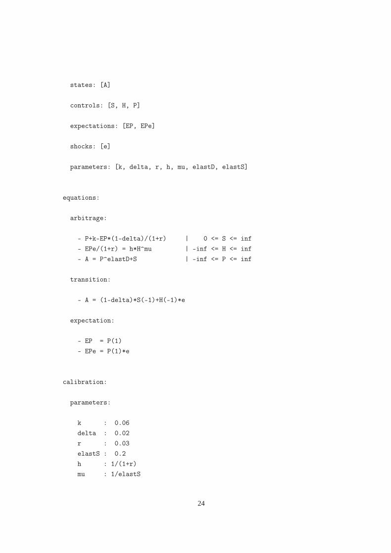
declarations:
states: [A]
controls: [S, H, P]
expectations: [EP, EPe]
shocks: [e]
parameters: [k, delta, r, h, mu, elastD, elastS]
equations:
arbitrage:
- P+k-EP*(1-delta)/(1+r) | 0 <= S <= inf
- EPe/(1+r) = h*H^mu | -inf <= H <= inf
- A = P^elastD+S | -inf <= P <= inf
transition:
- A = (1-delta)*S(-1)+H(-1)*e
expectation:
- EP = P(1)
- EPe = P(1)*e
calibration:
parameters:
k : 0.06
delta : 0.02
r : 0.03
elastS : 0.2
10

h : 1/(1+r)
mu : 1/elastS
elastD : -0.2
steady_state:
A : 1
S : 0
H : 1
P : 1
Observe that, this file, in addition to the definition of variables and equations, contains the values necessary
to calibrate the model.
3.3 Solving the storage model under Matlab
Once the Yaml file of a model has been written, which can been done using the Matlab editor, solving the
model involves following under Matlab these 4 steps:
i. Create the model structure in Matlab.
ii. Define the approximation space.
iii. Define a first-guess for the solver.
iv. Solve for the rational expectations equilibrium.
We now detail these steps for the case of our example model.
3.3.1 Create the model structure in Matlab
So far, Matlab does not know anything about the Yaml file and, even if it did, although the file is easy to
read and write for human, it is meaningless for Matlab. So we have to tell Matlab to use the Yaml file, and
convert it to a file format suitable for Matlab. This is done bythe functionrecsmodelinit, which creates
a structure containing the model, its shocks, parameters and steady-state as follows
Mu = 1;
sigma = 0.05;
model = recsmodelinit(’sto1.yaml’,struct(’Mu’,Mu,’Sigma’,sigma^2,’order’,7));
11

Deterministic steady state (equal to first guess)
State variables:
1
Response variables:
0 1 1
Expectations variables:
1 1
In creating the model structure, this function call also leads to calculation of the model deterministic steady
state using as a first guess the values provided in the Yaml file.
3.3.2 Define the approximation space
Having defined the model, we need to define the domain over which it will be approximated and the precision
of the approximation. The approximation space is defined by the functionrecsinterpinit, which requires
three inputs: the number of points on the grid of approximation, the lower bound, and the upper bound. In
this case, we choose 30 points for the grid, and bounds are defined relative to the steady-state value: half of
it for the lower bound and 80% above it for the upper bound.
[interp,s] = recsinterpinit(30,model.sss/2,model.sss*1.8);
This function creates the structureinterp, which contains all the information related to the approximation
space, and the variables, which is the grid of state variables.
3.3.3 Define a first-guess for the solver
The rational expectations solver has to be initialized froma good starting point to ensure convergence to the
rational expectations equilibrium. This can be done automatically by calculating the perfect foresight solu-
tion on the grid point corresponding to the stochastic problem. Using the two structures created previously,
this is done by the functionrecsFirstGuess:
[interp,x] = recsFirstGuess(interp,model,s,model.sss,model.xss,5);
3.3.4 Solve for the rational expectations equilibrium
Now we have all the elements required to solve the model: model definition, approximation space, and first
guess. All these elements have to be passed to the functionrecsSolveREE:
[interp,x] = recsSolveREE(interp,model,s,x);
12

Successive approximation
Iteration Residual
1 2.4E-001
2 4.2E-002
3 3.2E-002
4 2.7E-002
5 1.7E-002
6 6.6E-003
7 1.9E-003
8 5.1E-004
9 1.3E-004
10 3.2E-005
11 8.1E-006
12 2.0E-006
13 5.0E-007
14 1.2E-007
15 2.5E-008
16 1.6E-015
It outputsinterp, the interpolation structure that has been updated to contain the approximation of the
policy rules, andx the response variables on the grid.
3.3.5 Analyze the results
Once the model is solved, it is possible to analyze its behavior. This is done below through a stochastic
simulation that generates the main moments from the asymptotic distribution.
[~,~,~,~,stat] = recsSimul(model,interp,model.sss(ones(1000,1),:),200);
subplot(2,2,1)
xlabel(’Availability’)
ylabel(’Frequency’)
subplot(2,2,2)
xlabel(’Storage’)
ylabel(’Frequency’)
subplot(2,2,3)
xlabel(’Planned production’)
ylabel(’Frequency’)
subplot(2,2,4)
xlabel(’Price’)
ylabel(’Frequency’)
Statistics from simulated variables (excluding the first 20 observations):
13

Moments
Mean Std. Dev. Skewness Kurtosis Min Max %LB %UB
1.0167 0.0518 0.0190 2.9848 0.7767 1.2596
0.0158 0.0221 1.6203 5.3890 0 0.1842 25.7104 0
1.0010 0.0081 -1.4053 4.3248 0.9543 1.0074 0 0
1.0147 0.2011 1.9070 8.1329 0.6953 3.5376 0 0
Correlation
1.0000 0.8703 -0.8793 -0.9033
0.8703 1.0000 -0.9982 -0.5825
-0.8793 -0.9982 1.0000 0.5965
-0.9033 -0.5825 0.5965 1.0000
Autocorrelation
1 2 3 4 5
0.2152 0.0438 0.0024 -0.0037 -0.0066
0.2463 0.0536 0.0035 -0.0051 -0.0083
0.2449 0.0532 0.0034 -0.0053 -0.0081
0.1188 0.0188 -0.0009 -0.0033 -0.0043
0.8 1 1.2 1.40
1
2
3
4x 10
4
Availability
Fre
quen
cy
0 0.05 0.1 0.15 0.20
5
10
15x 10
4
Storage
Fre
quen
cy
0.94 0.96 0.98 1 1.020
5
10
15x 10
4
Planned production
Fre
quen
cy
0 1 2 3 40
2
4
6
8
10x 10
4
Price
Fre
quen
cy
figure
subplot(1,3,1)
14

plot(s,x(:,1))
xlabel(’Availability’)
ylabel(’Storage’)
subplot(1,3,2)
plot(s,x(:,2))
xlabel(’Availability’)
ylabel(’Planned production’)
subplot(1,3,3)
plot(s,x(:,3))
xlabel(’Availability’)
ylabel(’Price’)
0 1 20
0.1
0.2
0.3
0.4
0.5
0.6
0.7
0.8
0.9
Availability
Sto
rage
0 1 20.86
0.88
0.9
0.92
0.94
0.96
0.98
1
1.02
1.04
Availability
Pla
nned
pro
duct
ion
0 1 20
1
2
3
4
5
6
Availability
Pric
e
4 Convention to define stochastic rational expectations problem in RECS
4.1 Rational expectation models
There are several ways to define rational expectations models. RECS adopts a controlled-process conven-
tion in which the values taken by control, or response, variables are decided at each period based on the
values of state variables. The convention follows the framework proposed inFackler(2005), and used also
in Winschel and Krätzig(2010). A model can be defined by the following three equations, where time sub-
scripts are implicit for current-period variables, and next-period variables are indicated with the+ subscript,
15

while previous-period variables are indicated with the− subscript:
x(s)≤ x ≤ x(s) ⊥ f (s,x,z), where f : Rd+m+p → Rm, (6)
z = E[h(s,x,e+,s+,x+)] , whereh : Rd+m+q+d+m → Rp, (7)
s = g(s−,x−,e), whereg : Rd+m+q → Rd. (8)
Variables have been partitioned into state variables,s, response variables,x, and shocks,e. Response vari-
ables can have lower and upper bounds,x andx, which themselves can be functions of the state variables.
Expectations variables, denoted byz, are also defined, because they are necessary for solving themodel
considering the implemented algorithms.
The first equation is the equilibrium equation. It characterizes the behavior of the response variables given
state variables and expectations about the next period. Forgenerality, it is expressed as a mixed comple-
mentarity problem (MCP, if you aren’t familiar with the definition of MCP, see Section5). In cases where
response variables have no explicit lower and upper bounds,or have infinite ones, equation (6) simplifies to
a traditional equation:
0= f (s,x,z). (9)
The second equation (7) defines the expectations. The last equation, (8), is the state transition equation,
which defines how state variables are updated based on past responses, past states and contemporaneous
shocks.
4.2 Restrictions imposed by the RECS convention
Distinction between state variables and other variables In many models, it is possible to simplify the
state transition equations = g(s−,x−,e). For example, it is possible to haves = e if some shocks are not
serially correlated, ors = x− if the state is just a previous period response variables. Inthe latter case, one
might be tempted to reduce the number of variables in the model by introducing the lag response variable
directly in the equilibrium equation. This should not be done. A state variable corresponding to the lagged
response variable or to the realized shock has to be created.
One consequence is that lags can only appear in state transition equations, (8), and in no other equations.
Lags and leads RECS only deals with lags and leads of one period. For a model with lags/leads of more
periods, additional variables have to be included to reducethe number of periods.
In addition, leads can only appear in the equations defining expectations, (7). So no leads or lags should
ever appear in the equilibrium equations.
Timing convention In RECS, the timing of each variable reflects when that variable is decided/determined.
In particular, the RECS convention implies that state variables are determined by a transition equation that
16

includes shocks and so are always contemporaneous to shocks, even when shocks do not actually play a role
in the transition equation. This convention implies that the timing of each variable depends on the way the
model is written.
One illustration of the consequences of this convention is the timing of planned production in the competitive
storage model presented as a tutorial (Section3). Planned production,Ht , will only lead to actual production
in t + 1 and will be subject to shocks,εt+1, so it is tempting to use at + 1 indexing. However, since it is
determined int based on expectations of periodt +1 price, it should be indexedt.
4.3 An example
As an example, consider the competitive storage model presented in tutorial. It is composed of four equa-
tions:
St : St ≥ 0 ⊥ (1−δ )β Et (Pt+1)−Pt − k ≤ 0, (10)
Ht : β Et (Pt+1εt+1) = Ψ′ (Ht) , (11)
Pt : At = D(Pt)+St , (12)
At : At = Ht−1εt +(1−δ )St−1, (13)
whereS, H, P, andA respectively represent storage, planned production, price and availability.
There are three response variables:xt ≡ {St ,Ht ,Pt}, and three corresponding equilibrium equations (10)–
(12). These equations include two terms corresponding to expectations about periodt + 1: zt ≡
{Et (Pt+1) ,Et (Pt+1εt+1)}.
There is one state variable, availability:st ≡ {At}, which is associated to the transition equation (13). It
would have been perfectly legitimate to define the model withmore state variables, such as production and
stocks, since availability is the sum of both, and this wouldnot prevent the solver from finding the solution,
however, it is generally not a good idea. Since the solution methods implemented in RECS suffer from the
curse of dimensionality, it is important where possible to combine predetermined variables to reduce the
number of state variables.
Corresponding to RECS convention, this model is defined by the following three functions{ f ,h,g}:
f ≡
Pt + k− z1,t (1−δ )ββ z2,t −Ψ′ (Ht)
At −D(Pt)−St
(14)
h ≡
{
Pt+1
Pt+1εt+1
}
(15)
g ≡ {Ht−1εt +(1−δ )St−1} (16)
17

4.4 Solving a rational expectations model
What makes solving a rational expectations model complicated is that the equation (7), defining the expecta-
tions, is not a traditional algebraic equation. It is an equation that expresses the consistency between agents’
expectations, their information set, and realized outcomes.
One way to bring this problem back to a traditional equation is to find an approximation or an algebraic
representation of the expectations terms. For example, if it is possible to find an approximation of the
relationship between expectations and current-period state variables (i.e., the parameterized expectations
approach inden Haan and Marcet, 1990), the equilibrium equation can be simplified to
x(s)≤ x ≤ x(s) ⊥ f (s,x,Z (s,cz)) , (17)
whereZ (s,cz) approximates the expectationsz as a function ofs, andcz are the coefficients characterizing
this approximation. Using this approximation, equation (17) can be solved forx with any MCP solvers. So
the crux of solving rational expectations model is to find a good way to approximate the expectations.
The RECS solver implements various methods to solve rational expectations models and to find approxima-
tion for the expectations terms. See Section11 for a sketch of the algorithm.
5 Introduction to mixed complementarity problems
To be able to reliably solve models with occasionally binding constraints, all equilibrium equations should
be represented in RECS as mixed complementarity problems (MCP). Here, we present a short introduction
to this kind of problems. For more information, seeRutherford(1995), andFerris and Pang(1997).
5.1 Definition of a mixed complementarity problem
Complementarity problems can be seen as extensions of square systems of nonlinear equations that incorpo-
rate a mixture of equations and inequalities. Many economicproblems can be expressed as complementarity
problems. An MCP is defined as follows (adapted fromMunson, 2002):
Definition. (Mixed Complementarity Problem) Given a continuously differentiable functionF : Rn → Rn,
and lower and upper bounds
l ∈ {R∪{−∞}}n,
u ∈ {R∪{+∞}}n.
The mixed complementarity probleml ≤ x ≤ u ⊥ F(x) is to find ax ∈ Rn such that one of the following
18

holds for eachi ∈ {1, . . . ,n} :
Fi(x) = 0 andli ≤ xi ≤ ui, (18)
Fi(x) > 0 andxi = li, (19)
Fi(x) < 0 andxi = ui. (20)
To summarize, an MCP problem associates each variable,xi, to a lower bound,li, an upper bound,ui, and
an equation,Fi(x). The solution is such that ifxi is between its bounds thenFi(x) = 0. If xi is equal to its
lower (upper) bound thenFi(x) is positive (negative).
This format encompasses several cases. In particular, it iseasy to see that with infinite lower and upper
bounds, solving an MCP problem is equivalent to solving a square system of nonlinear equations:
−∞ ≤ x ≤+∞ ⊥ F(x) ⇔ F(x) = 0.
5.2 A simple example of mixed complementarity (model: CS1)
We consider here the traditional consumption/saving problem with borrowing constraint (Deaton, 1991).
This problem is solved as a demonstration, see problem CS1 inthe section Demos in the RECS documenta-
tion. A consumer with utility∑∞t=0 u(Ct)/(1+δ )t has a stochastic income,Yt and has to choose each period
how much to consume and how much to save. He is prevented from borrowing, but can save at the rater.
Without the borrowing constraint, his problem consists of choosing its consumptionCt such that it satisfies
the standard Euler equation:
u′ (Ct) =1+ r1+δ
Et[
u′ (Ct+1)]
.
The borrowing constraint implies the inequalityCt ≤ Xt , whereXt is the cash on hand available in periodt
and defined as
Xt = (1+ r) (Xt−1−Ct−1)+Yt .
When the constraint is binding (i.e.,Ct = Xt), the Euler equation no longer holds. The consumer would like
to borrow but cannot, so its marginal utility of immediate consumption is higher than its discounted marginal
utility over future consumption:
u′ (Ct)≥1+ r1+δ
Et[
u′ (Ct+1)]
.
Since the Euler equation holds when consumption is not constrained, this behavior can be summarized by
the following complementarity equation
Ct ≤ Xt ⊥1+ r1+δ
Et[
u′ (Ct+1)]
≤ u′ (Ct) .
19

5.3 When do complementarity problems arise?
In addition to encompassing nonlinear systems of equations, complementarity problems appear naturally in
economics. Although not exhaustive, we present here few situations that lead to complementarity problems:
• Karush-Kuhn-Tucker conditions of a constrained nonlinear program. The first-order conditions of
the following nonlinear programming problem minx f (x) subject tog(x) ≤ 0 andl ≤ x ≤ u can be
written as a system of complementarity equations:
l ≤ x ≤ u ⊥ f ′(x)−λg′(x), (21)
λ ≥ 0 ⊥ −g(x) ≥ 0, (22)
whereλ is the Lagrange multiplier on the first inequality constraint.
• Natural representation ofregime-switching behavior. Let us consider two examples.
– A variabley that is determined as a function of another variablex as long asy is superior to a
lower bounda. Put simply:y =max[a,λ (x)]. In MCP, we would write this asy ≥ a ⊥ y ≥ λ (x).
– A system of intervention prices in which a public stock is accumulated when prices decrease
below the intervention price and sold when they exceed the intervention price (see also the
demonstration problem in Section12.1) can be represented asS ≥ 0⊥ P−PI ≥ 0, whereS, P
andPI, respectively, are the public storage, the price and the intervention price.
• A Walrasian equilibrium can be formulated as a complementarity problem (Mathiesen, 1987) by
associating three sets of variables to three sets of inequalities: non-negative levels of activity are as-
sociated to zero-profit conditions, non-negative prices are associated to market clearance, and income
levels are associated to income balance.
5.4 Conventions of notations adopted for representing complementarity problems
To solve complementarity problems, RECS uses several solvers. The convention adopted in most MCP
solvers and used by RECS is the one used above in the MCP definition: superior or equal inequalities are
associated with the lower bounds and inferior or equal inequalities are associated with the upper bounds. So,
when defining your model, take care to respect this convention.
In addition, in Yaml files inequalities should not be writtenexplicitly. As an example, let’s consider these 5
20

MCP equations:
F(x) = 0, (23)
y ≥ a ⊥ G(y)≥ 0, (24)
z ≤ b ⊥ H (z)≤ 0, (25)
a ≤ k ≤ b ⊥ J (k) , (26)
l ≥ a ⊥ M (l)≤ 0. (27)
They would be written in a Yaml file as
- F(x)=0 | -inf<=x<=inf
- G(y) | a<=y<=inf
- H(z) | -inf<=z<=b
- J(k) | a<=k<=b
- -M(l) | a<=l<=inf
Note that it is necessary to associate lower and upper boundswith every variables, and the “perp” symbol
(⊥) is substituted by the vertical bar (|), which is much easier to find on a keyboard. So if there are no finite
bounds, one has to associate infinite bounds, as for equation(23). The last equation, (27), does not respect
the convention that associates lower bounds on variables with superior or equal inequality for equations, so,
when writing it in the Yaml file, the sign of the equation needsto be reversed.
5.5 Example: MCP representation of a price-band program (model: STO4)
Price-band policies constitute an excellent application for MCP modeling. Although this policy is simple to
express in words, it needs some reformulation and attentionto be expressed as an MCP problem.
This problem is analyzed in depth inMiranda and Helmberger(1988). This model is an extension of the
competitive storage model in which government intervenes by defending a price band through purchase and
sale of public storage. Here, we present an extension ofMiranda and Helmberger(1988) in which there is a
capacity constraint on the public stock level.
With a capacity constraint on public stock,S̄G, the behavior of a price-band obeys some simple principles.
When the price is above the floor price,PF, there is no accumulation of public stock,SG:
Pt > PF ⇒ ∆SGt ≤ 0. (28)
Likewise, when the price is below the ceiling price,PC, government does not sell stock:
Pt < PC ⇒ ∆SGt ≥ 0. (29)
21

When the capacity constraint is reached, the floor price is not defended and the price can decrease below it:
Pt < PF ⇒ ∆SGt = S̄G −SG
t−1. (30)
Finally, the ceiling price is not defended when the public stock is exhausted:
Pt > PC ⇒ ∆SGt =−SG
t−1. (31)
To express these four conditions as complementarity equations, we need to introduce two variables:∆SG+
and∆SG−, which refer to increases and decreases in public stock. Both are positive and bounded from above.
The increase in public stock is bounded from above by the remaining storage capacity, and the decrease in
public stock by the level of existing stocks. To defend the price-band, public stocks are managed by the four
conditions (28)–(31), which can be restated as two mixed complementarity equations:
0≤ ∆SG+t ≤ S̄G−SG
t−1 ⊥ Pt −PF, (32)
0≤ ∆SG−t ≤ SG
t−1 ⊥ PC−Pt. (33)
Equation (32) means that public stocks increase to prevent the price fromdecreasing below the floor price,
PF. The floor is defended until public stocks reach the limitS̄G. Equation (33) governs the decrease in public
stocks. They decrease to prevent the price from rising abovethe ceiling price,PC. The release of stocks is
constrained by the existing level of stocksSGt−1.
Market equilibrium and public stock transition are then defined by14
At = D(Pt)+St +∆SG+t −∆SG−
t , (34)
SGt = SG
t−1+∆SG+t −∆SG−
t . (35)
The recursive equilibrium under a price-band program is defined by the equilibrium equations (1), (3)
and (32)–(34), and the transition equations (4) and (35).
6 Setting Up a Rational Expectations Problem
6.1 Structure of RECS model files
6.1.1 Structure of a rational expectation models
Before starting to write the model file, you need to organize your equations as described in Section4. This
means that you need to identify and separate in your model thefollowing three group of equations:
Equilibrium equationsx(s) ≤ x ≤ x(s) ⊥ f (s,x,z). (36)
14Note that here, for simplicity, this model does not assume any depreciation during storage.
22

Expectations definitionz = E[h(s,x,e+,s+,x+)] . (37)
Transition equationss = g(s−,x−,e). (38)
When defining your model, it is important to try to minimize the number of state variables. Currently, RECS
relies for interpolation on grids constructed with tensor products, so the dimension of the problem increases
exponentially with the number of state variables. This implies that RECS should be used only to solve small-
scale models: more than three or four state variables may make the problems too large to handle. One way
of reducing the problem size is, whenever possible (as in thecompetitive storage model), to sum together
the predetermined variables that can be summed.
6.1.2 Structure of RECS model files
An RECS model can be written in a way that is quite similar to the original mathematical notations (as is
proposed in most algebraic modeling languages). The model file that must be created is called a Yaml file
(because it is written in YAML15 and has the.yaml extension). A Yaml file is easily readable by humans,
but not by Matlab. So the file needs to be processed for Matlab to be able to read it. This is done by the
functionrecsmodelinit, which uses a Python preprocessor,dolo-recs, to do the job.
RECS Yaml files require three basic components, written successively:
1. declarations – The blockdeclarations contains the declaration of all the variables, shocks and
parameters that are used in the model. Inside this block, there are five sub-blocks:states, controls,
expectations, shocks, andparameters with corresponding elements declarations.
2. equations – The blockequations declares the model’s equations.
3. calibration – The blockcalibration provides numerical values for parameters and a first-guess
for the deterministic steady-state.
Yaml file structure To illustrate a complete Yaml file let us consider how to writethe competitive storage
model in Yaml (available in filesto1.yaml):
# STO1.yaml Model definition file for the competitive storage model
# Copyright (C) 2011-2012 Christophe Gouel
# Licensed under the Expat license, see LICENSE.txt
declarations:
15http://yaml.org.
23
states: [A]
controls: [S, H, P]
expectations: [EP, EPe]
shocks: [e]
parameters: [k, delta, r, h, mu, elastD, elastS]
equations:
arbitrage:
- P+k-EP*(1-delta)/(1+r) | 0 <= S <= inf
- EPe/(1+r) = h*H^mu | -inf <= H <= inf
- A = P^elastD+S | -inf <= P <= inf
transition:
- A = (1-delta)*S(-1)+H(-1)*e
expectation:
- EP = P(1)
- EPe = P(1)*e
calibration:
parameters:
k : 0.06
delta : 0.02
r : 0.03
elastS : 0.2
h : 1/(1+r)
mu : 1/elastS
24

elastD : -0.2
steady_state:
A : 1
S : 0
H : 1
P : 1
Yaml files can be written with any text editor, including Matlab editor.
Yaml syntax conventions For the file to be readable, it is necessary to respect some syntax conventions:
• Association equilibrium equations/control variables/bounds: Each equilibrium equation must be
associated with a control variable. It really matters for equations with complementarity constraints. If
the equation is not a complementarity equation, the preciseassociation with a control variable does
not matter. The equation and its associated variable are separated by the symbol |. Control variables
must be associated with bounds, which can be infinite.
• Indentation: Inside each block elements of the same scope have to be indented using the same
number of spaces (do not use tabs). For the above example, inside thedeclarations block,states,
controls, expectations, shocks, andparameters are indented to the same level.
• Each equation starts with a dash and a space (“- ”), not to be confused with a minus sign. To avoid
confusion, it is possible instead to use two points and a space (“.. ”), or two dashes and a space
(“-- ”).
• Comments: Comments are introduced by the character#.
• Lead/Lag: Lead variables are indicatedX(1) and lag variablesX(-1).
• Timing convention:
– Transition equations are written by defining the new state variable at current time as a function
of lagged response and state variables:st = g(st−1,xt−1,et).
– Even if expectations are defined byzt = Et [h(st ,xt ,et+1,st+1,xt+1)], when writing them in a
Yaml file the shocks are not indicated with a lead. This can be seen in the example above where
Pt+1εt+1 is written asEPe = P(1)*e.
• Do not uselambda as a variable/parameter name, this is a restricted word.
• Write equations in the same order as the order of variables declaration.
• Yaml files are case sensitive.
25

6.2 Defining the model structure
Now the model should be written in a Yaml file, however Matlab does not know anything about the Yaml
file and, even if it did, although the file is easy for humans to read and write, it means nothing to Matlab. So
we have to tell Matlab to use the Yaml file and to convert it to a format suitable for Matlab. Also, we have
to provide additional information about the structure of shocks.
6.2.1 Convert the Yaml file and create the model structure
This task is done by the functionrecsmodelinit that calls a Python preprocessor, to convert the model
described in a Yaml file to a file readable by Matlab and RECS programs. In the conversion, it calculates
the analytic representation of all partial derivatives.
A simple call torecsmodelinit takes the following form:
model = recsmodelinit(’file.yaml’);
This call does two things:
• It convertsfile.yaml to filemodel.m, which contains the model definition in a Matlab readable
form but also all the derivatives of the equations, plus someadditional information such as the param-
eters values for calibration or a first guess for the steady state.
• It creates in Matlab workspace the structuremodel with two fields: the function name,func equal to
@filemodel, and the parameters values,params, if these latter have been provided in the Yaml file.
6.2.2 Shocks with a Gaussian distribution
If your shocks follow a Gaussian distribution, you can also define their structure when calling
recsmodelinit. It requires defining a structure with three fields characterizing the distribution mean, vari-
ance/covariance matrix, and order of approximation, with the call
model = recsmodelinit(’file.yaml’,...
struct(’Mu’,Mu,’Sigma’,Sigma,’order’,order));
HereMu is a size-q vector of the distribution mean,Sigma is a q-by-q positive definite variance/covariance
matrix, andorder is a scalar or a size-q vector equal to the number of nodes for each shock variable.
This function call creates at least three additional fields in the model structure:e a matrix of the nodes for
the shocks discretization;w the vector of associated probabilities; andfunrand an anonymous function that
can generate random numbers corresponding to the underlying distribution.
If a first-guess for the deterministic steady state has been provided,recsmodelinit attempts also to find
the deterministic steady state of the problem. If it finds it,it is displayed on screen and output as three fields
in the model structure:sss, xss, andzss for, respectively, the steady-state values of state, response and
expectations variables.
26

6.2.3 An example
Let us consider the example of the competitive storage model. The complete function call in sto1.m is:
Mu = 1;
sigma = 0.05;
model = recsmodelinit(’sto1.yaml’,struct(’Mu’,Mu,’Sigma’,sigma^2,’order’,7));
Deterministic steady state (equal to first guess)
State variables:
1
Response variables:
0 1 1
Expectations variables:
1 1
It is important to notice that variables names are not displayed here and will not be displayed in subsequent
steps. Variable names are used only in the symbolic model definition in the Yaml file. Once the Yaml file
has been processed, variables are merely ordered based on their original order in the Yaml file. In this case,
it means that, in the steady-state results above, for the response variables the first number is storage, the
second is planned production, and the third is price.
The model structure has the following fields:
disp(model)
func: @sto1model
params: [0.0600 0.0200 0.0300 0.9709 5 -0.2000 0.2000]
e: [7x1 double]
w: [7x1 double]
funrand: @(nrep)Mu(ones(nrep,1),:)+randn(nrep,q)*R
sss: 1
xss: [0 1 1]
zss: [1 1.0000]
27

6.3 Defining the interpolation structure
6.3.1 Define the interpolation structure
Following the previous two steps to completely define the problem, it remains only to define the domain
over which it will be approximated and the precision of the approximation.
Create the interpolation structure This task is done by the functionrecsinterpinit, which requires
at least three inputs: the number of points on the grid of approximation, the lower bounds and the upper
bounds of the grid.
The structure of the call torecsinterpinit is then
[interp,s] = recsinterpinit(n,smin,smax,method);
The inputs are as follows:n designates the order of approximation (if it is a scalar, thesame order is applied
for all dimensions),smin andsmax are size-d vectors of left and right endpoints of the state space, and the
(optional) stringmethod defines the interpolation method, either spline (’spli’, default), or Chebyshev
polynomials (’cheb’).
This function call returns two variables: the structureinterp, which defines the interpolation structure, and
the matrixs, which represents the state variables on the grid.
6.3.2 An example
We now define the interpolation structure for the competitive storage example. Using the model structure
defined in Section6.2, we choose bounds for availability 50% below and 80% above the steady-state value
(model.sss). Using 30 nodes and spline, the function call is:
[interp,s] = recsinterpinit(30,model.sss/2,model.sss*1.8);
The interpolation structure has the following fields:
disp(interp)
fspace: [1x1 struct]
Phi: [1x1 struct]
7 Steady state
In contrast to pertubation approaches, the deterministic steady state does not play an important role in finding
the rational expectations equilibrium with collocation methods, and thus with RECS. However, finding the
deterministic steady state proved very useful in the overall model building for
28

• Calibration;
• Definition of the approximation space;
• Calculation of a first guess using the corresponding perfectforesight problem;
• Checking model structure.
7.1 Steady state definition
The deterministic steady state is the state reached in the absence of shocks and ignoring future shocks.
Following the convention adopted in RECS (see Section4), the deterministic steady state is the set{s,x,z}
of state, response and expectations variables that solves the following system of equations
x(s) ≤ x ≤ x(s) ⊥ f (s,x,z), (39)
z = h(s,x,E(e) ,s,x), (40)
s = g(s,x,E(e)). (41)
7.2 Finding the steady state with RECS
Automatically when initializing model structure When writing a model file (see Section6.1, it is possi-
ble, at the end of the Yaml file in thecalibration block, to define an initial guess for finding the steady
state. When the model structure is created byrecsmodelinit, if the definition of the shocks is provided
to recsmodelinit, a Newton-type solver will attempt to find the steady state starting from the initial guess
provided in the model file. If a steady state is found, it is displayed in Matlab command window.
Manually Otherwise, the steady state can be found manually by feedingthe functionrecsSS with the
model and an initial guess for the steady state.
Both approaches rely on a Newton-type solver to find the steady state.
7.3 Uses of the deterministic steady state with RECS
Calibration Compared to the stochastic rational expectations problem,the deterministic steady state is
easy to find. It does not even require the definition of an interpolation structure. Since in practice it is often
close to the long-run average values of the stochastic problem, the steady state is useful for calibrating the
model so that, on the asymptotic distribution, the model canreproduce the desired long-run average (see
Section12.2).
Define the approximation space As the values of the state variables in the stochastic problem are often
located around the deterministic steady state, the steady state serves as a good reference point around which
the state space can be define. See Section6.3for more.
29

First guess calculation for the stochastic problem The rational expectations solver requires a good first
guess to ensure convergence to the solution. RECS proposes to provide a first guess by calculating the
perfect foresight problem corresponding to the stochasticproblem. The perfect foresight problem assumes
that the model converges in the long-run to its deterministic steady state. See next section for more.
Checking model structure Before solving the stochastic problem, even if there are no motives for using
the steady state, it is good practice to find it in order to ensure that the model written in the Yaml file behaves
as expected in this simple case.
8 First guess for the stochastic problem
The solution methods used in RECS to find the rational expectations equilibrium of a problem all rely on
nonlinear equation solvers that allow convergence only if the starting point is not too far from the solution.
Hence, the importance of a good first guess.
8.1 The perfect foresight problem as a first guess
RECS can attempt to calculate for you a first guess that is goodin most situations. It does it by calculating
the perfect foresight solution of the deterministic problem in which the shocks in the stochastic problem
have been substituted by their expectations:
x(s) ≤ x ≤ x(s) ⊥ f (s,x,z), (42)
z = h(s,x,E(e) ,s+,x+), (43)
s = g(s−,x−,E(e)). (44)
The solver for perfect foresight problems (functionrecsSolveDeterministicPb) assumes that the prob-
lem converges to its deterministic steady state after T periods (by default T=50). The perfect foresight
problem is solved for each grid point and the resultant behavior is used as a first guess for the stochastic
problem. This is done by the following call:
[interp,x] = recsFirstGuess(interp,model,s,sss,xss);
This function updates the interpolation structure,interp, with the solution of the perfect foresight problem
and outputs the value of the response variables on the grid,x.
Solving time As the perfect foresight problem is solved for each point of the grid and for T periods, this
step can take some time. In many cases, it should be expected that it may take more time to find a first guess
through the perfect foresight solution than to solve the stochastic problem from this first guess.
30

How good is this first guess? It depends on the model and the solution horizon. For most models, if the
state space has been properly defined (i.e., neither too small nor too large), this first guess is good enough to
allow the stochastic solver to converge.
The quality of the perfect foresight solution as a first guessdepends also on the model’s nonlinearity. For
models with behavior close to linear, the first guess can be extremely good. For example, in the stochastic
growth model the first guess leads to an initial deviation from rational expectations of 1E-5. So after a few
iterations, the solver converges to the solution. However,in the stochastic growth model with irreversible
investment, which is much more nonlinear, the residual whenstarting the stochastic solver from the first
guess is 1E-2. This is sufficient to achieve convergence, butit is still far from the true solution.
8.2 User-provided first guess
It is not necessary to use the deterministic problem as a firstguess. A first guess can be provided directly by
the user. In this case there is no need to call a function, but only to define a n-by-m matrixx that provides
the values of the m response variables for the n points on the grid of state variable. The matrixx should then
be supplied torecsSolveREE (see next section for more information).
9 Solve the rational expectations problem
9.1 The functionrecsSolveREE
Once the model, the interpolation structure and a first guesssolution have been defined, it is possible
to attempt to find the rational expectations equilibrium of the model. This is achieved by the function
recsSolveREE.
This is done by the following call
[interp,x] = recsSolveREE(interp,model,s,x,options);
This function call returns the interpolation structureinterp with new or updated fields. Following a suc-
cessful run ofrecsSolveREE, the fieldscx andcz are created or updated ininterp. They represent the
response and expectations variables interpolation coefficients, respectively. These coefficients are sufficient
to simulate the model. The second output is the matrixx of response variables on the grid.
The options structure defines the methods used to find the rational expectations equilibrium, as well as
other aspects of the solution process.
9.2 An example
First guess from the corresponding deterministic problem If the first guess is generated by the function
recsFirstGuess, interp already includes the fields of coefficientscx andcz corresponding to this first
31

guess, so it is not necessary to supply the value of the response variables on the grid. For the competitive
storage model, finding the first guess and solving the model involves the following call:
[interp,x] = recsFirstGuess(interp,model,s,model.sss,model.xss,5);
[interp,x] = recsSolveREE(interp,model,s);
Successive approximation
Iteration Residual
1 2.4E-001
2 4.2E-002
3 3.2E-002
4 2.7E-002
5 1.7E-002
6 6.6E-003
7 1.9E-003
8 5.1E-004
9 1.3E-004
10 3.2E-005
11 8.1E-006
12 2.0E-006
13 5.0E-007
14 1.2E-007
15 2.5E-008
16 1.7E-015
User-provided first guess If the first guess is provided by the user, there is no need to include the fields
cx or cz in interp. The user needs only to provide an n-by-m matrixx that contains the values of the m
response variables for the n points on the grid of state variable.
Our example is based on a simple first guess: storage is zero below steady-state availability and 70% of
availability in excess of steady state, planned productionis equal to its steady-state value and price is given
by the inverse demand function assuming that demand is equalto availability
elastD = model.params(6);
x = [max(0,0.7*s-model.sss) repmat(model.xss(2),size(s,1),1) s.^(1/elastD)];
[interp,x] = recsSolveREE(interp,model,s,x);
Successive approximation
Iteration Residual
1 2.1E+000
2 8.6E-001
3 3.6E-001
32

4 1.5E-001
5 5.4E-002
6 1.8E-002
7 5.0E-003
8 1.3E-003
9 3.4E-004
10 8.5E-005
11 2.1E-005
12 5.3E-006
13 1.3E-006
14 3.2E-007
15 7.9E-008
16 2.5E-015
With this simple model, even a naive first guess allows the solver to find the solution, however it significantly
decreases the precision of the first iteration.
10 Stochastic simulations
10.1 Running a simulation
Once the rational expectations equilibrium has been found,it is possible to simulate the model using the
functionrecsSimul with the following call:
[ssim,xsim] = recsSimul(model,interp,s0,nper);
wheremodel andinterp have been defined previously as the model and the interpolation structure.s0 is
the initial state andnper is the number of simulation periods.
s0 is not necessarily a unique vector of the state variables. Itis possible to provide a matrix of initial states
on the basis of which simulations can be run fornper periods. Even starting from a unique state, using this
feature will speed up the simulations.
Shocks The shocks used in the simulation can be provided as the fifth input to the function:
[ssim,xsim] = recsSimul(model,interp,s0,nper,shocks);
However, by default,recsSimul uses the functionfunrand defined in the model structure (see Section6.2)
to draw random shocks. If this function is not provided random draws are made from the shock discretization,
using the associated probabilities.
To reproduce previously run results, it is necessary to reset the random number generator using the Matlab
functionreset.
33

Asymptotic statistics If in the options the fieldstat is set to 1, or if five arguments are required as
output of recsSimul, then some statistics over the asymptotic distribution arecalculated. The first 20
observations are discarded. The statistics calculated arethe mean, standard deviation, skewness, kurtosis,
minimum, maximum, percentage of time spent at the lower and upper bounds, correlation matrix, and the
five first-order autocorrelation coefficients. In addition,recsSimul draws the histograms of the variables
distribution are drawn.
These statistics are available as a structure in the fifth output ofrecsSimul:
[ssim,xsim,esim,fsim,stat] = recsSimul(model,interp,s0,nper);
Since RECS does not retain the variable names, when displaying the statistics, the variables are organized
as follows: first state variables, followed by response variables, both of which follow the order of their
definition in the Yaml file.
10.2 Choice of simulation techniques
There are two main approaches to simulate the model once an approximated rational expectations equilib-
rium has been found.
Using approximated decision rule The first, and most common, method consists of simulating themodel
by applying the approximated decision rules recursively.
Starting from a knowns1, for t = 1 : T
xt = X (st ,cx) (45)
Draw a shock realizationet+1 from its distribution and update the state variable:
st+1 = g(st ,xt ,et+1) (46)
This is the default simulation method. It is chosen in the options structure by setting the fieldsimulmethod
to interpolation.
Solve equilibrium equations using approximated expectations The second main method uses the func-
tion being approximated (decisions rules, conditional expectations, or expectations function) to approximate
next-period expectations and solve the equilibrium equations to find the current decisions (in a time-iteration
approach). For example, if approximated expectations (z ≈ Z (s,cz)) are used to replace conditional expec-
tations in the equilibrium equation, the algorithm runs as follows:
Starting from a knowns1, for t = 1 : T , find xt by solving the following MCP equation using as first guess
xt = X (st ,cx)
x(st)≤ xt ≤ x(st) ⊥ f (st ,xt ,Z (st ,cz)) (47)
34
Draw a shock realizationet+1 from its distribution and update the state variable:
st+1 = g(st ,xt ,et+1) (48)
This simulation method is chosen in the options structure bysetting the fieldsimulmethod to solve.
The two approaches differ in their speed and precision. Simulating a model through recursive application of
approximated decision rules is very fast because it does notrequire solving nonlinear equations. The second
approach is slower because each period requires that a system of complementarity equations be solved.
However, its level of precision is much higher, because the approximation is used only for the expectations
of next-period conditions. The precision gain is even more important when decision rules have kinks, which
makes them difficult to approximate.Wright and Williams(1984), who first proposed the parameterized
expectations algorithm, suggest using the second method tosimulate the storage model.
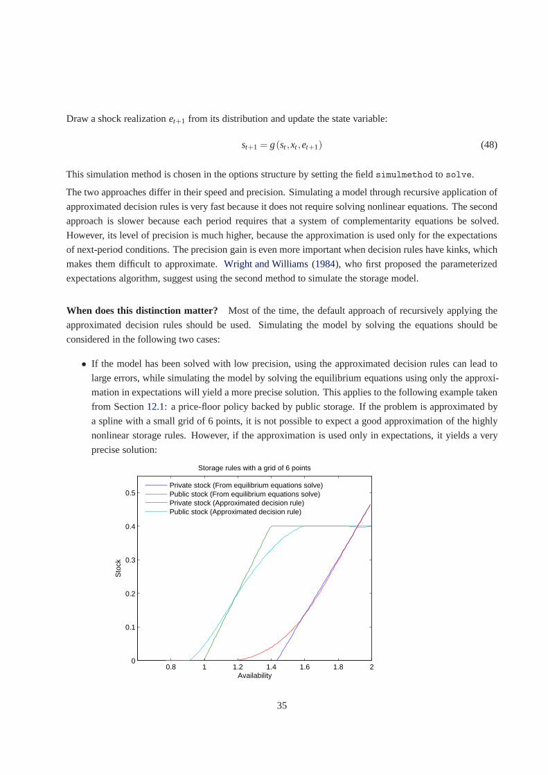
When does this distinction matter? Most of the time, the default approach of recursively applying the
approximated decision rules should be used. Simulating themodel by solving the equations should be
considered in the following two cases:
• If the model has been solved with low precision, using the approximated decision rules can lead to
large errors, while simulating the model by solving the equilibrium equations using only the approxi-
mation in expectations will yield a more precise solution. This applies to the following example taken
from Section12.1: a price-floor policy backed by public storage. If the problem is approximated by
a spline with a small grid of 6 points, it is not possible to expect a good approximation of the highly
nonlinear storage rules. However, if the approximation is used only in expectations, it yields a very
precise solution:
0.8 1 1.2 1.4 1.6 1.8 20
0.1
0.2
0.3
0.4
0.5
Availability
Sto
ck
Storage rules with a grid of 6 points
Private stock (From equilibrium equations solve)Public stock (From equilibrium equations solve)Private stock (Approximated decision rule)Public stock (Approximated decision rule)
35

• If you are interested in the percentage of time spent in various regimes, solving the equilibrium equa-
tions is the only way to achieve a precise estimate. Even whensolved with high precision, a simu-
lation using the approximated decision rules provides limited precision regarding the percentage of
time spent in each regime. Indeed, approximations using spline or Chebyshev polynomials fluctuate
around the exact value between collocation nodes. So between two nodes at which the model should
be at a bound, the approximated decision rule can yield a result very close to the bound without ac-
tually satisfying it. Below are the moments obtained from simulating the model in Section12.1with
both methods and with decision rules approximated on 30 nodes. The moments are quite similar, but
the approximated decision rules widely underestimate the time spent at the bounds:
Long-run statistics from equilibrium equations solve
Statistics from simulated variables (excluding the first 20 observations):
Moments
Mean Std. Dev. Skewness Kurtosis Min Max %LB %UB
1.2349 0.1199 -0.2424 2.3425 0.8457 1.5736
0.0007 0.0050 9.7021 115.6033 0 0.1133 96.4720 0
1.0026 0.0049 -0.7963 6.7106 0.9667 1.0160 0 0
1.0149 0.0523 3.5551 65.9633 0.7463 2.3121 0 0
0.2369 0.1141 -0.3280 2.0886 0 0.4000 2.3400 8.0010
Correlation
1.0000 0.2742 -0.8393 -0.4939 0.9947
0.2742 1.0000 -0.4928 -0.4930 0.1947
-0.8393 -0.4928 1.0000 0.6688 -0.7992
-0.4939 -0.4930 0.6688 1.0000 -0.4127
0.9947 0.1947 -0.7992 -0.4127 1.0000
Autocorrelation
1 2 3 4 5
0.8617 0.7473 0.6491 0.5629 0.4876
0.1079 0.0352 0.0165 0.0054 -0.0009
0.6710 0.4936 0.3824 0.3068 0.2551
Inf Inf Inf NaN -Inf
0.8712 0.7592 0.6618 0.5751 0.4981
Long-run statistics if simulated with approximated decision rules
Statistics from simulated variables (excluding the first 20 observations):
Moments
36

Mean Std. Dev. Skewness Kurtosis Min Max %LB %UB
1.2346 0.1200 -0.2457 2.3441 0.8458 1.5726
0.0008 0.0050 9.3978 112.0988 0 0.1125 48.8260 0
1.0026 0.0049 -0.7267 6.6960 0.9669 1.0163 0 0
1.0144 0.0511 4.3173 74.2896 0.7466 2.3105 0 0
0.2364 0.1140 -0.3384 2.0941 0 0.4000 1.6080 4.5290
Correlation
1.0000 0.3114 -0.8411 -0.4970 0.9948
0.3114 1.0000 -0.5348 -0.5403 0.2300
-0.8411 -0.5348 1.0000 0.6827 -0.7998
-0.4970 -0.5403 0.6827 1.0000 -0.4164
0.9948 0.2300 -0.7998 -0.4164 1.0000
Autocorrelation
1 2 3 4 5
0.8620 0.7476 0.6495 0.5633 0.4880
0.1818 0.0850 0.0502 0.0315 0.0214
0.6713 0.4938 0.3817 0.3067 0.2555
0.2894 0.1596 0.1008 0.0676 0.0524
0.8716 0.7597 0.6624 0.5757 0.4986
11 Sketch of the numerical algorithm
The numerical algorithms used in RECS are inspired byMiranda and Fackler(2002), Fackler(2005) and
Miranda and Glauber(1995). These are all projection methods with a collocation approach. Several meth-
ods are implemented, but we will only present here the default one: the approximation of response variables
behavior in a time iteration approach. As already explained, a model is characterized by three equations:
x(s) ≤ x ≤ x(s) ⊥ f (s,x,z), (49)
z = E[h(s,x,e+,s+,x+)] , (50)
s = g(s−,x−,e). (51)
One way to solve this problem is to find a function that is a goodapproximation for the behavior of the
37

response variables. We consider an approximation of response variables,
x ≈ X (s,cx) , (52)
wherecx are the parameters defining the spline or Chebyshev approximation. To calculate this approxima-
tion, we discretize the state space, and the approximation has to hold exactly for all points on the grid.
The expectations operator in equation (50) is approximated by a Gaussian quadrature, which defines a set
of pairs{el,wl} in which el represents a possible realization of shocks andwl is the associated probability.
Using this discretization, and equations (50)–(52), we can express the equilibrium equation (49) as
x(s)≤ x ≤ x(s) ⊥ f
(
s,x,∑l
wlh(s,x,el ,g(s,x,el) ,X (g(s,x,el) ,cx))
)
. (53)
For a given approximation,cx, and a givens, equation (53) is a function ofx and can be solved using a mixed
complementarity solver.
Once all the above elements are defined, we can proceed to the algorithm, which runs as follows:
1. Initialize the approximation,c(0)x , based on a first-guess,x(0).
2. For each point of the grid of state variables,si, solve forxi equation (53) using an MCP solver:
x(si)≤ xi ≤ x(si) ⊥ f
(
si,xi,∑l
wlh(
si,xi,el,g(si,xi,el) ,X(
g(si,xi,el) ,c(n)x
))
)
. (54)
3. Update the approximation using the new values of responsevariables,x = X
(
s,c(n+1)x
)
.
4. If ‖c(n+1)x − c(n)x ‖2 ≥ ε , whereε is the precision we want to achieve, then incrementn to n+1 and go
to step2.
Once the rational expectations equilibrium is identified, the approximation of the decision rules is used to
simulate the model.
This is only a sketch of the solution method. In fact, severalmethods are implemented. For example,
instead of using the simple updating rule in step3, a Newton, or inexact Newton, updating can be used when
feasible.
12 Examples of storage models
This section presents some examples of rational expectations models and their implementation in RECS. For
the simple competitive storage model, please see the tutorial in Section3.
38

12.1 Competitive storage with floor-price backed by public storage (model: STO2)
This model is a simple extension of the competitive storage model in which government attempts to defend a
floor price through public storage sale and purchase. The model presented here is close to one of the models
presented inWright and Williams(1988).
This policy is characterized by the following interventionrule, similar to that applying to price band in
Section5.5. All public stocks are sold if the price exceeds the intervention price:
Pt > PF ⇒ SGt = 0. (55)
Price can decrease below the floor if the capacity constraintS̄G is binding:
Pt < PF ⇒ SGt = S̄G. (56)
Public stock accumulation occurs to defend the floor price:
Pt = PF ⇒ 0≤ SGt ≤ S̄G. (57)
These three conditions can be written as one complementarity equation:
0≤ SGt ≤ S̄G ⊥ Pt −PF. (58)
Using the same assumptions as in the competitive storage model presented in Section3, the equations
defining this model are for equilibrium equations
St : St ≥ 0 ⊥ Pt + k− (1−δ )βEt (Pt+1)≥ 0, (59)
Ht : βEt (Pt+1εt+1) = hHtµ , (60)
Pt : At = Ptα +SS
t +SGt , (61)
SGt : 0≤ SG
t ≤ S̄G ⊥ Pt −PF, (62)
and for the transition equation
At : At = (1−δ )(
St−1+SGt−1
)
+Ht−1εt . (63)
It should be noted that this model has only one state variable, availability (At ), because the decision to
accumulate public stock depends only on current availability, not on past public stock.
A simulation of this model involves exactly the same steps asin the competitive storage model, so we do
not repeat them here; rather, we focus on welfare analysis issues. The reader can consult the filesto2.m in
RECS demonstration files to see the model resolution.
39

Welfare analysis Given that this is a simple model, we use it to illustrate welfare analysis in this dynamic
stochastic setting. Instantaneous social welfare,wt , here, is the sum of consumer’s surplus, producer’s
surplus, storer’s surplus and public cost:
wt =∫ P̄
Pt
D(p)dp+PtHt−1εt −Ψ(Ht)+ (1−δ )PtSt−1− (k+Pt)St +(1−δ )PtSGt−1− (k+Pt)SG
t . (64)
Ignoring in consumer’s surplus the term independent from policy choice and rearranging using (63), we
have
wt =−P1+α
t
1+α+PtAt −Ψ(Ht)− (k+Pt)
(
St +SGt
)
. (65)
Intertemporal welfare is given byWt = ∑∞i=0β iwt+i. It is clear that this infinite sum can be expressed as a
recursive equation:
Wt : Wt =−P1+α
t
1+α+PtAt −Ψ(Ht)− (k+Pt)
(
St +SGt
)
+β Et (Wt+1) . (66)
Similarly consumer welfare could be calculated recursively as
WCt : WC
t =−P1+α
t
1+α+β Et
(
WCt+1
)
. (67)
Calculating the welfare of the other agents is not as simple because it generally involves additional state vari-
ables. Indeed, producer’s welfare depends on past planned production as well as availability, and similarly,
storer’s welfare is a function of past private stock. So it isimportant to find a way to express these welfare
changes as a function only of availability. Since the private storer operates in expectations at zero profit,
its welfare can be reduced to the first-period benefit from holding stocks:(1−δ )P0S−1. Similarly, we can
decompose producer’s welfare between the first-period change and later changes: producer’s welfare at time
0 is equal toP0H−1ε0+W P0 , where
W Pt : W P
t = β Et (Pt+1εt+1)Ht −Ψ(Ht)+β Et(
W Pt
)
. (68)
We assume that public stocks are zero when the policy starts,so government benefits or losses from public
storage are
W Gt : W G
t = [(1−δ )β Et (Pt+1)− k−Pt]SGt +β Et
(
W Gt
)
. (69)
Equations (66)–(69) can be included in the model definition file (available in filesto2welf.yaml):
# STO2WELF.yaml Model definition file for the competitive storage with floor-price backed by public storage
# Copyright (C) 2011-2012 Christophe Gouel
# Licensed under the Expat license, see LICENSE.txt
declarations:
states: [A]
40

controls: [S, H, P, Sg, W, Wc, Wp, Wg]
expectations: [EP, EPe, EW, EWc, EWp, EWg]
shocks: [e]
parameters: [k, delta, r, h, mu, elastD, elastS, PF, Sgbar]
equations:
arbitrage:
- P+k-EP*(1-delta)/(1+r) | 0 <= S <= inf
- EPe/(1+r) = h*H^mu | -inf <= H <= inf
- A = P^elastD+S+Sg | -inf <= P <= inf
- P-PF | 0 <= Sg <= Sgbar
- W = -P^(1+elastD)/(1+elastD)+P*A-h*H^(1+mu)/(1+mu)-(P+k)*(S+Sg)+EW/(1+r) | -inf <= W <= inf
- Wc = -P^(1+elastD)/(1+elastD)+EWc/(1+r) | -inf <= Wc <= inf
- Wp = EPe*H/(1+r)-h*H^(1+mu)/(1+mu)+EWp/(1+r) | -inf <= Wp <= inf
- Wg = Sg*(EP*(1-delta)/(1+r)-P-k)+EWg/(1+r) | -inf <= Wg <= inf
transition:
- A = (1-delta)*(S(-1)+Sg(-1))+H(-1)*e
expectation:
- EP = P(1)
- EPe = P(1)*e
- EW = W(1)
- EWc = Wc(1)
- EWp = Wp(1)
- EWg = Wg(1)
calibration:
parameters:
k : 0.06
delta : 0.02
r : 0.03
elastS : 0.2
h : 1/(1+r)
mu : 1/elastS
elastD : -0.2
PF : 1.02
Sgbar : 0.4
41

steady_state:
A : 1
S : 0
H : 1
P : 1
Sg : Sgbar
W : (-P^(1+elastD)/(1+elastD)+P*A-h*H^(1+mu)/(1+mu)-(P+k)*(S+Sg))/(1-1/(1+r))
Wc : (-P^(1+elastD)/(1+elastD))/(1-1/(1+r))
Wp : (P*H/(1+r)-h*H^(1+mu)/(1+mu))/(1-1/(1+r))
Wg : Sg*(EP*(1-delta)/(1+r)-P-k)/(1-1/(1+r))
To analyze the welfare effect of introducing this policy, wehave to introduce the same welfare equations
in the competitive storage model. The model without policy and the model with policy are solved in the
Matlab filesto2welf.m:
function sto2welf
% STO2WELF Solves the floor-price model and calculates welfare changes
%% Pack model structures
Mu = 1;
sigma = 0.05;
model1 = recsmodelinit(’sto1welf.yaml’,struct(’Mu’,Mu,’Sigma’,sigma^2,’order’,7));
model2 = recsmodelinit(’sto2welf.yaml’,struct(’Mu’,Mu,’Sigma’,sigma^2,’order’,7));
%% Define approximation space
[interp1,s] = recsinterpinit(50,0.7,2);
interp2 = interp1;
%% Find a first guess through the perfect foresight solution
interp1 = recsFirstGuess(interp1,model1,s,model1.sss,model1.xss,5);
interp2 = recsFirstGuess(interp2,model2,s,model2.sss,model2.xss,5);
%% Solve for rational expectations (option: hide iterations)
[interp1,x1] = recsSolveREE(interp1,model1,s,[],struct(’display’,0));
[interp2,x2] = recsSolveREE(interp2,model2,s,[],struct(’display’,0));
%% Long-run simulation
[~,~,~,~,stat] = recsSimul(model1,interp1,ones(1E4,1),200);
[~,~,~,~,stat] = recsSimul(model2,interp2,ones(1E4,1),200);
%% Welfare change
42

sinit = [1 0.2];
[W1,W2] = WelfareCalculation([1 0.2]);
DW = W2-W1;
disp(’Welfare change:’)
disp(DW)
fid = fopen(’./Published/sto2welf.tex’,’w’);
fwrite(fid,latex([DW(2:end) DW(1)],’%0.4f’));
fclose(fid);
%% Plot social welfare against initial availability
n = 100;
res = zeros(n,1);
H0 = linspace(0.8,1.7,n);
for i=1:n
[W1,W2] = WelfareCalculation([H0(i) 0]);
res(i) = W2(1)-W1(1);
end
figure
plot(H0,res)
xlabel(’Initial availability’)
ylabel(’Change in social welfare’)
set(gcf,’Color’,’w’)
export_fig sto2welf.eps
function [Welf1,Welf2] = WelfareCalculation(sinit)
% sinit is the decomposition of initial state between production and private
% stock: [H*eps (1-delta)*S]
%% Simulate the model for a given initial state variable to get welfare values
[~,xsim1] = recsSimul(model1,interp1,sum(sinit),0);
[~,xsim2] = recsSimul(model2,interp2,sum(sinit),0);
P0 = [xsim1(3) xsim2(3)];
beta = 1/(1+model1.params(3));
%% Calculate welfare
Welf1 = [xsim1(4:5) P0(1)*sinit(1)+xsim1(6) P0(1)*sinit(2) 0]*(1-beta);
Welf2 = [xsim2(5:6) P0(2)*sinit(1)+xsim2(7) P0(2)*sinit(2) xsim2(8)]*(1-beta);
end
43
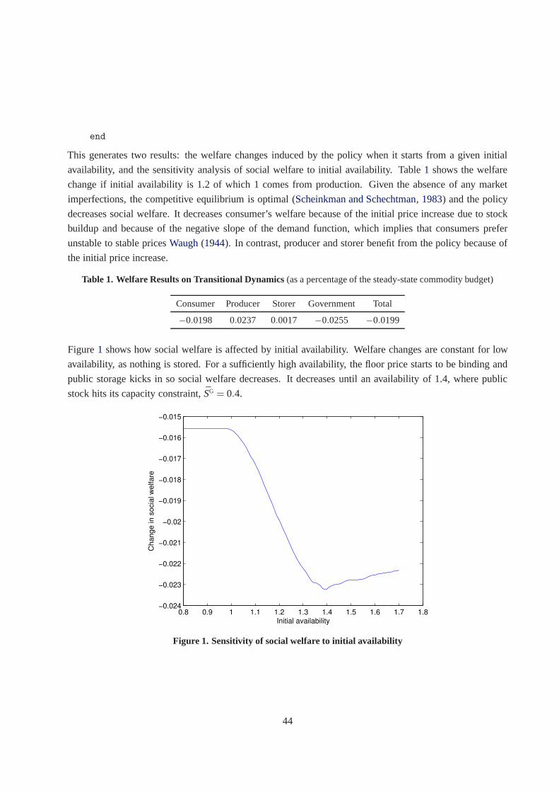
end
This generates two results: the welfare changes induced by the policy when it starts from a given initial
availability, and the sensitivity analysis of social welfare to initial availability. Table1 shows the welfare
change if initial availability is 1.2 of which 1 comes from production. Given the absence of any market
imperfections, the competitive equilibrium is optimal (Scheinkman and Schechtman, 1983) and the policy
decreases social welfare. It decreases consumer’s welfarebecause of the initial price increase due to stock
buildup and because of the negative slope of the demand function, which implies that consumers prefer
unstable to stable pricesWaugh(1944). In contrast, producer and storer benefit from the policy because of
the initial price increase.
Table 1. Welfare Results on Transitional Dynamics(as a percentage of the steady-state commodity budget)
Consumer Producer Storer Government Total
−0.0198 0.0237 0.0017 −0.0255 −0.0199
Figure1 shows how social welfare is affected by initial availability. Welfare changes are constant for low
availability, as nothing is stored. For a sufficiently high availability, the floor price starts to be binding and
public storage kicks in so social welfare decreases. It decreases until an availability of 1.4, where public
stock hits its capacity constraint,̄SG = 0.4.
0.8 0.9 1 1.1 1.2 1.3 1.4 1.5 1.6 1.7 1.8−0.024
−0.023
−0.022
−0.021
−0.02
−0.019
−0.018
−0.017
−0.016
−0.015
Initial availability
Change in s
ocia
l w
elfare
Figure 1. Sensitivity of social welfare to initial availability
44

12.2 Two-country storage-trade model (model: STO6)
In this section, we describe a model that is useful to analyzethe effects of the interaction between one
country’s domestic food market and the rest of the world: a two-country storage-trade model. This model
extends the competitive storage model to a situation with two locations, countriesa andb indicated by the
subscripti ∈ {a,b}.16 It assumes that in each country there is a demand for final consumption, production,
and competitive storage.
The countries are connected through trade, which occurs when the price difference covers the trade costs.
Trade is decided by the following spatial arbitrage condition:
Xit ≥ 0 ⊥ Pit +θ ≥ Pjt , for j 6= i, (70)
whereXit is the export from regioni, andθ is the per-unit transaction cost, inclusive of transport costs. This
implies that the prices in countryi fall within a moving band that is defined by country-j price and trade
costs:
Pjt −θ ≤ Pit ≤ Pjt +θ , for j 6= i. (71)
When adjusted for the subscriptsi and j, the model’s equations are similar to the single country case, ex-
cept for market equilibrium, which now accounts for trade. So the equations defining this model are for
equilibrium equations, fori ∈ {a,b} and j 6= i:
Sit : Sit ≥ 0 ⊥ Pit + k− (1−δ )βEt (Pit+1)≥ 0, (72)
Hit : βEt (Pit+1εit+1) = hiHitµ , (73)
Pit : Ait +X jt = γiPitα +Sit +Xit , (74)
Xit : Xit ≥ 0 ⊥ Pit +θ ≥ Pjt , (75)
wherehi andγi are country-specific scale parameters for supply and demand. The transition equations are,
for i ∈ {a,b}:
Ait : Ait = (1−δ )Sit−1+Hit−1εit . (76)
Calibration on real data While the previous models were calibrated on arbitrary data, here we show how
to calibrate a model on real data. For this, we followLarson et al.(2012) who calibrate a similar model
for the wheat market between the Middle East and North Africa(MENA) region and the rest of the world
(RoW).17
Storage models in the current literature are not calibratedbased on the time-series behavior of the corre-
sponding variables as is common for DSGE models. In addition, there is no procedure in the RECS toolbox
16The trade-and-storage model was first developed inWilliams and Wright(1991, Ch. 9), and was subsequently analyzed inMiranda and Glauber(1995), andMakki et al.(1996).
17In this case, the MENA region includes Algeria, Bahrain, Egypt, Iran, Iraq, Jordan, Kuwait, Lebanon, Libya, Morocco, Oman,Saudi Arabia, Syria, Tunisia, United Arab Emirates, and Yemen.
45

to make these calibrations automatically. Consequently, the calibration we present here aims at ensuring
that a benchmark equilibrium is reproduced at the deterministic steady state, and remaining behavioral pa-
rameters are set based on literature survey.
The calibration focuses on the steady state because it can besolved easily without having to solve for the
stochastic rational expectations equilibrium, and since in practice it is close to the long-run mean, calibrating
the steady state on average observed values should reproduce them as the long-run average of the model
variables. To help the calibration, note that we have no storage at steady state since prices are constant:
S∗i = 0, where∗ indicates variables at their steady-state values. Since Eεi = 1, we have alsoA∗i = H∗
i . As
can be seen in Table2, the MENA region is always importing wheat, which implies that
X∗RoW > 0, (77)
X∗MENA = 0, (78)
P∗MENA = P∗
RoW+θ . (79)
It is important to note that a storage model represents a stationary equilibrium, but the corresponding data
are not stationary. So, to calibrate the model, we start by removing the underlying trend. The detrended
data are presented in Table2. Since there is no stock at the steady state, quantities haveto be adjusted to
be consistent with a steady-state equilibrium. The steady-state MENA price is defined by assuming that the
price difference between the regions reflects transport costs, which is set at $35.55/ton based on a recent
survey (World Bank and FAO, 2012). Choosing a reference equilibrium point is not sufficient to assign a
value to every parameter. To pick up parameters that cannot be identified at the steady state (elasticities,
storage costs, discount rate), we rely on the literature. Weare guided by the literature on commodity price
dynamics, which shows that observed price volatility is consistent with relatively low demand elasticities
(Roberts and Schlenker, 2009, Cafiero et al., 2011), thus, we assume demand elasticity to be equal to−0.12,
which is toward the lower end of commonly used elasticities.We consider a supply elasticity of 0.2, in
line with commonly used supply elasticities for wheat.18 Interest rates and per unit storage charges are
assumed to be the same for each region at 5% per annum and $22.40 per ton per annum, respectively.
The storage costs are based on the findings from a recent WorldBank study on wheat markets in MENA
(World Bank and FAO, 2012).
Using these behavioral parameters and target values at the steady state, we can calculatehi andγi using
equation (73) and (74).
This model and its calibration are written in the Yaml filesto6MENA.yaml:
# STO6MENA.yaml Model definition file for a two-country storage-trade model with supply reaction (calibration
# Copyright (C) 2011-2012 Christophe Gouel
# Licensed under the Expat license, see LICENSE.txt
# Country a is MENA, and b is RoW
18See, for example, FAPRI’s elasticity database, available on the internet athttp://www.fapri.iastate.edu/tools/elasticity.aspx.
46

Table 2. Model calibration
MENA RoW
Calibration target at steady state
Consumption (million ton) 75.3 592.9Production (million ton) 40.2 628Price ($/ton) 211.55 176
Parameter
α −0.12β 0.9524γi 143.2 1102.7δ 0std(εi) 0.07 0.03θ 35.55µ 5hi 1.92E−6 1.72E−12k 22.4
Notes: Consumption, production and price in RoW targets aredetermined as 2011 trend values after applying a Holdrick-Prescottfilter (smoothing parameter of 400) to the underlying data (USDA, 2011, for consumption and production and World Bank, 2011,for price). RoW consumption is adjusted to ensure global market equilibrium. MENA price target is defined by adding transportcost to RoW price.
declarations:
states: [Aa, Ab]
controls: [Sa, Sb, Ha, Hb, Pa, Pb, Xa, Xb]
expectations: [EPa, EPb, EPea, EPeb]
shocks: [ea, eb]
parameters: [k, r, delta, ha, hb, mu, elastS, theta, elastD, gammaa, gammab, beta]
equations:
arbitrage:
.. Pa+k-EPa*(1-delta)/(1+r) | 0 <= Sa <= inf
.. Pb+k-EPb*(1-delta)/(1+r) | 0 <= Sb <= inf
.. EPea/(1+r) = ha*Ha^mu | -inf <= Ha <= inf
.. EPeb/(1+r) = hb*Hb^mu | -inf <= Hb <= inf
.. Aa+Xb = gammaa*Pa^elastD+Sa+Xa | -inf <= Pa <= inf
.. Ab+Xa = gammab*Pb^elastD+Sb+Xb | -inf <= Pb <= inf
47

.. Pa-Pb+theta | 0 <= Xa <= inf
.. Pb-Pa+theta | 0 <= Xb <= inf
transition:
.. Aa = (1-delta)*Sa(-1)+Ha(-1)*ea
.. Ab = (1-delta)*Sb(-1)+Hb(-1)*eb
expectation:
.. EPa = Pa(1)
.. EPb = Pb(1)
.. EPea = Pa(1)*ea
.. EPeb = Pb(1)*eb
calibration:
parameters:
k : 22.4
r : 0.05
beta : 1/(1+r)
delta : 0
elastS : 0.2
mu : 1/elastS
elastD : -0.12
theta : 35.55
gammaa : (Aa+Xb-Sa-Xa)/Pa^elastD
gammab : (Ab+Xa-Sb-Xb)/Pb^elastD
ha : Pa*beta/Ha^mu
hb : Pb*beta/Hb^mu
steady_state:
Aa : Ha
Ab : Hb
Sa : 0
Sb : 0
Ha : 40.2
Hb : 628
Pa : 211.55
Pb : 176
Xa : 0
Xb : Hb-592.9
It can be seen that the values entered for the parameters and first guess of the steady state may each be
48

function of the other, which facilitates model calibration.
The model is solved using the same commands as before, found in sto6MENA.m.
References
Adda, J. and Cooper, R. (2003).Dynamic Economics. Quantitative Method and Applications. Cambridge,
Massachusetts: The MIT Press.
Cafiero, C., Bobenrieth, E. S. A., Bobenrieth, J. R. A. and Wright, B. D. (2011). The empirical relevance of
the competitive storage model.Journal of Econometrics, 162(1), 44–54.
Deaton, A. (1991). Saving and liquidity constraints.Econometrica, 59(5), 1221–1248.
Deaton, A. and Laroque, G. (1992). On the behaviour of commodity prices.Review of Economic Studies,
59(1), 1–23.
Fackler, P. L. (2005). A MATLAB solver for nonlinear rational expectations models.Computational Eco-
nomics, 26(2), 173–181.
Fafchamps, M. (2003).Rural Poverty, Risk and Development. Edward Elgar Publishing.
Ferris, M. and Pang, J. (1997). Engineering and economic applications of complementarity problems.Siam
Review, 39(4), 669–713.
Gilbert, C. L. (1996). International commodity agreements: An obituary notice.World Development, 24(1),
1–19.
Gouel, C. (2011). Rules versus discretion in food storage policies, mimeo.
Gouel, C. (2013). Optimal food price stabilisation policy.European Economic Review, 57, 118–134.
Gouel, C. and Jean, S. (2012).Optimal Food Price Stabilization in a Small Open Developing Country. Policy
Research Working Paper 5943, The World Bank, URL:http://go.worldbank.org/23I9ACR4R0.
den Haan, W. J. and Marcet, A. (1990). Solving the stochasticgrowth model by parameterizing expectations.
Journal of Business & Economic Statistics, 8(1), 31–34.
Jayne, T. S. and Jones, S. (1997). Food marketing and pricingpolicy in Eastern and Southern Africa: A
survey.World Development, 25(9), 1505–1527.
Larson, D. F., Lampietti, J., Gouel, C., Cafiero, C. and Roberts, J. (2012).Food security and storage in the
Middle East and North Africa. Policy Research Working Paper Series 6031, The World Bank.
Makki, S. S., Tweeten, L. G. and Miranda, M. J. (1996). Wheat storage and trade in an efficient global
market.American Journal of Agricultural Economics, 78(4), 879–890.
Makki, S. S., Tweeten, L. G. and Miranda, M. J. (2001). Storage-trade interactions under uncertainty-
implications for food security.Journal of Policy Modeling, 23(2), 127–140.
Mathiesen, L. (1987). An algorithm based on a sequence of linear complementarity problems applied to a
walrasian equilibrium model: An example.Mathematical Programming, 37, 1–18.
49

Miranda, M. J. and Fackler, P. L. (2002).Applied Computational Economics and Finance. Cambridge: MIT
Press.
Miranda, M. J. and Glauber, J. W. (1995). Solving stochasticmodels of competitive storage and trade by
Chebychev collocation methods.Agricultural and Resource Economics Review, 24(1), 70–77.
Miranda, M. J. and Helmberger, P. G. (1988). The effects of commodity price stabilization programs.The
American Economic Review, 78(1), 46–58.
Munson, T. S. (2002). Algorithms and Environments for Complementarity. Ph.D. thesis, University of
Wisonsin—Madison.
Osborne, T. (2004). Market news in commodity price theory: Application to the Ethiopian grain market.
The Review of Economic Studies, 71(1), 133–164.
Park, A. (2006). Risk and household grain management in developing countries.Economic Journal,
116(514), 1088–1115.
Porteous, O. C. (2012). Empirical effects of short-term export bans: The case of african maize, mimeo.
Rashid, S., Gulati, A. and Cummings, R. W. (eds.) (2008).From Parastatals to Private Trade: Lessons from
Asian Agriculture. Baltimore, Md.; Washington D.C.: Johns Hopkins University Press ; International
Food Policy Research Institute.
Roberts, M. J. and Schlenker, W. (2009). World supply and demand of food commodity calories.American
Journal of Agricultural Economics, 91(5), 1235–1242.
Rutherford, T. F. (1995). Extension of GAMS for complementarity problems arising in applied economic
analysis.Journal of Economic Dynamics and Control, 19(8), 1299–1324.
Scheinkman, J. A. and Schechtman, J. (1983). A simple competitive model with production and storage.
The Review of Economic Studies, 50(3), 427–441.
Slayton, T. (2009).Rice Crisis Forensics: How Asian Governments Carelessly Set the World Rice Market
on Fire. Working Paper 163, Center for Global Development.
Waugh, F. V. (1944). Does the consumer benefit from price instability? The Quarterly Journal of Economics,
58(4), 602–614.
Williams, J. C. and Wright, B. D. (1991).Storage and Commodity Markets. New York: Cambridge Univer-
sity Press.
Winschel, V. and Krätzig, M. (2010). Solving, estimating, and selecting nonlinear dynamic models without
the curse of dimensionality.Econometrica, 78(2), 803–821.
World Bank and FAO (2012).The Grain Chain: Food Security and Managing Wheat Imports in Arab
Countries. Washington, DC.: World Bank.
Wright, B. D. (2001). Storage and price stabilization. In B.L. Gardner and G. C. Rausser (eds.)Marketing,
Distribution and Consumers, volume 1B, part 2 ofHandbook of Agricultural Economics, chapter 14, (pp.
817–861). Amsterdam: Elsevier.
Wright, B. D. and Williams, J. C. (1982). The economic role ofcommodity storage.The Economic Journal,
92(367), 596–614.
50

Wright, B. D. and Williams, J. C. (1984). The welfare effectsof the introduction of storage.The Quarterly
Journal of Economics, 99(1), 169–192.
Wright, B. D. and Williams, J. C. (1988). The incidence of market-stabilising price support schemes.The
Economic Journal, 98(393), 1183–1198.
51