Modeling and System Identification

Joe Hellerstein and Jie LiuMicrosoft

Jan. 14, 2008

CSE 590K: Analysis and Control of Computing Systems Using Linear Discrete-Time System Theory:

Last Time

• Basic Control System Architecture

• Typical Control Goals:– Regulatory control– Disturbance rejection– Optimization

• SASO properties: – Stability, Accuracy, Settling, Overshot

ControllerTarget

System

Reference

InputControl

Input

Measured

Output

Transduced

Output

Disturbance Input

Transducer

Queuing System

mService Requests

(arrivals)

Infinite size buffer (queue)

Service Completions

(departures)

l

Operation• Arrival of a service request

• Request enters service if buffer is empty• Enter queue if server is busy

• Completion of a service request• Next request in buffer enters the server• If buffer is empty, the system goes idle

M/M/1 Assumptions & Key Result• Assumptions

• Inter-arrival times are exponentially distributed• Service times are exponentially distributed

• Key result for steady state•N = expected number in system

lm

l

N

Today: Modeling

Signals, Systems, and Models

• Purpose of modeling

• Types of models

Model Construction

• Modeling from first principles

• Modeling from data

Hybrid System Models

Paper Discussion

Why bother modeling?

• Analysis

– prove formal properties (e.g. stability)

• Prediction

• Diagnostics

• Simulation

Queuing Model Revisit

mService Requests

(arrivals)

Infinite size queue

l Service Completions

(departures)

0 1 n

l l l l

m m m m

State is number of customers in the systemArrows indicate rate at which transitions occurArrival increases state by 1; departure decreases state by 1Probability of being in state n is pn

0n

nnpN

Good for steady-state analysis

Input-Output Models

• Examples of non-IO models

-- Automata -- Circuits

system

inputs outputs

Signals

• A signal is a function on a (usually ordered) set. Some signals may be partial functions.

Examples

• Continuous-Time Signals

– Functions on R+

• Discrete Events

– Partial functions on R+

• Discrete-Time signals

– Partial functions on R+

– Functions on N

• Signals on partially ordered sets

t

t

t (k)

t2

t1

t

Systems

• Systems are functions from signals to signals.– Note: Input and output signals do not necessarily have the same

domain or type.

• System composition

Serial: y = B(A(u))

Parallel: y = C(A(u1), B(u2))

Au

Bx y

A

B

C

u1

u2

y

A

B

yu

Feedback: y = A(B(y))

An I/O Model for a Queue

Service Requests

(arrivals)Service Completions

(departures)

queueu y

t0 t0

Is this model good for the purpose of controlling queue length?

What is it good for?

Another I/O Model for a Queue

Service Requests

(arrivals)Service Completions

(departures)

queueu y

t0 0

Check the queue length every T seconds.

T 2T 3T

2

54

T 2T 3T

1

3 3

t

Is this right?

)()()()1( kykukxkx

Difference equation

12

General View of Difference Equations

Term for the input-output models used General form

Relates current output to past outputs and inputs

)(...)1(

)(...)1()(

1

1

mkubkub

nkyakyaky

m

n

)( nky )1( ky

)( mku

)(ky

)1( ku

Order of a model: max(n,m)

…

…

Linear Time-Invariant

Linear Time-Invariance

• Linearity:

– f(x + y) = f(x) + f(y)

– f(αx) = αf(x) for all α

• Time-Invariance

– f(x(k+d))(k)=f(x)(k+d)

• Check

)(...)1(

)(...)1()(

1

1

mkubkub

nkyakyaky

m

n

LTI only if y starts from 0!

• The behavior of linear time invariant system is uniquely defined by it impulse response

Impulse Response

Non-Linear System Example

2( 1) ( ) ( ) ( )y k ay k y k u k

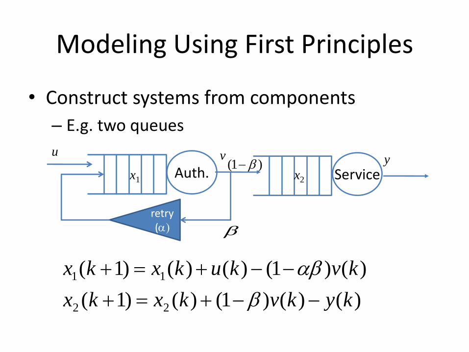
Modeling Using First Principles

• Construct systems from components

– E.g. two queues

Auth. Service

retry(a)

)()()1()()1(

)()1()()()1(

22

11

kykvkxkx

kvkukxkx

a

u

x1

v)1(

x2

y

Modeling Using First Principles

• Pros:

– Can be accurate

– Have strong system implications

• Cons:

– Requires strong domain knowledge

– Can be complicated

Modeling Using Data

• There is a whole field called machine learning!

• Pros:

– Weak dependency on domain knowledge

– Can be adaptive

• Cons:

– Requires data

– Only as good as data

19

Estimating Parameters of Difference Equations

• Statistical approach---Use linear least squares regression– Computations are simple

– Lots of software computes regression estimates (e.g., MatLab, Excel)

• Not a purely mechanical procedure– Need to determine a model structure (e.g. order)

– Need to validate inputs

– Need checks to ensure that models make sense

– Plots are very important tools

20

Linear Least Squares Regression Basics

y ax b Univariate linear regression equation:

LSR chooses a and b so as to minimize the sum of the square of the distances from data to line

y

x

*y (data point)

x*

*y (estimate)

Regression line

{EstimationError

21

Regression Metrics

Fraction of variance in data explained by the regression line.

2 [0,1]R

RMSE = Square root of the mean square of the estimation error

y

x

*y (data point)

x*

*y (estimate)

Regression line

{EstimationError

2

2

2

)(

)ˆ(

yy

yyR

i

ii

22

Examples of Regressions and Regression Metrics

23

Lies, Damn Lies, and Regression Metrics

Outlier distorts regression line Functional bias

Both models are very poor.

Estimating Parameters1. Choose order of model

Typically requires a multivariate regression model2. Run experiments in which control input is varied systematically3. Use least squares regression to estimate model parameters4. Assess the results

Offset MaxUsers Offset RIS)(ky)(ku Notes

Server

)1()1()( 11 kubkyaky0 0.5 1 1.5 2 2.5

x 106

0

50

100

150

200

250

300

350

Time (ms)

MaxUsers

MeasuredRIS

1 10.43, 0.47a b

Notes Example

Probe Further

• Recursive Least Square

– On-line parameter estimation

• Closed-loop system identification

• Reference: Lennart Ljung, System Identification: Theory for the User, Prentice Hall, 1999

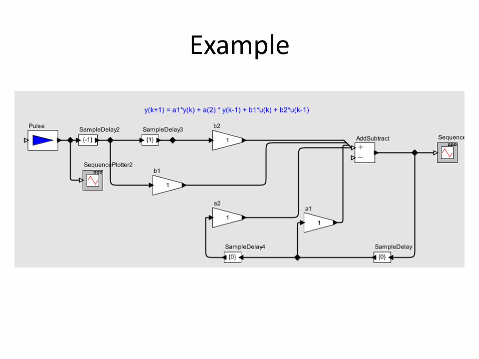
Example

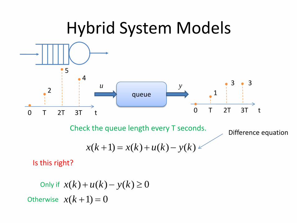
Hybrid System Models

queueu y

t0 0

Check the queue length every T seconds.

T 2T 3T

2

54

T 2T 3T

1

3 3

t

Is this right?

)()()()1( kykukxkx

Difference equation

Only if 0)()()( kykukx

Otherwise 0)1( kx

Hybrid System Models• Composition of state machines and differential(difference) equations.

“Normal”x(k+1) = x(k) + u(k)-y(k)

x(k+1) > 0x(k+1) < C

“Empty”x(k+1)=0

u(k) < =y(k)

x(k+1)=0

x(k+1)>=C | C:=2*C

discrete state

“continuous” dynamics

guard condition

invariance

action

A queue with increasing buffer size C

Behavior of Hybrid Systems

• a sequence of flows and jumps

• Properties about behavior– Safety: Do not enter “bad” states– Liveness: Behavior extends to infinity– Stability:

• Many properties are undecidedly in general

Be Careful about Hybrid Systems

• Zeno behavior

– Never-empty water tanks

• Stability is not composable

– switching between two stable systems can be unstable

w < v1 + v2

Probe Further

• Hybrid system lecture notes:http://robotics.eecs.berkeley.edu/~sastry/ee291e/lygeros.pdf

• Hybrid system modeling and simulation:

Google: HyVisual

Summary

• Many model structures for difference purposes

• Models can be constructed from first principles or data

• System identification for LTI systems

• Hybrid systems

Paper discussion

• Lu, Lu, Abdelzaher, Stankovic, Son, “Feedback Control Architecture and Design Methodology for Server Delay Guarantees in Web Servers” IEEE Tran. on Parallel and Distributed Systems, 17(9), Sept. 2006, pp.1014~1027