modeling and simulation of discrete-event systems || concepts and applications of parallel...

371

CHAPTER 12

Concepts and Applications of Parallel Simulation

Knowledge is a process of piling up facts; wisdom lies in their simplification.

—M. Fischer

12.1 INTRODUCTION

The terminologies used in this section are mostly from Fujimoto [2000], but the term parallel simulation is used somewhat differently. In Fujimoto, a simu-lation that executes on a set of computers confined to a single room is called a parallel simulation, whereas a distributed simulation executes on machines that are geographically distributed. In this book, a parallel simulation is defined as a simulation composed of a “collection of sequential simulations that exchange messages with each other” regardless of whether the computers are confined to a room or geographically distributed. In Fujimoto, a sequential simulation in the definition is referred to as a logical process (LP). A logical process has its own simulation clock. The key issue in parallel simulation is time synchronization to ensure that events are processed in a timestamp order when the logical processes are executed.

According to Fujimoto [2000], there exist two synchronization approaches: (1) one is conservative synchronization, which enforces all events be processed in timestamp order all the time; (2) the other is optimistic synchronization in which an out-of-order processing is allowed but the errors are recovered. Among the popular conservative synchronization methods are the centralized barrier method and the (distributed) null message method. The centralized barrier method, in which a controller LP is employed to implement the barrier for the simulator LPs, is as follows:

Modeling and Simulation of Discrete-Event Systems, First Edition. Byoung Kyu Choi and Donghun Kang.© 2013 John Wiley & Sons, Inc. Published 2013 by John Wiley & Sons, Inc.

372 ConCepts and appliCations of parallel simulation

1. The controller LP: determines when a barrier is reached and waits for messages from the simulator LPs. When a message is received from each simulator LP, it sends a “grant” message to the selected simulation LPs to release the barrier.

2. Simulator LPs: send a message to the controller LP and wait for a reply. When a “grant” message is received from the controller LP, safe events are executed.

In fact, the parallel simulation method with a centralized barrier has already been utilized quite extensively in this book. The state graph simulator intro-duced in Chapter 9 (Fig. 9.34 in Section 9.6.1) is a parallel simulation system where the Sync Manager plays the role of the controller LP. The object-oriented event graph simulator in Chapter 11 (Fig. 11.34 in Section 11.4.7) is also a parallel simulation system with the Simulation Coordinator playing the role of the controller LP.

A high-level architecture (HLA) is a general-purpose architecture for par-allel simulation systems. Using HLA, computer simulations can interact with other computer simulations regardless of the computing platforms. The inter-action between simulations is managed by a run-time infrastructure (RTI).

This chapter is organized as follows. A framework for direct workflow simu-lation based on parallel simulation is presented in Section 12.2. A brief descrip-tion of HLA/RTI is provided in Section 12.3, and an implementation example of parallel simulation HLA/RTI is introduced in Section 12.4.

12.2 PARALLEL SIMULATION OF WORKFLOW MANAGEMENT SYSTEM

This section presents a parallel simulation method with which the enactment service processes of a workflow management system (WfMS) can be simulated directly, i.e., without converting to a simulation model such as Petri nets.

12.2.1 Enactment Service Mechanism of WfMS

The basics of enactment service are briefly described using Fig. 12.1. For each instance of workflow, a process instance is created from its process definition model (PDM). Figure 12.1 shows a Process Instance consisting of seven activi-ties including Start and End activities. The completion of activity W1 will enable the two succeeding activities W2 and W3. At this point, the enactment server would provide the following sequence of enactment services:

1. Generates new workitems for the newly enabled activities W2 and W3.2. Sends out the new workitems W2 and W3 to their respective work-list

handlers to be processed by the participant.

parallel simulation of WorkfloW management system 373

3. Receives the completed workitem W2 from the work-list handler.4. Updates the state of the PI such that W2 becomes a completed activity.

Upon receiving the new workitem W2, (a) the work-list handler notifies it to its participant, and the participant (b) works on the workitem W2 for a time period of t2 and (c) reflects the results at the work-list handler so that the completed workitem is returned back to the enactment server. The communi-cations (i.e., sending new workitems and receiving completed workitems) between the enactment server and work-list handlers (or application handlers) are made based on the interface standards provided by a workflow manage-ment coalition (WfMC). For this purpose, the enactment server has a type of internal data called workflow relevant data that can be manipulated by work-list handlers and other applications via a set of standard API (application program interface) functions [WfMC 1995, 1998].

12.2.2 Framework of Parallel Simulation of WfMS

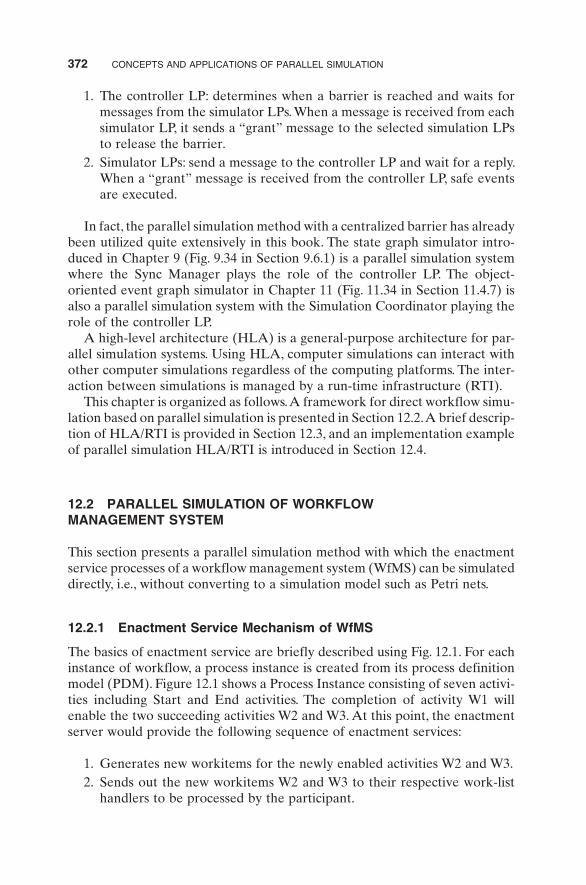
Shown in Fig. 12.2 are interactions among the software modules in the parallel simulation system. In this framework, data exchanges between the enactment server (Server) and participant simulators (Simulators) are made through the synchronization manager (Sync Manager). Thus, the role of the Sync Manager is to mediate the communications between the Server and Simulators while

Fig. 12.1. Enactment service mechanism of workflow management system (WfMS).

Send-out new workitems W2, W3 Receive completed workitem W2

[a] Notifies workitem (W2) arrival [c] Reflects “W2 completion”

[b] Processes W2 for a time period of t2 (processing time of W2)

Work-list Handler (Client)

Participants

W1 W3

W2

W4 Start W5 End

Completed Activity

Enactment Server

Process Instances (PI)

Enabled Activity

Enabled Activity

(0) Create process instances

Process Designer (PDM)

W2

Update state of PI

W3 W2

Generate new workitems

[[[b[[[[[[[[[[[[[[[[[[[[[[[[[[[[[[[[[[[[[[[[[[[[[[[[[


managing time synchronization. Here, the Sync Manager has all connection information of the Simulators that handle all new and completed workitems, and thus it handles all the “standard” enactment services provided by the Server.

At the beginning of an enactment service cycle, the Server generates new workitems {WN} and starts sending them one by one to the Sync Manager. In the meantime, the Sync Manager “looks into” the Server to get the number (μ) of newly generated workitems by using the API function ListWorkitems () specified in the WfMC standard [WfMC 1998]. Then, the following sequence of actions is taken by the software modules involved:

1. The Sync Manager passes each new workitem (WN) received from the Server to a pertinent Simulator while counting the number (m) of new workitems it has passed.

2. When m (number of passed workitems) becomes equal to μ (number of newly generated workitems), the Sync Manager broadcasts a message to every Simulator requesting to send its local next-event time (τL).

3. Each Simulator j reports τL (its local next-event time) to the Sync Manager.

4. The Sync Manager selects a Simulator j* that has the smallest next-event time (τG = Min {τL for all j}), and broadcasts the global next-event time (τG) and the selected Simulator ID (j*) to all Simulators.

5. The selected Simulator j* completes its workitem and advances its next-event time, and then returns the completed workitem (WC) back to the Sync Manager.

6. The Sync Manager passes the completed workitem (WC) to the Server, which in turn updates the pertinent process instance to initiate the next cycle of enactment service.

The above parallel simulation process employs a centralized barrier method of time synchronization with the Sync Manager playing the role of a controller LP. In the following sections, state graph models of the workflow simulation

Fig. 12.2. Interactions among the workflow simulation modules.

WN WC ( L, j)

Enactment Server {PI*}

Sync Manager

( G, j*)

Request

L

WN

WC

Participant Simulator j

Message unicasting

Data exchange

Message broadcast


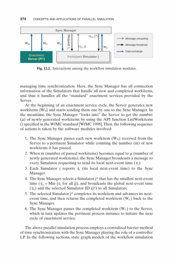
modules in Fig. 12.2 will be presented. Parameters and variables used in the state graph models are summarized in Table 12.1.

12.2.3 State Graph Modeling of an Enactment Server and Sync Manager

In this section, the behaviors of the enactment server and the Sync Manager are specified using the state graph modeling formalism presented in Chapter 9. A state graph model of the participant simulator will be presented in the next subsection. The materials presented in this section (Section 12.2) are mostly from the paper by Lee et al. [2010] where the term DEVS model was used in place of state graph model.

Shown in Fig. 12.3 is a simplified version of state graph model of the enactment server, which is a simple finite state machine having three states. It is initially in the Wait state and moves to the Processing state (Update PI & Generate {WN}) if the Start input is received. Once it has generated all the new workitems (for the enabled activities), it sends out the new workitems {WN} to the Sync Manager and moves to the Ready state. Then, it waits in the Ready state until it receives a completed workitem WC, and then moves back to the processing state. It should be noticed that the process-ing state may not generate a new workitem WN, in which case {WN} is a null

TABLE 12.1. Parameters and Variables Used in the State Graph Models

Name Description Name Description

a arrival time of workitem N total number of participant simulators

c completion time of workitem q number of workitems in queue

clock local simulation time of participant simulator

td time delay

G group size (number of people in the group)

WN new workitem

j ID number of a participant simulator

WC completed workitem

j* ID number of the selected participant simulator

π processing time of workitem

LLT list of local next-event times (τL) τL local next-event time of each participant simulator

m number of new workitems received

τG global next-event time

n number of participant simulators replied

μ total number of newly generated workitems


set, meaning that the state is changed to Ready without sending out any workitem.

Figure 12.4 shows a state graph model of our Sync Manager together with its interactions with the enactment Server and participant Simulators. In the figure, the operation sequence is numbered from (0) to (6). At the beginning of an enactment service cycle, the Sync Manager stays in the Wait for first WN state with m (the number of new workitems received) equal to zero. Then, (0) if a new workitem WN(π, j) is received from Server, (1) it moves to the Get μ state after sending WN(π) to Simulator j and setting m to one; otherwise, it moves to the Get μ state after a time delay of td. At the Get μ state, the Sync Manager obtains the value of μ = GetMu() (See Lee et al. 2010), and moves to the D1 state after setting μ = μ + m. Then, at the D1 state, (2) it goes to the Wait for next WN state and comes back until m is equal to μ. At this point (m ≡ μ), it moves to the Wait for τL state after sending the Request τL message to all Simulators and setting n (number of Simulators replied) to zero.

The Sync Manager waits in the Wait for τL state until (3) it receives the local next-event times (τL) from all Simulators (i.e., n ≡ N) while storing the value of each τL in the list of local next-event time LLT[j]. Then, (4) it selects a Simu-lator j* whose τL is the smallest, designating it as the global next-event time

Fig. 12.3. State graph model of the enactment server.

Ready {WN}!

Processing (Update PI &

Generate {WN})

WC?

Start? Wait

Enactment Server External transition

Internal transition

Msg? Input Msg

Msg! Output Msg

Fig. 12.4. State graph model of the Sync Manager.

(1) WN( )

Sync Manager

(3) ( L, j) (4) ( G, j*) (5) WC(a, , c)

a=arrival time, =processing time, c=completion time

( L, j)?

WC? WC!; m=0

Wait for WC

Wait for L

(n<N)

(n ≡ N)

(2) Req. L

Get µ (0)

(m<µ) (m≡µ)

(Req. L)! n=0

LLT[j] = L; n++

LLT=list of local next-event times( L)

(0) WN( , j) (6) WC(a, , c)

Participant Simulators {j} Enactment Server

Wait for first WN

(td)

D2 (0)

Wait for next WN WN( )!; m=1

µ = GetMu() + m

WN( , j)?

WN( )!; m++

WN( , j)?

d=Time delay, N=# of participant simulators, µ=# of new workitems

j*=arg Min{LLT(j)}; G= LLT(j*); G!

D1(0)


(τG), and moves to the Wait for WC state after broadcasting τG and j* to all Simulators. Finally, (5) if a completed workitem WC(a, π, c) is received from the selected Simulator j*, (6) the Sync Manager sends the WC to the Server and moves to the Wait for first WN state to start a next cycle of enactment service.

12.2.4 State Graph Modeling of Participant Simulators

Each single participant in the workflow management system is modeled as a single server system processing new workitems {WN (π)} received from the Sync Manager. Shown in Fig. 12.5 is a composite state graph model of the single server system consisting of three atomic models: Coordinator, Queue and Processor. Each Simulator communicates with the Sync Manager as follows: (1) new workitems WN (π) received are stored in the Queue and a selected workitem is processed by the Processor; (2) upon receiving a Req. τL message, (3) its local next-event time τL is returned back to the Sync Manager; (4) if global next-event time τG is granted to this Simulator, (5) the completed workitem Wc (a, π, c) is returned back to the Sync Manager.

12.2.5 Implementation of a Workflow Simulator

An existing workflow management system equipped with a Sync Manager and participant simulators can be used as a workflow simulator. Figure 12.6 shows the software structure of the workflow simulator: (1) a Workflow Engine

Fig. 12.5. State graph model of “single participant” simulator.

Simulator j

Idle

Queue WN (a, π)?

c= clock+π; WC (a, π, c); τL=c

Idle Wait for ask comp.

Processor

WN (a, π)

(ask comp.)?

WC!; done!; clock=τL; τL=∞

(1) WN(π)

Sync Manager

(3) (τL, j) (4) (τG, j*) (5) WC(a, π, c)

Coordinator

Wait for τG

WN?

WN!

WN(π)

(Req. τL)?

(ask τL)!

return τL

WC?

WC!

ask comp.

done

WC(a, π, c)

Processor busy WN? a=τG;

Enqueue(WN) (q≡0)

WN?

a=clock=τG; WN(a, π)!

(WN=Dequeue())!

(j≡ j*)

(2) Req. τL

Wait for τL

Wait for WC

(return τL)?

(τL, j)!

(τG, j*)?

(j≠ j*)

(ask comp.)!

ask τL

(ask τL)?, (return τL)!

(q>0)

q=# of workitems in queue, a=arrival time

(ask τL)? (return τL)!

done?

D1 ∆(0)

D2 ∆(0)

τL=local next-event time, c=completion time

clock=local simulation time

Wait for WN or Req. τL

: processing time; L/ G: local/global next-event time; a: arrival time; c: completed time


Connector is used to connect the components of the simulation system; (2) a Process Instance Generator is added to the simulation system to be used in generating process instances {PI*} from the process definition models (PDMs) defined at the Process Designer of the workflow management system; (3) a Process Monitor is also added to visualize the simulation process.

The Enactment Server provides enactment services to Participant Simula-tors through the Sync Manager. The workflow simulator was implemented as a prototype workflow simulator using a commercial workflow management system and an academic workflow management system, both of which are in compliance with the WfMC standards [WfMC 1995]. The Sync Manager and single and group participant simulators have been developed under a Micro-soft .NET Framework 3.5 environment using the C# programming language, and they are plugged into the workflow management systems via a workflow engine connector module [Lee et al. 2010].

12.3 OVERVIEW OF HIGH-LEVEL ARCHITECTURE/RUN-TIME INFRASTRUCTURE

As mentioned in the introduction, a high-level architecture (HLA) is a general-purpose architecture for parallel simulation systems, and the interactions between simulations are managed by a run-time infrastructure (RTI). HLA was mandated in September 1996 as the standard architecture for all modeling and simulation activities in the Department of Defense in the United States [Fujimoto 2000]. In HLA, a parallel simulation is referred to as a federation, and each individual sequential simulator as a federate. This section is based on the materials presented in the book by Kuhl et al. [2000] and in the lecture notes by Crosbie and Zenor [2006].

Fig. 12.6. Software structure of the workflow simulator.

Workflow Management System

Participant Simulators

Enactment Server {PI*}

Progress Monitor

(Animator)

Update Signal

Process Instance (PI) Generator

Sync Manager

Workflow Engine Connector Ask PI Create {PI*}

WN Send PI WC

WC

Session List (connections of participant simulators to enactment server)

WN

Process Instances {PI*} Process Designer

Participant Simulators

PDM

overvieW of HigH-level arCHiteCture/run-time infrastruCture 379

12.3.1 Basics of HLA/RTI

The objectives of HLA are to combine computer simulators into a larger simulation, or federation, to extend the simulation later by adding additional simulators, or federates, and to support component-based simulation develop-ment. In other words, it aims to enhance the reusability and interoperability of simulation models. Key components of HLA are HLA Rules, Interface Specification, and Object Model Template.

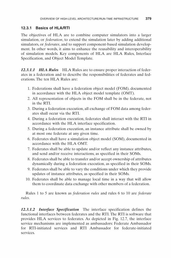
12.3.1.1 HLA Rules HLA Rules are to ensure proper interaction of feder-ates in a federation and to describe the responsibilities of federates and fed-erations. The ten HLA Rules are:

1. Federations shall have a federation object model (FOM), documented in accordance with the HLA object model template (OMT).

2. All representation of objects in the FOM shall be in the federate, not in the RTI.

3. During a federation execution, all exchange of FOM data among feder-ates shall occur via the RTI.

4. During a federation execution, federates shall interact with the RTI in accordance with the HLA interface specification.

5. During a federation execution, an instance attribute shall be owned by at most one federate at any given time.

6. Federates shall have a simulation object model (SOM), documented in accordance with the HLA OMT.

7. Federates shall be able to update and/or reflect any instance attributes, and send and/or receive interactions, as specified in their SOMs.

8. Federates shall be able to transfer and/or accept ownership of attributes dynamically during a federation execution, as specified in their SOMs.

9. Federates shall be able to vary the conditions under which they provide updates of instance attributes, as specified in their SOMs.

10. Federates shall be able to manage local time in a way that will allow them to coordinate data exchange with other members of a federation.

Rules 1 to 5 are known as federation rules and rules 6 to 10 are federate rules.

12.3.1.2 Interface Specification The interface specification defines the functional interfaces between federates and the RTI. The RTI is software that provides HLA services to federates. As depicted in Fig. 12.7, the interface service mechanisms are implemented as ambassadors: Federate Ambassador for RTI-initiated services and RTI Ambassador for federate-initiated services.


The interface specification (the set of APIs) for HLA services is divided into six management areas or RTI module groups. The six management areas are:

1. Federation management for creating federation execution and permitting a federate to join or to resign from the execution

2. Declaration management to allow federates to declare their intent to publish or subscribe to data

3. Object management to send and receive interactions; register a new object instance and update its attributes; and discover new instances and reflect updated attributes

4. Ownership management to grant/transfer of ownership of an instance-attribute

5. Data distribution management to control the producer-consumer rela-tionships among federates

6. Time management to allow federates to advance its logical time and control the delivery of timestamped events

12.3.1.3 Object Model Template (OMT) The OMT provides a standard for documenting HLA object model information. It defines the federation object model (FOM), the simulation or federate object model (SOM) and the management object model (MOM).

1. FOM introduces all shared data among federates: objects and interactions.

2. SOM describes salient characteristics (internal operations) of a federate.

3. MOM identifies objects and interactions used to manage a federation.

There are two types of shared data: interaction and object. An interaction is a collection of data (usually events) sent through the RTI to other federates. One federate sends an interaction; another receives it (and does not reside in the federation). Each interaction class has a set of named data called

Fig. 12.7. Interface service mechanisms of the RTI.

Run Time Infrastructure (RTI) RTI Ambassador RTI Ambassador

Federate-1

Federate Ambassador

Federate-n

Federate Ambassador Fede Service

Federate-Initiated Service

overvieW of HigH-level arCHiteCture/run-time infrastruCture 381

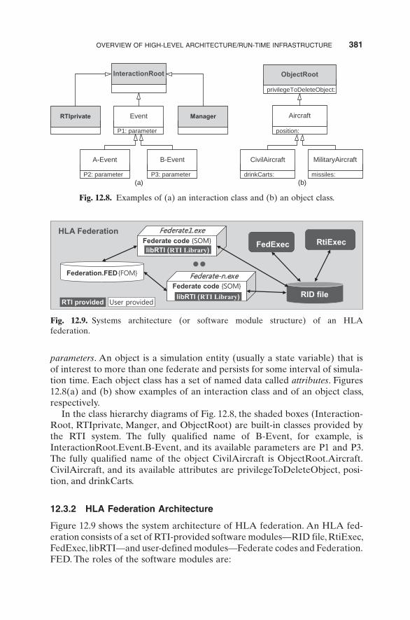
parameters. An object is a simulation entity (usually a state variable) that is of interest to more than one federate and persists for some interval of simula-tion time. Each object class has a set of named data called attributes. Figures 12.8(a) and (b) show examples of an interaction class and of an object class, respectively.

In the class hierarchy diagrams of Fig. 12.8, the shaded boxes (Interaction-Root, RTIprivate, Manger, and ObjectRoot) are built-in classes provided by the RTI system. The fully qualified name of B-Event, for example, is InteractionRoot.Event.B-Event, and its available parameters are P1 and P3. The fully qualified name of the object CivilAircraft is ObjectRoot.Aircraft.CivilAircraft, and its available attributes are privilegeToDeleteObject, posi-tion, and drinkCarts.

12.3.2 HLA Federation Architecture

Figure 12.9 shows the system architecture of HLA federation. An HLA fed-eration consists of a set of RTI-provided software modules—RID file, RtiExec, FedExec, libRTI—and user-defined modules—Federate codes and Federation.FED. The roles of the software modules are:

Fig. 12.8. Examples of (a) an interaction class and (b) an object class.

InteractionRoot

P1: parameter

Event

RTIprivate

Manager

P2: parameter

A-Event

P3: parameter

B-Event

privilegeToDeleteObject:

ObjectRoot

position:

Aircraft

drinkCarts:

CivilAircraft

missiles:

MilitaryAircraft

(a) (b)

Fig. 12.9. Systems architecture (or software module structure) of an HLA federation.

RID file

Federation.FED

FedExec

RtiExec

Federate code

Federate code HLA Federation

libRTI (RTI Library)

libRTI (RTI Library) RTI provided


1. The RTI initialization data (RID) file contains information needed to run the RTI.

2. The RtiExec (RTI executive) manages the creation and destruction of FedExec.

3. The FedExec (federation executive) allows federates to join and resign from the federation, and facilitates data exchanges among them.

4. The libRTI (RTI library) is used by federates to invoke various HLA services.

5. The Federation.FED (federation execution data) contains information derived from the FOM in the form of FDD (FOM document data) file.

6. A Federate.exe consists of federate code and libRTI. Federate code contains various local simulation objects including SOM.

In a physical configuration of a federation, a copy of each Federation. FED and RID file is bundled with each Fedreate.exe file in a local computer running the federate, and RtiExec and FedExec files reside in the “console” computer.

12.3.3 Overview of Federation Execution

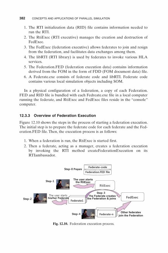
Figure 12.10 shows the steps in the process of starting a federation execution. The initial step is to prepare the federate code for each federate and the Fed-eration.FED file. Then, the execution process is as follows:

1. When a federation is run, the RtiExec is started first.2. Then a federate, acting as a manager, creates a federation execution

by invoking the RTI method createFederationExecution on its RTIambassador.

Fig. 12.10. Federation execution process.

implementation of a parallel simulation 383

3. The RTIambassador then reserves a name with RtiExec, and spawns a FedExec process, and that FedExec registers its communication address with RtiExec. The federation execution is underway.

4. Once a federation execution exists, other federates can join it. That RTIambassador consults RtiExec to get the address of FedExec, and invokes joinFederationExecution () on FedExec. Additional federates can join via the same process.

12.4 IMPLEMENTATION OF A PARALLEL SIMULATION WITH HIGH-LEVEL ARCHITECTURE/RUN-TIME INFRASTRUCTURE

This section aims to provide a beginner’s guide to the implementation example given in a book, which we call the HLA Book, by Kuhl et al. [2000]. The HLA Book provides an excellent coverage of the subject, and it may be easier for a beginner to understand the contents of the book after reading this section. This section begins with an overall description of the “sushi boat” restaurant system presented in Chapter 4 of the HLA Book.

12.4.1 The Sushi Restaurant Federation

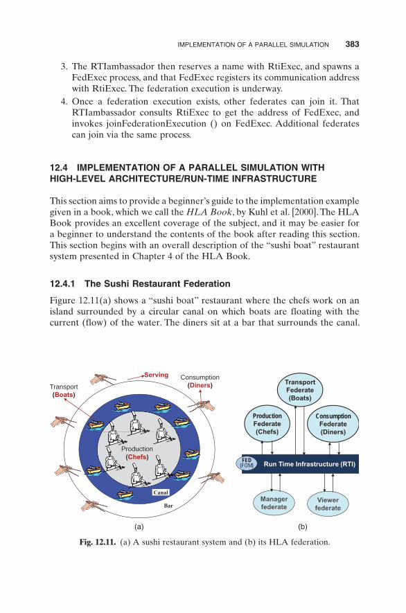
Figure 12.11(a) shows a “sushi boat” restaurant where the chefs work on an island surrounded by a circular canal on which boats are floating with the current (flow) of the water. The diners sit at a bar that surrounds the canal.

Fig. 12.11. (a) A sushi restaurant system and (b) its HLA federation.

Canal

Production (Chefs)

Transport (Boats)

Consumption (Diners)

Run Time Infrastructure (RTI)

Manager federate

Production Federate (Chefs)

Transport Federate (Boats)

Consumption Federate (Diners)

Viewer federate

FED (FOM)

Serving

Bar

(a) (b)


As the chefs prepare servings, they place them on rectangular plates; when they have finished a batch of servings, which may fill several plates, the chefs place the plates on empty boats as they float by. Diners remove the plate of their choice as the boat comes by and enjoy it. The chefs are called a produc-tion subsystem, the boats a transport subsystem, and the diners a consumption subsystem.

Figure 12.11(b) shows the HLA federation of the sushi restaurant system consisting of five federates and the RTI including a FED file. The three feder-ates corresponding to the three subsystems of the restaurant are called sub-system federates: Production federate, Transport federate, and Consumption federate. The Manager federate is used in managing the federation execution, and the Viewer federate acts as a passive recipient; its role is to display of simulation data from the rest of the federation. The FED (also called Federa-tion.FED) file contains the federation object model (FOM). As mentioned in Section 12.3.2 (Fig. 12.9), an HLA federation consists of a number of files in addition to the federates and FED file. However, only the federates and FED file need to be prepared by the federation designer.

12.4.2 Preparation of an FED File

As was shown in Fig. 12.11(a), there are four types of objects in the restaurant system: Servings, Boats, Chefs, and Diners. Figure 12.12(a) shows an object class tree specifying the restaurant objects. The root of the object class tree is

Fig. 12.12. (a) Object class tree and (b) interaction class tree.

ObjectRoot

privilegeToDeleteObject : String

Restaurant

position: Position

Serving

type : sushiTypeEnumeration

Boat

spaceAvailable : boolean cargo : String

Actor

servingName : String

Chef chefState : chefStateEnumeration

Diner dinerState : dinerStateEnumeration

InteractionRoot

Manager SimulationEnds TransferAccepted

servingName : String

(a)

(b)


called ObjectRoot. At the leaf level of the hierarchy are the four object classes: Serving, Boat, Chef, and Diner. The Actor class serves as a place to define the attribute servingName that is in common for Chef and Diner. The attributes chefState and dinerState are conceptually enumerations and will both be represented in Java as int.

Figure 12.12(b) shows a class tree for interactions. An interaction is a simu-lated occurrence (or event) that occurs at a point in time and does not persist. All interaction classes are subclasses of InteractionRoot. The TransferAc-cepted interaction has a parameter of servingName. It is a message sent from the Transport federate to the Production federate to signal a Boat’s acceptance of a Serving. SimulationEnds is a message sent from the Consumption federate to other federates signaling the end of simulation. It is a subclass of Manager because it is a user-extension of the management object model (MOM).

Figure 12.13 shows a FED file containing the object class tree and interac-tion class tree given in Fig. 12.12. Observe in the FED file that each class attribute and each interaction class are appended by modifiers reliable time-stamp or reliable receive. The choices of the communication network over which the messages (class attributes and interaction classes) are sent are either reliable or best-effort. A reliable communication guarantees that the data will be delivered or an exception will be indicated. The choices of message-delivery ordering are either timestamp or receive. In a timestamp order (TSO), the arrival of timestamped messages is sequenced in accordance with logical time;

Fig. 12.13. FED file for the object and interaction class trees in Fig. 12.12.

(FED ;; Defining object classes and interaction classes (Federation restaurant_1) ;; we choose this tag (FEDversion v1.3) ;; required; specifies RTI spec version (spaces ;; we define no routing spaces ) ( objects (class ObjectRoot ;; required (attribute privilegeToDeleteObject reliable timestamp) (class RTIprivate) (class Restaurant (attribute position reliable timestamp) (class Serving (attribute type reliable timestamp) ) (class Boat (attribute spaceAvailable reliable timestamp) (attribute cargo reliable timestamp) ) (class Actor (attribute servingName reliable timestamp) (class Chef (attribute chefState reliable timestamp) ) (class Diner (attribute dinerState reliable timestamp) ) ) ) ;; end of Restaurant (class Manager …) ) ;; end ObjectRoot ) ;; end Objects ( interactions (class InteractionRoot reliable timestamp (class TransferAccepted reliable timestamp (parameter servingName) ) (class RTIprivate reliable timestamp) (class Manager reliable receive (class SimulationEnds reliable receive) …) ;; end InteractionRoot ) ;; end interactions ) ;; end FED


in a receive order, the messages are delivered as they arrive without regard to logical time. In the FED file, both ObjectRoot and InteractionRoot have a required subclass called RTIprivate (not shown in Fig. 12.12) to be used by RTI implementers. It must be present but cannot be extended (subclasses) by a federation designer. ObjectRoot has another required subclass called Manager. It is the root of a further tree that defines the object portion of the Management Object Model (MOM). All the subclasses of Manager that you see in the sample FED files are required to be there.

12.4.3 Preparation of the Federate Code (of the Production Federate)

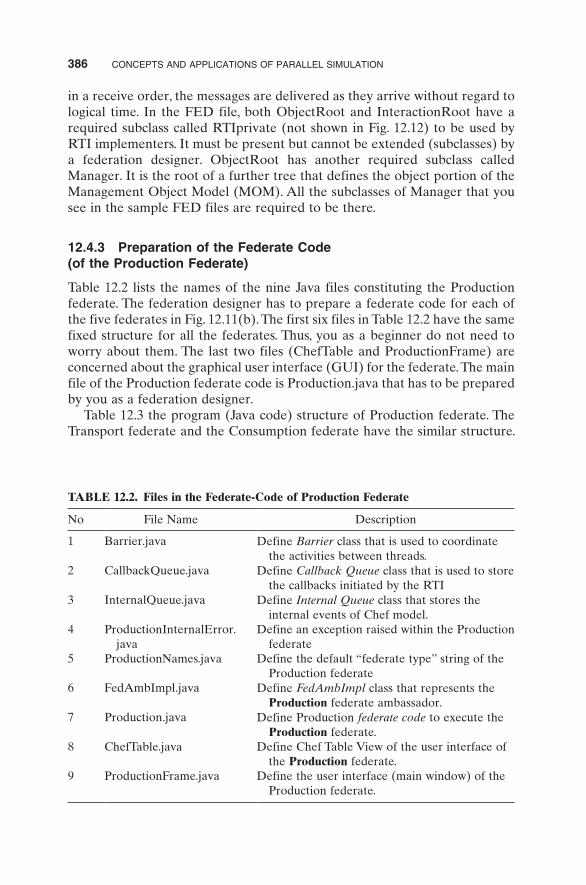
Table 12.2 lists the names of the nine Java files constituting the Production federate. The federation designer has to prepare a federate code for each of the five federates in Fig. 12.11(b). The first six files in Table 12.2 have the same fixed structure for all the federates. Thus, you as a beginner do not need to worry about them. The last two files (ChefTable and ProductionFrame) are concerned about the graphical user interface (GUI) for the federate. The main file of the Production federate code is Production.java that has to be prepared by you as a federation designer.

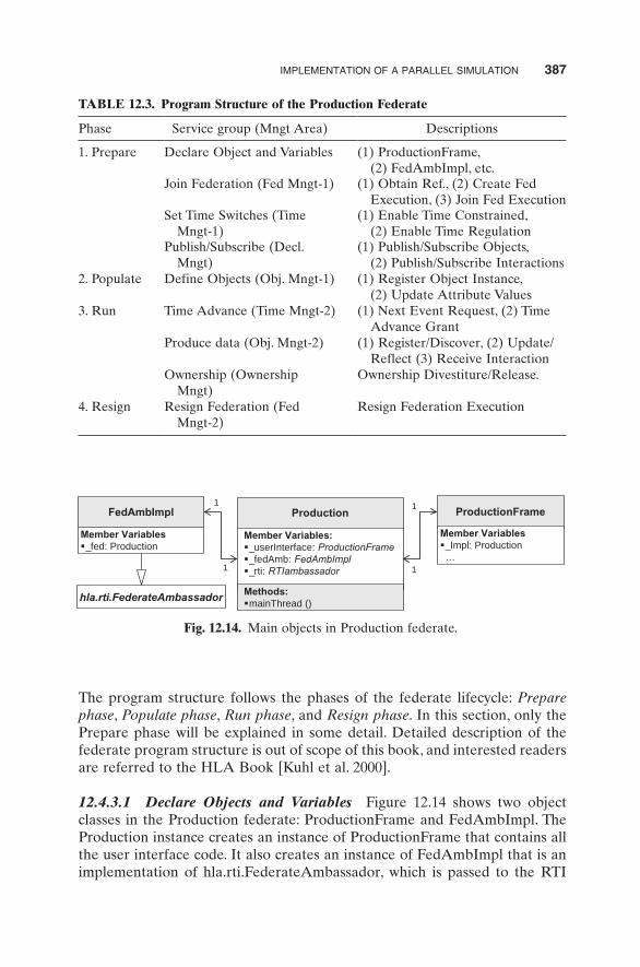
Table 12.3 the program (Java code) structure of Production federate. The Transport federate and the Consumption federate have the similar structure.

TABLE 12.2. Files in the Federate-Code of Production Federate

No File Name Description

1 Barrier.java Define Barrier class that is used to coordinate the activities between threads.

2 CallbackQueue.java Define Callback Queue class that is used to store the callbacks initiated by the RTI

3 InternalQueue.java Define Internal Queue class that stores the internal events of Chef model.

4 ProductionInternalError.java

Define an exception raised within the Production federate

5 ProductionNames.java Define the default “federate type” string of the Production federate

6 FedAmbImpl.java Define FedAmbImpl class that represents the Production federate ambassador.

7 Production.java Define Production federate code to execute the Production federate.

8 ChefTable.java Define Chef Table View of the user interface of the Production federate.

9 ProductionFrame.java Define the user interface (main window) of the Production federate.


The program structure follows the phases of the federate lifecycle: Prepare phase, Populate phase, Run phase, and Resign phase. In this section, only the Prepare phase will be explained in some detail. Detailed description of the federate program structure is out of scope of this book, and interested readers are referred to the HLA Book [Kuhl et al. 2000].

12.4.3.1 Declare Objects and Variables Figure 12.14 shows two object classes in the Production federate: ProductionFrame and FedAmbImpl. The Production instance creates an instance of ProductionFrame that contains all the user interface code. It also creates an instance of FedAmbImpl that is an implementation of hla.rti.FederateAmbassador, which is passed to the RTI

TABLE 12.3. Program Structure of the Production Federate

Phase Service group (Mngt Area) Descriptions

1. Prepare Declare Object and Variables (1) ProductionFrame, (2) FedAmbImpl, etc.

Join Federation (Fed Mngt-1) (1) Obtain Ref., (2) Create Fed Execution, (3) Join Fed Execution

Set Time Switches (Time Mngt-1)

(1) Enable Time Constrained, (2) Enable Time Regulation

Publish/Subscribe (Decl. Mngt)

(1) Publish/Subscribe Objects, (2) Publish/Subscribe Interactions

2. Populate Define Objects (Obj. Mngt-1) (1) Register Object Instance, (2) Update Attribute Values

3. Run Time Advance (Time Mngt-2) (1) Next Event Request, (2) Time Advance Grant

Produce data (Obj. Mngt-2) (1) Register/Discover, (2) Update/Reflect (3) Receive Interaction

Ownership (Ownership Mngt)

Ownership Divestiture/Release.

4. Resign Resign Federation (Fed Mngt-2)

Resign Federation Execution

Fig. 12.14. Main objects in Production federate.

FedAmbImpl

Member Variables _fed: Production

Production

Member Variables: _userInterface: ProductionFrame _fedAmb: FedAmbImpl _rti: RTIambassador

…

hla.rti.FederateAmbassador Methods: mainThread ()

1

1

ProductionFrame

Member Variables _Impl: Production …

1

1


when the federate joins. Callbacks from the RTI are invoked on FedAmbImpl, which in turn calls methods in the Production instance. The Production class contains the mainThread () method that contains the rest of the federate code. The mainThread () holds the references to other data structures and objects, and all the calls to RTIambassador occur in its code.

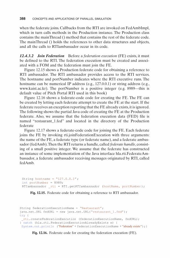
12.4.3.2 Join Federation Before a federation execution (FE) exists, it must be defined to the RTI. The federation execution must be created and associ-ated with a FOM and the federation must join the FE.

Figure 12.15 shows a Production federate code for obtaining a reference to RTI ambassador. The RTI ambassador provides access to the RTI services. The hostname and portNumber indicates where the RTI executive runs. The hostname can be numerical IP address (e.g., 127.0.0.1) or string address (e.g., www.kaist.ac.kr). The portNumber is a positive integer (e.g. 8989—this is default value of Pitch Portal RTI used in this book)

Figure 12.16 shows a federate-code code for creating the FE. The FE can be created by letting each federate attempt to create the FE at the start. If the federate receives an exception reporting that the FE already exists, it is ignored. The following shows the partial Java code of creating the FE at the Production federate. Also, we assume that the federation execution data (FED) file is named “restaurant_1.fed” and located in the directory of the Production federate

Figure 12.17 shows a federate-code code for joining the FE. Each federate joins the FE by invoking rti.joinFederationExecution with three arguments: the name of the FE, a federate type (or federate name), and a federate ambas-sador (fedAmb). Then the RTI returns a handle, called federate handle, consist-ing of a small positive integer. We assume that the federate has constructed an instance of some implementation of the Java interface hla.rti.FederateAm-bassador, a federate ambassador receiving messages originated by RTI, called fedAmb.

Fig. 12.15. Federate code for obtaining a reference to RTI ambassador.

Fig. 12.16. Federate code for creating the federation execution (FE).

“Federation” + + “already exists


Fig. 12.17. Federate code for joining the federation execution (FE).

//implementation of Federate ambassador //designator for Production federate

//for the production federate

“Exception on join”

TABLE 12.4. Attribute Publications and Subscriptions

Object Attributes Production Transport Consumption Viewer

Serving positiontype

publishpublish

publish publishsubscribe

passive subscribepassive subscribe

Boat positionspaceAvailablecargo

subscribesubscribesubscribe

publishpublishpublish

subscribesubscribesubscribe

passive subscribepassive subscribepassive subscribe

Chef positionchefStateservingName



Diner positiondinerStateservingName



TABLE 12.5. Interaction Publications and Subscriptions

Interaction Manager Production Transport Consumption Viewer

SimulationEnds subscribe subscribe subscribe publish subscribeTransferAccepted subscribe publish

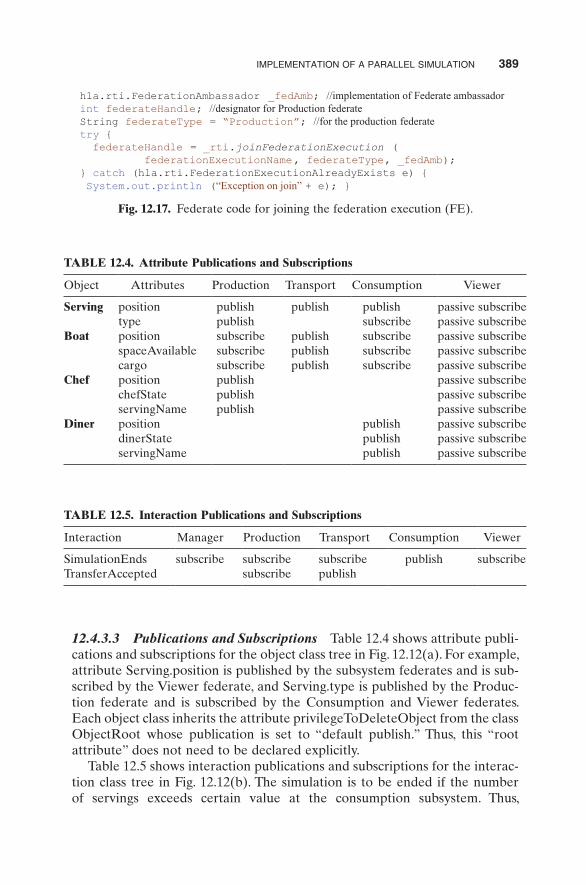
12.4.3.3 Publications and Subscriptions Table 12.4 shows attribute publi-cations and subscriptions for the object class tree in Fig. 12.12(a). For example, attribute Serving.position is published by the subsystem federates and is sub-scribed by the Viewer federate, and Serving.type is published by the Produc-tion federate and is subscribed by the Consumption and Viewer federates. Each object class inherits the attribute privilegeToDeleteObject from the class ObjectRoot whose publication is set to “default publish.” Thus, this “root attribute” does not need to be declared explicitly.

Table 12.5 shows interaction publications and subscriptions for the interac-tion class tree in Fig. 12.12(b). The simulation is to be ended if the number of servings exceeds certain value at the consumption subsystem. Thus,


SimulationEnds is published by the Consumption federate and subscribed by other federates. As another example, TransferAccepted is published by the Transport federate and subscribed by the Production federate.

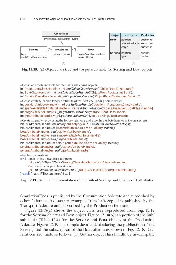
Figure 12.18(a) shows the object class tree reproduced from Fig. 12.12 for the Serving object and Boat object. Figure 12.18(b) is a portion of the pub/sub table (Table 12.4) for the Serving and Boat objects at the Production federate. Figure 12.19 is a sample Java code declaring the publication of the Serving and the subscription of the Boat attributes shown in Fig. 12.18. Dec-larations are made as follows: (1) Get an object class handle by invoking the

Fig. 12.19. Sample implementation of pub/sub of Serving and Boat object attributes.

//Get an object-class-handle for the Boat and Serving objects int RestaurantClassHandle = _rti.getObjectClassHandle(“ObjectRoot.Restaurant”); int BoatClassHandle = _rti.getObjectClassHandle(“ObjectRoot.Restaurant.Boat”); int ServingClassHandle = _rti.getObjectClassHandle(“ObjectRoot.Restaurant.Serving”);

//Get an attribute-handle for each attribute of the Boat and Serving object classes int positionAttributeHandle = _rti.getAttributeHandle(“position”, RestaurantClassHandle); int spaceAvailableAttributeHandle = _rti.getAttributeHandle(“spaceAvailable”, BoatClassHandle); int cargoAttributeHandle = _rti.getAttributeHandle(“cargo”, BoatClassHandle); int typeAttributeHandle = _rti.getAttributeHandle(“type”, ServingClassHandle);

//Create an empty set by using the factory reference and store the attribute handles in the created sets hla.rti.AttributeHandleSetFactory ahFactgory = RTI.attributeHandleSetFactory(); hla.rti.AttributeHandleSet boatAttributeHandles = ahFactory.create(); boatAttributeHandles.add(positionAttributeHandle); boatAttributeHandles.add(spaceAvailableAttributeHandle); boatAttributeHandles.add(cargoAttributeHandle); hla.rti.AttributeHandleSet servingAttributeHandles = ahFactory.create(); servingAttributeHandles.add(positionAttributeHandle); servingAttributeHandles.add(typeAttributeHandle);

//Declare publications try { //publish the object class attributes _rti.publishObjectClass (ServingClassHandle, servingAttributeHandles); //subscribe the object class attributes _rti.subscribeObjectClassAttributes (BoatClassHandle, boatAttributeHandles); } catch (hla.rti.RTIexception e) { … }

Fig. 12.18. (a) Object class tree and (b) pub/sub table for Serving and Boat objects.

Object Attributes Production

Boat

position spaceAvailable cargo

subscribe subscribe subscribe

Serving position type

publish publish

ObjectRoot

privilegeToDeleteObject : String

Restaurant

position: position

Boat

(b)(a)

spaceAvailable: boolean cargo : String

Serving

type: sushiTypeEnumeration


getObjectClassHandle () function; (2) get attribute handles by invoking the getAttributeHandle () method; (3) the attribute handles to be subscribed are stored in separate sets; and (4) the to-be-published or to-be-subscribed attri-butes are published or subscribed by invoking publishObjectClass () or sub-scribeObjectClassAttributes ().

12.4.4 Executing the Restaurant Federation

The overall procedure for preparing and executing your own federation was described earlier in Section 12.3.3 (See Fig. 12.10). In this section, we will show you how to download a sample implementation of the restaurant federation and run the program. More details may be found in the HLA Book [Kuhl et al. 2000]. Even if you do not sufficiently understand the internal workings of the sushi restaurant federation, you are advised to follow the steps explained below to get familiar with it.

12.4.4.1 Download and Installation Steps for downloading and installing the Sushi Restaurant Federation together with HLA/RTI software are as follows:

1. Download the restaurant federation sample code and HLA/RTI soft-ware from the following website: http://authors.phptr.com/kuhl.

2. Unzip the downloaded file into a directory named <kuhl>. The top-level directories in the directory <kuhl> are• <kuhl>\bin: class files for the implementation of restaurant

federation• <kuhl>\config: configuration data needed to run the restaurant

federation• <kuhl>\doc: all documents• <kuhl>\lib: Java archives needed to run RTI and the restaurant

federation• <kuhl>\src: Java source for the implementation of restaurant

federation3. Install a Java run-time environment by running jre-1_2_2_005-win.exe

located in the <kuhl> directory.

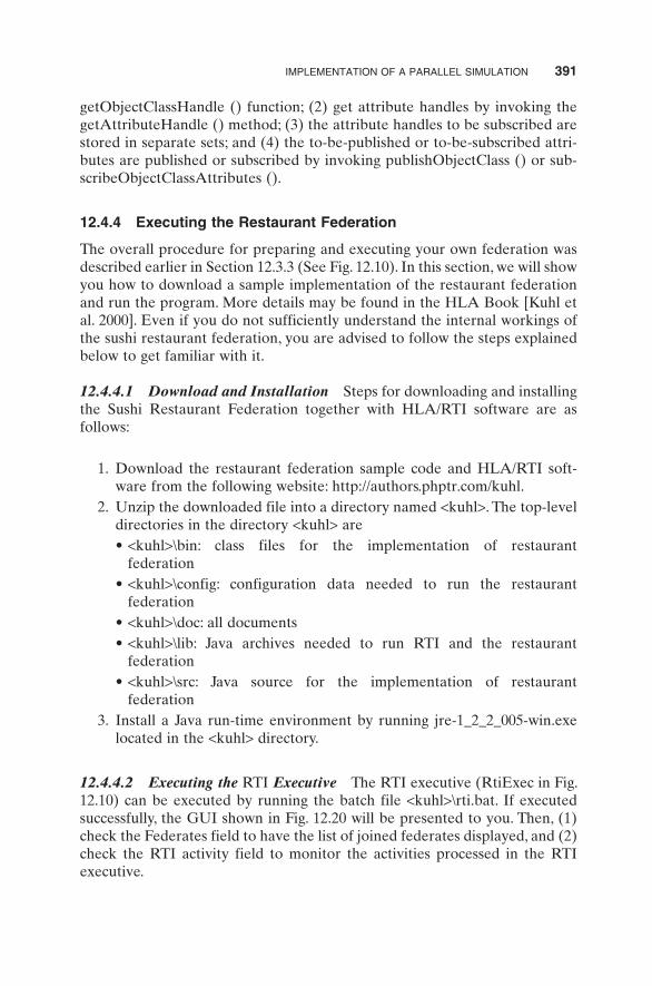
12.4.4.2 Executing the RTI Executive The RTI executive (RtiExec in Fig. 12.10) can be executed by running the batch file <kuhl>\rti.bat. If executed successfully, the GUI shown in Fig. 12.20 will be presented to you. Then, (1) check the Federates field to have the list of joined federates displayed, and (2) check the RTI activity field to monitor the activities processed in the RTI executive.


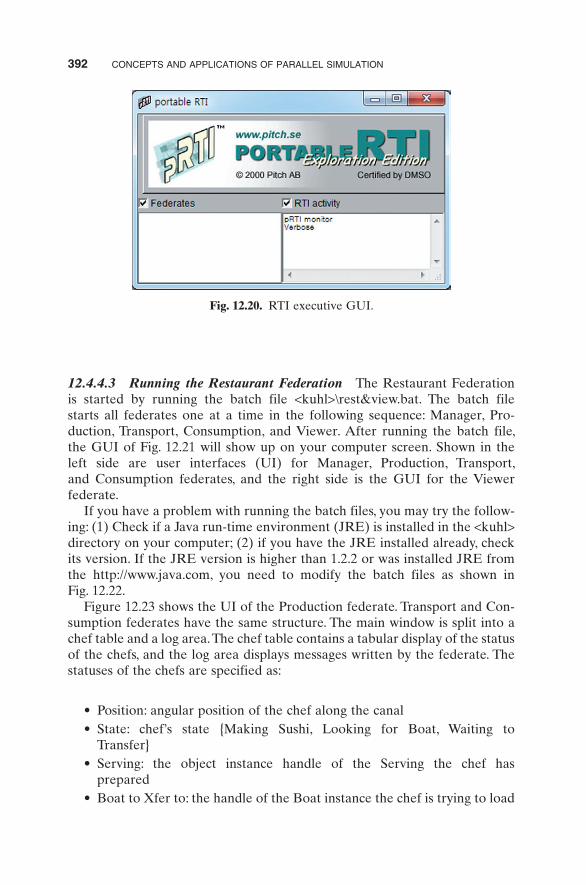
12.4.4.3 Running the Restaurant Federation The Restaurant Federation is started by running the batch file <kuhl>\rest&view.bat. The batch file starts all federates one at a time in the following sequence: Manager, Pro-duction, Transport, Consumption, and Viewer. After running the batch file, the GUI of Fig. 12.21 will show up on your computer screen. Shown in the left side are user interfaces (UI) for Manager, Production, Transport, and Consumption federates, and the right side is the GUI for the Viewer federate.

If you have a problem with running the batch files, you may try the follow-ing: (1) Check if a Java run-time environment (JRE) is installed in the <kuhl> directory on your computer; (2) if you have the JRE installed already, check its version. If the JRE version is higher than 1.2.2 or was installed JRE from the http://www.java.com, you need to modify the batch files as shown in Fig. 12.22.

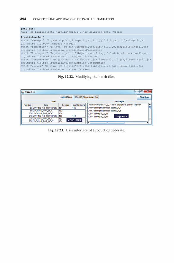
Figure 12.23 shows the UI of the Production federate. Transport and Con-sumption federates have the same structure. The main window is split into a chef table and a log area. The chef table contains a tabular display of the status of the chefs, and the log area displays messages written by the federate. The statuses of the chefs are specified as:

• Position: angular position of the chef along the canal• State: chef’s state {Making Sushi, Looking for Boat, Waiting to

Transfer}• Serving: the object instance handle of the Serving the chef has

prepared• Boat to Xfer to: the handle of the Boat instance the chef is trying to load

Fig. 12.20. RTI executive GUI.

Fig

. 12.

21.

Res

taur

ant

fede

rati

on e

xecu

tion

s G

UI.

393


Fig. 12.22. Modifying the batch files.

Fig. 12.23. User interface of Production federate.

modeling and simulation of discrete-event systems || concepts and applications of parallel...

Documents