modeling and control coordination of power systems with ...€¦ · the network active- or...
TRANSCRIPT

Modeling and Control Coordination of Power Systems with FACTS Devices in
Steady-State Operating Mode
by
Van Liem NGUYEN
Achieving International Excellence
This thesis is presented for the degree of Doctor of Philosophy of The University of Western Australia
Energy Systems Centre School of Electrical, Electronic and Computer Engineering
2008

______________________________________________________________________
(i)
ACKNOWLEDGEMENTS
I would like to express my sincere gratitude to my supervisor, Associate Professor T. T.
Nguyen, for providing me the opportunity to undertake this research, along with his
excellent guidance, constant support and invaluable encouragement throughout my PhD
candidature at The University of Western Australia.
I would like to thank the staff at the Energy Systems Centre for their assistance and the
use of the facilities of the Centre. Thanks are also extended to all the postgraduate
students studying at the Energy Systems Centre for their friendship, support and
encouragement.
I would like to express my boundless gratitude towards my parents, especially my
beloved Father who passed away during the course of my PhD study, my sisters and
brothers for their love and constant encouragement throughout my study. I would also
like to thank my wife, Kim Loan, for her love, patience, support and understanding
during every stage of my life and my work. Thanks also go to my loved children, Thanh
Luan and Ngoc Lam, who give me the motivation and objective to work and study. I
would like to dedicate the thesis to my family.
Finally, I would like to express my special appreciation to the scholarship granted by
the Government of Vietnam through Project 322, the Ad hoc scholarship awarded by
the Energy Systems Centre and SIRF Scholarship provided by The University of
Western Australia.

______________________________________________________________________
(ii)
ABSTRACT
This thesis is devoted to the development of new models for a recently-implemented
FACTS (flexible alternating current transmission system) device, the unified power
flow controller (UPFC), and the control coordination of power systems with FACTS
devices in steady-state operating mode. The key objectives of the research reported in
the thesis are, through online control coordination based on the models of power
systems having FACTS devices, those of maximising the network operational benefit
and restoring system static security following a disturbance or contingency.
Based on the novel concept of interpreting the updated voltage solutions at each
iteration in the Newton-Raphson (NR) power-flow analysis as dynamic variables, the
thesis first develops a procedure for representing the unified power flow controllers
(UPFCs) in the steady-state evaluation. Both the shunt converter and series converter
control systems of a UPFC are modeled in their dynamical form with the discrete time
variable replaced by the NR iterative step in the power-flow analysis. The key
advantage of the model developed is that of facilitating the process of UPFC constraint
resolution during the NR solution sequence. Any relative priority in control functions
pre-set in the UPFC controllers is automatically represented in the power-flow
formulation.
Although the developed UPFC model based on the dynamic simulation of series and
shunt converter controllers is flexible and general, the number of NR iterations required
for convergence can be large. Therefore, the model is suitable mainly for power system
planning and design studies. For online control coordination, the thesis develops the
second UPFC model based on nodal voltages. The model retains all of the flexibility
and generality of the dynamic simulation-based approach while the number of iterations
required for solution convergence is independent of the UPFC controller dynamic
responses.
Drawing on the constrained optimisation based on Newton’s method together with the
new UPFC model expressed in terms of nodal voltages, a systematic and general
method for determining optimal reference inputs to UPFCs in steady-state operation is

______________________________________________________________________
(iii)
developed. The method is directly applicable to UPFCs operation with a high-level line
optimisation control (LOC) for maximising the network operational benefit. By using a
new continuation technique with adaptive parameter, the algorithm for solving the
constrained optimisation problem extends substantially the region of convergence
achieved with the conventional Newton’s method.
Having established the foundation provided by the comprehensive models developed
for representing power systems with FACTS devices including the UPFC, the research,
in the second part, focuses on real-time control coordination of power system
controllers, with the main purpose of restoring power system static security following a
disturbance or contingency.
At present, as the cost of phasor measurement units (PMUs) and wide-area
communication network is on the decrease, the research proposes and develops a new
secondary voltage control where voltages at all of the load nodes are directly controlled,
using measured voltages. The new secondary voltage control avoids the possible
degradation of the performance of the existing coordinated secondary voltage control
which is based on the direct voltage control at only a limited number of load nodes. The
control strategy developed is fully adaptive to any changes in loads and/or system
configuration.
However, to achieve the lowest possible system operating cost, real-time corrective
control rather than preventative control is required. Depending on the nature of the
disturbance or contingency, secondary voltage control might not be able to provide the
necessary corrective control to restore power-flow security. In order to provide a
comprehensive control scheme which has the capability of restoring power system static
security in its entirety, the final research contribution made in the thesis is that of
developing a coordinated secondary control scheme for restoring voltage and/or power-
flow security subsequent to a disturbance/contingency, and, simultaneously, minimising
the network active- or reactive-power loss. The active- or reactive-power loss
minimisation leads to optimal reactive-power schedule for generators and compensators
together with system voltage profile while only a limited number of load nodes referred
to as the pilot nodes are selected for direct control. In addition to the voltage control
function, the new scheme includes FACTS devices of the series form or UPFC to

______________________________________________________________________
(iv)
achieve the corrective control for removing transmission circuit overloading. For
enhancing the accuracy in control and coordinating the time responses of the power
system primary controllers and secondary control, each secondary control cycle is
subdivided into a number of steps which is adaptive to the nature of the
disturbance/contingency.
State-of-the-art computer systems for implementing the comprehensive secondary
control law developed are referred to, and discussed in the thesis.

______________________________________________________________________
(v)
LIST OF PRINCIPAL SYMBOLS
SYMBOLS USED IN CHAPTER 2
V, I vectors of the nodal voltages and nodal currents respectively
|V|, θ vectors of the system voltage magnitudes and phase angles
respectively
u vector of the control variables
Y network nodal admittance matrix
f vector function associated with nonlinear power-flow equations
h vector function associated with operating limits of individual
power system elements
α delay angle
Xtcr effective reactance of TCR
XL reactance of the TCR reactor
|Vhsvc|, Vsvcref SVC high-voltage node voltage magnitude and its reference,
respectively
asvc SVC slope reactance
Isvc SVC current
Bsvc SVC susceptance
Bsvcmax, Bscvmin SVC susceptance maximum (capacitive) and minimum
(inductive) limit values respectively
Plsvc SVC low-voltage node active-power
XC TCSC capacitor reactance
Xbypass TCSC net reactance
Xtcr(α) variable inductive reactance
Xtcsc(α) TCSC effective reactance
αr resonant delay angle
αLlim, αClim TCSC delay angle limits in inductive region and capacitive
region respectively
XLlim, XClim TCSC inductive reactance and capacitive reactance limits
respectively

______________________________________________________________________
(vi)
Pline, Plinesp transmission line active-power flow and its specified value,
respectively
Xtcscmin, Xtcscmax TCSC minimum (capacitive) reactance and maximum (inductive)
reactance limits respectively
|Vhsta|, Vstaref STATCOM high-voltage node voltage magnitude and its
reference, respectively
asta STATCOM reactance slope
Ista STATCOM current
Istamax, Istamin STATCOM maximum and minimum current limits respectively
Plsta STATCOM low-voltage node active-power
SYMBOLS USED IN CHAPTER 3
VE, VB UPFC shunt converter and series converter voltage sources,
respectively
VK, VL, Vi voltage phasors at nodes K, L and i, respectively
|VB|, θB UPFC series converter voltage magnitude and phase angle,
respectively
|VK|, θK magnitude and phase angle of voltage phasor at node K
respectively
|VL|, θL magnitude and phase angle of voltage phasor at node L
respectively
IE, IB UPFC shunt converter and series converter currents, respectively,
at their AC terminals
ZE, ZB UPFC shunt converter and series converter coupling transformers
leakage impedances, respectively
YE, YB UPFC shunt converter and series converter coupling transformers
admittances, respectively
YKi element (K,i) of network nodal admittance matrix
PKsp, QKsp specified active- and reactive-power load demands at node K,
respectively
fPEB residual function associated with the net active-power exchange
between the UPFC and the network.

______________________________________________________________________
(vii)
fVupfc, fPupfc, fQupfc residual functions associated with the voltage control, active-
power control and reactive-power control, respectively, of the
UPFC of the UPFC
Vref, Pref, Qref UPFC reference values for the voltage magnitude, active-power
flow and reactive-power flow respectively
0BV , 0
Bθ initial value for the UPFC series voltage magnitude and phase
angle, respectively
0EV , 0
Eθ initial value for the UPFC shunt voltage magnitude and phase
angle, respectively
0KV , 0
LV initial value for voltage magnitudes at nodes K and L,
respectively
XB, XE UPFC series converter and shunt converter coupling transformers
inductive reactance respectively
|YB|, αB UPFC series converter coupling transformer admittance module
and angle, respectively
PKinj, QKinj total active- and reactive-power injections of the UPFC at node K
PKM0, QKM0 active- and reactive-power flows in the transmission line between
nodes K and M after the removal of the UPFC series voltage
source
PMinj, QMinj active- and reactive-power injections of the UPFC at node M
ZKM impedance of the transmission line between node K and M
QKMinj reactive-power which combines with QKM0 to give the total
transmission line reactive-power flow at node K
QKKinj reactive-power injection from the UPFC shunt converter
operation related to the voltage control function at node K
f objective function
SYMBOLS USED IN CHAPTER 4
Vref, Pref , Qref UPFC voltage, active-power and reactive-power references,
respectively
t time variable
VK(t) voltage phasor at node K at t

______________________________________________________________________
(viii)
reference for voltage magnitude at node K
IE(t) shunt converter current phasor at t
Vdc(t), Vdcref DC voltage at t and its reference value
IEp(t), IEq(t) in-phase and quadrature components, respectively, of the UPFC
shunt converter current at t with respect to the reference given by
VK(t)
IEpref(t), IEqref(t) in-phase and quadrature components, respectively, of required
shunt converter current at t
VEp(t), VEq(t) in-phase and quadrature components, respectively, of the shunt
converter voltage source at t
|VE(t)|, θE(t) magnitude and phase angle, respectively, of the shunt converter
voltage source at t
θK(t) phase angle of voltage phasor VK(t)
VL(t), VK(t) voltage phasors of nodes L and K, respectively, at t
IB(t) UPFC series converter current phasor at t
VBp(t), VBq(t) in-phase and quadrature components of the UPFC series
converter voltage at t
|VB(t)|, θB(t) magnitude and phase angle, respectively, of the UPFC series
converter voltage at t
J Jacobian matrix
f vector of residual functions.
p Newton-Raphson iterative step
VK(p), VL(p) voltage phasors of node K and L, respectively, at step p
VB(p), IB(p) UPFC series converter voltage and current phasor, respectively,
at step p
θK(p) phase angle of the voltage phasor of node K at step p
IBp(p), IBq(p) in-phase and quadrature components, respectively, of the UPFC
series converter current phasor with respect to the reference given
by VK(p) at step p
IBpref(p), IBqref(p) in-phase and quadrature components, respectively, of the required
UPFC series converter current phasor at step p
∆IBp(p), ∆IBq(p) differences between the in-phase and quadrature components of
the UPFC series converter current phasor and their required
values, respectively, at step p

______________________________________________________________________
(ix)
PB(p) active-power exchange between the UPFC shunt and series
converters at step p
∆VK(p) difference between the voltage magnitude of node K and its
reference value at step p
VBp(p+1), VBq(p+1) in-phase and quadrature components of the UPFC series converter
voltage phasor at step p+1
|VB(p+1)|, θB(p+1) magnitude and phase angle, respectively, of the UPFC series
converter voltage phasor at step p+1
phase angle of the series converter voltage phasor at step p+1
|VB(p+1)|, θB(p+1) magnitude and phase angle, respectively, of the UPFC series
converter voltage at step p+1
IEp(p+1), IEq(p+1) in-phase and quadrature components of the UPFC shunt
converter current phasor at step p+1
IE(p+1), ψE(p+1) magnitude and phase angle, respectively, of the UPFC shunt
converter current at step p+1
XB UPFC series converter transformer reactance
K1, K2, K3 coefficients derived from the UPFC controller gains
VBmax maximum allowable limit of the UPFC series converter voltage
magnitude
VLmin, VLmax minimum and maximum allowable limits of the UPFC line side
voltage magnitude respectively
PBmax maximum allowable limit of active-power exchange between the
UPFC shunt and series converters
IBmax maximum allowable limit of the UPFC series converter current
IEmax maximum allowable limit of the UPFC shunt converter current
k Newton-Raphson iterative step in the range where the second
level of control is active
Pline active-power flow in the transmission line controlled by UPFC
SYMBOLS USED IN CHAPTER 5
VF, |VF|, θF voltage phasor, its magnitude and phase angle, respectively, at
node F

______________________________________________________________________
(x)
IEp, IEq active-power and reactive-power components of the UPFC shunt
converter current, respectively
PKsp, QKsp specified active- and reactive-power at node K respectively
Xs slope reactance
QShref UPFC high-voltage side node reactive-power reference
αref reference value for the UPFC phase shift between the line side
voltage VL and busbar voltage VK
VBref, θBref series voltage magnitude and phase angle reference signal inputs
to the UPFC
VLref reference value for the UPFC line-side voltage reference
Zref UPFC series impedance reference
PE, PEmax active-power flow in the DC link and its maximum limit,
respectively
SYMBOLS USED IN CHAPTER 6
Vref, Vrefopt desirable and optimal values, respectively, of the UPFC voltage
reference
QShref, QShrefopt desirable and optimal values, respectively, of the UPFC high-
voltage side node reactive-power reference
Pref, Prefopt desirable and optimal values, respectively, of the UPFC active-
power reference
Qref, Qrefopt desirable and optimal values, respectively, of the UPFC reactive-
power reference
VLref, VLrefopt desirable and optimal values, respectively, of the UPFC line-side
voltage reference
αref, αrefopt desirable and optimal values, respectively, of UPFC phase shift
reference;
VBref, VBrefopt desirable and optimal values, respectively, of the UPFC series
voltage magnitude reference
θBref, θBrefopt desirable and optimal values, respectively, of the UPFC series
voltage angle reference
Zref, Zrefopt desirable and optimal values, respectively, of the UPFC series
impedance reference

______________________________________________________________________
(xi)
xi , Xrefi the ith elements of vector x and refX , respectively
Wi weighting factor associated with xi
Sk, Sspk apparent power flow in transmission line k at either sending- or
receiving end, and the specified value to which power flow Sk is
to be controlled
|Vl|, Vspl voltage magnitude at node l and its target specified value,
respectively
kSW , lVW weighting factors associated with Sk and Vl, respectively, which
reflect the relative priority in control assigned to the individual
controlled quantities
Sks, Skr apparent power flows at the sending- and receiving-end of
transmission line k, respectively
ZL, YL series impedance and shunt admittance of the transmission line
equivalent π circuit
λ , µ Lagrange-multiplier vectors associated with F and G+,
respectively
+G vector of functions relating to inequality constraints
pz solution for vector z at the pth iteration in the Newton solution
sequence
WV, WP, WQ weighting factors associated with voltage, active- and reactive-
power flow controls, respectively
|VC |, PC, QC voltage magnitude at node C, active- and reactive-power flows on
transmission line SC at node C
SYMBOLS USED IN CHAPTER 7
|Vpl|, Vplsp, Vn measured, set-point and nominal values, respectively, of the
voltage magnitude at the pilot node
Qgeni, Qgenspi measured and set-point values, respectively, of reactive-power of
generator i
|Vgeni|, Vrefgeni measured and reference values, respectively, of the voltage
magnitude of generator i

______________________________________________________________________
(xii)
∆Vrefgeni variation of the voltage magnitude reference of generator i
Iexi exciter current of generator i
N control signal
α, β integral and proportional gains, respectively, of the secondary
voltage control
'plV measured value obtained by digital filtering based on three
successive samples of |Vpl|
Qr participation factor
Qn nominal reactive-power of the controlling generator
Vplsp vector of the set-point voltage magnitudes at the pilot nodes
Qgensp vector of the set-point reactive-power of the controlling
generators
V0refgen vector of the pre-specified voltage references for the controlling
generators
|Vplk| measured voltage magnitude at pilot node k
|Vgeni|, Vrefgeni measured and reference values, respectively, of the voltage
magnitude of controlling generator i
Qgeni measured reactive-power of controlling generator i
Iexi exciter current of generator i
npl number of pilot nodes
ngen number of controlling generators
αC control gain of the coordinated secondary voltage control
p, (p+1) current step and next step, respectively, of the control procedure
Notation ||.|| norm of a vector
pplV vector of the measured voltage magnitudes at the pilot nodes
pgenQ vector of the measured reactive-power of the controlling
generators
V0refgen vector of the pre-specified voltage references for the controlling
generators
prefgenV vector of the current voltage references for the controlling
generators
1+∆ prefgenV required voltage reference variation of the controlling generators

______________________________________________________________________
(xiii)
CVpl sensitivity matrix associated with voltage variations at pilot nodes
to the voltage reference variations of the controlling generators
CQ sensitivity matrix associated with the generator reactive-power
variation to the voltage reference variations of the controlling
generators
λV , λQ , λU weighting factors associated with the pilot node voltages,
controlling generator reactive-powers and controlling generator
terminal voltage references, respectively
∆Vgenmax vector of the maximum allowable variations of the controlling
generator voltage magnitudes
Vplmin,Vplmax vectors of the minimum and maximum allowable voltages at pilot
nodes
Vsenmin, Vsenmax vectors of the minimum and maximum allowable voltage
magnitudes at the sensitive nodes
Vhgenmin, Vhgenmax vectors of the minimum and maximum allowable voltage
magnitudes at the high voltage side of the controlling generators
psenV vector of the measured voltage magnitudes at the sensitive nodes
phgenV vector of the measured voltage magnitudes at the high-voltage
sides of controlling generators
CVsen sensitivity matrix associated with voltage variation at the sensitive
nodes to the voltage reference variations of the controlling
generators
Chgen sensitivity matrix associated with voltage variation at the high
voltage side nodes of the controlling generators to the voltage
reference variations of the controlling generators
a, b and c diagonal matrices the diagonal elements of which are coefficients
of the straight lines representing operating diagrams for the
controlling generators (P,Q,V)
EDij electrical distance between nodes i and j
i
i
Q
V
∂∂
, j
j
Q
V
∂
∂ sensitivities of the voltage magnitude change at nodes i and j to
their injected reactive-power change, respectively

______________________________________________________________________
(xiv)
i
j
Q
V
∂
∂ sensitivity of the voltage magnitude change at node j to the
injected reactive-power change at node i
j
i
Q
V
∂∂
sensitivity of the voltage magnitude change at node i to the
injected reactive-power change at node j
SYMBOLS USED IN CHAPTER 8
Pload, Qload vectors of the load node active- and reactive-power, respectively
∆Pload, ∆Qload vectors of the active- and reactive-power variations at load nodes
∆|V| vector of the changes in nodal voltage magnitudes including that
of the slack node
∆θ vector of the changes in nodal voltage phase angles excluding that
of the slack node which is chosen as the phase angle reference
Pgen vector of the generator active-power
∆Pgen vector of the generator active-power variations
|Vgen| vector of the voltage magnitudes at the generator terminals
∆|Vgen| vector of the changes in voltage magnitudes at the generator
terminals
∆Vgenref vector of the changes in the reference inputs to the excitation
controllers
Plsvc vector of nodal active-power at the nodes on the low voltage sides
of the SVC coupling transformers
∆Plsvc vector of the active-power variation at the nodes on the low
voltage sides of the SVC coupling transformers
|Vhsvc| vector of the voltage magnitudes at the nodes on the high voltage
sides of the SVC coupling transformers
asvc diagonal matrix the elements of which are reactance slopes of
SVCs
Isvc vector of SVC currents
Vsvcref vector of the SVC voltage references
∆Vsvcref vector of the changes in the SVC voltage references
Plsta vector of nodal active-power at the low voltage side nodes of the

______________________________________________________________________
(xv)
STATCOM coupling transformers
|Vhsta| vector of voltage magnitudes at high voltage side nodes of the
STATCOM coupling transformers
asta diagonal matrix the elements of which are reactance slopes of
STATCOMs
Ista vector of STATCOM currents
∆Vstaref vector of the changes in the STATCOM voltage references
Vslref reference value for the slack node voltage magnitude
nnode number of the power system nodes
nsvc number of SVCs
nsta number of STATCOMs
ngen number of generators
A system sensitivity matrix
∆|VL| vector of the changes in the load nodes voltage magnitudes
∆|VC| vector of the changes in the voltage magnitudes of the slack node,
generator nodes, low-voltage side nodes of SVCs and
STATCOMs
Cv system voltage sensitivity matrix which gives the linear relation
between the system voltage variation and the changes in
controllers references
CvL, CvC submatrices of matrix Cv associated with ∆|VL| and ∆|VC|,
respectively
Qgen vector of the generator reactive-powers
Vtarget vector of the specified target voltage magnitudes at the load
nodes
ε vector of the differences between the specified target values and
the current values of voltage magnitudes at the load nodes
∆VCmin, ∆VCmax vectors of the deviations between the current operating voltage
magnitudes and the allowable minimum and maximum voltage
magnitudes of the slack node, generator nodes, low-voltage nodes
of SVCs and STATCOMs
∆Qgenmin, ∆Qgenmax vectors of the differences between the minimum and maximum
reactive-power limits of generators, respectively, and their current
operating reactive-powers

______________________________________________________________________
(xvi)
∆Bsvcmin, ∆Bsvcmax vectors of the differences between the inductive limits and
capacitive limits of SVCs, respectively, and their current
operating susceptances
∆Istamin, ∆Istamax vectors of the differences between the minimum and maximum
current limits of STATCOMs, respectively, and their operating
currents
0refV vector of the current controllers reference settings
Vref vector of optimal reference settings for the controllers
SYMBOLS USED IN CHAPTER 9
ntcsc number of TCSCs
Xtcsc, Xtcscref TCSC reactance and its reference value, respectively
stcsc, rtcsc TCSC sending-end and receiving-end node nodes, respectively
Ystcsc,i element (stcsc,i) of the nodal admittance matrix of the power
system excluding the TCSC
Yrtcsc,i element (rtcsc,i) of the nodal admittance matrix of the power
system excluding the TCSC
Vstcsc , Vrtcsc nodal voltages at nodes stcsc and rtcsc, respectively
Xtcsc0 TCSC reactance at the current operating condition
Xtcscmin, Xtcscmax minimum (capacitive) and maximum (inductive) allowable
values, respectively, of the TCSC reactance
∆Xtcsc TCSC reactance variation
∆Xtcscmin, ∆Xtcscmax differences between the TCSC minimum and maximum reactance
limits, respectively, and the TCSC reactance at the current
operating condition
∆Xtcsc vector of the changes in TCSC reactances
∆Xtcscref vector of the changes in TCSC reactances references
I unit matrix
Ptcsc, Qtcsc vectors of the nodal active- and reactive-power at nodes stcsc’s of
all TCSCs, respectively
∆Xtcscmin, ∆Xtcscmax vectors of the differences between the minimum and maximum
reactance limits of TCSCs and their reactance at the current
operating condition, respectively
______________________________________________________________________
(xvii)
∆Rref vector of the changes in the reference input signals to controllers
SS, SR apparent power flows at the sending-end and receiving-end
nodes, respectively
PS, QS active- and reactive-power flows at the sending-end node of the
branch
PR, QR active- and reactive-power flows at the receiving-end node of the
branch
∆Vmin, ∆Vmax vector of deviations between the allowable minimum and
minimum values and the current operating values of system
voltage magnitudes, respectively
∆Xtcscmin, ∆Xtcscmax vectors of the differences between the minimum and maximum
reactance limits of TCSCs (they are dynamic limits depending on
the TCSC operating condition), respectively, and their current
operating reactance
∆Sbmax vector of the differences between the maximum power flow limits
of all branches and their current operating apparent power flow
SYMBOLS USED IN CHAPTER 10
nupfc number of UPFCs
nltc number of LTC transformers
Rupfcref vector of UPFC reference settings for controlled quantities
fC, fR, h vector functions in the UPFC steady-state model associated with
circuit constraints, control functions and operating limits
Vupfcref reference setting for the voltage magnitude
Pupfcref, Qupfcref reference settings for the active- and reactive-power flows
∆Rupfcref vector of the changes in UPFC reference input settings
h0 value of vector h at the current operating point
Pgensp, Vgensp scheduled active-power generation of the generator and the
specified voltage magnitude at the generator terminal,
respectively
PHsp, QHsp specified active- and reactive-power demands at the high-voltage
side node of the transformer, respectively

______________________________________________________________________
(xviii)
|VG|, |VH| voltage magnitudes at the low- and high-voltage side nodes of the
transformer, respectively
Vltcref reference value of the voltage magnitude at the high-voltage side
node of the transformer
PH, QH nodal active- and reactive-power at the high-voltage side node of
the transformer, respectively
T LTC transformer per-unit voltage ratio
Tmin, Tmax minimum and maximum values, respectively, of the LTC
transformer voltage ratio
∆Tltc vector of the changes in LTC transformer voltage ratios
∆Rref vector of the changes in reference input signals to controllers,
which can include generators, SVCs, STATCOMs, TCSCs,
UPFCs and LTC transformers.
∆Vltcref vector of the changes in the LTC transformer voltage references
∆Vupfcref vector of the changes in the UPFC voltage
∆Pupfcref, ∆Qupfcref vectors of the changes in the UPFC active- and reactive-power
references, respectively.
∆Rref1 vector of the changes in reference input signals to the subset of
controllers, which participate in the secondary control
∆|V|1, ∆θ1 vectors of the changes in voltage magnitudes and phase angles at
the pilot nodes, important nodes together with those at other
nodes, which are needed for forming the changes in circuit power
flows, controller operating quantities and objective function
∆Tltc1, ∆Xtcsc1 vectors of the changes in LTC transformers voltage ratios and
TCSCs reactances, respectively, which participate in the
secondary control
Qgen, Qsl, Qcom total reactive-powers generated from generators, slack node and
compensators, respectively
Qload total reactive-power consumed by loads
Qloss, Qgain total reactive-power loss in the series reactances and the total
reactive-power gain from shunt-path capacitances of transmission
circuits, respectively
α diagonal matrix of the control gains

______________________________________________________________________
(xix)
Cvpl matrix partition of Cv associated with the pilot nodes, which gives
the sensitivity of the pilot node voltage magnitudes with the
control variables
Vplspi set point value for the voltage magnitude of pilot node i
|| 0pliV initial value for the voltage magnitude of pilot node i immediately
after a contingency/disturbance
|Vpli| measured value for the voltage magnitude of pilot node i in
response to secondary control
CL sensitivity matrix associated with constrained quantities
CS submatrix of the sensitivity matrix CL associated with the power
flows in the critical transmission circuits
S0, Smax vectors of the current circuit loadings in the critical transmission
circuits and their maximum allowable limits, respectively
βmax, βmin upper and lower allowable limits of the changes in apparent
power flow, respectively
CH matrix partition of CL associated with controller operating
quantities, which gives their sensitivities with the control
variables
H0, Hmin, Hmax vectors of the current values for controller operating quantities,
their minimum and maximum values, respectively
Rref10 vector of the current reference settings for controllers
Rref1min, Rref1max vectors of the minimum and maximum allowable values for
controllers reference setting, respectively.

______________________________________________________________________
(xx)
GLOSSARY
AC Alternating Current
AVR Automatic Voltage Regulator
CSVR Coordinated Secondary Voltage Control
DAS Data Acquisition System
DC Direct Current
DFT Discrete-Fourier Transform
EMS Energy Management System
FACTS Flexible Alternating Current Transmission System
FLOPS Floating Point Operations per Second
GTO Gate Turn-Off (thyristor)
IGBT Insulated Gate Bi-polar Transistor
KKT Karush-Kuhn-Tucker (condition)
LOC Line Optimisation Control
LP Linear Programming
LTC Load-Tap-Changing (transformer)
MIPS Million Instructions per Second
NR Newton-Raphson
OPF Optimal Power Flow
PI Proportional-Integral (controller)
PIM Power Injection Model
PMU Phasor Measurement Unit
PVR Primary Voltage Control
PWM Pulse-Width Modulation
SSSC Static Synchronous Series Compensator
STATCOM Static Synchronous Compensator
SVC Static VAr Compensator
SVR Secondary Voltage Control
TCR Thyristor Controlled Reactor
TCSC Thyristor Controlled Series Capacitor
TNA Transient Network Analyser
TSC Thyristor Switched Capacitor

______________________________________________________________________
(xxi)
TVR Tertiary Voltage Control
UPFC Unified Power Flow Controller
VSC Voltage Source Converter
WAMS Wide-Area Measurement System

______________________________________________________________________
(xxii)
TABLE OF CONTENTS
Chapter 1 Introduction ............................................................................................... 1
1.1 BACKGROUND AND SCOPE OF THE RESEARCH .................................... 1
1.2 OBJECTIVES .................................................................................................... 3
1.3 OUTLINE OF THE THESIS ............................................................................. 4
1.4 CONTRIBUTIONS OF THE THESIS .............................................................. 6
Chapter 2 Review of Steady-State Models of Power System Elements .................. 8
2.1 INTRODUCTION .............................................................................................. 8
2.2 NODAL FORMULATION OF POWER SYSTEM MODEL ........................... 9
2.3 FACTS DEVICES MODELS .......................................................................... 11
2.3.1 Modeling principle .................................................................................... 12
2.3.2 Static VAr compensator (SVC) ................................................................. 12
2.3.3 Thyristor controlled series capacitor (TCSC) ........................................... 17
2.3.4 Static synchronous compensator (STATCOM) ........................................ 24
2.4 FACTS DEVICE CONTROLLER .................................................................. 28
2.4.1 General ...................................................................................................... 28
2.4.2 FACTS controller input signal derivation ................................................. 29
2.4.3 Application of the dq0 transformation for phasor calculation .................. 30
2.5 SYSTEM MODEL ........................................................................................... 32
2.6 CONCLUSION ................................................................................................ 33
Chapter 3 Review of Steady-State Models of UPFC .............................................. 34
3.1 INTRODUCTION ............................................................................................ 34
3.2 UPFC STRUCTURE AND OPERATING PRINCIPLES ............................... 35
3.3 POWER LOSSES IN UPFC OPERATING CONDITION ............................. 37
3.4 UPFC CONTROL MODES AND OPERATING LIMITS ............................. 39
3.4.1 Shunt Converter ........................................................................................ 39
3.4.2 Series Converter ........................................................................................ 40

______________________________________________________________________
(xxiii)
3.4.3 Stand alone shunt and series compensation .............................................. 42
3.4.4 Operating limits ......................................................................................... 42
3.5 DECOUPLED UPFC MODEL ........................................................................ 43
3.6 TWO-VOLTAGE SOURCE MODEL ............................................................. 45
3.7 POWER INJECTION MODEL ....................................................................... 51
3.8 IDEAL TRANSFORMER UPFC MODEL ..................................................... 58
3.9 CONCLUSIONS .............................................................................................. 59
Chapter 4 Dynamic Simulation-Based UPFC Steady-State Model ...................... 60
4.1 INTRODUCTION ............................................................................................ 60
4.2 UPFC DYNAMICAL MODEL ....................................................................... 61
4.3 UPFC DYNAMICAL REPRESENTATION
IN POWER-FLOW ANALYSIS………………………………….………...66
4.3.1 Principle .................................................................................................... 66
4.3.2 Implementation for Power-flow Analysis ................................................. 66
4.4 SERIES VOLTAGE SOURCE ........................................................................ 71
4.4.1 Definitions ................................................................................................. 73
4.4.2 Transfer Function Simulation ................................................................... 73
4.5 SHUNT CURRENT SOURCE ........................................................................ 73
4.5.1 Definition .................................................................................................. 73
4.5.2 Transfer Function Simulation ................................................................... 73
4.6 UPFC SECOND LEVEL CONTROL ............................................................. 74
4.7 SIMULATION RESULTS ............................................................................... 77
4.7.1 System Configuration ............................................................................... 77
4.7.2 Case Study 1 .............................................................................................. 77
4.7.3 Case Study 2 .............................................................................................. 80
4.7.4 Case Study 3 .............................................................................................. 85
4.8 CONCLUSION ................................................................................................ 90

______________________________________________________________________
(xxiv)
Chapter 5 Nodal-Voltage Model of UPFC .............................................................. 92
5.1 INTRODUCTION ............................................................................................ 92
5.2 NEW UPFC MODEL DEVELOPMENT PRINCIPLES ................................. 93
5.3 UPFC NEW MODEL EQUATIONS ............................................................... 96
5.3.1 Circuit Constraints .................................................................................... 96
5.3.2 Interaction between the Shunt Converter and Series Converter ............... 97
5.3.3 Control Function Equations ...................................................................... 97
5.3.4 Discussion ............................................................................................... 101
5.4 UPFC INEQUALITY CONSTRAINTS ........................................................ 103
5.4.1 General .................................................................................................... 103
5.4.2 Shunt Converter Current Limit ............................................................... 103
5.4.3 Active-Power Exchange Limit ................................................................ 104
5.4.4 Series Injected Voltage Limit.................................................................. 105
5.4.5 Series Converter Current Limit ............................................................... 105
5.4.6 Line-side Voltage Limit .......................................................................... 106
5.5 COMPARISON BETWEEN THE NEW UPFC MODEL
AND OTHER ONES………………………………………………………106
5.5.1 Two-Voltage Source Model .................................................................... 106
5.5.2 Power Injection Model ............................................................................ 107
5.6 CONCLUSIONS ............................................................................................ 107
Chapter 6 Application of Nodal-Voltage UPFC Model for LOC ....................... 109
6.1 INTRODUCTION .......................................................................................... 109
6.2 POWER-FLOW ANALYSIS FORMULATION WITH UPFC MODEL
COMBINED WITH LOC ............................................................................ 110
6.2.1 Principal Concepts .................................................................................. 110
6.2.2 OPF Formulation with Specified UPFC References ............................... 113
6.2.3 OPF Formulation without Pre-specification of UPFCs References ........ 114
6.3 SOLUTION PROCEDURE BY NEWTON’S METHOD ............................. 118

______________________________________________________________________
(xxv)
6.4 APPLICATION OF THE CONTINUATION METHOD ............................. 122
6.4.1 General Concept ...................................................................................... 122
6.4.2 Adaptive Scheme .................................................................................... 122
6.5 CASE STUDY 4 ............................................................................................ 126
6.5.1 Power System Description ...................................................................... 126
6.5.2 Performance Study with Series Compensation ....................................... 127
6.5.3 UPFC Application Studies ...................................................................... 128
6.6 CONCLUSIONS ............................................................................................ 130
Chapter 7 Review of Secondary Voltage Control in Transmission Network .... 131
7.1 INTRODUCTION .......................................................................................... 131
7.2 VOLTAGE CONTROL REQUIREMENTS ................................................. 132
7.3 HIERARCHICAL VOLTAGE CONTROL STRUCTURE .......................... 133
7.3.1 General .................................................................................................... 133
7.3.2 Primary voltage control ........................................................................... 134
7.3.3 Secondary voltage control ....................................................................... 135
7.3.4 Tertiary voltage control ........................................................................... 136
7.4 SECONDARY VOLTAGE CONTROL SCHEMES .................................... 137
7.4.1 Former Secondary Voltage Control ........................................................ 137
7.4.2 Coordinated Secondary Voltage Control (CSVR) .................................. 142
7.5 PILOT NODE SELECTION .......................................................................... 151
7.5.1 General .................................................................................................... 151
7.5.2 Simple rule .............................................................................................. 152
7.5.3 Combined electrical distance and typology analysis .............................. 153
7.5.4 Optimisation-based selection using linearised network model ............... 154
7.5.5 Optimisation-based selection using nonlinear network model ............... 155
7.6 CONCLUSION .............................................................................................. 155

______________________________________________________________________
(xxvi)
Chapter 8 Application of Wide-Area Network of Phasor Measurements for
Secondary Voltage Control in Power Systems with FACTS Controllers .............. 157
8.1 INTRODUCTION .......................................................................................... 157
8.2 MODELING PRINCIPLES FOR SECONDARY VOLTAGE CONTROL . 159
8.3 SENSITIVITY MATRIX OF POWER SYSTEM ......................................... 160
8.3.1 Load......................................................................................................... 160
8.3.2 Generator ................................................................................................. 162
8.3.3 SVC ......................................................................................................... 163
8.3.4 STATCOM .............................................................................................. 164
8.3.5 Slack Node .............................................................................................. 165
8.3.6 System Sensitivity Matrix ....................................................................... 166
8.3.7 Discussion ............................................................................................... 169
8.3.8 Controller Sensitivity Matrices ............................................................... 169
8.4 CONTROL STRATEGY ............................................................................... 171
8.5 SECONDARY VOLTAGE CONTROL LOOP ............................................ 174
8.6 SIMULATION RESULTS ............................................................................. 175
8.6.1 Case Study 5 ............................................................................................ 177
8.7 CONCLUSIONS ............................................................................................ 180
Chapter 9 Secondary Control for Restoring Power System Security ................ 182
9.1 INTRODUCTION .......................................................................................... 182
9.2 LINEARISED MODEL OF TCSC .............................................................. 185
9.2.1 General .................................................................................................... 185
9.2.2 Linearised TCSC Model ......................................................................... 185
9.3 SENSITIVITY MATRIX OF POWER SYSTEM ......................................... 188
9.4 ACTIVE-POWER LOSS OBJECTIVE FUNCTION .................................... 191
9.5 TRANSMISSION LINE POWER FLOW ..................................................... 192
9.6 CONTROL STRATEGY ............................................................................... 194
9.7 MULTI-STEP SECONDARY CONTROL ................................................... 195

______________________________________________________________________
(xxvii)
9.8 SECONDARY CONTROL LOOP ................................................................ 197
9.9 SIMULATION RESULTS ............................................................................. 197
9.9.1 System Configuration ............................................................................. 197
9.9.2 Case Study 6 ............................................................................................ 199
9.10 CONCLUSIONS ............................................................................................ 203
Chapter 10 Robust Pilot-node Based Secondary Control Scheme for Security
Restoration in Restructured Power Systems ............................................................ 205
10.1 INTRODUCTION .......................................................................................... 205
10.2 LINEARISED UPFC MODEL FOR SECONDARY CONTROL ................ 207
10.3 LINEARISED MODEL FOR GENERATOR TRANSFORMER ................. 209
10.4 LINEARISED MODEL OF POWER SYSTEM ........................................... 212
10.4.1 Sensitivity Matrix for Dependent Variables ........................................... 212
10.4.2 Sensitivity Matrix for Constrained Quantities ........................................ 214
10.5 CHOICE OF OBJECTIVE FUNCTION IN SECONDARY CONTROL ..... 215
10.6 SECONDARY CONTROL STRATEGY ...................................................... 218
10.7 COMPUTER SYSTEMS FOR SECONDARY CONTROL ......................... 225
10.8 TIME COORDINATION BETWEEN PRIMARY CONTROLLERS AND
SECONDARY CONTROL RESPONSES ................................................... 226
10.9 SECONDARY CONTROL LOOP ................................................................ 227
10.10 REPRESENTATIVE STUDIES .................................................................... 229
10.10.1 Power System Description .................................................................. 229
10.10.2 Case Study 7: Load Demand Change .................................................. 230
10.10.3 Case Study 8: Transmission Line Outage ........................................... 233
10.11 CONCLUSIONS ............................................................................................ 238
Chapter 11 Conclusions and Future Work ............................................................. 240
11.1 CONCLUSIONS ............................................................................................ 240
11.2 FUTURE WORK ........................................................................................... 242
11.2.1 Real-time implementation of the new secondary control ....................... 243

______________________________________________________________________
(xxviii)
11.2.2 Priority for power-flow control in secondary control ............................. 243
11.2.3 Control coordination for power system stability improvements ............. 243
Bibliography………...………………………………………………………………..244
Appendices…….……………………………………………………………………..253

Modeling and Control Coordination of Power Systems with FACTS Devices in
Steady-State Operating Mode
by
Van Liem NGUYEN
Achieving International Excellence
This thesis is presented for the degree of Doctor of Philosophy of The University of Western Australia
Energy Systems Centre School of Electrical, Electronic and Computer Engineering
2008

______________________________________________________________________
(i)
ACKNOWLEDGEMENTS
I would like to express my sincere gratitude to my supervisor, Associate Professor T. T.
Nguyen, for providing me the opportunity to undertake this research, along with his
excellent guidance, constant support and invaluable encouragement throughout my PhD
candidature at The University of Western Australia.
I would like to thank the staff at the Energy Systems Centre for their assistance and the
use of the facilities of the Centre. Thanks are also extended to all the postgraduate
students studying at the Energy Systems Centre for their friendship, support and
encouragement.
I would like to express my boundless gratitude towards my parents, especially my
beloved Father who passed away during the course of my PhD study, my sisters and
brothers for their love and constant encouragement throughout my study. I would also
like to thank my wife, Kim Loan, for her love, patience, support and understanding
during every stage of my life and my work. Thanks also go to my loved children, Thanh
Luan and Ngoc Lam, who give me the motivation and objective to work and study. I
would like to dedicate the thesis to my family.
Finally, I would like to express my special appreciation to the scholarship granted by
the Government of Vietnam through Project 322, the Ad hoc scholarship awarded by
the Energy Systems Centre and SIRF Scholarship provided by The University of
Western Australia.

______________________________________________________________________
(ii)
ABSTRACT
This thesis is devoted to the development of new models for a recently-implemented
FACTS (flexible alternating current transmission system) device, the unified power
flow controller (UPFC), and the control coordination of power systems with FACTS
devices in steady-state operating mode. The key objectives of the research reported in
the thesis are, through online control coordination based on the models of power
systems having FACTS devices, those of maximising the network operational benefit
and restoring system static security following a disturbance or contingency.
Based on the novel concept of interpreting the updated voltage solutions at each
iteration in the Newton-Raphson (NR) power-flow analysis as dynamic variables, the
thesis first develops a procedure for representing the unified power flow controllers
(UPFCs) in the steady-state evaluation. Both the shunt converter and series converter
control systems of a UPFC are modeled in their dynamical form with the discrete time
variable replaced by the NR iterative step in the power-flow analysis. The key
advantage of the model developed is that of facilitating the process of UPFC constraint
resolution during the NR solution sequence. Any relative priority in control functions
pre-set in the UPFC controllers is automatically represented in the power-flow
formulation.
Although the developed UPFC model based on the dynamic simulation of series and
shunt converter controllers is flexible and general, the number of NR iterations required
for convergence can be large. Therefore, the model is suitable mainly for power system
planning and design studies. For online control coordination, the thesis develops the
second UPFC model based on nodal voltages. The model retains all of the flexibility
and generality of the dynamic simulation-based approach while the number of iterations
required for solution convergence is independent of the UPFC controller dynamic
responses.
Drawing on the constrained optimisation based on Newton’s method together with the
new UPFC model expressed in terms of nodal voltages, a systematic and general
method for determining optimal reference inputs to UPFCs in steady-state operation is

______________________________________________________________________
(iii)
developed. The method is directly applicable to UPFCs operation with a high-level line
optimisation control (LOC) for maximising the network operational benefit. By using a
new continuation technique with adaptive parameter, the algorithm for solving the
constrained optimisation problem extends substantially the region of convergence
achieved with the conventional Newton’s method.
Having established the foundation provided by the comprehensive models developed
for representing power systems with FACTS devices including the UPFC, the research,
in the second part, focuses on real-time control coordination of power system
controllers, with the main purpose of restoring power system static security following a
disturbance or contingency.
At present, as the cost of phasor measurement units (PMUs) and wide-area
communication network is on the decrease, the research proposes and develops a new
secondary voltage control where voltages at all of the load nodes are directly controlled,
using measured voltages. The new secondary voltage control avoids the possible
degradation of the performance of the existing coordinated secondary voltage control
which is based on the direct voltage control at only a limited number of load nodes. The
control strategy developed is fully adaptive to any changes in loads and/or system
configuration.
However, to achieve the lowest possible system operating cost, real-time corrective
control rather than preventative control is required. Depending on the nature of the
disturbance or contingency, secondary voltage control might not be able to provide the
necessary corrective control to restore power-flow security. In order to provide a
comprehensive control scheme which has the capability of restoring power system static
security in its entirety, the final research contribution made in the thesis is that of
developing a coordinated secondary control scheme for restoring voltage and/or power-
flow security subsequent to a disturbance/contingency, and, simultaneously, minimising
the network active- or reactive-power loss. The active- or reactive-power loss
minimisation leads to optimal reactive-power schedule for generators and compensators
together with system voltage profile while only a limited number of load nodes referred
to as the pilot nodes are selected for direct control. In addition to the voltage control
function, the new scheme includes FACTS devices of the series form or UPFC to

______________________________________________________________________
(iv)
achieve the corrective control for removing transmission circuit overloading. For
enhancing the accuracy in control and coordinating the time responses of the power
system primary controllers and secondary control, each secondary control cycle is
subdivided into a number of steps which is adaptive to the nature of the
disturbance/contingency.
State-of-the-art computer systems for implementing the comprehensive secondary
control law developed are referred to, and discussed in the thesis.
______________________________________________________________________
(v)
LIST OF PRINCIPAL SYMBOLS
SYMBOLS USED IN CHAPTER 2
V, I vectors of the nodal voltages and nodal currents respectively
|V|, θ vectors of the system voltage magnitudes and phase angles
respectively
u vector of the control variables
Y network nodal admittance matrix
f vector function associated with nonlinear power-flow equations
h vector function associated with operating limits of individual
power system elements
α delay angle
Xtcr effective reactance of TCR
XL reactance of the TCR reactor
|Vhsvc|, Vsvcref SVC high-voltage node voltage magnitude and its reference,
respectively
asvc SVC slope reactance
Isvc SVC current
Bsvc SVC susceptance
Bsvcmax, Bscvmin SVC susceptance maximum (capacitive) and minimum
(inductive) limit values respectively
Plsvc SVC low-voltage node active-power
XC TCSC capacitor reactance
Xbypass TCSC net reactance
Xtcr(α) variable inductive reactance
Xtcsc(α) TCSC effective reactance
αr resonant delay angle
αLlim, αClim TCSC delay angle limits in inductive region and capacitive
region respectively
XLlim, XClim TCSC inductive reactance and capacitive reactance limits
respectively

______________________________________________________________________
(vi)
Pline, Plinesp transmission line active-power flow and its specified value,
respectively
Xtcscmin, Xtcscmax TCSC minimum (capacitive) reactance and maximum (inductive)
reactance limits respectively
|Vhsta|, Vstaref STATCOM high-voltage node voltage magnitude and its
reference, respectively
asta STATCOM reactance slope
Ista STATCOM current
Istamax, Istamin STATCOM maximum and minimum current limits respectively
Plsta STATCOM low-voltage node active-power
SYMBOLS USED IN CHAPTER 3
VE, VB UPFC shunt converter and series converter voltage sources,
respectively
VK, VL, Vi voltage phasors at nodes K, L and i, respectively
|VB|, θB UPFC series converter voltage magnitude and phase angle,
respectively
|VK|, θK magnitude and phase angle of voltage phasor at node K
respectively
|VL|, θL magnitude and phase angle of voltage phasor at node L
respectively
IE, IB UPFC shunt converter and series converter currents, respectively,
at their AC terminals
ZE, ZB UPFC shunt converter and series converter coupling transformers
leakage impedances, respectively
YE, YB UPFC shunt converter and series converter coupling transformers
admittances, respectively
YKi element (K,i) of network nodal admittance matrix
PKsp, QKsp specified active- and reactive-power load demands at node K,
respectively
fPEB residual function associated with the net active-power exchange
between the UPFC and the network.

______________________________________________________________________
(vii)
fVupfc, fPupfc, fQupfc residual functions associated with the voltage control, active-
power control and reactive-power control, respectively, of the
UPFC of the UPFC
Vref, Pref, Qref UPFC reference values for the voltage magnitude, active-power
flow and reactive-power flow respectively
0BV , 0
Bθ initial value for the UPFC series voltage magnitude and phase
angle, respectively
0EV , 0
Eθ initial value for the UPFC shunt voltage magnitude and phase
angle, respectively
0KV , 0
LV initial value for voltage magnitudes at nodes K and L,
respectively
XB, XE UPFC series converter and shunt converter coupling transformers
inductive reactance respectively
|YB|, αB UPFC series converter coupling transformer admittance module
and angle, respectively
PKinj, QKinj total active- and reactive-power injections of the UPFC at node K
PKM0, QKM0 active- and reactive-power flows in the transmission line between
nodes K and M after the removal of the UPFC series voltage
source
PMinj, QMinj active- and reactive-power injections of the UPFC at node M
ZKM impedance of the transmission line between node K and M
QKMinj reactive-power which combines with QKM0 to give the total
transmission line reactive-power flow at node K
QKKinj reactive-power injection from the UPFC shunt converter
operation related to the voltage control function at node K
f objective function
SYMBOLS USED IN CHAPTER 4
Vref, Pref , Qref UPFC voltage, active-power and reactive-power references,
respectively
t time variable
VK(t) voltage phasor at node K at t

______________________________________________________________________
(viii)
reference for voltage magnitude at node K
IE(t) shunt converter current phasor at t
Vdc(t), Vdcref DC voltage at t and its reference value
IEp(t), IEq(t) in-phase and quadrature components, respectively, of the UPFC
shunt converter current at t with respect to the reference given by
VK(t)
IEpref(t), IEqref(t) in-phase and quadrature components, respectively, of required
shunt converter current at t
VEp(t), VEq(t) in-phase and quadrature components, respectively, of the shunt
converter voltage source at t
|VE(t)|, θE(t) magnitude and phase angle, respectively, of the shunt converter
voltage source at t
θK(t) phase angle of voltage phasor VK(t)
VL(t), VK(t) voltage phasors of nodes L and K, respectively, at t
IB(t) UPFC series converter current phasor at t
VBp(t), VBq(t) in-phase and quadrature components of the UPFC series
converter voltage at t
|VB(t)|, θB(t) magnitude and phase angle, respectively, of the UPFC series
converter voltage at t
J Jacobian matrix
f vector of residual functions.
p Newton-Raphson iterative step
VK(p), VL(p) voltage phasors of node K and L, respectively, at step p
VB(p), IB(p) UPFC series converter voltage and current phasor, respectively,
at step p
θK(p) phase angle of the voltage phasor of node K at step p
IBp(p), IBq(p) in-phase and quadrature components, respectively, of the UPFC
series converter current phasor with respect to the reference given
by VK(p) at step p
IBpref(p), IBqref(p) in-phase and quadrature components, respectively, of the required
UPFC series converter current phasor at step p
∆IBp(p), ∆IBq(p) differences between the in-phase and quadrature components of
the UPFC series converter current phasor and their required
values, respectively, at step p

______________________________________________________________________
(ix)
PB(p) active-power exchange between the UPFC shunt and series
converters at step p
∆VK(p) difference between the voltage magnitude of node K and its
reference value at step p
VBp(p+1), VBq(p+1) in-phase and quadrature components of the UPFC series converter
voltage phasor at step p+1
|VB(p+1)|, θB(p+1) magnitude and phase angle, respectively, of the UPFC series
converter voltage phasor at step p+1
phase angle of the series converter voltage phasor at step p+1
|VB(p+1)|, θB(p+1) magnitude and phase angle, respectively, of the UPFC series
converter voltage at step p+1
IEp(p+1), IEq(p+1) in-phase and quadrature components of the UPFC shunt
converter current phasor at step p+1
IE(p+1), ψE(p+1) magnitude and phase angle, respectively, of the UPFC shunt
converter current at step p+1
XB UPFC series converter transformer reactance
K1, K2, K3 coefficients derived from the UPFC controller gains
VBmax maximum allowable limit of the UPFC series converter voltage
magnitude
VLmin, VLmax minimum and maximum allowable limits of the UPFC line side
voltage magnitude respectively
PBmax maximum allowable limit of active-power exchange between the
UPFC shunt and series converters
IBmax maximum allowable limit of the UPFC series converter current
IEmax maximum allowable limit of the UPFC shunt converter current
k Newton-Raphson iterative step in the range where the second
level of control is active
Pline active-power flow in the transmission line controlled by UPFC
SYMBOLS USED IN CHAPTER 5
VF, |VF|, θF voltage phasor, its magnitude and phase angle, respectively, at
node F

______________________________________________________________________
(x)
IEp, IEq active-power and reactive-power components of the UPFC shunt
converter current, respectively
PKsp, QKsp specified active- and reactive-power at node K respectively
Xs slope reactance
QShref UPFC high-voltage side node reactive-power reference
αref reference value for the UPFC phase shift between the line side
voltage VL and busbar voltage VK
VBref, θBref series voltage magnitude and phase angle reference signal inputs
to the UPFC
VLref reference value for the UPFC line-side voltage reference
Zref UPFC series impedance reference
PE, PEmax active-power flow in the DC link and its maximum limit,
respectively
SYMBOLS USED IN CHAPTER 6
Vref, Vrefopt desirable and optimal values, respectively, of the UPFC voltage
reference
QShref, QShrefopt desirable and optimal values, respectively, of the UPFC high-
voltage side node reactive-power reference
Pref, Prefopt desirable and optimal values, respectively, of the UPFC active-
power reference
Qref, Qrefopt desirable and optimal values, respectively, of the UPFC reactive-
power reference
VLref, VLrefopt desirable and optimal values, respectively, of the UPFC line-side
voltage reference
αref, αrefopt desirable and optimal values, respectively, of UPFC phase shift
reference;
VBref, VBrefopt desirable and optimal values, respectively, of the UPFC series
voltage magnitude reference
θBref, θBrefopt desirable and optimal values, respectively, of the UPFC series
voltage angle reference
Zref, Zrefopt desirable and optimal values, respectively, of the UPFC series
impedance reference

______________________________________________________________________
(xi)
xi , Xrefi the ith elements of vector x and refX , respectively
Wi weighting factor associated with xi
Sk, Sspk apparent power flow in transmission line k at either sending- or
receiving end, and the specified value to which power flow Sk is
to be controlled
|Vl|, Vspl voltage magnitude at node l and its target specified value,
respectively
kSW , lVW weighting factors associated with Sk and Vl, respectively, which
reflect the relative priority in control assigned to the individual
controlled quantities
Sks, Skr apparent power flows at the sending- and receiving-end of
transmission line k, respectively
ZL, YL series impedance and shunt admittance of the transmission line
equivalent π circuit
λ , µ Lagrange-multiplier vectors associated with F and G+,
respectively
+G vector of functions relating to inequality constraints
pz solution for vector z at the pth iteration in the Newton solution
sequence
WV, WP, WQ weighting factors associated with voltage, active- and reactive-
power flow controls, respectively
|VC |, PC, QC voltage magnitude at node C, active- and reactive-power flows on
transmission line SC at node C
SYMBOLS USED IN CHAPTER 7
|Vpl|, Vplsp, Vn measured, set-point and nominal values, respectively, of the
voltage magnitude at the pilot node
Qgeni, Qgenspi measured and set-point values, respectively, of reactive-power of
generator i
|Vgeni|, Vrefgeni measured and reference values, respectively, of the voltage
magnitude of generator i

______________________________________________________________________
(xii)
∆Vrefgeni variation of the voltage magnitude reference of generator i
Iexi exciter current of generator i
N control signal
α, β integral and proportional gains, respectively, of the secondary
voltage control
'plV measured value obtained by digital filtering based on three
successive samples of |Vpl|
Qr participation factor
Qn nominal reactive-power of the controlling generator
Vplsp vector of the set-point voltage magnitudes at the pilot nodes
Qgensp vector of the set-point reactive-power of the controlling
generators
V0refgen vector of the pre-specified voltage references for the controlling
generators
|Vplk| measured voltage magnitude at pilot node k
|Vgeni|, Vrefgeni measured and reference values, respectively, of the voltage
magnitude of controlling generator i
Qgeni measured reactive-power of controlling generator i
Iexi exciter current of generator i
npl number of pilot nodes
ngen number of controlling generators
αC control gain of the coordinated secondary voltage control
p, (p+1) current step and next step, respectively, of the control procedure
Notation ||.|| norm of a vector
pplV vector of the measured voltage magnitudes at the pilot nodes
pgenQ vector of the measured reactive-power of the controlling
generators
V0refgen vector of the pre-specified voltage references for the controlling
generators
prefgenV vector of the current voltage references for the controlling
generators
1+∆ prefgenV required voltage reference variation of the controlling generators

______________________________________________________________________
(xiii)
CVpl sensitivity matrix associated with voltage variations at pilot nodes
to the voltage reference variations of the controlling generators
CQ sensitivity matrix associated with the generator reactive-power
variation to the voltage reference variations of the controlling
generators
λV , λQ , λU weighting factors associated with the pilot node voltages,
controlling generator reactive-powers and controlling generator
terminal voltage references, respectively
∆Vgenmax vector of the maximum allowable variations of the controlling
generator voltage magnitudes
Vplmin,Vplmax vectors of the minimum and maximum allowable voltages at pilot
nodes
Vsenmin, Vsenmax vectors of the minimum and maximum allowable voltage
magnitudes at the sensitive nodes
Vhgenmin, Vhgenmax vectors of the minimum and maximum allowable voltage
magnitudes at the high voltage side of the controlling generators
psenV vector of the measured voltage magnitudes at the sensitive nodes
phgenV vector of the measured voltage magnitudes at the high-voltage
sides of controlling generators
CVsen sensitivity matrix associated with voltage variation at the sensitive
nodes to the voltage reference variations of the controlling
generators
Chgen sensitivity matrix associated with voltage variation at the high
voltage side nodes of the controlling generators to the voltage
reference variations of the controlling generators
a, b and c diagonal matrices the diagonal elements of which are coefficients
of the straight lines representing operating diagrams for the
controlling generators (P,Q,V)
EDij electrical distance between nodes i and j
i
i
Q
V
∂∂
, j
j
Q
V
∂
∂ sensitivities of the voltage magnitude change at nodes i and j to
their injected reactive-power change, respectively

______________________________________________________________________
(xiv)
i
j
Q
V
∂
∂ sensitivity of the voltage magnitude change at node j to the
injected reactive-power change at node i
j
i
Q
V
∂∂
sensitivity of the voltage magnitude change at node i to the
injected reactive-power change at node j
SYMBOLS USED IN CHAPTER 8
Pload, Qload vectors of the load node active- and reactive-power, respectively
∆Pload, ∆Qload vectors of the active- and reactive-power variations at load nodes
∆|V| vector of the changes in nodal voltage magnitudes including that
of the slack node
∆θ vector of the changes in nodal voltage phase angles excluding that
of the slack node which is chosen as the phase angle reference
Pgen vector of the generator active-power
∆Pgen vector of the generator active-power variations
|Vgen| vector of the voltage magnitudes at the generator terminals
∆|Vgen| vector of the changes in voltage magnitudes at the generator
terminals
∆Vgenref vector of the changes in the reference inputs to the excitation
controllers
Plsvc vector of nodal active-power at the nodes on the low voltage sides
of the SVC coupling transformers
∆Plsvc vector of the active-power variation at the nodes on the low
voltage sides of the SVC coupling transformers
|Vhsvc| vector of the voltage magnitudes at the nodes on the high voltage
sides of the SVC coupling transformers
asvc diagonal matrix the elements of which are reactance slopes of
SVCs
Isvc vector of SVC currents
Vsvcref vector of the SVC voltage references
∆Vsvcref vector of the changes in the SVC voltage references
Plsta vector of nodal active-power at the low voltage side nodes of the

______________________________________________________________________
(xv)
STATCOM coupling transformers
|Vhsta| vector of voltage magnitudes at high voltage side nodes of the
STATCOM coupling transformers
asta diagonal matrix the elements of which are reactance slopes of
STATCOMs
Ista vector of STATCOM currents
∆Vstaref vector of the changes in the STATCOM voltage references
Vslref reference value for the slack node voltage magnitude
nnode number of the power system nodes
nsvc number of SVCs
nsta number of STATCOMs
ngen number of generators
A system sensitivity matrix
∆|VL| vector of the changes in the load nodes voltage magnitudes
∆|VC| vector of the changes in the voltage magnitudes of the slack node,
generator nodes, low-voltage side nodes of SVCs and
STATCOMs
Cv system voltage sensitivity matrix which gives the linear relation
between the system voltage variation and the changes in
controllers references
CvL, CvC submatrices of matrix Cv associated with ∆|VL| and ∆|VC|,
respectively
Qgen vector of the generator reactive-powers
Vtarget vector of the specified target voltage magnitudes at the load
nodes
ε vector of the differences between the specified target values and
the current values of voltage magnitudes at the load nodes
∆VCmin, ∆VCmax vectors of the deviations between the current operating voltage
magnitudes and the allowable minimum and maximum voltage
magnitudes of the slack node, generator nodes, low-voltage nodes
of SVCs and STATCOMs
∆Qgenmin, ∆Qgenmax vectors of the differences between the minimum and maximum
reactive-power limits of generators, respectively, and their current
operating reactive-powers

______________________________________________________________________
(xvi)
∆Bsvcmin, ∆Bsvcmax vectors of the differences between the inductive limits and
capacitive limits of SVCs, respectively, and their current
operating susceptances
∆Istamin, ∆Istamax vectors of the differences between the minimum and maximum
current limits of STATCOMs, respectively, and their operating
currents
0refV vector of the current controllers reference settings
Vref vector of optimal reference settings for the controllers
SYMBOLS USED IN CHAPTER 9
ntcsc number of TCSCs
Xtcsc, Xtcscref TCSC reactance and its reference value, respectively
stcsc, rtcsc TCSC sending-end and receiving-end node nodes, respectively
Ystcsc,i element (stcsc,i) of the nodal admittance matrix of the power
system excluding the TCSC
Yrtcsc,i element (rtcsc,i) of the nodal admittance matrix of the power
system excluding the TCSC
Vstcsc , Vrtcsc nodal voltages at nodes stcsc and rtcsc, respectively
Xtcsc0 TCSC reactance at the current operating condition
Xtcscmin, Xtcscmax minimum (capacitive) and maximum (inductive) allowable
values, respectively, of the TCSC reactance
∆Xtcsc TCSC reactance variation
∆Xtcscmin, ∆Xtcscmax differences between the TCSC minimum and maximum reactance
limits, respectively, and the TCSC reactance at the current
operating condition
∆Xtcsc vector of the changes in TCSC reactances
∆Xtcscref vector of the changes in TCSC reactances references
I unit matrix
Ptcsc, Qtcsc vectors of the nodal active- and reactive-power at nodes stcsc’s of
all TCSCs, respectively
∆Xtcscmin, ∆Xtcscmax vectors of the differences between the minimum and maximum
reactance limits of TCSCs and their reactance at the current
operating condition, respectively

______________________________________________________________________
(xvii)
∆Rref vector of the changes in the reference input signals to controllers
SS, SR apparent power flows at the sending-end and receiving-end
nodes, respectively
PS, QS active- and reactive-power flows at the sending-end node of the
branch
PR, QR active- and reactive-power flows at the receiving-end node of the
branch
∆Vmin, ∆Vmax vector of deviations between the allowable minimum and
minimum values and the current operating values of system
voltage magnitudes, respectively
∆Xtcscmin, ∆Xtcscmax vectors of the differences between the minimum and maximum
reactance limits of TCSCs (they are dynamic limits depending on
the TCSC operating condition), respectively, and their current
operating reactance
∆Sbmax vector of the differences between the maximum power flow limits
of all branches and their current operating apparent power flow
SYMBOLS USED IN CHAPTER 10
nupfc number of UPFCs
nltc number of LTC transformers
Rupfcref vector of UPFC reference settings for controlled quantities
fC, fR, h vector functions in the UPFC steady-state model associated with
circuit constraints, control functions and operating limits
Vupfcref reference setting for the voltage magnitude
Pupfcref, Qupfcref reference settings for the active- and reactive-power flows
∆Rupfcref vector of the changes in UPFC reference input settings
h0 value of vector h at the current operating point
Pgensp, Vgensp scheduled active-power generation of the generator and the
specified voltage magnitude at the generator terminal,
respectively
PHsp, QHsp specified active- and reactive-power demands at the high-voltage
side node of the transformer, respectively

______________________________________________________________________
(xviii)
|VG|, |VH| voltage magnitudes at the low- and high-voltage side nodes of the
transformer, respectively
Vltcref reference value of the voltage magnitude at the high-voltage side
node of the transformer
PH, QH nodal active- and reactive-power at the high-voltage side node of
the transformer, respectively
T LTC transformer per-unit voltage ratio
Tmin, Tmax minimum and maximum values, respectively, of the LTC
transformer voltage ratio
∆Tltc vector of the changes in LTC transformer voltage ratios
∆Rref vector of the changes in reference input signals to controllers,
which can include generators, SVCs, STATCOMs, TCSCs,
UPFCs and LTC transformers.
∆Vltcref vector of the changes in the LTC transformer voltage references
∆Vupfcref vector of the changes in the UPFC voltage
∆Pupfcref, ∆Qupfcref vectors of the changes in the UPFC active- and reactive-power
references, respectively.
∆Rref1 vector of the changes in reference input signals to the subset of
controllers, which participate in the secondary control
∆|V|1, ∆θ1 vectors of the changes in voltage magnitudes and phase angles at
the pilot nodes, important nodes together with those at other
nodes, which are needed for forming the changes in circuit power
flows, controller operating quantities and objective function
∆Tltc1, ∆Xtcsc1 vectors of the changes in LTC transformers voltage ratios and
TCSCs reactances, respectively, which participate in the
secondary control
Qgen, Qsl, Qcom total reactive-powers generated from generators, slack node and
compensators, respectively
Qload total reactive-power consumed by loads
Qloss, Qgain total reactive-power loss in the series reactances and the total
reactive-power gain from shunt-path capacitances of transmission
circuits, respectively
α diagonal matrix of the control gains

______________________________________________________________________
(xix)
Cvpl matrix partition of Cv associated with the pilot nodes, which gives
the sensitivity of the pilot node voltage magnitudes with the
control variables
Vplspi set point value for the voltage magnitude of pilot node i
|| 0pliV initial value for the voltage magnitude of pilot node i immediately
after a contingency/disturbance
|Vpli| measured value for the voltage magnitude of pilot node i in
response to secondary control
CL sensitivity matrix associated with constrained quantities
CS submatrix of the sensitivity matrix CL associated with the power
flows in the critical transmission circuits
S0, Smax vectors of the current circuit loadings in the critical transmission
circuits and their maximum allowable limits, respectively
βmax, βmin upper and lower allowable limits of the changes in apparent
power flow, respectively
CH matrix partition of CL associated with controller operating
quantities, which gives their sensitivities with the control
variables
H0, Hmin, Hmax vectors of the current values for controller operating quantities,
their minimum and maximum values, respectively
Rref10 vector of the current reference settings for controllers
Rref1min, Rref1max vectors of the minimum and maximum allowable values for
controllers reference setting, respectively.

______________________________________________________________________
(xx)
GLOSSARY
AC Alternating Current
AVR Automatic Voltage Regulator
CSVR Coordinated Secondary Voltage Control
DAS Data Acquisition System
DC Direct Current
DFT Discrete-Fourier Transform
EMS Energy Management System
FACTS Flexible Alternating Current Transmission System
FLOPS Floating Point Operations per Second
GTO Gate Turn-Off (thyristor)
IGBT Insulated Gate Bi-polar Transistor
KKT Karush-Kuhn-Tucker (condition)
LOC Line Optimisation Control
LP Linear Programming
LTC Load-Tap-Changing (transformer)
MIPS Million Instructions per Second
NR Newton-Raphson
OPF Optimal Power Flow
PI Proportional-Integral (controller)
PIM Power Injection Model
PMU Phasor Measurement Unit
PVR Primary Voltage Control
PWM Pulse-Width Modulation
SSSC Static Synchronous Series Compensator
STATCOM Static Synchronous Compensator
SVC Static VAr Compensator
SVR Secondary Voltage Control
TCR Thyristor Controlled Reactor
TCSC Thyristor Controlled Series Capacitor
TNA Transient Network Analyser
TSC Thyristor Switched Capacitor

______________________________________________________________________
(xxi)
TVR Tertiary Voltage Control
UPFC Unified Power Flow Controller
VSC Voltage Source Converter
WAMS Wide-Area Measurement System

______________________________________________________________________
(xxii)
TABLE OF CONTENTS
Chapter 1 Introduction ............................................................................................... 1
1.1 BACKGROUND AND SCOPE OF THE RESEARCH .................................... 1
1.2 OBJECTIVES .................................................................................................... 3
1.3 OUTLINE OF THE THESIS ............................................................................. 4
1.4 CONTRIBUTIONS OF THE THESIS .............................................................. 6
Chapter 2 Review of Steady-State Models of Power System Elements .................. 8
2.1 INTRODUCTION .............................................................................................. 8
2.2 NODAL FORMULATION OF POWER SYSTEM MODEL ........................... 9
2.3 FACTS DEVICES MODELS .......................................................................... 11
2.3.1 Modeling principle .................................................................................... 12
2.3.2 Static VAr compensator (SVC) ................................................................. 12
2.3.3 Thyristor controlled series capacitor (TCSC) ........................................... 17
2.3.4 Static synchronous compensator (STATCOM) ........................................ 24
2.4 FACTS DEVICE CONTROLLER .................................................................. 28
2.4.1 General ...................................................................................................... 28
2.4.2 FACTS controller input signal derivation ................................................. 29
2.4.3 Application of the dq0 transformation for phasor calculation .................. 30
2.5 SYSTEM MODEL ........................................................................................... 32
2.6 CONCLUSION ................................................................................................ 33
Chapter 3 Review of Steady-State Models of UPFC .............................................. 34
3.1 INTRODUCTION ............................................................................................ 34
3.2 UPFC STRUCTURE AND OPERATING PRINCIPLES ............................... 35
3.3 POWER LOSSES IN UPFC OPERATING CONDITION ............................. 37
3.4 UPFC CONTROL MODES AND OPERATING LIMITS ............................. 39
3.4.1 Shunt Converter ........................................................................................ 39
3.4.2 Series Converter ........................................................................................ 40

______________________________________________________________________
(xxiii)
3.4.3 Stand alone shunt and series compensation .............................................. 42
3.4.4 Operating limits ......................................................................................... 42
3.5 DECOUPLED UPFC MODEL ........................................................................ 43
3.6 TWO-VOLTAGE SOURCE MODEL ............................................................. 45
3.7 POWER INJECTION MODEL ....................................................................... 51
3.8 IDEAL TRANSFORMER UPFC MODEL ..................................................... 58
3.9 CONCLUSIONS .............................................................................................. 59
Chapter 4 Dynamic Simulation-Based UPFC Steady-State Model ...................... 60
4.1 INTRODUCTION ............................................................................................ 60
4.2 UPFC DYNAMICAL MODEL ....................................................................... 61
4.3 UPFC DYNAMICAL REPRESENTATION
IN POWER-FLOW ANALYSIS………………………………….………...66
4.3.1 Principle .................................................................................................... 66
4.3.2 Implementation for Power-flow Analysis ................................................. 66
4.4 SERIES VOLTAGE SOURCE ........................................................................ 71
4.4.1 Definitions ................................................................................................. 73
4.4.2 Transfer Function Simulation ................................................................... 73
4.5 SHUNT CURRENT SOURCE ........................................................................ 73
4.5.1 Definition .................................................................................................. 73
4.5.2 Transfer Function Simulation ................................................................... 73
4.6 UPFC SECOND LEVEL CONTROL ............................................................. 74
4.7 SIMULATION RESULTS ............................................................................... 77
4.7.1 System Configuration ............................................................................... 77
4.7.2 Case Study 1 .............................................................................................. 77
4.7.3 Case Study 2 .............................................................................................. 80
4.7.4 Case Study 3 .............................................................................................. 85
4.8 CONCLUSION ................................................................................................ 90

______________________________________________________________________
(xxiv)
Chapter 5 Nodal-Voltage Model of UPFC .............................................................. 92
5.1 INTRODUCTION ............................................................................................ 92
5.2 NEW UPFC MODEL DEVELOPMENT PRINCIPLES ................................. 93
5.3 UPFC NEW MODEL EQUATIONS ............................................................... 96
5.3.1 Circuit Constraints .................................................................................... 96
5.3.2 Interaction between the Shunt Converter and Series Converter ............... 97
5.3.3 Control Function Equations ...................................................................... 97
5.3.4 Discussion ............................................................................................... 101
5.4 UPFC INEQUALITY CONSTRAINTS ........................................................ 103
5.4.1 General .................................................................................................... 103
5.4.2 Shunt Converter Current Limit ............................................................... 103
5.4.3 Active-Power Exchange Limit ................................................................ 104
5.4.4 Series Injected Voltage Limit.................................................................. 105
5.4.5 Series Converter Current Limit ............................................................... 105
5.4.6 Line-side Voltage Limit .......................................................................... 106
5.5 COMPARISON BETWEEN THE NEW UPFC MODEL
AND OTHER ONES………………………………………………………106
5.5.1 Two-Voltage Source Model .................................................................... 106
5.5.2 Power Injection Model ............................................................................ 107
5.6 CONCLUSIONS ............................................................................................ 107
Chapter 6 Application of Nodal-Voltage UPFC Model for LOC ....................... 109
6.1 INTRODUCTION .......................................................................................... 109
6.2 POWER-FLOW ANALYSIS FORMULATION WITH UPFC MODEL
COMBINED WITH LOC ............................................................................ 110
6.2.1 Principal Concepts .................................................................................. 110
6.2.2 OPF Formulation with Specified UPFC References ............................... 113
6.2.3 OPF Formulation without Pre-specification of UPFCs References ........ 114
6.3 SOLUTION PROCEDURE BY NEWTON’S METHOD ............................. 118

______________________________________________________________________
(xxv)
6.4 APPLICATION OF THE CONTINUATION METHOD ............................. 122
6.4.1 General Concept ...................................................................................... 122
6.4.2 Adaptive Scheme .................................................................................... 122
6.5 CASE STUDY 4 ............................................................................................ 126
6.5.1 Power System Description ...................................................................... 126
6.5.2 Performance Study with Series Compensation ....................................... 127
6.5.3 UPFC Application Studies ...................................................................... 128
6.6 CONCLUSIONS ............................................................................................ 130
Chapter 7 Review of Secondary Voltage Control in Transmission Network .... 131
7.1 INTRODUCTION .......................................................................................... 131
7.2 VOLTAGE CONTROL REQUIREMENTS ................................................. 132
7.3 HIERARCHICAL VOLTAGE CONTROL STRUCTURE .......................... 133
7.3.1 General .................................................................................................... 133
7.3.2 Primary voltage control ........................................................................... 134
7.3.3 Secondary voltage control ....................................................................... 135
7.3.4 Tertiary voltage control ........................................................................... 136
7.4 SECONDARY VOLTAGE CONTROL SCHEMES .................................... 137
7.4.1 Former Secondary Voltage Control ........................................................ 137
7.4.2 Coordinated Secondary Voltage Control (CSVR) .................................. 142
7.5 PILOT NODE SELECTION .......................................................................... 151
7.5.1 General .................................................................................................... 151
7.5.2 Simple rule .............................................................................................. 152
7.5.3 Combined electrical distance and typology analysis .............................. 153
7.5.4 Optimisation-based selection using linearised network model ............... 154
7.5.5 Optimisation-based selection using nonlinear network model ............... 155
7.6 CONCLUSION .............................................................................................. 155

______________________________________________________________________
(xxvi)
Chapter 8 Application of Wide-Area Network of Phasor Measurements for
Secondary Voltage Control in Power Systems with FACTS Controllers .............. 157
8.1 INTRODUCTION .......................................................................................... 157
8.2 MODELING PRINCIPLES FOR SECONDARY VOLTAGE CONTROL . 159
8.3 SENSITIVITY MATRIX OF POWER SYSTEM ......................................... 160
8.3.1 Load......................................................................................................... 160
8.3.2 Generator ................................................................................................. 162
8.3.3 SVC ......................................................................................................... 163
8.3.4 STATCOM .............................................................................................. 164
8.3.5 Slack Node .............................................................................................. 165
8.3.6 System Sensitivity Matrix ....................................................................... 166
8.3.7 Discussion ............................................................................................... 169
8.3.8 Controller Sensitivity Matrices ............................................................... 169
8.4 CONTROL STRATEGY ............................................................................... 171
8.5 SECONDARY VOLTAGE CONTROL LOOP ............................................ 174
8.6 SIMULATION RESULTS ............................................................................. 175
8.6.1 Case Study 5 ............................................................................................ 177
8.7 CONCLUSIONS ............................................................................................ 180
Chapter 9 Secondary Control for Restoring Power System Security ................ 182
9.1 INTRODUCTION .......................................................................................... 182
9.2 LINEARISED MODEL OF TCSC .............................................................. 185
9.2.1 General .................................................................................................... 185
9.2.2 Linearised TCSC Model ......................................................................... 185
9.3 SENSITIVITY MATRIX OF POWER SYSTEM ......................................... 188
9.4 ACTIVE-POWER LOSS OBJECTIVE FUNCTION .................................... 191
9.5 TRANSMISSION LINE POWER FLOW ..................................................... 192
9.6 CONTROL STRATEGY ............................................................................... 194
9.7 MULTI-STEP SECONDARY CONTROL ................................................... 195

______________________________________________________________________
(xxvii)
9.8 SECONDARY CONTROL LOOP ................................................................ 197
9.9 SIMULATION RESULTS ............................................................................. 197
9.9.1 System Configuration ............................................................................. 197
9.9.2 Case Study 6 ............................................................................................ 199
9.10 CONCLUSIONS ............................................................................................ 203
Chapter 10 Robust Pilot-node Based Secondary Control Scheme for Security
Restoration in Restructured Power Systems ............................................................ 205
10.1 INTRODUCTION .......................................................................................... 205
10.2 LINEARISED UPFC MODEL FOR SECONDARY CONTROL ................ 207
10.3 LINEARISED MODEL FOR GENERATOR TRANSFORMER ................. 209
10.4 LINEARISED MODEL OF POWER SYSTEM ........................................... 212
10.4.1 Sensitivity Matrix for Dependent Variables ........................................... 212
10.4.2 Sensitivity Matrix for Constrained Quantities ........................................ 214
10.5 CHOICE OF OBJECTIVE FUNCTION IN SECONDARY CONTROL ..... 215
10.6 SECONDARY CONTROL STRATEGY ...................................................... 218
10.7 COMPUTER SYSTEMS FOR SECONDARY CONTROL ......................... 225
10.8 TIME COORDINATION BETWEEN PRIMARY CONTROLLERS AND
SECONDARY CONTROL RESPONSES ................................................... 226
10.9 SECONDARY CONTROL LOOP ................................................................ 227
10.10 REPRESENTATIVE STUDIES .................................................................... 229
10.10.1 Power System Description .................................................................. 229
10.10.2 Case Study 7: Load Demand Change .................................................. 230
10.10.3 Case Study 8: Transmission Line Outage ........................................... 233
10.11 CONCLUSIONS ............................................................................................ 238
Chapter 11 Conclusions and Future Work ............................................................. 240
11.1 CONCLUSIONS ............................................................................................ 240
11.2 FUTURE WORK ........................................................................................... 242
11.2.1 Real-time implementation of the new secondary control ....................... 243

______________________________________________________________________
(xxviii)
11.2.2 Priority for power-flow control in secondary control ............................. 243
11.2.3 Control coordination for power system stability improvements ............. 243
Bibliography………...………………………………………………………………..244
Appendices…….……………………………………………………………………..253

______________________________________________________________________
1
Chapter 1
Introduction
1.1 BACKGROUND AND SCOPE OF THE RESEARCH
With the competitive market environment in which power systems at present operate,
the need for optimal system operation and at the same time maintaining system security
is on the increase, and represents a challenge to system operators.
Since the availability of computer systems, extensive research has been carried out in
the context of real-time control coordination [1] of power systems controllers for
improving system performance in relation to system stability [2 – 7], frequency control
[8 – 11], power-flow control [12], voltage control [13 – 15] and system security [16].
More recently, advanced FACTS (flexible alternating current transmission system)
controllers including the unified power flow controller (UPFC) have been available and
used in many power systems, with the aim of enhancing their performance, and
utilisation. However, it has been acknowledged that, to derive the maximum possible
benefit from these controllers, it is required to coordinate their controls in real time
optimally and efficiently.
The complexity encountered in power system responses has led to their subdivisions
into different time frames to which appropriate control coordination methods

______________________________________________________________________
2
respectively relate. With this acknowledgement, the research presented in the thesis has
the focus on power system steady-state mode of operation and the related issues of
system static security following a disturbance or contingency.
Underlying the control coordination is the system model for deriving the required
control strategy and its implementation. By control coordination is meant, within the
context of steady-state mode of operation, the coordinated adjustments of individual
input references to participating power system controllers for achieving specified
control objective(s). Although most of the aspects in modeling power systems in their
steady operation have been extensively investigated and reported in the open literature,
there are remaining issues to be addressed in relation to modeling the FACTS device of
UPFC type which has recently been developed and applied in power system [17]. The
first part of the research is devoted to the development of new UPFC steady-state
models which offer the flexibility in representing a wide range of UPFC controls and
operations together with the robustness in achieving the convergence in iterative
solution sequences required in power-flow analysis and control.
The application of the new UPFC model based on network nodal voltage variables in
the analysis of power systems having UPFCs with line optimisation control (LOC) [18]
will be developed and presented in the thesis. Prior to the development of the new
UPFC model, it has been difficult, if not impossible, to represent a UPFC with LOC in
power-flow control studies. The new development will provide a comprehensive power-
flow analysis facility required for the optimal and simultaneous control coordination of
multiple UPFCs with LOC and other FACTS devices to achieve maximum network
operational benefit.
The comprehensive steady-state model of power systems with FACTS devices provides
the foundation for the second part of the research in the field of secondary control which
has the main function of power system security restoration, following a disturbance or
contingency. Although the voltage aspect of system static security has been investigated
extensively and reported in the literature, which has led to the development of
secondary voltage control schemes and their applications in power systems [19 – 23],
the research and development of real-time control schemes for restoring transmission
circuit power-flow security subsequent to a contingency have been very limited.

______________________________________________________________________
3
Schemes which are based on generation rescheduling and/or load shedding for
achieving power-flow security are not desirable, particularly in a restructured power
system operating in the electricity market environment. With the availability of FACTS
devices of both the shunt and series forms having high-speed responses, the research
proposes and develops a new secondary control scheme for providing the real-time
control coordination of power system controllers which include the generator excitation
controllers, FACTS devices of both shunt and series forms, the UPFC and load-tap-
changing (LTC) transformers to restore both voltage and power-flow security following
a disturbance/contingency.
The above control objective is achieved by the real-time and optimal coordination of the
reference settings of all of the participating controllers provided by the new secondary
control strategy. The limited scope of the existing coordinated secondary voltage
control (CSVR), which focuses on only voltage security aspect, will be augmented and
extended through the new secondary control to provide a comprehensive corrective
control measure for system static security restoration. The practical benefits achieved
with the new control scheme include the following:
• Avoiding/reducing the need for using generation rescheduling/load shedding in
corrective control
• Avoiding the need for preventative control. This will lower the system operating
cost, which is one of the key desirable aspects in a competitive electricity market.
Also discussed in the thesis is a key enabling aspect in relation to the computer systems
for implementing in real-time the comprehensive secondary control strategy developed.
The recent advances in computer technology, particularly that for implementing a
cluster of low-cost and high-performance processors, make it entirely feasible and
practical for carrying out extensive numerical processing tasks within the time frames
of the individual steps in the secondary control loop with substantial margins.
1.2 OBJECTIVES
Given the context of the research described in Section 1.1 the thesis has the following
objectives:

______________________________________________________________________
4
(a) Developing new UPFC steady-state models. The models are to fulfil the analysis
requirements for a wide range of UPFC control functions and operations, and at the
same time, represent the relative priorities in individual UPFC control functions.
(b) Applying the modeling approach developed in (a) for representing UPFCs with
LOC in power system. A comprehensive power-flow analysis facility based on
constrained optimisation combined with the new UPFC model formed in terms of
nodal voltages only will be developed for control coordination of power system
controllers, including UPFCs with LOC for maximising the network operational
benefit.
(c) Investigating and developing an improved secondary voltage control scheme where
system voltages are controlled directly through the use of wide-area measurement
systems (WAMS) for obtaining network voltage phasors of all of the load nodes.
Degradation of the existing secondary voltage control performance due to the
control of only a limited number of network nodes referred to as the pilot nodes
will be eliminated.
(d) Developing a comprehensive secondary control scheme which includes in the
control coordination the FACTS controllers of the series form and UPFCs. The
power-flow control achieved with these controllers will augment the secondary
voltage control to maintain system static security in its entirety.
1.3 OUTLINE OF THE THESIS
The thesis is organised in eleven main chapters. Starting with the background and scope
of the research, the first chapter presents the objectives, outline and contributions of the
thesis.
Chapter 2 reviews and discusses the existing steady-state models, which give a
foundation for the analysis and online control coordination to be developed in
subsequent chapters, for conventional items of plant together with shunt and series
FACTS devices.

______________________________________________________________________
5
In Chapter 3 is presented a general overview of the previously-reported steady-state
models for the UPFC. Their key disadvantages which severely limit the scope for
representing UPFCs in their wide range of control functions are identified in the review.
The first new steady-state model for the UPFC is developed in Chapter 4. The model is
based on the explicit dynamic simulation of both the shunt converter and series
converter controllers. The model is a viable and useful one for power system power-
flow study involving UPFC applications, particularly in the context of off-line
evaluations related to system planning (including operational planning) and design.
In relation to online control applications, Chapter 5 develops the second new UPFC
steady-state model based on the nodal voltages. The model which is expressed in terms
of sets of equations and inequality constraints is a comprehensive and flexible one
suitable for steady-state analysis of a power system with embedded UPFCs.
Chapter 6 applies the general and flexible UPFC model derived in Chapter 5 in
developing an optimisation-based method for steady-state analysis of power systems
having UPFCs with line optimisation control (LOC). In the method, optimal reference
inputs to UPFCs as required in LOC are determined using constrained optimisation.
In Chapter 7, a comprehensive overview of the secondary voltage control is presented.
On tracing through the evolution of secondary voltage control scheme, key issues which
require further research and development are identified.
Chapter 8 is devoted to the development of a new scheme for the secondary voltage
control which is based on the application of wide-area network of phasor measurements,
and applied to power systems having FACTS controllers such as the SVC (static VAr
compensator) and STATCOM (static synchronous compensator).
Chapter 9 develops a general secondary control scheme which includes the power-flow
aspect of the power system security in the control law. Thyristor-controlled series
capacitor (TCSC), which is a FACTS device of the series form used mainly for power-
flow control, is considered in the secondary control.
In Chapter 10 is developed a robust and comprehensive secondary control scheme. The
scheme can either include directly all load nodes in the control or use only a limited

______________________________________________________________________
6
number of nodes with phasor measurement units (PMUs). Objective function based on
active-power loss or reactive-power loss is developed and applied in the secondary
control for countering the adverse effects of voltage measurements only at a limited
number of nodes on the control performance. FACTS devices which are available and in
current use are incorporated in the overall secondary control scheme.
The overall conclusion in Chapter 11 summarises the main features and advances of the
research reported in the thesis. Future research work is also suggested and included in
the chapter.
1.4 CONTRIBUTIONS OF THE THESIS
The thesis has made five original contributions as described in the following:
(a) Development of a new dynamic simulation-based steady-state model for the UPFC.
The UPFC controllers together with their operating constraints are represented in a
dynamic form in an overall Newton-Raphson (NR) power-flow analysis. A key
advance made is the use of the NR iterative step, which now has the role of the
discrete time-variable, in the interface between the UPFC controller responses and
network solutions in individual NR iterations. With explicit UPFC controller
representation, issues or difficulties encountered in the previous models in relation
to UPFC constraint resolution and relative control priorities are eliminated.
(b) Development of a new model for the UPFC using only nodal voltages as variables.
The UPFC model developed in (a) is suitable mainly for off-line studies in system
planning and design as the number of NR iterations required for convergence can
be high. The new nodal-voltage-based model, while retaining the desirable features
of the model developed in (a), leads to a more efficient power-flow analysis
procedure where the number of iterations required for convergence does not depend
on the UPFC controller dynamic responses.
(c) Development of an optimisation-based method for steady-state analysis of power
systems having UPFCs with LOC. The efficient nodal-voltage-based UPFC model
in (b) is combined with a constrained optimisation procedure to provide a
comprehensive software facility for steady-state analysis and power-flow control

______________________________________________________________________
7
studies for power systems having multiple UPFCs with LOC and other FACTS
devices. The analysis facility has a direct application in control coordination of
these FACTS devices for achieving maximum network operational benefit.
In relation to the algorithm used in the analysis procedure, a novel continuation
method is developed for solving the nonlinear constrained optimisation problem.
The approximate predictor-corrector technique which has hitherto been used in the
conventional continuation method is not required in the new development.
(d) Development of a new secondary voltage control scheme based on the application
of wide-area network of phasor measurements. In the new scheme, the voltage
control performance is enhanced as comprehensive information derived from the
wide-area network measurements is directly used in forming the control law.
(e) Development of a new and comprehensive secondary control scheme in which both
the voltage security and power-flow security are taken into account. The scheme
developed is robust in its performance, even with a limited number of PMUs
installed in the power system.
The thesis is supported by four publications as follows:
1. Nguyen, T.T., and Nguyen, V.L.: ‘Application of wide-area network of phasor
measurements for secondary voltage control in power systems with FACTS
controllers’, Proceedings of IEEE PES General Meeting, San Francisco, USA, June
2005, 3, pp. 2927-2934
2. Nguyen, T.T., and Nguyen, V.L.: ‘Dynamical model of unified power flow
controllers in load-flow analysis’, Proceedings of IEEE PES General Meeting,
Montreal, Canada, June 2006
3. Nguyen, T.T., and Nguyen, V.L.: ‘Representation of line optimisation control in
unified power flow controller model for power-flow analysis’, IET Generation,
Transmission and Distribution, 2007, 1, (5), pp. 714 – 723
4. Nguyen, T.T., and Nguyen, V.L.: ‘Power system security restoration by secondary
control’, Proceedings of IEEE PES General Meeting, Florida, USA, June 2007.
For reference, copies of the above four publications are given in Appendix G.

______________________________________________________________________
8
Chapter 2
Review of Steady-State Models of
Power System Elements
2.1 INTRODUCTION
Central to the analysis, design and control of a power system is the modeling of the
individual components or items of plant in the system. Different forms and levels of
details in modeling have been developed, which represent the system response
characteristics essential to the analysis/design/control relevant to the particular
operating mode of the power system under consideration. Models are often classified on
the basis of the time frame of the system responses. Electromagnetic transient models
are relevant in the investigation related to fast and high-frequency transient phenomena.
Transient stability and small-disturbance stability models are adopted in the studies of
electromechanical oscillations of low frequency in the power system. A steady-state
operating condition which represents an equilibrium of the power system after all of the
transient responses have been damped out is appropriately investigated or studied using
static models in which all of the relationships among voltage and current variables are
expressed in terms of algebraic equations.

______________________________________________________________________
9
Within the category of static or steady-state models, there are different levels of details
in representing the system and its components. Phase-variable models are required
when operating unbalances are the focus of the system study. However, for most steady-
state system studies in practice related to system control and operation where operating
unbalances are not of a concern, the system voltage and current variables are
represented by those in the positive-phase sequence, and the individual system elements
are modeled by a single-phase equivalent with parameters also in the positive-phase
sequence.
With nonlinear loads and controllers based on power electronic systems, there are
always harmonic components in power system waveforms even in the steady-state
operation. In practice, the harmonic distortions are to be complied with National or
International standards, which are of very low levels in comparison with the supply-
frequency components. There are harmonic frequency-domain models previously
developed for the analysis and evaluations of harmonic distortions. However, when the
focus is on system studies related to operation and control in steady-state condition, the
common practice adopted is to use the models at the supply frequency which is
specified in formulating all of the system control objectives in steady-state condition.
As outlined in the Introduction, the present thesis is devoted to the modeling, analysis
and control in steady-state operating mode. Therefore, the subsequent sections in this
chapter will review and discuss the steady-state models of a power system together with
its elements, and the system equations which form a foundation for response
evaluations. FACTS devices of the shunt and series forms recently developed will be
included in the review together with other conventional elements of a power system.
2.2 NODAL FORMULATION OF POWER SYSTEM MODEL
It has been accepted that, for modeling a power system in its steady state operating
mode, the nodal formulation in which system nodal voltages are the variables provides
the most general, flexible and systematic procedure for analyses including those related
to power-flow studies, security assessment and control. Based on nodal voltage
variables, steady-state models have been well-established for conventional elements:
transmission circuits, fixed compensators, transformers and generators. For

______________________________________________________________________
10
completeness, these models are summarised in Appendices A and B. With these models,
the complete network nodal equation set is formed and expressed in the following
vector/matrix form:
YVI = (2.1)
In (2.1):
V and I are the vectors of the nodal voltages and nodal currents, respectively, and
Y is the nodal admittance matrix of the network.
Elements of Y are formed from the network element parameters as given Appendix A.
The linear nodal equation set in (2.1) combined with static load models to lead to the
nonlinear power-flow equation set for individual power network nodes:
0uθVf =),,( (2.2)
In (2.2):
f is a vector function of |V|, θ and u;
|V| and θ are the vectors of system voltage magnitudes and phase angles,
respectively, and
u is the vector of control variables.
The control variables in (2.2) are the controllers output signals which are to be
determined simultaneously with the network voltage variables to achieve specified
steady-state control objectives. For example, the off-nominal tap position of a load-tap-
changing (LTC) transformer is a control variable.
In addition, there are operating limits to be considered in the models of individual
power system elements. The operating constraints are grouped and expressed in:
0uθVh ≤),,( (2.3)
In (2.3), h is a vector function of |V|, θ and u.

______________________________________________________________________
11
The explicit form of individual equations in (2.2) and inequalities in (2.3) is given in
Appendix B.
To maximise the utilisation of individual items of plant, particularly in a competitive
market environment following the deregulation and restructuring of the power supply
industry, the use of power electronics based controllers is on the increase in modern
power systems at present. These controllers are collectively referred to as FACTS
(flexible AC transmission systems) devices.
The next section and Chapter 3 will review and discuss the operating principles and
existing models of individual FACTS devices currently used in power system steady-
state studies.
2.3 FACTS DEVICES MODELS
‘FACTS’ is the acronym for Flexible AC Transmission Systems. The concepts of
FACTS which have been gaining popularity internationally for increasing steady-state
power transfer limits as well as improving power system dynamic response were
introduced by Dr. N. Hingorani from the Electric Power Research Institute in the USA.
The concept was first mentioned in the EPRI Journal in 1986 and then in the luncheon
speeches during the IEEE PES Summer meeting in July 1987, in San Francisco, and at
the 1988 American Power Conference [24]. The philosophy of FACTS is to use power
electronic controlled devices to control voltages and/or power flows in a transmission
network so that transmission lines can be utilised up to their full capability as well as
the dynamic response of the power network can be improved.
This section focuses on shunt and series FACTS devices which are widely used,
including the static VAr compensator (SVC), static synchronous compensator
(STATCOM) and thyristor-controlled series capacitor (TCSC). The steady-state models
of these FACTS devices which have been developed in previously-published research
works will be reviewed in the following sections.

______________________________________________________________________
12
2.3.1 Modeling principle
The FACTS devices together with their controllers are dynamical systems. However,
each of the devices has one or more control objectives to be achieved, via its controllers,
in the steady state operating mode. On this basis, the principle adopted for all of the
FACTS device steady-state modelings is that of representing in the form of algebraic
equations and operating constraint inequalities the control objective(s) specified for
individual devices.
2.3.2 Static VAr compensator (SVC)
Although the concept of FACTS was introduced in 1986, SVCs have been in use since
the early 1960s [25]. The first SVCs were developed for the compensation of large
fluctuating industrial loads, such as electric arc furnaces. By the late 1970s SVCs were
applied to transmission systems for voltage and stability control [25]. One of the first
thyristor-controlled SVC (the rating of 40 MVAr) was installed at the Shannon
substation of the Minnesota Power and Light system in 1978 [26]. Since then SVCs
have been applied widely in power systems for shunt compensation. The main
components and structure of a typical SVC are given in Fig. 2.1 [27].
Fig. 2.1: Typical SVC connection
Almost always the SVC is connected to the transmission network via a coupling step-up
transformer. At the low-voltage side node of the transformer there are, in general, three
Harmonic Filters
TSCs TCR
low-voltage node
coupling transformer
high-voltage node

______________________________________________________________________
13
types of elements employed: Thyristor controlled reactor, thyristor switched capacitors
and fixed harmonic filters [27].
(i) Thyristor controlled reactor (TCR): A schematic diagram of the single-phase TCR
consisting of the antiparallel thyristor pair and the linear reactor is given in Fig. 2.2:
Fig. 2.2: Basic thyristor controlled reactor diagram
The controlled switching of the thyristors combined with the linear reactor response
enables the effective supply-frequency reactance of the TCR, which is a function of
the delay angle, to vary continuously from the specified reactance value of the
reactor (thyristor fully conducting) to an infinite value (thyristor fully non-
conducting). The effective reactance of the TCR is given in the following
expression [26]:
ααα
sin2-2-π
π)( Ltcr XX = (2.4)
In (2.4):
α is the delay angle which is measured from the crest of the voltage applied to
the TCR, 2
π0 ≤≤ α ;
Xtcr is the effective reactance of the TCR at the fundamental frequency, and
XL is the reactance of the reactor at the fundamental frequency.
The three-phase TCR comprises three circuits of the form shown in Fig. 2.2.
XL

______________________________________________________________________
14
(ii) Thyristor switched capacitors (TSCs): Thyristors in this model have the function of
switching on or off capacitor as required so as to combine with the TCR to provide
a continuous range covering both inductive and capacitive output.
(iii) Fixed harmonic filters: The filters provide low-impedance paths for harmonic
currents generated from the TCR operation. Moreover, the filters also provide
capacitive compensation at the fundamental frequency.
By changing the thyristor firing delay angle α, the effective reactance of the TCR varies
in accordance with (2.4) which in turn changes the effective reactance of the SVC. By
doing so, the SVC can supply or consume reactive-power from a transmission system.
From an operational point of view, the SVC can be considered as a shunt-connected
variable reactance, which either generates or absorbs reactive-power in order to regulate
the voltage magnitude at the point of connection to the transmission network. Schematic
diagram of an SVC is shown in Fig. 2.3.
Fig. 2.3: SVC schematic diagram
The steady-state control objective of the SVC is that of voltage control function which
is expressed in terms of a V-I characteristic given in Fig. 2.4 [27].
SVC
lsvc
coupling transformer
hsvc Vhsvc
Isvc
Vlsvc
Plsvc

______________________________________________________________________
15
Fig. 2.4: V-I characteristic of SVC
A steady-state model for the SVC should aim to reproduce the above characteristic. On
this basis, the first power-flow equation of the model is that which describes the voltage
control of the SVC.
Within the control range represented by the capacitive susceptance limit and the
inductive susceptance limit, the voltage magnitude at the high-voltage side node is
controlled according to the following function:
svcsvcsvcrefhsvc IaVV +=|| (2.5)
In (2.5):
|Vhsvc| and Vsvcref are the voltage magnitude at the high-voltage node and its
reference, respectively;
asvc is the SVC slope reactance, and
Isvc is the SVC current with the voltage at the high-voltage node as the reference.
If the SVC active-power loss is discounted, the SVC current phasor is purely reactive,
i.e. it is in quadrature with the voltage phasor at the high-voltage node of the SVC. The
current phasor leads by 90o the voltage phasor if the current is capacitive, or lags by 90o
Isvc
|Vhsvc|
0
Vrefsvc
inductive limit (Bmin)
capacitive limit (Bmax)
capacitive inductive

______________________________________________________________________
16
if inductive. On this basis, the SVC current, Isvc, in (2.5) is an algebraic quantity, and
has the magnitude given by that of the SVC current phasor and sign being either
positive (if the current is inductive) or negative (if the current is capacitive). Expression
of Isvc is given in Appendix B.
From the characteristics in Fig. 2.4, it can be seen that the operating constraints of an
SVC are those associated with its susceptance. The SVC susceptance seen from the
high-voltage node, Bsvc, can be expressed in terms of nodal voltage as:
hsvc
svcsvc V
IB −= (2.6)
The SVC operating constraints are expressed in terms of inequalities as:
maxmin svcsvcsvc BBB ≤≤ (2.7)
In (2.7), Bsvcmax and Bscvmin are the maximum and minimum limit values of the SVC
susceptance, respectively.
If the SVC susceptance hits a limit, the voltage control function in (2.5) is no longer
applicable, and the SVC behaves like a shunt branch with the susceptance taking the
respective limit value.
The second equation describing the SVC steady-state condition is associated with
active-power injection at the low-voltage node of the SVC. The active-power loss in the
SVC is, in practice, negligible which can be discounted. This leads to the following
equation [28]:
0=lsvcP (2.8)
In (2.8), Plsvc is the active-power injection into the coupling transformer from its low-
voltage node which is a function of the nodal voltages as given in Appendix B.

______________________________________________________________________
17
2.3.3 Thyristor controlled series capacitor (TCSC)
The series counterpart of a shunt-connected SVC is a TCSC, which is connected in
series with a transmission line for series compensation. The basic TCSC scheme was
proposed in 1986 by Vithayathil and others as a mean of rapid adjustment of network
impedance [29]. Moreover, on installing a TCSC in the power transmission system, it is
shown that the TCSC can provide improved stability of interconnected power systems,
increasing power transfer and directing power flows in desired transmission paths.
A typical TCSC module in one phase is given in Fig. 2.5 [27]:
Fig. 2.5: Typical TCSC module
The TCSC module consists of a series capacitor in parallel with a TCR. Moreover, for
overvoltage protection, a metal-oxide varistor (MOV) is connected in parallel with the
series capacitor.
In Fig. 2.5, XC and XL are the fixed reactances of the series capacitor and the reactor of
the TCR, respectively.
There are three modes of operation for a TCSC module depending on the conducting
status of thyristors in the TCR [30]:
(i) Bypassed-thyristor mode: In this mode, the thyristors in Fig. 2.5 are controlled to
fully conduct, and the TCSC module behaves like a parallel capacitor-reactor
XC
XL
MOV

______________________________________________________________________
18
combination. The value of XL is chosen in such a way that the net reactance of the
TCSC module, Xbypass, in this mode is inductive:
CL
CLbypass XX
XXX
+= (2.9)
From (2.9), it can be seen that in order for Xbypass to be inductive, XL is to be chosen
in the following range:
CL XX −<<0 (2.10)
(ii) Blocked-thyristor mode: The thyristors in this mode are controlled to block the
current through TCR branch in Fig. 2.5, and the TCSC module is thus equivalent to
a fixed-series capacitor. The net TCSC reactance in this mode, XC, is capacitive.
(iii) Partially conducting thyristor mode: This is the prevailing operation of the TCSC
module. Controlling the firing angles of the thyristors in Fig. 2.5 in an appropriate
range allows the TCSC to behave as either a continuously controllable capacitive
reactance or a continuously controllable inductive reactance. However, due to a
resonant region between the capacitive mode and inductive mode, a smooth
transition from one mode to the other is prohibited.
In the partially conducting thyristor mode, the effective reactance of the TCSC is that of
a parallel circuit consisting of a fixed capacitive reactance, XC, and a variable inductive
reactance, Xtcr(α), which is determined in (2.4). The effective reactance of the TCSC is
given in [29]:
Ctcr
tcrCt XX
XXX
+=
)(
)()(csc α
αα (2.11)
The dependency of the effective reactance on the delay angle is given in Fig. 2.6 [29].

______________________________________________________________________
19
Fig. 2.6: The reactance versus delay angle characteristic of the TCSC
In Fig.2.6:
αr is the delay angle where resonance occurs, i.e. 0)( =+ Crtcr XX α ;
αLlim and αClim are the delay angle limits in the inductive and capacitive regions,
respectively, to avoid resonance. The delay angle between the range from αLlim to
αClim is prohibited, and
XLlim and XClim are TCSC inductive and capacitive reactance limits, respectively,
associated with delay angle limits αLlim and αClim.
In addition to the reactance limits due to resonance discussed above, operation of a
TCSC module is constrained by an overvoltage protection provided by the MOV which
imposes the voltage limit on the TCSC operation in the capacitive zone, and by
harmonic and thyristor current rating which constrain the TCSC operation in the
inductive zone. Fig. 2.7 [31] shows a typical TCSC capability characteristic for a single
α
αClim π/2 αLlim
Operation inhibited
for limlim CL ααα ≤≤
Inductive region:
lim0 Lαα ≤≤
Capacitive region:
2/lim παα ≤≤C
αr
Resonance:
0)( =+ Crtcr XX α
Xtcsc
0
XC
Xbypas
XLlim
XClim

______________________________________________________________________
20
module in terms of voltage versus the line current which is adopted as the reference.
Considerations of the thyristor delay angle limits, voltage limits for the safe operation of
the series capacitor and thyristor current limits lead to the operating boundaries of the
form in the voltage-current plane in Fig. 2.7 within which the TCSC operation is
allowed. The response time periods are considered in the construction of the operating
boundaries which are applicable for short-term transient, long-term transient and
continuous (steady-state) operations, respectively.
Fig. 2.7: Typical V-I capability characteristics for a single-module TCSC
Continuous operation
Long-term transient operation
Short-term transient operation
The operating limits of the TCSC can also be expressed in terms of the relationship
between its reactance and line current which is given in Fig. 2.8 [31]. From Fig. 2.7 and
Harmonic heating limit
Line current
No thyristor current
(Slope=XC)
Full thyristor conduction
(Slope=Xbypass)
Maximum firing advance
Maximum firing delay
0
(Cap
aciti
ve)
(Ind
uctiv
e)
Vol
tage
(pu
on X
CI R
ate
d)
Maximum thyristor current
MOV protection level
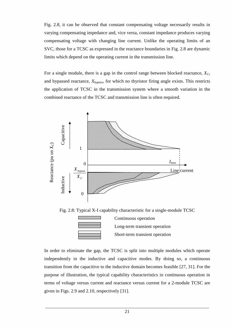
______________________________________________________________________
21
Fig. 2.8, it can be observed that constant compensating voltage necessarily results in
varying compensating impedance and, vice versa, constant impedance produces varying
compensating voltage with changing line current. Unlike the operating limits of an
SVC, those for a TCSC as expressed in the reactance boundaries in Fig. 2.8 are dynamic
limits which depend on the operating current in the transmission line.
For a single module, there is a gap in the control range between blocked reactance, XC,
and bypassed reactance, Xbypass, for which no thyristor firing angle exists. This restricts
the application of TCSC in the transmission system where a smooth variation in the
combined reactance of the TCSC and transmission line is often required.
Fig. 2.8: Typical X-I capability characteristic for a single-module TCSC
Continuous operation
Long-term transient operation
Short-term transient operation
In order to eliminate the gap, the TCSC is split into multiple modules which operate
independently in the inductive and capacitive modes. By doing so, a continuous
transition from the capacitive to the inductive domain becomes feasible [27, 31]. For the
purpose of illustration, the typical capability characteristics in continuous operation in
terms of voltage versus current and reactance versus current for a 2-module TCSC are
given in Figs. 2.9 and 2.10, respectively [31].
Line current
1
Imax 0
Cap
aciti
ve
Indu
ctiv
e
Rea
ctan
ce (
pu o
n XC)
C
bypass
X
X
0

______________________________________________________________________
22
Fig. 2.9: Typical V-I capability characteristics for a 2-module TCSC
Both TCSC modules operate in a capacitive region
One TCSC module operates in a capacitive region, the other in an inductive
region
Both TCSC modules operate in an inductive region
Fig. 2.10: Typical X-I capability characteristics for a 2-module TCSC
Both TCSC modules operate in a capacitive region
One TCSC module operates in a capacitive region, the other in an inductive
region
Both TCSC modules operate in an inductive region
Imax
Line current
0
Cap
aciti
ve
Indu
ctiv
e
Rea
ctan
ce (
pu o
n XC)
Line current 0
(Cap
aciti
ve)
(Ind
uctiv
e)
Vol
tage
(pu
on X
CI R
ate
d)

______________________________________________________________________
23
The larger the number of the modules into which the TCSC is divided, the narrower the
gap between the capacitive and inductive regions. With a sufficient number of modules,
the TCSC reactance can vary continuously from capacitive value to inductive value, and
the reactance limits approach a closed locus within which TCSC operation is feasible.
On this basis, the steady-state TCSC model will be presented and discussed in the
following.
In Fig. 2.11 is shown a circuit model where the TCSC is represented as a variable
reactance in series with the transmission line [32].
Fig. 2.11: TCSC steady-state model
The TCSC can be used to compensate a transmission line reactance to a certain level or
to control active-power flow to a specified value. In the former, the TCSC is expressed
by a series branch with the reactance value being given by the transmission line
compensation level. In the latter, the TCSC reactance is a control variable and the
control objective is represented by a control function as follows:
linespline PP = (2.12)
In (2.12):
Plinesp is the specified value, and
Pline is the active-power flow in the transmission line where the TCSC is used to
control its active-power flow to a specified value. Pline is a function of the voltages
at the sending and receiving ends of the transmission line as given in Appendix B.
The operating constraints of a TCSC are associated with its reactance and can be
expressed in terms of the following inequalities:
jXtcsc stcsc rtcsc
transmission line
Pline

______________________________________________________________________
24
maxcsccscmincsc ttt XXX ≤≤ (2.13)
In (2.13), Xtcscmin and Xtcscmax are the minimum (capacitive) and maximum (inductive)
limits of TCSC reactance. They are dynamic limits which depend on the transmission
line current and can be determined using the capability characteristics of the TCSC as
shown in Fig. 2.10. If the TCSC reactance hits a limit, the control function specified in
(2.12) is no longer applicable, and the TCSC behaves like a fixed reactance with the
value taking the respective limit value.
2.3.4 Static synchronous compensator (STATCOM)
The first STATCOM in the world using force-commutated thyristor inverter is rated at
20 MVAr which was developed and put into operation in January 1980 by Kansai
Electric Power Co., Inc. (KEPCO) and Mitsubishi Motors, Inc. [33]. In October 1986,
the first STATCOM employing high-power gate turn-off thyristor (GTO) inverters
developed by EPRI and Westinghouse Electric Company with the rating of ±1 MVAr
was put into operation [34]. Since then, STATCOMs have been developed and
implemented intensively in power systems for dynamic compensation which provides
voltage support, transient stability and damping improvements.
The basic principle of the STATCOM is to use voltage source converter (VSC)
technology based on power electronic devices (gate turn-off (GTO) thyristor or
insulated gate bi-polar transistor (IGBT)) that have the capability to interrupt current
flow in response to a gating command. This allows the STATCOM to generate an AC
voltage source at the converter terminal at the desired fundamental frequency with
controllable magnitude. A block diagram of a STATCOM is given in Fig. 2.12 [27].
The voltage difference across the coupling transformer reactance produces active- and
reactive-power exchanges between the network and the STATCOM. The exchange of
reactive-power with the network is obtained by controlling the magnitude of the voltage
source, whilst the exchange of active-power results from a control of the phase angle of
the voltage source. The active-power exchange is only used to control the DC voltage of

______________________________________________________________________
25
the capacitor. In steady-state condition where the capacitor voltage is constant, the
active-power exchange is, therefore, zero if the VSC losses are discounted.
Fig. 2.12: STATCOM schematic diagram
There are several VSC structures currently in use in actual power system operation.
Fig. 2.13 shows the basic structure of a three-phase, full-wave converter having six
switches with each consisting of a GTO thyristor connected in antiparallel with a diode.
Fig. 2.13: Basic VSC structure
With the aim of producing an output voltage waveform as near to a sinusoidal
waveform as possible, the switching of individual GTO thyristors in the VSC are
controlled by the switching control module designed to minimise the harmonics
Output
+
_
Va
Vb
Vc
. . . .
. .
coupling transformer
voltage source
converter
hsta
lsta
+ _
Plsta
Ista
Vdc

______________________________________________________________________
26
generated in the VSC operation and requirement for harmonic filters. There have been
three feasible solutions for the switching control strategies [35]: fundamental frequency
switching (multi-pulse converter), pulse-width modulation and multi-level converter:
(i) Fundamental frequency switching [33, 34, 36, 37]: The switching of each GTO
thyristor/IGBT is limited to one turn-on and one turn-off per supply-frequency cycle.
Implementing this switching strategy, the basic VSC structure in Fig. 2.13 yields a
quasi-square-wave output. With this switching scheme, there will be 6-pulses per cycle
in the VSC in Fig. 2.13. The key drawback of this switching strategy is that of
generating an unacceptable high harmonic content. In order to achieve better waveform
quality and higher power ratings, several six-pulse VSCs supplied from several
transformer secondary windings with appropriate phase shifts between them are
implemented to form a higher pulse structure. The key disadvantage is in the
complexity of the transformer arrangement required.
(ii) Pulse-width modulation (PWM) [37 – 39]: This control technique enables the
switches to be turned on and off at a rate considerably higher than the fundamental
frequency. The output voltage waveform comprises a series of rectangular pulses the
widths of which are modulated through the switching control. Undesirable harmonics in
the output waveform are shifted to the higher frequencies, therefore filtering
requirements are reduced considerably. Although many PWM control techniques have
been proposed, the sinusoidal PWM scheme is still the most popular because of its
simplicity and effectiveness.
(iii) Multi-level converter [40, 41]: In this configuration, the DC capacitor is split into
several units, each designed for the same fraction of the total DC bus voltage. Through a
switch construction consisting of power electronic switches (diode and GTO
thyristors/IGBTs), the AC output can be placed at any of these capacitor voltage levels,
thereby generating step waveforms closer to the sinusoidal waveform. This approach
requires a large number of switches and a complex control system but reduces the
complexity in the transformer arrangement. The multi-level configurations can be
applied to both fundamental frequency switching and pulse-width modulation strategies
to enhance their harmonic performance.

______________________________________________________________________
27
The steady-state control objective of the STATCOM is that of voltage control which is
expressed in terms of a V-I characteristic given in Fig. 2.14 [27]. The STATCOM
operating current limits in the characteristic of Fig. 2.14 derive from the current limits
of the semiconductor devices in the VSC.
Fig. 2.14: STATCOM V-I characteristic
Drawing on the V-I characteristic in Fig. 2.14 and referring to the schematic diagram of
STATCOM in Fig. 2.12, the steady-state model of the STATCOM will be derived in the
following.
Similar to the SVC, the first power-flow equation of the STATCOM model is that
which describes the voltage control function. Within the control range represented by
the minimum current, Istamin, and the maximum current, Istamax, the voltage magnitude at
the high-voltage side node is controlled according to the following linear function:
stastastarefhsta IaVV +=|| (2.14)
In (2.14):
|Vhsta| and Vstaref are the voltage magnitude at the high-voltage node and its
reference, respectively;
asta is the STATCOM reactance slope, and
Ista
|Vhsta|
0
Vrefsta
Under voltage protection
Istamax Istamin
capacitive inductive
Overvoltage protection

______________________________________________________________________
28
Ista is the STATCOM current which is an algebraic quantity determined in the same
way as the SVC current. Expression of Ista is given in Appendix B.
From the characteristic in Fig. 2.14, it can be seen that the operating constraints of a
STATCOM are those relating to the STATCOM current:
maxmin stastasta III ≤≤ (2.15)
In (2.15):
Istamax is the maximum current limit (maximum inductive current), and
Istamin is the minimum current limit (minus sign of maximum capacitive current).
If the STATCOM current hits a limit, the voltage control function specified in (2.14) is
no longer applicable and the STATCOM behaves like a current source with the current
taking the respective limit value.
The second equation describing the STATCOM steady-state condition is associated
with active-power injection at the low-voltage node of the STATCOM. It can be
assumed that the active-power loss in the STATCOM is small enough to be discounted.
This leads to the following equation [28]:
0=lstaP (2.16)
In (2.16), Plsta is the active-power injection into the coupling transformer from its low-
voltage node which is a function of nodal voltages as given in Appendix B.
2.4 FACTS DEVICE CONTROLLER
2.4.1 General
In general, FACTS devices have the functions of voltage magnitude, active- and
reactive-power flow controls. The required input signals to the FACTS device
controllers are those representing the supply-frequency components of power system
voltages and currents in the positive-phase sequence. From these components, voltage

______________________________________________________________________
29
magnitude, active- and reactive-power flows are formed, and then compared with the
input reference values for the control purpose as shown in Fig.2.15.
Fig. 2.15: FACTS controller block diagram
In Fig 2.15:
ia(t), ib(t), ic(t): measured current waveforms obtained from CTs in phases “a”, “b”
and “c” respectively;
va(t), vb(t), vc(t): measured voltage waveforms obtained from VTs or CVTs
respectively in phases “a”, “b” and “c”.
2.4.2 FACTS controller input signal derivation
A key step is to derive the supply-frequency components in the positive-phase sequence
of voltages and currents, following their measurements by voltage and current
transducers. The data acquisition system (DAS) converts the measured voltage and
current waveforms to discrete-time signals for subsequent processing and control signal
derivation. The discrete-Fourier transform (DFT) is applied to evaluate the supply
frequency components of voltages and currents in the phase variables which are
expressed in a phasor form. These phase-domain phasors are then transformed in a
straightforward manner to those in the positive-phase sequence, using the symmetrical
phase-sequence transformation. For example, if Va, Vb and Vc are the voltage phasors in
Data acquisition
system (DAS)
ia(t) ib(t) ic(t)
va(t)
vb(t)
vc(t)
Derivation of the supply-frequency components of
voltage and current in the positive-phase
sequence
Voltage magnitude and power
calculations
FACTS controller Σ
+
_
References

______________________________________________________________________
30
phases “a”, “b” and “c” respectively, then the positive-phase-sequence voltage phasor,
V1, is:
)..(31 2
1 cba VaVaVV ++= (2.17)
In (2.17):
oa 1201∠= (2.18)
The DFT has a good performance in extracting the supply-frequency components, even
when the waveforms have other frequency components such as harmonics. However,
there can be a concern in relation to the response time delay, particularly in the context
of high-speed FACTS controllers. With the DFT, a time delay of one supply-frequency
cycle (i.e. 20 ms in the 50 Hz power system) can be incurred. Therefore, there has been
a proposal for using the dq0 transformation method for extracting the supply-frequency
component from the phase-domain waveforms [42, 43]. The method is discussed in the
following section, with particular reference to the derivation of the voltage/current
phasor in the positive-phase sequence.
2.4.3 Application of the dq0 transformation for phasor calculation
Originally, the dq0 transformation was applied in 3-phase synchronous machine
modelling. The key advantage with the machine model formed in the dq0 frame of
reference is that the machine parameters are constant, which facilitates the analysis of
power systems where synchronous machines are a part. A beneficial by-product of the
transformation is that, in balanced operating condition free from harmonic distortion,
the three phase voltages or currents will transform at any time instant to constant d- and
q-axis components which can then be interpreted as a constant phasor at the supply
frequency in the positive-phase sequence. The following example will illustrate this
property of the dq0 transformation.
For a particular operation, the three phase voltages in phases “a”, “b” and “c” at a node
in a power system are given by, respectively:

______________________________________________________________________
31
)sin()( ϕω += tVtv ma (2.19)
)3
2sin()(
πϕω −+= tVtv mb (2.20)
)3
2sin()(
πϕω ++= tVtv mc (2.21)
The voltage waveforms in (2.19) – (2.21) are balanced and free from harmonic
distortions.
In general, the d-, q- and 0-components are related to the phase-domain components by,
using the dq0 transformation:
+−−−−
+−
=
)(
)(
)(
2
1
2
1
2
1
)3
2sin()
3
2sin()sin(
)3
2cos()
3
2cos()cos(
3
2
0 tv
tv
tv
ttt
ttt
v
v
v
c
b
a
q
d πωπωω
πωπωω
(2.22)
From the above relation, the d-, q- and 0-components of the voltages are, for any time
instant:
)sin(ϕmd Vv = (2.23)
)cos(ϕmq Vv −= (2.24)
00 =v (2.25)
It can be seen from (2.23) and (2.24) that vd and vq are constant while v0 is zero.
Moreover, the magnitude of the sinusoidal quantities can be calculated directly based on
the d- and q-components:
22qdm vvV += (2.26)
The supply-frequency voltage phasor in the positive-phase sequence is also formed
directly from the d-, q-components in (2.23) and (2.24).

______________________________________________________________________
32
The property allows the supply-frequency phasor in the positive-phase sequence to be
determined instantaneously from the phase-domain waveforms. This represents the key
advantage of the dq0 transformation over the DFT technique in relation to the supply-
frequency phasor calculation. However, this advantage is lost completely if there are
unbalances in the phase-domain waveforms or frequency components other than that at
the supply-frequency [44]. The following situations will impair the performance of the
dq0 transformation when applied for supply-frequency phasor calculation:
• Unbalanced operating condition in power system due to load unbalances and/or
transmission line parameter asymmetries
• Unbalanced or asymmetrical faults in power systems
• Harmonics in power systems due to nonlinear loads and/or controllers. For
example, FACTS controllers will introduce harmonics in their operation
• The presence of transients in power system due to disturbances. These transients
will have a wide range of frequencies in addition to the supply frequency.
The above situations will lead to:
• The d-, q-components being oscillatory functions of time
• The phasor formed from the d- and q-components not representing the positive-
phase sequence component of voltage or current. When this is the case, the
intended control function based on the positive-phase sequence components of
voltage and current will not be achieved
• The introduction of harmonics or frequencies other than the supply-frequency
into the input control signals to FACTS controllers. This will cause the
controllers to respond to harmonics, which is not an intended control function.
2.5 SYSTEM MODEL
The models of the SVC, TCSC and STATCOM expressed in terms of equations and
operating constraints in Section 2.3 augment directly the system power-flow equations
in (2.2) and constraints in (2.3) to give the complete power system model. The vector of
control variables, u, in (2.2) and (2.3) is extended to include those of the FACTS device
controllers.

______________________________________________________________________
33
2.6 CONCLUSION
Drawing on the well-established steady-state models for conventional items of plant
together with shunt and series FACTS devices, the nonlinear power-flow equation set
together with the operating constraints for the complete power system are assembled
which gives a foundation for the analysis and online control coordination to be
developed subsequently in details in the thesis.
The next chapter will focus on a more recent FACTS device where both shunt and
series controllers are combined in the one system, referred to as the unified power flow
controller (UPFC). The UPFC offers a high level of control flexibility and a wide range
of control functions together with their priorities. UPFC modeling is, therefore, a
challenging task which will be reviewed in the next chapter.

______________________________________________________________________
34
Chapter 3
Review of
Steady-State Models of UPFC
3.1 INTRODUCTION
In the previous chapter, the models of FACTS devices which are widely-used including
SVC, STATCOM and TCSC have been presented. These devices provide either shunt
or series compensation to a transmission system. With the recent advances in VSC
technology, it has been feasible to combine both shunt and series compensators in the
one system. The combined compensator, often referred to as the unified power flow
controller (UPFC), has been developed, and applied in transmission systems for
providing a number of compensation functions.
The unified power flow controller concept was first proposed by Gyugyi in 1991 [45].
The first UPFC was installed at Inez substation in eastern Kentucky, USA, to provide a
voltage support at Inez substation and optimise the utilisation of the new high capacity
line between Big Sandy and Inez stations [17]. Since its introduction, there have been
extensive research works reported in the literature on the modeling of the UPFC.

______________________________________________________________________
35
The UPFC is capable of controlling, simultaneously or selectively, all the three
parameters affecting power flow in the transmission line (voltage, impedance and phase
angle). In addition to voltage control function, the flexibility allows independent control
of active- and reactive-power flow in the transmission line for which the UPFC provides
the compensation.
While each of the SVC, STATCOM and TCSC discussed in the previous chapter can
provide only one control function in steady-state operation, the UPFC has multiple
control functions with different levels of priority to be observed when one or more
operating limits are reached in the operation. Therefore, a key challenge in developing a
UPFC model is that of representing individual control priorities among the control
functions in ensuring that the equilibrium condition predicted by the model reflects
closely or accurately the actual UPFC steady-state operation subject to multiple
operating limits.
The challenge has led to extensive research in UPFC modeling since the introduction of
the UPFC concept. There are numerous publications in the open literature on this topic
which is the subject of the review to be undertaken in this chapter. The review will also
identify and discuss key disadvantages of the models previously proposed. To facilitate
the review and discussion, the UPFC structure and its operating principle are first
described in the next section.
3.2 UPFC STRUCTURE AND OPERATING PRINCIPLES
The UPFC consists of two voltage source converters (VSC), as illustrated in Fig. 3.1,
namely, shunt converter and series converters [45]. These back-to-back converters share
a common capacitor on their DC side and a unified control system. The structure of
each of the 3-phase converters in Fig. 3.1 is shown in a schematic or block diagram
form only. The detailed structure in practice is more complex, and discussed in Section
2.3.4 of Chapter 2 in relation to the converter topologies together with the switching
schemes for reducing harmonic distortions arising from converter operation. This
arrangement functions as an AC-to-AC power converter in which the active-power can
flow in either direction between the AC terminals of the two converters, whilst reactive-

______________________________________________________________________
36
power can be independently generated (or absorbed) by each converter at its own AC
output terminal.
Fig. 3.1: UPFC representation as two back-to-back voltage source converters
The series converter provides the series compensation function of the UPFC by
injecting a voltage source VB with controllable magnitude |VB| and phase angle θB in
series with the transmission line via a series converter coupling transformer. The
voltage source (VB) can be controlled without restrictions if its magnitude is within a
specified maximum value, VBmax. The phase angle, θB, can be chosen between 0 and 2π
radians independently of the transmission line current.
Similar to a STATCOM, the shunt converter of a UPFC provides the voltage control
function as described in Chapter 2. In terms of the UPFC shunt converter operation, a
VB
+ _
. . . .
. . . .
. . . .
. . . . . . . . . .
. .
controller
+ _
Vdc
ac ac
shunt converter series converter
shunt converter coupling transformer
series converter coupling transformer
transmission line
measured
variables
parameter setting
references
. .
.
.
K L
switching signals
M
VE

______________________________________________________________________
37
shunt voltage source, VE, is generated at the converter terminal. The voltage control
function is achieved by controlling the magnitude of the shunt voltage source. However,
it is the DC link between the shunt and series converters that provides the control
flexibility which is not achieved with two separate compensators of the form discussed
in Chapter 2. The DC link in the UPFC structure of Fig. 3.1 provides the mechanism by
which the active-power is exchanged between the shunt and series converters. On this
basis, there are, in general, active-power components, in addition to reactive-power
ones, associated with the voltage sources generated from the converter operations. This
allows independent control of active- and reactive-power flows in the transmission line.
The parameters of the controller in Fig. 3.1 include the control system gains together
with time constants and UPFC voltage/current operating limits. These parameters are
pre-determined and set in the controller prior to its operation.
The switchings of individual GTO thyristors or IGBTs in the converters in Fig. 3.1 are
generated by the controller. The switching signals are determined to achieve the
minimum errors between the controlled variables obtained from measurements and their
references.
3.3 POWER LOSSES IN UPFC OPERATING CONDITION
Apart from those incurred in the converter coupling transformers, the losses in a UPFC
arise from the semiconductor switching devices together with the DC link.
The power loss in the DC link in the UPFC depends on the DC side current determined
by the required operating current levels on the AC side. Although the operating current
levels can be high, the power loss here is not a major one, given the short length of the
DC link in the UPFC. However, the power losses associated with the semiconductor
devices operation can represent a concern in relation to UPFC operational limits. These
UPFC power losses are mainly due to the forward biased voltage (i.e. the on-state
voltage) and the finite times required in turning on and turning off the practical
switching devices.

______________________________________________________________________
38
If I0 is the operating current level in the switching device, then the power losses are
classified into three types: on-state power loss, turn-off transition loss and turn-on
transition loss, as described in the following [46]:
s
ononstateonloss T
tIVP 0)( =− (3.1)
)(0)( 21
offcsdoffturnloss tfIVP =− (3.2)
)(0)( 21
oncsdonturnloss tfIVP =− (3.3)
In (3.1) – (3.3):
Ploss(on-state), Ploss(turn-off) and Ploss(turn-on) are average power losses during on-state,
turn-off transition, turn-on transition, respectively, of the semiconductor device;
Vd is the semiconductor device off-state voltage;
Von is the semiconductor device on-state voltage;
I0 is the semiconductor device on-state current;
fs is the switching frequency;
tc(on) is the turn-on transition time interval which is measured from the time instant
when the current starts rising (from zero) to the time instant when the voltage
achieve a small on-state value of V0;
tc(off) is the turn-off transition time interval which is measured from the time
instant when the voltage starts increasing (from the small on-state value) to the
time instant when the current reach to zero;
Ts is the switching time period.
The sum of the power losses in (3.2) and (3.3) is referred to as the switching power loss
which is directly proportional to the switching frequency. Equations (3.2) and (3.3)
indicate that the switching losses can be reduced by decreasing the switching frequency.
In UPFC operation, it is desirable to have a switch frequency as high as possible so that
the low-order harmonics will be minimal, and the waveform distortions are confined

______________________________________________________________________
39
mainly in the high frequency band. When this is the case, the harmonic filtering
requirements on the AC sides of the UPFC will be substantially reduced as the AC side
impedance themselves provide very effectively the filtering functions in the high
frequency band.
The finite turn-on and turn-off times of the switching device which lead to higher power
loss at high switching frequency ultimately impose an upper feasible limit on the
switching frequency. A principal aim in the UPFC design is to achieve a low overall
loss, taking into account the maximum UPFC operating currents. On this basis, it is
essential to represent the UPFC loss in the modelling at the UPFC design stage. The
loss is in general a nonlinear function of the UPFC operating current, given that there
will be some dependence on the current level of the switching device turn-on and turn-
off times.
However, if the main focus is on the study and control of a power system of which
UPFCs are a part, the UPFCs power losses will have only secondary effects on the
overall power system response which are often discounted without having any impact
on the engineering decision. Extensive reviews of the published literatures on UPFC
models as presented in the subsequent sections confirm this view on the UPFC power
losses.
3.4 UPFC CONTROL MODES AND OPERATING LIMITS
This section describes the steady-state control modes of which the UPFC is capable in
providing the compensation for the transmission line. Subject to the UPFC operating
limits, a wide range of power system quantities and parameters can be controlled to
specified values for achieving system operating requirements or benefits.
3.4.1 Shunt Converter
As discuss in Section 3.2, there are active- and reactive-power components associated
with the shunt voltage source arising from the shunt converter operation. The active-
power component is exchanged with that required by the series converter in

______________________________________________________________________
40
contributing to the active-power flow control in the transmission line. However, it is the
reactive-power component that is the principal one relevant to voltage or reactive-power
control at busbar K in Fig. 3.1. There are two control modes for the shunt converter:
reactive-power control mode and voltage control mode [18].
(i) Reactive-power control mode
In reactive-power control mode, the reference input is a signal representing the required
reactive-power injection at the busbar to which the shunt converter is connected and
identified by K in Fig. 3.1. In practice, it is preferable to control the shunt converter
current instead of directly controlling the reactive-power, as the shunt converter
operating limits are expressed in terms of current. Therefore, the reactive-power
reference is first transformed into equivalent reactive current component which is then
fed into the shunt current controller.
(ii) Voltage control mode
Similar to the reactive-power control mode, voltage control is based on the control of
the shunt converter reactive current component. However, the equivalent reactive
current required is determined by the outer voltage control loop with the objective of
achieving the required steady-state voltage/current characteristic defined by the
reference for the voltage at busbar K in Fig. 3.1 and slope reactance. The output of this
voltage control loop is interpreted as the required reactive current for use in the inner
shunt converter current control loop.
3.4.2 Series Converter
As discussed in Section 3.2 in relation to the UPFC operating principles, the series
converter together with its controller will generate a variable voltage in series with the
line in achieving a wide range of system operating requirements. The individual
requirements are, in general, expressed in terms of control modes to be specified and
implemented by the UPFC series converter controller [18].

______________________________________________________________________
41
(i) Direct voltage injection mode
The series converter generates a voltage phasor with magnitude and phase angle
specified by the reference inputs. A special case of this control mode is that of
compensation for the transmission line series reactance in which the injected voltage is
kept in quadrature with the line current. In this case, the level of the series compensation
depends on the value of the reference for series voltage magnitude.
(ii) Phase angle shifter emulation mode
The series converter injects an appropriate voltage so that the voltage at busbar L is
phase shifted relative to the voltage at busbar K in Fig. 3.1 by an angle specified by the
reference input. This control mode is used to control mainly the active-power flow in
the transmission line.
(iii) Line impedance emulation mode
The series voltage injected is controlled to the value proportional to the line current so
that the series converter transformer together with the series converter is equivalent to
an impedance the value of which is specified by the reference input. In order to avoid
resonance or instability caused by a negative resistance or capacitive reactance, the
reference value of the impedance has to be chosen carefully. In this mode of control, the
total resistance and reactance of the interconnection between busbars K and M in Fig.
3.1 can both be reduced, which provides a more effective series compensation in the
case of lines with high resistance.
(iv) Power flow control mode
In this mode, the series converter can control both the active- and reactive-power flows
independently in a transmission line by regulating the series injected voltage in both
magnitude and phase angle. The injected voltage is determined automatically and
continuously to maintain the desired active- and reactive-power despite system changes.
Among many FACTS devices available at present, only the UPFC has this versatile

______________________________________________________________________
42
mode of control, which provides the optimal operation of the line in terms of both
active- and reactive-power flows.
3.4.3 Stand alone shunt and series compensation
The UPFC circuit structure offers the possibility of operation in which the two
converters can operate independently of each other by disconnecting the DC link and
splitting the DC capacitor bank [18]. In this case, the shunt converter operates as a
STATCOM and the series converter as a static synchronous series compensator (SSSC).
This kind of operation is applied to handle the contingencies in which failure of either
of the converters occurs, or adapt to the future change of system requirement in which
either shunt or series compensation is required of both converters. Because of the
disconnection of the DC link in this operation mode, neither converter is capable of
exchanging the active-power with the system. This limits the flexibility of the separate
shunt and series compensators in power system control. In the stand alone operation, the
series converter controller needs to be modified to provide the DC voltage control.
3.4.4 Operating limits
The operating modes presented above are subject to the operating limits of the shunt
and series converters including their transformers, the DC link together with the
transmission line voltage limits. The limits consist of the following ones [18, 27, 47]:
- Limit on the series injected voltage magnitude: The magnitude of the series injected
voltage is limited by the maximum voltage rating of the series converter. The series
converter and its associated transformer are designed to a specified maximum voltage
level. Operation beyond this level is not allowed.
- Limit on the series converter current: Depending on the rating of the series converter
and the coupling transformer, the series converter current has an allowable maximum
value.

______________________________________________________________________
43
- Limit on the shunt converter current: The shunt converter current has two components:
active and reactive. The active current component is controlled by the shunt converter
controller to achieve a constant DC link voltage in steady-state operation which, at the
same time, leads to the net interchange of active-power between the two converters is
zero if the UPFC losses are discounted. The reactive component, on the other hand,
relates to reactive-power supplied to or absorbed from the transmission system that
supports the voltage of the busbar on the high-voltage side of the shunt converter
transformer. In relation to the operating limit on the shunt converter current, the active
component is assigned to have, in general UPFC application, a higher priority than the
reactive one so that the DC link voltage control together with the active-power
requirement takes the precedence over reactive-power/voltage control at busbar K in
Fig. 3.1 when the shunt converter current reaches its limit.
- Limit on the active-power exchanged between the series and the shunt converters:
Because of the size and rating of the DC link and DC capacitor, the active-power
exchanged between the two converters has the upper limit.
- Lower and upper limits on the line-side voltage of the UPFC: The UPFC has the
intrinsic ability to raise or lower the voltage magnitude at busbar L in Fig. 3.1 by a large
fraction. Therefore, it will be necessary, in general, to impose lower and upper
allowable magnitude of the voltage at busbar L to satisfy the line voltage operating
limits.
Following the discussion of the UPFC control modes and operating limits, the
subsequent sections will review steady-state UPFC models which have been developed
and reported in the open literature.
3.5 DECOUPLED UPFC MODEL
Decoupled model of the UPFC was proposed in [48] where the UPFC operation is
decoupled into two separate ones at nodes K and L in Fig. 3.1 respectively. The model
development is based on the assumption of a control mode that the shunt converter
regulates the voltage magnitude at node K in Fig. 3.1 at a reference value, and the series

______________________________________________________________________
44
converter controls active- and reactive-power flows from node L to node K in Fig. 3.1
to pre-specified values. The block diagram of a power system with a UPFC together
with the controlled quantities are shown in Fig. 3.2:
Fig. 3.2: UPFC connection in power system
On the basis of the decoupling which separates nodes K and L as shown in Fig. 3.3, the
transmission line power flow is now equivalent to the nodal power at node L, with
specified values for active-power (Pref) and reactive-power (Qref). In this equivalent, the
UPFC operation at node L is represented, in steady-state power-flow analysis, as a load
node, or PQ node.
The separate operation at node K is described in terms of its specified voltage
magnitude (Vref) and nodal active-power. With the assumption that the losses in the
UPFC are negligible, the nodal active-power at node K will have the same magnitude as
that at node L but with an opposite direction as shown in Fig. 3.3. Therefore, the
operation at node K is equivalent to that of a generator node or PV node, for power-flow
model and analysis purpose.
Fig. 3.3: Decoupled UPFC model
power system
UPFC
K L
Vref
Pref
Qref
Pref
power system
K L
Pref + jQref
Vref
Pref

______________________________________________________________________
45
With the decoupled UPFC model in Fig. 3.3, a standard power-flow software system
can be applied to determine the power system steady-state solution, which also gives the
UPFC terminal voltages at nodes K and L together with the nodal reactive-power at
node K. From these known quantities, the UPFC voltage sources established by the
shunt and series converters as discussed in Section 3.2 are calculated [48].
Although the decoupled UPFC model is implemented directly, using any standard
power-flow software, it has inherently the key drawbacks as follows:
- The model is inflexible. It can only be applied if a UPFC is used to control voltage
magnitude, active- and reactive-power, simultaneously. The model is no longer
applicable when other control modes are required of the power system operation.
- It does not appear that the model takes into account UPFCs operating limits. Because
the UPFC operating condition is determined after the power flow solution procedure has
converged, it is impossible to resolve operating limits if they arise during the solution
process.
3.6 TWO-VOLTAGE SOURCE MODEL
On the basis of the UPFC operation in steady-state mode discussed in Section 3.2, the
two-voltage source model was derived and presented in [49] in which both shunt and
series voltage sources are used as variables in power-flow equations. The steady-state
UPFC model is expressed in terms of an equivalent circuit shown in Fig. 3.4 [49]. In the
circuit, each of the shunt and the series converters together with their coupling
transformers is represented by a variable voltage source in series with the leakage
impedance of the corresponding coupling transformer. Between the two voltage sources,
there is the active-power exchange.

______________________________________________________________________
46
Fig. 3. 4: UPFC equivalent circuit
In Fig. 3.4:
VE and VB are the variable voltage sources representing the shunt and series
converters, respectively;
IE and IB are the currents at the AC terminals of the shunt and series converters,
respectively, and
ZE and ZB are the leakage impedances of the shunt and series converter coupling
transformers.
Based on the circuit in Fig. 3.4, the residual functions associated with active- and
reactive-power at node K, fPK and fQK respectively, which take into account the
connection of the UPFC with the network, are given as follows:
KspiKiEEKBLBKKPK PVYYVVYVVVVf −+−+−+= ∑ }])()[(Re{ * (3.4)
KspiKiEEKBLBKKQK QVYYVVYVVVVf −+−+−+= ∑ }])()[(Im{ * (3.5)
Similarly, the residual functions associated with the active- and reactive-power at node
L, fPL and fQL respectively, where there is not any load demand, are:
}]).[(Re{ *∑+−−= iLiBBKLLPL VYYVVVVf (3.6)
}]).[(Im{ *∑+−−= iLiBBKLLQL VYYVVVVf (3.7)
VE
VB
ZE
ZB
IB
IE
transmission line
active-power exchange
K L

______________________________________________________________________
47
In (3.4) – (3.7):
VK and VL are voltage phasors at nodes K, L in Fig. 3.4, respectively;
Vi is the voltage phasor at node i of the system which is connected directly to node
K or node L of the UPFC;
YE = 1/ZE, where ZE is the leakage impedance of the shunt converter coupling
transformer;
YB = 1/ZB, where ZE is the leakage impedance of the shunt converter coupling
transformer;
YKi is the element (K,i) of the network nodal admittance matrix;
PKsp and QKsp are the specified active- and reactive-power load demand at node K;
Re{.} and Im{.} denote the real part and imaginary part of a complex expression,
respectively, and
Superscript * denotes complex conjugate.
On assuming a lossless converter operation, the active-power supplied or absorbed by
the shunt converter must be equal to the active-power absorbed or supplied,
respectively, by the series converter. In other words, the total active-power of the shunt
and series converters is zero, which leads to the following residual function:
}))((Re{}))((Re{ **BBKLBEKEEPEB YVVVVYVVVf −−+−= (3.8)
In (3.8), fPEB is the residual function associated with the net active-power exchange
between the UPFC and the network.
Five residual functions in (3.4) – (3.8) form one part of the steady-state model of the
UPFC based on the UPFC topology and the coupled relation between the shunt and
series converters in terms of active-power exchange. Because there are eight unknowns
which are magnitudes and phase angles of voltages of the shunt and series voltage
sources and those at nodes K and L in Fig. 3.4, there is a need to develop three more
residual functions to form the complete model of the UPFC. Other three residual
functions will be derived based on the control modes of the shunt and series converters
in which the control functions for each converter are specified. For instance, if the

______________________________________________________________________
48
UPFC operates in the control mode in which the shunt converter controls the voltage
magnitude at node K, and the series converter controls the active- and reactive-power in
the transmission line connecting to node L in Fig. 3.4, the three residual functions are as
follows:
refKVupfc VVf −= || (3.9)
refBBKLLPupfc PYVVVVf −−−= })).((Re{ * (3.10)
refBBKLLLupfc QYVVVVf −−−= })).((Im{ * (3.11)
In (3.9) – (3.11):
fVupfc, fPupfc and fQupfc are the residual functions associated with the voltage, active-
and reactive-power controls, respectively, of the UPFC;
Vref is the reference value for the voltage magnitude at node K, and
Pref and Qref are the reference values for the active- and reactive-power flows in the
transmission line.
The two-voltage source model reviewed above is suitable for incorporation into existing
Newton-Raphson (NR) power-flow algorithm. The main feature of the model is the use
of the series voltage sources as variables. This leads to two key disadvantages:
(i) There is a possibility of divergence in the NR solution sequence if the initial
values for the series voltages are not close to the final solution [50]. It is acknowledged
that, in the normal power-flow problem, a flat starting voltage profile (e.g. o01∠ pu) for
nodal voltages is a suitable initial condition to achieve a quadratic convergence in NR
solution sequence. However, if the shunt and series voltage sources of the UPFC are
included in the variables of the power system study problem, the issue of estimating the
starting condition for these variables becomes more involved. To cope with this
problem, in [49], the initial condition estimations for the magnitudes and phase angles
of the series and shunt voltage sources have been proposed:

______________________________________________________________________
49
21
20
0 )( CPV
XV ref
L
BB += (3.12)
)||
(tan1
10
C
PrefB
−=θ (3.13)
10 =EV (3.14)
−= −
BKE
BEBLKE XVV
XVVV00
000010 )sin()(
sinθθ (3.15)
where )( 000
1 KLB
Lref VV
X
VQC −−= (3.16)
In (3.12) – (3.16):
0BV and 0
Bθ are the initial values for magnitude and phase angle of the series
voltage;
0EV and 0
Eθ are the initial values for magnitude and phase angle of the shunt
voltage;
0KV and 0
LV are the initial values for voltage magnitudes at node K and node L in
Fig. 3.6, respectively, and
XB and XE are the inductive reactance of the series and shunt coupling
transformers which are assumed to be lossless.
The procedure for estimating the UPFC series and shunt voltage above uses the
specified active- and reactive-power references on the basis that the UPFC is used to
control both transmission line active- and reactive-power flows. However, it is not
always the case in general. Even if both active- and reactive-power flows are controlled,
the final solution for them might not be equal to the specified values, due to the UPFCs
operating limits, control priorities and system operating condition. In this case, the
estimation based on the specified references may not be a good one [50].
(ii) In some cases, the Jacobian matrix becomes singular or ill conditioned [50]. The
column of the Jacobian matrix formed from the partial derivatives of all of the residual
functions with respect to the phase angle of the series voltage have the following
nonzero elements, based on the residual functions in (3.4) – (3.8) and (3.10) – (3.11):

______________________________________________________________________
50
)sin(.||.||.|| BBKBBKB
PK YVVf αθθθ
−−=∂∂
(3.17)
)cos(.||.||.|| BBKBBKB
QK YVVf
αθθθ
−−−=∂∂
(3.18)
)sin(.||.||.|| BBLBBLB
PL YVVf αθθθ
−−−=∂∂
(3.19)
)cos(.||.||.|| BBLBBLB
QL YVVf
αθθθ
−−=∂∂
(3.20)
)sin(.||.||.||)cos(.||.||.|| BKBBKBBLBBLBB
PEB YVVYVVf αθθαθθθ
−−+−−−=∂∂
(3.21)
)cos(.||.||.|| BBLBBLB
Pupfc YVVf
αθθθ
−−−=∂
∂ (3.22)
)sin(.||.||.|| BBLBBLB
Qupfc YVVf
αθθθ
−−=∂
∂ (3.23)
In (3.17) – (3.23):
|VB| and θB are the magnitude and phase angle of the series voltage;
|VK| and θK are the magnitude and phase angle of the nodal voltage at node K;
|VL| and θL are the magnitude and phase angle of the nodal voltage at node L, and
|YB| and αB are the module and angle of the admittance of the series converter
coupling transformer.
Equations (3.17) – (3.23) show that all the nonzero partial derivatives with respect to
the series voltage phase angle contain the factor of |VB|. This factor in the UPFC
operation can be very small or close to zero in the final solution or during the iterative
solution sequence. As a consequence, the above Jacobian matrix elements can also be
very small or close to zero. In this case where each element of the column is zero or
close to zero, the Jacobian matrix becomes singular or ill-conditioned.

______________________________________________________________________
51
3.7 POWER INJECTION MODEL
Starting from the power injection model (PIM) developed in [51] for modeling phase-
shifting transformer which retains the symmetry in the network nodal admittance
matrix, it has been proposed that the same technique is to be extended to model other
FACTS devices although the advantage of PIM in relation to the symmetry in the
admittance matrix does not exist in many cases. The PIMs for the case of the UPFC
have been developed and reported in [52 – 54].
The PIM reported in [52] is derived by first transforming the series converter voltage
source in Fig. 3.5a into an equivalent current source between nodes K and L as shown
in Fig. 3.5b, based on the Norton’s equivalent. The current source is then interpreted as
the nodal currents at nodes K and L, with opposite directions. The PIM in Fig. 3.5c for
the series converter is formed by converting the nodal currents to nodal powers, using
voltages at nodes K and L.
Fig. 3.5: Current source and power injection model of the series converter
For the shunt converter, the voltage source together with the respective coupling
transformer impedance in Fig. 3.6a is first replaced by the equivalent current source in
parallel with the admittance, using the Norton’s equivalent, as given in Fig. 3.6 b. The
equivalent current source and its parallel admittance are then converted to the nodal
power using the voltage at node K as shown in Fig. 3.6c.
(b) (c)
(a)
VB ZB K L
B
B
Z
V
ZB K L
ZB
*
B
BL Z
VV
*
−
B
BK Z
VV
K L

______________________________________________________________________
52
Fig. 3.6: Current source and power injection model of the shunt converter
Combining the power injection model of the series converter in Fig. 3.5c and that of the
shunt converter in Fig. 3.6c yields the power injection model of the UPFC as a whole,
which is shown in Fig. 3.7.
Fig. 3.7: Power injection model of UPFC in [52]
In Fig. 3.7, PKinj and QKinj are the total active- and reactive-power injections of the
UPFC at node K, respectively.
})(Re{})(Re{ **
E
KEK
B
BKKinj Z
VVV
Z
VVP
−+−= (3.24)
})(Im{})(Im{ **
E
KEK
B
BKKinj Z
VVV
Z
VVQ
−+−= (3.25)
PLinj and QLinj in Fig. 3.7 are active- and reactive-power injections of the UPFC at node
L, which are determined as:
K
*
−
E
KEK Z
VVV
(c) (a)
VE
ZE
K K
EZ
1
E
E
Z
V
(b)
K
PLinj+jQLinj PKinj+jQKinj
L

______________________________________________________________________
53
})(Re{ *
B
BLLinj Z
VVP = (3.26)
})(Im{ *
B
BLLinj Z
VVQ = (3.27)
Based on the model in Fig. 3.7, it can be stated that, by using PIM, the UPFC
connecting between nodes K and L in Fig. 3.1 is modeled as the two power injections at
nodes K and L between which is the leakage impedance of the series converter coupling
transformer.
To incorporate the PIM of the UPFC in a power-flow program in which variables
consist of the magnitudes and phase angles of the nodal voltages, the nodal admittance
matrix is first modified by taking into account the presence of the impedance ZB
between nodes K and L. The residual functions associated with nodes K and L are then
modified by addition of appropriate injection powers:
KinjKspiKiKPK PPVYVf +−= ∑ )*}(Re{ (3.28)
KinjKspiKiKQK QQVYVf +−= ∑ )*}(Im{ (3.29)
LinjLspiLiLPL PPVYVf +−= ∑ )*}(Re{ (3.30)
LinjLspiLiLQL QQVYVf +−= ∑ )*}(Im{ (3.31)
Active- and reactive-power injections at node K and node L in (3.28) – (3.31), PKinj,
QKinj, PLinj and QLinj, are treated as dependent active- and reactive-power load demands,
which are calculated in every iteration using (3.24) – (3.27) in which the nodal voltages
VK and VL take the values determined in the previous iteration, and the magnitudes
together with phase angles of VE and VB are found by solving the four following
equations which are based on the control mode of the UPFC and the fact that the total
active-power of the series and shunt converters is zero. If the control mode is that of
voltage together with transmission line power flow control, then:
0|| =− refK VV (3.32)
0})).((Re{ * =−−− refBBKLL PYVVVV (3.33)

______________________________________________________________________
54
0})).((Im{ * =−−− refBBKLL QYVVVV (3.34)
0}))((Re{}))((Re{ ** =−−+−= BBKLBEKEEEB YVVVVYVVVP (3.35)
Different from the PIM of the UPFC reported in [52], in [53 – 55], the impedance of the
transmission line between nodes L and M connecting to the UPFC in Fig. 3.1 is
represented. This leads to the following PIM of the UPFC [53]:
Fig. 3.8: Power injection model of UPFC in [53]
In Fig. 3.8:
PKM0 and QKM0 are the components active- and reactive-power flows, respectively,
in the transmission line after the removal of the series voltage source, which are
functions of the voltage magnitudes and phase angles of nodes K and M;
PKinj and QKinj are the active- and reactive-power injections, respectively, of the
UPFC at node K;
PMinj and QMinj are the active- and reactive-power injections, respectively, of the
UPFC at node M, and
ZKM is the impedance of the transmission line.
To represent the transmission line reactive-power flow control in the formulation, the
reactive-power injection at node K, QKinj, in Fig. 3.8 is split equivalently into two
reactive-power components:
KKinjKMinjKinj QQQ += (3.36)
The component identified by QKMinj in (3.36) is that which combines with QKM0 to give
the total transmission line reactive-power flow at node K. The second component,
ZKM
PMinj+jQMinj PKinj+jQKinj
PKM0+jQKM0 K M

______________________________________________________________________
55
QKKinj, is the reactive-power injection from the shunt-converter operation related to the
voltage control function at node K.
The above decomposition leads to the decomposed PIM of the UPFC [53]:
Fig. 3.9: Decomposed power injection model of UPFC in [53]
When the UPFC operation is supposed to be lossless, the active-power injections at
nodes K and M have the same value but opposite directions:
0=+ MinjKinj PP (3.37)
Taking into account the presence of the UPFC power injections, the residual functions
associated with active- and reactive-power at nodes K and M are given as:
KinjKspiKiKPK PPVYVf +−= ∑ )*}(Re{ (3.38)
KMinjKKinjKspiKiKQK QQQVYVf ++−= ∑ )*}(Im{ (3.39)
KinjMspiMiMPM PPVYVf −−= ∑ )*}(Re{ (3.40)
MinjMspiMiMQM QQVYVf +−= ∑ )*}(Im{ (3.41)
In (3.38) – (3.41), the variables associated with the UPFC which take part in voltage
together with active- and reactive-power flows control of the UPFC are assembled to
form the control vector: [PKinj QKKinj QKMinj]T. The reactive-power injected at node M,
QMinj, is a variable. However, it can be expressed in terms of the control variables,
QKKinj and QKMinj. Therefore, for each UPFC, there are three additional independent
variables which form the control vector to be determined simultaneously with other
network variables.
ZKM
PMinj+jQMinj
jQKKinj
PKM0+jQKM0
PKinj+jQKMinj
M K

______________________________________________________________________
56
The decomposed PIM of the UPFC developed above combined with the optimisation
procedure for representing the UPFC control mode leads to the power flow control
approach which consists of two major modules: one for solving the optimisation
problem and the other for power flow calculation [55].
In the optimisation problem, the UPFC control mode is expressed in terms of the
objective function which is to be minimised with respect to control variables:
|)(||||||| 00 refKKinjKrefKMinjKMrefKinjKM VQVQQQPPPf −+−−+−−= (3.42)
The objective function in (3.42) is subject to equality constraints in terms of power-flow
equations some of which are the residual functions given in (3.38) – (3.41). The power-
flow equations in a linearised form provide the relationship expressed numerically
between |VK| and injected reactive-power, QKKinj, which is required in the optimisation.
The inequality constraints to which the objective function (3.42) is subject include the
operating limits of the UPFC in terms of the thermal limits of the shunt and series
converters transformers, and the active-power exchange between the two converters.
Constrained optimisation based on linear programming methodology has been
suggested in [55] for minimising the objective function in (3.42).
In the power flow calculation, the control vector [PKinj QKKinj QKMinj]T obtained by
solving the optimisation problem is used as specified powers for forming the power-
flow equations in (3.38) – (3.41).
Newton-Raphson method with optimal multiplier has been adopted in [55] to solve the
power-flow problem where each UPFC is represented by a set of nodal power injections
the values of which are tentatively determined from the solution of the optimisation.
Iterations in the optimisation-power flow loop are required until convergence is
achieved.

______________________________________________________________________
57
As many of the UPFC operating limits are, in practice, expressed in terms of voltages
and currents, the PIMs which are based on the transformation into nodal powers have a
difficulty in representing all of the practical limits encountered in UPFC operation.
Based on PIM for representing the UPFC, power-flow solution method has also been
developed where constrained optimisation is not required [54]. During the power-flow
solution sequence, UPFCs operating limits are not represented. Tentative solutions are
then used for checking against UPFC operating constraints. Depending on the outcome
of the checking, UPFCs parameters which include series and shunt voltage magnitudes,
shunt and series converter currents and active-power exchange between the two
converters are adjusted for complying with the specified limits.
Following the adjustments, a revised power-flow problem is formulated where the
UPFC injected powers are modified, and a new power-flow solution is obtained. Further
checking against UPFC operating limits will then be carried out, and the iterative
process of the power-flow-limits checking loop continues until all of the UPFC
parameters are within their specified limits.
In [54], a set of rules or strategies were presented, where associations between
individual UPFC operating limits and control variables/quantities based on extensive
studies are used, to resolve the constraint violation. The strategies adopted in [54] are
given in the following:
(i) If |VB| violates the constraint, fix it at its maximum value in the remaining
computation process,
(ii) In IB or PE is out of the limit range, set it at the limit value and then solve the θB
and/or |VB| using the associated equations,
(iii) If both IB and PE limits are violated, solve the |VB| and/or θB respectively at first,
then select the one which gives both IB and PE within the limits,

______________________________________________________________________
58
(iv) If IE is beyond the limit while |VE| is within the range, relax |VK| to alleviate IE and
use |VK| to obtain the associated reactive-power injection as to achieve the new
specified |VK|,
(v) If |VE| exceeds the limit, set it at the limit value and then use it to examine whether
IE is within its limit or not. If it leads to violation of IE repeat step (iv),
(vi) If both IE and |VE| are out of the range, use their limit values to solve the new
specified |VK|.
However, the basis for forming the above rules or strategies is an empirical rather than a
formal or mathematical one. Therefore, it cannot be said that the strategies proposed
have a general validity, particularly in the case of multiple UPFCs operations.
Both the UPFC PIM combined with constrained optimisation [55] and that with the
strategies for constraint resolution [54] have the disadvantages that:
(i) The shunt converter current limit in a dynamic form in which the active component
of this current has a higher priority than the reactive component is not represented.
(ii) Relative UPFC control priorities are not taken into account when one or more
operating limits are violated.
3.8 IDEAL TRANSFORMER UPFC MODEL
More recently, a new model for the UPFC based on ideal transformer with a complex
turns ratio and variable shunt admittance has been proposed in [56]. The model is an
approximate one the principal use of which is for identifying possible optimal locations
for installing UPFCs [57]. The UPFC operating limits together with control function
relative priorities which are not of a concern in the studies are not represented in the
model. The model is not suitable if accurate or detailed solutions for power-flow control
purpose are required.

______________________________________________________________________
59
3.9 CONCLUSIONS
The state-of-the-art models for the UPFC in steady-state condition have been reviewed.
These models have been incorporated into an existing FACTS Newton-Raphson power
flow analysis and implemented widely in research work in relation to power-system
analysis and control. Constrained optimisation methods have also been used in
combination with power-flow analysis algorithms.
However, in the models, there have been no developments for representing a systematic
procedure for constraint resolution, given that there are nonlinear interactions among the
constraints, and at the same time representing the specified priority in control when one
or more UPFC operating limits are violated in the solution sequence.
The shortcomings of the existing UPFC models lead to the motivation to develop a new
steady-state model based on the interpretation of the network variables during the
iterative power-flow solution process as dynamic ones, which allows the UPFC
controller together with its responses to be simulated, for any specified input references.

______________________________________________________________________
60
Chapter 4
Dynamic Simulation-Based UPFC
Steady-State Model
4.1 INTRODUCTION
The review in Chapter 3 has identified the difficulties encountered in the existing UPFC
steady-state models in relation to constraint resolution and relative control priority
representation. An approach based on representing the operation of the UPFC shunt and
series controllers directly during the iterative steady-state solution process will in a
straightforward manner resolve any operating limit violations subject to specified
control priorities.
The present chapter adopts the above approach for developing a new steady-state UPFC
model in which the UPFC controller dynamics are simulated during the power-flow
solution process. This is feasible as the power network variables which are updated at
each iteration can be interpreted as dynamic ones. If the Newton-Raphson (NR) method
is adopted for solving the power-flow problem, then the NR iterative step will take the
role of the time variable in dynamical systems. In this way, the dynamic responses of
the UPFC controllers can be simulated as the network variables change as the NR

______________________________________________________________________
61
iteration counter increases towards its final value at convergence.
Dynamic simulation of the UPFCs controllers will remove the assumption that the
specified UPFC control objectives have been achieved in previous UPFC models.
The new UPFC model for power-flow analysis is based on the explicit dynamic
simulation of both the shunt converter and series converter controllers. The dynamic
simulation is carried out in conjunction with the NR power-flow solution sequence. The
updated voltages at each NR iterative step are interpreted as dynamic variables. The
relevant variables are input to the UPFC controllers. The responses of controllers to the
inputs, subject to the limits and priority specified in the controllers, are the voltage
sources associated with the shunt and series converters. The voltage sources are input to
power network at the UPFC locations for the subsequent NR iteration. The constraint
resolution problem encountered in previous UPFC steady-state model in which there are
interactions among the UPFC equations representing the control objectives and
inequality constraints representing the operating limits is avoided completely. The
relative priority in UPFC control is inherently taken into account in the new formulation
via the direct simulation in a dynamical form of the UPFC controllers. The overall
simulation can be considered to be a hybrid one in which dynamic simulation-based
model of UPFC is combined with the NR power-flow model for power network.
The applications of the simulation technique are those in power systems planning and
design where UPFCs are proposed. With the general simulation technique developed in
the chapter, the use of TNA [18] for system study will be avoided.
The hybrid model together with its software implementation is validated using results
obtained from the power-flow study of a representative test system.
4.2 UPFC DYNAMICAL MODEL
To facilitate the discussion and development, the UPFC structure in Fig. 3.1 is shown in
a schematic form in Fig. 4.1. Based on a specific UPFC control mode where the shunt
converter regulates the voltage at node K, and the series converter controls the active-
and reactive-power flows in the transmission line connecting to node L in Fig. 4.1, the

______________________________________________________________________
62
UPFC model suitable for dynamic simulation in the power-flow solution procedure is
developed. However, the model development steps are general in principle, which can
be applied to any other control modes discussed in Chapter 3.
Fig. 4.1: The UPFC schematic diagram.
The UPFC model is formed in terms of two VSC controllers. Expressed in the time-
domain, the dynamical representation in a block diagram form of the shunt converter
controller is shown in Fig. 4.2 [18].
Fig. 4.2: Block diagram of shunt converter controller.
θE(t)
Voltage
Magnitude
Σ
Shunt Reactive Current Limiter
Σ
Σ
Σ
Active/Reactive Current
Components Calculator
Limit Calculator
IE(t)
VK(t)
Vref
Vdcref
Vdc(t)
IEq(t)
IEp(t)
IEqref(t)
IEpref(t)
VEq(t)
Magnitude and Angle Calculator
VEp(t) |VE(t)|
Σ
θK(t)
_
+
+
+
+ _
_
+
+ Phase
Locked Loop
VK(t)
_ Error Amplifier
and Controller
Error Amplifier
and Controller
Error Amplifier
and Controller
DC link
K
series converter
shunt converter
.
.
.
.
L transmission line

______________________________________________________________________
63
In Fig. 4.2:
VK(t) and Vref are the voltage phasor at node K at t and its magnitude reference,
respectively;
IE(t) is the shunt converter current phasor at t;
Vdc(t) and Vdcref are the DC voltage at t and its reference, respectively;
IEp(t) and IEq(t) are the in-phase and quadrature components, respectively, of the
shunt converter current at t with respect to the reference given by VK(t);
IEpref(t) and IEqref(t) are the in-phase and quadrature components, respectively, of
required shunt converter current at t;
VEp(t) and VEq(t) are the in-phase and quadrature components, respectively, of the
shunt converter voltage source at t;
|VE(t)| and θE(t) are the magnitude and angle, respectively, of the shunt converter
voltage source at t, and
θK(t) is the phase angle of voltage phasor VK(t).
The output from the shunt converter can be interpreted as a voltage source applied to the
power system at node K, the magnitude and phase angle of which are adjusted by the
controller to control the voltage magnitude at node K to a specified value, Vref, and keep
the DC voltage constant. In Fig. 4.2, t is the independent time variable. In the digital
implementation of the controller, the time variable takes a discrete form.
Similarly, the series converter controller in a block diagram form is given in Fig. 4.3.
The functions of the controller are to control active- and reactive-power flows in the
transmission line connecting to node L in Fig. 4.1. To achieve this control objective, the
series controller adjusts both the magnitude and phase of the series voltage which is
inserted into the transmission line.

______________________________________________________________________
64
Fig. 4.3: Block diagram of series converter controller
In Fig. 4.3:
VL(t) is the voltage phasor of node L at t;
IB(t) is the series converter current phasor at t;
Pref , Qref are the active- and reactive-power references, respectively;
VBp(t) and VBq(t) are the in-phase and quadrature component, respectively, of the
series voltage at t, and
|VB(t)| and θB(t) are the magnitude and phase angle, respectively, of the series
converter voltage at t.
The output signals from the controllers in Figs. 4.2 and 4.3 are input to the PWM
(pulse-width-modulation) control system of the converters to achieve the required 3-
phase voltage sources.
As described in Chapter 3, the operation of both the shunt and series converters are
Error Amplifier
and Controller
θB(t)
Series Injected Voltage Limiter
VBq(t)
Magnitude and Angle Calculator
VBp(t) |VB(t)|
Σ
θK(t)
Limit Calculator
VL(t)
VK(t)
IB(t)
Vdc(t)
VK(t)
Σ
Pref
IBp(t)
Qref
Active/Reactive Current
Components Calculator
IBpref(t)
Σ
IBq(t)
Active/Reactive Current
Components Calculator
IBqref(t)
IB(t)
+ _
+
_
+
+
Phase Locked Loop
VK(t)

______________________________________________________________________
65
subject to limits which include:
- Maximum series voltage magnitude
- Maximum series converter current
- Maximum shunt converter current
- Maximum line-side voltage of the UPFC
- Minimum line-side voltage of the UPFC
- Maximum active-power exchange between the series and shunt converters
These limits are represented in the controllers in forming the outputs in real time.
Separately, the UPFC has a second level of control by which the reference inputs to the
controllers are modified [18], when required, to achieve a pre-specified relative priority
in control functions. In general, modifications of reference inputs are needed when one
or more operating limits are violated.
For power-flow analysis, the UPFC can be represented in terms of two voltage sources,
VE and VB, based on the outputs of the controllers, by the model of Fig. 4.4.
Fig. 4.4: UPFC dynamical model
In Fig. 4.4, ZE and ZB are the leakage impedances of the shunt and series converter
transformers respectively.
VB(t) transmission line ZB K L
ZE
VE(t)

______________________________________________________________________
66
4.3 UPFC DYNAMICAL REPRESENTATION IN POWER-FLOW ANALYSI S
4.3.1 Principle
In NR power-flow solution sequence, the voltage vector x at iterative step p+1 is formed
from that at step p using:
( )[ ] ( ))(. )()()1( 1 pppp xfxJxx −−=+ (4.1)
where J is Jacobian matrix and f is a vector of residual functions.
Equation (4.1) can be interpreted as that of a discrete dynamical system in which the NR
iterative step p is the discrete independent variable. Iterative step p is then analogous to
the discrete-time variable in the controllers in Figs. 4.2 and 4.3. On this basis, it is
proposed in the present work to use the solution for the power network at NR iterative
step p in terms of nodal voltages and branch currents at the UPFC location as the inputs
to the controllers in Figs. 4.2 and 4.3. The responses of the controllers to the inputs are
then the voltage sources which are to be inserted into the power network model for the
next NR solution step p+1.
In forming the responses which are the voltage sources used in the model of Fig. 4.4,
the UPFC controllers operations, together with the operating limits and control priority,
are simulated dynamically. The dynamic simulation technique developed provides
automatically constraint resolution when one or more operating limits are exceeded
during the NR solution sequence whilst relative control priority is observed.
4.3.2 Implementation for Power-flow Analysis
The controllers in Figs. 4.2 and 4.3 are interpreted for power-flow analysis in terms of
dynamical systems in Figs. 4.5 and 4.6 where the time variable is represented as NR
iterative steps.
For the series converter, the output of the controller, on receiving the inputs derived

______________________________________________________________________
67
from the NR solution at step p, is the series voltage VB (p+1) which is used directly in
forming the power-flow equations at step p+1.
Fig. 4.5: Control block diagram for the series converter in power-flow environment
In Fig. 4.5:
VL(p) is the voltage phasor of node L at step p;
VK(p) is the voltage phasor of node K at step p;
VB(p) is the series converter voltage phasor at step p;
IB(p) is the series converter current phasor at step p;
θK(p) is the phase angle of the voltage phasor of node K at step p;
IBp(p) and IBq(p) are, respectively, the in-phase and quadrature components of the
series converter current phasor with respect to the reference given by VK(p) at step
p;
|VB(p+1)|
θB(p+1)
θK(p)
IBq(p) IBp(p)
VBq(p+1)
VBp(p+1)
Limit Calculator
IB(p)
Pref Qref
VL(p) Current Reference Caculator
Error Amplifier
and Controller
∆IBq(p)
∆IBq(p)
Σ
+ Σ
_
+
_
VK(p) Series
Converter Current
Calculator
IBqref(p) IBpref(p)
VB(p)
Magnitude and Angle Calculator
Σ +
+ Series Injected Voltage Limiter
. .
.

______________________________________________________________________
68
IBpref(p) and IBqref(p) are, respectively, the in-phase and quadrature components of
the required series converter current phasor at step p;
∆IBp(p) and ∆IBq(p) are, respectively, the differences between the in-phase and
quadrature components of the series converter current phasor and their required
values at step p;
VBp(p+1) and VBq(p+1) are the in-phase and quadrature components of the series
converter voltage phasor at step p+1, and
|VB(p+1)| and θB(p+1) is the magnitude and phase angle of the series converter
voltage phasor at step p+1.
For the shunt converter, the preference in power-flow analysis is not to represent the DC
side of the UPFC explicitly. The loop for DC voltage control is represented equivalently
by active-power balance equation between the shunt and series converters from which
the required value of the active component of the shunt current is derived. The voltage
control loop which is retained explicitly in the power-flow analysis gives the required
reactive component of the shunt converter current.
Fig. 4.6: Control block diagram for the shunt converter in power-flow environment
In Fig. 4.6:
PB(p) is the active-power exchange between the shunt and series converters at step
p;
IEq(p+1)
IEp(p+1)
Magnitude and Angle Calculator
|IE(p+1)|
ψE(p+1)
Vref
VK(p)
PB(p)
∆VK(p) Σ
_ + Error Amplifier
and Controller
Reactive Current Limiter
Active Current Limiter Σ
θK(p)
+
+
Active Current
Calculator
.

______________________________________________________________________
69
∆VK(p) is the difference between the voltage magnitude of node K and its reference
value at step p;
IEp(p+1) and IEq(p+1) are the in-phase and quadrature components of the shunt
converter current phasor at step p+1, and
|IE(p+1)| and ψE(p+1) is the magnitude and phase angle of the shunt converter
current phasor at step p+1.
Further simplification is possible where the required shunt converter current defined
from its active and reactive components is used as a current injected into node K in the
model of Fig. 4.4. With the use of shunt converter current injection, the shunt converter
controller in Fig. 4.2 is simplified to that shown in Fig. 4.6. For NR iterative step (p+1),
the current injection into node K, which is obtained from the controller of Fig. 4.6, is
denoted by IE(p+1). In this way, the current control loops in Fig. 4.2 are not required in
the power-flow analysis. On this basis, the model in Fig. 4.4 is reduced to that of Fig.
4.7.
Fig. 4.7: Dynamic simulation-based model of UPFC for power-flow analysis
The power-flow equations for nodes K and L in Fig. 4.7 are now formed for the NR
iterative step p+1, using the known series voltage source VB(p+1) and injected current
IE(p+1) of the shunt converter.
The net nodal power at node K in Fig. 4.7 is given in, taking into account the shunt
converter injected current IE(p+1) and series voltage VB(p+1):
( )[ ] ( )*
11.
+−++−+=+ ∑ pIpVVVYVYVjQP EBLKB
iiKiKKK (4.2)
VB(p+1) ZB
IE(p+1)
K L transmission line

______________________________________________________________________
70
In (4.2), YKi is the element (K,i) of the admittance matrix of the power system; and
YB=1/ZB .
If PKs, QKs are specified active- and reactive-power demand at node K, then the residual
functions at node K are:
0=− KsK PP (4.3)
0=− KsK QQ (4.4)
Similarly, the net nodal power at node L in Fig. 4.7 is formed by, including the
contribution from the voltage source VB(p+1):
( )[ ]*
1.
++−−=+ ∑ pVVVYVYVjQP BLKB
iiLiLLL
(4.5)
In (4.5), YLi is the element (L,i) of the admittance matrix of the power system.
When there is no load demand at node L, the residual functions at that node are:
0=LP (4.6)
0=LQ (4.7)
Solving, by NR method, the four equations in (4.3), (4.4), (4.6) and (4.7) in conjunction
with other standard power-flow equations gives nodal voltage solutions at step p+1.
The principal steps in simulation of UPFC in a dynamical form in power-flow analysis
have been developed in this section. In the following, the detailed process of forming
the series voltage source VB(p+1) and shunt converter injected current IE(p+1) will be
derived, based on the controllers transfer function simulation.

______________________________________________________________________
71
4.4 SERIES VOLTAGE SOURCE
4.4.1 Definitions
To facilitate the subsequent development, relevant symbols and variables are defined in
this section.
VK is used as the voltage reference phasor. Subscripts p and q identify the in-phase and
quadrature components of voltage/current with respect to the reference phasor. On this
basis, the series voltage VB, line side voltage VL and series converter current IB have the
following general form:
KjBqBpB ejVVV θ)( += (4.8)
KjLqLpL ejVVV θ)( += (4.9)
KjBqBpB ejIII θ)( += (4.10)
In (4.8) – (4.10), θK is the phase angle of VK.
4.4.2 Transfer Function Simulation
In the controller in Fig. 4.5, the active- and reactive-power control specified in Pref and
Qref respectively is converted to one of current control, using known line side voltage VL
at step p.
The reference current for series converter is determined by, using Pref and Qref:
)()()()(
pjVpV
jQPpjIpI
LqLp
refrefBqrefBpref −
−=+ (4.11)
The reference current as calculated in (4.11) is then compared with the measured
current, which is derived from the voltage solution by the NR method at step p as
follows:

______________________________________________________________________
72
B
LqBqBp X
pVpVpI
)()()(
−= (4.12)
B
KLpBpBq X
pVpVpVpI
)()()( )(
−+−= (4.13)
In (4.12) and (4.13), XB is the series converter transformer reactance, and for simplicity,
the resistance is discounted.
The error or the difference between the reference current value and the measured
current is used in the current control loop to form the p and q components of the series
voltage as follows, for integral control:
)]()(.[)()1( 1 pIpIKpVpV BqBqrefBpBp −+=+ (4.14)
)]()(.[)()1( 2 pIpIKpVpV BpBprefBqBq −+=+ (4.15)
In (4.14) and (4.15) K1 and K2 are derived from the controller gains. Although integral
control has been assumed in (4.14) and (4.15), any other forms of controller can be
simulated without difficulty. The controller outputs given in (4.14) and (4.15) are then
subject to UPFC operating limits. The limit calculator in Fig. 4.5 determines the
appropriate series voltage magnitude, based on the present information on UPFC
voltages and currents. The set of inequalities to be satisfied in relation to series voltage
magnitude, line side voltage magnitude, active-power exchange between series and
shunt converters, and series current magnitude are given in:
max22
BBqBp VVV ≤+ (4.16)
min22 ).().( LBpBBqBqBKBp VIXVIXVV ≥−+++ (4.17)
max22 ).().( LBpBBqBqBKBp VIXVIXVV ≤−+++ (4.18)
max.. BBqBqBpBp PIVIV ≤+ (4.19)
max
22
BB
LqBq
B
LpKBp IX
VV
X
VVV≤
−+
−+ (4.20)

______________________________________________________________________
73
The above inequalities apply to the series voltage for the next NR step p+1.
In (4.16) – (4.20):
VBmax is the maximum allowable series voltage magnitude;
VLmin and VLmax are the minimum and the maximum allowable line side voltage
magnitude, respectively;
PBmax is the maximum allowable active-power exchange, and
IBmax is the maximum allowable series converter current magnitude.
It is the magnitude of the series voltage output from the controller that is adjusted, when
required, to satisfy simultaneously the set of inequality constraints in (4.16) – (4.20)
whilst the phase angle as output from the controller is retained. The adjustment of the
series voltage magnitude for satisfying simultaneously (4.16) – (4.20) is based on the
line search procedure where the q-component of the series voltage is expressed in terms
of its p-component. The issue of control priority will be addressed at the second level of
control, and discussed later in Section 4.6.
4.5 SHUNT CURRENT SOURCE
4.5.1 Definition
Similar to the above section, VK is also used as the voltage reference phasor. On this
basis, the in-phase and quadrature components of the injected current of the shunt
converter, IEp and IEq, are defined as follows:
KjEEqEp eIjII θ−=+ . (4.21)
4.5.2 Transfer Function Simulation
The in-phase component of the injected current of the shunt converter is calculated so
that the active-power of the shunt converter is equal to that of the series converter. On
this basis, the active-power of the series converter and the voltage magnitude at the

______________________________________________________________________
74
node of UPFC’s connection at step p are used to determine the value of the in-phase
component current, IEp, at the next step:
)(
)().()().()1(
pV
pIpVpIpVpI
K
BqBqBpBpEp
+=+ (4.22)
The error or the difference between the voltage reference and measured voltage
magnitude at the node of UPFC’s connection is used in the voltage control loop to form
the value of the quadrature component of the shunt converter current at the next step as
follows, based on integral control:
)](.[)()1( 3 pVVKpIpI KrefEqEq −+=+ (4.23)
In (4.23), K3 is derived from the gain of the voltage control loop.
The controller outputs given in (4.22) and (4.23) are subject to UPFC operating limits.
The limiters in Fig. 4.6 determine the appropriate value of the in-phase and quadrature
components of the injected current. Because the in-phase component has a higher
priority than the quadrature one, the set of inequalities to be satisfied are as follows:
max)1( EEp IpI ≤+ (4.24)
)1()1( 22max +−≤+ pIIpI EpEEq (4.25)
In (4.24) and (4.25), IEmax is the maximum allowable limit of the shunt converter
current.
4.6 UPFC SECOND LEVEL CONTROL
The objective of the second level of UPFC control is to implement the pre-set relative
priority of control functions. In general, this control is invoked when one or more
inequality constraints in (4.16) – (4.20), (4.24) and (4.25) are active. The secondary
control loop response is time-delayed with respect to those of the primary controllers in
Figs. 4.2 and 4.3. The secondary control loop adjusts the reference signals input to the

______________________________________________________________________
75
primary controllers to achieve the control priority required [18]. The reference signal
associated with the controlled quantity that has the highest priority will retain its initial
request value [18]. Controlled quantities of lower priority will have their references to
be modified, based on the error between the reference value of the controlled quantity
with the highest priority and its measured value [18]. The upper and lower limits
allowed in the modifications of the references can reflect their relative priority.
However, any particular strategy for control priority implementation can be
accommodated in the simulation methodology in the chapter. The second level of
control is referred to as line optimisation control (LOC) in [18]. It is very difficult, if not
impossible, to implement this form of UPFC control in the standard NR power-flow
analysis formulation. The simulation scheme developed in the following removes the
difficulty.
For illustration purpose, a scheme is developed here where the active-power flow
control has the highest priority.
On this basis, the reactive-power reference is adjusted as follows, when the second level
of control is required:
).(.)()1( linerefPQQrefref PPKKkQkQ −+=+ (4.26)
subject to:
maxmin )1( refrefref QkQQ ≤+≤ (4.27)
In (4.26) and (4.27):
k identifies the NR iterative step in the range where the second level of control is
active, and
Pline is the active-power flow in the transmission line which UPFC controls.
Equation (4.26) is, in general, not required for each and every NR iteration. It is needed
only when the second level of control is invoked. Therefore, for clarity, notation k is
used in (4.26) instead of p, as p denotes general NR iterative step.
The adjustment of Qref depends on both the error between Pref and Pline and the

______________________________________________________________________
76
sensitivity of the active-power flow, Pline, with respect to the reactive-power flow, Qline.
In power-flow simulation, the solutions at two successive iterative steps k and k-1 are
used to form the sensitivity coefficient ∆Pline/ ∆Qline. In the present work, the sign of the
sensitivity coefficient is used to indicate the direction of the adjustment of Qref in
forming Qref(k+1) in (4.26). Therefore, KPQ in (4.26) takes the values of either 1 or –1,
depending on the sign of ∆Pline/ ∆Qline. The amount of adjustment at each step is
controlled by constant KQ in (4.26). The modified reactive-power reference, Qref(k+1), is
then input to the series converter controller in Fig. 4.5.
The relative priority in reactive-power flow control can be implemented using
inequality (4.27). The settings of Qrefmin and Qrefmax can be related to the initial request
value Qref. Priority in reactive-power flow control can be increased by setting Qrefmin and
Qrefmax close to the initial request value. However, other scheme when specified can be
implemented in a straightforward manner in the second level of control.
The adjustment based on (4.26) and (4.27) is stopped when the change in Pline between
two successive iterations is less than a pre-specified tolerance.
In the case where the difference between Pref and Pline is still greater than some specified
tolerance, there is a possibility of adjusting the voltage reference, Vref, to achieve active-
power flow being closer to the initial request value, Pref. The adjustment scheme for Vref
is given in:
)()()1( linerefVrefref PPKkVkV −+=+ (4.28)
maxmin )1( refrefref VkVV ≤+≤ (4.29)
The amount of adjustment of Vref at each step is governed by the positive constant KV
which operates on the error between Pref and Pline in (4.28). This is on the basis of power
flow being proportional to voltage magnitude.
Inequality (4.29) allows the relative priority of voltage control to be set via Vrefmin and
Vrefmax.

______________________________________________________________________
77
Equations (4.26) and (4.28) define UPFC reference values of reactive power and voltage
magnitude respectively for use in the next NR iteration (k+1). Qref(k+1) in (4.26) will be
used in (4.11), and Vref(k+1) in (4.28) is to be substituted into (4.23).
4.7 SIMULATION RESULTS
4.7.1 System Configuration
This section presents the simulation results carried out using a representative power
system with 330 kV transmission lines. In Fig. 4.8 is shown the power system
configuration adopted for simulation. The UPFC installed controls the voltage
magnitude at node 4 together with active- and reactive-power flows in the transmission
line between nodes 4 and 5. The data for the system and UPFC is given in Appendix C.
The results of study cases are presented in the following sections. In addition, for
reference, the summaries of these case studies are given in Appendix H.
Fig. 4.8: Power system configuration in the study
4.7.2 Case Study 1
Prior to the installation of the UPFC, the power flows at the sending end nodes in the
transmission lines in Fig. 4.8 are given as follows:
Line between nodes 3 and 5: 183.16 MW + j13.53 MVAr
Line between nodes 3 and 4: 116.84 MW – j0.06 MVAr
Line between nodes 4 and 5: 66.34 MW + j 2.88 MVAr
3 5 1 2
4 UPFC
A

______________________________________________________________________
78
The voltage magnitude at node 4 is 0.96 pu.
It is proposed to increase the power flow in the transmission line between nodes 4 and
5 to 130 MW and 100 MVAr, and to control the voltage magnitude at node 4 to 1.0 pu.
For this purpose an UPFC is installed as shown in Fig. 4.8, and the reference settings
are: Pref = 130 MW; Qref = 100 MVAr; Vref = 1.0 pu.
In this initial case study, the UPFC operating limits are not represented.
The solution trajectories for the active- and reactive-power flows in the transmission
line between the UPFC and node 5, identified by A in Fig. 4.8, and the voltage
magnitude at node 4 in Fig. 4.8 are shown in Figs. 4.9, 4.10 and 4.11, respectively. As
indicated in the responses, convergence is achieved in this case with 28 NR iterations
when the solution tolerance setting is 10-5 pu. Without any UPFC operating limits, the
control targets are achieved as confirmed in the trajectories of Figs. 4.9 – 4.11.
Fig. 4.9: Trajectory of active-power flow in transmission line A in Fig. 4.8
1 5 10 15 20 25 300
50
100
130
150
act
ive
-po
we
r (M
W)
iteration
Pref

______________________________________________________________________
79
Fig. 4.10: Trajectory of reactive-power flow in transmission line A in Fig. 4.8
Fig. 4.11: Trajectory of the voltage magnitude at node 4 in Fig. 4.8
1 5 10 15 20 25 300
20
40
60
80
100
120
rea
ctiv
e-p
ow
er
(MV
Ar)
iteration
Qref
1 5 10 15 20 25 300.9
0.95
1
1.05
volta
ge
ma
gn
itud
e (
pu
)
iteration
Vref

______________________________________________________________________
80
4.7.3 Case Study 2
In this case, operating limits as given in Table 4.1 are imposed on UPFC operation. The
UPFC reference settings are those of case 1.
Table 4.1: UPFC operating limits
Currents are in pu on 100 MVA base.
The solution trajectories for the UPFC series converter voltage magnitude and phase
angle are given in Figs. 4.12 and 4.13, respectively.
Fig. 4.12: Trajectory of UPFC series converter voltage magnitude of case 2 before initiation of second-level control
1 2 4 6 8 10 12 14 16 17 18 20 22 230
0.05
0.1
0.15
0.2
0.25
volta
ge
ma
gn
itud
e (
pu
)
iteration
VBmax
UPFC parameters Limit
Series converter voltage magnitude (pu) 0.20
Active-power exchange between shunt and series converters (MW) 100
Shunt converter current (pu) 3
Series converter current (pu) 3
Minimum line-side voltage magnitude (pu) 0.90
Maximum line-side voltage magnitude (pu) 1.10

______________________________________________________________________
81
Fig. 4.13: Trajectory of UPFC series converter voltage phase angle of case 2 before initiation of second-level control
At NR iterative step 16 (i.e. p=16), the series converter controller output exceeds the
series voltage magnitude limit, VBmax = 0.2 pu. Starting from the next NR iterative step
(i.e. p=17), the series voltage limiter in Fig. 4.5 then constrains the series voltage
magnitude to the applicable limit, VBmax, to satisfy the inequality constraint in (4.16).
Other inequality constraints in relation to the series converter operation in (4.17) –
(4.20) and the shunt converter operation in (4.24) and (4.25) are not active in this case.
The phase angle of the series voltage in Fig. 4.13 is that given directly by the output of
the series converter controller without any modification. After imposing the magnitude
limit on the series converter voltage, the active-power flow in transmission line A,
which is below its reference value, is still increasing until NR iterative step 23 as shown
in Fig. 4.14. On this basis, the priority in active-power flow control is implemented
from NR iterative step 23. Therefore, the series converter voltage responses in Figs.
4.12 and 4.13 are shown initially up to NR iterative step 23 before the second-level
control is active.
In addition to active-power flow response in Fig. 4.14, the line reactive-power flow is
given in Fig. 4.15.
1 2 4 6 8 10 12 14 16 18 20 22 230
10
20
30
40
5054.05
60
70
80
ph
ase
an
gle
(d
eg
ree
)
iteration

______________________________________________________________________
82
Fig. 4.14: Trajectory of active-power flow in transmission line A in Fig. 4.8 of case 2
Fig. 4.15: Trajectory of reactive-power flow in transmission line A in Fig. 4.8 of case 2
1 23 40 60 80 100 120 1400
50
100
130
150
act
ive
-po
we
r (M
W)
iteration
Pref
Initiation of second level control
1 23 40 60 80 100 120 1400
50
73.40
100
150
rea
ctiv
e-p
ow
er
(MV
Ar)
iteration
Initiation of second level control
Initial Qref

______________________________________________________________________
83
At NR iterative step 23 both active- and reactive-power flows in the transmission line
are below the initial request values. However, the solutions might not be optimal,
particularly when the active-power flow control is assigned with the highest priority. As
a result, the second level of UPFC control makes the decision to adjust first the reactive-
power reference, Qref, using the scheme in Section 4.6
In Fig. 4.16 is shown the response of the second-level control in terms of reactive-
power reference. The UPFC controllers with inputs of adjusted reactive-power reference
and initial references for active-power and voltage magnitude controls lead to the
solution trajectories in Figs. 4.10 and 4.11 after the secondary control was invoked.
Fig. 4.16: Reactive-power reference adjustment of case 2
As shown in Fig. 4.16, the reactive-power reference value decreases progressively in
giving priority to active-power flow control. At NR iterative step 141, the secondary
control loop achieves a stable condition in which Qref = 73.40 MVAr which is less than
the initial request value of 100 MVAr. However, active-power flow control target is
obtained, as confirmed in Fig. 4.14 where the transmission line active-power at the
convergence is 130 MW, which is equal to the initial request value.
1 23 40 60 80 100 120 14060
65
70
73.4
80
85
90
95
100
105
110
rea
ctiv
e-p
ow
er
refe
ren
ce(M
VA
r)
iteration
Initiation of second level control

______________________________________________________________________
84
The adjustment of reactive-power reference has an impact on the phase angle of the
series converter voltage while its magnitude is at the limit value. At the start of the
second level of control, the phase angle is 54.05o. At the end of the control related to
reactive-power flow reference, which is NR iterative step 141 as indicated in Fig. 4.16,
the series converter voltage phase angle settles to its final steady-state value of 63.47o.
In Figs. 4.17 and 4.18 are shown the series converter voltage responses from the start of
the simulation up until the final steady-state response of the UPFC is obtained where all
of the constraints are resolved, and the specified control priority is achieved.
Fig. 4.17: Trajectory of UPFC series converter voltage magnitude of case 2
1 23 40 60 80 100 120 1400
0.05
0.1
0.15
0.2
0.25
volta
ge
ma
gn
itud
e (
pu
)
iteration
VBmax
Initiation of second level control

______________________________________________________________________
85
Fig. 4.18: Trajectory of UPFC series converter voltage phase angle of case 2
4.7.4 Case Study 3
With the constraint that the active-power transfer from the subsystem connected at node
2 is 300 MW, it is proposed in this study case to maximise the active-power flow in
transmission line A. As the active-power load demand at node 4 is 50 MW, the active-
power reference for UPFC is set at the maximum possible value of 250 MW, and the
highest priority is assigned to active-power flow control. The initial setting for reactive-
power reference is 100 MVAr, given that reactive-power control has a lower priority,
and its reference is likely to be modified by secondary control. For voltage control
purpose, the voltage magnitude reference is set at 1.0 pu as in the previous cases.
Similar to case study 2, the solution trajectories for the UPFC series converter voltage
magnitude and phase angle for case 3 are given in Figs. 4.19 and 4.20, respectively. The
solution trajectories for active- and reactive-power flows in transmission line A are
given in Figs. 4.21 and 4.22, respectively. The adjustments of UPFC reactive-power and
voltage references due to the UPFC operating limit violation are given in Figs. 4.23 and
1 23 40 60 80 100 120 1400
10
20
30
40
5054.05
6063.47
70
80
ph
ase
an
gle
(d
eg
ree
)
iteration
Initiation of second level control

______________________________________________________________________
86
4.24, respectively.
Fig. 4.19: Trajectory of UPFC series converter voltage magnitude of case 3
Fig. 4.20: Trajectory of UPFC series converter voltage phase angle of case 3
1 23 50 100 150 200 231 2500
0.05
0.1
0.15
0.2
0.25
volta
ge
ma
gn
itud
e (
pu
)
iteration
Initiation of second level control
Invoking control of Vref
1 23 50 100 150 200 231 2500
10
20
30
40
50
60
70
80
86.4790
100
ph
ase
an
gle
(d
eg
ree
)
iteration
Initiation of second level control
Invoking control of Vref

______________________________________________________________________
87
Fig. 4.21: Trajectories of active-power flow of case 3
Fig. 4.22: Trajectories of reactive-power flow of case 3
1 23 50 100 150 200 231 2500
50
100
141.13
200
250
300
act
ive
-po
we
r (M
W)
iteration
Initiation of second level control
Invoking control of Vref
Pref
1 23 50 100 150 200 231 2500
41.07
50
100
150
rea
ctiv
e-p
ow
er
(MV
Ar)
iteration
Initiation of second level control
Invoking control of Vref
Initial Qref

______________________________________________________________________
88
Similar to case 2, following the constraint imposed on the series voltage magnitude, the
secondary control for adjustment of Qref is initiated at NR step 23 as both active- and
reactive-power flows at this NR step are less than the initial request values. The
reference for reactive-power flow control is reduced on the basis of secondary control
scheme described in Section 4.6. As shown in Fig. 4.23, the reactive-power reference
value decreases gradually from the initial request value of 100 MVAr at step 23 to
48.0 MVAr at NR iterative step 231. However, at step 231, the line active-power flow is
still well below its reference value, and the increase in active-power flow is less than a
pre-set tolerance. This indicates that the benefit in adjusting Qref is diminishing.
Therefore, in order to increase further the line active-power flow in achieving the
objective of maximising its value, the secondary control makes the decision to invoke
the control of Vref, and keep Qref at the value obtained at NR iterative step 231.
Fig. 4.23: Reactive-power reference adjustment of case 3
Further iterations with Vref now set to the upper limit value of 1.05 pu, in an attempt to
increase active-power flow according to the scheme in (4.28) and (4.29), lead to the
solution trajectory for active-power flow in Fig. 4.21 following the adjustment of Vref. In
Fig. 4.24 is shown the variation of voltage control reference during the NR iterative
solution sequence. The increase in active-power flow achieved by the adjustment of Vref
1 23 50 100 150 200 231 2500
48
100
150
rea
ctiv
e-p
ow
er
refe
ren
ce(M
VA
r)
iteration
Initiation of second level control
Invoking control of Vref

______________________________________________________________________
89
is from 137 MW to 141 MW, as indicated in Fig. 4.21. If required, the secondary
control can be designed such that further adjustment of Qref, with Vref fixed at 1.05 pu,
can be implemented using again the scheme in (4.26) and (4.27).
Fig. 4.24: Voltage reference adjustment of case 3
To verify that the active-power flow of 141 MW is the maximum that can be achieved,
a feasible locus in the active-power/reactive-power plane has been constructed by a
series of simulations using a standard NR power-flow software where the series
converter voltage magnitude is set at the maximum value, and the magnitude of the
voltage at node 4 is set to be 1.05 pu whilst the phase angle of the series voltage is
varied in the range of [0o, 360o]. The P-Q locus is given in Fig. 4.25. The locus confirms
that the maximum possible active-power flow is about 141 MW. This is almost the
same as that obtained by the hybrid simulation which gives the solution trajectories in
Figs. 4.17 – 4.22. This confirms the validity of the use of dynamical UPFC model in
conjunction with the power-flow equations developed in the chapter.
1 50 100 150 200 231 2500
0.2
0.4
0.6
0.8
11.05
volta
ge
re
fere
nce
(MV
Ar)
iteration
Invoking control of Vref

______________________________________________________________________
90
Fig. 4.25: P-Q locus
x: initial active- and reactive-power references
o: maximum active-power flow operating point
4.8 CONCLUSION
A hybrid model has been successful developed in which dynamic simulation-based
model of UPFC is combined with the NR power-flow model for power network. This
facilitates the process of constraint resolution as well as takes into account the relative
priority in control functions of UPFC during the NR solution sequence.
The new model has been validated with simulation studies using a representative power
network. The standard NR power-flow analysis has been used to confirm the
correctness of the solutions.
With the availability of low-cost and high-speed computing systems at present, the
hybrid simulation technique developed in the chapter is a viable and useful one for
power system power-flow study involving UPFC applications, particularly in the
-100 -50 0 50 100 141 200 250 300-100
-50
0
41
100
150
200
active-power (MW)
rea
ctiv
e-p
ow
er
(MV
Ar)

______________________________________________________________________
91
context of off-line evaluations related to system planning (including operational
planning) and design.
Although there are the advances in the hybrid UPFC model in relation to the constraint
resolution and the relative priority in control functions, the implementation of the model
in real time control and operation where the computing time is at a premium is not
feasible. There is a need to develop a new model suitable for online applications. This
will be addressed in the next chapter.

______________________________________________________________________
92
Chapter 5
Nodal-Voltage Model of UPFC
5.1 INTRODUCTION
Although the hybrid model of the UPFC developed in Chapter 4 overcomes the key
disadvantages of previous models discussed in Chapter 3, it is only suitable for power
analysis in a study mode where the computing time is not a critical issue. For the real
time control and operation applications, it is necessary to develop a novel model which
not only has the advantages of the hybrid model but also satisfies the computing time
requirement in online applications.
The objective of this chapter is to develop a comprehensive and flexible UPFC model
for steady-state analysis of a power system with embedded UPFCs. The new model
developed will eliminate the limitations encountered in previous UPFC models.
In the new model, the voltage sources in the conventional two-voltage source UPFC
model are removed, and nodal voltage variables are used throughout in the formulation.
The removal of the voltages sources leads to a set of equations representing the circuit
constraints including those at the nodes which are explicitly retained on both sides of
the series voltage source. The model eliminates the requirement for estimating the initial

______________________________________________________________________
93
conditions for the series voltage source or power injection variables encountered in
previous models. Any forms of UPFC control and their combinations are transformed
into a system of equations expressed in terms of nodal voltage variables only. These
UPFC control equations combine directly with the standard power-flow equations for
other system elements to give an overall model for the complete power system of which
UPFCs are a part.
Another key issue in developing models to represent UPFCs in power-flow analysis
formulation is that of including all of the practical constraints encountered in UPFCs
operation. There are operating constraints in both the shunt converter and series
converter of an UPFC. In the chapter are formulated all of the relevant inequality
constraints to impose operating limits on UPFCs. As nodal voltage variables are used in
the modeling, there are no difficulties in forming any constraints. In particular, the
series converter voltages which are required for imposing limits are directly formed
from nodal voltage variables.
There is no requirement in the model developed to associate the UPFCs control
functions with the operating limits or the inequality constraints that represent them. The
UPFC model expressed in terms of sets of equations and inequality constraints
developed is integrated directly with those for other system elements.
The development of the new UPFC model is drawn on principles which will be
discussed in the following section.
5.2 NEW UPFC MODEL DEVELOPMENT PRINCIPLES
As discussed in Chapter 3, a UPFC has many modes of control, depending on the
control function requirements in the AC system. A flexible model is, therefore, required
to represent the UPFC for power-flow analysis in different control modes.
The UPFC operation based on the scheme described in Section 3.2 can be interpreted in
terms of the voltage source model of Fig. 5.1.

______________________________________________________________________
94
In Fig. 5.1, the voltage sources VE and VB represent the controlled voltages generated by
the shunt and series converters respectively, and ZE and ZB are the leakage impedances
of the shunt and series converter transformers respectively.
Fig. 5.1: UPFC voltage source model
Although the voltage-source model in Fig. 5.1 is based directly on the UPFC structure
and operation, it leads to a number of difficulties or disadvantages when the model is
implemented for steady-state analysis and simulation, as discussed in Section 3.5 of
Chapter 3. In the following, the difficulties associated with using the voltage sources as
variables are eliminated by a new UPFC model in which only nodal voltages variables
are retained.
The proposed model is given in Fig. 5.2 in which both the series and shunt voltage
sources in Fig. 5.1 are removed, and two additional nodes E and F together with nodal
currents IF, IL and IE are introduced. Unlike the UPFC PIM presented in Chapter 3, or
similar model based on current sources, the nodal currents IF, IL and IE in the new model
are not the variables. As shown in the subsequent sections, these nodal currents are
directly formed in terms of functions of nodal voltage variables only. Initial estimations
for the nodal currents introduced in Fig. 5.2 are not required.
transmission line
VB
VK
VE
ZE
ZB
VL
K L

______________________________________________________________________
95
Fig. 5.2: New UPFC model
In order to achieve the flexibility required of the UPFC model in representing a wide
range of control functions, the following principles are adopted in the model
development:
(i) formulation of equations based on the constraints imposed by the circuit in Fig. 5.2
(ii) formulation of equations for taking into account the interaction between the shunt
converter and series converter in terms of the active-power exchange between the
two via the DC link
(iii) formulation of equations for representing individual control functions to be
provided by the UPFC.
The variables in the equations to be formed are nodal voltages the initial values of
which are easier to estimate in comparison with those for the series voltages.
In addition to the formulation of UPFC equations, constraints in the form of inequalities
for representing UPFC operating limits will be developed in the subsequent sections of
the chapter.
VK
K
VL VF
VE
IF IL
IE
ZB
ZE
transmission line
F L
E

______________________________________________________________________
96
5.3 UPFC NEW MODEL EQUATIONS
5.3.1 Circuit Constraints
In general, node K in Fig. 5.2, which is the node on the high-voltage side of the shunt
converter transformer, is considered to be a load-node type with the following active-
and reactive-power equations:
0})(Re{ =−∑ Ksp*
iiKiK P.VYV (5.1)
0})(Im{ =−∑ Ksp*
iiKiK Q.VYV (5.2)
In (5.1) and (5.2):
PKsp and QKsp are specified active- and reactive-power at node K respectively;
VK and Vi are nodal voltages of nodes K and i, respectively;
YKi is element (K, i) of the power network nodal admittance matrix;
Superscript * denotes complex conjugate, and
Re{.} and Im{.} denote the real part and imaginary part of a complex expression,
respectively.
Following the removal of the series voltage, the constraint to be imposed on nodal
currents IF and IL in the circuit of Fig. 5.2 is:
0=+ L F II (5.3)
Nodal currents IF and IL are expressed in terms of nodal voltages respectively in:
)( KFBF VVYI −= (5.4)
and ∑=i
iLiL .VYI (5.5)
In (5.4), YB = 1/ZB where ZB is the leakage impedance of the series converter
transformer.

______________________________________________________________________
97
On using (5.4) and (5.5) in (5.3) and separating into real and imaginary parts:
0})()Re{( =+− ∑i
iLiBKF .VYYVV (5.6)
0})()(Im{ =+− ∑i
iLiBKF .VYYVV (5.7)
Equations (5.1), (5.2), (5.6) and (5.7) are those derived from the constraints imposed by
the circuit model. They are applicable to any UPFC, irrespective of their control functions.
5.3.2 Interaction between the Shunt Converter and Series Converter
The interaction is in terms of active-power exchange via the DC link. If the power loss
in the converters and the DC link is discounted, the total active-power exchange
between the AC transmission system and the UPFC through both the shunt and series
converters is zero:
0}))((Re{})(Re{ =−−+− *B
*FKFL
*E
*KEE YVVVVYVVV (5.8)
In (5.8), YE = 1/ZE where ZE is the leakage impedance of the shunt converter
transformer.
Similar to constraint equations derived in Section 5.3.1, equation (5.8) is applicable to
any UPFCs and independent of their control functions in relation to the AC system.
5.3.3 Control Function Equations
There is a wide range of combinations of control functions provided by a UPFC from
which a particular set of controls can be selected for a given operation. In the following
are derived individual UPFC equations for representing the control functions.

______________________________________________________________________
98
5.3.3.1 Voltage Magnitude Control
When the voltage magnitude at the node on the high-voltage side of the shunt converter
transformer (identified by K in Fig.5.2) is controlled, the equation for the control
function is given in:
refK V| |V = (5.9)
In (5.9), Vref is the voltage reference input to the UPFC control system.
When required, a droop characteristic can also be included in the voltage control
function:
EqsrefK .IX V| |V += (5.10)
In (5.10), Xs is the slope reactance, and IEq is reactive-power component of the shunt
converter current.
5.3.3.2 Reactive-Power Control
Both the shunt and series converters can provide reactive-power flow control function.
When the reactive-power supply to the system at the node on the high-voltage side of
the shunt converter transformer is controlled to a specified level, QShref:
Shref*
E*
KEK QYVVV =− })(Im{ (5.11)
If the reactive-power flow in the transmission line is controlled, then:
∑ =i
ref*
iLiL Q.VYV })(Im{ (5.12)
In (5.12), Qref is the transmission line reactive-power reference signal input to the
UPFC.

______________________________________________________________________
99
5.3.3.3 Active-Power Flow Control
The control of active-power flow in the transmission line is represented by the
following equation:
∑ =i
ref*
iLiL P.VYV })(Re{ (5.13)
In (5.13), Pref is the transmission line active-power reference signal input to the UPFC.
5.3.3.4 Series Voltage Control
From [58], by controlling the series voltage injected by the series converter, particular
control functions which include transmission line terminal voltage regulation,
transmission angle regulation (phase shifting) and series capacitive compensation can be
achieved.
In addition, the series voltage injected can be controlled to have its magnitude and phase
angle specified by the reference inputs, or to the value proportional to the line current so
that the series converter transformer together with the series converter is equivalent to
an impedance the value of which is specified by the reference input [18].
The UPFC model equations for representing the above individual control functions are
derived in the following:
5.3.3.4.1 Transmission Line Terminal Voltage Regulation
A series voltage is injected into the transmission line to control the magnitude of the
line side voltage, VL, to a specified value, VLref and the phase of VL to be equal to that of
the voltage at node K in Fig. 5.2, VK. The UPFC equations reflecting these controls are
given in:
LrefL V| |V = (5.14)

______________________________________________________________________
100
KL θθ = (5.15)
In (5.15), θL and θK are the phase angles of voltages VL and VK in Fig. 5.2, respectively.
5.3.3.4.2 Transmission angle regulation (phase shifting)
In this mode of operation, a series voltage is injected into the transmission line to
achieve a required phase shift, αref, between the line side voltage VL and the busbar
voltage VK without any change in magnitude [58]:
refjαKL .e VV = (5.16)
The complex equation in (5.16) can be separated into the real and imaginary parts for
power-flow analysis purpose.
5.3.3.4.3 Series capacitive compensation
A series voltage is injected into the transmission line to achieve a series compensation
function similar to that provided by a thyristor-controlled series capacitor (TCSC). In
this operating mode, the series injected voltage is in quadrature with the transmission
line current. This means that the active-power component associated with the series
voltage is zero.
The transmission line current is given by YB(VK – VF), and the series voltage is VL – VF.
As the active-power from the series voltage source is zero, the corresponding UPFC
equation is:
0})()Re{( * =−− FK*
BFL VVYVV (5.17)
In this mode of operation, the active-power flow in the transmission line is often
controlled.

______________________________________________________________________
101
5.3.3.4.4 Direct series voltage control
A series voltage injected into the transmission line is controlled to have its magnitude
and phase angle specified by the reference inputs. The UPFC equations reflecting these
controls are given in:
Brefj
BrefFL eVVVθ.=− (5.18)
In (5.18), VBref and θBref are the series voltage magnitude and phase angle reference
signal inputs to the UPFC.
The complex equation in (5.18) can be separated into the real and imaginary parts for
power-flow analysis purpose.
5.3.3.4.5 Line impedance compensation
The series voltage injected is controlled to the value proportional to the line current so
that the series converter transformer together with the series converter is equivalent to
an impedance the value of which is specified by the reference input:
refFKB
LK ZVVY
VV=
−−
)( (5.19)
In (5.19), Zref is the impedance reference signal input to the UPFC.
Similar to (5.18), equation (5.19) is a complex one which can be separated into the real
and imaginary parts for power-flow analysis purpose.
5.3.4 Discussion
In the circuit model in Fig. 5.2, there are four unknown complex nodal voltage variables
identified by VK, VE, VF and VL. Therefore, it is required to form eight independent
equations in the real form associated with the circuit in Fig.5.2. From the circuit
constraints and the interaction between the shunt and the series converters, which are

______________________________________________________________________
102
applicable to any UPFCs irrespective of their control functions, five independent
equations are formed and given in (5.1), (5.2), (5.6), (5.7) and (5.8).
The additional three equations are to be formed from the individual control functions of
the UPFC. The model developed is general and flexible in that any particular
combination of consistent and independent control functions can be included. For
example, the most common operating mode is that of controlling the voltage magnitude
at node K in Fig. 5.2, and active- and reactive-power flow in the transmission line. In
this mode, equations (5.9), (5.12), and (5.13) are applicable.
However, other UPFC operating modes, when required, are accommodated by the new
model in a straightforward manner. One example is that of series capacitive
compensation, shunt converter reactive-power control, and transmission line active-
power flow control, where the relevant control equations are (5.17), (5.11) and (5.13)
respectively.
The special cases where either shunt converter or series converter, or both converters do
not participate in the control of the AC system can be represented by the general model
in Fig. 5.2 directly as follows:
If the shunt converter does not participate in the control of the AC system, the nodal
current IE in Fig. 5.2 is set to zero, or VE – VK = 0. This is equivalent to two real
equations. The third equation will be from a control function provided by the series
converter.
When all of control functions of the series converter are disabled, the series voltage is
set to zero, i.e VF – VL = 0 which can be separated into two equations in the real form.
The third equation required is derived from a control function of the shunt converter.
In the particular case when both the shunt and series converters do not participate in
control of the AC system, then:
0=− LF VV (5.20)
and 0})(Im{ =− *E
*KEE YVVV (5.21)

______________________________________________________________________
103
Three real equations can be formed from (5.20) and (5.21). Equation (5.20) constrains
the series voltage of the series converter to zero. The constraint also implies that active-
power exchange as represented in (5.8) of Section 5.3.2 between the shunt and series
converter is zero. From (5.21), the shunt converter reactive-power is zero. As both
active- and reactive-power of the shunt converter are set to zero, all of the control
functions of the shunt converter are also removed.
The UPFC can be used for maximising the active-power flow in a specified
transmission line. In this operating mode, there is no pre-set reference input for active-
power prior to power-flow solution. The development in the chapter allows this
maximisation problem to be formulated and solved in a straightforward manner as
presented in the next chapter.
5.4 UPFC INEQUALITY CONSTRAINTS
5.4.1 General
The control equations developed in Section 5.3.3 are subject to the operating limits of
the shunt and series converters including their transformers, the DC link together with
the transmission line voltage limits. The following sections will derive inequality
constraints in terms of nodal voltage variables identified in Fig. 5.2 for representing the
operating limits which are to be satisfied in the power-flow analysis procedure.
5.4.2 Shunt Converter Current Limit
The shunt converter current has two components: active and reactive. The active
component is determined in such a way that the active-power exchanged by the series
converter is supplied by the shunt part via a DC capacitor. In other words, the active-
power balance keeps the voltage of the DC capacitor constant. The reactive component,
on the other hand, relates to reactive-power supplied to or absorbed from transmission
system that supports the voltage of the node on the high-voltage side of the shunt
converter transformer. In terms of imposing the operating limit on the shunt converter
current, the active component has, in general UPFC application, a higher priority than

______________________________________________________________________
104
the reactive one so that the control priority is assigned to transmission line active-power
flow control rather than reactive-power and voltage control. When this is the case, the
upper limit for the active component is set to the limit of the total shunt converter
current:
EmaxEp I| |I ≤ (5.22)
The operating limit of the reactive component is then determined dynamically after
inequality (5.22) has been satisfied:
2Ep
2EmaxEq II| |I −≤ (5.23)
In (5.22) and (5.23), IEp and IEq are the active-power and reactive-power components of
shunt converter current, respectively, and IEmax is the allowable maximum current of the
shunt converter. IEp and IEq are expressed in terms of nodal voltages in Fig. 5.2 as
follows:
})Re{( EjθEKEEp .e.YVVI −−= (5.24)
})Im{( EjθEKEEq .e.YVVI −−= (5.25)
In (5.24) and (5.25), θE is the phase angle of the nodal voltage at node E in Fig. 5.2.
5.4.3 Active-Power Exchange Limit
Because of the size and rating of the DC link and DC capacitor, the active-power
exchanged between the two converters has the upper limit:
EmaxE P| |P ≤ (5.26)
In (5.26), PE and PEmax are active-power flow in the DC link and its maximum limit,
respectively. PE may be positive or negative, and is determined in terms of the nodal
voltages in Fig. 5.2 as:
})(Re{ *E
*KEEE .YVVVP −= (5.27)

______________________________________________________________________
105
5.4.4 Series Injected Voltage Limit
The magnitude of the series injected voltage is limited by the maximum voltage rating
of the series converter. The series converter and its associated transformer are designed
to a specified maximum voltage level. Operation beyond this level is not allowed.
BmaxB V| |V ≤ (5.28)
where |VB| and VBmax are the magnitude and maximum limit of the series injected
voltage, respectively. |VB| is expressed in terms of nodal voltages in Fig. 5.2 as follows:
|| LFB V |V| V −= (5.29)
or
)( LFLF2
L2
FB θθ|.cos|.|V2.|V||V||V| |V −−+= (5.30)
In (5.30), θF and θL are phase angles of nodal voltage VF and VL, respectively.
5.4.5 Series Converter Current Limit
Depending on the rating of the series converter and the coupling transformer, the series
converter current has also an allowable maximum value:
BmaxB I| I ≤| (5.31)
In (5.31), | IB | and IBmax are the current magnitude of the series converter and its
allowable maximum value. | IB | is a function of nodal voltages, given in:
|)(| FKBB VV |Y| I −= (5.32)
or
)(| FKFK2
F2
KΒB θθ|cos||V2|V||V||V| |Y| I −−+= (5.33)
In (5.33), θK and θF are the phase angles of nodal voltage VK and VF, respectively.

______________________________________________________________________
106
5.4.6 Line-side Voltage Limit
Voltage magnitude of the line-side node, node L in Fig. 5.2, has to be within the
permissible limits.
LmaxLLmin V| |VV ≤≤ (5.34)
In (5.34), | VL | is the voltage magnitude of the line-side node, and VLmin and VLmax are its
minimum and maximum limits respectively.
5.5 COMPARISON BETWEEN THE NEW UPFC MODEL AND OTHER
ONES
5.5.1 Two-Voltage Source Model
The key difference between the two-voltage source model presented in Section 3.6 and
the new UPFC model of the present chapter is that the new model uses only the nodal
voltages as the variables instead of the combined use of both the series voltage sources
and nodal voltages as in the two-voltage source model. This new approach offers the
advantages discussed in the following.
The new UPFC model does not require the estimation of the UPFC series voltage
source. Only nodal voltage initial values are required for starting the solution sequence.
In normal system operating condition, nodal voltages are close to 1 pu. The voltage
variation is typically within a band of 10%. On the other hand, the series voltage source
in UPFC operation can vary from zero to its maximum value. On this basis, using only
nodal voltages as variables in the new UPFC model reduces the difficulty in providing
initial estimation.
Furthermore, the nodal voltages in normal operating condition are never equal to zero.
Using them only as the variables in the new UPFC model will not lead to the singularity
or ill condition of the Jacobian matrix of the kind encountered in the two-voltage source
model.

______________________________________________________________________
107
5.5.2 Power Injection Model
The power injection model (PIM) for the UPFC was presented in Section 3.7 in which
the UPFC voltage sources in Fig. 5.1 are replaced by equivalent power injections into
nodes K and L. The power injections are then used as variables in the power-flow
analysis. The PIM is modified to take into account the UPFC operating constraints
through a set of rules as presented in Section 3.7. The rules are applied after the power-
flow solution has been obtained, if one or more UPFC operating limits are violated. The
objective is to modify the power injections so that the solution is within the limits.
However, the solution scheme does not represent the relative control priorities when one
or more UPFC operating limits are violated. In UPFCs with line optimisation control
(LOC), it is essential to represent the control priorities. The new UPFC model which
uses only nodal voltages as variables has no difficulty in modeling the UPFC having
LOC for maximising a specified benefit for the power network. Furthermore, the rules
for handling constraints as presented in Section 3.7 do not represent UPFC shunt
converter current limit in a dynamic form as described in Section 5.4.2 by which the
preference is given to active-power control [27]. In contrast, the new UPFC model
includes the dynamic limit directly.
5.6 CONCLUSIONS
Drawing on the individual control functions and operating modes of UPFCs, a
comprehensive and flexible model for representing them in steady-state power-flow
analysis has been developed in the chapter. The model accommodates any combinations
of control functions provided by UPFCs. The control functions together with the model
circuit constraints are incorporated with the standard power-flow equations. A key
advantage in the new UPFC model is that of using only nodal voltages in formulating
the equations. The series voltages of UPFCs are not used as variables. Convergence
problems arising from initial estimations of the series voltage and/or Jacobian matrix
singularity are therefore avoided.
The UPFC model in terms of the set of equations is complemented with inequality
constraints for imposing UPFCs operating limits, including dynamic limits in which
active-power components are assigned a higher control priority than reactive

______________________________________________________________________
108
components or voltage control by the shunt converter. The new model does not require
any associations between UPFCs control functions and the operating limits. The
development leads to the model in the general form by which any high-level line
optimisation control [18] can be included, in the context of UPFCs constraint resolution,
control co-ordination and power network benefit maximisation.
Drawing on the new UPFC model, the next chapter will develop a solution method
based on constrained optimisation for maximising the benefit for the power network
derived from UPFCs with LOC [18].

______________________________________________________________________
109
Chapter 6
Application of
Nodal-Voltage UPFC Model for LOC
6.1 INTRODUCTION
Chapter 5 has developed successfully a new steady-state UPFC model the variables of
which are expressed in terms of nodal voltages only. As identified in the comparative
analysis in Chapter 5, the new UPFC model provides a general framework by which
UPFC control flexibility together with its operating constraints is represented in steady-
state operation. The UPFC control flexibility has led to the concept of high-level line
optimisation control (LOC) which was introduced in [18]. The objective of the UPFC-
based LOC is to maximise a specified benefit to a power system, which is achieved by
determining the optimal UPFC reference values subject to operating constraints and
relative control priorities.
This chapter will apply the general and flexible UPFC model derived in Chapter 5 in
developing an optimisation-based method for steady-state analysis of power systems
having UPFCs with LOC. In the method, optimal reference inputs to UPFCs as required
in LOC are determined using constrained optimisation in which the weighted difference

______________________________________________________________________
110
between controlled quantities and their desired values for maximising a specified
network benefit is minimised, subject to sets of equality and inequality operating
constraints imposed by the UPFCs and power network. The sets of constraints which
are expressed in terms of network nodal voltage variables have been derived and given
in the general UPFC model in Chapter 5. Through the selection of weighting
coefficients associated with individual controlled quantities in forming the objective
function to be minimised, the relative priorities in the controls of different quantities are
taken into account in the solution sequence when one or more UPFC inequality
operating constraints are active.
The overall optimisation-based procedure is implemented by the Newton’s algorithm
[59, 60]. The procedure takes into account the sparse property of the nodal admittance
matrix, Jacobian matrix and Hessian matrix, which reduces the computing time and
memory storage requirements.
A continuation technique is developed in the chapter to eliminate the dependence of the
convergence achieved by the Newton’s method on UPFC desirable reference values or
targets specified for network benefit.
Based on the new procedure developed, the chapter carries out and presents the results
of the analysis and design of a long-distance transmission interconnection which
depends on a UPFC for control and operation.
6.2 POWER-FLOW ANALYSIS FORMULATION WITH UPFC MODEL
COMBINED WITH LOC
6.2.1 Principal Concepts
In [18], a concept referred to as the high-level line optimisation control (LOC) was
introduced with the objective of deriving the optimal UPFC references inputs for
maximising a specified network benefit, and, at the same time, achieving UPFC
constraint resolution whilst relative control priorities are observed. In Fig. 6.1 is shown
the overall scheme based on the LOC concept applied to UPFC applications.

______________________________________________________________________
111
Fig. 6.1: UPFC with line optimisation control
In Fig. 6.1:
Vref and Vrefopt are, respectively, the desirable and optimal values of UPFC voltage
reference;
QShref and QShrefopt are, respectively, the desirable and optimal values of UPFC high-
voltage side node reactive-power reference;
Pref and Prefopt are, respectively, the desirable and optimal values of UPFC active-
power reference;
Qref and Qrefopt are, respectively, the desirable and optimal values of UPFC reactive-
power reference;
VLref and VLrefopt are, respectively, the desirable and optimal values of UPFC line-
side voltage reference;
Optimal UPFCs reference inputs
transmission line
DC link
series
converter
shunt
converter
.
.
.
.
Line Optimisation
Control (LOC)
QS
hre
fopt
Pre
fopt
αre
fop
t
Mo
de
Sel
ectio
n
shunt converter control
series converter control
Power system
conditions
Specified network benefit
Desirable UPFCs reference inputs
Model of the system
with UPFCs
Vre
fopt
Qre
fopt
VLre
fopt
VB
refo
pt
θB
refo
pt
Zre
fop
t
QS
hre
f
Pre
f
αre
f
Mo
de
Sel
ectio
n
Vre
f
Qre
f V
Lre
f
VB
ref
θB
ref
Zre
f
K L

______________________________________________________________________
112
αref and αrefopt are, respectively, the desirable and optimal values of UPFC phase
shift reference;
VBref and VBrefopt are, respectively, the desirable and optimal values of UPFC series
voltage magnitude reference;
θBref and θBrefopt are, respectively, the desirable and optimal values of UPFC series
voltage angle reference, and
Zref and Zrefopt are, respectively, the desirable and optimal values of UPFC series
impedance reference.
To achieve the objective, a composite formulation is required in which the UPFC model
developed in Chapter 5 is to be combined with the LOC concept. In the present chapter,
the LOC concept is represented by an objective function to be optimised (i.e.
maximised/minimised). The objective function in the context of maximising a power
network benefit can take different forms which include those for achieving, in steady-
state operation:
• Optimal system voltage profile
• Minimum active-power loss in the system
• Specified power flows in one or more transmission lines and/or specified voltage
magnitudes of certain nodes in the system. Some transmission lines/nodes with
specified power flows/voltage magnitudes may not have direct connections to
UPFCs
• Maximum active-power flow in a specified transmission line.
There are constraints to be satisfied in the optimisation. The flexible UPFC model
developed in Chapter 5 comprises the equality and inequality constraints expressed in
terms of nodal voltage variables, which are integrated directly with the constraints
associated with other power system elements.
The power-flow problem for a power system with UPFCs having LOC is, therefore, that
of an optimal power-flow (OPF).

______________________________________________________________________
113
6.2.2 OPF Formulation with Specified UPFC References
In this case, all of the UPFCs have their reference inputs specified for the controlled
quantities, which have been determined by the system operator. All of the controlled
quantities are those associated with the transmission lines/nodes that have a direct
connection to the UPFCs. The reference values are desirable ones. However, due to
UPFCs operating limits, the desirable values might not be achievable.
The problem is to determine the optimal values for the UPFCs references so that, at the
solution, the controlled quantities are equal to the optimal references, and all of the
UPFCs operating limit constraints are satisfied. The general framework based on the
LOC concept discussed in Section 6.2.1 is applied in the following for the OPF problem
formulation required.
A UPFC can provide up to three independent and consistent control functions. On this
basis, up to three reference signals can be specified for each UPFC. The vector of
specified reference signals is denoted by refX which has been determined or chosen to
optimise the operation of the transmission lines with UPFCs, and the vector of the
controlled quantities is identified by x.
Subject to UPFC operating constraints and relative control priority, the aim is to
achieve, at the solution, values of the controlled quantities in x being as close as
possible to the desirable values specified inrefX . On this basis, the LOC-based problem
can be formed as a minimisation of a quadratic objective function in x, f, subject to sets
of nonlinear equality and inequality constraints:
( )2
∑ −=i
refiii XxWf (6.1)
subject to: 0uxθVF =),,|,(| (6.2)
and 0),( ≤uxθ,|,V|jG for j = 1, 2,…, M (6.3)

______________________________________________________________________
114
In (6.1):
xi and Xrefi are the ith elements of x and refX , respectively, and
Wi is a weighting factor associated with xi. Wi’s are positive and chosen to represent
the relative priority in control of the individual quantities in vector x.
In (6.2) and (6.3):
|V| and θ are vectors of nodal voltage magnitudes and phase angles, respectively,
and
u is the vector of control variables associated with other controllers such as
generator excitation controllers, SVCs and transformer tap changers.
The equation in vector form of (6.2) comprises the standard power-flow equations,
equations for UPFCs as formulated in Chapter 5, and equations for defining elements of
vector x of controlled quantities in terms of nodal voltage variables, and those for other
FACTS devices given in Chapter 2.
Inequality constraints associated with UPFCs as formulated in Chapter 5, and
generators together with other FACTS devices given in Appendix B and Chapter 2 are
represented in (6.3) where M is the total number of constraints.
At the solution corresponding to the minimum of the objective function f in (6.1), the
values of the controlled quantities in x are optimal ones which are used for setting the
UPFCs reference inputs in Fig. 6.1.
6.2.3 OPF Formulation without Pre-specification of UPFCs References
In this case, a network operational benefit to be achieved is specified. The problem is to
determine the required UPFCs references so that the specified benefit is maximised. In
the context of OPF, the UPFCs references are now control variables (i.e. elements of u),
and the benefit is expressed as an objective function to be optimised. These control
variables will be used in forming the UPFC control equations given in Section 5.3.3.

______________________________________________________________________
115
The form of the objective function in (6.1) is still applicable in this case for expressing a
specified network benefit. The objective functions for the typical network benefits
described in Section 6.2.1 are derived in the following, based on the form in (6.1).
(i) Optimal system voltage profile. The requirement is to minimise the difference
between the operating voltage profile and the target voltage profile. On this basis,
xi’s are nodal voltage magnitude variables, |Vi|, in vector |V|, and Xrefi’s are the
desirable voltage values, Vtargeti. The objective function has the form given as
follows:
( )2||∑ −=i
targetii VVf (6.4)
The summation in (6.4) is taken over i’s where i is the node the voltage magnitude
of which is required to be as close to its target value as possible.
In (6.4), the weighting factors referred to in (6.1) have the same value of 1 on the
basis that all nodes have the same level of importance in relation to network voltage
control. In the case where the relative importance of the nodes is to be taken into
account in voltage control, the non-uniform weighting factors will be applied. The
value of the weighting factor associated with the voltage magnitude at a node is
chosen depending on its relative importance in voltage control. The higher is the
relative importance, the larger the value of the weighting factor.
(ii) Minimum network active-power loss. In this case, x is a scalar corresponding to the
slack node active-power, and refX is a scalar set to zero. The objective function is
expressed as:
2)( slPf = (6.5)
In (6.5), Psl is the slack node active-power, which is a function of nodal voltage of
the slack node, Vsl, and those of the nodes connecting directly to the slack node, Vk:
= ∑ *
, )(Rek
kkslslsl VYVP (6.6)

______________________________________________________________________
116
where Ysl,k is the element (sl,k) of the nodal admittance matrix of the power
network.
(iii) Specified transmission line power flows/specified nodal voltage magnitudes. Xrefi’s
are set to the specified values of transmission line power flows/nodal voltage
magnitudes, and xi’s are the corresponding controlled quantities defined in terms of
nodal voltage variables. The objective function in this case has the form:
( ) ( )∑∑ −+−=l
spllVk
spkkS VVWSSWflk
22 || (6.7)
In (6.7):
Sk and Sspk are, respectively, the apparent power flow in transmission line k at
either sending- or receiving end, and the specified value to which power flow
Sk is to be controlled;
|Vl| and Vspl are the voltage magnitude at node l and its target specified value,
respectively, and
kSW and lVW the weighting factors associated with Sk and Vl, respectively,
which reflect the relative priority in control assigned to the individual
controlled quantities.
The apparent power flow in transmission line k, Sk, in (6.7) is the function of nodal
voltages at the sending-end node, Vks, and the receiving-end node, Vkr, of the
transmission line, which is derived using the model of the transmission line
presented in Appendix A. The expression of Sk is given in either of the following
ones, depending on the end where the power flow is to be controlled:
*)1
)1
.(( krL
ksLL
ksks VZ
VYZ
VS −+= (6.8)
*)1
)1
.(( ksL
krLL
krkr VZ
VYZ
VS −+= (6.9)

______________________________________________________________________
117
In (6.8) and (6.9):
Sks and Skr are the apparent power flows at the sending- and receiving-end of
transmission line k, respectively, and
ZL and YL are, respectively, the series impedance and shunt admittance of the
transmission line equivalent π circuit as given in Appendix A.
(iv) Maximum active-power flow in a specified transmission line. Here, there is only
one element in refX which is to be set to the thermal limit or stability limit of the
specified transmission line, and the element in x corresponds to the transmission
line active-power defined in terms of nodal voltage variables. The objective
function to be minimised has the following form:
( )2maxPPf line −= (6.10)
In (6.10), Pline and Pmax are, respectively, the active-power flow to be maximised in
the transmission line and its maximum limit determined based on either thermal or
stability criterion.
The active-power flow, Pline, in the transmission line in (6.10) is the function of
nodal voltages at the sending-end node, Vs, and the receiving-end node, Vr, of the
transmission line, which is derived using the model of the transmission line
presented in Appendix A. The active-power flow, Pline, is formed in either of the
following ones, depending on the end where the active-power flow is to be
maximised:
−+= *)1
)1
.((Re rL
sLL
ss VZ
VYZ
VP (6.11)
−+= *)1
)1
.((Re sL
rLL
rr VZ
VYZ
VP (6.12)
In (6.11) and (6.12), definitions of ZL and YL are the same as those in (6.8) and
(6.9).

______________________________________________________________________
118
The form of equality constraints in (6.2) and that of inequality constraints in (6.3) are
applicable in cases (i) – (iv).
In order to solve the constrained optimisation problems developed above, it is proposed
to adopt first the Lagrange-multiplier technique to form the unconstrained problem in
which the Lagrange function is to be minimised, and then to use the Newton’s method
to solve the nonlinear equations derived from the necessary condition for a minimum of
the Lagrange function. The Newton’s solution procedure will be given in the following
section.
6.3 SOLUTION PROCEDURE BY NEWTON’S METHOD
By Lagrange-multiplier technique, the constrained optimisation problem in (6.1) – (6.3)
is transformed into the minimisation of the following unconstrained Lagrange function,
L:
+++= GµFλTTfL (6.13)
In (6.13):
λ and µ are Lagrange-multiplier vectors associated with F and G+, respectively, and
+G is a vector of functions relating to inequality constraints.
When it is necessary to enforce the i th inequality constraint in (6.3), the i th element of
vector +G in (6.13) is assigned to be )( xθ,,ViG :
)( xθ,,Vii GG =+ (6.14)
The enforcement of the i th inequality constraint is based on the sign of the Lagrange
multiplier µi associated with the constraint (KKT condition for optimality) [60], or the
value of )( xθ,,ViG if in the previous iteration the constraint was not active. If in the
current iteration, the Lagrange multiplier µi becomes negative, then the constraint
together with µi will be removed from (6.13) for the subsequent iterations.

______________________________________________________________________
119
The necessary condition for the Lagrange function L in (6.13) being minimised is that
its gradient with respect to variables |V|, θ, x, λ and µ is zero:
0µ|V|
Gλ
|V|F
VV=
∂∂+
∂∂+
∂∂=
∂∂ + TT
||||
fL (6.15)
0µθ
Gλ
θ
Fθθ
=
∂∂+
∂∂+
∂∂=
∂∂ + TT
fL (6.16)
0µx
Gλ
xF
xx=
∂∂+
∂∂+
∂∂=
∂∂ + TT
fL (6.17)
0Fλ
==∂∂L
(6.18)
0Gµ
==∂∂ +L
(6.19)
It is proposed to solve the set of nonlinear equations in (6.15) – (6.19) for |V|, θ, x, λ
and µ by applying the Newton’s method [59]. For compactness, the following vectors
are defined:
[ ] T µλxθVz = (6.20)
and
T
)(
∂∂
∂∂
∂∂
∂∂
∂∂=
µλxθVzg
LLLLL (6.21)
The Hessian matrix, H(z), of L is then given in, from(6.20) and (6.21):
zzg
zΗ∂
∂= )()( (6.22)
The Hessian matrix formed from (6.22) is highly sparse as each of the functions f, F and
G+ in (6.13), in nature, depends on a few elements of the variable vector. This leads to a
substantial reduction in computing time and memory storage requirement in solving the
above minimisation problem by sparse Newton’s algorithm.

______________________________________________________________________
120
At the pth iteration in the Newton solution sequence, the solution pz for vector z in
(6.20) is given in:
)()]([ 1111 −−−− −= pppp zgzHzz (6.23)
In Fig. 6.2 is shown in a schematic form the Newton’s method [59] for solving the
constrained optimisation problem formed in Section 6.2.
The scheme in Fig. 6.2 shows how the KKT conditions [60] are applied for identifying
the active constraints for including them in the solution sequence. However, to avoid the
problem of oscillation arising from changing the status (active/inactive) of an inequality
constraint at every iteration, the change in the status of each constraint or a group of
constraints is only implemented every two or more iterations, and subject to the KKT
conditions.

______________________________________________________________________
121
Fig. 6.2: Newton’s method flowchart
set: initial value of variable: [ ] T)1( 00 === µλuxθ|V|z
2=p ; Maxp = Maximum number of iterations; ε = Specified tolerance initial status of Gj to be active if 0),( >uxθ,|,V|jG
initial status of Gj to be inactive if 0),( ≤uxθ,|,V|jG , for j = 1,2,…,M
form the gradient of the Lagrange function L
)1(
)()( )1(
−=
−
∂∂=
p
Lp
zzz
zzg
form the Hessian matrix of L:
)1(
)()( )1(
−=
−
∂∂
=p
p
zzz
zgzΗ
form solution vector: )()]([ )1(1)1()1()( −−−− −= pppp zgzHzz
all 0≥jµ and 0≤jG
j=1,2,…,M
N ε≤|)(| )( pzg
solution sequence converges
form unconstrained Lagrange function, L: +++= GµFλTTfL
where +G is a vector of inequality constraints each of which is active at step (p-1)
Maxpp <
j = 1
j = j+ 1
check status of Gj at step (p-1)
j < M
inactive active
0> 0<
0≥
Y
N
N
Y
Y
change status of Gj from inactive to active
change status of Gj from active to inactive
Y
N
1+= pp
keep status of Gj unchanged
check value of Gj at step p
0≤ check the
sign of µj at step p for applying KKT
conditions
solution not achieved within Maxp

______________________________________________________________________
122
6.4 APPLICATION OF THE CONTINUATION METHOD
6.4.1 General Concept
The LOC-based OPF formulation in Sections 6.2.2 and 6.2.3 includes a wide range of
network benefits to be maximised. The convergence property of the Newton’s method
for solving the OPF depends on the target values specified for the network benefit and
UPFC operating limits. To extend the radius of convergence of the Newton’s algorithm
with respect to the initial values for the variables, particular in the case of high specified
target values, there is a need to modify the standard Newton’s solution scheme in
Fig. 6.2.
The modification is based on the principle of the continuation method by which the
target values are modified successively until they reach the specified values.
6.4.2 Adaptive Scheme
The overall optimisation problem is solved in a number of stages. In the first stage,
UPFCs are removed from the power system, and a standard Newton-Raphson power-
flow analysis is carried out. The purpose of stage 1 is to form a valid power flow
solution which gives the starting values for nodal voltages, the references used in the
objective functions given in (6.1), (6.4), (6.5), (6.7) and (6.10), and control variables.
From stage 2, the UPFCs are restored, and the references are modified from their
starting values using the following scheme based on the continuation method.
If t(k) is the continuation parameter for stage k, then the i th reference value is formed in:
0)(
0)( ).( i
kirefi
krefi xtxXX +−= (6.24)
In (6.24), refiX is the i th specified reference value; xi0 is its starting value when 0)1( =t ,
determined using the standard NR power-flow analysis for the network in which UPFCs
are not included, and the continuation parameter t(k) is the kth element of the sequence:

______________________________________________________________________
123
1......0 )()()2()1( =<<<<<= Nk tttt (6.25)
The solution obtained at stage (k-1) is used as the starting values of the variables for
stage k. When the continuation parameter reaches the value of 1, the solution sequence
is terminated, with the final solution being achieved.
In the literature, the continuation scheme based on a predictor-corrector method has
been applied to continuation power-flow analysis in the context of maximum loading
point determination [61 – 63]. The predictor-corrector method has the objective of
determining the continuation parameter together with the power-flow solution at each
stage. The method has a number of disadvantages. There is the problem with step size
control which is system dependent [61]. It is not straightforward to choose a step size at
each stage so that the predicted solution is within the radius of convergence of the
corrector [62]. Moreover, the use of the predictor is based on the assumption that the
solution is a smooth function of the continuation parameter. This is, in general, not the
case where there are inequality constraints representing UPFC operating limits, which is
the subject of the present chapter.
The separate steps of predictor and corrector in forming the continuation parameter and
solution at each stage are not required in the adaptive scheme developed in the present
chapter. The key idea is to use the full Newton’s method of Section 6.3 to determine the
solution at stage k, using the initial values of the variables obtained at the previous stage
(k-1) and a tentative value of continuation parameter )(kt formed recursively by:
2for )()1()( ≥+= − khtt kkk (6.26)
In (6.26), )(kt is constrained to 1 if )()1( kk ht +− is greater than 1; )(kh is the increment
parameter to be adjusted adaptively, based on whether convergence is achieved by the
Newton’s method for solving the constrained optimisation problem formed at stage k
with the following objective function:
( ) 2for 2)()( ≥−=∑ kXxWf
i
krefiii
k (6.27)

______________________________________________________________________
124
At stage 1 (i.e. k = 1), )1(t is set to 0. The solution at this initial stage is that given by the
standard power-flow analysis where the UPFCs are not represented.
For stage 2, (i.e. k = 2), an initial positive value is specified for )2(h . Equation (6.26)
then gives a tentative value for )2(t . The constrained optimisation with the objective
function in (6.27) and the constraints in (6.2) and (6.3) is then solved by the Newton’s
method with a specified maximum number of iterations. The initial values for the
variables are those obtained from the initial standard NR power flow analysis without
UPFCs (i.e. stage 1). If convergence is achieved, the continuation solution sequence
progresses to stage 3 (i.e. k = 3), with the increment parameter )3(h set to )2(2h . The
continuation parameter is then updated, using (6.26), in preparation for the solution
sequence for the next stage.
If convergence is not achieved within the specified number of iterations, )2(h is halved,
and a new tentative value for )2(t is determined using (6.26). The constrained
optimisation in stage 2 is resolved. Such a process of reducing )2(h is repeated as
required until convergence is achieved. When convergence, with a reduced value of the
increment parameter, has been obtained, the continuation solution sequence is resumed
for stage 3.
The solution obtained at stage 2 will provide the initial values of the variables for
solving the constrained optimisation problem at stage 3.
In general, the continuation solution procedure which is described for stage 2 applies to
any subsequent stage until 1)( =kt . At this final stage (i.e. where 1)( =kt ), all of the
references take their specified values.
In Fig. 6.3 is shown the flowchart of the overall procedure for solving the optimisation
problem in a number of successive stages where continuation parameters )(kt ’s are
determined adaptively.

______________________________________________________________________
125
Fig. 6.3: Continuation method-based optimisation procedure
)(kh is halved )(kh→
solve the standard NR power-flow for the network without UPFCs to provide initial values including 0ix ’s
input data
set: )2(h = initial value of the increment parameter for forming )2(t for stage 2
2=k
0)(
0)( )( i
kirefi
krefi xtxXX +−=
solve optimisation problem by the Newton’s
method
convergence achieved?
Y
N
double )1()( +→ kk hh increase stage counter: kk →+ 1
set: initial value of variable z of the optimisation problem:
[ ]T)1( 0,0,,,|,| === µλuxθVz
0)1( =t
set )1( −= kinitial zz
),1min( )()1()( kkk htt += −
stop
1)( =kt N
Y

______________________________________________________________________
126
6.5 CASE STUDY 4
The software system developed in MATLAB for implementing the new UPFC model
with LOC representation, and the Newton optimisation algorithm of Section 6.3
augmented by the continuation method in Section 6.4 is applied for the analysis and
design of the power system in Fig. 6.4. For reference, the summary of this case study is
given in Appendix H.
Fig. 6.4: Power system configuration
6.5.1 Power System Description
The system in Fig. 6.4 is based on the power network reported in [64]. The system
comprises the sub-network and the 500 kV transmission circuit with a total length of
500 km. Due to the limit in the active-power transfer capacity of the sub-network
between A and B, the maximum phase difference, δ, is constrained to 15o, based on the
range in the real situation [64]. This will limit the power transfer capability of the
500 kV transmission circuit to about 424 MW. Possible options for increasing the
capability include:
(i) Series capacitor compensation
(ii) Series capacitor compensation combined with phase shifters
(iii) Compensation by a unified power flow controller.
400 MW+j300 MVAr
δ∠1 pu o01∠ pu
Sub-network
C R S
100 km 400 km
B
500 kV 500 kV
A

______________________________________________________________________
127
In options (i) and (ii), an SVC will be required for the voltage control at C where a load
demand of 400 MW (0.8 pf lagging) is supplied.
6.5.2 Performance Study with Series Compensation
In Table 6.1 are shown the compensation schemes together with the improvements in
the 500 kV transmission line performance in terms of power transfer and voltage
response.
Table 6.1: The 500 kV transmission line performance with different compensation schemes
Compensation scheme Maximum power
transfer at C (MW) Voltage at C
(pu)
Series compensation with the level of 70%, which is distributed equally at S and C
787 0.96
Series compensation combined with a 380 MVAr SVC at C
807 1.0
The results in Table 6.1 indicate that the use of series compensation, even if it is
supported by an SVC, does not meet the maximum active-power transfer requirement of
1300 MW at terminal C. It is possible to augment the compensation arrangement with
phase shifters to increase the power transfer limit. However, the combination of an
SVC, series capacitors and phase shifters is complicated for operation and maintenance,
and does not provide the flexibility in power-flow control which can be achieved by a
single UPFC [45]. Moreover, the UPFC enhances both small-disturbance stability and
transient stability of the system [45]. The next section will investigate the application of
the UPFC, which replaces the SVC, series capacitors and phase shifters, in providing
the required improvement in power transfer and power-flow control.

______________________________________________________________________
128
6.5.3 UPFC Application Studies
6.5.3.1 UPFC Rating Determination
A UPFC is proposed at location C in Fig. 6.4, with the series converter in series with the
transmission line between C and S, and the shunt converter providing the voltage
control at C.
Based on the maximum power transfer requirement for the transmission line, the upper
limit of the series converter current magnitude is set to 15 pu on 100 MVA. In addition
to series converter current, there is a need to determine the ratings for series converter
voltage, shunt converter current and DC link power in the UPFC.
In the rating design study, a range of UPFC references is postulated on the basis of the
transmission line operational requirements, including that of maximum active-power
transfer of 1300 MW at C as referred to in Section 6.5.2.
For each set of UPFC references, an OPF simulation is carried out where the following
objective function is minimised, using the algorithm described in Sections 6.2 – 6.4:
222 )()()|(| refCQrefCPrefCV QQWPPWVVWf −+−+−= (6.28)
In (6.28):
WV, WP and WQ are weighting factors associated with voltage, active- and reactive-
power flows control, respectively,
|VC |, PC and QC are voltage magnitude at node C, active- and reactive-power flows
on transmission line SC at node C, in Fig. 6.4, respectively, and
Vref, Pref and Qref are UPFC voltage, active- and reactive-power flows reference
values, respectively.
In the study, Vref is kept fixed at 1 pu whilst Pref and Qref are varied as required.
However, if necessary, Vref can also be varied.

______________________________________________________________________
129
Each OPF simulation leads to a solution for UPFC series voltage, shunt converter
current and DC link power.
The maximum value of series voltage among those obtained from the series of OPF
simulations defines the UPFC series voltage rating. Similarly, the ratings for shunt
converter current and DC link power are selected from the OPF simulation results. On
this basis, the UPFC rating is formed and given in Table 6.2 with safety margins
included.
Table 6.2: UPFC rating
Quantity Rating
Series converter voltage magnitude (pu) 0.8
Series converter current (pu) 15
Shunt converter current (pu) 3
Active-power exchange via the DC link (pu) 1
Ratings are expressed in pu on 100 MVA base.
6.5.3.2 UPFC Performance with Variation of Sub-network Phase Difference
It is required to quantify the performance of the UPFC designed in Section 6.5.3.1 in
relation to the maximum active-power flow as the sub-network phase difference varies.
A series of active-power flow maximisation problems are solved for the voltage phase
difference constrained in the range [8o, 15o]. The objective is to maximise the utilisation
of the transmission line, using the UPFC with LOC facility. In Table 6.3 are given the
results obtained from the study.
Table 6.3: Maximum active-power flow
Phase difference (degrees) Active-power (MW)
8 1178
10 1213
12 1249
15 1300
In all of the cases in Table 6.3, the voltage magnitude at C is maintained at 1.0 pu by the
shunt converter control within its current limit.

______________________________________________________________________
130
The results in Table 6.3 confirm that the UPFC with LOC achieves the benefit derived
from the 500 kV transmission interconnection in terms of power transfer capacity which
is reduced from its maximum value of 1300 MW to 1178 MW (about 10% reduction)
whilst the phase difference is reduced substantially by about 50% (i.e. from 15o to 8o).
The power transfer capacity is, therefore, relatively insensitive to the phase angle
difference.
Without the UPFC, the maximum active-power transfer in the transmission line is only
about 276 MW when the phase difference is constrained to 8o.
6.6 CONCLUSIONS
The chapter has developed a comprehensive, flexible, and systematic method for
multiple-constraint resolution for UPFCs with LOC. The constraint resolution, which is
based on constrained optimisation, takes into account any assigned control priority
through the use of weighting coefficients in the objective function to be minimised. The
results of the power-flow analysis based on the method developed give the optimal
references for UPFCs control systems. The applications of the power-flow analysis
method include the optimal coordination control of multiple UPFCs in the system, and
solution for the problem of maximising a specified benefit for the network.
Sparse Newton’s minimisation algorithm has been adopted for implementing the power-
flow formulation of the chapter. This leads to a substantial reduction in computing time
and memory storage requirement in comparison with other minimisation algorithms
where sparsity in the Hessian matrix is not exploited.
Another contribution of the chapter is to apply, for the first time, the continuation
method for solving the nonlinear constrained optimisation problem. Although the
technique is used in the chapter to enhance the convergence property of the Newton’s
algorithm for solving the problem of UPFC control with LOC, the approach is of
general application where nonlinear optimisation is required.
The formulation together with its software implementation has been validated with
many case studies based on a power system with multiple UPFCs, of which
representative results are presented in the chapter.

______________________________________________________________________
131
Chapter 7
Review of Secondary Voltage Control
in Transmission Network
7.1 INTRODUCTION
Chapters 2 – 6 which constitute the first part of the thesis have a focus on the modeling
of power systems with FACTS devices, including the UPFC, in their steady-state
operating mode for power-flow analysis and control applications. Given that recent
advances have been made in computer technology and wide-area measurement systems,
the research presented in the second part of the thesis, starting with the state-of-the-art
review in this chapter, is devoted to online or real-time corrective control of power
system controllers, including those of FACTS devices, for achieving power system
static security.
Although static security has always been a concern which is considered extensively in
the planning and design of a power system, the real-time corrective control measures for
achieving security in system operation are rather limited [32].

______________________________________________________________________
132
Derived from the concept of load-frequency control, secondary voltage control has been
proposed, developed and used [14, 65], where the references inputs to power systems
controllers are adjusted to achieve online voltage control subsequent to disturbances.
The chapter will trace through in details the evolution of secondary voltage control,
starting from the earlier scheme as presented in [14], referred to as the SVR (secondary
voltage control or regulation) where the proportional-integral (PI) controller was
adopted in individual areas, without any coordination among different areas and
controllers. The lack of proper control coordination has led to many limitations of the
SVR. With the availability of high-speed processors or computers, the coordinated
secondary voltage control or regulation (CSVR) has been developed, which superseded
the earlier SVR. Through the use of constrained optimisation applied to multi-areas and
multiple controllers, the CSVR achieves real-time control coordination, and the
limitations of the previous SVR scheme were removed.
In the review, the deficiencies or disadvantages of the SVR/CSVR previously
developed will be identified, which provide the motivation for the research carried out
in the second part of the work.
7.2 VOLTAGE CONTROL REQUIREMENTS
The voltage control requirements in power systems are classified based on the time
frames of the system responses and the voltage security associated with individual time
frames.
For normal steady-state planned operation, power companies specify the criteria for
voltage quality which must be complied with. The criteria are often expressed in terms
of the maximum allowable deviations from the nominal voltage value. The criteria are
taken into account in system planning and design where reactive-power controller
capabilities and, where possible, the controller locations are determined.
In addition to normal operation, there are separate requirements for power system
security where disturbances and contingencies need to be considered.

______________________________________________________________________
133
Following a disturbance/contingency, the system voltage response is subdivided into
those in different time frames for the purpose of formulating the control requirements
together with designing the appropriate control and protection schemes. Depending on
the nature of the disturbance, very fast voltage transients can be encountered in the
initial period after the disturbance. Here, the requirements are met by power system
protection functions including over/under voltage protection, which prevent the
magnitudes of the voltage transients together with their durations from exceeding the
safe operating limits.
Subsequent to the initial period of the transient responses, the voltage control
requirements relate to those in steady-state or quasi-steady-state time frames. Within
these time frames, concerns are those of static voltage security and voltage stability. The
static security requirements are given in terms of allowable voltage magnitude
variations from the nominal value, which are in general greater than those in normal
operation. In relation to voltage stability, the requirements are specified in terms of
voltage stability margins together with the relevant time frames.
The operating costs are considered in satisfying voltage control requirements in normal
and planned operation. The cost minimisation subject to operating constraints including
those for system voltages is carried out in practice at each load dispatch interval.
Acknowledging that there is a range of voltage control requirements together with their
time frames, the overall power system voltage control has been designed and
implemented with a hierarchical structure [14, 19 – 23, 66 – 70]. The next section will
describe the comprehensive voltage control structure which comprises three levels of
control: primary voltage control, secondary voltage control and tertiary voltage control.
7.3 HIERARCHICAL VOLTAGE CONTROL STRUCTURE
7.3.1 General
Similar to frequency control in power systems, including those comprising multi areas
interconnected by tie lines, the overall voltage control also has a hierarchical structure.
However, there are key differences between frequency control and voltage control. In

______________________________________________________________________
134
frequency control, there exists one signal component common to the whole power
system: the system operating frequency which responds uniformly to the difference
between total active-power generation and active-power load demand. On the other
hand, in voltage control, there are many individual voltages to be controlled at all of the
locations in a power system, and the voltage responses are non-uniform with respect to
the locations, for a given reactive-power demand distribution and reactive-power supply
level.
Given these inherent differences, the strategy for voltage control has been developed
separately from that for frequency control. For voltage control, the strategy is based on a
wide range of controllers installed in the power network, in addition to the generators at
power stations. The hierarchical structure for voltage control applied to distributed
controllers will be presented in the following sections.
7.3.2 Primary voltage control
Primary voltage control or regulation (PVR) deals with rapid local perturbations and
relates to automatic actions on individual controller based on local measurements so
that the time scale ranges from a few supply frequency cycles up to several seconds.
The key function of the primary voltage control is to ensure the measured value of the
controlled variable (for example, the voltage magnitude at the generator terminal) to be
equal to the reference value which is determined from a higher voltage control level.
The block diagram of a primary voltage control applied for a voltage controller, such as
generator excitation, SVC and STATCOM, is given in Fig. 7.1.

______________________________________________________________________
135
Fig. 7.1: Block diagram of a voltage controller with primary voltage control
The primary voltage controls are implemented in the following controllers [65]:
- Generators or synchronous compensators fitted with automatic voltage regulator
(AVR)
- Capacitors and reactors when involved in automatic voltage control (for example,
mechanically switched based on a voltage deviation)
- Automatic load tap changers (LTC) in transformers
- Static VAr compensators and other FACTS devices
- Automatic topology changers for stability improvement (based on local criterion).
7.3.3 Secondary voltage control
The system voltage response depends importantly on the coordination of the controllers
of the form in Fig. 7.1. For a given system configuration and load demand distribution
and generation schedule, there is one optimal set of controllers reference inputs which
achieves the control requirements in steady-state operating mode. In the past, the
Σ
Local measurement
unit
Controlled variable reference setting
+ _
Measured controlled variable
Primary voltage control
Controller (Generator excitation, SVC, STATCOM)
Power System
Control signal output

______________________________________________________________________
136
coordination has been carried out by off-line studies, the results of which give a basis
for adjusting controllers references. More recently, with the advances in computer
technology, the coordination function has been automated and carried out online, with a
time frame from about 1minute to a few minutes. The control is referred to as secondary
voltage control in which various schemes have been developed or proposed. With a
relatively high-speed response, the secondary control has its applications in the time
interval within two successive load dispatches. The control function is analogous to the
load frequency control where generator active-power load references are adjusted for
reducing the system frequency error to zero in steady-state condition. In both frequency
control and voltage control, a key requirement is that of decoupling in time the
responses of the primary control and secondary control so that their overlap or
interaction is minimal. With respect to secondary voltage control, various schemes have
been developed for achieving the decoupling, which will be described in details in
Section 7.4.
Similar to frequency control, an attempt has been made for applying the principle of
control autonomy to secondary voltage control where the complete power system is
subdivided into a number areas or zones for control purpose. However, due to
interactions among the zones in relation to their voltage responses, the autonomy is not
necessarily achievable in general.
7.3.4 Tertiary voltage control
The tertiary voltage control or regulation (TVR), which is the highest level of voltage
control, has the objectives related to economy and/or security optimisation. This is a
relatively slow control based on real-time measurements with the response time being
about 10 minutes or longer. Based on its objectives, the TVR derives the set-point
voltages used in the secondary voltage control loop [65].
The response time of the TVR depends on dispatcher reaction time (manual control) or
the time required to compute new reference values (computer assisted manual control or
automatic)

______________________________________________________________________
137
From the viewpoint of coordinated and real-time control, the secondary voltage control
is the most important level which coordinates control actions of controllers at the
primary level to achieve control objectives specified by the tertiary control level. The
next sections will focus on the secondary voltage control.
7.4 SECONDARY VOLTAGE CONTROL SCHEMES
Starting from the earlier scheme based on the PI controller, the secondary voltage
control has evolved to the coordinated secondary voltage control where the control law
is derived from online constrained optimisation implemented by high speed processors.
7.4.1 Former Secondary Voltage Control
The basic principle of the former SVR is to subdivide the whole power network into
distinct geographical zones and to control the voltage profile in each zone separately by
automatic adjustments the set-point voltage magnitudes of controllers, such as
generators, located in the zone.
In Fig. 7.2 is given the block diagram of the former SVR applied for a control zone of a
power network, which was proposed and implemented in EDF in 1985 [14]. At that
time, the whole French power system was decoupled into 27 zones with about 100
thermal and 150 hydro generators [14].

______________________________________________________________________
138
Fig. 7.2: Former SVR block diagram for one zone
In Fig. 7.2:
|Vpl| and Vplsp are the measured voltage magnitude at the pilot node of the control
zone and its set-point value;
Qgeni and Qgenspi are the measured reactive-power of generator i and its set-point
value which is determined by the SVR;
|Vgeni| and Vrefgeni are the measured voltage magnitude of generator i and its
reference value;
∆Vrefgeni is the generator terminal voltage reference variation which is derived from
the difference between Qgeni and Qgenspi;
Iexi is the exciter current of generator i, and
N is the control signal.
.
.
.
Proportional-Integral
Controller and Limiter
Reactive-power
Control Loop
Automatic Voltage
Regulator (AVR)
Exciter
Pilot node
Generator nodes
Control Zone
|Vpl| Vplsp
Qgeni
|Vgeni|
Vrefgeni
∆Vrefgeni
Qgenspi
Iexi
Other Generator Excitation Control
Systems
N
Measurement
Measurement
Other Generators
Generator i
Participation factor
Σ +
+
. . .

______________________________________________________________________
139
The SVR controls the voltage profile of the zone via controlling the voltage magnitude
at the special node, which is considered to be representative of the load nodes of the
zone in terms of voltage variation, to the set-point value which is determined by the
higher level of voltage control, TVR. This special node is referred to as the pilot node
the voltage of which is measured in real time and used as input data for SVR.
With the limited computing capability and lack of wide-area measurement system
(WAMS) at the time when the SVR scheme was first developed, it was feasible to
consider only a single-input controller for the scheme in each zone. The concept of the
pilot node for each zone lends itself to single-input controller implementation. The
performance of the SVR scheme depends on the selection of the pilot node. In the
former SVR adopted in EDF, the pilot node selected for a given control zone is a load
node where the short-circuit current is the largest [66]. However, following the
pioneering work by EDF, there has been extensive research on the optimal selection of
pilot nodes for use in secondary voltage control. The detailed review of the research will
be presented in Section 7.5.
Depending on the difference between the set-point and measured values of the pilot
node voltage at the given time instant, the PI controller subject to output limits derives a
control signal N, which represents the reactive-power requirement of the zone, using the
proportional-integral control law, given below [71]:
n
plplspt
n
plplsp
V
VVd
V
VVN
'
0
−+
−= ∫ βτα , with 11 +≤≤− N (7.1)
In (7.1):
α, β are the integral and proportional gains, respectively;
|Vpl|, Vplsp, Vn are, respectively, the measured, set point and nominal values of
voltage magnitude at the pilot node, and
'plV is the measured value obtained by digital filtering based on three successive
samples of Vpl.

______________________________________________________________________
140
The control signal N, which is also termed the “level” of the zone, is calculated by a
dedicated microcomputer located at the zone’s regional dispatching centre, and then
transmitted via a communication link to each controlling generator in the zone [71].
At each controlling generator, the set-point reactive-power, Qgenspi, is determined, using
its participation factor [71]:
rgenspi QNQ .= (7.2)
In (7.2), Qr is the participation factor, which is proportional to the nominal reactive-
power, Qn, of a controlling generator, and typically given by [71]:
nr QQ 4.1= (7.3)
Equation (7.2) shows that the zones reactive-power requirement is distributed to each
controlling generator participating in the SVR proportionally to its reactive-power
capacity [71]. This is a simple coordination of the reactive-power outputs of different
controlling generators.
The voltage at the pilot node is measured every 10 seconds. Parameters α and β in (7.1)
are chosen based on off-line studies to achieve good performance of SVR as given in
the following [71]:
201
10 ≤≤α
(7.4)
40=αβ
(7.5)
In the reactive-power control loop at the controlling generator, the generator voltage
reference variation is derived based on the difference between the measured generator
reactive-power and its set-point values. The output of the reactive-power control loop
modifies the generator voltage reference which is the input to the AVR of the generator.
At the AVR, the difference between the measured voltage at the generator terminal and
the modified voltage reference is used as the input to the control loop which forms the

______________________________________________________________________
141
current of the exciter which in turn regulates the generator terminal voltage and output
reactive-power.
Generally, the response time of the SVR as described above is about 3 minutes [65].
The SVR response time is determined by the gains of the PI controller as given in (7.4)
and (7.5). With this time constant, the SVR can perform well its two main functions
which are automatically maintaining a satisfactory voltage profile when load demand
varies, and restoring the voltage profile following a contingency.
In order to take advantage of the static reactive-power source such as high-voltage
(HV) capacitors installed in the transmission system, the SVR has integrated control of
the HV capacitors. The coordination between the control of HV capacitors and SVR is
based on the following principle: when the reactive-power requirement increases, the
HV capacitors are switched on before modifying the reactive-power of the controlling
generators. This allows keeping a large reactive-power reserve of the generators, which
makes provision for further contingency.
Although the SVR has been applied in EDF since the early eighties and has given
satisfactory service, there have been some limitations in relation to its structure and
design [65] as discussed in the following:
(i) SVR structure-related limitations:
- The assumption based on which the network is subdivided into autonomous zones
for secondary voltage control is not always valid. As a result of network
development after the implementation of the SVR, the coupling between zones in
some regions can be increased. The control performance would be degraded unless
the subdivision of the network into zones is modified.
- The generator reactive-power allocation scheme in (7.2) does not take into account
the priority in control expressed in terms of the relative electrical distances of
participating generators to the location of a disturbance/contingency which causes
the voltage variation of the pilot node. The effectiveness of the scheme can, in

______________________________________________________________________
142
general, be compromised, particularly when the generators are dispersed non-
uniformly from the pilot node.
- The reactive-power control loop for each participating generator in the SVR
scheme in Fig. 7.2 is an integral part of the scheme. The control loop introduces its
own transient response which has stability implication in the overall voltage
control. The fixed-parameter control loop in the SVR can lead to instability and/or
oscillation, depending on the prevailing system configuration after a contingency.
(ii) SVR design-related limitation
- In the control scheme are not taken into account operating limits such as minimum
and maximum allowable limits of system voltage magnitudes.
- As the control loop parameters are fixed, the overall control scheme may not be an
optimal one in certain operating conditions.
- The dynamics of the reference variation which is input to the AVR in the SVR
control scheme in Fig. 7.2 can be fast, and are not compatible with the response
time of the controlling generator.
Due to the above limitations, the former SVR has been superseded by a new secondary
control scheme which will be presented in the next section.
7.4.2 Coordinated Secondary Voltage Control (CSVR)
The new secondary voltage control scheme, which supersedes the SVR, coordinates the
voltage control of controllers in different zones for controlling voltage of the whole area
comprising many zones. It was applied in Western France since 1998 and referred to as
coordinated secondary voltage control [14, 19, 65 – 67]. Different from the former SVR
where the voltage at a single pilot node is controlled by generators within the zone, in
the CSVR the voltages at a set of pilot nodes are controlled to the corresponding set-
point values to achieve a satisfactory voltage profile of a whole area.

______________________________________________________________________
143
7.4.2.1 Coordinated secondary voltage control block diagram
In Fig. 7.3 is given a typical block diagram of the CSVR applied for a whole power
network.
Fig. 7.3: CSVR block diagram
Optimisation-based
Controller
Automatic Voltage
Regulator (AVR)
Exciter
Pilot nodes
Generator nodes
Power Network
|Vplk| Vplsp
|Vgeni|
Vrefgeni
Iexi
Other Generator Excitation Control
Systems
Measurement
Measurement
Other Generators
Generator i
Sensitivity Matrix and Limit-related
Matrix/Vector Determination
Qgensp
V0refgen
|Vgeni|
Qgeni
Node k
Σ
_
+
. . . . . .
.
.
.

______________________________________________________________________
144
In Fig. 7.3:
Vplsp is the vector of the set-point voltage magnitudes at the pilot nodes;
Qgensp is the vector of the set-point reactive-power of the controlling generators;
V0refgen is the vector of the pre-specified voltage references for the controlling
generators;
|Vplk| is the measured voltage magnitude at pilot node k;
|Vgeni| is the measured voltage magnitude of controlling generator i;
Qgeni is the measured reactive-power of controlling generator i;
Vrefgeni is the voltage reference input to the AVR of the controlling generator i;
Iexi is the exciter current of generator i;
k = 1, 2,..., npl , where npl is the number of pilot nodes, and
i = 1, 2,..., ngen, where ngen is the number of controlling generators.
Central to the CSVR is the optimisation-based controller. The inputs to the controller
are the measured pilot node voltage magnitudes, measured reactive-power and voltage
magnitudes of the controlling generators, and sensitivity matrices together with
matrices/vectors associated with operating limits. In order to achieve a specified
objective defined by the control law which will be presented in the next section, the
optimisation-based controller derives the new voltage references, Vrefgeni, input to AVRs
of controlling generators.
Depending on the difference between the measured voltage magnitude at the controlling
generator terminal, |Vgeni|, and its new reference value, Vrefgeni, the AVR forms the
current of the exciter which regulates the generator terminal voltage.
The optimisation-based control law adopted in the CSVR is developed based on a
specified objective to be achieved. The following section will present the CSVR
strategy which is implemented in EDF [19, 65, 67].

______________________________________________________________________
145
7.4.2.2 Coordinated secondary voltage control strategy
The new voltage references for the controlling generators are obtained from the control
strategy which draws on constrained optimisation. For real time application, the control
strategy developed adopts the linearised system model which can lead to invalid control
variable solutions if the differences to be minimised between the measured and set-point
values of the controlled quantities are large. In order for the linearised system model to
be valid, the overall optimisation is subdivided into a number of subproblems of
minimisation in which the differences between the measured and set-point values of the
controlled quantities to be minimised are scaled down by a factor less than 1.
Accordingly, the whole control cycle is achieved with a number of control steps each of
which corresponds to a subproblem of minimisation.
Each minimisation subproblem has the objective function given as [19, 65, 67]:
})(
)(
)({
210
21
21
+
+
+
∆−−
+∆−−
+∆−−=
ppCU
ppCQ
ppCVf
refgenrefgenrefgen
refgenQgengensp
refgenVplplplsp
VVV
VCQQ
VCVV
αλ
αλ
αλ
(7.6)
In (7.6):
αC is referred to as control gain [19, 65, 67] and chosen to be less than 1;
Superscripts p and (p+1) denote the current and the next steps of the control
procedure;
Notation ||.|| represents the norm of a vector;
Vplsp is the vector of the set-point voltage magnitudes at the pilot nodes;
pplV is the vector of the measured voltage magnitudes at the pilot nodes;
Qgensp is the vector of the set-point reactive-power of the controlling generators;
pgenQ is the vector of the measured reactive-power of the controlling generators;
V0refgen is the vector of the pre-specified voltage references for the controlling
generators;

______________________________________________________________________
146
prefgenV is the vector of the current voltage references for the controlling generators,
which are equal to the measured voltage magnitudes at the corresponding
controlling generator;
1+∆ prefgenV is the required voltage reference variation of the controlling generators,
which is to be determined by solving the optimisation problem;
CVpl and CQ are the sensitivity matrices associated with voltage variations at pilot
nodes and reactive-power generation, respectively, to the voltage reference
variations of the controlling generators, and
λV, λQ and λU are, respectively, the weighting factors associated with pilot node
voltages, controlling generator reactive-power and voltage references of the
controlling generators.
The objective function given in (7.6) is a composite one comprising weighted terms to
achieve multi purposes. The aim of the control scheme is firstly to control the pilot
nodes voltages as close as possible to their set-point values, which leads to a satisfactory
system voltage profile. The second goal is to bind the reactive-power generation of each
generator to its reference value in order to minimise reactive-power generated and thus
increase a reactive-power reserve to cope with any possible disturbance. The third term
in the objective function is to minimise the difference between the vectors of the
pre-specified voltage references and the new voltage references of the controlling
generators. The weightings in the objective function can be chosen based on control
policies, giving priority to one or more given aims mentioned above. In practice, the
weighting associated with pilot node voltages is higher than those relating to the two
remaining terms.
The key difference between the earlier SVR and CSVR is that the latter CSVR scheme
represents, as shown in (7.6), directly the prevailing network configuration and
operating condition in achieving the control objectives, via the use of the model of the
current network formed in terms of the sensitivity matrices. The control coordination
among the participating generators in different zones is, therefore, simultaneous and
adaptive to any disturbance and contingency. The CSVR is a multi-input multi-output
controller which represents the interactions among the controlling generators and the
pilot node voltage responses in different zones.

______________________________________________________________________
147
The objective function in (7.6) is minimised subject to sets of inequality constraints
given in matrix/vector form as:
genmaxrefgen VV ∆≤∆ +1p (7.7)
plmaxrefgenVplplplmin VVCVV ≤∆+≤ +1pp (7.8)
senmaxrefgenVsensensenmin VVCVV ≤∆+≤ +1pp (7.9)
hgenmaxrefgenVhgenhgenhgenmin VVCVV ≤∆+≤ +1pp (7.10)
cVbVCQa refgenrefgenQgen ≤∆+∆+ ++ 11 )( ppp (7.11)
In (7.7) – (7.11):
∆Vgenmax is the vector of the maximum allowable variations of the controlling
generator voltage magnitudes;
Vplmin and Vplmax are, respectively, the vectors of minimum and maximum
allowable voltages at pilot nodes;
Vsenmin and Vsenmax are, respectively, the vectors of minimum and maximum
allowable voltage magnitudes at the sensitive nodes;
Vhgenmin and Vhgenmax are, respectively, the vectors of minimum and maximum
allowable voltage magnitudes at the high voltage side of the controlling generators;
psenV is the vector of the measured voltage magnitudes at the sensitive nodes which
are those whose voltages have to be monitored carefully, typically nodes far from
generators;
phgenV is the vector of the measured voltage magnitudes at the high-voltage sides of
controlling generators;
CVsen and Chgen are the sensitivity matrices associated with voltage variation at the
sensitive nodes and the high voltage side nodes of the controlling generators,
respectively, to the voltage reference variations of the controlling generators, and

______________________________________________________________________
148
a, b and c are the diagonal matrices the diagonal elements of which are coefficients
of the straight lines representing operating diagrams for the controlling generators
(P,Q,V). These diagrams depend on the active power output of the generator.
Inequality constraints given in (7.7) – (7.11) express the network operating limits taken
into account in the CSVR. This is first carried out by constraining the generator terminal
voltage variations within a specified amount. Secondly, the voltages at special nodes
including pilot nodes, sensitive nodes and generator nodes are constrained within their
lower and upper limits. Finally, operating constrains of each controlling generator in
terms of the straight lines corresponding to the (P,Q,V) limits are included.
The new vector of voltage references to be input to the AVRs of the controlling
generators in the next step is given as:
11 ++ ∆+= ppprefgenrefgenrefgen VVV (7.12)
The value of the control gain in objective function (7.6) determines the time constant of
the CSVR. By introducing the control gain, each CSVR cycle is achieved with a
number of steps each of which is carried out by applying the new voltage references
derived from subproblems of minimisations. The time duration for each step is typically
set to be about 10 seconds.
In addition to achieving a valid or correct solution at each step based on the linearised
system model, the use of the control gain in objective function (7.6) leads to the changes
of the voltage references in each control step small enough for AVRs and generators to
respond to the change requested within the time frame for each step.
For each step, the CSVR is implemented by solving a static constrained optimisation
problem described in (7.6) together with the constraints in (7.7) – (7.11).

______________________________________________________________________
149
7.4.2.3 Advantages of CSVR over former SVR
The implementation of the CSVR offers a number of benefits in comparison with the
former SVR [65, 67]. Firstly, the control of the voltage magnitudes at a number of pilot
nodes as close to as their set-point values leads to the improvement of the system
voltage profile and less demand of reactive-power generated by the controlling
generators.
Secondly, due to the optimisation-based coordination of controlling generators in the
CSVR with specified reactive-power references, the reactive-power schedule of the
controlling generators can be optimised with respect to a criterion, and is more flexible
than the alignment-based distribution of reactive-power in the former SVR.
The third benefit is related to the pilot node voltage responses. In the CSVR, where the
control law is adaptive to the change in network operating condition based on which
the sensitivity matrices are updated, the dynamic responses of the voltages at the pilot
nodes to the changes in voltage references of the controlling generators are smoother or
less oscillatory than those in the former SVR.
In addition to the above benefits, there are three improvements associated with system
operation in implementing the CVSR. The first improvement is that of avoiding
abnormal transients caused by the reactive-power control loop in the former SVR.
The second improvement is that system operators can monitor voltages of the whole
network by utilising the higher accurate measurement and valuable interface functions
offered by the CSVR.
Finally, because system operators can change the set-point reactive-power of a
controlling generator, the reactive-power management is improved significantly.

______________________________________________________________________
150
7.4.2.4 Deficiencies of CSVR
Although the CSVR has been implemented by EDF and offered a number of advantages
over the former SVR, there exist some deficiencies as presented and discussed in the
followings:
The first deficiency is related to static security in terms of power flow. In the control
strategy expressed in terms of the optimisation problem, the power flows in
transmission circuits have not been taken into account. Due to environmental issue and
the deregulation in power industry, many transmission circuits are nowadays loaded
near their transfer capacity limits, which leads to a growing concern in relation to
power-flow security. The CSVR, and for that matter, the former SVR do not address the
important security issue of power flow limits of transmission circuits.
The set of generator reactive-power references which have been determined outside the
CSVR control loop is not necessarily optimal in relation to overall system voltage and
reactive-power control in the prevailing system operating condition. As it is difficult, if
not impossible, to consider all of the credible contingencies and operating conditions in
pre-determining the generator reactive-power references and pilot node locations
together with and set-point values of voltage magnitudes, the system voltage profile
achieved by the CSVR, for a system configuration and operating condition encountered
in actual operation, is not necessarily within the allowable control band. The reason for
this inherent drawback of the CSVR is that its control law does not represent the effects
of the prevailing system condition and configuration on the voltage responses at the
nodes which are not the pilot nodes, sensitive nodes or high-voltage sides of the
controlling generators.
The objective function given in (7.6) is the composite one in which voltages and
reactive-powers are combined using weighting factors. The weighting factors are
determined by off-line studies, using postulated system configurations and priorities. It
is, therefore, difficult to achieve the weighting factors which are adaptive to the
prevailing or actual configuration.

______________________________________________________________________
151
Integration of FACTS devices, particularly those of the series form, which have been
increasingly applied in power systems, into secondary voltage control have not been
developed completely in the CSVR.
In the new electricity market environment, there are some transmission systems
companies which adopt the voltage control at the high-voltage nodes of the generator
transformers while the generator terminal voltages are controlled by the excitation
controllers to pre-set values. This issue has not been considered in the CSVR.
The deficiencies of the CSVR provide the motivation for the research to be carried out
and reported in subsequent chapters.
7.5 PILOT NODE SELECTION
7.5.1 General
A key premise of both the SVR and CSVR is that the control of only a limited number
of selected nodes referred to as the pilot nodes will achieve a satisfactory overall system
voltage profile. The performance of the SVR and CSVR therefore depends crucially on
the selection of the pilot node locations and their set-point values. This important
requirement for achieving a good performance of the SVR and CSVR was recognised
when the SVR was first introduced. Measures based on system fault levels have been
proposed at the earlier time as reviewed in [66]. Following this initial work, more
formal methods derived from power system topology analysis [66], constrained
optimisation using linearised system model [72, 73] or more recently, nonlinear system
model [74] have been developed and proposed for pilot node selection.
Although the selection of pilot nodes, which is carried out by the off-line study, is not
within the scope of the present thesis, the review of the pilot node selection methods
will provide the overall background of the secondary voltage control. On this basis, this
section is devoted to the pilot node selection review.

______________________________________________________________________
152
The pilot node selection problem is large scale, nonlinear and combinatorial.
Requirement of the problem solution is that of achieving two desirable objectives for
pilot nodes [72]:
- Observability: The pilot nodes should represent the behaviour of all load nodes in
terms of voltage response
- Controllability: The pilot nodes should be sensitive to the control action of
controllers.
It is a discrete optimisation problem with a very large solution space, and thus the only
way to guarantee the optimality of the solution is to check the whole solution space.
This is, however, a time-consuming task and not feasible for realistic systems, where
the number of nodes and that of possible scenarios are very large. For practical
applications, there have been a number of approaches proposed to select pilot nodes.
7.5.2 Simple rule
When the SVR was first proposed and developed, a procedure based on fault level
analysis and power-flow studies was adopted for the pilot node selection. The
requirement given in Section 7.5.1 was approximately met, for one system
configuration, by using the criteria that a pilot node has a high fault level relative to
those at other nodes (for controllability), and is electrically close to other nodes (for
observability).
The method has a number of drawbacks. Firstly, the method is based on the premise that
the control zone has been formed. Forming a control zone, however, is very difficult for
a highly-meshed network. Secondly, as short-circuit analysis based on which fault
levels are determined depends importantly on the system topology, the selected pilot
node is not necessarily adaptive to the prevailing operating conditions.
To overcome these drawbacks, a new systematic method for the determination of the
zones and the pilot nodes has been reported in [66]. The method is based on structural
analysis combined with electrical distance concept.

______________________________________________________________________
153
7.5.3 Combined electrical distance and typology analysis
In the method, the electrical distance is first defined. The electrical distance between
any two nodes, which is positive and bilateral, can be defined based on the sensitivities
of the changes in voltage magnitude at the related nodes to the changes of reactive-
power injected to the nodes. The electrical distance definition proposed in [66] has the
form:
).log( jiijijED αα−= (7.13)
where j
j
j
iij Q
V
Q
V
∂
∂
∂∂
=α (7.14)
and i
i
i
j
ji Q
V
Q
V
∂∂
∂
∂=α (7.15)
In (7.13 – 7.15):
EDij is the electrical distance between nodes i and j;
i
i
Q
V
∂∂
and j
j
Q
V
∂
∂ are, respectively, the sensitivity of the voltage magnitude changes
at nodes i and j to its injected reactive-power changes;
i
j
Q
V
∂
∂ is the sensitivity of the voltage magnitude change at node j to injected
reactive-power change at node i, and
j
i
Q
V
∂∂
is the sensitivity of the voltage magnitude change at node i to injected
reactive-power change at node j.
Typological analysis methods are then used to group controlling generators into zones,
using the electrical distances calculated between generators. In [66], two
complementary methods of topological analysis have been adopted: the ascending
hierarchical classification and dynamic scatter. While the first method determines the
optimal number of zones needed for the whole network, the second one establishes the

______________________________________________________________________
154
optimal distribution of nodes into each zone. Once the zones have been formed, the
pilot node for each zone is determined as the node which is nearest to the electrical
centre of the zone [66].
Although different scenarios with different network topology and load level can be
taken into account in the calculation of electrical distances, the method, as claimed in
[66], can give the results in terms of zones different from those which are currently in
service. The method can be applied as powerful decision-making assistance tool rather
than a systematic method for the determination of zones [66].
7.5.4 Optimisation-based selection using linearised network model
Formal optimisation methods have been proposed for pilot node selection and reported
in [21, 72 – 75]. This group of methods is based on linearised network model. For a
given secondary voltage control law, and the linearised network model, a performance
index derived from deviations of network nodal voltages caused by load reactive-power
disturbances postulated is formed, with a nominated set of pilot nodes. Individual sets of
pilot nodes then lead to different performance index values. For a large power system,
there are very many combinations of pilot nodes. The challenge is to find the set of pilot
nodes that will lead to the minimum value of the performance index. This is an integer
optimisation (0-1 programming) problem in which the objective function, the
performance index, to be minimised is a nonlinear function of pilot node locations.
Although there are formal methods for solving the integer programming problem, the
computing time can be prohibitive, particularly when there is a large number of vectors
of variables each of which is a pilot node location. Many approximate or heuristic
methods have been proposed for solving the optimisation problem to obtain a
suboptimal solution. They include the greedy search algorithm [74] and simulated
annealing [72].
Apart from the approximate procedure for solving the optimisation problem, the
methods in this group use only one system configuration (the base case). The secondary
voltage control performance with the set of pilot nodes selected on this basis can

______________________________________________________________________
155
therefore deteriorate substantially in actual system operation where the prevailing
configuration is very different from that used in the pilot node selection.
7.5.5 Optimisation-based selection using nonlinear network model
Drawing on the key concepts of optimisation-based pilot node selection using a
linearised network model [21, 72 – 75], which was presented and discussed in the
previous section, further research has been carried out and reported in [76] to improve
the accuracy and robustness of the pilot node selection method. The accuracy of the
scheme in [21, 72 – 75] is limited by the linearised network model which is valid for
only a small range of variations in network operating condition. The improved method
[76] applies full nonlinear power-flow equations in deriving the objective function to be
minimised for pilot node selection. The robustness of the method is enhanced by taking
into account a set of specified scenarios described by variations in load demand levels
and system topologies. The objective function is formed from the average value of
system voltage deviations, which is then minimised with respect to pilot node locations
to determine the optimal set of the pilot nodes. Again, heuristic search techniques were
applied to solve this integer optimisation problem for a suboptimal solution.
Even with the improved method, a number of disadvantages, which are inherent in any
off-line selection procedure, remain and lead to possible deterioration in the secondary
voltage control. As only a finite set of scenarios is considered in forming the objective
function, the robustness of any off-line selection procedure will be compromised to the
extent that an actual system operating condition is not necessarily in the set chosen. The
second disadvantage is related to the requirement for using heuristic search techniques
for solving the integer-variable optimisation problem by which only a suboptimal
solution is obtained.
7.6 CONCLUSION
The chapter has traced through the evolution of, and advances made in the field of
secondary voltage control since it was first proposed by EDF. The comprehensive
review has identified two key issues which require further research and development.
______________________________________________________________________
156
The first is that related to the critical dependence of the secondary voltage control
performance on the selection of pilot nodes, which has not been addressed satisfactorily
by the research reported in the open literature. The second issue, which is not
considered at all in the secondary voltage control, relates to the power-flow security in
the transmission circuits, following disturbances/contingencies. The next three chapters
will report the research carried out by the candidate to address the key remaining issue
identified in the review of this chapter.

______________________________________________________________________
157
Chapter 8
Application of Wide-Area Network of
Phasor Measurements for Secondary
Voltage Control in Power Systems
with FACTS Controllers
8.1 INTRODUCTION
The review of the secondary voltage control in Chapter 7 identifies the need for further
research and development to improve the performance of the secondary voltage control.
The present chapter is devoted to the development of a new scheme for the secondary
voltage control which is based on the application of wide-area network of phasor
measurements, and applied to power systems having FACTS controllers such as SVC
and STATCOM.
With the widespread application of FACTS devices in power systems at present,
secondary voltage control takes on a role of increasing importance. A recent paper [77]
reported the development of a coordinated secondary voltage control procedure based

______________________________________________________________________
158
on a fuzzy controller which co-ordinates the control of reference voltages of individual
SVCs and STATCOMs. The procedure draws on local voltage measurements and
estimation of voltages at adjacent nodes for secondary voltage control purpose.
However, it has been indicated in [73] that if only some of the voltages are available in
the measurements, then the performance of secondary voltage control can be degraded.
In this case, the concept of pilot nodes as discussed in Chapter 7 is required in the
development of the secondary voltage control law, with the consequence that its
performance will depend critically on the off-line selection of pilot node locations.
The problem of pilot node selection as discussed in the review in Chapter 7 has not been
solved satisfactorily. The research reported in this chapter removes the need for the pilot
nodes in formulating the control law. The objective function used in developing the
secondary voltage control strategy will involve the measurements of all load nodes
voltages, which is becoming feasible at present, given the cost and state-of-the-art
computer and communication technologies used in wide-area measurement system
(WAMS). With WAMS, a sampling rate up to about 30 phasors per second at each
location can be achieved [78, 79] which is more than adequate for secondary voltage
control purpose.
The application of wide-area network of phasor measurements in the context of
protection and control, including emergency control, has recently been proposed in [80,
81]. With the present availability of phasor measurement units (PMUs) and extensive
communication networks, the present chapter proposes a new coordinated secondary
voltage control scheme for power systems having SVCs and/or STATCOMs, based on
synchronised voltage measurements for all nodes. The objective is to enhance the
performance of the secondary voltage control by using WAMS for voltage phasor
measurements.
The secondary voltage control procedure developed in this chapter is based on the
linearisation of the power system load-flow equations about the current operating point
defined by nodal voltages obtained from PMUs.
Using the voltages received from PMUs, an objective function representing the error or
difference between the actual operating voltage magnitudes and the required or target

______________________________________________________________________
159
voltage magnitudes is formed.
The secondary voltage control problem is transformed into a constrained optimisation in
which the objective function is minimised with respect to the variables representing
voltage reference input signals to SVCs, STATCOMs and synchronous generators.
Following the linearisation of the load-flow equations, the objective function formed is
a quadratic form in the variables used in the optimisation. The inequality constraints in
the minimisation are linear ones which are associated with operating limits of SVCs,
STATCOMs and synchronous generators. The formulation is, therefore, that of a
standard quadratic programming problem for which efficient and fast solution method
has been well-developed. This is a key feature of the formulation developed in the
context of online application in relation to secondary voltage control. The control
procedure is a general one which is applicable to any load variations and/or changes in
power system configurations, including those arising from contingencies. Interactions
among generators, SVCs and STATCOMs are fully taken into account.
The coordinated control procedure is simulated in the MATLAB environment, and
results for a representative power system are presented in this chapter.
8.2 MODELING PRINCIPLES FOR SECONDARY VOLTAGE CONTROL
In the time scale relevant to secondary voltage control, the power systems model
adopted is that in steady-state operating condition. Moreover, as the control period or
cycle is relatively short (from 1 minute to a few minutes), it is appropriate to assume
that the load demand and active-power generation schedule together with system
configuration do not change in the period.
Based on these principles, the models of individual items of plant which will be used
later for developing the coordination strategy for secondary voltage control are those
which have been presented in Chapter 2 and Appendices A and B.
The equations derived from the steady-state models of relevant items of plant in Chapter
2 contain nonlinear terms in voltages. They are directly suitable for off-line analysis in

______________________________________________________________________
160
which computing time is not a critical issue. However, the nonlinear equations do not
give a direct and linear relationship between the system voltages and the reference input
signals to the primary control loops of SVCs, STATCOMs and generators. Optimal
control strategy based on nonlinear equations requires excessive computing time which
is not appropriate for online application in secondary voltage control.
Given the constraint in terms of computing time, the following section develops
linearised models which give explicit and linear relationships between system voltage
magnitudes and controllers reference input signals. This allows the development of a
secondary voltage control strategy based on optimisation in which the objective
function is quadratic, and all of the inequality constraints are linear in control variables.
8.3 SENSITIVITY MATRIX OF POWER SYSTEM
8.3.1 Load
With specified load active- and reactive-power demands, which are assumed to be
constant during the control period, the linearised power-flow equations for load nodes in
vector/matrix form are expressed in:
0∆Pload = (8.1)
0∆Qload = (8.2)
In (8.1) and (8.2):
Pload and Qload are the load node active- and reactive-power vectors, the expressions
of which are derived from the steady-state power system model. They are nonlinear
functions of system voltages as given in Appendix B, and
∆Pload and ∆Qload are the vectors of the active- and reactive-power variations at
load nodes.
Expressing ∆Pload and ∆Qload in terms of the changes in system voltage magnitudes and
phase angles gives the linearised model for load nodes:
0∆θθ
PV∆
V
P loadload =∂
∂+
∂∂
||||
(8.3)

______________________________________________________________________
161
0∆θθ
QV∆
V
Q loadload =∂
∂+
∂∂
||||
(8.4)
In (8.3) and (8.4):
∆|V| is the vector of the changes in nodal voltage magnitudes including that of the
slack node, and
∆θ is the vector of the changes in nodal voltage phase angles excluding that of the
slack node which is chosen as the phase angle reference.
In (8.3) and (8.4), for the purpose of compactness, the notation XY
∂∂
has been used. It is
a partial derivative matrix of vector Y with respect to vector X, element (i, j) of which is
a partial derivative of element i of vector Y with respect to element j of vector X. If the
vector [ ]TnYYY L21=Y and the vector [ ]TnXXX L21=X then XY
∂∂
has
the following form:
∂∂
∂∂
∂∂
∂∂
∂∂
∂∂
∂∂
∂∂
∂∂
=∂∂
m
nnn
m
m
X
Y
X
Y
X
Y
X
Y
X
Y
X
YX
Y
X
Y
X
Y
L
LLLL
L
21
2
2
2
1
2
1
2
1
1
1 ...
XY
(8.5)
The partial derivative expressions in (8.3), (8.4) and subsequent equations are
determined at the operating point (|V|0, θ0) the values of which are received from PMUs
and/or power-flow solution.
Equations (8.3) – (8.4) are formed the linearised model for load nodes including high-
voltage side nodes of the coupling transformers of SVCs and STATCOMs.
If the number of the power system nodes is nnode then vector ∆|V| has nnode elements
while vector ∆θ has (nnode – 1) elements.
In a power system with nload load nodes, the dimensions of ||V
Pload
∂∂
and || V
Q load
∂∂
are nload
x nnode while those of θ
Pload
∂∂
and θ
Q load
∂∂
are nload x (nnode – 1).

______________________________________________________________________
162
8.3.2 Generator
With active-power generation specified, the linearised equation vector is derived from
generator node active-power equation:
0∆Pgen = (8.6)
In (8.6):
Pgen is the generator active-power vector which is, similar to Pload, a nonlinear
function of |V| and θ, and derived from the steady-state generator model as
presented in Appendix B, and
∆Pgen is the generator active-power variation vector which can be expressed in
terms of partial derivatives of Pgen with respect to |V| and θ as:
0∆θθ
PV∆
V
P gengen =∂
∂+
∂∂
||||
(8.7)
The generator voltage magnitude control provided by the excitation controller leads to
the following linearised constraint:
genrefgen ∆VV∆ =|| (8.8)
In (8.8):
|Vgen| is the vector of the voltage magnitudes at the generator terminals;
∆|Vgen| is the vector of the changes in voltage magnitudes at the generator
terminals, and
∆Vgenref is the vector of changes in the reference inputs to the excitation controllers.
Given that |Vgen| is a subvector of network nodal voltage vector |V|, it is possible to
replace ∆|Vgen| in (8.8) by ∆| V|, using the partial derivatives of |Vgen| with respect to
|V|. This substitution facilitates the subsequent derivation of the system sensitivity
matrix by which the change in |V| is related to that of the controller reference vector.
Following the substitution, (8.8) becomes:

______________________________________________________________________
163
genrefgen
∆VV∆V
V=
∂∂
||||
|| (8.9)
Equations in matrix/vector form given in (8.7) and (8.9) present the linearised model for
generator, in which the dimensions of ||V
Pgen
∂∂
and||
||
V
Vgen
∂∂
are ngen x nnode, and that of
θ
Pgen
∂∂
is ngen x (nnode – 1). In the expression of the dimensions, ngen is the number of
generators. Vector ∆Vgenref has ngen elements.
8.3.3 SVC
In Section 2.3.2 of Chapter 2, the steady-state model for the SVC has been presented,
which provides the basis to develop the linearised model for the SVC. The first set of
linearised equations for SVCs which is derived from the equations of nodal active-
powers at the nodes on the low voltage sides of the SVC coupling transformers has the
following vector form:
0∆Plsvc = (8.10)
In (8.10):
Plsvc is the vector of nodal active-power at the nodes on the low voltage sides of the
SVC coupling transformers, which is a nonlinear function of |V| and θ, and taken to
be zero in steady-state condition when the SVC losses are discounted, and
∆Plsvc is the vector of the active-power variation at the nodes on the low voltage
sides of the SVC coupling transformers.
Using partial derivatives of Plsvc with respect to |V| and θ in (8.10) yields:
0∆θθ
PV∆
V
P lsvclsvc =∂
∂+
∂∂
||||
(8.11)
The second set of linearised equations for SVCs is developed based on the SVC voltage
control function presented in Section 2.3.2 of Chapter 2, which can be expressed in

______________________________________________________________________
164
matrix/vector form:
svcrefsvcsvchsvc V.IaV =−|| (8.12)
In (8.12):
|Vhsvc| is the vector of the voltage magnitudes at the nodes on the high voltage sides
of the SVC coupling transformers;
asvc is the diagonal matrix the elements of which are reactance slopes of SVCs;
I svc is the vector of SVC currents, and
Vsvcref is the vector of the voltage reference of SVCs.
Linearising (8.12) about the current operating point (|V|0, θ0) gives:
svcrefsvcsvchsvcsvcsvchsvc ∆V∆θ
θ
.IaV|V|∆
|V|
.IaV=
∂−∂
+∂
−∂ )|(|)|(| (8.13)
In (8.13), ∆Vsvcref is the vector of the changes in voltage references of SVCs.
Assembling (8.11) and (8.13) gives the linearised model for SVC.
In a power system with nsvc SVCs, there are nsvc elements in vector ∆Vsvcref. The
dimensions of the partial derivative matrices associated with ∆|V| in (8.11) and (8.13)
are nsvc x nnode, and those associated with ∆θ are nsvc x (nnode – 1).
8.3.4 STATCOM
On linearising the STATCOM model presented in Section 2.3.4 of Chapter 2, the
linearised STATCOM model suitable for secondary voltage control is expressed in the
following, for a set of nsta STATCOMs:
0∆θθ
PV∆
V
P lstalsta =∂
∂+
∂∂
||||
(8.14)
starefstastahstastastahsta ∆V∆θ
θ
.IaV|V|∆
|V|
.IaV=
∂−∂
+∂
−∂ )|(|)|(| (8.15)

______________________________________________________________________
165
In (8.14) and (8.15):
Plsta is the vector of nodal active-power at the low voltage side nodes of the
STATCOM coupling transformers;
|Vhsta| is the vector of voltage magnitudes at high voltage side nodes of the
STATCOM coupling transformers;
asta is the diagonal matrix the elements of which are reactance slopes of
STATCOMs;
I sta is the vector of STATCOM currents, and
∆Vstaref is the vector of the changes in voltage references of STATCOMs.
Dimension of the partial derivative matrices in (8.14) and (8.15) is determined based on
the number of STATCOM in the power system, nsta. The partial derivative matrices
associated with ∆|V| and ∆θ in (8.14) and (8.15) have dimension of nsta x nnode and nsta x
(nnode – 1), respectively. The number of elements in vector ∆Vstaref is nsta.
8.3.5 Slack Node
The slack node is actually a generator node so it can participate in secondary voltage
control. In steady-state condition, voltage magnitude, |Vsl|, of the slack node is
determined by the reference value:
slrefsl VV =|| (8.16)
In (8.16), Vslref is the reference value for the slack node voltage magnitude.
From (8.16), the change in the slack node voltage magnitude is given as:
slrefsl VV ∆∆ =|| (8.17)
Expressing ∆|Vsl| in terms of partial derivatives of |Vsl| with respect to vector |V| in
(8.17) gives the linearised model for the slack node:

______________________________________________________________________
166
slrefsl V
V∆V∆
V=
∂∂
||||
|| (8.18)
The number of elements in partial derivative vector ||
||
V∂∂ slV
is nnode.
Linearised models in terms of matrix/vector equations of individual items of plant in
power system have been developed. The next section will derive the linear relationships
between system voltage magnitudes together with phase angles and controllers
reference input signals based on which the secondary control law will be formulated.
8.3.6 System Sensitivity Matrix
In the process of developing the secondary voltage control law, it is required to form the
linear relationship between system voltage variations and the changes in controller
references. The coefficient matrix in the relationship is referred to as the system
sensitivity matrix.
The set of (8.3), (8.4), (8.7), (8.9), (8.11), (8.13), (8.14), (8.15) and (8.18) forms the
linearised model of power system. These equations are independent of one another. In
order to derive the explicit and linear relationships between power system voltages and
controllers reference input signals these equations are first rearranged and written in a
compact form:
=
ref∆V
O
∆θ
V∆A
||. (8.19)
In (8.19):
Vector O is a zeros vector which has (2nload + ngen + nsvc + nsta) elements, and
∆Vref is the vector of (ngen + nsvc + nsta + 1) elements, which are the changes in
reference input signals to controllers, and has the form:

______________________________________________________________________
167
=
staref
svcref
genrefref
∆V
∆V
∆V
∆
∆V
slrefV
(8.20)
From the results derived in Sections 8.3.1 – 8.3.5, matrix A is given in:
∂−∂
∂−∂
∂−∂
∂−∂
∂
∂∂∂
∂∂
∂∂
∂∂
∂∂
∂∂
∂∂
∂∂
∂∂
∂∂
∂∂
=
θ
.IaV
|V|
.IaVθ
.IaV
|V|
.IaVV
VV
θ
P
V
Pθ
P
V
Pθ
P
V
Pθ
Q
V
Qθ
P
V
P
A
stastaHstastastaHsta
svcsvcHsvcsvcsvcHsvc
gen
LstaLsta
LsvcLsvc
gengen
loadload
loadload
)|(|)|(|
)|(|)|(|
0||
0||
||
||
||
||
||
slV
(8.21)
Matrix A is calculated at the current operating condition of the power system, (|V0|, θ0).
Dimension of matrix A is dependent on the number of power system nodes, nnode, which
is determined as:
1++++= stasvcgenloadnode nnnnn (8.22)
Dimension of matrix A is (2nnode – 1) x (2nnode – 1).
Dimension of vector
∆θ
V∆ || is (2nnode – 1).
Solving the system of linear equations in (8.19) gives:

______________________________________________________________________
168
=
−
ref∆V
OA
∆θ
V∆.
|| 1 (8.23)
As matrix A is highly sparse, a sparsity scheme based on LU factorisation is used to
form the coefficients required to relate ∆|V| and ∆θ to ∆Vref. This is more efficient and
faster than directly forming the inverse of A by a standard matrix inversion routine.
On performing the sparse matrix/vector operations on (8.23), the following relationships
which give the sensitivities of system voltages with respect to controllers references are
obtained:
refv ∆RCV∆ .|| = (8.24)
refθ ∆RC∆θ .= (8.25)
Dimension of Cv in (8.24) is determined based on the number of node and controllers:
nnode x (ngen + nsvc + nsta +1).
Dimension of Cθ in (8.25) is determined based on the number of node less 1 and
controllers: (nnode – 1) x (ngen + nsvc + nsta +1).
In order to develop a strategy for secondary voltage control, individual equations in
(8.24) are rearranged and subdivided into two groups: the first group consists of load
nodes including the high-voltage side nodes of SVCs and STATCOMs, and the second
comprises the remaining nodes of the system. This leads to:
refvLL ∆VCV∆ .|| = (8.26)
refvCC ∆VCV∆ .|| = (8.27)
In (8.26) and (8.27):
∆|VL | is the vector of the changes in load nodes voltage magnitudes including that
of the high-voltage side nodes of SVCs and STATCOMs;

______________________________________________________________________
169
∆|VC| is the vector of the changes in the voltage magnitudes of the slack node,
generator nodes, low-voltage side nodes of SVCs and STATCOMs, and
CvL and CvC are submatrices of matrix Cv.
8.3.7 Discussion
Equation set (8.26) will be used later to form an objective function in the optimisation
in which load nodes voltage deviations from target profile are to be minimised.
Equations set (8.27) in conjunction with specified voltage limits at the slack node,
generator nodes and nodes on the low-voltage side of SVCs and STATCOMs will form
a secondary objective expressed as inequality constraints in the overall optimisation
adopted for secondary voltage control. However, there are additional inequality
constraints to be considered. They relate to generator reactive-power limits, SVCs
susceptance limits and STATCOMs operating current limits. The next section will
derive the sensitivity of generator reactive-powers, SVCs susceptances and
STATCOMs currents with respect to the changes in voltage reference signals.
8.3.8 Controller Sensitivity Matrices
As the controller operating limits are to be included in the control law, it is required to
form the relationship in a linear form between the controller input references and the
controller responses which are subject to limits. For generators, the relevant responses
are the generator reactive-powers; for SVCs, the SVC susceptances, and for
STATCOMs, the STATCOM terminal currents.
8.3.8.1 Generator reactive-power
The changes in reactive-power of generators can be expressed in a linearised form as
follows:
∆θθ
Q|V|∆
|V|
Q∆Q gengen
gen ∂∂
+∂∂
= (8.28)
In (8.28), Qgen is the generator reactive-power vector which is derived from the steady-

______________________________________________________________________
170
state model for generator presented in Appendix B as a nonlinear function of |V| and θ.
The partial derivatives in (8.28) of Qgen with respect to |V| and θ are derived from the
expression of Qgenk given in Appendix B.
Substituting equations (8.24) and (8.25) into (8.28) gives the linear relationship between
the generator reactive-power changes and the changes in the controllers references.
refQgengen ∆VC∆Q .= (8.29)
where
∂∂
∂∂
=θ
vgengenQgen C
C
θ
Q
V
QC
|| (8.30)
8.3.8.2 SVC susceptance
In Section 2.3.2, the SVC susceptance has been formed as a nonlinear function of the
voltages at the low- and high-side nodes of the SVC coupling transformer. Linearising
the function and then extending to nsvc SVCs lead to the vector of the SVC susceptances
changes as given in:
∆θθ
B|V|∆
|V|
B∆B svcsvc
svc ∂∂
+∂∂
= (8.31)
Drawing on the result in (2.6) of Chapter 2, Appendix B gives the expression for SVC
susceptance, from which its partial derivatives can be derived.
On substituting (8.24) and (8.25) into (8.31):
refBsvcsvc V.C∆B ∆= (8.32)
where
∂∂
∂∂
=θ
vsvcsvcBsvc C
C
θ
B|V|
BC (8.33)
Equation (8.32) is the linear relationship between the changes in the SVC susceptances
and those of the controllers references.

______________________________________________________________________
171
8.3.8.3 STATCOM current
STATCOM current change in linearised form is given:
∆θ|θ|
I|V|∆
|V|
I∆I stasta
sta ∂∂
+∂∂
= (8.34)
In Appendix B is given the relationship between STATCOM currents and the voltages
at the terminals of STATCOM transformers. From the relationship, the partial
derivatives of STATCOM currents in (8.34) with respect to system voltage magnitudes
and phase angles can be derived.
Using equations (8.24) and (8.25) in (8.34) leads the linear relationship between the
STATCOM current variations and the changes in the controllers reference settings:
refIstasta V.C∆I ∆= (8.35)
where
∂∂
∂∂
=θ
vstastaIsta C
C
θ
I
|V|
IC (8.36)
8.4 CONTROL STRATEGY
The objective of the secondary voltage control is to determine the optimal set of
controllers voltage references to minimise the difference between the magnitudes of
voltages at the load nodes in the system and their specified or target voltage values.
If 0LV is a vector of the current load node voltage values in phasor form received from
PMUs, then the difference between the current load node voltage magnitudes and their
specified target values are given in vector form:
||0
Ltarget VVε −= (8.37)
In (8.37):
Vtarget is the vector of the specified target voltage magnitudes at the load nodes, and

______________________________________________________________________
172
ε is the vector of the differences between the specified target values and the current
values of voltage magnitudes at the load nodes.
When the magnitude of vector ε is less than a pre-set tolerance, no control action in
relation to adjusting controllers reference voltage settings is required until the next
secondary voltage control cycle. Otherwise, the reference settings will be modified to
achieve the objective of secondary voltage control.
The changes in controllers reference settings lead to load node voltage magnitude
changes from the current values given by (8.26).
The purpose is to determine ∆Vref so that the difference between ε in (8.37) and ∆|VL |
in (8.26) is minimised.
An objective function having a quadratic form in ∆Vref is defined:
[ ] [ ]εVεV LL −∆−∆= |||| Tf (8.38)
or, from (8.26):
[ ] [ ]εVCεVC refvLrefvL −∆−∆= .. Tf (8.39)
If required, a weighting vector is included in forming the objective function f to give
priority to voltage control of selected nodes.
The objective function f in (8.39) is minimised with respect to ∆Vref subject to
inequality constraints related to limits on voltage magnitudes of generator nodes and
low-voltage nodes of SVCs and STATCOMs, generator reactive-powers, SVCs
susceptances and STATCOMs operating currents. The set of inequality constraints are
given in the following, drawing on the system sensitivity matrix formed in Section 8.3.6
and the controller sensitivity matrices derived in Section 8.3.8:
CmaxrefvCCmin VVCV ∆≤∆≤∆ . (8.40)
genmaxrefQgengenmin QVCQ ∆≤∆≤∆ . (8.41)
svcmaxrefBsvcsvcmin BVCB ∆≤∆≤∆ . (8.42)
maxmin . starefIstasta ΙVCI ∆≤∆≤∆ (8.43)

______________________________________________________________________
173
In (8.40) – (8.43):
∆VCmin and ∆VCmax are, respectively, the vectors of deviations between the current
operating voltage magnitudes and the allowable minimum and maximum voltage
magnitudes of the slack node, generator nodes, low-voltage nodes of SVCs and
STATCOMs;
∆Qgenmin and ∆Qgenmax are the vectors of the differences between the current
operating reactive-powers of generators and their minimum and maximum reactive-
power limits respectively;
∆Bsvcmin and ∆Bsvcmax are the vectors of the differences between the current
operating equivalent susceptances of SVCs and their inductive limits and capacitive
limits respectively, and
∆I stamin and ∆I stamax are the vectors of the differences between the current operating
currents of STATCOMs and their minimum and maximum limits respectively.
In the above, the secondary voltage control strategy is expressed as a constrained
optimisation, in which the objective function is a quadratic form in the control variables,
and the inequality constraints are linear. Efficient and robust method such as that based
on quasi-Newton algorithm is available for solving this standard quadratic programming
problem.
The dimension of the vector of control variables in the optimisation is relatively low in
comparison with the number of power network nodes. Similarly, the number of
inequality constraints in (8.40) – (8.43) is also low.
The optimal solution for ∆Vref provided by the optimisation augments the current vector
of controllers reference settings, 0refV , to give:
ref0refref VVV ∆+= (8.44)
In (8.44), Vref is the vector of optimal reference settings for the controllers.

______________________________________________________________________
174
8.5 SECONDARY VOLTAGE CONTROL LOOP
In Fig. 8.1 is shown in block diagram form the secondary voltage control loop which
implements the control strategy developed in Section 8.4.
The block “control coordination” performs all of the required calculation including
determining the coefficient matrices for use in the constrained optimisation. It receives
the relevant data from PMUs via the wide-area network, and power system database.
The required power system configuration is determined from telemetered data related to
circuit-breakers and isolators statuses [82]. The output from the control coordination is
vector Vref the elements of which are input to the relevant generators, SVCs and
STATCOMs which participate in the secondary voltage control.
Fig. 8.1: Scheme of the secondary voltage control
One practical option is to include the control loop in Fig. 8.1 in the Energy Management
System (EMS) which will provide supporting functions required in the control
coordination.
The control loop in Fig. 8.1 implements the principle of the new secondary voltage
control scheme developed. However, there are two aspects to be considered in relation
Vref
CONTROL
COORDINATION
PMUs and SENSITIVITY
ANALYSIS
POWER SYSTEM DATABASE
CIRCUIT-BREAKERS and ISOLATORS
STATUSES
POWER SYSTEM
POWER SYSTEM CONFIGURATION DETERMINATION

______________________________________________________________________
175
to the approximation in the linearised network model adopted for forming the control
law and the response times of the controllers respectively. These two aspects will be
addressed in details in the next chapter where a more comprehensive secondary control
will be developed to include both voltage and power-flow security in the overall
control.
8.6 SIMULATION RESULTS
This section presents the simulation results carried out using a representative power
system shown in Fig. 8.2.
The power system consists of 24 nodes including the slack node at node 1. There are 5
generators, 1 SVC and 1 STATCOM. Power systems parameters including data for
transmission lines and transformers, load demand and generation schedule are given in
Appendix D.
The limits of reactive-power of generators and their corresponding power factors are
given in Table 8.1.
In power-flow analysis with a specified active-power schedule, representing generator
reactive-power limits is equivalent to imposing power factor limits on generator
operation. In practice, the active-power generation schedule is determined by optimal
dispatch calculation to meet specified demand. The generation schedule in Table D.4 of
Appendix D adopted for the study has this basis.
Table 8.1: Limits of generator reactive-power and corresponding power factor
Generator Reactive-power limits (MVAr)
Power factor limits
Absorption Supply Leading Lagging 1 (at node 18) -250 500 0.958 0.859 2 (at node 19) -60 120 0.958 0.858 3 (at node 20) -30 60 0.958 0.858 4 (at node 21) -50 100 0.964 0.874 5 (at node 22) -250 500 0.958 0.857
Generator at the slack node
-160 320

______________________________________________________________________
176
The lower and upper limits for the SVC susceptance are -1.20 pu and 1.20 pu,
respectively, on 100 MVA. The lower and upper limits for the STATCOM current are
-1.00 pu and 1.00 pu on 100 MVA respectively. The slope reactances of both the SVC
and STATCOM are set to 2% on 100 MVA.
Fig. 8.2: Configuration of 24-node power system
18 22
17
1
16
4 5
6 7
8
9
19
10 11
12 13
14 15
20 21
3
STATCOM
23
330 kV
2
24
132 kV
24 kV
24 kV
SVC
VSC
+ _ _

______________________________________________________________________
177
By standard load-flow analysis, the operating point of the power system for the given
load demand and generation schedule together with the system configuration is
obtained. The system voltage profile is displayed by the solid line in Fig. 8.3. The
voltage magnitudes of all nodes are within the control band defined by the allowable
minimum of 0.95 pu and allowable maximum of 1.05 pu.
Reactive-powers generated by the generators are given in Table 8.2.
Table 8.2: Generator reactive-power generation
Generator Reactive-power (MVAr)
1 (at node 18) 175.1 2 (at node 19) 71.1 3 (at node 20) 25.0 4 (at node 21) 54.0 5 (at node 22) 146.0
Generator at the slack node 132.4
In addition to the reactive-power supplied by the generators, the SVC and STATCOM
provide 85.4 MVAr and 70.1 MVAr, respectively. Accordingly, the SVC susceptance is
0.813 pu (capacitive) on 100 MVA, and the STATCOM current is 0.687 pu (capacitive)
on 100 MVA.
The contingency to be considered in the case study is that of the outage of the
transmission line between nodes 2 and 5 in Fig 8.2.
8.6.1 Case Study 5
In this case study, the contingency taken into consideration is that of the outage of a
330 kV heavy-load transmission line connected between nodes 2 and 5 in Fig. 8.2. For
reference, the summary of the case study is given in Appendix H. Due to the
transmission line outage, voltage magnitudes at some nodes are low. The system
voltage profile in this contingency, which is presented by the dash line in Fig. 8.3,
indicates that voltage magnitudes at node 4 (0.932 pu), node 8 (0.947 pu) and node 12
(0.942 pu) are lower than the allowable minimum voltage magnitude. The reduction of
the voltage magnitudes at these nodes invokes the secondary voltage control.

______________________________________________________________________
178
The controllers participating in the secondary voltage control can be determined by
system operators. It is proposed in the study to adopt 5 generators, 1 SVC and 1
STATCOM to control the system voltage. The voltage at the slack node is kept
constant. Using the control strategy developed in Section 8.4 with target voltages of
1.0 pu for all load nodes, the new system voltage profile is shown by the dotted line in
Fig. 8.3. The comparison between the voltage profile before and after the response of
the secondary voltage control in Fig. 8.3 confirms the significant improvement
following the control which gives the new reference voltage settings.
Fig. 8.3: Voltage profiles of the power system in different conditions
___ Normal condition --- Transmission line between nodes 2 and 5 outage ... After the response of secondary voltage control
In Table 8.3, the new voltage reference settings are given and compared with the current
settings.
Reactive-powers supplied by the generators (including the generator at the slack node),
SVC and STATCOM before and after the response of the secondary voltage control are
given in Table 8.4. Table 8.4 shows that the total reactive-power generation from all the
generators, SVC and STATCOM after the secondary voltage control response
1 5 10 15 20 240.9
0.95
1
1.05
1.1
node
volta
ge
ma
gn
itud
e (
pu
)

______________________________________________________________________
179
(1077.5 MVAr) is less than that before invoking the secondary voltage control
(1137.5 MVAr). In addition, the response of the secondary voltage control leads to the
reduction of the system active-power loss from 78.11 MW to 72.54 MW.
Table 8.3: Controller voltage reference settings
Controller Current settings (pu) New settings (pu) Generator 1 (at node 18) 1.000 1.009 Generator 2 (at node 19) 1.000 1.050 Generator 3 (at node 20) 1.000 1.028 Generator 4 (at node 21) 1.000 1.050 Generator 5 (at node 22) 1.000 1.048
SVC 1.000 1.021 STATCOM 1.000 1.027
Table 8.4: Reactive-power generation before and after the secondary voltage control
response
Reactive-power (MVAr) Before After Generator 1 (at node 18) 191.1 100.3 Generator 2 (at node 19) 77.1 89.5 Generator 3 (at node 20) 29.3 28.9 Generator 4 (at node 21) 61.4 82.6 Generator 5 (at node 22) 335.2 432.6 Generator at the slack node 243.3 157.7 SVC 117.0 103.7 STATCOM 83.1 82.2 Total 1137.5 1077.5
The reactive-powers of all generators given in Table 8.4 are within their limits presented
in Table 8.1. All of the generator reactive-powers, including that at the slack node, are
positive which corresponds to lagging power-factor operation. Therefore, there will be
no problem in relation to system stability, even if the power factor is low [83]. The
power-factor lower limit in lagging operation is imposed by the thermal capability of
the stator and/or rotor windings rather than by stability consideration [83]. Depending
on load demand and generator operating cost characteristics or bidding prices which are
applicable in the case of the power system operating in an electricity market, one or
more generators (including the slack node generator) would operate at low levels of

______________________________________________________________________
180
active-power which can lead to low power factors. These general points apply to the
solutions presented in Tables 8.2 and 8.4.
The SVC susceptance and STATCOM current subsequent to the contingency and those
after the response of the secondary voltage control are given in Table 8.5. They are also
within their limits.
Table 8.5: SVC susceptance and STATCOM current before and after the secondary
voltage control response
Quantity Before After SVC susceptance (pu) 1.094 0.941 STATCOM current (pu) 0.812 0.783 pu on 100 MVA
The improvement of the voltage profile in Fig. 8.3 and the reductions of the reactive-
power generation together with the system active-power loss confirm the effectiveness
of the secondary voltage control scheme developed in the chapter.
8.7 CONCLUSIONS
The chapter has successfully developed a control coordination strategy based on
constrained optimisation applicable to secondary voltage control in power systems
which have FACTS controllers of the shunt form. Central to the strategy is the
application of information available from a wide-area network of phasor measurements.
The information on voltage phasors allows a linear system model to be formed and used
in developing the control strategy. The formulation in terms of a quadratic programming
problem having relatively low number of control variables and linear inequality
constraints lends itself to efficient and fast solution, as required in secondary voltage
control.
The algorithm in the control strategy has been validated with simulation studies using a
representative power network. Full load-flow solutions have been used to confirm the
correctness of the proposed control coordination method. The possibility of practical

______________________________________________________________________
181
implementation of the method within the EMS is referred to and discussed in the
chapter.
Although the control coordination strategy developed in the chapter has a number of
advantages in relation to online applications, it has some deficiencies. The control
scheme deals with only one aspect of power system security in terms of voltage
magnitude. The other power system security aspect in relation to power flows in
transmission circuits, which becomes increasingly important in a competitive market
environment following the deregulation and restructuring of the power supply industry,
has not been taken into account in the control scheme. In addition, FACTS devices
taking part in the control coordination scheme developed in the chapter are of shunt
compensations only. These deficiencies will be overcome in the subsequent chapter
which will develop a more comprehensive secondary control to include both voltage
and power security in a power system with FACTS devices of the shunt form and series
form.

______________________________________________________________________
182
Chapter 9
Secondary Control for Restoring
Power System Security
9.1 INTRODUCTION
Chapter 8 has proposed a new control coordination strategy in which only one aspect of
power system security is considered. The present chapter will augment the control
scheme previously developed in Chapter 8 to include the other aspect of power system
security of equal importance associated with power flows in transmission circuits.
Although there has been extensive research in secondary voltage control [14, 19 – 23,
65 – 77, 84, 85], research work in secondary control with the composite objective of
controlling voltages, power flows and minimising transmission system losses
simultaneously has been rather limited. In general, the purpose of secondary control is
to adjust online the reference inputs to power system controllers to achieve the specified
objectives in terms of voltages, power flows and network loss minimisation following
disturbances or contingencies. With the present application of FACTS devices of both
shunt and series forms in power systems, it is feasible to achieve the control objectives
through online coordination of the reference settings of the controllers, including those

______________________________________________________________________
183
of FACTS devices. The secondary voltage control is a subset of the general secondary
control in which a wide range of control objectives are to be achieved. In the context of
the recent restructuring and deregulation of the power supply industry, the secondary
control takes on a role of increasing importance, given that it is required to maximise
the system utilisation and operate at the minimum cost. Secondary control will allow
corrective measures by which the system security is restored following contingencies or
disturbances. It is generally acknowledged that the corrective control measures offer
better system utilisation and lower operating cost in comparison with the preventative
control. Against the above background, the objective of this chapter is to develop a fast
control coordination procedure suitable for applications in secondary control in an
online mode.
The procedure proposed draws on the use of phasor measurement units (PMUs) which
define the current operating state of the power network for which secondary control is
applied.
The secondary control developed is a general one which includes FACTS controllers of
both the shunt and series forms in addition to generator excitation controllers. The
FACTS device of the series form considered is the TCSC which is increasingly adopted
in series compensation applications related to power-flow control. Interactions among
the controllers are fully taken into account in the control coordination.
In principle, the optimal-power flow (OPF) in the nonlinear form can be used for
determining the optimal settings of the reference inputs to the power system controllers.
However, the computing time requirement of the OPF is excessive and not suitable for
secondary control application, particularly for a large system.
The control coordination procedure proposed is based on the power-flow equations
initially linearised about the current operating point defined from results of power-flow
analysis and/or data received from PMUs via communication networks. Only variables
associated with the controllers reference inputs are retained in the procedure. This
feature has the advantage that the number of variables in the secondary control is low, in
comparison with that in a standard OPF formulation. In this way, the nonlinear problem
encountered in the secondary control is then decomposed into a number of linear

______________________________________________________________________
184
subproblems in which the power system operating points are adaptive to the controller
reference inputs formed at each iteration, and the variations of the controlled quantities
are limited to the range for which the linearised system model is valid.
The objective function adopted in the secondary voltage control in Chapter 8 is based
on the system voltage profile. Although the scheme removes the need for off-line
selection of pilot nodes, it requires voltage phasor measurements at all of the load
nodes. The present chapter introduces and derives a new objective function for use in
secondary control which provides system voltage control in the case where voltage
measurements are not available at all of the load nodes.
The objective function to be minimised in the secondary control problem formulation is
the network active-power loss, which is expressed in terms of controllers reference
inputs. Apart from the economic benefit, active-power loss minimisation has important
contribution to voltage control, which tends to improve voltage profile [16]. This key
property derived from active-power loss minimisation leads to improvements in
voltages at nodes even if they are not directly controlled when voltage measurements at
those nodes are not available. Power network security constraints are then included in
the secondary control in terms of inequalities which impose required limits on nodal
voltage magnitudes and power flows in individual power system elements. The
constraints are linearised ones and formed in terms of controllers reference inputs.
The secondary control problem is formulated as a sequence of constrained
optimisations. In each optimisation, the objective function and the constraints are linear
functions of the variables, which are the controllers reference inputs. This is a standard
linear programming (LP) problem for which there is the established, efficient and robust
solution algorithm.
The procedure developed for secondary control is simulated and tested with a range of
power system configurations, operating conditions and contingencies from which
representative results are presented in this chapter.

______________________________________________________________________
185
9.2 LINEARISED MODEL OF TCSC
9.2.1 General
Starting from the foundation provided in Chapter 8 in the context of secondary voltage
control, the system model will be extended to include FACTS devices of the series form
required for the general secondary control where power-flow security aspect is
considered. As referred to in Section 9.1, the TCSC will be used mainly for power-flow
control which forms a part of the general secondary control law to be derived in this
chapter. The linearised TCSC model will be developed in the next section with the
purpose of subsequently using the model in forming the control law.
9.2.2 Linearised TCSC Model
In the context of secondary control, the TCSC is used for power-flow control and
represented by a static model in the nonlinear form as described in Chapter 2. In this
section the linearised model for the TCSC will be derived. In the steady-state operation,
the equivalent TCSC reactance is given in:
reftt XX csccsc = (9.1)
In (9.1), Xtcsc and Xtcscref are the reactance and its reference value, respectively.
On this basis, in Fig. 9.1, a TCSC is represented as a controllable reactance:
Fig. 9.1: TCSC model
stcsc rtcsc
transmission line
jXtcsc

______________________________________________________________________
186
The nodal powers at nodes stcsc and rtcsc in Fig. 9.1 are given in, taking into account
the TCSC reactance Xtcsc and admittances of branches connected directly to the TCSC:
*
csc
csccsc
csccsc,csccsccsc .
)(..
−+=+ ∑≠ t
rtst
rtiiiststrtst Xj
VVVYVQjP (9.2)
*
csc
csccsc
csccsc,csccsccsc
)(..
−+=+ ∑≠ t
strt
stiiirtrtrtrt jX
VVVYVQjP (9.3)
In (9.2) and (9.3):
Ystcsc,i and Yrtcsc,i are the elements (stcsc,i) and (rtcsc,i) of the admittance matrix of
the power system excluding the TCSC, and
Vstcsc, Vrtcsc and Vi are nodal voltage at nodes stcsc, rtcsc and i, respectively.
From (9.1), the relationship between the change in TCSC reactance and its reference is
expressed as:
reftt XX csccsc ∆∆ = (9.4)
The changes of Pstcsc, Qstcsc, Prtcsc and Qrtcsc can be determined in terms of their partial
derivative with respect to |V|, θ and Xtcsc, and, according to the assumption that the
active- and reactive-power load demands do not change in the control period or cycle,
they are equal to zero:
0csccsc
csccsccsccsc =
∂∂
+∂
∂+
∂∂
= tt
stststst X
X
PPPP ∆∆θ
θ|V|∆
|V|∆ (9.5)
0csccsc
csccsccsccsc =
∂∂
+∂
∂+
∂∂
= tt
rtrtrtrt X
X
PPPP ∆∆θ
θ|V|∆
|V|∆ (9.6)
0csccsc
csccsccsccsc =
∂∂
+∂
∂+
∂∂
= tt
stststst X
X
QQQQ ∆∆θ
θ|V|∆
|V|∆ (9.7)
0csccsc
csccsccsccsc =
∂∂
+∂
∂+
∂∂
= tt
rtrtrtrt X
X
QQQQ ∆∆θ
θ|V|∆
|V|∆ (9.8)
In (9.5) – (9.8), the definitions of |V| and θ are the same as those in Chapter 8, i.e:
∆|V| is the vector of the changes in nodal voltage magnitudes including that of the

______________________________________________________________________
187
slack node, and
∆θ is the vector of the changes in nodal voltage phase angles excluding that of the
slack node which is chosen as the phase angle reference.
Limits of each TCSC in steady-state condition are presented in terms of reactance. The
TCSC reactance is subject to being within the minimum and maximum limits which are
dynamic ones depending on the TCSC current as given in Section 2.3.3 of Chapter 2.
For a given TCSC current in each control step associated with the subproblem of
optimisation to be presented in the control strategy, the minimum and maximum limits
are determined and considered approximately to be constant during the control step.
Taking into account the TCSC reactance variation, the constraint in (2.13) in Chapter 2
becomes:
maxcsccscmincsc ttt XXX ∆≤∆≤∆ (9.9)
where 0cscmincscmincsc ttt XXX −=∆ (9.10)
and 0cscmaxcscmaxcsc ttt XXX −=∆ (9.11)
In (9.9) – (9.11):
Xtcsc0, Xtcscmin, Xtcscmax are, respectively, the TCSC reactance and its minimum and
maximum limits at the current operating condition;
∆Xtcsc is the TCSC reactance variation, and
∆Xtcscmin and ∆Xtcscmax are, respectively, the differences between the minimum and
maximum reactance limits of the TCSC and the TCSC reactance at the current
operating condition.
Expressions given in (9.4) – (9.9) are for individual TCSC, extending these individual
expressions to ntcsc TCSCs leads to the linearised equations and inequality in
vector/matrix form for TCSCs:
tcscreftcsc ∆X∆XI =. (9.12)
0=∂∂
+∂
∂+
∂∂
tcsctcsc
tcsctcsctcsc ∆XX
P∆θ
θ
P|V|∆
|V|
P (9.13)

______________________________________________________________________
188
0=∂∂
+∂
∂+
∂∂
tcsctcsc
tcsctcsctcsc ∆XX
Q∆θ
θ
Q|V|∆
|V|
Q (9.14)
tcscmaxtcsctcscmin ∆X∆X∆X ≤≤ (9.15)
In (9.12) – (9.15):
∆Xtcsc and ∆Xtcscref are vectors of the changes in TCSC reactances and those in their
references;
I is a unit matrix with the dimension given by the number of TCSCs;
Ptcsc and Qtcsc are vectors of nodal active- and reactive-power at nodes stcsc’s and
rtcsc’s of all TCSCs, and
∆Xtcscmin and ∆Xtcscmax are the vectors of the differences between the minimum and
maximum reactance limits of TCSCs and their reactance at the current operating
condition, respectively.
The set of (9.12) – (9.14) which is the linearised model for ntcsc TCSCs will be
combined with the linearised model for a power system presented in Section 8.3.6 of
Chapter 8 to derive the sensitivity matrix of a power system in which FACTS devices
adopted include SVC, STATCOM and TCSC.
9.3 SENSITIVITY MATRIX OF POWER SYSTEM
On grouping (9.13) and (9.14) to one matrix/vector equation:
[ ] 0
X
θ
V
BB
tcsc
XVθ =
∆∆∆
(9.16)
Applying (8.19) in Chapter 8 to the power system in which the TCSCs are removed
gives:
=
ref∆V
O
∆θ
V∆A
||. (9.17)

______________________________________________________________________
189
Set of (9.17), (9.16) and (9.12) gives the linear relationship between the variation of
system voltages and TCSC reactances and the changes in the controller references as:
=
+
reftcsc
∆R
O
∆X
∆θ
V∆
A
||
. (9.18)
where
=+
I0
0A
BB
AXVθ
(9.19)
and
=
tcscref
staref
svcref
genref
ref
∆X
∆V
∆V
∆V
∆
∆R
slrefV
(9.20)
In (9.18), vector O is a zeros vector with dimension determined by the number of load
nodes excluding TCSC nodes, nload, number of generators, ngen number of SVCs, nsvc,
number of STATCOMs, nsta, and number of TCSCs, ntcsc. Dimension of O is (2nload +
ngen + nsvc + nsta + 4ntcsc).
∆Rref in (9.20) is the vector of the changes in reference input signals to controllers, the
dimension of which is given by the number of generators including the slack node
generator, ngen+1, number of SVCs, STATCOMs and TCSCs. Dimension of ∆Rref is
(ngen+nsvc+nsta+ntcsc+1):
Matrix A+ in (9.18) is calculated at the current operating condition of the power system,
(|V0|, θ0), and the current values of TCSCs reactances. Dimension of matrix A is
dependent on the number of power system nodes, nnode, which is determined as:
12 csc +++++= tstasvcgenloadnode nnnnnn (9.21)
Dimension of matrix A+ is (2nnode+ntcsc – 1)x(2nnode+ntcsc – 1).

______________________________________________________________________
190
Dimension of vector
tcsc∆X
∆θ
V∆ ||
is (2nnode+ntcsc-1).
In order to establish the linear relationship which gives the dependence of the variations
of system voltages and TCSC reactances on the changes in the controllers references,
one option is that of forming directly the inverse of matrix A+ in (9.18). However,
matrix A+ is highly sparse, and only the coefficients which relate the variations of
system voltages and TCSC reactances to the changes in the controllers references are
required, a sparsity algorithm based on the LU factorisation is adopted instead of a
standard matrix inversion routine. Solving the equation in (9.18) via sparse
vector/matrix operations based on the LU factorisation results leads to the following
relationships which give the sensitivities of system voltages and TCSC reactances with
respect to controllers references:
refv ∆RCV∆ .|| = (9.22)
refθ ∆RC∆θ .= (9.23)
refxtcsc ∆RC∆X .= (9.24)
Dimension of Cv is determined based on the number of node and controllers:
nnodex(ngen+nsvc+nsta+ntcsc+1).
Dimension of Cθ is determined based on the number of node less 1 and controllers:
(nnode-1)x(ngen+nsvc+nsta+ntcsc+1).
Dimension of Cx is determined based on the number of TCSCs and that of controllers:
ntcscx(ngen+nsvc+nsta+ntcsc+1).
Equations (9.22) – (9.24) give linear and explicit relationships between the changes in
the system voltage magnitudes, phase angles and TCSC reactances and those in the
reference values of the controllers. In order to develop a strategy for secondary control
to achieve a minimum active-power loss subject to all of the controlled quantities being
within specified limits, it is necessary to relate the system active-power loss and

______________________________________________________________________
191
controlled quantities to the controller reference value. Apart from the transmission line
power flows which are the additional controlled quantities to be included in the general
secondary control, other controlled quantities together with their relations to controller
references have been derived in Chapter 8.
9.4 ACTIVE-POWER LOSS OBJECTIVE FUNCTION
In steady-state operation, there are always the active- and reactive-power balances.
Minimising the active-power loss is therefore equivalent to minimising the slack node
active-power. Active-power at the slack node, Psl, is expressed as:
[ ]
= ∑ *.Re , iislslsl VYVP (9.25)
where Ysl,i is the element (sl,i) of the admittance matrix of the power system.
From (9.25), the change of slack node active-power which is also the change of active-
power loss is determined and has the form:
∆θθ
|V|∆V
∆∂
∂+
∂∂
= slslloss
PPP
|| (9.26)
or
∂∂
∂∂
=∆θ
|V|∆
θV∆ slsl
loss
PPP
|| (9.27)
In (9.26), ||V∂
∂ slP and
θ∂∂ slP
are the partial derivatives of the active-power at the slack
node with respect to |V| and |θ|, respectively.
Substituting (9.22) and (9.23) into (9.26) yields:
refPloss R.∆C∆ =lossP (9.28)
where
∂∂
∂∂
=θ
vPloss C
C
θVC slsl PP
|| (9.29)

______________________________________________________________________
192
In the secondary control, another objective is to maintain the security of the power
system when a contingency condition occurs. The controller reference values are
determined to minimise active-power loss, subject to the constraints that all controllers
operating quantities, nodal voltage magnitudes and branch power flows are within their
limits.
Equation (9.28) which gives the linearised relationships between the changes in the
system active-power loss and those in controllers references will be used later to form
an objective function in the optimisation in Section 9.6. The next section will derive the
sensitivity of branch power flows with respect to the changes in controller references,
which will be used to form inequality constraints of the optimisation.
9.5 TRANSMISSION LINE POWER FLOW
Apparent power flow at one end in a branch is determined by active- and reactive-power
flows:
22SSS QPS += (9.30)
22RRR QPS += (9.31)
In (9.30) and (9.31):
SS and SR are apparent power flows at the sending end and receiving end,
respectively, and
PS and QS, and PR and QR are active- and reactive-power flows at the sending end
and receiving end of the branch, respectively, which are functions of voltage
magnitudes and phase angles at the two ends of the branch.
The changes in apparent power flows at the sending end and the receiving end can be
expressed as:
∆θθ
|V|∆V
∆∂
∂+
∂∂
= SSS
SSS
|| (9.32)
∆θθ
|V|∆V
∆∂
∂+
∂∂
= RRR
SSS
|| (9.33)

______________________________________________________________________
193
In (9.32) and (9.33), ||V∂
∂ SS,
|| V∂∂ RS
, θ∂
∂ SS and
θ∂∂ RS
are the partial derivatives of the
apparent power flows at the sending end and receiving end with respect to system
voltage magnitudes and phase angles, respectively.
On expressing in a vector/matrix form, (9.32) and (9.33) become:
∂∂
∂∂
=∆θ
|V|∆
θV∆ SS
S
SSS
|| (9.34)
∂∂
∂∂
=∆θ
|V|∆
θV∆ RR
R
SSS
|| (9.35)
Extending (9.34) and (9.35) for all branches in power system gives the changes in
branch apparent power flows in vector/matrix form:
∂∂
∂∂
=∆θ
|V|∆
θ
S
V
S∆S bSbS
bS || (9.36)
∂∂
∂∂
=∆θ
|V|∆
θ
S
V
S∆S bRbR
bR || (9.37)
In (9.36) and (9.37), ∆SbS and ∆SbR are vectors of apparent power flow changes at the
sending end and receiving end, respectively, in all branches.
Substituting (9.22) and (9.23) into (9.36) and (9.37) yields:
refSbSbS R∆C∆S .= (9.38)
refSbRbR R∆C∆S .= (9.39)
where
∂∂
∂∂
=θ
VbSbSSbS C
C
θ
S
V
SC
|| (9.40)
∂∂
∂∂
=θ
VbRbRSbR C
C
θ
S
V
SC
|| (9.41)

______________________________________________________________________
194
9.6 CONTROL STRATEGY
The control strategy is formed in terms of a constrained optimisation in which the
variables are controller references. From (9.28) of Section 9.4, the expression for the
objective function in the constrained optimisation is:
refPloss R.∆C=f (9.42)
The objective function f in (9.42) is minimised with respect to ∆Rref subject to
inequality constraints related to limits on system voltage magnitudes, generator
reactive-powers, SVCs susceptances, STATCOMs operating currents, TCSC reactances
and branch power flows. The set of inequality constraints are as follows:
maxrefvmin ∆V∆RC∆V ≤≤ . (9.43)
genmaxrefQgengenmin ∆Q∆RC∆Q ≤≤ . (9.44)
svcmaxrefBsvcsvcmin ∆BR.∆C∆B ≤≤ (9.45)
stamaxrefIstastamin ∆IR.∆C∆I ≤≤ (9.46)
tcscmaxrefxtcscmin ∆XR.∆C∆X ≤≤ (9.47)
max. brefSbS ∆S∆RC ≤ (9.48)
max. brefSbR ∆S∆RC ≤ (9.49)
In (9.43) – (9.49):
∆Vmin and ∆Vmax are vectors of deviations between the allowable minimum and
maximum voltage magnitudes at all nodes and the current operating voltage
magnitudes at these nodes, respectively;
∆Qgenmin and ∆Qgenmax are vectors of the differences between the minimum and
maximum reactive-power limits of generators and their current operating reactive-
powers, respectively;
∆Bsvcmin and ∆Bsvcmax are vectors of the differences between the inductive limits
and capacitive limits of SVCs and their current operating susceptances,
respectively;
∆I stamin and ∆I stamax are vectors of the differences between the minimum and

______________________________________________________________________
195
maximum current limits of STATCOMs and their operating currents, respectively;
∆Xtcscmin and ∆X tcscmax are vectors of the differences between the minimum and
maximum reactance limits of TCSCs (they are dynamic limits depending on the
TCSC operating condition) and their current operating reactance, respectively, and
∆Sbmax is vector of the differences between the maximum power flow limits of all
branches and their current operating apparent power flow.
In the above, the secondary control strategy is expressed as a linear programming
problem. Efficient and robust methods for solving such a problem have been well
developed and available in MATLAB environment.
The dimension of the vector of control variables in the optimisation is relatively low in
comparison with the number of power network nodes.
The optimal solution provided by the optimisation, ∆Rref, augments the current vector
of controllers reference settings, R0ref, to give the new ones:
refrefref ∆RRR += 0 (9.50)
9.7 MULTI-STEP SECONDARY CONTROL
The secondary control strategy based on linearised system model in Section 9.6 is valid
when the changes, as a result of the control, from the current operating point of the
controlled quantities which are nodal voltage magnitudes and branch power flows are
small. However, at the current operating point, if the values of the controlled quantities
exceed their operating limits by significant extents, the solution obtained from the
control strategy does not necessarily lead to desirable power system responses which
restore the security.
In this case, the overall control strategy is sub-divided into a number of stages. Each
stage requires the solution of the LP problem of the form given in Section 9.6. In each
stage, the allowable changes of the controlled quantities are limited to the ranges within
which the linearised power system model is applicable. The lower and upper limits of
______________________________________________________________________
196
the changes in the controlled quantities for the LP problem are set, based on the valid
ranges. The solution obtained from solving the LP problem in each stage will then be a
valid one.
After each stage, a full power-flow analysis is carried out, using the controllers
reference inputs obtained from the LP solution at that stage. This gives a revised
operating point from which the coefficient matrices in (9.42) – (9.49) are recalculated,
using the linearisation procedure described in Section 8.38 of Chapter 8 and Sections
9.3 – 9.5 of the present chapter. Based on the system voltage and power-flow
measurements, the revised LP problem for the next stage is then defined with the limits
on the changes in the controlled quantities to be recalculated from the measured
voltages and power flows together with the valid range. The LP problem is then solved.
The sequence is applied iteratively until the final stage. In this way, in the final stage,
the differences between the controlled quantities at the current operating point and their
required operating limits are within the valid range, and the final LP problem is
formulated, with the limits on the changes in the controlled quantities are set to be the
differences.
Extensive simulation studies have been performed to estimate the valid ranges of
controlled quantity variations for which the linearised power system model is
applicable. The study results indicate that the linearised model is valid if the variations
are limited to about 5% of the controlled quantities relative to their values at the current
operating point. The number of stages required in the secondary control therefore
depends on the extent of the operating limit violation at the initial operating point
defined from the information received from the PMUs and power-flow measurements.
Subdividing a secondary control cycle into a number of stages as described in the above
also allows sufficient time for individual controllers to respond, following their input
references are modified according to the secondary control law. With the changes in the
reference settings in each stage being limited to a small range, the controllers operation
will approach their steady-state condition prior to the next stage. In summary, each
secondary control cycle comprises a number of constrained optimisation steps, and in
each step the minimisation problem formed in Section 9.6 is solved by the linear
programming algorithm [86].

______________________________________________________________________
197
9.8 SECONDARY CONTROL LOOP
Following a disturbance/contingency, corrective control measures based on secondary
control will be required if there are any violations of nodal voltage limits and/or branch
power flows. The control measures for restoring system security are provided by power
systems controllers which include generator excitation controllers and FACTS devices.
The secondary control scheme proposed offers this control function by which optimal
reference inputs to the controllers are determined online. The scheme can be
implemented as a software module within the Energy Management System (EMS) as
shown in Fig. 9.2. The module draws the information obtained from the PMUs and
power-flow measurements, and other functions in the EMS which include power-flow
analysis, and power system configuration determination. The outputs from the
secondary control module are the reference input signals required by the controllers.
Fig. 9.2: Scheme of the secondary control.
9.9 SIMULATION RESULTS
9.9.1 System Configuration
This section presents the simulation results carried out using a representative power
system with 330 kV transmission lines which is shown in Fig. 9.3. Power systems
Rref
CONTROL COORDINATION
PMUs/POWER-FLOW MEASUREMENTS
AND POWER-FLOW ANALYSIS
POWER SYSTEM
DATABASE
CIRCUIT-BREAKERS and ISOLATORS
STATUSES
POWER SYSTEM
POWER SYSTEM CONFIGURATION DETERMINATION

______________________________________________________________________
198
parameters including data for transmission circuits, load demand and generation
schedule are given in Appendix E.
Compensation measures based on an SVC at node 3, a STATCOM at node 4 and two
TCSCs in the transmission lines identified by A and B in Fig. 9.3 are installed to
increase the transmission system power transfer capability required for supplying load
demands. Reference settings of the controllers are given in Table 9.1.
Fig. 9.3: Configuration of 10-node power system
Table 9.1: Control reference settings
Controller Reference setting (pu)
Generator 1 1.050 Generator 2 1.050
SVC 1.076 STATCOM 1.070
TCSC 1 -0.0846 TCSC 2 -0.1000
pu on the power base of 100 MVA and system voltage bases
6
TCSC
TCSC
1 3 5
2 4
9
10
7
8
400+j194 (MVA)
500+j242 (MVA)
300+j145 (MVA)
200+j97 (MVA )
1000 MW
A
B
SVC
VSC
+ _ _
24 kV
24 kV
STATCOM

______________________________________________________________________
199
In Table 9.1, generator 1 and generator 2 are those at nodes 1 and 2, respectively;
TCSC1 and TCSC2 are those in transmissions lines A and B, respectively.
By standard load-flow analysis, the operating point of the power system for the given
load demand and generation schedule presented in Appendix E together with the system
configuration shown in Fig. 9.3 is obtained. Voltage magnitudes at the generator nodes
(nodes 1 and 2), and load nodes (nodes 3 – 6) displayed by the solid line in Fig. 9.4
shows that the voltage magnitudes of these nodes are within the control band defined by
the allowable minimum of 0.95 pu and allowable maximum of 1.05 pu. Apparent power
flows in all transmission circuits are within their limits.
The generator reactive-powers, SVC susceptance and STATCOM current are given in
Table 9.2:
Table 9.2: Generator reactive-powers, SVC susceptance and STATCOM current
Quantity Value
Reactive-power of generator 1 (MVAr) 50.42 (absorbed) Reactive-power of generator 2 (MVAr) 72.82 (absorbed)
SVC susceptance (pu) 3.00 (capacitive) STATCOM current (pu) 2.45 (capacitive)
pu on 100 MVA base
In the following section, the case study in relation to secondary control subsequent to
the disturbance of a large load demand increase will be carried out. For reference, the
summary of the case study is given in Appendix H.
9.9.2 Case Study 6
In this case, load demand at node 6 increases significantly from 300+j145 MVA to
500+j250 MVA. Subsequent to the load demand increase at node 6, there will be prime-
mover and governor responses to be followed by load-frequency control which
determines generator active-powers to match the new demand and restore system
frequency. The generator active-powers have their own transient responses in the
frequency control period. However, for the purpose of the present study, the generator
active-power at node 2 in the secondary voltage control simulation is supposed to be

______________________________________________________________________
200
unchanged while the slack node generator (at node 1) will provide the active-power
balance. This results in the considerable decrease in voltage magnitudes at nodes 5
(0.920 pu) and 6 (0.919 pu), the overload in transmission line between nodes 2 and
4 (724.0 MVA in comparison with its limit of 650.0 MVA). Due to the unacceptable
voltage profile and transmission line overload, the secondary control is invoked. New
set of reference settings is optimally determined by the control to minimise active-
power loss, improve voltage profile and alleviate transmission overloading. New
optimal reference settings and active-power loss are given in Table 9.3.
In Fig. 9.4 are given the voltage profile after the change in load demand at node 6 and
the voltage profile after the response of the secondary control.
Fig. 9.4: System voltage profile
___ Normal condition --- Load demand increase ... After secondary control response
1 2 3 4 5 60.9
0.95
1
1.05
1.1
node
volta
ge
ma
gn
itud
e (
pu
)

______________________________________________________________________
201
Table 9.3: Controller reference settings and active-power loss before and after response of secondary control when load demand change
Secondary control Before After
Controller references
setting (pu)
Generator 1 voltage 1.050 1.050 Generator 2 voltage 1.050 1.050 SVC voltage 1.076 1.075 STATCOM voltage 1.070 1.079 TCSC 1 reactance -0.0846 -0.1111 TCSC 2 reactance -0.1000 -0.1032
Active-power loss (MW) 145 137 pu on the power base of 100 MVA and system voltage bases
Fig. 9.5 shows the response of the apparent power flow in the branch between nodes 2
and 4 in the period of the secondary control cycle. The response is a smooth one, and
does not have any oscillation or overshoot. It takes 4 optimisation steps for the power
flow to reach its limit value of about 650.0 MVA.
Fig. 9.5: Variation of the apparent power flow in the transmission line between nodes 2
and 4 in the secondary control cycle
The voltage magnitude response of nodes 5 and 6 are given in Figs. 9.6 and 9.7,
respectively.
0 1 2 3 4 5600
635
650
700
724
750
optimisation step
ap
pa
ren
t p
ow
er
flow
(M
VA
)
before disturbance
prior to the first optimisation

______________________________________________________________________
202
Fig. 9.6: Variation of the voltage magnitude at node 5 in the secondary control cycle
Fig. 9.7: Variation of the voltage magnitude at node 6 in the secondary control cycle
0 1 2 3 4 50.9
0.95
1
1.05
1.1
optimisation step
volta
ge
ma
gn
itud
e (
pu
)
before disturbance
prior to the first optimisation
0 1 2 3 4 50.9
0.95
1
1.05
1.1
optimisation step
volta
ge
ma
gn
itud
e (
pu
)
before disturbance
prior to the first optimisation

______________________________________________________________________
203
The system active-power loss variation form 145 MW (prior to the response of the
secondary control) to 137 MW (as a result of the secondary control) versus the
optimisation step is shown in Fig. 9.8:
Fig. 9.8: Variation of the system active-power loss
9.10 CONCLUSIONS
The secondary control scheme which has been successfully developed in the chapter
addresses some of the key requirements related to corrective measures for restoring
system security following system disturbance/contingency. The scheme proposed
provides the optimal adjustments of power system controllers reference settings in a co-
ordinated manner to satisfy system operating constraints in terms of voltages and power
flows, and achieves at the same time minimum network loss. The scheme helps system
operators avoid the use of preventative control measures in economic dispatch. This will
further lower the overall operating cost, which is an important issue in the new
electricity market environment.
0 1 2 3 4130
137
135
140
145
150
optimisation step
act
ive
-po
we
r lo
ss (
MW
)
prior to the first optimisation

______________________________________________________________________
204
Given the widespread availability of PMUs and increasing application of FACTS
devices, at present, it is feasible to implement and apply the scheme within the EMS
environment.
The accuracy and robustness of the scheme have been verified with many simulation
studies of a range of power system configurations and operating conditions. Full power-
flow analyses have been used to validate the responses output from the proposed
secondary control scheme.
Chapters 8 and 9 have proposed two coordinated control schemes which are based on
the availability of PMUs by which the system voltage phasors are determined.
However, this basis is not always the case for most of power systems in which PMUs
are available only at a limited number of important nodes. The next chapter will address
the control coordination problem in power systems in which voltage phasors are
measured at a few nodes referred to as pilot nodes. In addition, in the next chapter, the
UPFC will be taken into account to develop the control coordination scheme in which
both accuracy and robustness are achieved while a limited number of pilot nodes are
required.

______________________________________________________________________
205
Chapter 10
Robust Pilot-node Based Secondary
Control Scheme for Security
Restoration in Restructured Power
Systems
10.1 INTRODUCTION
The research in the secondary control for power system security restoration presented in
Chapter 9 will be taken further in the present chapter where the important issues related
to the implementation and applications in restructured power systems are addressed.
Ideally, the most effective way for system voltage control is to have voltage
measurements at all of the load nodes based on which a control law is formulated and
implemented. This will avoid the use of the pilot-node concept which leads to
suboptimal control and compromise of robustness in control as identified in the review
in Chapter 7.

______________________________________________________________________
206
Although the installation of PMUs for voltage measurements at all load nodes is a
feasible proposition which leads to the control developed in chapter 8, this ideal
situation does not at present apply to most of power systems, particularly for large
systems.
Against the above background, the research presented in this chapter makes the
following key contributions:
(i) Robustness of secondary control. It has been acknowledged that the performance
of the voltage control part of the overall secondary control depends importantly
on the selection of the location of a limited number of pilot nodes. The present
research will investigate and develop the objective function to be used in the
secondary control which largely removes the dependence of the voltage control
performance on the choice of pilot node locations. The objective function to be
developed is adaptive to the current power system operating condition and
configuration, which will enhance the robustness of the voltage control in
relation to the choice of pilot node locations. The initial work in adopting the
active-power loss objective function reported in Chapter 9 will be extended to
investigate the effectiveness of minimising the total reactive-power loss in the
series branches in the network.
(ii) Inclusion of the UPFC in secondary control. For the power-flow control part of
the overall secondary control, the TCSC has been considered in the control
strategy developed in Chapter 9. More recently, the UPFC has been available
and applied to power systems [17]. It is expected that UPFC application would
increase in the future, given the UPFC control flexibility which can enhance
significantly the performance of power systems, particularly those operating in
competitive market environments. The present chapter therefore will incorporate
the UPFC model presented in Chapter 5 in the overall secondary control scheme.
With the UPFC, both voltage and power-flow controls are achieved in the one
controller.

______________________________________________________________________
207
(iii) Alterative arrangement for voltage control at power stations. In the new
electricity market environment, there are some transmission systems companies
which adopt the voltage control at the high-voltage nodes of generator
transformers while the generator terminal voltages are controlled by the
excitation controllers to pre-set values [87]. The present chapter will develop the
required model to include this possibility in the secondary control. The
traditional control where the voltage reference inputs to the excitation controllers
are variable within the secondary control time frame can also be accommodated
as presented in Chapter 8.
In addition to the three key contributions referred to in the above, the present chapter
will discuss the recent advances in computer systems based on which the
comprehensive secondary control strategy proposed can be implemented for real-time
applications.
10.2 LINEARISED UPFC MODEL FOR SECONDARY CONTROL
In Chapter 5, a new UPFC model based on nodal voltages has been developed, by
which a set of equality and inequality constraints have been formed for power-flow
analysis. In a general vector form applied to each UPFC, these constraints are
summarised in the following:
0θVfC =)|,(| (10.1)
upfcrefR RθVf =)|,(| (10.2)
0θVh ≤)|,(| (10.3)
In (10.1) – (10.3):
|V| and θ are the vectors of system voltage magnitudes and phase angles,
respectively;
Rupfcref is the vector of UPFC reference settings for controlled quantities, and
fC, fR, h are vector functions of |V| and θ.

______________________________________________________________________
208
Equation (10.1) is the equality constraint vector which represents the circuit constraints
imposed on nodal currents IF and IL in Fig. 5.2 in Chapter 5 so that IF + IL=0, and the
total active-power exchange between the shunt and series converters which is zero. The
expressions of these equality constraints have been presented in Chapter 5
Control functions of the UPFC are given in (10.2) in which Rupfcref is the vector of
UPFC reference settings for controlled quantities. There is a wide range of
combinations of control functions provided by a UPFC. The most commonly-used
combination is that of voltage control at node K, and control of the active- and reactive-
power flows in the transmission line of Fig. 5.1 in Chapter 5. In this case, vector Rupfcref
has the form of:
=
upfcref
upfcref
upfcref
Q
P
V
upfcrefR (10.4)
In (10.4):
Vupfcref is the reference setting for the voltage magnitude, and
Pupfcref , Qupfcref are the reference settings for active- and reactive-power flows in the
transmission line.
In Chapter 5 have been presented the explicit form of function fR in terms of |V| and θ.
The UPFC operating constraints are given, in a vector form, in terms of the inequality in
(10.3) which include the limits imposed on the active- and reactive-components of the
shunt converter current, the active-power exchanged between the two converters, the
magnitude of the series injected voltage, the series converter current, and the voltage
magnitude of the line-side node. These inequalities expressed in terms of |V| and θ have
been developed and given in Chapter 5.
Linearising (10.1), (10.2) and (10.3) about the current operating point, |V0| and θ0,
gives:

______________________________________________________________________
209
0∆θθ
fV∆
V
f CC =∂∂
+∂∂
.||.||
(10.5)
upfcrefRR ∆R∆θθ
fV∆
Vf
=∂∂
+∂∂
.||.||
(10.6)
0∆θθ
hV∆
Vh
h0 ≤∂∂+
∂∂+ .||.
|| (10.7)
In (10.5) – (10.7):
∆|V| and ∆θ are the changes in vectors of system voltage magnitudes and phase
angles, respectively;
∆Rupfcref is the change in the vector of UPFC reference input settings, and
h0 is the value of vector h at the current operating point.
The partial derivatives in (10.5) – (10.7) are determined at (|V0| and θ0).
The set of constraints (10.5) – (10.7) describes the linearised model for the UPFC which
will be used for augmenting the secondary control law presented in Chapter 9. The next
section is devoted to the development of the linearised model for a generator
transformer with tap-changing controller which provides a voltage control function in
secondary control.
10.3 LINEARISED MODEL FOR GENERATOR TRANSFORMER
Following the restructuring of the power supply industry, the ownership and
management of generator companies are separated from those of transmission
companies. With this separation, the voltage control functions at power stations in some
power systems have the following arrangement:
• The generator terminal voltages are controlled to pre-set values by their
excitation controllers.
• The voltage control in the transmission systems is achieved, for pre-specified
generator terminal voltages, by the generator transformer tap-changing
controllers the voltage references to which are controllable.

______________________________________________________________________
210
With the above arrangement, the tap-changing controller of the step-up coupling
transformer of the generator is used to control the voltage magnitude at the high-voltage
side node of the transformer. A typical connection diagram of the generator-transformer
set is given in Fig. 10.1 where T is the transformer per-unit voltage ratio and ZY 1= ,
in which Z is the per-unit leakage impedance of the transformer.
Steady-state model of the generator-transformer set is given in terms of power-flow
equations at the low- and high-voltage side nodes of the transformer and the voltage
constraints:
genspgen PTP =),|,(| θV (10.8)
HspH PTP =),|,(| θV (10.9)
HspH QTQ =),|,(| θV (10.10)
genspG VV =|| (10.11)
ltcrefH VV =|| (10.12)
In (10.8) – (10.12):
Pgensp and Vgensp are the scheduled active-power generation of the generator and the
specified voltage magnitude at the generator terminal, respectively;
PHsp and QHsp are specified active- and reactive-power demands at the high-voltage
side node of the transformer, respectively;
|VG| and |VH| are voltage magnitudes at the low- and high-voltage side nodes of the
transformer, respectively;
Vltcref is the reference value of the voltage magnitude at the high-voltage side node
of the transformer, and
Pgen, PH and QH are functions of the system voltage magnitudes, phase angles, and
transformer voltage ratio. In Appendix B are given the expressions of functions
Pgen, PH and QH.

______________________________________________________________________
211
Fig. 10.1: Generator transformer connection diagram
The voltage control function of the transformer given in (10.12) is subject to operating
limits associated with transformer voltage ratio and generator reactive-power. These
operating limits are expressed in the following:
maxmin TTT ≤≤ (10.13)
maxmin ),,( gengengen QTQQ ≤≤ θV (10.14)
In (10.13) – (10.14):
Tmin and Tmax are the minimum and maximum values of the transformer voltage
ratio, and
Qgen, Qgenmin and Qgenmax are the generator reactive-power and its minimum and
maximum limits, respectively. Qgen is a function of the system voltage magnitudes
and phase angles, and transformer voltage ratio, which is given in Appendix B.
Linearising (10.8) – (10.12) about the current operating point, |V0|, θ0 and T0 where T0 is
the current transformer voltage ratio, gives:
0..||.||
=∂
∂+
∂∂
+∂∂
TT
PPP gengengen∆∆θ
θV∆
V (10.15)
G
H
PHsp + jQHsp VHref
Tap-changing controller
T:1
Pgen + jQgen
VH
VG

______________________________________________________________________
212
0..||.||
=∂∂
+∂
∂+
∂∂
TT
PPP HHH ∆∆θθ
V∆V
(10.16)
0..||.||
=∂
∂+
∂∂
+∂∂
TT
QQQ HHH ∆∆θθ
V∆V
(10.17)
0|| =LV∆ (10.18)
ltcrefH VV ∆∆ =|| (10.19)
Inequality constraints in (10.13) and (10.14) are transformed into the linearised form as
follows:
0max0min TTTTT −≤≤− ∆ (10.20)
0max0min ..||.|| gengen
gengengengengen QQT
T
QQQQQ −≤
∂∂
+∂
∂+
∂∂
≤− ∆∆θθ
V∆V
(10.21)
In (10.21), Qgen0 is the generator reactive-power at the current operating point.
The expressions of the partial derivatives in (10.15) – (10.17) and in (10.21) are
determined at (|V0|, θ0 and T0).
The set of relations and constraints in (10.15) – (10.21) constitutes the linearised model
of the generator/transformer system which provides the voltage and reactive-power
control functions at a power station.
10.4 LINEARISED MODEL OF POWER SYSTEM
10.4.1 Sensitivity Matrix for Dependent Variables
In general, in a power system there are a number of generators, SVCs, STATCOMs,
TCSCc, load-tap-changing generator transformer, UPFCs which can be adopted in the
secondary control. For the subsequent derivation of the linear control law used for
optimising the vector of controller references, Rref, to achieve the specified objectives in
the secondary control, the linear relationships which give the dependences of the
changes in the system voltages, TCSC reactances and generator transformer voltage
ratios on the variation of the controller references are first developed.

______________________________________________________________________
213
Combining the linearised models of generator, SVC and STATCOM developed in
Chapter 8, that of the TCSC in Chapter 9 and those of the UPFC and generator
transformer in Sections 10.2 and 10.3 of the present chapter leads to the following linear
equation in matrix/vector form:
=
ref
ltc
tcsc ∆R
0
∆T
∆X
∆θ
V∆
A
||
. (10.22)
In (10.22):
∆T ltc is the vector of the changes in LTC transformer voltage ratios, and
∆Rref is the vector of the changes in reference input signals to controllers, which
can include generators, SVCs, STATCOMs, TCSCs, UPFCs and LTC
transformers.
In general, vector ∆Rref is expressed in:
=
upfcref
upfcref
upfcref
tcscref
staref
svcref
ltcref
gen
ref
∆Q
∆P
∆V
∆X
∆V
∆V
∆V
∆V
∆R (10.23)
In (10.23):
∆Vgen is the vector of the changes in the generator voltage references;
∆V ltcref is the vector of the changes in the LTC transformer voltage references;
∆Vsvcref is the vector of the changes in the SVC voltage references;
∆Vstaref is the vector of the changes in the STATCOM voltage references;
∆Xtcscref is the vector of the changes in the TCSC reactance references, and
∆Vupfcref, ∆Pupfcref and ∆Qupfcref are the vectors of the changes in the UPFC voltage,
active- and reactive-power references, respectively.

______________________________________________________________________
214
Equation (10.22) is in a general form. For secondary control purpose, only a subset of
the dependent variables in ∆|V|, ∆θ, ∆T ltc and ∆X tcsc is required to form the constraints
and objective function in the optimisation. Similarly, only the control variables
associated with the controllers selected to participate in the secondary control are
needed in forming the sensitivity equations. On using the technique for sparse matrix
and sparse vector operations in [88, 89], the sensitivities of the selected subset of
dependent variables to the subset of control variables are given in:
ref1V1 ∆RCV∆ .|| = (10.24)
ref1θ1 ∆RC∆θ .= (10.25)
ref1Tltc1 ∆RC∆T .= (10.26)
ref1Xtcsc1 ∆RC∆X .= (10.27)
In (10.24) – (10.27):
∆Rref1 is the vector of the changes in reference input signals to the subset of
controllers, which participate in the secondary control;
∆|V|1 and ∆θ1 are vectors of the changes in voltage magnitudes and phase angles at
the pilot nodes, important nodes together with those at other nodes, which are
needed for forming the changes in circuit power flows, controller operating
quantities and objective function, and
∆T ltc1 and ∆Xtcsc1 are the vectors of the changes in LTC transformers voltage ratios
and TCSCs reactances, respectively, which participate in the secondary control.
10.4.2 Sensitivity Matrix for Constrained Quantities
In the power system operation, controllers operating quantities are subject to limits.
They consist of generator reactive-powers, SVC susceptances, STATCOM currents,
TCSC reactances, LTC transformer voltage ratios, UPFC shunt converter active- and
reactive- components of currents, UPFC active-powers exchanged between the shunt
and series converters, UPFC series injected voltage magnitudes, UPFC series converter
currents, and UPFC line-side node voltage magnitudes.

______________________________________________________________________
215
In addition to controllers operating quantities, network quantities which are associated
with system security such as voltage magnitudes and circuit power flows are subject to
their limits.
The changes in the above quantities are expressed in a compact form:
tcsc1tcsc1
ltc1ltc1
11
11
∆XX
L∆T
TL
∆θθ
L|V|∆
|V|L
∆L∂
∂+∂∂+
∂∂+
∂∂= (10.28)
In (10.28), the partial derivatives are determined at the current operating condition
specified by (|V|10, θ10, T ltc10, Xtcsc10).
Substituting (10.24) – (10.27) into (10.280) gives:
ref1L ∆RC∆L .= (10.29)
where
∂∂
∂∂
∂∂
∂∂=
X
T
θ
V
tcsc1ltc111L
C
C
C
C
XL
TL
θ
L|V|
LC (10.30)
10.5 CHOICE OF OBJECTIVE FUNCTION IN SECONDARY CONTROL
An important aspect to be considered in secondary control is that of selecting an
appropriate and efficient objective function for the constrained optimisation.
Two new approaches are proposed in the present chapter. The first one, which are
similar to the objective function proposed in Chapter 9, is based on the minimisation of
an objective function that represents the system active-power loss. Apart from economic
benefit, a key advantage of this form of objective function is that active-power
minimisation will lead to a reduction in circulated reactive-power flows and promote a
flatter system voltage profile [16]. This will lead to an improved system voltage profile
even when only a very limited number of pilot nodes are controlled to their specified
voltage references.

______________________________________________________________________
216
The active-power loss objective function is directly and efficiently formed from the
slack node active-power, the expression of which contains explicitly only very few
nodal voltage variables. The nonlinear active-power loss function of nodal voltages is
then linearised, with a minimal amount of computation, and expressed in terms of the
changes in the control variables which participate in the secondary control, to lead to the
following objective function:
ref1Ploss R.∆C=F (10.31)
where
∂∂
∂∂
∂∂
∂∂
=
X
T
θ
V
tcsc1ltc111Ploss
C
C
C
C
XTθ|V|C slslslsl PPPP
(10.32)
In (10.32), Psl is the slack node active-power, and the partial derivatives are determined
at the current operating condition defined by (|V|10, θ10, T ltc10, Xtcsc10).
A second form of objective function which is the total reactive-power loss in all of the
series reactances in transmission circuits can be considered for secondary voltage
control. Minimisation of this objective function leads, in general, to near-flat voltage
profile, and operating condition with near minimum active-power loss and near
maximum reactive-power reserve [16]. The reactive-power loss objective function is, in
comparison with that based on active-power loss, a competitive one for use in the
secondary voltage control. Therefore, the present chapter also investigates the second
form of objective function. The total reactive-power loss in the series reactances is:
loadgaincomslgenloss QQQQQQ −+++= (10.33)
In (10.33):
Qgen, Qsl and Qcom are the total reactive-powers generated from generators, slack
node and compensators, respectively;
Qload is the total reactive-power consumed by loads, and
Qloss and Qgain are the total reactive-power loss in the series reactances and the total
reactive-power gain from shunt-path capacitances of transmission circuits,
respectively.

______________________________________________________________________
217
As in any power system, the number of generators and compensators is relatively small,
the linearisation of functions Qgen, Qsl and Qcom would not present any problem related
to computing time. For reactive-power gain function Qgain, only nodes with large shunt
susceptances will be retained in the linearisation process. With this approximation, the
linearisation of Qgain can be efficiently achieved, which is suitable for online
implementation of secondary voltage control.
On this basis, the objective function is written in:
ref1Qloss R.∆C=F (10.34)
where
∂∂
∂∂
∂∂
∂∂
=
X
T
θ
V
tcsc1ltc111Qloss
C
C
C
C
XTθ|V|C losslosslossloss QQQQ
(10.35)
In (10.35), the partial derivatives are determined at the current operating condition
defined by (|V|10, θ10, T ltc10, Xtcsc10).
In Section 10.8, detailed and quantitative comparisons of the performances in terms of
system voltage profile, active-power loss and generator/compensator reactive-power
reserve between the minimisation of active-power loss and that of reactive-power loss,
based on secondary control simulations of a representative power system, will be
presented.
As the performance of the secondary voltage control now draws on the power system
responses in terms of near-flat voltage profile and near-maximum reactive-power
reserve which are achieved through active-power or reactive-power loss minimisation in
the actual system operating condition and configuration, the dependence on optimal off-
line selection of pilot nodes is substantially reduced, and the control scheme is robust
and adaptive to any prevailing power system operation.
Another advantage of using the objective function formed from active-power loss or
reactive-power loss is that the allocation of reactive-power supply from individual
generators and compensators is online and automatic, even when only a limited number

______________________________________________________________________
218
of pilot nodes are selected for secondary voltage control. There is no need to pre-specify
the reactive-power levels for generators/compensators as in other previous secondary
voltage control scheme which requires operator intervention [19].
10.6 SECONDARY CONTROL STRATEGY
There are two control objectives in the secondary control for security restoration: the
first is that of system voltage control, and the second is to achieve power-flow control in
the transmission circuits. The objective functions developed in Section 10.5.2 will be
used in the secondary control strategy proposed in the chapter.
The minimisation of the selected objective function is to be combined with the voltage
control at the chosen pilot nodes to fulfil the first control objective. The voltage control
at the pilot nodes is implemented, using the following set of equality constraints, which
are to be satisfied in each constrained minimisation of the objective function:
|]|[. plplspref1vpl VVα∆RC −= (10.36)
In (10.36), Cvpl is a matrix partition of Cv in (10.24) associated with the pilot nodes,
which gives the sensitivity of the pilot node voltage magnitudes with the control
variables. Ideally, the changes in the control variables should be determined to satisfy
the voltage control objective in which the changes in the pilot node voltage magnitudes
are to be equal to the difference between the specified voltage magnitudes at the pilot
nodes and their values at the current operating point.
However, the ideal control strategy described in the above can only be implemented if
the secondary control is based on the solution of a nonlinear optimal power flow (OPF).
Depending on the difference between the pilot node specified voltages and the current
operating voltages, the linearised system model as adopted in the secondary control can
lead to invalid control variable solutions if the ideal strategy is implemented. If invalid
solutions are used for setting the controller input references, the pilot node voltage
responses will be different from their specified values in the control cycle, and the
voltage control objective will not be satisfied.

______________________________________________________________________
219
With the linearised system model, each secondary control cycle is subdivided into a
number of steps each of which required the solution of a constrained optimisation
subproblem. In each subproblem, the pilot node voltage control is based on (10.36)
where the difference between specified pilot node voltage vector, Vplsp, and the current
voltage vector, |Vpl|, is reduced by a diagonal factor matrix α. The diagonal elements of
matrix α have been referred to as the control gains [19]. In this practical
implementation, each secondary control cycle will be achieved with a number of
objective function minimisations.
As the sequence of minimisations converges, i.e., the actual voltage magnitudes of the
pilot nodes tend towards their specified values, the control gains will be set to 1. Based
on the difference given by | Vplsp - |Vpl| |, an adaptive adjustment of the control gains
can be implemented to achieve high-speed secondary control response which leads to
the control objective being achieved with a low number of minimisations in individual
control cycles.
To fulfil the above requirements, an adaptive control gain is to have the features for
achieving the following:
• Increase in the control gain as the error reduces toward zero.
• Smooth response in relation to the evolution of the pilot node voltage magnitude toward its set point.
From many off-line studies, the following expression for the control gain which is
adaptive to the voltage error has been obtained, and has the required features:
=
≠−−
−=
plspipli
plspiplipliplspipliplspiii
VVif
VVifVVVV
||1
|||)|(||
9.01
0
00α (10.37)
In (10.37):
Vplspi is the set point value for the voltage magnitude of pilot node i;

______________________________________________________________________
220
|| 0pliV is the initial value for the voltage magnitude of pilot node i immediately after
a contingency/disturbance, and
|Vpli| is the measured value for the voltage magnitude of pilot node i in response to
secondary control.
At the start of each secondary control cycle, the control gain αii associated with the ith
pilot node, as determined by (10.37), has the value of 0.1 if plspipli VV ≠|| 0 , or 1 if
plspipli VV =|| 0 .
The second control objective of the secondary control is associated with power flows in
the critical transmission circuits where the current circuit loadings, determined by
measurement, are close to or exceed the corresponding maximum allowable values. It is
expressed in terms of inequality constraints in the compact form as:
max0ref1S SS∆RC ≤+. (10.38)
In (10.38):
CS is a submatrix of the sensitivity matrix CL in (10.30) associated with the power
flows in the critical transmission circuits;
ref1S ∆RC . represents the changes in the circuit power flows, due to the changes in
controller reference inputs, ∆Rref1, and
S0 and Smax are the vectors of the current circuit loadings in the critical transmission
circuits and their maximum allowable limits, respectively.
From (10.38):
0maxref1S SS∆RC −≤. (10.39)
However, depending on the degree of the violation of the upper power flow limit, Smax,
the required changes, ref1S ∆RC . , for satisfying the inequality in (10.39), can be
substantial and outside the range for which the linearised model adopted in the

______________________________________________________________________
221
secondary control is valid. Therefore, it is required to limit the changes, ref1S ∆RC . , in
(10.39) to a small range in each minimisation in the secondary control cycle. Based on
this requirement, it is proposed the following inequality be included in the secondary
control, when S0 > Smax :
maxref1Smin β∆RCβ ≤≤ . (10.40)
In (10.40), the upper limit, βmax, and the lower limit, βmin, are negative, and their
magnitudes are limited to small fractions of the current power flow, S0. From many
simulation studies, it has been found that a small fraction of 5% would be satisfactory
for forming the lower limit, βmin, in a wide range of operating conditions encountered in
the secondary control, i.e.
0min Sβ 05.0−= (10.41)
To form the appropriate value for the upper limit, βmax, it is necessary to distinguish
between the two cases:
(i) case 1. If (S0i – Smaxi) is less than 3% of S0i, then:
iii SS 0maxmax −=β (10.42)
(ii) case 2. If (S0i – Smaxi) is equal to or greater than 3% of S0i, then:
ii S0max 03.0−=β (10.43)
In (10.42) and (10.43), the subscript i identifies the i th transmission circuit.
The constants in (10.41) and (10.43) used in adjusting the limits have been chosen to
achieve both a valid solution with the linearised model, and convergence rate similar to
that of the voltage control. The convergence rate determines the number of steps in the
secondary control cycle. The study results in Section 10.10 will illustrate the secondary
control performance achieved with the control gain in (10.37) and the constants in
(10.41) and (10.43).

______________________________________________________________________
222
In addition to the constraints related to the two control objectives mentioned above, the
additional constraints associated with controllers operating quantities as discussed in
Section 10.4.2 have to be taken into account in the secondary control. The constraints
are expressed in the compact form of inequality using the sensitivity analysis results
given in (10.29):
max0ref1Hmin HH∆RCH ≤+≤ . (10.44)
In (10.44):
CH is a matrix partition of CL in (10.30) associated with controller operating
quantities, which gives their sensitivities with the control variables, and
H0, Hmin and Hmax are the vectors of the current values for controller operating
quantities, their minimum and maximum values, respectively.
There are limits to be imposed on the control variables which represent the input
references:
ref1maxref10ref1ref1min RR∆RR ≤+≤ (10.45)
In (10.45), Rref10, Rref1min and Rref1max are the vectors of the current reference settings
for controllers, their minimum and maximum allowable values, respectively.
The objective functions in (10.31) and (10.34) in Section 10.5 together with the equality
constraints given in (10.36) and the inequality constraints (10.40), (10.44) and (10.45)
form an LP problem that is to be solved to determine the changes in the controllers
reference settings in each minimisation:
Minimise ref1Ploss R.∆C=F (10.46)
or ref1Qloss R.∆C=F (10.47)
subject to:
|]|[. plplspref1vpl VVα∆RC −= (10.48)
maxref1Smin β∆RCβ ≤≤ . (10.49)

______________________________________________________________________
223
ref1maxref10ref1ref1min RR∆RR ≤+≤ (10.50)
max0ref1Hmin HH∆RCH ≤+≤ . (10.51)
The optimal solution provided by the optimisation problem described in (10.46) –
(10.51), ∆Rref1, then augments the current vector of controllers reference settings, Rref10,
to give the controller reference settings.
ref1ref10ref1 ∆RRR += (10.52)
The dimension of the vector of control variables in the above optimisation problem is
relatively low in comparison with the number of power network nodes. The problem
can be solved efficiently and robustly using well-established methods [86].
In Fig. 10.2 is given the overall control strategy for one secondary control cycle in
which the LP solution and power-flow analysis are carried out in each minimisation.

______________________________________________________________________
224
Fig. 10.2: Overall secondary control strategy
calculate: sensitive vector for active-power loss CPloss or reactive-power loss CQloss sensitive matrix for pilot node voltage magnitudes Cvpl sensitive matrix for critical transmsion circuit power flows CS
sensitive matrix for controller operating quantities CH
solve the LP problem to give a tentative value of controllers reference setting Rref1
solve the power-flow problem using tentative reference setting Rref1 to derive a temporary current operating point |V0|, θ0, T ltc0 and Xtcsc0
are all pilot node voltages equal to set point values and all transmission
circuit power flows are within their specified limits?
stop
Y
N
Based on the measured voltage magnitudes at pilot nodes and power flow measurements to start the secondary cycle
calculate: diagonal factor matrix α vectors of tentative limits of circuit power flow changes: βmin and βmax
set the controllers input references, using the solution of the above LP problem Rref1
obtain the measurements of pilot node voltage magnitudes and power flows
Based on load demand, generator schedule and current controller reference settings, solve the power-flow problem to obtain the current operating point in terms of |V0|, θ0, T ltc0 and Xtcsc0

______________________________________________________________________
225
10.7 COMPUTER SYSTEMS FOR SECONDARY CONTROL
The overall control strategy for one secondary control cycle given in Fig. 10.2 includes
solving two subproblems in each interval: constrained optimisation and power-flow.
For each control step within a secondary control cycle, the computing time requirement
includes those for forming the constrained optimisation problem which comprises the
updating of the sensitivity matrices used in equations/constraints (10.46) – (10.51), and
solving the constrained optimisation subproblem. The time required for solving the
optimisation subproblem is a major one [19]. For a UNIX workstation prior to 1996, the
time quoted for solving the problem with 60 variables and several hundred constraints
encountered in the coordinated secondary voltage control of the EDF power system is
0.5 second [19].
Although the processing capability of the UNIX workstation in [19] was not given
directly, a survey reported in [90] of processing speeds of a wide range of computer
systems available as of 1997, including the UNIX-based workstations, indicates that,
depending on the types of floating-point operations, the maximum capability is about 3
gigaFLOPS ( 109 floating point operations per second).
In relation to the power-flow solution required in updating the sensitivity matrices, real-
time full AC power-flow for large system has been achieved, even with the computer
technology in 1989. In [91], a computing time of 0.3 s has been quoted for the full AC
power flow for 1000 bus-network using a computer with 10 MIPS (million instructions
per second) processing capability.
From the above review, it can be confirmed that the secondary control computing time
requirement for each subproblem solution is less than about 1 second, even with the
earlier computer systems. At present, with advances in the computer technology made
in the last decade, the computing time required to solve the power-flow and constrained
optimisation subproblems in individual intervals of the control cycle is reduced
substantially.

______________________________________________________________________
226
For example, at The University of Western Australia (UWA), a cluster of 40 AMD
Opteron processors has recently been developed for real-time simulation with a
computational speed of 36 teraFLOPS (1012 Floating point Operations Per Second) at
the cost of about 100,000 Australian dollars. With this cluster, the computing time
requirements in updating the sensitivity matrices in formulating the constrained
optimisation subproblem and then solving it in real-time will be met without difficulty,
even for a large power system.
The UWA cluster processing speed is at least 12000 times that of the UNIX workstation
referred to in [19]. On this basis, only a fraction of a second will be required to solve the
subproblems in each interval of the secondary control cycle.
10.8 TIME COORDINATION BETWEEN PRIMARY CONTROLLERS AND
SECONDARY CONTROL RESPONSES
As discussed in Section 10.6, a secondary control cycle comprises a number of
intervals, and in each interval the references of participating controllers are updated,
using the solution of the constrained optimisation subproblem.
A key requirement here is that the controller and system responses, following the
updating of controller references, must approach closely the steady-state condition prior
to the start of the next interval in the control cycle. With the control gains of small
values (for example, 0.1 used in [76] or adaptive control gains described in Section
10.6), the changes in controller references in each interval are limited to a small range
which allows the primary controllers including the excitation controllers, LTC
transformer controllers, and FACTS device controllers to approach their steady-state
operations typically in several seconds. An interval of 10 seconds which has been
adopted in [19] would coordinate well with the primary controller responses if the
computing time requirement for solving the subproblems is only a small fraction of the
interval. With the computer systems at present as described in Section 10.7, the
requirement in relation to computing time within each interval of the control cycle is
fully met, with a substantial margin including the allowance for communication time
delay in signalling from the control centre to individual controllers.

______________________________________________________________________
227
Depending on the number of intervals required in achieving the secondary control
objectives, a secondary control cycle is typical in the range from 1 minute to 3 minutes
[14, 65].
10.9 SECONDARY CONTROL LOOP
In Fig. 10.3 is shown the block diagram of the closed loop which implements the
secondary control strategy developed in Sections 10.5 and 10.6. The initiation of a
secondary control cycle is based on the monitoring of pilot node voltage magnitudes
and transmission circuit power flows which are obtained via measurements. If there are
any deviations of the pilot node voltage magnitudes from their set point values or
overloads in transmission circuits detected then the secondary control which provides
corrective control measures is invoked. The optimisation-based control strategy
implemented in the secondary control coordination will derive new reference settings
for participating controllers to restore the power system security.
The control loop in Fig. 10.3 also includes the input data representing circuit-breaker
and isolator statuses which are used for forming the power system configuration.
Drawing on the online data or information for load demand distribution, generation
schedule and derived system configuration together with the power system database, the
sensitivity analysis as described in Section 10.4 is carried out to determine the
sensitivity matrices required in the control coordination. The frequency with which the
sensitivity matrices are revised depends on the nature and severity of the disturbance
which invokes the secondary control cycle [19]. The pilot node voltages from the
PMUs, transmission circuit power-flow measurements and current operating points of
the participating controllers then combine with the sensitivity matrices to provide the
complete set of parameters for the minimisation problems.

______________________________________________________________________
228
Fig. 10.3: Secondary control loop in EMS environment
Rref1
SECONDARY CONTROL
COORDINATION
PHASOR
MEASURMENT UNITS (PMUs)
POWER SYSTEM DATABASE
CIRCUIT-BREAKERS AND ISOLATORS
STATUSES
POWER SYSTEM
ASSESSING
THE CURRENT OPERATING STATE
N
Y
LOAD DEMAND,
GENERATION SCHEDULE AND POWER-FLOW
MEASUREMENTS
PARTICIPATING CONTROLLERS
POWER SYSTEM CONFIGURATION DETERMINATION
pilot node voltage deviations and/or
power-flow limits violations?

______________________________________________________________________
229
10.10 REPRESENTATIVE STUDIES
10.10.1 Power System Description
This section presents the simulation results carried out using a representative power
system of 9 nodes shown in Fig. 10.4.
Fig. 10.4: Power system configuration
The power system has 3 generators and 4 loads, and its transmission network operates at
330 kV. Whilst the three generator terminal voltage magnitudes at nodes 1, 2 and 3 are
kept constant at 1.0 pu, their three coupling LTC transformers have tap-changing
5
2
1
400+j130 (MVA)
8 7
6
800+j390 (MVA)
600+j290 (MVA)
4 9
3
200+j90 (MVA)
700 MW
700 MW

______________________________________________________________________
230
controllers to regulate the voltages at nodes 4, 5 and 6, respectively. Transmission
network controller based on a UPFC is proposed to increase the transmission system
power transfer capability required for supplying load demands. Many system studies
have been carried out to determine the optimal location of the UPFC proposed. The
study results confirm that the UPFC installed at node 8 in the transmission line between
nodes 8 and 7 provides the controls required of the system voltages and the power flows
in the transmission network. The data for the transmission network and controllers is
given in Appendix F.
Given the scheduled active-power of the generators at nodes 2 and 3, and specified load
demand at the load nodes shown in Fig. 10.4, reference settings of the controllers for the
LTC transformers and the UPFC for achieving a good voltage profile together with
minimum active-power loss are first determined and given in Table 10.1. Node 7 is
selected as the pilot node with a specified voltage magnitude of 0.995 pu. Only one pilot
node is nominated for the system of Fig. 10.5.
Table 10.1: Controllers reference settings
Controller Reference setting (pu) Generator transformer 1-4 1.030 Generator transformer 2-5 1.020 Generator transformer 3-6 1.030
UPFC
Vref 1.030 Pref 2.900 Qref -1.000
pu on 100 MVA base and rated voltages
10.10.2 Case Study 7: Load Demand Change
In this case, the load demand at node 9 increases from 600+j290 MVA to 780+j377
MVA. Subsequent to the load demand increase, there will be prime-mover and governor
responses to be followed by load-frequency control which determines generator active-
powers to match the new demand and restore system frequency. The generator active-
powers have their own transient responses in the frequency control period. However, for
the purpose of the present study, the generator active-powers used in the secondary
voltage control simulation are 770.20 MW for both the generators at nodes 2 and 3
while the slack node generator (at node 1) will provide the active-power balance. The

______________________________________________________________________
231
disturbance leads to the decrease in the voltage magnitude at node 9 from 0.971 pu to
0.932 pu which is lower than the minimum allowable value of the control band between
0.95pu and 1.05pu. Following the disturbance, the pilot node voltage magnitude is
reduced from the set point value of 0.995 pu to 0.979 pu, and this voltage reduction
initiates the secondary control cycle. The active-power loss objective function is
adopted in the control.
In Fig. 10.5 is shown the pilot node voltage magnitude response in the period of the
secondary control cycle. The response is a smooth one, and does not have any
oscillation or overshoot. The convergence to the set point value is achieved in 7
optimisation steps as indicated in Fig. 10.5.
Fig. 10.5: Pilot node voltage magnitude variation in the secondary control cycle
___ pilot node voltage magnitude --- set point value
In Table 10.2 are given the final controllers reference settings which were obtained from
the solution of the 7th optimisation. The controllers settings lead to the system voltage
profile shown in Fig. 10.6. The profile indicates the effectiveness of the secondary
control in restoring all of the system voltages to satisfactory levels (i.e. within ±5% of
the nominal voltage value).
1 2 3 4 5 6 70.95
0.96
0.97
0.979
0.995
1
1.01
1.02
optimisation step
pilo
t n
od
e v
olta
ge
ma
gn
itud
e (
pu
)
before disturbance
prior to the first optimisation

______________________________________________________________________
232
Table 10.2: New controllers reference settings
Controllers
Reference setting (pu) Active-power loss
minimisation Reactive-power loss
minimisation Generator transformer 1-4 1.050 1.050 Generator transformer 2-5 1.039 1.044 Generator transformer 3-6 1.050 1.050
UPFC Vref 1.050 1.050 Pref 2.587 2.753 Qref -0.310 -0.269
pu on 100 MVA base and rated voltages
Fig. 10.6: System voltage profile
__ before disturbance … prior to secondary control cycle commencement --- after the secondary control cycle
The second option of using the reactive-power loss objective function is also
investigated in the study. With the same disturbance, the second option gives the final
controllers reference inputs shown in Table 10.2, which are similar to those derived
from the control using the active-power loss objective function. As a consequence,
system voltage profiles for the two options of secondary control are similar for the
operating condition in this case study.
1 2 3 4 5 6 7 8 90.9
0.95
1
1.05
1.1
node
volta
ge
ma
gn
itud
e (
pu
)

______________________________________________________________________
233
For reference, the summary of case study 7 is given in Appendix H.
10.10.3 Case Study 8: Transmission Line Outage
The contingency considered in this case study is the outage of the transmission line
between nodes 4 and 7. This leads to an overload in the transmission line between nodes
5 and 7 (846.46 MVA in comparison with its limit of 800.0 MVA). Prior to the
contingency, the line power flow is 639 MVA. In addition, the outage leads to a
reduction in the pilot node voltage magnitude from its set point value of 0.995 pu to
0.965 pu. Both events of transmission line overloading and pilot node voltage reduction
invoke the secondary control cycle. With active-power loss objective function, seven
optimisation steps are required for achieving convergence to the final controllers
reference settings given in Table 10.3. The responses in terms of the pilot node voltage
magnitude and transmission line power flow are shown in Figs. 10.7 and 10.8,
respectively.
Fig. 10.7: Pilot node voltage magnitude variation in the secondary control cycle with active-power loss minimisation
1 2 3 4 5 6 70.95
0.96
0.965
0.97
0.98
0.99
0.995
1
1.01
1.02
optimisation step
pilo
t n
od
e v
olta
ge
ma
gn
itud
e (
pu
)
prior to the first optimisation
before disturbance
set point value

______________________________________________________________________
234
Table 10.3: New controllers reference settings
Controllers
Reference setting (pu) Active-power loss
minimisation Reactive-power loss
minimisation Generator transformer 1-4 1.050 1.050 Generator transformer 2-5 1.042 1.011 Generator transformer 3-6 1.050 1.050
UPFC Vref 1.048 1.041 Pref 1.603 2.056 Qref -0.281 -1.682
pu on 100 MVA base and rated voltages
Fig. 10.8: Transmission line power-flow variation in the secondary control cycle with active-power loss minimisation
The responses shown in Figs. 10.7 and 10.8 confirm that both the voltage magnitude at
the pilot node and power flow in the transmission line between nodes 5 and 7 approach
their target values without any oscillations or overshoots. The number of the
optimisation steps (7 steps) for the pilot node voltage magnitude to achieve its set point
values is comparable with that (5 steps) for the transmission line power flow to reduce
to its maximum allowable limit. The choices of the control gain in (10.37) and the
constants in (10.41) and (10.43) for forming the control law achieve near
1 2 3 4 5 6 7600
639650
700
750
800
846
900
optimisation step
ap
pa
ren
t p
ow
er
flow
(M
VA
)
before disturbance
prior to the first optimisation
maximum allowable value

______________________________________________________________________
235
synchronisation between voltage and power-flow controls, which avoids the possible
oscillations in the secondary control outputs in terms of controller references
modifications in a control cycle.
The system voltage profile of Fig. 10.9 is that derived from the controllers settings
given in Table 10.3 for active-power loss objective function.
Fig. 10.9: System voltage profile at the end of secondary control cycle with active-power loss minimisation
__ before contingency … prior to secondary control commencement --- after the secondary control cycle
For the same contingency, the secondary control based on reactive-power loss
minimisation is also investigated in the study. The responses in terms of the pilot node
voltage magnitude and transmission line power flow are shown in Figs. 10.10 and
10.11, respectively. The control cycle requires 5 minimisation steps, and leads to the
final controllers settings shown in Table 10.3. Both the voltage magnitude at the pilot
node and the power flow in the transmission line between nodes 5 and 7 achieve their
target values at the same time. This further supports the choices of the control gain in
(10.37) and the constants in (10.41) and (10.43).
1 2 3 4 5 6 7 8 90.9
0.95
1
1.05
1.1
node
volta
ge
ma
gn
itud
e (
pu
)

______________________________________________________________________
236
Fig. 10.10: Pilot node voltage magnitude variation in the secondary control cycle with reactive-power loss minimisation
Fig. 10.11: Transmission line power-flow variation in the secondary control cycle with reactive-power loss minimisation
1 2 3 4 50.95
0.96
0.965
0.97
0.98
0.99
0.995
1
1.01
1.02
optimisation step
pilo
t n
od
e v
olta
ge
ma
gn
itud
e (
pu
)before disturbance
prior to the first optimisation
set point value
1 2 3 4 5 6 7600
639650
700
750
800
846
900
optimisation step
ap
pa
ren
t p
ow
er
flow
(M
VA
)
before disturbance
prior to the first optimisation
maximum allowable value

______________________________________________________________________
237
In Fig. 10.12 is shown the system voltage profile derived from the controllers settings
given in Table 10.3 for reactive-power loss objective function.
Fig. 10.12: System voltage profile at the end of secondary control cycle with active-power loss minimisation
__ before contingency … prior to secondary control commencement --- after the secondary control cycle
There are noticeable differences in the system responses between the two control
options. The detailed and quantitative comparisons are given in Table 10.4.
Table 10.4 Reactive- and reactive-power loss minimisation comparison
Comparative quantities Active-power loss minimisation
Reactive-power loss minimisation
Voltage standard deviation (pu) 0.0299 0.0271 Active-power loss (MW) 78.2 81.9 Total generator reactive-power (MVAr) 428.6 339.4 Total compensator reactive-power (MVAr) 509.6 614. 6 Total reactive-power generation (MVAr) 938.2 954.0
pu on rated voltages
Although reactive-power loss minimisation leads to a slightly flatter voltage profile,
1 2 3 4 5 6 7 8 90.9
0.95
1
1.05
1.1
node
volta
ge
ma
gn
itud
e (
pu
)

______________________________________________________________________
238
active-power loss minimisation offers a better benefit in terms of a lower active-power
loss (78.2 MW in comparison with 81.9 M) and a lower total reactive-power supplied
by the generators and UPFC (938.2 MVAr compared to 954.0 MVAr), which gives a
marginally higher reactive-power reserve in the power system.
For reference, the summary of case study 8 is given in Appendix H.
The results of case studies 7 and 8 indicate that both forms of objective functions offer
satisfactory secondary control for restoring system security following a
disturbance/contingency. There are no overwhelming reasons for preferring one to the
other.
10.11 CONCLUSIONS
By exploiting the recent advances in FACTS devices including the UPFC, and computer
technology, the research carried out and presented in the chapter has made several
improvements in relation to the area of secondary control. For the first time, a
comprehensive secondary control scheme has been formulated, which extends the scope
of the existing coordinated secondary voltage control (CSVR) where only voltage
control by generator excitation controllers and compensators of the shunt form is
considered.
Depending on the nature of the disturbance/contingency, the CSVR might not be able to
maintain the power-flow security, and the overall system static security would be lost,
which can lead to trippings of transmission circuits and load demands, even if
satisfactory voltage control is achieved.
By including the power-flow control to be achieved by the compensators of the series
form and UPFC, the new scheme has the capability of maintaining or restoring system
static security following a disturbance/contingency.
Other benefits provided by the new secondary control include better utilisation of the
transmission systems, and lowering the system operating cost by reducing the need for

______________________________________________________________________
239
preventative control measures and avoiding generation rescheduling prior to the next
load dispatch and/or load shedding following a contingency.
With the processing capability of the computer systems at present, particularly those
based on the cluster of low-cost and high-performance processors, any concern about
the computing time required of the extensive numerical processing task in implementing
the secondary control law with extended set of constraints to include power-flow
control has been fully addressed in the development presented in the chapter.
The validity and correctness of the secondary control strategy have been
comprehensively verified with many simulation studies from which representative
results were presented in the chapter.

______________________________________________________________________
240
Chapter 11
Conclusions and Future Work
11.1 CONCLUSIONS
In the following are brought together and summarised the original contributions or
advances made in the research and presented in the body of the thesis:
The first advance relates to the development of a systematic procedure for including
power system controllers having sets of multiple control functions and operating
constraints with interactions among them, such as the UPFC, in the NR power-flow
analysis. Although the procedure has been derived in the thesis for the UPFC, it has
general validity, and is applicable to other forms of power system controllers. The key
idea of interpreting the NR iterative step as the discrete-time variable has been applied
successfully in the research to interface the UPFC controller responses obtained by
dynamic simulation in the domain of NR iterative step with the power network solution
at each NR iteration. The interface developed allows a simultaneous convergence to the
final solutions for both the UPFC controllers and network. The interaction between the
controllers and network are represented closely in individual NR iterations.

______________________________________________________________________
241
Specific to UPFC modeling in the context of control coordination for power network
benefit maximisation, the research has led to the second original contribution in which a
novel UPFC model based entirely on network nodal voltages is developed. With the
new model, any combinations of UPFC control functions and their relative priorities
together with operating constraint resolution when required are directly represented in
the power-flow analysis procedure.
In the third advance made in the research, a constrained optimisation has been combined
with the nodal-voltage-based UPFC model to implement the LOC concept previously
proposed for optimal UPFC control in the context of maximising the network benefit.
The advance made allows online control coordination of multiple UPFCs with LOC and
other FACTS devices to achieve a specified benefit related to network operation.
One of the key requirements in the control coordination is to develop a fast and robust
constrained optimisation algorithm. This consideration has led to the fourth advance by
which the radius of convergence in the Newton’s method for constrained optimisation is
extended substantially. In the research, instead of using the approximate predictor-
corrector technique, a new continuation method based on adaptive continuation
parameter used in combination with the Newton’s method has been developed, which
removes the need for good initial conditions in starting the iterative solution sequence,
and estimating closely the final or optimal values of UPFC input references. Although
developed specifically for the control coordination of UPFCs in power systems, the new
continuation method is, in principle, of a general application where nonlinear
optimisation is required.
Based on the state-of-the-art progresses made in WAMS, communication and computer
technologies, the research has made a number of original contributions to the subject
area of secondary voltage control, and, in a more general form, the secondary control.
Drawing on the feasibility of WAMS by which it is possible to have voltage phasors
measurements at all load nodes, the voltage control in the coordinated secondary
voltage control is extended in the research to include all network nodes, and the
disadvantages associated with the existing control based on a limited number of pilot
nodes are eliminated. In the WAMS-based secondary voltage control, as the system

______________________________________________________________________
242
voltage profile is directly controlled, the need for prespecifying, by using the results of
off-line studies, generator/compensator reactive-powers, which is the case with the
existing CSVR, is removed. This original research represents the fifth advance made in
the thesis.
Notwithstanding the high performance of WAMS-based CSVR developed in the thesis,
power system static security might still be lost. Depending on the nature of the
disturbance or contingency, power flows in transmission circuits can exceed the
allowable upper limits, irrespective of the voltage profile. On recognising this possible
deficiency in secondary voltage control, the research made the sixth advance by which
CSVR is augmented with power-flow controls provided mainly by FACTS devices of
the series form and/or UPFCs. The new overall control scheme, referred to in the thesis
as the secondary control, has the control capability of maintaining or restoring system
static security and preserving system integrity, without the need for generation
rescheduling and/or load shedding. The feasibility and practicality of implementing the
new secondary control scheme have been fully assessed in the thesis, in relation to the
computer technology at present. Ultra-high-speed and low-cost cluster of high-
performance processors available at present, as discussed in the thesis, has the
processing capability which far exceeds the computing time requirement of the new
secondary control.
The new secondary control developed is also flexible in terms of voltage measurements
requirement. Through the use of the objective function formed from network active-
power loss or total reactive-power loss in the series branches for secondary control, the
system voltage profile is automatically controlled, and close to an optimum in the
prevailing system operating condition, even when only a limited number of load nodes
have been selected for measurements by PMUs.
11.2 FUTURE WORK
With the foundation provided by the new concepts and developments presented in the
thesis, further research is envisaged and outlined in the following:

______________________________________________________________________
243
11.2.1 Real-time implementation of the new secondary control
The proposal is that of re-hosting the software systems which have been developed in
the thesis on a cluster of high-performance processors, and then carrying out extensive
testing in the real-time environment prior to applications in actual power systems. In the
testing, real-time dynamic simulation of power systems will be performed, and provide
the interactions between the secondary control and the power systems together with
their controllers.
11.2.2 Priority for power-flow control in secondary control
Depending on the extent of transmission circuit overloading subsequent to a
disturbance/contingency, and overload protection time setting, it might be necessary to
give higher priority in the secondary control to power-flow control for restoring power-
flow security. Given that power-flow control is mainly achieved by high-speed FACTS
devices of the series form, it is possible to adopt non-uniform time intervals within each
secondary control cycle. The time interval related to power-flow control can be set to be
much lower than that for voltage control, and the coordination between secondary
control and primary controllers is still achieved. The proposal is to investigate this
possibility, with the objective of enhancing the performance of secondary control in
achieving the fastest possible response time for restoring power system static security
with respect to both voltages and power-flows, while the decoupling between primary
control and secondary is preserved.
11.2.3 Control coordination for power system stability improvements
The online control coordination considered in the thesis is for steady-state mode of
system operation only. With high-speed computing facilities and FACTS controllers, it
is proposed to investigate the feasibility of deriving the control law and its
implementation for FACTS devices coordination in a shorter time frame related to
system stability, particularly system transient stability, with the objective of preserving
system stability following a large disturbance.

______________________________________________________________________
244
Bibliography
[1] Tomsovic, K., Bakken, D.E., Venkatasubramanian, V., and Bose, A.: ‘Designing
the next generation of real-time control, communication, and computations for
large power systems’, Proceedings of IEEE, 2005, 93, (5), pp. 965 – 979
[2] Noroozian, M., Andersson, G., and Tomsovic, K.: ‘Robust, near time-optimal
control of power system oscillations with fuzzy logic’, IEEE Trans. Power
Deliv., 1996, 11, (1), pp. 393 – 400
[3] Ni, H., Heydt, G.T., and Mili, L.: ‘Power system stability agents using robust
wide area control’, IEEE Trans. Power Syst., 2002, 17, (4), pp. 1123 – 1131
[4] Wu, H., Tsakalis, K.S., and Heydt, G.T.: ‘Evaluation of time delay effects to
wide-area power system stabilizer design’, IEEE Trans. Power Syst., 2004, 19,
(4), pp. 1935 – 1941
[5] Majumder, R., Chaudhuri, B., and Pal, B.C.: ‘Implementation and test results of
a wide-area measurement-based controller for damping interarea oscillations
considering signal-transmission delay’, IET Gener. Transm. Distrib., 2007, 1,
(1), pp. 1 – 7
[6] Korba, P., Larsson, M., Chaudhuri, B., Pal, B., Majumder, R., Sadikovic, S.,
and Andersson, G.: ‘Toward real-time implementation of adaptive damping
controllers for FACTS devices’, Proc. IEEE PES General Meeting, Florida,
USA, June 2007
[7] Nguyen, T.T. and Gianto, R.: ‘Neural networks for adaptive control coordination
of PSSs and FACTS devices in multimachine power system’, IET Gener.
Transm. Distrib., 2008, 2, (3), pp. 355 – 372

______________________________________________________________________
245
[8] Athay, T.N.: ‘Generation scheduling and control’, Proceedings of IEEE, 1987,
75, (12), pp. 1592 – 1606
[9] Christie, R.D. and Bose, A.: ‘Load frequency control issues in power system
operations after deregulation’, IEEE Trans. Power Syst., 1996, 11, (3), pp. 1191
– 1200
[10] Bhowmik, S., Tomsovic, K. and Bose, A.: ‘Communication models for third
party load frequency control’, IEEE Trans. Power Syst., 2004, 19, (1), pp. 543 –
548
[11] Yu, X. and Tomsovic, K.: ‘Application of linear matrix inequalities for load
frequency control with communication delays’, IEEE Trans. Power Syst., 2004,
19, (3), pp. 1508 – 1515
[12] Gotham, D. and Heydt, G.T.: ‘Power flow control and power flow studies for
systems with FACTS devices’, IEEE Trans. Power Syst., 1998, 13, (1), pp. 60 –
65
[13] Tomsovic, K.: ‘A fuzzy linear programming approach to the reactive
power/voltage control problem’, IEEE Trans. Power Syst., 1992, 7, (1), pp. 287
– 293
[14] Paul, J.P., Leost, J.Y., and Tesseron, J.M.: ‘Survey of the secondary voltage
control in France: present realization and investigations’, IEEE Trans. Power
Syst., 1987, 2, (2), pp. 505 – 511
[15] Le, T.L., Negnevitsky, M. and Piekutowski, M.: ‘Network equivalents and
expert system application for voltage and VAR control in large-scale power
systems’, IEEE Trans. Power Syst., 1997, 12, (4), pp. 1440 – 1445
[16] Stott, B., Alsac, O., and Monticelli, A. J.: ‘Security analysis and optimization’,
Proceedings of IEEE, 1987, 75, (12), pp. 1623 – 1644
[17] Mehraban, A.S., Edris, A., Schauder, C.D., Provanzana, J.H.: ‘Installation,
commissioning, and operation of the world’s first UPFC on the AEP system’,
Proceedings POWERCON’98, 1998, 1, pp. 323 – 327
[18] Schauder, C.D., Gyugyi, L., Lund, M.R., Hamai, D.M., Rietman, T.R.,
Torgerson, D.R., and Edris, A.: ‘Operation of the unified power flow controller
(UPFC) under practical constraints’, IEEE Trans. Power Deliv., 1998, 13, (2),
pp. 630 – 639

______________________________________________________________________
246
[19] Vu, H., Pruvot, P., Launay, C., and Harmand, Y.: ‘An improved voltage control
on large-scale power system’, IEEE Trans. Power Syst., 1996, 11, (3), pp. 1295
– 1303
[20] Corsi, S., Marannino, P., Losignore, N. Moreschini, G., and Piccini, G.:
‘Coordination between the reactive power scheduling function and the
hierarchical voltage control of the EHV ENEL system’, IEEE Trans. Power
Syst., 1995, 102, (2), pp. 686 – 694
[21] Sancha, J.L., Fernadez, J.L., Cortes, A., and Abarca, J.T.: ‘Secondary voltage
control: Analysis, solution and simulation results for the Spanish transmission
system’, IEEE Trans. Power Syst., 1996, 11, (2), pp. 630 – 638
[22] Van Hecke, J., Janssens, N., Deuse, J., and Promel, F.: ‘Coordinated voltage
control experience in Belgium’, Cigre report, Paris, France, August 2000, pp. 38
– 111
[23] Taranto, G.N., Martins, N., Falcao, D.M., Martins, A.C.B., and dos Santos,
M.G.: ‘Benefits of applying secondary voltage control schemes to the Brazilian
system’, Proc. IEEE PES Summer Meeting, Seattle, Washington, USA, July
2000, vol. 2, pp. 937 – 942
[24] Hingorani, N.G.: ‘FACTS – Flexible AC transmission system’, Proc. IEE Fifth
Int. Conf. AC and DC Power transmission, London, UK, September 1991, pp. 1
– 7
[25] Edris, A., and task Force members: ‘Proposed term and definitions for flexible
AC transmission system (FACTS)’, IEEE Trans. Power Deliv., 1997, 12, (4),
pp. 1848 – 1853
[26] Gyugyi, L.: ‘Power electronics in electric utilities: Static Var compensators’,
Proc. IEEE, 1988, 76, (4), pp. 483 – 494
[27] ‘Modelling of Power Electronics Equipment (FACTS) in Load Flow and
Stability Programs: a Representation Guide for Power System Planning and
Analysis’. Task Force 38.01.08; Cigre, 1999
[28] Nguyen, T.T., and Nguyen, V.L.: ‘Application of wide-area network of phasor
measurements for secondary voltage control in power systems with FACTS
controllers’, Proc. IEEE PES General Meeting, San Francisco, USA, June 2005,
3, pp. 2927 – 2934
[29] Hingorani, N.G. and Gyugyi, L.: Understanding FACTS: Concepts and
technology of flexible AC transmission systems, IEEE Press, USA, 1999

______________________________________________________________________
247
[30] Mathur, R.M, and Varma, R.K.: Thyristor-based FACTS controllers for
electrical transmission system, IEEE Press, USA, 2002
[31] Larsen, E.V., Clark, K., Miske, S.A., Urbanek, J.: ‘Characteristic and rating
considerations of thyristor controlled series compensation’, IEEE Trans. Power
Deliv., 1994, 9, (2), pp. 992 – 1000
[32] Nguyen, T.T., and Nguyen, V.L.: ‘Power system security restoration by
secondary control’, Proc. IEEE PES General Meeting, Florida, USA, June 2007
[33] Yoshihiko, S., Yoshinobu, H., Hasegawa, T., et al.: ‘New static VAR control
using force-commutated inverters’, IEEE Trans. Power Appa. and Syst., 1981,
PAS-100, (9), pp. 4216 – 4224
[34] Edwards, C.W., Mattern, K.E., Stacey, E.J., Nannery, P.R., and Gubernick, J.:
‘Advanced state VAr generator employing GTO thyristors’, IEEE Trans. Power
Deliv., 1988, 3, (4), pp.1622 – 1627
[35] Ainsworth, J.D., Davies, M., Fitz, P.J., Owen, K.E., and Trainer, D.R.: ‘Static
Var compensator (STATCOM) based on single-phase chain circuit converters’,
IEE Proc. –Electr. Power Appl., 1998, 145, (4), pp. 381 – 386
[36] Schauder, C., Gemhardt, M., Stacey, E., Lemak, T., Gyugyi, L., Cease, T.W.,
and Edris, A.: ‘Development of a ± 100 MVAr static condenser for voltage
control of transmission systems’, IEEE Trans. Power Deliv., 1995, 10, (3), pp.
1486 – 1496
[37] Raju, N.R., Venkata, S.S., and Sastry, V.V: ‘The use of decoupled converters to
optimize the power electronic of shunt and series AC system controllers’, IEEE
Trans. Power Deliv., 1997, 12, (2), pp. 895 – 900
[38] Moran, L., Ziogas, P.D., and Joos, G.: ‘A Solid-state high-performance reactive-
power compensator’, IEEE Trans. Indus. Appl., 1993, 29, (5), pp. 969 – 978.
[39] Ooi, B.T., Dai, S.Z., and Wang, X.: ‘Solid-state series capacitive reactance
compensators’, IEEE Trans. Power Deliv., 1992, 7, (2), pp. 914 – 919
[40] Liu, Y.H., Arrillaga, J., and Watson, N.R.: ‘Multi-level voltage sourced
conversion by voltage reinjection at six times the fundamental frequency’, IEE
Proc. –Electr. Power Appl., 2002, 149, (3), pp. 201 – 207
[41] McGrath, B.P., and Holmes, D.G.: ‘Multicarrier PWM strategies for multilevel
inverters’, IEEE Trans. Industry Elec., 2002, 49, (4), pp.858 – 867

______________________________________________________________________
248
[42] Heydt, G.T.: ‘Power quality solution and their costs’, Proc. AUPEC 2005
Australian Universities Power Engineering Conference, September 2005, vol. 1,
pp. 1 – 8
[43] Heydt, G.T. and Suryanarayanan, S.: ‘Control strategies for electronic power
quality enhancement equipment’, Proc. AUPEC 2005 Australian Universities
Power Engineering Conference, September 2005, vol. 1, pp. 28 – 36
[44] Demiray, T. and Andersson, G.: ‘Comparison of the efficiency of dynamic
phasor models derived from abc to dq0 reference frame in power system
dynamic simulation’. Available from:
http://www.eech.ee.ethz.ch/downloads/psl/publications/TD-apscom2006.pdf
[45] Gyugyi, L.: ‘Unified power-flow control concept for flexible AC transmission
systems’ IEE Proc-C,1992, 139, (4), pp. 323 – 331
[46] Mohan, N., Undeland, and T.M., Robbins, W.P.: Power electronics: Converter,
application, and design, Second Edition, John Wiley & Sons, Inc., USA, 1995
[47] Bian, J., Ramey, D.G., Nelson, R.J., and Edris, A.: ‘A study of equipment sizes
and constraints for a unified power flow controller’, IEEE Trans. Power Deliv.,
1997, 12, (3), pp. 1385 – 11391
[48] Nabavi-Niaki, A., and Iravani, M. R.: ‘Steady-state and dynamic models of
unified power flow controller (UPFC) for power system studies’, IEEE Trans.
Power Syst., 1996, 11, (4), pp.1937 – 1943
[49] Fuerte-Esquivel, C.R., Acha, E.: ‘Unified power flow controller: a critical
comparison of Newton-Raphson UPFC algorithms in power flow studies’, IEE
Proc.-Gener. Trans. Distrib. 1997,144, (5), pp. 437 – 444
[50] Nguyen, T.T., and Nguyen, V.L.: ‘Representation of line optimisation control in
unified power flow controller model for power-flow analysis’, IET Gener.
Transm. Distrib., 2007, 1, (5), pp. 714 – 723
[51] Han, Z.X.: ‘Phase shifter and power flow control’, IEEE Trans. Power Appa.
Syst., 1982, 101, (10), pp. 3790 – 3795
[52] Noroozian, M., Angquist, L., Ghandhari, M., and Andersson, G.: ‘ Use of UPFC
for optimal power flow control’, IEEE Trans. on Power Delivery, 1997, 12, (4),
pp. 1629 – 1634
[53] Xiao, Y., Song, Y.H., and Sun, Y.Z.: ‘Power injection method and linear
programming for FACTS control’, Proc. IEEE PES Winter Meeting, Singapore,
Jan. 2000

______________________________________________________________________
249
[54] Liu, J. Y., Song, Y. H., and Foss A. M.: ‘ Strategies for handling UPFC
constraints in steady state power flow and voltage control’, IEEE Trans. on
Power Systems, 2000, 15, (2), pp.566 – 571
[55] Xiao, Y., Song, Y.H., and Sun, Y.Z.: ‘Power flow control approach to power
systems with embedded FACTS devices’, IEEE Trans. on Power Systems, 2002,
17, (4), pp. 943 – 950
[56] An, S., and Gedra, T.W.: ‘UPFC ideal transformer model’, Proceedings of North
Amer. Power Symp., 2003, pp.46 – 50
[57] An, S., Condren, J. and Gedra, T.W.: ‘An ideal transformer UPFC model, OPF
first-order sensitivities, and application to screening for optimal UPFC
locations’, IEEE Trans. on Power Syst, 2007, 22, (1), pp. 68 – 75
[58] Gyugyi, L., Schauder, C.D., Williams, S.L., Rietman, T.R., Torgerson, D.R., and
Edris, A.: ‘The unified power flow controller: A new approach to power
transmission control’, IEEE Trans. on Power Delivery, 1995, 10 (2), pp. 1085 –
1097
[59] ‘Application of optimisation techniques to study power system network
performance’. Task Force 38.04.02; Cigre,1997
[60] Bertsekas, D.P.: ‘Constrained optimization and Lagrange multiplier methods’
Academic Press, 1982
[61] Nino, E.E., Castro, C.A., da Silva, L.C.P., and Alves, D.A.: ‘Continuation load
flow using automatically determined branch megawatt losses as parameters’,
IEE Proc.-Gener. Transm. Distrib., 2006, 153, (3), pp. 300 – 308
[62] Ajjarapu, V., and Christy, C.: ‘The continuation power flow: A tool for steady
state voltage stability analysis’, IEEE Trans. Power Syst., 1992, 7, (1), pp. 416 –
423
[63] Chiang, H.D., Flueck, A.J., Shah, K.S., and Balu, N.: ‘CPFLOW: A practical
tool for tracing power system steady-state stationary behavior due to load and
generation variations’, IEEE Trans. Power Syst., 1995, 10, (2), pp. 623 – 634
[64] Brochu, J., Beauregard, F., Lemay, J., Morin, G., Pelletier, P., and Thallam,
R.S.: ‘Application of the interphase power controller technology for
transmission line power flow control’, IEEE Trans. Power Deliv., 1997, 12, (2),
pp. 888 – 894
[65] ‘Coordinated voltage control in transmission networks’. Task Force C4.602;
Cigre, 2007

______________________________________________________________________
250
[66] Lagonotte, P., Sabonnadiere, J.C., Leost, J.Y., and Paul, J.P.: ‘Structural analysis
of the electrical system: Application to secondary voltage control in France’,
IEEE Trans. Power Syst., 1989, 4, (2), pp. 479 – 486
[67] Lefebvre, H., Fragnier, D., Boussion, J.Y., Mallet, P., and Bulot, M.: ‘Secondary
coordinated voltage control system: Feedback of EDF’, Proc. IEEE PES
Summer Meeting, Seattle, Washington, USA, July 2000, vol. 1, pp. 290 – 295
[68] Arcidiacono, V., Corsi, S., and Marannino, P.: ‘The voltage and reactive control
of ENEL transmission system’, IEE Colloquium on International practices in
reactive power control, London, UK, April 1993
[69] Corsi S.: ‘The secondary voltage regulation in Italy’, Proc. IEEE PES Summer
Meeting, Seattle, Washington, USA, July 2000, vol. 1, pp. 296 – 304
[70] Janssens, N.: ‘Tertiary and secondary voltage control for the Belgian HV
system’, IEE Colloquium on International practices in reactive power control,
London, UK, April 1993
[71] Tesseron, J.M., Corsi, S., and Ashmole, P.H.: ‘Discussion of voltage scheme by
CEGB, ENEL, and EDF’, IEE Colloquium on CEGB/EDF/ENEL Collaboration
on Power System Planning and Operation, March 1988, pp. 2b/1 – 2b/26
[72] Ilic-Spong, M., Christensen, J., and Eichorn, K.L.: ‘Secondary voltage control
using pilot point information’, IEEE Trans. Power Syst, 1988, 3, (2), pp. 660 –
668
[73] Stankovie, A., Elic, M., and Maratukulam, D.: ‘Recent results in secondary
voltage control of power systems’, Proc. IEEE PES Winter Meeting, Atlanta,
Georgia, 1990, pp.94 – 101
[74] Conejo, A., Gomez, T., and de la Fuente, J.I.: ‘Pilot bus selection for secondary
voltage control’, European Transactions on Electrical Power Engineering, 1993,
vol. 3, (5), pp. 359 – 366
[75] Conejo, A., de la Fuente, J.I., and Goransson, S.: ‘Comparison of alternative
algorithms to select pilot buses for secondary voltage control in electric power
networks’, Proc. 7th Mediterranean Electrotechnical Conference, April 1994, vol.
3, pp. 940 – 943
[76] Conejo, A., and Aguilar, M.J.: ‘Secondary voltage control: Nonlinear selection
of pilot buses, design of an optimal control law, and simulation results’, IEE
Proc.-Gener. Transm. Distrib., 1998, 145, (1), pp. 77 – 81

______________________________________________________________________
251
[77] Wang, H. F., Li, H., and Chen, H.: ‘Coordinated secondary voltage control to
eliminate voltage violations in power system contingencies’, IEEE Trans. Power
Syst., 2003, 18, (2), pp. 588 – 595
[78] Kamwa, I., Grondin, R., and Hebert, Y.: ‘Wide-area measurement based
stabilizing control of large power systems – a decentralized/hierarchical
approach’, IEEE Trans. Power Syst., 2001,16, (1), pp. 136 – 153
[79] Heydt, G., Liu, C. Phake, A., and Vittal, V.: ‘Solution for the crisis in electric
power supply’, IEEE Trans. Power Syst., 2001,14, (3), pp. 22 – 30
[80] Milosevic, B., and Begovic, M.: ‘Voltage-stability protection and control using
a wide-area network of phasor measurements’, IEEE Trans. Power Syst.,
2003,18, (1), pp. 121 – 127
[81] ‘Wide area protection and emergency control’ (Final Report). Working Group
C-6, System Protection Subcommittee, IEEE PES Power System Relaying
Committee
[82] Humpage, W. D., Wong, K. P., and Nguyen, T. T.: ‘PROLOG network-graph
generation in system surveillance’, Electric Power System Research, 1985, no.9,
pp. 37 – 48
[83] Weedy, B.M. and Cory B.J.: Electric power systems, Fourth Edition, John Wiley
& Sons, Inc., UK, 1998
[84] Marinescu, B., and Bourles, H.: ‘Robust predictive control for the flexible
coordinated secondary voltage control of large-scale power systems’, IEEE
Trans. Power Syst., 1999, 14, (4), pp. 1262 – 1268
[85] Wen, J.Y., Wu, Q.H., Turner, D.R., Cheng, S.J., and Fitch, J.: ‘Optimal
coordinated voltage control for power system voltage stability’, IEEE Trans.
Power Syst., 2004, 19, (2), pp. 11115 – 122
[86] Alsac, O., Bright, J., Prais, M., and Stott, B.: ‘Further developments in LP-based
optimal power flow’, IEEE Trans. Power Syst., 1990, 5, (3), pp. 697 – 711
[87] Dandachi, N.H., Rawlins, M.J., Alsac, O., Prais, M., and Stott, B.: ‘OPF for
reactive pricing studies on the NGC system’, IEEE Trans. Power Syst., 1996,
11, (1), pp. 226 –232
[88] Tinney, W.F., Brandwajn, V., and Chan, S.M.: ‘Sparse vector methods’, IEEE
Trans. Power App. and Syst., 1985, PAS-104, (2), pp. 295 – 301
[89] Alvarado, F.L., Yu, D.C., and Betancourt, R.: ‘Partitioned sparse A-1 methods’,
IEEE Trans. Power Syst., 1990, 5, (2), pp. 452 – 459

______________________________________________________________________
252
[90] Latest flops.c results. Available from:
<http://gd.tuwien.ac.at/perf/benchmark/aburto/flops/flops_1.tbl>, <http://gd.tuwien.ac.at/perf/benchmark/aburto/flops/flops_2.tbl>, <http://gd.tuwien.ac.at/perf/benchmark/aburto/flops/flops_3.tbl> and <http://gd.tuwien.ac.at/perf/benchmark/aburto/flops/flops_4.tbl>
[91] Ristanovic, P., Bjelogrlic, M., and Bablic, B.S.: ‘Improvements in sparse
matrix/vector technique applications for on-line load flow calculation’, IEEE
Transactions on Power Systems, 1989, vol. 4, no. 1, pp. 190 – 196.

______________________________________________________________________
253
Appendices

______________________________________________________________________A.1
Appendix A STEADY-STATE MODEL FOR CONVENTIONAL POWER SYSTEM
ELEMENTS
Steady-state models for conventional power system elements including transmission
lines, series and shunt fixed compensators and transformers are presented in the present
appendix.
A.1 Overhead transmission lines and underground cable
In power system studies, both overhead lines and underground cables can be
characterised by four parameters which are distributed along the length of the line:
series resistance, series inductance, shunt conductance and shunt capacitance. It is
widely acknowledged that the transmission line can be modelled as an equivalent π
circuit given in Figure A.1:
Fig. A.1: Equivalent π circuit of a transmission line
In Fig. A.1, ZL and YL are the series impedance and shunt admittance of the transmission
line equivalent π circuit. They are determined using the following formulations:
)sinh(. lZZ cL γ= (A.1)
cL Z
l
Y)
2tanh(
γ
= (A.2)
In (A.1) and (A.2):
Zc is the characteristic impedance of the transmission line:
ZL
YL
s r
YL

______________________________________________________________________A.2
00
00
jBG
jXRZc +
+= (A.3)
γ is called the propagation constant:
))(( 0000 jBGjXR ++=γ (A.4)
In (A.3) and (A.4):
R0, X0, G0 and B0 are positive-phase-sequence resistance, reactance, conductance
and susceptance, respectively, of the transmission line in per unit length, and
l is the transmission line length.
If γl << 1, the expressions for ZL and YL in Fig. A.1 may be approximated as follows:
ljXRZL )( 00 += (A.5)
ljBG
YL )2
( 00 += (A.6)
The circuit model associated with this approximation is called the nominal π equivalent
circuit which can be applied for the following cases:
(i) l < 10000/f km for overhead line
(ii) l < 3000/f km for underground cable.
A.2 Series passive compensator
Series passive compensator is a lump element connecting in series with a transmission
line to compensate the electrical length of the line. The compensator, in steady-state
condition is considered as a branch between two nodes. Impedance form of series
passive compensators equivalent is given in Fig. A.2.
Fig. A.2: Impedance equivalent of series passive compensator
ZC a b

______________________________________________________________________A.3
A.3 Shunt passive compensator
Shunt passive compensator is a shunt branch connected to a node to perform reactive-
power compensation. The shunt passive compensator can be either a capacitor bank or a
reactor. A schematic representation of a shunt passive compensator is given in Fig. A.3.
Fig. A.3: Admittance equivalent of shunt passive compensator
A.4 Power transformer
Power transformers are used to connect sections of the network of different nominal
voltage. Almost always, power transformers are fitted with a tap-changing facility to
enable a degree of voltage magnitude control at one of the transformer terminals. Such
transformers are termed load tap-changing (LTC) transformers. The schematic
representation and equivalent circuit of a LTC transformer are given in Figs. A.4 and
A.5:
Fig. A.4: LTC transformer diagram
YC
n
T:1
ZT c d
c d TZ
T

______________________________________________________________________A.4
Fig. A.5: Admittance equivalent of LTC transformer
In Fig. A.4, ZT is the leakage impedance of the transformer and T is transformer voltage
ratio.
A.5 Power Network Nodal Admittance Matrix
A nodal admittance matrix of a power network is formed from the admittances of
branches which have been presented in the Sections A.1 – A.4 of the present appendix:
∑=i
Bkikk YY (A.7)
Bkiki YY −= (A.8)
In (A.7) and (A.8):
Ykk is the driving-point admittance element associated with node k;
Yki (for i ≠ k) is the transfer admittance element associated with nodes k and i;
YBkk is the admittance of the shunt branch connecting to node k, and
YBki (for i ≠ k) is the admittance of the branch connecting between nodes k and i.

______________________________________________________________________A.5
Appendix B POWER-FLOW EQUATIONS AND INEQUALITIES FOR INDIVIDUAL
NETWORK NODES
B.1 Load Node
Power-flow equations for load node loadk are given in terms of active- and reactive-
power mismatch equations:
0=− loadksploadk PP (B.1)
0=− loadksploadk QQ (B.2)
In (B.1) and (B.2):
Ploadksp and Qloadksp are specified values of active- and reactive-power of load node
loadk, and
Ploadk and Qloadk are nodal active- and reactive-power of load node loadk.
The expressions of Ploadk and Qloadk are given:
= ∑
iiiloadkloadkloadk VYVP *)..(Re , (B.3)
= ∑
iiiloadkloadkloadk VYVQ *)..(Im , (B.4)
In (B.3) and (B.4):
Vloadk and Vi are the nodal voltages at load node loadk and node i, and
Yloadk,i is element (loadk, i) of the nodal admittance matrix of the power network.
B.2. Generator node
Power-flow equations describing the steady-state model of the generator are given in the
following equations and inequalities:

______________________________________________________________________A.6
0=− genkspgenk PP (B.5)
0|| =− refgenkgenk VV (B.6)
0max ≤− genkgenk QQ (B.7)
0min ≤− genkgenk QQ (B.8)
In (B.5) – (B.8):
Pgenk and Pgenksp are the nodal active-power of generator at node genk and its
scheduled value;
|Vgenk| and Vrefgenk are the voltage magnitude at generator terminal and its reference
value, respectively, and
Qgenk, Qgenkmin and Qgenkmax are the reactive-power of generator at node genk and its
minimum and maximum allowable values, respectively.
Expressions of Pgenk and Qgenk are given as:
= ∑
iiigenkgenkgenk VYVP *)..(Re , (B.9)
= ∑
iiigenkgenkgenk VYVQ *)..(Im , B.10)
In (B.9) and (B.10):
Vgenk is the generator terminal voltage, and
Ygenk,i is element (genk, i) of the nodal admittance matrix of the power network.
B.3 SVC
The SVC steady-state model has been given in Section 2.3.2 of Chapter 2. In the
following are given the expressions of the nodal active-power at the SVC low-voltage
node, the SVC current and susceptance:
−
=svck
lsvckhsvcklsvcklsvck Z
VVVP
*).(Re
2
(B.11)

______________________________________________________________________A.7
−=
− )2
(.Re
hsvckj
svck
lsvckhsvcksvck e
Z
VVI
θπ
(B.12)
−−=
− )2
(.Re
||
1 hsvckj
svck
lsvckhsvck
hsvcksvck e
Z
VV
VB
θπ
(B.13)
In (B.11) – (B.13):
Plsvck is the nodal active-power at the SVC low-voltage node, lsvck;
Isvck is the SVC current;
Bsvck is the SVC susceptance;
Vhsvck and Vlsvck are the voltages at the low voltage node and high voltage node,
lsvck, of the SVC, respectively;
Zsvck is the leakage impedance of the SVC coupling transformer, and
θhsvck is the phase angle of the voltage at the SVC high voltage node.
B.4 STATCOM
In Section 2.3.4 has been presented the steady-state model of the STATCOM. The
following will give the expressions of the nodal active-power at the STATCOM low-
voltage node and the STATCOM current:
−
=stak
lstakhstaklstaklstak Z
VVVP
*).(Re
2
(B.14)
−=
− )2
(.Re
hstakj
stak
lstakhstakstak e
Z
VVI
θπ
(B.15)
In (B.14) – (B.15):
Plstak is the nodal active-power at the STATCOM low-voltage node, lstak;
Istak is the STATCOM current;
Zstak is the leakage impedance of the STATCOM coupling transformer;
θhstak is the phase angle of the voltage at the STATCOM high voltage node, hstak,
and

______________________________________________________________________A.8
Vhstak and Vlstak are the voltages at the low voltage node and high voltage node of the
STATCOM.
B.5 Generator transformer
Steady-state model of the generator-transformer set has been presented in Section10.3
of Chapter 10. The expressions of the nodal active- and reactive-power at the generator
terminal and the high voltage node of the generator transformer are given as:
−=
*2
ReT
hgengengengen Z
TVTVVP (B.16)
−=
*2
ImT
hgengengengen Z
TVTVVQ (B.17)
−= ∑
≠
*
,ReT
gen
geniiihgenhgenH Z
TVVYVP (B.18)
−= ∑
≠
*
,ImT
gen
geniiihgenhgenH Z
TVVYVQ (B.19)
In (B.16) – (B.19):
Pgen and Qgen are, respectively, nodal active- and reactive-power at the generator
node;
PH and QH are, respectively, nodal active- and reactive-power of the high voltage
node of the generator transformer;
Vgen and Vhgen are nodal voltages at generator node and the high voltage node of
the generator transformer, and
T is the voltage ratio of the generator transformer.
B.6 Transmission line power flow

______________________________________________________________________A.9
Power flows in the transmission line in Fig. A.1 are expressed in terms of the nodal
voltage at the sending- and receiving-end nodes as:
−+= *2)(
1)
1(Re rksk
Lksk
LkLksk VV
ZV
ZYP (B.20)
−+= *2)(
1)
1(Im rksk
Lksk
LkLksk VV
ZV
ZYQ (B.21)
−+= *2)(
1)
1(Re skrk
Lkrk
LkLkrk VV
ZV
ZYP (B.22)
−+= *2)(
1)
1(Im skrk
Lkrk
LkLkrk VV
ZV
ZYP (B.23)
In (B.20) – (B.23):
Psk and Qsk are active- and reactive-power in the transmission line between sending-
end node, sk, and receiving-end node, rk at the sending-end node;
Prk and Qrk are active- and reactive-power in the transmission line between the
sending- and receiving-end nodes, at the receiving-end node;
Vsk and Vrk are the nodal voltage at the sending- and receiving-end nodes at the
receiving-end node, and
ZLk and YLk are the series impedance and shunt admittance of the transmission line.

______________________________________________________________________A.10
Appendix C DATA FOR POWER SYSTEM USED IN CHAPTER 4
Table C.1: Transmission line data
No. Sending Node
Receiving Node
R (pu)
X (pu)
B (pu)
1 3 4 0.00338 0.02700 0.18217 2 4 5 0.00338 0.02700 0.18217 3 3 5 0.00338 0.02700 0.18217
Table C.2: Transformer data
No. Sending Node
Receiving Node
R (pu)
X (pu)
B (pu)
Off-nominal tap (%)
Vector Symbol
1 1 5 0.0 0.07 0 0 YY0 2 4 7 0.0 0.07 0 0 YY0
Table C.3: Load data
No. Node P
(MW) Q
(MVAr) 1 4 50 10 2 5 250 100
Table C.4: Generator data
No. Node |V|
(pu) P
(MW) Qmin
(MVAr) Qmax
(MVAr) 1 2 1.0 300 -100 180
Table C.5: Slack node
Node |V| P
(MW) Q
(MVAr) 1 1.00 0.0 0.0
Table C.6: Data for impedance of shunt and series converter transformers of
UPFC
Shunt Converter (pu) Series Converter (pu)
Resistance Reactance Resistance Reactance
0.0 0.03 0.0 0.03
Resistance, reactance and susceptance data is in pu on 100 MVA.

______________________________________________________________________A.11
Appendix D DATA FOR POWER SYSTEM USED IN CHAPTER 8
Table D.1: Transmission line data
No. Sending Node
Receiving Node
R (pu)
X (pu)
B (pu)
1 17 3 0.0024 0.0192 0.1298 2 17 4 0.0089 0.0720 0.4871 3 2 3 0.0020 0.0164 0.1109 4 2 5 0.0089 0.0720 0.4871 5 6 8 0.0597 0.1315 0.0291 6 6 10 0.0446 0.1003 0.0218 7 6 12 0.0325 0.0709 0.0157 8 7 11 0.0229 0.0504 0.0112 9 7 8 0.0597 0.1315 0.0291 10 8 9 0.0233 0.0514 0.0456 11 13 7 0.0266 0.0700 0.0148 12 14 10 0.0242 0.0540 0.0118 13 14 13 0.0309 0.0693 0.0151 14 14 15 0.0025 0.2000 0.0 15 15 11 0.0615 0.1620 0.0342 16 15 12 0.0040 0.0888 0.0197 17 16 4 0.0043 0.0351 0.2373 18 16 5 0.0043 0.0351 0.2373
Table D.2: Transformer data
No. Sending Node
Receiving Node
R (pu)
X (pu)
B (pu)
Off-nominal tap (%)
Vector Symbol
1 4 6 0.00230 0.0839 0.0 0 YY0 2 4 7 0.00185 0.1300 0.0 0 YY0 3 5 6 0.00230 0.0839 0.0 0 YY0 4 5 7 0.00230 0.0839 0.0 -5 YY0 5 17 22 0.0 0.0050 0.0 0 YD11 6 2 18 0.0 0.0060 0.0 0 YD11 7 16 1 0.0 0.0050 0.0 0 YD11 8 9 19 0.0 0.0700 0.0 0 YD11 9 14 20 0.0 0.0500 0.0 0 YD11 10 15 21 0.0 0.0550 0.0 0 YD11

______________________________________________________________________A.12
Table D.3: Load data
No. Node P
(MW) Q
(MVAr) 1 2 130 40 2 3 690 140 3 4 260 0 4 5 20 7 5 6 20 7 6 7 140 50 7 8 90 10 8 9 130 60 9 10 70 30 10 11 90 25 11 12 90 25 12 13 75 10 13 14 60 10 14 15 100 20 15 16 80 30 16 17 100 20
Table D.4: Generator data
No. Node |V| (pu)
P (MW)
Reactive-power limits (MVAr)
Absorption Supply 1 18 1.05 839 -250 500 2 19 1.05 200 -60 120 3 20 1.05 100 -30 60 4 21 1.05 180 -50 100 5 22 1.05 833 -250 500
Table D.5: Slack node
Node |V| P
(MW) Q
(MVAr) 1 1.00 0.0 0.0
Resistance, reactance and susceptance data is in pu on 100 MVA.

______________________________________________________________________A.13
Appendix E DATA FOR POWER SYSTEM USED IN CHAPTER 9
Table E.1: Transmission line data
No. Sending Node
Receiving Node
R (pu)
X (pu)
B (pu)
1 1 2 0.003064 0.028206 0.406784 2 1 3 0.003677 0.033847 0.488141 3 2 3 0.004596 0.042309 0.610176 4 2 4 0.003064 0.028206 0.406784 5 3 4 0.005515 0.050771 0.732211 6 3 5 0.012256 0.112824 1.627136 7 4 6 0.015320 0.141030 20.33920 8 5 6 0.001532 0.014103 0.203392
Table E.2: Transformer data
No. Sending Node
Receiving Node
R (pu)
X (pu)
B (pu)
Off-nominal tap (%)
Vector Symbol
1 3 7 0.0 0.01 0.0 0 YD11 2 4 8 0.0 0.01 0.0 0 YD11
Table E.3: Load data
No. Node P
(MW) Q
(MVAr) 1 3 400 194 2 4 300 145 3 5 500 242 4 6 200 97
Table E.4: Generator data
No. Node |V|
(pu) P
(MW) Qmin
(MVAr) Qmax
(MVAr) 1 2 1.05 1000 -250 500
Table E.5: Slack node
Node |V| P
(MW) Q
(MVAr) 1 1.05 0.0 0.0
Resistance, reactance and susceptance data is in pu on 100 MVA.

______________________________________________________________________A.14
Appendix F DATA FOR POWER SYSTEM USED IN CHAPTER 10
Table F.1: Transmission line data
No. Sending Node
Receiving Node
R (pu)
X (pu)
B (pu)
1 17 3 0.0044 0.0310 0.3731 2 17 4 0.0034 0.0310 0.3731 3 2 3 0.0089 0.0620 0.7461 4 2 5 0.0155 0.1085 1.3057 5 6 8 0.0086 0.0775 0.9326 6 6 10 0.0155 0.1085 1.3057 7 6 12 0.0069 0.0620 0.7461 8 7 11 0.0199 0.1395 1.6788 9 7 8 0.0066 0.0465 0.5596
Table F.2: LTC Transformer data
No. Sending Node
Receiving Node
R (pu)
X (pu)
B (pu)
|Vref| (pu)
Vector Symbol
1 1 4 0.0 0.01 0.0 1.03 YD11 2 2 5 0.0 0.01 0.0 1.02 YD11 3 3 6 0.0 0.01 0.0 1.03 YD11
Table F.3: Load data
No. Node P
(MW) Q
(MVAr) 1 6 200 90 2 7 400 130 3 8 800 390 4 9 600 290
Table F.4: Generator data
No. Node |V|
(pu) P
(MW) Qmin
(MVAr) Qmax
(MVAr) 1 2 1.0 700 -150 300 2 3 1.0 700 -150 300
Table F.5: Slack node
Node |V| P
(MW) Q
(MVAr) 1 1.00 0.0 0.0

______________________________________________________________________A.15
Table F.6: Data for impedance of shunt and series converter transformers of UPFC
Shunt Converter (pu) Series Converter (pu)
Resistance Reactance Resistance Reactance
0.0 0.01 0.0 0.01
Resistance, reactance and susceptance data is in pu on 100 MVA.

______________________________________________________________________A.16
Appendix G PUBLICATIONS
1. Nguyen, T.T., and Nguyen, V.L.: ‘Application of wide-area network of phasor
measurements for secondary voltage control in power systems with FACTS
controllers’, Proceedings of IEEE PES General Meeting, San Francisco, USA, June
2005, 3, pp. 2927-2934.
2. Nguyen, T.T., and Nguyen, V.L.: ‘Dynamical model of unified power flow
controllers in load-flow analysis’, Proceedings of IEEE PES General Meeting,
Montreal, Canada, June 2006.
3. Nguyen, T.T., and Nguyen, V.L.: ‘Representation of line optimisation control in
unified power flow controller model for power-flow analysis’, IET Generation,
Transmission and Distribution, 2007, 1, (5), pp. 714 – 723.
4. Nguyen, T.T., and Nguyen, V.L.: ‘Power system security restoration by secondary
control’, Proceedings of IEEE PES General Meeting, Florida, USA, June 2007.

______________________________________________________________________A.17
Appendix H CASE STUDIES PRESENTED IN THE THESIS
Case
Study Chapter Description Purpose
1 4
Application of the dynamic simulation-based UPFC model on steady-state analysis of a typical power system when discounting the UPFC operating limits.
Illustrate the solution trajectory during NR power-flow solution sequence.
2 4
Application of the dynamic simulation-based UPFC model on steady-state analysis of a typical power system taking into account the UPFC operating limits and relative priority in control functions.
Present the constraint resolution when the series converter voltage magnitude limit is active and the reference of lower priority (reactive-power flow) needs to be modified.
3 4
Application of the dynamic simulation-based UPFC model to maximise the active-power flow in a transmission line taking into account the UPFC operating limits and relative priority in control functions.
Present the constraint resolution when the series converter voltage magnitude limit is active and the references of lower priority (reactive-power flow and voltage magnitude references) need to be modified.
4 6
Application of the new UPFC model with LOC representation and the Newton optimisation algorithm augmented by the continuation method for the analysis and design of a long-distance transmission interconnection which depends on a UPFC for control and operation.
To justify the need of using a UPFC to solve a practical problem, and to illustrate the flexibility and generality of the proposed UPFC model in the constraint resolution taking into account the relative priorities in control functions.
5 8
Application of the secondary voltage control in a representative power system to control system voltage magnitudes subsequent to a contingency of a line outage. The controllers implemented comprise generator excitation controllers, SVC and STATCOM
To present the performance of the secondary voltage control and responses of a power system subsequent to the most severe line outage which leads to an unacceptable system voltage profile.

______________________________________________________________________A.18
Case
Study Chapter Description Purpose
6 9
Application of the secondary control for restoring power system security subsequent to a disturbance of a large load demand increase. Apart from generator excitations, the controllers implemented in the secondary control comprise both shunt compensators (SVC and STATCOM) and series compensators (TCSC).
To present the performance of the secondary control and responses of a power system subsequent to a significant load demand increase which leads to an unacceptable system voltage profile and an overload in a transmission line.
7 10
Application of the robust pilot-node based secondary control for power system security restoration subsequent to a disturbance of a load demand increase. Controllers consist of LTC transformers and UPFC.
To present the performance of the robust pilot-node based secondary control to restore the power system security subsequent to a significant increase in load demand at a node which leads to an unacceptable system voltage profile.
8 10
Application of robust pilot-node based secondary control for power system security restoration subsequent to a contingency of a transmission line outage. Controllers consist of LTC transformers and UPFC.
To present the performance of the robust pilot-node based secondary control to restore the power system security subsequent to a line outage which causes an unacceptable system voltage profile and overload in a transmission line.

1
Abstract-- Drawing on system voltages obtained from phasor
measurement units (PMUs) and wide-area communication network, a secondary voltage control formulation is developed, with particular reference to a power system having SVCs and STATCOMs. Based on the system load-flow equations linearised about the operating point defined by measured nodal voltages, the control procedure is formulated in terms of constrained optimisation with a quadratic objective function and a set of linear constraints derived from operating limits of reactive-power compensation systems and generators. The variables in the optimisation are the reference voltages of SVCs, STATCOMs and synchronous generators. The problem formulated is solved by standard quadratic programming method which is well-established and efficient in terms of computing time requirement in the context of online application. The procedure developed is applicable to any changes in loads and/or system configuration. Representative results of voltage control co-ordination are presented in the paper.
Index Terms-- FACTS, phasor measurement units application, secondary voltage control.
I. INTRODUCTION
ITH the widespread application of FACTS devices in power systems at present, secondary voltage
control [1]-[3] takes on a role of increasing importance. A recent paper [4] reported the development of a co-ordinated secondary voltage control procedure based on a fuzzy controller which co-ordinates the control of reference voltages of individual SVCs and STATCOMs. The procedure draws on local voltage measurements and estimation of voltages at adjacent nodes for secondary voltage control purpose. However, it has been indicated in [2] that if only some of the voltages are available in the measurements, then the performance of secondary voltage control can be degraded. With the present availability of phasor measurement units (PMUs) and extensive communication networks, the present paper proposes a new co-ordinated secondary voltage control scheme for power systems having SVCs and/or STATCOMs, based on synchronised voltage measurements for all nodes. The objective is to enhance the performance of the secondary
T. T. Nguyen and V. L. Nguyen are with the School of Electrical, Electronic and Computer Engineering at The University of Western Australia, Crawley, Western Australia 6009.
voltage control by using a wide-area network of phasor measurements. The application of wide-area network of phasor measurements in the context of protection and control, including emergency control, has recently been proposed in [5], [ 6]. The secondary voltage control procedure developed in the paper is based on the linearisation of the power system load-flow equations about the current operating point defined by nodal voltages obtained from PMUs. Using the voltages derived from PMUs, an objective function representing the error or difference between the actual operating voltage magnitudes and the required or target voltage magnitudes is formed. The secondary voltage control problem is transformed into a constrained optimisation in which the objective function is minimised with respect to the variables representing voltage reference input signals to SVCs, STATCOMs and synchronous generators. Following the linearisation of the load-flow equations, the objective function formed is a quadratic form in the variables used in the optimisation. The inequality constraints in the minimisation are linear ones which are associated with operating limits of SVCs, STATCOMs and synchronous generators. The formulation is, therefore, that of a standard quadratic programming problem for which efficient and fast solution method has been well-developed. This is a key feature of the formulation developed in the context of online application in relation to secondary voltage control. The control procedure is a general one which is applicable to any load variations and/or changes in power system configurations, including those arising from contingencies. Interactions amongst generators, SVCs and STATCOMs are fully taken into account. The co-ordinated control procedure is simulated in the MATLAB environment, and results for a representative power system are presented in the paper.
II. MODELS OF POWER SYSTEMS ELEMENTS
A. Principles
In the time scale relevant to secondary voltage control, the power systems model adopted is that in steady-state operating condition. Moreover, as the control period or cycle is
Application of Wide-Area Network of Phasor Measurements for Secondary Voltage Control in
Power Systems with FACTS Controllers T. T. Nguyen and V. L. Nguyen
W

2
relatively short, it is appropriate to assume that the load demand and active-power generation schedule together with system configuration do not change in the period [1]-[4 ].
Based on these principles, the following sections give in a summary form the models of individual items of plant which will be used later for developing the co-ordination strategy for secondary voltage control.
B. Load
With specified load active- and reactive-power demand, the load-flow equations for a load node k are given in:
ksk PP = (1)
ksk QQ = (2)
In (1) and (2), Pk and Qk are nodal active- and reactive-power, the expression of which are derived from the steady-state power system model referred to in section II.A. They are functions of system voltages and reference input voltage signals to generators and voltage controllers such as SVCs and STATCOMs. Pks and Qks are specified active- and reactive-power demand which are taken to be constant in a given control period.
C. Generator
With active-power generation specified, the load-flow equation in (1) is still applicable in the case of a generator node k:
ksk PP = (3) where Pks is active-power generation schedule of the generator at node k.
The second constraint represents the voltage magnitude control at the generator terminal when generator reactive-power is within operating limits:
refgenkk V || =V (4)
kgenkkgen QQQ max min ≤≤ (5)
In (4), |Vk| and Vrefgenk are voltage magnitude of the generator at node k and its reference value, respectively. In (5), Qgen min k and Qgen max k are reactive-power absorption and generation limits of the generator at node k, respectively.
When one of the inequalities in (5) is violated, generator reactive-power is set at the limit value, and the voltage magnitude control is released.
D. SVC and STATCOM
In Fig. 1 is shown a typical arrangement for connecting via a transformer a reactive-power compensator of either the SVC or STATCOM type [7].
The active- and reactive-power constraint equations in (1) and (2) are applicable to the high-voltage node which is a load node:
HksHk PP = (6)
HksHk QQ = (7)
where PHk and QHk are nodal active- and reactive-power at the high-voltage node. In (6) and (7), PHks and QHks are specified active- and reactive-power demand at the node. Fig. 1. Typical SVC and STATCOM arrangement.
However, there is another constraint at the high-voltage
node in Fig. 1 as its voltage magnitude is controlled in accordance with the V-I characteristic of Fig. 2 [7]:
Tkkrefkk IaV . || +=HV (8)
In (8), |VHk| is the magnitude of the voltage at the high-voltage node of SVC or STATCOM k; Vrefk, ak and ITk are reference voltage, slope reactance and current of SVC or STATCOM k, respectively.
Fig. 2. Voltage-current characteristic. ____ SVC ---- STATCOM
The linear control represented by (8) is valid only when the operating limits of SVC or STATCOM are not exceeded. For SVC, the operating limits are specified in terms of susceptances:
CsvcksvckLsvck BBB ≤≤ (9) where Bsvck, BCsvck and BLsvc are equivalent susceptance, limit of capacitive and inductive susceptance of SVC k, respectively.
For STATCOM, the operating limits are expressed in terms of currents: capacitive current limit ILsta and inductive
VHk
Compensator
VLk
Coupling Transformer
ITk
PHks
QHks
ITk
|VHk|
ILk ICk 0
Vrefk

3
current limit ICsta LstakstakCstak III ≤≤ (10)
When one of the inequality constraints in (9) is violated, the voltage control as defined in (8) is released, and the SVC model is represented as a constant shunt susceptance which takes the limiting value.
Similarly, when one of the inequalities in (10) is violated, the STATCOM model is that of a constant current source, the value of which is set to the limiting value whilst the voltage control function as given in (8) is no longer applicable.
For both SVC and STATCOM and when their active-power losses are discounted, the following active-power constraint at the low-voltage node applies:
0=LkP (11)
where PLk is active-power at the low-voltage node of SVC or STATCOM k.
E. Discussion
The equations derived from the steady-state models in sections II.B – II.D contain nonlinear terms in voltages. They are directly suitable for off-line analysis in which computing time is not a critical issue. However, the nonlinear equations do not give a direct and linear relationship between the system voltages and the reference input signals to the primary control loops of SVCs, STATCOMs and generators. Optimal control strategy based on nonlinear equations of the form given in (1) -(11) requires excessive computing time which is not appropriate for online application in secondary voltage control.
Given the constraint in terms of computing time, the following section develops linearised models which give explicit and linear relationships between system voltage magnitudes and controllers reference input signals. This allows the development of a secondary voltage control strategy based on optimisation in which the objective function is quadratic, and all of the inequality constraints are linear in control variables.
III. SENSITIVITY MATRIX OF POWER SYSTEM
A. Linearised System Model
Steady-state condition of a power system is described by nodal power equations given in:
)|,(| θfP VP = (12)
)|,(| θfQ VQ = (13)
where P and Q are vectors of nodal active- and reactive-power; |V| and θ are vectors of nodal voltage magnitudes and phase angles, and fP and fQ are nonlinear vector functions. Equations (12) and (13) do not include those for the slack node. By linearising (12) and (13) about (|V|, θ) received from PMUs, the nodal active- and reactive-power changes are expressed in terms of the voltage magnitude and the phase
angle deviations ∆|V|, ∆θ:
θθ
PV
VP
P ∆∂∂+∆
∂∂=∆ ||
|| (14)
θθ
QV
VQ
Q ∆∂∂+∆
∂∂=∆ ||
|| (15)
According to the assumptions in section II.A, active-power at all nodes, excepting the slack node, does not change. From (14), ∆θ is expressed in terms of ∆|V| in:
||||
1
VVP
θ
Pθ ∆
∂∂
⎥⎦
⎤⎢⎣
⎡
∂∂−=∆
−
(16)
Substituting ∆θ in (16) into (15) yields:
|| VAQ ∆=∆ (17)
where ||||
1
VP
θ
Pθ
QVQ
A∂
∂⎥⎦
⎤⎢⎣
⎡
∂∂
∂∂−
∂∂=
−
(18)
If there are n1 load nodes which have no SVC or STATCOM connections, n2 load nodes connected to the high- voltage side of SVCs or STATCOMs, and n3 generator nodes then the number of nodes excluding the slack node is n=n1+2n2+n3, including low-voltage nodes of SVCs and STATCOMs. Dimension of A is n x n. In order to develop the relation amongst the changes in system voltages, ∆Q, A and ∆V in (17) are first partitioned according to node types to give:
⎥⎥⎥⎥
⎦
⎤
⎢⎢⎢⎢
⎣
⎡
∆∆∆∆
⎥⎥⎥⎥
⎦
⎤
⎢⎢⎢⎢
⎣
⎡
=
⎥⎥⎥⎥
⎦
⎤
⎢⎢⎢⎢
⎣
⎡
∆∆∆∆
4
3
2
1
44434241
34333231
24232221
14131211
4
3
2
1
V
V
V
V
AAAA
AAAA
AAAA
AAAA
Q
Q
Q
Q
(19)
In (19), subscript 1 identifies load nodes without direct connections to SVCs or STATCOMs; subscript 2 load nodes with SVCs or STATCOMs connections; subscript 3 generator nodes, and subscript 4 low-voltage nodes of SVCs or STATCOMs. Similar to nodal active-power, the nodal reactive-powers at load nodes do not change. Using 01 =∆Q and 02 =∆Q in (19) gives:
0
V
V
V
V
AAAA
AAAA=
⎥⎥⎥⎥
⎦
⎤
⎢⎢⎢⎢
⎣
⎡
∆∆∆∆
⎥⎦
⎤⎢⎣
⎡
||
||
||
||
4
3
2
1
24232221
14131211 (20)
Equation (20) gives a relation amongst the changes in system voltage magnitudes when the assumption in II.A is valid. However, this relation needs to be combined with the voltage control characteristics of SVCs, STATCOMs and

4
generators for deriving the strategy for secondary voltage control. For this purpose, it is required first to form all of the equations for SVCs, STATCOMs and generators in a linear form.
B. Linear Models of Generators, SVCs and STATCOMs
1) Generator: From (4), the relationship between the change in voltage magnitude of a generator and its voltage reference is expressed as:
refgenkV∆=∆ || kV (21)
2) SVC and STATCOM: If the resistance of the coupling transformer is discounted, then (8) is given in terms of voltage magnitudes:
|)||(| || LkHkTk
krefcomkHk
x
aV VVV −+= (22)
where xTk is coupling transformer leakage reactance; Vrefcomk is the voltage reference value of SVC or STATCOM. The relationship between the changes in voltage magnitudes of nodes relating to SVC or STATCOM and the change in its voltage reference is given in, following the rearrangement of (22) and applying the differential operator:
refcomkLkTk
kHk
Tk
kV
x
a
x
a ∆=∆+∆− ||||)1( VV (23)
or
refcomkLk
Hk
Tk
k
Tk
kV
x
a
x
a ∆=⎥⎦
⎤⎢⎣
⎡
∆∆
⎥⎦
⎤⎢⎣
⎡ − ||
|| )1(
VV
(24)
Equations (21) and (24) are for individual generators and SVCs or STATCOMs. Assembling these individual equations into vector/matrix form leads to:
ref
4
3
2
V
V
V
V
B ∆=⎥⎥⎥
⎦
⎤
⎢⎢⎢
⎣
⎡
∆∆∆
||
||
||
(25)
where ⎥⎦
⎤⎢⎣
⎡
∆∆
=∆refgen
refcomref
V
VV (26)
Elements of matrix B are coefficients in (21) and (24). In (26), ∆Vrefcom is a vector the elements of which are individual changes in voltage references in SVCs and STATCOMs; ∆Vrefgen is the vector of voltage reference changes in generators. Equation (25) establishes the relation between the changes in terminal voltage magnitudes at generators, SVCs and STATCOMs and their reference signals changes. The equation will be combined with (20) to give the secondary voltage control law.
C. System Sensitivity Matrix
For the purpose of including ∆|V1| in (25) so that the vectors of system voltage changes in (20) and (25) have the same dimension and elements, (25) is augmented as:
[ ] ref
1
V
V
V
V
V
B0 ∆=
⎥⎥⎥⎥
⎦
⎤
⎢⎢⎢⎢
⎣
⎡
∆∆∆∆
||
||
||
||
4
3
2 1 M (27)
where 01 is a zero matrix of dimension (n2+n3) x (n1). Solving matrix equations (20) and (27) gives:
||
||
||
||
4
3
2
1
⎥⎦
⎤⎢⎣
⎡
∆=
⎥⎥⎥⎥
⎦
⎤
⎢⎢⎢⎢
⎣
⎡
∆∆∆∆
refV
0C
V
V
V
V
(28)
where
1
1
24232221
14131211−
⎥⎥⎥
⎦
⎤
⎢⎢⎢
⎣
⎡
=B0
AAAA
AAAA
C (29)
In (28), 0 is a zero vector of (n1+n2) elements. As the elements in the first (n1+n2) rows of the vector on
the RHS of (28) are zero, the first (n1+n2) columns of matrix C do not make any contribution in the solution for the vector of system voltage magnitude changes on the LHS of (28). The following partitioning of matrix C allows the solution vector of nodal voltage magnitudes changes to be formed directly in
terms of ∆Vref:
[ ]
3221
21 CCC M
nnnnn
++= (30)
Substituting C in (30) into (28) gives:
||
||
||
||
.2
4
3
2
1
refVC
V
V
V
V
∆=
⎥⎥⎥⎥
⎦
⎤
⎢⎢⎢⎢
⎣
⎡
∆∆∆∆
(31)
For applying voltage control on all of the load nodes, matrix C2 in (31) is partitioned into submatrices a and b to give separate equations related to load nodes, and the remaining nodes comprising those on the low-voltage sides of SVCs and STATCOMs, and generator nodes:
⎥⎥⎥
⎦
⎤
⎢⎢⎢
⎣
⎡
=b
a
C2 L (32)
Two separate equation sets are then formed, using (32) in (31):
refVaV
V∆=⎥
⎦
⎤⎢⎣
⎡
∆∆
. ||
||
2
1 (33)
and refVbV
V∆=⎥
⎦
⎤⎢⎣
⎡
∆∆
.||
||
4
3 (34)

5
D. Discussion
Equation set (33) will be used later to form an objective function in the optimization in which load nodes voltage deviations from target profile are to be minimized. Equation set (34) in conjunction with specified voltage limits at generator nodes and nodes on the low-voltage side of SVCs and STATCOMs will form a secondary objective expressed as inequality constraint in the overall optimization adopted for secondary voltage control. However, there are additional inequality constraints to be considered. They relate to generator reactive-power limits, SVCs susceptance limits and STATCOMs operating current limits. The next section will derive the sensitivity of generator reactive-powers, SVCs susceptances and STATCOMs currents with respect to the changes in voltage reference signals.
E. Controller Sensitivity Matrices
1) Generator Reactive-Power: From (19), the change in reactive-power of generators is:
[ ]⎥⎥⎥⎥
⎦
⎤
⎢⎢⎢⎢
⎣
⎡
∆∆∆∆
=∆
||
||
||
||
3
4
3
2
1
34333231
V
V
V
V
AAAAQ (35)
Substituting (31) into (35) gives: ref3 VcQ ∆=∆ . (36)
where [ ] 2 . CAAAAc 34333231= (37)
2) SVC Susceptance: On discounting the resistance of the coupling
transformer, the equivalent susceptance of SVC k is formed in:
||
||||
HkTk
LkHksvck
xB
VVV −−= (38)
Linearising (38) yields
||)||
1(||)
||
||(
2Lk
TkHkHk
TkHk
Lksvck
xxB V
VV
VV ∆+∆−=∆
(39) Equation (39) applies to one SVC. Extending to a
number of SVCs leads to the following relation in matrix/vector form:
⎥⎥⎥⎥
⎦
⎤
⎢⎢⎢⎢
⎣
⎡
∆∆∆∆
=∆
||
||
||
||
2
1
4
3svc
V
V
V
V
DΒ (40)
Matrix D in (40) is assembled from the coefficients on the RHS of (39) for individual SVCs. ∆Bsvc is the vector of changes in susceptances of individual SVCs. As ∆Bsvc depends directly only on the changes in the voltages on the high- and low-voltage nodes of SVCs, columns of D in the positions which correspond to the changes in voltages at other
nodes in the system are set to zero. Using (31) in (40) gives:
refsvc VdB ∆=∆ . (41) In (41):
2CDd . = (42) 3) STATCOM Current:
If the resistance in the STATCOM coupling transformer is neglected, then STATCOM operating current is expressed in:
Tk
LkHkstak
xI
|||| VV −= (43)
From (43), the change in STATCOM current is formed in terms of changes in voltages:
||1
||1
LkTk
HkTk
stakxx
I VV ∆−∆=∆ (44)
Extending (44) to a number of STATCOMs leads to the following equation in matrix/vector form:
⎥⎥⎥⎥
⎦
⎤
⎢⎢⎢⎢
⎣
⎡
∆∆∆∆
=∆
||
||
||
||
2
1
4
3sta
V
V
V
V
EI (45)
In (45), ∆Ista is the vector of operating current changes in individual STATCOMs; E is formed from the coefficients on the RHS of (44), and similar to SVCs, columns of E which do not correspond to the high- and low-voltage nodes of STATCOMs are set to zero.
Substituting (31) into (45) gives:
refsta VeI ∆=∆ . (46) In (46):
2CEe . = (47)
IV. CONTROL STRATEGY
The objective of the secondary voltage control is to determine the optimal set of controllers voltage references to minimize the difference between the magnitudes of voltages at the load nodes in the system and their specified or target voltage values.
If VL0 is a vector of the current load node voltage values
in phasor form received from PMUs, then the difference between | VL
0| and specified target values in vector Vtarget is: || 0
LtargetE VVf −= (48)
When the magnitude of vector fE is less than a pre-set tolerance, no control action in relation to adjusting controllers reference voltage settings is required until the next secondary voltage control cycle. Otherwise, the reference settings will be modified to achieve the objective of secondary voltage control.
From (33), changes in controllers reference settings lead to load node voltage magnitude changes from the current values given by:

6
refL VaV ∆=∆ . || (49)
The purpose is to determine ∆Vref so that the difference between fE in (48) and ∆|VL| in (49) is minimized.
An objective function having a quadratic form in ∆Vref is defined:
[ ] [ ]ELEL fVfV −∆−∆= |||| TF (50)
or, from (49):
[ ] [ ]ErefEref fVafVa −∆−∆= .. TF (51)
If required, a weighting vector is included in forming the objective function F to give priority to voltage control of selected nodes.
The objective function F in (51) is minimized with respect to ∆Vref subject to inequality constraints related to limits on voltage magnitudes of generator nodes and low-voltage nodes of SVCs and STATCOMs, generator reactive-powers, SVCs susceptances and STATCOMs operating currents. The set of inequality constraints are given in the following, drawing on the system sensitivity matrix formed in section III.C and sensitivity matrices derived in section III.E:
maxmin . VVbV ref ∆≤∆≤∆ (52) maxmin . QVcQ ref ∆≤∆≤∆ (53)
maxmin . BVdB ref ∆≤∆≤∆ (54) maxmin . ΙVeI ref ∆≤∆≤∆ (55)
In (52), ∆Vmin and ∆Vmax are vectors of deviations between the current operating voltage magnitudes of generator nodes, low-voltage nodes of SVCs and STATCOMs and the allowable minimum and maximum voltage magnitudes at these nodes respectively.
In (53), ∆Qmin and ∆Qmax are vectors of the differences between the current operating reactive-powers of generators and their minimum and maximum reactive-power limits.
In (54), ∆Bmin and ∆Bmax are vectors of the differences between the current operating equivalent susceptances of SVCs and their inductive limits and capacitive limits respectively.
In (55), ∆Imin and ∆Imax are vectors of the differences between the current operating currents of STATCOMs and their minimum and maximum limits respectively.
In the above, the secondary voltage control strategy is expressed as a constrained optimization, in which the objective function is a quadratic form in the control variables, and the inequality constraints are linear. Efficient and robust method such as that based on quasi-Newton algorithm is available for solving this standard quadratic programming problem.
The dimension of the vector of control variables in the optimization is relatively low in comparison with the number of power network nodes. Similarly, the number of inequality constraints in (52) – (55) is also low.
The optimal solution for ∆Vref provided by the optimization augments the current vector of controllers reference settings, ∆Vref
0, to give:
refrefref VVV ∆+= 0 (56) In (56), Vref is the vector of optimal reference settings for
the controllers.
V. SECONDARY VOLTAGE CONTROL LOOP
In Fig. 3 is shown in block diagram form the secondary voltage control loop which implements the control strategy developed in section IV.
The block “control co-ordination” performs all of the required calculation including determining the coefficient matrices for use in the constrained optimization. It receives the relevant data from PMUs via the wide-area network, and power system database. The required power system configuration is determined from telemetered data related to circuit-breakers and isolators statuses [8]. The output from
the control co-ordination is vector Vref the elements of which are input to the relevant generators, SVCs and STATCOMs which participate in the secondary voltage control.
Fig. 3. Scheme of the secondary voltage control. One practical option is to include the control loop in Fig. 3
in the Energy Management System (EMS) which will provide supporting functions required in the control co-ordination.
VI. SIMULATION RESULTS
This section presents the simulation results carried out using a representative power system shown in Fig. 4
The power system consists of 24 nodes including the slack node 1. There are 5 generators, 1 SVC and 1 STATCOM used to control the voltage profile of load nodes.
The limits of reactive-power of generators are given in Table I.
The lower and upper limits for SVC susceptance are –1.00 pu and 1.00 pu on 100 MVA respectively. The lower and upper limits for STATCOM current are –0.50 pu and 0.50 pu on 100 MVA respectively. The slope reactances of both the SVC and STATCOM are set to 2% on 100 MVA.
By standard load-flow analysis, the current operating point
Vref
CONTROL CO-ORDINATION
PMUs
POWER SYSTEM DATABASE
CIRCUIT-BREAKERS and ISOLATORS
STATUSES
POWER SYSTEM
POWER SYSTEM CONFIGURATION DETERMINATION

7
of the power system for a given load demand and generation schedule is obtained. For the purpose of quantifying the effects of generator reactive-power, SVC susceptance and STATCOM current limits, two cases are considered: the first is that when the limits are not represented; the second is that when limits are taken into account.
Fig. 4. Configuration of 24-node power system. TABLE I
LIMIT OF GENERATOR REACTVE-POWER
Generator Qmin
(pu on 100 MVA) Qmax
(pu on 100 MVA) 1 (at node 18) -1. 0 1.90 2 (at node 19) -0.60 1.20 3 (at node 20) -0.40 0.80 4 (at node 21) -0.60 1.20 5 (at node 22) -1. 0 1.80
In Fig. 5 is shown the system voltage profile for the current
operation in case 1 which indicates that voltages at some nodes are quite low.
With secondary voltage control applied in this case, and
using the control strategy developed in section IV with target voltages of 1.0 pu for all load nodes, the new system voltage profile is shown in Fig. 5. The comparison between the current voltage profile and the new one in Fig. 5 confirms the significant improvement following the control based on the new reference voltage settings.
Fig. 5. Voltage profiles of the power system in case 1.
---- Current operating condition ___ New operating condition obtained from optimization -.-. New operating condition determined by load-flow
In Table II, the new voltage reference setting are given and
compared with the current settings. TABLE II
VOLTAGE REFERENCE SETTINGS IN CASE 1
Controller Current settings New settings Generator 1 1.000 1.026 Generator 2 1.000 1.050 Generator 3 1.000 1.050 Generator 4 1.000 1.050 Generator 5 1.000 1.030
SVC 1.000 1.019 STATCOM 1.000 1.027 The current operating point in case 2 is different from case
1, due to limits being applied on generators, SVC and STATCOM. The voltage profile in current operation for case 2 is given in Fig. 6. Some nodes in the system have very low voltage magnitudes. It is proposed to apply secondary voltage control, with appropriate limits for all of the controllers, in this case.
Following the control achieved with new reference voltage settings given in Table III, the voltage profile improves as shown in Fig. 6. However, the improvement is not as great as that in case 1 due to operating limits being imposed on the controllers.
In both cases 1 and 2, full load-flow analyses are carried out with the new reference settings to verify that the linearised model adopted for secondary voltage control is a valid one. In the comparisons in Figs. 5 and 6, the full load-flow solutions
STATCOM
24
132 kV
18 22
17
1
16
4 5
6 7
8
22 9
19 10 11
12 13
14 15
20 21
3
SVC
23
330 kV
2

8
are almost identical to those from the linearised model.
Fig. 6. Voltage profiles of the power system in case 2.
---- Current operating condition ___ New operating condition obtained from optimization -.-. New operating condition determined by load-flow
TABLE III VOLTAGE REFERENCE SETTINGS IN CASE 2
Controller Current settings New settings Generator 1 1.000 1.009 Generator 2 1.000 1.050 Generator 3 1.000 1.042 Generator 4 1.000 1.050 Generator 5 1.000 1.007
SVC 1.000 1.031 STATCOM 1.000 1.036
VII. CONCLUSION
The paper has successfully developed a control co-ordination strategy based on constrained optimization applicable to secondary voltage control in power systems which have FACTS controllers. Central to the strategy is the application of information available from a wide-area network of phasor measurements. The information on voltage phasors allows a linear system model to be formed and used in developing the control strategy. The formulation in terms of quadratic programming problem having relatively low number of control variables and linear inequality constraints lends itself to efficient and fast solution, as required in secondary voltage control.
The algorithm in the control strategy has been validated with simulation studies using a representative power network. Full load-flow solutions have been used to confirm the correctness of the proposed control co-ordination method. The possibility of practical implementation of the method within the EMS is referred to and discussed in the paper.
VIII. ACKNOWLEDGMENT
The authors gratefully acknowledge the support of the Energy Systems Centre at The University of Western
Australia for the research work reported in the paper. They express their appreciation to The University of Western Australia for permission to publish the paper
IX. REFERENCES [1] J.P. Paul, J.Y. Leost, and J.M. Tesseron, “Survey of the secondary voltage
control in France: present realization and investigations,” IEEE Trans. Power Systems, vol. 2, no. 2, pp. 505-511, May 1987.
[2] A. Stankovie, M. Elic, and D. Maratukulam, “Recent results in secondary voltage control of power systems,” IEEE/PES 1990 Winter Meeting, Atlanta, Georgia, , pp.94-101, 1990.
[3] B. Marinescu, and H. Bourles, “Robust predictive control for the flexible coordinated secondary voltage control of large-scale power systems,” IEEE Trans. Power Systems, vol. 14, no. 4, pp. 1262-1268, 1999.
[4] H. F. Wang, H. Li, and H. Chen, “Coordinated secondary voltage control to eliminate voltage violations in power system contingencies,” IEEE Trans. Power Systems, vol. 18, no. 2, pp. 588-595, May 2003.
[5] B. Milosevic, and M. Begovic, “Voltage-stability protection and control using a wide-area network of phasor measurements,” IEEE Trans. Power S ystems, vol. 18, no. 1, pp. 121-127, 2003.
[6] Working Group C-6, System Protection Subcommittee, IEEE PES Power System Relaying Committee, “Wide area protection and emergency control”. (Final Report)
[7] CIGRE TF 38.01.08: “Modeling of power electronics equipment (FACTS) in load flow and stability programs: a representation guide for power system planning and analysis”, 1998
[8] W. D. Humpage, K. P. Wong, and T. T. Nguyen, ”PROLOG network-graph generation in system surveillance,” Electric Power System Research, no.9, pp. 37-48, 1985.
X. BIOGRAPHIES
T.T. Nguyen was born in Saigon, Vietnam, in 1956. Currently, he is an Associate Professor at The University of Western Australia. He was an invited lecturer in power system short courses in Thailand and Indonesia (1985), the Philippines (1986), Malaysia (1986, 1990), Singapore (1992), Vietnam (1999, 2000, 2003) and in the inaugural course (1991) in the national series of short course in power systems sponsored by the Electricity Supply Association of Australia
(ESAA). He was the Director of the ESAA 2000 Residential School in Electric Power Engineering. His interests include power systems modeling, analysis and design; power systems control and protection, quality of supply, transmission asset management and applications of neural networks and wavelet networks in power systems. He has published more than 100 papers in international literature, three undergraduate textbooks, and four short course textbooks. Professor Nguyen was awarded the Sir John Madsen Medal of the Institution of Engineers, Australia in 1981 and 1990. He serves on CIGRE International Task Forces. He was the Chairman of the Australasian Universities Power Engineering Conference in 1995.
V.L. Nguyen was born in Ho Chi Minh City , Vietnam, on June 25, 1964. He received his BE in Electrical Engineering from Ho Chi Minh City University of Technology in 1986. Since then, he was appointed as an Associate Lecturer and then promoted to Lecturer in the same University. He is currently a PhD student under the supervision of Associate Professor T.T. Nguyen at the Energy Systems Centre, The University of Western Australia. His research interests are in the fields of power systems modeling, analysis and control with particular
reference to stability and FACTS.

1
Abstract-- Based on the novel concept of interpreting the
updated voltage solutions at each iteration in the Newton-Raphson (NR) load-flow analysis as dynamic variables, the paper develops a procedure for representing the unified power flow controllers (UPFCs) in the steady-state evaluation. Both the shunt converter and series converter control systems of a UPFC are modeled in their dynamical form with NR iterative step as the discrete independent variable in the load-flow analysis. The key advantage of the method developed is that of facilitating the process of constraint resolution during the NR solution sequence. Any priority in control functions pre-set in the UPFC controllers is automatically represented in the load-flow formulation. The method developed together with its software implementation is tested using a representative power network with UPFC.
Index Terms-- Dynamical model, Newton-Raphson load-flow, UPFC constraint resolution.
I. INTRODUCTION ECENT development of FACTS devices, including UPFCs, provides many benefits to power network control
which include maximization of the utilization of the transmission systems, real-time control of the power flow in a specified transmission circuit or path, and control-based expansion of the transmission system subject to stability and/or environmental constraints. These benefits are of particular importance at present in the context of the restructuring in the power supply industry and open transmission access. However, effective applications of FACTS devices require analysis facilities which include their models. The present paper has a focus on the development of UPFC model for steady-state load-flow analysis. The main difficulty encountered or reported in previously-published work on UPFC steady-state model is that of developing a systematic procedure for UPFCs constraint resolution during the load-flow iterative solution sequence. The difficulty arises from multiple limits that have to be complied with in UPFCs operation, and the need to take into account the relative priorities assigned to individual UPFC control functions when constraint resolution is required.
The previously-published UPFC models for steady-state analysis [1]-[4] are based on voltage-current relationships at the UPFC locations that are derived from the assumption that
T. T. Nguyen (email: [email protected]) and V. L. Nguyen (email: [email protected]) are with the School of Electrical, Electronic and Computer Engineering at The University of Western Australia, Crawley, Western Australia 6009.
all of the specified UPFC control objectives have been achieved. The equation describing the relationships are solved simultaneously with the power-flow equations of the system, using iterative solution technique such as that based on the Newton-Raphson (NR) algorithm. A separate set of inequality constraints for representing UPFCs operating limits is formed. In [5], a set of rules was used for handling the inequality constraints when one or more UPFC operating limits are violated during the iterative solution sequence. However, no substantiated basis was given in [5] for establishing the rules.
Further complication arises due to multiple control functions provided by a UPFC, and there is relative priority assigned to them. In the UPFC models reported in [2]-[4], [6] and [7], the relative control priority is not represented when one or more UPFC inequality constraints become active.
The objective of the present paper is to develop a new UPFC model for load-flow analysis, based on the explicit dynamic simulation of both the shunt converter and series converter controllers. The dynamic simulation is carried out in conjunction with the NR load-flow solution sequence. The updated voltages at each NR iterative step are interpreted as dynamic variables. The relevant variables are input to the UPFC controllers. The responses of controllers to the inputs, subject to the limits and priority specified in the controllers, are the voltage sources associated with the shunt and series converters. The voltage sources are input to power network at the UPFC locations for the subsequent NR iteration. The constraint resolution problem encountered in previous UPFC steady-state models in which there are interactions amongst the UPFC equations representing the control objectives and inequality constraints representing the operating limits is avoided completely. The relative priority in UPFC control is inherently taken into account in the new formulation via the direct simulation in a dynamical form of the UPFC controllers. The overall simulation can be considered to be a hybrid one in which dynamical model of the UPFC is combined with the NR load-flow model for power network.
The applications of the simulation technique are those in power systems planning and design where UPFCs are proposed. With the general simulation technique developed in the paper, the use of TNA [8] for system study will be avoided. The hybrid model together with its software implementation is validated using results obtained from the load-flow study of a representative test system.
Dynamical Model of Unified Power Flow Controllers in Load-flow Analysis
T. T. Nguyen and V. L. Nguyen
R
1-4244-0493-2/06/$20.00 ©2006 IEEE.

2
II. UPFC DYNAMICAL MODEL The properties and characteristics of a UPFC have
previously been studied and published in [1]-[6]. The basic scheme of the UPFC is shown in Fig. 1. It consists of two voltage source converters (VSCs): one is a shunt-connected VSC, and the other a series-connected VSC. The two VSCs are connected via a DC link, which includes a DC shunt capacitor.
Fig. 1. The UPFC Schematic Diagram.
The shunt converter controller is shown in Fig. 2 in a block diagram form [8]. The output from the shunt converter can be interpreted as a voltage source applied to the power system at node K, the magnitude and phase angle of which are adjusted by the controller to control the voltage magnitude at node K to a specified value, Vref, and keep the dc voltage constant. In Fig. 2, t is the independent time variable. In the digital implementation of the controller, the time variable takes a discrete form.
Fig. 2. Block Diagram of Shunt Converter Controller.
VK(t) and Vref: Voltage phasor of node K at t and its magnitude reference IE(t): Shunt converter current phasor at t Vdc(t) and Vdcref: DC voltage at t and its reference IEp(t) and IEq(t): In-phase and quadrature components of the shunt converter
current at t wrt the reference given by VK(t) IEpref(t) and IEqref(t): In-phase and quadrature components of required shunt
converter current at t VEp(t) and VEq(t): In-phase and quadrature components of the shunt converter
voltage source at t VE(t) and θE(t): Magnitude and angle of the shunt converter voltage source at t θK(t): Phase angle of voltage phasor VK(t)
Similarly, the series converter controller in a block diagram
form is given in Fig. 3. The functions of the controller are to control active- and reactive-power flows in the transmission line that has the UPFC. To achieve this control objective, the series controller adjusts both the magnitude and phase of the series voltage which is inserted into the transmission line.
Fig. 3. Block Diagram of Series Converter Controller. VL(t): Voltage phasor of node L at t VK(t): Voltage phasor of node K at t IB(t): Series converter current phasor at t Vdc(t): DC voltage at t Pref and Qref: Active- and reactive-power references VBp(t) and VBq(t): In-phase and quadrature component of the series voltage
at t VB(t) and θB(t): Magnitude and angle of the series voltage at t θK(t): Phase angle of voltage phasor VK(t) The output signals from the controllers in Figs. 2 and 3 are
input to the PWM (pulse-width-modulation) control system of the converters to achieve the required 3-phase voltage sources.
The operation of both the shunt converter and series converter are subject to limits which include:
- Maximum series voltage magnitude - Maximum series converter current - Maximum shunt converter current - Maximum line-side voltage of the UPFC - Minimum line-side voltage of the UPFC - Maximum active-power exchange between the series and
shunt converters These limits are represented in the controllers in forming
the outputs in real time. Separately, the UPFC has a second level of control by
which the reference inputs to the controllers are modified [8], when required, to achieve a pre-specified relative priority in control functions. In general, modifications of reference inputs are needed when one or more operating limits are violated.
For load-flow analysis, the UPFC can be represented in terms of two voltage sources, VE and VB, based on the outputs of the controllers, by the model of Fig. 4. ZE and ZB in Fig. 4 are the leakage impedances of the shunt and series converter transformers respectively.
θB(t)
Error Amplifier
VL(t)
SeriesInjectedVoltageLimiter
VBq(t)
Magnitudeand Angle Calculator
VBp(t)VB(t)
Σ
θK(t)
Limit Calculator
VL(t) VK(t)
IB(t) Vdc(t)
VK(t)
Σ
Pref
IBp(t)
Qref
Active/Reactive Current
Components Calculator
IBpref(t)
Σ
IBq(t)
Active/Reactive Current
Components Calculator
IBqref(t)
IB(t)
+_
+
_
+
+
Phase Locked Loop
transmission lineK L
DC link
shunt converter
series converter
. . . .
Vref
Vdcref
Vdc(t) θE(t)
Voltage Magnitude Calculator
Σ Error Amplifier
Shunt Reactive Current Limiter
Σ Error Amplifier
Σ
Σ Error Amplifier
Active/Reactive Current
Components Calculator
Limit Calculator
IE(t)
VK(t)
IEq(t)
IEp(t)
IEqref(t)
IEpref(t)
VEq(t) Magnitude and Angle Calculator
VEp(t) VE(t)
_
+
+
+
+ _
_
_ Σ
θK(t)
+
+Phase Locked Loop
VK(t)

3
Fig. 4. UPFC dynamical model.
III. UPFC DYNAMICAL REPRESENTATION IN LOAD-FLOW ANALYSIS
A. Principle In NR load-flow solution sequence, the voltage vector x at
iterative step p+1 is formed from that at step p using: ( )[ ] ( ))(. )()()1( 1 pppp xfxJxx −−=+ (1)
In (1), J is Jacobian matrix; f is a vector of residual functions.
Equation (1) can be interpreted as that of a discrete dynamical system in which the NR iterative step p is the discrete independent variable. Iterative step p then takes the role of the time variable in the controllers in Figs. 2 and 3. On this basis, it is proposed in the present work to use the solution for the power network at NR iterative step p in terms of nodal voltages and branch currents at the UPFC location as the inputs to the controllers in Figs. 2 and 3. The responses of the controllers to the inputs are then the voltage sources which are to be inserted into the power network model for the next NR solution step p+1.
In forming the responses which are the voltage sources used in the model of Fig. 4, the UPFC controllers operations, including the operating limits and control priority, are simulated dynamically. The differential equations which describe the controller dynamics are transformed into the difference equations (algebraic) in which NR iterative step is the independent variable. The dynamic simulation technique developed provides automatically constraint resolution when one or more operating limits are exceeded during the NR solution sequence whilst relative control priority is observed.
B. Implementation for Load-flow Analysis The controllers in Figs. 2 and 3 are interpreted for load-
flow analysis in terms of dynamical systems in Figs. 5 and 6 where the time variable is represented as NR iterative steps.
For the series converter, the output of the controller, on receiving the inputs derived from the NR solution at step p, is the series voltage VB (p+1) which is used directly in forming the load-flow equations at step p+1.
For the shunt converter, the preference in load-flow analysis is not to represent the dc side of the UPFC explicitly. The loop for dc voltage control is represented equivalently by active-power balance equation between the shunt and series converters from which the required value of the active component of the shunt current is derived. The voltage control
loop which is retained explicitly in the load-flow analysis gives the required reactive component of the shunt converter current.
Fig. 5. Block diagram for the series converter in load-flow environment.
Fig. 6. Block diagram for the shunt converter in load-flow environment. Further simplification is possible where the required shunt
converter current defined from its active and reactive components is used as a current injected into node K in the model of Fig. 4. With the use of shunt converter current injection, the shunt converter controller in Fig. 2 is simplified to that shown in Fig. 6. For NR iterative step (p+1), the current injection into node K, which is obtained from the controller of Fig. 6, is denoted by IE(p+1). In this way, the current control loops in Fig. 2 are not required in the load-flow analysis. On this basis, the model in Fig.4 is reduced to that of Fig. 7.
Fig. 7. UPFC dynamical model for load-flow analysis.
transmission lineVB(t)ZB K L
ZE
VE(t)
VB(p+1) ZB
IE(p+1)
K L transmission line
IEq(p+1)
IEp(p+1)
Magnitudeand Phase
Angle Calculator
IE(p+1)
ψE(p+1)
Vref
VK(p)
PB(p)
VK(p)
∆VK(p) Σ
_ + Error
Amplifier
Reactive Current Limiter
Active Current Limiter Σ
θK(p)
+
+
Active Current
Calculator
VB(p+1)
θB(p+1)
IBq(p)
IBp(p)
VBq(p+1)
VBp(p+1)
Pref Qref
VL(p) Current ReferenceCaculator
Error
Amplifier
∆IBq(p)
∆IBq(p)
Σ+
Σ_
+
_
VK(p)Series
Converter Current
Calculator
IBqref(p)
IBpref(p)
VL(p)
VB(p)
θK(p)
Limit
Calculator
VK(p)
VL(p)
IB(p)
Magnitudeand Phase
Angle Calculator
Σ+
+Series Injected Voltage Limiter

4
The load-flow equations for nodes K and L in Fig. 7 are now formed for the NR iterative step p+1, using the known series voltage source VB(p+1) and injected current IE(p+1) of the shunt converter.
The net nodal power at node K in Fig. 7 is given in, taking into account the shunt converter injected current IE(p+1) and series voltage VB(p+1):
( )[ ] ( )*
11.⎪⎭
⎪⎬⎫
⎪⎩
⎪⎨⎧
+−++−+
=+
∑ pp
jQP
EBLKBi
iKiK
KK
IVVVYVYV (2)
In (2), YKi is the element (K,i) of the admittance matrix of the power system, and YB=1/ZB .
If PKs, QKs are specified active- and reactive-power demand at node K, then the residual functions at node K are:
0=− KsK PP (3) 0=− KsK QQ (4)
Similarly, the net nodal power at node L in Fig. 7 is formed
by, including the contribution from the voltage source VB(p+1):
( )[ ]*
1.⎪⎭
⎪⎬⎫
⎪⎩
⎪⎨⎧
++−−=+ ∑ pjQP BLKBi
iLiLLL VVVYVYV (5)
In (5), YLi is the element (L,i) of the admittance matrix of the power system.
When there is no load demand at node L, the residual functions at that node are:
0=LP (6) 0=LQ (7)
Solving, by NR method, the four equations in (3), (4), (6) and (7) in conjunction with other standard load-flow equations gives nodal voltage solutions at step p+1.
The principal steps in simulation of UPFC in a dynamical form in load-flow analysis has been developed in this section. In the following, the detailed process of forming the series voltage source VB(p+1) and shunt converter injected current IE(p+1) will be derived, based on the controllers transfer function simulation.
IV. SERIES VOLTAGE SOURCE
A. Definitions To facilitate the subsequent development, relevant symbols
and variables are defined in this section. VK is used as the voltage reference phasor. Subscripts p and
q identify the in-phase and quadrature components of voltage/current with respect to the reference phasor. On this basis, the series voltage VB, line side voltage VL and series converter current IB have the following general form:
KjBqBpB ejVV θ)( +=V (8)
KjLqLpL ejVV θ)( +=V (9)
KjBqBpB ejII θ)( +=I (10)
In (8)-(10), θK is the phase angle of VK.
B. Transfer Function Simulation In the controller in Fig. 5, the active- and reactive-power
control specified in Pref and Qref respectively is converted to one of current control, using known line side voltage VL at step p.
The reference current for series converter is determined by, using Pref and Qref:
)()()()(
pjVpVjQP
pjIpILqLp
refrefBqrefBpref −
−=+ (11)
The reference current as calculated in (11) is then compared with the measured current, which is derived from load-flow voltage solution at step p as follows:
B
LqBqBp X
pVpVpI
)()()(
−= (12)
B
KLpBpBq X
pVpVpVpI
)()()( )(
−+−= (13)
In (12) and (13), XB is the series converter transformer reactance, and for simplicity, the resistance is discounted.
The error or the difference between the reference current value and the measured current is used in the current control loop to form the p and q components of the series voltage as follows, for integral control:
)]()(.[)()1( 1 pIpIKpVpV BqBqrefBpBp −+=+ (14)
)]()(.[)()1( 2 pIpIKpVpV BpBprefBqBq −+=+ (15)
In (14) and (15) K1 and K2 are derived from the controller gains. Although integral control has been assumed in (14) and (15), any other forms of controller can be simulated without difficulty. The controller outputs given in (14) and (15) are then subject to UPFC operating limits. The limit calculator in Fig. 5 determines the appropriate series voltage magnitude, based on the present information on UPFC voltages and currents. The set of inequalities to be satisfied in relation to series voltage magnitude, line side voltage magnitude, active-power exchange between series and shunt converters, and series current magnitude are given in:
max22
BBqBp VVV ≤+ (16)
min22 ).().( LBpBBqBqBKBp VIXVIXVV ≥−+++ (17)
max22 ).().( LBpBBqBqBKBp VIXVIXVV ≤−+++ (18)
max.. BBqBqBpBp PIVIV ≤+ (19)
max
22
BB
LqBq
B
LpKBp IX
VVX
VVV≤⎟⎟
⎠
⎞⎜⎜⎝
⎛ −+⎟⎟
⎠
⎞⎜⎜⎝
⎛ −+ (20)
The above inequalities apply to the series voltage for the next NR step p+1.

5
In (16), VBmax is the maximum allowable series voltage magnitude.
In (17) and (18), VLmin and VLmax are the minimum and the maximum allowable line side voltage magnitude, respectively.
PBmax in (19) is the maximum allowable active-power exchange.
IBmax in (20) is the maximum allowable series converter current magnitude.
It is the magnitude of the series voltage output from the controller that is adjusted, when required, to satisfy simultaneously the set of inequality constraints in (16)-(20) whilst the phase angle as output from the controller is retained. The issue of control priority will be addressed at the second level of control, and discussed later in the paper.
V. SHUNT CURRENT SOURCE
A. Definition Similar to the above section, VK is also used as the voltage
reference phasor. On this basis, the in-phase and quadrature components of the injected current of the shunt converter, IEp and IEq, are defined as follows:
KjEEqEp ejII θ−=+ .I (21)
B. Transfer Function Simulation The in-phase component of the injected current of the shunt
converter is calculated so that the active-power of the shunt converter is equal to that of the series converter. On this basis, the active-power of the series converter and the voltage magnitude at the node of UPFC’s connection at step p are used to determine the value of the in-phase component current, IEp, at the next step:
)()().()().(
)1(pV
pIpVpIpVpI
K
BqBqBpBpEp
+=+ (22)
The error or the difference between the voltage reference and measured voltage magnitude at the node of UPFC’s connection is used in the voltage control loop to form the value of the quadrature component of the shunt converter current at the next step as follows, based on integral control:
)](.[)()1( 3 pVVKpIpI KrefEqEq −+=+ (23)
In (23), K3 is derived from the gain of the voltage control loop. The controller outputs given in (22) and (23) are subject to UPFC operating limits. The limiters in Fig. 6 determine the appropriate value of the in-phase and quadrature components of the injected current. Because the in-phase component has higher priority than the quadrature one, the set of inequalities to be satisfied are as follows:
max)1( EEp IpI ≤+ (24)
)1()1( 22max +−≤+ pIIpI EpEEq (25)
In (24) and (25), IEmax is the maximum allowable limit of the shunt converter current.
VI. UPFC SECOND-LEVEL CONTROL The objective of the second level of UPFC control is to
implement the pre-set relative priority of control functions. In general, this control is invoked when one or more inequality constraints in (16)-(20), (24) and (25) are active. The secondary control loop response is time-delayed with respect to those of the primary controllers in Figs. 2 and 3. The secondary control loop adjusts the reference signals input to the primary controllers to achieve the control priority required [8]. The reference signal associated with the controlled quantity that has the highest priority will retain its initial request value [8]. Controlled quantities of lower priority will have their references to be modified, based on the error between the reference value of the controlled quantity with the highest priority and its measured value [8]. The upper and lower limits allowed in the modifications of the references can reflect their relative priority. However, any particular strategy for control priority implementation can be accommodated in the simulation methodology in the paper. The second level of control is referred to as line optimization control (LOC) in [8]. It is very difficult, if not impossible, to implement this form of UPFC control in the standard NR load-flow analysis formulation. The simulation scheme developed in the paper removes the difficulty.
For illustration purpose, a scheme is developed here where the active-power flow control has the highest priority.
On this basis, the reactive-power reference is adjusted as follows, when the second level of control is required:
).(.)()1( linerefPQQrefref PPKKkQkQ −+=+ (26)
subject to: maxmin )1( refrefref QkQQ ≤+≤ (27)
In (26) and (27), k identifies the NR iterative step in the range where the second level of control is active. Equation (26) is, in general, not required for each and every NR iteration. It is needed only when the second level of control is invoked. Therefore, for clarity, notation k is used in (26) instead of p, as p denotes general NR iterative step.
Pline in (26) is the active-power flow in the transmission line which UPFC controls.
The adjustment of Qref depends on both the error between Pref and Pline and the sensitivity of the active-power flow, Pline, with respect to the reactive-power flow, Qline. In load-flow simulation, the solutions at two successive iterative steps k and k-1 are used to form the sensitivity coefficient ∆Pline/ ∆Qline. In the present work, the sign of the sensitivity coefficient is used to indicate the direction of the adjustment of Qref in forming Qref(k+1) in (26). Therefore, KPQ in (26) takes the values of either 1 or –1, depending on the sign of ∆Pline/ ∆Qline. The amount of adjustment at each step is controlled by constant KQ in (26). The modified request reactive-power, Qref(k+1), is then input to the series converter controller in Fig. 5.
The relative priority in reactive-power flow control can be implemented using inequality (27). The settings of Qrefmin and Qrefmax can be related to the initial request value Qref. Priority

6
in reactive-power flow control can be increased by setting Qrefmin and Qrefmax close to the initial request value. However, other scheme when specified can be implemented straightforwardly in the second level of control.
The adjustment based on (26) and (27) is stopped when the change in Pline between 2 successive iterations is less than a pre-specified tolerance.
In the case where the difference between Pref and Pline is still greater than some specified tolerance, there is a possibility of adjusting the voltage reference, Vref, to achieve active-power flow being closer to the initial request value, Pref. The adjustment scheme for Vref is given in:
)()()1( linerefVrefref PPKkVkV −+=+ (28)
maxmin )1( refrefref VkVV ≤+≤ (29)
The amount of adjustment of Vref at each step is governed by the positive constant KV which operates on the error between Pref and Pline in (28). This is on the basis of power flow being proportional to voltage magnitude.
Inequality (29) allows the relative priority of voltage control to be set via Vrefmin and Vrefmax.
Equations (26) and (28) define UPFC reference values of reactive power and voltage magnitude respectively for use in the next NR iteration (k+1). Qref(k+1) in (26) will be used in (11), and Vref(k+1) in (28) is to be substituted into (23).
VII. SIMULATION RESULTS
A. System Configuration This section presents the simulation results carried out
using a representative power system with 330 kV transmission lines. The power system configuration adopted for simulation is shown in Fig. 8. The UPFC installed controls the voltage magnitude at node 4 together with active- and reactive-power flows in the transmission line between nodes 4 and 5. The results of study cases are presented in the following sections.
Fig. 8. Power system configuration in the study.
B. Case 1 Prior to the installation of the UPFC, the power flows at
the sending end nodes in the transmission lines 3 – 5, 3 – 4, and 4 - 5 in Fig. 8 are 183.16 + j13.53 MVA, 116.84 – j0.06 MVA, and 66.34 + j2.88 MVA, respectively. The voltage magnitude at node 4 is 0.96 pu.
It is proposed to increase the power flow in the transmission line between nodes 4 and 5 to 130 MW and 100 MVAr, and to control the voltage magnitude at node 4 to 1.0 pu. For this purpose, a UPFC is installed as shown in Fig. 8, and the reference settings are: Pref = 130 MW; Qref = 100 MVAr; Vref = 1.0 pu. In this initial case study, the UPFC
operating limits are not represented. The solution trajectories for transmission line power flows
and voltage magnitude are shown in Fig. 9. As indicated in the responses, convergence is achieved in this case with 28 NR iterations when the solution tolerance setting is 10-5 pu. Without any UPFC operating limits, the control targets are achieved as confirmed in the trajectories of Fig. 9.
1 5 10 15 20 25 300
50
100
150
activ
e-po
wer
(MW
)
1 5 10 15 20 25 300
50
100
150
reac
tive-
pow
er
(MV
Ar)
1 5 10 15 20 25 300.95
1
1.05
volta
ge
mag
nitu
de
(pu)
iteration
Pref
Qref
Vref
Fig. 9. Solution trajectories.
C. Case 2 In this case, operating limits are imposed on UPFC
operation. The UPFC reference settings are those of case 1. The solution trajectories for series voltage, active- and
reactive-power flows in the transmission line are given in Figs. 10 and 11. At NR iterative step 16, the series converter controller output exceeds the series voltage magnitude limit, VBmax = 0.2 pu. The series voltage limiter in Fig. 5 then constrains the series voltage magnitude to the applicable limit, VBmax, to satisfy the inequality constraint in (16). Other inequality constraints in relation to the series converter operation in (17) – (20) and the shunt converter operation in (24) and (25) are not active in this case. The phase angle of the series voltage in Fig. 10 (b) is that given directly by the output of the series converter controller without any modification. At NR iterative step 23 where a stable limit condition has been achieved, as indicated in Fig. 11, both active- and reactive-power flows in the transmission line are below the initial request values. However, the solutions might not be optimal, particularly when the active-power flow control is assigned with the highest priority. As a result, the second level of UPFC control makes the decision to adjust first the reactive-power reference, Qref, using the scheme in section VI.
In Fig. 12 is shown the response of the second-level control in terms of reactive-power reference. The UPFC controllers with inputs of adjusted reactive-power reference and initial references for active-power and voltage magnitude controls lead to the solution trajectories in Figs. 10 and 11 after the secondary control was invoked.
As shown in Fig. 12, the reactive-power reference value decreases progressively in giving priority to active-power flow control. At NR iterative step 141, the secondary control loop achieves a stable condition in which Qref = 73.40 MVAr which is less than the initial request value of 100 MVAr. However, active-power flow control target is obtained, as
3 5 12
4 UPFC

7
confirmed in Fig. 11 (a) where the transmission line active-power is 130 MW at the convergence, which is equal to the initial request value. The series voltage magnitude remains at its maximum allowable value as shown in Fig. 10 (a) whilst the phase angle changes from 54.05o to the final optimal value, 63.47o, following the reduction in reactive-power request value. As the highest-priority objective of active-power control has been achieved, there is no need to invoke further secondary control action in relation to the adjustment of voltage magnitude reference. The voltage control target is also achieved in this study case where at the convergence the voltage magnitude at node 4 is 1.0 pu.
1 23 40 60 80 100 120 1400
0.05 0.1
0.15 0.2
0.25
volta
ge m
agni
tude
(p
u)
1 23 40 60 80 100 120 1400
20 40 60 80
phas
e an
gle
(deg
ree)
iteration
Initation of second level control
Initation of second level control
(a)
(b) Fig. 10. Trajectories of series voltage source of case 2.
1 23 40 60 80 100 120 1400
50 100 150
activ
e-po
wer
(MW
)
1 23 40 60 80 100 120 1400
50 100 150
reac
tive-
pow
er
(MV
Ar)
iteration (b)
(a) Initial Q r e f
P r e f
Initiation of second level control
Initiation of second level control
Fig. 11. Trajectories of active- and reactive-power flows of case 2.
1 23 40 60 80 100 120 14070 75 80 85 90 95
100 105
reac
tive-
pow
er re
fere
nce
(MV
Ar)
iteration
Initiation of second level control
Fig. 12. Reactive-power reference adjustment of case 2.
D. Case 3 With the constraint that the active-power transfer from the
subsystem connected at node 2 is 300 MW, it is proposed in this study case to maximize the active-power flow in the transmission line between nodes 4 and 5. As the active-power
load demand at node 4 is 50 MW, the active-power reference for UPFC is set at the maximum possible value of 250 MW, and the highest priority is assigned to active-power flow control. The initial setting for reactive-power reference is 100 MVAr, given that reactive-power control has a lower priority, and its reference is likely to be modified by secondary control. For voltage control purpose, the voltage magnitude reference is set at 1.0 pu as in the previous cases.
Similar to case 2, the solution trajectories for series voltage, active- and reactive-power flows for case 3 are given in Figs. 13 and 14 respectively.
1 23 50 100 150 200 231 2500
0.05
0.1
0.15
0.2
0.25
volta
ge m
agni
tude
(pu)
1 23 50 100 150 200 231 2500
20
40
60
80
100
phas
e an
gle
(de
gree
)
iteration (b)
(a)
Initiation of second level control
Initiation of second level control
Invoking control of Vref
Invoking control of Vref
Fig. 13. Trajectories of series voltage source of case 3.
1 23 50 100 150 200 231 2500
100
200
300
activ
e-po
wer
(
MW
)
1 23 50 100 150 200 231 2500
50
100
150
reac
tive-
pow
er
(
MV
Ar)
iteration
(a)
(b)
Initiation of second level control Invoking control of Vref
Initiation of second level control Invoking control of Vref
Pref
Initial Qref
Fig. 14. Trajectories of active- and reactive-power flows of case 3.
Following the constraint imposed on the series voltage magnitude being active at NR iterative step 16, and achieving a stable limit condition at step 23, the secondary control for adjustment of Qref is initiated, as at this NR step (23) both active- and reactive-power flows are less than the initial request values. The reference for reactive-power flow control is reduced on the basis of secondary control scheme described in section VI. As shown in Fig. 15 (a), the reactive-power reference value decreases gradually from the initial request value of 100 MVAr at step 23 to 41.07 MVAr at NR iterative step 231. However, at step 231, the increase in active-power flow is less than a pre-set tolerance. This indicates that the benefit in adjusting Qref is diminishing. Therefore, the secondary control makes the decision to invoke the control of Vref, and keep Qref at the value obtained at NR iterative step 231. Further iterations with Vref now set to the upper limit value of 1.05 pu, in an attempt to increase active-power flow according to the scheme in (28) and (29), lead to the solution trajectory for active-power flow in Fig. 14 (a) following the

8
adjustment of Vref. In Fig. 15 (b) is shown the variation of voltage control reference during the NR iterative solution sequence. The increase in active-power flow achieved by the adjustment of Vref is from 137 MW to 140 MW, as indicated in Fig. 14 (a). If required, the secondary control can be designed such that further adjustment of Qref, with Vref fixed at 1.05 pu, can be implemented using again the scheme in (26) and (27).
1 23 50 100 150 200 231 2500
50 100 150
reac
tive-
pow
er re
fere
nce
(M
VA
r)
1 23 50 100 150 200 231 2500
0.2 0.4 0.6 0.8
1 1.2
volta
ge r
efer
ence
(pu)
iteration (b)
(a)
Initiation of second level control
Initiation of second level control
Invoking control of Vref
Invoking control of Vref
Fig. 15. Reactive-power and voltage reference adjustment of case 3. To verify that the active-power flow of 140 MW is the
maximum that can be achieved, a feasible locus in the active-power/reactive-power plane has been constructed by a series of simulations using a standard NR load-flow software where the series converter voltage magnitude is set at the maximum value, and the magnitude of the voltage at node 4 is set to be 1.05 pu whilst the phase angle of the series voltage is varied in the range of [0o, 360o]. The locus confirms that the maximum possible active-power flow is about 140 MW. This is almost the same as that obtained by the hybrid simulation which gives the solution trajectories in Figs. 13-15. This confirms the validity of the use of dynamical UPFC model in conjunction with load-flow power network equations developed in the paper.
VIII. CONCLUSION The paper has successfully developed a hybrid model in
which dynamical model of UPFC is combined with the NR load-flow model for power network. This facilitates the process of constraint resolution as well as takes into account the relative priority in control functions of UPFC during the NR solution sequence. The new model has been validated with simulation studies based on the standard NR load-flow analysis using a representative power network.
With the availability of low-cost and high-speed computer systems at present, the hybrid simulation technique developed in the paper is a viable and useful one for power system load-flow study involving UPFC applications, particularly in the context of system planning (including operational planning) and design.
IX. ACKNOWLEDGMENT The authors gratefully acknowledge the support of the
Energy Systems Centre at The University of Western Australia for the research work reported in the paper. They
express their appreciation to The University of Western Australia for permission to publish the paper.
X. REFERENCES [1] A. Nabavi-Niaki, and M. R. Iravani, “Steady-state and dynamic models
of unified power flow controller (UPFC) for power system studies,” IEEE Trans. Power Systems, vol. 11, pp. 1937-1943, Nov. 1996.
[2] C. R. Fuerte-Esquivel, and E. Acha, “Unified power flow controller: a critical comparision of Newton-Raphson UPFC algorithms in power flow studies,” IEE Proc. –Gener. Transm. Distrib., vol. 144, pp. 437-444, Sep. 1997.
[3] J. Yuryevich, and K. P. Wong, “ MVA constraint handling method for unified power flow controller in loadflow evaluation,” IEE Proc. –Gener. Transm. Distrib., vol. 147, pp. 190-194, May. 2000.
[4] C. R. Fuerte-Esquivel, and E. Acha, “A Newton-type algorithm for the control of power flow in electrical power networks,” IEEE Trans. Power Systems, vol. 12, pp. 1474-1480, Nov. 1997.
[5] J. Y. Liu, Y. H. Song, and P. A. Mehta, “Strategies for handling UPFC constraints in steady state power flow and voltage control,” IEEE Trans. Power Systems, vol. 15, pp.566-571, May 2000.
[6] Y. Xiao, Y. H. Song, and Y. Z. Sun, “ Power flow control approach to power systems with embedded FACTS devices,” IEEE Trans. Power Systems, vol. 17, pp.943-950, Nov. 2002.
[7] H. Ambriz-Perez, E. Acha, C. R. Fuerte-Esquivel, and A. De la Torre, “Incorporation of a UPFC model in an optimal power flow using Newton’s method,” IEE Proc. –Gener. Transm. Distrib., vol. 145, pp. 336-344, May 1998.
[8] C.D. Schauder, L. Gyugyi, M.R. Lund, D.M. Hamai, T.R. Rietman, D.R. Torgerson, and A. Edris, “Operation of the Unified Power Flow Controller (UPFC) under practical constraints,” IEEE Trans. Power Delivery, vol. 13, pp. 630-639, Apr. 1998.
XI. BIOGRAPHIES T.T. Nguyen was born in Saigon, Vietnam, in 1956. Currently, he is an Associate Professor at The University of Western Australia. He was an invited lecturer in power system short courses in Thailand and Indonesia (1985), the Philippines (1986), Malaysia (1986, 1990), Singapore (1992), Vietnam (1999, 2000, 2003) and in the inaugural course (1991) in the national series of short course in power systems sponsored by the Electricity Supply Association of Australia (ESAA). He was the Director of
the ESAA 2000 Residential School in Electric Power Engineering. His interests include power systems modeling, analysis and design; power systems control and protection, quality of supply, transmission asset management and applications of neural networks and wavelet networks in power systems. He has published more than 100 papers in international literature, three undergraduate textbooks, and four short course textbooks. Professor Nguyen was awarded the Sir John Madsen Medal of the Institution of Engineers, Australia in 1981 and 1990. He serves on CIGRE International Task Forces. He was the Chairman of the Australasian Universities Power Engineering Conference in 1995.
V.L. Nguyen was born in Ho Chi Minh City, Vietnam, on June 25, 1964. He received his BE in Electrical Engineering from Ho Chi Minh City University of Technology in 1986. Since then, he was appointed as an Associate Lecturer and then promoted to Lecturer in the same University. He is currently a PhD student under the supervision of Associate Professor T.T. Nguyen at the Energy Systems Centre, The University of Western Australia. His research interests are in the fields of
power systems modeling, analysis and control with particular reference to stability and FACTS.

Representation of line optimisation control in unifiedpower-flow controller model for power-flow analysis
T.T. Nguyen and V.L. Nguyen
Abstract: Drawing on constrained optimisation based on Newton’s method, a systematic andgeneral method for determining optimal reference inputs to unified power-flow controllers(UPFCs) in steady-state operation is developed. The method is directly applicable to UPFCs oper-ation with a high-level line optimisation control. Through the selection of weighting coefficientsused in the objective function which is formed from the weighted difference between the specifiedreference inputs and their optimal values, the method represents the priority assigned for any UPFCcontrol function in constraint or limit resolution. Another key advance reported is that of combiningthe sparse Newton’s method with the continuation technique for solving the nonlinear constrainedoptimisation. The composite algorithm extends substantially the region of convergence achievedwith the conventional Newton’s method. The method uses a general and flexible UPFC modelbased on nodal voltages developed. Any UPFC control functions together with operating limitscan be included in the model. The steady-state formulation developed together with its softwareimplementation is tested with a practical long-distance transmission interconnection where aUPFC is required.
Nomenclature
Ref.g and Imf.g the real and imaginary parts of acomplex expression, respectively
Superscript � complex conjugate
T superscript denoting transposeoperator
K, L, E and F identifiers for the nodes in the newUPFC model of Fig. 1c
VE, VF, VK,VL and Vi
nodal voltages of nodes E, F, K, L andi, respectively
uE, uF, uK and uL phase angles of nodal voltages VE,VF, VK and VL, respectively
IF, IL nodal currents at nodes F and L,respectively
ZB, ZE impedance of series and shunt con-verter transformer, respectively
YB, YE admittance of series and shunt con-verter transformer, respectively
YKi, YLi elements (K, i) and (L, i) of the powernetwork nodal admittance matrix,respectively
Vref, Vrefopt desirable and optimal values of UPFCvoltage reference, respectively
Qshref, Qshrefopt desirable and optimal values of UPFChigh-voltage side node reactive-power reference, respectively
# The Institution of Engineering and Technology 2007
doi:10.1049/iet-gtd:20060372
Paper first received 15th September 2006 and in revised form 4th February 2007
The authors are with the School of Electrical, Electronic and ComputerEngineering, Energy Systems Centre, The University of Western Australia,35 Stirling Highway, Crawley, Western Australia 6009, Australia
E-mail: [email protected]
714
Pref, Prefopt desirable and optimal values ofUPFC active-power reference,respectively
Qref, Qrefopt desirable and optimal values of UPFCreactive-power reference,respectively
VLref, VLrefopt desirable and optimal values of UPFCline-side voltage reference,respectively
aref, arefopt desirable and optimal values of UPFCphase shift reference, respectively
IEp, IEq active- and reactive-power com-ponents of shunt converter current,respectively
IEmax allowable maximum current of shuntconverter
PE, PEmax active-power exchanged betweenshunt and series converters and itsmaximum limit, respectively
VB, VBmax series injected voltage magnitude ofUPFC and its maximum limit,respectively
IB, IBmax current of series converter andits allowable maximum value,respectively
VLmax, VLmin maximum and minimum limits ofvoltage magnitude of the line-sidenode of UPFC, respectively
f objective function
L Lagrange function
F vector of functions relating to equal-ity constraints
Gþ vector of functions relating toinequality constraints to be enforced
Gj the j-th inequality constraint
IET Gener. Transm. Distrib., 2007, 1, (5), pp. 714–723

M the total number of inequalityconstraints
H Hessian matrix
jVj and u vectors of nodal voltage magnitudesand phase angles, respectively
u vector of control variables
l Lagrange-multiplier vector associ-ated with F
m Lagrange-multiplier vector associ-ated with Gþ
x vector of quantities controlled byUPFCs
Xref vector of specified reference signalinputs to UPFCs
xi, Xrefi the i-th elements of vector x and Xref,respectively
Wi weighting factor associated with thei-th controlled quantity
h(k) increment of continuation parameterfor stage k
t(k) continuation parameter for stage k
Xrefi(k) the i-th reference for stage k
xi0 starting value for xi
1 Introduction
With the restructuring in power supply industry and opentransmission access, the importance of controllers forachieving flexible AC transmission systems (FACTS) ison the increase. Maximisation of the utilisation of the trans-mission system, maximisation of active-power transfer in adesired path or real-time and accurate control of the powerflow in a specified transmission circuit are some of thecontrol functions which are feasible with FACTS control-lers [1].
Comprehensive FACTS controller referred to as theunified power-flow controller (UPFC), which providesboth shunt and series compensation, has been proposed in[2, 3]. Since its introduction, there has been extensiveresearch reported in the literature on the modelling andanalysis of UPFCs in both steady-state condition and transi-ent operation [4].
The present paper has a focus on the development of acomprehensive method for steady-state power-flow analysisof a power system with embedded UPFCs.
The principal difficulty encountered in the analysis is thatof developing a systematic procedure for constraint resol-ution, given that there are nonlinear interactions amongthe constraints, and at the same time representing the speci-fied priority in control when one or more UPFC operatinglimits are violated in the power-flow solution sequence[5, 6]. The standard Newton-Raphson (NR) method hasbeen extended to include UPFC model [7–10]. However,comprehensive procedures for handling UPFC operatingconstraints for both series converter and shunt converterhave not been developed or given, and in [9], the focus ismainly on the shunt converter total power limit. In [11,12], a power injection model (PIM) has been proposed torepresent the UPFC in power-flow analysis. However, themethods reported do not include UPFC operating limits inthe solution. The PIM together with an optimisation tech-nique based on linear programming has been proposed in[13] for representing UPFCs in power-flow control.Although the method includes thermal limits for converter
IET Gener. Transm. Distrib., Vol. 1, No. 5, September 2007
transformers and the DC link, other UPFC operatinglimits have not been discussed in [13]. In [14], the PIMmodified with a set of rules for handling UPFC constraintswas developed. The rules were proposed on the basis ofsystem study results [14]. However, UPFC relative controlpriorities and shunt converter dynamic limit are not rep-resented in the rules. An alternative model based on theinterpretation of UPFC operation, often referred to as thevoltage source model (VSM) [7, 8, 15], has been developedand incorporated in the Newton-Raphson power-flow oroptimal power-flow (OPF) analysis formulation. The disad-vantages of the VSM include the need for estimating goodvalues for UPFC series voltages [8] and the possibility of ill-conditioned Jacobian matrix [7]. Furthermore, in thesemethods [7, 8, 15], there have been no developments forrepresenting the specified priority in control when one ormore UPFC constraints become active.
The objective of the present paper is to develop anoptimisation-based method for steady-state analysis ofpower systems having UPFCs with a high-level line optim-isation control (LOC) [6]. In the method, optimal referenceinputs to UPFCs as required in LOC are determined usingconstrained optimisation in which the weighted differencebetween controlled quantities and their desired values formaximising a specified network benefit is minimised,subject to sets of equality and inequality operating con-straints imposed by the UPFCs and power network.Through the selection of weighting coefficients associatedwith individual controlled quantities in forming the objec-tive function to be minimised, the relative priorities in thecontrols of different quantities are taken into account inthe solution sequence when one or more UPFC inequalityoperating constraints are active.
A general and flexible model is developed for represent-ing the UPFC in the power-flow analysis procedure pro-posed. The new UPFC model uses only nodal voltages asvariables. This allows any combination of UPFC controlfunctions and operating limits to be included very directlyand explicitly. A detailed comparison between the newmodel and other models is given.
The overall optimisation-based procedure is implementedby Newton’s algorithm [1]. The procedure takes intoaccount the sparse property of the nodal admittancematrix, Jacobian matrix and Hessian matrix, whichreduces the computing time and memory storagerequirements.
A continuation technique is developed to eliminate thedependence of the convergence achieved by Newton’smethod on UPFC desirable reference values or targetsspecified for network benefit.
Based on the new procedure developed, the paper carriesout and presents the results of the analysis and design of along-distance transmission interconnection, which dependson a UPFC for control and operation.
2 New UPFC model
2.1 General
The properties and characteristics of the UPFC have beenextensively studied and published [2–15]. Fig. 1a showsthe basic scheme of the UPFC.
The UPFC operation can be interpreted in terms of theVSM of Fig. 1b. The voltage sources VE and VB representthe controlled voltages generated by the shunt and seriesconverters, respectively.
The proposed model is given in Fig. 1c in which thevoltage sources in Fig. 1b are removed, and two additional
715

nodes E and F together with nodal currents IE, IF and IL areintroduced. On removing the voltage sources, the only vari-ables, which remain in the model, are nodal voltages interms of which all of the nodal currents or power areformed.
The following principles are adopted in the modeldevelopment:
(i) Formulation of equations based on the constraintsimposed by the circuit in Fig. 1c.(ii) Formulation of equations for taking into account theinteraction between the shunt converter and series converterin terms of the active-power exchange between the two viathe DC link.(iii) Formulation of equations for representing individualUPFC control functions.
In addition to UPFC equations, constraints in the form ofinequalities for representing UPFC operating limits will bedeveloped in the subsequent sections of the paper.
All of the power, voltage or current quantities in theequations or inequalities of the model given in Sections2.2 and 2.3 are expressed in terms of nodal voltagevariables, and the notations used are defined in thenomenclature.
Fig. 1 UPFC schematic diagram and models
a Basic scheme of a UPFCb UPFC VSMc New UPFC model
716
2.2 UPFC new model equations
2.2.1 Circuit Constraints: Following the removal of theseries voltage, the constraint to be imposed on nodal cur-rents IF and IL in the circuit of Fig. 1c is
IF þ IL ¼ 0 (1)
or, in terms of nodal voltages and network admittances
Re (VF � VK )YB þX
i
(YLi:Vi)
( )¼ 0 (2)
and Im (VF � VK )YB þX
i
(YLi:Vi)
( )¼ 0 (3)
2.2.2 Interaction between the shunt converter andseries converter: If the power loss in the converters andthe DC link is discounted, the total active-power exchangebetween the shunt and series converters is zero, which gives
Re{VE(VE � VK )�Y �E }
þ Re{(VL � VF)(VK � VF)�Y�B } ¼ 0 (4)
2.2.3 Control function equations: Equations for repre-senting individual UPFC control functions and explanationsare given in Table 1. The reference values used in theequations are to be the optimal ones which will be deter-mined to maximise a specified network benefit as requiredby the LOC scheme discussed in Section 4. They are notnecessarily equal to the specified reference values becauseof UPFC operating limits.
2.3 UPFC inequality constraints
UPFC inequality constraints together with their expla-nations are given in Table 2.
3 Comparison between the new UPFC modeland other models
3.1 Voltage source model
In [7, 8, 15], a VSM was developed to represent the UPFCseries converter and shunt converter in terms of voltagesources.
The key difference between the VSM and the new UPFCmodel of the present paper is that the new model uses onlythe nodal voltages as the variables instead of the combineduse of both the series voltage sources and nodal voltages asin the VSM. This new approach offers the advantages dis-cussed in the following.
In [8], it has been indicated that, although a flat startingvoltage profile (e.g. 1/08 pu) for nodal voltages is a suit-able initial condition, there is a possibility of divergencein the NR solution sequence if the initial values for theUPFC series voltages are not close to the final solution. Aprocedure was given in [8] for estimating the UPFC seriesvoltage source initial value. The procedure uses specifiedUPFC active- and reactive-power references for the esti-mation. This assumes that the UPFC is used to controlboth transmission line active- and reactive-power flows,which may not be the case in general. Even if both active-and reactive-power flows are controlled, the final solutionfor them might not be equal to the specified values, depend-ing on the UPFCs operating limits, control priorities andsystem operating condition. In this case, the estimationbased on the specified references may not be a good one.
IET Gener. Transm. Distrib., Vol. 1, No. 5, September 2007

Table 1: UPFC control functions
No. Control function Equation Explanation
1 voltage magnitude control jVKj¼ Vrefopt the voltage magnitude at the
node (identified byK in Fig. 1c)
on the high-voltage side of the
shunt converter transformer is
controlled
2 voltage magnitude control with a droop
characteristic
jVKj¼ VrefoptþXs. IEq a droop characteristic with a
specified slope reactance (XS)
is included in the voltage
control function
3 reactive-power injection control ImfVK(VE2 VK)�
YE
�
g ¼ Qshrefopt the reactive-power supply to the
system at the node on the
high-voltage side of the shunt
converter transformer is
controlled
4 reactive-power flow control Im{VL
Pi
(YLi: Vi )
�} ¼ Qrefopt the reactive-power flow in the
transmission line is controlled
5 active-power flow control Re{VL
Pi
(YLi : Vi )�} ¼ Prefopt the active-power flow in the
transmission line is controlled
6 transmission line terminal voltage magnitude
regulation [3]
jVLj ¼ VLrefopt and uL ¼ uK the magnitude of the line-side
voltage is controlled whereas
its phase angle is kept to be
equal to that of the voltage at
the node on the high-voltage
side of the shunt converter
transformer
7 transmission angle regulation (phase shifting) [3] VL ¼ VK. ejarefopt the phase difference between
the voltages at the
high-voltage side of the shunt
converter transformer and the
line-side node is controlled
8 series capacitive compensation [3] Ref(VL2 VF)YB�(VK2 VF)
�g ¼ 0 the series injected voltage is in
quadrature with the
transmission line current. This
means that the active-power
component associated with
the series voltage is zero
In contrast, the new UPFC model does not require the esti-mation of the UPFC series voltage source. Only nodalvoltage initial values are required for starting the solutionsequence. In normal system operating condition, nodal vol-tages are close to 1 pu. The voltage variation is typicallywithin a band of 10%. On the other hand, the seriesvoltage source in UPFC operation can vary from zero toits maximum value. On this basis, using only nodal voltagesas variables in the new UPFC model reduces the difficulty inproviding initial estimation.
Furthermore, as the series voltage in UPFC operation canbe very small or close to zero in the final solution or duringthe iterative solution sequence, the Jacobian matrixelements formed from the partial derivatives of the residualfunctions with respect to the phase angle of the seriesvoltage can also be very small or close to zero. In thiscase, the Jacobian matrix becomes singular or ill-conditioned. In contrast, the nodal voltages in normal oper-ating condition are never equal to zero. Using them only asthe variables in the new UPFC model will not lead to the
IET Gener. Transm. Distrib., Vol. 1, No. 5, September 2007
singularity or ill condition of the Jacobian matrix of thekind encountered in the VSM.
3.2 Power injection model
The PIM for the UPFC was developed in [14] in which theUPFC voltage sources in Fig. 1b are replaced by equivalentpower injections into nodes K and L. The power injectionsare then used as variables in the power-flow analysis. ThePIM is modified to take into account the UPFC operatingconstraints through a set of rules, which were presented in[14]. The rules are applied after the power-flow solutionhas been obtained, if one or more UPFC operating limitsare violated. The objective is to modify the power injectionsso that the solution is within the limits. However, the sol-ution scheme does not represent the relative control priori-ties when one or more UPFC operating limits are violated.In UPFCs with LOC, which is the subject of the presentpaper, it is essential to represent the control priorities. Thenew UPFC model which uses only nodal voltages as
717

Table 2: UPFC inequality constraints
No. Constraint Inequality Explanation
1 shunt converter current limit in
dynamic form [4]
jIEpj � IEmax and jIEqj �ffiffiffiffiffiffiffiffiffiffiffiffiffiffiffiffiffiffiffiffiffiffiffiffiI2Emax � I2Ep
qin which
IEp ¼ Ref(VE2 VK) . YE. e2juEg
IEq ¼ Imf(VE2 VK) . YE. e2juEg
the upper limit for the active
component of the shunt
converter current, which has a
higher priority than the
reactive component, is set to
the limit of the total shunt
converter current
the operating limit of the
reactive component is then
determined dynamically after
the inequality associated with
the active component has
been satisfied
2 active-power exchange limit jPEj � PEmax
where
PE ¼ RefVE(VE2 VK)� . Y E
�
g
the active-power exchanged
between the two converters
has the upper limit
determined by the DC link
power rating
3 series injected voltage limit jVBj � VBmax
in which
jVB j ¼ffiffiffiffiffiffiffiffiffiffiffiffiffiffiffiffiffiffiffiffiffiffiffiffiffiffiffiffiffiffiffiffiffiffiffiffiffiffiffiffiffiffiffiffiffiffiffiffiffiffiffiffiffiffiffiffiffiffiffiffiffiffiffiffiffiffiffiffiffiffiffiffiffiffiffiffiffiffiffiffiffijVF j
2 þ jVLj2 � 2jVF jjVLj cos (uF � uL)
pthe magnitude of the series
injected voltage is limited by
the maximum voltage rating
of the series converter
4 series converter current limit jIBj � IBmax
where
jIB j ¼ jYBjffiffiffiffiffiffiffiffiffiffiffiffiffiffiffiffiffiffiffiffiffiffiffiffiffiffiffiffiffiffiffiffiffiffiffiffiffiffiffiffiffiffiffiffiffiffiffiffiffiffiffiffiffiffiffiffiffiffiffiffiffiffiffiffiffiffiffiffiffiffiffiffiffiffiffiffiffiffiffiffiffiffiffijVK j
2 þ jVF j2 � 2jVK jjVF j cos (uK � uF )
pthe series converter current has
an allowable maximum value
5 line-side voltage limit VLmin � jVLj � VLmax voltage magnitude of the
line-side node has to be within
the permissible limits
variables has no difficulty in modelling the UPFC havingLOC for maximising a specified benefit for the powernetwork. Furthermore, the rules for handling constraints in[14] do not represent UPFC shunt converter current limitin a dynamic form as described in constraint no. 1 ofTable 2 by which the preference is given to active-powercontrol [4]. In contrast, the new UPFC model with LOCimplemented by Newton’s optimisation method describedin Section 5 includes the dynamic limit directly.
4 Power-flow analysis formulation with UPFCmodel combined with LOC
4.1 Principal concepts
In [6], a concept referred to as the high-level LOC wasintroduced with the objective of deriving the optimalUPFC references inputs for maximising a specifiednetwork benefit, and, at the same time, achieving UPFCconstraint resolution while relative control priorities areobserved. Fig. 2 shows the overall scheme based on theLOC concept applied to UPFC applications.
To achieve the objective, a composite formulation isrequired in which the UPFC model developed inSection 2 is to be combined with the LOC concept. In thepresent work, the LOC concept is represented by an objec-tive function to be optimised (i.e. maximised/minimised).The objective function in the context of maximising a
718
power network benefit can take different forms, whichinclude those for achieving, in steady-state operation:
† Optimal system voltage profile.† Minimum active-power loss in the system.† Specified power flows in one or more transmission linesand/or specified voltage magnitudes of certain nodes in thesystem. Some transmission lines/nodes with specifiedpower flows/voltage magnitudes may not have direct con-nections to UPFCs.† Maximum active-power flow in a specified transmissionline.
There are constraints to be satisfied in the optimisation.The flexible UPFC model developed in Section 2 providesthe equality and inequality constraints expressed in termsof nodal voltage variables, which are integrated directlywith the constraints associated with other power systemelements.
The power-flow problem for a power system with UPFCshaving LOC is therefore that of an OPF.
4.2 OPF formulation with specified UPFCreferences
In this case, all of the UPFCs have their reference inputsspecified for the controlled quantities, which have been deter-mined by the system operator. All of the controlled quantitiesare those associated with the transmission lines/nodes that
IET Gener. Transm. Distrib., Vol. 1, No. 5, September 2007

have a direct connection to the UPFCs. The reference valuesare desirable ones. However, because of UPFCs operatinglimits, the desirable values might not be achievable.
The problem is to determine the optimal values for theUPFCs references so that, at the solution, the controlledquantities are equal to the optimal references, and all ofthe UPFCs operating limit constraints are satisfied. Thegeneral framework based on the LOC concept discussedin Section 4.1 is applied in the following for the OPFproblem formulation required.
A UPFC can provide up to three independent and consist-ent control functions. On this basis, up to three referencesignals can be specified for each UPFC. The vector of speci-fied reference signals is denoted by Xref which has beendetermined or chosen to optimise the operation of the trans-mission lines with UPFCs, and the vector of the controlledquantities is identified by x.
Subject to UPFC operating constraints and relativecontrol priority, the aim is to achieve, at the solution,values of the controlled quantities in x being as close aspossible to the desirable values specified in Xref. On thisbasis, the LOC-based problem can be formed as a minimis-ation of a quadratic objective function in x, f, subject to setsof nonlinear equality and inequality constraints
f ¼X
i
Wi(xi � Xref i)2 (5)
subject to
F(jV j, u , x, u) ¼ 0 (6)
and
Gj(jV j, u, x, u) � 0 for j ¼ 1, 2, . . . , M (7)
In (5), xi and Xrefi are the i-th elements of x and Xref, respect-ively; Wi is a weighting factor associated with xi. Wi’s are
Fig. 2 UPFC with LOC
Pref, Prefopt: Desirable and optimal values of UPFC active-powerreferenceQref, Qrefopt: Desirable and optimal values of UPFC reactive-powerreferenceVLref, VLrefopt: Desirable and optimal values of UPFC line-side voltagereferencearef, arefopt: Desirable and optimal values of UPFC phase shiftreferenceVref, Vrefopt: Desirable and optimal values of UPFC voltage referenceQshref, Qshrefopt: Desirable and optimal values of UPFC high-voltageside node reactive-power reference
IET Gener. Transm. Distrib., Vol. 1, No. 5, September 2007
positive and chosen to represent the relative priority incontrol of the individual quantities in vector x.
In (6) and (7), jVj and u are vectors of nodal voltage mag-nitudes and phase angles, respectively, and u is the vector ofcontrol variables associated with other controllers such asgenerator excitation controllers, SVCs and transformer tapchangers.
The equation in vector form of (6) comprises the standardpower-flow equations, equations for UPFCs as formulatedin Sections 2.2.1 and 2.2.2, and equations based on thosein Table 1 of Section 2.2.3 for defining the elements ofvector x, and those for other FACTS devices [16].
Inequality constraints associated with UPFCs as formu-lated in Section 2.3, and generators together with otherFACTS devices [16] are represented in (7) where M is thetotal number of constraints.
At the solution corresponding to the minimum of theobjective function f in (5), the values of the controlled quan-tities in x are optimal ones which are used for setting theUPFCs reference inputs in Fig. 2.
4.3 OPF formulation without pre-specification ofUPFCs references
In this case, a network operational benefit to be achieved isspecified. The problem is to determine the required UPFCsreferences so that the specified benefit is maximised. In thecontext of OPF, the UPFCs references are now control vari-ables (i.e. elements of u), and the benefit is expressed as anobjective function to be optimised. These control variableswill be used in forming the UPFC control equations inTable 1 of Section 2.2.3.
The form of the objective function in (5) is still applicablein this case for expressing a specified network benefit. Theobjective functions for the typical network benefitsdescribed in Section 4.1 are derived in the following,based on the form in (5).
(i) Optimal system voltage profileThe requirement is to minimise the difference between theoperating voltage profile and the target voltage profile. Onthis basis, xi’s are nodal voltage magnitude variables invector jVj, and Xrefi’s are the desirable voltage values.(ii) Minimum network active-power lossIn this case, x is a scalar corresponding to the slack nodeactive-power, and Xref is a scalar set to zero.(iii) Specified transmission line power flows/specifiednodal voltage magnitudesXrefi’s are set to the specified values of transmission linepower flows/nodal voltage magnitudes, and xi’s are the cor-responding controlled quantities defined in terms of nodalvoltage variables.(iv) Maximum active-power flow in a specified trans-mission lineHere, there is only one element in Xref which is to be set tothe thermal limit or stability limit of the specified trans-mission line, and the element in x corresponds to the trans-mission line active-power defined in terms of nodal voltagevariables.
The form of equality constraints in (6) and that ofinequality constraints in (7) are applicable in cases (i)–(iv).
5 Solution procedure by Newton’s method
Fig. 3 shows a schematic form of Newton’s method [1] forsolving the constrained optimisation problem formed inSection 4.
719

The scheme in Fig. 3 shows how the Karush-Kuhn-Tucker(KKT) conditions [17] are applied for identifying the activeconstraints for including them in the solution sequence.However, to avoid the problem of oscillation arising fromchanging the status (active/inactive) of an inequality con-straint at every iteration, the change in the status of each con-straint or a group of constraints is only implemented everytwo or more iterations, and subject to the KKT conditions.
6 Application of the continuation method
6.1 General concept
The LOC-based OPF formulation in Sections 4.2 and 4.3includes a wide range of network benefits to be maximised.The convergence property of the Newton’s method forsolving the OPF depends on the target values specified forthe network benefit and UPFC operating limits. To extendthe radius of convergence of Newton’s algorithm withrespect to the initial values for the variables, particularlyin the case of high-specified target values, there is a needto modify the standard Newton’s solution scheme.
The modification is based on the principle of the continu-ation method by which the target values are modified suc-cessively until they reach the specified values.
6.2 Adaptive scheme
The overall optimisation problem is solved in a number ofstages. In the first stage, UPFCs are removed from the
Fig. 3 Newton’s method flowchart
All of the notations used are defined in the nomenclature
720
power system, and a standard Newton-Raphson power-flowanalysis is carried out. The purpose of stage 1 is to form avalid power-flow solution, which gives the starting valuesfor nodal voltages, the references or targets used in theobjective function in (5) and control variables. From stage2, the UPFCs are restored, and the references are modifiedfrom their starting values using the following schemebased on the continuation method.
If t(k) is the continuation parameter for stage k, then the i-th reference value for this stage, Xrefi
(k) , is formed in
X(k)ref i ¼ (Xref i � xi0)t(k)
þ xi0 (8)
In (8), Xrefi is the i-th specified reference value; xi0 is itsstarting value when t(1) ¼ 0, determined using the standardNR power-flow analysis for the network in which UPFCsare not included, and the continuation parameter t(k) is thek-th element of the sequence
t(1)¼ 0 , t(2) , � � � , t(k) , � � � , t(N )
¼ 1 (9)
The solution obtained at stage (k 2 1) is used as the startingvalues of the variables for stage k. When the continuationparameter reaches the value of 1, the solution sequence isterminated, with the final solution being achieved.
In the literature, the continuation scheme based on a pre-dictor–corrector method has been applied to continuationpower-flow analysis in the context of maximum loadingpoint determination [18–20]. The predictor–correctormethod determines the continuation parameter togetherwith the power-flow solution at each stage. The methodhas a number of disadvantages. There is the problem withstep size control, which is system dependent [18]. It is notstraightforward to choose a step size at each stage so thatthe predicted solution is within the radius of convergenceof the corrector [19]. Moreover, the use of the predictor isbased on the assumption that the solution is a smooth func-tion of the continuation parameter. This is, in general, notthe case where there are inequality constraints representingUPFC operating limits, which is the subject of the presentpaper.
The separate steps of predictor and corrector are notrequired in the adaptive scheme developed in the presentpaper. The key idea is to use the full Newton’s method ofSection 5 to determine the solution at stage k, using theinitial values of the variables obtained at the previousstage (k 2 1) and a tentative value of continuation par-ameter t(k) formed recursively by
t(k)
¼ t(k�1)
þ h(k) for k � 2 (10)
In (10), t(k) is constrained to 1 if t(k21)þ h(k) is greater than
1; h(k) is the increment parameter to be adjusted adaptively,based on whether convergence is achieved by Newton’smethod for solving the constrained optimisation problemformed at stage k with the following objective function
f (k)¼
Xi
Wi(xi � X(k)ref i)
2for k � 2 (11)
At stage 1 (i.e. k ¼ 1), t(1) is set to 0. The solution at thisinitial stage is that given by the standard power-flow analy-sis where the UPFCs are not represented.
For stage 2, (i.e. k ¼ 2), the steps to be carried out aredescribed in Table 3.
In general, the continuation procedure described for stage2 in Table 3 applies to any subsequent stage until t(k) ¼ 1.At this final stage (i.e. where t(k) ¼ 1), all of the referencesused in the objective function take their specified values.
IET Gener. Transm. Distrib., Vol. 1, No. 5, September 2007

Fig. 4 shows the flowchart of the overall procedure,which combines Newton’s method with the continuationtechnique for solving the optimisation problem in anumber of successive stages where continuation parameterst(k)’s are determined adaptively.
7 Representative studies
The software system developed in MATLAB for imple-menting the new UPFC model with LOC representation,and the Newton optimisation method of Section 5 augmen-ted by the continuation technique in Section 6 is applied forthe analysis and design of the power system in Fig. 5.
7.1 Power system description
The system in Fig. 5 is based on the power network reportedin [21]. The system comprises the sub-network and the500 kV transmission circuit with a total length of 500 km.Because of the limit in the active-power transfer capacityof the sub-network between A and B, the maximum phasedifference, d, is constrained to 158, based on the range inthe real situation [21]. This will limit the power transfer capa-bility of the 500 kV transmission circuit to about 424 MW.Possible options for increasing the capability includes:
(i) Series capacitor compensation,(ii) Series capacitor compensation combined with phaseshifters,(iii) Compensation by a UPFC.
Table 3: Steps in the continuation method in stage 2
Step number
identification
Description of the task in each step
1 set initial positive value for the increment
parameter h(2)
2 form a tentative value for t(2), using (10) with
k ¼ 2
3 using Newton’s method, solve the
constrained optimisation with the objective
function in (11) and the constraints in (6)
and (7) with a specified maximum number
of iterations. The solution in the previous
stage (i.e. stage 1) is used for forming the
initial values of the variables
4 if the constrained optimisation in step 3
converges, the continuation solution
sequence progresses to the next stage (i.e.
stage 3) with the increment parameter h(3)
set to 2h(2). The continuation parameter is
then updated, using (10), in preparation for
the solution sequence for the next stage.
The solution obtained will provide the
initial values of the variables for solving the
constrained optimisation problem in the
next stage
5 if convergence of the constrained
optimisation in step 3 is not achievedwithin
the specified number of iterations, h(2) is
halved, and a new tentative value for t(2) is
determined using (10). Go to step 3
IET Gener. Transm. Distrib., Vol. 1, No. 5, September 2007
In options (i) and (ii), an SVC will be required for thevoltage control at C where a load demand of 400 MW(0.8 pf lagging) is supplied.
7.2 Performance study with compensation
Table 4 shows the compensation schemes together with theimprovements in the 500 kV transmission line performancein terms of power transfer and voltage response.
The results in Table 4 indicate that the use of series com-pensation, even if it is supported by an SVC, does not meetthe maximum active-power transfer requirement of1300 MW at terminal C. It is possible to augment the com-pensation arrangement with phase shifters to increase thepower transfer limit. However, the combination of anSVC, series capacitors and phase shifters is complicatedfor operation and maintenance, and does not provide the
Fig. 4 Continuation method-based optimisation procedure
All of the notations used are defined in the nomenclature
Fig. 5 Power system configuration
721

flexibility in power-flow control, which can be achieved bya single UPFC [3]. Moreover, the UPFC enhances bothsmall-disturbance stability and transient stability of thesystem [3]. The next section will investigate the applicationof the UPFC, which replaces the SVC, series capacitors andphase shifters, in providing the required improvement inpower transfer and power-flow control.
7.3 UPFC application studies
7.3.1 UPFC rating determination: A UPFC is proposedat location C in Fig. 5, with the series converter in serieswith the transmission line between C and S, and the shuntconverter providing the voltage control at C.
Based on the maximum power transfer requirement forthe transmission line, the upper limit of the series convertercurrent magnitude is set to 15 pu on 100 MVA.
In addition to series converter current, there is a need todetermine the ratings for series converter voltage, shuntconverter current and DC link power in the UPFC.
In the rating design study, a range of UPFC references ispostulated on the basis of the transmission line operationalrequirements, including that of maximum active-powertransfer of 1300 MW at C as referred to in Section 7.2.
For each set of UPFC references, an OPF simulation iscarried out where the following objective function is mini-mised, using the algorithm described in Sections 4–6
f ¼ WV (jVCj � Vref )2
þ WP(PC � Pref )2þ WQ(QC � Qref )
2 (12)
In (12), WV, WP and WQ are weighting factors associatedwith voltage, active- and reactive-power flows control,respectively; jVCj, PC and QC are voltage magnitude atnode C, active- and reactive-power flows on transmissionline SC at node C, in Fig. 5, respectively; Vref, Pref andQref are UPFC voltage, active- and reactive-power flowsreference values, respectively. In the study, Vref is keptfixed at 1 pu whereas Pref and Qref are varied as required.However, if necessary, Vref can also be varied.
Each OPF simulation leads to a solution for UPFC seriesvoltage, shunt converter current and DC link power.
The maximum value of series voltage among thoseobtained from the series of OPF simulations defines theUPFC series voltages rating. Similarly, the ratings forshunt converter current and DC link power are selectedfrom the OPF simulation results. On this basis, the UPFCrating is formed and given in Table 5 with safety marginsincluded.
7.3.2 UPFC performance with variation of sub-network phase difference: It is required to quantify theperformance of the UPFC designed in Section 7.3.1 in relationto the maximum active-power flow as the sub-network
Table 4: 500 kV transmission line performance withdifferent compensation schemes
Compensation scheme Maximum power
transfer at C, MW
Voltage at
C, pu
series compensation with the
level of 70%, which is
distributed equally at S and C
787 0.96
series compensation combined
with a 380 MVAr SVC at C
807 1.0
722
phase difference varies. A series of active-power flow maxi-misation problems are solved for the phase difference con-strained in the range [88, 158]. The objective is to maximisethe utilisation of the transmission line, using the UPFC withLOC facility. Table 6 gives the results obtained from thestudy.
In all of the cases in Table 6, the voltage magnitude at Cis maintained at 1.0 pu by the shunt converter control withinits current limit.
The results in Table 6 confirms that the UPFC with LOCachieves the benefit derived from the 500 kV transmissioninterconnection in terms of power transfer capacity whichis reduced from its maximum value of 1300 to 1178 MW(about 10% reduction) whereas the phase difference isreduced substantially by about 50% (i.e. from 158 to 88).
Without the UPFC, the maximum active-power transferin the transmission line is only about 276 MW when thephase difference is constrained to 88.
8 Conclusion
A number of advances have been made in the paper inrelation to UPFC steady-state model development and rep-resentation of LOC applied to UPFCs. The nodal voltage-based model is flexible, based on which any combinationsof UPFC control functions and constraints are directly rep-resented. The need for estimating the initial values of theUPFC series voltages and any possibility of Jacobianmatrix ill condition are avoided.
Drawing on the model, the paper has developed a com-prehensive, flexible and systematic method for multiple-constraint resolution for UPFCs with LOC. The constraintresolution, which is based on constrained optimisation,takes into account any assigned control priority throughthe use of weighting coefficients in the objective functionto be minimised. The results of the power-flow analysisgive the optimal references for UPFCs control systems tomaximise a nominated network benefit.
Another contribution of the paper is to apply, for the firsttime, the continuation method for solving the nonlinear con-strained optimisation problem encountered in a powersystem having UPFCs with LOC.
Table 6: Maximum active-power flow
Phase difference, 8 Active-power, MW
8 1178
10 1213
12 1249
15 1300
Table 5: UPFC rating
Quantity Rating, pu
series converter voltage
magnitude
0.8
series converter current 15
shunt converter current 3
active-power exchange via the
DC link
1
Ratings are expressed in pu on 100 MVA base
IET Gener. Transm. Distrib., Vol. 1, No. 5, September 2007

9 Acknowledgments
The authors gratefully acknowledge the support of theEnergy Systems Centre at The University of WesternAustralia for the research work reported in the paper.They express their appreciation to The University ofWestern Australia for permission to publish the paper.V.L. Nguyen gratefully acknowledges the scholarship ofthe Ministry of Education and Training of Vietnam andthe scholarship provided by the Energy Systems Centreat the University of Western Australia.
10 References
1 ‘Application of optimisation techniques to study power systemnetwork performance’. Task Force 38.04.02; Cigre, 1997
2 Gyugyi, L.: ‘Unified power-flow control concept for flexible ACtransmission systems’, IEE Proc., C, 1992, 139, (4), pp. 323–331
3 Gyugyi, L., Schauder, C.D., Williams, S.L., Rietman, T.R., Torgerson,D.R., and Edris, A.: ‘The unified power flow controller: a newapproach to power transmission control’, IEEE Trans. Power Deliv.,1995, 10, (2), pp. 1085–1097
4 ‘Modeling of power electronics equipment (FACTS) in load flow andstability programs: a representation guide for power system planningand analysis.’ Task Force 38.01.08; Cigre, 1999
5 Bian, J., Ramey, D.G., Nelson, R.J., and Edris, A.: ‘A study ofequipment sizes and constraints for a unified power flow controller’,IEEE Trans. Power Deliv., 1997, 12, (3), pp. 1385–1391
6 Schauder, C.D., Gyugyi, L., Lund, M.R., Hamai, D.M., Rietman, T.R.,Torgerson, D.R., and Edris, A.: ‘Operation of the unified power flowcontroller (UPFC) under practical constraints’, IEEE Trans. PowerDeliv., 1998, 13, (2), pp. 630–639
7 Fuerte-Esquivel, C.R., and Acha, E.: ‘A Newton-type algorithm forthe control of power flow in electrical power networks’, IEEETrans. Power Syst., 1997, 12, (4), pp. 1474–1480
8 Fuerte-Esquivel, C.R., and Acha, E.: ‘Unified power flow controller:a critical comparision of Newton-Raphson UPFC algorithms inpower flow studies’, IEE Proc., Gener. Transm. Distrib., 1997, 144,(5), pp. 437–444
IET Gener. Transm. Distrib., Vol. 1, No. 5, September 2007
9 Yuryevich, J., and Wong, K.P.: ‘MVA constraint handling method forunified power flow controller in loadflow evaluation’, IEE Proc.,Gener. Transm. Distrib., 2000, 147, (3), pp. 190–194
10 Nabavi-Niaki, A., and Iravani, M.R.: ‘Steady-state and dynamicmodels of unified power flow controller (UPFC) for power systemstudies’, IEEE Trans. Power Syst., 1996, 11, (4), pp. 1937–1943
11 Noroozian, M., Angquist, L., Ghandhari, M., and Andersson, G.: ‘Useof UPFC for optimal power flow control’, IEEE Trans. Power Deliv.,1997, 12, (4), pp. 1629–1634
12 L’Abbate, A., Trovato, M., Becker, C., and Handschin, E.: ‘Advancedsteady-state models of UPFC for power system studies’. Proc. IEEEPES Summer Meeting, Chicago, USA, July 2002, pp. 449–454
13 Xiao, Y., Song, Y.H., and Sun, Y.Z.: ‘Power flow control approach topower systems with embedded FACTS devices’, IEEE Trans. PowerSyst., 2002, 17, (4), pp. 943–950
14 Liu, J.Y., Song, Y.H., and Mehta, P.A.: ‘Strategies for handling UPFCconstraints in steady-state power flow and voltage control’, IEEETrans. Power Syst., 2000, 15, (2), pp. 566–571
15 Ambriz-Perez, H., Acha, E., Fuerte-Esquivel, C.R., and De la Torre,A.: ‘Incorporation of a UPFC model in an optimal power flow usingNewton’s method’, IEE Proc., Gener. Transm. Distrib., 1998, 145,(3), pp. 336–344
16 Nguyen, T.T., and Nguyen, V.L.: ‘Application of wide-area networkof phasor measurements for secondary voltage control in powersystems with FACTS controllers’. Proc. IEEE PES GeneralMeeting, San Francisco, USA, June 2005, vol. 3, pp. 2927–2934
17 Bertsekas, D.P.: ‘Constrained optimization and Lagrange multipliermethods’ (Academic Press, 1982)
18 Nino, E.E., Castro, C.A., da Silva, L.C.P., and Alves, D.A.:‘Continuation load flow using automatically determined branchmegawatt losses as parameters’, IEE Proc., Gener. Transm. Distrib.,2006, 153, (3), pp. 300–308
19 Ajjarapu, V., and Christy, C.: ‘The continuation power flow: a tool forsteady state voltage stability analysis’, IEEE Trans. Power Syst., 1992,7, (1), pp. 416–423
20 Chiang, H.D., Flueck, A.J., Shah, K.S., and Balu, N.: ‘CPFLOW:a practical tool for tracing power system steady-state stationarybehavior due to load and generation variations’, IEEE Trans. PowerSyst., 1995, 10, (2), pp. 623–634
21 Brochu, J., Beauregard, F., Lemay, J., Morin, G., Pelletier, P., andThallam, R.S.: ‘Application of the interphase power controllertechnology for transmission line power flow control’, IEEE Trans.Power Deliv., 1997, 12, (2), pp. 888–894
723

1
Abstract--The paper develops a co-ordinated control scheme
based on linear programming (LP) for the secondary control in a power system where it is required to restore system security in relation to voltages and power flows, and, simultaneously, minimize the network loss, following a system disturbance or contingency. The secondary control scheme proposed is more general than the classical secondary voltage control where only voltages are considered. The scheme automatically adjusts the reference settings of the power system controllers to achieve the objectives specified in the secondary control. The algorithm is derived on the basis of the linearized power system model the parameters of which are determined online using the information obtained from the phasor measurement units and/or state estimation. The LP-based scheme is suitable for online application in secondary control. Representative results based on a test power system with FACTS devices and subject to disturbance/contingency are included in the paper.
Index Terms-- FACTS, phasor measurement units application, secondary control, security restoration.
I. INTRODUCTION
LTHOUGH there has been extensive research in secondary voltage control [1]-[5], research work in
secondary control with the composite objective of controlling voltages, power flows and minimizing transmission system losses simultaneously has been rather limited. The purpose of secondary control is to adjust online the reference inputs to power system controllers to achieve the specified objectives in terms of voltages, power flows and network loss minimization following disturbances or contingencies. With the present application of FACTS devices in power systems, it is feasible to achieve the control objectives through online co-ordination of the reference settings of the controllers, including those of FACTS devices. The classical secondary voltage control is a subset of the general secondary control in which a wide range of control objectives are to be achieved. In the context of the recent restructuring and deregulation of the power supply industry, the secondary control takes on a role of increasing importance, given that it is required to maximize the system utilization and operate at the minimum cost. Secondary control will allow corrective measures by which the system security is restored following contingencies
T. T. Nguyen and V. L. Nguyen are with the School of Electrical, Electronic
and Computer Engineering at The University of Western Australia, Crawley, Western Australia 6009.
or disturbances. It is generally acknowledged that the corrective measures offer better system utilization and lower operating cost in comparison with the preventative control. Against the above background, the objective of the present paper is to develop a fast control co-ordination procedure suitable for applications in secondary control in an online mode.
The procedure proposed draws on the use of phasor measurement units (PMUs) and/or state estimation which define the current operating state of the power network for which secondary control is implemented.
The procedure developed is a general one which includes FACTS controllers in addition to generator excitation controllers. Interactions amongst the controllers are fully taken into account in the co-ordination.
In principle, the optimal-power flow (OPF) in the nonlinear form can be used for determining the optimal settings of the reference inputs to the power system controllers. However, the computing time requirement of the OPF is excessive and not suitable for secondary control application, particularly for a large system.
The control co-ordination procedure proposed is based on the power-flow equations initially linearized about the current operating point defined from results of the state estimation and/or data received from PMUs via communication networks. Only variables associated with the controllers reference inputs are retained in the procedure. This feature has the advantage that the number of variables in the secondary control is low, in comparison with that in a standard OPF formulation. In this way, the nonlinear problem encountered in the secondary control is then decomposed into a number of linear subproblems in which the power system operating points are adaptive to the controller reference inputs formed at each iteration, and the variations of the controlled quantities are limited to the range for which the linearized system model is valid .
The objective function to be minimized in the secondary control problem formulation is the network active-power loss, which is expressed in terms of controllers reference inputs. Apart from the economic benefit, active-power loss minimization has important contribution to voltage control, which tends to give a flat voltage profile [6]. Power network security constraints are then included in the secondary control in terms of inequalities which impose required limits on nodal voltage magnitudes and power flows in individual power
Power System Security Restoration by Secondary Control
T. T. Nguyen and V. L. Nguyen, Student Member, IEEE
A
1-4244-1298-6/07/$25.00 ©2007 IEEE.

2
system elements. The constraints are linearized ones and formed in terms of controllers reference inputs.
The secondary control problem is formulated as a sequence of constrained optimizations. In each optimization, the objective function and the constraints are linear functions of the variables, which are the controllers reference inputs. This is a standard linear programming (LP) problem for which there is the established, efficient and robust solution algorithm.
The procedure developed for secondary control is simulated and tested with a range of power system configurations, operating conditions and contingencies from which representative results are presented in the paper.
II. LINEARIZED MODEL OF POWER SYSTEM
A. Assumptions
In the time scale relevant to secondary control, the power systems model adopted is that in steady-state operating condition. Moreover, as the control period or cycle is relatively short, it is appropriate to assume that the load demand and active-power generation schedule together with system configuration do not change in the period [1]-[5].
It is also assumed in the paper that generators including the slack node together with FACTS devices such as SVC, STATCOM and TCSC are used as controllers in secondary control.
Drawing on above assumptions, in the next section is developed linearized models of individual items of plant which will be used later for developing the co-ordination strategy for secondary control.
Linearized models of load, generator, SVC and STATCOM have been developed in [5] based on [7]. In the next sections are given these models in matrix/vector form.
B. Load
With specified load active- and reactive-power demand, which are assumed to be constant during the control period, linearized model for load in vector form is given as follows:
0||||
=∂
∂+∂∂
∆θθ
PV∆
VP loadload (1)
0||||
=∂
∂+∂
∂∆θ
θ
QV∆
VQ loadload (2)
In (1) and (2), ∆|V| is the vector of the changes in nodal voltage magnitudes including that of the slack node; ∆θ is the vector of the changes in phase angles of nodal voltages excluding that of the slack node.
Pload and Qload in (1) and (2) are load node active- and reactive-power vectors, the expression of which are derived from the steady-state power system model. They are nonlinear functions of system voltages.
In (1) and (2), for the purpose of compactness, the notation
XY
∂∂
has been used. It is a partial derivative matrix of vector
Y with respect to vector X, element (i,j) of which is a partial
derivative of an element i of vector Y with respect to an element j of vector X. If the vector Y = [Y1, Y2, …, Yn]
T and
vector X = [X1, X2, …, Xm]T, XY
∂∂
has the following form:
⎥⎥⎥⎥⎥⎥⎥⎥
⎦
⎤
⎢⎢⎢⎢⎢⎢⎢⎢
⎣
⎡
∂∂
∂∂
∂∂
∂∂
∂∂
∂∂
∂∂
∂∂
∂∂
=∂∂
m
nnn
m
m
X
Y
X
Y
X
Y
X
Y
X
Y
X
YX
Y
X
Y
X
Y
L
LLLL
L
21
2
2
2
1
2
1
2
1
1
1 ...
XY
(3)
The partial derivative expressions in (1), (2) and subsequent equations are determined at the current operating point (|V|0, θ0) the values of which are received from PMUs and/or state estimation.
Equations (1) and (2) are applied for load nodes excepting those connecting directly to TCSC nodes.
C. Generator
With active-power generation specified, the linearized equation vector is derived from generator node active-power equation:
0||||
=∂
∂+
∂∂
∆θθ
PV∆
V
P gengen (4)
Pgen in (4) is nodal generator active-power vector. The generator voltage magnitude control provided by the
excitation controller leads to the following linearized constraint:
genrefgen
∆VV∆V
V=
∂∂
||||
|| (5)
In (5), |Vgen| is the vector of voltage magnitudes at the generator terminals; ∆Vgenref is the vector of changes in the reference inputs to the excitation controllers.
D. SVC
The first set of linearized equations for SVCs which is derived from the equations of nodal active-powers at the nodes on the low voltage sides of the SVC coupling transformers has the following form:
0||||
=∂
∂+∂∂
∆θθ
PV∆
VP LsvcLsvc (6)
where PLsvc is the nodal active-power vector at the low-voltage nodes of SVCs.
The second set of linearized equations for SVCs is developed based on the SVC voltage control function:
svcrefsvcsvcHsvcsvcsvcHsvc
∆V∆θθ
.IaV|V|∆
|V|.IaV
=∂−∂
+∂
−∂ )|(|)|(|
(7) In (7) |VHsvc| is the vector of voltage magnitudes at the
nodes on the high voltage sides of the SVC coupling transformers; asvc is the diagonal matrix the elements of which are reactance slopes of SVCs; Isvc is the vector of SVC currents.
∆Vsvcref in (7) is a vector the elements of which are
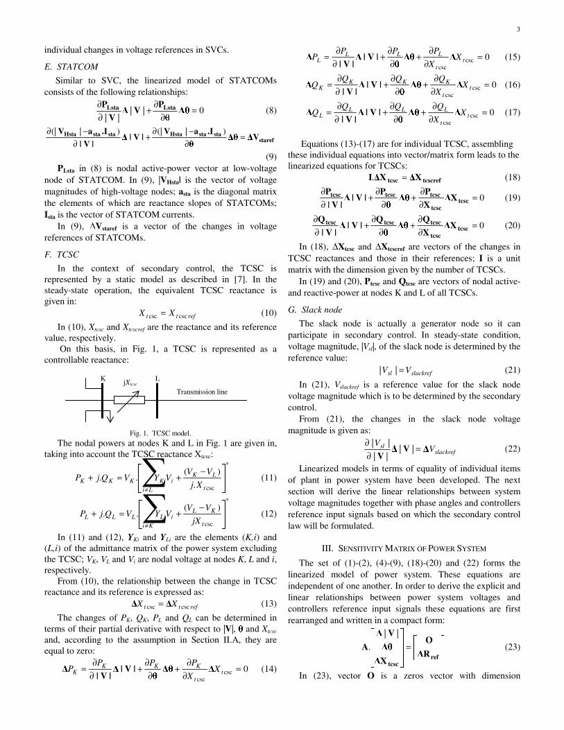
3
individual changes in voltage references in SVCs.
E. STATCOM
Similar to SVC, the linearized model of STATCOMs consists of the following relationships:
0||||
=∂
∂+∂∂
∆θθ
PV∆
VP LstaLsta (8)
starefstastaHstastastaHsta
∆V∆θθ
.IaV|V|∆
|V|
.IaV=
∂−∂
+∂
−∂ )|(|)|(|
(9) PLsta in (8) is nodal active-power vector at low-voltage
node of STATCOM. In (9), |VHsta| is the vector of voltage magnitudes of high-voltage nodes; asta is the diagonal matrix the elements of which are reactance slopes of STATCOMs; Ista is the vector of STATCOM currents.
In (9), ∆Vstaref is a vector of the changes in voltage references of STATCOMs.
F. TCSC
In the context of secondary control, the TCSC is represented by a static model as described in [7]. In the steady-state operation, the equivalent TCSC reactance is given in:
reftt XX csccsc = (10)
In (10), Xtcsc and Xtcscref are the reactance and its reference value, respectively.
On this basis, in Fig. 1, a TCSC is represented as a controllable reactance:
Fig. 1. TCSC model.
The nodal powers at nodes K and L in Fig. 1 are given in, taking into account the TCSC reactance Xtcsc:
*
csc.
)(..
⎥⎥⎦
⎤
⎢⎢⎣
⎡ −+=+ ∑
≠ t
LK
LiiKiKKK Xj
VVVYVQjP (11)
*
csc
)(..
⎥⎥⎦
⎤
⎢⎢⎣
⎡ −+=+ ∑
≠ t
KL
KiiLiLLL jX
VVVYVQjP (12)
In (11) and (12), YKi and YLi are the elements (K,i) and (L,i) of the admittance matrix of the power system excluding the TCSC; VK, VL and Vi are nodal voltage at nodes K, L and i, respectively.
From (10), the relationship between the change in TCSC reactance and its reference is expressed as:
reftt XX csccsc ∆∆ = (13)
The changes of PK, QK, PL and QL can be determined in terms of their partial derivative with respect to |V|, θ and Xtcsc and, according to the assumption in Section II.A, they are equal to zero:
0csccsc
=∂∂
+∂
∂+
∂∂
= tt
KKKK X
X
PPPP ∆∆θ
θ|V|∆
|V|∆ (14)
0csccsc
=∂
∂+
∂∂
+∂∂
= tt
LLLL X
X
PPPP ∆∆θ
θ|V|∆
|V|∆ (15)
0csccsc
=∂∂
+∂
∂+
∂∂
= tt
KKKK X
X
QQQQ ∆∆θ
θ|V|∆
|V|∆ (16)
0csccsc
=∂∂
+∂
∂+
∂∂
= tt
LLLL X
X
QQQQ ∆∆θ
θ|V|∆
|V|∆ (17)
Equations (13)-(17) are for individual TCSC, assembling
these individual equations into vector/matrix form leads to the linearized equations for TCSCs:
tcscreftcsc ∆X∆XI =. (18)
0=∂∂
+∂
∂+
∂∂
tcsctcsc
tcsctcsctcsc∆X
X
P∆θ
θ
P|V|∆
|V|
P (19)
0=∂∂
+∂
∂+
∂∂
tcsctcsc
tcsctcsctcsc∆X
X
Q∆θ
θ
Q|V|∆
|V|
Q (20)
In (18), ∆Xtcsc and ∆Xtcscref are vectors of the changes in TCSC reactances and those in their references; I is a unit matrix with the dimension given by the number of TCSCs.
In (19) and (20), Ptcsc and Qtcsc are vectors of nodal active- and reactive-power at nodes K and L of all TCSCs.
G. Slack node
The slack node is actually a generator node so it can participate in secondary control. In steady-state condition, voltage magnitude, |Vsl|, of the slack node is determined by the reference value:
slackrefsl VV =|| (21)
In (21), Vslackref is a reference value for the slack node voltage magnitude which is to be determined by the secondary control.
From (21), the changes in the slack node voltage magnitude is given as:
slackrefsl V
V∆V∆
V=
∂∂
||||
|| (22)
Linearized models in terms of equality of individual items of plant in power system have been developed. The next section will derive the linear relationships between system voltage magnitudes together with phase angles and controllers reference input signals based on which the secondary control law will be formulated.
III. SENSITIVITY MATRIX OF POWER SYSTEM
The set of (1)-(2), (4)-(9), (18)-(20) and (22) forms the linearized model of power system. These equations are independent of one another. In order to derive the explicit and linear relationships between power system voltages and controllers reference input signals these equations are first rearranged and written in a compact form:
⎥⎦
⎤⎢⎣
⎡=
⎥⎥⎥
⎦
⎤
⎢⎢⎢
⎣
⎡
reftcsc
∆R
O
∆X
∆θ
V∆
A
||
. (23)
In (23), vector O is a zeros vector with dimension
K L
Transmission line jXtcsc

4
determined by the number of load nodes excluding TCSC nodes, nload, number of generators, ngen number of SVCs, nsvc, number of STATCOMs, nsta, and number of TCSCs, ntcsc. Dimension of O is (2nload + ngen + nsvc + nsta + 4ntcsc). ∆Rref in (23) is the vector of the changes in reference input
signals to controllers, the dimension of which is given by the number of generators including the slack node generator, ngen+1, number of SVCs, STATCOMs and TCSCs. Dimension of ∆Rref is (ngen+nsvc+nsta+ntcsc+1):
⎥⎥⎥⎥⎥⎥
⎦
⎤
⎢⎢⎢⎢⎢⎢
⎣
⎡
=
tcscref
staref
svcref
genref
ref
∆X
∆V
∆V
∆V
∆
∆R
slackrefV
(24)
In (23), matrix A is defined as:
⎥⎥⎥⎥⎥⎥⎥⎥⎥⎥⎥⎥⎥⎥⎥⎥⎥⎥⎥⎥⎥⎥⎥⎥⎥⎥⎥⎥⎥⎥⎥⎥⎥
⎦
⎤
⎢⎢⎢⎢⎢⎢⎢⎢⎢⎢⎢⎢⎢⎢⎢⎢⎢⎢⎢⎢⎢⎢⎢⎢⎢⎢⎢⎢⎢⎢⎢⎢⎢
⎣
⎡
∂∂
∂−∂
∂−∂
∂−∂
∂∂
∂∂
∂∂
∂∂
∂∂
∂∂
∂∂
∂∂
∂∂
∂∂
∂∂
∂∂
∂∂
∂∂
∂∂
∂∂
∂∂
∂∂
=
I
θ
V
|V|
.IaVθ
.IaV|V|
.IaVV
VV
XQ
θ
Q|V|
QXP
θ
P|V|
Pθ
P
V
Pθ
PV
Pθ
P
V
Pθ
QV
Qθ
P
V
P
A
stastastaHsta
svcsvcHsvcsvcsvcHsvc
gen
tcsc
tcsctcsctcsc
tcsc
tcsctcsctcsc
LstaLsta
LsvcLsvc
gengen
loadload
loadload
00
0)|(|
0)|(|)|(|
00||
||
00||
||
0||
0||
0||
0||
0||
slV
(25) Matrix A is calculated at the current operating condition of
the power system, (|V0|, θ0), and the current values of TCSCs reactances. Dimension of matrix A is dependent on the number of power system nodes, nnode, which is determined as:
12 csc +++++= tstasvcgenloadnode nnnnnn (26)
Dimension of matrix A is (2nnode+ntcsc-1)x(2nnode+ntcsc-1).
Dimension of vector
⎥⎥⎥
⎦
⎤
⎢⎢⎢
⎣
⎡
tcsc∆X
∆θ
V∆ ||
is (2nnode+ntcsc-1).
Solving the system of linear equations in (23) gives:
⎥⎦
⎤⎢⎣
⎡=
⎥⎥⎥
⎦
⎤
⎢⎢⎢
⎣
⎡−
reftcsc
∆R
OA
∆X
∆θ
V∆
.
||1 (27)
As matrix A is highly sparse, a sparsity scheme based on LU factorization is used to form the elements of A-1. This is more efficient and faster than directly forming the inverse of A by a standard matrix inversion routine.
In order to eliminate unnecessary elements in matrix A-1, and at the same time to form separate equations related to ∆|V|, ∆θ and ∆Xtcsc, matrix A-1 is partitioned as shown in (28) into appropriate submatrices B, Cv, Cθ and Cx with dimensions as follows:
Dimension of B is determined based on those of matrix A and O: (2nnode+ntcsc-1)x(2nload+ngen+nsvc+nsta+4ntcsc).
Dimension of Cv is determined based on the number of node and controllers: nnodex(ngen+nsvc+nsta+ntcsc+1).
Dimension of Cθ is determined based on the number of node less 1 and controllers: (nnode-1)x(ngen+nsvc+nsta+ntcsc+1).
Dimension of Cx is determined based on the number of TCSCs and that of controllers: ntcscx(ngen+nsvc+nsta+ntcsc+1).
⎥⎥⎥⎥⎥⎥
⎦
⎤
⎢⎢⎢⎢⎢⎢
⎣
⎡
=−
x
θ
v
1
C
CB
C
A
M
KM
M
LM
M
(28)
Substituting (28) into (27) gives:
refv ∆RCV∆ .|| = (29)
refθ∆RC∆θ .= (30)
refxtcsc ∆RC∆X .= (31)
Equations (29)-(31) give linear and explicit relationships between the changes in the system voltage magnitudes, phase angles as well as in the TCSC reactances and those in the reference values of the controllers. In order to develop a strategy for secondary control to achieve a minimum active-power loss, it is necessary to derive the relationships between the controlled quantities and the controller reference values.
IV. CONTROLLED QUANTITIES SENSITIVITIES
In steady-state operation, there are always the active- and reactive-power balances. Minimizing the active-power loss is therefore equivalent to minimizing the slack node active-power. Active-power at slack node, Psl, is expressed as:
[ ]⎭⎬⎫
⎩⎨⎧= ∑
*, .Re iislslsl VYVP (32)
where Ysl,i is the element (sl,i) of the admittance matrix of the power system.
From (32), the change of slack node active-power which is also the change of active-power loss is determined and has the form:
∆θθ
|V|∆V
∆∂
∂+∂∂= slsl
lossPP
P||
(33)
or ⎥⎦
⎤⎢⎣
⎡⎥⎦
⎤⎢⎣
⎡
∂∂
∂∂
=∆θ
|V|∆
θV∆
slslloss
PPP
|| (34)
Substituting (29) and (30) into (34) yields:

5
refPloss R.∆C∆ =lossP (35)
where ⎥⎦
⎤⎢⎣
⎡⎥⎦
⎤⎢⎣
⎡
∂∂
∂∂=
θ
vPloss C
C
θVC slsl PP
|| (36)
In the secondary control, another objective is to maintain the security of the power system when a contingency condition occurs. The controller reference values are determined to minimize active-power loss, subject to the constraints that all controllers operating quantities, nodal voltage magnitudes and branch power flows are within their limits.
The relationship between the changes in operating quantities which are generator reactive-power, SVC susceptance, STATCOM current and TCSC reactance, and their reference values are first developed.
From [5], the changes in reactive-power of generators can be expressed in a linearized form as follows:
∆θθ
Q|V|∆
|V|
Q∆Q gengen
gen ∂∂
+∂∂
= (37)
Substituting (29) and (30) in (37) gives:
refQgengen ∆RC∆Q .= (38)
where ⎥⎦
⎤⎢⎣
⎡⎥⎦
⎤⎢⎣
⎡
∂∂
∂∂
=θ
vgengenQgen C
C
θ
Q
V
QC
|| (39)
SVC susceptance change is given in a linearized form [5]:
∆θθ
B|V|∆
|V|B
∆B svcsvcsvc ∂
∂+∂∂= (40)
Substituting (29) and (30) in (40) gives:
refBsvcsvc R.∆C∆B = (41)
where ⎥⎦
⎤⎢⎣
⎡⎥⎦
⎤⎢⎣
⎡
∂∂
∂∂=
θ
vsvcsvcBsvc C
C
θ
B|V|
BC (42)
STATCOM current change in linearized form is given [5]:
∆θ|θ|
I|V|∆
|V|I
∆I stastasta ∂
∂+∂∂= (43)
Substituting (29) and (30) in (43) gives:
refIstasta R.∆C∆I = (44)
where ⎥⎦
⎤⎢⎣
⎡⎥⎦
⎤⎢⎣
⎡
∂∂
∂∂=
θ
vstastaIsta C
C
θ
I|V|
IC (45)
Limits of each TCSC in steady-state condition are in terms of reactance. The changes in TCSCs reactances have been derived in (31).
Equations (38), (41), (44) and (31) give the linearised relationships between the changes in operating quantities of controllers such as generators, SVCs, STATCOMs and TCSCs, and those in controllers references. The following is developed the relationship between the changes in branch power flows and those in controller references.
Apparent power flow at one end in a branch is determined by active- and reactive-power flows:
22SSS QPS += (46)
22RRR QPS += (47)
In (46) and (47), SS and SR are apparent power flows at the sending end and receiving end, respectively.
PS and QS, and PR and QR in (46) and (47) are active- and reactive-power flows at the sending end and receiving end of the branch, respectively, which are functions of voltage magnitudes and phase angles at the two ends of the branch.
The changes in apparent power flows at the sending end and the receiving end can be expressed as:
∆θθ
|V|∆V
∆∂
∂+∂∂= SS
SSS
S||
(48)
∆θθ
|V|∆V
∆∂
∂+∂∂= RR
RSS
S||
(49)
Equations (48) and (49) are rewritten in a vector/matrix form:
⎥⎦
⎤⎢⎣
⎡⎥⎦
⎤⎢⎣
⎡
∂∂
∂∂
=∆θ
|V|∆
θV∆
SSS
SSS
|| (50)
⎥⎦
⎤⎢⎣
⎡⎥⎦
⎤⎢⎣
⎡
∂∂
∂∂
=∆θ
|V|∆
θV∆
RRR
SSS
|| (51)
Extending (50) and (52) for all branches in power system gives the change in branch apparent power flows in vector/matrix form:
⎥⎦
⎤⎢⎣
⎡⎥⎦
⎤⎢⎣
⎡
∂∂
∂∂
=∆θ
|V|∆
θ
SV
S∆S bSbS
bS || (52)
⎥⎦
⎤⎢⎣
⎡⎥⎦
⎤⎢⎣
⎡
∂∂
∂∂=
∆θ
|V|∆
θ
SV
S∆S bRbR
bR || (53)
In (52) and (53), ∆SbS and ∆SbR are vectors of apparent power flow changes at the sending end and receiving end, respectively, in all branches.
Substituting (29) and (30) into (52) and (53) yields: refSbSbS R∆C∆S .= (54)
refSbRbR R∆C∆S .= (55)
where ⎥⎦
⎤⎢⎣
⎡⎥⎦
⎤⎢⎣
⎡
∂∂
∂∂=
θ
VbSbSSbS C
C
θ
SV
SC
|| (56)
⎥⎦
⎤⎢⎣
⎡⎥⎦
⎤⎢⎣
⎡
∂∂
∂∂=
θ
VbRbRSbR C
C
θ
SV
SC
|| (57)
V. CONTROL STRATEGY
The objective of the secondary control in the paper is to determine the optimal set of controllers references to minimize the active-power loss. An objective function is formed using (35):
refPloss R.∆C=F (58)
The objective function F in (58) is minimized with respect to ∆Rref subject to inequality constraints related to limits on system voltage magnitudes, generator reactive-powers, SVCs susceptances, STATCOMs operating currents, TCSC reactances and branch power flows. The set of inequality constraints are as follows:
maxrefvmin ∆V∆RC∆V ≤≤ . (59)
genmaxrefQgengenmin ∆Q∆RC∆Q ≤≤ . (60)

6
svcmaxrefBsvcsvcmin ∆BR.∆C∆B ≤≤ (61)
stamaxrefIstastamin ∆IR.∆C∆I ≤≤ (62)
tcscmaxrefxtcscmin ∆XR.∆C∆X ≤≤ (63)
max. brefSbS ∆S∆RC ≤ (64)
max. brefSbR ∆S∆RC ≤ (65)
In (59), ∆Vmin and ∆Vmax are vectors of deviations between the allowable minimum and maximum voltage magnitudes at all nodes and the current operating voltage magnitudes at these nodes, respectively.
In (60), ∆Qgenmin and ∆Qgenmax are vectors of the differences between the minimum and maximum reactive-power limits of generators and their current operating reactive-powers, respectively.
In (61), ∆Bsvcmin and ∆Bsvcmax are vectors of the differences between the inductive limits and capacitive limits of SVCs and their current operating susceptances, respectively.
In (62), ∆Istamin and ∆Istamax are vectors of the differences between the minimum and maximum current limits of STATCOMs and their operating currents, respectively.
In (63), ∆Xtcscmin and ∆Xtcscmax are vectors of the differences between the minimum and maximum reactance limits of TCSCs and their current operating reactance, respectively.
In (64) and (65), ∆Sbmax is vector of the differences between the maximum power flow limits of all branches and their current operating apparent power flow.
In the above, the secondary control strategy is expressed as a linear programming problem. Efficient and robust methods for solving such a problem have been well developed and available in MATLAB environment.
The dimension of the vector of control variables in the optimization is relatively low in comparison with the number of power network nodes.
The optimal solution provided by the optimization, ∆Rref, augments the current vector of controllers reference settings, R0
ref, to give the new ones:
refrefref ∆RRR += 0 (66)
VI. SECONDARY CONTROL RANGE EXTENSION
The secondary control strategy based on linearized system model in Section V is valid when the changes, as a result of the control, from the current operating point of the controlled quantities which are nodal voltage magnitudes and branch power flows are small. However, at the current operating point, if the values of the controlled quantities exceed their operating limits by significant extents, the solution obtained from the control strategy does not necessarily lead to desirable power system responses which restore the security.
In this case, the overall control strategy is sub-divided into a number of stages. Each stage requires the solution of the LP problem of the form given in Section V. In each stage, the allowable changes of the controlled quantities are limited to the ranges within which the linearized power system model is applicable. The lower and upper limits of the changes in the
controlled quantities for the LP problem are set, based on the valid ranges. The solution obtained from solving the LP problem in each stage will then be a valid one.
After each stage, a full power-flow analysis is carried out, using the controllers reference inputs obtained from the LP solution at that stage. This gives a revised operating point from which the coefficient matrices in (58)-(65) are recalculated, using the linearization procedure described in Sections II-IV. The revised LP problem for the next stage is then defined with the limits on the changes in the controlled quantities to be formed from the revised operating point and the valid range. The LP problem is then solved. The sequence is applied iteratively until the final stage. In this way, in the final stage, the differences between the controlled quantities at the current operating point and their required operating limits are within the valid range, and the final LP problem is formulated, with the limits on the changes in the controlled quantities are set to be the differences.
Extensive simulation studies have been performed to estimate the valid ranges of controlled quantity variations for which the linearized power system model is applicable. The study results indicate that the linearized model is valid if the variations are limited to about 5% of the controlled quantities relative to their values at the current operating point. The number of stages required in the secondary control therefore depends on the extent of the operating limit violation at the initial operating point defined from the information received from the PMUs and/or state estimation.
VII. SECONDARY CONTROL LOOP
Following the static security assessment, corrective control measures will be required if there are any violations of nodal voltage limits and/or branch power flows. The control measures for restoring system security are provided by power systems controllers which include generator excitation controllers and FACTS devices. The secondary control scheme proposed offers this control function by which optimal reference inputs to the controllers are determined online. The scheme can be implemented as a software module within the Energy Management System (EMS) as shown in Fig. 2. The module draws the information obtained the PMUs and other functions in the EMS which include state estimation, and power system configuration determination. The outputs from the secondary control module are the reference input signals required by the controllers.
Fig. 2. Scheme of the secondary voltage control.
Rref
CONTROL CO-ORDINATION
PMUs and/or STATE
ESTIMATION
POWER SYSTEM
DATABASE
CIRCUIT-BREAKERS
and ISOLATORS STATUSES
POWER SYSTEM
POWER SYSTEM CONFIGURATION DETERMINATION

7
VIII. SIMULATION RESULTS
A. System Configuration
This section presents the simulation results carried out using a representative power system with 330 kV transmission lines which is shown in Fig. 3.
Fig. 3. Configuration of 10-node power system.
Compensation measures based on an SVC at node 3, a STATCOM at node 4 and two TCSCs in the transmission lines identified by A and B in Fig. 3 are installed to increase the transmission system power transfer capability required for supplying load demands. Reference settings of the controllers are given in Table 1.
TABLE I CONTROLLER REFERENCE SETTINGS
Controller Reference setting (pu) Generator 1 1.050 Generator 2 1.050
SVC 1.076 STATCOM 1.070
TCSC 1 -0.0846 TCSC 2 -0.1000
pu on 100 MVA base
In Table I, generator 1 and generator 2 are those at nodes 1 and 2, respectively; TCSC1 and TCSC2 are those in transmissions lines A and B, respectively.
By standard load-flow analysis, the current operating point of the power system for a given load demand and generation schedule together with the system configuration is obtained. In the following section, the case study in relation to secondary control subsequent to the disturbance of a large load demand increase will be carried out.
B. Case Study
In this case, load demand at node 6 increases significantly to 500+j250 MVA. This results in the considerable decrease in voltage magnitudes at nodes 5 (0.920 pu) and 6 (0.919 pu), the overload in transmission line between nodes 2 and 4 (724.0 MVA in comparison with its limit of 650.0 MVA). Due to the unacceptable voltage profile and transmission line
overload, the secondary control is invoked. New set of reference settings is optimally determined by the control to minimize active-power loss, improve voltage profile and alleviate transmission overloading. New optimal reference settings and active-power loss are given in Table II.
TABLE II
CONTROLLER REFERENCE SETTINGS AND ACTIVE-POWER LOSS BEFORE AND
AFTER RESPONSE OF SECONDARY CONTROL
Secondary control Before After Generator 1 voltage 1.050 1.050 Generator 2 voltage 1.050 1.050 SVC voltage 1.076 1.071 STATCOM voltage 1.070 1.034 TCSC 1 reactance -0.0846 -0.1068
Controller references
setting (pu)
TCSC 2 reactance -0.1000 -0.1018 Active-power loss (MW) 145 142
In Fig. 4 are given voltage profiles after the change in load demand at node 6 as well as the voltage profile after the response of the secondary control.
1 2 3 4 5 6 0.7 0.75 0.8
0.85 0.9
0.95 1
1.05 1.1
node
volta
ge m
agni
tude
(pu
)
Fig. 4. System voltage profile.
___ Normal condition --- Increase in load demand … After the response of secondary control
Apparent power flow in the transmission line between nodes 2 and 4 is 650.0 MVA which is at the limit value.
IX. CONCLUSION
The secondary control scheme which has been successfully developed in the paper addresses some of the key requirements related to corrective measures for restoring system security following system disturbance/contingency. The scheme proposed provides the optimal adjustments of power system controllers reference settings in a co-ordinated manner to satisfy system operating constraints in terms of voltages and power flows, and achieve at the same time minimum network loss. The scheme helps system operators avoid the use of preventative control measures in economic dispatch. This will further lower the overall operating cost, which is an important issue in the new electricity market environment.
Given the widespread availability of PMUs and increasing application of FACTS devices, at present, it is feasible to
6
TCSC
TCSC
SVC
STATCOM
1 3 5
2 4
9
10
7
8
400+j194
(MVA) 500+j242
(MVA)
300+j145
(MVA) 200+j97
(MVA)
1000 MW
A
B

8
implement and apply the scheme within the EMS environment.
The accuracy and robustness of the scheme have been verified with many simulation studies of a range of power system configurations and operating conditions. Full power-flow analyses have been used to validate the responses output from the proposed secondary control scheme.
X. ACKNOWLEDGMENT
The authors gratefully acknowledge the support of the Energy Systems Centre at The University of Western Australia for the research work reported in the paper. They express their appreciation to The University of Western Australia for permission to publish the paper.
XI. REFERENCES [1] J.P. Paul, J.Y. Leost, and J.M. Tesseron, “Survey of the secondary voltage
control in France: present realization and investigations,” IEEE Trans. Power Systems, vol. 2, no. 2, pp. 505-511, May 1987.
[2] A. Stankovie, M. Elic, and D. Maratukulam, “Recent results in secondary voltage control of power systems,” IEEE/PES 1990 Winter Meeting, Atlanta, Georgia, , pp.94-101, 1990.
[3] B. Marinescu, and H. Bourles, “Robust predictive control for the flexible coordinated secondary voltage control of large-scale power systems,” IEEE Trans. Power Systems, vol. 14, no. 4, pp. 1262-1268, 1999.
[4] H. F. Wang, H. Li, and H. Chen, “Coordinated secondary voltage control to eliminate voltage violations in power system contingencies,” IEEE Trans. Power Systems, vol. 18, no. 2, pp. 588-595, May 2003.
[5] T.T. Nguyen and V.L. Nguyen, “Application of wide-area network of phasor measurements for secondary voltage control in power systems with FACTS controllers,” in Proc. 2006 IEEE Power Engineering Society General Meeting, pp. 1669-1676.
[6] B. Stott, O. Alsac, and A. J. Monticelli, “Security analysis and optimization,” IEEE Proceedings, vol. 75, no. 12, pp. 1623-1644, 1987.
[7] CIGRE TF 38.01.08: “Modeling of power electronics equipment (FACTS) in load flow and stability programs: a representation guide for power system planning and analysis,” 1998.
XII. BIOGRAPHIES
T.T. Nguyen was born in Saigon, Vietnam, in 1956. Currently, he is an Associate Professor at The University of Western Australia. He was an invited lecturer in power system short courses in Thailand and Indonesia (1985), the Philippines (1986), Malaysia (1986, 1990), Singapore (1992), Vietnam (1999, 2000, 2003) and in the inaugural course (1991) in the national series of short course in power systems sponsored by the Electricity Supply Association of Australia (ESAA). He was the
Director of the ESAA 2000 Residential School in Electric Power Engineering. His interests include power systems modeling, analysis and design; power systems control and protection, quality of supply, transmission asset management and applications of neural networks and wavelet networks in power systems. He has published more than 100 papers in international literature, three undergraduate textbooks, and four short course textbooks. Professor Nguyen was awarded the Sir John Madsen Medal of the Institution of Engineers, Australia in 1981 and 1990. He serves on CIGRE International Task Forces. He was the Chairman of the Australasian Universities Power Engineering Conference in 1995.
V.L. Nguyen (Student member, IEEE) was born in Ho Chi Minh City, Vietnam, in 1964. He received his BE in Electrical Engineering from Ho Chi Minh City University of Technology in 1986. Since then, he was appointed as an Associate Lecturer and then promoted to Lecturer in the same University. He is currently a PhD student under the supervision of Associate Professor T.T. Nguyen at the Energy Systems Centre, The University of Western Australia. His research interests are in the fields of power systems modeling, analysis
and control with particular reference to stability and FACTS.

______________________________________________________________________
244
Bibliography
[1] Tomsovic, K., Bakken, D.E., Venkatasubramanian, V., and Bose, A.: ‘Designing
the next generation of real-time control, communication, and computations for
large power systems’, Proceedings of IEEE, 2005, 93, (5), pp. 965 – 979
[2] Noroozian, M., Andersson, G., and Tomsovic, K.: ‘Robust, near time-optimal
control of power system oscillations with fuzzy logic’, IEEE Trans. Power
Deliv., 1996, 11, (1), pp. 393 – 400
[3] Ni, H., Heydt, G.T., and Mili, L.: ‘Power system stability agents using robust
wide area control’, IEEE Trans. Power Syst., 2002, 17, (4), pp. 1123 – 1131
[4] Wu, H., Tsakalis, K.S., and Heydt, G.T.: ‘Evaluation of time delay effects to
wide-area power system stabilizer design’, IEEE Trans. Power Syst., 2004, 19,
(4), pp. 1935 – 1941
[5] Majumder, R., Chaudhuri, B., and Pal, B.C.: ‘Implementation and test results of
a wide-area measurement-based controller for damping interarea oscillations
considering signal-transmission delay’, IET Gener. Transm. Distrib., 2007, 1,
(1), pp. 1 – 7
[6] Korba, P., Larsson, M., Chaudhuri, B., Pal, B., Majumder, R., Sadikovic, S.,
and Andersson, G.: ‘Toward real-time implementation of adaptive damping
controllers for FACTS devices’, Proc. IEEE PES General Meeting, Florida,
USA, June 2007
[7] Nguyen, T.T. and Gianto, R.: ‘Neural networks for adaptive control coordination
of PSSs and FACTS devices in multimachine power system’, IET Gener.
Transm. Distrib., 2008, 2, (3), pp. 355 – 372

______________________________________________________________________
245
[8] Athay, T.N.: ‘Generation scheduling and control’, Proceedings of IEEE, 1987,
75, (12), pp. 1592 – 1606
[9] Christie, R.D. and Bose, A.: ‘Load frequency control issues in power system
operations after deregulation’, IEEE Trans. Power Syst., 1996, 11, (3), pp. 1191
– 1200
[10] Bhowmik, S., Tomsovic, K. and Bose, A.: ‘Communication models for third
party load frequency control’, IEEE Trans. Power Syst., 2004, 19, (1), pp. 543 –
548
[11] Yu, X. and Tomsovic, K.: ‘Application of linear matrix inequalities for load
frequency control with communication delays’, IEEE Trans. Power Syst., 2004,
19, (3), pp. 1508 – 1515
[12] Gotham, D. and Heydt, G.T.: ‘Power flow control and power flow studies for
systems with FACTS devices’, IEEE Trans. Power Syst., 1998, 13, (1), pp. 60 –
65
[13] Tomsovic, K.: ‘A fuzzy linear programming approach to the reactive
power/voltage control problem’, IEEE Trans. Power Syst., 1992, 7, (1), pp. 287
– 293
[14] Paul, J.P., Leost, J.Y., and Tesseron, J.M.: ‘Survey of the secondary voltage
control in France: present realization and investigations’, IEEE Trans. Power
Syst., 1987, 2, (2), pp. 505 – 511
[15] Le, T.L., Negnevitsky, M. and Piekutowski, M.: ‘Network equivalents and
expert system application for voltage and VAR control in large-scale power
systems’, IEEE Trans. Power Syst., 1997, 12, (4), pp. 1440 – 1445
[16] Stott, B., Alsac, O., and Monticelli, A. J.: ‘Security analysis and optimization’,
Proceedings of IEEE, 1987, 75, (12), pp. 1623 – 1644
[17] Mehraban, A.S., Edris, A., Schauder, C.D., Provanzana, J.H.: ‘Installation,
commissioning, and operation of the world’s first UPFC on the AEP system’,
Proceedings POWERCON’98, 1998, 1, pp. 323 – 327
[18] Schauder, C.D., Gyugyi, L., Lund, M.R., Hamai, D.M., Rietman, T.R.,
Torgerson, D.R., and Edris, A.: ‘Operation of the unified power flow controller
(UPFC) under practical constraints’, IEEE Trans. Power Deliv., 1998, 13, (2),
pp. 630 – 639

______________________________________________________________________
246
[19] Vu, H., Pruvot, P., Launay, C., and Harmand, Y.: ‘An improved voltage control
on large-scale power system’, IEEE Trans. Power Syst., 1996, 11, (3), pp. 1295
– 1303
[20] Corsi, S., Marannino, P., Losignore, N. Moreschini, G., and Piccini, G.:
‘Coordination between the reactive power scheduling function and the
hierarchical voltage control of the EHV ENEL system’, IEEE Trans. Power
Syst., 1995, 102, (2), pp. 686 – 694
[21] Sancha, J.L., Fernadez, J.L., Cortes, A., and Abarca, J.T.: ‘Secondary voltage
control: Analysis, solution and simulation results for the Spanish transmission
system’, IEEE Trans. Power Syst., 1996, 11, (2), pp. 630 – 638
[22] Van Hecke, J., Janssens, N., Deuse, J., and Promel, F.: ‘Coordinated voltage
control experience in Belgium’, Cigre report, Paris, France, August 2000, pp. 38
– 111
[23] Taranto, G.N., Martins, N., Falcao, D.M., Martins, A.C.B., and dos Santos,
M.G.: ‘Benefits of applying secondary voltage control schemes to the Brazilian
system’, Proc. IEEE PES Summer Meeting, Seattle, Washington, USA, July
2000, vol. 2, pp. 937 – 942
[24] Hingorani, N.G.: ‘FACTS – Flexible AC transmission system’, Proc. IEE Fifth
Int. Conf. AC and DC Power transmission, London, UK, September 1991, pp. 1
– 7
[25] Edris, A., and task Force members: ‘Proposed term and definitions for flexible
AC transmission system (FACTS)’, IEEE Trans. Power Deliv., 1997, 12, (4),
pp. 1848 – 1853
[26] Gyugyi, L.: ‘Power electronics in electric utilities: Static Var compensators’,
Proc. IEEE, 1988, 76, (4), pp. 483 – 494
[27] ‘Modelling of Power Electronics Equipment (FACTS) in Load Flow and
Stability Programs: a Representation Guide for Power System Planning and
Analysis’. Task Force 38.01.08; Cigre, 1999
[28] Nguyen, T.T., and Nguyen, V.L.: ‘Application of wide-area network of phasor
measurements for secondary voltage control in power systems with FACTS
controllers’, Proc. IEEE PES General Meeting, San Francisco, USA, June 2005,
3, pp. 2927 – 2934
[29] Hingorani, N.G. and Gyugyi, L.: Understanding FACTS: Concepts and
technology of flexible AC transmission systems, IEEE Press, USA, 1999

______________________________________________________________________
247
[30] Mathur, R.M, and Varma, R.K.: Thyristor-based FACTS controllers for
electrical transmission system, IEEE Press, USA, 2002
[31] Larsen, E.V., Clark, K., Miske, S.A., Urbanek, J.: ‘Characteristic and rating
considerations of thyristor controlled series compensation’, IEEE Trans. Power
Deliv., 1994, 9, (2), pp. 992 – 1000
[32] Nguyen, T.T., and Nguyen, V.L.: ‘Power system security restoration by
secondary control’, Proc. IEEE PES General Meeting, Florida, USA, June 2007
[33] Yoshihiko, S., Yoshinobu, H., Hasegawa, T., et al.: ‘New static VAR control
using force-commutated inverters’, IEEE Trans. Power Appa. and Syst., 1981,
PAS-100, (9), pp. 4216 – 4224
[34] Edwards, C.W., Mattern, K.E., Stacey, E.J., Nannery, P.R., and Gubernick, J.:
‘Advanced state VAr generator employing GTO thyristors’, IEEE Trans. Power
Deliv., 1988, 3, (4), pp.1622 – 1627
[35] Ainsworth, J.D., Davies, M., Fitz, P.J., Owen, K.E., and Trainer, D.R.: ‘Static
Var compensator (STATCOM) based on single-phase chain circuit converters’,
IEE Proc. –Electr. Power Appl., 1998, 145, (4), pp. 381 – 386
[36] Schauder, C., Gemhardt, M., Stacey, E., Lemak, T., Gyugyi, L., Cease, T.W.,
and Edris, A.: ‘Development of a ± 100 MVAr static condenser for voltage
control of transmission systems’, IEEE Trans. Power Deliv., 1995, 10, (3), pp.
1486 – 1496
[37] Raju, N.R., Venkata, S.S., and Sastry, V.V: ‘The use of decoupled converters to
optimize the power electronic of shunt and series AC system controllers’, IEEE
Trans. Power Deliv., 1997, 12, (2), pp. 895 – 900
[38] Moran, L., Ziogas, P.D., and Joos, G.: ‘A Solid-state high-performance reactive-
power compensator’, IEEE Trans. Indus. Appl., 1993, 29, (5), pp. 969 – 978.
[39] Ooi, B.T., Dai, S.Z., and Wang, X.: ‘Solid-state series capacitive reactance
compensators’, IEEE Trans. Power Deliv., 1992, 7, (2), pp. 914 – 919
[40] Liu, Y.H., Arrillaga, J., and Watson, N.R.: ‘Multi-level voltage sourced
conversion by voltage reinjection at six times the fundamental frequency’, IEE
Proc. –Electr. Power Appl., 2002, 149, (3), pp. 201 – 207
[41] McGrath, B.P., and Holmes, D.G.: ‘Multicarrier PWM strategies for multilevel
inverters’, IEEE Trans. Industry Elec., 2002, 49, (4), pp.858 – 867

______________________________________________________________________
248
[42] Heydt, G.T.: ‘Power quality solution and their costs’, Proc. AUPEC 2005
Australian Universities Power Engineering Conference, September 2005, vol. 1,
pp. 1 – 8
[43] Heydt, G.T. and Suryanarayanan, S.: ‘Control strategies for electronic power
quality enhancement equipment’, Proc. AUPEC 2005 Australian Universities
Power Engineering Conference, September 2005, vol. 1, pp. 28 – 36
[44] Demiray, T. and Andersson, G.: ‘Comparison of the efficiency of dynamic
phasor models derived from abc to dq0 reference frame in power system
dynamic simulation’. Available from:
http://www.eech.ee.ethz.ch/downloads/psl/publications/TD-apscom2006.pdf
[45] Gyugyi, L.: ‘Unified power-flow control concept for flexible AC transmission
systems’ IEE Proc-C,1992, 139, (4), pp. 323 – 331
[46] Mohan, N., Undeland, and T.M., Robbins, W.P.: Power electronics: Converter,
application, and design, Second Edition, John Wiley & Sons, Inc., USA, 1995
[47] Bian, J., Ramey, D.G., Nelson, R.J., and Edris, A.: ‘A study of equipment sizes
and constraints for a unified power flow controller’, IEEE Trans. Power Deliv.,
1997, 12, (3), pp. 1385 – 11391
[48] Nabavi-Niaki, A., and Iravani, M. R.: ‘Steady-state and dynamic models of
unified power flow controller (UPFC) for power system studies’, IEEE Trans.
Power Syst., 1996, 11, (4), pp.1937 – 1943
[49] Fuerte-Esquivel, C.R., Acha, E.: ‘Unified power flow controller: a critical
comparison of Newton-Raphson UPFC algorithms in power flow studies’, IEE
Proc.-Gener. Trans. Distrib. 1997,144, (5), pp. 437 – 444
[50] Nguyen, T.T., and Nguyen, V.L.: ‘Representation of line optimisation control in
unified power flow controller model for power-flow analysis’, IET Gener.
Transm. Distrib., 2007, 1, (5), pp. 714 – 723
[51] Han, Z.X.: ‘Phase shifter and power flow control’, IEEE Trans. Power Appa.
Syst., 1982, 101, (10), pp. 3790 – 3795
[52] Noroozian, M., Angquist, L., Ghandhari, M., and Andersson, G.: ‘ Use of UPFC
for optimal power flow control’, IEEE Trans. on Power Delivery, 1997, 12, (4),
pp. 1629 – 1634
[53] Xiao, Y., Song, Y.H., and Sun, Y.Z.: ‘Power injection method and linear
programming for FACTS control’, Proc. IEEE PES Winter Meeting, Singapore,
Jan. 2000

______________________________________________________________________
249
[54] Liu, J. Y., Song, Y. H., and Foss A. M.: ‘ Strategies for handling UPFC
constraints in steady state power flow and voltage control’, IEEE Trans. on
Power Systems, 2000, 15, (2), pp.566 – 571
[55] Xiao, Y., Song, Y.H., and Sun, Y.Z.: ‘Power flow control approach to power
systems with embedded FACTS devices’, IEEE Trans. on Power Systems, 2002,
17, (4), pp. 943 – 950
[56] An, S., and Gedra, T.W.: ‘UPFC ideal transformer model’, Proceedings of North
Amer. Power Symp., 2003, pp.46 – 50
[57] An, S., Condren, J. and Gedra, T.W.: ‘An ideal transformer UPFC model, OPF
first-order sensitivities, and application to screening for optimal UPFC
locations’, IEEE Trans. on Power Syst, 2007, 22, (1), pp. 68 – 75
[58] Gyugyi, L., Schauder, C.D., Williams, S.L., Rietman, T.R., Torgerson, D.R., and
Edris, A.: ‘The unified power flow controller: A new approach to power
transmission control’, IEEE Trans. on Power Delivery, 1995, 10 (2), pp. 1085 –
1097
[59] ‘Application of optimisation techniques to study power system network
performance’. Task Force 38.04.02; Cigre,1997
[60] Bertsekas, D.P.: ‘Constrained optimization and Lagrange multiplier methods’
Academic Press, 1982
[61] Nino, E.E., Castro, C.A., da Silva, L.C.P., and Alves, D.A.: ‘Continuation load
flow using automatically determined branch megawatt losses as parameters’,
IEE Proc.-Gener. Transm. Distrib., 2006, 153, (3), pp. 300 – 308
[62] Ajjarapu, V., and Christy, C.: ‘The continuation power flow: A tool for steady
state voltage stability analysis’, IEEE Trans. Power Syst., 1992, 7, (1), pp. 416 –
423
[63] Chiang, H.D., Flueck, A.J., Shah, K.S., and Balu, N.: ‘CPFLOW: A practical
tool for tracing power system steady-state stationary behavior due to load and
generation variations’, IEEE Trans. Power Syst., 1995, 10, (2), pp. 623 – 634
[64] Brochu, J., Beauregard, F., Lemay, J., Morin, G., Pelletier, P., and Thallam,
R.S.: ‘Application of the interphase power controller technology for
transmission line power flow control’, IEEE Trans. Power Deliv., 1997, 12, (2),
pp. 888 – 894
[65] ‘Coordinated voltage control in transmission networks’. Task Force C4.602;
Cigre, 2007

______________________________________________________________________
250
[66] Lagonotte, P., Sabonnadiere, J.C., Leost, J.Y., and Paul, J.P.: ‘Structural analysis
of the electrical system: Application to secondary voltage control in France’,
IEEE Trans. Power Syst., 1989, 4, (2), pp. 479 – 486
[67] Lefebvre, H., Fragnier, D., Boussion, J.Y., Mallet, P., and Bulot, M.: ‘Secondary
coordinated voltage control system: Feedback of EDF’, Proc. IEEE PES
Summer Meeting, Seattle, Washington, USA, July 2000, vol. 1, pp. 290 – 295
[68] Arcidiacono, V., Corsi, S., and Marannino, P.: ‘The voltage and reactive control
of ENEL transmission system’, IEE Colloquium on International practices in
reactive power control, London, UK, April 1993
[69] Corsi S.: ‘The secondary voltage regulation in Italy’, Proc. IEEE PES Summer
Meeting, Seattle, Washington, USA, July 2000, vol. 1, pp. 296 – 304
[70] Janssens, N.: ‘Tertiary and secondary voltage control for the Belgian HV
system’, IEE Colloquium on International practices in reactive power control,
London, UK, April 1993
[71] Tesseron, J.M., Corsi, S., and Ashmole, P.H.: ‘Discussion of voltage scheme by
CEGB, ENEL, and EDF’, IEE Colloquium on CEGB/EDF/ENEL Collaboration
on Power System Planning and Operation, March 1988, pp. 2b/1 – 2b/26
[72] Ilic-Spong, M., Christensen, J., and Eichorn, K.L.: ‘Secondary voltage control
using pilot point information’, IEEE Trans. Power Syst, 1988, 3, (2), pp. 660 –
668
[73] Stankovie, A., Elic, M., and Maratukulam, D.: ‘Recent results in secondary
voltage control of power systems’, Proc. IEEE PES Winter Meeting, Atlanta,
Georgia, 1990, pp.94 – 101
[74] Conejo, A., Gomez, T., and de la Fuente, J.I.: ‘Pilot bus selection for secondary
voltage control’, European Transactions on Electrical Power Engineering, 1993,
vol. 3, (5), pp. 359 – 366
[75] Conejo, A., de la Fuente, J.I., and Goransson, S.: ‘Comparison of alternative
algorithms to select pilot buses for secondary voltage control in electric power
networks’, Proc. 7th Mediterranean Electrotechnical Conference, April 1994, vol.
3, pp. 940 – 943
[76] Conejo, A., and Aguilar, M.J.: ‘Secondary voltage control: Nonlinear selection
of pilot buses, design of an optimal control law, and simulation results’, IEE
Proc.-Gener. Transm. Distrib., 1998, 145, (1), pp. 77 – 81

______________________________________________________________________
251
[77] Wang, H. F., Li, H., and Chen, H.: ‘Coordinated secondary voltage control to
eliminate voltage violations in power system contingencies’, IEEE Trans. Power
Syst., 2003, 18, (2), pp. 588 – 595
[78] Kamwa, I., Grondin, R., and Hebert, Y.: ‘Wide-area measurement based
stabilizing control of large power systems – a decentralized/hierarchical
approach’, IEEE Trans. Power Syst., 2001,16, (1), pp. 136 – 153
[79] Heydt, G., Liu, C. Phake, A., and Vittal, V.: ‘Solution for the crisis in electric
power supply’, IEEE Trans. Power Syst., 2001,14, (3), pp. 22 – 30
[80] Milosevic, B., and Begovic, M.: ‘Voltage-stability protection and control using
a wide-area network of phasor measurements’, IEEE Trans. Power Syst.,
2003,18, (1), pp. 121 – 127
[81] ‘Wide area protection and emergency control’ (Final Report). Working Group
C-6, System Protection Subcommittee, IEEE PES Power System Relaying
Committee
[82] Humpage, W. D., Wong, K. P., and Nguyen, T. T.: ‘PROLOG network-graph
generation in system surveillance’, Electric Power System Research, 1985, no.9,
pp. 37 – 48
[83] Weedy, B.M. and Cory B.J.: Electric power systems, Fourth Edition, John Wiley
& Sons, Inc., UK, 1998
[84] Marinescu, B., and Bourles, H.: ‘Robust predictive control for the flexible
coordinated secondary voltage control of large-scale power systems’, IEEE
Trans. Power Syst., 1999, 14, (4), pp. 1262 – 1268
[85] Wen, J.Y., Wu, Q.H., Turner, D.R., Cheng, S.J., and Fitch, J.: ‘Optimal
coordinated voltage control for power system voltage stability’, IEEE Trans.
Power Syst., 2004, 19, (2), pp. 11115 – 122
[86] Alsac, O., Bright, J., Prais, M., and Stott, B.: ‘Further developments in LP-based
optimal power flow’, IEEE Trans. Power Syst., 1990, 5, (3), pp. 697 – 711
[87] Dandachi, N.H., Rawlins, M.J., Alsac, O., Prais, M., and Stott, B.: ‘OPF for
reactive pricing studies on the NGC system’, IEEE Trans. Power Syst., 1996,
11, (1), pp. 226 –232
[88] Tinney, W.F., Brandwajn, V., and Chan, S.M.: ‘Sparse vector methods’, IEEE
Trans. Power App. and Syst., 1985, PAS-104, (2), pp. 295 – 301
[89] Alvarado, F.L., Yu, D.C., and Betancourt, R.: ‘Partitioned sparse A-1 methods’,
IEEE Trans. Power Syst., 1990, 5, (2), pp. 452 – 459

______________________________________________________________________
252
[90] Latest flops.c results. Available from:
<http://gd.tuwien.ac.at/perf/benchmark/aburto/flops/flops_1.tbl>, <http://gd.tuwien.ac.at/perf/benchmark/aburto/flops/flops_2.tbl>, <http://gd.tuwien.ac.at/perf/benchmark/aburto/flops/flops_3.tbl> and <http://gd.tuwien.ac.at/perf/benchmark/aburto/flops/flops_4.tbl>
[91] Ristanovic, P., Bjelogrlic, M., and Bablic, B.S.: ‘Improvements in sparse
matrix/vector technique applications for on-line load flow calculation’, IEEE
Transactions on Power Systems, 1989, vol. 4, no. 1, pp. 190 – 196.

______________________________________________________________________
253
Appendices

______________________________________________________________________A.1
Appendix A STEADY-STATE MODEL FOR CONVENTIONAL POWER SYSTEM
ELEMENTS
Steady-state models for conventional power system elements including transmission
lines, series and shunt fixed compensators and transformers are presented in the present
appendix.
A.1 Overhead transmission lines and underground cable
In power system studies, both overhead lines and underground cables can be
characterised by four parameters which are distributed along the length of the line:
series resistance, series inductance, shunt conductance and shunt capacitance. It is
widely acknowledged that the transmission line can be modelled as an equivalent π
circuit given in Figure A.1:
Fig. A.1: Equivalent π circuit of a transmission line
In Fig. A.1, ZL and YL are the series impedance and shunt admittance of the transmission
line equivalent π circuit. They are determined using the following formulations:
)sinh(. lZZ cL γ= (A.1)
cL Z
l
Y)
2tanh(
γ
= (A.2)
In (A.1) and (A.2):
Zc is the characteristic impedance of the transmission line:
ZL
YL
s r
YL

______________________________________________________________________A.2
00
00
jBG
jXRZc +
+= (A.3)
γ is called the propagation constant:
))(( 0000 jBGjXR ++=γ (A.4)
In (A.3) and (A.4):
R0, X0, G0 and B0 are positive-phase-sequence resistance, reactance, conductance
and susceptance, respectively, of the transmission line in per unit length, and
l is the transmission line length.
If γl << 1, the expressions for ZL and YL in Fig. A.1 may be approximated as follows:
ljXRZL )( 00 += (A.5)
ljBG
YL )2
( 00 += (A.6)
The circuit model associated with this approximation is called the nominal π equivalent
circuit which can be applied for the following cases:
(i) l < 10000/f km for overhead line
(ii) l < 3000/f km for underground cable.
A.2 Series passive compensator
Series passive compensator is a lump element connecting in series with a transmission
line to compensate the electrical length of the line. The compensator, in steady-state
condition is considered as a branch between two nodes. Impedance form of series
passive compensators equivalent is given in Fig. A.2.
Fig. A.2: Impedance equivalent of series passive compensator
ZC a b

______________________________________________________________________A.3
A.3 Shunt passive compensator
Shunt passive compensator is a shunt branch connected to a node to perform reactive-
power compensation. The shunt passive compensator can be either a capacitor bank or a
reactor. A schematic representation of a shunt passive compensator is given in Fig. A.3.
Fig. A.3: Admittance equivalent of shunt passive compensator
A.4 Power transformer
Power transformers are used to connect sections of the network of different nominal
voltage. Almost always, power transformers are fitted with a tap-changing facility to
enable a degree of voltage magnitude control at one of the transformer terminals. Such
transformers are termed load tap-changing (LTC) transformers. The schematic
representation and equivalent circuit of a LTC transformer are given in Figs. A.4 and
A.5:
Fig. A.4: LTC transformer diagram
YC
n
T:1
ZT c d
c d TZ
T

______________________________________________________________________A.4
Fig. A.5: Admittance equivalent of LTC transformer
In Fig. A.4, ZT is the leakage impedance of the transformer and T is transformer voltage
ratio.
A.5 Power Network Nodal Admittance Matrix
A nodal admittance matrix of a power network is formed from the admittances of
branches which have been presented in the Sections A.1 – A.4 of the present appendix:
∑=i
Bkikk YY (A.7)
Bkiki YY −= (A.8)
In (A.7) and (A.8):
Ykk is the driving-point admittance element associated with node k;
Yki (for i ≠ k) is the transfer admittance element associated with nodes k and i;
YBkk is the admittance of the shunt branch connecting to node k, and
YBki (for i ≠ k) is the admittance of the branch connecting between nodes k and i.

______________________________________________________________________A.5
Appendix B POWER-FLOW EQUATIONS AND INEQUALITIES FOR INDIVIDUAL
NETWORK NODES
B.1 Load Node
Power-flow equations for load node loadk are given in terms of active- and reactive-
power mismatch equations:
0=− loadksploadk PP (B.1)
0=− loadksploadk QQ (B.2)
In (B.1) and (B.2):
Ploadksp and Qloadksp are specified values of active- and reactive-power of load node
loadk, and
Ploadk and Qloadk are nodal active- and reactive-power of load node loadk.
The expressions of Ploadk and Qloadk are given:
= ∑
iiiloadkloadkloadk VYVP *)..(Re , (B.3)
= ∑
iiiloadkloadkloadk VYVQ *)..(Im , (B.4)
In (B.3) and (B.4):
Vloadk and Vi are the nodal voltages at load node loadk and node i, and
Yloadk,i is element (loadk, i) of the nodal admittance matrix of the power network.
B.2. Generator node
Power-flow equations describing the steady-state model of the generator are given in the
following equations and inequalities:

______________________________________________________________________A.6
0=− genkspgenk PP (B.5)
0|| =− refgenkgenk VV (B.6)
0max ≤− genkgenk QQ (B.7)
0min ≤− genkgenk QQ (B.8)
In (B.5) – (B.8):
Pgenk and Pgenksp are the nodal active-power of generator at node genk and its
scheduled value;
|Vgenk| and Vrefgenk are the voltage magnitude at generator terminal and its reference
value, respectively, and
Qgenk, Qgenkmin and Qgenkmax are the reactive-power of generator at node genk and its
minimum and maximum allowable values, respectively.
Expressions of Pgenk and Qgenk are given as:
= ∑
iiigenkgenkgenk VYVP *)..(Re , (B.9)
= ∑
iiigenkgenkgenk VYVQ *)..(Im , B.10)
In (B.9) and (B.10):
Vgenk is the generator terminal voltage, and
Ygenk,i is element (genk, i) of the nodal admittance matrix of the power network.
B.3 SVC
The SVC steady-state model has been given in Section 2.3.2 of Chapter 2. In the
following are given the expressions of the nodal active-power at the SVC low-voltage
node, the SVC current and susceptance:
−
=svck
lsvckhsvcklsvcklsvck Z
VVVP
*).(Re
2
(B.11)

______________________________________________________________________A.7
−=
− )2
(.Re
hsvckj
svck
lsvckhsvcksvck e
Z
VVI
θπ
(B.12)
−−=
− )2
(.Re
||
1 hsvckj
svck
lsvckhsvck
hsvcksvck e
Z
VV
VB
θπ
(B.13)
In (B.11) – (B.13):
Plsvck is the nodal active-power at the SVC low-voltage node, lsvck;
Isvck is the SVC current;
Bsvck is the SVC susceptance;
Vhsvck and Vlsvck are the voltages at the low voltage node and high voltage node,
lsvck, of the SVC, respectively;
Zsvck is the leakage impedance of the SVC coupling transformer, and
θhsvck is the phase angle of the voltage at the SVC high voltage node.
B.4 STATCOM
In Section 2.3.4 has been presented the steady-state model of the STATCOM. The
following will give the expressions of the nodal active-power at the STATCOM low-
voltage node and the STATCOM current:
−
=stak
lstakhstaklstaklstak Z
VVVP
*).(Re
2
(B.14)
−=
− )2
(.Re
hstakj
stak
lstakhstakstak e
Z
VVI
θπ
(B.15)
In (B.14) – (B.15):
Plstak is the nodal active-power at the STATCOM low-voltage node, lstak;
Istak is the STATCOM current;
Zstak is the leakage impedance of the STATCOM coupling transformer;
θhstak is the phase angle of the voltage at the STATCOM high voltage node, hstak,
and

______________________________________________________________________A.8
Vhstak and Vlstak are the voltages at the low voltage node and high voltage node of the
STATCOM.
B.5 Generator transformer
Steady-state model of the generator-transformer set has been presented in Section10.3
of Chapter 10. The expressions of the nodal active- and reactive-power at the generator
terminal and the high voltage node of the generator transformer are given as:
−=
*2
ReT
hgengengengen Z
TVTVVP (B.16)
−=
*2
ImT
hgengengengen Z
TVTVVQ (B.17)
−= ∑
≠
*
,ReT
gen
geniiihgenhgenH Z
TVVYVP (B.18)
−= ∑
≠
*
,ImT
gen
geniiihgenhgenH Z
TVVYVQ (B.19)
In (B.16) – (B.19):
Pgen and Qgen are, respectively, nodal active- and reactive-power at the generator
node;
PH and QH are, respectively, nodal active- and reactive-power of the high voltage
node of the generator transformer;
Vgen and Vhgen are nodal voltages at generator node and the high voltage node of
the generator transformer, and
T is the voltage ratio of the generator transformer.
B.6 Transmission line power flow

______________________________________________________________________A.9
Power flows in the transmission line in Fig. A.1 are expressed in terms of the nodal
voltage at the sending- and receiving-end nodes as:
−+= *2)(
1)
1(Re rksk
Lksk
LkLksk VV
ZV
ZYP (B.20)
−+= *2)(
1)
1(Im rksk
Lksk
LkLksk VV
ZV
ZYQ (B.21)
−+= *2)(
1)
1(Re skrk
Lkrk
LkLkrk VV
ZV
ZYP (B.22)
−+= *2)(
1)
1(Im skrk
Lkrk
LkLkrk VV
ZV
ZYP (B.23)
In (B.20) – (B.23):
Psk and Qsk are active- and reactive-power in the transmission line between sending-
end node, sk, and receiving-end node, rk at the sending-end node;
Prk and Qrk are active- and reactive-power in the transmission line between the
sending- and receiving-end nodes, at the receiving-end node;
Vsk and Vrk are the nodal voltage at the sending- and receiving-end nodes at the
receiving-end node, and
ZLk and YLk are the series impedance and shunt admittance of the transmission line.

______________________________________________________________________A.10
Appendix C DATA FOR POWER SYSTEM USED IN CHAPTER 4
Table C.1: Transmission line data
No. Sending Node
Receiving Node
R (pu)
X (pu)
B (pu)
1 3 4 0.00338 0.02700 0.18217 2 4 5 0.00338 0.02700 0.18217 3 3 5 0.00338 0.02700 0.18217
Table C.2: Transformer data
No. Sending Node
Receiving Node
R (pu)
X (pu)
B (pu)
Off-nominal tap (%)
Vector Symbol
1 1 5 0.0 0.07 0 0 YY0 2 4 7 0.0 0.07 0 0 YY0
Table C.3: Load data
No. Node P
(MW) Q
(MVAr) 1 4 50 10 2 5 250 100
Table C.4: Generator data
No. Node |V|
(pu) P
(MW) Qmin
(MVAr) Qmax
(MVAr) 1 2 1.0 300 -100 180
Table C.5: Slack node
Node |V| P
(MW) Q
(MVAr) 1 1.00 0.0 0.0
Table C.6: Data for impedance of shunt and series converter transformers of
UPFC
Shunt Converter (pu) Series Converter (pu)
Resistance Reactance Resistance Reactance
0.0 0.03 0.0 0.03
Resistance, reactance and susceptance data is in pu on 100 MVA.

______________________________________________________________________A.11
Appendix D DATA FOR POWER SYSTEM USED IN CHAPTER 8
Table D.1: Transmission line data
No. Sending Node
Receiving Node
R (pu)
X (pu)
B (pu)
1 17 3 0.0024 0.0192 0.1298 2 17 4 0.0089 0.0720 0.4871 3 2 3 0.0020 0.0164 0.1109 4 2 5 0.0089 0.0720 0.4871 5 6 8 0.0597 0.1315 0.0291 6 6 10 0.0446 0.1003 0.0218 7 6 12 0.0325 0.0709 0.0157 8 7 11 0.0229 0.0504 0.0112 9 7 8 0.0597 0.1315 0.0291 10 8 9 0.0233 0.0514 0.0456 11 13 7 0.0266 0.0700 0.0148 12 14 10 0.0242 0.0540 0.0118 13 14 13 0.0309 0.0693 0.0151 14 14 15 0.0025 0.2000 0.0 15 15 11 0.0615 0.1620 0.0342 16 15 12 0.0040 0.0888 0.0197 17 16 4 0.0043 0.0351 0.2373 18 16 5 0.0043 0.0351 0.2373
Table D.2: Transformer data
No. Sending Node
Receiving Node
R (pu)
X (pu)
B (pu)
Off-nominal tap (%)
Vector Symbol
1 4 6 0.00230 0.0839 0.0 0 YY0 2 4 7 0.00185 0.1300 0.0 0 YY0 3 5 6 0.00230 0.0839 0.0 0 YY0 4 5 7 0.00230 0.0839 0.0 -5 YY0 5 17 22 0.0 0.0050 0.0 0 YD11 6 2 18 0.0 0.0060 0.0 0 YD11 7 16 1 0.0 0.0050 0.0 0 YD11 8 9 19 0.0 0.0700 0.0 0 YD11 9 14 20 0.0 0.0500 0.0 0 YD11 10 15 21 0.0 0.0550 0.0 0 YD11

______________________________________________________________________A.12
Table D.3: Load data
No. Node P
(MW) Q
(MVAr) 1 2 130 40 2 3 690 140 3 4 260 0 4 5 20 7 5 6 20 7 6 7 140 50 7 8 90 10 8 9 130 60 9 10 70 30 10 11 90 25 11 12 90 25 12 13 75 10 13 14 60 10 14 15 100 20 15 16 80 30 16 17 100 20
Table D.4: Generator data
No. Node |V| (pu)
P (MW)
Reactive-power limits (MVAr)
Absorption Supply 1 18 1.05 839 -250 500 2 19 1.05 200 -60 120 3 20 1.05 100 -30 60 4 21 1.05 180 -50 100 5 22 1.05 833 -250 500
Table D.5: Slack node
Node |V| P
(MW) Q
(MVAr) 1 1.00 0.0 0.0
Resistance, reactance and susceptance data is in pu on 100 MVA.
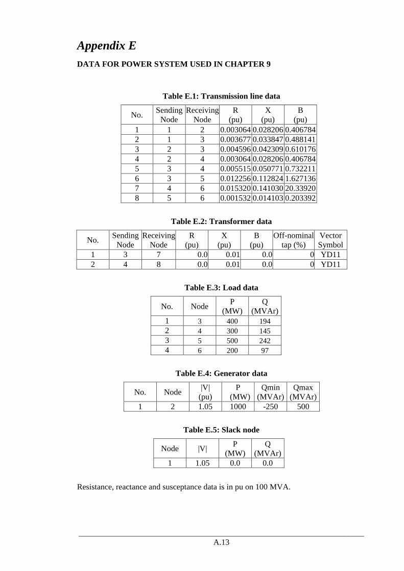
______________________________________________________________________A.13
Appendix E DATA FOR POWER SYSTEM USED IN CHAPTER 9
Table E.1: Transmission line data
No. Sending Node
Receiving Node
R (pu)
X (pu)
B (pu)
1 1 2 0.003064 0.028206 0.406784 2 1 3 0.003677 0.033847 0.488141 3 2 3 0.004596 0.042309 0.610176 4 2 4 0.003064 0.028206 0.406784 5 3 4 0.005515 0.050771 0.732211 6 3 5 0.012256 0.112824 1.627136 7 4 6 0.015320 0.141030 20.33920 8 5 6 0.001532 0.014103 0.203392
Table E.2: Transformer data
No. Sending Node
Receiving Node
R (pu)
X (pu)
B (pu)
Off-nominal tap (%)
Vector Symbol
1 3 7 0.0 0.01 0.0 0 YD11 2 4 8 0.0 0.01 0.0 0 YD11
Table E.3: Load data
No. Node P
(MW) Q
(MVAr) 1 3 400 194 2 4 300 145 3 5 500 242 4 6 200 97
Table E.4: Generator data
No. Node |V|
(pu) P
(MW) Qmin
(MVAr) Qmax
(MVAr) 1 2 1.05 1000 -250 500
Table E.5: Slack node
Node |V| P
(MW) Q
(MVAr) 1 1.05 0.0 0.0
Resistance, reactance and susceptance data is in pu on 100 MVA.

______________________________________________________________________A.14
Appendix F DATA FOR POWER SYSTEM USED IN CHAPTER 10
Table F.1: Transmission line data
No. Sending Node
Receiving Node
R (pu)
X (pu)
B (pu)
1 17 3 0.0044 0.0310 0.3731 2 17 4 0.0034 0.0310 0.3731 3 2 3 0.0089 0.0620 0.7461 4 2 5 0.0155 0.1085 1.3057 5 6 8 0.0086 0.0775 0.9326 6 6 10 0.0155 0.1085 1.3057 7 6 12 0.0069 0.0620 0.7461 8 7 11 0.0199 0.1395 1.6788 9 7 8 0.0066 0.0465 0.5596
Table F.2: LTC Transformer data
No. Sending Node
Receiving Node
R (pu)
X (pu)
B (pu)
|Vref| (pu)
Vector Symbol
1 1 4 0.0 0.01 0.0 1.03 YD11 2 2 5 0.0 0.01 0.0 1.02 YD11 3 3 6 0.0 0.01 0.0 1.03 YD11
Table F.3: Load data
No. Node P
(MW) Q
(MVAr) 1 6 200 90 2 7 400 130 3 8 800 390 4 9 600 290
Table F.4: Generator data
No. Node |V|
(pu) P
(MW) Qmin
(MVAr) Qmax
(MVAr) 1 2 1.0 700 -150 300 2 3 1.0 700 -150 300
Table F.5: Slack node
Node |V| P
(MW) Q
(MVAr) 1 1.00 0.0 0.0

______________________________________________________________________A.15
Table F.6: Data for impedance of shunt and series converter transformers of UPFC
Shunt Converter (pu) Series Converter (pu)
Resistance Reactance Resistance Reactance
0.0 0.01 0.0 0.01
Resistance, reactance and susceptance data is in pu on 100 MVA.

______________________________________________________________________A.16
Appendix G PUBLICATIONS
1. Nguyen, T.T., and Nguyen, V.L.: ‘Application of wide-area network of phasor
measurements for secondary voltage control in power systems with FACTS
controllers’, Proceedings of IEEE PES General Meeting, San Francisco, USA, June
2005, 3, pp. 2927-2934.
2. Nguyen, T.T., and Nguyen, V.L.: ‘Dynamical model of unified power flow
controllers in load-flow analysis’, Proceedings of IEEE PES General Meeting,
Montreal, Canada, June 2006.
3. Nguyen, T.T., and Nguyen, V.L.: ‘Representation of line optimisation control in
unified power flow controller model for power-flow analysis’, IET Generation,
Transmission and Distribution, 2007, 1, (5), pp. 714 – 723.
4. Nguyen, T.T., and Nguyen, V.L.: ‘Power system security restoration by secondary
control’, Proceedings of IEEE PES General Meeting, Florida, USA, June 2007.

______________________________________________________________________A.17
Appendix H CASE STUDIES PRESENTED IN THE THESIS
Case
Study Chapter Description Purpose
1 4
Application of the dynamic simulation-based UPFC model on steady-state analysis of a typical power system when discounting the UPFC operating limits.
Illustrate the solution trajectory during NR power-flow solution sequence.
2 4
Application of the dynamic simulation-based UPFC model on steady-state analysis of a typical power system taking into account the UPFC operating limits and relative priority in control functions.
Present the constraint resolution when the series converter voltage magnitude limit is active and the reference of lower priority (reactive-power flow) needs to be modified.
3 4
Application of the dynamic simulation-based UPFC model to maximise the active-power flow in a transmission line taking into account the UPFC operating limits and relative priority in control functions.
Present the constraint resolution when the series converter voltage magnitude limit is active and the references of lower priority (reactive-power flow and voltage magnitude references) need to be modified.
4 6
Application of the new UPFC model with LOC representation and the Newton optimisation algorithm augmented by the continuation method for the analysis and design of a long-distance transmission interconnection which depends on a UPFC for control and operation.
To justify the need of using a UPFC to solve a practical problem, and to illustrate the flexibility and generality of the proposed UPFC model in the constraint resolution taking into account the relative priorities in control functions.
5 8
Application of the secondary voltage control in a representative power system to control system voltage magnitudes subsequent to a contingency of a line outage. The controllers implemented comprise generator excitation controllers, SVC and STATCOM
To present the performance of the secondary voltage control and responses of a power system subsequent to the most severe line outage which leads to an unacceptable system voltage profile.

______________________________________________________________________A.18
Case
Study Chapter Description Purpose
6 9
Application of the secondary control for restoring power system security subsequent to a disturbance of a large load demand increase. Apart from generator excitations, the controllers implemented in the secondary control comprise both shunt compensators (SVC and STATCOM) and series compensators (TCSC).
To present the performance of the secondary control and responses of a power system subsequent to a significant load demand increase which leads to an unacceptable system voltage profile and an overload in a transmission line.
7 10
Application of the robust pilot-node based secondary control for power system security restoration subsequent to a disturbance of a load demand increase. Controllers consist of LTC transformers and UPFC.
To present the performance of the robust pilot-node based secondary control to restore the power system security subsequent to a significant increase in load demand at a node which leads to an unacceptable system voltage profile.
8 10
Application of robust pilot-node based secondary control for power system security restoration subsequent to a contingency of a transmission line outage. Controllers consist of LTC transformers and UPFC.
To present the performance of the robust pilot-node based secondary control to restore the power system security subsequent to a line outage which causes an unacceptable system voltage profile and overload in a transmission line.

1
Abstract-- Drawing on system voltages obtained from phasor
measurement units (PMUs) and wide-area communication network, a secondary voltage control formulation is developed, with particular reference to a power system having SVCs and STATCOMs. Based on the system load-flow equations linearised about the operating point defined by measured nodal voltages, the control procedure is formulated in terms of constrained optimisation with a quadratic objective function and a set of linear constraints derived from operating limits of reactive-power compensation systems and generators. The variables in the optimisation are the reference voltages of SVCs, STATCOMs and synchronous generators. The problem formulated is solved by standard quadratic programming method which is well-established and efficient in terms of computing time requirement in the context of online application. The procedure developed is applicable to any changes in loads and/or system configuration. Representative results of voltage control co-ordination are presented in the paper.
Index Terms-- FACTS, phasor measurement units application, secondary voltage control.
I. INTRODUCTION
ITH the widespread application of FACTS devices in power systems at present, secondary voltage
control [1]-[3] takes on a role of increasing importance. A recent paper [4] reported the development of a co-ordinated secondary voltage control procedure based on a fuzzy controller which co-ordinates the control of reference voltages of individual SVCs and STATCOMs. The procedure draws on local voltage measurements and estimation of voltages at adjacent nodes for secondary voltage control purpose. However, it has been indicated in [2] that if only some of the voltages are available in the measurements, then the performance of secondary voltage control can be degraded. With the present availability of phasor measurement units (PMUs) and extensive communication networks, the present paper proposes a new co-ordinated secondary voltage control scheme for power systems having SVCs and/or STATCOMs, based on synchronised voltage measurements for all nodes. The objective is to enhance the performance of the secondary
T. T. Nguyen and V. L. Nguyen are with the School of Electrical, Electronic and Computer Engineering at The University of Western Australia, Crawley, Western Australia 6009.
voltage control by using a wide-area network of phasor measurements. The application of wide-area network of phasor measurements in the context of protection and control, including emergency control, has recently been proposed in [5], [ 6]. The secondary voltage control procedure developed in the paper is based on the linearisation of the power system load-flow equations about the current operating point defined by nodal voltages obtained from PMUs. Using the voltages derived from PMUs, an objective function representing the error or difference between the actual operating voltage magnitudes and the required or target voltage magnitudes is formed. The secondary voltage control problem is transformed into a constrained optimisation in which the objective function is minimised with respect to the variables representing voltage reference input signals to SVCs, STATCOMs and synchronous generators. Following the linearisation of the load-flow equations, the objective function formed is a quadratic form in the variables used in the optimisation. The inequality constraints in the minimisation are linear ones which are associated with operating limits of SVCs, STATCOMs and synchronous generators. The formulation is, therefore, that of a standard quadratic programming problem for which efficient and fast solution method has been well-developed. This is a key feature of the formulation developed in the context of online application in relation to secondary voltage control. The control procedure is a general one which is applicable to any load variations and/or changes in power system configurations, including those arising from contingencies. Interactions amongst generators, SVCs and STATCOMs are fully taken into account. The co-ordinated control procedure is simulated in the MATLAB environment, and results for a representative power system are presented in the paper.
II. MODELS OF POWER SYSTEMS ELEMENTS
A. Principles
In the time scale relevant to secondary voltage control, the power systems model adopted is that in steady-state operating condition. Moreover, as the control period or cycle is
Application of Wide-Area Network of Phasor Measurements for Secondary Voltage Control in
Power Systems with FACTS Controllers T. T. Nguyen and V. L. Nguyen
W

2
relatively short, it is appropriate to assume that the load demand and active-power generation schedule together with system configuration do not change in the period [1]-[4 ].
Based on these principles, the following sections give in a summary form the models of individual items of plant which will be used later for developing the co-ordination strategy for secondary voltage control.
B. Load
With specified load active- and reactive-power demand, the load-flow equations for a load node k are given in:
ksk PP = (1)
ksk QQ = (2)
In (1) and (2), Pk and Qk are nodal active- and reactive-power, the expression of which are derived from the steady-state power system model referred to in section II.A. They are functions of system voltages and reference input voltage signals to generators and voltage controllers such as SVCs and STATCOMs. Pks and Qks are specified active- and reactive-power demand which are taken to be constant in a given control period.
C. Generator
With active-power generation specified, the load-flow equation in (1) is still applicable in the case of a generator node k:
ksk PP = (3) where Pks is active-power generation schedule of the generator at node k.
The second constraint represents the voltage magnitude control at the generator terminal when generator reactive-power is within operating limits:
refgenkk V || =V (4)
kgenkkgen QQQ max min ≤≤ (5)
In (4), |Vk| and Vrefgenk are voltage magnitude of the generator at node k and its reference value, respectively. In (5), Qgen min k and Qgen max k are reactive-power absorption and generation limits of the generator at node k, respectively.
When one of the inequalities in (5) is violated, generator reactive-power is set at the limit value, and the voltage magnitude control is released.
D. SVC and STATCOM
In Fig. 1 is shown a typical arrangement for connecting via a transformer a reactive-power compensator of either the SVC or STATCOM type [7].
The active- and reactive-power constraint equations in (1) and (2) are applicable to the high-voltage node which is a load node:
HksHk PP = (6)
HksHk QQ = (7)
where PHk and QHk are nodal active- and reactive-power at the high-voltage node. In (6) and (7), PHks and QHks are specified active- and reactive-power demand at the node. Fig. 1. Typical SVC and STATCOM arrangement.
However, there is another constraint at the high-voltage
node in Fig. 1 as its voltage magnitude is controlled in accordance with the V-I characteristic of Fig. 2 [7]:
Tkkrefkk IaV . || +=HV (8)
In (8), |VHk| is the magnitude of the voltage at the high-voltage node of SVC or STATCOM k; Vrefk, ak and ITk are reference voltage, slope reactance and current of SVC or STATCOM k, respectively.
Fig. 2. Voltage-current characteristic. ____ SVC ---- STATCOM
The linear control represented by (8) is valid only when the operating limits of SVC or STATCOM are not exceeded. For SVC, the operating limits are specified in terms of susceptances:
CsvcksvckLsvck BBB ≤≤ (9) where Bsvck, BCsvck and BLsvc are equivalent susceptance, limit of capacitive and inductive susceptance of SVC k, respectively.
For STATCOM, the operating limits are expressed in terms of currents: capacitive current limit ILsta and inductive
VHk
Compensator
VLk
Coupling Transformer
ITk
PHks
QHks
ITk
|VHk|
ILk ICk 0
Vrefk

3
current limit ICsta LstakstakCstak III ≤≤ (10)
When one of the inequality constraints in (9) is violated, the voltage control as defined in (8) is released, and the SVC model is represented as a constant shunt susceptance which takes the limiting value.
Similarly, when one of the inequalities in (10) is violated, the STATCOM model is that of a constant current source, the value of which is set to the limiting value whilst the voltage control function as given in (8) is no longer applicable.
For both SVC and STATCOM and when their active-power losses are discounted, the following active-power constraint at the low-voltage node applies:
0=LkP (11)
where PLk is active-power at the low-voltage node of SVC or STATCOM k.
E. Discussion
The equations derived from the steady-state models in sections II.B – II.D contain nonlinear terms in voltages. They are directly suitable for off-line analysis in which computing time is not a critical issue. However, the nonlinear equations do not give a direct and linear relationship between the system voltages and the reference input signals to the primary control loops of SVCs, STATCOMs and generators. Optimal control strategy based on nonlinear equations of the form given in (1) -(11) requires excessive computing time which is not appropriate for online application in secondary voltage control.
Given the constraint in terms of computing time, the following section develops linearised models which give explicit and linear relationships between system voltage magnitudes and controllers reference input signals. This allows the development of a secondary voltage control strategy based on optimisation in which the objective function is quadratic, and all of the inequality constraints are linear in control variables.
III. SENSITIVITY MATRIX OF POWER SYSTEM
A. Linearised System Model
Steady-state condition of a power system is described by nodal power equations given in:
)|,(| θfP VP = (12)
)|,(| θfQ VQ = (13)
where P and Q are vectors of nodal active- and reactive-power; |V| and θ are vectors of nodal voltage magnitudes and phase angles, and fP and fQ are nonlinear vector functions. Equations (12) and (13) do not include those for the slack node. By linearising (12) and (13) about (|V|, θ) received from PMUs, the nodal active- and reactive-power changes are expressed in terms of the voltage magnitude and the phase
angle deviations ∆|V|, ∆θ:
θθ
PV
VP
P ∆∂∂+∆
∂∂=∆ ||
|| (14)
θθ
QV
VQ
Q ∆∂∂+∆
∂∂=∆ ||
|| (15)
According to the assumptions in section II.A, active-power at all nodes, excepting the slack node, does not change. From (14), ∆θ is expressed in terms of ∆|V| in:
||||
1
VVP
θ
Pθ ∆
∂∂
⎥⎦
⎤⎢⎣
⎡
∂∂−=∆
−
(16)
Substituting ∆θ in (16) into (15) yields:
|| VAQ ∆=∆ (17)
where ||||
1
VP
θ
Pθ
QVQ
A∂
∂⎥⎦
⎤⎢⎣
⎡
∂∂
∂∂−
∂∂=
−
(18)
If there are n1 load nodes which have no SVC or STATCOM connections, n2 load nodes connected to the high- voltage side of SVCs or STATCOMs, and n3 generator nodes then the number of nodes excluding the slack node is n=n1+2n2+n3, including low-voltage nodes of SVCs and STATCOMs. Dimension of A is n x n. In order to develop the relation amongst the changes in system voltages, ∆Q, A and ∆V in (17) are first partitioned according to node types to give:
⎥⎥⎥⎥
⎦
⎤
⎢⎢⎢⎢
⎣
⎡
∆∆∆∆
⎥⎥⎥⎥
⎦
⎤
⎢⎢⎢⎢
⎣
⎡
=
⎥⎥⎥⎥
⎦
⎤
⎢⎢⎢⎢
⎣
⎡
∆∆∆∆
4
3
2
1
44434241
34333231
24232221
14131211
4
3
2
1
V
V
V
V
AAAA
AAAA
AAAA
AAAA
Q
Q
Q
Q
(19)
In (19), subscript 1 identifies load nodes without direct connections to SVCs or STATCOMs; subscript 2 load nodes with SVCs or STATCOMs connections; subscript 3 generator nodes, and subscript 4 low-voltage nodes of SVCs or STATCOMs. Similar to nodal active-power, the nodal reactive-powers at load nodes do not change. Using 01 =∆Q and 02 =∆Q in (19) gives:
0
V
V
V
V
AAAA
AAAA=
⎥⎥⎥⎥
⎦
⎤
⎢⎢⎢⎢
⎣
⎡
∆∆∆∆
⎥⎦
⎤⎢⎣
⎡
||
||
||
||
4
3
2
1
24232221
14131211 (20)
Equation (20) gives a relation amongst the changes in system voltage magnitudes when the assumption in II.A is valid. However, this relation needs to be combined with the voltage control characteristics of SVCs, STATCOMs and

4
generators for deriving the strategy for secondary voltage control. For this purpose, it is required first to form all of the equations for SVCs, STATCOMs and generators in a linear form.
B. Linear Models of Generators, SVCs and STATCOMs
1) Generator: From (4), the relationship between the change in voltage magnitude of a generator and its voltage reference is expressed as:
refgenkV∆=∆ || kV (21)
2) SVC and STATCOM: If the resistance of the coupling transformer is discounted, then (8) is given in terms of voltage magnitudes:
|)||(| || LkHkTk
krefcomkHk
x
aV VVV −+= (22)
where xTk is coupling transformer leakage reactance; Vrefcomk is the voltage reference value of SVC or STATCOM. The relationship between the changes in voltage magnitudes of nodes relating to SVC or STATCOM and the change in its voltage reference is given in, following the rearrangement of (22) and applying the differential operator:
refcomkLkTk
kHk
Tk
kV
x
a
x
a ∆=∆+∆− ||||)1( VV (23)
or
refcomkLk
Hk
Tk
k
Tk
kV
x
a
x
a ∆=⎥⎦
⎤⎢⎣
⎡
∆∆
⎥⎦
⎤⎢⎣
⎡ − ||
|| )1(
VV
(24)
Equations (21) and (24) are for individual generators and SVCs or STATCOMs. Assembling these individual equations into vector/matrix form leads to:
ref
4
3
2
V
V
V
V
B ∆=⎥⎥⎥
⎦
⎤
⎢⎢⎢
⎣
⎡
∆∆∆
||
||
||
(25)
where ⎥⎦
⎤⎢⎣
⎡
∆∆
=∆refgen
refcomref
V
VV (26)
Elements of matrix B are coefficients in (21) and (24). In (26), ∆Vrefcom is a vector the elements of which are individual changes in voltage references in SVCs and STATCOMs; ∆Vrefgen is the vector of voltage reference changes in generators. Equation (25) establishes the relation between the changes in terminal voltage magnitudes at generators, SVCs and STATCOMs and their reference signals changes. The equation will be combined with (20) to give the secondary voltage control law.
C. System Sensitivity Matrix
For the purpose of including ∆|V1| in (25) so that the vectors of system voltage changes in (20) and (25) have the same dimension and elements, (25) is augmented as:
[ ] ref
1
V
V
V
V
V
B0 ∆=
⎥⎥⎥⎥
⎦
⎤
⎢⎢⎢⎢
⎣
⎡
∆∆∆∆
||
||
||
||
4
3
2 1 M (27)
where 01 is a zero matrix of dimension (n2+n3) x (n1). Solving matrix equations (20) and (27) gives:
||
||
||
||
4
3
2
1
⎥⎦
⎤⎢⎣
⎡
∆=
⎥⎥⎥⎥
⎦
⎤
⎢⎢⎢⎢
⎣
⎡
∆∆∆∆
refV
0C
V
V
V
V
(28)
where
1
1
24232221
14131211−
⎥⎥⎥
⎦
⎤
⎢⎢⎢
⎣
⎡
=B0
AAAA
AAAA
C (29)
In (28), 0 is a zero vector of (n1+n2) elements. As the elements in the first (n1+n2) rows of the vector on
the RHS of (28) are zero, the first (n1+n2) columns of matrix C do not make any contribution in the solution for the vector of system voltage magnitude changes on the LHS of (28). The following partitioning of matrix C allows the solution vector of nodal voltage magnitudes changes to be formed directly in
terms of ∆Vref:
[ ]
3221
21 CCC M
nnnnn
++= (30)
Substituting C in (30) into (28) gives:
||
||
||
||
.2
4
3
2
1
refVC
V
V
V
V
∆=
⎥⎥⎥⎥
⎦
⎤
⎢⎢⎢⎢
⎣
⎡
∆∆∆∆
(31)
For applying voltage control on all of the load nodes, matrix C2 in (31) is partitioned into submatrices a and b to give separate equations related to load nodes, and the remaining nodes comprising those on the low-voltage sides of SVCs and STATCOMs, and generator nodes:
⎥⎥⎥
⎦
⎤
⎢⎢⎢
⎣
⎡
=b
a
C2 L (32)
Two separate equation sets are then formed, using (32) in (31):
refVaV
V∆=⎥
⎦
⎤⎢⎣
⎡
∆∆
. ||
||
2
1 (33)
and refVbV
V∆=⎥
⎦
⎤⎢⎣
⎡
∆∆
.||
||
4
3 (34)

5
D. Discussion
Equation set (33) will be used later to form an objective function in the optimization in which load nodes voltage deviations from target profile are to be minimized. Equation set (34) in conjunction with specified voltage limits at generator nodes and nodes on the low-voltage side of SVCs and STATCOMs will form a secondary objective expressed as inequality constraint in the overall optimization adopted for secondary voltage control. However, there are additional inequality constraints to be considered. They relate to generator reactive-power limits, SVCs susceptance limits and STATCOMs operating current limits. The next section will derive the sensitivity of generator reactive-powers, SVCs susceptances and STATCOMs currents with respect to the changes in voltage reference signals.
E. Controller Sensitivity Matrices
1) Generator Reactive-Power: From (19), the change in reactive-power of generators is:
[ ]⎥⎥⎥⎥
⎦
⎤
⎢⎢⎢⎢
⎣
⎡
∆∆∆∆
=∆
||
||
||
||
3
4
3
2
1
34333231
V
V
V
V
AAAAQ (35)
Substituting (31) into (35) gives: ref3 VcQ ∆=∆ . (36)
where [ ] 2 . CAAAAc 34333231= (37)
2) SVC Susceptance: On discounting the resistance of the coupling
transformer, the equivalent susceptance of SVC k is formed in:
||
||||
HkTk
LkHksvck
xB
VVV −−= (38)
Linearising (38) yields
||)||
1(||)
||
||(
2Lk
TkHkHk
TkHk
Lksvck
xxB V
VV
VV ∆+∆−=∆
(39) Equation (39) applies to one SVC. Extending to a
number of SVCs leads to the following relation in matrix/vector form:
⎥⎥⎥⎥
⎦
⎤
⎢⎢⎢⎢
⎣
⎡
∆∆∆∆
=∆
||
||
||
||
2
1
4
3svc
V
V
V
V
DΒ (40)
Matrix D in (40) is assembled from the coefficients on the RHS of (39) for individual SVCs. ∆Bsvc is the vector of changes in susceptances of individual SVCs. As ∆Bsvc depends directly only on the changes in the voltages on the high- and low-voltage nodes of SVCs, columns of D in the positions which correspond to the changes in voltages at other
nodes in the system are set to zero. Using (31) in (40) gives:
refsvc VdB ∆=∆ . (41) In (41):
2CDd . = (42) 3) STATCOM Current:
If the resistance in the STATCOM coupling transformer is neglected, then STATCOM operating current is expressed in:
Tk
LkHkstak
xI
|||| VV −= (43)
From (43), the change in STATCOM current is formed in terms of changes in voltages:
||1
||1
LkTk
HkTk
stakxx
I VV ∆−∆=∆ (44)
Extending (44) to a number of STATCOMs leads to the following equation in matrix/vector form:
⎥⎥⎥⎥
⎦
⎤
⎢⎢⎢⎢
⎣
⎡
∆∆∆∆
=∆
||
||
||
||
2
1
4
3sta
V
V
V
V
EI (45)
In (45), ∆Ista is the vector of operating current changes in individual STATCOMs; E is formed from the coefficients on the RHS of (44), and similar to SVCs, columns of E which do not correspond to the high- and low-voltage nodes of STATCOMs are set to zero.
Substituting (31) into (45) gives:
refsta VeI ∆=∆ . (46) In (46):
2CEe . = (47)
IV. CONTROL STRATEGY
The objective of the secondary voltage control is to determine the optimal set of controllers voltage references to minimize the difference between the magnitudes of voltages at the load nodes in the system and their specified or target voltage values.
If VL0 is a vector of the current load node voltage values
in phasor form received from PMUs, then the difference between | VL
0| and specified target values in vector Vtarget is: || 0
LtargetE VVf −= (48)
When the magnitude of vector fE is less than a pre-set tolerance, no control action in relation to adjusting controllers reference voltage settings is required until the next secondary voltage control cycle. Otherwise, the reference settings will be modified to achieve the objective of secondary voltage control.
From (33), changes in controllers reference settings lead to load node voltage magnitude changes from the current values given by:

6
refL VaV ∆=∆ . || (49)
The purpose is to determine ∆Vref so that the difference between fE in (48) and ∆|VL| in (49) is minimized.
An objective function having a quadratic form in ∆Vref is defined:
[ ] [ ]ELEL fVfV −∆−∆= |||| TF (50)
or, from (49):
[ ] [ ]ErefEref fVafVa −∆−∆= .. TF (51)
If required, a weighting vector is included in forming the objective function F to give priority to voltage control of selected nodes.
The objective function F in (51) is minimized with respect to ∆Vref subject to inequality constraints related to limits on voltage magnitudes of generator nodes and low-voltage nodes of SVCs and STATCOMs, generator reactive-powers, SVCs susceptances and STATCOMs operating currents. The set of inequality constraints are given in the following, drawing on the system sensitivity matrix formed in section III.C and sensitivity matrices derived in section III.E:
maxmin . VVbV ref ∆≤∆≤∆ (52) maxmin . QVcQ ref ∆≤∆≤∆ (53)
maxmin . BVdB ref ∆≤∆≤∆ (54) maxmin . ΙVeI ref ∆≤∆≤∆ (55)
In (52), ∆Vmin and ∆Vmax are vectors of deviations between the current operating voltage magnitudes of generator nodes, low-voltage nodes of SVCs and STATCOMs and the allowable minimum and maximum voltage magnitudes at these nodes respectively.
In (53), ∆Qmin and ∆Qmax are vectors of the differences between the current operating reactive-powers of generators and their minimum and maximum reactive-power limits.
In (54), ∆Bmin and ∆Bmax are vectors of the differences between the current operating equivalent susceptances of SVCs and their inductive limits and capacitive limits respectively.
In (55), ∆Imin and ∆Imax are vectors of the differences between the current operating currents of STATCOMs and their minimum and maximum limits respectively.
In the above, the secondary voltage control strategy is expressed as a constrained optimization, in which the objective function is a quadratic form in the control variables, and the inequality constraints are linear. Efficient and robust method such as that based on quasi-Newton algorithm is available for solving this standard quadratic programming problem.
The dimension of the vector of control variables in the optimization is relatively low in comparison with the number of power network nodes. Similarly, the number of inequality constraints in (52) – (55) is also low.
The optimal solution for ∆Vref provided by the optimization augments the current vector of controllers reference settings, ∆Vref
0, to give:
refrefref VVV ∆+= 0 (56) In (56), Vref is the vector of optimal reference settings for
the controllers.
V. SECONDARY VOLTAGE CONTROL LOOP
In Fig. 3 is shown in block diagram form the secondary voltage control loop which implements the control strategy developed in section IV.
The block “control co-ordination” performs all of the required calculation including determining the coefficient matrices for use in the constrained optimization. It receives the relevant data from PMUs via the wide-area network, and power system database. The required power system configuration is determined from telemetered data related to circuit-breakers and isolators statuses [8]. The output from
the control co-ordination is vector Vref the elements of which are input to the relevant generators, SVCs and STATCOMs which participate in the secondary voltage control.
Fig. 3. Scheme of the secondary voltage control. One practical option is to include the control loop in Fig. 3
in the Energy Management System (EMS) which will provide supporting functions required in the control co-ordination.
VI. SIMULATION RESULTS
This section presents the simulation results carried out using a representative power system shown in Fig. 4
The power system consists of 24 nodes including the slack node 1. There are 5 generators, 1 SVC and 1 STATCOM used to control the voltage profile of load nodes.
The limits of reactive-power of generators are given in Table I.
The lower and upper limits for SVC susceptance are –1.00 pu and 1.00 pu on 100 MVA respectively. The lower and upper limits for STATCOM current are –0.50 pu and 0.50 pu on 100 MVA respectively. The slope reactances of both the SVC and STATCOM are set to 2% on 100 MVA.
By standard load-flow analysis, the current operating point
Vref
CONTROL CO-ORDINATION
PMUs
POWER SYSTEM DATABASE
CIRCUIT-BREAKERS and ISOLATORS
STATUSES
POWER SYSTEM
POWER SYSTEM CONFIGURATION DETERMINATION

7
of the power system for a given load demand and generation schedule is obtained. For the purpose of quantifying the effects of generator reactive-power, SVC susceptance and STATCOM current limits, two cases are considered: the first is that when the limits are not represented; the second is that when limits are taken into account.
Fig. 4. Configuration of 24-node power system. TABLE I
LIMIT OF GENERATOR REACTVE-POWER
Generator Qmin
(pu on 100 MVA) Qmax
(pu on 100 MVA) 1 (at node 18) -1. 0 1.90 2 (at node 19) -0.60 1.20 3 (at node 20) -0.40 0.80 4 (at node 21) -0.60 1.20 5 (at node 22) -1. 0 1.80
In Fig. 5 is shown the system voltage profile for the current
operation in case 1 which indicates that voltages at some nodes are quite low.
With secondary voltage control applied in this case, and
using the control strategy developed in section IV with target voltages of 1.0 pu for all load nodes, the new system voltage profile is shown in Fig. 5. The comparison between the current voltage profile and the new one in Fig. 5 confirms the significant improvement following the control based on the new reference voltage settings.
Fig. 5. Voltage profiles of the power system in case 1.
---- Current operating condition ___ New operating condition obtained from optimization -.-. New operating condition determined by load-flow
In Table II, the new voltage reference setting are given and
compared with the current settings. TABLE II
VOLTAGE REFERENCE SETTINGS IN CASE 1
Controller Current settings New settings Generator 1 1.000 1.026 Generator 2 1.000 1.050 Generator 3 1.000 1.050 Generator 4 1.000 1.050 Generator 5 1.000 1.030
SVC 1.000 1.019 STATCOM 1.000 1.027 The current operating point in case 2 is different from case
1, due to limits being applied on generators, SVC and STATCOM. The voltage profile in current operation for case 2 is given in Fig. 6. Some nodes in the system have very low voltage magnitudes. It is proposed to apply secondary voltage control, with appropriate limits for all of the controllers, in this case.
Following the control achieved with new reference voltage settings given in Table III, the voltage profile improves as shown in Fig. 6. However, the improvement is not as great as that in case 1 due to operating limits being imposed on the controllers.
In both cases 1 and 2, full load-flow analyses are carried out with the new reference settings to verify that the linearised model adopted for secondary voltage control is a valid one. In the comparisons in Figs. 5 and 6, the full load-flow solutions
STATCOM
24
132 kV
18 22
17
1
16
4 5
6 7
8
22 9
19 10 11
12 13
14 15
20 21
3
SVC
23
330 kV
2

8
are almost identical to those from the linearised model.
Fig. 6. Voltage profiles of the power system in case 2.
---- Current operating condition ___ New operating condition obtained from optimization -.-. New operating condition determined by load-flow
TABLE III VOLTAGE REFERENCE SETTINGS IN CASE 2
Controller Current settings New settings Generator 1 1.000 1.009 Generator 2 1.000 1.050 Generator 3 1.000 1.042 Generator 4 1.000 1.050 Generator 5 1.000 1.007
SVC 1.000 1.031 STATCOM 1.000 1.036
VII. CONCLUSION
The paper has successfully developed a control co-ordination strategy based on constrained optimization applicable to secondary voltage control in power systems which have FACTS controllers. Central to the strategy is the application of information available from a wide-area network of phasor measurements. The information on voltage phasors allows a linear system model to be formed and used in developing the control strategy. The formulation in terms of quadratic programming problem having relatively low number of control variables and linear inequality constraints lends itself to efficient and fast solution, as required in secondary voltage control.
The algorithm in the control strategy has been validated with simulation studies using a representative power network. Full load-flow solutions have been used to confirm the correctness of the proposed control co-ordination method. The possibility of practical implementation of the method within the EMS is referred to and discussed in the paper.
VIII. ACKNOWLEDGMENT
The authors gratefully acknowledge the support of the Energy Systems Centre at The University of Western
Australia for the research work reported in the paper. They express their appreciation to The University of Western Australia for permission to publish the paper
IX. REFERENCES [1] J.P. Paul, J.Y. Leost, and J.M. Tesseron, “Survey of the secondary voltage
control in France: present realization and investigations,” IEEE Trans. Power Systems, vol. 2, no. 2, pp. 505-511, May 1987.
[2] A. Stankovie, M. Elic, and D. Maratukulam, “Recent results in secondary voltage control of power systems,” IEEE/PES 1990 Winter Meeting, Atlanta, Georgia, , pp.94-101, 1990.
[3] B. Marinescu, and H. Bourles, “Robust predictive control for the flexible coordinated secondary voltage control of large-scale power systems,” IEEE Trans. Power Systems, vol. 14, no. 4, pp. 1262-1268, 1999.
[4] H. F. Wang, H. Li, and H. Chen, “Coordinated secondary voltage control to eliminate voltage violations in power system contingencies,” IEEE Trans. Power Systems, vol. 18, no. 2, pp. 588-595, May 2003.
[5] B. Milosevic, and M. Begovic, “Voltage-stability protection and control using a wide-area network of phasor measurements,” IEEE Trans. Power S ystems, vol. 18, no. 1, pp. 121-127, 2003.
[6] Working Group C-6, System Protection Subcommittee, IEEE PES Power System Relaying Committee, “Wide area protection and emergency control”. (Final Report)
[7] CIGRE TF 38.01.08: “Modeling of power electronics equipment (FACTS) in load flow and stability programs: a representation guide for power system planning and analysis”, 1998
[8] W. D. Humpage, K. P. Wong, and T. T. Nguyen, ”PROLOG network-graph generation in system surveillance,” Electric Power System Research, no.9, pp. 37-48, 1985.
X. BIOGRAPHIES
T.T. Nguyen was born in Saigon, Vietnam, in 1956. Currently, he is an Associate Professor at The University of Western Australia. He was an invited lecturer in power system short courses in Thailand and Indonesia (1985), the Philippines (1986), Malaysia (1986, 1990), Singapore (1992), Vietnam (1999, 2000, 2003) and in the inaugural course (1991) in the national series of short course in power systems sponsored by the Electricity Supply Association of Australia
(ESAA). He was the Director of the ESAA 2000 Residential School in Electric Power Engineering. His interests include power systems modeling, analysis and design; power systems control and protection, quality of supply, transmission asset management and applications of neural networks and wavelet networks in power systems. He has published more than 100 papers in international literature, three undergraduate textbooks, and four short course textbooks. Professor Nguyen was awarded the Sir John Madsen Medal of the Institution of Engineers, Australia in 1981 and 1990. He serves on CIGRE International Task Forces. He was the Chairman of the Australasian Universities Power Engineering Conference in 1995.
V.L. Nguyen was born in Ho Chi Minh City , Vietnam, on June 25, 1964. He received his BE in Electrical Engineering from Ho Chi Minh City University of Technology in 1986. Since then, he was appointed as an Associate Lecturer and then promoted to Lecturer in the same University. He is currently a PhD student under the supervision of Associate Professor T.T. Nguyen at the Energy Systems Centre, The University of Western Australia. His research interests are in the fields of power systems modeling, analysis and control with particular
reference to stability and FACTS.

1
Abstract-- Based on the novel concept of interpreting the
updated voltage solutions at each iteration in the Newton-Raphson (NR) load-flow analysis as dynamic variables, the paper develops a procedure for representing the unified power flow controllers (UPFCs) in the steady-state evaluation. Both the shunt converter and series converter control systems of a UPFC are modeled in their dynamical form with NR iterative step as the discrete independent variable in the load-flow analysis. The key advantage of the method developed is that of facilitating the process of constraint resolution during the NR solution sequence. Any priority in control functions pre-set in the UPFC controllers is automatically represented in the load-flow formulation. The method developed together with its software implementation is tested using a representative power network with UPFC.
Index Terms-- Dynamical model, Newton-Raphson load-flow, UPFC constraint resolution.
I. INTRODUCTION ECENT development of FACTS devices, including UPFCs, provides many benefits to power network control
which include maximization of the utilization of the transmission systems, real-time control of the power flow in a specified transmission circuit or path, and control-based expansion of the transmission system subject to stability and/or environmental constraints. These benefits are of particular importance at present in the context of the restructuring in the power supply industry and open transmission access. However, effective applications of FACTS devices require analysis facilities which include their models. The present paper has a focus on the development of UPFC model for steady-state load-flow analysis. The main difficulty encountered or reported in previously-published work on UPFC steady-state model is that of developing a systematic procedure for UPFCs constraint resolution during the load-flow iterative solution sequence. The difficulty arises from multiple limits that have to be complied with in UPFCs operation, and the need to take into account the relative priorities assigned to individual UPFC control functions when constraint resolution is required.
The previously-published UPFC models for steady-state analysis [1]-[4] are based on voltage-current relationships at the UPFC locations that are derived from the assumption that
T. T. Nguyen (email: [email protected]) and V. L. Nguyen (email: [email protected]) are with the School of Electrical, Electronic and Computer Engineering at The University of Western Australia, Crawley, Western Australia 6009.
all of the specified UPFC control objectives have been achieved. The equation describing the relationships are solved simultaneously with the power-flow equations of the system, using iterative solution technique such as that based on the Newton-Raphson (NR) algorithm. A separate set of inequality constraints for representing UPFCs operating limits is formed. In [5], a set of rules was used for handling the inequality constraints when one or more UPFC operating limits are violated during the iterative solution sequence. However, no substantiated basis was given in [5] for establishing the rules.
Further complication arises due to multiple control functions provided by a UPFC, and there is relative priority assigned to them. In the UPFC models reported in [2]-[4], [6] and [7], the relative control priority is not represented when one or more UPFC inequality constraints become active.
The objective of the present paper is to develop a new UPFC model for load-flow analysis, based on the explicit dynamic simulation of both the shunt converter and series converter controllers. The dynamic simulation is carried out in conjunction with the NR load-flow solution sequence. The updated voltages at each NR iterative step are interpreted as dynamic variables. The relevant variables are input to the UPFC controllers. The responses of controllers to the inputs, subject to the limits and priority specified in the controllers, are the voltage sources associated with the shunt and series converters. The voltage sources are input to power network at the UPFC locations for the subsequent NR iteration. The constraint resolution problem encountered in previous UPFC steady-state models in which there are interactions amongst the UPFC equations representing the control objectives and inequality constraints representing the operating limits is avoided completely. The relative priority in UPFC control is inherently taken into account in the new formulation via the direct simulation in a dynamical form of the UPFC controllers. The overall simulation can be considered to be a hybrid one in which dynamical model of the UPFC is combined with the NR load-flow model for power network.
The applications of the simulation technique are those in power systems planning and design where UPFCs are proposed. With the general simulation technique developed in the paper, the use of TNA [8] for system study will be avoided. The hybrid model together with its software implementation is validated using results obtained from the load-flow study of a representative test system.
Dynamical Model of Unified Power Flow Controllers in Load-flow Analysis
T. T. Nguyen and V. L. Nguyen
R
1-4244-0493-2/06/$20.00 ©2006 IEEE.

2
II. UPFC DYNAMICAL MODEL The properties and characteristics of a UPFC have
previously been studied and published in [1]-[6]. The basic scheme of the UPFC is shown in Fig. 1. It consists of two voltage source converters (VSCs): one is a shunt-connected VSC, and the other a series-connected VSC. The two VSCs are connected via a DC link, which includes a DC shunt capacitor.
Fig. 1. The UPFC Schematic Diagram.
The shunt converter controller is shown in Fig. 2 in a block diagram form [8]. The output from the shunt converter can be interpreted as a voltage source applied to the power system at node K, the magnitude and phase angle of which are adjusted by the controller to control the voltage magnitude at node K to a specified value, Vref, and keep the dc voltage constant. In Fig. 2, t is the independent time variable. In the digital implementation of the controller, the time variable takes a discrete form.
Fig. 2. Block Diagram of Shunt Converter Controller.
VK(t) and Vref: Voltage phasor of node K at t and its magnitude reference IE(t): Shunt converter current phasor at t Vdc(t) and Vdcref: DC voltage at t and its reference IEp(t) and IEq(t): In-phase and quadrature components of the shunt converter
current at t wrt the reference given by VK(t) IEpref(t) and IEqref(t): In-phase and quadrature components of required shunt
converter current at t VEp(t) and VEq(t): In-phase and quadrature components of the shunt converter
voltage source at t VE(t) and θE(t): Magnitude and angle of the shunt converter voltage source at t θK(t): Phase angle of voltage phasor VK(t)
Similarly, the series converter controller in a block diagram
form is given in Fig. 3. The functions of the controller are to control active- and reactive-power flows in the transmission line that has the UPFC. To achieve this control objective, the series controller adjusts both the magnitude and phase of the series voltage which is inserted into the transmission line.
Fig. 3. Block Diagram of Series Converter Controller. VL(t): Voltage phasor of node L at t VK(t): Voltage phasor of node K at t IB(t): Series converter current phasor at t Vdc(t): DC voltage at t Pref and Qref: Active- and reactive-power references VBp(t) and VBq(t): In-phase and quadrature component of the series voltage
at t VB(t) and θB(t): Magnitude and angle of the series voltage at t θK(t): Phase angle of voltage phasor VK(t) The output signals from the controllers in Figs. 2 and 3 are
input to the PWM (pulse-width-modulation) control system of the converters to achieve the required 3-phase voltage sources.
The operation of both the shunt converter and series converter are subject to limits which include:
- Maximum series voltage magnitude - Maximum series converter current - Maximum shunt converter current - Maximum line-side voltage of the UPFC - Minimum line-side voltage of the UPFC - Maximum active-power exchange between the series and
shunt converters These limits are represented in the controllers in forming
the outputs in real time. Separately, the UPFC has a second level of control by
which the reference inputs to the controllers are modified [8], when required, to achieve a pre-specified relative priority in control functions. In general, modifications of reference inputs are needed when one or more operating limits are violated.
For load-flow analysis, the UPFC can be represented in terms of two voltage sources, VE and VB, based on the outputs of the controllers, by the model of Fig. 4. ZE and ZB in Fig. 4 are the leakage impedances of the shunt and series converter transformers respectively.
θB(t)
Error Amplifier
VL(t)
SeriesInjectedVoltageLimiter
VBq(t)
Magnitudeand Angle Calculator
VBp(t)VB(t)
Σ
θK(t)
Limit Calculator
VL(t) VK(t)
IB(t) Vdc(t)
VK(t)
Σ
Pref
IBp(t)
Qref
Active/Reactive Current
Components Calculator
IBpref(t)
Σ
IBq(t)
Active/Reactive Current
Components Calculator
IBqref(t)
IB(t)
+_
+
_
+
+
Phase Locked Loop
transmission lineK L
DC link
shunt converter
series converter
. . . .
Vref
Vdcref
Vdc(t) θE(t)
Voltage Magnitude Calculator
Σ Error Amplifier
Shunt Reactive Current Limiter
Σ Error Amplifier
Σ
Σ Error Amplifier
Active/Reactive Current
Components Calculator
Limit Calculator
IE(t)
VK(t)
IEq(t)
IEp(t)
IEqref(t)
IEpref(t)
VEq(t) Magnitude and Angle Calculator
VEp(t) VE(t)
_
+
+
+
+ _
_
_ Σ
θK(t)
+
+Phase Locked Loop
VK(t)

3
Fig. 4. UPFC dynamical model.
III. UPFC DYNAMICAL REPRESENTATION IN LOAD-FLOW ANALYSIS
A. Principle In NR load-flow solution sequence, the voltage vector x at
iterative step p+1 is formed from that at step p using: ( )[ ] ( ))(. )()()1( 1 pppp xfxJxx −−=+ (1)
In (1), J is Jacobian matrix; f is a vector of residual functions.
Equation (1) can be interpreted as that of a discrete dynamical system in which the NR iterative step p is the discrete independent variable. Iterative step p then takes the role of the time variable in the controllers in Figs. 2 and 3. On this basis, it is proposed in the present work to use the solution for the power network at NR iterative step p in terms of nodal voltages and branch currents at the UPFC location as the inputs to the controllers in Figs. 2 and 3. The responses of the controllers to the inputs are then the voltage sources which are to be inserted into the power network model for the next NR solution step p+1.
In forming the responses which are the voltage sources used in the model of Fig. 4, the UPFC controllers operations, including the operating limits and control priority, are simulated dynamically. The differential equations which describe the controller dynamics are transformed into the difference equations (algebraic) in which NR iterative step is the independent variable. The dynamic simulation technique developed provides automatically constraint resolution when one or more operating limits are exceeded during the NR solution sequence whilst relative control priority is observed.
B. Implementation for Load-flow Analysis The controllers in Figs. 2 and 3 are interpreted for load-
flow analysis in terms of dynamical systems in Figs. 5 and 6 where the time variable is represented as NR iterative steps.
For the series converter, the output of the controller, on receiving the inputs derived from the NR solution at step p, is the series voltage VB (p+1) which is used directly in forming the load-flow equations at step p+1.
For the shunt converter, the preference in load-flow analysis is not to represent the dc side of the UPFC explicitly. The loop for dc voltage control is represented equivalently by active-power balance equation between the shunt and series converters from which the required value of the active component of the shunt current is derived. The voltage control
loop which is retained explicitly in the load-flow analysis gives the required reactive component of the shunt converter current.
Fig. 5. Block diagram for the series converter in load-flow environment.
Fig. 6. Block diagram for the shunt converter in load-flow environment. Further simplification is possible where the required shunt
converter current defined from its active and reactive components is used as a current injected into node K in the model of Fig. 4. With the use of shunt converter current injection, the shunt converter controller in Fig. 2 is simplified to that shown in Fig. 6. For NR iterative step (p+1), the current injection into node K, which is obtained from the controller of Fig. 6, is denoted by IE(p+1). In this way, the current control loops in Fig. 2 are not required in the load-flow analysis. On this basis, the model in Fig.4 is reduced to that of Fig. 7.
Fig. 7. UPFC dynamical model for load-flow analysis.
transmission lineVB(t)ZB K L
ZE
VE(t)
VB(p+1) ZB
IE(p+1)
K L transmission line
IEq(p+1)
IEp(p+1)
Magnitudeand Phase
Angle Calculator
IE(p+1)
ψE(p+1)
Vref
VK(p)
PB(p)
VK(p)
∆VK(p) Σ
_ + Error
Amplifier
Reactive Current Limiter
Active Current Limiter Σ
θK(p)
+
+
Active Current
Calculator
VB(p+1)
θB(p+1)
IBq(p)
IBp(p)
VBq(p+1)
VBp(p+1)
Pref Qref
VL(p) Current ReferenceCaculator
Error
Amplifier
∆IBq(p)
∆IBq(p)
Σ+
Σ_
+
_
VK(p)Series
Converter Current
Calculator
IBqref(p)
IBpref(p)
VL(p)
VB(p)
θK(p)
Limit
Calculator
VK(p)
VL(p)
IB(p)
Magnitudeand Phase
Angle Calculator
Σ+
+Series Injected Voltage Limiter

4
The load-flow equations for nodes K and L in Fig. 7 are now formed for the NR iterative step p+1, using the known series voltage source VB(p+1) and injected current IE(p+1) of the shunt converter.
The net nodal power at node K in Fig. 7 is given in, taking into account the shunt converter injected current IE(p+1) and series voltage VB(p+1):
( )[ ] ( )*
11.⎪⎭
⎪⎬⎫
⎪⎩
⎪⎨⎧
+−++−+
=+
∑ pp
jQP
EBLKBi
iKiK
KK
IVVVYVYV (2)
In (2), YKi is the element (K,i) of the admittance matrix of the power system, and YB=1/ZB .
If PKs, QKs are specified active- and reactive-power demand at node K, then the residual functions at node K are:
0=− KsK PP (3) 0=− KsK QQ (4)
Similarly, the net nodal power at node L in Fig. 7 is formed
by, including the contribution from the voltage source VB(p+1):
( )[ ]*
1.⎪⎭
⎪⎬⎫
⎪⎩
⎪⎨⎧
++−−=+ ∑ pjQP BLKBi
iLiLLL VVVYVYV (5)
In (5), YLi is the element (L,i) of the admittance matrix of the power system.
When there is no load demand at node L, the residual functions at that node are:
0=LP (6) 0=LQ (7)
Solving, by NR method, the four equations in (3), (4), (6) and (7) in conjunction with other standard load-flow equations gives nodal voltage solutions at step p+1.
The principal steps in simulation of UPFC in a dynamical form in load-flow analysis has been developed in this section. In the following, the detailed process of forming the series voltage source VB(p+1) and shunt converter injected current IE(p+1) will be derived, based on the controllers transfer function simulation.
IV. SERIES VOLTAGE SOURCE
A. Definitions To facilitate the subsequent development, relevant symbols
and variables are defined in this section. VK is used as the voltage reference phasor. Subscripts p and
q identify the in-phase and quadrature components of voltage/current with respect to the reference phasor. On this basis, the series voltage VB, line side voltage VL and series converter current IB have the following general form:
KjBqBpB ejVV θ)( +=V (8)
KjLqLpL ejVV θ)( +=V (9)
KjBqBpB ejII θ)( +=I (10)
In (8)-(10), θK is the phase angle of VK.
B. Transfer Function Simulation In the controller in Fig. 5, the active- and reactive-power
control specified in Pref and Qref respectively is converted to one of current control, using known line side voltage VL at step p.
The reference current for series converter is determined by, using Pref and Qref:
)()()()(
pjVpVjQP
pjIpILqLp
refrefBqrefBpref −
−=+ (11)
The reference current as calculated in (11) is then compared with the measured current, which is derived from load-flow voltage solution at step p as follows:
B
LqBqBp X
pVpVpI
)()()(
−= (12)
B
KLpBpBq X
pVpVpVpI
)()()( )(
−+−= (13)
In (12) and (13), XB is the series converter transformer reactance, and for simplicity, the resistance is discounted.
The error or the difference between the reference current value and the measured current is used in the current control loop to form the p and q components of the series voltage as follows, for integral control:
)]()(.[)()1( 1 pIpIKpVpV BqBqrefBpBp −+=+ (14)
)]()(.[)()1( 2 pIpIKpVpV BpBprefBqBq −+=+ (15)
In (14) and (15) K1 and K2 are derived from the controller gains. Although integral control has been assumed in (14) and (15), any other forms of controller can be simulated without difficulty. The controller outputs given in (14) and (15) are then subject to UPFC operating limits. The limit calculator in Fig. 5 determines the appropriate series voltage magnitude, based on the present information on UPFC voltages and currents. The set of inequalities to be satisfied in relation to series voltage magnitude, line side voltage magnitude, active-power exchange between series and shunt converters, and series current magnitude are given in:
max22
BBqBp VVV ≤+ (16)
min22 ).().( LBpBBqBqBKBp VIXVIXVV ≥−+++ (17)
max22 ).().( LBpBBqBqBKBp VIXVIXVV ≤−+++ (18)
max.. BBqBqBpBp PIVIV ≤+ (19)
max
22
BB
LqBq
B
LpKBp IX
VVX
VVV≤⎟⎟
⎠
⎞⎜⎜⎝
⎛ −+⎟⎟
⎠
⎞⎜⎜⎝
⎛ −+ (20)
The above inequalities apply to the series voltage for the next NR step p+1.

5
In (16), VBmax is the maximum allowable series voltage magnitude.
In (17) and (18), VLmin and VLmax are the minimum and the maximum allowable line side voltage magnitude, respectively.
PBmax in (19) is the maximum allowable active-power exchange.
IBmax in (20) is the maximum allowable series converter current magnitude.
It is the magnitude of the series voltage output from the controller that is adjusted, when required, to satisfy simultaneously the set of inequality constraints in (16)-(20) whilst the phase angle as output from the controller is retained. The issue of control priority will be addressed at the second level of control, and discussed later in the paper.
V. SHUNT CURRENT SOURCE
A. Definition Similar to the above section, VK is also used as the voltage
reference phasor. On this basis, the in-phase and quadrature components of the injected current of the shunt converter, IEp and IEq, are defined as follows:
KjEEqEp ejII θ−=+ .I (21)
B. Transfer Function Simulation The in-phase component of the injected current of the shunt
converter is calculated so that the active-power of the shunt converter is equal to that of the series converter. On this basis, the active-power of the series converter and the voltage magnitude at the node of UPFC’s connection at step p are used to determine the value of the in-phase component current, IEp, at the next step:
)()().()().(
)1(pV
pIpVpIpVpI
K
BqBqBpBpEp
+=+ (22)
The error or the difference between the voltage reference and measured voltage magnitude at the node of UPFC’s connection is used in the voltage control loop to form the value of the quadrature component of the shunt converter current at the next step as follows, based on integral control:
)](.[)()1( 3 pVVKpIpI KrefEqEq −+=+ (23)
In (23), K3 is derived from the gain of the voltage control loop. The controller outputs given in (22) and (23) are subject to UPFC operating limits. The limiters in Fig. 6 determine the appropriate value of the in-phase and quadrature components of the injected current. Because the in-phase component has higher priority than the quadrature one, the set of inequalities to be satisfied are as follows:
max)1( EEp IpI ≤+ (24)
)1()1( 22max +−≤+ pIIpI EpEEq (25)
In (24) and (25), IEmax is the maximum allowable limit of the shunt converter current.
VI. UPFC SECOND-LEVEL CONTROL The objective of the second level of UPFC control is to
implement the pre-set relative priority of control functions. In general, this control is invoked when one or more inequality constraints in (16)-(20), (24) and (25) are active. The secondary control loop response is time-delayed with respect to those of the primary controllers in Figs. 2 and 3. The secondary control loop adjusts the reference signals input to the primary controllers to achieve the control priority required [8]. The reference signal associated with the controlled quantity that has the highest priority will retain its initial request value [8]. Controlled quantities of lower priority will have their references to be modified, based on the error between the reference value of the controlled quantity with the highest priority and its measured value [8]. The upper and lower limits allowed in the modifications of the references can reflect their relative priority. However, any particular strategy for control priority implementation can be accommodated in the simulation methodology in the paper. The second level of control is referred to as line optimization control (LOC) in [8]. It is very difficult, if not impossible, to implement this form of UPFC control in the standard NR load-flow analysis formulation. The simulation scheme developed in the paper removes the difficulty.
For illustration purpose, a scheme is developed here where the active-power flow control has the highest priority.
On this basis, the reactive-power reference is adjusted as follows, when the second level of control is required:
).(.)()1( linerefPQQrefref PPKKkQkQ −+=+ (26)
subject to: maxmin )1( refrefref QkQQ ≤+≤ (27)
In (26) and (27), k identifies the NR iterative step in the range where the second level of control is active. Equation (26) is, in general, not required for each and every NR iteration. It is needed only when the second level of control is invoked. Therefore, for clarity, notation k is used in (26) instead of p, as p denotes general NR iterative step.
Pline in (26) is the active-power flow in the transmission line which UPFC controls.
The adjustment of Qref depends on both the error between Pref and Pline and the sensitivity of the active-power flow, Pline, with respect to the reactive-power flow, Qline. In load-flow simulation, the solutions at two successive iterative steps k and k-1 are used to form the sensitivity coefficient ∆Pline/ ∆Qline. In the present work, the sign of the sensitivity coefficient is used to indicate the direction of the adjustment of Qref in forming Qref(k+1) in (26). Therefore, KPQ in (26) takes the values of either 1 or –1, depending on the sign of ∆Pline/ ∆Qline. The amount of adjustment at each step is controlled by constant KQ in (26). The modified request reactive-power, Qref(k+1), is then input to the series converter controller in Fig. 5.
The relative priority in reactive-power flow control can be implemented using inequality (27). The settings of Qrefmin and Qrefmax can be related to the initial request value Qref. Priority

6
in reactive-power flow control can be increased by setting Qrefmin and Qrefmax close to the initial request value. However, other scheme when specified can be implemented straightforwardly in the second level of control.
The adjustment based on (26) and (27) is stopped when the change in Pline between 2 successive iterations is less than a pre-specified tolerance.
In the case where the difference between Pref and Pline is still greater than some specified tolerance, there is a possibility of adjusting the voltage reference, Vref, to achieve active-power flow being closer to the initial request value, Pref. The adjustment scheme for Vref is given in:
)()()1( linerefVrefref PPKkVkV −+=+ (28)
maxmin )1( refrefref VkVV ≤+≤ (29)
The amount of adjustment of Vref at each step is governed by the positive constant KV which operates on the error between Pref and Pline in (28). This is on the basis of power flow being proportional to voltage magnitude.
Inequality (29) allows the relative priority of voltage control to be set via Vrefmin and Vrefmax.
Equations (26) and (28) define UPFC reference values of reactive power and voltage magnitude respectively for use in the next NR iteration (k+1). Qref(k+1) in (26) will be used in (11), and Vref(k+1) in (28) is to be substituted into (23).
VII. SIMULATION RESULTS
A. System Configuration This section presents the simulation results carried out
using a representative power system with 330 kV transmission lines. The power system configuration adopted for simulation is shown in Fig. 8. The UPFC installed controls the voltage magnitude at node 4 together with active- and reactive-power flows in the transmission line between nodes 4 and 5. The results of study cases are presented in the following sections.
Fig. 8. Power system configuration in the study.
B. Case 1 Prior to the installation of the UPFC, the power flows at
the sending end nodes in the transmission lines 3 – 5, 3 – 4, and 4 - 5 in Fig. 8 are 183.16 + j13.53 MVA, 116.84 – j0.06 MVA, and 66.34 + j2.88 MVA, respectively. The voltage magnitude at node 4 is 0.96 pu.
It is proposed to increase the power flow in the transmission line between nodes 4 and 5 to 130 MW and 100 MVAr, and to control the voltage magnitude at node 4 to 1.0 pu. For this purpose, a UPFC is installed as shown in Fig. 8, and the reference settings are: Pref = 130 MW; Qref = 100 MVAr; Vref = 1.0 pu. In this initial case study, the UPFC
operating limits are not represented. The solution trajectories for transmission line power flows
and voltage magnitude are shown in Fig. 9. As indicated in the responses, convergence is achieved in this case with 28 NR iterations when the solution tolerance setting is 10-5 pu. Without any UPFC operating limits, the control targets are achieved as confirmed in the trajectories of Fig. 9.
1 5 10 15 20 25 300
50
100
150
activ
e-po
wer
(MW
)
1 5 10 15 20 25 300
50
100
150
reac
tive-
pow
er
(MV
Ar)
1 5 10 15 20 25 300.95
1
1.05
volta
ge
mag
nitu
de
(pu)
iteration
Pref
Qref
Vref
Fig. 9. Solution trajectories.
C. Case 2 In this case, operating limits are imposed on UPFC
operation. The UPFC reference settings are those of case 1. The solution trajectories for series voltage, active- and
reactive-power flows in the transmission line are given in Figs. 10 and 11. At NR iterative step 16, the series converter controller output exceeds the series voltage magnitude limit, VBmax = 0.2 pu. The series voltage limiter in Fig. 5 then constrains the series voltage magnitude to the applicable limit, VBmax, to satisfy the inequality constraint in (16). Other inequality constraints in relation to the series converter operation in (17) – (20) and the shunt converter operation in (24) and (25) are not active in this case. The phase angle of the series voltage in Fig. 10 (b) is that given directly by the output of the series converter controller without any modification. At NR iterative step 23 where a stable limit condition has been achieved, as indicated in Fig. 11, both active- and reactive-power flows in the transmission line are below the initial request values. However, the solutions might not be optimal, particularly when the active-power flow control is assigned with the highest priority. As a result, the second level of UPFC control makes the decision to adjust first the reactive-power reference, Qref, using the scheme in section VI.
In Fig. 12 is shown the response of the second-level control in terms of reactive-power reference. The UPFC controllers with inputs of adjusted reactive-power reference and initial references for active-power and voltage magnitude controls lead to the solution trajectories in Figs. 10 and 11 after the secondary control was invoked.
As shown in Fig. 12, the reactive-power reference value decreases progressively in giving priority to active-power flow control. At NR iterative step 141, the secondary control loop achieves a stable condition in which Qref = 73.40 MVAr which is less than the initial request value of 100 MVAr. However, active-power flow control target is obtained, as
3 5 12
4 UPFC

7
confirmed in Fig. 11 (a) where the transmission line active-power is 130 MW at the convergence, which is equal to the initial request value. The series voltage magnitude remains at its maximum allowable value as shown in Fig. 10 (a) whilst the phase angle changes from 54.05o to the final optimal value, 63.47o, following the reduction in reactive-power request value. As the highest-priority objective of active-power control has been achieved, there is no need to invoke further secondary control action in relation to the adjustment of voltage magnitude reference. The voltage control target is also achieved in this study case where at the convergence the voltage magnitude at node 4 is 1.0 pu.
1 23 40 60 80 100 120 1400
0.05 0.1
0.15 0.2
0.25
volta
ge m
agni
tude
(p
u)
1 23 40 60 80 100 120 1400
20 40 60 80
phas
e an
gle
(deg
ree)
iteration
Initation of second level control
Initation of second level control
(a)
(b) Fig. 10. Trajectories of series voltage source of case 2.
1 23 40 60 80 100 120 1400
50 100 150
activ
e-po
wer
(MW
)
1 23 40 60 80 100 120 1400
50 100 150
reac
tive-
pow
er
(MV
Ar)
iteration (b)
(a) Initial Q r e f
P r e f
Initiation of second level control
Initiation of second level control
Fig. 11. Trajectories of active- and reactive-power flows of case 2.
1 23 40 60 80 100 120 14070 75 80 85 90 95
100 105
reac
tive-
pow
er re
fere
nce
(MV
Ar)
iteration
Initiation of second level control
Fig. 12. Reactive-power reference adjustment of case 2.
D. Case 3 With the constraint that the active-power transfer from the
subsystem connected at node 2 is 300 MW, it is proposed in this study case to maximize the active-power flow in the transmission line between nodes 4 and 5. As the active-power
load demand at node 4 is 50 MW, the active-power reference for UPFC is set at the maximum possible value of 250 MW, and the highest priority is assigned to active-power flow control. The initial setting for reactive-power reference is 100 MVAr, given that reactive-power control has a lower priority, and its reference is likely to be modified by secondary control. For voltage control purpose, the voltage magnitude reference is set at 1.0 pu as in the previous cases.
Similar to case 2, the solution trajectories for series voltage, active- and reactive-power flows for case 3 are given in Figs. 13 and 14 respectively.
1 23 50 100 150 200 231 2500
0.05
0.1
0.15
0.2
0.25
volta
ge m
agni
tude
(pu)
1 23 50 100 150 200 231 2500
20
40
60
80
100
phas
e an
gle
(de
gree
)
iteration (b)
(a)
Initiation of second level control
Initiation of second level control
Invoking control of Vref
Invoking control of Vref
Fig. 13. Trajectories of series voltage source of case 3.
1 23 50 100 150 200 231 2500
100
200
300
activ
e-po
wer
(
MW
)
1 23 50 100 150 200 231 2500
50
100
150
reac
tive-
pow
er
(
MV
Ar)
iteration
(a)
(b)
Initiation of second level control Invoking control of Vref
Initiation of second level control Invoking control of Vref
Pref
Initial Qref
Fig. 14. Trajectories of active- and reactive-power flows of case 3.
Following the constraint imposed on the series voltage magnitude being active at NR iterative step 16, and achieving a stable limit condition at step 23, the secondary control for adjustment of Qref is initiated, as at this NR step (23) both active- and reactive-power flows are less than the initial request values. The reference for reactive-power flow control is reduced on the basis of secondary control scheme described in section VI. As shown in Fig. 15 (a), the reactive-power reference value decreases gradually from the initial request value of 100 MVAr at step 23 to 41.07 MVAr at NR iterative step 231. However, at step 231, the increase in active-power flow is less than a pre-set tolerance. This indicates that the benefit in adjusting Qref is diminishing. Therefore, the secondary control makes the decision to invoke the control of Vref, and keep Qref at the value obtained at NR iterative step 231. Further iterations with Vref now set to the upper limit value of 1.05 pu, in an attempt to increase active-power flow according to the scheme in (28) and (29), lead to the solution trajectory for active-power flow in Fig. 14 (a) following the

8
adjustment of Vref. In Fig. 15 (b) is shown the variation of voltage control reference during the NR iterative solution sequence. The increase in active-power flow achieved by the adjustment of Vref is from 137 MW to 140 MW, as indicated in Fig. 14 (a). If required, the secondary control can be designed such that further adjustment of Qref, with Vref fixed at 1.05 pu, can be implemented using again the scheme in (26) and (27).
1 23 50 100 150 200 231 2500
50 100 150
reac
tive-
pow
er re
fere
nce
(M
VA
r)
1 23 50 100 150 200 231 2500
0.2 0.4 0.6 0.8
1 1.2
volta
ge r
efer
ence
(pu)
iteration (b)
(a)
Initiation of second level control
Initiation of second level control
Invoking control of Vref
Invoking control of Vref
Fig. 15. Reactive-power and voltage reference adjustment of case 3. To verify that the active-power flow of 140 MW is the
maximum that can be achieved, a feasible locus in the active-power/reactive-power plane has been constructed by a series of simulations using a standard NR load-flow software where the series converter voltage magnitude is set at the maximum value, and the magnitude of the voltage at node 4 is set to be 1.05 pu whilst the phase angle of the series voltage is varied in the range of [0o, 360o]. The locus confirms that the maximum possible active-power flow is about 140 MW. This is almost the same as that obtained by the hybrid simulation which gives the solution trajectories in Figs. 13-15. This confirms the validity of the use of dynamical UPFC model in conjunction with load-flow power network equations developed in the paper.
VIII. CONCLUSION The paper has successfully developed a hybrid model in
which dynamical model of UPFC is combined with the NR load-flow model for power network. This facilitates the process of constraint resolution as well as takes into account the relative priority in control functions of UPFC during the NR solution sequence. The new model has been validated with simulation studies based on the standard NR load-flow analysis using a representative power network.
With the availability of low-cost and high-speed computer systems at present, the hybrid simulation technique developed in the paper is a viable and useful one for power system load-flow study involving UPFC applications, particularly in the context of system planning (including operational planning) and design.
IX. ACKNOWLEDGMENT The authors gratefully acknowledge the support of the
Energy Systems Centre at The University of Western Australia for the research work reported in the paper. They
express their appreciation to The University of Western Australia for permission to publish the paper.
X. REFERENCES [1] A. Nabavi-Niaki, and M. R. Iravani, “Steady-state and dynamic models
of unified power flow controller (UPFC) for power system studies,” IEEE Trans. Power Systems, vol. 11, pp. 1937-1943, Nov. 1996.
[2] C. R. Fuerte-Esquivel, and E. Acha, “Unified power flow controller: a critical comparision of Newton-Raphson UPFC algorithms in power flow studies,” IEE Proc. –Gener. Transm. Distrib., vol. 144, pp. 437-444, Sep. 1997.
[3] J. Yuryevich, and K. P. Wong, “ MVA constraint handling method for unified power flow controller in loadflow evaluation,” IEE Proc. –Gener. Transm. Distrib., vol. 147, pp. 190-194, May. 2000.
[4] C. R. Fuerte-Esquivel, and E. Acha, “A Newton-type algorithm for the control of power flow in electrical power networks,” IEEE Trans. Power Systems, vol. 12, pp. 1474-1480, Nov. 1997.
[5] J. Y. Liu, Y. H. Song, and P. A. Mehta, “Strategies for handling UPFC constraints in steady state power flow and voltage control,” IEEE Trans. Power Systems, vol. 15, pp.566-571, May 2000.
[6] Y. Xiao, Y. H. Song, and Y. Z. Sun, “ Power flow control approach to power systems with embedded FACTS devices,” IEEE Trans. Power Systems, vol. 17, pp.943-950, Nov. 2002.
[7] H. Ambriz-Perez, E. Acha, C. R. Fuerte-Esquivel, and A. De la Torre, “Incorporation of a UPFC model in an optimal power flow using Newton’s method,” IEE Proc. –Gener. Transm. Distrib., vol. 145, pp. 336-344, May 1998.
[8] C.D. Schauder, L. Gyugyi, M.R. Lund, D.M. Hamai, T.R. Rietman, D.R. Torgerson, and A. Edris, “Operation of the Unified Power Flow Controller (UPFC) under practical constraints,” IEEE Trans. Power Delivery, vol. 13, pp. 630-639, Apr. 1998.
XI. BIOGRAPHIES T.T. Nguyen was born in Saigon, Vietnam, in 1956. Currently, he is an Associate Professor at The University of Western Australia. He was an invited lecturer in power system short courses in Thailand and Indonesia (1985), the Philippines (1986), Malaysia (1986, 1990), Singapore (1992), Vietnam (1999, 2000, 2003) and in the inaugural course (1991) in the national series of short course in power systems sponsored by the Electricity Supply Association of Australia (ESAA). He was the Director of
the ESAA 2000 Residential School in Electric Power Engineering. His interests include power systems modeling, analysis and design; power systems control and protection, quality of supply, transmission asset management and applications of neural networks and wavelet networks in power systems. He has published more than 100 papers in international literature, three undergraduate textbooks, and four short course textbooks. Professor Nguyen was awarded the Sir John Madsen Medal of the Institution of Engineers, Australia in 1981 and 1990. He serves on CIGRE International Task Forces. He was the Chairman of the Australasian Universities Power Engineering Conference in 1995.
V.L. Nguyen was born in Ho Chi Minh City, Vietnam, on June 25, 1964. He received his BE in Electrical Engineering from Ho Chi Minh City University of Technology in 1986. Since then, he was appointed as an Associate Lecturer and then promoted to Lecturer in the same University. He is currently a PhD student under the supervision of Associate Professor T.T. Nguyen at the Energy Systems Centre, The University of Western Australia. His research interests are in the fields of
power systems modeling, analysis and control with particular reference to stability and FACTS.

Representation of line optimisation control in unifiedpower-flow controller model for power-flow analysis
T.T. Nguyen and V.L. Nguyen
Abstract: Drawing on constrained optimisation based on Newton’s method, a systematic andgeneral method for determining optimal reference inputs to unified power-flow controllers(UPFCs) in steady-state operation is developed. The method is directly applicable to UPFCs oper-ation with a high-level line optimisation control. Through the selection of weighting coefficientsused in the objective function which is formed from the weighted difference between the specifiedreference inputs and their optimal values, the method represents the priority assigned for any UPFCcontrol function in constraint or limit resolution. Another key advance reported is that of combiningthe sparse Newton’s method with the continuation technique for solving the nonlinear constrainedoptimisation. The composite algorithm extends substantially the region of convergence achievedwith the conventional Newton’s method. The method uses a general and flexible UPFC modelbased on nodal voltages developed. Any UPFC control functions together with operating limitscan be included in the model. The steady-state formulation developed together with its softwareimplementation is tested with a practical long-distance transmission interconnection where aUPFC is required.
Nomenclature
Ref.g and Imf.g the real and imaginary parts of acomplex expression, respectively
Superscript � complex conjugate
T superscript denoting transposeoperator
K, L, E and F identifiers for the nodes in the newUPFC model of Fig. 1c
VE, VF, VK,VL and Vi
nodal voltages of nodes E, F, K, L andi, respectively
uE, uF, uK and uL phase angles of nodal voltages VE,VF, VK and VL, respectively
IF, IL nodal currents at nodes F and L,respectively
ZB, ZE impedance of series and shunt con-verter transformer, respectively
YB, YE admittance of series and shunt con-verter transformer, respectively
YKi, YLi elements (K, i) and (L, i) of the powernetwork nodal admittance matrix,respectively
Vref, Vrefopt desirable and optimal values of UPFCvoltage reference, respectively
Qshref, Qshrefopt desirable and optimal values of UPFChigh-voltage side node reactive-power reference, respectively
Pref, Prefopt desirable and optimal values ofUPFC active-power reference,respectively
Qref, Qrefopt desirable and optimal values of UPFCreactive-power reference,respectively
VLref, VLrefopt desirable and optimal values of UPFCline-side voltage reference,respectively
aref, arefopt desirable and optimal values of UPFCphase shift reference, respectively
IEp, IEq active- and reactive-power com-ponents of shunt converter current,respectively
IEmax allowable maximum current of shuntconverter
PE, PEmax active-power exchanged betweenshunt and series converters and itsmaximum limit, respectively
VB, VBmax series injected voltage magnitude ofUPFC and its maximum limit,respectively
IB, IBmax current of series converter andits allowable maximum value,respectively
VLmax, VLmin maximum and minimum limits ofvoltage magnitude of the line-sidenode of UPFC, respectively
f objective function
L Lagrange function
F vector of functions relating to equal-ity constraints
Gþ vector of functions relating toinequality constraints to be enforced
Gj the j-th inequality constraint
# The Institution of Engineering and Technology 2007
doi:10.1049/iet-gtd:20060372
Paper first received 15th September 2006 and in revised form 4th February 2007
The authors are with the School of Electrical, Electronic and ComputerEngineering, Energy Systems Centre, The University of Western Australia,35 Stirling Highway, Crawley, Western Australia 6009, Australia
E-mail: [email protected]
IET Gener. Transm. Distrib., 2007, 1, (5), pp. 714–723714

M the total number of inequalityconstraints
H Hessian matrix
jVj and u vectors of nodal voltage magnitudesand phase angles, respectively
u vector of control variables
l Lagrange-multiplier vector associ-ated with F
m Lagrange-multiplier vector associ-ated with Gþ
x vector of quantities controlled byUPFCs
Xref vector of specified reference signalinputs to UPFCs
xi, Xrefi the i-th elements of vector x and Xref,respectively
Wi weighting factor associated with thei-th controlled quantity
h(k) increment of continuation parameterfor stage k
t(k) continuation parameter for stage k
Xrefi(k) the i-th reference for stage k
xi0 starting value for xi
1 Introduction
With the restructuring in power supply industry and opentransmission access, the importance of controllers forachieving flexible AC transmission systems (FACTS) ison the increase. Maximisation of the utilisation of the trans-mission system, maximisation of active-power transfer in adesired path or real-time and accurate control of the powerflow in a specified transmission circuit are some of thecontrol functions which are feasible with FACTS control-lers [1].
Comprehensive FACTS controller referred to as theunified power-flow controller (UPFC), which providesboth shunt and series compensation, has been proposed in[2, 3]. Since its introduction, there has been extensiveresearch reported in the literature on the modelling andanalysis of UPFCs in both steady-state condition and transi-ent operation [4].
The present paper has a focus on the development of acomprehensive method for steady-state power-flow analysisof a power system with embedded UPFCs.
The principal difficulty encountered in the analysis is thatof developing a systematic procedure for constraint resol-ution, given that there are nonlinear interactions amongthe constraints, and at the same time representing the speci-fied priority in control when one or more UPFC operatinglimits are violated in the power-flow solution sequence[5, 6]. The standard Newton-Raphson (NR) method hasbeen extended to include UPFC model [7–10]. However,comprehensive procedures for handling UPFC operatingconstraints for both series converter and shunt converterhave not been developed or given, and in [9], the focus ismainly on the shunt converter total power limit. In [11,12], a power injection model (PIM) has been proposed torepresent the UPFC in power-flow analysis. However, themethods reported do not include UPFC operating limits inthe solution. The PIM together with an optimisation tech-nique based on linear programming has been proposed in[13] for representing UPFCs in power-flow control.Although the method includes thermal limits for converter
transformers and the DC link, other UPFC operatinglimits have not been discussed in [13]. In [14], the PIMmodified with a set of rules for handling UPFC constraintswas developed. The rules were proposed on the basis ofsystem study results [14]. However, UPFC relative controlpriorities and shunt converter dynamic limit are not rep-resented in the rules. An alternative model based on theinterpretation of UPFC operation, often referred to as thevoltage source model (VSM) [7, 8, 15], has been developedand incorporated in the Newton-Raphson power-flow oroptimal power-flow (OPF) analysis formulation. The disad-vantages of the VSM include the need for estimating goodvalues for UPFC series voltages [8] and the possibility of ill-conditioned Jacobian matrix [7]. Furthermore, in thesemethods [7, 8, 15], there have been no developments forrepresenting the specified priority in control when one ormore UPFC constraints become active.
The objective of the present paper is to develop anoptimisation-based method for steady-state analysis ofpower systems having UPFCs with a high-level line optim-isation control (LOC) [6]. In the method, optimal referenceinputs to UPFCs as required in LOC are determined usingconstrained optimisation in which the weighted differencebetween controlled quantities and their desired values formaximising a specified network benefit is minimised,subject to sets of equality and inequality operating con-straints imposed by the UPFCs and power network.Through the selection of weighting coefficients associatedwith individual controlled quantities in forming the objec-tive function to be minimised, the relative priorities in thecontrols of different quantities are taken into account inthe solution sequence when one or more UPFC inequalityoperating constraints are active.
A general and flexible model is developed for represent-ing the UPFC in the power-flow analysis procedure pro-posed. The new UPFC model uses only nodal voltages asvariables. This allows any combination of UPFC controlfunctions and operating limits to be included very directlyand explicitly. A detailed comparison between the newmodel and other models is given.
The overall optimisation-based procedure is implementedby Newton’s algorithm [1]. The procedure takes intoaccount the sparse property of the nodal admittancematrix, Jacobian matrix and Hessian matrix, whichreduces the computing time and memory storagerequirements.
A continuation technique is developed to eliminate thedependence of the convergence achieved by Newton’smethod on UPFC desirable reference values or targetsspecified for network benefit.
Based on the new procedure developed, the paper carriesout and presents the results of the analysis and design of along-distance transmission interconnection, which dependson a UPFC for control and operation.
2 New UPFC model
2.1 General
The properties and characteristics of the UPFC have beenextensively studied and published [2–15]. Fig. 1a showsthe basic scheme of the UPFC.
The UPFC operation can be interpreted in terms of theVSM of Fig. 1b. The voltage sources VE and VB representthe controlled voltages generated by the shunt and seriesconverters, respectively.
The proposed model is given in Fig. 1c in which thevoltage sources in Fig. 1b are removed, and two additional
IET Gener. Transm. Distrib., Vol. 1, No. 5, September 2007 715

nodes E and F together with nodal currents IE, IF and IL areintroduced. On removing the voltage sources, the only vari-ables, which remain in the model, are nodal voltages interms of which all of the nodal currents or power areformed.
The following principles are adopted in the modeldevelopment:
(i) Formulation of equations based on the constraintsimposed by the circuit in Fig. 1c.(ii) Formulation of equations for taking into account theinteraction between the shunt converter and series converterin terms of the active-power exchange between the two viathe DC link.(iii) Formulation of equations for representing individualUPFC control functions.
In addition to UPFC equations, constraints in the form ofinequalities for representing UPFC operating limits will bedeveloped in the subsequent sections of the paper.
All of the power, voltage or current quantities in theequations or inequalities of the model given in Sections2.2 and 2.3 are expressed in terms of nodal voltagevariables, and the notations used are defined in thenomenclature.
2.2 UPFC new model equations
2.2.1 Circuit Constraints: Following the removal of theseries voltage, the constraint to be imposed on nodal cur-rents IF and IL in the circuit of Fig. 1c is
IF þ IL ¼ 0 (1)
or, in terms of nodal voltages and network admittances
Re (VF � VK )YB þX
i
(YLi:Vi)
( )¼ 0 (2)
and Im (VF � VK )YB þX
i
(YLi:Vi)
( )¼ 0 (3)
2.2.2 Interaction between the shunt converter andseries converter: If the power loss in the converters andthe DC link is discounted, the total active-power exchangebetween the shunt and series converters is zero, which gives
Re{VE(VE � VK )�Y �E }
þ Re{(VL � VF)(VK � VF)�Y�B } ¼ 0 (4)
2.2.3 Control function equations: Equations for repre-senting individual UPFC control functions and explanationsare given in Table 1. The reference values used in theequations are to be the optimal ones which will be deter-mined to maximise a specified network benefit as requiredby the LOC scheme discussed in Section 4. They are notnecessarily equal to the specified reference values becauseof UPFC operating limits.
2.3 UPFC inequality constraints
UPFC inequality constraints together with their expla-nations are given in Table 2.
3 Comparison between the new UPFC modeland other models
3.1 Voltage source model
In [7, 8, 15], a VSM was developed to represent the UPFCseries converter and shunt converter in terms of voltagesources.
The key difference between the VSM and the new UPFCmodel of the present paper is that the new model uses onlythe nodal voltages as the variables instead of the combineduse of both the series voltage sources and nodal voltages asin the VSM. This new approach offers the advantages dis-cussed in the following.
In [8], it has been indicated that, although a flat startingvoltage profile (e.g. 1/08 pu) for nodal voltages is a suit-able initial condition, there is a possibility of divergencein the NR solution sequence if the initial values for theUPFC series voltages are not close to the final solution. Aprocedure was given in [8] for estimating the UPFC seriesvoltage source initial value. The procedure uses specifiedUPFC active- and reactive-power references for the esti-mation. This assumes that the UPFC is used to controlboth transmission line active- and reactive-power flows,which may not be the case in general. Even if both active-and reactive-power flows are controlled, the final solutionfor them might not be equal to the specified values, depend-ing on the UPFCs operating limits, control priorities andsystem operating condition. In this case, the estimationbased on the specified references may not be a good one.
Fig. 1 UPFC schematic diagram and models
a Basic scheme of a UPFCb UPFC VSMc New UPFC model
IET Gener. Transm. Distrib., Vol. 1, No. 5, September 2007716

In contrast, the new UPFC model does not require the esti-mation of the UPFC series voltage source. Only nodalvoltage initial values are required for starting the solutionsequence. In normal system operating condition, nodal vol-tages are close to 1 pu. The voltage variation is typicallywithin a band of 10%. On the other hand, the seriesvoltage source in UPFC operation can vary from zero toits maximum value. On this basis, using only nodal voltagesas variables in the new UPFC model reduces the difficulty inproviding initial estimation.
Furthermore, as the series voltage in UPFC operation canbe very small or close to zero in the final solution or duringthe iterative solution sequence, the Jacobian matrixelements formed from the partial derivatives of the residualfunctions with respect to the phase angle of the seriesvoltage can also be very small or close to zero. In thiscase, the Jacobian matrix becomes singular or ill-conditioned. In contrast, the nodal voltages in normal oper-ating condition are never equal to zero. Using them only asthe variables in the new UPFC model will not lead to the
singularity or ill condition of the Jacobian matrix of thekind encountered in the VSM.
3.2 Power injection model
The PIM for the UPFC was developed in [14] in which theUPFC voltage sources in Fig. 1b are replaced by equivalentpower injections into nodes K and L. The power injectionsare then used as variables in the power-flow analysis. ThePIM is modified to take into account the UPFC operatingconstraints through a set of rules, which were presented in[14]. The rules are applied after the power-flow solutionhas been obtained, if one or more UPFC operating limitsare violated. The objective is to modify the power injectionsso that the solution is within the limits. However, the sol-ution scheme does not represent the relative control priori-ties when one or more UPFC operating limits are violated.In UPFCs with LOC, which is the subject of the presentpaper, it is essential to represent the control priorities. Thenew UPFC model which uses only nodal voltages as
Table 1: UPFC control functions
No. Control function Equation Explanation
1 voltage magnitude control jVKj¼ Vrefopt the voltage magnitude at the
node (identified byK in Fig. 1c)
on the high-voltage side of the
shunt converter transformer is
controlled
2 voltage magnitude control with a droop
characteristic
jVKj¼ VrefoptþXs. IEq a droop characteristic with a
specified slope reactance (XS)
is included in the voltage
control function
3 reactive-power injection control ImfVK(VE2 VK)�
YE
�
g ¼ Qshrefopt the reactive-power supply to the
system at the node on the
high-voltage side of the shunt
converter transformer is
controlled
4 reactive-power flow control Im{VL
Pi
(YLi: Vi )
�} ¼ Qrefopt the reactive-power flow in the
transmission line is controlled
5 active-power flow control Re{VL
Pi
(YLi : Vi )�} ¼ Prefopt the active-power flow in the
transmission line is controlled
6 transmission line terminal voltage magnitude
regulation [3]
jVLj ¼ VLrefopt and uL ¼ uK the magnitude of the line-side
voltage is controlled whereas
its phase angle is kept to be
equal to that of the voltage at
the node on the high-voltage
side of the shunt converter
transformer
7 transmission angle regulation (phase shifting) [3] VL ¼ VK. ejarefopt the phase difference between
the voltages at the
high-voltage side of the shunt
converter transformer and the
line-side node is controlled
8 series capacitive compensation [3] Ref(VL2 VF)YB�(VK2 VF)
�g ¼ 0 the series injected voltage is in
quadrature with the
transmission line current. This
means that the active-power
component associated with
the series voltage is zero
IET Gener. Transm. Distrib., Vol. 1, No. 5, September 2007 717

variables has no difficulty in modelling the UPFC havingLOC for maximising a specified benefit for the powernetwork. Furthermore, the rules for handling constraints in[14] do not represent UPFC shunt converter current limitin a dynamic form as described in constraint no. 1 ofTable 2 by which the preference is given to active-powercontrol [4]. In contrast, the new UPFC model with LOCimplemented by Newton’s optimisation method describedin Section 5 includes the dynamic limit directly.
4 Power-flow analysis formulation with UPFCmodel combined with LOC
4.1 Principal concepts
In [6], a concept referred to as the high-level LOC wasintroduced with the objective of deriving the optimalUPFC references inputs for maximising a specifiednetwork benefit, and, at the same time, achieving UPFCconstraint resolution while relative control priorities areobserved. Fig. 2 shows the overall scheme based on theLOC concept applied to UPFC applications.
To achieve the objective, a composite formulation isrequired in which the UPFC model developed inSection 2 is to be combined with the LOC concept. In thepresent work, the LOC concept is represented by an objec-tive function to be optimised (i.e. maximised/minimised).The objective function in the context of maximising a
power network benefit can take different forms, whichinclude those for achieving, in steady-state operation:
† Optimal system voltage profile.† Minimum active-power loss in the system.† Specified power flows in one or more transmission linesand/or specified voltage magnitudes of certain nodes in thesystem. Some transmission lines/nodes with specifiedpower flows/voltage magnitudes may not have direct con-nections to UPFCs.† Maximum active-power flow in a specified transmissionline.
There are constraints to be satisfied in the optimisation.The flexible UPFC model developed in Section 2 providesthe equality and inequality constraints expressed in termsof nodal voltage variables, which are integrated directlywith the constraints associated with other power systemelements.
The power-flow problem for a power system with UPFCshaving LOC is therefore that of an OPF.
4.2 OPF formulation with specified UPFCreferences
In this case, all of the UPFCs have their reference inputsspecified for the controlled quantities, which have been deter-mined by the system operator. All of the controlled quantitiesare those associated with the transmission lines/nodes that
Table 2: UPFC inequality constraints
No. Constraint Inequality Explanation
1 shunt converter current limit in
dynamic form [4]
jIEpj � IEmax and jIEqj �ffiffiffiffiffiffiffiffiffiffiffiffiffiffiffiffiffiffiffiffiffiffiffiffiI2Emax � I2Ep
qin which
IEp ¼ Ref(VE2 VK) . YE. e2juEg
IEq ¼ Imf(VE2 VK) . YE. e2juEg
the upper limit for the active
component of the shunt
converter current, which has a
higher priority than the
reactive component, is set to
the limit of the total shunt
converter current
the operating limit of the
reactive component is then
determined dynamically after
the inequality associated with
the active component has
been satisfied
2 active-power exchange limit jPEj � PEmax
where
PE ¼ RefVE(VE2 VK)� . Y E
�
g
the active-power exchanged
between the two converters
has the upper limit
determined by the DC link
power rating
3 series injected voltage limit jVBj � VBmax
in which
jVB j ¼ffiffiffiffiffiffiffiffiffiffiffiffiffiffiffiffiffiffiffiffiffiffiffiffiffiffiffiffiffiffiffiffiffiffiffiffiffiffiffiffiffiffiffiffiffiffiffiffiffiffiffiffiffiffiffiffiffiffiffiffiffiffiffiffiffiffiffiffiffiffiffiffiffiffiffiffiffiffiffiffiffijVF j
2 þ jVLj2 � 2jVF jjVLj cos (uF � uL)
pthe magnitude of the series
injected voltage is limited by
the maximum voltage rating
of the series converter
4 series converter current limit jIBj � IBmax
where
jIB j ¼ jYBjffiffiffiffiffiffiffiffiffiffiffiffiffiffiffiffiffiffiffiffiffiffiffiffiffiffiffiffiffiffiffiffiffiffiffiffiffiffiffiffiffiffiffiffiffiffiffiffiffiffiffiffiffiffiffiffiffiffiffiffiffiffiffiffiffiffiffiffiffiffiffiffiffiffiffiffiffiffiffiffiffiffiffijVK j
2 þ jVF j2 � 2jVK jjVF j cos (uK � uF )
pthe series converter current has
an allowable maximum value
5 line-side voltage limit VLmin � jVLj � VLmax voltage magnitude of the
line-side node has to be within
the permissible limits
IET Gener. Transm. Distrib., Vol. 1, No. 5, September 2007718

have a direct connection to the UPFCs. The reference valuesare desirable ones. However, because of UPFCs operatinglimits, the desirable values might not be achievable.
The problem is to determine the optimal values for theUPFCs references so that, at the solution, the controlledquantities are equal to the optimal references, and all ofthe UPFCs operating limit constraints are satisfied. Thegeneral framework based on the LOC concept discussedin Section 4.1 is applied in the following for the OPFproblem formulation required.
A UPFC can provide up to three independent and consist-ent control functions. On this basis, up to three referencesignals can be specified for each UPFC. The vector of speci-fied reference signals is denoted by Xref which has beendetermined or chosen to optimise the operation of the trans-mission lines with UPFCs, and the vector of the controlledquantities is identified by x.
Subject to UPFC operating constraints and relativecontrol priority, the aim is to achieve, at the solution,values of the controlled quantities in x being as close aspossible to the desirable values specified in Xref. On thisbasis, the LOC-based problem can be formed as a minimis-ation of a quadratic objective function in x, f, subject to setsof nonlinear equality and inequality constraints
f ¼X
i
Wi(xi � Xref i)2 (5)
subject to
F(jV j, u , x, u) ¼ 0 (6)
and
Gj(jV j, u, x, u) � 0 for j ¼ 1, 2, . . . , M (7)
In (5), xi and Xrefi are the i-th elements of x and Xref, respect-ively; Wi is a weighting factor associated with xi. Wi’s are
positive and chosen to represent the relative priority incontrol of the individual quantities in vector x.
In (6) and (7), jVj and u are vectors of nodal voltage mag-nitudes and phase angles, respectively, and u is the vector ofcontrol variables associated with other controllers such asgenerator excitation controllers, SVCs and transformer tapchangers.
The equation in vector form of (6) comprises the standardpower-flow equations, equations for UPFCs as formulatedin Sections 2.2.1 and 2.2.2, and equations based on thosein Table 1 of Section 2.2.3 for defining the elements ofvector x, and those for other FACTS devices [16].
Inequality constraints associated with UPFCs as formu-lated in Section 2.3, and generators together with otherFACTS devices [16] are represented in (7) where M is thetotal number of constraints.
At the solution corresponding to the minimum of theobjective function f in (5), the values of the controlled quan-tities in x are optimal ones which are used for setting theUPFCs reference inputs in Fig. 2.
4.3 OPF formulation without pre-specification ofUPFCs references
In this case, a network operational benefit to be achieved isspecified. The problem is to determine the required UPFCsreferences so that the specified benefit is maximised. In thecontext of OPF, the UPFCs references are now control vari-ables (i.e. elements of u), and the benefit is expressed as anobjective function to be optimised. These control variableswill be used in forming the UPFC control equations inTable 1 of Section 2.2.3.
The form of the objective function in (5) is still applicablein this case for expressing a specified network benefit. Theobjective functions for the typical network benefitsdescribed in Section 4.1 are derived in the following,based on the form in (5).
(i) Optimal system voltage profileThe requirement is to minimise the difference between theoperating voltage profile and the target voltage profile. Onthis basis, xi’s are nodal voltage magnitude variables invector jVj, and Xrefi’s are the desirable voltage values.(ii) Minimum network active-power lossIn this case, x is a scalar corresponding to the slack nodeactive-power, and Xref is a scalar set to zero.(iii) Specified transmission line power flows/specifiednodal voltage magnitudesXrefi’s are set to the specified values of transmission linepower flows/nodal voltage magnitudes, and xi’s are the cor-responding controlled quantities defined in terms of nodalvoltage variables.(iv) Maximum active-power flow in a specified trans-mission lineHere, there is only one element in Xref which is to be set tothe thermal limit or stability limit of the specified trans-mission line, and the element in x corresponds to the trans-mission line active-power defined in terms of nodal voltagevariables.
The form of equality constraints in (6) and that ofinequality constraints in (7) are applicable in cases (i)–(iv).
5 Solution procedure by Newton’s method
Fig. 3 shows a schematic form of Newton’s method [1] forsolving the constrained optimisation problem formed inSection 4.
Fig. 2 UPFC with LOC
Pref, Prefopt: Desirable and optimal values of UPFC active-powerreferenceQref, Qrefopt: Desirable and optimal values of UPFC reactive-powerreferenceVLref, VLrefopt: Desirable and optimal values of UPFC line-side voltagereferencearef, arefopt: Desirable and optimal values of UPFC phase shiftreferenceVref, Vrefopt: Desirable and optimal values of UPFC voltage referenceQshref, Qshrefopt: Desirable and optimal values of UPFC high-voltageside node reactive-power reference
IET Gener. Transm. Distrib., Vol. 1, No. 5, September 2007 719

The scheme in Fig. 3 shows how the Karush-Kuhn-Tucker(KKT) conditions [17] are applied for identifying the activeconstraints for including them in the solution sequence.However, to avoid the problem of oscillation arising fromchanging the status (active/inactive) of an inequality con-straint at every iteration, the change in the status of each con-straint or a group of constraints is only implemented everytwo or more iterations, and subject to the KKT conditions.
6 Application of the continuation method
6.1 General concept
The LOC-based OPF formulation in Sections 4.2 and 4.3includes a wide range of network benefits to be maximised.The convergence property of the Newton’s method forsolving the OPF depends on the target values specified forthe network benefit and UPFC operating limits. To extendthe radius of convergence of Newton’s algorithm withrespect to the initial values for the variables, particularlyin the case of high-specified target values, there is a needto modify the standard Newton’s solution scheme.
The modification is based on the principle of the continu-ation method by which the target values are modified suc-cessively until they reach the specified values.
6.2 Adaptive scheme
The overall optimisation problem is solved in a number ofstages. In the first stage, UPFCs are removed from the
power system, and a standard Newton-Raphson power-flowanalysis is carried out. The purpose of stage 1 is to form avalid power-flow solution, which gives the starting valuesfor nodal voltages, the references or targets used in theobjective function in (5) and control variables. From stage2, the UPFCs are restored, and the references are modifiedfrom their starting values using the following schemebased on the continuation method.
If t(k) is the continuation parameter for stage k, then the i-th reference value for this stage, Xrefi
(k) , is formed in
X(k)ref i ¼ (Xref i � xi0)t(k)
þ xi0 (8)
In (8), Xrefi is the i-th specified reference value; xi0 is itsstarting value when t(1) ¼ 0, determined using the standardNR power-flow analysis for the network in which UPFCsare not included, and the continuation parameter t(k) is thek-th element of the sequence
t(1)¼ 0 , t(2) , � � � , t(k) , � � � , t(N )
¼ 1 (9)
The solution obtained at stage (k 2 1) is used as the startingvalues of the variables for stage k. When the continuationparameter reaches the value of 1, the solution sequence isterminated, with the final solution being achieved.
In the literature, the continuation scheme based on a pre-dictor–corrector method has been applied to continuationpower-flow analysis in the context of maximum loadingpoint determination [18–20]. The predictor–correctormethod determines the continuation parameter togetherwith the power-flow solution at each stage. The methodhas a number of disadvantages. There is the problem withstep size control, which is system dependent [18]. It is notstraightforward to choose a step size at each stage so thatthe predicted solution is within the radius of convergenceof the corrector [19]. Moreover, the use of the predictor isbased on the assumption that the solution is a smooth func-tion of the continuation parameter. This is, in general, notthe case where there are inequality constraints representingUPFC operating limits, which is the subject of the presentpaper.
The separate steps of predictor and corrector are notrequired in the adaptive scheme developed in the presentpaper. The key idea is to use the full Newton’s method ofSection 5 to determine the solution at stage k, using theinitial values of the variables obtained at the previousstage (k 2 1) and a tentative value of continuation par-ameter t(k) formed recursively by
t(k)
¼ t(k�1)
þ h(k) for k � 2 (10)
In (10), t(k) is constrained to 1 if t(k21)þ h(k) is greater than
1; h(k) is the increment parameter to be adjusted adaptively,based on whether convergence is achieved by Newton’smethod for solving the constrained optimisation problemformed at stage k with the following objective function
f (k)¼
Xi
Wi(xi � X(k)ref i)
2for k � 2 (11)
At stage 1 (i.e. k ¼ 1), t(1) is set to 0. The solution at thisinitial stage is that given by the standard power-flow analy-sis where the UPFCs are not represented.
For stage 2, (i.e. k ¼ 2), the steps to be carried out aredescribed in Table 3.
In general, the continuation procedure described for stage2 in Table 3 applies to any subsequent stage until t(k) ¼ 1.At this final stage (i.e. where t(k) ¼ 1), all of the referencesused in the objective function take their specified values.
Fig. 3 Newton’s method flowchart
All of the notations used are defined in the nomenclature
IET Gener. Transm. Distrib., Vol. 1, No. 5, September 2007720

Fig. 4 shows the flowchart of the overall procedure,which combines Newton’s method with the continuationtechnique for solving the optimisation problem in anumber of successive stages where continuation parameterst(k)’s are determined adaptively.
7 Representative studies
The software system developed in MATLAB for imple-menting the new UPFC model with LOC representation,and the Newton optimisation method of Section 5 augmen-ted by the continuation technique in Section 6 is applied forthe analysis and design of the power system in Fig. 5.
7.1 Power system description
The system in Fig. 5 is based on the power network reportedin [21]. The system comprises the sub-network and the500 kV transmission circuit with a total length of 500 km.Because of the limit in the active-power transfer capacityof the sub-network between A and B, the maximum phasedifference, d, is constrained to 158, based on the range inthe real situation [21]. This will limit the power transfer capa-bility of the 500 kV transmission circuit to about 424 MW.Possible options for increasing the capability includes:
(i) Series capacitor compensation,(ii) Series capacitor compensation combined with phaseshifters,(iii) Compensation by a UPFC.
In options (i) and (ii), an SVC will be required for thevoltage control at C where a load demand of 400 MW(0.8 pf lagging) is supplied.
7.2 Performance study with compensation
Table 4 shows the compensation schemes together with theimprovements in the 500 kV transmission line performancein terms of power transfer and voltage response.
The results in Table 4 indicate that the use of series com-pensation, even if it is supported by an SVC, does not meetthe maximum active-power transfer requirement of1300 MW at terminal C. It is possible to augment the com-pensation arrangement with phase shifters to increase thepower transfer limit. However, the combination of anSVC, series capacitors and phase shifters is complicatedfor operation and maintenance, and does not provide the
Table 3: Steps in the continuation method in stage 2
Step number
identification
Description of the task in each step
1 set initial positive value for the increment
parameter h(2)
2 form a tentative value for t(2), using (10) with
k ¼ 2
3 using Newton’s method, solve the
constrained optimisation with the objective
function in (11) and the constraints in (6)
and (7) with a specified maximum number
of iterations. The solution in the previous
stage (i.e. stage 1) is used for forming the
initial values of the variables
4 if the constrained optimisation in step 3
converges, the continuation solution
sequence progresses to the next stage (i.e.
stage 3) with the increment parameter h(3)
set to 2h(2). The continuation parameter is
then updated, using (10), in preparation for
the solution sequence for the next stage.
The solution obtained will provide the
initial values of the variables for solving the
constrained optimisation problem in the
next stage
5 if convergence of the constrained
optimisation in step 3 is not achievedwithin
the specified number of iterations, h(2) is
halved, and a new tentative value for t(2) is
determined using (10). Go to step 3
Fig. 4 Continuation method-based optimisation procedure
All of the notations used are defined in the nomenclature
Fig. 5 Power system configuration
IET Gener. Transm. Distrib., Vol. 1, No. 5, September 2007 721

flexibility in power-flow control, which can be achieved bya single UPFC [3]. Moreover, the UPFC enhances bothsmall-disturbance stability and transient stability of thesystem [3]. The next section will investigate the applicationof the UPFC, which replaces the SVC, series capacitors andphase shifters, in providing the required improvement inpower transfer and power-flow control.
7.3 UPFC application studies
7.3.1 UPFC rating determination: A UPFC is proposedat location C in Fig. 5, with the series converter in serieswith the transmission line between C and S, and the shuntconverter providing the voltage control at C.
Based on the maximum power transfer requirement forthe transmission line, the upper limit of the series convertercurrent magnitude is set to 15 pu on 100 MVA.
In addition to series converter current, there is a need todetermine the ratings for series converter voltage, shuntconverter current and DC link power in the UPFC.
In the rating design study, a range of UPFC references ispostulated on the basis of the transmission line operationalrequirements, including that of maximum active-powertransfer of 1300 MW at C as referred to in Section 7.2.
For each set of UPFC references, an OPF simulation iscarried out where the following objective function is mini-mised, using the algorithm described in Sections 4–6
f ¼ WV (jVCj � Vref )2
þ WP(PC � Pref )2þ WQ(QC � Qref )
2 (12)
In (12), WV, WP and WQ are weighting factors associatedwith voltage, active- and reactive-power flows control,respectively; jVCj, PC and QC are voltage magnitude atnode C, active- and reactive-power flows on transmissionline SC at node C, in Fig. 5, respectively; Vref, Pref andQref are UPFC voltage, active- and reactive-power flowsreference values, respectively. In the study, Vref is keptfixed at 1 pu whereas Pref and Qref are varied as required.However, if necessary, Vref can also be varied.
Each OPF simulation leads to a solution for UPFC seriesvoltage, shunt converter current and DC link power.
The maximum value of series voltage among thoseobtained from the series of OPF simulations defines theUPFC series voltages rating. Similarly, the ratings forshunt converter current and DC link power are selectedfrom the OPF simulation results. On this basis, the UPFCrating is formed and given in Table 5 with safety marginsincluded.
7.3.2 UPFC performance with variation of sub-network phase difference: It is required to quantify theperformance of the UPFC designed in Section 7.3.1 in relationto the maximum active-power flow as the sub-network
phase difference varies. A series of active-power flow maxi-misation problems are solved for the phase difference con-strained in the range [88, 158]. The objective is to maximisethe utilisation of the transmission line, using the UPFC withLOC facility. Table 6 gives the results obtained from thestudy.
In all of the cases in Table 6, the voltage magnitude at Cis maintained at 1.0 pu by the shunt converter control withinits current limit.
The results in Table 6 confirms that the UPFC with LOCachieves the benefit derived from the 500 kV transmissioninterconnection in terms of power transfer capacity whichis reduced from its maximum value of 1300 to 1178 MW(about 10% reduction) whereas the phase difference isreduced substantially by about 50% (i.e. from 158 to 88).
Without the UPFC, the maximum active-power transferin the transmission line is only about 276 MW when thephase difference is constrained to 88.
8 Conclusion
A number of advances have been made in the paper inrelation to UPFC steady-state model development and rep-resentation of LOC applied to UPFCs. The nodal voltage-based model is flexible, based on which any combinationsof UPFC control functions and constraints are directly rep-resented. The need for estimating the initial values of theUPFC series voltages and any possibility of Jacobianmatrix ill condition are avoided.
Drawing on the model, the paper has developed a com-prehensive, flexible and systematic method for multiple-constraint resolution for UPFCs with LOC. The constraintresolution, which is based on constrained optimisation,takes into account any assigned control priority throughthe use of weighting coefficients in the objective functionto be minimised. The results of the power-flow analysisgive the optimal references for UPFCs control systems tomaximise a nominated network benefit.
Another contribution of the paper is to apply, for the firsttime, the continuation method for solving the nonlinear con-strained optimisation problem encountered in a powersystem having UPFCs with LOC.
Table 6: Maximum active-power flow
Phase difference, 8 Active-power, MW
8 1178
10 1213
12 1249
15 1300
Table 4: 500 kV transmission line performance withdifferent compensation schemes
Compensation scheme Maximum power
transfer at C, MW
Voltage at
C, pu
series compensation with the
level of 70%, which is
distributed equally at S and C
787 0.96
series compensation combined
with a 380 MVAr SVC at C
807 1.0
Table 5: UPFC rating
Quantity Rating, pu
series converter voltage
magnitude
0.8
series converter current 15
shunt converter current 3
active-power exchange via the
DC link
1
Ratings are expressed in pu on 100 MVA base
IET Gener. Transm. Distrib., Vol. 1, No. 5, September 2007722

9 Acknowledgments
The authors gratefully acknowledge the support of theEnergy Systems Centre at The University of WesternAustralia for the research work reported in the paper.They express their appreciation to The University ofWestern Australia for permission to publish the paper.V.L. Nguyen gratefully acknowledges the scholarship ofthe Ministry of Education and Training of Vietnam andthe scholarship provided by the Energy Systems Centreat the University of Western Australia.
10 References
1 ‘Application of optimisation techniques to study power systemnetwork performance’. Task Force 38.04.02; Cigre, 1997
2 Gyugyi, L.: ‘Unified power-flow control concept for flexible ACtransmission systems’, IEE Proc., C, 1992, 139, (4), pp. 323–331
3 Gyugyi, L., Schauder, C.D., Williams, S.L., Rietman, T.R., Torgerson,D.R., and Edris, A.: ‘The unified power flow controller: a newapproach to power transmission control’, IEEE Trans. Power Deliv.,1995, 10, (2), pp. 1085–1097
4 ‘Modeling of power electronics equipment (FACTS) in load flow andstability programs: a representation guide for power system planningand analysis.’ Task Force 38.01.08; Cigre, 1999
5 Bian, J., Ramey, D.G., Nelson, R.J., and Edris, A.: ‘A study ofequipment sizes and constraints for a unified power flow controller’,IEEE Trans. Power Deliv., 1997, 12, (3), pp. 1385–1391
6 Schauder, C.D., Gyugyi, L., Lund, M.R., Hamai, D.M., Rietman, T.R.,Torgerson, D.R., and Edris, A.: ‘Operation of the unified power flowcontroller (UPFC) under practical constraints’, IEEE Trans. PowerDeliv., 1998, 13, (2), pp. 630–639
7 Fuerte-Esquivel, C.R., and Acha, E.: ‘A Newton-type algorithm forthe control of power flow in electrical power networks’, IEEETrans. Power Syst., 1997, 12, (4), pp. 1474–1480
8 Fuerte-Esquivel, C.R., and Acha, E.: ‘Unified power flow controller:a critical comparision of Newton-Raphson UPFC algorithms inpower flow studies’, IEE Proc., Gener. Transm. Distrib., 1997, 144,(5), pp. 437–444
9 Yuryevich, J., and Wong, K.P.: ‘MVA constraint handling method forunified power flow controller in loadflow evaluation’, IEE Proc.,Gener. Transm. Distrib., 2000, 147, (3), pp. 190–194
10 Nabavi-Niaki, A., and Iravani, M.R.: ‘Steady-state and dynamicmodels of unified power flow controller (UPFC) for power systemstudies’, IEEE Trans. Power Syst., 1996, 11, (4), pp. 1937–1943
11 Noroozian, M., Angquist, L., Ghandhari, M., and Andersson, G.: ‘Useof UPFC for optimal power flow control’, IEEE Trans. Power Deliv.,1997, 12, (4), pp. 1629–1634
12 L’Abbate, A., Trovato, M., Becker, C., and Handschin, E.: ‘Advancedsteady-state models of UPFC for power system studies’. Proc. IEEEPES Summer Meeting, Chicago, USA, July 2002, pp. 449–454
13 Xiao, Y., Song, Y.H., and Sun, Y.Z.: ‘Power flow control approach topower systems with embedded FACTS devices’, IEEE Trans. PowerSyst., 2002, 17, (4), pp. 943–950
14 Liu, J.Y., Song, Y.H., and Mehta, P.A.: ‘Strategies for handling UPFCconstraints in steady-state power flow and voltage control’, IEEETrans. Power Syst., 2000, 15, (2), pp. 566–571
15 Ambriz-Perez, H., Acha, E., Fuerte-Esquivel, C.R., and De la Torre,A.: ‘Incorporation of a UPFC model in an optimal power flow usingNewton’s method’, IEE Proc., Gener. Transm. Distrib., 1998, 145,(3), pp. 336–344
16 Nguyen, T.T., and Nguyen, V.L.: ‘Application of wide-area networkof phasor measurements for secondary voltage control in powersystems with FACTS controllers’. Proc. IEEE PES GeneralMeeting, San Francisco, USA, June 2005, vol. 3, pp. 2927–2934
17 Bertsekas, D.P.: ‘Constrained optimization and Lagrange multipliermethods’ (Academic Press, 1982)
18 Nino, E.E., Castro, C.A., da Silva, L.C.P., and Alves, D.A.:‘Continuation load flow using automatically determined branchmegawatt losses as parameters’, IEE Proc., Gener. Transm. Distrib.,2006, 153, (3), pp. 300–308
19 Ajjarapu, V., and Christy, C.: ‘The continuation power flow: a tool forsteady state voltage stability analysis’, IEEE Trans. Power Syst., 1992,7, (1), pp. 416–423
20 Chiang, H.D., Flueck, A.J., Shah, K.S., and Balu, N.: ‘CPFLOW:a practical tool for tracing power system steady-state stationarybehavior due to load and generation variations’, IEEE Trans. PowerSyst., 1995, 10, (2), pp. 623–634
21 Brochu, J., Beauregard, F., Lemay, J., Morin, G., Pelletier, P., andThallam, R.S.: ‘Application of the interphase power controllertechnology for transmission line power flow control’, IEEE Trans.Power Deliv., 1997, 12, (2), pp. 888–894
IET Gener. Transm. Distrib., Vol. 1, No. 5, September 2007 723

1
Abstract--The paper develops a co-ordinated control scheme
based on linear programming (LP) for the secondary control in a power system where it is required to restore system security in relation to voltages and power flows, and, simultaneously, minimize the network loss, following a system disturbance or contingency. The secondary control scheme proposed is more general than the classical secondary voltage control where only voltages are considered. The scheme automatically adjusts the reference settings of the power system controllers to achieve the objectives specified in the secondary control. The algorithm is derived on the basis of the linearized power system model the parameters of which are determined online using the information obtained from the phasor measurement units and/or state estimation. The LP-based scheme is suitable for online application in secondary control. Representative results based on a test power system with FACTS devices and subject to disturbance/contingency are included in the paper.
Index Terms-- FACTS, phasor measurement units application, secondary control, security restoration.
I. INTRODUCTION
LTHOUGH there has been extensive research in secondary voltage control [1]-[5], research work in
secondary control with the composite objective of controlling voltages, power flows and minimizing transmission system losses simultaneously has been rather limited. The purpose of secondary control is to adjust online the reference inputs to power system controllers to achieve the specified objectives in terms of voltages, power flows and network loss minimization following disturbances or contingencies. With the present application of FACTS devices in power systems, it is feasible to achieve the control objectives through online co-ordination of the reference settings of the controllers, including those of FACTS devices. The classical secondary voltage control is a subset of the general secondary control in which a wide range of control objectives are to be achieved. In the context of the recent restructuring and deregulation of the power supply industry, the secondary control takes on a role of increasing importance, given that it is required to maximize the system utilization and operate at the minimum cost. Secondary control will allow corrective measures by which the system security is restored following contingencies
T. T. Nguyen and V. L. Nguyen are with the School of Electrical, Electronic
and Computer Engineering at The University of Western Australia, Crawley, Western Australia 6009.
or disturbances. It is generally acknowledged that the corrective measures offer better system utilization and lower operating cost in comparison with the preventative control. Against the above background, the objective of the present paper is to develop a fast control co-ordination procedure suitable for applications in secondary control in an online mode.
The procedure proposed draws on the use of phasor measurement units (PMUs) and/or state estimation which define the current operating state of the power network for which secondary control is implemented.
The procedure developed is a general one which includes FACTS controllers in addition to generator excitation controllers. Interactions amongst the controllers are fully taken into account in the co-ordination.
In principle, the optimal-power flow (OPF) in the nonlinear form can be used for determining the optimal settings of the reference inputs to the power system controllers. However, the computing time requirement of the OPF is excessive and not suitable for secondary control application, particularly for a large system.
The control co-ordination procedure proposed is based on the power-flow equations initially linearized about the current operating point defined from results of the state estimation and/or data received from PMUs via communication networks. Only variables associated with the controllers reference inputs are retained in the procedure. This feature has the advantage that the number of variables in the secondary control is low, in comparison with that in a standard OPF formulation. In this way, the nonlinear problem encountered in the secondary control is then decomposed into a number of linear subproblems in which the power system operating points are adaptive to the controller reference inputs formed at each iteration, and the variations of the controlled quantities are limited to the range for which the linearized system model is valid .
The objective function to be minimized in the secondary control problem formulation is the network active-power loss, which is expressed in terms of controllers reference inputs. Apart from the economic benefit, active-power loss minimization has important contribution to voltage control, which tends to give a flat voltage profile [6]. Power network security constraints are then included in the secondary control in terms of inequalities which impose required limits on nodal voltage magnitudes and power flows in individual power
Power System Security Restoration by Secondary Control
T. T. Nguyen and V. L. Nguyen, Student Member, IEEE
A
1-4244-1298-6/07/$25.00 ©2007 IEEE.

2
system elements. The constraints are linearized ones and formed in terms of controllers reference inputs.
The secondary control problem is formulated as a sequence of constrained optimizations. In each optimization, the objective function and the constraints are linear functions of the variables, which are the controllers reference inputs. This is a standard linear programming (LP) problem for which there is the established, efficient and robust solution algorithm.
The procedure developed for secondary control is simulated and tested with a range of power system configurations, operating conditions and contingencies from which representative results are presented in the paper.
II. LINEARIZED MODEL OF POWER SYSTEM
A. Assumptions
In the time scale relevant to secondary control, the power systems model adopted is that in steady-state operating condition. Moreover, as the control period or cycle is relatively short, it is appropriate to assume that the load demand and active-power generation schedule together with system configuration do not change in the period [1]-[5].
It is also assumed in the paper that generators including the slack node together with FACTS devices such as SVC, STATCOM and TCSC are used as controllers in secondary control.
Drawing on above assumptions, in the next section is developed linearized models of individual items of plant which will be used later for developing the co-ordination strategy for secondary control.
Linearized models of load, generator, SVC and STATCOM have been developed in [5] based on [7]. In the next sections are given these models in matrix/vector form.
B. Load
With specified load active- and reactive-power demand, which are assumed to be constant during the control period, linearized model for load in vector form is given as follows:
0||||
=∂
∂+∂∂
∆θθ
PV∆
VP loadload (1)
0||||
=∂
∂+∂
∂∆θ
θ
QV∆
VQ loadload (2)
In (1) and (2), ∆|V| is the vector of the changes in nodal voltage magnitudes including that of the slack node; ∆θ is the vector of the changes in phase angles of nodal voltages excluding that of the slack node.
Pload and Qload in (1) and (2) are load node active- and reactive-power vectors, the expression of which are derived from the steady-state power system model. They are nonlinear functions of system voltages.
In (1) and (2), for the purpose of compactness, the notation
XY
∂∂
has been used. It is a partial derivative matrix of vector
Y with respect to vector X, element (i,j) of which is a partial
derivative of an element i of vector Y with respect to an element j of vector X. If the vector Y = [Y1, Y2, …, Yn]
T and
vector X = [X1, X2, …, Xm]T, XY
∂∂
has the following form:
⎥⎥⎥⎥⎥⎥⎥⎥
⎦
⎤
⎢⎢⎢⎢⎢⎢⎢⎢
⎣
⎡
∂∂
∂∂
∂∂
∂∂
∂∂
∂∂
∂∂
∂∂
∂∂
=∂∂
m
nnn
m
m
X
Y
X
Y
X
Y
X
Y
X
Y
X
YX
Y
X
Y
X
Y
L
LLLL
L
21
2
2
2
1
2
1
2
1
1
1 ...
XY
(3)
The partial derivative expressions in (1), (2) and subsequent equations are determined at the current operating point (|V|0, θ0) the values of which are received from PMUs and/or state estimation.
Equations (1) and (2) are applied for load nodes excepting those connecting directly to TCSC nodes.
C. Generator
With active-power generation specified, the linearized equation vector is derived from generator node active-power equation:
0||||
=∂
∂+
∂∂
∆θθ
PV∆
V
P gengen (4)
Pgen in (4) is nodal generator active-power vector. The generator voltage magnitude control provided by the
excitation controller leads to the following linearized constraint:
genrefgen
∆VV∆V
V=
∂∂
||||
|| (5)
In (5), |Vgen| is the vector of voltage magnitudes at the generator terminals; ∆Vgenref is the vector of changes in the reference inputs to the excitation controllers.
D. SVC
The first set of linearized equations for SVCs which is derived from the equations of nodal active-powers at the nodes on the low voltage sides of the SVC coupling transformers has the following form:
0||||
=∂
∂+∂∂
∆θθ
PV∆
VP LsvcLsvc (6)
where PLsvc is the nodal active-power vector at the low-voltage nodes of SVCs.
The second set of linearized equations for SVCs is developed based on the SVC voltage control function:
svcrefsvcsvcHsvcsvcsvcHsvc
∆V∆θθ
.IaV|V|∆
|V|.IaV
=∂−∂
+∂
−∂ )|(|)|(|
(7) In (7) |VHsvc| is the vector of voltage magnitudes at the
nodes on the high voltage sides of the SVC coupling transformers; asvc is the diagonal matrix the elements of which are reactance slopes of SVCs; Isvc is the vector of SVC currents.
∆Vsvcref in (7) is a vector the elements of which are

3
individual changes in voltage references in SVCs.
E. STATCOM
Similar to SVC, the linearized model of STATCOMs consists of the following relationships:
0||||
=∂
∂+∂∂
∆θθ
PV∆
VP LstaLsta (8)
starefstastaHstastastaHsta
∆V∆θθ
.IaV|V|∆
|V|
.IaV=
∂−∂
+∂
−∂ )|(|)|(|
(9) PLsta in (8) is nodal active-power vector at low-voltage
node of STATCOM. In (9), |VHsta| is the vector of voltage magnitudes of high-voltage nodes; asta is the diagonal matrix the elements of which are reactance slopes of STATCOMs; Ista is the vector of STATCOM currents.
In (9), ∆Vstaref is a vector of the changes in voltage references of STATCOMs.
F. TCSC
In the context of secondary control, the TCSC is represented by a static model as described in [7]. In the steady-state operation, the equivalent TCSC reactance is given in:
reftt XX csccsc = (10)
In (10), Xtcsc and Xtcscref are the reactance and its reference value, respectively.
On this basis, in Fig. 1, a TCSC is represented as a controllable reactance:
Fig. 1. TCSC model.
The nodal powers at nodes K and L in Fig. 1 are given in, taking into account the TCSC reactance Xtcsc:
*
csc.
)(..
⎥⎥⎦
⎤
⎢⎢⎣
⎡ −+=+ ∑
≠ t
LK
LiiKiKKK Xj
VVVYVQjP (11)
*
csc
)(..
⎥⎥⎦
⎤
⎢⎢⎣
⎡ −+=+ ∑
≠ t
KL
KiiLiLLL jX
VVVYVQjP (12)
In (11) and (12), YKi and YLi are the elements (K,i) and (L,i) of the admittance matrix of the power system excluding the TCSC; VK, VL and Vi are nodal voltage at nodes K, L and i, respectively.
From (10), the relationship between the change in TCSC reactance and its reference is expressed as:
reftt XX csccsc ∆∆ = (13)
The changes of PK, QK, PL and QL can be determined in terms of their partial derivative with respect to |V|, θ and Xtcsc and, according to the assumption in Section II.A, they are equal to zero:
0csccsc
=∂∂
+∂
∂+
∂∂
= tt
KKKK X
X
PPPP ∆∆θ
θ|V|∆
|V|∆ (14)
0csccsc
=∂
∂+
∂∂
+∂∂
= tt
LLLL X
X
PPPP ∆∆θ
θ|V|∆
|V|∆ (15)
0csccsc
=∂∂
+∂
∂+
∂∂
= tt
KKKK X
X
QQQQ ∆∆θ
θ|V|∆
|V|∆ (16)
0csccsc
=∂∂
+∂
∂+
∂∂
= tt
LLLL X
X
QQQQ ∆∆θ
θ|V|∆
|V|∆ (17)
Equations (13)-(17) are for individual TCSC, assembling
these individual equations into vector/matrix form leads to the linearized equations for TCSCs:
tcscreftcsc ∆X∆XI =. (18)
0=∂∂
+∂
∂+
∂∂
tcsctcsc
tcsctcsctcsc∆X
X
P∆θ
θ
P|V|∆
|V|
P (19)
0=∂∂
+∂
∂+
∂∂
tcsctcsc
tcsctcsctcsc∆X
X
Q∆θ
θ
Q|V|∆
|V|
Q (20)
In (18), ∆Xtcsc and ∆Xtcscref are vectors of the changes in TCSC reactances and those in their references; I is a unit matrix with the dimension given by the number of TCSCs.
In (19) and (20), Ptcsc and Qtcsc are vectors of nodal active- and reactive-power at nodes K and L of all TCSCs.
G. Slack node
The slack node is actually a generator node so it can participate in secondary control. In steady-state condition, voltage magnitude, |Vsl|, of the slack node is determined by the reference value:
slackrefsl VV =|| (21)
In (21), Vslackref is a reference value for the slack node voltage magnitude which is to be determined by the secondary control.
From (21), the changes in the slack node voltage magnitude is given as:
slackrefsl V
V∆V∆
V=
∂∂
||||
|| (22)
Linearized models in terms of equality of individual items of plant in power system have been developed. The next section will derive the linear relationships between system voltage magnitudes together with phase angles and controllers reference input signals based on which the secondary control law will be formulated.
III. SENSITIVITY MATRIX OF POWER SYSTEM
The set of (1)-(2), (4)-(9), (18)-(20) and (22) forms the linearized model of power system. These equations are independent of one another. In order to derive the explicit and linear relationships between power system voltages and controllers reference input signals these equations are first rearranged and written in a compact form:
⎥⎦
⎤⎢⎣
⎡=
⎥⎥⎥
⎦
⎤
⎢⎢⎢
⎣
⎡
reftcsc
∆R
O
∆X
∆θ
V∆
A
||
. (23)
In (23), vector O is a zeros vector with dimension
K L
Transmission line jXtcsc

4
determined by the number of load nodes excluding TCSC nodes, nload, number of generators, ngen number of SVCs, nsvc, number of STATCOMs, nsta, and number of TCSCs, ntcsc. Dimension of O is (2nload + ngen + nsvc + nsta + 4ntcsc). ∆Rref in (23) is the vector of the changes in reference input
signals to controllers, the dimension of which is given by the number of generators including the slack node generator, ngen+1, number of SVCs, STATCOMs and TCSCs. Dimension of ∆Rref is (ngen+nsvc+nsta+ntcsc+1):
⎥⎥⎥⎥⎥⎥
⎦
⎤
⎢⎢⎢⎢⎢⎢
⎣
⎡
=
tcscref
staref
svcref
genref
ref
∆X
∆V
∆V
∆V
∆
∆R
slackrefV
(24)
In (23), matrix A is defined as:
⎥⎥⎥⎥⎥⎥⎥⎥⎥⎥⎥⎥⎥⎥⎥⎥⎥⎥⎥⎥⎥⎥⎥⎥⎥⎥⎥⎥⎥⎥⎥⎥⎥
⎦
⎤
⎢⎢⎢⎢⎢⎢⎢⎢⎢⎢⎢⎢⎢⎢⎢⎢⎢⎢⎢⎢⎢⎢⎢⎢⎢⎢⎢⎢⎢⎢⎢⎢⎢
⎣
⎡
∂∂
∂−∂
∂−∂
∂−∂
∂∂
∂∂
∂∂
∂∂
∂∂
∂∂
∂∂
∂∂
∂∂
∂∂
∂∂
∂∂
∂∂
∂∂
∂∂
∂∂
∂∂
∂∂
=
I
θ
V
|V|
.IaVθ
.IaV|V|
.IaVV
VV
XQ
θ
Q|V|
QXP
θ
P|V|
Pθ
P
V
Pθ
PV
Pθ
P
V
Pθ
QV
Qθ
P
V
P
A
stastastaHsta
svcsvcHsvcsvcsvcHsvc
gen
tcsc
tcsctcsctcsc
tcsc
tcsctcsctcsc
LstaLsta
LsvcLsvc
gengen
loadload
loadload
00
0)|(|
0)|(|)|(|
00||
||
00||
||
0||
0||
0||
0||
0||
slV
(25) Matrix A is calculated at the current operating condition of
the power system, (|V0|, θ0), and the current values of TCSCs reactances. Dimension of matrix A is dependent on the number of power system nodes, nnode, which is determined as:
12 csc +++++= tstasvcgenloadnode nnnnnn (26)
Dimension of matrix A is (2nnode+ntcsc-1)x(2nnode+ntcsc-1).
Dimension of vector
⎥⎥⎥
⎦
⎤
⎢⎢⎢
⎣
⎡
tcsc∆X
∆θ
V∆ ||
is (2nnode+ntcsc-1).
Solving the system of linear equations in (23) gives:
⎥⎦
⎤⎢⎣
⎡=
⎥⎥⎥
⎦
⎤
⎢⎢⎢
⎣
⎡−
reftcsc
∆R
OA
∆X
∆θ
V∆
.
||1 (27)
As matrix A is highly sparse, a sparsity scheme based on LU factorization is used to form the elements of A-1. This is more efficient and faster than directly forming the inverse of A by a standard matrix inversion routine.
In order to eliminate unnecessary elements in matrix A-1, and at the same time to form separate equations related to ∆|V|, ∆θ and ∆Xtcsc, matrix A-1 is partitioned as shown in (28) into appropriate submatrices B, Cv, Cθ and Cx with dimensions as follows:
Dimension of B is determined based on those of matrix A and O: (2nnode+ntcsc-1)x(2nload+ngen+nsvc+nsta+4ntcsc).
Dimension of Cv is determined based on the number of node and controllers: nnodex(ngen+nsvc+nsta+ntcsc+1).
Dimension of Cθ is determined based on the number of node less 1 and controllers: (nnode-1)x(ngen+nsvc+nsta+ntcsc+1).
Dimension of Cx is determined based on the number of TCSCs and that of controllers: ntcscx(ngen+nsvc+nsta+ntcsc+1).
⎥⎥⎥⎥⎥⎥
⎦
⎤
⎢⎢⎢⎢⎢⎢
⎣
⎡
=−
x
θ
v
1
C
CB
C
A
M
KM
M
LM
M
(28)
Substituting (28) into (27) gives:
refv ∆RCV∆ .|| = (29)
refθ∆RC∆θ .= (30)
refxtcsc ∆RC∆X .= (31)
Equations (29)-(31) give linear and explicit relationships between the changes in the system voltage magnitudes, phase angles as well as in the TCSC reactances and those in the reference values of the controllers. In order to develop a strategy for secondary control to achieve a minimum active-power loss, it is necessary to derive the relationships between the controlled quantities and the controller reference values.
IV. CONTROLLED QUANTITIES SENSITIVITIES
In steady-state operation, there are always the active- and reactive-power balances. Minimizing the active-power loss is therefore equivalent to minimizing the slack node active-power. Active-power at slack node, Psl, is expressed as:
[ ]⎭⎬⎫
⎩⎨⎧= ∑
*, .Re iislslsl VYVP (32)
where Ysl,i is the element (sl,i) of the admittance matrix of the power system.
From (32), the change of slack node active-power which is also the change of active-power loss is determined and has the form:
∆θθ
|V|∆V
∆∂
∂+∂∂= slsl
lossPP
P||
(33)
or ⎥⎦
⎤⎢⎣
⎡⎥⎦
⎤⎢⎣
⎡
∂∂
∂∂
=∆θ
|V|∆
θV∆
slslloss
PPP
|| (34)
Substituting (29) and (30) into (34) yields:

5
refPloss R.∆C∆ =lossP (35)
where ⎥⎦
⎤⎢⎣
⎡⎥⎦
⎤⎢⎣
⎡
∂∂
∂∂=
θ
vPloss C
C
θVC slsl PP
|| (36)
In the secondary control, another objective is to maintain the security of the power system when a contingency condition occurs. The controller reference values are determined to minimize active-power loss, subject to the constraints that all controllers operating quantities, nodal voltage magnitudes and branch power flows are within their limits.
The relationship between the changes in operating quantities which are generator reactive-power, SVC susceptance, STATCOM current and TCSC reactance, and their reference values are first developed.
From [5], the changes in reactive-power of generators can be expressed in a linearized form as follows:
∆θθ
Q|V|∆
|V|
Q∆Q gengen
gen ∂∂
+∂∂
= (37)
Substituting (29) and (30) in (37) gives:
refQgengen ∆RC∆Q .= (38)
where ⎥⎦
⎤⎢⎣
⎡⎥⎦
⎤⎢⎣
⎡
∂∂
∂∂
=θ
vgengenQgen C
C
θ
Q
V
QC
|| (39)
SVC susceptance change is given in a linearized form [5]:
∆θθ
B|V|∆
|V|B
∆B svcsvcsvc ∂
∂+∂∂= (40)
Substituting (29) and (30) in (40) gives:
refBsvcsvc R.∆C∆B = (41)
where ⎥⎦
⎤⎢⎣
⎡⎥⎦
⎤⎢⎣
⎡
∂∂
∂∂=
θ
vsvcsvcBsvc C
C
θ
B|V|
BC (42)
STATCOM current change in linearized form is given [5]:
∆θ|θ|
I|V|∆
|V|I
∆I stastasta ∂
∂+∂∂= (43)
Substituting (29) and (30) in (43) gives:
refIstasta R.∆C∆I = (44)
where ⎥⎦
⎤⎢⎣
⎡⎥⎦
⎤⎢⎣
⎡
∂∂
∂∂=
θ
vstastaIsta C
C
θ
I|V|
IC (45)
Limits of each TCSC in steady-state condition are in terms of reactance. The changes in TCSCs reactances have been derived in (31).
Equations (38), (41), (44) and (31) give the linearised relationships between the changes in operating quantities of controllers such as generators, SVCs, STATCOMs and TCSCs, and those in controllers references. The following is developed the relationship between the changes in branch power flows and those in controller references.
Apparent power flow at one end in a branch is determined by active- and reactive-power flows:
22SSS QPS += (46)
22RRR QPS += (47)
In (46) and (47), SS and SR are apparent power flows at the sending end and receiving end, respectively.
PS and QS, and PR and QR in (46) and (47) are active- and reactive-power flows at the sending end and receiving end of the branch, respectively, which are functions of voltage magnitudes and phase angles at the two ends of the branch.
The changes in apparent power flows at the sending end and the receiving end can be expressed as:
∆θθ
|V|∆V
∆∂
∂+∂∂= SS
SSS
S||
(48)
∆θθ
|V|∆V
∆∂
∂+∂∂= RR
RSS
S||
(49)
Equations (48) and (49) are rewritten in a vector/matrix form:
⎥⎦
⎤⎢⎣
⎡⎥⎦
⎤⎢⎣
⎡
∂∂
∂∂
=∆θ
|V|∆
θV∆
SSS
SSS
|| (50)
⎥⎦
⎤⎢⎣
⎡⎥⎦
⎤⎢⎣
⎡
∂∂
∂∂
=∆θ
|V|∆
θV∆
RRR
SSS
|| (51)
Extending (50) and (52) for all branches in power system gives the change in branch apparent power flows in vector/matrix form:
⎥⎦
⎤⎢⎣
⎡⎥⎦
⎤⎢⎣
⎡
∂∂
∂∂
=∆θ
|V|∆
θ
SV
S∆S bSbS
bS || (52)
⎥⎦
⎤⎢⎣
⎡⎥⎦
⎤⎢⎣
⎡
∂∂
∂∂=
∆θ
|V|∆
θ
SV
S∆S bRbR
bR || (53)
In (52) and (53), ∆SbS and ∆SbR are vectors of apparent power flow changes at the sending end and receiving end, respectively, in all branches.
Substituting (29) and (30) into (52) and (53) yields: refSbSbS R∆C∆S .= (54)
refSbRbR R∆C∆S .= (55)
where ⎥⎦
⎤⎢⎣
⎡⎥⎦
⎤⎢⎣
⎡
∂∂
∂∂=
θ
VbSbSSbS C
C
θ
SV
SC
|| (56)
⎥⎦
⎤⎢⎣
⎡⎥⎦
⎤⎢⎣
⎡
∂∂
∂∂=
θ
VbRbRSbR C
C
θ
SV
SC
|| (57)
V. CONTROL STRATEGY
The objective of the secondary control in the paper is to determine the optimal set of controllers references to minimize the active-power loss. An objective function is formed using (35):
refPloss R.∆C=F (58)
The objective function F in (58) is minimized with respect to ∆Rref subject to inequality constraints related to limits on system voltage magnitudes, generator reactive-powers, SVCs susceptances, STATCOMs operating currents, TCSC reactances and branch power flows. The set of inequality constraints are as follows:
maxrefvmin ∆V∆RC∆V ≤≤ . (59)
genmaxrefQgengenmin ∆Q∆RC∆Q ≤≤ . (60)

6
svcmaxrefBsvcsvcmin ∆BR.∆C∆B ≤≤ (61)
stamaxrefIstastamin ∆IR.∆C∆I ≤≤ (62)
tcscmaxrefxtcscmin ∆XR.∆C∆X ≤≤ (63)
max. brefSbS ∆S∆RC ≤ (64)
max. brefSbR ∆S∆RC ≤ (65)
In (59), ∆Vmin and ∆Vmax are vectors of deviations between the allowable minimum and maximum voltage magnitudes at all nodes and the current operating voltage magnitudes at these nodes, respectively.
In (60), ∆Qgenmin and ∆Qgenmax are vectors of the differences between the minimum and maximum reactive-power limits of generators and their current operating reactive-powers, respectively.
In (61), ∆Bsvcmin and ∆Bsvcmax are vectors of the differences between the inductive limits and capacitive limits of SVCs and their current operating susceptances, respectively.
In (62), ∆Istamin and ∆Istamax are vectors of the differences between the minimum and maximum current limits of STATCOMs and their operating currents, respectively.
In (63), ∆Xtcscmin and ∆Xtcscmax are vectors of the differences between the minimum and maximum reactance limits of TCSCs and their current operating reactance, respectively.
In (64) and (65), ∆Sbmax is vector of the differences between the maximum power flow limits of all branches and their current operating apparent power flow.
In the above, the secondary control strategy is expressed as a linear programming problem. Efficient and robust methods for solving such a problem have been well developed and available in MATLAB environment.
The dimension of the vector of control variables in the optimization is relatively low in comparison with the number of power network nodes.
The optimal solution provided by the optimization, ∆Rref, augments the current vector of controllers reference settings, R0
ref, to give the new ones:
refrefref ∆RRR += 0 (66)
VI. SECONDARY CONTROL RANGE EXTENSION
The secondary control strategy based on linearized system model in Section V is valid when the changes, as a result of the control, from the current operating point of the controlled quantities which are nodal voltage magnitudes and branch power flows are small. However, at the current operating point, if the values of the controlled quantities exceed their operating limits by significant extents, the solution obtained from the control strategy does not necessarily lead to desirable power system responses which restore the security.
In this case, the overall control strategy is sub-divided into a number of stages. Each stage requires the solution of the LP problem of the form given in Section V. In each stage, the allowable changes of the controlled quantities are limited to the ranges within which the linearized power system model is applicable. The lower and upper limits of the changes in the
controlled quantities for the LP problem are set, based on the valid ranges. The solution obtained from solving the LP problem in each stage will then be a valid one.
After each stage, a full power-flow analysis is carried out, using the controllers reference inputs obtained from the LP solution at that stage. This gives a revised operating point from which the coefficient matrices in (58)-(65) are recalculated, using the linearization procedure described in Sections II-IV. The revised LP problem for the next stage is then defined with the limits on the changes in the controlled quantities to be formed from the revised operating point and the valid range. The LP problem is then solved. The sequence is applied iteratively until the final stage. In this way, in the final stage, the differences between the controlled quantities at the current operating point and their required operating limits are within the valid range, and the final LP problem is formulated, with the limits on the changes in the controlled quantities are set to be the differences.
Extensive simulation studies have been performed to estimate the valid ranges of controlled quantity variations for which the linearized power system model is applicable. The study results indicate that the linearized model is valid if the variations are limited to about 5% of the controlled quantities relative to their values at the current operating point. The number of stages required in the secondary control therefore depends on the extent of the operating limit violation at the initial operating point defined from the information received from the PMUs and/or state estimation.
VII. SECONDARY CONTROL LOOP
Following the static security assessment, corrective control measures will be required if there are any violations of nodal voltage limits and/or branch power flows. The control measures for restoring system security are provided by power systems controllers which include generator excitation controllers and FACTS devices. The secondary control scheme proposed offers this control function by which optimal reference inputs to the controllers are determined online. The scheme can be implemented as a software module within the Energy Management System (EMS) as shown in Fig. 2. The module draws the information obtained the PMUs and other functions in the EMS which include state estimation, and power system configuration determination. The outputs from the secondary control module are the reference input signals required by the controllers.
Fig. 2. Scheme of the secondary voltage control.
Rref
CONTROL CO-ORDINATION
PMUs and/or STATE
ESTIMATION
POWER SYSTEM
DATABASE
CIRCUIT-BREAKERS
and ISOLATORS STATUSES
POWER SYSTEM
POWER SYSTEM CONFIGURATION DETERMINATION

7
VIII. SIMULATION RESULTS
A. System Configuration
This section presents the simulation results carried out using a representative power system with 330 kV transmission lines which is shown in Fig. 3.
Fig. 3. Configuration of 10-node power system.
Compensation measures based on an SVC at node 3, a STATCOM at node 4 and two TCSCs in the transmission lines identified by A and B in Fig. 3 are installed to increase the transmission system power transfer capability required for supplying load demands. Reference settings of the controllers are given in Table 1.
TABLE I CONTROLLER REFERENCE SETTINGS
Controller Reference setting (pu) Generator 1 1.050 Generator 2 1.050
SVC 1.076 STATCOM 1.070
TCSC 1 -0.0846 TCSC 2 -0.1000
pu on 100 MVA base
In Table I, generator 1 and generator 2 are those at nodes 1 and 2, respectively; TCSC1 and TCSC2 are those in transmissions lines A and B, respectively.
By standard load-flow analysis, the current operating point of the power system for a given load demand and generation schedule together with the system configuration is obtained. In the following section, the case study in relation to secondary control subsequent to the disturbance of a large load demand increase will be carried out.
B. Case Study
In this case, load demand at node 6 increases significantly to 500+j250 MVA. This results in the considerable decrease in voltage magnitudes at nodes 5 (0.920 pu) and 6 (0.919 pu), the overload in transmission line between nodes 2 and 4 (724.0 MVA in comparison with its limit of 650.0 MVA). Due to the unacceptable voltage profile and transmission line
overload, the secondary control is invoked. New set of reference settings is optimally determined by the control to minimize active-power loss, improve voltage profile and alleviate transmission overloading. New optimal reference settings and active-power loss are given in Table II.
TABLE II
CONTROLLER REFERENCE SETTINGS AND ACTIVE-POWER LOSS BEFORE AND
AFTER RESPONSE OF SECONDARY CONTROL
Secondary control Before After Generator 1 voltage 1.050 1.050 Generator 2 voltage 1.050 1.050 SVC voltage 1.076 1.071 STATCOM voltage 1.070 1.034 TCSC 1 reactance -0.0846 -0.1068
Controller references
setting (pu)
TCSC 2 reactance -0.1000 -0.1018 Active-power loss (MW) 145 142
In Fig. 4 are given voltage profiles after the change in load demand at node 6 as well as the voltage profile after the response of the secondary control.
1 2 3 4 5 6 0.7 0.75 0.8
0.85 0.9
0.95 1
1.05 1.1
node
volta
ge m
agni
tude
(pu
)
Fig. 4. System voltage profile.
___ Normal condition --- Increase in load demand … After the response of secondary control
Apparent power flow in the transmission line between nodes 2 and 4 is 650.0 MVA which is at the limit value.
IX. CONCLUSION
The secondary control scheme which has been successfully developed in the paper addresses some of the key requirements related to corrective measures for restoring system security following system disturbance/contingency. The scheme proposed provides the optimal adjustments of power system controllers reference settings in a co-ordinated manner to satisfy system operating constraints in terms of voltages and power flows, and achieve at the same time minimum network loss. The scheme helps system operators avoid the use of preventative control measures in economic dispatch. This will further lower the overall operating cost, which is an important issue in the new electricity market environment.
Given the widespread availability of PMUs and increasing application of FACTS devices, at present, it is feasible to
6
TCSC
TCSC
SVC
STATCOM
1 3 5
2 4
9
10
7
8
400+j194
(MVA) 500+j242
(MVA)
300+j145
(MVA) 200+j97
(MVA)
1000 MW
A
B

8
implement and apply the scheme within the EMS environment.
The accuracy and robustness of the scheme have been verified with many simulation studies of a range of power system configurations and operating conditions. Full power-flow analyses have been used to validate the responses output from the proposed secondary control scheme.
X. ACKNOWLEDGMENT
The authors gratefully acknowledge the support of the Energy Systems Centre at The University of Western Australia for the research work reported in the paper. They express their appreciation to The University of Western Australia for permission to publish the paper.
XI. REFERENCES [1] J.P. Paul, J.Y. Leost, and J.M. Tesseron, “Survey of the secondary voltage
control in France: present realization and investigations,” IEEE Trans. Power Systems, vol. 2, no. 2, pp. 505-511, May 1987.
[2] A. Stankovie, M. Elic, and D. Maratukulam, “Recent results in secondary voltage control of power systems,” IEEE/PES 1990 Winter Meeting, Atlanta, Georgia, , pp.94-101, 1990.
[3] B. Marinescu, and H. Bourles, “Robust predictive control for the flexible coordinated secondary voltage control of large-scale power systems,” IEEE Trans. Power Systems, vol. 14, no. 4, pp. 1262-1268, 1999.
[4] H. F. Wang, H. Li, and H. Chen, “Coordinated secondary voltage control to eliminate voltage violations in power system contingencies,” IEEE Trans. Power Systems, vol. 18, no. 2, pp. 588-595, May 2003.
[5] T.T. Nguyen and V.L. Nguyen, “Application of wide-area network of phasor measurements for secondary voltage control in power systems with FACTS controllers,” in Proc. 2006 IEEE Power Engineering Society General Meeting, pp. 1669-1676.
[6] B. Stott, O. Alsac, and A. J. Monticelli, “Security analysis and optimization,” IEEE Proceedings, vol. 75, no. 12, pp. 1623-1644, 1987.
[7] CIGRE TF 38.01.08: “Modeling of power electronics equipment (FACTS) in load flow and stability programs: a representation guide for power system planning and analysis,” 1998.
XII. BIOGRAPHIES
T.T. Nguyen was born in Saigon, Vietnam, in 1956. Currently, he is an Associate Professor at The University of Western Australia. He was an invited lecturer in power system short courses in Thailand and Indonesia (1985), the Philippines (1986), Malaysia (1986, 1990), Singapore (1992), Vietnam (1999, 2000, 2003) and in the inaugural course (1991) in the national series of short course in power systems sponsored by the Electricity Supply Association of Australia (ESAA). He was the
Director of the ESAA 2000 Residential School in Electric Power Engineering. His interests include power systems modeling, analysis and design; power systems control and protection, quality of supply, transmission asset management and applications of neural networks and wavelet networks in power systems. He has published more than 100 papers in international literature, three undergraduate textbooks, and four short course textbooks. Professor Nguyen was awarded the Sir John Madsen Medal of the Institution of Engineers, Australia in 1981 and 1990. He serves on CIGRE International Task Forces. He was the Chairman of the Australasian Universities Power Engineering Conference in 1995.
V.L. Nguyen (Student member, IEEE) was born in Ho Chi Minh City, Vietnam, in 1964. He received his BE in Electrical Engineering from Ho Chi Minh City University of Technology in 1986. Since then, he was appointed as an Associate Lecturer and then promoted to Lecturer in the same University. He is currently a PhD student under the supervision of Associate Professor T.T. Nguyen at the Energy Systems Centre, The University of Western Australia. His research interests are in the fields of power systems modeling, analysis
and control with particular reference to stability and FACTS.