model fp-6500 spectrofluorometer instruction manual - biozentrum
TRANSCRIPT
Model FP-6500 Spectrofluorometer Instruction Manual
FP-6500 for Windows®
P/N: 0302-9999 April 2000
Contents
Safety Considerations ........................................................................ i
Regulatory Statements..................................................................... iii
Preface ............................................................................................. iv
Installation Conditions ....................................................................... v
Servicing........................................................................................... vi
LIMITED WARRANTY..................................................................... vii
1. Introduction .................................................................................1 1.1 About this manual...................................................................................... 1 1.2 Preface ...................................................................................................... 1 1.3 Notation ..................................................................................................... 2 1.4 The Spectrofluorometer Software Features............................................... 2
2. Start-up and shut-down procedures and [Spectra Manager] .......6 2.1 Start-up procedures................................................................................... 6
2.1.1 Turning on the Spectrofluorometer...................................................... 6 2.1.2 Turning on the PC and Windows start-up............................................ 6
2.2 Shut-down procedures .............................................................................. 6 2.2.1 Turning off the Spectrofluorometer and PC......................................... 6
2.3 [Spectra Manager] ..................................................................................... 7 2.3.1 [Spectra Manager] start-up procedures............................................... 7 2.3.2 [Application] menu............................................................................... 9
2.3.2.1 [Analysis]...................................................................................... 9 2.3.2.2 [Measurement] ............................................................................. 9 2.3.2.3 [Exit] ............................................................................................. 9
2.3.3 [Instruments] menu........................................................................... 10 2.3.3.1 [Start].......................................................................................... 10 2.3.3.2 [Stop].......................................................................................... 10 2.3.3.4 [About...]..................................................................................... 10
2.3.4 [Help] ................................................................................................ 11 2.4 Exiting measurement or analysis programs............................................. 11
3. Quantitative Analysis and Spectrum Measurement ...................13 3.1 Introduction to Quantitative Analysis ....................................................... 13
3.1.1 Quantitative analysis program overview............................................ 13 3.1.1.1 Quantitative analysis program..................................................... 13 3.1.1.2 Quantitative analysis operation ................................................... 15
3.1.2 Program startup................................................................................. 15 3.1.3 Calibration curve creation.................................................................. 16 3.1.4 Calibration curve modification ........................................................... 21 3.1.5 Saving a quantitative analysis method .............................................. 21 3.1.6 Unknown sample measurement ........................................................ 22 3.1.7 Saving a data sheet........................................................................... 23 3.1.8 Printing results................................................................................... 24 3.1.9 Exiting quantitative analysis .............................................................. 25
viii

3.2 Spectrum Measurement and Spectra Analysis Introduction ................... 26 3.2.1 Spectrum measurement and spectra analysis overview ................... 26
3.2.1.1 Spectrum measurement and spectra analysis ............................ 26 3.2.1.2 Procedural overview.................................................................... 28
3.2.2 Spectrum measurement .................................................................... 28 3.2.2.1 Spectrum measurement program startup.................................... 28 3.2.2.2 Setting spectrum measurement mode......................................... 29 3.2.2.3 Setting measurement parameters ............................................... 30 3.2.2.4 Sample measurement ................................................................. 31 3.2.2.5 Spectrum save ............................................................................ 33 3.2.2.6 Printing results ............................................................................ 33
3.2.3 Spectra analysis operation ................................................................ 34 3.2.3.1 Spectra analysis program startup................................................ 34 3.2.3.2 Loading spectra........................................................................... 35 3.2.3.3 Peak find and printing results ...................................................... 35 3.2.3.4 Peak detection results display..................................................... 37
3.2.4 Instrument shutdown ......................................................................... 38 3.2.4.1 Exiting spectrum measurement and spectra analysis ................. 38 3.2.4.2 Exiting Windows and instrument shut-down................................ 38
4. [Quantitative Analysis] Program Reference ...............................39 4.1 [File] menu............................................................................................ 39 4.1.1 [New...] .............................................................................................. 39
4.1.2 [Open...] ......................................................................................... 41 4.1.3 [Save] ............................................................................................. 42 4.1.4 [Save As...]..................................................................................... 42 4.1.5 [Page Setup...] ............................................................................... 43 4.1.6 [Print Setup...] ................................................................................ 43 4.1.7 [Print...]........................................................................................... 44 4.1.8 [Exit] ............................................................................................... 45
4.2 [Method] menu ..................................................................................... 45 4.2.1 [New...] ........................................................................................... 45 4.2.2 [Open...] ......................................................................................... 51 4.2.3 [Save As...]..................................................................................... 51 4.2.4 [Modify...]........................................................................................ 52 4.2.5 [Information...] ................................................................................ 52
4.3 [Measurement] menu ........................................................................... 52 4.3.1 [Measurement...] ............................................................................ 53 4.3.2 [Parameters...]................................................................................ 54 4.3.3 [Blank Correction...]........................................................................ 54 4.3.4 [Shutter Control] ........................................................................ 55
4.4 [Edit] menu ........................................................................................... 55 4.4.1 [Copy Picture]................................................................................. 56 4.4.2 [Copy Bitmap]................................................................................. 56 4.4.3 [Copy Text]..................................................................................... 56 4.4.4 [Invalid]........................................................................................... 56 4.4.5 [Data Input...].................................................................................. 56 4.4.6 [Title...] ........................................................................................... 56
4.5 [View] menu.......................................................................................... 56 4.5.1 [Font...] ........................................................................................... 57
ix

4.5.2 [Format...]....................................................................................... 58 4.5.3 [Cell Width...] .................................................................................. 58 4.5.4 [Scale...] ......................................................................................... 59 4.5.5 [Pattern...]....................................................................................... 59 4.5.6 [Grid...] ........................................................................................... 60 4.5.7 [Style...] .......................................................................................... 60 4.5.8 [Marker...] ....................................................................................... 61
4.6 [Window] menu..................................................................................... 62 4.6.1 [Cascade] ....................................................................................... 62 4.6.2 [Tile] ............................................................................................... 63
4.7 [Help] menu.......................................................................................... 63 4.7.1 [About...]......................................................................................... 63
5. [Spectrum Measurement] Program Reference...........................64 5.1 [Measurement] menu............................................................................... 65
5.1.1 [Start]................................................................................................. 66 5.1.2 [Parameter...]..................................................................................... 66
5.1.2.1 Parameter setting........................................................................ 66 5.1.2.2 Automatic spectrum save ............................................................ 70 5.1.2.3 [Options]...................................................................................... 70 5.1.2.4. Saving spectrum measurement parameters............................... 71 5.1.2.5 Loading spectrum measurement parameters.............................. 72
5.1.3 [Goto Wavelength...].......................................................................... 72 5.1.4 [Auto Zero]......................................................................................... 73 5.1.5 [Shutter Control] ................................................................................ 73 5.1.6 [Exit] .................................................................................................. 73
5.2 [View] menu............................................................................................. 73 5.2.1 [Scale...] ......................................................................................... 74 5.2.2 [Pattern...]....................................................................................... 74 5.2.3 [Grid...] ........................................................................................... 75 5.2.4 [Style...] .......................................................................................... 75 5.2.5 [Font...] ........................................................................................... 76
5.3 [Help] menu ............................................................................................. 77
6 [Time Course Measurement] Program Reference .......................78 6.1 [Measurement] menu............................................................................... 78
6.1.1 [Start]................................................................................................. 79 6.1.2 [Parameter...]..................................................................................... 79
6.1.2.1 Setting parameters ...................................................................... 79 6.1.2.2 Automatic time course data save ................................................ 81 6.1.2.3 [Options]...................................................................................... 81 6.1.2.4 Saving time course parameters................................................... 82 6.1.2.5 Loading spectrum measurement parameters.............................. 82
6.1.3 [Goto Wavelength...].......................................................................... 83 6.1.4 [Auto Zero]......................................................................................... 83 6.1.5 [Shutter Control] ................................................................................ 83 6.1.6 [Exit] .................................................................................................. 83
6.2 [View] menu............................................................................................. 83 6.3 [Help] menu ............................................................................................. 83
7. [Fixed Wavelength Measurement]...............................................84
x
7.1 [Measurement] menu............................................................................... 84 7.1.1 [Start]................................................................................................. 84 7.1.2 [Parameter...]..................................................................................... 84
7.1.2.1 Setting fixed wavelength parameters ....................................... 85 7.1.2.2 Saving fixed wavelength parameters........................................... 86 7.1.2.3 Loading fixed wavelength parameters......................................... 86
7.1.3 [Goto Wavelength...].......................................................................... 86 7.1.4 [Auto Zero]......................................................................................... 87 7.1.5 [Shutter Control] ................................................................................ 87
7.1.6 [Exit] ............................................................................................... 87 7.2 [Data]....................................................................................................... 87
7.2.1 [New] ................................................................................................. 87 7.2.2 [Save As...] ........................................................................................ 87 7.2.3 [Print...] .............................................................................................. 87 7.2.4 [Print Setup...].................................................................................... 87
7.3 [Help] menu ............................................................................................. 87
8. [FP Intensity Monitor] ..................................................................88
9. [Phosphorescence Spectrum Measurement] ..............................90 9.1 [Measurement] menu............................................................................... 90
9.1.1 [Start]................................................................................................. 91 9.1.2 [Parameter...]..................................................................................... 91
9.1.2.1 Parameter setting........................................................................ 92 9.1.2.2 Automatic phosphorescence spectrum save............................... 94 9.1.2.3 [Options]...................................................................................... 94 9.1.2.4 Saving phosphorescence spectrum measurement parameters .. 95 9.1.2.5 Loading phosphorescence spectrum measurement parameters. 95
9.1.3 [Goto Wavelength...].......................................................................... 96 9.1.4 [Auto Zero]......................................................................................... 96 9.1.5 [Shutter Control] ................................................................................ 96 9.1.6 [Exit] .................................................................................................. 96
9.2 [View] menu............................................................................................. 96 9.3 [Help] menu ............................................................................................. 96
10. [Phosphorescence Lifetime Measurement] ...............................97 10.1 [Measurement] menu............................................................................. 97
10.1.1 [Start]............................................................................................... 97 10.1.2 [Parameter...]................................................................................... 97
10.1.2.1 Parameter setting...................................................................... 98 10.1.2.2 Automatic phosphorescence lifetime data save ........................ 99 10.1.2.3 [Options].................................................................................... 99 10.1.2.4 Saving phosphorescence lifetime measurement parameters.. 100 10.1.2.5 Loading phosphorescence lifetime measurement parameters 100
10.1.3 [Goto Wavelength...]...................................................................... 101 10.1.4 [Auto Zero]..................................................................................... 101 10.1.5 [Shutter Control] ............................................................................ 101 10.1.6 [Exit] .............................................................................................. 101
10.2 [View] menu......................................................................................... 101 10.3 [Help] menu ......................................................................................... 101 11. [Environment] ........................................................................................ 102
xi

11.1 [Hardware Setting] menu..................................................................... 102 11.2 [Hardware Diagnostics] menu.............................................................. 103 11.3 [Accessories Setting] ........................................................................... 103
12 Appendix .................................................................................106 12.1 Spectra Manager Installation............................................................... 106
12.1.1 Before installation.......................................................................... 106 12.1.2 Installing the Spectra Manager...................................................... 106
12.1.2.1 Running SETUP.EXE.............................................................. 106 12.1.2.2 Inputting operator/company name........................................... 109 12.1.2.3 Designating the Spectra Manager program directory .............. 109 12.1.2.4 Designating the Spectra Manager data directory .................... 110 12.1.2.5 Copying files to the hard disk .................................................. 111
12.2 Designating the Serial Port (RS-232C)................................................ 112
xii
1. Introduction This chapter describes the purpose and organization of this manual.
1.1 About this manual This instruction manual is organized in eleven chapters and an appendix. Before using the spectrofluorometer, read this manual carefully to ensure that the operating procedures are fully understood.
Refer to the [Spectra Analysis Instruction Manual] for details.
Hereafter, Microsoft Windows will be referred to as Windows.
Chapter 1. Introduction
This chapter explains the notation and display configuration used in this manual. Read this chapter before using the [Spectra Manager] program.
Chapter 2. Start-up and shut-down procedures and the Jasco [Spectra Manager] program
This chapter outlines the operating procedures for the spectrofluorometer, including the start-up and shut-down procedures for the spectrofluorometer and the PC specific operations of individual applications are described in subsequent sections. In addition, this chapter describes the [Spectra Manager] application menu program.
Chapter 3. Introduction to quantitative analysis and spectrum measurement
This chapter describes quantitative analysis and spectrum measurement. A simple data analysis procedure is described as an example. This chapter may be used as an introduction for users who have little experience using Windows or operating a spectrofluorometer.
Chapter 4. - 10. Standard measurement program reference
These chapters provide reference material explain the functions of each measurement program.
Chapter 11. Environment reference
This chapter provides the procedure for setting instrumental hardware and self-diagnostics.
Appendix
The appendix describes how to install the software and select the appropriate serial port settings.
1.2 Preface The Spectrofluorometer software runs on Windows. Therefore, familiarity with the general procedures associated with Windows is essential to using the Spectrofluorometer software. This manual does not explain basic Windows operations such as opening menus, selecting commands, or copying files. Inexperienced or first-time users of Windows should refer to the appropriate Windows documentation, and familiarize themselves with the basic Windows operations before
1

using the Spectrofluorometer software.
1.3 Notation The following notational is used throughout this manual:
General Notation Notation Meaning [Measurement] menu [Parameters...] command [Information] dialog box
Names of menus, commands, and text boxes are enclosed in square brackets ‘[ ]’, followed by a description indicating whether the function is a menu, command, text box, etc.
<OK>, <Cancel> Names of buttons are enclosed in angular brackets ‘< >‘. Keyboard Operations Notation Meaning Shift CTRL Names of keys found on the keyboard are enclosed in boxes. Alt , F Keys that are to be pressed in succession are separated by
commas. In the example shown on the left, the Alt key should be pressed and released, after which the F key should be pressed and released.
Shift + → Keys that be pressed simultaneously are separated by the "+" sign. In the example shown on the left, the Shift key should be pressed and held down, and the → key should be pressed while the Shift key is being held down.
Mouse Operations Notation Meaning Point Move the mouse pointer such that it is positioned over the specified
item. Right-Click Quickly press and release the right mouse button. Left-Click Quickly press and release the left mouse button. Double-click Quickly press and release the left mouse button twice in rapid
succession. Drag Point to an item, click and hold down the left mouse button. While
holding the left mouse button down, move the mouse pointer such that it is positioned over the desired position and release the button.
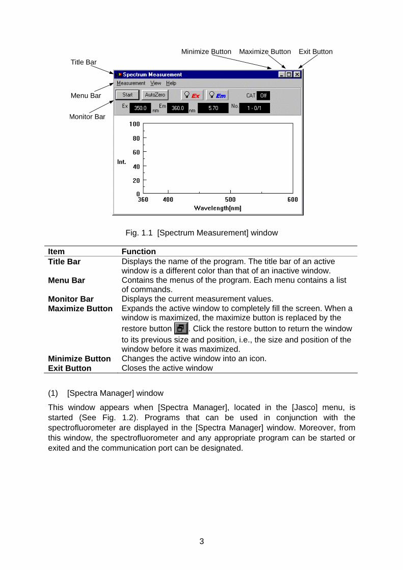
1.4 The Spectrofluorometer Software Features This section describes the locations and functions of various parts of the windows used in the Spectrofluorometer software. The [Spectrum Measurement] window is used as an example.
2
Title Bar
Menu Bar
Monitor Bar
Exit ButtonMaximize ButtonMinimize Button
Fig. 1.1 [Spectrum Measurement] window
Item Function Title Bar Displays the name of the program. The title bar of an active
window is a different color than that of an inactive window. Menu Bar Contains the menus of the program. Each menu contains a list
of commands. Monitor Bar Displays the current measurement values. Maximize Button Expands the active window to completely fill the screen. When a
window is maximized, the maximize button is replaced by the restore button . Click the restore button to return the window to its previous size and position, i.e., the size and position of the window before it was maximized.
Minimize Button Changes the active window into an icon. Exit Button Closes the active window
(1) [Spectra Manager] window
This window appears when [Spectra Manager], located in the [Jasco] menu, is started (See Fig. 1.2). Programs that can be used in conjunction with the spectrofluorometer are displayed in the [Spectra Manager] window. Moreover, from this window, the spectrofluorometer and any appropriate program can be started or exited and the communication port can be designated.
3

Fig. 1.2 [Spectra Manager] window
(2) The [Quantitative Analysis] application
The following three windows can be displayed using the [Quantitative Analysis] application (See Fig. 1.3). [Calibration Curve] Displays a calibration curve. Always displays when the
[Method Information] window is opened. [Data Sheet] Opening this window measures an unknown sample. The
[Calibration Curve] and [Method Information] windows must be opened in order to display this window.
[Method Information] Displays information concerning the measurement
currently being performed, including measurement parameters, calibration curve data, and comments. Always displays when the [Calibration Curve] window is opened.
These three windows may be opened simultaneously; however, no more than one window of each type may be opened at any given time.
4
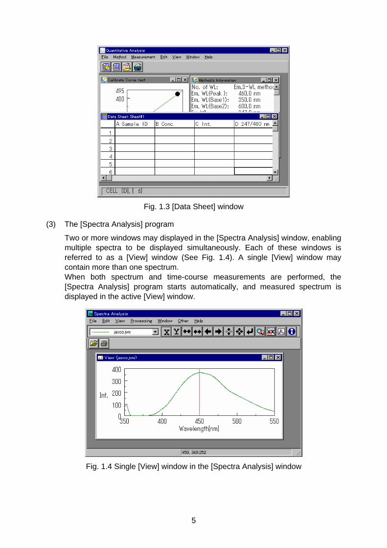
Fig. 1.3 [Data Sheet] window
(3) The [Spectra Analysis] program
Two or more windows may displayed in the [Spectra Analysis] window, enabling multiple spectra to be displayed simultaneously. Each of these windows is referred to as a [View] window (See Fig. 1.4). A single [View] window may contain more than one spectrum. When both spectrum and time-course measurements are performed, the [Spectra Analysis] program starts automatically, and measured spectrum is displayed in the active [View] window.
Fig. 1.4 Single [View] window in the [Spectra Analysis] window
5

2. Start-up and shut-down procedures and [Spectra Manager] This chapter describes the start-up and shut-down procedures for the Spectrofluorometer, the PC, applications for use with the Spectrofluorometer and [Spectra Manager].
2.1 Start-up procedures The following sections describe the start-up procedures for the Spectrofluorometer and the PC.
2.1.1 Turning on the Spectrofluorometer
Turn the power switch of the spectrofluorometer to the ON position.
“POWER” Switch Fig. 2.1 Power switch location
When the power to the spectrofluorometer is turned on, the power lamp of the spectrofluorometer is illuminated. The light source of the spectrofluorometer requires approximately five minutes to stabilize, after which measurement may be performed.
2.1.2 Turning on the PC and Windows start-up
Turn the power switches of the PC and monitor to their respective On positions. For information concerning Windows start-up procedures, refer to the Windows instruction manual.
2.2 Shut-down procedures This section describes the shut-down procedures the Spectrofluorometer and the PC.
2.2.1 Turning off the Spectrofluorometer and PC
(1) Turn the power switches of the PC and the monitor too the OFF position. Be careful not forget to turn off the monitor.
(2) Confirm that the sample chamber is empty and then turn the power switch to the spectrofluorometer to the OFF position.
6

(3) Allow the light source to cool for approximately five minutes and then place the dust cover over the spectrofluorometer.
2.3 [Spectra Manager] [Spectra Manager] is a menu application that is used to start spectra measurement and analysis and environment setting using the spectrofluorometer, and selecting, for starting up and shutting down the spectrofluorometer, as well as for setting the communication port.
Fig. 2.2 [Spectra Manager] window
Fig. 2.2 shows the standard [Measurement] and [Analysis] program menu. When additional programs are installed, they are added to this menu. The [Analysis] menu appears on the left and the [Measurement] menu appears on the right. To start a program, double-click on the program in the menu. If the spectrofluorometer has not already been started, both the program and spectrofluorometer will start simultaneously.
2.3.1 [Spectra Manager] start-up procedures
(1) At Windows start-up, the [Jasco]-[Spectra Manager] is activated. (See Fig. 2.3.) The [Spectra Manager] window, shown in Fig. 2.4, will appear.
Fig. 2.3 Starting [Spectra Manager] from the Start menu
7

Fig. 2.4 [Spectra Manager] window
Note: The [Spectra Manager] window displays all applications appropriate for use in conjunction with the Spectrofluorometer. The [Spectra Manager] window shown in Fig.2.4 lists the standard applications available for use in conjunction with the Spectrofluorometer. In addition to the standard applications, any optional applications that have been installed in the [Spectra Manger] will also appear in this window. Refer to Section 2.3.
(2) From the application list, simply double-click on the desired application to select it. The selected application starts, and the corresponding application window is displayed. The spectrofluorometer also starts automatically. The spectrofluorometer requires approximately two minutes to warm-up. Messages describing the start-up activities of the instruments appear throughout the procedure. For example, when the [Quantitative Analysis] program is started, the initialization screen shown in Figure 2.5 is displayed briefly, followed by the [Quantitative Analysis] window, shown in Fig. 2.6.
Note: Refer to chapter 3 ([Quantitative Analysis Introduction]) for a full description of the [Quantitative Analysis] program.
Fig. 2.5 Initialization window displayed during start-up
8

Fig. 2.6 [Quantitative Analysis] window
2.3.2 [Application] menu
This menu is used to start-up and exit [Measurement] and [Analysis] programs.
Fig. 2.7 [Application] Menu
2.3.2.1 [Analysis]
Starts the currently selected [Analysis] program.
Note: Analysis programs can also be started by double clicking on the appropriate menu item.
2.3.2.2 [Measurement]
Starts the currently selected [Measurement] program.
Note: Measurement programs can also be started up by double clicking on the appropriate menu item.
2.3.2.3 [Exit]
Exits the [Spectra Manager] window and returns to Windows.
9

2.3.3 [Instruments] menu
This menu is used to start and stop hardware, set the communication port, and show the instrument version information.
Fig. 2.8 [Instruments] menu
2.3.3.1 [Start]
Initializes the spectrofluorometer and begins communication with the spectrofluorometer. Initialization takes approximately two minutes. Normally, this operation is not necessary because the spectrofluorometer starts automatically when the [Measurement] program is started.
2.3.3.2 [Stop]
Stops communication with the spectrofluorometer. Normally, this operation is not necessary because communication with the spectrofluorometer stops automatically when the [Measurement] program is exited. 2.3.3.3 [Port Setting...] Changes the communication port designated for the spectrofluorometer. [COM1] is the default serial port for the Spectrofluorometer.
Fig. 2.9 [Port Setting] dialog box
The communication port can be changed by selecting a port from the list of [Ports] and then clicking <OK>.
2.3.3.4 [About...]
Displays the version information for the control driver of the spectrofluorometer.
10

Fig. 2.10 Control driver version information
2.3.4 [Help]
Displays the version information for [Spectra Manager].
Fig. 2.11 [Help] menu
2.4 Exiting measurement or analysis programs [Measurement] or [Analysis] programs can be exited using the following procedure:
(1) Select [Exit] from the [File] menu. If data exists which has been changed or has not been saved, a dialog box asking whether you would like to save the data will be displayed. Read the message and answer the question by clicking the appropriate button.
Note: This dialog box will vary. For newly created unsaved calibration curve data (quantitative analysis method), the following dialog box will be displayed.
Fig. 2.12 Quantitative analysis program exit dialog box
Click the <Yes> button to save the data. The [Save] dialog box will be displayed. Provide a name and then save the file. After the data has been saved, [Spectra Manager] returns to the [Spectra Manager] window.
Click the <No> button to exit the current program without saving the data. [Spectra Manager] returns to the [Spectra Manager] window.
11

(2) Select [Application]-[Exit] to close the [Spectra Manager] window and exit [Spectra Manager].
(3) Exit Windows
12

3. Quantitative Analysis and Spectrum Measurement This chapter describes quantitative analysis, spectrum measurement and various aspects of standard analysis. Parameter description is described here only briefly in order to provide a clear picture of the operation flow. Follow the procedures outlined below to familiarize yourself with these programs. For more detailed information, refer to the respective sections for each of these program.
3.1 Introduction to Quantitative Analysis The following sections briefly describe the [Quantitative Analysis] program and its operation flow. In addition, the procedures for creating calibration curves, performing measurement of an unknown sample, and saving and printing results are presented here.
3.1.1 Quantitative analysis program overview
3.1.1.1 Quantitative analysis program
In this [Quantitative Analysis] program, in addition to the standard single wavelength mode (i.e., one wavelength of excitation, one wavelength of emission), the emission mode or the excitation mode can be selected.
Emission mode: Enables measurement of the emission spectrum using a fixed Ex wavelength.
Excitation mode: Enables measurement of the excitation spectrum using a fixed Em wavelength.
One, two or three wavelengths can be selected depending the condition of the sample. Figure 3.1 illustrates the three possible methods of quantitative analysis.
Note: The emission mode and the excitation mode are ineffective when measuring in the standard single wavelength mode.
Fig. 3.1 Quantitative analysis methods
13
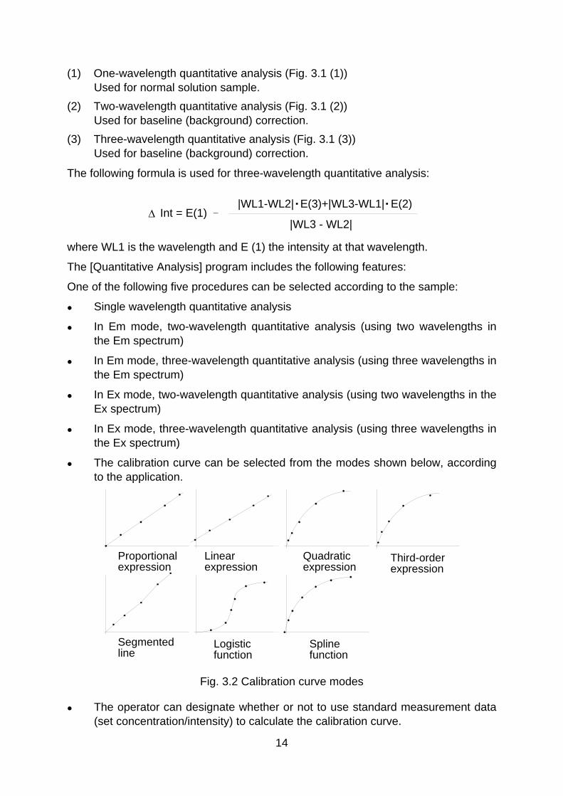
(1) One-wavelength quantitative analysis (Fig. 3.1 (1)) Used for normal solution sample. (2) Two-wavelength quantitative analysis (Fig. 3.1 (2)) Used for baseline (background) correction. (3) Three-wavelength quantitative analysis (Fig. 3.1 (3)) Used for baseline (background) correction.
The following formula is used for three-wavelength quantitative analysis:
Δ Int = E(1)
|WL3 - WL2|-
|WL1-WL2| E(3)+|WL3-WL1| E(2)・・
where WL1 is the wavelength and E (1) the intensity at that wavelength.
The [Quantitative Analysis] program includes the following features:
One of the following five procedures can be selected according to the sample:
Single wavelength quantitative analysis
In Em mode, two-wavelength quantitative analysis (using two wavelengths in the Em spectrum)
In Em mode, three-wavelength quantitative analysis (using three wavelengths in the Em spectrum)
In Ex mode, two-wavelength quantitative analysis (using two wavelengths in the Ex spectrum)
In Ex mode, three-wavelength quantitative analysis (using three wavelengths in the Ex spectrum)
The calibration curve can be selected from the modes shown below, according to the application.
Segmentedline
Logisticfunction
Splinefunction
Proportional expression
Linear expression
Quadraticexpression
Third-orderexpression
Fig. 3.2 Calibration curve modes
The operator can designate whether or not to use standard measurement data (set concentration/intensity) to calculate the calibration curve.
14

3.1.1.2 Quantitative analysis operation Start quantitative analysis program See Section 3.1.2 ↓ Create file ↓ Designate quantitative analysis method and measurement parameters ↓ Designate calibration curve parameters and input standard sample concentration See Section 3.1.3 ↓ Measure standard sample blank ↓ Measure standard samples ↓ Display calibration curve ↓ Modify (check and correct) calibration curve See Section 3.1.4 ↓ Save calibration curve See Section 3.1.5 ↓ Measure unknown samples See Section 3.1.6 ↓ Save results See Section 3.1.7 ↓ Print Results See Section 3.1.8 ↓ Exit quantitative analysis program See Section 3.1.9
3.1.2 Program startup
Double click [Quantitative Analysis] from the [Spectra Manager] window.
Fig. 3.3 [Spectra Manager] window
15

The message "Initializing…” will appear. During initialization, measurement parameters are transferred to the spectrofluorometer. When the transfer is complete, the program starts and the following window appears.
Fig. 3.4 [Quantitative analysis] window
3.1.3 Calibration curve creation
(1) Select [File] - [New...]. The following dialog box appears.
Fig. 3.5 [Open Parameters] dialog box
(2) Click <New> to open the following dialog box.
16

Fig. 3.6 [Quantitative Measurement Parameters] dialog box
(3) Changing measurement parameters
The [Quantitative Measurement Parameters] dialog box displays the instrument default settings. The following parameters may be changed.
Response : 1 sec Method : three-wavelength Mode : Emission Excitation wavelength : 247 nm Emission wavelength : Peak=460 nm, Base 1=350 nm, Base 2=600 nm Note: See Section 3.1.1.1 for a detailed description of quantitative analysis.
1) Click the arrow key to display the [Response] drop-down list. Then click [1 sec] to set the response to one second.
Change any other parameters as required. 2) Click [3 wavelength] in the wavelength group. The selected option button is
darkened (•). 3) Click the [Emission] option button in the mode group. The text field for entering
the wavelength of emission and the three text fields for entering Peak, Base 1 and Base 2 appear.
4) Use the keyboard to enter 247 in the Ex wavelength text field. Enter 460 in the Em wavelength Peak text field. Enter 350 and 600 in the Base 1 and Base 2 text fields, respectively.
(4) Click <OK> to transfer the measurement parameters to the spectrofluorometer. When transfer is complete, the [Calibration Curve Parameters] dialog box appears. The calibration curve parameters can be designated and the concentration of the standard sample can be specified from this dialog box.
17

Fig. 3.7 Dialog box indicating parameter transfer
Fig. 3.8 [Calibrate Curve Parameters] dialog box
(5) Setting calibration curve parameters
1) Set [Calib. curve] to [Proportional] using the same procedure as that used to change the measurement parameters.
2) If [Standard blank] is known, input that value in the text field. If [Standard blank] is unknown, it will be measured later, in which case, Steps 2) and 3) are not necessary.
3) Click on the [Enable Blank] checkbox to select it. (6) Inputting concentration
1) Click on the [Std#01] line of the standard data display field. The cursor will move to that line.
2) Input the concentration in the [Conc.] text field of the [Calibration Data Setting] group and then click <Append>. The concentration will appear in the standard data display field and the cursor will moves to the next line automatically.
Note: If the intensity of the standard sample is known, measuring the standard
sample is not necessary. Input the appropriate intensity, select the [Enable Calib. Data] checkbox, and then click <Append>.
3) Repeat Step 2) for each standard sample. 4) Click on the [Std#01] line in the data display field. The cursor will return to line 1.
(7) Click <Start...>. The [Quantitative Measurement] dialog box will open, and the standard blank and standard samples will be measured.
18

Note: When the [Quantitative Measurement] dialog box appears, it will cover the [Calibration Curve Parameters] dialog box. To view the [Calibration Curve Parameters] dialog box, click and drag the title bar of the [Quantitative Measurement] dialog box until the [Calibration Curve Parameters] dialog box is visible. Both of these dialog boxes will be active. The calibration curve parameters can be changed according to the procedures described in Steps (5) and (6).
Fig. 3.9 [Quantitative Measurement] dialog box
(8) Shutter confirmation
Click the button (Ex shutter button) or the button (Em shutter button). The yellow lamp icon on the Em shutter button indicates that the Em shutter is open.
Note: Before measurement, always confirm whether the shutters are open or closed.
The shutters are used to protect the detector and prevent sample decomposition. The Ex shutter should remain closed until starting measurement in order to prevent sample decomposition due to the light source.
(9) Measuring the standard blank
1) Select the [Blank] option button. 2) Place the standard blank in the cell holder of the sample chamber. The sample
cell holder is located at the right-front corner of the Spectrofluorometer.
19

Sample chamber
Fig. 3.11 Sample chamber
3) Click <Start> to measure the standard blank. The value will automatically appear in the [Standard Blank] text field of the [Calibration Curve Parameters] dialog box and the [Enable Blank] checkbox will be selected.
Note: When <OK> is clicked and the [Calibration Curve Parameters] dialog box is
closed, the standard blank value will be subtracted from the intensity value of the standard sample. Therefore, the standard blank and standard sample can be measured in any order.
(10) Standard samples measurement
Before measuring the standard samples, make sure that the cursor is positioned at the first line of the standard data display field. Click on the [Std#01] line to move the cursor to the first line.
1) Select the [Standard] option button. 2) Place the first standard sample in the cell holder. 3) Click <Start> to measure the standard sample. The intensity value appears
automatically in the standard data display field of the [Calibration Curve Parameters] dialog box. The [Use?] field will be changed from [---] to [Use], and the cursor automatically moves to the next line.
Note: The standard blank value is not subtracted from the intensity in the standard
data display field.
4) Repeat Steps 2) and 3) for each sample. 5) After standard sample measurement, click <Close> to close the [Quantitative
Measurement] dialog box. (11) Displaying the calibration curve
Click <OK> in the [Calibration Curve Parameters] dialog box. The standard blank value is subtracted from the intensity value of the standard sample and the [Calibration Curve] window opens. At the same time, the [Method Information] and [Data sheet] windows will be opened.
20

Note: If a calibration curve is created by selecting [Method] - [New], only the [Calibration Curve] and [Method Information] windows will be opened.
Fig. 3.12 [Data Sheet] window
3.1.4 Calibration curve modification
Click the title bar of the [Calibration Curve] window. This activates the [Calibration Curve] window, and the calibration curve can be confirmed. If the calibration curve must be changed, select [Method] - [Modify...]. The [Calibration Curve Parameters] dialog box will open (See Fig. 3.8).
Thus, the calibration curve parameters can be changed, and the standard samples can be re-measured. In addition, data can be invalidated rather than continuing to perform measurement.
Note: The calibration curve cannot be modified after measuring an unknown sample.
(1) Re-measurement
1) Move the cursor to the incorrect data line. 2) Click <Start...> to open the [Quantitative Measurement] dialog box. Repeat
standard sample measurement. (2) Invalidating
1) Move the cursor to the incorrect data line. 2) Deselect the [Enable Calib. Data] checkbox, and then click <Append>. The
[Use?] field will be changed from [Use] to [---].
3.1.5 Saving a quantitative analysis method
The quantitative analysis method (calibration curve data) and the measurement parameters can be saved on disk.
(1) Select [Method] - [Save As...]. The following dialog box will appear.
21

Fig. 3.13 [Save Parameters] dialog box
(2) Input a filename in the [Parameter Name] text field. The filename may contain up to 32 characters. A maximum of 32 calibration curve files may be input.
Note: Click <Comment...> to open the [Comments] dialog box. Sample name, operator, and organization can be recorded for future reference.
(3) Click <OK> to save the quantitative analysis method.
3.1.6 Unknown sample measurement
(1) Select [Measurement] - [Measurement...]. The following dialog box will appear.
Fig. 3.14 [Quantitative Measurement] dialog box
Note: Before measurement, click the <Shutter> button and confirm that both shutters are open on the emission and excitation sides. (See Item (8) in Section 3.1.3 for details.) In order to prevent sample decomposition due to the light source keep the Ex shutter closed until starting measurement.
(2) Sample blank measurement
Measure the sample blank according to the following procedure. The sample blank value can be confirmed by selecting [Measurement] - [Blank Correction].
Note: If the sample blank is not measured, the standard sample blank value is used as the sample blank value.
1) Select the [Blank] option button. 2) Place the sample blank in the cell holder of the sample chamber. 3) Click <Start>. The sample blank will be measured. The results of measurement
22

will appear on the [Data Sheet]. (3) Sample measurement
1) Select the [Sample] option button. 2) Place the sample in the cell holder 3) Click <Start>. The sample will be measured and the concentration will be
calculated from the calibration curve displayed in the window. The results will appear on the [Data Sheet].
4) Repeat Steps 2) and 3) for each sample. Note: The sample blank is subtracted from the intensity of the sample when
calculating concentration. The sample blank can be re-measured during sample measurement. The blank value is valid for subsequent sample measurements.
<<Re-measurement>>
To re-measure a sample, move the cursor to the desired line in the [Data Sheet] window and repeat the measurement. The previous data will be overwritten automatically. Following sample re-measurement, measurement will resume at the next sample. In order to resume measurement at a specific sample number, one of the following procedures must be performed.
• Close the [Quantitative Measurement] dialog box before measurement. Select [Measurement] - [Parameters...] to open the [Quantitative Measurement - Parameters] dialog box and input the desired sample number.
• After measurement, rewrite the data using the data sheet modifying function (See Section 4.4).
Note: The line containing the incorrect measurement can be invalidated (See Section 4.4.4).
3.1.7 Saving a data sheet
Data sheets and quantitative analysis methods can be saved on disk.
(1) Select [File] - [Save As...] to open the following dialog box.
Fig. 3.15 [Save As] dialog box
23

Note: Click <Comments...> to open the [Comments] dialog box. Sample name, operator, and organization can be recorded for future reference.
(2) Select the target directory from the [Save in:] drop-down list. (3) Set [Save as Type] to [JASCO Qnt.(*.JQA)].
(4) Enter a filename in the [File name] text field. The file extension is not required. (The file extension is the part of the name that appears after the ".")
(5) Click <Save> to save the data sheet.
3.1.8 Printing results
Quantitative analysis data can be printed.
(1) Select [File] - [Print Setup...]. The following dialog box will appear. Click <OK> to confirm the printer settings.
Note: The content of the dialog box varies according to the printer.
Fig. 3.17 [Print Setup] dialog box
(2) Select [File] - [Page Setup...]. The following dialog box will appear. Select the items that you wish to print and click <OK> to confirm the selected items. The dialog box will close.
Fig. 3.18 [Print Format] dialog box
(3) Select [File] - [Print]. The following dialog box will appear.
Note: The content of the dialog box varies according to the printer.
24

Fig. 3.19 [Print] dialog box
(4) Click <OK> to print the quantitative analysis data.
3.1.9 Exiting quantitative analysis
Select [File] - [Exit] to return to the [Spectra Manager] window after measurement is complete.
Note: If unsaved [Data Sheet] and/or [Calibration Curve] data exist, a message will appear asking whether the data should be saved. Answer the question by clicking the appropriate button.
25

3.2 Spectrum Measurement and Spectra Analysis Introduction This section describes the procedures for starting the [Spectrum Measurement] program, measuring samples, saving measured spectra, and printing data. This section also outlines the procedures for peak find, and peak display style change in the [Spectra Analysis] program.
3.2.1 Spectrum measurement and spectra analysis overview
3.2.1.1 Spectrum measurement and spectra analysis
A. [Spectrum Measurement] program
This instrument measures the following five types of spectra:
(1) Fluorescent emission spectrum (or simply "emission" or "Em" spectrum)
Fluorescence is generally emitted in the wavelength region that is longer than the wavelength of excitation. The emission spectrum is defined as the spectrum obtained by exciting the sample and scanning the Em monochromator over the selected range on the side having longer wavelength than that set (at a fixed point) for the wavelength of excitation.
(2) Fluorescent excitation spectrum (or simply "excitation" or "Ex" spectrum)
The excitation spectrum is defined as the spectrum obtained by scanning the Ex monochromator over the selected range on the side having shorter wavelength than that set (at a fixed point) for the wavelength of emission. Correcting the excitation spectrum should yield a spectrum similar to the absorption spectrum.
(3) Emission synchronous spectrum (or simply "synchronous" or "Sync" spectrum)
The synchronous spectrum is defined as the spectrum obtained by scanning the wavelengths of the Em and Ex monochromators while maintaining the same difference between the two wavelengths. This type of spectrum is particularly useful in the quantitative analysis of multi-component samples.
(4) Excitation single-beam spectrum (or simply "Ex single" spectrum)
The Ex single spectrum represents the measurement of the waveform dispersion of excitation intensity. The measurement results show the characteristics of the light source and Ex monochromator independent of the Em monochromator. In other words, this measurement is used to determine the energy of the Ex monochromator.
(5) Emission single-beam spectrum (or simply "Em single" spectrum)
The Em single spectrum represents the measurement of the wavelength dispersion of light incident on the Em monochromator. The wavelength characteristics of the Em monochromator can be checked by introducing zero-order light from the Ex monochromator, setting a diffuser in the sample chamber, and then measuring the Em single spectrum. Likewise, the Em spectrum can be measured by closing the shutter of the Ex monochromator and placing a chemiluminescent sample in the sample chamber.
The spectrum measurement mode can be changed in the spectrum measurement
26

program by changing the [Measurement Mode].
Spectra cannot be printed or saved in the [Spectrum Measurement] program. Spectrum measurement automatically starts the [Spectra Analysis] program and the spectra are displayed in the active view. Spectra can be saved or printed using the [Spectra Analysis] program.
Note: In the Spectra Analysis program, the window for displaying spectra (or time-course data) is called the "view".
Multiple views can be opened simultaneously. Multiple spectra (or time-course data) can be loaded into one view.
B. [Spectra Analysis] program
The main functions of the [Spectra Analysis] program are listed below.
(1) File functions: Save, load or print spectra.
(2) Edit functions: Copy a spectrum to the clipboard or to another view or delete a spectrum.
(3) View functions: Change spectrum characteristics such as scale, color, or font. Designate whether or not to display peak find results.
(4) Data processing functions: Correction Baseline correction: Corrects a spectrum using a designated baseline. Smoothing: Smoothes a spectrum. Noise elimination Eliminates noise of unknown cause. Deconvolution Separates overlaid peaks. FFT filter Eliminates noise. Data Cut Cuts unnecessary data. Arithmetic Arithmetic: Performs arithmetic operations between spectra or
between a spectrum and a constant. Derivative: Differentiates a spectrum. KK conversion Performs Kramers-Kronig conversion. Peak Peak find: Finds spectrum peaks (or valleys). Peak height: Calculates peak height and peak height ratio. Peak area: Calculates peak area and peak area ratio. Peak width: Calculates full width at half-peak. Subtraction: Calculates a difference spectrum. X-unit conversion: Converts X axis unit. Y-unit conversion: Not used. Other Comment Edits comments. Common option Kinetics Calculates enzyme activity.
27
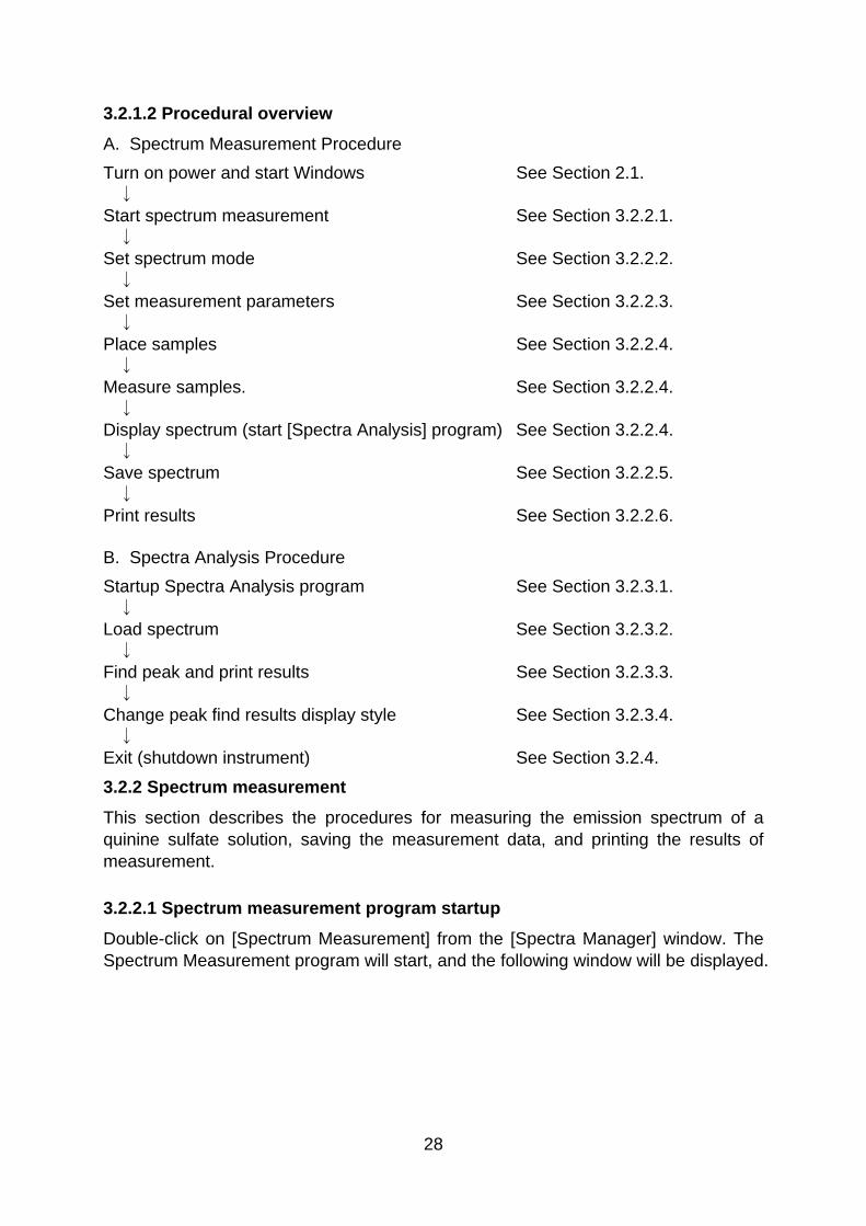
3.2.1.2 Procedural overview
A. Spectrum Measurement Procedure Turn on power and start Windows See Section 2.1. ↓ Start spectrum measurement See Section 3.2.2.1. ↓ Set spectrum mode See Section 3.2.2.2. ↓ Set measurement parameters See Section 3.2.2.3. ↓ Place samples See Section 3.2.2.4. ↓ Measure samples. See Section 3.2.2.4. ↓ Display spectrum (start [Spectra Analysis] program) See Section 3.2.2.4. ↓ Save spectrum See Section 3.2.2.5. ↓ Print results See Section 3.2.2.6. B. Spectra Analysis Procedure Startup Spectra Analysis program See Section 3.2.3.1. ↓ Load spectrum See Section 3.2.3.2. ↓ Find peak and print results See Section 3.2.3.3. ↓ Change peak find results display style See Section 3.2.3.4. ↓ Exit (shutdown instrument) See Section 3.2.4.
3.2.2 Spectrum measurement
This section describes the procedures for measuring the emission spectrum of a quinine sulfate solution, saving the measurement data, and printing the results of measurement.
3.2.2.1 Spectrum measurement program startup
Double-click on [Spectrum Measurement] from the [Spectra Manager] window. The Spectrum Measurement program will start, and the following window will be displayed.
28

Fig. 3.20 [Spectrum Measurement] window
Select the [Measurement] menu to display the following menu.
Fig. 3.21 [Measurement] menu
The following operations can be performed from this menu: [Start] Starts spectrum measurement [Parameter...] Sets measurement parameters [Move Wavelength...] Moves the spectrofluorometer wavelength to a designated
wavelength [Autozero] Sets measurement value at the current wavelength to 0 [Shutter Control] Opens/closes the shutter [Exit] Exits the spectrum measurement program and returns to
the [Spectrum Manager] window
3.2.2.2 Setting spectrum measurement mode
The spectrum measurement mode is changed by opening the [Parameters] dialog box and selecting the desired [Measurement Mode]. Changing the measurement mode rewrites various parameter settings.
(1) Select [Measurement] - [Parameters...]. The following dialog box will be displayed.
29
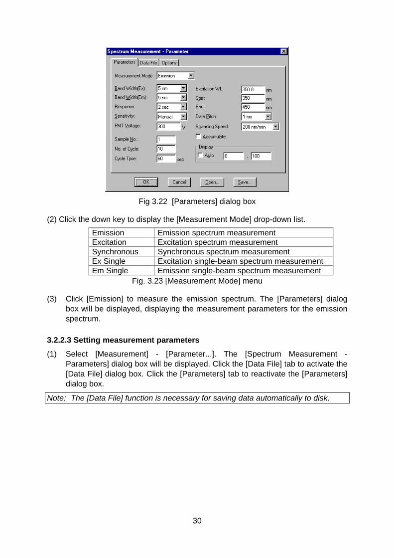
Fig 3.22 [Parameters] dialog box
(2) Click the down key to display the [Measurement Mode] drop-down list.
Emission Emission spectrum measurement Excitation Excitation spectrum measurement Synchronous Synchronous spectrum measurement Ex Single Excitation single-beam spectrum measurement Em Single Emission single-beam spectrum measurement
Fig. 3.23 [Measurement Mode] menu
(3) Click [Emission] to measure the emission spectrum. The [Parameters] dialog box will be displayed, displaying the measurement parameters for the emission spectrum.
3.2.2.3 Setting measurement parameters
(1) Select [Measurement] - [Parameter...]. The [Spectrum Measurement - Parameters] dialog box will be displayed. Click the [Data File] tab to activate the [Data File] dialog box. Click the [Parameters] tab to reactivate the [Parameters] dialog box.
Note: The [Data File] function is necessary for saving data automatically to disk.
30

Fig. 3.24 [Parameters] dialog box Fig. 3.25 [Data File] dialog box
(2) Procedure for changing measurement parameters.
The default parameters for the instrument are displayed in the [Parameters] dialog box. These parameters can be changed, as described in the following examples.
Response: 0.5 sec Excitation Wavelength: 247 nm Start: 350 nm End: 600 nm
1) Changing the response [Response] is a drop-down list box. Click the arrow to the right of the box to display the available modes. Click [Medium] to designate medium response.
2) Changing the excitation wavelength Click on the [Excitation Wavelength] text field. A cursor will be displayed in the text field. The excitation wavelength can then be entered using the numeric keys.
3) Changing the wavelength range Enter the shorter wavelength end in the [Start] text field and the longer wavelength end in the [End] text field. Change the other parameters as desired
(3) After changing the necessary parameters, click <OK> to transfer the parameters to the spectrofluorometer.
3.2.2.4 Sample measurement
(1) Shutter confirmation
Click the button (Ex shutter button) or the button (Em shutter button). The yellow lamp icon on the Em shutter button indicates that the Em shutter is open..
Note: Before measurement, always confirm whether the shutters are open or closed. The shutters are used to protect the detector and prevent sample decomposition. The Ex shutter should remain closed until starting measurement in order to prevent sample decomposition due to the light source.
31

(2) Place a sample in the cell holder of the sample chamber, and then close the lid.
Sample chamber
Fig. 3.26 Sample chamber
(2) Select [Measurement] - [Start] (or click the <Start> button). The sample is measured and the measurement progression will be displayed. When measurement is complete, the [Spectra Analysis] program starts automatically and the spectrum is displayed in the active view.
Fig. 3.27 Spectrum View (Spectra Analysis)
Note: After starting spectra analysis and performing the initial measurement, [Spectrum View] showing the results of the most recent measurement will be displayed over the previously displayed [Spectrum View], which will no longer be visible. To keep the previous [Spectrum View], save or print it. To redisplay the hidden [Spectrum View], change the application.
32
3.2.2.5 Spectrum save
Spectra can be saved in a file.
Note: Save spectra when the [Spectra Analysis] program is active.
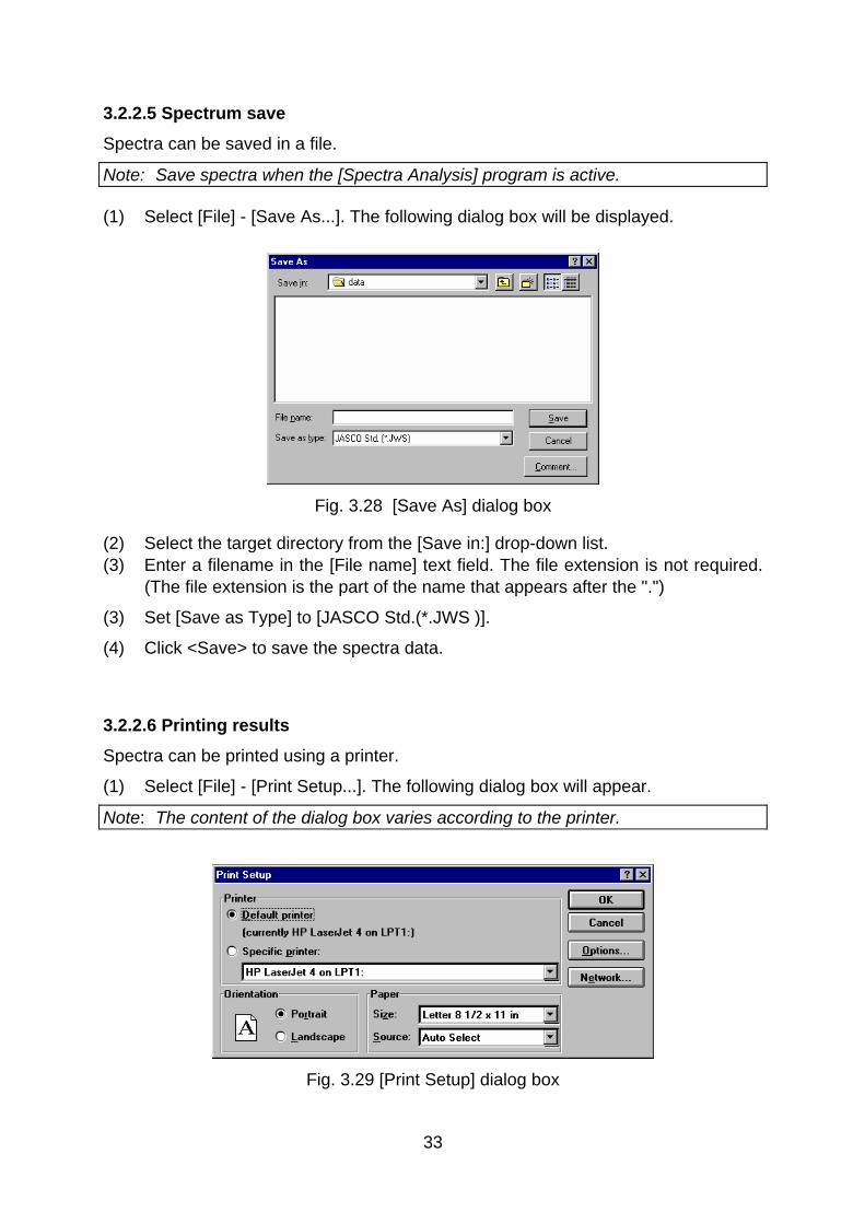
(1) Select [File] - [Save As...]. The following dialog box will be displayed.
Fig. 3.28 [Save As] dialog box
(2) Select the target directory from the [Save in:] drop-down list. (3) Enter a filename in the [File name] text field. The file extension is not required.
(The file extension is the part of the name that appears after the ".")
(3) Set [Save as Type] to [JASCO Std.(*.JWS )].
(4) Click <Save> to save the spectra data.
3.2.2.6 Printing results
Spectra can be printed using a printer.
(1) Select [File] - [Print Setup...]. The following dialog box will appear.
Note: The content of the dialog box varies according to the printer.
Fig. 3.29 [Print Setup] dialog box
33
(2) Select [File] - [Print...]. The following dialog box will appear. The content of the dialog box varies according to the active printer.
Fig. 3.30 [Print] dialog box
(3) Click <OK> to print the spectra.
3.2.3 Spectra analysis operation
The [Spectra Analysis] program saves and prints spectra according to the procedures described previously, processes data such as peak find, derivative and subtraction, changes the display settings, including scale, color and line style, and performs other functions related to spectral analysis.
This section describes the procedures for storing saved spectra, executing peak find, and printing the peak find results. In addition, the method for changing the display style and displaying the peak find results is described.
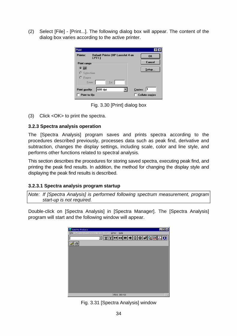
3.2.3.1 Spectra analysis program startup
Note: If [Spectra Analysis] is performed following spectrum measurement, program start-up is not required.
Double-click on [Spectra Analysis] in [Spectra Manager]. The [Spectra Analysis] program will start and the following window will appear.
Fig. 3.31 [Spectra Analysis] window
34

3.2.3.2 Loading spectra
Saved spectra can be loaded into the memory of the [Spectra Analysis] program.
(1) Select [File] - [Open...]. The following dialog box will be displayed.
Fig. 3.32 [Open] dialog box
(2) In the [File Name] list, click on the name of the file saved, as described in Section 3.2.2.5.
(3) Click <Open> to open a new view and display the designated spectrum.
Fig. 3.33 Spectrum View
3.2.3.3 Peak find and printing results
Peaks can be determined from the displayed spectrum.
(1) Select [Processing] - [Peak Process] - [Peak Find...]. The following dialog box will be displayed.
35
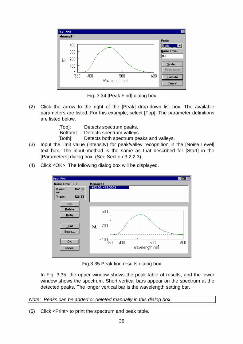
Fig. 3.34 [Peak Find] dialog box
(2) Click the arrow to the right of the [Peak] drop-down list box. The available parameters are listed. For this example, select [Top]. The parameter definitions are listed below.
[Top]: Detects spectrum peaks. [Bottom]: Detects spectrum valleys. [Both]: Detects both spectrum peaks and valleys. (3) Input the limit value (intensity) for peak/valley recognition in the [Noise Level]
text box. The input method is the same as that described for [Start] in the [Parameters] dialog box. (See Section 3.2.2.3).
(4) Click <OK>. The following dialog box will be displayed.
Fig.3.35 Peak find results dialog box
In Fig. 3.35, the upper window shows the peak table of results, and the lower window shows the spectrum. Short vertical bars appear on the spectrum at the detected peaks. The longer vertical bar is the wavelength setting bar.
Note: Peaks can be added or deleted manually in this dialog box.
(5) Click <Print> to print the spectrum and peak table.
36

(6) When printing is complete, click <OK>. The peak detection results are saved and the previous view will be displayed.
Note: The [View] does not change. However, the peak detection results can be displayed by changing the display settings. (See Section 3.2.3.4)
3.2.3.4 Peak detection results display
(1) Select [View] - [Peak]. The following menu will be displayed.
Fig. 3.36 Peak display menu
(2) A check mark is appended to [None]. Click [Bar, X, Y]. The check mark moves to [Bar, X, Y]. In this view mode, vertical bars appear, indicating the peak position, wavelength and fluorescence intensity, as shown below.
Fig. 3.37 Spectrum view (Peak Display)
Note: Clicking [None] in the peak display menu returns to the original View
37

3.2.4 Instrument shutdown
Refer to Section 2 for more information about instrument shut-down. This section provides only a brief description of the procedure.
3.2.4.1 Exiting spectrum measurement and spectra analysis
(1) Exiting the [Spectra Analysis] program
Select [File] - [Exit]. The [Spectra Analysis] window will close and the [Spectrum Measurement] window will be displayed.
Note: If an unsaved spectrum exists, a message will be displayed, informing the operator. Proceed according to the instructions provided in the message. A message will be displayed for each unsaved spectrum. Repeat the procedure accordingly.
(2) Exiting the [Spectrum Measurement] program
Select [Measurement] - [Exit]. The [Spectrum Measurement] window will close and the [Spectra Manager] window will be displayed.
(3) Exiting the [Spectra Manager] program
Select [Applications] - [Exit].
3.2.4.2 Exiting Windows and instrument shut-down
(1) Exiting Windows
Exit Windows according to the procedure described in the Windows User’s Guide.
(2) PC shut-down
Turn off power to both the PC and Display. In particular, be sure that the Display has been turned off.
(3) Spectrophotometer shut-down
Confirm that the sample chamber is empty, and then turn off the spectrophotometer. Wait approximately 5 minutes until the light source has cooled, and then cover the instrument.
38

4. [Quantitative Analysis] Program Reference Double-click on [Quantitative Analysis] in the [Spectra Manager] window. The [Quantitative Analysis] program starts, and the following window is displayed after spectrofluorometer initialization.
Fig, 4.1 [Quantitative Analysis] window
4.1 [File] menu
Data sheets can be created, saved, or printed from this menu. Select [File] to display the following menu.
Fig. 4.2 [File] menu
4.1.1 [New...]
Opens a new [Data Sheet] display.
Note: If an unsaved [Data Sheet] and/or [Calibration Curve] exists in the window when [New...] is selected, a message will be displayed asking the operator whether the data should be saved. Proceed according to the instructions provided in the message.
When [New...] is selected, the following dialog box will be displayed.
39 39
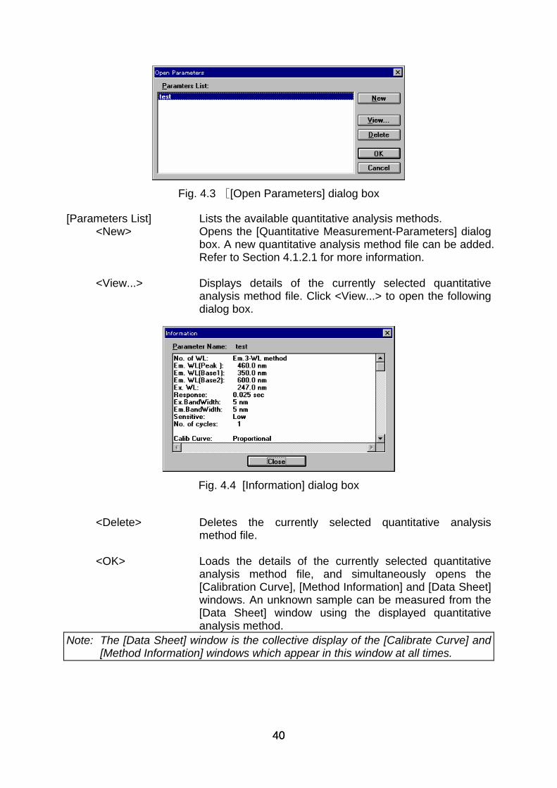
Fig. 4.3 [[Open Parameters] dialog box
[Parameters List] Lists the available quantitative analysis methods. <New> Opens the [Quantitative Measurement-Parameters] dialog
box. A new quantitative analysis method file can be added. Refer to Section 4.1.2.1 for more information.
<View...> Displays details of the currently selected quantitative
analysis method file. Click <View...> to open the following dialog box.
Fig. 4.4 [Information] dialog box
<Delete> Deletes the currently selected quantitative analysis
method file. <OK> Loads the details of the currently selected quantitative
analysis method file, and simultaneously opens the [Calibration Curve], [Method Information] and [Data Sheet] windows. An unknown sample can be measured from the [Data Sheet] window using the displayed quantitative analysis method.
Note: The [Data Sheet] window is the collective display of the [Calibrate Curve] and [Method Information] windows which appear in this window at all times.
40 40
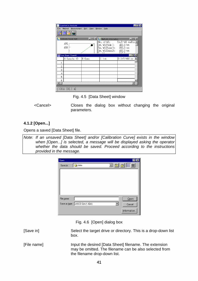
Fig. 4.5 [Data Sheet] window
<Cancel> Closes the dialog box without changing the original parameters.
4.1.2 [Open...]
Opens a saved [Data Sheet] file.
Note: If an unsaved [Data Sheet] and/or [Calibration Curve] exists in the window when [Open...] is selected, a message will be displayed asking the operator whether the data should be saved. Proceed according to the instructions provided in the message.
Fig. 4.6 [Open] dialog box
[Save in] Select the target drive or directory. This is a drop-down list box.
[File name] Input the desired [Data Sheet] filename. The extension
may be omitted. The filename can be also selected from the filename drop-down list.
41 41

[Save as type] Files must be saved as JQA files (These files will have the .JQA file extension).
[Information...] Displays information about the quantitative analysis file.
4.1.3 [Save]
Saves the active [Data Sheet] under the current filename. Measurement parameters and calibration curve data are also saved. Any previous data in the file is overwritten.
4.1.4 [Save As...]
Saves the active [Data Sheet] under a new filename. Measurement parameters and calibration curve data are also saved.
Fig. 4.7 [Save As] dialog box
[Save in] Select the target drive or directory. This is a drop-down list box.
[File name] Input the name of the [Data Sheet] file to be saved. If the
extension is omitted, the desired file type extension is affixed automatically. If the filename of an existing file is selected, the following dialog box will be displayed.
Fig. 4.8 Dialog box displayed when the filename of an existing file is selected
If the <OK> button is clicked, the original file will be overwritten.
42 42

File name list Lists all files saved in the target directory. Use this list as a reference when selecting filenames. Clicking on an existing filename displays that filename in the [File name] text box. The name can then be edited or selected as the file name for the new file.
[Save as type] File cannot be saved if an incorrect extension is input. [Comments...] Sample name, operator, organization and/or other
comments can be input or edited.
4.1.5 [Page Setup...]
Designates the contents that will be printed, e.g., [Data Sheet], calibration curve, or measurement parameters.
Fig. 4.9 [Print Format] dialog box
[Title] Title text box. A maximum of 62 characters may be input as a title for the document.
[Pattern] group Either the quantitative analysis method or results can be
printed by selecting either the [Method] or [Results] option button.
[Item] group Items such as [Parameters] and [Graph] can be selected
for printing from this group. A check in the checkbox indicates that the item will be printed.
F< ont...> button Opens the [Font] dialog box.
4.1.6 [Print Setup...]
Designates the target printer and printing settings.
Note: The content of the dialog box varies according to the printer.
43 43

Fig. 4.10 [Print Setup] dialog box
[Specific Printer] Lists the available printers. (Additional printers can be selected by adding them from the [Main] group control panel.
<Options…> button Used to change the print settings for the target printer. The
dialog box that is displayed varies according to the printer.
4.1.7 [Print...]
Prints the data from the active window designated by [Page Setup...].
Note: The content of the dialog box varies according to the printer.
Fig. 4.11 [Print] dialog box
[Select print range] Only [All pages] is available. [Print Quality] list Designates print quality. Cannot be designated for some
printers. The resolution of the printer is indicated in dpi, which indicates the number of dots per inch. The higher the dpi, the better the resolution.
[Printer Settings...] Designates the target printer and print settings for a printer.
The same procedure as that for [Printer Settings] is used.
4.1.8 [Exit]
Exits the quantitative analysis program and returns to the [Spectra Manager]. If an
44 44
unsaved [Data Sheet] and/or [Calibration Curve] exists, a message is displayed asking whether the operator wishes to save the information. Proceed according to the instructions provided in the message.
4.2 [Method] menu
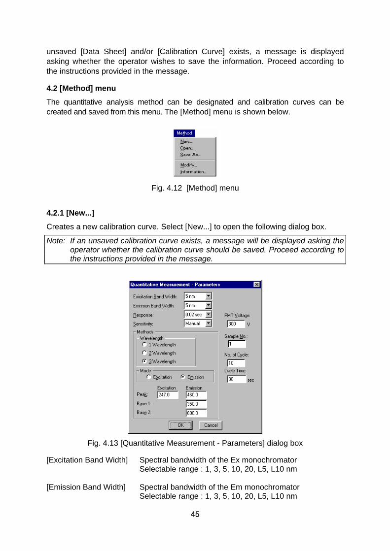
The quantitative analysis method can be designated and calibration curves can be created and saved from this menu. The [Method] menu is shown below.
Fig. 4.12 [Method] menu
4.2.1 [New...]
Creates a new calibration curve. Select [New...] to open the following dialog box.
Note: If an unsaved calibration curve exists, a message will be displayed asking the operator whether the calibration curve should be saved. Proceed according to the instructions provided in the message.
Fig. 4.13 [Quantitative Measurement - Parameters] dialog box
[Excitation Band Width] Spectral bandwidth of the Ex monochromator Selectable range : 1, 3, 5, 10, 20, L5, L10 nm [Emission Band Width] Spectral bandwidth of the Em monochromator Selectable range : 1, 3, 5, 10, 20, L5, L10 nm
45 45

[Response] Response speed Selectable range : 0.01, 0.02, 0.05, 0.1, 0.2, 0.5, 1, 2, 4, or 8 sec [Sensitivity] Change the set value of the photomultiplier tube voltage. Low, Medium, High, or Manual [PMT Voltage] Designates the Photomultiplier tube voltage([PMT voltage]
text box), Setting to Manual. Input rabge : 0 to 1000 V [Wavelength] The number of wavelengths used in quantitative analysis.
Selects the optimum number of wavelengths from 1-wavelength, 2-wavelength and 3-wavelength according to the sample condition.
• 1 wavelength (quantitative analysis method): Used for common solution sample (Fig. 4.14 (1)).
• 2 wavelength (quantitative analysis method): Performs baseline(background) correction (Fig. 4.14 (2)).
• 3 wavelength (quantitative analysis method): Performs baseline(background) correction (Fig. 4.14 (3)).
In [3-wavelength] analysis, the fluorescence intensity is obtained using the following equation :
Δ Int = E(1) |WL3 - WL2|
-|WL1-WL2| E(3)+|WL3-WL1| E(2)・・
WL 1 WL 1WL 2
ΔΔ
WL 1WL 2 WL 3
E(2)
E(1)
E(3)Int
Int
(Peak) (Peak) (Peak)(Base 1) (Base 1) (Base 2)
(1) 1-wavelength (2) 2-wavelength (3) 3-wavelength Fig. 4.14 Quantitative analysis methods
[Mode] In this quantitative analysis program, one of the following two modes (emission or excitation) can be selected in addition to the standard single-wavelength mode (i.e., one wavelength of excitation, one wavelength of emission). Emission mode: Enables measurement of the emission
spectrum with a fixed Ex wavelength. Excitation mode: Enables measurement of the excitation
spectrum a with fixed Em wavelength. One, two or three wavelengths can be selected depending
on the condition of the sample. Figure 4.14 illustrates the
46 46

three quantitative analysis methods. Note: The emission mode and excitation mode described above are ineffective when
measuring in the standard single-wavelength mode.
Enter the proper Ex wavelength to measure the Em spectrum; enter the proper Em wavelength to measure the Ex spectrum.
[Base 1] Base 1 wavelength (WL2) [Base 2] Base 2 wavelength (WL3) [Sample No.] Designates the sample number of the sample to be
measured. Sample number is incremented by one for each measurement.
Input range:1 to 999 [No. of Cycles] Designates how many times each sample is measured. If
two or more measurements are desired, the [Cycle Time] field will be displayed.
Input range:1 to 9999 [Cycle Time] Designates the time in seconds between measurements. If
the cycle time is shorter than the measurement time, the next measurement starts immediately.
Input range : 0 to 15000 sec. <OK> button Transfers the measurement parameters to the
spectrofluorometer, after which the [Calibration Curve Parameters] dialog box will be displayed.
Fig. 4.15 [Quantitative Measurement] dialog box
47 47

Fig. 4.16 [Calibrate Curve Parameters] dialog box
[Graph Setting] group [Calib Curve] Designates the type of calibration curve. Click the drop-down
format box and select the desired type of calibration curve. Figure 4.17 shows the names of modes and types of curves. Fig. 4.17 Calibration curve modes
[Standard Blank] If the standard blank value is known, enter the standard blank value. Doing so will place a checkmark in the [Enable Blank] checkbox. If the standard blank is unknown, leave the [Standard Blank] text box blank. The standard blank can be measured later from the [Quantitative Measurement] dialog box.
[Enable Blank] Select the [Enable Blank] checkbox when the standard
blank value is input. A checkmark will automatically be placed in the [Enable Blank] checkbox when the standard blank is measured from the [Quantitative Measurement] dialog box.
[Calibrate Data Setting] group [Number] Indicates the standard sample number. The displayed number
reflects the selected standard sample from the standard data display field. The concentration and intensity of the selected standard sample can be designated.
[Conc.] Text box for setting the standard sample concentration. [Int] Text box for setting the standard sample intensity, if known.
If the standard sample intensity is unknown, leave the [Int] text box blank. The standard sample intensity can be measured later from the [Quantitative Measurement] dialog box.
[Enable Calib. Data] Data in the standard data display field can be used for the
48 48

calibration curve by selecting the [Enable Calib. Data] checkbox. Select the checkbox (x), and then click the <Append> button. The column with [---] in the standard data display field is rewritten to [Use].
<Append> button Click the <Append> button to write into the standard data
display field the concentration and intensity settings in the [Calibrate Data Setting] group. If the [Enable Calib. Data] checkbox is selected, [---] in the standard data display field is rewritten to [Use].
Standard data display field Shows the input or measured standard data (concentration,
intensity). Data of the selected line can be input or measured. <Parameters...> button Click the <Parameters...> button to return to the
[Quantitative Measurement Parameters] dialog box. <Start...> button Click the <Start...> button to open the [Quantitative
Measurement] dialog box. The standard blank and standard sample are measured from this dialog box.
Fig 4.18 [Quantitative Measurement] dialog box
Ex Shutter button Em Shutter button
Click the button (Ex Shutter button) or the (Em Shutter button). The lamps on these buttons turn yellow to indicate that the corresponding shutter is open.
[Standard] Select the [Standard] option button to measure a standard
sample. [Blank] Select the [Blank] option button to measure a standard
blank. <Start> Starts measurement. When a standard sample is measured, the measurement
value is written to the [Int] column of the standard sample data display field in the [Calibration Curve Parameters] dialog box. At the same time, [---] is rewritten to [Use].
49 49

When a standard blank is measured, the measurement value is written to the [Standard Blank] text box and a checkmark is placed in the [Enable Blank] checkbox.
Note: The [Quantitative Measurement] and [Calibration Curve Parameters] dialog boxes are both active. To view the [Calibration Curve Parameters] dialog box, click and drag on the title bar of the [Quantitative Measurement] dialog box.
<Close> button Closes the [Quantitative Measurement] dialog box and returns to the [Calibration Curve Parameters] dialog box.
<Goto WL...> button Moves the wavelength of the spectrofluorometer to a
designated wavelength. When <Goto WL...> is selected, the following dialog box will be displayed.
Fig. 4.19 [Goto Wavelength] dialog box
[Excitation Wavelength] :Text box for inputting excitation wavelength. [Emission Wavelength] :Text box for inputting emission wavelength. <OK> button Click the <OK> button to accept and move the wavelength
of the spectrofluorometer to the designated wavelength. <Cancel> button Closes the dialog box without changing the previously
designated wavelength. <Auto Zero> button Sets the intensity of the current wavelength to zero. <OK> button Exits the [Calibration Curve Parameters] dialog box and
opens the [Calibration Curve] and [Method Information] windows.
50 50

Fig. 4.20 [Calibrate Curve] and [Method Information] windows
4.2.2 [Open...]
Opens saved quantitative analysis method files.
This function is equivalent to that described in Section 4.1.1.
4.2.3 [Save As...]
Saves quantitative analysis method data, including the calibration curve and measurement parameters.
Fig. 4.21 [Save Parameters] dialog box
[Parameter Name] Text box for inputting the quantitative analysis method filename. Up to 32 characters may be input. If an existing name from the [Quantitative analysis method name list] is designated, the previous file will be overwritten.
<OK> button Saves the quantitative analysis method. <Comments...> button Sample name, operator, copyright, and/or other
information can be input or edited. The following dialog box will be displayed.
51 51

Fig. 4.22 [Comments] dialog box
Input [Sample Name], [Operator], [Copyright] and/or [Comment]. The number of characters that can be input for each field is 62, 62, 62, and 124, respectively.
4.2.4 [Modify...]
Edits existing calibration curve data. When this function is selected, the [Calibration Curve Parameters] dialog box will be displayed. Refer to the [Calibration Curve Parameters] dialog box in Section 4.2.1.
Note: If an unsaved calibration curve exists, a message will be displayed to ask the operator whether it should be saved. Proceed according to the instructions provided in the message.
4.2.5 [Information...]
When the [Method Information] window is in icon form, Double-clicking the icon expands the window to its previous size.
Fig. 4.23 [Method Information] window
4.3 [Measurement] menu
The items in this menu are active only when the [Data Sheet] window is open.
52 52
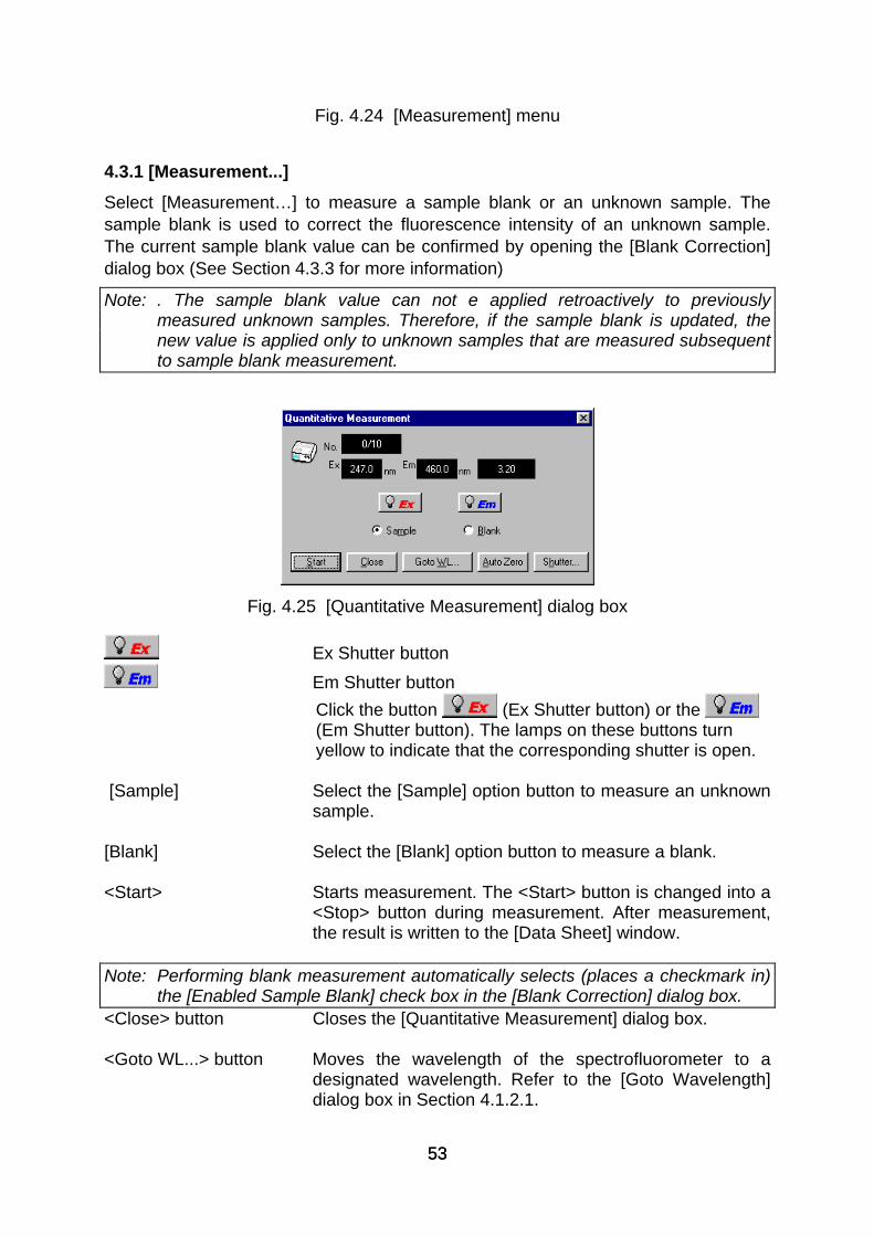
Fig. 4.24 [Measurement] menu
4.3.1 [Measurement...]
Select [Measurement…] to measure a sample blank or an unknown sample. The sample blank is used to correct the fluorescence intensity of an unknown sample. The current sample blank value can be confirmed by opening the [Blank Correction] dialog box (See Section 4.3.3 for more information)
Note: . The sample blank value can not e applied retroactively to previously measured unknown samples. Therefore, if the sample blank is updated, the new value is applied only to unknown samples that are measured subsequent to sample blank measurement.
Fig. 4.25 [Quantitative Measurement] dialog box
Ex Shutter button Em Shutter button
Click the button (Ex Shutter button) or the (Em Shutter button). The lamps on these buttons turn yellow to indicate that the corresponding shutter is open.
[Sample] Select the [Sample] option button to measure an unknown
sample. [Blank] Select the [Blank] option button to measure a blank. <Start> Starts measurement. The <Start> button is changed into a
<Stop> button during measurement. After measurement, the result is written to the [Data Sheet] window.
Note: Performing blank measurement automatically selects (places a checkmark in)
the [Enabled Sample Blank] check box in the [Blank Correction] dialog box. <Close> button Closes the [Quantitative Measurement] dialog box. <Goto WL...> button Moves the wavelength of the spectrofluorometer to a
designated wavelength. Refer to the [Goto Wavelength] dialog box in Section 4.1.2.1.
53 53

<Auto Zero> button Sets the intensity value at the current wavelength to zero. <Shutter…> button Opens the [Shutter control] dialog box.
4.3.2 [Parameters...]
Select [Measurement] - [Parameters...] to set the measurement parameters.
Fig. 4.26 [Quantitative Measurement-Parameters] dialog box
The [Quantitative Measurement-Parameters] dialog box shows the measurement parameters from the quantitative analysis method file. [Response], [Ex Band Width], [Em Band Width], [Sample No.] and [No. of Cycle] can all be changed from this dialog box. The [Quantitative Measurement-Parameters] dialog box is shown in Section 4.2.1.
4.3.3 [Blank Correction...]
Select [Measurement] - [Blank Correction...] to designate whether or not the sample blank value should be input and whether or not blank correction should be performed.
Note: The [Blank Correction] dialog box can be used to confirm whether or not the sample blank value and blank have been corrected.
Fig. 4.27 [Blank Correction] dialog box
54 54
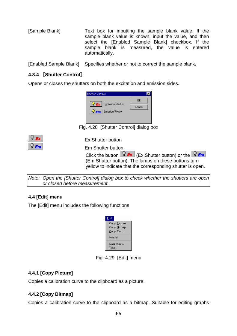
[Sample Blank] Text box for inputting the sample blank value. If the sample blank value is known, input the value, and then select the [Enabled Sample Blank] checkbox. If the sample blank is measured, the value is entered automatically.
[Enabled Sample Blank] Specifies whether or not to correct the sample blank.
4.3.4 [Shutter Control]
Opens or closes the shutters on both the excitation and emission sides.
Fig. 4.28 [Shutter Control] dialog box
Ex Shutter button Em Shutter button
Click the button (Ex Shutter button) or the (Em Shutter button). The lamps on these buttons turn yellow to indicate that the corresponding shutter is open.
Note: Open the [Shutter Control] dialog box to check whether the shutters are open
or closed before measurement.
4.4 [Edit] menu
The [Edit] menu includes the following functions
Fig. 4.29 [Edit] menu
4.4.1 [Copy Picture]
Copies a calibration curve to the clipboard as a picture.
4.4.2 [Copy Bitmap]
Copies a calibration curve to the clipboard as a bitmap. Suitable for editing graphs
55 55
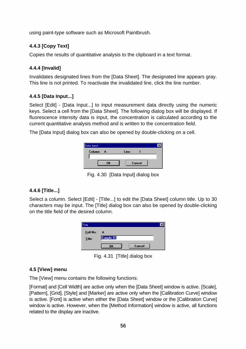
using paint-type software such as Microsoft Paintbrush.
4.4.3 [Copy Text]
Copies the results of quantitative analysis to the clipboard in a text format.
4.4.4 [Invalid]
Invalidates designated lines from the [Data Sheet]. The designated line appears gray. This line is not printed. To reactivate the invalidated line, click the line number.
4.4.5 [Data Input...]
Select [Edit] - [Data Input...] to input measurement data directly using the numeric keys. Select a cell from the [Data Sheet]. The following dialog box will be displayed. If fluorescence intensity data is input, the concentration is calculated according to the current quantitative analysis method and is written to the concentration field.
The [Data Input] dialog box can also be opened by double-clicking on a cell.
Fig. 4.30 [Data Input] dialog box
4.4.6 [Title...]
Select a column. Select [Edit] - [Title...] to edit the [Data Sheet] column title. Up to 30 characters may be input. The [Title] dialog box can also be opened by double-clicking on the title field of the desired column.
Fig. 4.31 [Title] dialog box
4.5 [View] menu
The [View] menu contains the following functions:
[Format] and [Cell Width] are active only when the [Data Sheet] window is active. [Scale], [Pattern], [Grid], [Style] and [Marker] are active only when the [Calibration Curve] window is active. [Font] is active when either the [Data Sheet] window or the [Calibration Curve] window is active. However, when the [Method Information] window is active, all functions related to the display are inactive.
56 56
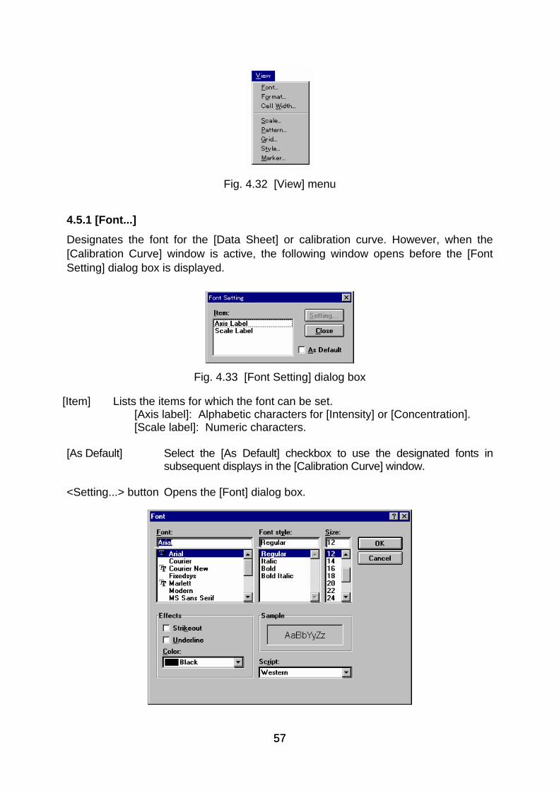
Fig. 4.32 [View] menu
4.5.1 [Font...]
Designates the font for the [Data Sheet] or calibration curve. However, when the [Calibration Curve] window is active, the following window opens before the [Font Setting] dialog box is displayed.
Fig. 4.33 [Font Setting] dialog box
[Item] Lists the items for which the font can be set. [Axis label]: Alphabetic characters for [Intensity] or [Concentration]. [Scale label]: Numeric characters. [As Default] Select the [As Default] checkbox to use the designated fonts in
subsequent displays in the [Calibration Curve] window. <Setting...> button Opens the [Font] dialog box.
57 57

Fig. 4.34 [Font] dialog box
[Font name] list The desired font can be selected from this list. [Style] list The desired font style can be selected from this list. [Size] list Lists possible font sizes. [Effects] Applies special character styles such as “strike out” or
“underlined”. [Color] list Allows font color to be selected. [Sample] Displays a sample of the selected font. [Script] Changes a script of the selected font.
4.5.2 [Format...]
Select the desired column. Select [View] - [Format...] to designate the number of decimal places that will be displayed on the [Data Sheet]. This setting can be different for each column. This function is active only when the [Data Sheet] window is active.
Fig. 4.35 [International Number Format] dialog box
4.5.3 [Cell Width...]
Select [View] - [Cell Width...] to set the cell width for each column of the [Data Sheet]. This function can only be selected when the [Data Sheet] window is active.
Fig. 4.36 [Cell Width] setting dialog box
[Cell Width] Text box for designating cell width. Input range is 4 to 32 characters.
[Default] The standard cell width is 12 characters.
4.5.4 [Scale...]
Select [View] - [Scale...] to set the scale of the vertical and horizontal axes of the calibration curve. Select the [Auto] checkbox to set the scale to the optimal value
58 58
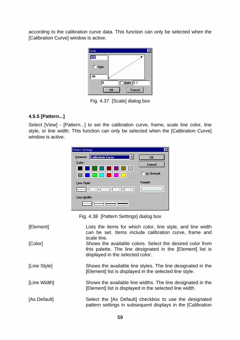
according to the calibration curve data. This function can only be selected when the [Calibration Curve] window is active.
Fig. 4.37 [Scale] dialog box
4.5.5 [Pattern...]
Select [View] - [Pattern...] to set the calibration curve, frame, scale line color, line style, or line width. This function can only be selected when the [Calibration Curve] window is active.
Fig. 4.38 [Pattern Settings] dialog box
[Element] Lists the items for which color, line style, and line width can be set. Items include calibration curve, frame and scale line.
[Color] Shows the available colors. Select the desired color from this palette. The line designated in the [Element] list is displayed in the selected color.
[Line Style] Shows the available line styles. The line designated in the
[Element] list is displayed in the selected line style. [Line Width] Shows the available line widths. The line designated in the
[Element] list is displayed in the selected line width. [As Default] Select the [As Default] checkbox to use the designated
pattern settings in subsequent displays in the [Calibration
59 59

Curve] window. [Sample] Displays a sample of the designated pattern.
4.5.6 [Grid...]
Select [View] - [Grid...] to designate whether or not to display the vertical and horizontal axes of the calibration curve. The function can only be selected when the [Calibration Curve] window is active.
Fig. 4.39 [Grid Lines] dialog box
[Main] Select the [Vertical Axis] and/or [Horizontal Axis] checkbox to display the scale line.
[Axial] Not used [As Default] Select the [As Default] checkbox to use the designated
grid lines in subsequent displays in the [Calibration Curve] window.
4.5.7 [Style...]
Select [View] - [Style...] to designate the scale interval and decimal places of the vertical and horizontal axes of the calibration curve. This function can only be selected when the [Calibration Curve] window is active.
Fig. 4.40 [Style Settings] dialog box
[Axis] Lists the axes for which the style can be designated.
60 60

Select [Concentration] or [Intensity]. [Scale Label] The scale interval and number of decimal places can be set. [Interval]: Allow the scale interval to be set to [Auto] or
[Manual]. [Auto]: The scale interval is set automatically. [Manual]: Text box for inputting main scale interval. [Decimal Point on Scale]: Sets the number of decimal places for the main scale. Default: #.### (three decimal places) Integer: Displays only the integer. #.#: Displays to one decimal place. #.##: Displays to two decimal places. [As Default] Select the [As Default] checkbox to use the designated
style settings for subsequent displays in the [Calibrate Curve] window.
4.5.8 [Marker...]
Select [View] - [Marker...] to designate the type, size, and color of the marker used to indicate specific data points on the calibration curve, and whether or not to fill the inside of the marker.
Fig. 4.41 [Marker Settings] dialog box
[Type] Lists the types of markers available. Marker types include circle, square, triangle, rhombus, or cross.
[Size] Sets the marker size. [Color] Shows the available colors. Select the desired color from
the palette. [Fill Inside] Select the [Fill Inside] checkbox to fill the inside of the
marker. [As Default] Select the [As Default] checkbox to use the designated
marker patterns in subsequent displays in the [Calibration Curve] window.
61 61

[Sample] Displays a sample of the designated marker.
4.6 [Window] menu
The display style of the [Data Sheet], [Calibration Curve], and [Method Information] windows can be designated from this menu.
Fig. 4.42 [Window] menu
4.6.1 [Cascade]
Select [Window] - [Cascade] to overlay the [Data Sheet], [Calibration Curve], and [Method Information] windows in the display as shown in the figure below.
Fig. 4.43 [Cascade] display
4.6.2 [Tile]
Select [Window] - [Tile] to display the [Data Sheet], [Calibration Curve], and [Method Information] windows side-by-side as shown in the figure below.
62 62

Fig. 4.44 [Tile] display
4.7 [Help] menu
Version information for the [Quantitative Analysis] program can be displayed from this menu.
Fig. 4.45 [Help] menu
4.7.1 [About...]
Select [Help] - [About...] to display version information for the [Quantitative Analysis] program.
Fig. 4.46 [About Quantitative Analysis] dialog box
63 63
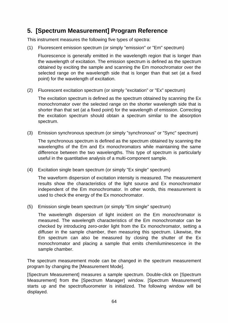
5. [Spectrum Measurement] Program Reference This instrument measures the following five types of spectra:
(1) Fluorescent emission spectrum (or simply "emission" or "Em" spectrum)
Fluorescence is generally emitted in the wavelength region that is longer than the wavelength of excitation. The emission spectrum is defined as the spectrum obtained by exciting the sample and scanning the Em monochromator over the selected range on the wavelength side that is longer than that set (at a fixed point) for the wavelength of excitation.
(2) Fluorescent excitation spectrum (or simply "excitation" or "Ex" spectrum)
The excitation spectrum is defined as the spectrum obtained by scanning the Ex monochromator over the selected range on the shorter wavelength side that is shorter than that set (at a fixed point) for the wavelength of emission. Correcting the excitation spectrum should obtain a spectrum similar to the absorption spectrum.
(3) Emission synchronous spectrum (or simply "synchronous" or "Sync" spectrum)
The synchronous spectrum is defined as the spectrum obtained by scanning the wavelengths of the Em and Ex monochromators while maintaining the same difference between the two wavelengths. This type of spectrum is particularly useful in the quantitative analysis of a multi-component sample.
(4) Excitation single beam spectrum (or simply "Ex single" spectrum)
The waveform dispersion of excitation intensity is measured. The measurement results show the characteristics of the light source and Ex monochromator independent of the Em monochromator. In other words, this measurement is used to check the energy of the Ex monochromator.
(5) Emission single beam spectrum (or simply "Em single" spectrum)
The wavelength dispersion of light incident on the Em monochromator is measured. The wavelength characteristics of the Em monochromator can be checked by introducing zero-order light from the Ex monochromator, setting a diffuser in the sample chamber, then measuring this spectrum. Likewise, the Em spectrum can also be measured by closing the shutter of the Ex monochromator and placing a sample that emits chemiluminescence in the sample chamber.
The spectrum measurement mode can be changed in the spectrum measurement program by changing the [Measurement Mode].
[Spectrum Measurement] measures a sample spectrum. Double-click on [Spectrum Measurement] from the [Spectrum Manager] window. [Spectrum Measurement] starts up and the spectrofluorometer is initialized. The following window will be displayed.
64
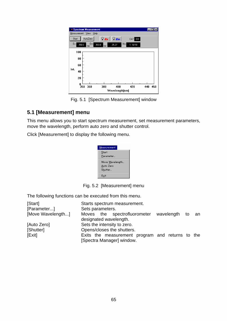
Fig. 5.1 [Spectrum Measurement] window
5.1 [Measurement] menu This menu allows you to start spectrum measurement, set measurement parameters, move the wavelength, perform auto zero and shutter control.
Click [Measurement] to display the following menu.
Fig. 5.2 [Measurement] menu
The following functions can be executed from this menu. [Start] Starts spectrum measurement. [Parameter...] Sets parameters. [Move Wavelength...] Moves the spectrofluorometer wavelength to an
designated wavelength. [Auto Zero] Sets the intensity to zero. [Shutter] Opens/closes the shutters. [Exit] Exits the measurement program and returns to the
[Spectra Manager] window.
65

5.1.1 [Start]
Starts spectrum measurement. The spectrum is displayed in real time during measurement.
Fig. 5.3 [Spectrum Measurement] window
When measurement has been completed, a new window is opened which displays a spectrum on the vertical axis set from the [Parameters] dialog box. At the same time, the standard analysis program starts.
Note1: After starting spectra analysis and performing the initial measurement, the [Spectrum View] showing the results of the most recent measurement will be displayed over the previously displayed [Spectrum View], which will no longer be visible. To keep the previous [Spectrum View], save or print it. To redisplay the hidden [Spectrum View], change the application.
Note2: If a measurement in progress is interrupted, the [Spectrum View] displays all
data obtained up to that point.
5.1.2 [Parameter...]
Set and save parameters. The parameter dialog box consists of 3 pages: [Parameters] dialog box, [Data File] dialog box and [Options] dialog box. Click the [Data File] tag while the [Parameters] dialog box is active to activate the [Data File] dialog box.
Parameters are set in the [Parameters] dialog box. Information such as the filename for automatically saving measurement data can be input in the [Data File] dialog box.
5.1.2.1 Parameter setting
Select [Measurement] - [Parameter...] to display the following dialog box.
66

Fig. 5.4 [Spectrum Measurement - Parameters] dialog box(Emission mode)
[Measurement Mode] The spectrum measurement mode can be changed in the spectrum measurement program by changing the [Measurement Mode].
This instrument measures the following five types of spectra:
Emission: Fluorescent emission spectrum Excitation: Fluorescent excitation spectrum Synchronous: Emission synchronous spectrum Ex Single: Excitation single beam spectrum Em Single: Emission single beam spectrum [Excitation Band Width] Spectral bandwidth of the Ex monochromator Selectable range : 1, 3, 5, 10, 20, L5, L10 nm [Emission Band Width] Spectral bandwidth of the Em monochromator Selectable range : 1, 3, 5, 10, 20, L5, L10 nm [Response] Response speed Selectable range : 0.01, 0.02, 0.05, 0.1, 0.2, 0.5, 1, 2, 4, 8 sec [Correction] Changes over the spectrum correcting function
valid/invalid. The check box can be displayed and set when the [Measurement Mode] is [Emission] or [Excitation]. Clicking the check box validates spectrum correction. Refer to ″Spectrum correction program operation manual″ for spectrum correction.
[Excitation Wavelength] Wavelength to excite sample Input range : 220 to 750 nm [Excitation Wavelength] will be displayed only in the
[Emission] and [Excitation] modes.
67

[Emission Wavelength] Em detecting wavelength(Em monochromator) Input range : 220 to 750 nm [Emission Wavelength] will be displayed only in the
[Excitation] mode. [Delta Wavelength] Difference between the wavelength of the Em
monochromator and that of the Ex monochromator Input range: -10 to 500 nm [Delta Wavelength] will be displayed only in the
[Synchronous] mode. [Start] Shorter wavelength end of the measurement wavelength
range Input range : 220 to 740 nm [End] Longer wavelength end of the Em spectrum measurement
wavelength range Input range : 230 to 750 nm Note: Normally, set the start/end wavelengths of the Em spectrum at wavelengths
longer the Ex wavelength and set the start/end wavelengths of the Ex spectrum at wavelengths shorter the Em wavelength
[Data Pitch] Designates data collecting wavelength interval and [Data Pitch].
Selectable range : 0.1, 0.2, 0.5, 1, 2, 5, 10 nm [Scanning Speed] Selectable range :
10, 20, 50, 100, 200, 500, 1000, 2000, 5000, 10000, 20000 nm/min.
[Sensitivity] Change the set value of the photomultiplier tube voltage. Selectable range: Low, Medium, High, or Manual Designates the Photomultiplier tube voltage ([PMT
voltage] text box) setting to Manual. [PMT Voltage] Designates the Photomultiplier tube voltage([PMT voltage]
text box), Setting to Manual. Input range : 0 to 1000 V [Sample No.] Designates which sample should be measured first.
Subsequent samples are measured in order from the first sample number, increasing in increments of one.
Input range: 1 to 999 [No. of Cycle] Designates the number of measurements for each sample.
If two or more measurements are designated, the [Cycle Time] field is displayed.
Input range: 1 to 9999 [Cycle Time] Designates the time between measurements in seconds. If
68

the designated time is shorter than the measurement time, the next measurement starts immediately.
Input range: 0 to 15000 sec. [Accumulate] If the [Accumulate] check box is selected, the
[Accumulation No.] text box will be displayed. Input the accumulation number. The spectrum is averaged using this accumulation number.
Input range: 1 to 9999 [Display] Sets the upper and lower limits of the vertical axis range
displayed on the CRT screen. If [Auto] is selected, the full-scale axis is set to approximately 1.2 times the maximum width of the displayed spectrum, based on the measurement result.
<OK> button Accepts the settings currently displayed in the dialog box
and closes the [Spectrum Measurement - Parameters] dialog box.
<Cancel> button Closes the [Spectrum Measurement - Parameters] dialog
box without changing the previous settings. Note: The possible combinations of [Response] and [Scanning speed] are limited to
those shown in Table 5.1. The possible combinations of [Scanning speed] and [Data pitch] are limited to those shown in Table 5.2.
Table 5.1 Possible combinations of [Response] and [Scanning speed] Scanning speed(nm/min) Response
(sec) 10 20 50 100 200 500 1000 2000 5000 10000 20000 0.01 0.02 0.05 0.1 0.2 0.5 1 2 4 8
○
○
○
○
○
○
○ ○ ○ ○
○
○
○
○
○
○
○ ○ ○ ○
○
○
○
○
○
○
○ ○ ○ ○
○ ○ ○ ○ ○ ○ ○ ○ ○ ○
○ ○ ○ ○ ○ ○ ○ ○ ○ ○
○ ○ ○ ○ ○ ○ ○ ○ × ×
○ ○ ○ ○ ○ ○ ○ × × ×
○ ○ ○ ○ ○ ○ × × × ×
○ ○ ○ ○ ○ × × × × ×
○ ○ ○ ○ × × × × × ×
○ ○ ○ × × × × × × ×
Table 5.2 Possible combinations of [Scanning speed] and [Data Pitch] Scanning speed(nm/min) Data pitch
(msec/data) 10 20 50 100 200 500 1000 2000 5000 10000 20000 0.1 0.2 0.5 1 2 5
10
○
○
○
○
○
○
○
○
○
○
○
○
○
○
○
○
○
○
○
○
○
○ ○ ○ ○ ○ ○ ○
○ ○ ○ ○ ○ ○ ○
○ ○ ○ ○ ○ ○ ○
× ○ ○ ○ ○ ○ ○
× × ○ ○ ○ ○ ○
× × × ○ ○ ○ ○
× × × × ○ ○ ○
× × × × × ○ ○
69
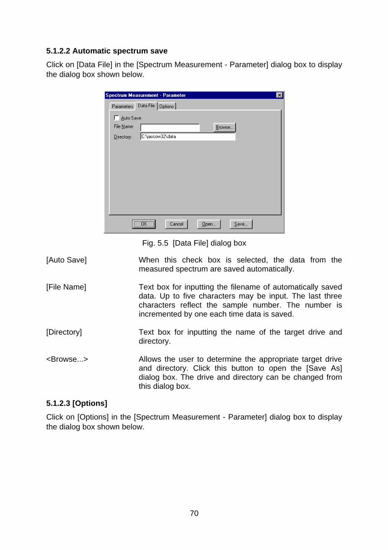
5.1.2.2 Automatic spectrum save
Click on [Data File] in the [Spectrum Measurement - Parameter] dialog box to display the dialog box shown below.
Fig. 5.5 [Data File] dialog box
[Auto Save] When this check box is selected, the data from the measured spectrum are saved automatically.
[File Name] Text box for inputting the filename of automatically saved
data. Up to five characters may be input. The last three characters reflect the sample number. The number is incremented by one each time data is saved.
[Directory] Text box for inputting the name of the target drive and
directory. <Browse...> Allows the user to determine the appropriate target drive
and directory. Click this button to open the [Save As] dialog box. The drive and directory can be changed from this dialog box.
5.1.2.3 [Options]
Click on [Options] in the [Spectrum Measurement - Parameter] dialog box to display the dialog box shown below.
70

Fig. 5.6 [Options] dialog box
[Sample Name], [Operator], [Copyright], [Comment] and [Accessory] can be designated by the user. Up to 62 characters can be input for each field. If the [Display ‘Comment Edit’ Dialog at Measurement] check box is selected, the [Comment edit] dialog box will be displayed during measurement.
5.1.2.4. Saving spectrum measurement parameters
Parameters can be saved to the parameter library on the disk.
Click <Save...> in the [Parameter] dialog box to open the dialog box shown below.
Fig. 5.7 [Parameters - Save] dialog box
[Parameter Name] Text box for inputting parameter name. A maximum of 32 characters may be input. Existing parameter names may be selected from the [Parameters List], in which case, the previous parameter settings will be overwritten.
<OK> Saves parameters.
71

<Cancel> Returns to the [Parameter] dialog box without saving the parameters.
<Contents...> Displays the parameters selected from the parameter list.
Use to confirm selections. <Delete> Deletes designated parameters from the parameters list.
5.1.2.5 Loading spectrum measurement parameters
Previously saved parameters in the parameter library can be selected. Click <Open...> in the [Spectrum Measurement - Parameter] dialog box. The following dialog box will be displayed.
Fig 5.8 [Parameters - Open] dialog box
[Parameters List] Lists available saved parameters. <OK> Loads selected parameter(s) from memory. <Cancel> Returns to the [Parameters] dialog box without loading
saved parameters. <Contents...> Displays selected parameters from the parameter list. Use
to confirm selections. <Delete> Deletes selected parameters from the parameter list.
5.1.3 [Goto Wavelength...]
Moves the spectrofluorometer wavelength to a designated wavelength. Select [Goto Wavelength] to display the dialog box shown below.
Fig. 5.9 [Goto Wavelength] dialog box
72
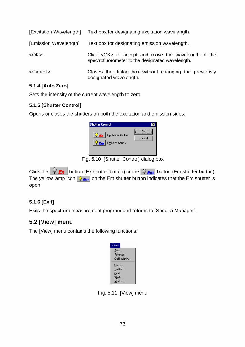
[Excitation Wavelength] Text box for designating excitation wavelength. [Emission Wavelength] Text box for designating emission wavelength. <OK>: Click <OK> to accept and move the wavelength of the
spectrofluorometer to the designated wavelength. <Cancel>: Closes the dialog box without changing the previously
designated wavelength.
5.1.4 [Auto Zero]
Sets the intensity of the current wavelength to zero.
5.1.5 [Shutter Control]
Opens or closes the shutters on both the excitation and emission sides.
Fig. 5.10 [Shutter Control] dialog box
Click the button (Ex shutter button) or the button (Em shutter button). The yellow lamp icon on the Em shutter button indicates that the Em shutter is open.
5.1.6 [Exit]
Exits the spectrum measurement program and returns to [Spectra Manager].
5.2 [View] menu The [View] menu contains the following functions:
Fig. 5.11 [View] menu
73

5.2.1 [Scale...]
Select [View] - [Scale...] to set the scale of the vertical and horizontal axes of the spectrum. Select the [Auto] checkbox to set the scale to the optimal value according to the spectrum data.
Fig. 5.12 [Scale] dialog box
5.2.2 [Pattern...]
Select [View] - [Pattern...] to set the spectrum, frame, scale line color, line style, or line width.
Fig. 5.13 [Pattern Settings] dialog box
[Element] Lists the items for which color, line style, and line width can be set. Items include spectrum, frame and scale line.
[Color] Shows the available colors. Select the desired color from this palette. The line designated in the [Element] list is displayed in the selected color.
[Line Style] Shows the available line styles. The line designated in the
[Element] list is displayed in the selected line style. [Line Width] Shows the available line widths. The line designated in the
[Element] list is displayed in the selected line width. [As Default] Select the [As Default] checkbox to use the designated
pattern settings in subsequent displays in the [Spectrum Measurement] window.
74

[Sample] Displays a sample of the designated pattern.
5.2.3 [Grid...]
Select [View] - [Grid...] to designate whether or not to display the vertical and horizontal axes of the spectrum.
Fig. 5.14 [Grid Lines] dialog box
[Main] Select the [Vertical Axis] and/or [Horizontal Axis] checkbox to display the scale line.
[Axial] Not used [As Default] Select the [As Default] checkbox to use the designated
grid lines in subsequent displays in the [Spectrum Measure] window.
5.2.4 [Style...]
Select [View] - [Style...] to designate the scale interval and decimal places of the vertical and horizontal axes of the calibration curve.
Fig. 5.15 [Style Settings] dialog box
[Axis] Lists the axes for which the style can be designated. [Scale Label] The scale interval and number of decimal places can be set. [Interval]: Allow the scale interval to be set to [Auto] or
[Manual].
75
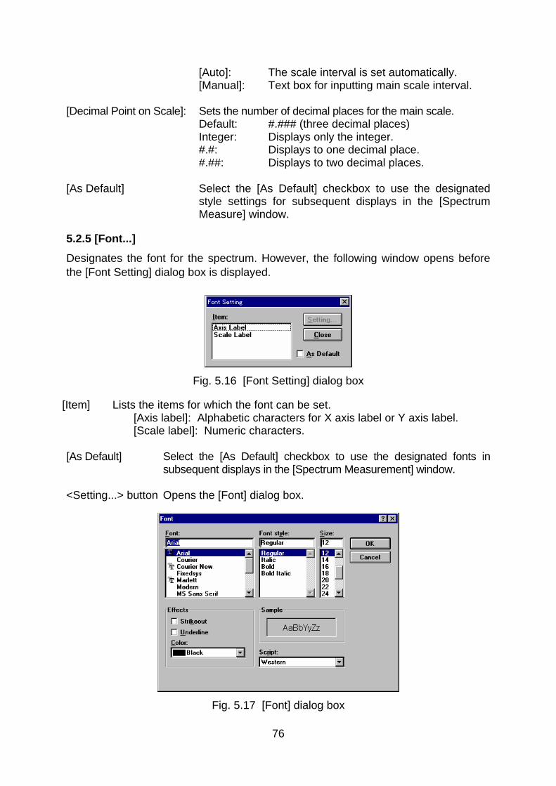
[Auto]: The scale interval is set automatically. [Manual]: Text box for inputting main scale interval. [Decimal Point on Scale]: Sets the number of decimal places for the main scale. Default: #.### (three decimal places) Integer: Displays only the integer. #.#: Displays to one decimal place. #.##: Displays to two decimal places. [As Default] Select the [As Default] checkbox to use the designated
style settings for subsequent displays in the [Spectrum Measure] window.
5.2.5 [Font...]
Designates the font for the spectrum. However, the following window opens before the [Font Setting] dialog box is displayed.
Fig. 5.16 [Font Setting] dialog box
[Item] Lists the items for which the font can be set. [Axis label]: Alphabetic characters for X axis label or Y axis label. [Scale label]: Numeric characters. [As Default] Select the [As Default] checkbox to use the designated fonts in
subsequent displays in the [Spectrum Measurement] window. <Setting...> button Opens the [Font] dialog box.
Fig. 5.17 [Font] dialog box
76

[Font name] list The desired font can be selected from this list. [Style] list The desired font style can be selected from this list. [Size] list Lists possible font sizes. [Effects] Applies special character styles such as “strike out” or
“underlined”. [Color] list Allows font color to be selected. [Sample] Displays a sample of the selected font. [Script] Changes a script of the selected font.
5.3 [Help] menu Displays information such as program version.
Fig. 5.18 [About FP Driver] dialog box
77

6 [Time Course Measurement] Program Reference Measures changes in a sample over time at a designated wavelength.
Double-click [Time Course Measurement] in the [Spectra Manager] window. The [Time Course Measurement] program will start, and the window shown below will open.
Fig. 6.1 [Time Course Measurement] window
6.1 [Measurement] menu This menu allows you to start time course measurement, set measurement parameters, move the wavelength, execute auto zero and perform shutter control.
Select [Measurement] to display the menu shown below.
Fig. 6.2 [Measurement] menu
78
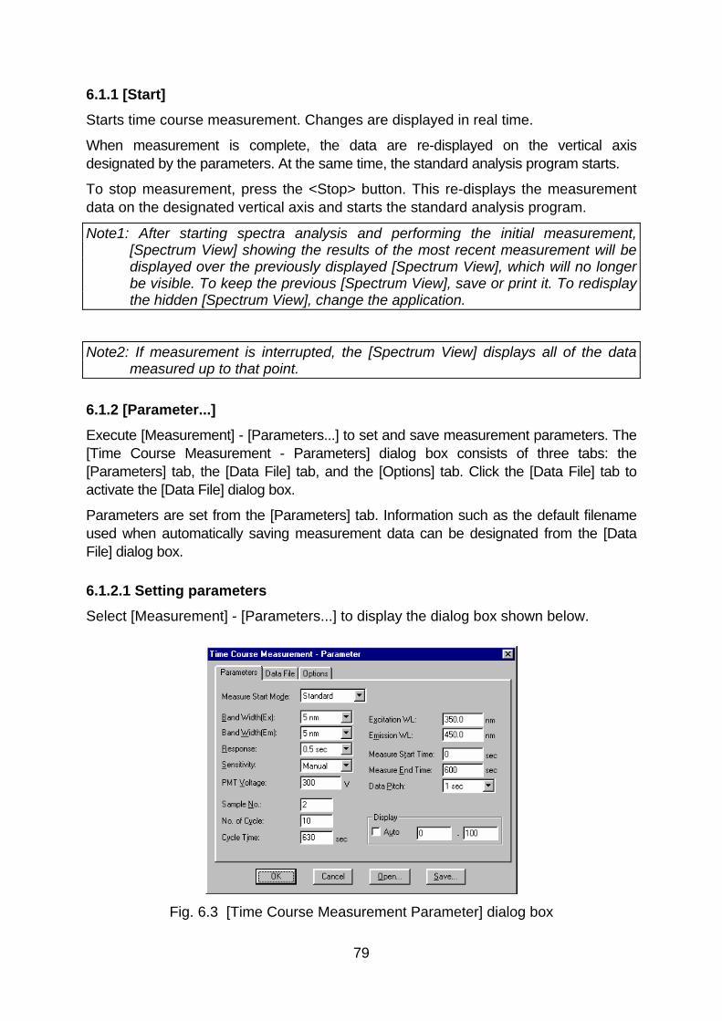
6.1.1 [Start]
Starts time course measurement. Changes are displayed in real time.
When measurement is complete, the data are re-displayed on the vertical axis designated by the parameters. At the same time, the standard analysis program starts.
To stop measurement, press the <Stop> button. This re-displays the measurement data on the designated vertical axis and starts the standard analysis program.
Note1: After starting spectra analysis and performing the initial measurement, [Spectrum View] showing the results of the most recent measurement will be displayed over the previously displayed [Spectrum View], which will no longer be visible. To keep the previous [Spectrum View], save or print it. To redisplay the hidden [Spectrum View], change the application.
Note2: If measurement is interrupted, the [Spectrum View] displays all of the data
measured up to that point.
6.1.2 [Parameter...]
Execute [Measurement] - [Parameters...] to set and save measurement parameters. The [Time Course Measurement - Parameters] dialog box consists of three tabs: the [Parameters] tab, the [Data File] tab, and the [Options] tab. Click the [Data File] tab to activate the [Data File] dialog box.
Parameters are set from the [Parameters] tab. Information such as the default filename used when automatically saving measurement data can be designated from the [Data File] dialog box.
6.1.2.1 Setting parameters
Select [Measurement] - [Parameters...] to display the dialog box shown below.
Fig. 6.3 [Time Course Measurement Parameter] dialog box
79

[Measure Start Mode] Sets the Ex shutter in measurement (when the <Start> button is pressed).
Standard Starts measurement in the currently set status. Shutter open Starts measurement after opening the Ex shutter. Shutter close Starts measurement after closing the Ex shutter. Note: Set the Em shutter properly by manual operation because it is not controlled.
[Trigger start] Starts measurement when the [Measurement Start] switch
(see Fig. 3.10) is pressed after the <Start> button is pressed. At this time, the [Power lamp] (see Fig. 3.10) blinks red. Clicking the check box validates this function.
[Excitation Wavelength] Wavelength used to excite sample Input range : 220 to 750 nm [Emission Wavelength] Em detecting wavelength(Em monochromator) Input range : 220 to 750 nm [Excitation Band Width] Spectral bandwidth of the Ex monochromator Selectable range : 1, 3, 5, 10, 20, L5, L20 nm [Emission Band Width] Spectral bandwidth of the Em monochromator Selectable range : 1, 3, 5, 10, 20, L5, L20 nm [Response] Response speed Selectable range : 0.01, 0.02, 0.05, 0.1, 0.2, 0.5, 1, 2, 4, 8 sec [Sensitivity] Used to change the set value of the photomultiplier tube
voltage. Selectable range: Low, Medium, High, Manual Designates the Photomultiplier tube voltage([PMT voltage]
text box), Setting to Manual. [PMT Voltage] Designates the Photomultiplier tube voltage([PMT voltage]
text box), Setting to Manual. Input range : 0 to 1000 V [Measure Start Time] Input range : -100 to 100 sec [Measure End Time] Input range : 1 to 12000 sec [Data Pitch] Used to designate the data collecting wavelength interval. Selectable range : 0.01, 0.02, 0.05, 0.1, 0.2, 0.5, 1, 2, 5, 10 sec [Sample No.] Used to designate the sample to be measured first.
Subsequent samples are measured in order from the first sample number, increasing in increments of one.
80

Input range : 1 to 999 [No. of Cycle] Designates the number of measurements for each sample.
If two or more measurements are designated, the [Cycle Time] field is displayed.
Input range: 1 to 9999 [Cycle Time] Designates the time between measurements in seconds. If
the designated time is shorter than the measurement time, the next measurement starts immediately.
Input range: 0 to 15000 sec. [Display] Used to set the higher and lower limits of the vertical axis
range. If [Auto] is selected, the full-scale axis is set to approximately 1.2 times the maximum width of the displayed data, based on the measurement result.
<OK> Confirms the current parameter settings and exits the
dialog box. Click this button to transfer the set parameters to the spectrofluorometer.
<Cancel> Exits the dialog box without changing the settings.
6.1.2.2 Automatic time course data save
Click [Data File] in the [Time Course Measurement Parameter] dialog box to display the dialog box shown below. For details, refer to Section 5.1.2.2.
Fig. 6.4 [Data File] dialog box
6.1.2.3 [Options]
Click on [Options] in the [Time Course Measurement Parameter] dialog box to display the dialog box shown below. For details, refer to Section 5.1.2.3.
81

Fig. 6.5 [Options] dialog box
6.1.2.4 Saving time course parameters
Saves the parameters in the parameter library on the disk. Click <Save...> in the [Time Course Measurement - Parameters] dialog box to open the dialog box shown below. For details, refer to Section 5.1.2.4.
Fig. 6.6 [Parameters - Save] dialog box
6.1.2.5 Loading spectrum measurement parameters
Previously saved parameters in the parameter library can be selected. Click <Open...> in the [Time Course Measurement - Parameters] dialog box to open the dialog box shown below. For details, refer to Section 5.1.2.5.
82

Fig. 6.7 [Parameters - Open] dialog box
6.1.3 [Goto Wavelength...]
Used to move the spectrofluorometer wavelength to a designated wavelength. For details, refer to Section 5.1.3.
6.1.4 [Auto Zero]
Used to set the intensity at the current wavelength to zero.
6.1.5 [Shutter Control]
Used to open or close the shutters on both the excitation and emission sides.
Note: See Section 5.1.5, for details.
6.1.6 [Exit]
Exits the time course measurement program and returns to [Spectra Manager].
6.2 [View] menu The [View] menu contains the following functions:
Fig. 6.8 [View] menu
Note: See Section 5.2, for details.
6.3 [Help] menu Displays information such as program version. See Section 5.3, for details
83

7. [Fixed Wavelength Measurement] [Fixed Wavelength Measurement] measures sample fluorescence intensity at a fixed wavelength. This program enables multiple wavelength measurements. Up to four wavelength settings (for Ex or Em) are possible. When multiple wavelengths are set on the Ex side, the Em side must be set to one fixed wavelength. Likewise, when multiple wavelengths are set on the Em side, the Ex side must be set to one fixed wavelength.
When the [Fixed Wavelength Measurement] program is started, the window shown below will be displayed.
Fig. 7.1 [Fixed Wavelength Measurement] window
7.1 [Measurement] menu This menu allows you to start fixed wavelength measurement, set measurement parameters, move the wavelength, execute auto zero and perform shutter control.
Select [Measurement] to display the menu shown below.
Fig. 7.2 [Measurement] menu
7.1.1 [Start]
Starts fixed wavelength measurement. To suspend measurement, click <Stop>.
7.1.2 [Parameter...]
Used to set parameters and save parameters to the disk.
84

7.1.2.1 Setting fixed wavelength parameters
Select [Measurement] - [Parameters...] to display the dialog box shown below.
Fig. 7.3 [Fixed Wavelength Measurement] dialog box
[Excitation Band Width] Spectral bandwidth of the Ex monochromator Selectable range : 1, 3, 5, 10, 20, L5, L10 nm [Emission Band Width] Spectral bandwidth of the Em monochromator Selectable range : 1, 3, 5, 10, 20, L5, L10 nm [Response] Response speed Selectable range : 0.01, 0.02, 0.05, 0.1, 0.2, 0.5, 1, 2, 4, 8 sec [Sensitivity] Used to change the set value of the photomultiplier tube
voltage. Selectable range: Low, Medium, High, Manual Used to change the Photomultiplier tube voltage ([PMT
voltage] text box) setting to Manual. [PMT Voltage] Used to change the Photomultiplier tube voltage ([PMT
voltage] text box) setting to Manual. Input range: 0 to 1000 V [Emission] Used to designate up to four Em wavelength settings for
one fixed Ex wavelength. Input range: 220 to 750 nm [Excitation] Used to designate up to four Ex wavelength settings for
one fixed Em wavelength. Input range: 220 to 750 nm [Random] Used to designate up to four combined Em-Ex wavelength
settings that are to be selected. [1] ~ [4] Option buttons for selecting the number of wavelengths. [Wavelength of excitation] Text box for entering Ex wavelength settings. [Wavelength of emission] Text book for entering Em wavelength settings.
85
The operation procedure is as follows:
1) Select the measurement method (Emission, Excitation, or Random). 2) Select the number of wavelengths from [1] ~ [4]. 3) Enter the Ex and Em wavelength settings in each text box.
Note: Set the number of wavelengths to [1] for single wavelength measurement (i.e.,
one wavelength for excitation, one wavelength for emission)
[Sample No.] Used to designate which sample should be measured first. Subsequent samples are measured in order from the first sample number, increasing in increments of one.
Input range: 1 to 999 [No. of Cycles] Used to designate the number of measurements for each
sample. If two or more measurements are designated, the [Cycle Time] field is displayed. If the sample is measured by setting multiple cycles, measurement values for each of the cycles, as well as the average value, are displayed.
Input range: 1 to 9999. [Cycle Time] Used to designate the time (in seconds) between
measurements. If the designated time is shorter than the measurement time, the next measurement will start immediately after completion of the previous measurement.
Input range: 0 to 15000 sec. <OK> Confirms the current parameter settings and exits the
dialog box. Click this button to transfer the set parameters to the spectrofluorometer.
<Cancel> Exits the dialog box without changing the settings.
7.1.2.2 Saving fixed wavelength parameters
Parameters can be saved to the parameter library on the disk.
For details, refer to Section 5.1.2.4.
7.1.2.3 Loading fixed wavelength parameters
Previously saved parameters in the parameter library can be selected.
For details, refer to Section 5.1.2.5.
7.1.3 [Goto Wavelength...]
Used to move the spectrofluorometer wavelength to a designated wavelength. For details, refer to Section 5.1.3.
7.1.4 [Auto Zero]
Used to set intensity at the current wavelength to zero.
86

7.1.5 [Shutter Control]
Used to open or close the shutters on both the excitation and emission sides. For details, refer to Section 5.1.5.
7.1.6 [Exit]
Exits the [Fixed Wavelength Measurement] program and returns to [Spectra Manager].
7.2 [Data] Deletes, saves and prints the data displayed in the window. The [Data] menu is shown below.
Fig. 7.4 [Data] menu
7.2.1 [New]
Deletes the displayed data and creates a new data file. Be careful, any data not saved on the disk will be lost.
7.2.2 [Save As...]
Saves data under a designated name. For details, refer to Section 4.1.4.
7.2.3 [Print...]
Prints the data. For details, refer to Section 4.1.7.
7.2.4 [Print Setup...]
Used to designate the target printer and the printing conditions. For details, refer to Section 4.1.6.
7.3 [Help] menu Displays information such as program version. For details, refer to Section 4.7.
87

8. [FP Intensity Monitor] The [FP Intensity Monitor] displays the fluorescence intensity of the specified wavelength. This monitor allows the user to conveniently check the fluorescence intensity at a glance.
When the [FP Intensity Monitor] program is started, the following window will be displayed:
Fig. 8.1 [FP Intensity Monitor] window
<Hold>/<Start> button Click this button to accept a measurement value. When
the fluorescence intensity is fixed in position, this button changes to <Start>. Click this button a second time to return to original status. This function is useful for obtaining data when the fluorescence intensity is unsteady.
<Auto Zero> button Sets the fluorescence intensity at the current wavelength
to zero. <Goto WL...> button Used to move the fluorescence intensity to a designated
wavelength. For details, refer to Section 5.1.3. <Settings...> button Used to set the parameters in the [Parameters] dialog box.
Fig. 8.2 [Parameters] dialog box
[Excitation Band Width] Spectral bandwidth of the Ex monochromator Selectable range: 1, 3, 5, 10, 20, L5, L10 nm
88

[Emission Band Width] Spectral bandwidth of the Em monochromator Selectable range: 1, 3, 5, 10, 20, L5, L10 nm [Response] Response speed
Selectable range: 0.01, 0.02, 0.05, 0.1, 0.2, 0.5, 1, 2, 4, 8 sec
[Sensitivity] Used to change the set value of the photomultiplier tube
voltage. Selectable range: Low, Medium, High, Manual Used to change the Photomultiplier tube voltage ([PMT
voltage] text box) setting to Manual. [PMT Voltage] Used to change the Photomultiplier tube voltage ([PMT
voltage] text box) setting to Manual. Input range: 0 to 1000 V <About…> button Displays the software version number.
Fig. 8.3 [About] dialog box
89
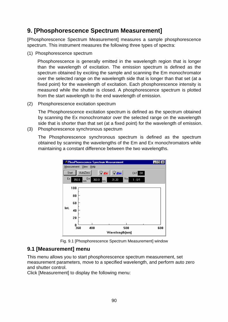
9. [Phosphorescence Spectrum Measurement] [Phosphorescence Spectrum Measurement] measures a sample phosphorescence spectrum. This instrument measures the following three types of spectra:
(1) Phosphorescence spectrum
Phosphorescence is generally emitted in the wavelength region that is longer than the wavelength of excitation. The emission spectrum is defined as the spectrum obtained by exciting the sample and scanning the Em monochromator over the selected range on the wavelength side that is longer than that set (at a fixed point) for the wavelength of excitation. Each phosphorescence intensity is measured while the shutter is closed. A phosphorescence spectrum is plotted from the start wavelength to the end wavelength of emission.
(2) Phosphorescence excitation spectrum
The Phosphorescence excitation spectrum is defined as the spectrum obtained by scanning the Ex monochromator over the selected range on the wavelength side that is shorter than that set (at a fixed point) for the wavelength of emission.
(3) Phosphorescence synchronous spectrum
The Phosphorescence synchronous spectrum is defined as the spectrum obtained by scanning the wavelengths of the Em and Ex monochromators while maintaining a constant difference between the two wavelengths.
Fig. 9.1 [Phosphorescence Spectrum Measurement] window
9.1 [Measurement] menu This menu allows you to start phosphorescence spectrum measurement, set measurement parameters, move to a specified wavelength, and perform auto zero and shutter control. Click [Measurement] to display the following menu:
90

Fig. 9.2 [Measurement] menu
The following functions can be performed from this menu: [Start] Starts spectrum measurement. [Parameter...] Used to set parameters. [Goto Wavelength...] Used to move the spectrofluorometer wavelength to a
designated wavelength. [Auto Zero] Sets the intensity to 0. [Shutter] Used to open/close the shutters. [Exit] Exits the measurement program and returns to the
[Spectra Manager] window.
9.1.1 [Start] Starts phosphorescence spectrum measurement. The spectrum is displayed in real time during measurement. When measurement has been completed, a new window opens displaying a spectrum on the vertical axis set from the [Parameters] dialog box. At the same time, the standard analysis program is started. Note1: After starting spectra analysis and performing the initial measurement,
[Spectrum View] showing the results of the most recent measurement will be displayed over the previously displayed [Spectrum View], which will no longer be visible. To keep the previous [Spectrum View], save or print it. To redisplay the hidden [Spectrum View], change the application
Note2: If measurement is interrupted, the [Spectrum View] will display all data
measured up to that point.
9.1.2 [Parameter...]
Used to set and save parameters. The [Parameters…] dialog box consists of three tabs: the [Parameters] tab, the [Data File] tab, and the [Options] tab. Click the [Data File] tab while the [Parameters…] dialog box is active to activate the [Data File] dialog box.
Parameters are set from the [Parameters] tab. Information such as the default filename used when automatically saving measurement data can be designated from the [Data File] dialog box.
91
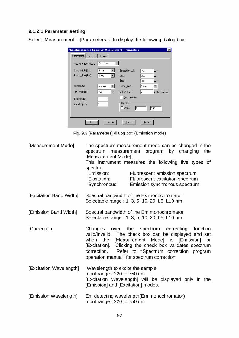
9.1.2.1 Parameter setting
Select [Measurement] - [Parameters...] to display the following dialog box:
Fig. 9.3 [Parameters] dialog box (Emission mode)
[Measurement Mode] The spectrum measurement mode can be changed in the
spectrum measurement program by changing the [Measurement Mode].
This instrument measures the following five types of spectra:
Emission: Fluorescent emission spectrum Excitation: Fluorescent excitation spectrum Synchronous: Emission synchronous spectrum [Excitation Band Width] Spectral bandwidth of the Ex monochromator Selectable range : 1, 3, 5, 10, 20, L5, L10 nm [Emission Band Width] Spectral bandwidth of the Em monochromator Selectable range : 1, 3, 5, 10, 20, L5, L10 nm [Correction] Changes over the spectrum correcting function
valid/invalid. The check box can be displayed and set when the [Measurement Mode] is [Emission] or [Excitation]. Clicking the check box validates spectrum correction. Refer to ″Spectrum correction program operation manual″ for spectrum correction.
[Excitation Wavelength] Wavelength to excite the sample Input range : 220 to 750 nm [Excitation Wavelength] will be displayed only in the
[Emission] and [Excitation] modes. [Emission Wavelength] Em detecting wavelength(Em monochromator) Input range : 220 to 750 nm
92

[Emission Wavelength] will be displayed only in the [Excitation] mode.
[Delta Wavelength] Difference between the wavelength of the Em monochromator and that of the Ex monochromator
Input range: -10 to 500 nm [Delta Wavelength] will be displayed only in the
[Synchronous] mode. [Start] Shorter wavelength end of the measurement wavelength
range Input range : 220 to 740 nm [End] Longer wavelength end of the Em spectrum measurement
wavelength range Input range : 230 to 750 nm Note: Normally, the start/end wavelengths of the Em spectrum should be set at
wavelengths that are longer than the Ex wavelength and the start/end wavelengths of the Ex spectrum should be set at wavelengths that are shorter than the Em wavelength.
[Data Pitch] Designates data collecting wavelength interval and [Data Pitch].
Selectable range: 0.1, 0.2, 0.5, 1, 2, 5, 10 nm [Delay Time (10 msec)] Input range: 0 to response10 [Sensitivity] Used to change the set value of the photomultiplier tube
voltage. Selectable range: Low, Medium, High, Manual Used to designate the Photomultiplier tube voltage ([PMT
voltage] text box) setting to Manual. [PMT Voltage] Used to designate the Photomultiplier tube voltage ([PMT
voltage] text box) setting to Manual. Input range : 0 to 1000 V [Sample No.] Used to designate which sample should be measured first.
Subsequent samples are measured in order from the first sample number, increasing in increments of one.
Input range : 1 to 999 [No. of Cycle] Used to designate the number of measurements for each
sample. If two or more measurements are designated, the [Cycle Time] field is displayed.
Input range : 1 to 9999 [Cycle Time] Used to designate the time (in seconds) between
measurements. If the designated time is shorter than the measurement time, the next measurement will start immediately following the previous measurement.
Input range: 0 to 15000 sec
93

[Accumulate] If the [Accumulate] check box is selected, the [Accumulation No.] text box will be displayed. Input the number of accumulations. The spectrum is averaged using this accumulation number.
Input range: 1 to 9999 [Display] Used to set the higher and lower limits of the vertical axis
range. If [Auto] is selected, the full-scale axis is set to approximately 1.2 times the maximum width of the displayed spectrum, based on the measurement result.
<OK> Confirms the current parameter settings and exits the
dialog box. Click this button to transfer the set parameters to the spectrofluorometer.
<Cancel> Exits the dialog box without changing the settings.
9.1.2.2 Automatic phosphorescence spectrum save
Click [Data File] in the [Phosphorescence Spectrum Measurement - Parameters] dialog box to display the dialog box shown below. For details, refer to Section 5.1.2.2.
Fig. 9.4 [Options] dialog box
9.1.2.3 [Options]
Click on [Options] in the [Phosphorescence Spectrum Measurement - Parameter] dialog box to display the dialog box shown below. For details, refer to Section 5.1.2.3.
94

Fig. 9.5 [Options] dialog box
9.1.2.4 Saving phosphorescence spectrum measurement parameters
Parameters are saved in the parameter library on the disk. Click <Save...> in the [Phosphorescence Spectrum Measurement - Parameters] dialog box to open the dialog box shown below. For details, refer to Section 5.1.2.4.
Fig. 9.6 [Parameters - Save] dialog box
9.1.2.5 Loading phosphorescence spectrum measurement parameters
Parameters previously saved in the parameter library can be selected. Click <Open...> in the [Phosphorescence Spectrum Measurement - Parameters] dialog box to open the dialog box shown below. For details, refer to Section 5.1.2.5.
Fig. 9.7 [Parameters - Open] dialog box
95
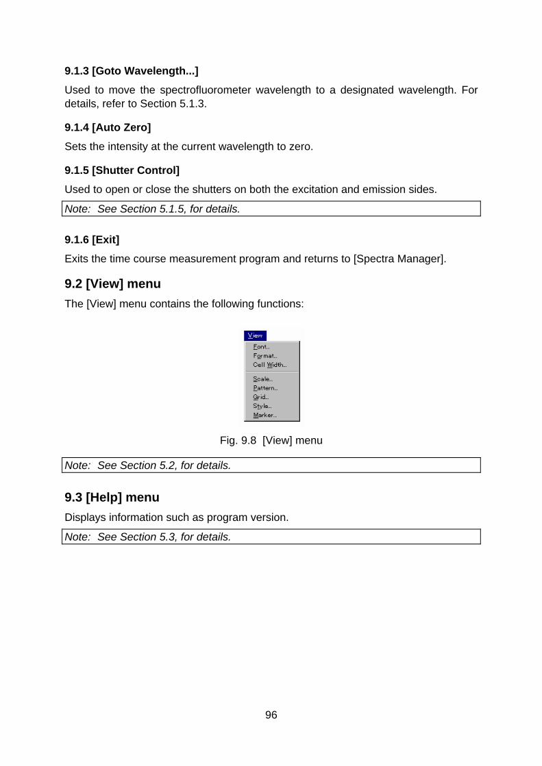
9.1.3 [Goto Wavelength...]
Used to move the spectrofluorometer wavelength to a designated wavelength. For details, refer to Section 5.1.3.
9.1.4 [Auto Zero]
Sets the intensity at the current wavelength to zero.
9.1.5 [Shutter Control]
Used to open or close the shutters on both the excitation and emission sides.
Note: See Section 5.1.5, for details.
9.1.6 [Exit]
Exits the time course measurement program and returns to [Spectra Manager].
9.2 [View] menu The [View] menu contains the following functions:
Fig. 9.8 [View] menu
Note: See Section 5.2, for details.
9.3 [Help] menu Displays information such as program version.
Note: See Section 5.3, for details.
96

10. [Phosphorescence Lifetime Measurement] Used to measure changes in a sample over time while the shutter is closed. Double-click [Phosphorescence Lifetime Measurement] in the [Spectra Manager] window. The [Phosphorescence Lifetime Measurement] programs will start, and the window shown below will be opened.
Fig. 10.1 [Phosphorescence Lifetime Measurement] window
10.1 [Measurement] menu This menu allows you to start phosphorescence spectrum measurement, set measurement parameters, move to a specified wavelength, and perform auto zero and shutter control. Click [Measurement] to display the following menu:
Fig. 10.2 [Measurement] menu
10.1.1 [Start] Starts phosphorescence lifetime measurement. The spectrum is displayed in real time during measurement. When measurement has been completed, a new window opens, displaying a spectrum on the vertical axis that is set in the [Parameters] dialog box. At the same time, the standard analysis program is started.
10.1.2 [Parameter...]
Used to set and save parameters. The parameter dialog box consists of three tabs: the [Parameters] tab, the [Data File] tab, and the [Options] tab. Click the [Data File] tab while the [Parameters] dialog box is active to activate the [Data File] dialog box.
97

Parameters are set from the [Parameters] tab. Information such as the default filename used when automatically saving measurement data can be designated from the [Data File] dialog box.
10.1.2.1 Parameter setting
Select [Measurement] - [Parameters...] to display the following dialog box.
Fig. 10.3 [Phosphorescence Lifetime Measurement - Parameters] dialog box
[Excitation Wavelength] Wavelength used to excite sample Input range : 220 to 750 nm [Emission Wavelength] Em detecting wavelength(Em monochromator) Input range : 220 to 750 nm [Excitation Band Width] Spectral bandwidth of the Ex monochromator Selectable range : 1, 3, 5, 10, 20, L5, L10 nm [Emission Band Width] Spectral bandwidth of the Em monochromator Selectable range : 1, 3, 5, 10, 20, L5, L10 nm [Response] Response speed Selectable range : 0.01, 0.02, 0.05, 0.1, 0.2, 0.5, 1, 2, 4, 8 sec [Sensitivity] Used to change the set value of the photomultiplier tube
voltage. Selectable range: Low, Medium, High, Manual Used to designate the Photomultiplier tube voltage ([PMT
voltage] text box) setting to Manual. [PMT Voltage] Used to designate the Photomultiplier tube voltage ([PMT
voltage] text box) setting to Manual. Input range: 0 to 1000 V
98

[Delay Time] (1/10 msec) Input range: 0 to 1000 msec [Measure Time] Input range : 1 to 10000 msec [Data Pitch] Used to designate data collecting wavelength interval. Selectable range : 0.1, 0.2, 0.5, 1, 2, 5, 10 msec [Sample No.] Used to designate which sample should be measured first.
Subsequent samples are measured in order from the first sample number, increasing in increments of one.
Input range: 1 to 999 [Display] Sets the higher and lower limits of the vertical axis range.
If [Auto] is selected, the full-scale axis is set to approximately 1.2 times the maximum width of the displayed data, based on the measurement result.
<OK> Confirms the current parameter settings and exits the
dialog box. Click this button to transfer the set parameters to the spectrofluorometer.
<Cancel> Exits the dialog box without changing the settings.
10.1.2.2 Automatic phosphorescence lifetime data save
Click [Data File] in the [Phosphorescence Lifetime Measurement – Parameters] dialog box to display the dialog box shown below. For details, refer to Section 5.1.2.2.
Fig. 10.4 [Options] dialog box
10.1.2.3 [Options]
Click on [Options] in the [Phosphorescence Lifetime Measurement - Parameter] dialog box to display the dialog box shown below. For details, refer to Section 5.1.2.3.
99
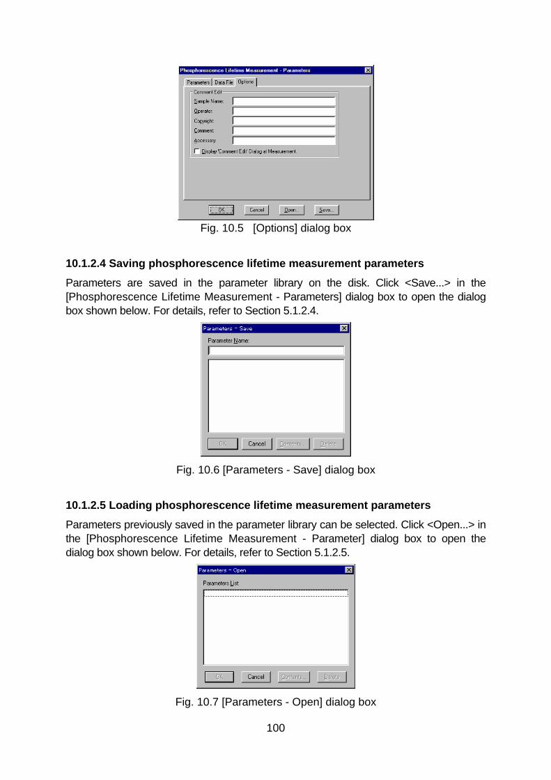
Fig. 10.5 [Options] dialog box
10.1.2.4 Saving phosphorescence lifetime measurement parameters
Parameters are saved in the parameter library on the disk. Click <Save...> in the [Phosphorescence Lifetime Measurement - Parameters] dialog box to open the dialog box shown below. For details, refer to Section 5.1.2.4.
Fig. 10.6 [Parameters - Save] dialog box
10.1.2.5 Loading phosphorescence lifetime measurement parameters
Parameters previously saved in the parameter library can be selected. Click <Open...> in the [Phosphorescence Lifetime Measurement - Parameter] dialog box to open the dialog box shown below. For details, refer to Section 5.1.2.5.
Fig. 10.7 [Parameters - Open] dialog box
100
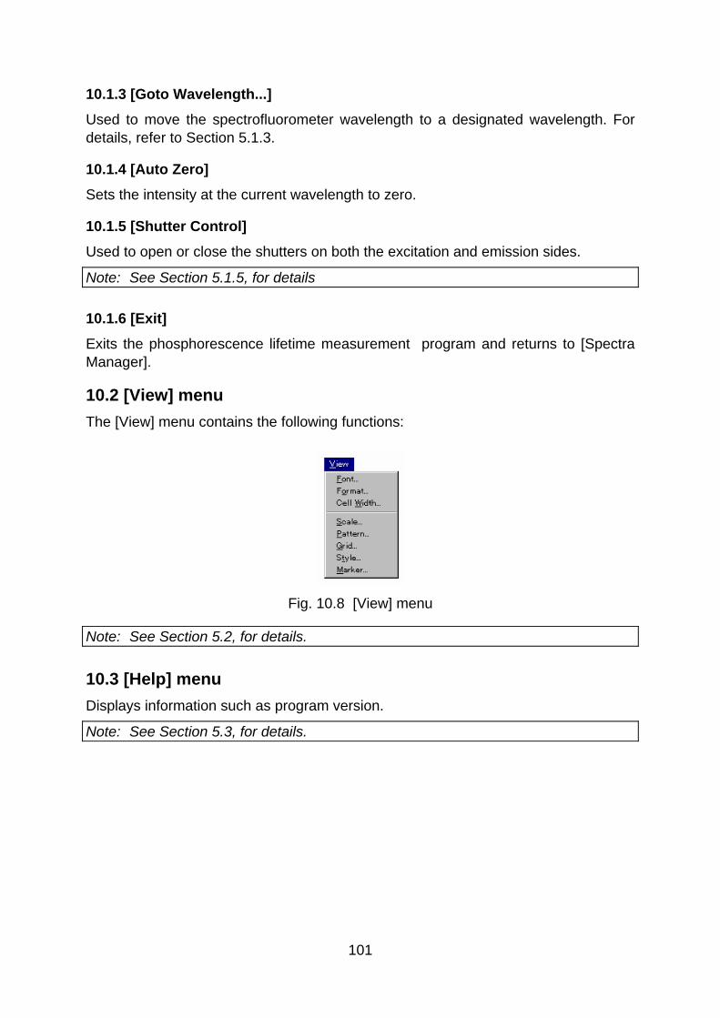
10.1.3 [Goto Wavelength...]
Used to move the spectrofluorometer wavelength to a designated wavelength. For details, refer to Section 5.1.3.
10.1.4 [Auto Zero]
Sets the intensity at the current wavelength to zero.
10.1.5 [Shutter Control]
Used to open or close the shutters on both the excitation and emission sides.
Note: See Section 5.1.5, for details
10.1.6 [Exit]
Exits the phosphorescence lifetime measurement program and returns to [Spectra Manager].
10.2 [View] menu The [View] menu contains the following functions:
Fig. 10.8 [View] menu
Note: See Section 5.2, for details.
10.3 [Help] menu Displays information such as program version.
Note: See Section 5.3, for details.
101

11. [Environment] System hardware settings, self-diagnostics, and optional accessory settings can be selected from this menu.
Start the Environment program to display the [Environment] dialog box. Select the desired item.
Fig. 11.1 [Environment] dialog box
[Items] List of setting items Hardware Setting: Xenon lamp off, Mercury lamp on/off,
lamp hours display Diagnostics: Allows operator to recognize any
instrument-related problems immediately.
Accessory Settings: Setting parameters for optional accessories.
11.1 [Hardware Setting] menu Xenon lamp off, Mercury lamp on/off, and the lamp hours display can be selected from this menu.
Fig. 11.2 [Hardware Setting] dialog box
[Xenon Lamp] [Lamp] check box Turns off the Xenon lamp. To turn the lamp back on, the
main unit power switch must be turned off, and then turned on again.
102

[Lamp Hours] text box Shows the hours that the Xenon lamp has been used. Enter zero in the text box when the lamp is replaced.
[Mercury Lamp] [Lamp] check box Turns on/off the Mercury lamp. [Lamp Hours] text box Shows the hours that the Xenon lamp has been used.
Enter zero in the text box when the lamp is replaced.
11.2 [Hardware Diagnostics] menu This menu allows the operator to recognize any instrument-related problems immediately.
Fig. 11.3 [Diagnosis] dialog box
[Ex grating drive] Checks whether the Ex monochromator is operating normally.
[Em grating drive] Checks whether the Em monochromator is operating
normally. [Ex slits drive] Checks whether the Ex slits drive is operating normally. [Em slits drive] Checks whether the Em slits drive is operating normally. [Ex PMT voltage] Checks whether the Ex PMT voltage is normal. [Em PMT voltage] Checks whether the Em PMT voltage is normal. <Execute> Performs a diagnostic test on the selected item. <Close> Exits diagnostics.
11.3 [Accessories Setting] Used to change the settings of the optional intelligent accessories that have communications functions. For details, refer to the instruction manuals of the respective accessories.
103

Fig. 11.4 [Accessories Setting] dialog box
Sipper [Control] check box Used to indicate whether or not to use the sipper. The
sipper is activated when the check box is selected. [Suction] text box Sample suction time. [Sending] text box Time required to pump the sample into the cell. [Delay] text box Time before measurement (from end of pumping to start of
measurement). [Drain] text box Sample discharge time. [Direction] Used to indicate the drainage direction of the measured
sample. Activated when an option button is selected. Valid when using a peristaltic pump-type sipper. [Forward]: Rotates the pump forward and discharges
the sample into the waste solution bottle. [Backward]: Rotates the pump in the reverse direction
and recovers sample into the sample container.
Cell Positioner [Control] check box Used to indicate whether or not to use the cell changer.
The cell changer is activated when the check box is selected.
[No. of Cells] text box Enter the number of cells to be used. [Reverse] check box Sets the rotating direction of the turret when moving the
turret type cell changer from the last cell to the first cell. Clicking the check box rotates the cell changer in the reverse direction to return.
Temperature Controller [Control] check box Used to indicate whether or not to use the temperature
104
controller. Activated when check box is selected. [Temperature] text box Enter the temperature for the temperature controller. [Sensor] Used to indicate the temperature sensor. Activated when
an option button is selected. [Internal]: Performs temperature measurement using
the sensor incorporated in the cell holder. [External]: Performs temperature measurement using
an external sensor placed in the cell. Sample temperature can be measured.
Stirrer [Control] check box Used to indicate whether or not to use the stirrer.
Activated when check box is selected. [Turn] check box Sets the stirrer rotation On/Off. To rotate the stirrer, click t
his check box. Other
[Automatic Fluorescence Polarimeter] check box Sets whether the automatic fluorescence polarimeter is to be used or not. To use it, click the check box.
[Automatic Titrator] check box Sets whether the automatic titrator is to be used or not. To use it, click the check box.
105

12 Appendix
12.1 Spectra Manager Installation
12.1.1 Before installation
Before installing the [Spectra Manager], confirm the following:
* The computer and all peripheral devices are properly connected.
* Windows 95/98/NT4.0 is installed.
* Sufficient space is available on the hard disk to install the [Spectra Manager]. About 5Mb is required to install the program.
Note: For first-time users of Windows 95/98/NT4.0, install Windows according to the procedure described in the Windows 95/98/NT4.0 User’s Guide. Refer to the Windows 95/98/NT4.0 Instruction Manual for details on how much disk space is required.
12.1.2 Installing the Spectra Manager
After starting up Windows, install the [Spectra Manager] as follows: 1. Run SETUP.EXE. 2. Input the name of the operator or company. 3. Specify the [Spectra Manager] directory. 4. Specify the data directory. 5. Copy the files to the hard disk.
12.1.2.1 Running SETUP.EXE
(1) Click [Settings] - [Control Panel] on the [Start] menu, as shown in Fig. 12.1. Fig. 12.2 shows the [Control Panel] window.
Fig. 12.1 Windows 95 Start Menu
106

Fig. 12.2 [Control Panel]
(2) Double-click [Add/Remove Programs] in the [Control Panel] window. Fig. 12.3 shows the [Add/Remove Programs Properties] dialog box.
Fig. 12.3 [Add/Remove Programs Properties] dialog box
(3) Select [Install/Uninstall], and then click the <Install…> button. The dialog box shown in Fig. 12.4 will be displayed.
107

Fig. 12.4 [Install Program From Floppy Disk or CD-ROM] dialog box
(4) Click the <Next> > button. The dialog box shown in Fig. 12.5 will then be displayed.
Fig. 12.5 [Run Installation Program] dialog box
(5) Click the <Finish> button. The dialog box shown in Fig. 12.6 will be displayed.
108

Fig. 12.6 [Spectra Manager Setup] dialog box
12.1.2.2 Inputting operator/company name
(1) Input the name of the operator or company in the text box shown in Fig. 12.6. The name input is registered in the system. This procedure can be skipped if registration is unnecessary.
Note: The name of the operator or company is used as the default setting for the “Operator” or “Organization” comments provided with data collected using the [Spectra Manager].
(2) Click the <Next> button. The dialog box shown in Fig. 12.7 will be displayed.
Fig. 12.7 Designating a directory for the [Spectra Manager] program
12.1.2.3 Designating the Spectra Manager program directory
(1) Input the drive and folder to be used for [Spectra Manager].
The following directory name is recommended : C:\JASCOW32
109
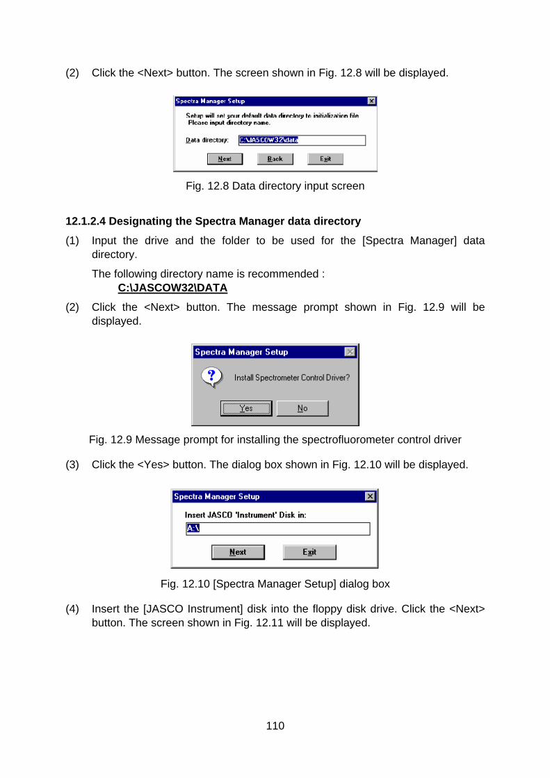
(2) Click the <Next> button. The screen shown in Fig. 12.8 will be displayed.
Fig. 12.8 Data directory input screen
12.1.2.4 Designating the Spectra Manager data directory
(1) Input the drive and the folder to be used for the [Spectra Manager] data directory.
The following directory name is recommended : C:\JASCOW32\DATA
(2) Click the <Next> button. The message prompt shown in Fig. 12.9 will be displayed.
Fig. 12.9 Message prompt for installing the spectrofluorometer control driver
(3) Click the <Yes> button. The dialog box shown in Fig. 12.10 will be displayed.
Fig. 12.10 [Spectra Manager Setup] dialog box
(4) Insert the [JASCO Instrument] disk into the floppy disk drive. Click the <Next> button. The screen shown in Fig. 12.11 will be displayed.
110

Fig. 12.11 Confirmation of the control driver screen
(5) Click the <Continue> button. The screen shown in Fig. 12.12 will be displayed.
Fig. 12.12 Model name and serial number input screen
(6) Input the model name and serial number if necessary, and click the <Next> button.
12.1.2.5 Copying files to the hard disk
The [Setup] program copies the [Spectra Manager] program and related files to the hard disk. As these files are copied, the [Setup] program may request that the operator insert disks into the floppy disk drive. If this happens, click <OK> after the appropriate disk has been inserted into the drive.
After all of the files have been copied, the [Setup] program creates a Jasco folder in the Programs menu. A dialog box will then be displayed, indicating that installation is complete. Click <OK>.
111

12.2 Designating the Serial Port (RS-232C) The serial port default value is [COM1]. If the spectrofluorometer is controlled through another port, the serial port number must be changed using the following procedure:
Fig. 12.13 [Spectra Manager] window
(1) Select [Instruments] - [Port Setting] from the [Spectra Manager] menu. The dialog box shown in Fig. 12.1 will be displayed.
Fig. 12.14 [Port Setting] dialog box
(2) Select the desired serial port, and then click <OK>. The selected serial port is now designated as the serial port used to control the spectrofluorometer.
112