model behaviour: the evolution of strategic transport models?

Model Behaviour: The Evolution of Strategic Transport Models?

Stuart Donovan

20 June, 2019

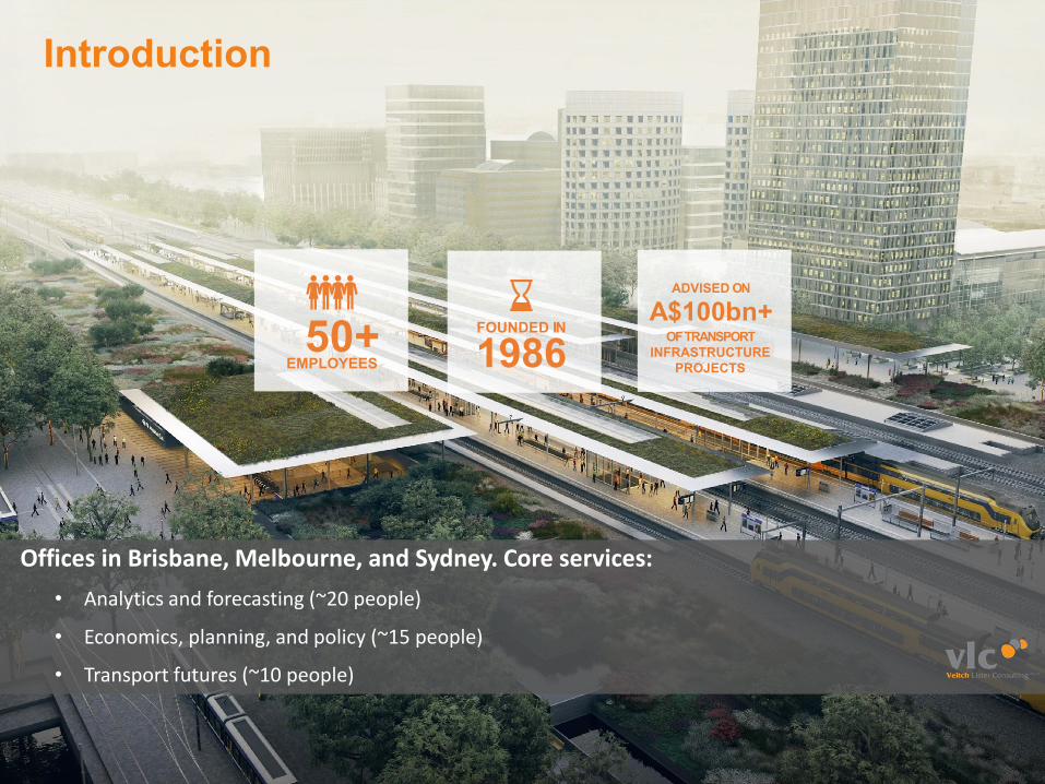
Offices in Brisbane, Melbourne, and Sydney. Core services:• Analytics and forecasting (~20 people)

• Economics, planning, and policy (~15 people)

• Transport futures (~10 people)

EMPLOYEES50+ 1986

FOUNDED IN

ADVISED ON

A$100bn+OF TRANSPORT

INFRASTRUCTURE PROJECTS

Introduction

Introduction

Transport models inform (1) high level policy / strategy and (2) project planning and business cases.

Questions:• What sorts of behavioural responses are modelled?• Do these responses align with key areas of policy?• How might strategic models evolve?

NB: Our research in this area is ongoing; the views herein are presented for “discussion purposes” only.

Strategic transport models

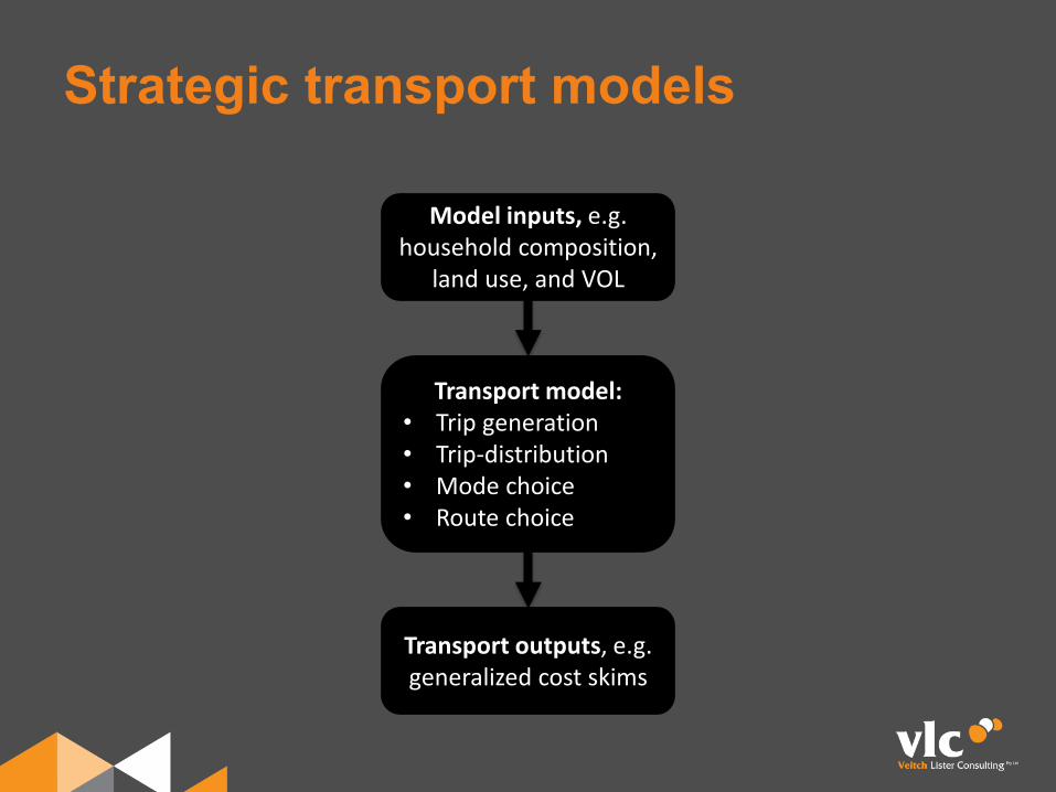
Transport model:• Trip generation• Trip-distribution• Mode choice• Route choice

Transport outputs, e.g. generalized cost skims

Model inputs, e.g. household composition,

land use, and VOL

Behavioural Responses

Conventional strategic transport models typically include three main behavioural responses, specifically:1. Route choice2. Transport mode choice3. Destination choice (sometimes)

Q. What responses are missing?


Strategic transport models typically do not include:1. Trip scheduling2. Location choice3. Vehicle ownership choices4. Travel substitution5. Supply-chains

Q. Are these important?

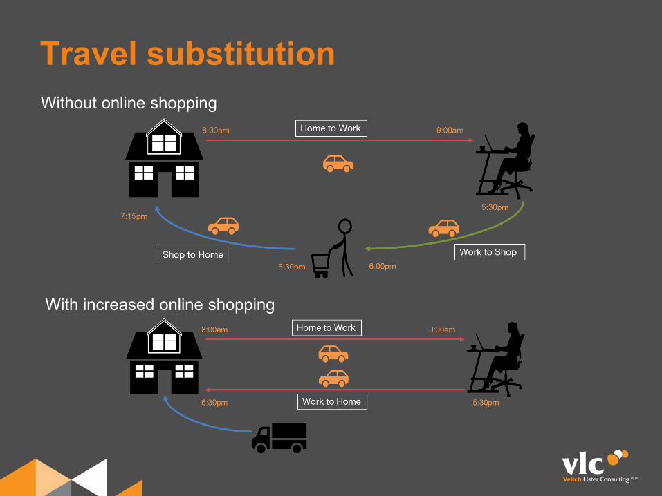
Travel substitutionWithout online shopping

With increased online shopping

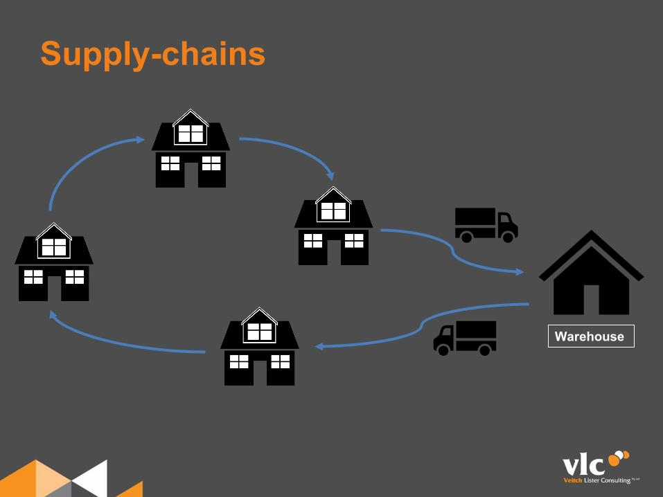
Supply-chains

Warehouse


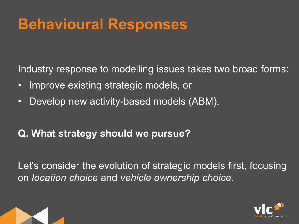
Industry response to modelling issues takes two broad forms:• Improve existing strategic models, or• Develop new activity-based models (ABM).

Q. What strategy should we pursue?

Let’s consider the evolution of strategic models first, focusing on location choice and vehicle ownership choice.

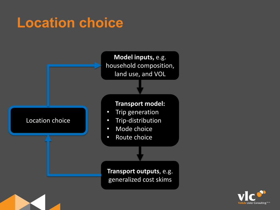
Location choice




land use, and VOL

Location choice

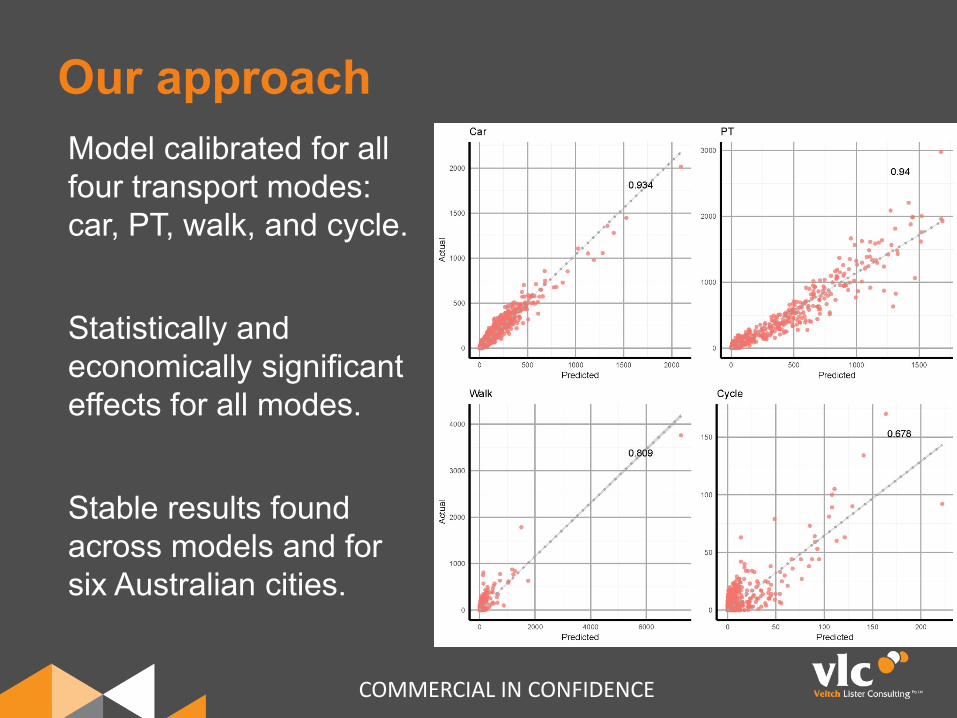
Our approach

COMMERCIAL IN CONFIDENCE

Model calibrated for all four transport modes: car, PT, walk, and cycle.

Statistically and economically significant effects for all modes.

Stable results found across models and for six Australian cities.

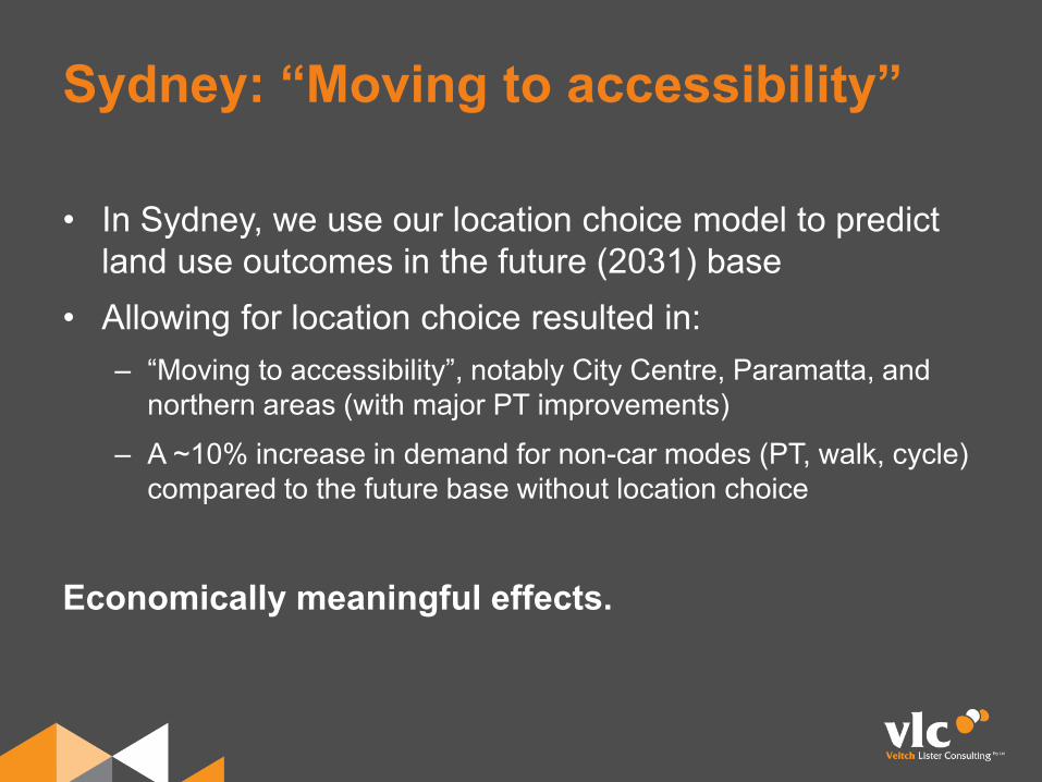
Sydney: “Moving to accessibility”

• In Sydney, we use our location choice model to predict land use outcomes in the future (2031) base

• Allowing for location choice resulted in:– “Moving to accessibility”, notably City Centre, Paramatta, and

northern areas (with major PT improvements)– A ~10% increase in demand for non-car modes (PT, walk, cycle)

compared to the future base without location choice

Economically meaningful effects.

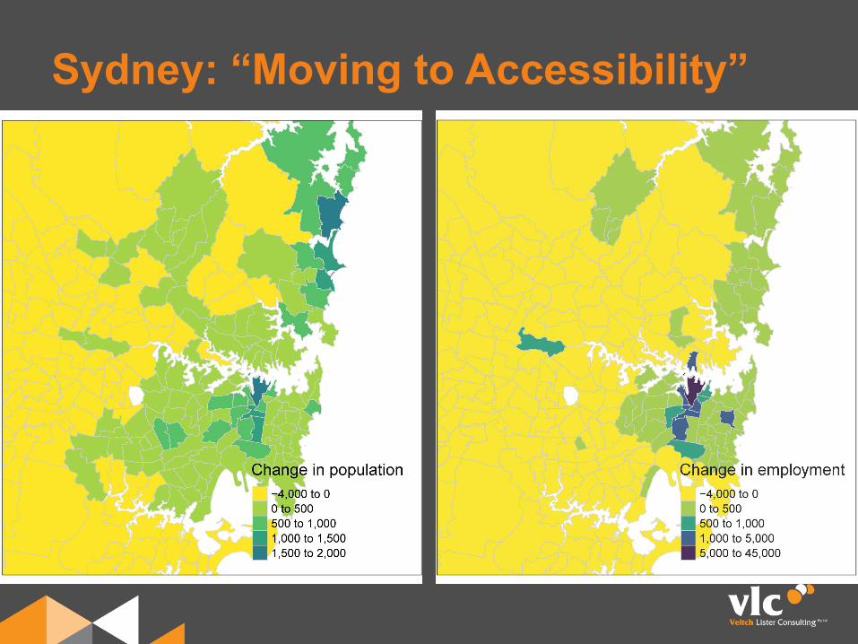
Sydney: “Moving to Accessibility”

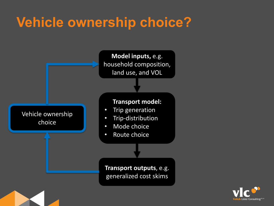
Vehicle ownership choice?




land use, and VOL

Vehicle ownership choice

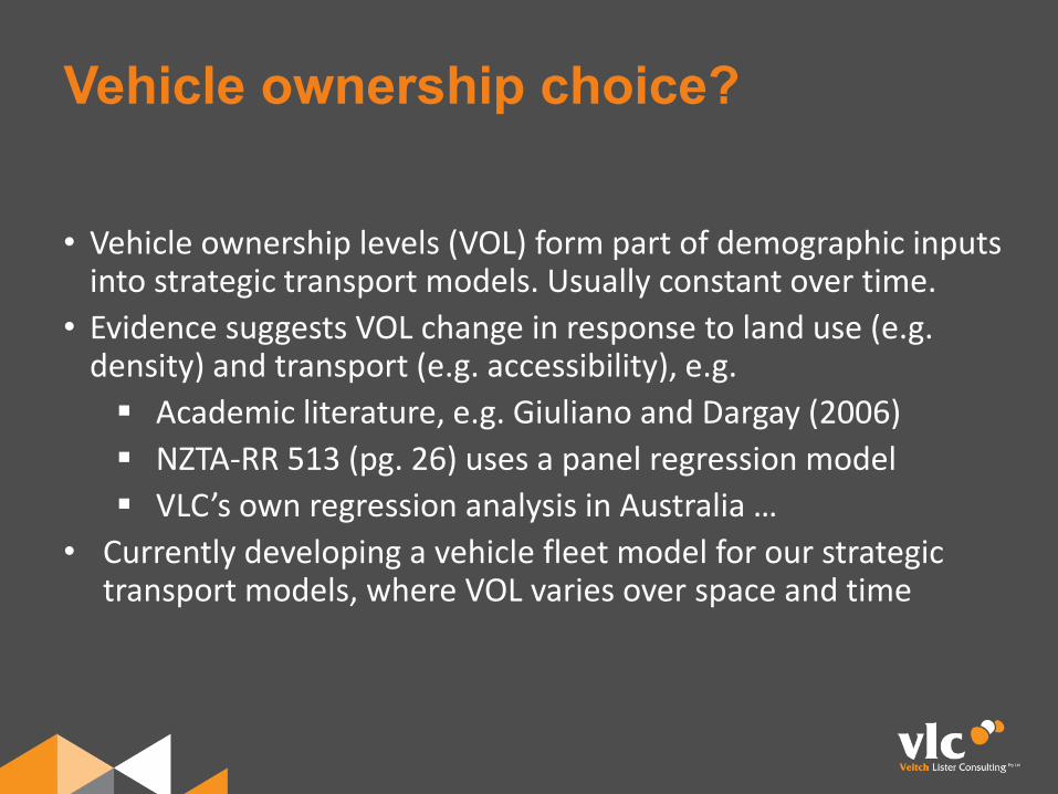
• Vehicle ownership levels (VOL) form part of demographic inputs into strategic transport models. Usually constant over time.

• Evidence suggests VOL change in response to land use (e.g. density) and transport (e.g. accessibility), e.g. Academic literature, e.g. Giuliano and Dargay (2006) NZTA-RR 513 (pg. 26) uses a panel regression model VLC’s own regression analysis in Australia …

• Currently developing a vehicle fleet model for our strategic transport models, where VOL varies over space and time

Vehicle ownership choice?

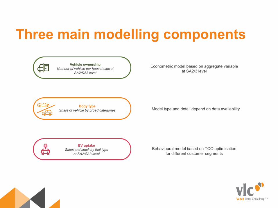
Three main modelling components

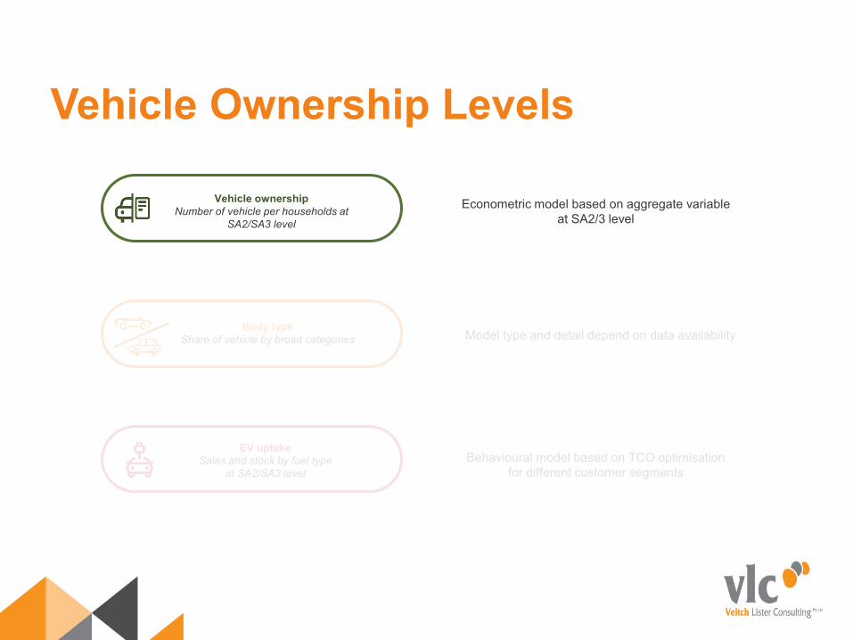
Vehicle ownershipNumber of vehicle per households at

SA2/SA3 level

Body typeShare of vehicle by broad categories

EV uptakeSales and stock by fuel type

at SA2/SA3 level

Model type and detail depend on data availability

Econometric model based on aggregate variable at SA2/3 level

Behavioural model based on TCO optimisation for different customer segments

Vehicle Ownership Levels


SA2/SA3 level



at SA2/SA3 level




Vehicle ownership

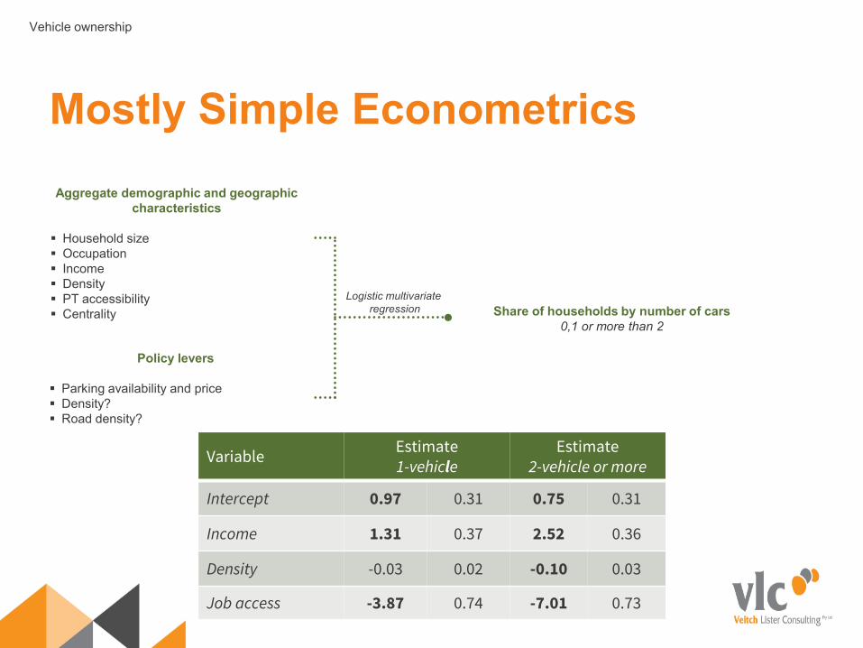
Mostly Simple EconometricsAggregate demographic and geographic

characteristics

Household size Occupation Income Density PT accessibility Centrality

Policy levers

Parking availability and price Density? Road density?

Share of households by number of cars0,1 or more than 2

Logistic multivariate regression

Variable Estimate1-vehicle

Estimate2-vehicle or more

Intercept 0.97 0.31 0.75 0.31

Income 1.31 0.37 2.52 0.36

Density -0.03 0.02 -0.10 0.03

Job access -3.87 0.74 -7.01 0.73

Vehicle ownership

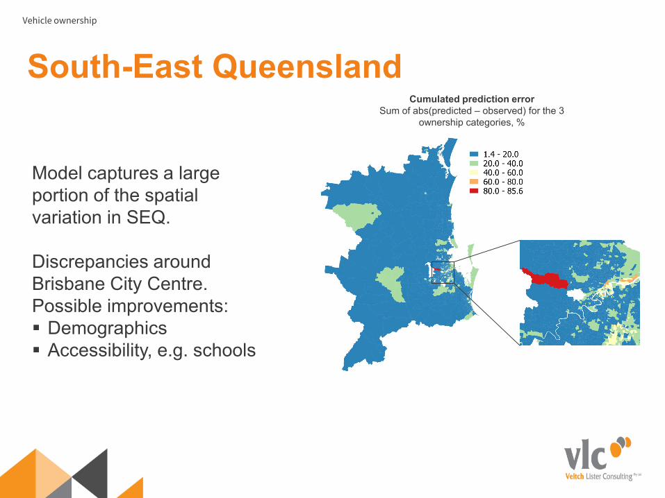
South-East Queensland

Model captures a large portion of the spatial variation in SEQ.

Discrepancies around Brisbane City Centre. Possible improvements: Demographics Accessibility, e.g. schools

Cumulated prediction errorSum of abs(predicted – observed) for the 3

ownership categories, %

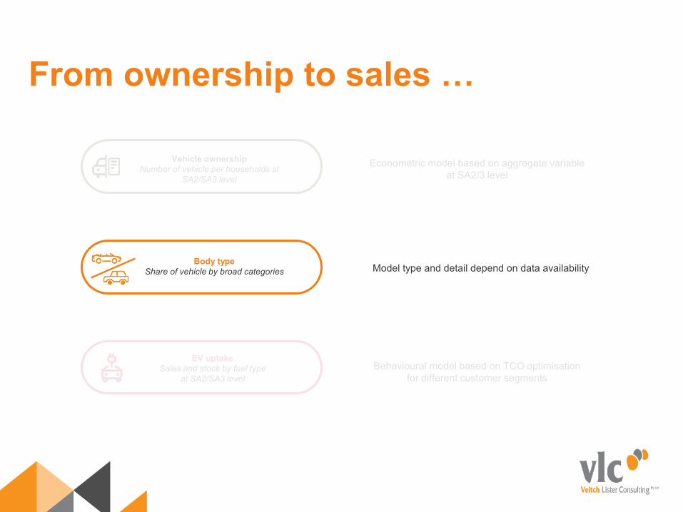
From ownership to sales …


SA2/SA3 level



at SA2/SA3 level




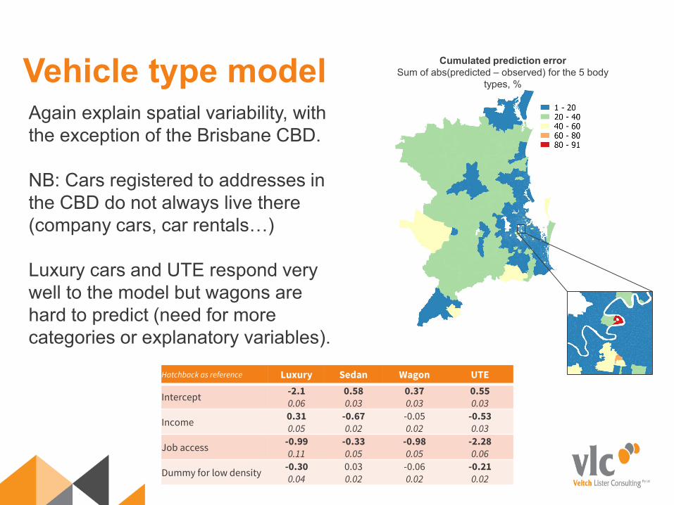
Vehicle type modelAgain explain spatial variability, with the exception of the Brisbane CBD.

NB: Cars registered to addresses in the CBD do not always live there (company cars, car rentals…)

Luxury cars and UTE respond very well to the model but wagons are hard to predict (need for more categories or explanatory variables).

Cumulated prediction errorSum of abs(predicted – observed) for the 5 body

types, %

Hatchback as reference Luxury Sedan Wagon UTE

Intercept -2.10.06

0.580.03

0.370.03

0.550.03

Income 0.310.05

-0.670.02

-0.050.02

-0.530.03

Job access -0.990.11

-0.330.05

-0.980.05

-2.280.06

Dummy for low density -0.300.04

0.030.02

-0.060.02

-0.210.02

EV uptake

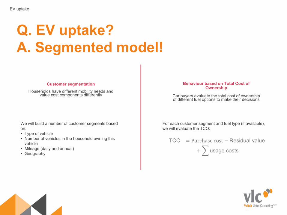
Q. EV uptake?A. Segmented model!

Customer segmentationHouseholds have different mobility needs and

value cost components differently

Behaviour based on Total Cost of Ownership

Car buyers evaluate the total cost of ownership of different fuel options to make their decisions

TCO = Purchase cost − Residual value

+�usage costs

We will build a number of customer segments based on: Type of vehicle Number of vehicles in the household owning this

vehicle Mileage (daily and annual) Geography

For each customer segment and fuel type (if available), we will evaluate the TCO:

00.050.10.150.20.250.30.350.40.45

30000

35000

40000

45000

50000

55000

60000

65000

70000

2018 2020 2022 2024 2026 2028 2030 2032 2034

EV uptake

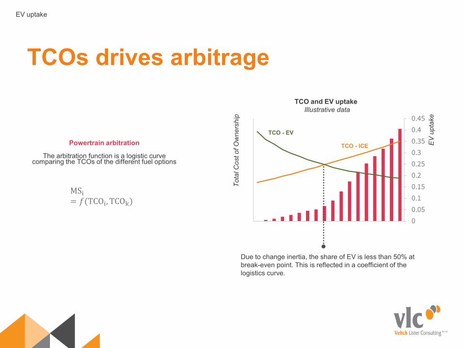
TCOs drives arbitrage

Powertrain arbitration

The arbitration function is a logistic curve comparing the TCOs of the different fuel options

MSi= 𝑓𝑓(TCOi, TCOk)

Due to change inertia, the share of EV is less than 50% at break-even point. This is reflected in a coefficient of the logistics curve.

TCO - EV

TCO - ICE

Tota

l Cos

t of O

wne

rshi

p

EV

upt

ake

TCO and EV uptake Illustrative data

EV uptake

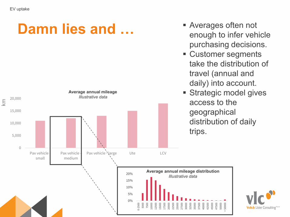
Damn lies and … Averages often not enough to infer vehicle purchasing decisions. Customer segments

take the distribution of travel (annual and daily) into account. Strategic model gives

access to the geographical distribution of daily trips.

0

5,000

10,000

15,000

20,000

Pax vehicle -small

Pax vehicle -medium

Pax vehicle - large Ute LCV

km

0%

5%

10%

15%

20%

0-25

0050

0075

0010

000

1250

015

000

1750

020

000

2250

025

000

2750

030

000

3250

035

000

3750

040

000

4250

045

000

4750

050

000

> 50

000

Average annual mileageIllustrative data

Average annual mileage distributionIllustrative data

Activity based models

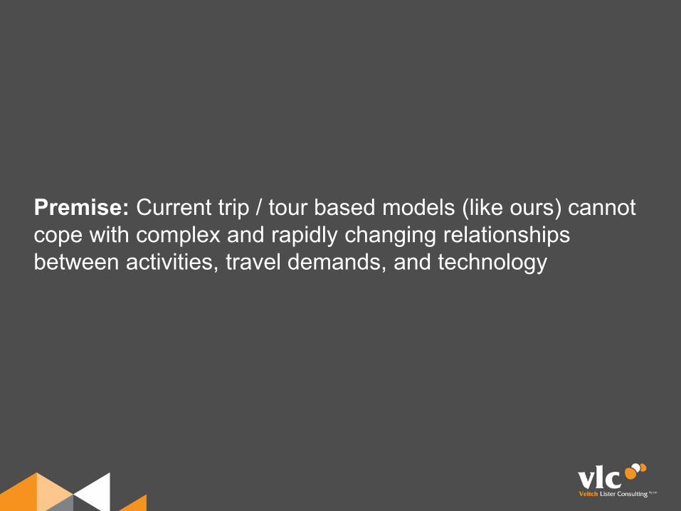
Premise: Current trip / tour based models (like ours) cannot cope with complex and rapidly changing relationships between activities, travel demands, and technology

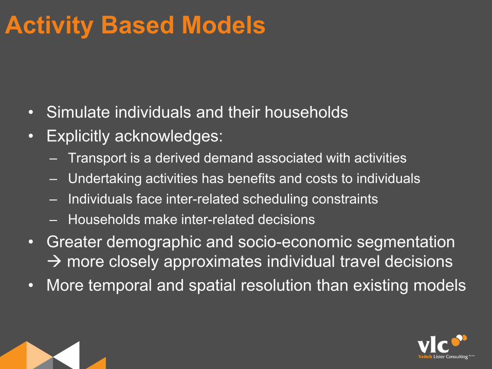
• Simulate individuals and their households• Explicitly acknowledges:

– Transport is a derived demand associated with activities– Undertaking activities has benefits and costs to individuals– Individuals face inter-related scheduling constraints – Households make inter-related decisions

• Greater demographic and socio-economic segmentation more closely approximates individual travel decisions

• More temporal and spatial resolution than existing models

Activity Based Models

Behavioural responses

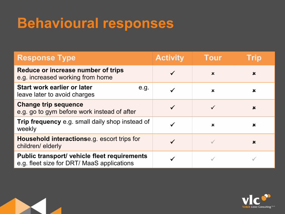
Response Type Activity Tour TripReduce or increase number of trips e.g. increased working from home

Start work earlier or later e.g. leave later to avoid charges

Change trip sequence e.g. go to gym before work instead of after

Trip frequency e.g. small daily shop instead of weekly

Household interactionse.g. escort trips for children/ elderly

Public transport/ vehicle fleet requirements e.g. fleet size for DRT/ MaaS applications

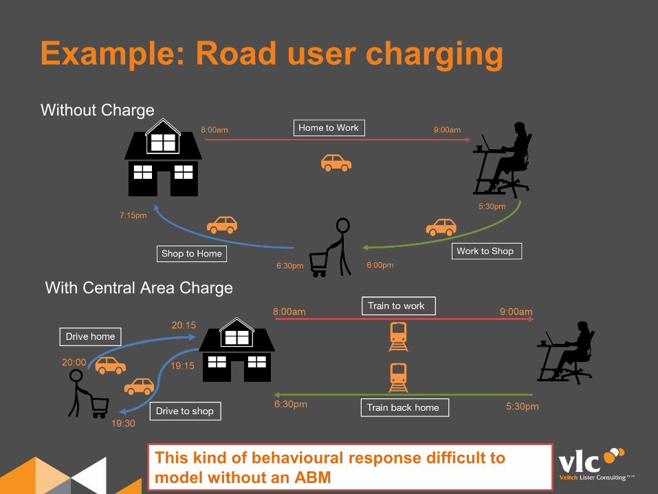
Example: Road user chargingWithout Charge

This kind of behavioural response difficult to model without an ABM

With Central Area Charge

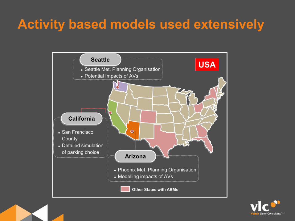
Activity based models used extensively

Seattle Seattle Met. Planning Organisation Potential Impacts of AVs

Arizona

Phoenix Met. Planning Organisation Modelling impacts of AVs

California

San Francisco County

Detailed simulation of parking choice

USA

Other States with ABMs

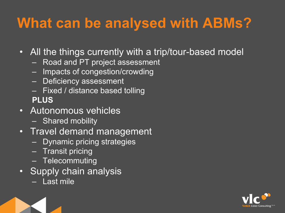
What can be analysed with ABMs?

• All the things currently with a trip/tour-based model– Road and PT project assessment– Impacts of congestion/crowding – Deficiency assessment– Fixed / distance based tollingPLUS

• Autonomous vehicles– Shared mobility

• Travel demand management– Dynamic pricing strategies– Transit pricing– Telecommuting

• Supply chain analysis– Last mile

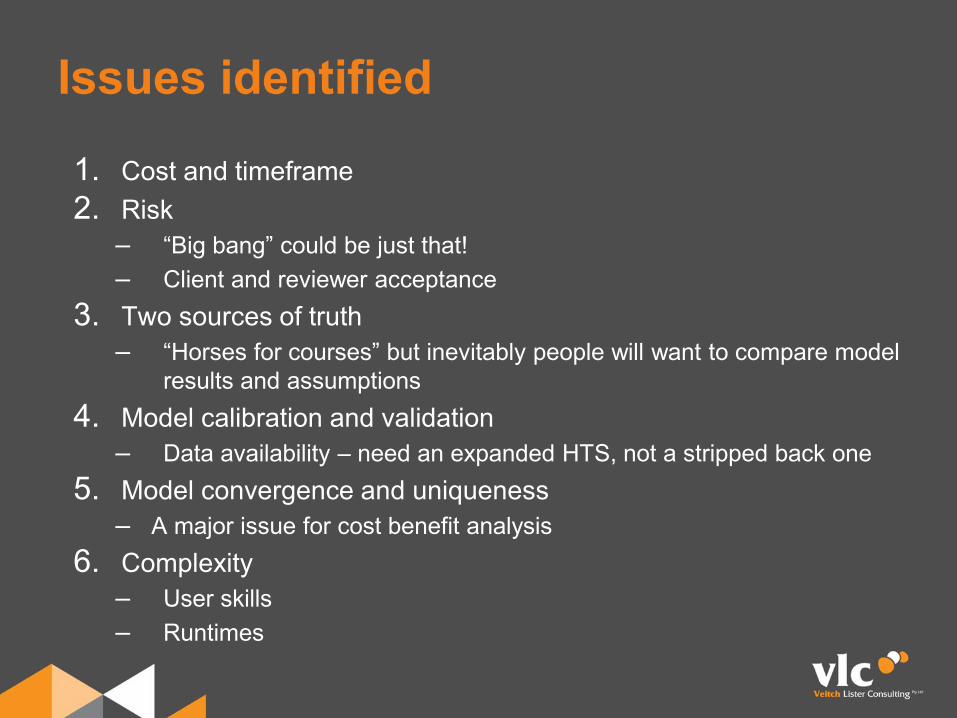
Issues identified

1. Cost and timeframe2. Risk

– “Big bang” could be just that!– Client and reviewer acceptance

3. Two sources of truth– “Horses for courses” but inevitably people will want to compare model

results and assumptions4. Model calibration and validation

– Data availability – need an expanded HTS, not a stripped back one5. Model convergence and uniqueness

– A major issue for cost benefit analysis6. Complexity

– User skills– Runtimes

Contacts

Stuart Donovan [email protected] Gavin Nicholls [email protected]

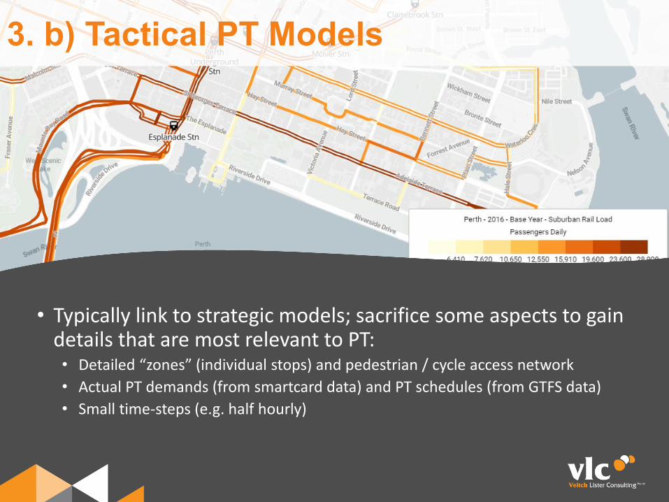
• Typically link to strategic models; sacrifice some aspects to gain details that are most relevant to PT:• Detailed “zones” (individual stops) and pedestrian / cycle access network• Actual PT demands (from smartcard data) and PT schedules (from GTFS data)• Small time-steps (e.g. half hourly)

3. b) Tactical PT Models

model behaviour: the evolution of strategic transport models?

Documents