evolution and sub-optimal behaviour
TRANSCRIPT

Draft: 03/09/2002 3:04 PM
EVOLUTION AND SUB-OPTIMAL BEHAVIOUR
by
Ian M . Dobbs
and
Ian M olho* Acknowledgements: Thanks are due to the anonymous referees for comments which have materially improved the paper. The usual disclaimer applies. *Respectively, Newcastle School of Management and Department of Economics, University of Newcastle upon Tyne, NE1 7RU, England.
KEYWORDS: Suboptimal behaviour, Evolutionary Stability, Sexual Inheritance, Assortative Mating, Population Dynamics.
JEL CLASSIFICATION: D00, D89

2
ABSTRACT
The apparently sub-optimal behaviour of economic agents in games against nature can
be seen as a natural outcome of evolutionary processes. This paper extends previous
work on the evolutionary stability of sub-optimal adaptations by examining how
stability is affected by the introduction of multiple traits and assortative mating. It is
shown that increasing the number of traits tends to increase the scope for stable second
best adaptations whilst assortative mating reduces it. Various economic applications
are discussed.
3
I INTRODUCTION
The traditional neoclassical approach to decision making, whether it be under certainty,
uncertainty, or in strategic situations, has been to postulate that individual agents have
preferences which satisfy some given axiomatic structure (one which induces a
preference ordering) and an infinite calculating capacity when it comes to the problem
of optimisation, of deciding on the best choice subject to the informational and financial
constraints they face. The validity of this ‘utility maximising’ model of human
behaviour has long been subject to debate, and a wealth of experimental studies
showing apparently systematically perverse economic behaviour has served to heighten
this unease (see, for example, Kagel and Roth [1995]).
Although some have advocated an abandonment of the notion of ‘optimising
behaviour’ , preferring to emphasise satisficing in the face of limited calculation power
and bounded rationality (e.g. Simon [1982]), the dominant response to the empirical
challenge has been to look for alternative assumptions or preference structures. Often
such models retain some form of preference functional that the individual is assumed to
maximise (e.g. Kahneman and Tversky [1979], Machina [1979], Viscusi [1989])
although not always (e.g. Loomes and Sugden’s [1982] regret theory). What this
burgeoning literature has in common is that it follows the traditional neoclassical line of
not enquiring too deeply into why individuals have the tastes, attitudes, preference
structures etc. described.
By contrast, recent work in evolutionary economics has begun to address this question.
It is clearly an incontrovertible fact that humans as biological organisms have been

4
subject to a long process of evolution. Early writings by economists on how evolution
might influence individual behaviour and decision making tended to assume it might
well produce the optimising agents of Neoclassical theory, since 'bad' decision-making
seemed unlikely to favour long term survival (e.g. Friedman [1953]). However, more
recent work in this area has shown how it is possible that 'bad' decision making can be
consistent with evolutionary stability. Much of this work focuses on the strategic
interaction between agents. For example, Stahl [1993] advances the argument that
evolutionary forces need not lead to ‘ intelligent’ behaviour, on the grounds that ‘being
right is just as good as being smart’ , whilst Vega-Redondo [1997] shows how
evolution can lead to the play of strategies that are not best responses in games (due to
spiteful behaviour, an idea presaged in earlier work by Alchian [1950]). However,
whilst it is not so surprising that in strategic settings, sub-optimising behaviour may
prove evolutionarily stable, it is somewhat less obvious that this might be the case in
one person decision-making (games against nature). Nevertheless, as Waldman [1994]
has shown, once fecundity is modelled as a sexual, as opposed to an asexual, process,
then even in one person decisions, there are evolutionary arguments which support the
potential for sub-optimal decision-making in steady state (and of course, much of the
experimental literature calling into question the concept of homo economicus does
concern such one-person games against nature).
There is of course a substantial biological literature on population genetics which shows
how types that are sub-optimally adapted to their environment can survive (e.g. Hartl
and Clark [1989]1) and a further literature on genetic algorithms (e.g. Goldberg
1 This text provides a good introduction to the literature. For some specific models, see for example Moran [1964], Ewens [1968] or Karlin [1975].

5
[1989]) which focuses on the ability of genetic systems (incorporating stochastic
elements) to discover global optima. Waldman’s contribution contrasts with the former
literature on population genetics in that it investigates stability with respect to the more
demanding game theory notion of mutant invasion (i.e. whether a dominant population
of sub-optimal adaptations can remain dominant in the face of such invasions). His
analysis also poses something of a challenge to the latter literature on genetic
algorithms, since his results imply that even if a genetic system produces a mutant type
that is optimally adapted to the environment, it remains the case that natural selection
may reject this type in favour of pre-existing sub-optimal adaptations.
Waldman’s analysis focuses on the role of sexual inheritance in generating steady states
in which the dominant type in a population is sub-optimally adapted to its environment
(i.e. not the ‘ fittest’ that could have survived). In his example, types within the
population have just two inherited traits; one particular type combines traits in an
evolutionarily globally optimal way (the 'first best adaptation') whilst another is locally
optimal in that a change in any single trait reduces evolutionary fitness (the 'second best
adaptation').2 If the second best are dominant in the population, then an invasion of
first best types may fail to achieve dominance simply because their seed are dispersed
over existing second best types, so producing cross-breed progeny who are typically
even less fit.
2 We have chosen to stick with term 'second best' adaptation, as described here, as it has been previously established in the literature. However, it should be noted that a second best adaptation may rank well below second in terms of fitness (as in the final example in section III below) and 'second best' also carries other connotations for economists. For a formal definition of 'second best adaptation' see section II.

6
Waldman assumed that evolutionary types have just two inherited traits and that sexual
matching of types is purely random. The contribution of the present paper is to extend
this analysis to the more general case where there can be an arbitrary number of traits
and, in addition, a variable degree of assortative mating. Multiple (>2) inherited traits
and assortative mating both reflect real world phenomena. Firstly, most organisms
(including humans) differ in an enormous variety of ways that are both inherited and
relevant to evolutionary fitness. Secondly, humans display outward manifestations of
type differences (height, weight, hair, skin, language etc.) and feature local
concentrations (by country, area, occupation, social circle, religious affiliation etc.).
These factors, or traits, clearly lead to non-random mating and breeding, with an above
average frequency of ‘own-type’ mating being the norm.
In section II, it is shown that, on introducing multiple (>2) traits, the concept of a
second best adaptation (SBA) remains central to the question of whether a sub-optimal
type can be evolutionarily stable or not (being a SBA is a necessary condition for
evolutionary stability). It is also shown that the increase in the number of traits raises
the scope for stable second best adaptations, whilst breeding selectivity reduces it.
Section III then provides some economic examples illustrating the relevance of the
stability analysis, whilst section IV concludes by discussing the intuition for the results.
II POPULATION DYNAMICS AND SECOND BEST STABILITY It is assumed that evolutionary types live for one period, that there are two genders
(equal in number for each type) and that fecundity is determined solely by the traits of

7
the female type, as in Waldman [1994]. Types are characterised by a vector of n traits
a = a a an1 2, ,..,� �
∈ A where A denotes a set of admissible trait vectors. The growth
rate from one generation to the next, for a type with trait vector a, is given by the
function k a k a a an( ) , ,..,≡ 1 2
� �. For simplicity, we assume that types can be strictly
ordered in terms of fecundity (i.e. no ties: for types a, b, a b≠ , then k a k b( ) ( )≠ ).
The definition of a second best adaptation (SBA) is a trait vector asba such that:
k a a a k a a asbarsba
nsba sba
r nsba( ,.., ,.., ) ( ,.., ,.., )1 1> for all a ar r
sba≠ , and all r n= 1,.., . (1) whilst the (assumed unique) first best trait vector is a fba such that
k a k afba( ) ( )> for all a A a a fba∈ ≠, . (2)
Thus the first best is also a SBA (the ‘best of the second best’ ).
A type is said to be evolutionarily stable if a population of this type can remain the
dominant population in the face of a FBA incursion. In the ensuing analysis, it is shown
that any type which is not a SBA is evolutionarily unstable; that is, being a SBA is a
necessary, but not sufficient, condition for evolutionary stability. We then establish
conditions under which a SBA is evolutionarily stable or unstable.
Consider a population of a given type, denoted as faced by an incursion by another
type a f . These types mix and interbreed, with the consequence that 2n different types
are generated amongst the progeny;3 each of these progeny have a trait vector a in
3 Note that, without loss of generality, it can be assumed that for all ar , r=1,..,n, it is
the case that a arf
rs≠ . If some elements were the same, the fecundity function k can be
redefined such that only the elements that differ are represented as arguments. The

8
which the element a ar rs= or ar
f , r=1,..,n. Thus, for the ensuing analysis, the set of
types, A, can be restricted to the set A a a a a r nr rs
rf= ={ : ,.., }= or , 1 . In considering
evolutionary stability, a f is assumed to be a FBA and hence satisfies equation (2) (i.e.
a af fba≡ ), and we consider whether stability requires type as to be a SBA or not.
Types are labelled a ii n, , ,..,= 12 2 so A a an
= 1 2,..,� �
(thus superscripts identify
particular trait-vectors whilst a subscript identifies a particular element in a trait vector;
the way types are labelled is discussed further in the ensuing analysis and in the
appendix). Let p p p pt
a
t
a
t
a
tn= ( , ,.., )1 2 2
denote the vector at time t of proportions of each
type i=1,..,2n. It is convenient to identify a as ≡ 1 and a af n
≡ 2 . Naturally, the
proportions pa
ti , i=1,..,2n sum to unity. Hence we can write
p pa
tat
a A a a
s
s
= −∈ ≠
�1
,
. (3)
In what follows, the evolution of the types a a an2 3 2, ,.., is studied. The evolution of
type a as ≡ 1 is then implicitly determined by (3). Each proportion evolves according to
a difference equation of the type
p f pa
t i ti+ =1 ( ) , i=2,3,..,2n. (4)
where p p p pt
a
t
a
t
a
tn= 2 3 2
, ,..,e j .
point is that for any trait element which is the same for both types, procreation always generates offspring with the same value for that trait element. Thus only those elements which have the potential to change from one generation to the next need be included in the analysis.

9
An equilibrium point in this system, � ( � , � ,.. � )p p p pa a a
n= 2 3 2, is such that
�(
�)p f p
a
ii = ,
i=2,3,..,2n. A sufficient condition for local asymptotic stability for (4) is established if
all the eigenvalues of the Jacobian matrix f pp(�) lie strictly within the unit circle, whilst
a sufficient condition for instability is that at least one of the roots lies outside the unit
circle.4 Thus the type as is evolutionarily stable if the equilibrium (0,0,..,0) is locally
asymptotically stable (note that pa
ti = 0 for i=2,3,..,2n implies p
a
ts = 1, from (3)) and it
is evolutionarily unstable if the equilibrium is unstable. The use of local asymptotic
stability as the equilibrium concept conforms to the standard game theory concept of
‘evolutionarily stable strategies’ (Van Damme [1987]), here applied to a ‘one person’
decision problem.
Assortative mating is modelled by introducing, for each trait vector a A∈ , a parameter
γ ( ) ( , )a ∈ 01 , associated with type a such that a proportion 1-γ ( )a mates with its own
type (and, by assumption, opposite gender!) whilst a proportion γ ( )a mates 'at
random'. Of those that mate at random, some may (by chance) mate with their own
kind, whilst others mate with other types. The proportion of own-type pairing can be
shown to be
( ( )) [( ( ) ) / ]1 2− +γ γa p a p Gat
at t (5)
4See Hofbauer and Sigmund [1988] for a general discussion of evolutionary dynamic systems. For a clear exposition of stability (and instability) theorems for difference equation systems, see Lakshmikantham and Trigiante [1988, ch. 4]. The analysis of stability presented in Waldman [1994] is somewhat imprecise, although the results he obtains are in fact correct.
10
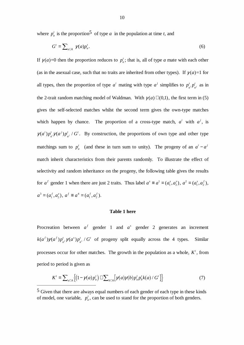
where pat is the proportion5 of type a in the population at time t, and
G a pt
a A at=
∈
�γ ( ) . (6)
If γ ( )a =0 then the proportion reduces to pat ; that is, all of type a mate with each other
(as in the asexual case, such that no traits are inherited from other types). If γ ( )a =1 for
all types, then the proportion of type ai mating with type a j simplifies to p pa
t
a
ti j as in
the 2-trait random matching model of Waldman. With γ ( ) ( , )a ∈ 01 , the first term in (5)
gives the self-selected matches whilst the second term gives the own-type matches
which happen by chance. The proportion of a cross-type match, ai with a j , is
γ γ( ) ( ) /a p a p Gi
a
t j
a
t ti j . By construction, the proportions of own type and other type
matchings sum to pat (and these in turn sum to unity). The progeny of an a ai j−
match inherit characteristics from their parents randomly. To illustrate the effect of
selectivity and random inheritance on the progeny, the following table gives the results
for a f gender 1 when there are just 2 traits. Thus label a a a as s s≡ =11 2( , ), a a as f2
1 2= ( , ),
a a af s31 2= ( , ), a a a af f f≡ =4
1 2( , ).
Table 1 here
Procreation between a f gender 1 and as gender 2 generates an increment
k a a p a p Gf f
a
t s
a
t tf s( ) ( ) ( ) /γ γ of progeny split equally across the 4 types. Similar
processes occur for other matches. The growth in the population as a whole, K t , from
period to period is given as
K a p a b p p k a Gtat
at
bt t
b Aa A= − +
∈∈ �� 1 γ γ γa fc h a f a f a fo t/ (7)
5 Given that there are always equal numbers of each gender of each type in these kinds of model, one variable, pa
t , can be used to stand for the proportion of both genders.
11
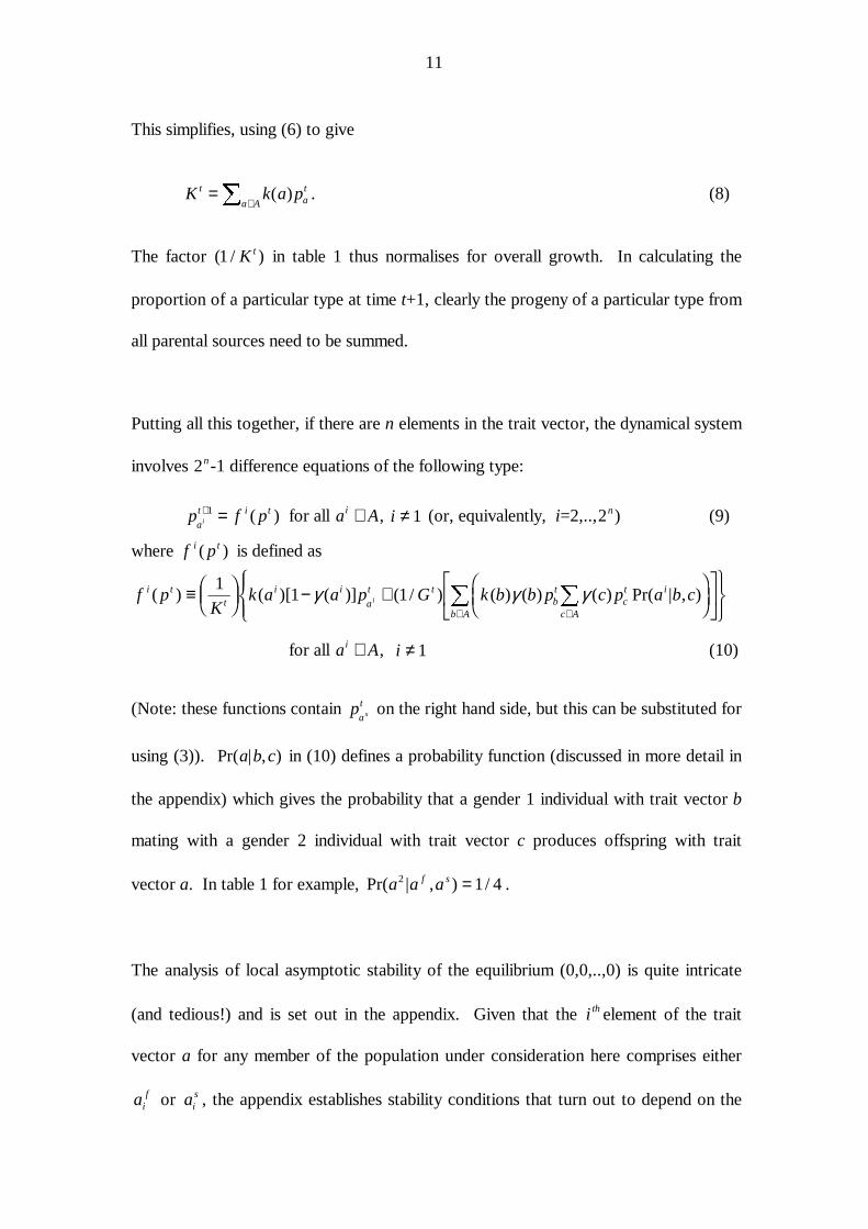
This simplifies, using (6) to give
K k a ptat
a A=
∈
�( ) . (8)
The factor ( / )1 K t in table 1 thus normalises for overall growth. In calculating the
proportion of a particular type at time t+1, clearly the progeny of a particular type from
all parental sources need to be summed.
Putting all this together, if there are n elements in the trait vector, the dynamical system
involves 2n-1 difference equations of the following type:
p f pa
t i ti+ =1 ( ) for all a Ai ∈ , i ≠ 1 (or, equivalently, i=2,..,2n) (9)
where f pi t( ) is defined as
f pK
k a a p G k b b p c p a b ci tt
i i
a
t tbt
ct i
c Ab A
i( ) ( )[ ( )] ( / ) ( ) ( ) ( ) Pr( | , )≡ FHGIKJ
− + FHG
IKJ
L
NM
O
QP
RS|
T|
UV|
W|∈∈
��11 1γ γ γ
for all a Ai ∈ , i ≠ 1 (10)
(Note: these functions contain p
a
ts on the right hand side, but this can be substituted for
using (3)). Pr( | , )a b c in (10) defines a probability function (discussed in more detail in
the appendix) which gives the probability that a gender 1 individual with trait vector b
mating with a gender 2 individual with trait vector c produces offspring with trait
vector a. In table 1 for example, Pr( | , ) /a a af s2 1 4= .
The analysis of local asymptotic stability of the equilibrium (0,0,..,0) is quite intricate
(and tedious!) and is set out in the appendix. Given that the i th element of the trait
vector a for any member of the population under consideration here comprises either
aif or ai
s , the appendix establishes stability conditions that turn out to depend on the

12
number of elements by which a type differs from that of the FBA (where the order of
elements is of no consequence). Suppose an intermediate type a has m elements the
same as the FBA, and n-m which differ. Denote this information by writing such a type
as a m( ). Then it can be shown (appendix) that sufficient conditions for local stability
are that
k a a m m k a ms( ) ( ) , ( )> θ γ a fb g a f for all a(m) for m=1,2,..,n. (11)
where the function θ γ( , )m is defined as
θ γγ
γ,
( { / } )
{ / }m
m
ma fm r
=− −
−1 1 1 2
1 1 2. (12)
whilst a sufficient condition for instability is that the inequality in (11) is reversed for at
least one of the types.
Setting n=2 (the 2-trait case) and γ (.) = 1 (i.e. random mating for all types), then (11)
generates the sufficient conditions for stability obtained by Waldman; namely that
k a k as( ) ( ( ))> 1 for all a(1) (13)
k a k as f( ) ( ) /> 3 (14)
where there are two half-breeds; i.e. the set of a( )1 types comprises ( , )a af s1 2 and
( , )a as f1 2 . Again, a sufficient condition for instability is that at least one inequality is
reversed.
In the n-trait case, when m=1, then (12) simplifies to give θ = 1 and so stability requires
that
k a k as( ) ( )> 1a f for all a(1). (15)
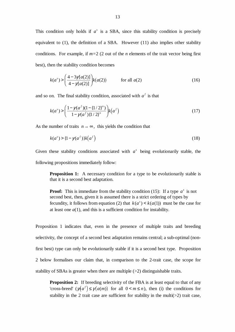
13
This condition only holds if as is a SBA, since this stability condition is precisely
equivalent to (1), the definition of a SBA. However (11) also implies other stability
conditions. For example, if m=2 (2 out of the n elements of the trait vector being first
best), then the stability condition becomes
k aa
ak as( )
[ ( )]
[ ( )]( )> −
−FHG
IKJ
4 3 2
4 22
γγ
a f for all a( )2 (16)
and so on. The final stability condition, associated with a f is that
k aa
ak as
f n
f nf( )
( )( { / } )
( ){ / }> − −
−FHG
IKJ
1 1 1 2
1 1 2
γγ c h (17)
As the number of traits n→ ∞ , this yields the condition that
k a a k as f f( ) { ( )}> −1 γ � � (18)
Given these stability conditions associated with as being evolutionarily stable, the
following propositions immediately follow:
Proposition 1: A necessary condition for a type to be evolutionarily stable is that it is a second best adaptation. Proof: This is immediate from the stability condition (15): If a type as is not second best, then, given it is assumed there is a strict ordering of types by fecundity, it follows from equation (2) that k a k as( ) ( ( ))< 1 must be the case for at least one a(1), and this is a sufficient condition for instability.
Proposition 1 indicates that, even in the presence of multiple traits and breeding
selectivity, the concept of a second best adaptation remains central; a sub-optimal (non-
first best) type can only be evolutionarily stable if it is a second best type. Proposition
2 below formalises our claim that, in comparison to the 2-trait case, the scope for
stability of SBAs is greater when there are multiple (>2) distinguishable traits.
Proposition 2: If breeding selectivity of the FBA is at least equal to that of any 'cross-breed' (γ γa a mf
� � � �≤ ( ) for all 0 < ≤m n), then (i) the conditions for
stability in the 2 trait case are sufficient for stability in the multi(>2) trait case,

14
but (ii) it is possible for a SBA to be evolutionarily stable in the multi-trait case without it satisfying these conditions. Proof: see Appendix
Note also that propositions 1 and 2 also hold for the special case of random
breeding(when γ a m( )a f=1 for all m).
Increasing own type breeding selectivity reduces the chances of the second best
adaptation being evolutionarily stable. Thus, if we standardise breeding selectivity by
setting γ γa m m( ),b g = for m n= 1,.., , then we have:
Proposition 3: Increasing breeding selectivity (decreasing γ ) reduces the range of second best fecundity which satisfies the sufficient conditions for stability (and increases the range on which it is unstable).
Proof: See Appendix.
However, so long as breeding selectivity is imperfect for the first best, there is always
some scope for SBAs to be evolutionarily stable. As selectivity of the first best
increases, so the scope for SBAs to be stable decreases. Finally, if the first best are
perfectly selective, they are the only type that can be evolutionarily stable:
Proposition 4: If the FBA is imperfectly selective ( 0 1< ≤γ a fc h ), then
evolutionarily stable SBAs may exist. If the FBA is perfectly selective
(γ a fc h = 0), then no evolutionarily stable SBAs exist.
Proof: See Appendix.
Once introduced into the population, a perfectly selective FBA sub-population that
manages to 'keep to itself' will simply grow faster than other types and hence will
eventually come to dominate the population.
If we focus on the random matching case, the stability conditions (11) imply that
k a k as( ) ( )> 1� �
for all a( )1

15
k a k as( ) ( ) /> 2 3� �
for all a( )2
k a k as( ) ( ) /> 3 7� �
for all a( )3
k a k as( ) ( ) /> 4 15� �
for all a( )4
and so on; that is,
k a k a qs q( ) ( ) /> −b g c h2 1 for all a q( ) , 1≤ ≤q n .
This makes clear that, under random mating, although there are a multiplicity of
conditions that must be satisfied for a type to be evolutionarily stable, only the first is
significantly restrictive (in view of the effect of the rapidly increasing size of the term
2 1q −c h ). That is, under random matching, one might expect most SBAs to be stable.
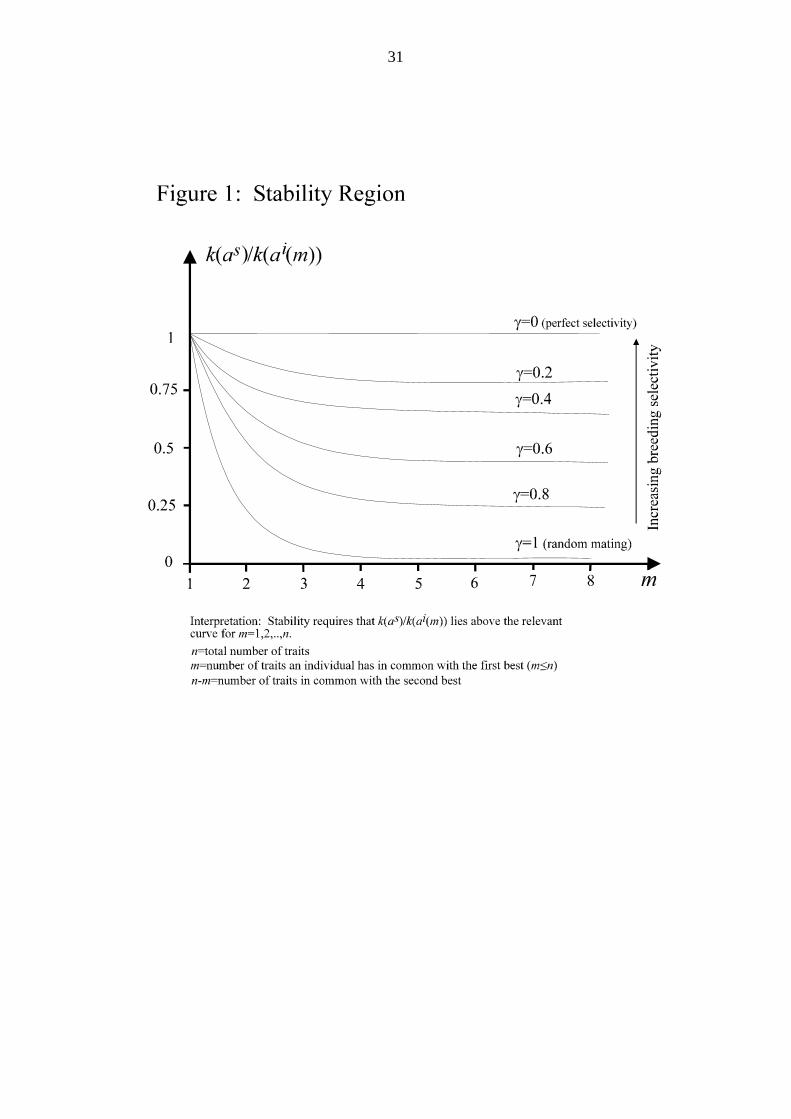
Figure 1 here
Returning to the selective breeding case, figure 1 graphs the value of θ γ( , )m as a
function of γ ,m. Fecundity of the SBA relative to that of a cross-breed with m
elements in common with the FBA and n-m elements in common with the SBA is
measured on the vertical axis. For a SBA to be evolutionarily stable, the relative
fecundity, for each type of cross-breed, must lie above the relevant curve. To interpret
the figure, say γ = 06. and the number of traits is n=4. Then the system is stable if
relative fecundity lies above the γ = 06. curve at the points m = 1, 2, 3, and 4.
Increasing the number of traits n, for example to 5, means that, for stability, relative
fecundity must lie above the curve for types with m = 1, 2, 3, 4, and 5 also. With
higher breeding selectivity, the relevant curves are positioned higher, so the region of
stability is curtailed.
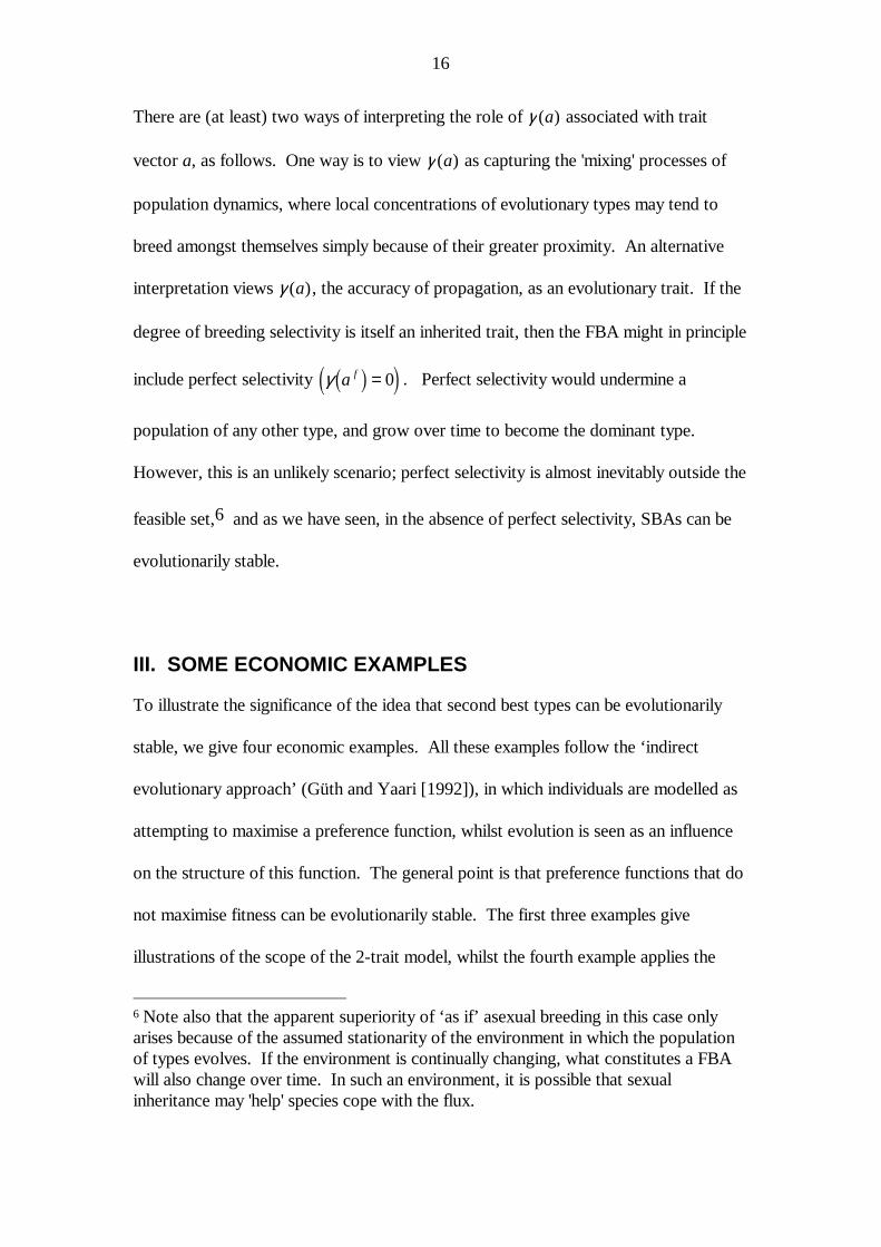
16
There are (at least) two ways of interpreting the role of γ ( )a associated with trait
vector a, as follows. One way is to view γ ( )a as capturing the 'mixing' processes of
population dynamics, where local concentrations of evolutionary types may tend to
breed amongst themselves simply because of their greater proximity. An alternative
interpretation views γ ( )a , the accuracy of propagation, as an evolutionary trait. If the
degree of breeding selectivity is itself an inherited trait, then the FBA might in principle
include perfect selectivity γ a fc he j= 0 . Perfect selectivity would undermine a
population of any other type, and grow over time to become the dominant type.
However, this is an unlikely scenario; perfect selectivity is almost inevitably outside the
feasible set,6 and as we have seen, in the absence of perfect selectivity, SBAs can be
evolutionarily stable.
III. SOME ECONOMIC EXAMPLES To illustrate the significance of the idea that second best types can be evolutionarily
stable, we give four economic examples. All these examples follow the ‘ indirect
evolutionary approach’ (Güth and Yaari [1992]), in which individuals are modelled as
attempting to maximise a preference function, whilst evolution is seen as an influence
on the structure of this function. The general point is that preference functions that do
not maximise fitness can be evolutionarily stable. The first three examples give
illustrations of the scope of the 2-trait model, whilst the fourth example applies the
6 Note also that the apparent superiority of ‘as if’ asexual breeding in this case only arises because of the assumed stationarity of the environment in which the population of types evolves. If the environment is continually changing, what constitutes a FBA will also change over time. In such an environment, it is possible that sexual inheritance may 'help' species cope with the flux.

17
results obtained in section II to a case involving three traits and possibly assortative
mating.
III (a) Over-estimation of Ability
Waldman's [1994] example concerned evolutionary types who inherit one trait for
estimating their own ability and another for their degree of inherent 'laziness' and who
mate at random. The first best type accurately estimates its own ability and is not lazy.
The type who is lazy but over-estimates own ability is a 'second best type' in that a
change in either trait on its own reduces evolutionary fitness. Thus a type who
overestimates ability but is not lazy would choose to work 'too hard' for the good of its
own propagation (since it believes the marginal return to work is greater than it really
is); by contrast, a type who is simply lazy (but does not overestimate ability), would
work too little. Both these types are less 'fit' than the second best. From the stability
results (section II above), it then follows that the second best type, featuring
overestimation and laziness, can be evolutionarily stable.
III (b) Altruism: Economists often view altruistic behaviour as something inconsistent with survival of
the fittest.7 The following analysis illustrates how altruism can be consistent with
second best stability under sexual inheritance. Suppose evolutionary types mate at
random and also generate wealth W according to the function W e= where e is effort
( 0 1≤ ≤e ). The fruits of this effort are publicly enjoyed (in directions which do not
affect fecundity), such that the agent only receives a return π ( 0 ≤ ≤π W ))as private
consumption, whilst W − π is enjoyed by others. Suppose fecundity increases with π,
7 Though studies such as Huck and Oechssler [1998] show that apparently altruistic behaviour may arise in an evolutionary model.

18
and decreases with effort for given π (for example, because the type might 'wear itself
out' by working too hard), such that
k e= + −1 2π . (19)
Now suppose the agent’s utility is a function of private consumption, benefits to others,
and effort, such that
U W e= + − −π α π β( ) , (20)
where the values of α and β are interpreted as inherited traits reflecting altruism and
laziness respectively. Specifically, suppose α = 0 (selfish) or α = 1/3 (altruistic), whilst
β = 2 (relatively hard working) or β = 3/2 (relatively lazy). Finally, suppose the
individual is able to capture only one half of the wealth W as private consumption, the
other half being enjoyed by others. Thus π = 12W . Hence the utility function
simplifies to
U e e= + −12 1 α β
� �. (21)
Solving this for optimal effort level e* gives
e* //
= +−
1 21 1α β β
b g � � . (22)
Plugging in the values for α β, then gives the ordering of evolutionary types as
described in table 2.
Table 2 here
Thus, altruism induces the individual to work harder (since she gains utility from the
wealth others get as well as her own) whilst laziness induces lower effort. The two
together tend to cancel each other out such that effort is close to optimal. A change in
any one trait at a time leads to an evolutionarily worse outcome, so the slothful altruist
can be a second best type which is evolutionarily stable. In fact, this second best

19
adaptation is evolutionarily stable, since the fecundity of the second best satisfies
stability conditions (13) and (14).
III (c) Risk aversion: Suppose evolutionary types mate at random and face the following gamble: they must
decide on an effort level e, and receive income π in direct proportion to effort, such
that π = e, although this is received only with probability 0.75 (otherwise they receive
zero). Further, suppose (cf. III(b) above) fecundity depends on expected income, but
decreases with effort given income, such that
k e e= + −09 075 2. . . (23)
Finally, suppose that an individual’s von Neumann-Morgenstern utility function is
U e= −π α β . Thus, expected utility is
EU e e e= − + − = −075 025 0 075. . .π πα β β α βc h c h , (24)
where the value of α is interpreted as an inherited trait for risk aversion taking values α
=1 or α=1/2 whilst β is a trait for laziness taking values β = 2 or β = 2.25. Maximising
expected utility gives optimal effort
e* / ./= −β α α β
0751
b g ��. (25)
Plugging values for α β, into (25) gives effort levels and then (23) gives fecundities;
this yields an ordering for the fecundity of evolutionary types as given in table 3.
Table 3 here
Here, the first best is risk neutral, but not a 'workaholic'. The second best type is a risk
averse workaholic. Once again a change in either trait reduces evolutionary fitness and
this 'risk averse workaholic' satisfies the stability condition (11) and so is evolutionarily
stable.

20
III (d) Stupidity, Impatience and Sloth The above applications all related to a world of two inherited traits and random
breeding. The following example utilises the results of section II on multiple (>2)
traits and breeding selectivity.
Suppose types live two periods8 and make an investment decision in the first period
which involves costly effort e but which yields a payoff π t , t=1,2 given as:
π α1 = e, π α2 = g e, (26)
where α is an inherited trait reflecting ability and g is a growth factor; g>1 suggests that
the initial effort generates an increasing return over time from the initial investment in
effort e. Lifetime fecundity is given as:
k w w w w w e= + + + −0 1 1 2 2 3 42π π α , (27)
where w ii > =0 0 4, ,.., are given constants. Thus both ability, and returns (in both
periods), positively influence fecundity whilst effort per se reduces it.9 and the squared
effort term reflects the adverse effect of effort on fecundity. Lifetime utility is given as:
U e= + −π δπ β1 22 , (28)
where δ and β (>0) are inherited traits for patience and sloth respectively. Utility
maximisation yields an optimal effort level
8 We assume for simplicity that types mate for life; the two periods discussed above lie within the period of the procreative cycle. 9 Returns available for consumption in period 1 could be seen as having either a greater or a lesser impact in terms of success in getting progeny through to the point where they become adults who then enter the procreative cycle. It is possible to produce similar results to those reported with the coefficient on π 2 being greater or less than that on π 1.

21
e g* /= +α δ β1 2b g . (29)
In what follows we give a numerical illustration for the case where g=1.1,
w w w w w0 1 2 3 41
21= = = = =, and the inherited traits can take on the discrete values α
= 1.5 or 0.8 (‘able’ or ‘stupid’), β = 0.3 or 0.8 (‘workaholic’ or ‘sloth’), and δ = 0.5 or
0.8 (impatient or patient). The implied choices and fecundity for the various different
types are given below:
Table 4 here
It turns out that the first best is the ‘able, short termist, workaholic’ , whilst the ‘stupid,
patient, sloth’ is a second best. Thus the first best has the highest fecundity, whilst the
second best has a higher fecundity than any adaptation which differs from it in just one
element in the trait vector (although note it has only third highest fecundity). Now,
consider the stability of the stupid-impatient-workaholic second best type; sufficient
conditions for stability of the SBA indicate that this type is evolutionarily stable if
(i) fecundity k for the second best type (with m=0) is greater than that for
types with m=1; i.e. k a k a k as( ) ≡ >0 1� �� � � �� �
. This condition
automatically holds given the definition of a SBA (see table 4).
(ii) the fecundity of the second best type is not 'too low' relative to that of types
that differ in two traits ( m= 2) ; thus stability requires that
4 2 4 3 2 2− > −γ γa k a a k asb gc h c h b gc h b gc h for all types a(2) having two
traits different from the first best. This automatically holds for those a( )2
for which k a k asc h b g> ( )2 . However, the ‘stupid, impatient, workaholic’
(siw for short) type has a higher fecundity than the ‘stupid patient sloth’
SBA. Thus SBA stability requires 4 4 3− > −γ γsiws
siw siwk k where
k s = 16254. and ksiw = 182444. . This holds so long as γ siw > 0207. (recall
that random mating would involve γ siw = 1 whilst perfect selectivity implies
γ siw = 0).

22
(iii) Fecundity is not too low compared to that of the first best ( )m= 3 . From
(17), the condition is that k k ks
f
f
ff
ff>
− −
−= −
−
1 1
1
8 7
8
12
3
12
3
d iγγ
γγ
where
k f = 232344. and k s = 16254. . Rearranging, this gives the condition
γ f > 03815. .
This example illustrates a number of interesting points. Firstly, the SBA is stable under
random mating, and remains stable even when other types feature breeding selectivity;
in particular, the first best can be fairly selective (γ f as low as 0.382) yet the SBA
remains stable. However, too much breeding selectivity on the part of the first best or
the siw type and the SBA ceases to be stable. Secondly, the multiplicity (>2) of traits
introduces the possibility that types who rank well down on the fitness scale can still be
second best adaptations; in the above example, the stupid-patient-sloth is a SBA but
has only the third highest fecundity level (whilst the type with the second highest
fecundity is not a SBA). A final point concerns the potential existence of several stable
sub-optimal types. In the above example, there is only one stable sub-optimal type,10
but it is easy to see how incorporating more traits could lead to a situation where many
sub-optimal types could be evolutionarily stable.
IV. CONCLUDING COMMENTS This paper has explored the evolutionary stability of second best adaptations when
there is a multiplicity (>2) of traits affecting evolutionary fitness and when sexual
breeding may be more selective than in the purely random matching model. In the
10 The stupid impatient workaholic type has second highest fecundity, but is not an SBA because it differs from the first best in only a single trait.

23
multiple trait case, it was shown that the concept of a second best adaptation remains
central to the study of stability for sub-optimal types (in that a necessary condition for a
type to be evolutionarily stable is that it is in fact a second best adaptation). Relative to
the two trait case, the extent to which second best adaptations are immune to first best
invasion is increased when there is a multiplicity (>2) of traits, but assortative mating
by the first best reduces the scope for the second best to be evolutionarily stable.
However, it is shown that, except in the limit when the first best is perfectly selective
(i.e. the 'as if' asexual breeding case), there remains some scope for second best types
to be evolutionarily stable.
Clearly, the evolution of types, after a small incursion of first bests into a second best
population, is complex. However, a significant factor in making it difficult for the first
best to achieve dominance after initial entry clearly lies in the dilution effect. For
example, under random mating, the first best ‘seed’ are dispersed across the dominant
second best population; the offspring of first best/second best unions gives rise to
relatively few first best offspring, with rather more turning out to be second best of
other cross breeds. The relatively few progeny who are first best face the same dilution
problem as their parents. It is true that breeding by cross-breeds can make some
contribution to the first best population, but the dilution effect operates for these too
(i.e. relatively few first best offspring from such sources). In essence, the existence of a
multiplicity of traits increases the opportunity for this type of dilution, and this appears
to enhance the potential for second best stability. In the light of this, the effect of
assortative mating is again intuitive; it says simply that the first best have a better
chance of gaining a foothold if they breed mainly with each other, since this implies less

24
dilution. However, for a given level of (imperfect) selectivity, there exists a
neighbourhood of the second best equilibrium point from which convergence is
assured. Increasing breeding selectivity simply reduces the size of this neighbourhood,
but it still exists so long as breeding by the first best is not perfectly selective.11
Much work in evolutionary economics presumes that evolutionary forces create a drive
towards maximum biological fitness, although biologists have always tended to
emphasis the environmental flux, and the idea that, at best, these forces are tracking a
'moving equilibrium' (see e.g. Dawkins [1976]). In this paper, we have explored how
sexual selection and procreation increase the potential for evolutionary processes to get
'stuck' on second best optima. Economists tend to expect agents with defective
decision-making processes to somehow evolve out of the economic system. The
possibility of second best adaptations being evolutionarily stable shows that evolution
cannot be relied upon to do this. To illustrate this point, a variety of observed
economic phenomena were 'explained' in the paper as forms of sub-optimal adaptation,
which could be evolutionarily stable.
REFERENCES Alchian A., 1950, Uncertainty, evolution, and economic theory, Journal of Political Economy, 57, 211-221. Dawkins R, 1976, The Selfish Gene, Oxford University Press, London. Ellison G., 1993, Learning, local interaction and co-ordination, Econometrica, 61, 1047-1062. 11 Note that the result on breeding selectivity is related to Ellison’s [1993] argument that local interactions lead to faster evolutionary convergence.

25
Ewens W., 1968, A genetic model having complex linkage behaviour, Theoretical and Applied Genetics, 38, 140-143. Friedman M., 1953, Essays in Positive Economics, Chicago University Press, Chicago. Goldberg D.E., 1989, Genetic Algorithms in Search, Optimisation, and Machine Learning, Addison Wesley, Mass. Güth W. and Yaari M., 1992, An evolutionary approach to explaining reciprocal behaviour in a simple strategic game, in Explaining Process and Change - Approaches to Evolutionary Economics, ed. Witt U., Ann Arbor, pp 23-34. Hartl D.L. and Clark A.G., 1989, Principles of population genetics, 2ed., Sinauer Associates, Mass. Hofbauer J. and Sigmund K., 1988, The theory of evolution and dynamical
systems, Cambridge University Press, Cambridge. Huck S. and Oechssler J., 1998, The indirect evolutionary approach to explaining fair allocations, mimeo, Humboldt University, Berlin. Kagel, J., and Roth A., 1995, The Handbook of Experimental Economics, Princeton University Press, New Jersey. Kahneman D. and Tversky A., 1979, Prospect Theory: An analysis of Decision under
Risk, Econometrica, 47, 263-291. Karlin S., 1975, General two-locus selection models: some objectives, results and interpretations, Theoretical population Biology, 7, 364-398. Lakshmikantham V. and Trigiante D., 1988, Theory of Difference Equations,
Numerical Methods and Applications, Academic Press, New York. Loomes G. and Sugden R., 1982, Regret Theory: an Alternative theory of Choice under Uncertainty, Economic Journal, 92, 805-824. Machina M., 1979, Expected utility without the independence axiom, Econometrica,
50, 277-321.
Moran P., 1964, On the non-existence of adaptive topographies, Annals of Human Genetics, 27, 383-393. Simon H., 1982, Models of bounded rationality, 2 vols., Cambridge, Mass., MIT press. Stahl D., 1993, Evolution of Smartn players, Games and Economic Behaviour, 5, 604-617.

26
Van Damme E., 1987, Stability and perfection of Nash equilibrium, chapter 9, Springer Verlag, New York. Vega-Rodondo F., 1997, The evolution of Walrasian behaviour, Econometrica, 65, 375-384. Viscusi W.K., 1989, Prospective Reference Theory: toward an explanation of the
paradoxes, Journal of Risk and Uncertainty, 2, 235-264. Waldman, M., 1994, Systematic Errors and the Theory of Natural Selection, American Economic Review, 84, 482-497.

27
Table 1: Mating of Gender 1 type a f with Gender 2 type ai
____________________________________________________________ Proportion in ...of i Population Types at time t+1... at t+1 ____________________________________________________________ 1=s ( / ) ( ) ( ) ( ) /1 4K k a a p a p Gt f f
a
t s
a
t tf sγ γ for each of type a a a as f, , ,2 3
2 ( / ) ( ) ( ) ( ) /1 222K k a a p a p Gt f f
a
t
a
t tfγ γ for each of type a a f2,
3 ( / ) ( ) ( ) ( ) /1 233K k a a p a p Gt f f
a
t
a
t tfγ γ for each of type a a f3,
4=f ( / ) ( )( ( ))
( ) /1
1
2 2K k a
a p
a p G
t f
f
a
t
f
a
t t
f
f
−
+
�� ���
� ��� �γ
γ of type a f
____________________________________________________________

28
Table 2: Fecundity as a function of trait values
Type
Number of traits in common with the first best, m
α
β
Implied optimal choice of effort, e
Fecundity outcome, k
First best 2 0.00 2.0 0.250 1.063 Second best 0 0.33 1.5 0.198 1.060 'Half-breed 1' 1 0.33 2.0 0.333 1.056 'Half-breed 2' 1 0.00 1.5 0.111 1.043

29
Table 3: Fecundity as a function of trait values
Type
Number of traits in common with the first best, m
α
β
Implied optimal choice of effort, e
Fecundity outcome, k
First best 2 1.0 2.00 0.375 1.041 Second best 0 0.5 2.25 0.359 1.040 'Half-breed 1' 1 1.0 2.25 0.415 1.039 'Half-breed 2' 1 0.5 2.00 0.328 1.038

30
Table 4: Fecundity as a function of trait values
Type
Number of traits in common with the first best, m
Ability α
Patience δ
Effort aversion β
Implied optimal choice of effort, e
Fecundity outcome, k
First best: Able short-termist workaholic
3 1.5 0.5 0.3 3.87 2.3234
Second best: Stupid Patient Sloth
0
0.8
0.8
0.8
0.94
1.6254
Able, patient, sloth
1
1.5
0.8
0.8
1.76
1.6237
Stupid, patient workaholic
1
0.8
0.8
0.3
2.51
1.5575
Stupid impatient sloth 1
0.8
0.5
0.8
0.77
1.4897
Able patient workaholic
2 1.5 0.8 0.3 4.70 1.3850
Able impatient sloth
2
1.5
0.5
0.8
1.45
1.1466
Stupid impatient workaholic
2
0.8
0.5
0.3
2.07
1.8244
31