model-based development of multi-irobot simulation and...
TRANSCRIPT
Model-Based Development of Multi-iRobot Simulation and Control
by
Shih-Kai Su
A Thesis Presented in Partial Fulfillment
of the Requirements for the Degree
Master of Science
Approved November 2012 by the
Graduate Supervisory Committee:
Georgios Fainekos, Chair
Hessam Sarjoughian
Panagiotis Artemiadis
ARIZONA STATE UNIVERSITY
December 2012

i
ABSTRACT
This thesis introduces the Model-Based Development of Multi-iRobot Toolbox
(MBDMIRT), a Simulink-based toolbox designed to provide the means to acquire and
practice the Model-Based Development (MBD) skills necessary to design real-time
embedded system. The toolbox was developed in the Cyber-Physical System Laboratory
at Arizona State University.
The MBDMIRT toolbox runs under MATLAB/Simulink to simulate the
movements of multiple iRobots and to control, after verification by simulation, multiple
physical iRobots accordingly. It adopts the Simulink/Stateflow, which exemplifies an
approach to MBD, to program the behaviors of the iRobots. The MBDMIRT toolbox
reuses and augments the open-source MATLAB-Based Simulator for the iRobot Create
from Cornell University to run the simulation. Regarding the mechanism of iRobot
control, the MBDMIRT toolbox applies the MATLAB Toolbox for the iRobot Create
(MTIC) from United States Naval Academy to command the physical iRobots.
The MBDMIRT toolbox supports a timer in both the simulation and the control,
which is based on the local clock of the PC running the toolbox. In addition to the build-
in sensors of an iRobot, the toolbox can simulate four user-added sensors, which are
overhead localization system (OLS), sonar sensors, a camera, and Light Detection And
Ranging (LIDAR). While controlling a physical iRobot, the toolbox supports the
StarGazer OLS manufactured by HAGISONIC, Inc.

ii
To My Parents

iii
ACKNOWLEDGEMENTS
I would like to express my gratitude to Dr. Georgios Fainekos for giving me an
opportunity to work on this interesting research topic and for providing me with valuable
guidance, inspiring thoughts, and unreserved support. I would also like to thank Dr.
Hessam Sarjoughian and Dr. Panagiotis Artemiadis for the inspiring ideas and feedback
they gave as part of my thesis committee.
I would also like to thank my friends and colleagues at Arizona State University
and beyond. I would particularly like to thank Parth Pandya, Ramtin Kermani, Hengyi
Yang, Kangjin Kim, Shashank Srinivas, Bardh Hoxha, and Adel Dokhanchi who have
accompanied me to go through all my good and difficult times.
This research was partially supported by a grant from the NSF Industry /
University Cooperative Research Center (I/UCRC) on Embedded Systems at Arizona
State University.

iv
TABLE OF CONTENTS
Page
LIST OF TABLES ............................................................................................................. vi
LIST OF FIGURES .......................................................................................................... vii
CHAPTER
1 INTRODUCTION ........................................................................................... 1
1.1 Motivation of the Thesis ........................................................................ 1
1.2 Contribution of the Thesis ..................................................................... 2
1.3 Thesis Structure ..................................................................................... 3
2 RELATED LITERATURE ............................................................................. 5
2.1 Previous Research ................................................................................. 5
2.1.1 MATLAB-based Simulator for the iRobot Create ....................... 5
2.1.2 MATLAB Toolbox for the iRobot Create (MTIC) ...................... 7
2.2 Similar Research .................................................................................... 8
2.2.1 Model-Based Design with the NI Robotics Simulator and the
iRobot Create ............................................................................... 8
2.2.2 A Simulation-Based Virtual Environment to Study Cooperative
Robotic Systems .......................................................................... 9
3 MBDMIRT TOOLBOX REFERENCE GUIDE ........................................... 12
3.1 MBDMIRT Toolbox Overview ........................................................... 12
3.2 MBDMIRT Design Process................................................................. 15
3.2.1 iRobot Create Mathematical Model ........................................... 16
3.2.2 Physics Engine ........................................................................... 24
3.2.3 Sensor Generating Functions ..................................................... 26

v
CHAPTER Page
3.2.4 Development of MBDMIRT iRobot Simulation ....................... 35
3.2.5 Development of MBDMIRT iRobot Control ............................ 46
3.3 Composition of the MBDMIRT Toolbox ............................................ 50
3.4 MBDMIRT Tutorial ............................................................................ 51
4 RESULTS AND FUTURE WORK .............................................................. 59
4.1 Future Work ......................................................................................... 59
REFERENCES ................................................................................................................. 61
APPENDIX
A INSTALLING AND CONFIGURING THE MBDMIRT TOOLBOX ........ 65
A.1 License Agreement .............................................................................. 66
A.2 Required Hardware and Software for the MBDMIRT Toolbox.......... 68
A.3 Optional Hardware for the MBDMIRT Toolbox ................................ 69
A.4 Installing the MBDMIRT Toolbox ...................................................... 69
B CREATION OF THE MAP FOR SIMULATION ........................................ 71
B.1 Elements of the Map ............................................................................ 72
B.2 Creating a Map .................................................................................... 73
C CREATION OF THE CONFIGURATION FILE FOR SIMULATION ...... 75
C.1 Elements of the Configuration ............................................................. 76
C.2 Creating a Configuration ..................................................................... 77
D THE STARGAZER MAP APPLIED IN THIS THESIS .............................. 79

vi
LIST OF TABLES
Table Page
3.1 Sensor Generating Functions .................................................................................. 26
3.2 Simulink Block Callback Parameters Applied in MBDMIRT toolbox .................. 37
3.3 Simulink Model Callback Parameters Applied in MBDMIRT toolbox ................. 37

vii
LIST OF FIGURES
Figure Page
3.1 MBDMIRT Directory Structure .............................................................................. 13
3.2 MBDMIRT iRobot Simulation Interface ................................................................ 14
3.3 Virtual iRobots in Simulation ................................................................................. 14
3.4 MBDMIRT iRobot Control Interface ..................................................................... 15
3.5 Development Process of MBDMIRT Toolbox ....................................................... 16
3.6 Bottom View of iRobot Create (image copied from iRobot Create Owner’s Guide)
................................................................................................................................ 17
3.7 Simplified iRobot Create Model (top view)............................................................ 17
3.8 Driving forward and driving in a curve of differential drive .................................. 18
3.9 Rotation of differential drive ................................................................................... 18
3.10 Linear Velocity, Angular velocity, and Driven Wheel Velocities .......................... 18
3.11 Kinematics calculation for iRobot Create ............................................................... 19
3.12 iRobot's Rotation Angle while SR < SL .................................................................... 20
3.13 iRobot's Rotation Angle while SR > SL .................................................................... 21
3.14 Detection Range of Virtual Bump Sensors ............................................................. 27
3.15 Button/LED Panel for Three Virtual iRobots ......................................................... 28
3.16 Button/LED Panel for Seven Virtual iRobots ......................................................... 28
3.17 Location of Virtual Cliff Sensors ............................................................................ 29
3.18 Detection Range of Virtual Cliff Sensors ............................................................... 29
3.19 Invisible Barrier Created by Virtual Wall® (image copied from iRobot Create
Owner’s Guide) ....................................................................................................... 30

viii
Figure Page
3.20 Virtual Wall® in MBDMIRT iRobot Simulation (revised image from MATLAB-
Based Simulator for the iRobot Create Code Documentation) .............................. 30
3.21 Determination of whether iRobot hits Virtual Wall® (revised image from
MATLAB-Based Simulator for the iRobot Create Code Documentation) ............ 31
3.22 Sign of Odometry Distance (revised image from MATLAB-Based Simulator for
the iRobot Create Code Documentation) ............................................................... 32
3.23 Calculation of Angular Odometry (revised image from MATLAB-Based
Simulator for the iRobot Create Code Documentation) ......................................... 33
3.24 Location of Virtural Infrared Proximity Wall Sensor ............................................. 34
3.25 Flowchart of MATLAB-Based Simulator for the iRobot Create in Autonoumous
Mode ....................................................................................................................... 39
3.26 Component Relationships of Cornell's MATLAB-Based Simulator in Autonomous
Mode ....................................................................................................................... 40
3.27 Translation of Cornell's MATLAB-Based Simulator into a Simulink-Based
Simulator ................................................................................................................. 42
3.28 Component Relationships of MBDMIRT Simulink-Based Simulator ................... 43
3.29 Stateflow charts are invoked in a cyclical manner (image copied from Stateflow
User’s Guide R2012a) ............................................................................................. 44
3.30 System Diagram of the MBDMIRT iRobot Control ............................................... 49
3.31 The CPSLab superstate is a container of control logic ........................................... 50
3.32 Composition of MBDMIRT iRobot Simulation ..................................................... 50
3.33 Composition of MBDMIRT iRobot Control .......................................................... 50
3.34 Stateflow Chart Workspace for MBDMIRT iRobot Simulation ............................ 51

ix
Figure Page
3.35 Stateflow Chart Editor for MBDMIRT iRobot Simulation .................................... 52
3.36 Containers of the Stateflow Charts for Two Virtual iRobots .................................. 52
3.37 Example Control Logic for iRobot_1 ..................................................................... 53
3.38 Example Control Logic for iRobot_2 ..................................................................... 54
3.39 Pop-up Window inquiring iRobot Quantity ............................................................ 55
3.40 iRobot Simulation Monitor ..................................................................................... 55
3.41 iRobot Simulation Monitor with a Loaded Map ..................................................... 56
3.42 Origin Positions of the iRobots ............................................................................... 56

1
CHAPTER 1
INTRODUCTION
1.1 Motivation of the Thesis
Since the cyber-physical nature of real-time embedded systems was recognized,
industries have run into problems with the growing complexity of embedded software.
The scenario makes Model-Based Development (MBD) a sound strategy to develop
robust, reliable systems. However, academia still lacks educational tools exposing
engineers to the key elements of MBD. In order to provide the means to acquire and
practice the necessary MBD skills, this thesis research will build a robot simulator in
MATLAB/Simulink, whose graphical languages exemplify an approach to MBD.
Real-time embedded systems integrate computation with physical processes.
Recently, this kind of systems is referred to Cyber-Physical System (CPS) [1]. The nature
of CPS enables itself to interact with, or modify the capabilities of, physical world, but it
also poses challenges to system developers, for instance, the difficulties in automotive
industry [2]. Definitely, engineers must acquire new skills to respond to the challenges.
According to [3], we can say that the challenges of CPS stem from the different
abstractions of Electrical/Mechanical systems (hardware) and computational systems
(software). Hardware design starts from analytical models, which specify translator
functions. Software design, in contrast, begins from computational models, whose
semantics is defined by an automaton. Although analytical models are good at handling
concurrency and quantitative constraints, these capabilities are exactly the deficiencies of
computational models. More specifically, the derivation of most major paradigms in
Computer Science, at the very beginning, abstracted away from the physical notions of
concurrency and from all physical constraint on computation; for example, ‘‘… in
2
algorithms and complexity theory, actual time is abstracted to big-O time, and physical
memory to big-O space’’ [3]. These facts reveal the intrinsic heterogeneity of CPS.
The complexity of embedded software rapidly increases [4], which necessitates
adopting a Model-Based Development (MBD) paradigm for the development of new
systems [5] [6]. However, there is still a chasm between how real-time embedded
systems are taught and how they are being developed in safety critical applications. In
order to bridge this gap, academia and industry need research and education tools that
will help engineers develop the appropriate MBD skills, especially the knowledge about
Statecharts established by Harel [7].
Harel was inspired by avionics engineers and proved that Statecharts are
effective to describe avionics systems that are heavily driven by events [8]. Since event-
driven nature is one of the characters of real-time embedded systems, and Stateflow,
which is an extension of MATLAB/Simulink, implements a variant of Harel’s Statecharts
[9], a robot simulator inside MATLAB/Simulink that can be interfaced with
Simulink/Stateflow will provide the means to acquire and practice the necessary MBD
skills.
1.2 Contribution of the Thesis
The main contribution of this thesis is the Model-Based Development of Multi-iRobot
Toolbox (MBDMIRT). The toolbox is designed to apply Stateflow charts to implement
control program to simulate and control multiple iRobot Create ground vehicles [10]. By
running the toolbox, end users can evaluate the differences between the MBD-style
programming method and the traditional programming languages, like C/C++. Besides,
the graphical, intuitive visualization of the iRobot simulation offers valuable information

3
before running the programs on actual iRobots. Thus, the toolbox creates a unified
control program development suite for simulating/controlling virtual/physical iRobot
Creates.
The MBDMIRT toolbox reuses and modifies the open-source MATLAB-Based
Simulator for the iRobot Create [11] from Cornell University to build its simulator. In
order to accommodate multiple iRobots and compute reasonable physical responses, The
MBDMIRT toolbox expands the capabilities of the physics engine powering the Cornell
MATLAB-based simulator. Besides, a new visualization method is applied in
MBDMIRT toolbox. Since MBDMIRT is Simulink-based, the MATLAB Graphical User
Interface Design Environment (MATLAB GUIDE) [12] applied in Cornell MATLAB-
based simulator is not suitable for the development of the new toolbox. The visualization
of the simulation in MBDMIRT is developed upon Simulink Callback-Based Animation
[13].
After verification by simulation, the MBDMIRT toolbox enables end users to
control real iRobots by running the same Stateflow charts. At this stage, the toolbox calls
the corresponding functions in MATLAB Toolbox for the iRobot Create (MTIC) [14] to
control the iRobots through Bluetooth wireless communication.
1.3 Thesis Structure
This thesis is intended to serve as an introduction and reference guide to the MBDMIRT
toolbox. The MBDMIRT implementation of the simulation and control interface are
included, as well as installation instructions and Getting-Started examples. The thesis is
structured according to the following outline:
4
Chapter 1: The first chapter introduces the motivation of the thesis and
mentions the result—MBDMIRT toolbox.
Chapter 2: The second chapter discusses the previous researches that
form the fundamentals of the MBDMIRT. Similar researches are also
included.
Chapter 3: The third chapter is the reference guide of the MBDMIRT. It
incorporates the development of the toolbox, features implemented in the
toolbox, and the restriction on controlling physical iRobots. A tutorial for
the MBDMIRT toolbox is included. This chapter ends with a summary
of the functions that the toolbox users call in the iRobot Simulation
Stateflow chart and the iRobot Control Stateflow chart.
Chapter 4: This final chapter discusses some possible future work related
to the MBDMIRT toolbox.
Appendices: The Appendices include the instructions for the toolbox
installation and configuration, as well as Simulink/Stateflow keyboard
shortcuts and tips beneficial for the toolbox users. Appendix E shows the
StarGazer map applied in this thesis, and Appendix F discusses the offset
table for the StarGazer landmarks distributed in the map.

5
CHAPTER 2
RELATED LITERATURE
2.1 Previous Research
Salzberger et al. [11] developed the MATLAB-based Simulator for the iRobot Create at
Cornell University. This toolbox was developed under open-source FreeBSD license to
help motivate students to learn programming and knowledge about autonomous mobile
robots. Its simulation power is augmented in the MBDMIRT toolbox to implement multi-
iRobot simulation. Esposito et al. developed the MATLAB Toolbox for the iRobot Create
(MTIC) to communicate with physical iRobot Creates. Through MTIC, physical iRobots
can be controlled from a host PC running MATLAB. Because MTIC is a free toolbox, it
is interfaced with the MBDMIRT toolbox to implement multi-iRobot control.
2.1.1 MATLAB-based Simulator for the iRobot Create
The MATLAB-based Simulator for the iRobot Create [11] is a MATLAB toolbox
developed for educational purpose. Fan et al. [15] concludes that in a 300-student
introductory programming course at Cornell University, the toolbox helped the students
better understand the concept of approximation and error. Meanwhile, the students
achieve the same level of programming competence as the prior classes where the
simulator was not adopted.
The toolbox consists of a main simulator graphical user interface (GUI)
SimulatorGUI and three GUIs for map making, simulation replay, and configuration
setting (e.g., set the sensor noise or communication delay). It can simulate and visualize
the movements of a single iRobot Create in manual mode or autonomous mode.

6
During the manual mode, the end-user drives the virtual iRobot with the
keyboard or the GUI controls. On the other hand, during the autonomous mode, the user
controls the iRobot by editing an autonomous control program, which is a user-edited
MATLAB function, and loading the control program into SimulatorGUI. Because the
toolbox is based on the MTIC, the autonomous control program can also run on actual
iRobot through the MTIC toolbox.
Before SimulatorGUI runs the user-edited control program in the autonomous
mode, SimulatorGUI performs initialization process which creates a robot object and
sets up a timer object CreateSim as well as its corresponding timer function
updateSim. The robot object is an instance of a class CreateRobot that is defined in
the toolbox and contains all the properties for simulation. The task of the timer object is
to update the simulation periodically with the timer function.
When the initialization process completes, SimulatorGUI parses the
autonomous control program and calls the Translator Functions in the class
CreateRobot accordingly. Salzberger et al. [16] explains that the Translator Functions
is a set of class methods that shares the same function names and simulates the same
functionalities of those in the MTIC toolbox, which makes the user-edited control
program compatible with the MTIC toolbox. Next, the timer function updateSim will be
invoked by CreateSim at a regular interval. The updateSim will recalculate the position of
the iRobot and update the plot accordingly. If any sensor is involved in the control
program, updateSim will also visualize the position of the sensor.

7
The discussion above completes the basic workflow of the MATLAB Simulator
for the iRobot Create. There are more supplement functions available in the toolbox,
which are explained in more details in [17] and [16].
2.1.2 MATLAB Toolbox for the iRobot Create (MTIC)
The Open Interface (OI) [18] built in the iRobot Create allows users to utilize a host PC
to control and communicate with the iRobot by sending the OI numerical instructions
over serial connection. However, due to the cryptic-nature of the OI commands (e.g. a
sequence 152 13 137 1 44 128 0 156 1 144 137 0 0 0 0 drives the iRobot 40 cm, then
stops it) and the difficulty in establishing a software serial link between the host PC and
the iRobot, Esposito et al. developed the MTIC toolbox to overcome the disadvantages
mentioned above.
The MTIC [14] toolbox translates the OI numerical instructions into a set of
high-level, intuitive MATLAB functions (e.g. SetFwdAngVelCreate specifies the
forward and the angular velocity of the iRobot). These MATLAB functions make easy
access to the iRobot Create and let programmers able to write programs for the iRobot
Create. Moreover, the MTIC toolbox offers a function that connects the host PC to the
iRobot Create through a software serial link.
While the hardware serial link can be achieved by a wired serial cable, it tethers
the iRobot to the host PC and limits the movements of the iRobot. Thus, the MBDMIRT
toolbox uses the Bluetooth Adapter Module (BAM) [19] instead. As long as the BAM is
installed on the iRobot Create, the host PC can communicate with the iRobot through a
virtual serial port created by the Bluetooth service.
8
2.2 Similar Research
This section presents similar researches in the realm of simulation and control. The first
one conducts complete Model-Based Design process with LabVIEW, NI Single-Board
RIO 9632, and the iRobot Create. The second one implements a virtual environment that
allows real robots to involve in the simulation of large-scale cooperative robotic systems.
2.2.1 Model-Based Design with the NI Robotics Simulator and the iRobot Create
Jensen [20] was presented in the NIWeek 2011 Conference [21]. The research conducted
a complete MBD process in LabVIEW to develop embedded software controlling an
iRobot Create. The involved software and hardware include:
NI LabVIEW,
LabVIEW 2011 Robotics Module,
NI Single-Board RIO 9632,
Analog Devices ADXL-322 analog accelerometer, and
ASUS WL-330gE wireless router.
The main development environment, LabVIEW, is a tool capable of capturing
the interactions in Cyber-Physical Systems. Jensen et al. [22] shows that ‘‘… continuous
systems are expressed as ordinary differential equations or differential algebraic
equations, and discrete systems are expressed as difference equation, in the LabVIEW
Control, Design, and Simulation Module; concurrent state machines are expressed in
models created in the LabVIEW Statechart Module (which implements a variant of
Harel’s Statecharts)’’ (p. 2).
9
Jensen [20] demonstrates the development of embedded software in LabVIEW,
following the complete MBD process:
‘‘1. Solve in simulation, deploy on real device
2. Verify experimental results against simulations
3. Revise and repeat.’’
The goal is to develop embedded software driving the iRobot to climb a ramp.
The researchers choose LabVIEW Dataflow programming language and LabVIEW
Statechart Module to design the embedded software because they expect the software
consists of two parts: (1) a controller program driving the continuous system (i.e.,
adjusting motor speed, reading bump sensor output, reading accelerometer output, etc.)
and (2) a control algorithm defining the behavior of the whole system (e.g., iRobot drives
straight if it is tilted uphill).
Firstly, they use the Dataflow programming in LabVIEW to design the controller
program, and then verified the controller program in the simulator. Next, they develop the
control algorithm, using LabVIEW Statechart Module. Finally, they verify and test the
developed embedded software in LabVIEW 2011 Robotics Module, which is a 3-D
physics-based simulator. If any error is found in the simulation, they revise it and repeat
the MBD process. After the error is fixed and verified, they deploy the solution to the NI
Single-Board RIO 9632 that is an embedded controller fully compatible with LabVIEW.
2.2.2 A Simulation-Based Virtual Environment to Study Cooperative Robotic Systems
Hu et al. [23] proposed a hybrid simulator that creates a virtual environment where real
robots and robot models are able to work together. Experiments have proved that the
robot-in-the-loop simulation can effectively support systematic analysis of large-scale

10
cooperative robotic systems. Very often, this kind of large-scale systems is difficult to be
verified in physical world with actual robots due to the complexity and scalability
involved.
The effectiveness of the hybrid simulator is achieved by a well-defined
architecture, which includes an environment model and a set of robot models. The
environment model forms a virtual environment for both the virtual robots and real robots,
such that real robots can interact with virtual environment in the hybrid mode. The robot
model represents two elements, which are a robot’s decision-making model and
sensor/actuator interfaces. The decision-making model defines the control logic.
Regarding the sensor/actuator interfaces, it has two different types, but all share the same
interface functions. The first sensor/actuator interfaces is sensor/actuator
abstractActivities, which represents virtual sensors and actuators; the second one is
sensor/actuator RTActivities, which drives the real sensors and actuators of a robot.
Besides, the environment model and the decision-making model can pass message with
each other through the sensor/actuator abstractActivities.
The advantage of the interface functions shared between the abstractActivities
and the RTActivities is that a decision-making model can execute without modification in
both a virtual environment and a real environment to command a virtual robot and a real
robot respectively. Furthermore, the robot-in-the-loop simulation is also benefitted by the
shared interface functions. During the robot-in-the-loop simulation, a real robot is
configured to use a combination of abstractActivities and the RTActivities, such that the
real robot receives the outputs from virtual robots and makes decisions accordingly. More
specifically, the real robot has its own virtual sensors, which are able to detect the virtual
11
robots and virtual obstacles. Consequently, the real robot is able to interact with the
virtual environment.
For large-scale cooperative robotic system involving hundreds of robots, the
capability of the robot-in-the-loop simulation makes it possible to conduct experiments
without setting up the system-wide environment and all of the real robots. The
researchers have succeeded running a robot-in-the-loop simulation with two real robots,
and the quantitative results from the simulation will be collected and analyzed.

12
CHAPTER 3
MBDMIRT TOOLBOX REFERENCE GUIDE
This chapter provides an overview of the major MBDMIRT toolbox components and
describes how the main functionalities (MBDMIRT iRobot Simulation and MBDMIRT
iRobot Control) are developed. The chapter ends with a tutorial on initializing and using
the toolbox, as well as a summary of the frequently used devices in the MBDMIRT
toolbox.
3.1 MBDMIRT Toolbox Overview
The main objective of the MBDMIRT toolbox is to provide the means to acquire and
practice the Model-Based Development skills necessary to design real-time embedded
system. The toolbox focuses on the practice of modeling event-driven systems with
Simulink/Stateflow, which exemplifies an approach to MBD [3] [6].
The MBDMIRT toolbox, short for Model-Based Development of Multi-iRobot
Toolbox, is an enhancement to MATLAB/Simulink. It links Simulink/Stateflow to a
multi-iRobot simulator interface (iRobotSimulation.mdl in the toolbox) and a multi-
iRobot control interface (iRobotControl.mdl in the toolbox) respectively. Stateflow is
an extension of MATLAB/Simulink, and it implements a variant of Harel’s Statecharts
[9], which is widely adopted in many industrial MBD development suites, e.g. SCADE
[24] and LabVIEW [25]. The MBDMIRT toolbox, in conjunction with Stateflow,
composes an educational environment for practicing the graphical Stateflow
programming language in simulating multiple virtual iRobots and controlling multiple
physical iRobots.
13
The MBDMIRT toolbox consists of two user interfaces and supporting utilities.
The user interfaces (iRobotSimulation.mdl and iRobotControl.mdl) are
implemented in Simulink model files in order to adopt Stateflow charts. The supporting
utilities, mostly coded in switchyard programming pattern [26] [27], are related to
simulation processing, simulation updating, real iRobot initializing, and StarGazer (an
optional localization system) initializing.
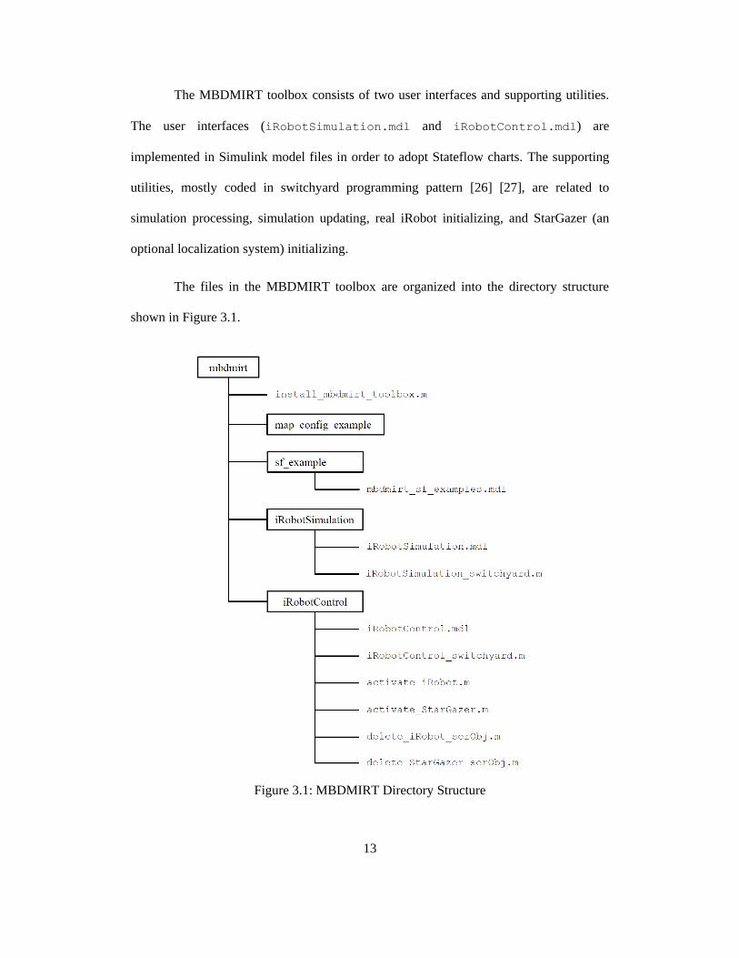
The files in the MBDMIRT toolbox are organized into the directory structure
shown in Figure 3.1.
Figure 3.1: MBDMIRT Directory Structure

14
The iRobotSimulation.mdl is the interface (shown in Figure 3.2) for
simulating multiple iRobots with Stateflow charts. It provides a Stateflow Chart Block
for end-users to design the control logic of the virtual iRobot Creates. In addition, it also
contains an iRobot Monitor Block that visualizes the simulation (shown in Figure 3.3).
The design process of the iRobotSimulation.mdl is described in Section 3.2.4. A
tutorial on using iRobotSimulation.mdl can be found in Section 3.4.
Figure 3.2: MBDMIRT iRobot Simulation Interface
Figure 3.3: Virtual iRobots in Simulation

15
The iRobotControl.mdl is the interface (shown in Figure 3.4) for controlling
multiple iRobots with the same Stateflow charts after verification by simulation. It
provides a Stateflow Chart Block to run the control logic for the actual iRobot Creates.
The design process of the iRobotControl.mdl is described in Section 3.2.5. A tutorial
on using iRobotControl.mdl can be found in Section 3.4.
Figure 3.4: MBDMIRT iRobot Control Interface
3.2 MBDMIRT Design Process
Since MBDMIRT toolbox has to provide functionalities of simulating virtual iRobots and
controlling physical iRobots, the MBDMIRT design process is divided up into two sub-
processes: the Development of MBDMIRT iRobot Simulation and the Development of
MBDMIRT iRobot Control.
The Development of MBDMIRT iRobot Simulation begins from modeling
iRobots and continues with two phases of Simulink-based simulator development. The
Development of MBDMIRT iRobot Control consists of interfacing Stateflow charts with
the MTIC toolbox, and interfacing Stateflow charts with the StarGazer indoor

16
localization systems. Figure 3.5 shows the development process of the MBDMIRT
toolbox.
Figure 3.5: Development Process of MBDMIRT Toolbox
3.2.1 iRobot Create Mathematical Model
The iRobot Create is a differentially-driven two-wheeled robot. The bottom view of the
iRobot is illustrated in Figure 3.6. For simplicity, the distance between the driven wheels
approximates to the diameter of the iRobot Create. The top view of the simplified iRobot
Create is shown in Figure 3.7.

17
Figure 3.6: Bottom View of iRobot Create
(image copied from iRobot Create Owner’s Guide)
Figure 3.7: Simplified iRobot Create Model (top view)
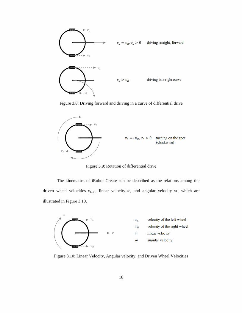
Bräunl [1] points out that ‘‘… driving control for differential drive is more
complex than for single wheel drive, because it requires the coordination of the two
driven wheels… If both motors run at the same speed, the robot drives straight forward or
backward, if one motor is running faster than the other, the robot drives in a curve along
the arc of a circle, and if both motors are run at the same speed in opposite directions, the
robot turns on the spot.’’ The above driving actions are illustrated in Figure 3.8 and
Figure 3.9.
18
Figure 3.8: Driving forward and driving in a curve of differential drive
Figure 3.9: Rotation of differential drive
The kinematics of iRobot Create can be described as the relations among the
driven wheel velocities , linear velocity , and angular velocity , which are
illustrated in Figure 3.10.
Figure 3.10: Linear Velocity, Angular velocity, and Driven Wheel Velocities

19
In order to model the kinematics of the iRobot Create, I start from Figure 3.11 to
determine the distance the iRobot has traveled, then discuss iRobot’s rotation angle
and derive kinematics of iRobot Create. The following derivation references Bräunl
[1] and Salzberger [16].
Assume a scenario in which the iRobot move along a circular segment, that is
illustrated in Figure 3.11.
Figure 3.11: Kinematics calculation for iRobot Create
Given the driven wheel velocities , the distances traveled by the driven
wheels can be derived by the following:
,
.
(3.1)

20
Thus, the distance the iRobot has traveled is:
(3.2)
Since is directional ( is negative if iRobot rotates clockwise, or
is positive if iRobot rotates counterclockwise), the analysis of can be broken into
two cases:
Case 1 ( , iRobot rotates clockwise):
Figure 3.12: iRobot's Rotation Angle while SR < SL
By observing Figure 3.12, we know:
(
) ,
(
) ,

21
and ,
,
,
.
Therefore, we know
(3.3)
Case 2 ( , iRobot rotates counterclockwise):
Figure 3.13: iRobot's Rotation Angle while SR > SL
By observing Figure 3.13, we know
(
) ,
(
) ,
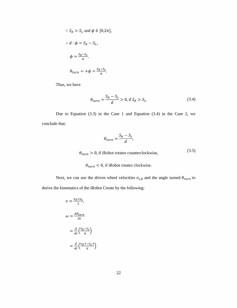
22
and ,
,
,
.
Thus, we have
(3.4)
Due to Equation (3.3) in the Case 1 and Equation (3.4) in the Case 2, we
conclude that:
if iRobot rotates counterclockwise,
if iRobot rotates clockwise.
(3.5)
Next, we can use the driven wheel velocities and the angle turned to
derive the kinematics of the iRobot Create by the following:
,
(
)
(
)

23
.
Thus, we know the kinematics of iRobot Create is:
(3.6)
Further, Equation (3.6) can be written into matrix form:
[
] [
],
[
] [
].
Thus, the kinematics of iRobot Create in matrix form is:
[
] [
] [
] (3.7)
Through Equation (3.6), we can also obtain the inverse kinematics of iRobot
Create:
,
,
,
,
,
24
[
],
[
].
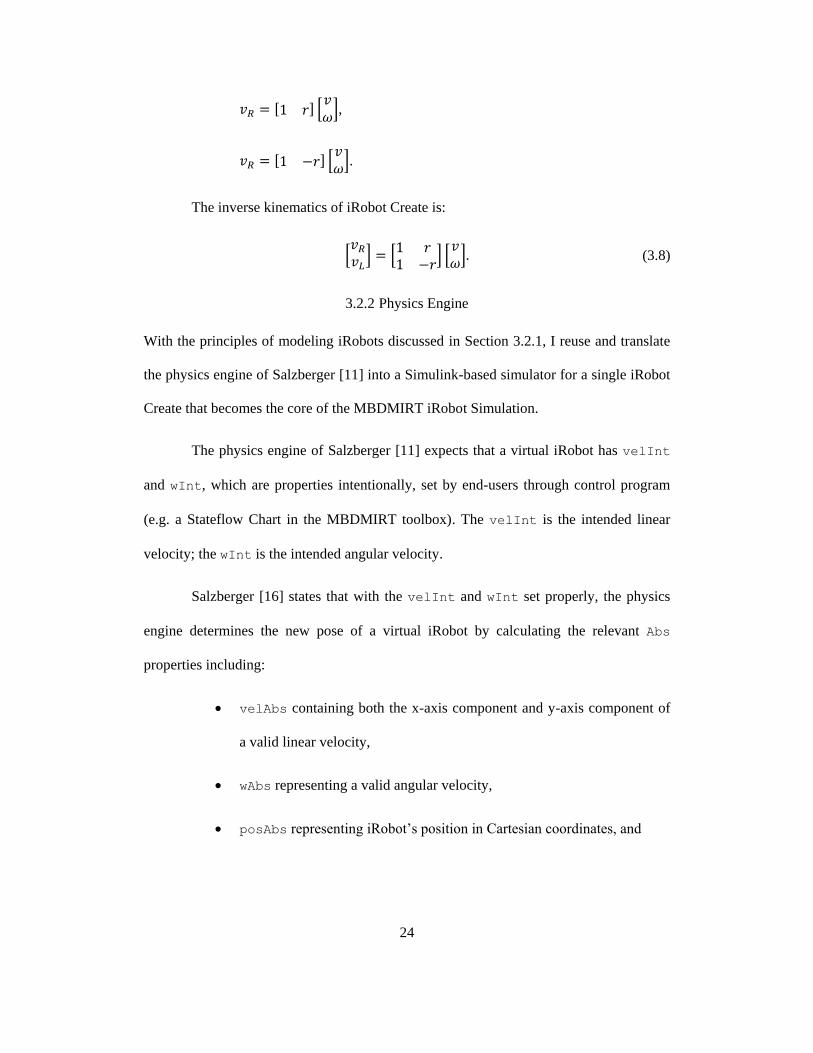
The inverse kinematics of iRobot Create is:
[
] [
] [
] (3.8)
3.2.2 Physics Engine
With the principles of modeling iRobots discussed in Section 3.2.1, I reuse and translate
the physics engine of Salzberger [11] into a Simulink-based simulator for a single iRobot
Create that becomes the core of the MBDMIRT iRobot Simulation.
The physics engine of Salzberger [11] expects that a virtual iRobot has velInt
and wInt, which are properties intentionally, set by end-users through control program
(e.g. a Stateflow Chart in the MBDMIRT toolbox). The velInt is the intended linear
velocity; the wInt is the intended angular velocity.
Salzberger [16] states that with the velInt and wInt set properly, the physics
engine determines the new pose of a virtual iRobot by calculating the relevant Abs
properties including:
velAbs containing both the x-axis component and y-axis component of
a valid linear velocity,
wAbs representing a valid angular velocity,
posAbs representing iRobot’s position in Cartesian coordinates, and

25
thAbs representing iRobot’s heading angle relative to the positive x-axis.
thAbs is wrapped to , which is the smaller angle relative to the
positive x-axis (the definition thAbs simplifies the sensor generating
function updateOdom explained in Section 3.2.3).
The physics engine updates the Abs properties by four physics engine functions,
including:
driveNormal: This function is called when the virtual iRobot is not
interacting with any walls.
drive1Wall: This function is called when one wall is affecting the
virtual iRobot.
drive2Wall: This function works similarly to drive1Wall but is
called when two walls are affecting the virtual iRobot.
driveCorner: This function operates when the virtual iRobot is
contacting the corner of one or two walls.
Salzberger [16] shows that each of the physics engine functions listed above
needs to be fed into that is the time since the last simulation update. Upon receiving
the , the physics engine uses the simple rule, , to caluculate the
virtual iRobot’s new position. is represented by tstep in the source code of both
Salzberger [11] and the MBDMIRT toolbox. For more details on the physics engine see
State Manipulator Functions (Physics Engine) in Salzberger [16].

26
3.2.3 Sensor Generating Functions
The new pose of a virtual iRobot is calculated by the physics engine. In the same manner,
the outputs of sensors on a virtual iRobot are processed by sensor generating functions
that are summarized in Table 3.1 and further explained in this section. The sensor
generating functions are translated from Salzberger [11].
Table 3.1: Sensor Generating Functions
Sensor Generating Function
iRobot’s
Built-in
Sensors
Bump Sensor genBump
Buttons (simulated by Button/LED Panel)
Cliff Sensor genCliff
Omni-Directional Infrared Receiver
(for iRobot Virtual Wall) genVWall
Odometer updateOdom
Wall Sensor genIR
Battery Meter –
Motor Current Meter –
Wheel Drop –
User-
Added
Sensors
Sonar genSonar
Light Detection And Ranging
(LIDAR) genLIDAR
Camera genCamera
Overhead Localization System genOverhead
Note: ‘–’ indicates unsupported sensor in the simulation.
genBump: The effective detection range of the virtual bump sensors is illustrated
in Figure 3.14. Most hits with the side ① or ③ will trigger the left or right bump sensors
respectively. Hits with side ② will trigger the front sensor. Note that the actual bump
sensors on a real iRobot Create may not be activated on a glancing blow. Whether the
real bump sensors are activated depends on the strength and the angle of the hit on an
object. For simplicity, these actual, physical effects are not taken into account by the
physics engine.

27
Figure 3.14: Detection Range of Virtual Bump Sensors
Button/LED Panel: There are Play (>) and Advance (>>|) button on the real
iRobot Create. The MBDMIRT toolbox represents these buttons in Button/LED Panel
accessible through the button in the upper right corner of the MBDMIRT simulation
visualization interface shown in Figure 3.3. The layout of the Button/LED Panel consists
of a set of one-touch buttons for all the iRobots and several sets of Buttons and LEDs for
a specific iRobot. The one-touch buttons can toggle all the Play buttons the Advance
buttons on the panel. The number of the button/LED set for a specific iRobot vary,
depending on how many virtual iRobots are currently being simulated. For example,
Figure 3.15 shows a panel for three virtual iRobots, and Figure 3.16 shows a panel for
seven virtual iRobots. Note that the buttons in the Button/LED Panel are toggle buttons,
which are activated by a push, and deactivated by another push. However, on the real
iRobot, the relevant MTIC instruction (ButtonSensorRoomba) will return true only if
the buttons are currently being held down.

28
Figure 3.15: Button/LED Panel for Three Virtual iRobots
Figure 3.16: Button/LED Panel for Seven Virtual iRobots
genCliff: The location of the virtual cliff sensors is illustrated in Figure 3.17.
Note that, in reality, the cliff sensors on a real iRobot check a single point on the ground,
while the point is on a real line that has thickness. However, the virtual lines on the map
for simulation have no thickness (see Appendix B for all the elements available on the
map for simulation). Thus, the effective detection point of the virtual cliff sensors are
increased to ranges that are different between the right (or left) cliff sensor and the front
right (or front left) cliff sensor. The right (or left) virtual cliff sensor is activated if a
virtual line intersects with the robot perimeter within 6.75°; the front right (or front left)

29
virtual cliff sensor is activated if a virtual line intersects with the robot perimeter within
5.85°. The effective detection ranges of the virtual cliff sensors are illustrated in Figure
3.18.
Figure 3.17: Location of Virtual Cliff Sensors
Figure 3.18: Detection Range of Virtual Cliff Sensors
genVWall: In reality, there is an omni-directional infrared receiver in front of a
real iRobot. One of the usages of the infrared receiver is to read signals from Virtual
Wall® (see page 14 of iRobot Corp. [10] for more information about Virtual Wall®). The
physics engine supports the simulation of the infrared receiver. A Virtual Wall® in reality
produces a field around the emitter and in the direction it faces, which is illustrated in
Figure 3.19. Similarly, a Virtual Wall® in MBDMIRT iRobot Simulation is represented

30
by a halo radius and effective signal range and angle, which is illustrated in Figure 3.20.
See Appendix B for how to set a Virtual Wall® on the map for simulation.
Figure 3.19: Invisible Barrier Created by Virtual Wall®
(image copied from iRobot Create Owner’s Guide)
Figure 3.20: Virtual Wall® in MBDMIRT iRobot Simulation
(revised image from MATLAB-Based Simulator for the iRobot Create
Code Documentation)
Salzberger [16] explains that ‘‘the physics engine checks whether a virtual
iRobot is against a Virtual Wall® by first comparing the sensor position to that of the
emitter to see if the iRobot is within the halo. If the iRobot is not in the halo, the physics
engine uses an area algorithm to see if the sensor position is inside the triangular field.

31
The area of a triangle is calculated from the vertices of the triangle using the determinant
method:
| (
)|.’’
Salzberger [16] explains further that ‘‘the physics engine calculates the area of
the triangular field, and then the area of the three triangles whose vertices are two vertices
from the field and the sensor position. If the sensor is within the field, then the area of the
field is equal to the sum of the areas of the other three triangles. If not, the area of the
three triangles is greater than the area of the field.’’
Figure 3.21: Determination of whether iRobot hits Virtual Wall®
(revised image from MATLAB-Based Simulator for the iRobot Create
Code Documentation)
updateOdom: This function is called at every execution of the simulation
updating function updateFigSim in the MBDMIRT toolbox (or the timer function
updateSim in Salzberger [11]). Salzberger [16] makes two assumptions regarding
updateOdom:

32
1. The movements of the virtual iRobot between two calls on updateOdom
is small,
2. The angle the virtual iRobot has turned between two calls on
updateOdom is small.
The first assumption simplifies the algorithm in calculating the odometry
distance. ‘‘The odometry distance is calculated by using a linear approximation of the
distance traveled between the previous location and the current one. The magnitude of the
change odomDist comes from a simple distance formula. The sign of the change is more
complicated. If the robot is moving in the direction it is pointing, the odometry will
increase, and vice-versa’’ (Salzberger [16], p. 28). The Figure 3.22 illustrates the
calculation of the odometry distance.
Figure 3.22: Sign of Odometry Distance
(revised image from MATLAB-Based Simulator for the iRobot Create
Code Documentation)

33
The second assumption regarding updateOdom simplifies the calculation of the
angular odometry. ‘‘The angle turned on a given step is calculated from the start thAbs,
and the end thAbs, with no knowledge of which path is taken. The path could be
determined from wAbs, but that would be more difficult than just assuming that the
iRobot turns the shorter amount. This is especially important when the robot turns
through or – radians, since thAbs is automatically wrapped to between those values.
In the diagram below, the odometry will be changed by the small angle of the two . It
will be increased if wAbs is positive, and decreased if negative.’’ If the maximum
allowable turning speed is large compared to the rate of updating the simulation, this
method may cause errors (Salzberger [16], p. 28).
Figure 3.23: Calculation of Angular Odometry
(revised image from MATLAB-Based Simulator for the iRobot Create
Code Documentation)
genIR: On the real iRobot Create, there is infrared proximity sensor with a very
low effective range on the front right of the bumper. The output of the sensor is a
Boolean value indicating whether a wall is detected. The counterpart on a virtual iRobot
locates at the position shown in Figure 3.24. The linear effective range is assumed within
0.1 meter from the location.

34
Figure 3.24: Location of Virtural Infrared Proximity Wall Sensor
In addition to the sensors built-in on the real iRobot Create, there are four user-
added sensors available in the simulation, including sonar sensors, LIDAR, a camera, and
an overhead localization system. A real overhead localization system (StarGazer indoor
localization system by Hagisonic, Inc.) is supported in the MBDMIRT iRobot Control.
See Section 3.2.5 for more information about StarGazer with the MBDMIRT toolbox.
genSonar: Salzberger [16] states that ‘‘… there are four sonar sensors, placed in
the cardinal directions on the edges of the robot. This makes it easy to check each sensor
since they are evenly spaced around the circumference.’’ Note the difference between the
order of outputs from genSonar and the sonar sensor actually called by
ReadSonarSpecified, which is a Stateflow graphical function in the MBDMIRT
iRobot Simulation:
The output of genSonar is a row vector with four elements, which is
[front left back right].
The syntax of the ReadSonarSpecified is
distance = ReadSonarSpecified(serPort, sonarNum). The
sonarNum must be an integer corresponding to sonar to be read, where:
1 represents the right virtual sonar, 2 – front, 3 – left, 4 – back.

35
genLidar: Salzberger [16] mentions that ‘‘… the LIDAR sensor is located on
the front of the robot… Like genSonar, this function calls findDist to get the reading
for each point in the LIDAR field of view.’’
genCamera: In Salzberger [17], it is mentioned that ‘‘… assumed a camera has
been installed on the front of the Create. This camera is to be used for color blob
detection only… The camera is used for finding beacons.’’ Beacons are a kind of
elements available on the map for simulation. They are immaterial objects (e.g. colored
paint or paper) on the ground, so the virtual iRobot can pass over them. See Appendix B
for more information about the elements on the map for simulation.
genOverhead: Salzberger [16] states that ‘‘… the overhead localization system
is assumed to be very accurate, so it outputs the exact location and orientation of the
robot with no noise.’’ In addition to the virtual overhead localization system, the
MBDMIRT iRobot Control supports a real localization system (StarGazer manufactured
by Hagisonic Inc.). See Appendix A for more information about the StarGazer.
3.2.4 Development of MBDMIRT iRobot Simulation
3.2.4.1 Simulink Graphical Animation
The MBDMIRT iRobot Simulation adopts Stateflow, which is an extension to Simulink,
for users to design the control logic of the virtual iRobots in the simulation. Thus, an
effective way to visualize the movements of the iRobots as Simulink animations is
required in the MBDMIRT toolbox, which leads the discussion in this section into
Simulink graphical animations.
Simulink graphical animation is an animation displaying the data received from a
Simulink model as the model executes. There are several approaches to developing

36
Simulink graphical animation, such as callback-based animation, S-Function-based
animation, the Animation Toolbox, the Dials & Gauges Blockset, and the Virtual Reality
Toolbox. These methods are discussed in Dabney [13] [28], where the Dials & Gauges
Blockset is obsolete and has been replaced by Gauges Blockset [29] [30]. Dabney [13]
[28] shows that the callback-based animation is the most powerful techniques compared
to other alternatives. By using the callback-based animation, Dabney [28] states that ‘‘...
it permits you to include custom controls in the animation window, and also allows you
to build an animation block that can be open or closed during a simulation.’’ Therefore,
the MBDMIRT iRobot Simulation is implemented with the callback-based animation.
3.2.4.2 Simulink Callback-Based Animation
The technique of Simulink callback-based animation is realized by use of the Simulink
callback parameters and an M-file function containing the callbacks written in switchyard
style. A template for Simulink callback-based animation is available in Debney [13].
The callback parameters associated with a Simulink block or with a Simulink
model contain MATLAB commands, such that when certain events (for example,
opening a model or double-clicking a block) occurs, the MATLAB commands are
executed. Listed in Table 3.2 is a portion of the callback parameters associated with a
particular Simulink block, courtesy of Dabney [13]. See The MATLAB, Inc. [31] for a
complete list of the callback parameters.
37
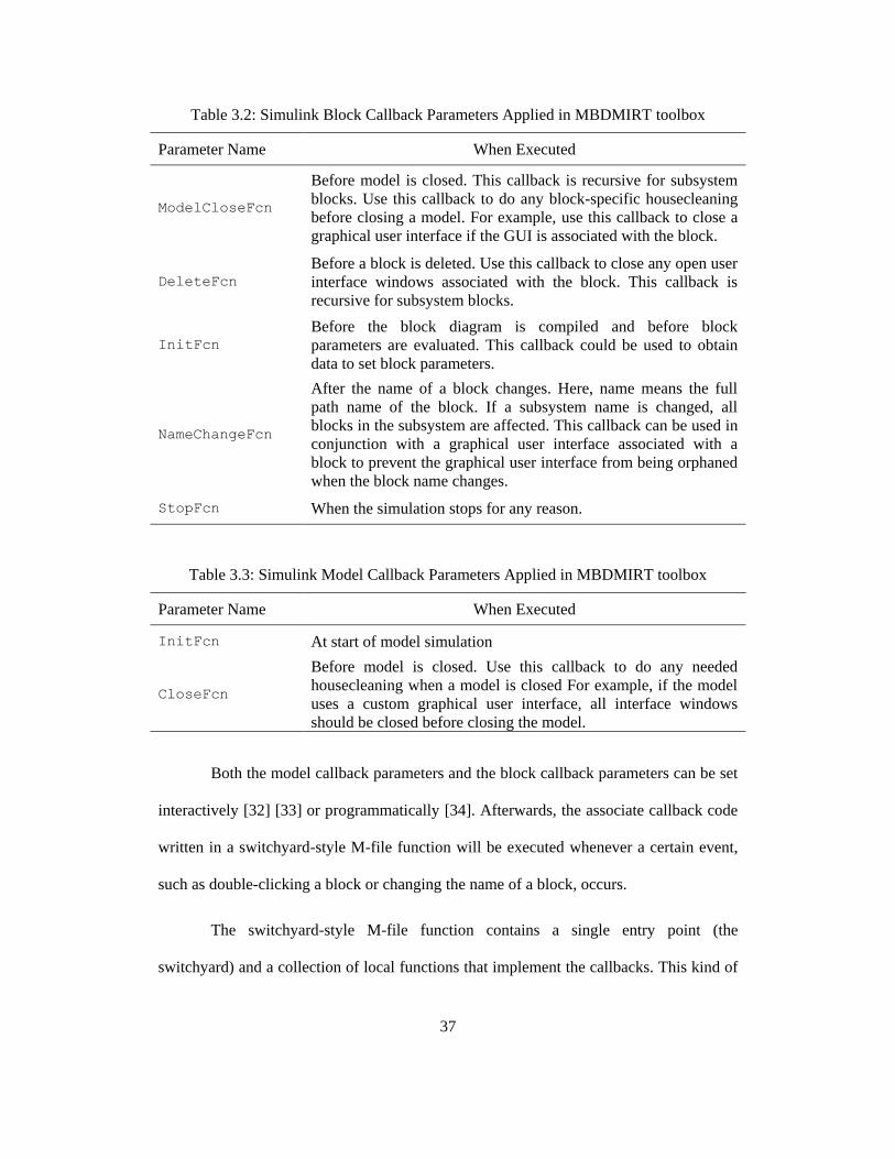
Table 3.2: Simulink Block Callback Parameters Applied in MBDMIRT toolbox
Parameter Name When Executed
ModelCloseFcn
Before model is closed. This callback is recursive for subsystem
blocks. Use this callback to do any block-specific housecleaning
before closing a model. For example, use this callback to close a
graphical user interface if the GUI is associated with the block.
DeleteFcn
Before a block is deleted. Use this callback to close any open user
interface windows associated with the block. This callback is
recursive for subsystem blocks.
InitFcn
Before the block diagram is compiled and before block
parameters are evaluated. This callback could be used to obtain
data to set block parameters.
NameChangeFcn
After the name of a block changes. Here, name means the full
path name of the block. If a subsystem name is changed, all
blocks in the subsystem are affected. This callback can be used in
conjunction with a graphical user interface associated with a
block to prevent the graphical user interface from being orphaned
when the block name changes.
StopFcn When the simulation stops for any reason.
Table 3.3: Simulink Model Callback Parameters Applied in MBDMIRT toolbox
Parameter Name When Executed
InitFcn At start of model simulation
CloseFcn
Before model is closed. Use this callback to do any needed
housecleaning when a model is closed For example, if the model
uses a custom graphical user interface, all interface windows
should be closed before closing the model.
Both the model callback parameters and the block callback parameters can be set
interactively [32] [33] or programmatically [34]. Afterwards, the associate callback code
written in a switchyard-style M-file function will be executed whenever a certain event,
such as double-clicking a block or changing the name of a block, occurs.
The switchyard-style M-file function contains a single entry point (the
switchyard) and a collection of local functions that implement the callbacks. This kind of

38
switchyard programming has several advantages. Firstly, it encapsulates all the callback
functions into a single M-file, such that the problem of M-file proliferation is eliminated
[26]. Secondly, ‘‘… because each callback function manipulates variables in its own
workspace, those variables are protected from changes made in the base workspace’’
(Webb [35]).
3.2.4.3 Review of Cornell’s MATLAB-Based Simulator in Autonomous Mode
When the MATLAB-based Simulator for the iRobot Create [11] is called, it initializes an
iRobot object and a timer object with a timer function updateSim. The iRobot object is
an instance of the user-defined class CreateRobot, which contains the properties of the
virtual iRobot, such as velInt, wInt, and the Abs properties. The task of the timer
object is to update the simulation every 0.1 second.
When the initialization process completes, the user can load a map and a
configuration file. Then, the simulator enters into the autonomous mode when the user
clicks the Autonomous Start button. Afterwards, the simulation begins and continues as
the control program executes. Meanwhile, the timer object will call updateSim to
update the visualization of the simulation every 0.1 second by interrupting the execution
of the control program. The simulation stops when the control program reaches the end of
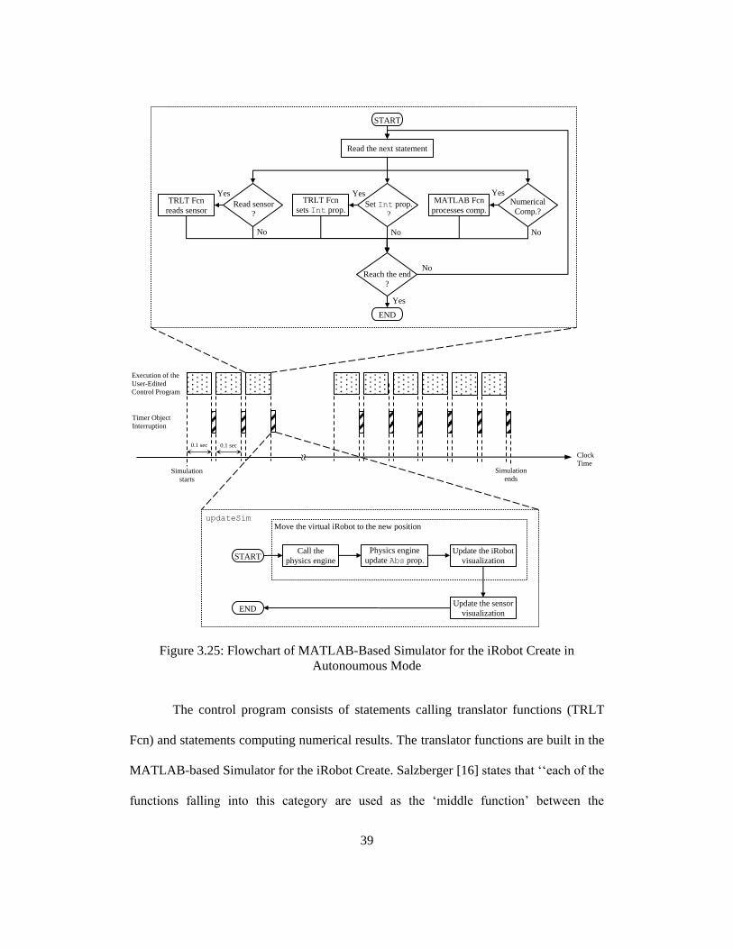
its code. The above description is shown diagrammatically in Figure 3.25.
39
Figure 3.25: Flowchart of MATLAB-Based Simulator for the iRobot Create in
Autonoumous Mode
The control program consists of statements calling translator functions (TRLT
Fcn) and statements computing numerical results. The translator functions are built in the
MATLAB-based Simulator for the iRobot Create. Salzberger [16] states that ‘‘each of the
functions falling into this category are used as the ‘middle function’ between the
0.1 sec
Execution of the
User-Edited
Control Program
Timer Object
Interruption 0.1 sec
Clock
Time
~ ~
Simulation
starts
Simulation
ends
START
END
Call the
physics engine Physics engine
update Abs prop. Update the iRobot
visualization
Update the sensor
visualization
Move the virtual iRobot to the new position
START
Read the next statement
Read sensor
? Set Int prop.
? Numerical
Comp.? TRLT Fcn
reads sensor
Reach the end
?
TRLT Fcn sets Int prop.
MATLAB Fcn
processes comp.
END
No
Yes
Yes Yes Yes
No No No
updateSim

40
autonomous control program and the simulator’s raw algorithms and data.’’ Therefore,
the control program can call the relevant translator functions to set intended velocity
velInt or read virtual sensor outputs. The character of the translator functions in
Cornell’s MATLAB-based simulator is illustrated in Figure 3.26.
Figure 3.26: Component Relationships of Cornell's MATLAB-Based Simulator in
Autonomous Mode
The main tasks of the timer object are to move the virtual iRobot to its new
position and update the sensor visualization. The timer object achieves these tasks by
interrupting the control program at a regular interval (every 0.1 sec in real clock time).
During the interruption, a timer function associated with the timer object invokes the
physics engine to compute iRobot’s new Abs properties. Next, the timer function uses the
new Abs properties to update the visualization of the iRobot and the virtual sensors.
3.2.4.4 Simulink Solver Type and Simulation Speed
The MBDMIRT iRobot Simulation is a Simulink-based simulator. Therefore, the
simulation speed depends on versatile factors such as Simulink model complexity,
Simulink solver step sizes, and the CPU speed. In order for the MBDMIRT iRobot
41
Simulation to have consistent performance such as the same simulation speed and the
same total simulation time on different PCs, a RealTime Pacer Block [36] is applied in
the MBDMIRT toolbox. The RealTime Pacer Block synchronizes the simulation time
with real elapsed time.
The Simulink environment provides a variety of solvers such as a fixed-step
solver and a variable-step solver. The main task of a solver is to determine the time of the
next simulation step. The MathWorks, Inc. [37] states that ‘‘both fixed-step and variable-
step solvers compute the next simulation time as the sum of the current simulation time
and a quantity known as the step size. With a fixed-step solver, the step size remains
constant throughout the simulation. In contrast, with a variable-step solver, the step size
can vary from step to step, depending on the model dynamics. In particular, a variable-
step solver increases or reduces the step size to meet the error tolerances that you
specify.’’ Moreover, ‘‘Simulation time is not the same as clock time. For example,
running a simulation for 10 seconds usually does not take 10 seconds. Total simulation
time depends on factors such as model complexity, solver step sizes, and computer
speed’’ (The MathWorks, Inc. [38]).
Consequently, the RealTime Pacer Block [36] is introduced in order for the
MBDMIRT iRobot Simulation to have consistent performance on different PCs. By
slowing down the simulation time, the RealTime Pacer Block synchronizes the
simulation with real elapsed clock time. However, Vallabha [36] mentions a technical
issue: ‘‘the matching between simulation time and elapsed time is approximate, with
expected difference on the order of 10 to 30 milliseconds. This limitation is due to
difficulties of precise timing with a multitasking operating system.’’

42
3.2.4.5 Translating Autonomous Mode of Cornell’s MATLAB-Based Simulator
into a Simulink-Based Simulator
The translation of Cornell’s MATLAB-based simulator into a Simulink-based simulator
for a single iRobot begins from the Simulink callback-based animation. The technique of
Simulation callback animation consists of a callback switchyard M-file and a Simulink
model file. The main components of the MATLAB-based simulator such as the physics
engine, the sensors generating functions (SENS GEN Fcn), the timer function
updateSim, and the translator functions (TRLT Fcn) are coded into the switchyard M-
file in the manner illustrated in Figure 3.27. The Simulink model file contains a Stateflow
Chart Block, a masked subsystem block, and a RealTime Pacer Block.
Figure 3.27: Translation of Cornell's MATLAB-Based Simulator
into a Simulink-Based Simulator
The Stateflow Chart Block in the Simulink-based simulator has a set of graphical
functions and a superstate named CPSLab. The supersate CPSLab is the place where
43
users can draw Stateflow charts to design their control logic for the virtual iRobot. The
users can call the graphical functions in their Stateflow chart to control the iRobot’s
behavior such as setting iRobot’s intended velocity or reading the virtual sensors.
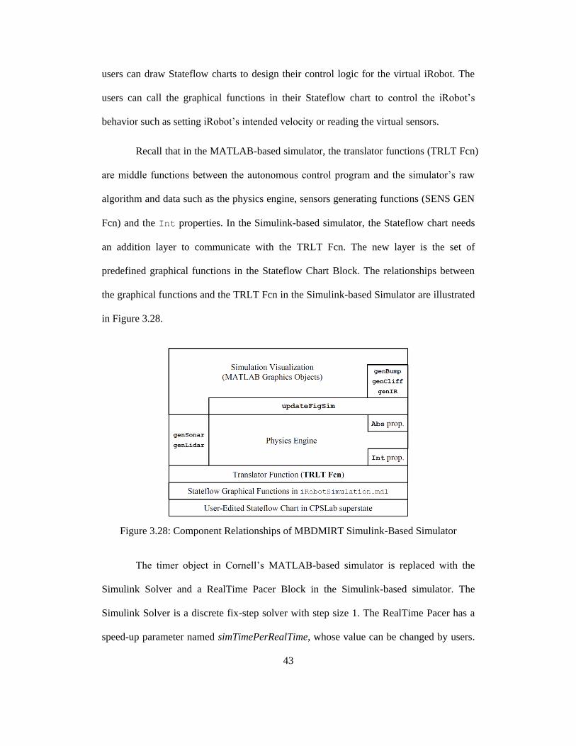
Recall that in the MATLAB-based simulator, the translator functions (TRLT Fcn)
are middle functions between the autonomous control program and the simulator’s raw
algorithm and data such as the physics engine, sensors generating functions (SENS GEN
Fcn) and the Int properties. In the Simulink-based simulator, the Stateflow chart needs
an addition layer to communicate with the TRLT Fcn. The new layer is the set of
predefined graphical functions in the Stateflow Chart Block. The relationships between
the graphical functions and the TRLT Fcn in the Simulink-based Simulator are illustrated
in Figure 3.28.
Figure 3.28: Component Relationships of MBDMIRT Simulink-Based Simulator
The timer object in Cornell’s MATLAB-based simulator is replaced with the
Simulink Solver and a RealTime Pacer Block in the Simulink-based simulator. The
Simulink Solver is a discrete fix-step solver with step size 1. The RealTime Pacer has a
speed-up parameter named simTimePerRealTime, whose value can be changed by users.

44
Since the Stateflow charts are invoked by the Simulink model in the way depicted in
Figure 3.29 [9], with the RealTime Pacer Block working with the discrete fix-step
Simulink Solver, the Stateflow charts will be invoked every
second in
real clock time, which means the physics engine and the updateFigSim will update the
simulation visualization every
second in real clock time. In fact, there
is a global variable named STperRT in the switchyard M-file, it stores the same value as
simTimePerRealTime. The physics engine is always fed into STperRT to compute the
iRobot’s new position according to the basic rule,
.
Therefore, the accuracy of the simulation is determined by
. The larger
the value of simTimePerRealTime is, the more accurate the iRobot simulation will be.
Figure 3.29: Stateflow charts are invoked in a cyclical manner
(image copied from Stateflow User’s Guide R2012a)
3.2.4.6 Expanding Simulation Capacity
The Simulink-based simulator introduced in Section 3.2.4.5 is able to simulate only a
single iRobot Create. In this section, the upgrades of the simulation capacity will be

45
introduced. The result is the MBDMIRT iRobot Simulation, which is a Simulink-based
Simulator capable of simulating multiple iRobots. Besides, the new simulator can read
the local PC clock, such that the virtual iRobots can make decisions based on time stamp
or the readings from the local clock.
The representation of both the virtual iRobot and walls in the Simulink-based
simulator are MATLAB lineseries graphics objects created by plot function.
Originally, the physics engine processes only the interactions among the iRobot graphics
object and the wall graphics objects. With the same physics engine, multiple virtual
iRobots goes through with each other when they collide. This is incorrect simulation
because the collision is not visualized. The solution is to create a view of obstacles for
every virtual iRobot. In an iRobot’s view, obstacles include all walls and other iRobot
graphics objects. Each iRobot’s view of obstacle is stored in mapObstacles, which is a
MATLAB matrix. Each row in mapObstacles represents a line object:
.
The whole mapObstacles contains the line objects representing all the wall
graphics objects and the other iRobot graphics objects from a specific iRobot’s view.
Each iRobot has its own mapObstacles (or its own view of obstacles). The drawback of
this solution is that every time the simulation visualization is updated by updateFigSim,
updateFigSim has to refresh every mapObstacles associated with each virtual
iRobots, which increases the computation burden.
Besides the multi-iRobot simulation, a new Stateflow graphical function,
LocalPCClock, reading local PC clock is also introduced into the new Simulink-based

46
simulator. Through the new graphical function, users can apply time stamps to their
Stateflow charts, such that the virtual iRobots behaves according to real clock time.
3.2.5 Development of MBDMIRT iRobot Control
The purpose of the MBDMIRT iRobot Control is for users to control real iRobot Creates
by executing, without modification, the control Stateflow charts designed in the
MBDMIRT iRobot Simulation. In addition, the MBDMIRT toolbox is designed to
support StarGazer indoor localization system, so the relevant facilities are introduced in
the MBDMIRT iRobot Control.
In order to execute the same Stateflow charts in the simulator and on the real
iRobots without modification, the MBDMIRT iRobot Control has a set of Stateflow
graphical functions with the same function signatures as those in the MBDMIRT iRobot
Simulation. The new set of Stateflow graphical functions are interface layer between the
MTIC toolbox and the user-created Stateflow charts. In the graphical functions, MTIC
commands are accessed through Stateflow ml function. For example, calling MTIC
command SetFwdVelAngVelCreate to set the forward velocity and angular velocity of
a real iRobot Create is achieved by the following command in the graphical functions,
where the serObjNum, FwdVel, AngVel are Stateflow data:
Similarly, calling MTIC commands AngleSensorRoomba to read angular
odometry on the real iRobot is achieved by the following command in the graphical
functions, where the AngleR and serObjNum are Stateflow data:
ml('SetFwdVelAngVelCreate(iRobot_%d, %f, %f)', serObjNum, FwdVel, AngVel)
AngleR = ml('AngleSensorRoomba(iRobot_%d)', serObjNum)
47
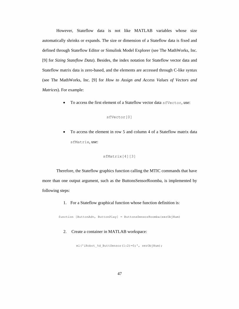
However, Stateflow data is not like MATLAB variables whose size
automatically shrinks or expands. The size or dimension of a Stateflow data is fixed and
defined through Stateflow Editor or Simulink Model Explorer (see The MathWorks, Inc.
[9] for Sizing Stateflow Data). Besides, the index notation for Stateflow vector data and
Stateflow matrix data is zero-based, and the elements are accessed through C-like syntax
(see The MathWorks, Inc. [9] for How to Assign and Access Values of Vectors and
Matrices). For example:
To access the first element of a Stateflow vector data sfVector, use:
To access the element in row 5 and column 4 of a Stateflow matrix data
sfMatrix, use:
Therefore, the Stateflow graphics function calling the MTIC commands that have
more than one output argument, such as the ButtonsSensorRoomba, is implemented by
following steps:
1. For a Stateflow graphical function whose function definition is:
2. Create a container in MATLAB workspace:
sfVector[0]
sfMatrix[4][3]
function [ButtonAdv, ButtonPlay] = ButtonsSensorRoomba(serObjNum)
ml('iRobot_%d_ButtSensor(1:2)=0;', serObjNum);
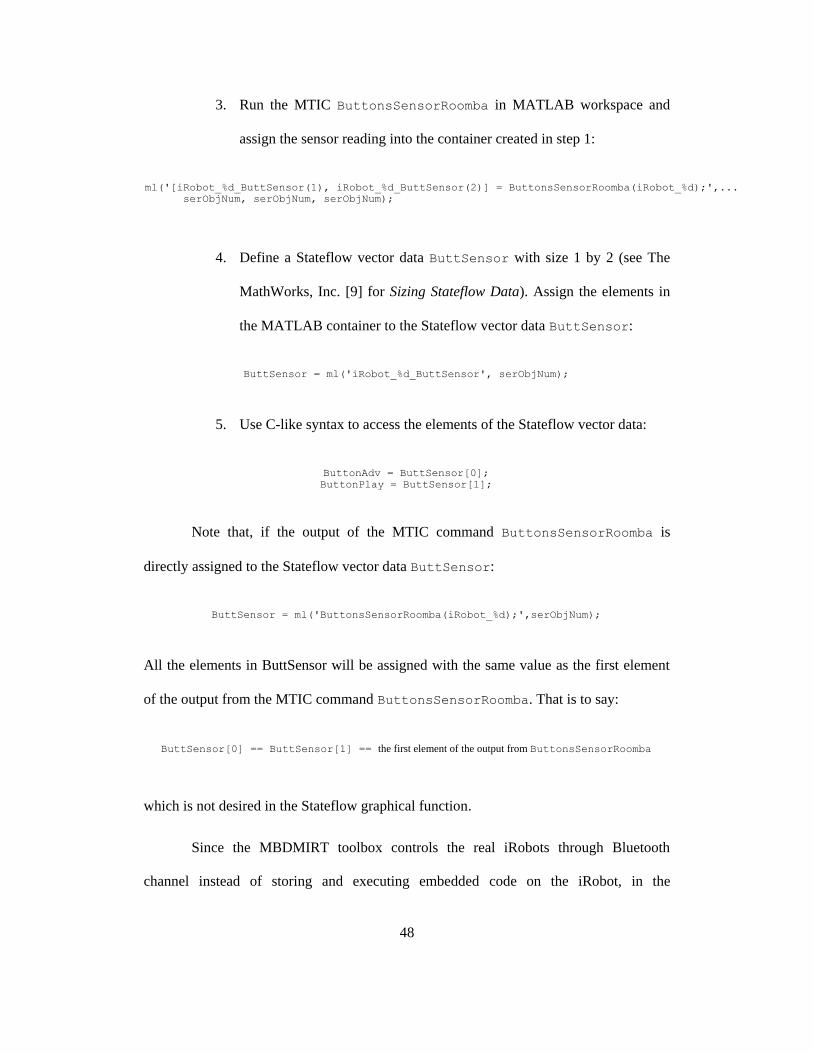
48
3. Run the MTIC ButtonsSensorRoomba in MATLAB workspace and
assign the sensor reading into the container created in step 1:
4. Define a Stateflow vector data ButtSensor with size 1 by 2 (see The
MathWorks, Inc. [9] for Sizing Stateflow Data). Assign the elements in
the MATLAB container to the Stateflow vector data ButtSensor:
5. Use C-like syntax to access the elements of the Stateflow vector data:
Note that, if the output of the MTIC command ButtonsSensorRoomba is
directly assigned to the Stateflow vector data ButtSensor:
All the elements in ButtSensor will be assigned with the same value as the first element
of the output from the MTIC command ButtonsSensorRoomba. That is to say:
which is not desired in the Stateflow graphical function.
Since the MBDMIRT toolbox controls the real iRobots through Bluetooth
channel instead of storing and executing embedded code on the iRobot, in the
ml('[iRobot_%d_ButtSensor(1), iRobot_%d_ButtSensor(2)] = ButtonsSensorRoomba(iRobot_%d);',...
serObjNum, serObjNum, serObjNum);
ButtSensor = ml('iRobot_%d_ButtSensor', serObjNum);
ButtonAdv = ButtSensor[0];
ButtonPlay = ButtSensor[1];
ButtSensor = ml('ButtonsSensorRoomba(iRobot_%d);',serObjNum);
ButtSensor[0] == ButtSensor[1] == the first element of the output from ButtonsSensorRoomba

49
MBDMIRT iRobot Control (iRobotControl.mdl) a RealTime Pacer Block works with
the Simulink discrete fixed-step solver in order to run the control Stateflow charts in real
time. The parameter simTimePerRealTime of the RealTime Pacer Block is set to 1000,
which is based on experiments. Thus, the communication rate between the control
Stateflow charts and the real iRobots is
.
The StarGazer localization system communicates with the MBDMIRT toolbox
through an adapter, which converts StarGazer’s RS-232 serial signal to Bluetooth radio
signal. The Stateflow graphical function OverheadLocalizationCreate, inspired by
the Cornell’s MATLAB-based simulator, reads the Bluetooth signals by calling the
supporting functions in iRobotControl_switchyard.m. Figure 3.30 shows the
system diagram of the MBDMIRT iRobot Control.
Figure 3.30: System Diagram of the MBDMIRT iRobot Control

50
3.3 Composition of the MBDMIRT Toolbox
The composition of the MBDMIRT toolbox is summarized in this section. The superstate
CPSLab, in other words, is a container of the control logic designed by end-users. The
control logic will drive both the virtual iRobots and the real iRobots via the mechanism
depicted in Figure 3.32 and Figure 3.33.
Figure 3.31: The CPSLab superstate is a container of control logic
Figure 3.32: Composition of MBDMIRT iRobot Simulation
Figure 3.33: Composition of MBDMIRT iRobot Control

51
3.4 MBDMIRT Tutorial
This tutorial assumes that the MBDMIRT toolbox is correctly installed (see Appendix A
for MBDMIRT installation instructions). We will go through a two-iRobot example in
which an iRobot moves along a line on ground, and the other iRobot will perform action
according to the local clock on the base station PC. The example begins from Stateflow
chart creation, iRobot simulation, and eventually to iRobot control.
Begin by typing
>> iRobotSimulation
at the MATLAB command prompt to invoke the iRobot Simulation interface shown in
Figure 3.2. Double-click the Stateflow Chart Block to enter the Stateflow Chart
workspace shown in Figure 3.34.
Figure 3.34: Stateflow Chart Workspace for MBDMIRT iRobot Simulation

52
Double-clicking the superstate CPSLab brings out the Stateflow Chart editor for
the simulation shown in Figure 3.35. The decomposition of the superstate CPSLab is
parallel.
Figure 3.35: Stateflow Chart Editor for MBDMIRT iRobot Simulation
Create two subcharted superstate. One is named iRobot_1; the other is named
iRobot_2 (as shown in Figure 3.36).
Figure 3.36: Containers of the Stateflow Charts for Two Virtual iRobots

53
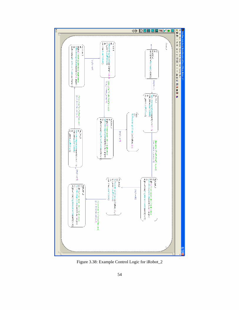
In the superstate iRobot_1, draw the Stateflow chart shown in Figure 3.37 and
add the relevant Stateflow data through Model Explorer or the Stateflow Editor. Similarly,
in the superstate iRobot_2, draw the Stateflow chart shown in Figure 3.38 and add the
relevant Stateflow data.
Figure 3.37: Example Control Logic for iRobot_1
54
Figure 3.38: Example Control Logic for iRobot_2

55
Go back to the iRobot Simulation interface, double-click the iRobot Monitor
Block. Then, a pop-up window shows up and inquires the quantity of the virtual iRobots
in the simulation. Enter ‘‘2’’ for this tutorial.
Figure 3.39: Pop-up Window inquiring iRobot Quantity
Clicking the OK button brings out the simulation monitor shown in Figure 3.40.
Figure 3.40: iRobot Simulation Monitor
Loading an pre-edited example map either through the Setup menu at the upper-
left corner the monitor, or through a keyboard shortcut Ctrl+M. Either way bring up a
folder window for you to choose a desired map. In this tutorial, we choose the example
map. Loading the map refreshes the monitor, which is shown in Figure 3.41.

56
Figure 3.41: iRobot Simulation Monitor with a Loaded Map
Next, set up the origin position for the virtual iRobots either through the Setup
menu at the upper-left corner the monitor, or through a keyboard shortcut Ctrl+R. Set the
origin positions the same as those shown in Figure 3.42.
Figure 3.42: Origin Positions of the iRobots
Go back to the iRobot Simulation interface, starting the simulation makes the
iRobot_1 moves along the line on ground, and the iRobot_2 to make a right turn
approximately every 5 second in real clock time.

57
After verification by simulation, we can execute the same Stateflow charts to
control real iRobots. Begin by typing
>> iRobotControl
at the MATLAB command prompt to invoke the iRobot Control interface shown in
Figure 3.4.
In the same manner, double-click the Stateflow Chart Block and go into the
superstate CPSLab in the iRobot Control Interface. Then, copy the Stateflow Charts
designed in the simulation stages into the superstate CPSLab of the control interface.
Next, prepare two real iRobot, mark one of them as iRobot_1, the other as
iRobot_2. Connect the Bluetooth Adapter Modules (BAMs) to the iRobots. Power up the
iRobots. Assume the BAM on iRobot_1 has been assigned with COM 5 to communicate
with the base station PC, and the BAM on iRobot_2 with COM 6 (see Element Direct,
Inc. [19] for BAM installation instructions).
Before start running the Stateflow charts in the MBDMIRT iRobot Control
interface, we need to associate each BAM with corresponding iRobots. Now, the BAM
with COM 5 is installed on the iRobot_1, and the BAM with COM 6 is installed on the
iRobot_2. With the above information, typing
>> activate_iRobot(1, 5)
>> activate_iRobot(2, 6)
at the MATLAB command prompt. By doing so, the ideal numbers of each iRobot, such
as number 1 for the iRobot_1 and number 2 for the iRobot_2, are bound with correct
BAM. Thus, the same Stateflow charts design at the simulation stage can execute on the
real iRobots without any modification.

58
The execution of the function activate_iRobot for each real iRobot may take
1 to 2 minutes. After activating each iRobots, go back to the iRobot Control Interface,
start the simulation of the Simulink model. This time, instead of the virtual iRobots in the
simulation monitor, the real iRobot Creates will move in the same manner as in the
simulation monitor, which completes this tutorial.

59
CHAPTER 4
RESULTS AND FUTURE WORK
In this thesis, the development and structure of the MBDMIRT toolbox is described. The
main contribution of this thesis is:
The MBDMIRT toolbox as an enhancement to MATLAB & Simulink, such
that Simulink/Stateflow is linked to both a multi-iRobot simulator interface and
a multi-iRobot control interface.
The toolbox was designed to help users acquire and practice the Model-Based
Development skills necessary to design real-time embedded system. Through
the toolbox, this goal is achieved by:
1. Using Stateflow charts to design control logic for virtual iRobots,
2. Running the simulator to check the correctness of the Stateflow charts,
3. After verification by simulation, running the same Stateflow chart
without modification to control real iRobots.
MBDMIRT toolbox was designed to run in real clock time. To enable this
functionality, a RealTime Pacer Block is introduced to work with Simulink
Solver.
4.1 Future Work
From many viewpoints, the MBDMIRT toolbox could be improved with numerous ways.
A few of these are mentioned below:

60
Conduct surveys on users’ experience. The effectiveness of the MBDMIRT
toolbox in MBD education could be evaluated by surveying its users. The
evaluation will be important in updating the toolbox functionalities.
Generate real-time embedded code from the verified Stateflow charts. Instead
of controlling iRobots from a host PC, running real-time embedded code on the
iRobots provides more efficient and accurate control. A candidate controller
able to execute code on the real iRobot is the iRobot Command Module [10]
[39]. One of the concerns about it is that the Command Module has only
general purposes I/O (GPIO). Thus, it could be difficult to let devices with RS-
232 serial port communicate with the Command Module.
This thesis introduces and demonstrates the MBDMIRT toolbox. There are still
numerous ways in which the MBDMIRT toolbox could be revised. I hope it will
eventually contribute the education of Model-Based Development in ways I never
imagined.

61
REFERENCES
[1] R. Baheti and H. Gill, "Cyber-physical Systems," IEEE Control Systems Society,
2011.
[2] A. Sangiovanni-Vincentelli and M. Di Natale, "Embedded System Design for
Automotive Applications," Computer, vol. 40, no. 10, pp. 42-51, 2007.
[3] T. A. Henzinger and J. Sifakis, The Embedded Systems Design Challenge, vol.
4085/2006, J. Misra, T. Nipkow and E. Sekerinski, Eds., Heidelberg, Berlin:
Springer-Verlag, 2006, pp. 1-15.
[4] P. Liggesmeyer and M. Trapp, "Trends in Embedded Software Engineering,"
IEEE Software, vol. 26, no. 3, pp. 19-25, 2009.
[5] E. A. Lee and S. A. Seshia, "The Design Process," in Introduction to Embedded
Systems: A Cyber-Physical Systems Approach, LeeSeshia.org, 2011, pp. 8-15.
[6] J. C. Jensen, "Elements of Model-Based Design," University of California,
Berkeley, Technical Memorandum. UCB/EECS-2010-19, February 2010.
[7] D. Harel, "Statecharts: A Visual Formalism for Complex Systems," Science of
Computer Programming, vol. 8, pp. 231-274, 1987.
[8] D. Harel, "Statecharts in the making: a personal account," Communications of the
ACM, vol. 52, no. 3, pp. 67-75, March 2009.
[9] The MathWorks, Inc., "Stateflow® User’s Guide R2012a," March 2012. [Online].
Available: http://www.mathworks.com/help/pdf_doc/stateflow/sf_ug.pdf.
[Accessed 12 October 2012].
[10] iRobot Corporation, "iRobot® Create Owner’s Guide," 2006. [Online]. Available:
http://www.irobot.com/filelibrary/create/create%20manual_final.pdf. [Accessed
18 September 2012].
[11] C. Salzberger, H. Kress-Gazit and K.-Y. D. Fan, "MATLAB-based Simulator for
the iRobot Create," 2011. [Online]. Available:
http://web.mae.cornell.edu/hadaskg/CreateMATLABsimulator/createsimulator.ht
ml.
[12] D. Hanselman and B. Littlefield, "Graphical User Interface," in Mastering
MATLAB 7, Upper Saddle River, New Jersey: Pearson Education Inc., 2005, pp.
539-570.
[13] J. B. Dabney and T. L. Harman, "Callback-Based Animations," in Mastering
Simulink, Upper Saddle River, New Jersey: Pearson Education Inc., 2004, pp.
215-218.

62
[14] J. M. Esposito, O. Barton and J. Kohler, "MATLAB Toolbox for the iRobot
Create," 2011. [Online]. Available:
www.usna.edu/Users/weapsys/esposito/roomba.matlab/.
[15] K.-Y. D. Fan and K. C. Dimiduk, "Using the Matlab-based iRobot Create
Simulator to Engage Introductory Computer Programming Students in Program
Development and Observing Computational Errors," in Frontiers in Education
Conference, Rapid City, 2011.
[16] C. Salzberger, H. Kress-Gazit and K.-Y. D. Fan, "MATLAB Simulator for the
iRobot Create Code Documentation," 1 February 2011. [Online]. Available:
http://web.mae.cornell.edu/hadaskg/CreateMATLABsimulator/Code%20Docume
ntation.pdf. [Accessed 15 October 2012].
[17] C. Salzberger, H. Kress-Gazit and K.-Y. D. Fan, "MATLAB Simulator for the
iRobot Create User Manual," 1 February 2011. [Online]. Available:
http://web.mae.cornell.edu/hadaskg/CreateMATLABsimulator/Code%20Docume
ntation.pdf. [Accessed 15 October 2012].
[18] iRobot Corporation, "iRobot® Create OPEN INTERFACE," 2006. [Online].
Available:
http://www.irobot.com/filelibrary/pdfs/hrd/create/create%20open%20interface_v2
.pdf. [Accessed 13 October 2012].
[19] Element Direct, Inc., "BAM for the iRobot® Create™ Owner's Manual," 16 July
2007. [Online]. Available: http://www.elementdirect.com/files/10542B.pdf.
[Accessed 13 October 2012].
[20] J. C. Jensen, "Model-Based Design With the NI Robotics Simulator and the
iRobot Create," 11 August 2011. [Online]. Available:
https://decibel.ni.com/content/docs/DOC-17597. [Accessed 14 October 2012].
[21] National Instruments Corporation, "NIWeek 2011 Conference Program," 2011.
[Online]. Available:
http://www.ni.com/pdf/niweek/us/2011/NIWeek_2011_Conference_Program.pdf.
[Accessed 14 October 2012].
[22] J. C. Jensen, "A model-based design methodology for cyber-physical systems," in
Wireless Communications and Mobile Computing Conference (IWCMC), 2011
7th International, Istanbul, 2011.
[23] X. Hu and B. P. Zeigler, "A simulation-based virtual environment to study
cooperative robotic systems," Integrated Computer-Aided Engineering, vol. 12,
no. 4, pp. 353-367, 2005.
[24] Esterel Technologies, Inc., "SCADE Suite®," Esterel Technologies, Inc., 2012.
[Online]. Available: http://www.esterel-technologies.com/products/scade-suite/.
[Accessed 18 October 2012].
63
[25] National Instruments Corporation, "NI LabVIEW," National Instruments
Corporation, 2012. [Online]. Available: http://www.ni.com/labview/. [Accessed
18 October 2012].
[26] L. Shure, "Programming Patterns in MATLAB," The MathWorks, Inc., 17 June
2003. [Online]. Available:
http://www.mathworks.com/matlabcentral/fileexchange/3610-programming-
patterns-in-matlab. [Accessed 19 October 2012].
[27] D. Hanselman and B. Littlefield, "Callback Programming," in Mastering
MATLAB 7, Upper Saddle River, New Jersey: Pearson Education Inc., 2005, pp.
550-559.
[28] J. B. Dabney and T. L. Harman, "Graphical Animations," in Mastering Simulink,
Upper Saddle River, New Jersey: Pearson Education Inc., 2004, pp. 259-272.
[29] The MathWorks, Inc., "Gauges Blockset - Simulink," The MathWorks, Inc.,
2012. [Online]. Available: http://www.mathworks.com/products/gauges/.
[30] Matt and P. Goddard, "Where can I get the "dials & gauges bl... - Newsreader -
MATLAB Central," The MathWorks, Inc., 4 June 2012. [Online]. Available:
http://www.mathworks.com/matlabcentral/newsreader/view_thread/320710.
[31] The MathWorks, Inc., "Callback Functions - MATLAB & Simulink," The
MathWorks, Inc., 2012. [Online]. Available:
http://www.mathworks.com/help/simulink/ug/using-callback-functions.html.
[32] The MathWorks, Inc., "Specifying Callbacks," The MathWorks, Inc., 2012.
[Online]. Available: http://www.mathworks.com/help/simulink/ug/managing-
model-versions.html#f4-140344.
[33] The MathWorks, Inc., "Create Block Callback Functions," The MathWorks, Inc.,
2012. [Online]. Available: http://www.mathworks.com/help/simulink/ug/using-
callback-functions.html#f4-45560.
[34] The MathWorks, Inc., "Set Simulink system and block parameter value," The
MathWorks, Inc., 2012. [Online]. Available:
http://www.mathworks.com/help/simulink/slref/set_param.html.
[35] P. Webb, "GUI switchyards," The MathWorks, Inc., 2012. [Online]. Available:
http://www.mathworks.com/company/newsletters/news_notes/win00/prog_patter
ns.html. [Accessed 27 October 2012].
[36] G. Vallabha, "Real-Time Pacer for Simulink," The MathWorks, Inc., 21 October
2010. [Online]. Available:
http://www.mathworks.com/matlabcentral/fileexchange/29107-real-time-pacer-
for-simulink. [Accessed 28 October 2012].
64
[37] The MathWorks, Inc., "Simulink® User’s Guide R2012b," September 2012.
[Online]. Available:
http://www.mathworks.com/help/pdf_doc/simulink/sl_using.pdf. [Accessed 28
October 2012].
[38] The MathWorks, Inc., "Solver Pane - MATLAB & Simulink," The MathWorks,
Inc., 2012. [Online]. Available:
http://www.mathworks.com/help/simulink/gui/solver-pane.html. [Accessed 28
October 2012].
[39] iRobot Corporation, "iRobot® Command Module Owners manual," 2007.
[Online]. Available:
http://www.irobot.com/filelibrary/pdfs/hrd/create/Command%20Module%20Man
ual_v2.pdf. [Accessed 30 October 2012].

65
APPENDIX A
INSTALLING AND CONFIGURING THE MBDMIRT TOOLBOX

66
A.1 License Agreement
The MBDMIRT toolbox modifies the source code of the MATLAB-Based Simulator for
the iRobot Create by Cameron Salzberger. The MBDMIRT toolbox is written by Shih-
Kai Su, and its code is released under the open-source BSD license. A copy of the license
is provided with the software and listed below:
Copyright (c) 2012, Arizona State University
All rights reserved.
Redistributions of source code must retain the above copyright notice, this list of
conditions and the following disclaimer.
Redistributions in binary form must reproduce the above copyright notice, this list
of conditions and the following disclaimer in the documentation and/or other
materials provided with the distribution.
THIS SOFTWARE IS PROVIDED BY THE COPYRIGHT HOLDERS AND
CONTRIBUTORS "AS IS" AND ANY EXPRESS OR IMPLIED WARRANTIES,
INCLUDING, BUT NOT LIMITED TO, THE IMPLIED WARRANTIES OF
MERCHANTABILITY AND FITNESS FOR A PARTICULAR PURPOSE ARE
DISCLAIMED. IN NO EVENT SHALL THE COPYRIGHT OWNER OR
CONTRIBUTORS BE LIABLE FOR ANY DIRECT, INDIRECT, INCIDENTAL,
SPECIAL, EXEMPLARY, OR CONSEQUENTIAL DAMAGES (INCLUDING, BUT
NOT LIMITED TO, PROCUREMENT OF SUBSTITUTE GOODS OR SERVICES;
LOSS OF USE, DATA, OR PROFITS; OR BUSINESS INTERRUPTION) HOWEVER
CAUSED AND ON ANY THEORY OF LIABILITY, WHETHER IN CONTRACT,

67
STRICT LIABILITY, OR TORT (INCLUDING NEGLIGENCE OR OTHERWISE)
ARISING IN ANY WAY OUT OF THE USE OF THIS SOFTWARE, EVEN IF
ADVISED OF THE POSSIBILITY OF SUCH DAMAGE.
The views and conclusions contained in the software and documentation are those of the
authors and should not be interpreted as representing official policies, either expressed or
implied, of Arizona State University.
The iRobot simulator and graphical user interface contained within MBDMIRT were
modified from the iRobot Create Simulator Toolbox version 1.3 by Cornell University.
Copyright 2010 Cornell University. All rights reserved.
Redistribution and use in source and binary forms, with or without modification, are
permitted provided that the following conditions are met:
1. Redistributions of source code must retain the above copyright notice,
this list of conditions and the following disclaimer.
2. Redistributions in binary form must reproduce the above copyright
notice, this list of conditions and the following disclaimer in the
documentation and/or other materials provided with the distribution.
THIS SOFTWARE IS PROVIDED BY CORNELL UNIVERSITY "AS IS" AND ANY
EXPRESS OR IMPLIED WARRANTIES, INCLUDING, BUT NOT LIMITED TO,
THE IMPLIED WARRANTIES OF MERCHANTABILITY AND FITNESS FOR A
PARTICULAR PURPOSE ARE DISCLAIMED. IN NO EVENT SHALL CORNELL
UNIVERSITY OR CONTRIBUTORS BE LIABLE FOR ANY DIRECT, INDIRECT,
INCIDENTAL, SPECIAL, EXEMPLARY, OR CONSEQUENTIAL DAMAGES
(INCLUDING, BUT NOT LIMITED TO, PROCUREMENT OF SUBSTITUTE
68
GOODS OR SERVICES; LOSS OF USE, DATA, OR PROFITS; OR BUSINESS
INTERRUPTION) HOWEVER CAUSED AND ON ANY THEORY OF LIABILITY,
WHETHER IN CONTRACT, STRICT LIABILITY, OR TORT (INCLUDING
NEGLIGENCE OR OTHERWISE) ARISING IN ANY WAY OUT OF THE USE OF
THIS SOFTWARE, EVEN IF ADVISED OF THE POSSIBILITY OF SUCH DAMAGE.
The views and conclusions contained in the software and documentation are those of the
authors and should not be interpreted as representing official policies, either expressed or
implied, of Cornell University.
A.2 Required Hardware and Software for the MBDMIRT Toolbox
This section details the required hardware and software for the MBDMIRT toolbox. The
required software includes:
MATLAB & Simulink 2010b (or newer): The MBDMIRT toolbox was
developed on MATLAB 2012a, and has been tested on MATLAB 2010b.
It should work on all newer versions of MATLAB including Simulink
environment,
RealTime Pacer Block: It is obtainable through the link in The
MathWorks, Inc. [36]. For information about RealTime Pacer Block in
the MBDMIRT toolbox, see Section 3.2.4.4 and Section 3.2.5.
The required hardware includes:
iRobot Create: It is a differentially-driven two-wheeled ground vehicle.
For more information about iRobot Create, see the introduction at
http://www.irobot.com/us/robots/Educators/Create.aspx,

69
BAM: BAM is short for Bluetooth Adapter Module. It is used to connect
a control computer wirelessly to the iRobot Create. For more information
about BAM, see the introduction at http://www.elementdirect.com.
A.3 Optional Hardware for the MBDMIRT Toolbox
This section details the optional hardware for the MBDMIRT toolbox. The optional
hardware includes:
iRobot Virtual Wall: A Virtual Wall emits an adjustable infrared beam (8
feet in maximum) that the iRobot is able to detect. A Virtual Wall
prevents the iRobot from entering a specific area. For more information
about iRobot Virtual Wall, see http://www.irobot.com/us,
StarGazer Indoor Localization System: StarGazer outputs the current
Cartesian coordinates with respect to a StarGazer landmark. StarGazer
can be mounted on the iRobot Create to do guidance control based on the
coordinates. For more information about StarGazer, see http://
www.hagisonic.com/,
SIIG RS-232 Serial to Bluetooth Adapter: It is used to connect a control
computer wirelessly to the StarGazer. For more information about the
RS-232 Serial to Bluetooth Adapter, see http://www.siig.com/rs-232-
serial-to-bluetooth-adapter.html.
A.4 Installing the MBDMIRT Toolbox
1. Unzip the mbdmirt.zip
2. Copy the /mbdmirt folder to the path you desired. For example,
C:/userfolder/

70
3. Go to MATLAB, change MATLAB Current Folder to the path
C:/userfolder/mbdmirt
4. At MATLAB command prompt (>>), type and enter
>> install_mbdmirt_toolbox
5. After the function install_mbdmirt_toolbox completes execution,
the mbdmirt directory is added into and saved in the MATLAB path.

71
APPENDIX B
CREATION OF THE MAP FOR SIMULATION

72
The physics engine of the MBDMIRT iRobot Simulation is based on that of the Cornell’s
MATLAB-Based Simulator for the iRobot Create. Therefore, the MBDMIRT uses the
same map format for simulation. This appendix shows the types of elements available in
the map and the methods of creating a map, courtesy of the Cornell University’s user
manual [17].
B.1 Elements of the Map
There are four types of elements available in a map, including:
1. Walls: Represented by solid lines. The virtual iRobots are unable to pass
through them. Walls can trigger bump sensors, infrared proximity wall
sensor, sonar, and LIDAR.
2. Lines: Represented by dashed lines. Lines are used to indicate markings
on the ground, such as paints or tapes. The virtual iRobots can pass over
lines. Lines can change the readings of the cliff sensor signal strength
despite that there is no cliff in a map for simulation.
3. Beacons: Represented by colored circles. Beacons are used to indicate
some kinds of objects on the ground, such as colorful paints or papers.
The virtual iRobots can pass over them. Beacons are detectable only by
the camera.
4. Virtual Walls: Represented by a green asterisk and green lines showing
the range of the field. The virtual iRobots can pass through them. Virtual
Walls can trigger the omni-directional infrared sensor.
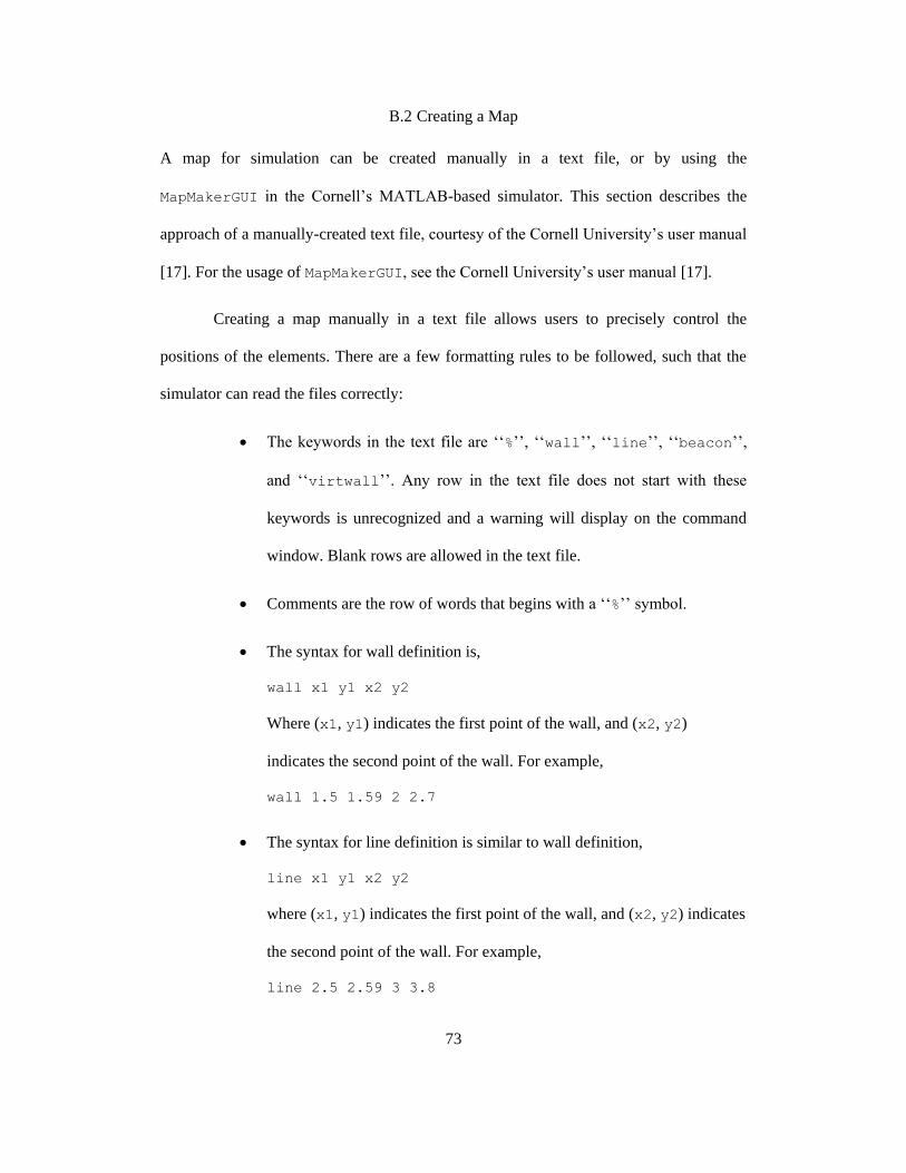
73
B.2 Creating a Map
A map for simulation can be created manually in a text file, or by using the
MapMakerGUI in the Cornell’s MATLAB-based simulator. This section describes the
approach of a manually-created text file, courtesy of the Cornell University’s user manual
[17]. For the usage of MapMakerGUI, see the Cornell University’s user manual [17].
Creating a map manually in a text file allows users to precisely control the
positions of the elements. There are a few formatting rules to be followed, such that the
simulator can read the files correctly:
The keywords in the text file are ‘‘%’’, ‘‘wall’’, ‘‘line’’, ‘‘beacon’’,
and ‘‘virtwall’’. Any row in the text file does not start with these
keywords is unrecognized and a warning will display on the command
window. Blank rows are allowed in the text file.
Comments are the row of words that begins with a ‘‘%’’ symbol.
The syntax for wall definition is,
wall x1 y1 x2 y2
Where (x1, y1) indicates the first point of the wall, and (x2, y2)
indicates the second point of the wall. For example,
wall 1.5 1.59 2 2.7
The syntax for line definition is similar to wall definition,
line x1 y1 x2 y2
where (x1, y1) indicates the first point of the wall, and (x2, y2) indicates
the second point of the wall. For example,
line 2.5 2.59 3 3.8

74
The syntax for beacon definition is,
beacon x y [r g b] id
where (x, y) indicates the Cartesian coordinates of the beacon, [r g b]
is the color vector of the beacon, and id is the beacon’s ID number
defined by user. For example,
beacon 1.5 -1.7 [0 1 0.5] 1
The syntax for Virtual Wall definition is,
virtwall x y th r
where (x, y) indicates the Cartesian coordinates of the emitter; th is the
angle (in radians) of the direction of emission relative to the positive x-
axis; r indicates the range setting (1 is the lowest range, 3 is the highest).
For example,
virtwall 2.5 3.3 -1.5 2

75
APPENDIX C
CREATION OF THE CONFIGURATION FILE FOR SIMULATION

76
A configuration file defines the properties of the virtual sensors in the simulation, such as
communication delay and noise. The physics engine of the MBDMIRT iRobot
Simulation is based on that of the Cornell’s MATLAB-Based Simulator for the iRobot
Create. Therefore, the MBDMIRT uses the same configuration file for simulation. This
appendix shows the types of elements available in the configuration and the methods of
creating a configuration, courtesy of the Cornell University’s user manual [17].
C.1 Elements of the Configuration
Communication Delay: Determines the response time for the iRobots.
Increasing this value causes longer delay for all commands, such as
setting velocity or reading sensor outputs, to the iRobots.
Noise Data: Noise data consists of mean and standard deviation. They
determine the fluctuation in the virtual sensors outputs. Noise data has
different meanings for each kind of virtual sensors, which is explained
below:
1. Wall sensor: The default effective range of the virtual wall sensor is
defined by a property rangeIR in the source code. The noise data changes
the effective range. The mean of the noise causes an offset from the
default range. The standard deviation causes the variance in the effective
range.
2. Cliff sensors: With no noise, the cliff sensor signal strengths will read
1.5% when over a line, and 21.5% when not. The real values of the
readings will vary based on room lighting, floor color and material, and
the sensors themselves. If real sensors tend to read higher or lower, set a

77
value in the noise mean that will change the sensor output. The standard
deviation adds to the variance in the readings.
3. Odometry: The odometry noise parameters should be given as a
percentage of the true measurement. For example, if the Stateflow
graphical function DistanceSensorRoomba consistently reads 2.2
meters, when the robot has only traveled 2 m, the mean should be set to
0.1 to signify an offset of 10%. Or if the standard deviation of readings
from the Stateflow graphical function AngleSensorRoomba after
turning 6 radians is 0.3 radians, then the noise standard deviation should
be set to 0.05 to signify 5% variation. Both angle sensors and distance
sensors use the same noise parameters.
4. Sonar: The noise data specifies the difference of the readings from the
real distance.
5. LIDAR: The noise data specifies the difference of the reading from each
point on the LIDAR range from the real distance.
6. Camera: The noise data specifies the difference between the readings of
the distance and angle to the beacons, and the real values, in percent.
There is no noise on the color reading. The distance and angle readings
use the same noise parameters.
C.2 Creating a Configuration
A configuration file for simulation can be created manually in a text file, or by using the
ConfigMakerGUI in the Cornell’s MATLAB-based simulator. This section describes
the approach of a manually-created text file, courtesy of the Cornell University’s user

78
manual [17]. For the usage of ConfigMakerGUI, see the Cornell University’s user
manual [17].
There are a few formatting rules for creating a configuration file:
The keywords in the text file are ‘‘%’’, ‘‘com_delay’’, ‘‘wall’’,
‘‘cliff’’, ‘‘odometry’’, ‘‘sonar’’, ‘‘lidar’’, and ‘‘camera’’. Any
row in the text file does not start with these keywords is unrecognized
and a warning will display on the command window. Blank rows are
allowed in the text file.
Comments are the row of words that begins with a ‘‘%’’ symbol.
The syntax for the definition of communication delay is,
com_delay sec
where sec indicates the communication delay (in seconds). For example,
com_delay 0.1
The syntax for specification of noise data is,
‘‘sensor keyword’’ noise_mean noise_std_deviation
For example,
odometry 0.05 0.01

79
APPENDIX D
THE STARGAZER MAP APPLIED IN THIS THESIS

80
The StarGazer has two operation modes, which are Alone mode and Map mode. In the
alone mode, StarGazer will treat each StarGazer landmark as an independent center point
(or the origin in Cartesian coordinate system). When StarGazer sees another landmark in
the alone mode, it will output coordinates with respect to the second landmark. On the
other hand, in the map mode, StarGazer can memorize a set of landmarks through the
procedure of map building described in the StarGazer User’s manual.
However, based on practical test, I found that the map mode is problematic.
Although it is easy to build a four-landmark map as described in the user’s manual, it is
quite difficult to build a map with more than four landmarks. Since the StarGazer can
easily identify noise as an inexistent landmark, the whole procedure of map building must
be started from the very beginning whenever the StarGazer records an inexistent
landmark. Therefore, I establishes an offset table for the StarGazer landmarks distributed
in the Cyber-Physical Laboratory (CPSLab) in Arizona State University, such that even
the StarGazer operates in the alone mode, the StarGazer can output Cartesian coordinates
with respect to the same origin. The layout of the StarGazer landmarks in CPSLab and
landmark offset table is shown on the following pages.
The usage of the offset table is shown below:
1. Determine which landmark is the origin. For example, pick up landmark
#10576 as the origin.
2. Whenever the StarGazer output coordinates, check the offset table in the
manner depicted below: (Assume landmark #10576 is the origin)

81
origin
Coordinates with
respect to the landmark
#10678
plus
Coordinates with
respect to the landmark
#10576 (the origin)

82

83