Mobility Limited Flip-BasedSensor Networks Deployment

Reporter: Po-Chung Shih

Computer Science and Information Engineering DepartmentFu-Jen Catholic University

112/04/19

22

Outline Introduction Related work

Edmonds-Karp algorithm Assumption

SOLUTION Overview Mobility Model Constructing the Virtual Graph

Performance Conclusion

33

Introduction It is not practical to manually position

sensors in desired locations.

In this paper, we study deployment of sensor networks using mobile sensors.

Our problem is to determine a movement plan for the sensors in order to maximize the sensor network coverage and minimize the number of flips.

44

Introduction A certain number of flip-based sensors are

initially deployed in the sensor network that is clustered into multiple regions.

(a) movement plan (b) result

55

(a) A snapshot of the sensor network and the optimal movement plan.

(b) The resulting deployment.

Introduction

66

Outline Introduction Related work

Edmonds-Karp algorithm Assumption

SOLUTION Overview Mobility Model Constructing the Virtual Graph

Performance Conclusion

77

Edmonds-Karp algorithm Use BFS to find the augmenting path. The augmenting path is a shortest path from s to t in

the residual network. Running Time of Edmonds-Karp algorithm : O(VE2). Given a network of seven nodes, source A, sink G,

and capacities as shown below:

Related work

77

88

Assumption All the sensors are mobile.

Each sensor knows its position.

The sensor network is a square field. It is divided into two-dimensional regions, where each region is a square of size R.

{ } R, where and are sensing

and transmission ranges of the sensors. i.e., R =m*d

Sensors can flip only once to a new location.

Related work

5,

2trsen SS min senS trS

88

99

Outline Introduction Related work

Edmonds-Karp algorithm Assumption

SOLUTION Overview Mobility Model Constructing the Virtual Graph

Performance Conclusion

1010

SOLUTION Overview

Phase 1 ：Each sensor in the network will first determine its position and the region it resides in.

Phase 2 ：Sensors then forward their location information to the base-station (region-head).

Phase 3 ：The base-station using the region information to determine the movement plan.

Phase 4 ：The base-station will then forward the movement plan to corresponding sensors in the network.

1111

SOLUTION Mobility Model

First ： The distance to which a sensor can flip is fixed and is equal to F.

Second ： Sensors can flip to distances between 0 and F.

Parameters definition F ： The maximum distance a sensor can flip. d ： F is an integral multiple of the basic unit d. ( sensors can flip once to distances d, 2d, 3d, . . . nd from its

current location, where nd = F ).

C ： C=n denotes the sensor has n choices for the flip distance ( between d and maximum distance F ).

1212

Parameters definition (Cont.) Hole ： Region without any

sensor. Source ： Region with at least

two sensors. Forwarder ： Region with only

one sensor.

EX1 ：F=d , C=1 , reachable regions of region 1 are regions 2 and 5.

EX2 ：F=2d , C=1 , reachable regions of region 1 are regions 3 and 9.

EX3 ：F=2d , C=n , reachable regions of region 1 are regions 2,3,5, and 9.

SOLUTION

1212

1313

SOLUTION Constructing the Virtual Graph for the Case

R = d , F = d , C = 1

1414

SOLUTION Constructing the Virtual Graph for the Case

R = d , F = d , C = 1

Case2 R = d , F = 2d , C = 1

Case3 R = d , F = 2d , C = n

1515

SOLUTION

1515

Constructing the Virtual Graph for the Case R = 2d , F = d , C = 1

1 2

3 4

1616

SOLUTION Theorem 1. Let be the minimum-cost

maximum-flow plan in GV . Its corresponding flip

plan will maximize coverage and minimize

the number of flips.

VWopt

SWopt

VWoptSWopt

1717

Outline Introduction Related work

Edmonds-Karp algorithm Assumption

SOLUTION Overview Mobility Model Constructing the Virtual Graph

Performance Conclusion

1818

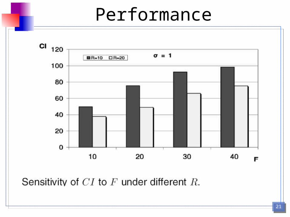
Performance• Qi ： The number of regions with at least one sensor at initial

deployment.

• Qo ： The number of regions with at least one sensor after the movement plan determined by our solution is executed.

• CI = Qo – Qi (Coverage Improvement)

• FD=J/Qo – Qi (Denoting J as the optimal number of flips as determined by our solution).

• Network sizes ： 300*300 units and 150*150 units.

• The region sizes are R = 10 and R = 20 units.

• The basic unit of flip distance d = 10 units. C=1 and C=n.

• The number of sensors deployed is equal to the number of regions.

• PN = P/Q (Denoting P as the total number of packets (or messages) sent and Q as the number of regions).

• ： Different distributions in initial deployment.

1919

Performance

2020

Performance

2121

Performance

2222

Performance

2323

Performance

2424

Performance

2525

Outline Introduction Related work

Edmonds-Karp algorithm Assumption

SOLUTION Overview Mobility Model Constructing the Virtual Graph

Performance Conclusion

2626

Conclusion We proposed a minimum-cost maximum-

flow based solution to optimize coverage and the number of flips.

2727

Thanks for your attention