mobile ad hoc networks: modelling, simulation and
TRANSCRIPT

HAL Id: tel-01589632https://hal.archives-ouvertes.fr/tel-01589632
Submitted on 19 Sep 2017
HAL is a multi-disciplinary open accessarchive for the deposit and dissemination of sci-entific research documents, whether they are pub-lished or not. The documents may come fromteaching and research institutions in France orabroad, or from public or private research centers.
L’archive ouverte pluridisciplinaire HAL, estdestinée au dépôt et à la diffusion de documentsscientifiques de niveau recherche, publiés ou non,émanant des établissements d’enseignement et derecherche français ou étrangers, des laboratoirespublics ou privés.
Mobile Ad Hoc Networks: Modelling, Simulation andBroadcast-based Applications
Luc Hogie
To cite this version:Luc Hogie. Mobile Ad Hoc Networks: Modelling, Simulation and Broadcast-based Applications.Modeling and Simulation. Université du Luxembourg, Faculté des Sciences, de la Technologie et dela Communication [FSTC]; Université du Havre, 2007. English. tel-01589632

University of Le Havre (France)
University of Luxembourg (Luxembourg)
Luc HogieEuropean Ph.D thesis in Computer Science
Mobile Ad Hoc Networks:Modelling, Simulation and Broadcast-based
Applications
Composition of the jury:
Alain Cardon President of the jury University of Paris VI (FR)
Pascal Bouvry Supervisor University of Luxembourg (LU)
Frederic Guinand Supervisor University of Le Havre (FR)
Serge Chaumette Reviewer University of Bordeaux (FR)
Marco conti Reviewer CNR, Pisa (IT)
Steffen Rothkugel Member University of Luxembourg (LU)
Enrique Alba Member University of Malaga (ES)
Michel Syska Member INRIA/University of Nice (FR)
Defended the 18th April 2007.

2

Contents
Contents 3
I Ad hoc networking: generalities 25
1 Definition for “ad hoc network” 28
1.1 Definitions from the literature . . . . . . . . . . . . . . . . . . . . . . . . . . 28
1.1.1 IEEE802.11 specification . . . . . . . . . . . . . . . . . . . . . . . . 29
1.1.2 Stojmenovic and Wu . . . . . . . . . . . . . . . . . . . . . . . . . . . 29
1.1.3 Bhaskar . . . . . . . . . . . . . . . . . . . . . . . . . . . . . . . . . . 30
1.1.4 Gerla . . . . . . . . . . . . . . . . . . . . . . . . . . . . . . . . . . . 30
1.1.5 MobileMANs . . . . . . . . . . . . . . . . . . . . . . . . . . . . . . . 31
1.1.6 Delay Tolerant Networks . . . . . . . . . . . . . . . . . . . . . . . . 31
1.2 Synthetic definition . . . . . . . . . . . . . . . . . . . . . . . . . . . . . . . . 32
2 Ad hoc networking technologies 34
2.1 Packet radio . . . . . . . . . . . . . . . . . . . . . . . . . . . . . . . . . . . . 34
2.1.1 AMPRNet . . . . . . . . . . . . . . . . . . . . . . . . . . . . . . . . 35
2.2 IEEE802.11 . . . . . . . . . . . . . . . . . . . . . . . . . . . . . . . . . . . . 35
2.2.1 IEEE802.11a . . . . . . . . . . . . . . . . . . . . . . . . . . . . . . . 35
2.2.2 IEEE802.11b . . . . . . . . . . . . . . . . . . . . . . . . . . . . . . . 36
2.2.3 IEEE802.11g . . . . . . . . . . . . . . . . . . . . . . . . . . . . . . . 36
2.2.4 IEEE802.11n . . . . . . . . . . . . . . . . . . . . . . . . . . . . . . . 37
2.3 Bluetooth . . . . . . . . . . . . . . . . . . . . . . . . . . . . . . . . . . . . . 37
2.4 Hiperlan . . . . . . . . . . . . . . . . . . . . . . . . . . . . . . . . . . . . . . 37
2.5 BLAST . . . . . . . . . . . . . . . . . . . . . . . . . . . . . . . . . . . . . . 38
2.6 ZigBee . . . . . . . . . . . . . . . . . . . . . . . . . . . . . . . . . . . . . . . 38
2.7 Broadband wireless networking . . . . . . . . . . . . . . . . . . . . . . . . . 38
2.8 Adequation to ad hoc networking and issues . . . . . . . . . . . . . . . . . . 39
2.8.1 Synchronization issue . . . . . . . . . . . . . . . . . . . . . . . . . . 39
3

2.8.2 Latency of the discovery . . . . . . . . . . . . . . . . . . . . . . . . 40
3 Target applications 42
3.1 Vehicular ad hoc networks . . . . . . . . . . . . . . . . . . . . . . . . . . . . 42
3.2 Sensing . . . . . . . . . . . . . . . . . . . . . . . . . . . . . . . . . . . . . . 43
3.3 Personal area networking . . . . . . . . . . . . . . . . . . . . . . . . . . . . 43
3.4 Military systems . . . . . . . . . . . . . . . . . . . . . . . . . . . . . . . . . 44
3.5 Peer-to-peer computing . . . . . . . . . . . . . . . . . . . . . . . . . . . . . 44
3.6 Risk management . . . . . . . . . . . . . . . . . . . . . . . . . . . . . . . . . 45
3.7 Advertising . . . . . . . . . . . . . . . . . . . . . . . . . . . . . . . . . . . . 45
II Simulation 47
4 State of the Art 51
4.1 Testbeds . . . . . . . . . . . . . . . . . . . . . . . . . . . . . . . . . . . . . . 51
4.1.1 Some testbeds . . . . . . . . . . . . . . . . . . . . . . . . . . . . . . 52
4.1.2 Issues . . . . . . . . . . . . . . . . . . . . . . . . . . . . . . . . . . . 52
4.1.3 Proposed solutions . . . . . . . . . . . . . . . . . . . . . . . . . . . . 53
4.2 Existing simulators . . . . . . . . . . . . . . . . . . . . . . . . . . . . . . . . 53
4.2.1 Major simulators . . . . . . . . . . . . . . . . . . . . . . . . . . . . . 54
4.2.1.1 ns-2 . . . . . . . . . . . . . . . . . . . . . . . . . . . . . . . 54
4.2.1.2 GloMoSim . . . . . . . . . . . . . . . . . . . . . . . . . . . 56
4.2.1.3 OPNet . . . . . . . . . . . . . . . . . . . . . . . . . . . . . 56
4.2.1.4 OMNET++ . . . . . . . . . . . . . . . . . . . . . . . . . . 57
4.2.1.5 QualNet . . . . . . . . . . . . . . . . . . . . . . . . . . . . 57
4.2.1.6 GTNets . . . . . . . . . . . . . . . . . . . . . . . . . . . . . 57
4.2.2 Some custom simulators . . . . . . . . . . . . . . . . . . . . . . . . . 58
4.2.2.1 NAB . . . . . . . . . . . . . . . . . . . . . . . . . . . . . . 58
4.2.2.2 SWANS . . . . . . . . . . . . . . . . . . . . . . . . . . . . . 58
4.2.2.3 J-Sim . . . . . . . . . . . . . . . . . . . . . . . . . . . . . . 58
4.2.2.4 Jane . . . . . . . . . . . . . . . . . . . . . . . . . . . . . . . 59
4.2.2.5 Dianemu . . . . . . . . . . . . . . . . . . . . . . . . . . . . 59
4.2.3 Simulation languages and frameworks . . . . . . . . . . . . . . . . . 59
4.2.4 Which simulator for what need? . . . . . . . . . . . . . . . . . . . . 60
4.3 Issues . . . . . . . . . . . . . . . . . . . . . . . . . . . . . . . . . . . . . . . 60
4.3.1 The accuracy of mobile ad hoc networks simulators . . . . . . . . . . 61
4.3.1.1 The impact of granularity . . . . . . . . . . . . . . . . . . . 61
4.3.1.2 Mobility models . . . . . . . . . . . . . . . . . . . . . . . . 61
4

4.3.1.3 Radio propagation models . . . . . . . . . . . . . . . . . . 62
4.3.1.4 Number of simulated nodes . . . . . . . . . . . . . . . . . . 63
4.3.2 Simulation acceleration techniques . . . . . . . . . . . . . . . . . . . 63
4.3.2.1 Parallelism and distribution . . . . . . . . . . . . . . . . . 63
4.3.2.2 Staged simulation . . . . . . . . . . . . . . . . . . . . . . . 64
4.3.2.3 Bining . . . . . . . . . . . . . . . . . . . . . . . . . . . . . . 65
4.3.2.4 Statistical simulations . . . . . . . . . . . . . . . . . . . . . 65
4.3.3 Visualization and debugging facilities . . . . . . . . . . . . . . . . . 66
4.4 New trends in mobile ad hoc networks simulation . . . . . . . . . . . . . . . 66
4.4.1 Application-level simulation . . . . . . . . . . . . . . . . . . . . . . . 68
5 The Madhoc simulator 69
5.1 Objectives . . . . . . . . . . . . . . . . . . . . . . . . . . . . . . . . . . . . . 69
5.2 Network model . . . . . . . . . . . . . . . . . . . . . . . . . . . . . . . . . . 70
5.2.1 Models for the hardware . . . . . . . . . . . . . . . . . . . . . . . . . 70
5.2.1.1 Different devices . . . . . . . . . . . . . . . . . . . . . . . . 70
5.2.1.2 Different networking technologies . . . . . . . . . . . . . . . 71
5.2.1.3 Different computational/storage capacities . . . . . . . . . 72
5.2.2 Models for the communication links . . . . . . . . . . . . . . . . . . 72
5.2.2.1 PHY and MAC layer . . . . . . . . . . . . . . . . . . . . . 72
5.2.2.2 Network layer . . . . . . . . . . . . . . . . . . . . . . . . . 75
5.2.2.3 Application layer . . . . . . . . . . . . . . . . . . . . . . . . 76
5.2.2.4 Heterogeneous networks . . . . . . . . . . . . . . . . . . . . 76
5.3 Models for ad hoc applications . . . . . . . . . . . . . . . . . . . . . . . . . 78
5.3.1 Connections/disconnections . . . . . . . . . . . . . . . . . . . . . . . 79
5.3.2 Application identification . . . . . . . . . . . . . . . . . . . . . . . . 79
5.4 Simulation model . . . . . . . . . . . . . . . . . . . . . . . . . . . . . . . . . 79
5.4.1 Time management . . . . . . . . . . . . . . . . . . . . . . . . . . . . 79
5.4.1.1 Discrete-time simulation . . . . . . . . . . . . . . . . . . . 80
5.4.1.2 Simulator internal scheduler . . . . . . . . . . . . . . . . . 80
5.4.2 Simulation area and network projections . . . . . . . . . . . . . . . . 81
5.4.3 Monitoring the ad hoc applications . . . . . . . . . . . . . . . . . . . 82
5.4.4 Termination of the simulation process . . . . . . . . . . . . . . . . . 82
5.4.5 Random number generation . . . . . . . . . . . . . . . . . . . . . . . 83
6 Modelling Mobility 84
6.1 State of the Art . . . . . . . . . . . . . . . . . . . . . . . . . . . . . . . . . . 84
6.1.1 Preliminary discussion . . . . . . . . . . . . . . . . . . . . . . . . . . 84
6.1.2 Mobility models in use . . . . . . . . . . . . . . . . . . . . . . . . . . 85
5

6.1.2.1 Random walk mobility . . . . . . . . . . . . . . . . . . . . 85
6.1.2.2 Random waypoint mobility . . . . . . . . . . . . . . . . . . 86
6.1.2.3 Obstacle mobility model . . . . . . . . . . . . . . . . . . . 86
6.1.2.4 City-section mobility . . . . . . . . . . . . . . . . . . . . . 86
6.1.2.4.1 City Section Mobility Model . . . . . . . . . . . . 87
6.1.2.4.2 Manhattan mobility model . . . . . . . . . . . . . 87
6.1.2.5 Group mobility models . . . . . . . . . . . . . . . . . . . . 87
6.1.2.5.1 Reference point group mobility . . . . . . . . . . . 87
6.1.2.5.2 Columobile node mobility model . . . . . . . . . . 88
6.1.2.5.3 Nomadic community mobility model . . . . . . . . 88
6.1.2.5.4 Pursue Mobility Model . . . . . . . . . . . . . . . 88
6.1.2.6 Boundless Simulation Area . . . . . . . . . . . . . . . . . . 88
6.1.3 Characterizing mobility models . . . . . . . . . . . . . . . . . . . . . 89
6.1.3.1 Space/speed distribution . . . . . . . . . . . . . . . . . . . 89
6.1.3.2 Link duration . . . . . . . . . . . . . . . . . . . . . . . . . 89
6.1.3.3 Degree distribution . . . . . . . . . . . . . . . . . . . . . . 90
6.1.3.4 Neighbor density . . . . . . . . . . . . . . . . . . . . . . . . 90
6.2 A new classification for mobility models . . . . . . . . . . . . . . . . . . . . 90
6.2.1 Randomness . . . . . . . . . . . . . . . . . . . . . . . . . . . . . . . 90
6.2.2 Traces . . . . . . . . . . . . . . . . . . . . . . . . . . . . . . . . . . . 91
6.2.3 Group/entity . . . . . . . . . . . . . . . . . . . . . . . . . . . . . . . 91
6.2.4 Memoryful/less . . . . . . . . . . . . . . . . . . . . . . . . . . . . . . 91
6.2.5 Spatial constraints . . . . . . . . . . . . . . . . . . . . . . . . . . . . 92
6.2.6 Plurality . . . . . . . . . . . . . . . . . . . . . . . . . . . . . . . . . . 92
6.2.7 Application-driven . . . . . . . . . . . . . . . . . . . . . . . . . . . . 92
6.3 New metrics for mobility models . . . . . . . . . . . . . . . . . . . . . . . . 92
6.3.1 Size of the greatest connected component . . . . . . . . . . . . . . . 92
6.3.2 Probability of meeting again . . . . . . . . . . . . . . . . . . . . . . 93
6.4 Human mobility . . . . . . . . . . . . . . . . . . . . . . . . . . . . . . . . . 93
6.4.1 Algorithm . . . . . . . . . . . . . . . . . . . . . . . . . . . . . . . . . 93
6.4.2 Radio waves . . . . . . . . . . . . . . . . . . . . . . . . . . . . . . . . 94
6.4.3 Scenarios . . . . . . . . . . . . . . . . . . . . . . . . . . . . . . . . . 94
6.4.3.1 Mall . . . . . . . . . . . . . . . . . . . . . . . . . . . . . . . 94
6.4.3.2 City-center . . . . . . . . . . . . . . . . . . . . . . . . . . . 94
6.4.3.3 Highway . . . . . . . . . . . . . . . . . . . . . . . . . . . . 95
6.4.4 Open issues . . . . . . . . . . . . . . . . . . . . . . . . . . . . . . . . 96
6.4.4.1 Initialization of the mobility . . . . . . . . . . . . . . . . . 96
6.4.4.2 Defining the resolution of the simulation . . . . . . . . . . 97
6

III Broadcasting across mobile ad hoc networks 99
7 State of the Art 101
7.1 Technical challenges . . . . . . . . . . . . . . . . . . . . . . . . . . . . . . . 102
7.1.1 Hidden and exposed node problems . . . . . . . . . . . . . . . . . . 102
7.1.2 Mobility and Partitioning . . . . . . . . . . . . . . . . . . . . . . . . 102
7.2 Protocols . . . . . . . . . . . . . . . . . . . . . . . . . . . . . . . . . . . . . 102
7.2.1 Simple Flooding . . . . . . . . . . . . . . . . . . . . . . . . . . . . . 103
7.2.2 Probabilistic scheme . . . . . . . . . . . . . . . . . . . . . . . . . . . 103
7.2.3 Distance-based methods . . . . . . . . . . . . . . . . . . . . . . . . . 103
7.2.4 Area-based methods . . . . . . . . . . . . . . . . . . . . . . . . . . . 103
7.2.5 Flooding with Self-Pruning . . . . . . . . . . . . . . . . . . . . . . . 104
7.2.6 Scalable Broadcast Algorithm . . . . . . . . . . . . . . . . . . . . . . 104
7.2.7 Multipoint relaying . . . . . . . . . . . . . . . . . . . . . . . . . . . . 104
7.2.8 Ad Hoc Broadcast Protocol (AHBP) . . . . . . . . . . . . . . . . . . 104
7.2.9 AHBP-EX . . . . . . . . . . . . . . . . . . . . . . . . . . . . . . . . . 105
7.2.10 INOP . . . . . . . . . . . . . . . . . . . . . . . . . . . . . . . . . . . 105
7.3 Classifications . . . . . . . . . . . . . . . . . . . . . . . . . . . . . . . . . . . 105
7.3.1 Camp’s classification . . . . . . . . . . . . . . . . . . . . . . . . . . . 105
7.3.2 Stojmenovic’s classification . . . . . . . . . . . . . . . . . . . . . . . 106
7.3.3 Wu’s classification . . . . . . . . . . . . . . . . . . . . . . . . . . . . 107
8 DFCN 108
8.1 Objectives . . . . . . . . . . . . . . . . . . . . . . . . . . . . . . . . . . . . . 108
8.2 Requirements . . . . . . . . . . . . . . . . . . . . . . . . . . . . . . . . . . . 110
8.3 DFCN’s strategy . . . . . . . . . . . . . . . . . . . . . . . . . . . . . . . . . 111
8.3.1 Description of the algorithm . . . . . . . . . . . . . . . . . . . . . . . 111
8.3.1.1 Message reception event . . . . . . . . . . . . . . . . . . . . 112
8.3.1.2 RAD expiration event . . . . . . . . . . . . . . . . . . . . . 113
8.3.1.3 New neighbor event . . . . . . . . . . . . . . . . . . . . . . 113
8.3.2 Reactivity and Proactivity in DFCN . . . . . . . . . . . . . . . . . . 114
8.3.2.1 Reactive behavior . . . . . . . . . . . . . . . . . . . . . . . 114
8.3.2.2 Proactive behavior . . . . . . . . . . . . . . . . . . . . . . . 115
8.3.2.3 Reactive and proactive coupled . . . . . . . . . . . . . . . . 116
8.3.2.4 Application domain . . . . . . . . . . . . . . . . . . . . . . 117
8.4 Experiments . . . . . . . . . . . . . . . . . . . . . . . . . . . . . . . . . . . . 117
8.4.1 Description of the experiments . . . . . . . . . . . . . . . . . . . . . 118
8.4.1.1 Node mobility . . . . . . . . . . . . . . . . . . . . . . . . . 118
8.4.1.2 PHY/MAC . . . . . . . . . . . . . . . . . . . . . . . . . . . 119
7

8.4.1.3 Radio wave propagation . . . . . . . . . . . . . . . . . . . . 119
8.4.1.4 Parameters of the protocol . . . . . . . . . . . . . . . . . . 120
8.4.1.5 Benchmarking process . . . . . . . . . . . . . . . . . . . . . 120
8.4.2 Results . . . . . . . . . . . . . . . . . . . . . . . . . . . . . . . . . . 121
8.4.2.1 Number of emissions . . . . . . . . . . . . . . . . . . . . . . 122
8.4.2.2 Number of redundant receptions . . . . . . . . . . . . . . . 122
8.4.2.3 Duration of the broadcasting process . . . . . . . . . . . . 122
8.4.2.4 Emission efficiency . . . . . . . . . . . . . . . . . . . . . . . 123
8.4.2.5 Application to different topologies . . . . . . . . . . . . . . 123
9 Optimization of the broadcasting process 126
9.1 Genetic optimization . . . . . . . . . . . . . . . . . . . . . . . . . . . . . . . 126
9.2 Multi-objective optimization . . . . . . . . . . . . . . . . . . . . . . . . . . . 126
9.3 The DFCNT problem . . . . . . . . . . . . . . . . . . . . . . . . . . . . . . 127
9.3.1 Using a cellular genetic algorithm . . . . . . . . . . . . . . . . . . . . 128
9.3.1.1 Targeted network . . . . . . . . . . . . . . . . . . . . . . . 128
9.3.1.2 Experiments . . . . . . . . . . . . . . . . . . . . . . . . . . 130
9.3.2 Using scatter search . . . . . . . . . . . . . . . . . . . . . . . . . . . 132
9.3.2.1 Multi-objective Scatter Search . . . . . . . . . . . . . . . . 132
9.3.2.1.1 Scatter Search . . . . . . . . . . . . . . . . . . . . 132
9.3.2.1.2 AbSS . . . . . . . . . . . . . . . . . . . . . . . . . 133
9.3.2.2 Targeted network . . . . . . . . . . . . . . . . . . . . . . . 133
9.3.2.3 Results . . . . . . . . . . . . . . . . . . . . . . . . . . . . . 134
9.3.2.3.1 Metrics . . . . . . . . . . . . . . . . . . . . . . . . 134
9.3.2.3.2 Parametrization . . . . . . . . . . . . . . . . . . . 134
9.3.2.3.3 Results . . . . . . . . . . . . . . . . . . . . . . . . 135
9.4 The cDFCNT problem . . . . . . . . . . . . . . . . . . . . . . . . . . . . . . 136
9.4.1 Results . . . . . . . . . . . . . . . . . . . . . . . . . . . . . . . . . . 138
Bibliography 143
Index 158
List of Figures 162
List of Tables 164
8

Summary
Over the last few years, personal communication devices have invaded most developed
countries and today, the majority of the population owns a mobile phone and most people
use personal digital assistants, mobile computers, etc. This tendency is reinforced and
occurs at the same time with a new trend: most of these devices get equipped with one or
several wireless networking interfaces. Practically, Wi-Fi or/and Bluetooth-enabled devices
become of frequent use. More than allowing the connection to some access point (which
can be found in airports, train stations, city-centers, restaurants, etc), these interfaces
also permit to interconnect directly with one another in a decentralized way and hence to
self-organize into “ad hoc networks”.
A mobile ad hoc network is a set of mobile nodes able to communicate with other nodes
in their surroundings. These wireless communications happen in a peer-to-peer manner,
without relying on any predefined infrastructure. Today, mobile ad hoc networks are
mainly used for sensing, gaming and military purposes. But the steadily wider adoption
of wireless technologies in daily life let one foresee the next generation of mobile ad hoc
network applications: environmental and medical monitoring, groupware, customer-to-
customer applications, risk management, entertainment, advertising, etc. In this document
we will consider a subclass of mobile ad hoc network called “delay tolerant networks”. In
such network, the mobility is hardly predictable and the disruption of connection is a
common and normal phenomenon.
In order to enable the development and spreading of these applications, a number
of issues have to be solved. First, in such networks, end-to-end connectivity cannot be
guaranteed. Indeed mobile ad hoc networks may be partitioned and nodes may be spo-
radically present in the network. As such, mobile ad hoc networks can be considered as
Delay Tolerant Networks (DTN). Second, the topology of the network changes over time
because of the mobility of the stations. Then, the way the communication primitives were
implemented in the context of wired networks is no longer applicable. It is hence necessary
to propose new algorithms to take those primitives into account, like broadcasting that
serves as a basic pattern for the design of many mobile ad hoc network applications.
The design and implementation of such communication schemes, and more generally
of mobile ad hoc network applications, can be achieved using two different ways: either
9

by building a real network, or by resorting to modelling and simulation. Theoretical
approaches failed at modeling the inherent complexity of mobile ad hoc networks in a
comprehensive manner. Indeed, ad hoc networks are decentralised systems which are
ruled by a variety of elements including radio signal, network traffic, mobility, collaborative
behavior, etc. If theoretical approaches certainly are useful for represent one or the other
elements, they do not suit the modelling of a system as a whole. In the context of this
work, where city-scale environment were considered, simulation was hence unavoidable.
The development of such simulators took place at the crossroad of some projects in
relation to complex system modelling, optimization and middleware design for mobile ad
hoc networks, and conducted in several European countries.
This diversity led to the design of a custom simulator called Madhoc. Indeed the
mobile ad hoc simulators which are already available on the market most often are designed
in such a way they allow the simulation of specific applications. They also generally suffer
from a complex architecture (often poorly documented) that make them hardly adaptable
to other applications. Consequently, none of them apparently turn out to be flexible enough
so as it would have met our diverse needs. Madhoc captures the major characteristics of
DTNs, by providing an extendable set of mobility models as well as a framework for the
definition of new applications.
By looking at the State of Art protocols for mobile ad hoc networks and delay tolerant
networks, it appeared that the broadcast issue had not yet been solved in a satisfactory
manner. Indeed none of the protocols proposed so far proceed nicely in specific conditions
of delay tolerant networking. Madhoc was then primarily used for the investigation of the
broadcasting issue. In this specific context, networks composed of thousands devices using
a variety of wireless technologies were considered. These networks are partitioned and ex-
hibit heterogeneous densities. This led to the design of a bandwidth-efficient broadcasting
protocol called DFCN.
10

Resume
Au cours des dernieres annees, l’utilisation de telephones mobiles, d’ordinateurs portables
et, dans une moindre mesure, d’assistants personnels a explose. Le phenomene est tel que
dans les pays industrialises, la quasi-totalite de la population utilise un telephone mobile.
Dans le meme temps, la majorite de ces equipements se voit associee a une interface pour
reseau mobile, en particulier Wi-Fi et/ou Bluetooth. En plus de permettre la connection a
Internet par le biais de points d’acces, ces technologies permettent aux machines mobiles
de se connecter de facon decentralisee et par la meme de s’auto-organiser en “reseaux
mobiles ad hoc”.
Un reseau mobile ad hoc est un ensemble de nœuds mobiles capables de communiquer
avec les nœuds presents a proximite geographique. Ces communications sans-fil operent
en mode pair-a-pair : elles se passent d’infrastructure de telecommunication. A l’heure a
laquelle ces lignes sont ecrites, les reseaux mobiles ad hoc sont principalement utilises dans
le cadre de reseaux de capteurs, pour les applications de jeux et les applications militaires.
Cependant, l’adoption croissante des technologies de reseau sans-fil par le grand public
permet d’entrevoir les applications futures : surveillance environnementale et medicale,
travail en equipe, applications entre particuliers, gestion du risque industriel, publicite,
etc.
Pourtant, afin que ces applications soient realisables, un certain nombre de problemes
doivent toujours etre solutionnes. En premier lieu, dans les reseaux mobile ad hoc, il n’est
pas possible de garantir qu’il existe un chemin entre deux nœuds donnes. En effet le reseau
peut etre partitionne et la presence des nœuds est sporadique. En second lieu, a cause de
la mobilite des nœuds, la topologie du reseau change au cours du temps. De ce fait, les
implementations courantes des primitives reseau ne sont plus utilisables. Il est necessaire
de proposer de nouveaux algorithmes permettant l’utilisation de ces primitives dans le
cadre contraint des reseaux mobiles ad hoc. Ces primitives incluent la diffusion, qui est
une pierre de base de nombreuses applications pour reseaux ad hoc.
L’experimentation de services (ou plus generalement d’applications) pour reseaux mo-
biles ad hoc peut etre effectuee soit sur des reseaux dedies (appeles testbeds), soit sur des
simulateurs logiciels. Dans le cadre des travaux presentes dans cette these, pour lesquels
un environement de type urbain est considere, la simulation s’est averee inevitable.
11

Le developpement d’un tel simulateur s’est opere dans le cadre de plusieurs projets
lies aux systemes complexes, a l’optimisation et a la conception d’intergiciel. Ces projets
impliquent des universites de differents pays d’Europe.
Cette diversite des besoins a conduit a la conception d’un simulateur dedie, appele
Madhoc. Madhoc considere un certain nombre de caracteristiques des reseaux mobiles
ad hoc en proposant un ensemble de modeles de mobilite ainsi qu’une interface de pro-
grammation pour la definition de nouvelles applications.
Madhoc a ete initialement utilise pour l’experimentation de protocoles de diffusion
dans le cadre de reseaux heterogenes de grande taille (reseaux impliquant plusieurs milliers
de nœuds, et plusieurs technologies reseaux). Ces reseaux sont generalement partitionnes
et ont des densites non-homogenes. Ceci nous a amene au developpement de DFCN: un
protocole de diffusion efficace en terme de bande passante utilisee.
12

Kuerzfaassung
Dei lescht Joeren ass de Gebrauch vun de Mobiltelefonnen, de Laptoppen an an engem
manner groussen Emfang, de perseinlechen Hellefsapparater, explodeiert. De Phanomen
ass esou grouss, datt an den Industrielanner praktesch jiddereen en Handy benotzt. Eng
Majoriteit vun desen Equipementer gi mat enger Interface vu mobilen Netzer verbonnen,
besonnesch dem Wi-Fi ana/oder Bluetooth. Des Technologien ermeiglechen de mobile
Maschinnen net nemmen eng Verbindung mat Internet duerch Zougankspunkten, ma och
sech dezentraliseiert unzeschleissen an doduerch selbststannesch a Smobil Netzer ad hocT
ze organiseieren.
En zweckmeissegt Mobilnetz ass en Ensembel vu mobile Kniet, dei faeg si mat anere
mobile Punkten, dei sech an engem noe geografesche Beraich befannen, ze kommunizeieren.
Des kabellos Kommunikatioune verfuere no der binomer Method : si brauche keng telekom-
munikativ Infrastruktur. Momentan ginn des Netzer haaptsachlech am Beraich vun Em-
fangsnetzer fir d’Appikatioune vu Spiller an och fir dei vum Militar benotzt. Dese wuessende
Gebrauch vun de kabellosen Netztechnologien duerch d’Effentlechkeet erlaabt ons dei
zoukenfteg Applikatioune virauszegesinn : Iwwerwaachung vun der Emwelt an am medezi-
nesche Beraich, Applikatiounen teschent privat Leit, Verwaltung vum Industrierisiko, Pub-
liciteit asw. Fir des Applikatiounen ausschaffen ze kennen, mussen awer nach gewesse
Problemer geleist ginn. Eischtens kann an de mobilen Netzer ad hoc net garanteiert ginn,
datt et e Wee teschent zwee bestemmte Kniet gett. An der Tat kann d’Netz gedeelt an
d’Virkomme vun de Punkte sporadesch sinn. Zweetens annert sech duerch d’Mobiliteit vun
de Kniet d’Topologie vum Netz mat der Zait. Doduerch gett et onmeiglech dei gangesch
praktesch Emsetzunge vun de Primitiven vum Netz ze benotzen. Et ass also neideg nei
Algorithme virzeschloen, dei de Gebrauch vun dese Primitiven am ageschrankte Kader
vun de mobilen Netzer ad hoc ermeiglechen. Des Primitive begraifen d’Verbreedung, dei
eng vun de Grondforme vu villen Appikatioune fir d’ad hoc Netzer duerstellt.
D’Experimentatioune vu Servicer (oder mei allgemeng vun Applikatiounen) fir mobil
Netzer ad hoc kenne souwoul op adequaten Netzer (sougenannten testbeds), wei och mat
Simulatiounslogiciellen erfollegen. Am Kader vun de virgestallten Aarbechten an deser
Thes fir dei en urbanen Typ a Betracht gezu ginn ass, huet missen op d’Simulatioun
zereckgegraff ginn.
13

D’Entwecklung vu sou engem Simulator ass am Kader vun etleche Projekter, dei mat
komplexe Systemer verbonne sinn, an d’Optimisatioun an d’Konzeptioun vun Intergiciel
ermeiglecht hunn. Un dese Projekter sinn Universiteite vu verschiddenen europaesche
Lanner bedeelegt.
D’Diversiteit vun de Bedierfnesser huet zu der Konzeptioun vun engem adequate Sim-
ulator gefouert, dem Madhoc. Madhoc betruecht eng gewessen Unzuel vun Eegeschafte
vun de mobilen Netzer ad hoc an deems en en Ensembel vu Mobilmodeller, wei och eng
Programmatiounsinterface fir d’Definitioun vun neien Applikatioune virschleit.
Madhoc ass am Ufank fir d’Experimentatiounen vun de Verdeelerprotokollen am
Kader vu groussen heterogenen Netzer (Netzer, dei e puer dausend Kniet emfaassen a
verschidden technologesch Netzer) benotzt ginn. Des Netzer sinn am allgemenge gedeelt
an hu keng homogen Dichten. Dat huet zu der Entwecklung vum DFCN gefouert: e
wierksamen Diffusionsprotokoll duerch dei gebrauchten Reseauskapaziteit.
Special thanks to Jeanne Meskens, who translated the abstract into Luxembourgish.
14

Acknowledgments
I first want to give great thanks to Pascal Bouvry, Frederic Guinand who taught me the
way a scientific research project should be conducted and permitted me to turn four years
of research into the highest academic diploma. I am also willing to express my gratitude
to Serge Chaumette, Marco Conti, Enrique Alba, Gianni Di Caro, Michel Syska, Alain
Cardon and Steffen Rothkugel and all the scientists who dedicated some of their precious
time at evaluating my work and at advising me.
I would like to congratulate Gregoire Danoy, Marcin Seredynski, all my other col-
leagues, and again Pascal and Frederic for being so pleasant to work with, and for being
so friendly persons.
I am willing to thank the Luxembourg Ministry of Research (and Ms. Entringer) as
well as Luxembourg University which permitted me to get into Research by providing me,
respectively, a PhD grant (Bourse Formation Recherche) and subsequently a contract as
a teaching assistant in the Computer Science department.
I want to thank Nadege for having been so patient with the boring computer-junkie
I certainly was during those PhD years. A special thank goes to Elisa for having made
me much more happy—and busy—that I would have been otherwise during the past year.
The last thankya goes to my adorable parents who never failed at advising me the right
way to go.
Finally, I want to thank all of those that I forget to thank inhere. They hopefully will
forgive me for forgetting.
15

16

Introduction
Recent studies performed by popular technology magazines like Point Topic 1and DSL
Forum2 stated the number of citizens equipped with a broadband access to the Internet has
followed an amazing increase: a growth of 40% per year since 2000. Moreover, most current
commercial offers include a DSL-Wifi router, making people more and more comfortable
with this technology. At the same time, small communicating objects – PDA, mobile
phones, multimedia players, gaming console, etc – are becoming more and more common
in our daily life. For instance, the spreading ratio of mobile phones is close to 100% in most
western European and Northern American regions. In addition, it is noticeable that next
generations of most of them come with Wi-Fi interfaces: more and more mobile phones are
now able to communicate using the traditional GSM/UMTS media but also using wireless
interfaces, and cumulate the features of classical mobile phones, PDAs, multimedia players
and even gaming consoles. This general tendency leads us to envision a future in which
most people will be equipped with devices able to communicate using wireless interfaces.
Oppositely to classical wired network, in a Wi-Fi network the nodes communicate by
sending and receiving electro-magnetic (radio) waves. Wi-Fi networks can operate in two
modes: “infrastructure” and “ad hoc”. In infrastructure mode, the nodes communicate
with each other via an access point. This access point rules the communications in the
local wireless network (WirelessLAN). Most often, the access point also enables the nodes
within the WirelessLAN to communicate with nodes outside of the network (access to the
internet in particular). This mode, which is the default one for most Wi-Fi devices, is com-
monly used in public places were access to the internet is provided (train stations, airports,
etc), at home, and in the company. In ad hoc mode, nodes communicate directly without
resorting to any infrastructure. Although this mode is not commonly used, it presents
some advantages. In particular ad hoc communications require neither the construction of
expensive infrastructure nor network administration. Unfortunately ad hoc networks face
a number of difficulties which have to be solved in order to permit their deployment. In
ad hoc mode, a set of devices can build in an autonomous and spontaneous way a commu-
nication network and have the capacity to self-organize in order to maintain it. This kind
1http://point-topic.com/2http://www.dslforum.org/
17

of network is gaining interest, although it is so far limited to gaming or to the building of
temporary networks for answering peculiar situations for which a communication network
is required for assisting a group of people in its action when no infrastructure is available.
All along this document, the focus will be put on mobile ad hoc networks, as they are
defined in the following.
Mobile ad hoc networks are wireless networks built on-the-fly by mobile computers
(also called “nodes”, “terminals” or “stations”) getting in and out of range with each oth-
ers. In the literature, mobile ad hoc networks are also commonly referred to as MANETs.
Two important keywords for mobile ad hoc networking are “radio communication” and
“mobility”. On the one hand, because the nodes have a limited radio range, nodes can
communicate using the radio communication medium if they are close to each other (in
that case one say that the nodes are in range). This is not enough however. Wireless
communication exhibits a variety of issues which lead to some situations where the com-
munication between two nodes in range fails, or two nodes in range do not detect each
other. On the other hand, node mobility heavily impacts the connectivity of the network.
The way the nodes move (note that not necessarily all of them move, though) results in
a variety of topologies and dynamic properties of the network. For example, in a network
in which the nodes move in a random way, no connection can be assumed durable; but in
a network in which the nodes move in groups, then the creation of long-lived clusters may
occur. These characteristics lead to a situation in which the current implementation of the
common network operations (broadcast, unicast, routing, etc) is not applicable. Indeed
enabling these operations in mobile ad hoc networks is achievable only by providing new
implementations that handle parameters like dynamic network discovery, delays, etc.
All along this document, we will consider a subclass of mobile ad hoc networks, called
delay tolerant networks. One of the most prominent properties of delay tolerant networks
are a high and unpredictable mobility and disruption of the network connections.
A variety of technologies already enable mobile ad hoc networking. The most commonly
referred one is the ad hoc mode of the IEEE802.11 class of protocols. On the consumer
market, IEEE802.11 is known as “Wi-Fi”. Bluetooth, whose design apparently suits better
mobile ad hoc networking, is becoming popular in the context of Personal Area Networking
(PAN). Protocols such as Hiperlan, ZigBee, etc, provide alternative—some say better—
solutions to mobile ad hoc networking but, up to now, they sort of failed at attracting
the attention of the research groups. Practically, as of writing, a vast amount of the
papers published on the topic of mobile ad hoc networking present experiments based on
IEEE802.11.
Today, mobile ad hoc networking is a popular area of research which gathers researchers
working on the topics of networking, distributed systems, complex systems, security,
telecommunications, etc. In the future, when mobile ad hoc networks will be deployed
18

at a real scale, they will allow the deployment of applications such as e-commerce, confer-
encing, gaming, mobile grid computing applications, etc.
Today, mobile ad hoc networks are not developed in a real-scale. As a consequence,
mobile ad hoc networks have recourse to experimentation networks (which are named
“testbeds”) or to software simulators ; simulators being apparently the most commonly
used solution. In fact, testbeds exhibit many inherent drawbacks (like their high cost,
the difficulty to built one, the difficulty of monitoring them, etc) which refrain research
laboratories to build and use them. The studies of large-scale applications —which is our
concern— most of the time requires modelling and simulation. Two directions can then
be followed: either using existing (and often general purpose) simulators like ns-2 [ns2],
or conceiving a simulator tailored to specific purposes.
My work occurs in the context of several multi-national academic projects, having sep-
arate requirements. In particular the SoNi project (Luxembourg) [Uni07] —which was the
initial source of funds— targets to providing a middleware solution to application-level ad
hoc communications. This consists in identifying the network properties that play a role
in application-level communication, in proposing an adequate communication paradigm as
well as a set of network primitives, and in an implementing these.
In the context of the GraphStream project (France) [AD07], the MIV team (which is of
subset of the LITIS laboratory (France)) studies dynamic graphs as models for complex
systems. Complex systems are made of many locally interacting entities, which global
behavior is obtained out of local interactions. Particularly, MIV researchers try to put
into light the mechanisms which permit the creation of organizations in such networks.
This work takes place in the context of complex system research. Indeed mobile ad hoc
networks can be considered as complex systems, especially when they exhibit mobility
models which, however based on basic individual behavior, exhibit complex organizational
structures like clusters, chains, etc.
The SARAH project (France) focuses on the design of an experimentation platform allow-
ing the study of Delay Tolerant Networks (DTNs). In this context, a key issue is to couple
a test-bed and a simulator so as the test-bed would be virtually expanded by a simulated
network.
The ABASMUS project [Uni] addresses the issue of topology control for ad hoc networks.
More precisely it aims at providing new topology control protocols by considering “injec-
tion points”—connections from ad hoc nodes to some infrastructure.
Last, researchers at Malaga University needed a simulation tool permitting the genetic
multi-optimization of broadcast protocols. Using some results one single simulation pro-
cess as the value of the fitness function for their optimization algorithms, an issue was to
use a simulator that would be able to operate the simulation of one broadcasting process
in a very short time.
19

Laboratory Resort to simulation for...
Universidad de Malaga (SP) Multi-objective optimization of broadcast protocols
Universite du Luxembourg (LU) Broadcast and topology control protocols
Universite de Bretagne-Sud (FR) Network emulation
Universite du Havre (FR) Generation of dynamic graphs
Universite de Bordeaux (FR) Military applications
Universite de St. Etienne (FR) Topology control protocols
SES/Astra Content delivery in VANETs
Universite de Toulouse (FR) Mobility of agents on ad hoc nets
Table 1: The diversity of applications of Madhoc.
This diversity of requirements of our academic partners imposed the development of
a custom simulator. Table 1 illustrates these needs. In addition to the requirements for-
mulated hereinbefore, from a software engineering point of view, a simulation tool must
provide a comprehensive programming user interface and it must be designed so as incor-
porating new components (mobility models, user applications, metrics, GUI elements, etc)
is easy.
Most studies on mobile ad hoc networking use the random waypoint as a reference
for node mobility [BRS03]. But recent studies have shown that the random waypoint
mobility model fails at reproducing human mobility in an realistic fashion. Moreover,
the simulation settings generally used in experimentation favor the execution of protocols.
When using more realistic mobility as it is presented hereinbefore, many applications, like
broadcasting, no longer operate.
Broadcasting constitutes one of the fundamental low-level network operations which
serves as the basis of higher level applications such as routing. As such, it is one of
the earliest research interests on mobile ad hoc networking. Broadcasting is commonly
considered as an operation which consists in sending a message from one given node (the
source station) to all the nodes in the network. In a decentralized network, the message
that is subject to broadcasting is relayed by intermediate nodes so that all the network
graph is eventually spanned. Unfortunately, this definition cannot be applied in the context
of mobile ad hoc networks. Indeed the limited radio range of the nodes, as well as node
mobility, make that it is very likely that some nodes are unreachable at a given moment.
Consequently, we define as a multi-objective problem targeting at maximizing the number
of nodes reached, at minimizing the time required to reach them, and at minimizing the
network overhead [?]. Minimizing the network overhead is particularly important because
too many emissions is likely to lead a broadcast storm, and the congestion of the network.
Generally when the mobility is an important properties of networks, spanning trees-
20

based methods are applied. These aim at determining the minimal set of relay nodes
that must participate to the broadcast process. Contrarily, when mobility is considered,
different strategy, mostly based neighborhood information, are employed. These include
Probabilistic schemes, Scalable Broadcasting Algorithm (SBA), Multipoint Relaying, Ad
hoc Broadcasting Procotol (AHBP), etc. These strategies work well when the network
is connected, but they fail as soon as partitioning occurs. There exist solutions like the
extension of AHBP (called AHBP-EX) which overcomes this problem by triggering re-
emission on the discovery of a new neighbor. This strategy unfortunately leads to waste
much bandwidth. Additionally, SBA and AHBP, which are the most effective protocols in
their class, require the knowledge of 2-hop neighborhood information (nodes must know
their neighbors, as well as the neighbors of their neighbors). In reality, when the mobility
is high, we assume that 2-hop information is not achievable.
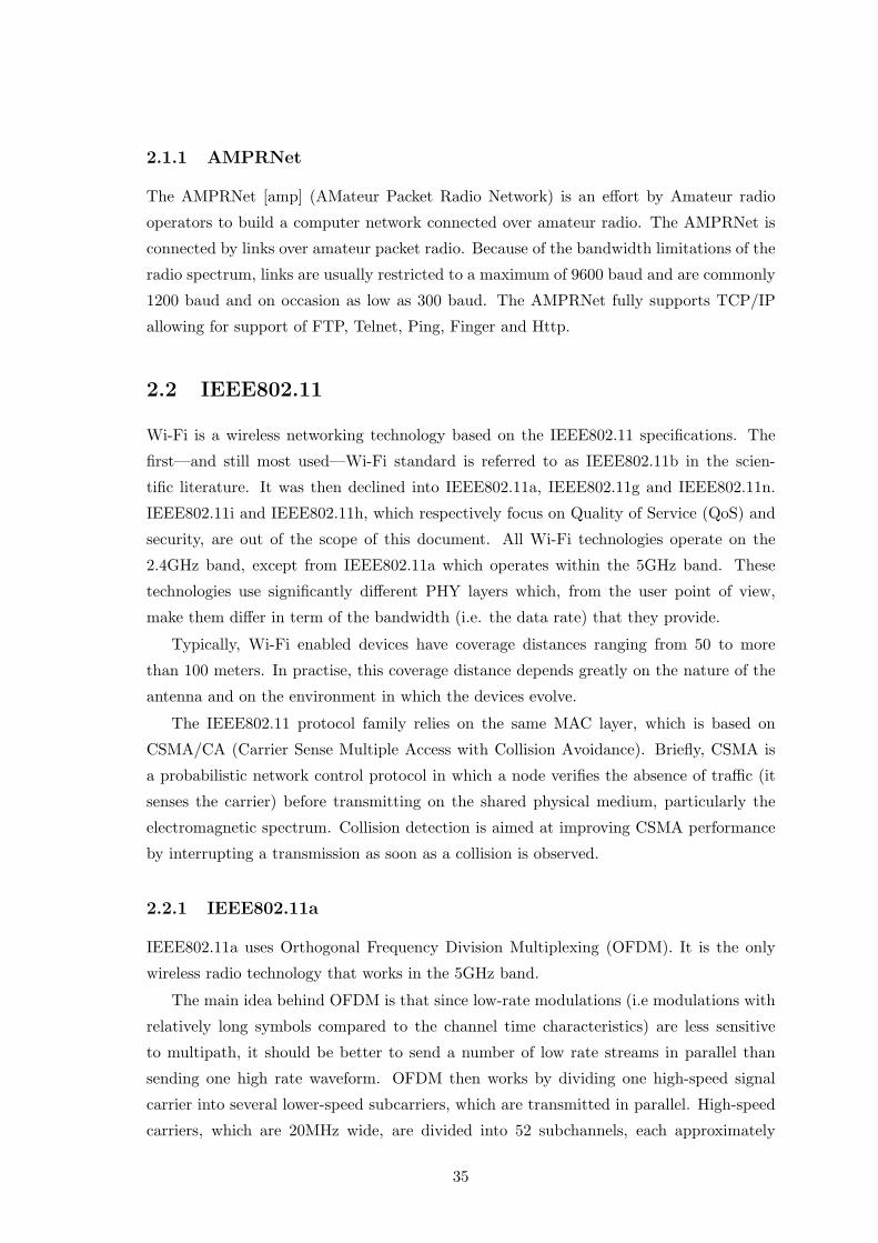
This document presents, in last chapter, the Delay Flooding with Cumulative Neigh-
borhood (DFCN) protocol [?, HBG+06]. DFCN is a broadcast protocol which achieves
performances comparable to SBA and AHBP, but that content with 1-hop neighborhood
information.
21

22

Contributions
The contribution of my work is mostly twofold. Briefly, it consists of (1) a mobile ad
hoc network simulator and (2) a versatile broadcasting protocol. Details are given in the
following.
First, my investigation of mobile ad hoc networking started with the study of broad-
casting protocols for large-scale metropolitan ad hoc networks. This requires a simulation
tools that enables to instantiate large amount of nodes. It also requires the ability to sim-
ulate heterogenous networks as well as to make the nodes move similarly to the way people
move in reality. At the best of my knowledge, when this research started (mid-2003) none
of the simulators available were proposing all of these features in a single package. Thus,
the development of the Madhoc simulator was motivated by both the need to have a
tool specifically tailored to my purposes and by the will to explore the profound details of
the wireless communication paradigm. Briefly, Madhoc provides a lightweight simulation
engine for the simulation of large numbers of nodes as well as a mobility model which
reproduces some properties of the citizen mobility. Additionally, Madhoc provides its
user with a graphical user interface which allows the precise monitoring of the simulation
processes at the moment is it running.
Second, after a survey of the broadcasting protocols suited to mobile ad hoc network-
ing, we found out that no truly efficient protocols operated both with 1-hop neighborhood
information and when the network is sparse. Delayed Flooding with Cumulative Neighbor-
hood (DFCN) was build with these two constraints in mind. Through experimentations,
DFCN exhibited the expected results, not to say better ones. On the one hand the strat-
egy it employs makes that DFCN keeps working even when the node density is extremely
low (very sparse network). On the other hand, when the density is high enough the state-
of-the-art protocols have shown that they work well, DFCN exhibits lower bandwidth
utilization. A counterpart of these good results, is that DFCN does not ensure that all
the nodes in the network will be reached. But anyway, in a mobile ad hoc network, even
protocols which theoretically ensure that all nodes will be reached will actually reach all
the nodes belonging to the partition in which the broadcasting process has begun—and
these protocols do not ensure that this partition includes all the nodes in the network.
23

24

Part I
Ad hoc networking: generalities
25

According to recent studies by Point Topic 3and DSL Forum4, the ration of the popu-
lation having an Internet access at home has increased at the astonishing rate of 40% per
year since 2000. In addition to this, more and more commercial toolkits for Internet access
propose a wireless networking adapter. At the same time, personal communicating devices
—like PDAs, mobile phones, multimedia players, gaming consoles, etc— are becoming part
of our daily life. For instance, the spreading ratio of mobile phones is close to 100% in
most western European and Northern American regions. Moreover, next generations of
such devices will likely come with Wi-Fi interfaces. Many mobile phones are already able
to communicate using Wi-Fi or Bluetooth, and provide features generally found in PDAs,
multimedia players or gaming consoles. This general tendency leads us to envision a future
in which most people will be equipped with devices able to communicate using wireless
interfaces.
In a wireless network the nodes communicate by sending and receiving electro-magnetic
(radio) waves. Wi-Fi networks —which are wireless networks that use the Wi-Fi technology
for data encoding— can operate in two modes, named “infrastructure” and “ad hoc”. On
the one hand, in infrastructure mode, the communication relies on some access point.
This access point rules the behavior of the local wireless network (WirelessLAN). Most
often, the access point also allows the nodes in the WirelessLAN to access nodes outside
of it. In particular this provides access to the Internet. The infrastructure mode is most
commonly used, and is used to enable access to the Internet in public places such as
train stations, airports, companies, and at home. On the second hand, in ad hoc mode,
nodes communication occurs in a peer-to-peer manner. In this case no infrastructure is
required. This mode presents the great advantage that communications do not require
any infrastructure. Hence ad hoc networks are cheap and robust. Unfortunately they
face a number of issues that still prevent their deployment. In particular, the technology
still needs to gain more maturity, and ad hoc applications are still a topic of research: so
far, gaming, sensing and military applications constitute the main applications of ad hoc
networks. All along this document, the focus will be put on mobile ad hoc networks, as
defined in the following.
Mobile ad hoc networks are wireless networks built on-the-fly by mobile computers (also
called “nodes”, “terminals” or “stations”) getting in and out of range with each others. In
mobile ad hoc networking, “radio communication” and “mobility” are key aspects. On the
one hand, nodes have limited radio range, which implies that they can communicate only if
they are close to each other—if they are in range. This requirement is not enough however.
Wireless communication have a number of issues which lead to situations in which two
nodes in range cannot communicate because the communication fails or because they do
3http://point-topic.com/4http://www.dslforum.org/
26

not detect each other. On the other hand, node mobility heavily impacts the connectivity
of the network. Mobility leads to network specific topologies and dynamic properties.
For example, if the nodes move in a random manner, the connection cannot be assumed
durable. Another example, if the nodes move in groups, then it is likely that cluster will
appear. In such situations, the current implementations of common network operations
like broadcast, unicast, routing, are not operable. Researchers steadily propose solutions
for enabling these basic operations in mobile ad hoc networks.
All along this document, we will consider a subclass of mobile ad hoc networks, called
delay tolerant networks. One of the most prominent properties of delay tolerant networks
are a high and unpredictable mobility and disruption of the network connections.
There exist a number of technologies which enable mobile ad hoc networking. The
most popular one is IEEE802.11, used in ad hoc mode. IEEE802.11 is commonly referred
to as “Wi-Fi”. Less frequently encountered, Bluetooth is becoming popular in the context
of Personal Area Networking (PAN). However its design apparently suits better mobile ad
hoc networking. Protocols such as Hiperlan, ZigBee, etc, provide alternatives solutions to
mobile ad hoc networking but, up to now, they sort of failed at attracting the attention
of the research groups. As of writing, most articles published on the topic of mobile ad
hoc networking present experiments based on IEEE802.11. Mobile ad hoc networking
is today is a vast area of research which gathers researchers working on the topics of
networking, distributed systems, complex systems, security, telecommunications, etc. In
the future, when mobile ad hoc networks will be deployed at a real scale, they will allow
the deployment of applications such as e-commerce, conferencing, gaming, mobile grid
computing applications, etc.
This chapter provides some definitions of what is a mobile ad hoc network, in Section 1.
Then, in Section 2 it gives some technical details on the wireless networking technologies
that are available today, and that suit the deployment of a mobile ad hoc networks. Finally,
in Section 3 it presents some applications which are likely to be deployed over the future
mobile ad hoc networks.
27

Chapter 1
Definition for “ad hoc network”
Ad hoc networks are gaining more and more interest. Not only their importance in military
applications [BZG04] is growing, but also their future impact on business is becoming clear.
Indeed the wide spread of lightweight and low-cost mobile devices—mobile phones, PDAs,
Pocket PCs, etc—which now embed Bluetooth and IEEE802.11 (Wi-Fi) network adapters
enable the spontaneous creation of city-wide mobile ad hoc networks. These networks could
then constitute the infrastructure of numerous applications such as emergency and health-
care systems [KGSMG02], groupware [BLH01], gaming [RTVS03, GFH05, RWW03], ad-
vertisements, customer-to-customer applications (like the UbiBay project [FLS02]), etc.
A prime issue when dealing with ad hoc networks certainly is to define what it is.
Indeed, there is no consistency in the literature about the definition of an ad hoc network.
The large variety of wireless networks—ranging from city mesh networks to sensor networks
[ASSC02]—makes it difficult to get a clear picture of the topic. What brings some more
difficulty is the gap between what is it possible to do today and what will be possible in
the future. For instance, as of 2006, building an ad hoc network is not an easy task. Even
if the technology exists, there still are a number of issues which makes the deployment of
a multi-hop ad hoc network a very challenging task.
In the coming sections are given and detailed a variety of the definitions found in the
literature. The reason for choosing these definitions is that they prove complementary.
Altogether, they provide a fairly good picture of what ad hoc networking is.
1.1 Definitions from the literature
From the etymological point of view, the term “ad hoc” is a Latin adjective which has two
possible substances, as given by Wordnet [Fel98]:
1. concerned with one specific purpose ;
2. improvised.
28

The term “ad hoc” were borrowed some time ago by computer scientists who extended
its meaning to characterize a network—or a connection—involving wireless devices. The
etymology for “ad hoc” suggests that an ad hoc network would be a network made of a
set of nodes collaborating to achieve a common goal. Further, the reason for being of an
ad hoc network IS this common goal. But in reality ad hoc networking is not primarily
about collaboration. Unfortunately, this has led to the use of confusing definitions.
Surprisingly, even if the concept of “ad hoc network” is clear to researchers, none of the
definitions proposed by researchers got universally accepted. Instead, a wealth of them
are in use in the literature.
1.1.1 IEEE802.11 specification
According to the IEEE802.11 specification [ANS99]:
Definition — “An ad hoc network is a network composed solely of stations
within mutual communication range of each other via the wireless medium.”
This definition implies that an ad hoc network is a complete one, in the sense that
all stations are in the neighborhood of each others. Among the consequences, an ad hoc
network is necessarily single-hop; it cannot be partitioned; and the mobility of the stations
has no impact on the network topology. Our understanding goes far beyond this mere
definition, as detailed in Section 1.2.
1.1.2 Stojmenovic and Wu
According to [SW04],
Definition — “wireless networks consist of static or mobile hosts (or nodes) that
can communicate with each other over the wireless links without any static network
interaction. Each mobile host has the capability to communicate directly with
other mobile hosts in its vicinity. They can also forward packets destined for other
nodes. Examples of such networks are ad hoc, local area, packet radio, and sensor
networks, which are used in disaster rescues, wireless conferences in the hall,
battlefields, monitoring objects in a possibly remote or dangerous environment,
wireless Internet etc.”.
This definition precisely defines what is a pure ad hoc network. In such a network,
no wireless access point is used and the nodes rely on themselves (and on their peers)
to established the communication links within the network. Note that this allows the
presence of static nodes. This implies that if the ratio of static nodes in the network is
high, they could act altogether as a set of access points. This would be contrary to the
definition.
29

1.1.3 Bhaskar
[BR03] does not leave out the eventuality that a mobile ad hoc network includes some
wired connections.
Definition — “Essentially a mobile ad hoc network is a collection of mobile
nodes communicating over wireless channels with little (if any at all) fixed, wired
infrastructure.”
More generally, close to Bhaskar’s definition, many researchers consider that it is always
possible to set up some—even minimal—infrastructure prior to the deployment of an ad
hoc network. Because mobility and wires are two components that do not mate well,
this infrastructure can be made of a set of wireless access points, or even one single long-
range one, located in the middle of the network. One might think that the use of some
infrastructure solves most of the issues inherent to ad hoc networking. But since this does
not mean that all the nodes are connected to the infrastructure, solutions (like the use of
central services) are not practicable.
1.1.4 Gerla
According to [GLR05]:
Definition — “A mobile ad hoc network (mobile ad hoc network) is a collection
of mobile nodes that dynamically self organize in a wireless network without using
any pre-existing infrastructure. In a MANET, the applications are typically “peer-
to-peer” rather than “client-server”. Moreover, a MANET is often built to support
a specific application, thus the networking is application-driven.”
This definition highlights two relevant things.
First, self-organization is an important concept of ad hoc networking. It is a generic
term that appears at several levels. Mostly it refers to routing: flat (in opposite to hierar-
chical) ad hoc architectures are not scalable. In order to overcome this major drawback,
hierarchical routing is introduced. The main challenge in hierarchical routing is to group
nodes into clusters, each cluster being represented by one cluster head. Self-organization
is also mentioned when dealing with topology control issues. In this context, the nodes
of the network move and alter the strength of the radio signal they emit so that they
collaboratively work at improving the connectivity of the network (that is reducing the
number of partitions as well as the shortest path length).
Second, the concept of application is to be discussed. Due to the particular character-
istics of ad hoc networks, not all distributed applications can be adapted to execute on
30

them. For example, because they are intrinsically highly dynamic, only loosely distributed
applications are possible. More details on applications for ad hoc networks are described
in Section 3.
1.1.5 MobileMANs
Metropolitan ad hoc networks are spontaneous wireless network resulting of the radio in-
teractions of the citizen’s mobile devices. Up to now, few groups have studied metropolitan
ad hoc networks. At the best of our knowledge, the most advanced research is conducted
in the frame of the MobileMAN project [CGMT03]. The following definition is adapted
from the MobileMAN project description:
Definition — A MobileMAN is a wireless mobile ad hoc network built up
solely from citizen devices. As such, it is autonomous and self-organized. The
kind of devices that populate MobileMANs are mobile phones, Personal Digital
Assistants (PDAs) equipped with wireless interfaces and, to a lesser extent, mobile
computers. Except from mobile computers, such devices are (relatively) low cost,
and operate without per-use service fees. The only external resource needed for
operation is the bandwidth in the (unlicensed) industrial, scientific and medical
(ISM) band. The devices forming a MobileMAN must cooperatively provide some
services such as naming, security, service discovery, etc. These services are needed
to support user-level applications.
Applications supported by a MobileMAN might range from text messaging systems,
up to more demanding multimedia (voice and video) services. Eventually, they might even
range from simple interactive games to ones that truly merge real, and virtual worlds.
MobileMANs are very likely to be the sort of ad hoc networks that will be most
frequently encountered in the future.
Because of the variety of configurations which compose a city, the topology of Mo-
bileMANs is heterogeneous; that is MobileMANs exhibit areas whose the concentration
of nodes ranges from highly dense to very sparse. Analogously, the mobility of the nodes
within a MobileMAN is complex: some nodes move in groups, some others do it in an
independent manner; some move fast, some other move slowly, etc. This characteristics
constitute obstacle to the execution of (distributed) applications for MobileMANs.
1.1.6 Delay Tolerant Networks
Delay tolerant networks (DTNs) [Fal03, JFP04, JLW05] constitute an emerging subclass
of mobile ad hoc networks that feature frequent and long-duration partitions. Indeed,
under some particular conditions like fast mobility or poor connectivity, the topology of
31

the network is steadily affected, leading to low densities. In a delay tolerant network, the
disruption of connections is not considered to be a situation of error, instead it constitute
a normal behavior of the system. Consequently there must be a software layer which take
into account this prominent property of delay tolerant networking.
DTNs have a variety of applications like Vehicular Ad hoc Networks (VANETs) [TMJH04],
sensor networks [ASSC02], military networks, etc.
All along this document, the term “mobile ad hoc network” will be mostly referring to
delay tolerant networks.
1.2 Synthetic definition
On the basis of the previous definitions and the literature on the topic, in the rest of this
document, the following synthetic definition will be assumed:
Definition — A mobile ad hoc network (also referred to as mobile ad hoc net-
work) is a collection of communication nodes which are generally mobile. The
nodes may be of different natures (mobile phones, laptops, PDAs, wearable de-
vices, workstations, etc).
The network connections the nodes use to communicate cannot be assumed reli-
able (because of node motion, connections might break down at any time). They
may be of various types (Wi-Fi, Bluetooth, Ethernet, etc).
The network resulting of the interaction of the nodes exhibits a topology that is
generally not predictable. It operates in a complete peer-2-peer manner, that is
node-to-node communication do not rely on any network infrastructure. Instead
nodes establish direct communications with their peer nodes, hence peer-to-peer.
In this document we will use the term “pure ad hoc network” for referring to ad hoc
networks whose the connections are all peer-to-peer. In other words, an ad hoc network in
which at least one connection connects a node to a fixed infrastructure will not be referred
to as “pure”.
Often in this document we will refer to the neighborhood of a node.
Definition — A node a is a neighbor of a node b if there exists a network link
that directly interconnects a and b. The neighborhood of a given node is then
the set of nodes which are neighbors of this node.
This definition implicitly considers the nodes which are “direct” neighbors of a given
node. But the concept of neighborhood can be broaden, as given by the following definition:
32

Definition — A node a is said to be at n hops of a node b if there exists a path
from a to b which is established by n− 1 intermediate different nodes.
The n-hop neighborhood of a given node then is the set of nodes which are at
n-hops of this node.
33

Chapter 2
Ad hoc networking technologies
Theoretical mobile ad hoc networking research [CCL03] started some decades ago. But
commercial digital radio technologies appeared in the mid-nineties. Since then, few pro-
posal for enabling ad hoc communications were made. The first technology (IEEE802.11,
also referred to as Wi-Fi [ANS99]) is still strongly leading the market, although there is
great room for improvement. This section provides an overview and a technical description
of the technologies that have been proposed hitherto.
A common feature of most wireless networking technologies is that they operate in the
unlicensed Industrial Scientific and Medical (ISM) 2.4GHz band. Because of this choice
of frequency band, the network can suffer interferences from microwave ovens, cordless
telephones, and other appliances using this same band plus, of cours, other networks. In
particular, Farrell and Abukharis studied the impact on Bluetooth on IEEE802.11g [ST04]
2.1 Packet radio
Packet radio [GFS78] was used for the earliest versions of mobile ad hoc networks. It
was sponsored by DARPA in the 1970s. It allows the transmission of digital data over
amateur radio channels. Using special radio equipment, packet radio networks allowing
transmissions at 19.2 kbit/s, 56 kbit/s, and even 1.2 Mbit/s have been developed.
Since the modems employed vary in the modulation techniques they use, there is no
standard for the physical layer of packet radio networks. Packet radio networks use the
AX.25 data link layer protocol, derived from the X.25 protocol suite and designed for
amateur radio use. AX.25 has most frequently been used to establish direct, point-to-
point links between packet radio stations, without any additional network layers.
However, in order to provide routing services, several network layer protocols have
been developed for use with AX.25. Most prominent among these are NET/ROM, ROSE,
and TexNet. In principle, any network layer protocol may be used, including the Internet
protocol (IP), which was implemented in the framework of the AMPRNet project.
34
2.1.1 AMPRNet
The AMPRNet [amp] (AMateur Packet Radio Network) is an effort by Amateur radio
operators to build a computer network connected over amateur radio. The AMPRNet is
connected by links over amateur packet radio. Because of the bandwidth limitations of the
radio spectrum, links are usually restricted to a maximum of 9600 baud and are commonly
1200 baud and on occasion as low as 300 baud. The AMPRNet fully supports TCP/IP
allowing for support of FTP, Telnet, Ping, Finger and Http.
2.2 IEEE802.11
Wi-Fi is a wireless networking technology based on the IEEE802.11 specifications. The
first—and still most used—Wi-Fi standard is referred to as IEEE802.11b in the scien-
tific literature. It was then declined into IEEE802.11a, IEEE802.11g and IEEE802.11n.
IEEE802.11i and IEEE802.11h, which respectively focus on Quality of Service (QoS) and
security, are out of the scope of this document. All Wi-Fi technologies operate on the
2.4GHz band, except from IEEE802.11a which operates within the 5GHz band. These
technologies use significantly different PHY layers which, from the user point of view,
make them differ in term of the bandwidth (i.e. the data rate) that they provide.
Typically, Wi-Fi enabled devices have coverage distances ranging from 50 to more
than 100 meters. In practise, this coverage distance depends greatly on the nature of the
antenna and on the environment in which the devices evolve.
The IEEE802.11 protocol family relies on the same MAC layer, which is based on
CSMA/CA (Carrier Sense Multiple Access with Collision Avoidance). Briefly, CSMA is
a probabilistic network control protocol in which a node verifies the absence of traffic (it
senses the carrier) before transmitting on the shared physical medium, particularly the
electromagnetic spectrum. Collision detection is aimed at improving CSMA performance
by interrupting a transmission as soon as a collision is observed.
2.2.1 IEEE802.11a
IEEE802.11a uses Orthogonal Frequency Division Multiplexing (OFDM). It is the only
wireless radio technology that works in the 5GHz band.
The main idea behind OFDM is that since low-rate modulations (i.e modulations with
relatively long symbols compared to the channel time characteristics) are less sensitive
to multipath, it should be better to send a number of low rate streams in parallel than
sending one high rate waveform. OFDM then works by dividing one high-speed signal
carrier into several lower-speed subcarriers, which are transmitted in parallel. High-speed
carriers, which are 20MHz wide, are divided into 52 subchannels, each approximately
35

300KHz wide. OFDM uses 48 of these subchannels for transporting data, while the four
others are used for error correction.
OFDM delivers higher data rates and a high degree of multipath reflection reconstruc-
tion, thanks to its encoding scheme and error correction. The IEEE802.11a standard
permits the data rate to be set at 24 Mbit/s. But it also allows vendors to extend it
beyond that. However, the more bits per cycle (Hz) that are encoded, the more fragile the
signal will be to interference and fading, and unless power output is increased, the shorter
the range.
In practise, vendors typically sell IEEE802.11a devices that boast data rates up to 54
Mbit/s.
2.2.2 IEEE802.11b
IEEE 802.11b uses Direct Sequence Spread Spectrum (DSSS) as the physical layer tech-
nique for the standard.
DSSS uses a complex technique which consists in multiplying the data being transmit-
ted by a noise signal. This noise signal is a pseudo-random sequence of 1 and −1 values,
at a frequency much higher than the original signal.
The resulting signal wave looks much like white noise. This white noise can be filtered
at the receiving end in order to recover the original data. This filtering happens by again
multiplying the same pseudo-random sequence by the received signal (because 1× 1 = 1,
and −1 × −1 = 1). This process, known as “de-spreading”, mathematically constitutes
a correlation of the transmitted pseudo-random sequence with the receiver’s assumed se-
quence. For allowing de-spreading to work correctly, the transmit and received sequences
must synchronized.
So far, IEEE 802.11b is the implementation of the IEEE 802.11 standard that has been
most heavily studied in the framework of mobile ad hoc networks.
2.2.3 IEEE802.11g
IEEE802.11g, just like IEEE802.11a, uses Orthogonal frequency-division multiplexing (OFDM),
it then boasts similar bandwidths. OFDM is described in Section 2.2.1. But unlike
IEEE802.11a, IEEE802.11g works in the 2.4 GHz band.
Since the draft 802.11g standard combines fundamental features from both 802.11a and
802.11b, it leads to the development of devices that can inter-operate with technologies
based on both of the previous versions of the specification.
36

2.2.4 IEEE802.11n
IEEE802.11n [dMSGLA06] is built on previous 802.11 standards by adding MIMO (multiple-
input multiple-output). MIMO uses multiple transmitter and receiver antennas to allow
increased data throughput and range.
2.3 Bluetooth
Bluetooth is essentially the same kind of microwave radio technology that has given us
wireless door chimes and automatic garage door openers. It was initially restricted to an
operating distance of just 10 meters and a speed of approximately 1 Mbit/s.
When Bluetooth devices come within range of each other, they establish contact and
form a temporary network called a Personal Area Network (PAN). In the Bluetooth ter-
minology, this is also known as a Piconet. A multi-hop ad hoc network formed by the
interaction of Bluetooth devices is called a Scatternet. When using Bluetooth, the devices
must establish a network session before being able to transmit any data.
Bluetooth uses the Frequency-Hopping Spread Spectrum (FHSS) technique. Unlike
IEEE802.11 which establishes a communication link on a certain frequency (a channel),
FHSS breaks the data down into small packets and transfers it on a wide range of fre-
quencies across the available frequency band. Bluetooth transceivers jump among 79 hop
frequencies in the 2.4 GHz band at the rate of 1,600 frequency hops per second. 10 differ-
ent types of hopping sequences are defined, 5 of the 79 MHz range/79 hop system and 5
for the 23 MHz range/23 hop system. This technique trades off bandwidth, in order to be
robust and secure. More precisely, Spread Spectrum communication techniques have been
used for many years by the military because of their security capabilities.
Thanks to this, Bluetooth allows the transmission of data as well as voice (VoIP ap-
plications).
2.4 Hiperlan
The HiperLAN2 standard is very close to 802.11a/g in terms of the physical layers it
uses—both use OFDM technology—but is very different at the MAC level and in the way
the data packets are formed and devices are addressed. On a technical level, whereas
802.11a/g can be viewed as true wireless Ethernet, HiperLAN2 is more similar to wireless
Asynchronous Transfer Mode (ATM). It operates by sharing the 20MHz channels in the
5GHz spectrum in time, using Time Division Multiple Access (TDMA) to provide QoS
through ATM-like mechanisms.
It supports two basic modes of operation: centralized mode and direct mode. The cen-
tralized mode is used in the cellular networking topology where each radio cell is controlled
37

by an access point covering a certain geographical area. The direct mode is used in the
ad hoc networking topology - mainly in the context of Personal Area Networking - where
a radio cell covers the whole serving area. In this mode, mobile terminals in a single-cell
home “network” can directly exchange data.
HiperLAN2 support came mainly from European telecommunications equipment ven-
dors.
2.5 BLAST
Announced in 1998, BLAST [GDG98], which stands for Bell Labs Layered Space-Time, is a
wireless communication technique which uses multi-element antennas at both transmitter
and receiver. BLAST boasts bandwidth eight times bigger than conventional approaches.
The BLAST project does no longer show clear signs of activity, since the last related
publications date from 2002. IEEE802.11n (see section 2.2.4) uses the same principle.
2.6 ZigBee
ZigBee-enabled devices conform to the IEEE 802.15.4-2003 standard. This standard spec-
ifies its lower protocol layers, the physical layer (PHY), and the medium access control
(MAC). It targets Low-Rate Wireless Personal Area Network (WPAN). ZigBee-style net-
works research began in 1998. Zigbee was intended to operate in contexts in which both
Wi-Fi and Bluetooth are not suitable.
Zigbee operates in the unlicensed 2.4 GHz, 915 MHz and 868 MHz ISM bands. It
uses direct-sequence spread spectrum (DSSS) coding. This makes the data rate to reach
250 kbit/s per channel in the 2.4 GHz band, 40 kbit/s per channel in the 915 MHz band,
and 20 kbit/s in the 868 MHz band. The maximum output power of ZigBee antennas
being generally 1 mW, the transmission range of ZigBee nodes is between 10 and 75
meters. Observations have shown that the transmission range is heavily dependent on the
environment.
The MAC layer specified by IEEE 802.15.4-2003 is CSMA/CA (carrier sense, multiple
access/collision avoidance).
2.7 Broadband wireless networking
WiMAX (IEEE 802.16) stands for Worldwide Interoperability for Microwave Access. IEEE
802.16 boasts data rates up to 70 Mbit/s over a distance of 50 km. However practical limits
from real world tests seem to be between 500 kbit/s and 2 Mbit/s at a distance of around
5-8kms.
38

WiBro is a wireless broadband internet technology being developed by the Korean
telecoms industry. It has been announced that WiBro base stations will offer an aggregate
data throughput of 30 to 50 Mbit/s and cover a radius of up to 5 km. The technology will
also offer Quality of Service.
HIPERMAN [HPF03, HPF04], which stands for High Performance Radio Metropolitan
Area Network, is a European alternative to WiMAX. The standard were created by the
European Telecommunications Standards Institute (ETSI). It provides a wireless network
communication in the 2-11 GHz bands.
The adequation of these technologies to ad hoc networking is discussable, since they
would permit to establish ad hoc networking at a level at which technologies for infras-
tructured networks (like GSM or UMTS) are available.
2.8 Adequation to ad hoc networking and issues
Not all of the protocols described hereinbefore were initially designed for enabling ad hoc
networking. More precisely most of the effort on Wi-Fi (IEEE802.11) aimed at enabling
wireless local area networking (WLAN). In this context, IEEE802.11 works nicely. When
used in ad hoc mode, it proves to be barely utilizable. Bluetooth were primarily designed
and implemented for enabling Wireless Personal Area Networking (WPAN). A WPAN
is a network used for communication among computer devices (including telephones and
personal digital assistants) close to one person. In this context Bluetooth competes stan-
dards such as the wireless WUSB (Wireless Univeral Serial Bus, technically referred to as
IEEE802.15.3) and IrDA (Infrared Data Association), and the wired USB and Firewire
(IEEE 1394).
2.8.1 Synchronization issue
Used in ad hoc mode, IEEE802.11b (section 2.2.2), and more generally the Direct Sequence
Spread Spectrum (DSSS) physical-layer technique, suffers from several problems that make
it hardly usable. In particular, the time synchronization techniques used by DSSS for de-
spreading the frame received constitute a strong constraint at the level node discovery.
For example, let us consider the simple case of four nodes a, b, c, d, a being in sync with
b, and c in sync with d. c moves in the direction of b. When c arrives in the vicinity
of b, none of them may emit beacons —nor listen to incoming ones— because they may
be synchronized on d and a, respectively. In such a situation b and c would be perfectly
unable to detect their new geographical neighbor. Figure 2.1 illustrates this.
This is an issue since it hardly impedes the creation of multi-hop ad hoc networks.
39

a
b
d
c
Figure 2.1: b and c are unable to detect one another because they do not emit nor receive
beacons.
2.8.2 Latency of the discovery
When two given nodes get in range, if there is no synchronization issue, they should be
capable to detect the presence of each other. The duration of this discovery process is
sometimes an issue.
Using IEEE802.11b-enabled devices, the discovery is reasonably fast if at least one of
the two nodes is emitting a beacon frame. The node that is not emitting any beacon frame
(or whose the clock is set backward) will synchronize to the other nodes’ clock. Since ten
beacon frames are sent during one second, the discovery of a new node lasts at most one
tenth of a second plus the time needed to perform the synchronization and to establish
the link. This generally lasts less than a second. As explained in Section 2.2.2, if both
nodes previously received beacons frame from other nodes, they have turned to passive,
thus they are not emitting any beacon. Consequently they are not visible and have no
chance to discover each other.
Using Bluetooth, two mechanisms are at issue. On the one hand, the time required
by Bluetooth module to scan the carrier for new neighbor takes a few seconds. In the
case of mobile nodes, this is an issue: since the diameter of coverage area of Bluetooth
nodes do not generally exceed twenty meters, a module moving faster than 6 m/s (roughly
the speed of a bicycle) crosses the coverage area of another module in at best 3 seconds.
Which is too short to allow detection. Bluetooth as its works now it then now suitable
for highly dynamic ad hoc networks. On the other hand, because Bluetooth modules use
only 3-bit MAC addresses, Bluetooth piconets (that is how Bluetooth ad hoc networks are
called) cannot gather more than 8 devices (1 master and 7 slaves). Moreover, Bluetooth
scatternets are not well-developed today. Most researchers have focused on theoretical
40

concepts. Some algorithms for scatternet formation were proposed [CMA04], on the basis
of simulations. The BTnode project [BKM+04], conducted at ETH Zurich, is one of the
first actual implementations of Bluetooth scatternets.
41

Chapter 3
Target applications
Mobile ad hoc networks are mostly used today for physical sensing (temperature, pressure,
etc) and for military applications. Their probable deployment in the near future will make
them a new execution platform for many distributed applications. But because of their in-
trinsically highly dynamic nature, mobile ad hoc network will likely serve as the execution
support of loosely distributed applications. In the coming subsections are describe some
applications that should be executable on a mobile ad hoc network. Indeed distributed ap-
plication whose the components are tightly coupled do not support connection disruption.
For example, in the case of a J2EE three-tiers distributed application, when the database
gets disconnected from the application server, the whole application gets out of order.
3.1 Vehicular ad hoc networks
Vehicular Ad hoc Networks (VANETs) [TMJH04] represent one of the most promising
civil application scenarios for ad hoc networking since it already constitutes a business
involving several big companies like XEROX, BMW and many others.
VANETs rely on two approaches:
• Inter-Vehicle Communication (IVC). In this approach, all vehicles behave equally.
They are connected to each others (in accordance to their distance) so that they
constitute a pure ad hoc network.
• Roadside-to-Vehicle Communication (RVC). In that approach, access points are in-
stalled on the roadside. Located regularly, they constitute a backbone to the vehicu-
lar wireless network. However, although it is made of mobile entities communicating
via the wireless link such a network could not be be qualified as ad hoc.
VANETs will help to avoid crash situations but also significantly improve the comfort
and efficiency of driving with respect to time and energy. Further, they can also be used
for reducing traffic congestion and for enabling automatic driving.
42

VANETs exhibit an issue which seems to have apparently not been tackled up to now:
there exists a threshold in how relatively fast (emitting and receiving) nodes move above
which the receiver are no longer capable to demodulate the incoming signal. For instance,
Hiperlan is announced to feature a tolerance to mobility which is about 10m/s, meaning
that two nodes moving at a relative speed greater than about 35km/h would not be able to
communicate. This upper-bound limit might pose problems in the context of VANETs.
3.2 Sensing
A wireless sensor network [ASSC02] is a computer network consisting of many, spatially
distributed devices which embed sensors to monitor conditions at different locations, such
as temperature, sound, vibration, pressure, motion, etc. Sometimes these devices are small
and inexpensive, so that they can be produced and deployed in large numbers. The size and
price requirements implies that their resources in terms of energy, memory, computational
speed and bandwidth are severely constrained. Each device is equipped with a radio
transceiver, a small micro-controller, and an energy source, usually a battery. Each device
relays information from other devices to transport data to a monitoring computer.
[DM05] states that sensor networks actually are ad hoc networks, but mobility is ab-
solutely not central to ad hoc networks. As a matter of fact, most sensor networks are
made of immobile sensor, strategically located so as the collaborative measurement sys-
tem is appropriate. But in some case sensors are deployed in mobile terrain. For example
there exist sensors which are meant to study the behavior of tornados. Then hundred of
them are carried by the wind and report location, speed and pressure measures. In such a
case of a sensor network, mobility is key. Applications of sensor networks include environ-
mental and medical monitoring, seismic Detection, habitat monitoring, acoustic detection,
military surveillance, etc.
3.3 Personal area networking
A personal area network (PAN) is a network used for communication of computer devices
close to one person. Those devices include mobile phones, personal digital assistants,
home computer, audio systems, etc. The coverage range required is generally of a few
meters. PANs can be used for ad hoc communication among the devices themselves or for
connecting to a backbone network like the Internet.
Up to now, personal area networks have been wired, relying on technologies such
as USB and FireWire. In the past years, IrDA and Bluetooth became of common use.
Efforts to turn Wi-Fi to a PAN technology have already started and Wi-Fi enabled devices
(typically printers, video cameras) can be found on the public market.
43

3.4 Military systems
Military applications are one of the most often described applications of mobile ad hoc
networks. Unfortunately, since military projects are discrete—if not secret—few informa-
tion is available. One of the main objectives of the militaries is to be able to deploy digital
networks on difficult terrains— terrains on which it is not possible to install any infras-
tructure prior to the arrival of the soldiers. For example, such a digital network would
allow soldiers to continuously be aware of the location of their peers. Today soldiers com-
municate with their peers using analog communication techniques such as radio-frequence.
Using digital communication would allow them to exchange structured data such as maps
or pictures of the terrain.
Within a military ad hoc network, the soldier is the network node. In this context, one
of the main issues are to find strategies which ensure that the ad hoc network will remain
connected as soldiers move. This problem is known as topology control. Military ad hoc
networks also have a deep concern with security and reliability.
3.5 Peer-to-peer computing
The term grid computing [TL03, AvLM04], whose the ideas were brought together by Ian
Foster and Carl Kesselman, originated in the early 1990s. It is a metaphor for making
computer power as easy to access as an electric power grid.
More precisely, grid computing (or “metacomputing”) provides a model for solving
massive computational problems: it makes use of the CPU and storage resources of large
numbers of computers (generally desktop computers) seen by the application as a large
virtual one. Grid Computing focuses on supporting computations across clusters of com-
puters located in distinct administrative domains. It then aims at federating the resources
generally used for cluster computing (or distributed computing) [ANG01, ASG97] which
operates on one single set of nodes located at one spot. Grid computing is then mostly
concerned by inter-operability and security issues, while cluster computing is more con-
cerned by job-scheduling, load balancing, etc. Grids can be declined according to what
they aim at:
• Computational grids [FK00] which focuses primarily on computationally-intensive
operations, job-scheduling, (dynamic) load balancing, etc.
• Data grids [Old01, CFK+99] which focus on strategies maximizing the storage space
available and reliability, minimizing the latency of retrieval.
The most prominent project in grid computing is Globus [All]. Other projects include
Unicore, Legion [GWT97, ANG01, GWF+94].
44

The idea behind ad hoc grid computing is to use the massive computational power
provided by the huge amount of mobile devices for solving computationally hard problems.
A number of issues must be solved before in order to enable this.
• the high dynamic nature of mobile ad hoc network imposes that the distributed
components of the grid-application must be loosely coupled;
• because of the high likeliness of node mobility or link failure, some robust scheduling
strategies must be defined;
• an inter-operability mechanism has to be designed, in order to overcome the diversity
of the devices ;
• because the nodes do not belong to a single administrative entity, security is a prime
issue: the nodes have little knowledge of one another ; trusts mechanisms must then
be employed. In this context, the concept of “reputation” is promising.
3.6 Risk management
Emergency applications are of prime importance, for example, in the populated areas in
which lots of hazardous companies are present. This is particularly the case in certain
region where the chemical industrial areas are a few kilometers away (sometimes even
less) from densely populated areas. In such a context, it seems essential to be able to
provide the population with some information on the danger and instructions on what to
do, as fast as possible. Currently, such warning systems are achieved by the use of sirens
(sometimes hardly audible) evenly located in the populated areas. Another solution would
be the use of a citizen ad hoc network.
There would then be an emergency application (some sort of broadcasting protocol)
deployed on all the mobile devices (mobile phones, PDAs, etc) of the civilians. A company
facing an highly dangerous issue could trigger the dissemination of a“catastrophe message”.
Rapidly, relayed by the mobile devices of the citizen, such a message would be received
by almost everyone. The broadcasting of such a message would operate without any
consideration of the bandwidth utilized, since its importance would be much higher than
any other application.
3.7 Advertising
The implication of mobile ad hoc networks in e-business applications is not well described
in the literature. So far, only few applications considered it. This is the case of the UbiBay
project [FLS02], a decentralized auction system for mobile ad hoc networks.
45

The diffusion of small advertisements constitutes another interesting e-business ap-
plication. Given a metropolitan ad hoc network deployed at the level of a city (or a
large sub-set of it), it would be commercially relevant to be provided with the possibility
to broadcast advertisement messages across the network. Common broadcasting scheme
could not be applied in this context: commercial applications should leave most of the
bandwidth available to more important applications, such as emergency ones 3.6.
The principle of small-advertising over mobile ad hoc networks is as follows: a person
(the seller) willing to sell a good write a short description of it, and attaches to it his contact
information. The description—the small ad itself—is broadcasted over the network. In
order to restrict the propagation of the message, a maximum number of allowed hops is
specified in the message. Upon reception of the message, the recipient node decreases
this maximum number of hops. Then the message is candidate to forwarding only if the
number of hops is greater than zero. A person whose the mobile device has received a
small-ad is alerted by a sound or something similar. If this person (the buyer) wants to
acquire the advertised good, he might simply use the contact information embedded in the
message for reaching the seller.
46

Part II
Simulation
47

In the situation today, real mobile ad hoc networks are not yet developed at a city-scale,
conducting research on mobile ad hoc networks is achievable either by using experimenta-
tion networks (called “testbeds”) or by resorting to software simulation. In the literature,
it appears that most of the work today is done by using simulators. Indeed testbeds
have a number of drawbacks like their high cost, the difficulty to built one, the difficulty
of monitoring them, etc. These drawbacks still refrain research labs from building large
test-beds. The study of large-scale applications—which is our very concern herein—most
often opt for modelling and software simulation. Researchers can then follow two direc-
tions, depending on their needs: either using one of the simulators made available to the
community or developing a custom simulator tailored to their purpose.
The world of simulators is largely dominated by ns-2. ns was originally targeted at the
simulation of wired networks. Its subsequent versions, ns-2, came with an extension for
mobile ad hoc networks. ns-2 is open-source and provides an implementation for most of
the protocols for mobile ad hoc networking. Less popular, simulators like GloMoSim or
Qualnet have advantages like the possibility to distribute the simulation over a cluster of
workstation, or to provide commercial support.
Although there already is a good wealth of simulators available on the market, as mobile
ad hoc networking research evolves it appears that more and more research groups favor
the development of custom simulators. Among the limitations of the most popular wireless
network simulators are the inability to simulate heterogeneous networks (that is networks
consisting of several radio communication technologies like IEEE802.11b or Bluetooth),
the difficulty to simulate large networks (on sequential simulators like ns-2, a few hundred
nodes seems to be an upper limit) and the lack of realistic mobility models. Currently,
most of the work in the field of mobile ad hoc networking rely on randomized mobility
models, such as the so-called “Random waypoint mobility model” is the one which is most
commonly used. These drawbacks constitute as many challenges that will be considered
in the rest of this document.
My work takes place in the framework of several multi-national academic projects.
Each of them came with different requirements. In particular the SoNi project [Uni07]
(Luxembourg) which was the initial source of funds aims at providing a framework al-
lowing the prototyping of fresh network primitives as well as ad hoc applications, all
considering realistic network conditions.
In the context of the GraphStream project [AD07] (France), researchers were looking for
a tool permitting the study of mobile ad hoc networks seen as complex systems (systems
made of highly numerous autonomous entities working independently at the emergence of
a global behavior).
One of the issues tackled by The SARAH project (France) is the design of an experimenta-
tion platform for the study of Delay Tolerant Networks (DTNs). A key issues was then how
48

to couple a test-bed and a mobile ad hoc network simulation so that the test-bed would
be virtually expanded by the simulated network. More precisely, the researches had before
build a IEEE802.11b-based network of laptops. On top of this they have implemented a
groupware application for the dissemination of documents. One of the perspective was
then to extend the network (in terms of the number of nodes) in order to observe the
behavior of the application. Madhoc was then used at managing a number of “virtual”
nodes. A software bridge then enables real nodes to transparently interact with virtual
ones.
The ABBASMUS [Uni] project addresses the issue of topology control for ad hoc net-
works. More precisely it aims at providing new topology control schemes based on the use
of “injection points”—connections from the ad hoc nodes to some infrastructured network.
This project hence required a simulator allowing the representation of links.
Last, in the framework of studies on multi-objective optimization (MOO), researchers
at Malaga University needed a simulation tool permitting the optimization of broadcast
protocols. Using some results of one single simulation process as the value of the fitness
function for their MOO algorithms, the key issue was to use a simulator that would be able
to operate the simulation of one broadcasting process in less than a second, in average.
The diversity of the requirements formulated by our academic partners imposed the
development of a custom simulator, named Madhoc. Indeed no other simulator would
have permitted us to meet the needs.
Madhoc is characterizable in a number of ways. Maybe its more relevant aspects lie
in its hybrid simulation engine and its mobility models, as explained in the following.
The philosophy design of Madhoc is twofold. From a general perspective, Madhoc is
object-oriented. In particular, the application programming interface it exhibits is made
of classes and objects, as it is usual in software design. However, as often as possible,
Madhoc models things in a probabilistic way. In particular, the model for the physical
network layer makes use of statistics. Doing this lightens the simulation engine. This
provides Madhoc with the ability to efficiently simulate large population of nodes (up to
twenty thousands nodes on regular desktop computers). The use of statistics avoids Mad-
hoc to implement loads of complex low-level mechanisms that would have required a huge
computational power and long time to execute. Instead an statistic-based implementation
rely on a small set of equations that are executable in a short time.
Madhoc provides a set of mobility models which includes the ubiquitous random
waypoint and random walk mobility models. In addition to this, it provides a more
sophisticated mobility model aiming at reproducing some properties of the mobility of
humans. This mobility model is called the“human mobility model” (HMM). Briefly, HMM
considers that the environment in which the nodes evolve has a number of particular areas
(called “spots”) in which nodes tend to go and stay for some time. These areas may
49

represent shop, or traffic lights, for example. For the moment, a randomized decision
function rules the motion of the nodes which move from spot to spot, taking care at not
visiting twice the same spot.
This part of the present document focusing on ad hoc networking experimentation
tool. It is divided in two sections. It first presents in Chapter 4 a State of the Art
of the experimentation platforms for mobile ad hoc networking, which include testbeds
and simulators. Then Chapter 5 describes Madhoc, a simulation-based experimentation
environment targeting the simulation of city-scale ad hoc networks.
50

Chapter 4
State of the Art
The State of the Art presented in this chapter first briefly introduces in Section 4.1 mobile
ad hoc networking testbeds, by providing a list of remarkable ones, and by explaining the
pros and cons for the use of such networks. Then it provides in Section 4.2 a description
of the wireless network simulators available, indicating the criteria that should guide the
researchers in search of the simulator that will best meet his needs. In section 6.1 is given
an analysis of the mobility models that are commonly employed in the context of the
investigation of human mobility. Finally, Section 4.3 presents a list of the issues that are
encountered when dealing with mobile ad hoc network simulation, and section 4.4 consists
of the author’s point of view on how mobile ad hoc network simulation will/should change
in the future.
4.1 Testbeds
Definition — Testbeds are in-lab networks built and used by researchers. They
are dedicated to the experimentation of protocols and applications over mobile
ad hoc networks.
A survey of the existing testbeds is proposed by De and al. [DScC].
Typically, testbeds consists of devices communicating through the TCP/IP network
stack. Most research projects use testbeds to find out of how TCP/IP operate in the
context of ad hoc networking. Ultimately, they permit the development of extensions that
make TCP/IP work better. Aside to this research focusing on the possible applications of
the internet protocols to ad hoc networking, some projects are based on the assumption
that such protocols do not suit mobile ad hoc networking. These projects hence aim at
defining brand-new techniques for enabling single-hop (defining physical and data-links
layers, respectively referred to as PHY and MAC layers) and multi-hop communication
(which is vastly concerned by routing techniques, seated at the network layer). Such
projects include DoDWaN [GR04], described in Section 4.1.1.
51

4.1.1 Some testbeds
Among all existing testbeds, the following ones are remarkable because of the number of
devices they gather, or because of the nature of communication link they use.
• The APE project [LLN+02] experimented routing on 37 IEEE802.11 nodes. Numer-
ous participants were involved—particularly for moving the devices—which impacted
the high costs and difficulty of the experiments. APE was built by the department
of Computer Systems at Uppsala University (Sweden) and was partly funded by
Ericsson.
• The RoofNet project (MIT) [CACM03], conducted over the city of Cambridge (UK),
uses 40 IEEE802.11 nodes. It primarily aims at studying mesh networks but it is also
employed at investigating multi-hop routing on MANETs. Citizens can connect to
the Internet through the research network. The RoofNet project uses static nodes.
It hence does not deal with mobility issues.
• Focusing on multi-hop routing, Douglas and Raichle [KR01] used a MANET testbed
made of 8 IEEE802.11 nodes.
• Ritter and al. [RTVS03] built a Bluetooth network for experimenting gaming and
home automation. In order to have a global view of the network—which makes
monitoring it a lot easier—they used 300m-range EWM adapters. This testbed is
one of the rare projects that make use of the Bluetooth technology.
• The Ad Hoc City project [JHP+03] uses an mixed approach: both wired and wireless
stations are used. By covering in time and space the whole city of Seattle (Washing-
ton, USA), real information of nodes’ movements could be gathered. This testifies
the current trend towards realistic mobility models.
• the DoDWaN testbed is dynamically created by mobile devices joining a single-
hop network. The devices communicate with one another by using the IEEE802.11
MAC. DoDWaN takes into accounts the properties of the delay tolerant networks.
For example, in a document dissemination application, stations that are not present
when the document dissemination was initiated will receive it when they will get in
contact with stations that were present at that time.
4.1.2 Issues
On the one hand, testbeds allow the researchers to run experiments using the real devices.
While, as described in Section 4.3.1, accuracy of the experimentations is at issue when
dealing when simulators, testbeds always provide accurate response.
On the other hand, testbeds suffer from numerous drawbacks, as listed in the following:
52

• the number of devices they involve is limited: the cost of the hardware (one node is
several hundred euros) limits testbeds to few dozen nodes;
• the experimentations conducted on testbeds are not reproducible—reproducibility
being a prime feature of scientific experimentation;
• they are not scalable;
• the inherently distributed nature of ad hoc networks constitutes a great lack of flexi-
bility. More precisely, because the network cannot be handled as a whole, monitoring
is difficult. Because the network is made of several devices, deploying an application
implies a deployment on all devices.
• unless the devices are embedded on some sort of vehicle, they become mobile only if
someone is here to move them.
There have been a few attempts to overcome this issues, as presented in the next
section.
4.1.3 Proposed solutions
In order to overcome these limitations of real-scale testbeds, assorted solutions were pro-
posed. Among them:
• the EWANT project [SBBD03] reduces the dimensions of the network to make it fit
on a table-top. The downscaling of the radio links is achieved by the use of two-way
attenuators.
• Zhang and Li [ZL02] emulate the IEEE802.11b communication links by ethernet
cables. The impact of mobility is replicated by altering the routing tables.
These techniques aim at overcoming one issue of testbeds but they in no way make
them usable in the framework of an experimentation campaing, for example.
So far, no techniques was proposed in order to increase the number of nodes implied
in a testbed. In the analyzed literature no testbed of more than 50 nodes were proposed.
On the contrary many studies drastically require the use of large networks, as explained
by Riley and Ammar [RA02].
4.2 Existing simulators
Researchers who investigate ad hoc networking through simulations either use full-featured
simulators or rely on some custom simulators (which sometimes are quite simple models)
built for that purpose. In this section, only a small subset of the custom simulators is
53

taken into consideration, since it is impossible to have a global picture of what they allow
and who is using them. Nevertheless, it is interesting to know that, discussing with the
researchers among the ad hoc network community, many researchers prefer to rely on such
custom tools instead of fighting the complexity of popular simulators.
The literature mentions about twenty MANETs full-featured simulators currently in
use. Wired network simulators [ACGW95] and sensor network simulators [SPS00, PBM+04]
are not taken into consideration here.
Since the wireless extension for ns-2—which constitutes the first MANETs simulator—
numerous tools have been made available to the community. Some of them have even
broken through and are now massively used. Because of the variable needs of research
projects, many researchers do not wish to use these simulators. Indeed not all research
projects focus on the lowest layers of the network stack. More and more people are ac-
tually looking at the highest layers, i.e. at developing new concepts and applications for
MANETs (service discovery, customer-to-customer applications, gaming, etc). For exam-
ple, Hellbruck and Fischer developed ANSim [HF02], an interactive MANETs simulator,
in order to analyze the structural properties of the MANETs. Gorgen and al. [GFH05]
work on ad hoc gaming, using the Jane simulator [FGLS03, LGFS04]. Working on ad-
vanced broadcasting protocols and messaging applications, Hogie and al. wrote Madhoc
[Hog05] because none of the simulators available both featured an interactive mode making
debugging of broadcasting protocols easy and permitted the simulation of large networks.
More custom simulators are described in the following.
The simulators described in this section are either commercial solutions or lab-tools
that gather some users thanks to their specificities.
4.2.1 Major simulators
This section provides descriptions of the simulators dominating the market. They are
ordered by decreasing popularity.
4.2.1.1 ns-2
ns-2 [ns2] is the de facto standard for network simulation. Its behavior is highly trusted
within the networking community. Its is developed at ISI, California, and is supported by
the DARPA and NSF. ns-2 is a discrete-event simulator organized according to the OSI
model and primarily designed to simulate wired networks.
The support for wireless networking had been brought by several extensions. The
Monarch CMU projects [Mon98] made available an implementation of the IEEE802.11
layers (Wi-Fi). The BlueHoc [Lab] and BlueWare [Bar02] projects provided the Bluetooth
layers.
54

ns-2 provides a set a randomized mobility models, including random waypoint. Ad-
vanced node mobility had been make available by the Graph Mobility project [THB+02],
the GEMM project [RS04], and the Obstacle Mobility [JBRAS03, JBRA+05] model. These
constitute a progress towards realistic simulation.
The core of ns-2 is a monolithic piece of C++ code. It is extendable by adding C++
modules. The configuration relies on OTCL (a dialect of TCL, developed by the MIT)
scripts. ns-2 then appears to the user as an OTCL interpreter. More precisely, it reads
scenarios files written in OTCL and produces a trace file in its own format. This trace
needs to be processed by user scripts or converted and rendered using the NAM tool.
Thanks to its open source licence and its popularity, new extensions are sporadically
proposed. For example, Dricot and De Doncker [DD04] proposed a highly accurate physical
model based on ray tracing and Markov chains. This extension, which can be very useful
for MANETs simulation, makes the simulator to be about 100 times slower.
ns-2 is a sound solution to MANET simulation. Unfortunately it suffers from its
lack of modularity as well as from its inherent complexity (ns-2 was candidate to be
the basis for the Qualnet [Net04] simulator but got finally rejected). Indeed, adding
components/protocols or modifying existing ones is not as straightforward as it should
be. For a long time, ns-2 has been said to have few good documentation. The situation
recently changed, as several users have put online their experience in the form of tutorials
or example-driven documentations.
Another well-known weakness of ns-2 is its high consumption of computational re-
sources. A harmful consequence is that ns-2 lacks scalability, which impedes the simula-
tion of large networks (ns-2 is typically used for simulations consisting of no more than a
few hundreds nodes). Several projects have aimed at improving ns-2 ’s runtime. For exam-
ple, staged simulation [WS04] (see section 4.3.2.2) and parallelism (see section 4.3.2.1 and
next item) have turned out to be efficient solutions. [ESB+04] used was ns-2 version 2.26
and reported their experience, as follows: the wireless ad hoc version of ns-2 can handle
a few hundred nodes, but the simulation time grows at least quadratically so more than
just a few hundred is simply not feasible, in fact most current work [BMJ+98, SRDY98]
is done simulating about 50 wireless nodes or less.
The Parallel/Distributed Network Simulator, pdns [RFA99], is developed at Gorgia
Tech institute, California. It aims at overcoming the limitation of ns-2 regarding its
scalability. pdns boosts ns-2 processes by distributed the simulation over a network of
closely coupled workstations (a common TCP/IP-based local area network is usable).
More precisely, it achieves an efficient parallelization of the simulation process by making
distinct instances of ns-2 simulating distinct sub-networks. pdns is said to be able to
simulate networks consisting of up to hundreds of thousands nodes.
Although its code (particularly its library of protocols) have not been validated entirely,
55

it is a heavily trusted simulated among the community.
The development of the next major revision of the ns-2 simulator has started in july
2006. The ns-3 project [Inf06] is presently a work in progress. For the moment it does not
include any code for the simulation of mobile wireless networks.
4.2.1.2 GloMoSim
GloMoSim [ZBG98] is developed at UCLA (California, USA). It is the second most popular
wireless network simulator. GloMoSim is written in Parsec [BMT+98] and hence benefits
from the latter’s ability to run on shared-memory symmetric processor (SMP) computers.
New protocols and modules for GloMoSim must be written in Parsec too. GloMoSim
respects the OSI standard.
The parallelization technique used by GloMoSim is the same than pdns’s one; that
is the network is split in different subnetworks, each of them being simulated by distinct
processors. The network is partitioned in such a way that the number of nodes simulated
by each partition is homogeneous.
GloMoSim uses a message-based approach to discrete-event simulation. More precisely,
network layers are represented as objects called “entities”. Events are represented as time-
stamped messages handled by entities. GloMoSim’s network model does not define every
network nodes as entities because this would lead to too numerous objects. Instead,
GloMoSim uses entities to model network layers. Messages—which represent network
events—then cross the layer stack by being interchanged by the entities. GloMoSim can
simulate networks made of tens of thousands devices.
Just like ns-2, more realistic simulation have been made possible by extensions such
as the Obstacle mobility model [JBRAS03][JBRA+05] and the GEMM project [RS04]. A
java-based visualization tool is provided.
The qualities of GloMoSim permitted it to be chosen as the core of the commercial
QualNet simulator (detailed in Section 4.2.1.5). GloMoSim is said to suffers from a lack
of a good and in-depth documentation.
4.2.1.3 OPNet
OPNet [DBD93] (Optimized Network Engineering Tools) is a discrete-event network sim-
ulator first proposed by MIT in 1986. It is a well-established and professional commercial
suite for network simulation. It is actually the most widely used commercial simulation
environment. OPNet Modeler features an interactive development environment allowing
the design and study of networks, devices, protocols, and applications. For this, an exten-
sive list of protocols are supported. Particularly, MAC protocols include IEEE802.11a/b/g
and Bluetooth ones. One of the most interesting features of OPNet is its ability to exe-
56

cute and monitor several scenarios in a concurrent manner. In spite of its wide adoption,
some doubts remain regarding the dependability of its MANETs simulation engine. More
precisely, Cavin and al. [CSS02b] simulated a broadcasting process on the OPNet, ns-2
and GloMoSim simulators (each of them is detailed in this section). It came out that the
results obtained using OPNet were barely comparable to those harvested out of ns-2 and
GloMoSim, which exhibited similar behaviors. The divergences were quantitative but also
qualitative (not the same general behavior). OPNet is written in C++.
4.2.1.4 OMNET++
OMNet++ [SI01] is a well-designed simulation package written in C++. OMNET++ is
actually a general-purpose simulator capable of simulating any system composed of devices
interacting with each others. It can then perfectly be used for MANETs simulation. The
mobility extension for OMNeT++ [DSH+03] is intended to support wireless and mobile
simulations. This support is said to be fairly incomplete. OMNet++ is used in the context
of academic research and education.
4.2.1.5 QualNet
QualNet [Net04] is a commercial ad hoc network simulator based on the GloMoSim core. It
extends the GloMoSim offer by bringing support, a decent documentation,and a complete
set of user-friendly tools for building scenarios and analyzing simulation output. QualNet
also extends the set of mobility models and protocols supported by the initial GloMoSim
distribution. As it is built on top of GloMoSim, QualNet is written in Parsec [BMT+98].
4.2.1.6 GTNets
GTNetS [Ril03] is developed at GeorgiaTech institute (Atlanta, USA). According to its
authors, the design philosophy of GTNetS is to create a simulation environment that is
structured much like actual networks are structured. More precisely, in GTNetS, there
is clear and distinct separation of protocol stack layers and the network programming in-
terface used by applications use function calls similar to the ubiquitous POSIX standard.
The parallelization ability of GTNetS makes it possible to distribute a single simulation
over either a network of loosely coupled workstations, a shared-memory symmetric mul-
tiprocessing system (SMP), or a combination of both. This provides GTNetS with good
scalability. It consequently allows the simulation of large networks. Concerning the sup-
port of protocols, IEEE802.11b as well as Bluetooth [ZR04] are implemented. Another
benefit of GTNetS is that the simulator gathers statistics regarding its own performance.
The graphical user interface provided with GTNetS supports the graphical representation
of the simulation topology, with selective enabling and disabling of display for specified
57

nodes and links. It is open source.
4.2.2 Some custom simulators
This section provides descriptions for some of the simulators made available recently. The
simulators which are mentioned here stand out for the characteristics they have or because
they started a break through.
4.2.2.1 NAB
NAB [ISI04] (Network in A Box) is a discrete event simulator developed at EPFL (Lau-
sanne, Switzerland). NAB is dedicated to MANETs simulation. By focusing on scalability
and visualization and by featuring a very realistic mobility model (a constrained waypoint
based on city maps), it meets the needs of cutting-edge applications. According to its
author, NAB was born out of the inability to simulate large ad hoc networks with exist-
ing tools, and some impatience in dealing with their internal complexity, which tended
to make implementing new functionality a lengthy and bug-ridden task. NAB’s design is
node-oriented (as well as object-oriented); that is each node is represented by an object. It
is written in OCaml and is actually the only simulator written in a language whose syntax
is not derived from C. It is open source.
4.2.2.2 SWANS
SWANS [Bar04], developed at Cornell university, is a Java-based wireless network simula-
tor built atop the JiST discrete event platform. SWANS boasts a highly efficient sequential
simulation engine. It has been compared to GloMoSiM, in terms of quality.
JiST relies on the concept of virtual-machine simulation. The way SWANS implements
simulated time is singular: the simulated time is not managed by some shared clock.
Instead, each entity (referred to as a TimeFull entity) is in charge of determining the
time needed to its execution. By invoking each TimeFull entities in a sequence, SWANS
gets able to determine the current simulated time. SWANS appears to the user as a
framework. It must be programmed in plain Java, using an application programming
interface. SWANS is developed in Java. It is open source.
4.2.2.3 J-Sim
J-Sim [CL] (formerly known as JavaSim) is developed at Ohio and Illinois Universities
(USA). It is a component-based, compositional simulation environment. Initially designed
for wired network simulation, its Wireless Extension proposes an implementation of the
IEEE802.11 MAC—which is the only MAC supported so far. This extension turns J-Sim to
a viable MANETs simulator. J-Sim also features a set of components which facilitates basic
58

studies of wireless/mobile networks, including three distinct radio propagation models and
two stochastic mobility models. J-Sim is written in Java. It is open source.
4.2.2.4 Jane
Jane [FGLS03, LGFS04] is developed at Trier University (Germany). It consists of both
a simulation environment and an execution platform. Its main interestingness is that it
allows the simulation code to be migrated to the real devices without any modification.
Jane also features an emulation mode that allows real devices to participate to simulations.
In addition to that, Jane features high-level concepts (such as the notions of service,
message, etc) that are suitable to the simulation of applications-level services. It also
makes use of GPS information, what turns it to an appealing tool for the simulation
location-based services. Jane is written in Java. It is open source.
4.2.2.5 Dianemu
DIANEmu [Kle03] is a discrete-event simulator developed at Karlsruhe University (Ger-
many). It aims to enable the simulation of ad hoc applications in realistic contexts. So far,
most simulators have been designed to permit simulations at a protocol-level. DIANEmu’s
approach is different: it assumes that the lowest network layers (up to the fourth one) are
available. DIANEmu then focuses on the application model. DIANEmu belongs to a new
class of simulators which allow the large-scale simulation of high-level applications such as
gaming and e-business.
DIANEmu provides a complete environment for application design. Its simulation
engine is closely coupled to its graphical interface. Attesting of its modern design, its
measurement system is event-driven. More precisely it defines that to each event class is
associated to a given handler (referred to as a gauge). This handler is then dynamically
invoked when the events of the specified class occur. This technique is detailed in Section
4.3.3. DIANEmu is written in Java. It is free.
4.2.3 Simulation languages and frameworks
Several simulators like GloMoSim [ZBG98] and SWANS [Bar04] have been developed us-
ing languages, libraries and frameworks dedicated to discrete-event simulation. These
middleware technologies typically focus on performance, concurrency and distribution. As
detailed by Barr and al. [BHvR04], one approach has been to create new simulation lan-
guages that are closely related to popular existing languages, with extensions for message
dispatch, synchronization and time management. Csim [Sch96], Yaddes [Pre89], Maisie
[BL94], and Parsec [BMT+98], for example, are derivatives of C and C++. Others, such as
Apostle [BB97] and TeD [PFO98] have taken a more domain-specific language approach.
59

Finally, projects like Moose [WB94], Sim++ [Ba90], JIST [Bar04], J-Sim [CL] and Pool
[AvdL90] investigated various object-oriented (OO) possibilities for check-pointing, in-
heritance, concurrency and synchronization in the context of simulation. Currently, the
most popular development language/platform for MANETs simulation is Java McNab and
Howell [MH] discusses the pros and cons of Java for discrete-event simulation.
4.2.4 Which simulator for what need?
When starting research of mobile ad hoc networking, many researchers directly look at ns-
2, neglecting the wealth of simulators available. This is because ns-2 ’s behavior is highly
trusted and that it features (unlike most other simulators) and extensive library of pre-
implemented protocols. This latter feature often simplifies greatly the experimentations
since it saves of lot of time to the researchers who hence do not have to re-invent the wheel.
But MANETs simulators exhibit various features and models. The choice of a simulator
should be driven by the requirements.
Only of the key criterion for deciding on which simulator to use is the level of details
required by the experimentations. If high-precision PHY layers are needed, then ns-2
(coupled with the highly-accurate PHY [DD04]) is clearly the wisest choice. On the con-
trary, if the wireless technology is thought to have little impact on the targeted protocol
(as the stage of the experimentation, this has to be an assumption), simulators like NAB
or Jane which propose high-level abstractions and polished object-oriented designs will be
more adequate.
The number of nodes targeted should determines the choice of the simulation tool as
well. Sequential simulators should not be expected to run more that 1,000 nodes. If larger
scales are needed, then parallel simulation may be necessary. Highly optimized simulators
like ns-2 coupled with stage simulation might also be at consideration.
In the context of academic research, using a simulator which has very few users may be
a wise choice since its author is easily reachable and might be convincible for developing
custom extensions.
Finally, most non-commercial simulators suffer from a lack of good documentation and
support. Using a commercial one might help in case of troubles. Moreover, commercial
simulators usually feature extensive lists of supported protocols while open source solutions
give full empowerment.
4.3 Issues
Mobile ad hoc network simulation presents many advantages. However a number of issues
still impedes correct experimentation. Some of the major issues are presented in the
following.
60

4.3.1 The accuracy of mobile ad hoc networks simulators
A general severe drawback of simulation is accuracy. Indeed, simulators use discrete or
incomplete models of the reality leading to results that can be qualified from“insignificantly
imprecise”to“qualitatively erroneous”, with few possibilities to measure the degree of error.
In particular, there have been some studies [RA02, HBE+01, CSS02b] focusing on the
accuracy of simulations. Some of them have pointed out that there exists some significant
variations in the way simulators operate. One cannot state that these variations can be
expressed in terms of accuracy. Formally speaking, no network simulator is accurate. At
best a simulator can be said to be dependable and realistic. Researchers who drastically
need accuracy will want to conduct their experiments on the real devices, using testbeds.
When this is not possible they will have to resort to simulation and hence to content with
a certain level of uncertainty stemming from various causes listed in the sequel.
4.3.1.1 The impact of granularity
Building a computerized model that includes all details of the targeted system is merely
impossible and generally not wanted. As such, models of real-world systems are designed
with a certain granularity. In the specific case of MANETs, if software layers are relatively
easy to re-implement within simulators, modelling the hardware inevitably leads to severe
compromises.
Unfortunately, as studied by Heidemann and al. [HBE+01], neglecting details has in
some cases a serious impact on the results obtained. Ideally the granularity of the model
used should be defined according to the needs of the simulated application.
Table 4.1 gives some elements of the dependability for each simulator. Concerning
table 4.1, as no metric is available for characterizing the level of granularity, we define
finest < finer < fine < medium < application-level.
4.3.1.2 Mobility models
Up to now, most studies have relied on randomized mobility models [Bet01, WC02,
JLH+99, PGHC99], especially on the Random Waypoint Mobility Model [YLN03]. Thanks
to several studies focusing on the wallop of random waypoint mobility model [YLN03,
BRS03, SLRV03], researchers are now aware of the harmful impact of stochastic mobility
patterns. One the other hand, an effort towards more realistic mobility models can be ob-
served through papers and projects like the Group Mobility Model [HGPC99], the Graph-
based Mobility Model [THB+02], the Obstacle Mobility Model [JBRAS03, JBRA+05],
the UDEL model [BS04a, BS04b], and the GEMM project [RS04]. Surveys of mobility
models can be found in [CBD02, RS04]. Studying the impact of realistic mobility model
on distributed applications, Tugcu and Ersoy [TE04] have shown that the choice of the
61

Name Granularity Metropolitan mobility
ns-2 Finest Support
DIANEmu Application-level No
Glomosim Fine Support
GTNets Fine No
J-Sim Fine Support
Jane Application-level Native
NAB Medium Native
OMNet++ Medium No
OPNet Fine Support
QualNet Finer Support
SWANS Medium -
Table 4.1: Elements of dependability: ganularity and mobility.
mobility model has a significant impact on the performance of the mobile systems. Fur-
thermore, the effect on the relative performance becomes more important especially when
the algorithms try to predict the mobility of the nodes.
4.3.1.3 Radio propagation models
Radio waves propagation constitutes another important aspect of dependability. Up to
now, most studies have considered the free path loss propagation model, often coupled
with randomized mobility patterns. It is advisable to remind that path loss is the power
reduction of an electromagnetic signal upon the distance. The free path loss is the the-
oretical path loss of a signal whose the propagation does not suffer from the presence of
any obstacle. Radio wave propagation is generally associated to mobility because both
are constrained by the same environmental elements. Particularly, radio waves are subject
to diffraction, refraction, and scattering. Up to now, no simulator implement these three
properties of radio propagation. Current implementations rely either on statistical models
[CP99] or on partial models of refraction. For instance, the UDEL project [BS04a, BS04b]
as well as Dricot and De Doncker [DD04] model radio waves by using ray-tracing and
Markov-chains. Unfortunately these time-consuming techniques dramatically impact the
performance of the simulation processes (which are slowed down of up to 100 times, as
stated in [DD04]).
62

4.3.1.4 Number of simulated nodes
Riley and Ammar [RA02] explained that there exists a threshold of the number of stations
in the network for which the results obtained no longer vary as the number of stations
increases. This threshold depends on the simulated application. Because of the lack
of scalability of most simulators, this important aspect of protocol validation is gener-
ally neglected. Scalable simulators [ISI04, ZBG98] and runtime improvements techniques
[RFA99, WS04, NG03] should overcome this problem.
Further, the quantity of nodes simulated does not only affect the results in a quan-
titative way. Sometimes, a simulation which involves not enough nodes leads to results
that would be qualitatively different if more nodes were involved. A trivial example is the
broadcast storm: experimenting the broadcasting issue (using the simple flooding proto-
col) over a network in which the average neighbor density (see section 6.1.3.4) is low will
lead to the conclusion that the simple flooding protocol is perfectly fine for broadcasting in
ad hoc networks. On the contrary, there exists a threshold of node neighborhood (actually
a threshold of the number of nodes) for which simple flooding leads to a broadcast storm:
not all nodes will then receive the broadcasted message. Note that this threshold depends
of the bandwidth of the network connections and on the individual neighbor density of
every nodes.
4.3.2 Simulation acceleration techniques
Most simulators for mobile ad hoc networks rely on discrete-event simulation. Briefly,
discrete-event simulation is a modelling method that is worth applicable to systems that
can be decomposed into a set of logically separate autonomous processes. The usage of
discrete-events engines permit them to profit from the extensive research on scheduling
and distributed systems. Table 4.2 details, for each simulator, which techniques have been
employed in order to fasten the execution, or to improve the scalability.
4.3.2.1 Parallelism and distribution
Many simulators provide parallel engines. This is the case of pdns. Parallelism allows
the user to execute them on computers equipped with several processors sharing memory.
These simulators already benefit from the recent availability of low-cost multi-core pro-
cessors. Farther, some simulators have the ability to be executed on distributed platforms
(no resource is sharing in that case). This is the case for GloMoSim, GTNets, OMNet++,
etc. These simulators are currently executable on cluster of workstations. In the close
future, the rise of grid computing should permit these simulators to be efficiently executed
over clusters belonging to different administrative domains.
Let us point out the COMPASS [com] project at GeorgiaTech, which makes an ex-
63

tensive use of distribution by building heterogeneous distributed simulations consisting of
instances of ns-2 and GloMoSim operating together.
Name Parallelism Interface
ns-2 No C++/OTCL
DIANEmu No Java
Glomosim SMP/beowulf Parsec (C-based)
GTNets SMP/beowulf C++
J-Sim RMI-based Java
Jane No Java
NAB No OCaml
OMNet++ MPI/PVM C++
OPNet Yes C
pdns beowulf C++/OTCL
QualNet SMP/beowulf Parsec (C-based)
SWANS No Java
Table 4.2: How simulators are parallelized and how they can be programmed.
4.3.2.2 Staged simulation
Staged simulation is described by Walsh and Sirer [WS04]. It is a general technique
which improves the performance of discrete-event simulators by identifying and eliminating
redundant computations. It consists of three parts: function caching, event-restructuring,
and time-shifting.
Function caching avoids redundant computations by placing into a memory cache the
arguments and results of function calls.
Event-restructuring improves on function caching by exposing low-level events that
otherwise would have not been treated by function caching.
Time-shifting reorders the events into a sequence that is better suited to the computer
architecture that executes the simulator. It also enables a sequence of small, consec-
utive events to be computed altogether by a single, more efficient algorithm.
The SNS project [WS04] applies staged simulation to ns-2 and boasts a runtime 30
times faster than the original one.
64

4.3.2.3 Bining
Bining makes good use of the spatial localization of network nodes in the MANETs—
it is actually practicable and widely employed in all systems made of spatially located
objects. It consists in the division of the simulation area into a list-based (applicable on
1-dimensional simulation space), grid-based (also referred to as “flat bining”, applicable on
2D spaces) or tree-based (also referred to as “hierarchical bining”, applicable on 3D spaces)
structures. Bining dramatically improves the determination of the communication links
in the network. For example, applying flat bining reduces the complexity of this process
from O(n2) to O(n) (n being the number of stations in the network). This technique is
described by Naoumov and Gross [NG03], who applied it to ns-2.
Recently, [BBDD05] proposed within the ARTIS simulator a method for adaptable
bining. The principle is to divide the space according to the space distribution (see section
6.1.3.1)of the nodes. Then, the areas of the simulation in which the node density is high
will exhibit more cells.
simulation square edge size
cell
size
Figure 4.1: The emphasized station uses bining to reduce the search space (in which new
neighbors must be found) to its immediate surrounding cells
4.3.2.4 Statistical simulations
Statistical simulation consists in replacing cumbersome object models or time-consuming
analytical models by statistical models which, although they may provide a less precise
65

result, are much more lightweight in terms of the computational resource they require. This
technique is getting more popular in the context of mobile ad hoc network simulation. In
particular, it is extensively used in Madhoc (see section 5.2.2).
4.3.3 Visualization and debugging facilities
It has been recognized that distributed programming is inherently difficult. In addition
to being distributed, “ad hoc applications” are typically decentralized. Worse, the highly
dynamic nature of mobile ad hoc networks makes the development of protocols and appli-
cations extremely error-prone. It is then of a chief importance that the user is provided
with efficient debugging and visualization mechanisms.
There exists two techniques which provide feedback on what happens within the sim-
ulation. Discrete-event simulation encourages the generation of a trace file containing a
description a each event that occurred. This general technique reports all events to the
user. Unfortunately because of the huge size of the generated trace, this technique con-
sumes a lot of CPU resource (because of input/output operations) and thus significantly
slows down the simulation process. Finally, the user needs to write text filters in order
to retain only what he is interested in and to generate drawings. The alternative consists
in dynamically interacting with the simulation engine by resorting to the observer design
pattern. The measurement system is then event-driven. More precisely, the user initially
announces the classes of events he is interested in. He will then be dynamically notified
of such events as the simulation process progresses. DIANEmu [Kle03] and GloMoSim
[ZBG98] use such a technique. Because the filtering process described before happens in
the simulation engine, the CPU time required for outputting useless traces is saved. Be-
sides, it permits the construction of interactive graphical interfaces, which proves to be of
a prime importance for debugging and monitoring purposes.
Madhoc features a graphical user interface (showed on Figure 4.2) which allows the
user to visualize an aircraft (2D) representation of the network it simulates. Through a
set of numerical measures, the user has a view of the internal behavior of the simulated
application as well as of the simulator itself.
4.4 New trends in mobile ad hoc networks simulation
Since the debut of the simulation of mobile ad hoc networks, many simulators were pro-
posed, less than twenty are still active projects. Some are dedicated to MANETs simulation
[ISI04, FGLS03, Bar04] and some others consist in extensions of wired network simulators
[ns2, ZBG98] and general-purpose discrete-event simulation engines [BMT+98, BL94]. As
the needs of researchers continue to evolve, it is likely that existing simulators will integrate
new functionalities and concepts as well as fresh simulators will be developed.
66

Figure 4.2: Madhoc’s main window. The user can select the views he/she wants to have
on the network he under simulation. Here an aircraft view of the network graph, a table
view of the numerical measures available, and a 2-D view of the distribution degree of the
graph.
By looking at the current status of MANETs simulation and networking technologies,
we envision that the following trends will drive the future developments.
First, the success of beowulf clusters and grid-computing has an impact on paral-
lel/distributed simulators. Initially designed to run on SMP computers, simulators should
now benefit from the huge distributed computational power offered by grid-computing fa-
cilities. The recent progress done in the field of multi-agent platform (MAPs) should also
have a significant impact on distributed simulation. More precisely, new efficient algo-
rithms for load-balancing in distributed systems [BDGO03] turn the MAPs to appealing
distribution frameworks.
Second, too few simulators facilitate the migration of the simulation code to real devices
[FGLS03, LGFS04]. The code then needs to be written twice. Either common APIs for“ad
hoc programming” should be strictly followed or simulators should also provide execution
environments allowing the simulation code to be directly executable on devices.
Third, it is very likely that MANETs will be deployed within the metropolitan en-
vironment [CGMT03]. Project proposing constrained mobility models [RS04, THB+02,
JBRA+05] were a first step towards realistic models. New generation simulators [ISI04,
FGLS03] natively integrate some of the properties of metropolitan mobility. It is very
likely that coming simulators/extensions will integrate recent studies on radio propagation
in the metropolitan environment [BS04b] and will hence constitute the first generation of
“metropolitan MANETs simulators”.
67

4.4.1 Application-level simulation
For a long time, mobile ad hoc network research has focused on the lowest layers of the
network stack. Now that many techniques solve the physical layer issue, and that many
researchers work at enabling multi-hop applications (by proposing new routing protocols),
more and more researchers start to look at the applications that will make mobile ad hoc
networks appealing for the user.
Currently, the most advertised applications include vehicular ad hoc networks (VANETs)
[TMJH04], sensor networks [ASSC02] and, along with recent implementations and prod-
ucts from Sony and Nintendo, gaming. The first generation of mobile ad hoc network
simulators (which include tools such as ns-2 [Inf03], GloMoSiM [ZBG98], OPNet[DBD93]
and so forth) provide heavy models for the lowest network layers, and consume serious
computational power for this, leaving a few of it to the simulation of the applications. In
this context, in order to leave as much computational power as possible to the execution of
the simulated application, a new generation of simulators generally use fairly basic mod-
els of the underlying network layers, by sometimes resorting to statistics (as explained in
Section 4.3.2.4).
68

Chapter 5
The Madhoc simulator
Madhoc is a simulator targeted at the simulation of pure ad hoc networks. Its develop-
ment started in March 2003 and continues today (as of January 2006).
In this section, we will present, sequentially, the models for the network, for the ad hoc
applications and for the simulation engine.
Madhoc is written in Java. Extensions are written in Java too and must conform a
specific application programming interface. Dissimilarly, ns-2 and many other simulators
use a natively compiled language such as C or C++ in their core and require the user to
write extensions in some interpreted language like TCL.
5.1 Objectives
The design and development of a new simulator were primarily driven by the will of
investigating broadcasting over mobile ad hoc networks. A key challenge was then to define
a broadcasting protocol that would operate well in realistic conditions. The literature on
broadcasting over mobile ad hoc network is vast, but lots of the studies rely on hardly
realistic network parameters. For example, in many cases, the radio range considered for
IEEE802.11b devices is 250m, while the hardware specification most often boast a range
of up to 100m.
The objective of building a new simulator is manifold. It is supposed to:
1. is able to simulate large populations (consisting of several thousands nodes);
2. provides models for heterogeneous PHY layers (support for both IEEE802.11b/g and
Bluetooth is seen as essential);
3. provides a programming model for ad hoc applications;
4. provides mobility models allowing the representing of the citizens;
69

5. proposes a graphical user interface which provides geometric views of the simulated
networks and applications, and both numerical and graphical representations of the
effectively helps the development of ad hoc applications, by allowing the user to have
precise views of what happens within the simulated applications.
Although there exists publicly available tools that permit some of the requirement
aforementioned, none allows all of them in the same single package.
5.2 Network model
In this section the model for the network is presented. First, in Section 5.2.1, the descrip-
tion of the hardware components that constitute the network nodes is given. Second, in
Section 5.2.2, the physical and logical concepts that serve as the basis for node communi-
cation is described.
5.2.1 Models for the hardware
What Madhoc models constitutes the first divergence with other simulators. Madhoc is
targeted to the simulation of MobileMANs (see section 1.1.5). As such it models the kind
of devices that will be likely to populate MobileMANs, that is the mobile devices that are
already on the market: mobile phones, personal assistants, laptops, etc.
5.2.1.1 Different devices
On today’s electronics market, mobile communicating devices can be found embedded on
laptops, PDAs and mobile phones. These machines are very different in their technical
characteristics and in the way they are used. More precisely, Laptops are much more
capable (in terms of computations) than a PDA, and the latter is in turn much more
capable than a mobile phone. A mobile phone is mobile, as well as PDAs and laptops.
However, when switched on, PDAs and laptops usually do not move (except in the case of
people working in a vehicle). This constitutes the major difference between these devices.
This variety of behaviors is modelled in Madhoc via the concept of “volatility model”.
The volatility model of one given node specifies if the node is on at a given time. Obviously,
a node that is stated “off” cannot communicate with other nodes, neither it can compute
anything. For example, one could define a volatility model, say, the “citizen mobile phone”
volatility model which specifies that a node should be switched on at day and switched
off at night. One could also define a volatility model, say, the “laptop” volatility model.
which specifies that a node should be switched off at soon as it moves.
70

5.2.1.2 Different networking technologies
The nodes which will be involved in mobile ad hoc networks (mobile phones, PDAs, lap-
tops, etc) do not feature the same communicating technologies. A description of the
technologies available can be found in Section 2. The very limited energy storage of a
mobile phone refrains from using powerful radio signals. Hence mobile phones (as well as
PDAs) are generally operating in a 8-12 meters range, thanks to their built-in Bluetooth
adapter (although some mobile phone/PDAs equipped with Wi-Fi interface are appearing
on the market). On the other hand, all today’s laptops feature Wi-Fi network interfaces,
and all new devices come with a high-speed Wi-Fi interface which provides a bandwidth
up to 54Mbps. Some of them also integrate a Bluetooth adapter. These divergences in the
way devices are equipped have a serious impact on the topology of the network. Imagine a
Bluetooth mobile phone moving in an area populated with dozens of Wi-Fi laptops. Since
Wi-Fi and Bluetooth are incompliant, the mobile phone will not be able to establish any
connection with its geographical neighbors.
Madhoc provides a generic model for the definition of communication technologies.
More precisely, a communication technology is represented in terms of:
bandwidth which is shared by all communicating devices operating on a common media.
range of coverage defines the maximum distance to/from which the devices can send/receive
data;
packet size emitted data is organized into packets. A packet is the smallest chunk of
data that can be emitted over the network, for a given protocol.
data transfer cost defines the price for emitting one byte over the network. Madhoc
defines several basic cost models, including situations when:
1. the cost is fixed, it does not depend on anything. Since ad hoc (peer-to-peer)
communication do not involve any infrastructure, they are generally free. This
cost model is then adequate in most cases ;
2. The cost of the communication is proportional to the amount of data transferred
;
3. The cost becomes higher when a certain limit (in terms of amount of data
transferred has been reached) ;
By default Madhoc provides such descriptions for Wi-Fi (IEEE802.11b), Bluetooth
and Wireless USB.
71

0
2
4
6
8
10
0 2 4 6 8 10
Use
r co
st (
mon
etar
y un
it)
Total amount of data transfered (mega-byte)
"constant_cost.dat"
0
2
4
6
8
10
0 2 4 6 8 10
Use
r co
st (
mon
etar
y un
it)
Total amount of data transfered (mega-byte)
"exceeding_the_limit_is_expensive.dat"
0
2
4
6
8
10
0 2 4 6 8 10
Use
r co
st (
mon
etar
y un
it)
Total amount of data transfered (mega-byte)
"linear_cost.dat"
0
0.02
0.04
0.06
0.08
0.1
0 10 20 30 40 50 60
Use
r co
st (
mon
etar
y un
it)
Time (second)
"proportional_to_time.dat"
Figure 5.1: The cost models Madhoc uses for the communications.
5.2.1.3 Different computational/storage capacities
In the long run, Madhoc targets the simulation of ad hoc grids. For this, it integrates a
basic model for ad hoc grid nodes. More precisely, it endows the nodes with computational
power and storage abilities. Madhoc assumes that the abilities depend on the type of
device considered. A laptop will generally embed a fast processor coupled with a quite
large central memory and a several gigabytes hard-disk. PDAs and mobile phones take the
energy from embedded batteries, thus their computation capacities are severely limited.
5.2.2 Models for the communication links
Madhoc does not provide models for all the layers of the OSI stack. Instead it focuses
on the three lowest level ones, as detailed in the following.
Figures 5.3 and 5.2 shows via the UML syntax how Madhoc models the networking
components of mobile nodes.
5.2.2.1 PHY and MAC layer
Madhoc does not make any clear difference between PHY and MAC layers. It simply
considers some of the most important phenomenon which happen in these layers, that are
packet collisions and radio interferences.
In the situation in which two nodes a and b are both in range of a node c but are not
72

MemoryObject
+ getSizeInBytes() : int
Message
- numberOfCollisions : int- identifier : int- type : int
Packet
- number : int- sizeInBytes : int
TransferableObject
MessageTransferInformation
- creationDate : double- validity : double
TransferableDouble
- value : double
content
Cloneable
Application
sourceStationApplication recipientApplications
0..n
Station
- identifier : int- switchedOn : boolean
applicationMap
0..n
emissionMap
0..nsource
Figure 5.2: The UML representation of the networking equipment of Madhoc’s nodes.
in range of each other, a risk of packet collision appears. More precisely if node a checks
if the medium is free before emitting, it cannot see if b is already using it or not (CSMA
does not work in such a situation), because a and b are out of range. Then a might try
to send a packet to c while b is using the medium. In that case the packet sent by a will
enter in collision with a packet probably sent by b at the same time. This problem is know
as the hidden node problem. It is illustrated on Figure 5.4.
Madhoc considers this issue in a specific way: instead of modelling the medium and
the bit transmission at a detailed level, it defines that the likeliness of collision for a packet
emission is proportional to the traffic originated from the hidden nodes. When hidden
nodes do not emit anything, the probability of collision is considered null; when hidden
nodes occupy all the bandwidth available, the probability of collision is considered to be
one. The probability P (a, p) that a packet p consisting of s(p) bytes sent by node a on
the link l collides with some packet sent by an hidden node c is given by:
P (p, a) = min
(1,
sd(c) + s(p)ms(l)
)
Assuming that sd(c) is the size of the data sent by node c and ms(l) is the capacity of the
link l.
Several works have started the investigation of the impact of interferences in mobile
73

Location
Station
point
2
MessageBuffer
NetworkingUnit
incomingMessageQueue
2
NetworkingTechnology
NetworkInterface
networkTypenetworkingUnitnetworkingUnit
Figure 5.3: The UML representation of what is a station within the Madhoc simulator.
a
b
c
Figure 5.4: A network topology which may let appear the hidden node problem.
ad hoc networks [vRSWZ05, ST04, BCGLV01]. Briefly, interferences happen when two
wireless networking technologies which use similar frequencies operate in the same geo-
graphical area. It has been shown for example that IEEE802.11b and Bluetooth, which
both operate in the 2.4GHz band, have a significant impact on one another. In practise,
interferences alter the digital stream. This alteration is detected by the error correction
codes used in the protocols which permits the nodes to detect corrupted frames and drop
them. Madhoc provides a model for the handling of interferences. In order to evaluate
the probability P (p) that a packet p will get corrupted because of interference, we make
a few assumptions. First, a link l is assumed not to interfere anymore if its distance d(l)
from the link on which p will be sent is greater than the maximum coverage distance c(l)
of l. Second it assumes that the probability that a link l interferes is related to the ratio
of capacity of the m(l) that is used by the data of size sd(l) that will be sent on l. The
74

probability P (p, l) that p will be corrupted because link l interferes is then given by:
P (p, l) = min
(1,
c(l)d(l)× sd(l)
m(l)
)
Let L be the set of the network links that may interfere with the link which carries
the packet p. The probability P (p) that the packet p will suffer from interference is then
given by:
P (p) = min
(1,
∑
l∈L
P (p, l)
)
The idea of using such statistical models makes the simulator lightweight and conse-
quently enables the simulation of larger networks.
5.2.2.2 Network layer
Within Madhoc, nodes are allowed to communicate asynchronously by sending packets
to each others. In order to send a packet to one of its neighbors, the source node needs to
deposit the packet in an output buffer. The packet will be sent to its recipient node as soon
as possible. What may delay the effective emission of a packet is the limited bandwidth
of the network link between the source and the destination, the potentially long queue of
the outgoing message buffer, or the current inability of the destination node to be reached
or to receive the packet. Every packet is stamped with an expiration date. Until this date
has expired, the packet is candidate to emission.
A packet is delivered to the destination node by being appended to a buffer of the
incoming packets. This is commonly known as the “message box” paradigm.
A packet contains a chunk of data with a fixed size. It can be sent in three different
ways:
unicast , which means that the packet has one single destination node;
multicast , meaning that the packet has a list of destination nodes. It that case, if all of
the destination nodes are reachable as well as able to receive the packet, sending a
packet to several nodes does not utilize more bandwidth then sending to one single
node. Otherwise message will be left in the outgoing message buffer and will be
sent later. This will generate two distinct message emission and will hence use more
bandwidth. Indeed the nature of the radio medium makes that all the nodes in range
receive all the packets sent by other nodes. On reception of a packet, a node simply
has to check if he is a receiver of this packet or not.
broadcast , which means that a packet is sent to all 1-hop neighbors of the source node.
In this mode the packet is sent only once.
75

5.2.2.3 Application layer
At the application layer, nodes directly communicate with their neighbors by sending and
receiving messages. Message are not sent in one shot. Instead they are split in a sequence
of packets. The way packet are handled is detailed in Section 5.2.2.2.
5.2.2.4 Heterogeneous networks
Most studies resorting to mobile ad hoc networks simulation draw conclusions on the basis
of homogeneous networks. More precisely, it is often conjectured that network nodes use
one single networking technology—generally IEEE 802.11b—and that radio signals all have
the same strength. However one of the most relevant characteristics of metropolitan mobile
ad hoc networks is their intrinsic heterogeneity. Indeed, communication in the mobile ad
hoc networks is already possible through various protocols implemented in a wide variety of
dissimilar network adapters. Currently available protocols are Bluetooth and IEEE802.11
but it is very likely that new technologies such as Wireless USB (WUSB) and WiMax
will come along in the future. Bluetooth and IEEE802.11 are complementary co-existing
technologies. Their specifications regarding the bandwidth and power consumption make
IEEE802.11 suitable to the LAN (Local Area Networking) and Bluetooth ideal for the
PAN (Personal Area Networking) as well as for sensor networking [ASSC02]. Although
for sensing, generally dedicated technologies are used. Consequently, most laptops are
equipped with IEEE802.11 adapters, many mobile phones feature a Bluetooth interface,
and PDAs often embed both.
This paragraph highlights the impact of heterogeneity on the connectivity of the net-
work (see Figure 5.5). In order to evaluate the connectivity, we chose to look at one of the
most common metrics used for this purpose: the degree distribution. The degree distri-
bution gives the number (resp. the ratio) of occurrences of all values for the degree (resp.
the number of connections for one node) in a given graph (resp. network). By plotting
the degree distribution of typical instances (using the same parameters as for Figure 5.5)
of an homogeneous network as well as an heterogeneous one not only we could observe
quantitative but also qualitative differences, as illustrated on Figure 5.6. More precisely,
quantitative variations are explainable by the fact that distinct radio communication tech-
nologies (RCTs) feature different coverage radius. Qualitative variations are observed on
the value of the distribution for small values of the degree (e.g less than two). Briefly,
networks which use a combination of Bluetooth and Wi-Fi exhibit more partitions that
those which use only Wi-Fi. This is because of the lower coverage radius of Bluetooth.
In order to make obvious the importance of the consideration of heterogeneity, we
decided to execute the same application both on homogeneous and heterogeneous networks.
The considered application retained is message broadcasting using the DFCN protocol
76

a b
Figure 5.5: The graph resulting of the simulation of 1,000 stations roaming in a 1km2
area, according to the random waypoint mobility model. The graph (a) is obtained when
all stations embeds a IEEE 802.11b network adapter. The graph (b) is obtained when
half of the stations have a IEEE 802.11b network interface, the remaining ones having a
Bluetooth one.
0.001
0.01
0.1
1
0 5 10 15 20 25 30
Occ
uren
ce (
ratio
of s
tatio
ns)
Degree (number of connnections)
Homogeneous netsHeterogeneous nets
Figure 5.6: The comparative degree distributions of homogeneous and heterogeneous net-
works
77
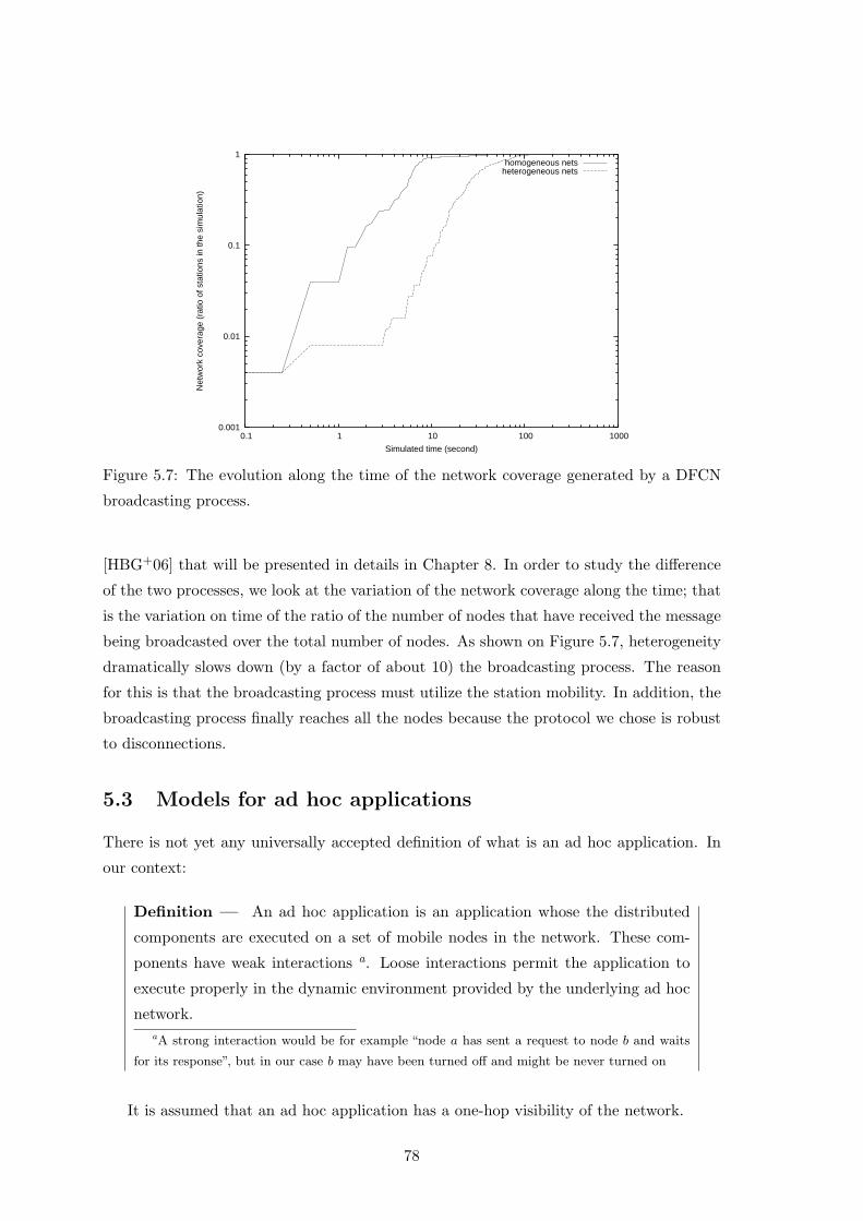
0.001
0.01
0.1
1
0.1 1 10 100 1000
Net
wor
k co
vera
ge (
ratio
of s
tatio
ns in
the
sim
ulat
ion)
Simulated time (second)
homogeneous netsheterogeneous nets
Figure 5.7: The evolution along the time of the network coverage generated by a DFCN
broadcasting process.
[HBG+06] that will be presented in details in Chapter 8. In order to study the difference
of the two processes, we look at the variation of the network coverage along the time; that
is the variation on time of the ratio of the number of nodes that have received the message
being broadcasted over the total number of nodes. As shown on Figure 5.7, heterogeneity
dramatically slows down (by a factor of about 10) the broadcasting process. The reason
for this is that the broadcasting process must utilize the station mobility. In addition, the
broadcasting process finally reaches all the nodes because the protocol we chose is robust
to disconnections.
5.3 Models for ad hoc applications
There is not yet any universally accepted definition of what is an ad hoc application. In
our context:
Definition — An ad hoc application is an application whose the distributed
components are executed on a set of mobile nodes in the network. These com-
ponents have weak interactions a. Loose interactions permit the application to
execute properly in the dynamic environment provided by the underlying ad hoc
network.aA strong interaction would be for example “node a has sent a request to node b and waits
for its response”, but in our case b may have been turned off and might be never turned on
It is assumed that an ad hoc application has a one-hop visibility of the network.
78

Examples of ad hoc applications have been given in Section 3.
Within Madhoc, an application can be executed on a subset of the nodes in the
network. Moreover, several applications can be executed on one single node.
5.3.1 Connections/disconnections
In order to enable the nodes to be aware of new neighbors, simulators sometimes use
event-driven notification. More precisely, when the simulator finds a new link, it dynami-
cally invokes a handler method on the two nodes involved. This method, defined abstract,
must be implemented by the application that defines what to do in case of a connec-
tion/disconnection event. This application of the observer design pattern, based on poly-
morphism, has proved elegant and flexible. However, Madhoc assumes that event-based
programming can hardly be used in the context of the simulation of ad hoc applications.
Instead Madhoc provides all nodes with an utility method that returns a set of the nodes
that were not yet in range last time it was invoked. Applications are then free to invoke
this method or not.
Note: Another drawback of the event-based notification is that the code of handler
methods is executed by the kernel of the simulator in a routine dedicated to the construc-
tion of the interconnection network: a routine that should not execute any application-level
code.
5.3.2 Application identification
As nodes can execute several applications, there is the need to have a way of identifying
the different applications running on one given node. Madhoc defines that applications
running on a given node are identified by their class (similarly, IP identifies processes by
their port numbers). Madhoc does not allow two applications with the same leaf class
to execute on one single node. Similarly, TCP/IP or UDP/IP do not allow two servers
processes to share the same port.
5.4 Simulation model
In this section is detailed the way the simulation engine is modelled. It focuses on the
components that participate to the particularities of Madhoc.
5.4.1 Time management
Time management is a critical issue to any simulation engine. This section details the way
Madhoc makes use of time and how it schedules the execution of the applications over
time.
79

5.4.1.1 Discrete-time simulation
Unlike many other simulators, Madhoc is not a discrete-event simulator. Instead of
jumping from event to event, the kernel of Madhoc iterates from time steps to time
steps. It hence discretizes time. The time-interval between two iterations is called the
resolution.
The resolution of a simulation process is defined by the user. The greatest is the
resolution, the faster—and the less accurate—is the simulation process. The resolution of
the simulation ideally depends on the application the user want to simulate. In the specific
case of RAD1-based broadcasting, the resolution should be at least twice smaller than the
maximum RAD otherwise the benefit of using a RAD is simply lost. In the specific case
of the simulation of mobility, the resolution should ensure that mobile nodes move with
reasonably low speed, otherwise some connections that would have occurred in the real
world would not be simulated.
5.4.1.2 Simulator internal scheduler
The application scheduler implemented in the core of the simulator works in a sequential
manner. The reason for this is performance: because Madhoc is not likely to run on
massively parallel computers, dedicating one thread by node would have been way too
cumbersome and the number of simulated nodes would have been a lot lessened.
Practically, the scheduler manages a list of the simulated applications. It iterates on
this list by giving to each application the opportunity to execute.
Initially the list of nodes on which the scheduler iterated always featured the same
order. On runtime, we could notice that some nodes processed faster that others, that some
nodes transmitted over the network without any problems while other nodes constantly
could not. We then noticed that on the low-bandwidth communication links, only a few
nodes were able to transmit before the link was saturated, the others—if any— were
blocked. Moreover these privileged few nodes were always the same, the scheduling was
hence unfair.
In order to give all applications the same chance to execute and to emit data on
the network during an iteration of the simulator, the application scheduler performs in a
stochastic fashion. More precisely, along one single iteration, all applications are asked to
execute multiples times, each time for a very short period. The order of the applications are
invoked is randomized. At each turn all applications are invoked, but in a non-predefined
order.
1Random Assessment Delay
80

5.4.2 Simulation area and network projections
Madhoc defines that the mobile nodes evolve in a square area. The surface of this area
can be defined by the user. The number of nodes in the simulation area does not vary
over time: the simulation area is assumed to be closed.
Instead of measuring the effects of its application on all nodes in the network, the user
might want to consider only a subset of it. For example, he may want to observe what
is going on only on a specific zone of the simulation area, he may want to observe what
happens only on Bluetooth nodes, etc. In order to make this possible, Madhoc defines
the concept of network projection. Just like the mathematical definition of projection,
Definition — A projection of the simulated network is a subset of the nodes
that match a given criterion. The network links retained in the projection are
the links whose the two nodes involved have been retained in the projection.
The metrics available in the simulation will be used on each projection, generating
several measure repositories. Several projections have been predefined.
Network
Projection
sourceNetwork projectionResult
MeasureHistory
measureMap0..n
Sensor
measureMap0..n
IdentityProjection NetworkInterfaceBasedProjection
RoundWindowProjection
WindowProjection
SquareWindowProjection
Figure 5.8: An UML representation of the concept of network projection.
As convenient as projections are, processing the projections is a cumbersome task for
the simulator: at each iteration it needs to find out which nodes belong to a projection,
and then apply the measurement available on this newly created set of nodes. It is then
important that the user defines only the projections that are relevant to him.
Madhoc has a set of predefined projections, among which:
identity projection gathers all the stations in the initial network. This is the most basic
projection as it projects everything.
81

window projection considers a sub-area of the simulation area whose center is the center
of the latter. The window can be either a square or a circle. The size of the window
is parametrizable.
network technology-based projection considers the subset of the nodes in the net-
work that embeds a network adapter of a given type.
only-connected-nodes projection gathers all the nodes that have at least one neigh-
bor.
random projection is a projection made of a set of nodes that are randomly selected.
This projection is useful if the user wants to operate on a subset of the simulated
nodes—for performance reasons, for example—while keeping a certain degree of sta-
tistical confidence.
5.4.3 Monitoring the ad hoc applications
A “monitor” aims at deploying, initializing and monitoring the ad hoc applications it is in
charge of. It is an abstraction defined at the level of the simulation. It does not have any
instance in the real world. It serves as the software interface between the user and a set
of applications running on the network nodes.
In particular, monitors provide the user with software sensors which allow him to ob-
serve what is going on in the simulation process. Just like a physical sensor (thermometer,
barometer, etc), a Madhoc sensor will take measures on a given system. Measures are
taken at each iteration. Each new measure is appended to an history.
Unfortunately, sensing takes time. The more sensors, the longer the simulation. Then,
for the development process, it is advisable to use as many sensors as possible in order to
detect the slightest flaw of the code, but for the research experimentation campaign, it is
better enabling only the metrics which will be used for result interpretation.
5.4.4 Termination of the simulation process
A simulation is said to be terminated if all the applications it executes are terminated.
Sometimes the mere concept of termination does not make sense to some application.
For example, the “beaconing” application (which consists in periodically emitting “hello”
packets in the neighborhood so that the node can build a 1-hop neighborhood information)
has no reason to terminate. In such a case, the application is not considered in the
termination condition of the simulation.
Since the termination condition of an application depends on it, it must be defined by
its developer.
82

5.4.5 Random number generation
Random number generation is an important feature of simulators. Madhoc uses one single
random number generator. This generator uses a gaussian law. This random number
generator can be seeded by:
• a fixed number, making all the runs be the same;
• the system clock, which has as a result that experiments started at different time
will execute in different manners. When seeding with the system clock, several
experiments executed at the same time on different nodes of a clusters in which
nodes are time-synchronized (NTP—Network Time Protocol) will be the same;
• the IP address of the computer running the simulation. This makes the simulta-
neous execution be different. By coupling a fixed number to the system clock, the
experiments become reproducible, which is a necessary condition for scientific exper-
imentation. ;
• a combination of the system clock and the local IP address, which makes all runs
differ, whatever host is used and whenever the simulation is executed.
83

Chapter 6
Modelling Mobility
The representation of mobility is a key issue in mobile networks simulation. The literature
mentions loads of mobility models which cover various aspect of human mobility. If it
were possible to combine them, the community would be provided with a fairly complete
representation of how people move. However in practise, only one of them is of common use:
the random waypoint mobility model. Researchers propose more and more sophisticated
mobility models, using for example real traces or realistic radio waves propagation models.
This chapter presents the contributions of this thesis in the topic of mobility for mobile
ad hoc network simulation. Primarily, Chapter 6.1 provides an overview of the mobility
models used in ad hoc network simulation, and presents a set of mobility models aiming
at simulating the motion of citizens. Chapter 6.2 it introduces a classification of mobility
models. Finally Section 6.4 is presented a new mobility model called the Human Mobility
Model.
6.1 State of the Art
Mobility models are considered as a major issue in the field of simulation of mobile ad
hoc networks. This section introduces the concept of mobility models, then it describes
two classifications of such models, prior to finally exposing the ones which are subject to
global agreement and usage.
6.1.1 Preliminary discussion
As explained in [TG05],
Definition — a mobility model is a set of rules used to generate trajectories
for mobile entities. Mobility models are used in network simulations to generate
network topology changes due to node movement.
84

This vision of a mobility model is very often broadened by some research groups which
associate the notion of movement to other notions like environmental properties or radio
propagation. For example, the UDEL mobility model [BS04b] defines that radio waves
bounce onto walls, using ray-tracing.
Mobility models aim at reproducing the reality of stations mobility. In the context
of city-based environments, researchers try to design environmental models of the cities
and to reuse human mobility patterns that define how people move in such environments,
some also develop radio propagation models that take into consideration the impact of
environmental components on the way radio waves get spread. Thus, mobility models
should be defined in such a way that they allow the simulation of real-world situations.
For instance, let us consider a limited number of lanes on roads, coupled with an important
flow of vehicles. This situation may lead to the apparition of traffic jam lines. If cars used
inter-vehicle communication systems, then the topology of the local network would globally
look like a chain. Simulators should be able to reproduce this kind of scenario since the
topology is of great importance in the achievement of most of mobile ad hoc networks
applications.
6.1.2 Mobility models in use
There exists a variety of mobility models which are currently used within the mobile ad hoc
networking community. The most popular one is the random waypoint mobility model. It
is described in Section 6.1.2.2. The most important mobility models are presented in the
following.
6.1.2.1 Random walk mobility
Random walk is extensively described in [PN04, Bet01]. It defines that a mobile node
moves from its current location to a new location by randomly choosing a direction and
speed in which to travel. The new speed and direction are both chosen from pre-defined
ranges, [speedmin; speedmax] and [0; 2π] respectively. Each move in the Random Walk
Mobility Model occurs in either a constant time interval t or a constant distance travelled
d. At the end of a move, a new direction and speed are calculated. If a node which moves
according to this model reaches a simulation boundary, it “bounces” off the simulation
border with an angle determined by the incoming direction.
There exists many variations of the random walk mobility model. For instance the
Random Direction Mobility Model forces nodes to travel to a boundary of the simulation
area before changing direction and speed.
85

6.1.2.2 Random waypoint mobility
Random waypoint is the most popular mobility model. In the random waypoint mobility
model, as described in [BRS03], each node randomly chooses a destination location (in
terms of its x, y coordinates) in the simulation area and moves towards this destination
with a randomly chosen velocity. When the destination is reached, the station remains at
the same place for a while. Once this time expires, the node chooses a random destination
in the simulation area and a speed that is uniformly distributed in [minspeed,maxspeed].
The node then travels toward the newly chosen destination at the selected speed. This
process is repeated by each station until the end of the simulation.
Often in the model, the nodes are initially distributed randomly around the simula-
tion area. As long as the simulation runs, the space distribution of the nodes tends to
some “stable value”, referred to as its “stationary distribution”. However this stationary
distribution does not exhibit a fair distribution of the nodes over the simulation area, and
might lead to some troubles when simulating. This problem is detailed by [NC04].
The random trip [BV05] mobility model is a generic mobility model that generalizes
random waypoint and random walk to realistic scenarios. It is implemented in ns-2. The
implementation performs perfect initialization meaning that the mobility model has no
transient phase.
6.1.2.3 Obstacle mobility model
The obstacle mobility model [JBRA+05, JBRAS03] is a realistic mobility model which
incorporates obstacles in the simulation area. These obstacles are utilized to both restrict
nodes movements as well as wireless transmissions. In addition to the inclusion of obstacles,
it constructs movement paths using the Voronoi diagram [Aur91] of obstacle vertices. More
precisely, the obstacle mobility models defines that the obstacles are polygons. Polygons
point are considered to be Voronoi points. This permits the calculation of the Voronoi
partition of the simulation space. Every Voronoi partition is defined by a set of segments.
Any segment which does not have any point within an obstacle is considered to be a
possible movement path. Nodes can then be randomly distributed across the paths, and
can use shortest path route computations to destinations at randomly chosen obstacles.
Simulation results shows that the use of obstacles and pathways has a significant impact on
the performance of ad hoc network protocols. The obstacle mobility model is implemented
in several simulators, including ns-2 and GloMoSim.
6.1.2.4 City-section mobility
The mobility of the vehicles in town gathers a lot of interest among the researchers as
well as among the businesses implicated in vehicular ad hoc networks. A variety of city
86

mobility models were defined. The two models described below belong to those.
6.1.2.4.1 City Section Mobility Model In the City Section Mobility Model, the
simulation area is a street network that represents a section of a city where the ad hoc
network exists. The streets and speed limits on the streets are based on the type of city
being simulated. For example, the streets may form a grid in the downtown area of the
city with a high-speed highway near the border of the simulation area to represent a loop
around the city. Each mobile node begins the simulation at a defined point on some
street. A mobile node then randomly chooses a destination, also represented by a point on
some street. The movement algorithm from the current destination to the new destination
locates a path corresponding to the shortest travel time between the two points. Upon
reaching the destination, the mobile node pauses for a specified time and then randomly
chooses another destination (i.e., a point on some street) and repeats the process.
6.1.2.4.2 Manhattan mobility model The Manhattan mobility model is proposed
to model movement in an urban area. In the Manhattan model, the mobile node is allowed
to move along the horizontal or vertical streets on the urban map. At an intersection of
a horizontal and a vertical street, the mobile node can turn left, right or go straight. The
probability of moving on the same street is 0.5, the probability of turning left is 0.25
and the probability of turning right is 0.25. Manhattan mobility model focuses on nodes
moving along horizontal or vertical streets, which is not enough to model nodes moving
along non-horizontal and non-vertical paths. Moreover, Manhattan model is not suitable
to model the movement happening in the intersections of highway systems, which is much
more complex than the intersection of local streets.
6.1.2.5 Group mobility models
In entity mobilities, the motion of the nodes does not depend on the motion of other
nodes. However, there are many situations where it is necessary to model the behavior of
mobile nodes as they move together. In order to model such situations, group mobility
models [HGPC99] are needed to simulate this cooperative characteristic. For example, a
complex specific mobility model was defined for the simulation of troop mobility [BZG04].
More generally, A variety of generic group mobility models were defined, as detailed in the
following.
6.1.2.5.1 Reference point group mobility The Reference Point Group Mobility
(RPGM) model represents the random motion of a group of mobile nodes as well as the
random motion of each individual mobile node within the group. Group movements are
based upon the path travelled by a logical center for the group. Individual mobile nodes
87

randomly move about their own pre-defined reference points, whose movements depend
on the group movement.
6.1.2.5.2 Columobile node mobility model The Columobile node Mobility Model
proves useful for scanning or searching purposes. This model represents a set of mobile
nodes that move around a given line (or columobile node), which is moving in a forward
direction. A slight modification of the Columobile node Mobility Model allows the indi-
vidual mobile nodes to follow one another. Each mobile node is placed in relation to its
reference point in the reference grid; the mobile node is then allowed to move randomly
around its reference point via an entity mobility model.
6.1.2.5.3 Nomadic community mobility model Nomadic Community Mobility
Model: a set of nodes move together from one location to another. Within each com-
munity or group of mobile nodes, individuals maintain their own personal spaces where
they move in random ways. In the Nomadic Community Mobility Model, each mobile node
uses an entity mobility model (e.g., the Random Walk Mobility Model) to roam around
a given reference point. When the reference point changes, all mobile nodes in the group
travel to the new area defined by the reference point and then begin roaming around the
new reference point. The parameters for the entity mobility model define how far a mobile
node may roam from the reference point. Compared to the Columobile node Mobility
Model, the mobile nodes in the Nomadic Community Mobility Model share a common
reference point versus an individual reference point in a columobile node.
6.1.2.5.4 Pursue Mobility Model Pursue Mobility Model: a set of nodes follow
a given target. As the name implies, the Pursue Mobility Model attempts to represent
mobile nodes tracking a particular target. The random vector value is obtained via an
entity mobility model. The amount of randomness for each mobile node is limited in order
to maintain effective tracking of the mobile node being pursued. The current position of
a mobile node, a random vector, and an acceleration function are combined to calculate
the next position of the mobile node.
6.1.2.6 Boundless Simulation Area
The mobility models described hereinbefore are considered to operate in a simulation area
that is geographically limited. The presence of bounds leads to topological specificities such
as a non-uniform distribution of the nodes in the simulation area. This also participates
to the appearance of dynamical phenomenons like nodes which get in contact too often
because they are in the same edge of the simulation area.
88

The Boundless Simulation Area Mobility Model is an attempt to limit these harmful
effect. It consists in converting a 2D rectangular simulation area into a torus-shaped one.
A node reaching an edge of the simulation areas, instead of bouncing onto the edge, will
show up at the opposite edge of the area.
However this technique has to be used with care because it also has harmful effects.
For instance, consider a broadcasting process which starts at one corner of the simulation
area. The broadcasted message is supposed to cross—by jumping from node to node—the
simulation area. But because of nodes instantly travelling to the opposite corner, the
message is able to cross the simulation area much faster than it would be able to do it in
reality.
6.1.3 Characterizing mobility models
From the user point of view, mobility models differ in the resulting network topology they
generate and the way this topology varies upon time. When it comes to mathematically
characterizing these mobility models, most researchers have recourse to the spatial distri-
bution of the nodes across the simulation area to the degree distribution of the network
graph.
6.1.3.1 Space/speed distribution
As detailed in [NC04], the distribution of the initial locations and speeds of the nodes dif-
fers from the distribution at later points in the simulation. Furthermore, the probability
distributions of both location and speed generally vary continuously over time and con-
verge to a “steady-state” distribution, known in the probability literature as the stationary
distribution.
6.1.3.2 Link duration
The link duration of a given network connection is the time elapsed between its establish-
ment and its break down. The average link duration is the average duration for all links
that appear along the simulation. This metric is important because bandwidth-demanding
protocols may not be able to operate at all with (too) short link durations.
Sometimes simulators consider that a link is available as soon as two nodes get in
range, that is the distance to each other is lower than a given threshold. In practise
this is not true. More precisely when the network adapter of a given node detects the
presence of an electro-magnetic signal, it first need to synchronize on it, in order to be
able to communicate with the other nodes sharing this same medium. This process can
take a while and its duration can never be neglected. For example, in the case of nodes
89

implementing the Bluetooth specification, it is commonly observed that two nodes in range
need a few seconds to be able to get synchronized, that is to communicate.
Considering that nodes may move fast, it is very probable that two nodes moving in
opposite direction cannot communicate with each other (even if they get very close to each
other at some moment) because the time for establishing the data connection is greater
than the time required for them to become out of range of each other.
6.1.3.3 Degree distribution
The number of nodes that are neighbors of a node n is called the degree of n. The degree
distribution D(k) gives the probability that a selected node has exactly k links. The degree
distribution provides useful information in the framework of the study of mobile ad hoc
networks. Particularly it clearly indicates wether the network is partitioned or not: in a
partitioned network, the probability of finding a node which has a zero degree is greater
than zero.
6.1.3.4 Neighbor density
The neighbor density of a given node is the number of nodes which are within radio range.
In networks in which the space distribution is homogeneous, the average neighbor density
is a relevant measure.
6.2 A new classification for mobility models
The aim of this section is to provide a comprehensive classification methodology that
considers every important behavioral and structural feature of mobility models. The clas-
sification presented hereinafter is based on seven criteria which are: whether or not the
mobility model considered makes use of randomness, whether or not it uses predefined
movement data, whether or not its motion is ruled by the motion of other nodes, whether
or not the way it moved in the past impact the way it will move in the future, whether or
not the environment in which it moves features some geographical constraints. The two
last criteria are whether all the nodes in the simulation obey the same mobility rules or
not, and if their motion is directed by the simulation application. All these characteristics
are summarized on Table 6.1 and detailed below.
6.2.1 Randomness
A mobility model is said to be randomized if it makes use of randomness. Generally
constant, the degree of randomness is sometimes adjustable, like in the groups mobility
models in which nodes follow a given direction with a certain degree of imprecision in the
90

name random trace group memory spat. const. plural app. driven
Random walk yes no no weak no no no no
Random Waypoint yes no no weak no no no no
Obstacle yes no no weak yes no no yes
Nomadic yes no yes weak no no no no
Pursue yes no yes weak no no no no
HMM yes no no strong yes yes no yes
City yes no no strong yes yes no yes
Table 6.1: A classification of the mobility models.
movement. Resorting to stochastic mobility is generally a good idea since it is the sole
way to achieve a high number of mobility configurations (or particular ones) with little
coding.
6.2.2 Traces
A mobility model is said to be using traces if it makes use of real data on the motion
of people. Trace information is now available thanks to some geographical studies which
aimed at defining the activity of the citizen during the day.
6.2.3 Group/entity
A mobility model is said to rely on “group” if the decision of how a given station moves
is based upon the motion of other stations. In opposition, “entity” mobility models define
nodes that move independently. Group mobility models can be sub-classified in terms of
locality/centrality according to the amount of station location information they require.
More precisely, a station uses a localized collaborative mobility model if its motion is
decided based on some mobility information (speed, angle, etc) of the stations around. On
the contrary, a mobility model that requires a global (or quasi-global) knowledge of the
motion of the stations in the network is said to be centralized.
6.2.4 Memoryful/less
A mobility model is said to be memoryful if the decision of how a given station moves is
based upon how the station moved in the past. There exists huge variation regarding the
amount of information memorized by mobile nodes during their travel. Generally only the
previous location (the location at the previous step of the simulation) is stored and reused.
Storing more information would be useful to generate more realistic motion on the long
run.
91

6.2.5 Spatial constraints
A mobility model is said to be spatially constrained if there exists a point in the simulation
area to which a station cannot be located.
A station moving according to the random waypoint mobility model could be located
at any point in the simulation area; thus the random waypoint mobility model is spatially
unconstrained. On the contrary, a station moving according to the obstacle mobility model
cannot be located within the bounds of an obstacle, consequently the obstacle mobility
model is spatially constrained.
6.2.6 Plurality
A mobility model is said to be plural if there exists at least two stations whose motion is
not directed by the same rules.
For instance, the mobility model defined in [BZG04] relies of distinct mobility rules to
ensure a certain heterogeneity on how devices move.
6.2.7 Application-driven
A mobility model is said to be application-driven if there exists a node which deliberately
moves in a way so that it helps an application to operate. Once again, in the specific case
of ad hoc network simulation, an application-driven mobility model can be classified either
as localized or centralized, depending upon the amount of information it requires to tune
its rules.
As an example of application-driven mobility, consider the mobility of the police in the
case it has to warn the population of some danger: the policemen cross the city in such a
way that they maximize the number of people who can hear the signal.
6.3 New metrics for mobility models
As described in Section 6.1.3 the network topology resulting from the application of mo-
bility models is commonly analyzed in terms of node speed, spatial distribution and degree
distribution. For some specific studies researchers resort to metrics such as the cluster-
ing coefficient, shortest path length, etc. In the context of the study of broadcasting
and topology control, better metrics for the structural analysis of ad hoc networks were
needed.
6.3.1 Size of the greatest connected component
When considering realistic communication technologies and mobility models, it appears
that networks may be largely partitioned. This is because of the limited radio range of the
92

nodes, their uneven spatial distribution and PHY-level synchronization issues. The size of
the partitions observed may vary greatly.
This metric is particularly useful in the context of research on topology control proto-
cols. More precisely, a topology control protocol primarily aims at improving the connec-
tivity of the network. Briefly this can be achieved by dynamically adjusting the power of
the antennas, on the basis of a variety of rules. Another solution is making clever use of
directional antennas. Sometimes different solutions are used: disconnected partitions can
become connected by the use of a backbone network such as GSM or UMTS. The chal-
lenge is then to find the network nodes which will take the initiative of connecting to the
backbone in such a way that both the number of partitions and the cost are minimized.
6.3.2 Probability of meeting again
When dealing with security issues, it is important to know how frequent is it to meet some
node that we have met in the past. This is especially important when working on trust
and reputations. In this context, the average time for two nodes in range to get in contact
again is clearly relevant.
6.4 Human mobility
Human mobility is the default mobility model in Madhoc. It is a generic mobility model
that roughly represents the intention-driven mobility of people in metropolitan areas.
Simulating metropolitan mobility is difficult because urban zones feature an extensive
list of dissimilar configurations (avenues, pedestrian areas, places, shopping malls, etc).
Building a generic model that takes into consideration all the components of a city is
a daunting task. So far, attempts at modelling metropolitan mobility focus on specific
configurations. The UDEL mobility model [BS04b] is one of the most advanced initiatives.
Humans do not move randomly. When moving, they have a determined target spot
and move towards it. The target may be a few meters away (next shop, next crossroads,
other sidewalk, etc) as well as far away (next district, next city, etc). Upon time, their
target changes. Most of the time, people have a dynamically changing list of targets. This
list of target spots is dynamically changing because of various parameters that will appear
upon time (locations of the target places, closure times, high frequentation times, etc).
6.4.1 Algorithm
The human mobility model defines that the simulation area is a bounded area. This area
contains a set S of destinations for nodes. These destinations are called “spots”. A spot is
located by its x, y coordinates. It is a round area defined by the length of its radius. Spots
93

do not overlap. Nodes can be located either in or out of spots. The mobility model used
by the node which move out of a spot is a variant of the random walk mobility model.
On the first hand, when a node n is located out of any spot, it must choose a destination
spot d(n). To do this, it maintains a set V S(n) of the spots it visited in the past. A node
cannot visit twice a same spot. d(n) is chosen so as it is the closest spot which has not
yet been visited (which does not belong to V S(n)). The node then move towards its
destination spot, with a certain degree of random variation in its direction. The direction
is periodically adjusted; this ensures that the node will eventually reach its destination
spot at one moment. The mobility of nodes out of any spot is a specialization of the
random walk mobility.
On the other hand, when the node n is within a spot d(n), it moves according to the
random direction mobility models. When the node reaches the edge of the spot, d(n)
is added to V S(n) and a new destination spot d(n) must be defined. If all spots have
been visited (V = V S(n)) then V S(n) is emptied and the search for a new destination is
triggered again.
6.4.2 Radio waves
The human mobility model (HMM), just like the obstacle and UDEL mobility models,
defines that the elements which constraint the motion of the node also rule the propagation
of the radio waves. It assumes that spots are surrounded by a circular wall, and that walls
have an absorbtion ratio ranging from 0 to 1. 0 means that the wall does not impact the
radio signal. 1 means that the signal is totally blocked. An intermediate value means that
the signal is proportionally attenuated. HMM does not model how the signal bounces.
6.4.3 Scenarios
6.4.3.1 Mall
The mall scenario represents people wandering within a shopping mall. The spots stand
for shops. They are located randomly with a constraint for non-overlapping. The mall
scenario can generate highly dense wide areas. It allows to study the behavior of protocols
in dense network conditions.
6.4.3.2 City-center
The city-center environment represents people walking and driving in the streets of a
city center. The spots stand for crossroads. They are located according to a grid-like
structure. Their location is then slightly randomly modified using an amplitude specified
by the researcher. Nodes move faster outside of the spots than inside. The city-center
94
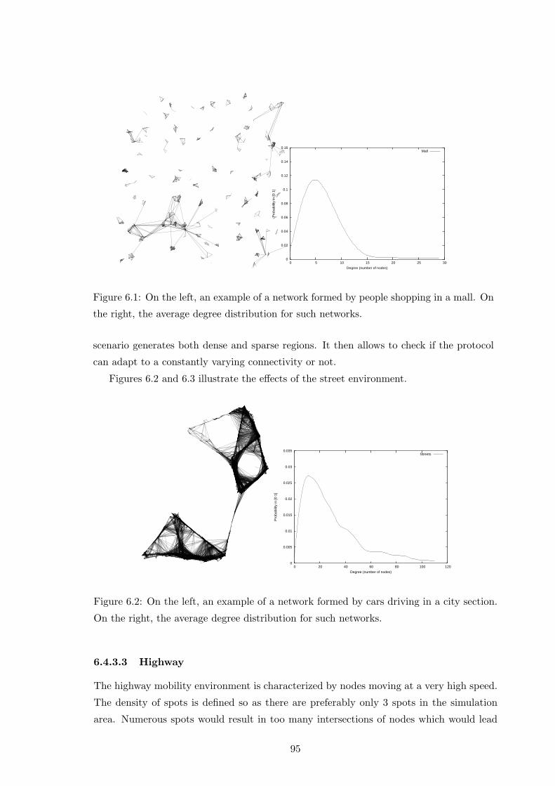
0
0.02
0.04
0.06
0.08
0.1
0.12
0.14
0.16
0 5 10 15 20 25 30
Pro
babi
lity
in [0
1]
Degree (number of nodes)
Mall
Figure 6.1: On the left, an example of a network formed by people shopping in a mall. On
the right, the average degree distribution for such networks.
scenario generates both dense and sparse regions. It then allows to check if the protocol
can adapt to a constantly varying connectivity or not.
Figures 6.2 and 6.3 illustrate the effects of the street environment.
0
0.005
0.01
0.015
0.02
0.025
0.03
0.035
0 20 40 60 80 100 120
Pro
babi
lity
in [0
1]
Degree (number of nodes)
Streets
Figure 6.2: On the left, an example of a network formed by cars driving in a city section.
On the right, the average degree distribution for such networks.
6.4.3.3 Highway
The highway mobility environment is characterized by nodes moving at a very high speed.
The density of spots is defined so as there are preferably only 3 spots in the simulation
area. Numerous spots would result in too many intersections of nodes which would lead
95

Figure 6.3: The graph resulting of the simulation of 2,000 nodes roaming in a 1km2 area.
Nodes have a either IEEE802.11b or a Bluetooth interface, with the same probability.
to unrealistic behavior. The highway environment is very different from the other ones in
the sense that the connectivity it produces is specific: most links are organized into chains
of nodes moving in opposite senses.
As the nodes move very fast, the duration of connections is very short. The highway
scenario then allows to check if an application is opportunistic enough.
Figures 6.4 and 6.5 illustrate the effect of the highway environment.
6.4.4 Open issues
6.4.4.1 Initialization of the mobility
As long as the simulation runs, the space distribution of the nodes converges to a stable
state known as the stationary distribution. Except in some specific cases (for example if
the mobility model is analytic) the stationary distribution is not known at the moment
the simulation starts. An issue is hence where to locate the nodes at the beginning of the
simulation. Until the stationary distribution is reached, the results of the simulation cannot
be considered valid. A solution would then be to wait for this stationary distribution to
be reached. Unfortunately in the case of the human mobility model, if the evolution of
the space distribution is clearly visible on 2D graphs, we did not figure out which metric
should be used to automatically detect it. Even if we experimentally found out some
rules of thumbs making it possible to detect the stationary distribution in many cases, the
strategy did not prove versatile enough to be applied on the variety of configurations of
the human mobility model.
96

0
0.02
0.04
0.06
0.08
0.1
0.12
0.14
0.16
0.18
0.2
0 2 4 6 8 10 12 14 16 18
Pro
babi
lity
in [0
1]
Degree (number of nodes)
Highway
Figure 6.4: On the left, an example of a network formed by cars driving on a highway
section. On the right, the average degree distribution for such networks.
6.4.4.2 Defining the resolution of the simulation
The concept of resolution is described in Section 5.4.1.1. The resolution of the simulation is
definable by the user. The lower the resolution step, the more precise the simulation. If the
user needs to simulate bigger networks or longer periods of network activity, increasing
the resolution may be necessary, otherwise the simulation would be too slow. But the
higher the resolution step, the less precise the simulation. There is no theoretical upper
limit for the resolution step. The question is: what is the threshold of the resolution step
above which the simulation process does not output precise-enough results? Madhoc
has initially been developed considering a fixed resolution of four iterations per second,
with was a reasonably precise time step in the context of the simulation of broadcasting
protocols for mobile ad hoc networks. In the later versions of Madhoc, the resolution
of the simulation has become a user-definable parameter. On the one hand, applications
such as clock synchronization [CW04] require much more precise simulations. On the other
hand, applications like the dissemination of trust information [SKJ+00] does not have to
deal with short communication delay and hence can be simulated using greater resolution
steps.
97

Figure 6.5: The interconnection graph resulting of the simulation of 100 nodes driving on
a 3 kilometers-long highway section. Most of the nodes have a Bluetooth adapter as well
as a IEEE802.11 one.
98

Part III
Broadcasting across mobile ad hoc
networks
99

Broadcasting—also called flooding—is one of the earliest research interests about mo-
bile ad hoc networking. This is because broadcasting constitutes one of the fundamental
low-level network operations which serves as the basis of higher level applications such as
routing. Traditionally, broadcasting means sending a message from one given node (the
source station) to all the nodes in the network. In a (multi-hop) decentralized network,
the broadcasted data has to be relayed by intermediate nodes in such a way that all the
network graph is spanned. However in mobile ad hoc networks, broadcasting cannot be
defined in these terms. Indeed the limited radio range of the nodes and their mobility
make that all the nodes might not be reachable all the time. As a consequence, the mere
definition of broadcasting had to be adapted: the broadcasting problem across mobile ad
hoc networks can be seen as a multi-objective problem targeting at maximizing the num-
ber of nodes reached, at minimizing the time required to reach them, and at minimizing
the network overhead. This latter objective is particularly important because too much
emissions (causing great network overhead) may lead to the congestion of the network;
this problem is known as the broadcast storm problem.
In networks with no or slow mobility, spanning trees-based methods prove effective.
Briefly they aim at determining the minimal set of relay nodes that must participate in
the broadcast process. In networks whose nodes have high velocity, different strategies are
employed. These strategies are all based on local neighborhood information. They include
Probabilistic schemes, Scalable Broadcasting Algorithm (SBA), Multipoint Relaying, Ad
hoc Broadcasting Procotol (AHBP), etc. While these strategies operate well when the
network density is such that the network is connected, they fail as soon as some partitions
appear. An extension of AHBP (called AHBP-EX) overcomes this problem by triggering
re-emission on the discovery of a new neighbor. This strategy unfortunately generates
too high network overhead. Additionally, SBA and AHBP, which are the most effective
protocols in their class, assume 2-hop neighborhood information. In reality, when the
mobility is high, it is still not sure that 2-hop information is achievable.
The broadcasting protocols which have been targeted at mobile ad hoc networks are
presented in Section 7. Then Section 8 introduces Delayed Flooding with Cumulative
Neighborhood (DFCN), a protocol which exhibits better results in terms of the network
overhead it generates as well as in terms of broader range of mobility models and node
density it tolerates.
100

Chapter 7
State of the Art
Network broadcasting commonly consists in sending a packet from one node to every node
in a network. When considering fixed network, the main issue of broadcasting is to find
the spanning tree [PR02] of the network; that is the subset of the network nodes that span
all the nodes. The Spanning Tree Protocol, which is also referred to as STP, is defined in
the IEEE Standard 802.1d, and later, in 1998, the Rapid Spanning Tree Protocol (RSTP)
(defined by the 802.1w specification) operates very well in the context of fixed networks.
When dealing with mobile networking, and particularly with mobile ad hoc networking,
the protocols described hereinbefore are not applicable.
The main challenge when broadcasting across mobile ad hoc networks comes from its
inherent mobility. Because in such network the network links are volatile, the Spanning
Tree Protocol cannot be applied as is. There exists strategies, based on dynamic spanning
trees, which consist in maintaining an accurate spanning tree as long as the nodes move
[SW04]. The nodes are likely to move fast, consequently the technique for updating the
spanning tree must be extremely reactive. In this context, [Cas06] have developed a
method which ensures that the maintenance of the spanning tree after a node move is
achieved in one single operation. Their algorithm, which is a localized one (it runs on
every devices, relying on 1 or 2 hops neighborhood information, see section 7.3.3), is well
suited to large mobile ad hoc networks, in which localized protocols are preferred. However,
these techniques make the implicit assumptions that the mobility (if some) is low and that
the network is non-partitioned (meaning that all nodes are reachable through multi-hop
connections). Some other protocols [RP04], proposed more recently, feature more dynamic
approaches (such as self-pruning [WC02]), in which the mobility is central issue. The
protocol presented inhere belongs to the latter category. More precisely, its aim is to enable
efficient broadcasting in networks in which the topology is very heterogeneous and dynamic.
This is the case of the metropolitan ad hoc networks (MobileMANs). MobileMANs are
described in Section 1.1.5. In such network, the broadcasting process cannot propagate
data to all nodes: only a subset of the nodes can be reached at a given time.
101

7.1 Technical challenges
This section lightens some of the main issues that must be faced during the design of
broadcasting protocols.
7.1.1 Hidden and exposed node problems
The hidden node problem (defined in Section 5.2.2.1) constitutes a major obstacle to
broadcasting. More precisely, this issue makes it impossible to ensure that, within a
given network partition of the network, all nodes will be reached. This problem could be
overcome by the use of acknowledgement packets (ACKs) but doing this would be contrary
to the very principle of broadcasting which is to minimize the number of packet emission.
Consequently, the actual target of broadcasting within mobile ad hoc network is to reach
as many nodes as possible, ideally all of them.
Without the use of acknowledgement packets, even a broadcasting protocol which
theoretically ensures that all nodes will be reached would turn out to fail at reaching a
subset of them.
7.1.2 Mobility and Partitioning
The mobility of the nodes constitutes another major challenge broadcast protocols have
to deal with.
On the one hand, mobility constitutes an obstacle to the operation of the broadcast
protocols based on spanning trees. Thanks to algorithms like [Cas06], it is now possible to
deal with dynamic spanning trees in efficient and distributed ways. However these tech-
niques operate regardless of the application they serve. In the specific case of broadcasting,
the spanning tree should be constructed on the basis of the (continuously growing) set of
nodes that have received the message. Since localized protocols have no kind of global
information on the network, doing so is challenging.
On the other hand, mobility (when applied in realistic networking parameters) in-
evitably leads to partitioned networks. Network partitioning constitutes one of the great-
est issues when it comes to broadcasting. In particular, broadcasting protocol must find
a technique which allows the broadcast message to “jump” from partition to partition,
in order to reach as many nodes as possible. This idea is central to epidemic diffusion
models.
7.2 Protocols
This section described the broadcasting protocols that are seen as referenced in the liter-
ature and commonly used for experiments.
102

Most often broadcasting protocols make use of a random assessment delay (RAD).
When a given node a receives a broadcast message from another node b, if it decides to
forward it, this does not happen immediately. Instead it will wait a certain duration picked
randomly in [0, max delay] ms. This delay is called the random assessment delay (RAD)
before re-emitting. When b sent the message, its others neighbors, if any, also received
the message at the very same time as a. So if all neighbors which decide to forward the
message do it immediately, collisions are highly likely to happen. Randomly delaying every
emission dramatically reduces the risk of collisions.
7.2.1 Simple Flooding
As explained in [WC02], in the Simple Flooding [OVT01] each node forwards received
messages exactly once. Simple Flooding does not make any attempt to reduce the num-
ber of re-broadcasting nodes and does not require any knowledge. This strategy is not
suitable for environments with high density regions because it would then generate too
much network traffic and sometimes could even lead to network congestion. This problem
is referred to as the broadcast storm problem [NTCS99].
7.2.2 Probabilistic scheme
Upon the reception of a broadcast message, a node executing a probabilistic broadcasting
protocol will forward the message with a probability p and will take no action at all
regarding this message with a probability 1− p. Then the value of p depends on the user
of the protocol. If p = 1 then the probabilistic scheme behaves just like simple flooding.
The value of p should be adapted according to the topological properties of the network
the protocol will be executed on.
7.2.3 Distance-based methods
In distance-based methods, the decision of forwarding broadcast messages depends on the
estimation of the distance between nodes. The distance between nodes can be estimated
according to the electrical strength of the received radio signal. A node a receiving a
broadcast message from another node b will compute the distance d between a and b. If
d is lower than a given threshold t, then the message is dropped because a assumes that
the (short) extra distance that would be covered by a new emission would not justify the
expense (in terms of bandwidth and battery consumption) of one emission.
7.2.4 Area-based methods
Area-based methods are very similar to distance-based methods, which are presented in
Section 7.2.3. In area-based schemes, nodes do not evaluate the benefit of a new emission
103

in terms of the extra distance that would be then covered. Instead they base their decision
on the basis of the extra surface that would be covered. If the devices are equipped with
omnidirectional antennas, surfaces are calculated using the strong assumption that the
coverage area of nodes is circular, which is wrong most of the time.
7.2.5 Flooding with Self-Pruning
Flooding With Self-Pruning (FWSP) [WC02] which implements a neighborhood-aware
strategy based on 1-hop knowledge. Each broadcast message includes the list of identifiers
of the neighbors of the sender node. FWSP-enabled nodes upon reception of a broadcasted
message retrieve the set of identifiers embedded in the message and subtracts it to the set
of identifiers of its own neighbors. If the resulting set is empty, the message is dropped,
otherwise it is forwarded.
7.2.6 Scalable Broadcast Algorithm
SBA [PL00] implements a neighborhood-aware strategy based on 2-hops knowledge. SBA
differs from Flooding with Self-Pruning only in the neighbor-knowledge it requires. Each
SBA broadcast message includes a list of identifiers of the 2-hop neighbors of the sender
node. The strategy carried out by SBA-enabled nodes is as following: upon reception of a
broadcasted message, the node retrieves the set of identifiers embedded in the message and
subtracts it to the set of identifiers of its own neighbors. If the resulting set is empty, the
message is dropped, otherwise it is forwarded. SBA also defines a technique which consists
in re-adjusting the RAD (see section 7.2) according to the degree of the node concerned
and the maximum degree of its neighbors.
7.2.7 Multipoint relaying
Just like SBA, Multipoint Relaying [LQV01] relies on the knowledge of 2-hops neighbor-
hood. Multipoint Relaying’s messages contain the set of nodes that must act as relays.
Multipoint Relaying then works this way: upon message reception, the node finds out if
its identifier is contained in the message-embedded set of relays. If yes, it constructs the
smallest set of 1-hop relays that cover all the 2-hop neighbors. In turn, it embeds this set
in the broadcast message itself before sending it around. The construction of the set of
the forwarding nodes is done according to the greedy algorithm described in [Lov75].
7.2.8 Ad Hoc Broadcast Protocol (AHBP)
The Ad Hoc Broadcast Protocol (AHBP) [PL01] AHBP is based on the Multipoint Re-
laying protocol. In AHBP, only nodes who are designated as a Broadcast Relay Gateway
(BRG) within a broadcast packet header are allowed to rebroadcast the packet. BRGs are
104

proactively chosen from each upstream sender which is a BRG itself. The algorithm for a
BRG to choose its BRG set is identical to the one used in Multipoint Relaying.
The main difference between AHBP and Multipoint Relaying is that a node using
AHBP informs 1-hop neighbors of the BRG designation within the header of each broadcast
packet. This allows a node to calculate the most effective BRG set at the time a broadcast
packet is transmitted. In contrast, Multipoint Relaying informs 1-hop neighbors of the
MPR designation via “hello” packets.
7.2.9 AHBP-EX
AHBP-EX [PL01] is an extension of the AHBP 7.2.8 protocol. It aims at supporting
high mobility networks. Its strategy is as follows: upon detection of a new neighbor, the
node re-trigger the AHBP strategy consisting of designing 1-hops neighbors as relays and
emits the message. Upon experiments, this technique proved to generate a huge network
overhead. In some cases in which the node density is high and nodes move fast, it even
generates more network overhead than simple flooding does.
7.2.10 INOP
INOP [CSP06] is designed to use two-hop neighborhood information. It utilizes a novel
technique for determining the transmission power level at each node during the broadcast.
Each transmitting node first sorts its neighbors based on the required power to reach them.
Then, starting from the closest neighbor, the node compares the required power levels to
reach the next neighbor either directly or indirectly via some other neighbor. Based on
this comparison, the transmitting node decides on the transmission power level to use in
its broadcast.
Simulation based comparisons the existing set of variable power approaches (BIP
[WNE00], PABLO, (AHBP) have shown that compared to other variable power approaches,
INOP achieves better results in terms of energy efficiency, and competes and exceeds other
approaches in terms of a number of other performance metrics including traffic overhead,
coverage, and convergence time.
7.3 Classifications
There exists three classifications for the mobility models, as detailed in the following.
7.3.1 Camp’s classification
Williams and Camp [WC02] classify broadcasting protocols according to the network
knowledge that the nodes need to have in order to execute them. They define four cat-
105

egories: simple flooding, probability-based methods, area-based methods and neighbor-
knowledge-based methods. This categorization is based on the way protocols select re-
broadcasting nodes.
In Simple Flooding [NTCS99], nodes forward received broadcast messages exactly once,
which could lead to network congestion.
In probability-based methods [NTCS99], nodes forward received broadcast messages
with a certain probability. This probability is locally re-evaluated every time a message
is received. Probabilistic scheme, just like simple flooding, require not information on the
network.
When information about nodes location is available, the decision of re-broadcasting
a given packet can be taken according to the additional geographical area covered by a
potential emission. Area-based and location-based [NTCS99] methods define that if the
surface or distance of this area is lower than a given threshold, the message is not re-
emitted. Network information can be obtained by GPS or evaluated by triangulation or
by measuring the power of the radio signals.
Finally, neighbor-knowledge-based methods (SBA, Flooding With Self-Pruning (FSWP),
AHBP, Multi-point Relaying, etc) require the knowledge of some neighborhood informa-
tion (FWSP uses 1-hop neighbors, SBA, Multipoint Relaying and AHBP uses 2-hops
neighbors). They constitute the last class of broadcasting strategies. This class can be
divided in two subclasses: neighbor-designating and self-pruning methods. On the one
hand, the nodes running protocols belonging to the neighbor-designating subclass (AHBP,
Multipoint Relaying) operate by designing their neighbors that will be in charge of relaying
the message. On the other hand, the nodes running protocols belonging to the self-pruning
subclass (SBA, FWSP) decide by themselves whether to rebroadcast or not.
7.3.2 Stojmenovic’s classification
Stojmenovic and Wu [SW04] recently proposed some classifications for broadcasting pro-
tocols. In their proposal protocols can be classified according to their algorithmic nature
(determinism, reliability) or the information required by their execution (network infor-
mation, “hello” messages content, broadcast messages content).
A broadcasting algorithm is said to be deterministic if it behaves predictably. If it
runs on a particular input, it will always produce the same output. Most broadcasting
protocols are deterministic.
An algorithm is assumed to be reliable if it ensures that all nodes in the network will
be covered. Probabilistic schemes and area-based methods (see section 7.2) are usually
unreliable as they rely on randomness and heuristics, respectively. Note that the concept
of reliability does not make sense if the network is partitioned. In such case reaching all
the nodes is not possible to achieve.
106

Protocol Scope Deter. Reliable Mobility
DFCN 1-hop yes no yes
Simple flooding - yes yes no
Location-based 1-hop yes no no
Probabilistic - no no no
FWSP 1-hop yes yes no
SBA 2-hop yes yes no
Multi-point relaying 2-hop yes yes no
AHBP-EX 2-hop yes yes yes
Figure 7.1: The table summarizes the properties of the broadcasting protocols mentioned in
the paper. It provides, correspondingly, the name of the protocol, the amount of topology
information it requires, whether it uses a deterministic approach or not, whether its is
reliable or not, and if it takes into consideration the mobility of nodes.
7.3.3 Wu’s classification
Another classification was proposed by Wu and Lou [WL03]. It is based upon the amount
of state information required for performing broadcasting. More precisely, they categorized
protocols on whether they rely on a global, quasi-global, local or quasi-local knowledge of
the network. Global and quasi-global broadcasting algorithms are also called centralized
protocols. Centralized protocols are listed in [Pel02]. Their main drawback is that they
are not scalable. They are hence unusable in the MANETs. Localized protocols are those
which need a local (or quasi-local) view of the network. Example of the protocols belonging
to this class are 1 and 2-hops neighborhood-knowledge protocols.
The network state information (node’s identifier, location, degree), and network topol-
ogy information are interchanged between nodes. Such information is carried by either
“hello”messages (which are specifically meant to represent topology information) or broad-
cast messages. The amount of data embedded in those messages has a serious impact on
the network throughput. Protocols can then be classified according to the amount of data
is carried either in the “hello” or broadcast messages [SW04].
107

Chapter 8
DFCN
In this section we present the Delayed Flooding With Cumulative Neighborhood (DFCN)
protocol. DFCN related papers are [HGB04, HBG+06, LND+06].
First the objectives for the DFCN protocol are given in Section 8.1. Then its strategy
is detailed in Section 8.3. Further, the iterative (and chronological) construction of DFCN
is given in Section 8.3.2. Then the effectiveness of DFCN is illustrated in detail through
experiments, in Section 8.4. Finally, Section 9 describes the application of some multi-
objective optimizations of DFCN, aiming at tuning it at best.
Using Stojmenovic and Wu’s classification (see sections 7.3.2 and 7.3.3), DFCN is a
deterministic algorithm. It does not consist in a new approach for calculating dominating
sets. Instead it defines heuristics based on local network information. Only 1-hop infor-
mation is required, which permits DFCN to achieve very good level of scalability. The
“hello” messages exchanged by the nodes do not carry any additional information. Only
broadcast messages must embed the list of node neighbors.
Using Williams and Camp’s classification (see section 7.3.1), DFCN belongs to the
self-pruning neighbor-knowledge-based class.
8.1 Objectives
The objectives of the Delayed Flooding with Cumulative Neighborhood (DFCN) are man-
ifold:
1. to provide a protocol which has lower network overhead. Scalable Broadcast Algo-
rithms (SBA), the Ad Hoc Broadcast Protocol (AHBP), and Multipoint Relaying
are some of the most efficient in terms of network overhead.
2. to provide a protocol which operates well regardless of the network density. More
precisely, as illustrated on Figures 8.1 and 8.2, broadcasting in a low density network
(top-left figure, 50nodes/km2) is difficult because the protocol needs to make a very
108

good use of the mobility to achieve a good coverage. When the density increase
(top-left figure, 1, 000 nodes/km2), the connectivity gets better, but the network
may be partitioned. When the network is highly connected (bottom left and right
figures, respectively 5, 000 and 10, 000 node/km2), the broadcasting protocol must
be bandwidth-efficient in order to minimize the risk of packet collisions.
3. to provide a localized protocol which operates with 1-hop neighborhood information.
Both SBA and AHBP require 2-hops neighborhood information. One challenge is
then to achieve better performance by using less network information.
Figure 8.1: The node density in a network impacts greatly its topology. Broadcasting
protocols should be able to operate regardless of the density condition. Up to now, few
protocols support such great variation of the node density.
Not knowing the network size in advance makes the goal of reaching all nodes impossible
to measure in practice. Furthermore, minimizing the duration of the broadcasting process
109

0.0001
0.001
0.01
0.1
1
1 10 100
Pro
babi
lity
in [0
1]
Degree (number of nodes)
50010005000
10.000
Figure 8.2: The evolution of the average degree distribution when the density grows
is not always the primary target.
8.2 Requirements
For being able to run the DFCN protocol, the 4 following assumptions must be met:
1. Like many other localized neighbor-knowledge-based broadcasting protocols (FWSP,
SBA, etc) and as mentioned in the previous section, DFCN requires the knowledge
of 1-hop neighborhood. One way of obtaining this information is by using “hello”
packets. We denote the set of neighbors of the node s by N(s).
2. Each message m embeds in its header the set of IDs of the 1-hop neighbors of its
most recent sender. We refer to this set as T (m).
3. Each node maintains local information about all messages received. Each instance
of such information consists of three items:
• the ID of the message received;
• the set of IDs of the nodes that are known to have received the message, referred
to as K(m);
• the decision of whether the message should be forwarded or not, referred to as
a(m).
110

4. DFCN requires the use of a RAD before possibly re-emitting a broadcast message
m. The random delay for a given message m is referred to as r(m).
8.3 DFCN’s strategy
In this section, the DFCN protocol is presented. The strategy for decision making relies
on a set of reactive and proactive rules, implemented in components that are described
and explained in the next sections. Before entering the details, let us perform a careful
analysis of the problem. Broadcasting in mobile ad hoc networks in the context of DTNs
corresponds to the search of a trade-off that can be expressed as meeting two criteria:
reaching as many stations as possible (first criterion), and limiting the number of ree-
missions (second criterion). In order to reach as many stations as possible, the protocol
executed on each node should decide of a reemission as soon as new stations are encoun-
tered. If such a strategy is applied when the network is sparse, this would lead to good
results for both criteria since every reemission prove to be useful because of the reduced
number of meeting points between station. And thanks to the low density of the network,
the number of reemission should be limited. However the same strategy applied in a dense
environment would lead to catastrophic results in terms of useless (re)-emissions. Indeed,
in a dense network, the number of events corresponding to the meeting of two stations that
don’t know each other is a huge number. Unfortunately, in the context of metropolitan
environments, both situations may occur. Some areas may be underpopulated while other
may be, at the same time, densely populated. As a consequence, the decision part of the
protocol should rely on the perceived density of the station, which density corresponds
directly to its neighborhood. We achieve this adaptivity with the help of two thresholds:
minBenefit and densityThreshold. The first, minBenefit, measures the oppotunity to (re)-
emit a message according to the composition of the neighborhood. This threshold is built
as the ratio between the number of new stations in the neighborhood, over the total num-
ber of stations in the same neighborhood. When a suitable ratio of new stations appear in
the neighborhood, the node (re)-emit the message. But, when the density is too low, this
only mechanism leads to poor performances. To prevent this problem, the other threshold,
densityThreshold was defined in order to allow the release of the limitation of the previous
mechanism. The next section describes in details how these thresholds are embeded in the
different components that compose DFCN.
8.3.1 Description of the algorithm
When a node receives a message, the forward decision may depend on different elements:
RAD, neighborhood, density, etc. In order to allow the protocol to self-adapt to the
customer application but also to the density, we have introduced a new parameter called
111

”benefit” that will be further described.
As previously mentioned in the ”DFCN requirements” (section 8.2, first item), a node s
maintains for a message m a list K(m) which contains the identifiers of the nodes that are
known to have already received m. The list K(m) is managed as follows: when s sends a
message m to its neighbors, it knows that all of them will receive m (unless some collisions
occur). If ever the same situation happened (if s had the same neighborhood), then m
would not be forwarded again, as all the nodes around are already known to have received
it. When a node n receives a message m from one of its neighbors b, it also adds all the
neighbors of b in K(m), as all of them should have received m as well.
However, this simple mechanism is too reactive. Indeed, as soon as a new station
becomes present in the neighborhood, the message is re-emitted. And in some situations,
especially when the density is very high, this may entail a continuous re-emission of the
messages. In order to prevent such scenario, we use the minBenefit threshold which is
formally defined as the ratio between the number of neighbors of s which do not belong to
K(m), and the number of neighbors of s: |N(s)−K(m)||N(s)| . The smaller is the required benefit,
the less DFCN will be restricted in emitting messages, hence the lower throughput it will
generate.
The behavior of DFCN is driven by three events. These events are:
• the reception of a message referred to as reactive behavior
• the expiration of the RAD of some messages
• the detection of a new neighbor referred to as proactive behavior.
When one of these three events occurs, DFCN reacts by behaving in a specific manner,
as described in the following sections.
8.3.1.1 Message reception event
If a message m is received for the first time, K(m) is equal to T (m) and a RAD is then
assigned to m. Otherwise the set T (m) and the ID of the sender node are added to K(m).
This behavior corresponds to algorithm 1.
Figure 8.3 gives an example of this behavior. Here the threshold densityThreshold is
set to 0.2. The node s holds a message that is candidate to broadcast. The black node is a
new neighbor of s. Since s knows that only 2 neighbors out of 12, (ratio of 2/12 = 0.16) do
not hold the message, s does not emit the message. On the right figure, 6 of them do not
have the message yet, the ratio is then 6/12 = 0.5 which is greater than densityThreshold.
The message is then emitted.
112

Algorithm 1: The section of the algorithm executed upon message reception.Data: m: the incoming broadcast message
Data: s: the node which has sent m
if m is received for the first time then1
K(m)← T (m)2
rad(m)← random ∈ [0,maxRAD]3
else4
K(m)← K(m) ∪ T (m) ∪ s5
end6
K
K
K
K
K
K
K
K
SK
KK
K
K
K
S
Ratio = 2/12 = 0.16 < 0.2
No forward
Ratio = 6/12 = 0.5 > 0.2
Forward
Figure 8.3: An example of the DFCN reaction to the reception of a new message.
8.3.1.2 RAD expiration event
When the RAD of a message expires, its hosting node computes the ratio of neighbors that
did not yet receive it. If the ratio is greater than the threshold minBenefit, the message
is forwarded, otherwise it is dropped. If the message is emitted, then N(s) is added to
K(m). Algorithm 2 expresses this behavior.
8.3.1.3 New neighbor event
Each time a node s gets a new neighbor, the RAD for all messages is set to zero. Mes-
sages are hence immediately candidate to emission. If N(s) is less than the threshold
densityThreshold, this behavior is disabled. Algorithm 3 expresses this behavior.
Figure 8.4 gives an example of this behavior. Here the threshold densityThreshold is
set to 0.45. The node in the center holds a message that is candidate to broadcast. The
black node is a new neighbor of the center node. Since the center node has more than
10× densityThreshold neighbors it does not emit the message.
113

Algorithm 2: the decision function defines if a given message is worthwhile to be
forwarded or not.Data: the broadcast message m, candidate to immediate emission.
Data: s: the node that receives m
benefit← |N(s)−K(m)||N(s)|1
a(m)← benefit ≥ minBenefit2
if a(m) then3
K(m)← K(m) ∪N(s)4
end5
Algorithm 3: The algorithm executed upon message reception. M(s) is the set of
messages received—and not yet expired—by the node s.Data: s: the node which has a new neighbor.
if |N(s)| < densityThreshold then1
foreach m ∈M(s) do2
rad(m)← 03
end4
end5
8.3.2 Reactivity and Proactivity in DFCN
This section presents the reactive and proactive aspects of the DFCN protocol and the
way they impact its performances. It also discusses the way both approaches were coupled
in order to improve the results with respect to the aforementioned criteria: minimizing
the network traffic while maximizing the number of reached stations. In order to illustrate
this analysis, some intermediate results are presented. These results were obtained by
varying the density in [0, 10.000] nodes by square kilometer. Since the simulation area
was 250, 000m2 (500 × 500m), the number of nodes varied from 0 to 2,500. Finally, in
order to achieve some decent statistical confidence, the various measures were obtained by
averaging the measures out of 30 distinct simulations.
8.3.2.1 Reactive behavior
The reactive part of the DFCN protocol can faithfully be compared to all reactive-only
protocols (like Simple Flooding, SBA, AHBP, etc). Experiments (Figure 8.6) show that all
the reactive-only protocols tested here exhibit a linear increase of the number of emissions
with respect to the number of nodes, and thus they are linearly dependent of the density
value.
114

6 neighborsNo reemission
4 neighborsReemission
Figure 8.4: An example of the DFCN reaction to a new neighbor event.
Intuitively, if the number of rebroadcasting nodes was lessened proportionally to the
density increase, the average number of emissions should be bounded. DFCN relies on
this intuition. Practically, the threshold minBenefit which depends on the size of the
neighborhood is intended to play a major part for that. Experiments confirm that this
threshold has a serious impact on the performance of DFCN. By testing several values in
its definition interval ]0, 1[ (see Figure 8.5), we found out that the number of emissions
performed by DFCN increases as the threshold grows, the best value being 0.5. When using
values greater than 0.55, DFCN does not work at all. Because the performance drop-off
is sharp, one can consider that using 0.5 is risky. Then for the experiments presented
hereinafter, we used 0.4, which is considered safer. 0.4 is a safer because because 0.5 is
the upper limit for the ”controllable” behavior of DFCN. When using 0.6, DFCN did not
work properly. Using 0.5 solved the problem. Since we could not find out with precision
the “limit” value, we consider 0.5 to be the actual limit. A value below the limit had to be
chosen. The value 0.4 is then arbitrary.
The results presented on Figure 8.6 show that using DFCN, the number of emissions
in the network remains low as the density in the network grows. Moreover, it appears that
AHBP/SBA carry out at least 2.5 more emissions than DFCN.
8.3.2.2 Proactive behavior
Reactive strategies do not operate if the density of the network is lower than a given
threshold densityThreshold. The reason is that below this threshold, the network is
split in several partitions, preventing the broadcasting message to propagate. A common
solution to this issue is to re-execute the broadcasting strategy each time a new neigh-
bor connects. This technique is used—and proved effective—by the AHBP-EX protocol.
DFCN uses it too. This behavior is here referred to as proactive. As illustrated by Fig-
115

0
5
10
15
20
25
30
35
0 0.2 0.4 0.6 0.8 1
Num
ber
of e
mis
sion
s
Threshold (minBenefit)
Threshold
Figure 8.5: The number of emissions obtained when applying various values for the
minBenefit thresholds when the density is 2,000.
ure 8.7, this technique permits to DFCN (as well as AHBP-EX) to operate with success
when the density is as low as 100 devices per square kilometer.
Moreover, because the proactive strategy of DFCN uses the same decision function as
the one used by the proactive strategy, DFCN behave smoother: unlike AHBP, DFCN
does not systematically emit broadcast messages. The impact of this feature is clearly
visible on Figure 8.7, DFCN emits about twice less than AHBP-EX.
8.3.2.3 Reactive and proactive coupled
Even though the proactive strategy is efficient, it leads to poor performances when the
density is higher than 1,000. By probing the behavior of the reactive and proactive parts
of both AHBP-EX and DFCN, we found that the pro-action spoils the qualities of the
reactive behavior (see Figure 8.8). More precisely, when the density increases, the number
of proactive message emissions is way too high. The reason is simple: as the density
increases, there are more connections/disconnections, hence more message emissions. But
most of these proactive emissions are actually totally useless.
DFCN solves this problem by using the threshold densityThreshold defined in Sec-
tion 8.3.2.1. More precisely, DFCN disables its proactive strategy when the number of
neighbors is greater than densityThreshold (see Figure 8.9). This turnaround makes
both the reactive and proactive strategies to operate only when they are needed (see Fig-
ure 8.10). densityThreshold = 4 has experimentally shown to be a good value. Figure
8.11 shows that using the threshold improves the performance of DFCN, by dramatically
reducing the number of messages emitted by the proactive strategy. As a matter of fact,
116

0
100
200
300
400
500
600
700
0 1000 2000 3000 4000 5000 6000 7000 8000 9000 10000
avg_
num
ber_
of_e
mis
sion
s
Network density (station/km^2)
FloodingWithSelfPruningMultipointRelaying
PurelyReactiveDFCNSBA
SimpleFlooding
Figure 8.6: The reactive behavior of the DFCN protocol keeps the number of emissions
low, whatever the network density is.
when the density is high—more than 2, 500node/km2—the proactive strategy does not
operate anymore.
8.3.2.4 Application domain
As explained in Section 8.1, the network density has a serious impact on the behavior of
broadcast protocols. Experiments show that, given any broadcast protocol, there exists
a density threshold below which that protocol does not work. the protocols that do
not feature any proactive management of the mobility (Simple flooding, SBA, Multipoint
Relaying, etc) are unusable in the environment where the density is lower than 1,000 nodes
by square kilometer.
Based on reaction to neighborhood changes AHBP-EX and DFCN perform well down
to 100 nodes/km2. Broadcasting in partitioned ad hoc networks relies on the mobility
of the nodes. Because there are several partitions in the network, the only way for the
broadcast message to jump from one partition to another is to find temporary paths
heading to other partitions or to be carried by nodes moving to other partitions. This
process may last a while, since the temporary paths appear erratically and the speed of
the nodes is limited.
8.4 Experiments
This section described the experiments which were conducted in order to show the prop-
erties of the DFCN protocol. The conditions of the experimentation are described, then
117
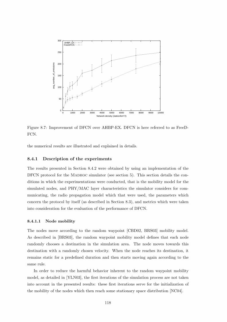
0
50
100
150
200
250
300
0 1000 2000 3000 4000 5000 6000 7000 8000 9000 10000
avg_
num
ber_
of_e
mis
sion
s
Network density (station/km^2)
AHBP_EXFreeDFCN
Figure 8.7: Improvement of DFCN over AHBP-EX. DFCN is here referred to as FreeD-
FCN.
the numerical results are illustrated and explained in details.
8.4.1 Description of the experiments
The results presented in Section 8.4.2 were obtained by using an implementation of the
DFCN protocol for the Madhoc simulator (see section 5). This section details the con-
ditions in which the experimentations were conducted, that is the mobility model for the
simulated nodes, and PHY/MAC layer characteristics the simulator considers for com-
municating, the radio propagation model which that were used, the parameters which
concern the protocol by itself (as described in Section 8.3), and metrics which were taken
into consideration for the evaluation of the performance of DFCN.
8.4.1.1 Node mobility
The nodes move according to the random waypoint [CBD02, BRS03] mobility model.
As described in [BRS03], the random waypoint mobility model defines that each node
randomly chooses a destination in the simulation area. The node moves towards this
destination with a randomly chosen velocity. When the node reaches its destination, it
remains static for a predefined duration and then starts moving again according to the
same rule.
In order to reduce the harmful behavior inherent to the random waypoint mobility
model, as detailed in [YLN03], the first iterations of the simulation process are not taken
into account in the presented results: these first iterations serve for the initialization of
the mobility of the nodes which then reach some stationary space distribution [NC04].
118

0
20
40
60
80
100
120
140
160
180
200
0 1000 2000 3000 4000 5000 6000 7000 8000 9000 10000
Avg
_num
ber_
of_e
mis
sion
s
Network density (station/km^2)
ReactivityProactivity
Figure 8.8: When the density is high, the proactive strategy of DFCN emits lots of mes-
sages. But with such density, the reactive behavior only would be sufficient for broadcast-
ing. The bandwidth utilization of the proactive behavior is then useless.
The simulated area is a square whose edge is 500m. The velocity of nodes is randomly
chosen between 3 and 6km/h. The pause lasts 5 seconds.
8.4.1.2 PHY/MAC
The coverage radius (maximum distance from the source from which the signal can be
sensed and demodulated) used for the simulations, can vary between 30 and 60 meters.
The maximum bandwidth (theoretically obtained when the signal is not attenuated and
when the link is free of interferences) is 11Mbps. These characteristics correspond to the
IEEE 802.11b specifications.
Communications are established according to the rules defined by the CSMA (Carrier
Sense Multiple Access) MAC layer. No collision management mechanism like CA (Collision
Avoidance) or CD (Collision Detection) is used here. CSMA was chosen because it is the
smallest common set of the specific MAC layers used by existing wireless networking
technologies (IEEE 802.11a/b/g).
8.4.1.3 Radio wave propagation
Radio wave propagation depends on the natural environment of the nodes. In open space
the propagation is omni-directional and the covered area is a circle. Some works aiming at
modelling the propagation of radio waves use techniques like advanced statistical models or
ray-tracing [BS04a]. For simplicity most of the works in the area of broadcasting considers
119

0
2
4
6
8
10
12
14
16
18
20
0 1000 2000 3000 4000 5000 6000 7000 8000 9000 10000
Avg
_num
ber_
of_e
mis
sion
s
Network density (station/km^2)
densityThreshold useddensityThreshold unused
Figure 8.9: The use of densityTheshold allows DFCN’s proactive strategy to become
discrete as the density increases.
the open space path loss as the radio wave propagation model. According to open space
path loss model radio signal gets attenuated as the distance grows.
8.4.1.4 Parameters of the protocol
As explained in Section 8.3.1, DFCN relies on the minBenefit and densityThreshold thresh-
olds. It has experimentally been found out that 0.4 and 4, respectively, are good values
for these threshold. The following benchmarks rely on these values.
8.4.1.5 Benchmarking process
The simulation of a broadcasting process starts with the selection of some random nodes.
These nodes are the starting places of the broadcast message. In order to prevent the
broadcasting process from starting from an isolated node (from which reactive-only pro-
tocols would have no chance to operate), the source node is chosen so that its number of
neighbors is greater than the average number of neighbors in the whole network.
The broadcasting process is said to be:
completed if it could satisfy the coverage constraint. Coverage satisfaction ensures the
validity of the broadcasting process. More presicely, if the coverage cannot reach the
constrained value, then the broadcasting process is considered to have failed.
failed if the broadcast message expires before the broadcasting process could satisfy the
coverage constraint. The lifetime of broadcasting messages depends upon the appli-
cation. Packet routing layers need quite short lifetimes while high-level applications,
120

0
50
100
150
200
250
300
350
400
0 1000 2000 3000 4000 5000 6000 7000 8000 9000 10000
Avg
_num
ber_
of_e
mis
sion
s
Network density (station/km^2)
ReactivityProactivity
Figure 8.10: The use of a threshold makes both the reactive and proactive strategies to
operate only when they are needed.
like advertising application, may want the message to be alive several hours. In our
simulations we set the message lifetime to 1 minute. Upon expiration of its life-
time the message can no longer be transmitted. Thus the broadcasting process is
terminated.
In order to evaluate the performance of the DFCN protocol, it is compared to other
competing protocols. As mentioned in Section 7.2, numerous broadcasting protocols have
been proposed. But not all of them have the same objectives as DFCN. More precisely, cen-
tralized (global and quasi-global) broadcasting protocols cannot be applied in the context
of mobile ad hoc networks. Protocols relying on location information like [SS00, NTCS99]
cannot be used as references because we assumed that such information is not available.
Similarly, some broadcasting protocols use mechanisms that enable the nodes to adjust
power of the transmitter and receiver of its communication interface [CSS02a]. As the
availability of such mechanisms is not assumed, DFCN is not compared to such protocols.
As a consequence, the retained protocols for the evaluation are Simple Flooding (sec-
tion 7.2.1), Flooding with Self-Pruning (section 7.2.5), the Scalable Broadcast Algorithm
(section 7.2.6), Multipoint Relaying (section 7.2.7), and AHBP-EX (section 7.2.9).
8.4.2 Results
Based on the simulation parameters described in Section 8.4.1, we illustrate and explain
the performance of DFCN.
121

0
50
100
150
200
250
300
0 1000 2000 3000 4000 5000 6000 7000 8000 9000 10000
avg_
num
ber_
of_e
mis
sion
s
Network density (station/km^2)
AHBP_EXDFCN
FreeDFCN
Figure 8.11: Improvement of DFCN over FreeDFCN and AHBP-EX. FreeDFCN stands
for “DFCN without densityThreshold”.
8.4.2.1 Number of emissions
The number of emissions is one of the most relevant measure because it has a direct impact
on the network bandwidth used (network overhead). This value has to be minimized.
Figure 8.12 shows the average number of emissions in case when only one node initiates the
broadcasting process. A situation when 10% of the nodes initiate broadcast simultaneously
is shown on Figure 8.13. In both cases it can be seen that DFCN emits far less messages
than Multipoint Relaying, one of the most bandwidth efficient protocol.
8.4.2.2 Number of redundant receptions
The number of redundant receptions directly depicts the waste of resources (bandwidth,
energy, etc). It has to be minimized. Figure 8.14 shows that DFCN uses about 3 times
less resources than its competing protocols.
8.4.2.3 Duration of the broadcasting process
We look here at the time required to complete the broadcasting process.
Figure 8.15 shows that DFCN is not the fastest broadcasting protocol. This result
comes from its selective strategy. Because DFCN carries out less emissions, the broadcast-
ing process needs more time to complete. It is a tradeoff (enlightened in several studies
on broadcasting protocols for ad hoc networks): the more greedy a broadcasting protocol
is, the faster it is.
122

0
100
200
300
400
500
600
700
0 1000 2000 3000 4000 5000 6000 7000 8000 9000 10000
avg_
num
ber_
of_e
mis
sion
s
Network density (station/km^2)
AHBP_EXDFCN
FloodingWithSelfPruningMultipointRelaying
SBASimpleFlooding
Figure 8.12: The number of emissions carried out by each broadcasting protocol. Only
one single node initiates a broadcasting process
8.4.2.4 Emission efficiency
Defining the quality of a protocol is application-dependent. The objective function may
rely on various parameters: speed, bandwidth consumption, bandwidth waste, etc. In our
work, we consider as a relevant measure of efficiency, number of emissionsnumber of nodes reached . The good
results shown by Figure 8.16 testifies that DFCN carries out message emissions when it is
really worthwhile.
8.4.2.5 Application to different topologies
DFCN was tested on a variety of network topologies. In particular its application in
the context of the random waypoint mobility model is described in the previous sections.
DFCN was also analyzed in the context of metropolitan mobility model, and in particular
on network generated by the use of the human mobility model (see section 6.4) and its
mall scenario (see section 6.4.3.1), which exhibits a greatly varying neighbor density. In
order to harden the conditions for broadcasting, different networking technologies were
simulated, that is a number of nodes had only a IEEE802.11b adapter, others had only a
Bluetooth adapter and some others had both.
The results observed were qualitatively very similar to those exposed hereinbefore.
It can hence be concluded than DFCN is robust, and it does not suffer from changing
conditions.
123

0
100
200
300
400
500
600
700
800
900
1000
0 200 400 600 800 1000 1200 1400 1600 1800 2000
avg_
num
ber_
of_e
mis
sion
s
Network density (station/km^2)
AHBPAHBP_EX
DFCNSimpleFlooding
Figure 8.13: The number of emissions carried out when 10% of the nodes initiate a broad-
casting process. Because of the computational limitations of the worknodes used for the
simulation, we could not use densities greater than 2, 000nodes/km2.
0
5000
10000
15000
20000
25000
30000
35000
40000
0 1000 2000 3000 4000 5000 6000 7000 8000 9000 10000
avg_
num
ber_
of_r
edun
dant
_rec
eptio
ns
Network density (station/km^2)
AHBP_EXDFCN
FloodingWithSelfPruningMultipointRelaying
SBASimpleFlooding
Figure 8.14: The number of redundant receptions generated by each broadcasting protocol.
124

0
5
10
15
20
25
0 1000 2000 3000 4000 5000 6000 7000 8000 9000 10000
sim
ulat
ed_t
ime
Network density (station/km^2)
AHBP_EXDFCN
FloodingWithSelfPruningMultipointRelaying
SBASimpleFlooding
Figure 8.15: The execution time of each tested broadcasting protocol. The lower the
better.
0
2
4
6
8
10
12
14
16
18
20
0 1000 2000 3000 4000 5000 6000 7000 8000 9000 10000
avg_
emis
sion
_effi
cien
cy
Network density (station/km^2)
AHBP_EXDFCN
FloodingWithSelfPruningMultipointRelaying
SBASimpleFlooding
Figure 8.16: The results testify that DFCN carries out message emissions when it is really
worthwhile.
125

Chapter 9
Optimization of the broadcasting
process
The Madhoc implementation of DFCN was used as the basis for a study of the multi-
objective optimization of broadcasting protocols, as described in the following.
This section first gives a basic overview of genetic optimization, then of multi-objective
optimization. Then it describes the DFCNT and the cDFCN problems. For both of them
it presents the adopted solution and the obtained results.
This research was conducted in tight collaboration with the team of Prof. Enrique
Alba (Malaga University).
9.1 Genetic optimization
As explained in [Nas], genetic optimization works on a population of individuals represent-
ing possible solutions to a specific problem. Each individual is evaluated using a fitness
value which is a measure of how well this individual is adapted to its environment. Indi-
viduals (which are represented by a genotype—a suitable sequence of bits) reproduction
rate is proportional to their fitness. The bit-coded representation of individuals creates a
quantization of the solution space. A genetic algorithm starts with an initial population
of candidate solutions or individuals, and modifies it until the population converges to
a solution. A problem-dependent fitness function must be chosen to measure the appro-
priateness of an individual. The modification of the population is achieved by using the
application of three genetic operators which are: selection, crossover, and mutation.
9.2 Multi-objective optimization
Contrary to single objective optimization (which can be achieved by using genetic algo-
rithms, as explained in Section 9.1), multi-objective optimization is not restricted to find
126

a unique solution of a given multi-objective problem, but a set of solutions known as
the Pareto optimal set. For instance, taking as an example the problem we are dealing
with, one solution can represent the best result concern the number of reached stations,
while another solution could be the best one concerning the makespan. These solutions
are said non-dominated, that is there do not exist any other solution that consists in a
Pareto-improvement of these. A pareto improvement is a solution that can make at least
one individual better, without making any other individual worse. The result provided
by a multi-objective optimization algorithm is then a set of non-dominated solutions (the
Pareto optima) which are collectively known as the Pareto front when plotted in the ob-
jective space. The mission of the decision maker is to choose the most adequate solution
from the Pareto front.
A general multi-objective optimization problem can be formally defined as follows:
Definition — Find a vector ~x∗ = [x∗1, x∗2, . . . , x
∗n] which satisfies the m inequal-
ity constraints gi (~x) ≥ 0, i = 1, 2, . . . ,m, the p equality constraints hi (~x) = 0, i =
1, 2, . . . , p, and minimizes the vector function ~f (~x) = [f1(~x), f2(~x), . . . , fk(~x)]T ,
where ~x = [x1, x2, . . . , xn]T is the vector of decision variables. ¥
The set of all values satisfying the constraints defines the feasible region Ω and any
point ~x ∈ Ω is a feasible solution. As mentioned before, we seek for the Pareto optimum.
Its formal definition is given by:
Definition — A point ~x∗ ∈ Ω is Pareto Optimal if for every ~x ∈ Ω and
I = 1, 2, . . . , k either, ∀i∈I (fi (~x) = fi(~x∗)) or, there is at least one i ∈ I such
that fi (~x) > fi (~x∗). ¥
This definition states that ~x∗ is Pareto optimal if there exists no feasible vector ~x
which would decrease some criterion without causing a simultaneous increase in at least
one other criterion. Taking as an example the problem we are dealing with, one solution
can represent the best result concerning the number of reached stations, while another
solution could be the best concerning the makespan.
The mission of the decision maker is to choose the most adequate solution of the given
multi-objective optimization problem from the resulting Pareto front.
9.3 The DFCNT problem
From the description of the previous section, the following DFCN parameters are to be
tuned:
127

minBenefit is the minimum benefit for rebroadcasting. This is the most important pa-
rameter for tuning DFCN, since minimizing the bandwidth should be highly depen-
dent on the network density. It ranges from 0.0 to 1.0.
lowerBoundRAD, upperBoundRAD defines the RAD value (random delay for rebroad-
casting in milliseconds). Both parameters take values in the interval [0.0, 10.0] mil-
liseconds.
proD is the maximal density (proD ∈ [0, 100]) for which it is still needed to use the
proactive behavior (i.e., reacting on new neighbors) for complementing the reactive
behavior.
safeDensity defines a maximum safe density of the threshold which ranges from 0 to 100
devices.
These parameters, i.e., a DFCN configuration, characterize the search space. Here,
the objectives to be optimized are: minimizing the makespan (in seconds), maximizing
the network coverage (percentage of devices having received the broadcasting message),
and minimizing the bandwidth used (in number of transmissions). Thus, we have defined
a triple objective multi-objective problem, which has been called DFCNT (standing for
DFCN Tuning). For obtaining the values of these objective functions we have used Mad-
hoc because it implements the DFCN broadcasting protocol. Our goal is to obtain the
Pareto front of DFCNT (and the corresponding DFCN configurations) in terms of these
three objectives.
9.3.1 Using a cellular genetic algorithm
Cellular genetic algorithms are a subclass of GAs in which the population is structured
in a specified topology, so that individuals may only interact with their neighbors. These
overlapped small neighborhoods help in exploring the search space because the induced
slow diffusion of solutions through the population provides a kind of exploration, while
exploitation takes place inside each neighborhood by genetic operations. In cMOGA,
the cGA that is considered herein, the population is structured in a 2D toroidal grid,
and the neighborhood defined on it always contains 5 individuals: the considered one
(position(x,y)) plus the North, East, West, and South individuals.
9.3.1.1 Targeted network
Three very different realistic scenarios, implemented in Madhoc, are used in this study.
These scenarios correspond to real world environments, and they aim at modelling a shop-
ping mall (see Section 6.4.3.1), a metropolitan area (see Section 6.4.3.2), and a highway
(see Section 6.4.3.3). They are detailed in the following:
128

DFCNT.Mall is a shopping center of 200×200 square meters of surface with densities of
800 stores and 2 000 devices per square kilometer. Stores are circles of radius between
1 and 10 meters, and the obstruction of the walls is computed with a penalty of 70%
in the signal strength. Finally, devices travel with a speed ranging between 0.3 and
1 m/s in the corridors and between 0.3 and 0.8 m/s when they are inside the stores.
The resulting network is illustrated on Figure 9.1.
DFCNT.Metropolitan . This environment has a surface of 400×400 square meters,
with a density of 50 spots (standing for crossroads) per square kilometer having a
circle surface of radius between 3 and 15 meters. The wall obstruction is in this
case higher than for the mall environment (up to 90%), and the density of devices
is 500 elements per square kilometer. When setting the speed of devices, the cases
when people move on foot or by car must be taken into account, so its value ranges
between 0.3 and 10 m/s when they are in a crossroad, and between 1 and 25 m/s in
other case (streets). The resulting network is illustrated on Figure 9.1.
Mall Metropolitan Area Highway
Figure 9.1: The three studied scenarios for mobile ad hoc networks.
DFCNT.Highway Madhoc for modelling the network with the particularity of setting
the wall obstruction to 0%. The simulated surface was set to 1000×1000 square
meters with a density of only 50 devices per square kilometer. These devices travel
at random speeds between 30 and 50 m/s. We define the roads as straight lines
connecting two spots, and we establish a density of only 3 spots (highway entrances
and/or exits) for modelling the scenario. The speed of devices within the spots
must be reduced to between 20 and 30 m/s. The size of each spot (length of the
entrance/exit) is set to a random value between 50 and 200 meters (spots radius
∈ [25, 100] meters). The resulting network is illustrated on Figure 9.1.
In order to make our studies more realistic, an observation window has been included
in the simulations, such that only the devices located in this window are taken into account
129

Table 9.1: Main features of the proposed environmentsMall Metropolitan Highway
Surface 40 000 m2 160 000 m2 1 000 000 m2
Density of spots 800 (shops/km2) 50 (crossroads/km2) 3 (joints/km2)
Devices
Speed out of spots 0.3–1 m/s 1–25 m/s 30–50 m/s
Speed in spots 0.3–0.8 m/s 0.3–10 m/s 20–30 m/s
Density 2 000 dev./km2 500 dev./km2 50 dev./km2
Wall obstruction 70% 90% 0%
for measurements. This makes it possible to simulate nodes exiting and joining the network
by entering or leaving the observation window, respectively. Therefore, the existence of
a changing number of devices in the network is allowed, as it is the case in real mobile
ad hoc networks. In all our tests in this work, this observation window covers 70% of the
whole area. As an example, Figure 9.2 shows that a mobile ad hoc network simulating a
mall environment (left), and the observation window that is studied (right); (70% of the
whole network). The circles represent the shops, while the points stand for devices (those
outside the observation window are grey colored, meaning that they are not considered for
measurements).
Observation window
Inside
Outside
Figure 9.2: The effects of introducing an observation window on the studied mobile ad
hoc network.
9.3.1.2 Experiments
cMOGA has been implemented in Java and tested on a PC with a 2.8 GHz Pentium IV
processor with 512 MB of RAM memory, and running SuSE Linux 8.1 (kernel 2.4.19-
4GB). The Java version used is 1.5.0 05. All the values presented are the average over 30
independent runs of cMOGA.
130

1
2
3
4
5
6
7
8
0
5
10
15
20
25
30
0.4
0.5
0.6
0.7
0.8
0.9
Coverage
Bandwidth
Mall
Coverage
Bandwidth
Metropolitan Area
05
101520253035
0
20
40
60
80
100
120
00.1
0.20.3
0.40.5
0.60.7
0.80.9
1
CoverageBandwidth
Highway
05
10152025
0
20
40
60
80
100
120
00.1
0.20.3
0.40.5
0.60.7
0.80.9
1
Duration
Duration Duration
Figure 9.3: Pareto fronts for the solution of the DFCNT problem over three environments
131

The Pareto fronts on Fig. 9.3 expose the design objectives of the DFCN protocol:
most of the plots (in the center of the clouds) provide sets of parameters that make
DFCN achieving a coverage rate close to 100%, keeping the network throughput very low.
What makes the DFCNT problem particularly interesting from an applicative point of
view is that it permits the decision maker to discard this default behavior by setting a
degree of coverage for the broadcasting application. Indeed not all applications require
the maximization of the coverage rate. For example, local advertising—which consists in
spreading advertisement messages to devices a few hops away from the source—needs the
broadcasting process to cease after a while. Sometimes high coverage is even to be avoided.
For example trying to achieve a high coverage on metropolitan mobile ad hoc networks
(which may realistically be made of thousands of devices) is harmful, since it is likely to
lead to severe network congestions.
9.3.2 Using scatter search
This section first briefly describes multi-objective scatter search algorithms, then it details
which parameters the experiments were conducted. Finally it presents the metrics that
were used in order to evaluate the significance of the results obtained, explains the result
themselves.
9.3.2.1 Multi-objective Scatter Search
This section presents the description of scatter search algorithms, then it gives an overview
of the Archive-based Scatter Search (AbSS) which is used here.
9.3.2.1.1 Scatter Search Scatter search [Glo97, GLM00, GLM03] has been success-
fully applied to a wide variety of optimization problems [GLM00], but it has not been ex-
tended to deal with multi-objective optimization problems until recently [NLD+05, Bea05,
dSCF04, NLA05]. This meta-heuristic consists of five methods: diversification generation,
improvement, reference set update, subset generation, and solution combination.
The scatter search technique starts by creating an initial set of diverse individuals
in the initialization phase. This phase consists in iteratively generating new solutions by
invoking the diversification generation method; each solution is passed to the improvement
method, which usually applies a local search procedure in an iterative manner, and the
resulting individual is included into the initial set P. After the initial phase, the scatter
search main loop starts.
The main loop begins building the reference set from the initial set by invoking the
reference set update method. The reference set is a collection of both high quality solutions
and diverse solutions that are used for generating new individuals. Solutions in this set
are systematically grouped into subsets of two or more individuals by means of the subset
132

Observation Window
Inside
Outside
(a) (b)
Figure 9.4: (a) MobileMAN, and (b) the effect of the observation window
generation method. In the next step, solutions in each subset are combined to create a new
individual, according to the solution combination method. Then, the improvement method
is applied to every new individual. The final step consists of deciding whether the resulting
solution is inserted into the reference set or not. This loop is executed until a termination
condition is met (for example, a given number of iterations has been performed, or the
subset generation method does not produce new subsets).
9.3.2.1.2 AbSS AbSS (Archive-based Scatter Search) [NLD+05] is based on the afore-
mentioned scatter search template (see section 9.3.2.1.1) and its application to solve
bounded continuous single objective optimization problems [GLM03]. It uses an external
archive for storing non-dominated solutions and combines ideas of three state-of-the-art
evolutionary algorithms for solving MOPs. In concrete, the archive management follows
the scheme of PAES [KC99], but using the crowding distance of NSGA-II [DPAM02] as a
niching measure instead of the PAES adaptive grid; additionally, the density estimation
found in SPEA2 [ZLT01] is adopted for selecting the solutions from the initial set that will
build the reference set.
9.3.2.2 Targeted network
In order to make the simulations more realistic , Madhoc has been extended with an
observation window such that only the devices located inside this window are taken into
account for measurements. This allow the number of devices in the network to change,
just like it happens in real mobile ad hoc networks. This feature of Madhoc is illustrated
on Figure 9.4, where both an example of a MobileMAN (a) and the effects of introducing
an observation window on it (b) are shown. In all the tests, this observation window is
70% of the total simulation area. The main parameters of Madhoc used for defining the
network characteristics are the following:
133

size: defines the network simulation area in terms of square meters.
density : is the average density of nodes per square kilometer (i.e., the number of devices
per square kilometer).
environment: determines the mobility model (see section 6.1) of the stations as well as
the radio wave propagation model (see section 6.4.2). That is, this feature defines
how the stations are moving as well as the area within which they are moving (open
areas, buildings, streets, etc.), thus determining how radio waves propagate.
9.3.2.3 Results
This section is devoted to present the experiments performed for this work. First we
describe the metrics used for measuring the performance of the resulting Pareto fronts.
Next, the parameterization of AbSS and Madhoc is detailed. Finally, the results of
DFCNT are shown and compared against cMOGA [ADL+05] (see section 9.3.1).
9.3.2.3.1 Metrics Three metrics for assessing the performance of both AbSS and
cMOGA were used: the number of Pareto optima that the optimizers are able to find,
the Set Coverage [Zit99] which allows two algorithms to be compared in terms of Pareto
dominance, and the Hypervolume [ZT98] which measures both convergence and diversity
at the same time in the resulting Pareto fronts. They are defined as:
Number of Pareto optima , which can be considered as a measure of the ability of the
algorithm for exploring difficult search spaces defined by hard MOPs like DFCNT.
Set Coverage , which is the set coverage metric C(A, B) calculates the proportion of
solutions in B which are dominated by solutions of A. A metric value C(A,B) = 1
means that all members of B are dominated by A, whereas C(A,B) = 0 means that
no member of B is dominated by A. This way, the larger the C(A,B), the better the
Pareto front A with respect to B.
Hypervolume which calculates the volume (in the objective space) covered by the non-
dominated solutions. Algorithms with larger hypervolumes are desirable.
9.3.2.3.2 Parametrization The behavior of Madhoc has been defined based on
three parameters: the size of the simulation area, the density of mobile stations, and
the type of environment. For our experiments, we have used a simulation area of 40,000
square meters, a density of 2,000 stations per square kilometer, and, from the available
environments of Madhoc, the mall environment has been used. This environment is in-
tended to model a commercial shopping center. People go from one store to another by
134

AbSS cMOGA
Metric average std average std t-test
Number of Pareto Optima 98.7586 2.8119 98.1053 2.9000 –
Set Coverage 0.9865 0.0103 0.9793 0.0076 +
Hypervolume 0.8989 0.0695 0.8199 0.0854 +
Table 9.2: Performance metrics for AbSS and cMOGA when solving DFCNT
these corridors, occasionally stopping for looking at some shopwindows. Both the mobility
of devices and their signal propagation are restricted due to the walls of the building. A
metropolitan mobile ad hoc network with such a configuration has been shown in Fig-
ure 9.4. The result shown were averaged out out five non-deterministic runs.
The configuration used for cMOGA is the same as that used in [ADL+05]. Regarding
AbSS, we have utilized the parameterization proposed in [NLD+05]. Both cMOGA and
AbSS stop when 25,000 function evaluations have been computed. It is important to note
that 25,000 evals × 5 simulations/eval means that DFCN has been optimized over 125,000
different network instances.
9.3.2.3.3 Results The results presented are averaged out of 30 independent runs of
each multi-objective optimizer.
Considering that the two algorithms are configured for obtaining 100 non-dominated
solutions at most (maximum archive size), values shown in Table 9.2 point out that most
executions of the optimizers fill up the whole archive. Though AbSS returns a slightly
higher number of Pareto optima on average than cMOGA does, the difference is negligible.
This shows that both optimizers have a similar ability for exploring the search space of
DFCNT.
The t-test assesses whether the means of two samples are statistically different from
each other. If we consider that the two algorithms are configured for obtaining 100 non-
dominated solutions at most (maximum archive size), values shown in Table 1 point out
that most executions of the optimizers fill up the whole archive. Though AbSS returns a
slightly higher number of Pareto optima on average than cMOGA does, the difference is
negligible and no statistical confidence exists (” symbol in t-test column), thus showing
that both optimizers have a similar ability for exploring the search space of DFCNT.
As regards to the Set Coverage metric, we want to clarify that results shown in column
“AbSS” correspond to C(AbSS; cMOGA) whereas those presented in column cMOGA”
are C(AbSS; cMOGA). As it can be seen in Table 1, AbSS gets larger values for this
metric than cMOGA and there exists statistical confidence for this claim (see “+” symbol
in the last column). This fact points out that AbSS can find solutions that dominate more
solutions of cMOGA than vice versa. However, Set Coverage values are similar in both the
135

cases, what indicates that each algorithm computes high quality solutions that dominate
most solutions of the other, but those high quality solutions are in turn non-dominated.
Number of TransmissionsCoverage
2
3
4
5
6
7
8
Makespan
05
1015
2025
3035
0.20.3
0.40.5
0.60.7
0.80.9
1
Makespan
AbSScMOGA
Figure 9.5: Two DFCNT fronts from both AbSS and cMOGA
Last row in Table 9.2 presents the results of the Hypervolume metric. They clearly show
that AbSS overcomes cMOGA when considering at the same time both convergence and
diversity in the resulting Pareto fronts. Since the Set Coverage metric showed that both
optimizers were similar in terms of convergence, we can conclude that AbSS is reaching
this Hypervolume value because of the diversity in the found Pareto front, as illustrated
on Figure 9.5. Consequently using AbSS provides the network designer (decision maker)
with a wider set of DFCN parameter settings which ranges from configurations that get a
high coverage in a short makespan but using a high bandwidth to those cheap solutions
in terms of time and bandwidth being suitable if coverage is not a hard constraint in the
network.
9.4 The cDFCNT problem
The cDFCNT problem is derived from the DFCNT problem described in Section 9.3.
cDFCNT is not a three objective problem which consists in minimizing the makespan
(in seconds), maximizing the network coverage (percentage of devices having received the
broadcast message), and minimizing the bandwidth used (in number of transmissions).
Instead, cDFCNT considers the network coverage as a constraint instead of a goal for
practical purposes. cDFCNT, is then a bi-objective problem with one constraint.
cDFCNT is applied on the same networks as used for DFCNT. The network configu-
ration is detailed in Section 9.3.2.2.
The genetic algorithm used to solve it is the same cellular genetic algorithm as we used
for DFCNT. It is described in Section 9.3.1.
136

Highway
4
6
8
10
12
14
16
18
20
22
24
10 20 30 40 50 60 70 80
Bandwidth
Duration
Mall
2.5
3
3.5
4
4.5
5
5.5
6
10 12 14 16 18 20 22 24 26 28 30
Duration
Bandwidth
Metropolitan Area
Bandwidth
DurationMetropolitan Area
5
10
15
20
25
30
20 40 60 80 100 120 140
Figure 9.6: The Pareto fronts for cDFCNT problem over three environments
137

9.4.1 Results
As suggested before, all broadcasting protocols follow the next rule: the more opportunistic
they are the faster they proceed (by not considering the impact of packet collisions), but
the higher bandwidth they use. DFCN has been designed with this in mind: its behavior—
when used with appropriate parameters—makes it break this rule. Herein, since we seek
for Pareto-optimal set of parameters, our objective is different. Consequently the common
behavior exhibited by all broadcasting protocol shows up on the Pareto fronts illustrated
on Figure 9.6. Achieving very short duration times entails high bandwidth and very low
bandwidth is only achievable by using slow forwarding policies. Aside to this asymptotic
behaviors, the Pareto fronts also show that DFCN can be tuned in such a way that it
permits to obtain a reasonably short duration of the broadcasting process while keeping
the network throughput (eg, the number of packet emission) low. Since good coverage is
guaranteed, these settings are appropriate for most broadcasting applications.
138

Conclusion
My work takes place in the context of several collaborative projects involving researchers
from universities in Luxembourg, France and Spain. The range of topics tackled include
network broadcasting, network emulation, study of mobile ad hoc networks from the point
of view of complex system research, topology control from hybrid networks and multi-
objective optimization of network protocols. These applications had various requirements
and imposes the design and implementation of different features. In all cases the consid-
eration of networks consisting of thousands nodes evolving in a metropolitan environment
and the representation of several wireless networking technologies is required. In addition
to this, fast simulation engine, a polished model and a friendly graphical user interface
was strongly expected.
Madhoc is a mobile ad hoc network simulator which is tailored for these specific needs.
It proved actually usable in all the situations described hereinbefore. In particular, in the
framework of the investigation of broadcast protocols, it made it possible to simulate of
twenty thousands nodes. In the context of multi-objective optimization, the time needed
to perform one simulation (which is a crucial aspect in this case) could be lowered up to a
few milliseconds in the best cases and up to thirty seconds in the worst conditions. In the
context of network emulation, Madhoc’s users have successfully interfaced the simulator
with DoDWaN, an existing IEEE802.11b-based ad hoc network. Then, in the context of
topology control for ad hoc network, Madhoc could successfully be extended in order
to model connections from mobile nodes to a simulated infrastructure, making Madhoc
stepping a bit outside the world of pure ad hoc networking.
Madhoc is characterizable in a number of ways. Maybe its more relevant aspects ly
in its hybrid simulation engine, in the way it considers mobility and in its modularity.
The philosophy design of Madhoc is twofold. From a general perspective, Madhoc is
object-oriented. In particular, the application programming interface it exhibits is made
of classes and objects, as it is usual in software design. However, as often as possible,
Madhoc model things in a probabilistic way. In particular, the model for the physical
network layer makes use of statistics. Doing this lightens the simulation engine. This
provides Madhoc with the ability to efficiently simulate large populations of nodes (up
to twenty thousands nodes on regular desktop computers).
139

Madhoc provides a set of mobility models which includes classical ones, in particular,
random-based ones. However, in the context of a metropolitan environment, most of these
mobility models are irrelevant. Indeed, small communicating objects are linked to human
beings and as such their mobility is constrained by the one of their owners. It becomes
obvious that human mobility should be considered instead of a pure mathematical model
of mobility. This is the way we have chosen and we propose several different mobility
models in that context that should be considered as first attempts towards more integrative
ones. The main model we have presented is called the ”Human mobility model” (HMM).
Briefly, HMM considers that the environment in which the nodes evolve have a number
of particular areas (called “spots”) in which nodes tend to go and stay for some time.
These areas may represent shops, schools, residential buildings but also traffic lights, etc.
The next generation of mobility models we intend to develop will focus on an aspect
rarely taken into consideration, the collective behavior of people. Coupled with a planning
based mobility, such a model should reproduce some interesting features of more realistic
topologies.
In addition to the design and the implementation of the simulator, this work also
addressed the broadcasting problem. Indeed, one of the target objective was to provide
the user with a framework for the design of mobile ad hoc network applications, and
broadcasting appears to be one of the basic blocks of such applications. This work was
motivated by the fact that most broadcasting protocols have difficulties for managing
simultaneously different levels of density, when in fact it is one of the main characteristics
of city-like environments. This lead us to propose the Delayed Flooding with Cumulative
Neighborhood (DFCN) protocol with the aim of meeting the trade-off between minimizing
the number of message emission and maximizing the number of reached stations.
This protocol operates both when a broadcast message is received and when a new
neighbor is detected. Its threshold-based design makes it customizable to the requirements
of the user. When tuning it in a proper way, experimentations exhibited very satisfactory
results. On the one hand the strategy DFCN employs makes it keep working even when
the nodes density is extremely low (very few connections). On the other hand, when the
density is high enough so that the state-of-the-art protocols can operate, DFCN exhibits
lower network overhead. Furthermore, when the density is huge, DFCN does not lead
to a situation in which the number of emission would congest the network. The number
of emissions (which impacts the bandwidth utilization) carried out by DFCN remains in
general lower than the ones shown by SBA and AHBP. On the other hand, DFCN proves
slightly slower than these. Here appears a general rule when it comes to broadcasting: the
faster the broadcasting process operates, the greater bandwidth it consumes. Conversely,
the slower it is, the lesser network overhead it generates. As a consequence, DFCN is
not suited when the duration of the broadcast process is at issue because, through ex-
140

periments, it proves to be significantly slower than State of the Art protocols like SBA
and Multipoint Relaying. In such a case, SBA turns out to be more adapted or; if 2-hop
neighbor information is not available, protocols like Flooding With Self-Pruning should be
preferred. However their limitations in term of connectivity may be an unavoidable obsta-
cle for application design. On the contraty, the adaptivity to the context of DFCN makes
this protocol an interesting candidate for the design of broadcasting-based applications in
DTNs.
Some of the projects which carried the Madhoc simulator are still running and new
others have started. This allows us to keep on working on the simulator and its appli-
cations. In particular, one of the on-going and future works include the extension of the
DFCN protocol in order to make it operate differently, function of the “urgency” of the
broadcast message. Another perspective is the definition of a long-run mobility model
based on realistic information of people activity along the working day. More technically,
short-term perspectives include the parallelization of Madhoc.
141

142

Bibliography
[ACGW95] M. Arlitt, Y. Chen, R. J. Gurski, and C. L. Williamson. Traffic modeling
in the ATM-TN telesim project: Design, implementation, and performance
evaluation. Technical Report DR-95-6, 26, 1995.
[AD07] Damien Olivier Yoann Pigne Antoine Dutot, Frederic Guinand. http://
sourceforge.net/projects/graphstream, 2007.
[ADL+05] E. Alba, B. Dorronsoro, F. Luna, A.J. Nebro, and P. Bouvry. A cellu-
lar multi-objective genetic algorithm for optimal broadcasting strategy in
metropolitan manets. In IPDPS-NIDISC’05, page 192, 2005.
[All] The Globus Alliance. http://www.globus.org.
[amp] http://www.ampr.org.
[ANG01] Marty Humphrey Anand Natrajan, Anh Nguyen-Tuong and Andrew
Grimshaw. The legion grid portal. In Grid Computings - Grid 2001, vol-
ume 2242 of Lecture Notes in Computer Science, Denver, Colorado, 2001,
November 2001. ACM, IEEE, Springer-Verlag, Heidelberg, Germany.
[ANS99] ANSI/IEEE. Ansi/ieee std 802.11, 1999 edition (r2003). wireless lan medium
access control (mac) and physical layer (phy) specifications, 1999.
[ASG97] William A. Wulf Andrew S. Grimshaw. The legion vision of a worldwide
virtual computer. Communications of the ACM, 40(1):39–45, January 1997.
[ASSC02] I. Akyildiz, Weilian Su, Yogesh Sankarasubramaniam, and Erdal Cayirci.
A survey on sensor networks. IEEE Communications Magazine, 8:102–114,
August 2002.
[Aur91] Franz Aurenhammer. Voronoi diagrams: a survey of a fundamental geomet-
ric data structure. ACM Comput. Surv., 23(3):345–405, 1991.
[AvdL90] Pierre America and Frank van der Linden. A parallel object-oriented lan-
guage with inheritance and subtyping. In OOPSLA/ECOOP, pages 161–
168, 1990.
143

[AvLM04] Kaizar Amin, Gregor von Laszewski, and Armin R. Mikler. Toward an ar-
chitecture for ad hoc grids. In 12th International Conference on Advanced
Computing and Communications (ADCOM 2004), Ahmedabad Gujarat, In-
dia, 15-18 December 2004.
[Ba90] D. Baezner and al. Sim++: The transition to distributed simulation. In
Proceedings of the SCS Multiconference on Distributed Simulation, pages
211–218, 1990.
[Bar02] Rimon Barr. Blueware: Bluetooth simulator for ns. Technical report, MIT,
Cambridge, 2002.
[Bar04] Rimon Barr. An efficient, unifying approach to simulation using virtual
machines. In PhD thesis, May 2004.
[BB97] C. J. M. Booth and D. I. Bruce. Stack-free process-oriented simulation. In
PADS ’97: Proceedings of the eleventh workshop on Parallel and distributed
simulation, pages 182–185. IEEE Computer Society, 1997.
[BBDD05] Luciano Bononi, Michele Bracuto, Gabriele D’Angelo, and Lorenzo Do-
natiello. Scalable and efficient parallel and distributed simulation of com-
plex, dynamic and mobile systems. In FIRB-PERF ’05: Proceedings of the
2005 Workshop on Techniques, Methodologies and Tools for Performance
Evaluation of Complex Systems, page 136, Washington, DC, USA, 2005.
IEEE Computer Society.
[BCGLV01] K. Bertet, C. Chaudet, I. Guerin-Lassous, and L. Viennot. Impact of inter-
ferences on bandwidth reservation for ad hoc networks: a first theoretical
study. In IEEE Globecom, San Antonio, USA, 2001.
[BDGO03] Cyrille Bertelle, Antoine Dutot, Frederic Guinand, and Damien Olivier.
Dynamic placement using ants for object based simulations. In
CoopIS/DOA/ODBASE, pages 1263–1274, 2003.
[Bea05] Ricardo P. Beausoleil. MOSS: Multiobjective Scatter Search Applied to
Nonlinear Multiple Criteria Optimization. Eu. J. of Operational Research,
169(2):426–449, 2005.
[Bet01] Christian Bettstetter. Smooth is better than sharp: a random mobility
model for simulation of wireless networks. In MSWIM ’01: Proceedings of
the 4th ACM international workshop on Modeling, analysis and simulation
of wireless and mobile systems, pages 19–27, New York, NY, USA, 2001.
ACM Press.
144

[BHvR04] Rimon Barr, Zygmunt J. Haas, and Robbert van Renesse. Jist: Embedding
simulation time into a virtual machine. In EuroSim Congress on Modelling
and Simulation, Sep 2004.
[BKM+04] Jan Beutel, Oliver Kasten, Friedemann Mattern, Kay Romer, Frank Siege-
mund, and Lothar Thiele. Prototyping wireless sensor network applications
with btnodes. In 1st European Workshop on Wireless Sensor Networks
(EWSN), number 2920 in LNCS, pages 323–338, Berlin, Germany, January
2004. Springer-Verlag.
[BL94] Rajive Bagrodia and Wen-Toh Liao. Maisie: A language for the design of
efficient discrete-event simulations. IEEE Trans. Software Eng., 20(4):225–
238, 1994.
[BLH01] Dominik Buszko, Wei-Hsing (Dan) Lee, and Abdelsalam (Sumi) Helal. De-
centralized ad-hoc groupware api and framework for mobile collaboration.
In GROUP ’01: Proceedings of the 2001 International ACM SIGGROUP
Conference on Supporting Group Work, pages 5–14. ACM Press, 2001.
[BMJ+98] Josh Broch, David A. Maltz, David B. Johnson, Yih-Chun Hu, and Jor-
jeta Jetcheva. A performance comparison of multi-hop wireless ad hoc net-
work routing protocols. In MobiCom ’98: Proceedings of the 4th annual
ACM/IEEE international conference on Mobile computing and networking,
pages 85–97, New York, NY, USA, 1998. ACM Press.
[BMT+98] Rajive Bagrodia, Richard Meyer, Mineo Takai, Yu an Chen, Xiang Zeng,
Jay Martin, and Ha Yoon Song. Parsec: A parallel simulation environment
for complex systems. Computer, 31(10):77–85, 1998.
[BR03] Bhaskar and Raghav. Rr-4832 - group key agreement in ad hoc networks.
Technical report, INRIA Rocquencourt, May 2003.
[BRS03] Christian Bettstetter, Giovanni Resta, and Paolo Santi. The node distribu-
tion of the random waypoint mobility model for wireless ad hoc networks.
IEEE Transactions on Mobile Computing, 2(3):257–269, 2003.
[BS04a] Stephan Bohacek and Vinay Sridhara. The graph properties of manets in
urban environments. Forty-Second Annual Allerton Conference On Com-
munication, Control, And Computing, 2004.
[BS04b] Stephan Bohacek and Vinay Sridhara. The udel models - manet mobility
and path loss in an urban. In (In Submission), 2004.
145

[BV05] J.-Y. L. Boudec and Vojnovic. Perfect simulation and stationarity of a class
of mobility models. In IEEE INFOCOM, 2005.
[BZG04] K. Xu B. Zhou and M. Gerla. Group and swarm mobility models for ad hoc
network. In Military Communications Conference (MILCOM), 2004.
[CACM03] Douglas S. J. De Couto, Daniel Aguayo, Benjamin A. Chambers, and Robert
Morris. Performance of multihop wireless networks: shortest path is not
enough. SIGCOMM Computer Communications Rev., 33(1):83–88, 2003.
[Cas06] A. Casteigts. Model driven capabilities of the da-grs model. In Interna-
tional Conference on Autonomic and Autonomous Systems (ICAS’06), San
Francisco, USA, 2006. IEEE.
[CBD02] T. Camp, J. Boleng, and V. Davies. A survey of mobility models for
ad hoc network research. Wireless Communications & Mobile Computing
(WCMC): Special issue on Mobile Ad Hoc Networking: Research, Trends
and Applications, 2(5):483–502, 2002.
[CCL03] Imrich Chlamtac, Marco Conti, and Jennifer J.-N. Liu. Mobile ad hoc net-
working: Imperatives and challenges. Ad Hoc Networks, 1(1):13–64, 2003.
[CFK+99] A. Chervenak, I. Foster, C. Kesselman, C. Salisbury, and S. Tuecke. The
data grid: Towards an architecture for the distributed management and
analysis of large scientific datasets, 1999.
[CGMT03] Marco Conti, Silvia Giordano, Gaia Maselli, and Giovanni Turi. Mobile-
man: Mobile metropolitan ad hoc networks. In Proceedings of the 8th Inter-
national IFIP-TC6 Conference, Lecture Notes in Computer Science LNCS
2775, pages 194–205, September 2003.
[CL] Newcastle University Computing Laboratory. Javasim’s users guide.
[CMA04] Francesca Cuomo, Tommaso Melodia, and Ian F. Akyildiz. Distributed
self-healing and variable topology optimization algorithms for QoS provi-
sioning in scatternets. IEEE Journal of Selected Areas in Communications,
22(7):1220–1236, September 2004.
[com] The COMPASS project. http://www.cc.gatech.edu/computing/compass/.
[CP99] Manuel F. Catedra and Jesus Perez. Cell Planning for Wireless Communi-
cations. Artech House, Inc, 1999.
146

[CSP06] Avinash Chiganmi, Kamil Sarac, , and Ravi Prakash. Variable power broad-
casting in ad hoc networks. In IEEE International Conference on Commu-
nications (ICC 2006), Istanbul, June 2006.
[CSS02a] J. Cartigny, D. Simplot, and I. Stojmenovic. Localized energy efficient
broadcast for wireless networks with directional antennas. In Proc. Mediter-
ranean Ad Hoc Networking Workshop (MED-HOC-NET’2002), Sardegna,
Italy, 2002.
[CSS02b] David Cavin, Yoav Sasson, and André Schiper. On the accuracy of
manet simulators. In POMC ’02: Proceedings of the second ACM inter-
national workshop on Principles of mobile computing, pages 38–43. ACM
Press, 2002.
[CW04] Guangtong Cao and Jennifer L. Welch. Accurate multihop clock synchro-
nization in mobile ad hoc networks. In ICPPW ’04: Proceedings of the 2004
International Conference on Parallel Processing Workshops (ICPPW’04),
pages 13–20, Washington, DC, USA, 2004. IEEE Computer Society.
[DBD93] F. Desbrandes, S. Bertolotti, and L. Dunand. Opnet 2.4: An environment
for communication network modeling and simulation. In Proceedings of
European Simulation Symposium. Society for Computer Simulation, pages
64–74, 1993.
[DD04] J.-M. Dricot and Ph. De Doncker. High-accuracy physical layer model for
wireless network simulations in ns-2. In IWWAN’04: Proceedings of the
International Workshop on Wireless Ad-hoc Networks, Oulu, Finland, May–
June 2004.
[DM05] V. Dyo and C. Mascolo. Adaptive distributed indexing for spatial queries
in sensor networks. In IEEE Proceedings of 8th International Workshop on
Mobility in Databases and Distributed Systems (co-located with DEXA05),
Copenhagen, Denmark, August 2005. IEEE Computer Society Press.
[dMSGLA06] Renato M. de Moraes, Hamid R. Sadjadpour, and J. J. Garcia-Luna-Aceves.
Capacity of mimo manets with cooperation. In IWCMC ’06: Proceeding of
the 2006 international conference on Communications and mobile comput-
ing, pages 467–472, New York, NY, USA, 2006. ACM Press.
[DPAM02] Kalyanmoy Deb, Amrit Pratap, Sameer Agarwal, and T. Meyarivan. A Fast
and Elitist Multiobjective Genetic Algorithm: NSGA-II. IEEE Transactions
on Evolutionary Computation, 6(2):182–197, 2002.
147

[DScC] Pradipta De, Ashish Raniwalaand Srikant Sharmaand, and Tzi cker Chi-
ueh. Design considerations for a multi-hop wireless network testbed. In
Submission.
[dSCF04] Carlos Gomes da Silva, Joao Clımaco, and Jose Figueira. A scatter search
method for the bi-criteria multi-dimensional 0,1-knapsack problem using
surrogate relaxation. Journal of Mathematical Modelling and Algorithms,
3(3):183–208, January 2004.
[DSH+03] W. Drytkiewicz, S. Sroka, V. Handziski, A. Koepke, and H. Karl. A mobil-
ity framework for omnet++. In 3rd International OMNeT++ Workshop, at
Budapest University of Technology and Economics, Department of Telecom-
munications Budapest, Hungary, january 2003.
[ESB+04] D. Charles Engelhart, Anand Sivasubramaniam, Christopher L. Barrett,
Madhav V. Marathe, James P. Smith, and Monique Morin. A spatial anal-
ysis of mobility models: Application to wireless ad hoc network simulation.
In ANSS ’04: Proceedings of the 37th annual symposium on Simulation,
page 35, Washington, DC, USA, 2004. IEEE Computer Society.
[Fal03] Kevin Fall. A delay-tolerant network architecture for challenged internets.
In SIGCOMM ’03: Proceedings of the 2003 conference on Applications, tech-
nologies, architectures, and protocols for computer communications, pages
27–34, New York, NY, USA, 2003. ACM Press.
[Fel98] Christiane Fellbaum. WordNet: An Electronic Lexical Database. MIT Press,
1998.
[FGLS03] Hannes Frey, Daniel Gorgen, Johannes K. Lehnert, and Peter Sturm. A
java-based uniform workbench for simulating and executing distributed mo-
bile applications. Scientific Engineering of Distributed Java Applications,
november 2003.
[FK00] Ian T. Foster and Carl Kesselman. Computational grids. In VECPAR, pages
3–37, 2000.
[FLS02] Hannes Frey, Johannes K. Lehnert, and Peter Sturm. Ubibay: An auc-
tion system for mobile multihop ad-hoc networks. In Workshop on Ad hoc
Communications and Collaboration in Ubiquitous Computing Environments,
2002.
[GDG98] P. W. Wolniansky R. A. Valenzuela G. D. Golden, G. J. Foschini. V-blast: A
high capacity space-time architecture for the rich-scattering wireless chan-
148

nel. In International Symposium on Advanced Radio Technologies, Sept
1998.
[GFH05] D. Gorgen, H. Frey, and C. Hutter. Information dissemination based on the
en-passant communication pattern. KiVS: Fachtagung Kommunikation in
Verteilten Systemen, 2005.
[GFS78] Israel Gitman, Howard Frank, and Richard Van Slyke. Performance eval-
uation of packet radio systems by simulation—a case study. In WSC’78:
Proceedings of the 10th conference on Winter simulation, pages 737–748,
Los Alamitos, CA, USA, 1978. IEEE Computer Society Press.
[GLM00] Fred Glover, Manual Laguna, and Rafael Martı. Fundamentals of Scatter
Search and Path Relinking. Control and Cybernetics, 29(3):653–684, 2000.
[GLM03] Fred Glover, Manual Laguna, and Rafael Martı. Advances in Evolutionary
Computing: Theory and Applications, chapter Scatter Search, pages 519–
539. Springer, New York, 2003.
[Glo97] Fred Glover. A Template for Scatter Search and Path Relinking. In Third
European Conf. on Artificial Evolution, volume 1363 of LNCS, pages 3–54.
Springer Verlag, 1997.
[GLR05] Mario Gerla, Christoph Lindemann, and Ant Rowstron. P2p
manet’s - new research issues. In Mario Gerla, Christoph Linde-
mann, and Antony Rowstron, editors, Perspectives Workshop: Peer-
to-Peer Mobile Ad Hoc Networks - New Research Issues, number
05152 in Dagstuhl Seminar Proceedings. Internationales Begegnungs-
und Forschungszentrum (IBFI), Schloss Dagstuhl, Germany, 2005.
<http://drops.dagstuhl.de/opus/volltexte/2005/213> [date of citation:
2005-01-01].
[GR04] Frederic Guidec and Herve Roussain. Asynchronous document dissemina-
tion in dynamic ad hoc networks. In J. Cao et al, editor, Second Interna-
tional Symposium on Parallel and Distributed Processing and Applications
(ISPA’04), volume 3358 of LNCS, pages 44–48, Hong-Kong, China, Decem-
ber 2004. Springer Verlag.
[GWF+94] Andrew S. Grimshaw, William A. Wulf, James C. French, Alfred C. Weaver,
and Paul F. Reynolds Jr. Legion: The next logical step toward a nationwide
virtual computer. Technical Report CS-94-20, Department of Computer
Science, University of Virginia, Charlottesville, Virginia, USA, June 1994.
149

[GWT97] Andrew S. Grimshaw, Wm. A. Wulf, and CORPORATE The Legion Team.
The legion vision of a worldwide virtual computer. Commun. ACM,
40(1):39–45, 1997.
[HBE+01] J. Heidemann, N. Bulusu, J. Elson, C. Intanagonwiwat, K. Lan, Y. Xu,
W. Ye, D. Estrin, , and R. Govindan. Effects of detail in wireless net-
work simulation. In Proceedings of the SCS Multiconference on Distributed
Simulation, pages 3–11, 2001.
[HBG+06] L. Hogie, P. Bouvry, F. Guinand, G. Danoy, and E. Alba. A Bandwidth-
Efficient Broadcasting Protocol for Mobile Multi-hop Ad hoc Networks.
In Demo proceeding of the 5th International Conference on Networking
(ICN’06). IEEE, October 2006.
[HF02] Horst Hellbruck and Stefan Fischer. Towards analysis and simulation of
ad-hoc networks. In ICWN02: Proceedings of the International Conference
on Wireless Networks, pages 69–75, Las Vegas, Nevada, USA, June 2002.
[HGB04] L. Hogie, F. Guinand, and P. Bouvry. A Heuristic for Efficient Broadcasting
in the Metropolitan Ad Hoc Network. In 8th Int. Conf. on Knowledge-Based
Intelligent Information and Engineering Systems (KES’04), pages 727–733,
2004.
[HGPC99] Xiaoyan Hong, Mario Gerla, Guangyu Pei, and Ching-Chuan Chiang. A
group mobility model for ad hoc wireless networks. In MSWiM ’99: Pro-
ceedings of the 2nd ACM international workshop on Modeling, analysis and
simulation of wireless and mobile systems, pages 53–60. ACM Press, 1999.
[Hog05] Luc Hogie. The Madhoc Simulator. Technical report, Le Havre University,
http://agamemnon.uni.lu/~lhogie/madhoc/, 2005.
[HPF03] C. Hoymann, P. Puttner, and I. Forkel. The hiperman standard - a perfor-
mance analysis. volume 0, pages 827–831, Aveiro, Portugal, Jun 2003.
[HPF04] C. Hoymann, M. Puttner, and I. Forkel. Initial performance evaluation and
analysis of the global ofdm metropolitan area network standard ieee 802.16a
/ etsi hiperman. In 5th European Wireless Conference: Mobile and Wireless
Systems beyond 3G (EW2004), pages 228–234, Barcelona, Spain, Feb 2004.
[Inf03] Information Sciences Institute. Ns-2 network simulator. Software Package,
2003.
[Inf06] Information Sciences Institute. ns-3 project. Software Package, 2006.
150

[ISI04] EPFL Information Sciences Institute. The nab (network in a box) wireless
network simulator. In http://nab.epfl.ch, 2004.
[JBRA+05] Amit Jardosh, Elizabeth M. Belding-Royer, Kevin C. Almeroth, , and Sub-
hash Suri. Real world environment models for mobile ad hoc networks.
Journal on Special Areas in Communications - Special Issue on Wireless Ad
hoc Networks, 14(2), January 2005.
[JBRAS03] Amit Jardosh, Elizabeth M. Belding-Royer, Kevin C. Almeroth, and Sub-
hash Suri. Towards realistic mobility models for mobile ad hoc networks.
In MobiCom ’03: Proceedings of the 9th annual international conference on
Mobile computing and networking, pages 217–229. ACM Press, 2003.
[JFP04] Sushant Jain, Kevin Fall, and Rabin Patra. Routing in a delay tolerant
network. In SIGCOMM ’04: Proceedings of the 2004 conference on Appli-
cations, technologies, architectures, and protocols for computer communica-
tions, pages 145–158, New York, NY, USA, 2004. ACM Press.
[JHP+03] Jorjeta Jetcheva, Yih-Chun Hu, Santashil PalChaudhuri, Amit Kumar Saha,
and David B. Johnson. Design and evaluation of a metropolitan area mul-
titier wireless ad hoc network architecture. In WMCSA, pages 32–43, 2003.
[JLH+99] Per Johansson, Tony Larsson, Nicklas Hedman, Bartosz Mielczarek, and
Mikael Degermark. Scenario-based performance analysis of routing protocols
for mobile ad-hoc networks. In MobiCom ’99: Proceedings of the 5th annual
ACM/IEEE international conference on Mobile computing and networking,
pages 195–206. ACM Press, 1999.
[JLW05] Evan P.C. Jones, Lily Li, and Paul A.S. Ward. Practical routing in delay-
tolerant networks. In Proceedings of the 2005 ACM SIGCOMM workshop on
Delay-tolerant networking, pages 237–243, Philadelphia, PA, USA, August
2005.
[KC99] J. Knowles and D. Corne. The Pareto Archived Evolution Strategy: A New
Baseline Algorithm for Multiobjective Optimization. In Proceedings of the
1999 Congress on Evolutionary Computation, CEC, pages 9–105, 1999.
[KGSMG02] C. Kunze, U. Grossmann, W. Storka, and KD. Muller-Glaser. Application
of ubiquitous computing in personal health monitoring systems. In Jahresta-
gung der Deutschen Gesellschaft Fur Biomedizinische Technik (DGBMT),
pages 360–362, 2002.
151

[Kle03] M. Klein. Dianemu: A java based generic simulation environment for dis-
tributed protocols. In Technical Report. Universitat Karlsruhe, Faculty of
Informatic, 2003.
[KR01] James T. Kaba and Douglas R. Raichle. Testbed on a desktop: strategies
and techniques to support multi-hop manet routing protocol development.
In MobiHoc ’01: Proceedings of the 2nd ACM international symposium on
Mobile ad hoc networking & computing, pages 164–172. ACM Press, 2001.
[Lab] IBM India Research Lab. Bluehoc.
[LGFS04] Johannes K. Lehnert, Daniel Gorgen, Hannes Frey, and Peter Sturm. A scal-
able workbench for implementing and evaluating distributed applications in
mobile ad hoc networks. In WMC’04: Western Simulation MultiConference,
pages 154–161, 2004.
[LLN+02] Henrik Lundgren, David Lundberg, Johan Nielsen, Erik Nordstr”om, and
Christian Tschudin. A large-scale testbed for reproducible ad hoc protocol
evaluations. In WCNC: 3rd annual IEEE Wireless Communications and
Networking Conference, pages 412–418. IEEE, March 2002.
[LND+06] Francisco Luna, Antonio J. Nebro, Bernabe Dorronsoro, Enrique Alba, Pas-
cal Bouvry, and Luc Hogie. Optimal Broadcasting in Metropolitan MANETs
Using Multiobjective Scatter Search. In EvoWorkshops, pages 255–266,
2006.
[Lov75] Laszlo Lovasz. On the ratio of optimal integral and fractional covers. Dis-
crete Mathematics, 13:383–390, 1975.
[LQV01] A. Laouiti, A. Qayyum, and L. Viennot. Multipoint relaying: An efficient
technique for flooding in mobile wireless networks. In 35th Annual Hawaii
International Conference on System Sciences (HICSS’2001). IEEE Com-
puter Society, 2001.
[MH] R. McNab and F. Howell. Using java for discrete event simulation. In
UKPEW: 20th UK Computer and Telecommunication Performance Engi-
neering Workshop, pages 219–228.
[Mon98] CMU Monarch. The CMU Monarch Project’s Wireless and Mobility Exten-
sions to NS, 1998.
[Nas] Olfa Nasraoui. A brief overview of genetic optimization. Tutorial.
152

[NC04] William Navidi and Tracy Camp. Stationary distributions for the ran-
dom waypoint mobility model. IEEE Transactions on Mobile Computing,
3(1):99–108, 2004.
[Net04] Scalable Networks. Qualnet user manual, 2004.
[NG03] Valeri Naoumov and Thomas Gross. Simulation of large ad hoc networks.
In MSWIM ’03: Proceedings of the 6th ACM international workshop on
Modeling analysis and simulation of wireless and mobile systems, pages 50–
57. ACM Press, 2003.
[NLA05] Antonio J. Nebro, Francisco Luna, and Enrique Alba. New Ideas in Applying
Scatter Search to Multiobjective Optimization. In EMO 2005, LNCS 3410,
pages 443–458, 2005.
[NLD+05] A. J. Nebro, F. Luna, B. Dorronsoro, E. Alba, and A. Beham. AbSS: An
Archive-based Scatter Search Algorithm for Multiobjective Optimization.
European Journal of Operational Research, page Submitted, 2005.
[ns2] The network simulator. ns-2. http://www.isi.edu/nsnam/ns.
[NTCS99] Sze-Yao Ni, Yu-Chee Tseng, Yuh-Shyan Chen, and Jang-Ping Sheu. The
broadcast storm problem in a mobile ad hoc network. Proceedings of the
5th annual ACM/IEEE international conference on Mobile computing and
networking, pages 151–162, 1999.
[Old01] Ron Oldfield. Summary of existing and developing data grids. White paper
for the Remote Data Access group of the Global Grid Forum, March 2001.
[OVT01] Katia Obraczka, Kumar Viswanath, and Gene Tsudik. Flooding for reliable
multicast in multi-hop ad hoc networks. Wirel. Netw., 7(6):627–634, 2001.
[PBM+04] Jonathan Polley, Dionysys Blazakis, Jonathan McGee, Dan Rusk, and
John S. Baras. Atemu: A fine-grained sensor network simulator. In Pro-
ceedings of First IEEE International Conference on Sensor and Ad Hoc
Communication Networks (SECON’04), Santa Clara, CA, 2004.
[Pel02] A. Pelc. Broadcasting in wireless networks. Handbook of Wireless Networks
and Mobile Computing, pages 509–528, 2002.
[PFO98] Kalyan Perumalla, Richard Fujimoto, and Andrew Ogielski. Ted — a lan-
guage for modeling telecommunication networks. SIGMETRICS Perform.
Eval. Rev., 25(4):4–11, 1998.
153

[PGHC99] Guangyu Pei, Mario Gerla, Xiaoyan Hong, and Ching-Chuan Chiang. A
wireless hierarchical routing protocol with group mobility. In WCNC1999;
IEEE Wireless Communications and Networking Conference, number 1,
pages 1538–1542. IEEE, IEEE, September 1999.
[PL00] Wei Peng and Xi-Cheng Lu. On the reduction of broadcast redundancy
in mobile ad hoc networks. In MobiHoc ’00: Proceedings of the 1st ACM
international symposium on Mobile ad hoc networking & computing, pages
129–130. IEEE Press, 2000.
[PL01] Wei Peng and Xicheng Lu. Ahbp: An efficient broadcast protocol for mobile
ad hoc networks. J. Comput. Sci. Technol., 16(2):114–125, 2001.
[PN04] B. Liu Z. Liu P. Nain, D. Towsley. Properties of random direction models.
In Proceedings of the IEEE Infocom, pages 99–108, 2004.
[PR02] Seth Pettie and Vijaya Ramachandran. An optimal minimum spanning tree
algorithm. J. ACM, 49(1):16–34, 2002.
[Pre89] B. R. Preiss. The Yaddes distributed discrete event simulation specification-
language and execution environments. Proceedings of the SCS Multiconfer-
ence on DistributedSimulation, 21(2):139–144, March 1989.
[RA02] George Riley and Mostafa Ammar. Simulating large networks: How big is
big enough? In Proceedings of First International Conference on Grand
Challenges for Modeling and Simulation, Jan. 2002.
[RFA99] George F. Riley, Richard M. Fujimoto, and Mostafa H. Ammar. A generic
framework for parallelization of network simulations. In MASCOTS ’99:
Proceedings of the 7th International Symposium on Modeling, Analysis and
Simulation of Computer and Telecommunication Systems, page 128. IEEE
Computer Society, 1999.
[Ril03] George F. Riley. The georgia tech network simulator. In MoMeTools ’03:
Proceedings of the ACM SIGCOMM workshop on Models, methods and tools
for reproducible network research, pages 5–12. ACM Press, 2003.
[RP04] L. Rodrigues and J. Pereira. Self-adapting epidemic broadcast algorithms.
In FuDiCo II: S.O.S. Survivability: Obstacles and Solutions 2nd Bertinoro
Workshop on Future Directions in Distributed Computing, Bertinoro (Forlı),
Italy., June 2004.
[RS04] Ray and Suprio. Realistic mobility for manet simulation, December 2004.
154

[RTVS03] Hartmut Ritter, Min Tian, Thiemo Voigt, and Jochen H. Schiller. A highly
flexible testbed for studies of ad-hoc network behaviour. In LCN, pages
746–752, 2003.
[RWW03] Sebastien Matas Riera, Oliver Wellnitz, and Lars Wolf. A zone-based gaming
architecture for ad-hoc networks. In NETGAMES ’03: Proceedings of the
2nd workshop on Network and system support for games, pages 72–76. ACM
Press, 2003.
[SBBD03] Sagar Sanghani, Timothy X Brown, Shweta Bhandare, and Sheetalkumar
Doshi. Ewant: The emulated wireless ad hoc network testbed. In WCNC:
IEEE Wireless Communications and Networking Conference, March 2003.
[Sch96] Herb Schwetman. Csim18 — the simulation engine. In WSC ’96: Pro-
ceedings of the 28th conference on Winter simulation, pages 517–521. ACM
Press, 1996.
[SI01] J. Horvath Cz. D. Hollos P. Barta Cs. Kujbus S. Imre, Cs. Keszei. Simulation
environment for ad-hoc networks in omnet++. In IST Mobile Summit 2001,
pages 135–140, 2001.
[SKJ+00] Jay Schneider, Gerd Kortuem, Joe Jager, Steve Fickas, and Zary Segall. Dis-
seminating trust information in wearable communities. Personal Ubiquitous
Comput., 4(4):245–248, 2000.
[SLRV03] Christian Schindelhauer, Tamas Lukovszki, Stefan Ruhrup, and Klaus Vol-
bert. Worst case mobility in ad hoc networks. In SPAA ’03: Proceedings of
the fifteenth annual ACM symposium on Parallel algorithms and architec-
tures, pages 230–239. ACM Press, 2003.
[SPS00] A. Savvides S. Park and M. B. Srivastava. Sensorsim: a simulation frame-
work for sensor networks. In Proceedings of the 3rd ACM international
workshop on Modeling, analysis and simulation of wireless and mobile sys-
tems, pages 104–111, Boston, MA USA, 2000.
[SRDY98] R. Castaneda S. R. Das and J. Yan. Simulation based performance eval-
uation of mobile, ad hoc network routing protocols. In In Proceedings of
Seventh International Conference on Computer Communications and Net-
works (ICCCN’98), 1998.
[SS00] I. Stojmenovic and M. Seddigh. Broadcasting algorithms in wireless net-
works. In International Conference on Advances in Infrastructure for Elec-
tronic Business, Science, and Education on the Internet, 2000.
155

[ST04] Abukharis S. and O’Farrell T. The impact of bluetooth interference on per-
ceptual video quality in ieee802.11g wlans. In 1st International Symposium
on Broadband Communications, pages 54–58, University of Leeds, December
2004.
[SW04] I. Stojmenovic and J. Wu. Broadcasting and activity scheduling in ad hoc
networks. S. Basagni, M. Conti, S. Giordano, I. Stojmenovic, Eds., Mobile
Ad Hoc Networking, pages 205–229, 2004.
[TE04] T. Tugcu and C. Ersoy. How a new realistic mobility model can effect
the relative performance of a mobile networking scheme. Wiley Journal on
Wireless Communications and Mobile Computing, 4(2), 2004.
[TG05] Cristian Tuduce and Thomas Gross. A mobility model based on WLAN
traces and its validation. In Proceedings of the 24th IEEE International Con-
ference onComputer Communications (INFOCOM), pages 664–674, Miami,
FL, USA, March 2005.
[THB+02] Jing Tian, Jorg Hahner, Christian Becker, Illya Stepanov, and Kurt Rother-
mel. Graph-based mobility model for mobile ad hoc network simulation. In
Annual Simulation Symposium, pages 337–344, 2002.
[TL03] Douglas Thain and Miron Livny. Building reliable clients and servers. In
Ian Foster and Carl Kesselman, editors, The Grid: Blueprint for a New
Computing Infrastructure. Morgan Kaufmann, 2003.
[TMJH04] Marc Torrent-Moreno, Daniel Jiang, and Hannes Hartenstein. Broadcast
reception rates and effects of priority access in 802.11-based vehicular ad-
hoc networks. In Vehicular Ad Hoc Networks, pages 10–18, 2004.
[Uni] Luxembourg University. http://mocca.uni.lu/research/abassmus.
[Uni07] Luxembourg University. http://mocca.uni.lu/research/soni/, 2007.
[vRSWZ05] Pascal von Rickenbach, Stefan Schmid, Roger Wattenhofer, and Aaron
Zollinger. A robust interference model for wireless ad-hoc networks. In
IPDPS ’05: Proceedings of the 19th IEEE International Parallel and Dis-
tributed Processing Symposium (IPDPS’05) - Workshop 12, page 239.1,
Washington, DC, USA, 2005. IEEE Computer Society.
[WB94] Jerry Waldorf and Rajive Bagrodia. Moose: A concurrent object-oriented
language for simulation. Int. Journal in Computer Simulation, 4(2):235–257,
1994.
156

[WC02] B. Williams and T. Camp. Comparison of broadcasting techniques for mo-
bile ad hoc networks. In Proc. of the ACM International Symposium on
Mobile Ad Hoc Networking and Computing (MOBIHOC), pages 194–205,
2002.
[WL03] J. Wu and W. Lou. Forward-node-set-based broadcast in clustered mobile
ad hoc. Wireless Communications and Mobile Computing, 3:155–173, 2003.
[WNE00] Jeffrey E. Wieselthier, Gam D. Nguyen, and Anthony Ephremides. On
the construction of energy-efficient broadcast and multicast trees in wireless
networks. In INFOCOM, pages 585–594, 2000.
[WS04] Kevin Walsh and Emin Gün Sirer. Staged simulation: A general
technique for improving simulation scale and performance. ACM Trans.
Model. Comput. Simul., 14(2):170–195, 2004.
[YLN03] Jungkeun Yoon, Mingyan Liu, and B. Noble. Random waypoint considered
harmful. In INFOCOM: Twenty-Second Annual Joint Conference of the
IEEE Computer and Communications Societies, pages 1312–1321, March
2003.
[ZBG98] Xiang Zeng, Rajive Bagrodia, and Mario Gerla. Glomosim: A library for
parallel simulation of large-scale wireless networks. In Workshop on Parallel
and Distributed Simulation, pages 154–161, 1998.
[Zit99] E. Zitzler. Evolutionary Algorithms for Multiobjective Optimization: Meth-
ods and Applications. PhD thesis, Swiss Federal Institute of Technology
(ETH), 1999.
[ZL02] Yongguang Zhang and Wei Li. An integrated environment for testing mobile
ad-hoc networks. In MobiHoc ’02: Proceedings of the 3rd ACM international
symposium on Mobile ad hoc networking & computing, pages 104–111. ACM
Press, 2002.
[ZLT01] E. Zitzler, M. Laumanns, and L. Thiele. SPEA2: Improving the Strength
Pareto Evolutionary Algorithm. Technical report, Swiss Federal Inst. of
Technology, 2001.
[ZR04] Xin Zhang and George F. Riley. Bluetooth simulations for wireless sensor
networks using gtnets. In MASCOTS, pages 375–382, 2004.
[ZT98] E. Zitzler and L. Thiele. Multiobjective optimization using evolutionary
algorithms – a comparative study. In PPSN V, pages 292–301, 1998.
157

Index
Madhoc, 69
802.11n, 37
AbSS, 132
Acceleration techniques for simulations, 63
Accuracy of simulations, 61
Ad hoc, 28
Ad Hoc Broadcast Protocol, 104, 105
Ad Hoc City project, 52
AHBP, 104
AHBP-EX, 105
AMateur Packet Radio Network, 35
AMPRNet, 35
APE, 52
Apostle, 59
Application layer, 76
Application-driven mobility, 92
Application-level simulation, 68
Area-based broadcasting, 103
ARTIS, 65
Bell Labs Layered Space-Time, 38
Bining, 65
BIP, 105
BLAST, 38
Blind Flooding, 103
BlueHoc, 54
Bluetooth, 37, 40, 43, 56, 57, 76, 89
BlueWare, 54
Boundless simulation, 88
Broadcast Incremental Power, 105
Broadcast Relay Gateway, 104
BTNode, 40
cDFCNT, 136
Cellular Genetic Algorithm, 128
cGA, 128
City Section Mobility Model, 87
City-center mobility, 94
City-section mobility, 86
Classification of mobility models, 90
Columobile, 88
Columobile node Mobility Model, 88
COMPASS, 63
Computational grid, 44
Crossover, 126
Csim, 59
CSMA, 35
Data grid, 44
Degree distribution, 90
Delay Tolerant Network, 31
Delayed Flooding With Cumulative Neigh-
borhood , 108
Deployment, 82
DFCN, 108
DFCNT, 127, 136
DIANEmu, 59, 66
Direct Sequence Spread Spectrum, 36
Discrete-time simulation, 80
Distance-based broadcasting, 103
Distributed simulation, 63
DoDWaN, 52
DodWaN, 51
158

Dominated solutions, 126
DSSS, 36, 38
DTN, 31
Emission efficiency, 123
Emissions, 122
Emulation, 59
Entity mobility, 91
ETSI, 38
European Telecommunications Standards In-
stitute, 38
Exended Ad Hoc Broadcast Protocol, 105
FHSS, 37
Fitness, 126
Flooding With Self-Pruning, 104
Frequency Division Multiplexing, 35
Frequency-Hopping Spread Spectrum, 37
GA, 126
GEMM, 54, 56, 61
Genetic optimization, 126
GeorgiaTech, 57, 63
Globus, 44
GloMoSim, 56, 57, 59, 63, 66, 86
Granularity of simulations, 61
Graphical user interface of Madhoc, 66
Grid computing, 44
Group mobility, 87, 91
GTNetS, 57
Heterogeneous mobility models, 92
Heterogeneous network, 76
Hidden node problem, 102
Highway mobility, 95
HiperLAN, 37
Hiperlan, 42
Human mobility model, 93
Hybrid simulation, 59
Identification, 79
IEEE 802.16, 38
IEEE802.11, 35, 56, 57, 76
IEEE802.11a, 35
IEEE802.11b, 36
IEEE802.11g, 36
Initialization of the mobility, 96
INOP, 105
IrDA, 43
J-Sim, 58
Jane, 59
JiST, 58
Link duration, 89
MAC layer, 72
Maisie, 59
makespan, 136
Mall mobility, 94
MANET, 28
Manhattan mobility model, 87
Memoryful mobility, 91
Metacomputing, 44
Metropolitan ad hoc network, 31
Military systems, 44
MIMO, 37
Mobile ad hoc network, 28
Mobile phone, 31
MobileMAN, 31
Mobility model, 61, 84
Monarch, 54
Monitor, 82
MOO, 126
Moose, 59
Multi-objective optimization, 126
Multi-Objective Scatter search, 132
Multi-point relaying, 104
Multipath, 35
Mutation, 126
159

NAB, 58
NAM, 54
Neighbor density, 90
Neighborhood discovery, 40
Network in A Box, 58
Network layer, 75
Network overhead, 122
Nomadic Community Mobility Model, 88
ns-2, 54, 56, 86
ns-3, 54
Obstacle mobility, 86
OCaml, 58
OFDM, 35–37
OMNet++, 57
OPNet, 56
OTCL, 54
PABLO, 105
Packet radio, 34
PAN, 43
Parallel simulation, 63
Pareto, 126
Parsec, 56, 57, 59
Partitioned network, 92
pdns, 54, 56, 63
Personal area networking, 43
Personal digital assistant, 31
PHY layer, 72
Pool, 59
Probabilistic Flooding, 103
Projection of the simulated network, 81
Pursue Mobility Model, 88
Qualnet, 54, 56, 57
RAD, 102, 113
Radio propagation model, 62
Random Assessment Delay, 102
Random number generation, 83
Random walk, 85, 86
Random waypoint, 86
Randomized mobility, 90
Redundant reception, 122
Reference Point Group Mobility, 87
Resolution of the simulation, 97
RoofNet, 52
RPGM, 87
SBA, 104
Scalable Broadcast Algorithm, 104
Scatter search, 132
Scatternet, 37, 40
Scheduling, 80
Selection, 126
Sensor networks, 43
Sim++, 59
Simple Flooding, 103
SNS project, 64
Space distribution, 89
Spatially constrained mobility, 92
Speed distribution, 89
Staged simulation, 64
staged simulation, 54
Stationary distribution, 89, 96
Statistical simulation, 65, 72
Steady state, 86
SWANS, 58, 59
Synchronization, 36, 39
TDMA, 37
TeD, 59
Termination condition, 82
Testbed, 51
Time Division Multiple Access, 37
Trace-based mobility, 91
UDEL, 61
Unicore, 44
160

VANET, 42
Vehicular ad hoc networks, 42
WiBro, 38
WiMAX, 38
Yaddes, 59
ZigBee, 38
161

List of Figures
2.1 PHY-layer synchronization issue . . . . . . . . . . . . . . . . . . . . . . . . 40
4.1 Bining permits to restrict the search of new neighbors to the immediate
surrounding cells . . . . . . . . . . . . . . . . . . . . . . . . . . . . . . . . . 65
4.2 Some view of user interface of the Madhoc simulator . . . . . . . . . . . . 67
5.1 The cost models Madhoc uses for the communications. . . . . . . . . . . . 72
5.2 The UML representation of the networking equipment of Madhoc’s nodes. 73
5.3 The UML representation of what is a station within the Madhoc simulator. 74
5.4 A network topology which may let appear the hidden node problem. . . . . 74
5.5 The effect of heterogeneity of network topology . . . . . . . . . . . . . . . . 77
5.6 The comparative degree distributions of homogeneous and heterogeneous
networks . . . . . . . . . . . . . . . . . . . . . . . . . . . . . . . . . . . . . . 77
5.7 The evolution along the time of the network coverage generated by a DFCN
broadcasting process. . . . . . . . . . . . . . . . . . . . . . . . . . . . . . . . 78
5.8 An UML representation of the concept of network projection. . . . . . . . . 81
6.1 The topology and average degree distribution of a mall . . . . . . . . . . . . 95
6.2 The topology and average degree distribution of a city section . . . . . . . . 95
6.3 The graph resulting of the simulation of 2,000 nodes roaming in a 1km2 area 96
6.4 The topology and average degree distribution of a highway . . . . . . . . . 97
6.5 The interconnection graph resulting of the simulation of 100 nodes driving
on a 3 kilometers-long highway section . . . . . . . . . . . . . . . . . . . . . 98
7.1 The broadcasting protocols used as references . . . . . . . . . . . . . . . . . 107
8.1 The way node density impact network topology . . . . . . . . . . . . . . . . 109
8.2 The evolution of the average degree distribution when the density grows . . 110
8.3 An example of the DFCN reaction to the reception of a new message. . . . 113
8.4 An example of the DFCN reaction to a new neighbor event. . . . . . . . . . 115
8.5 The evolution of number of emissions when the minimal benefit changes . . 116
162

8.6 The reactive behavior of the DFCN protocol keeps the number of emissions
low, whatever the network density is. . . . . . . . . . . . . . . . . . . . . . . 117
8.7 Improvement of DFCN over AHBP-EX . . . . . . . . . . . . . . . . . . . . 118
8.8 The harmful behavior of the proactive strategy in high density conditions . 119
8.9 The effect of the density threshold on the proactive behavior of DFCN . . . 120
8.10 The use of a threshold makes both the reactive and proactive strategies to
operate only when they are needed. . . . . . . . . . . . . . . . . . . . . . . . 121
8.11 Improvement of DFCN over FreeDFCN and AHBP-EX. FreeDFCN stands
for “DFCN without densityThreshold”. . . . . . . . . . . . . . . . . . . . . 122
8.12 The number of emissions carried out by each broadcasting protocol . . . . . 123
8.13 The number of emissions carried out when 10% of the nodes initiate a
broadcasting process . . . . . . . . . . . . . . . . . . . . . . . . . . . . . . . 124
8.14 The number of redundant receptions generated by each broadcasting protocol.124
8.15 The execution time of each tested broadcasting protocol. The lower the
better. . . . . . . . . . . . . . . . . . . . . . . . . . . . . . . . . . . . . . . . 125
8.16 The results testify that DFCN carries out message emissions when it is
really worthwhile. . . . . . . . . . . . . . . . . . . . . . . . . . . . . . . . . . 125
9.1 The three studied scenarios for mobile ad hoc networks. . . . . . . . . . . . 129
9.2 The effects of introducing an observation window on the studied mobile ad
hoc network. . . . . . . . . . . . . . . . . . . . . . . . . . . . . . . . . . . . 130
9.3 Pareto fronts for the solution of the DFCNT problem over three environments131
9.4 Network projection and observation window . . . . . . . . . . . . . . . . . . 133
9.5 Two DFCNT fronts from both AbSS and cMOGA . . . . . . . . . . . . . . 136
9.6 The Pareto fronts for cDFCNT problem over three environments . . . . . . 137
163

List of Tables
1 The diversity of applications of Madhoc. . . . . . . . . . . . . . . . . . . . 20
4.1 Elements of dependability: ganularity and mobility. . . . . . . . . . . . . . . 62
4.2 A list of the parallel simulators . . . . . . . . . . . . . . . . . . . . . . . . . 64
6.1 A classification of the mobility models. . . . . . . . . . . . . . . . . . . . . . 91
9.1 Main features of the proposed environments . . . . . . . . . . . . . . . . . . 130
9.2 Performance metrics for AbSS and cMOGA when solving DFCNT . . . . . 135
164