Mixing Methods: A Bayesian Approach

Version 3.0

Macartan Humphreys∗ Alan Jacobs†

May 16, 2015

Abstract

We develop a new approach to multi-method research that generates jointlearning from quantitative and qualitative evidence. The framework BayesianIntegration of Quantitative and Qualitative data (BIQQ) allows researchersto draw causal inferences from combinations of correlational (cross-case) andprocess-level (within-case) observations, given prior beliefs about causal ef-fects, assignment propensities, and the informativeness of different kinds ofcausal-process evidence. In addition to posterior estimates of causal effects,the framework yields updating on the analytical assumptions underlying cor-relational analysis and process-tracing. We illustrate the BIQQ approach withtwo applications to substantive issues that have received significant quanti-tative and qualitative treatment in political science: the origins of electoralsystems and the causes of civil war. Finally, we demonstrate how the frame-work can yield guidance on multi-method research design, presenting resultson the optimal combinations of qualitative and quantitative data-collectionunder different research conditions.

∗Department of Political Science, Columbia University. Email: mh2245@columbia.edu Ourthanks for comments on earlier versions of this paper go to Peter Aronow, Andrew Bennett,Chris Blattman, David Collier, Colin Elman, Andrew Gelman, Adam Glynn, Ben Goodrich, DonGreen, Peter Hall, Elizabeth King, Marcus Kreuzer, Peter Loewen, Jack Paine, Dani Rodrik,Michael Ross, Hillel Soifer, the journal’s anonymous reviewers, and participants at seminars atthe Wissenschaftszentrum-Berlin, Duke University, Princeton University, Arizona State University,Brigham Young University, the IQMMR Authors’ Workshop at Syracuse University, UBC, andEGAP 12. Our thanks, too, to Andrew Guess, Alex Hemingway, Sarah Khan, and Jasper Cooperfor terrific research assistance and their many generous comments. Important parts of the researchwere conducted while Humphreys was visiting UBC supported by a Trudeau Fellowship, and wethank the Trudeau Foundation for its generous support.†Department of Political Science, University of British Columbia. Email: alan.jacobs@ubc.ca

Introduction

Social scientists like to mix their methods. It is becoming increasingly common for

social scientists to pursue research strategies that combine quantitative with qual-

itative forms of evidence. This trend in research practice is also in line with the

prescriptions of methodologists who see “small-n” and “large-n” analysis as draw-

ing on a single logic or shared standards of inference (King, Keohane, and Verba,

1994; Brady and Collier, 2004). Multi-method approaches are also encouraged in the

guidelines issued by many research funding agencies (Creswell and Garrett, 2008).

A typical mixed-methods study includes the estimation of causal effects using data

from many cases as well as a more detailed examination of the processes taking place

in a few. Examples include Lieberman’s 2003 study of racial and regional dynamics

in tax policy; Swank’s 2002 analysis of globalization and the welfare state ; and

Stokes’ 2001 study of neoliberal reform in Latin America. To adopt the terminology

of Collier, Brady, and Seawright (2004), these studies engage in the analysis of both

“dataset observations” (patterns of X, Y correlation) drawn from a large number of

cases and “causal process observations” (bearing on the mechanisms connecting X

to Y ) made in a small subset of this sample.

While commonly engaging in multi-method research, however, social scientists

lack clear principles for aggregating findings derived from different strategies of in-

quiry. How should the inferences drawn from different approaches—whether mutu-

ally reinforcing or conflicting—be combined to arrive at causal conclusions? How

should the results of one form of analysis inform the assumptions underlying the

other? And, given scarce resources, how should researchers choose between forms of

evidence at the margins? When are we better off investing more in extending the

scope of analysis to a larger set of cases, and when should we deepen the analysis

through more intensive examination of process?

In this paper, we present a unified analytical framework for drawing integrated

inferences from causal-process observations and dataset observations. The approach,

Bayesian Integration of Quantitative and Qualitative data (BIQQ), uses Bayesian

logic to aggregate the separate inferential contributions of correlational and process-

based observations while allowing data of each kind to inform assumptions underlying

the interpretation of the other kind.

1

Bayesian analysis has become increasingly common in quantitative social science

and, as qualitative scholars have pointed out (Bennett, 2008; Rohlfing, 2012; Beach

and Pedersen, 2013), also lies at the heart of process tracing. Yet we are aware of

no previous attempt to formally unify Bayesian reasoning about both forms of data.

From a formal perspective, the approach that we propose amounts to a straightfor-

ward application of Bayes’ rule, and centers in particular on the specification of an

appropriate likelihood function. Put briefly, the method draws leverage from asking

how likely we would be to observe a given set of quantitative and qualitative obser-

vations if a particular causal proposition were true, compared to the likelihood of

observing those data if the alternatives were true. In doing so, the approach draws on

analytic assumptions that qualitative and quantitative researchers already routinely

employ in drawing causal inferences.

The payoffs to this integrative move are several. Based on any combination

of quantitative and qualitative evidence, the framework yields inferences about a

wide range of causal questions, including average population-level causal effects,

case-specific causal explanations, and the validity of theories of causal process. Fur-

ther, the approach allows qualitative evidence to update the assumptions underlying

quantitative analysis, and vice versa. Finally, by modeling the processes of learning

flowing from different logics of inference, the framework yields practical guidance

on research design: specifically on the conditions under which additional dataset or

additional causal-process observations are likely to generate the greatest leverage.

The paper proceeds as follows. In the next section we summarize existing un-

derstandings of the relationship between qualitative and quantitative research, and

we locate our contribution within the current literature. We then describe the ba-

sic problem of causal inference and the ways in which qualitative and quantitative

analysis address this problem, formalizing each in Bayesian terms. From there, we

develop a combined framework, BIQQ, that draws inferences using both inferential

strategies simultaneously. We focus on developing this logic for a simplified research

situation involving a binary outcome variable and a single binary independent vari-

able, providing a complete description of the inferential problem for this situation,

along with code for implementation and substantive applications. In addition, we

indicate how the general approach may be used to examine a much wider class of

problems. The final sections demonstrate the approach in action, in two respects.

2

First, we provide two substantive illustrations of the method, based on quantitative

and qualitative studies of (i.) the drivers of electoral system choice and (ii.) the

relationship between natural resources and conflict. Second, we provide results from

a suite of simulations that demonstrate how the BIQQ framework can be used to

inform research design choices—by generating estimates of the gains, in different re-

search situations, from going “wide” versus going “deep.” The final section considers

challenges to the framework’s implementation.

Existing approaches to mixed methods

A large literature has sought to parse the relationship between qualitative and quan-

titative modes of causal inference (Gerring, 2012). We can map current understand-

ings of the qualitative-quantitative relationship into three broad categories: (1.)

approaches that view qualitative and quantitative methods as addressing distinct

questions; (2.) approaches emphasizing differences in the types of data used in qual-

itative and quantitative research; and (3.) approaches identifying differences in the

logics of inference in operation in qualitative and quantitative inquiry.

1. Distinct questions. In one prominent view, qualitative and quantitative

modes of inference seek to generate distinct types of knowledge. Some have argued,

for instance, that only quantitative analysis of covariation is suited to the estima-

tion of causal effects (e.g., Beck (2010, p. 502)). Other accounts suggest that the

distinct contribution of qualitative approaches lies in linking quantitatively derived

causal estimates to theoretical logics. In Paluck’s 2010 view, for example, cross-case

experimental evidence can provide estimates of causal effects, while process tracing

can illuminate the mechanism through which any effects are produced—but does

not itself contribute to identifying those effects. Thus, in these understandings, each

type of inquiry answers a different kind of question (see also Collier and Sambanis

(2005, p. 19)). Relatedly, Goertz and Mahoney (2012) point to typical differences in

the knowledge-generating goals of qualitative and quantitative research—such as the

common orientation of qualitative research toward explaining individual case out-

comes and the orientation of quantitative research toward estimating average causal

effects.Insofar as the questions addressed by the two research strategies are differ-

3

ent, the scope for systematic integration of qualitative and quantitative inferences is

narrow.

2. Distinct measurement strategies. Other scholars have argued that qual-

itative and quantitative approaches can be understood as addressing the same basic

questions, using the same logic of inference. These scholars have tended to view

the difference between qualitative and quantitative research as one of measurement.

King, Keohane, and Verba (1994), for instance, argue that logics of causal inference

commonly employed in quantitative inference can also be employed with qualitative

(non-numerical) data.

Although King, Keohane, and Verba do not focus on procedures for integrating

the analysis of qualitative and quantitative evidence, it is clear that such integration

is possible under a single logic of causal inference. Large families of discrete choice

models enable the quantitative analysis of data taking categorical or ordinal form

(Barton and Lazarsfeld, 1955; Young, 1981). Recent work on causal inference has

also pointed to the gains from integrating qualitative measures into quantitative

analyses. Glynn and Ichino (2014), for instance, outline a framework in which the

researcher draws on qualitative information from in-depth case studies to generate

ordinal rankings of cases on particular variables that, in turn, inform the statistical

estimation of causal effects. Importantly, such approaches allow for the integration

of diverse data types within an essentially correlational model of inference: in which

leverage derives from observation of the covariation of causal and outcome variables

across cases.

3. Distinct inferential logics. In a third approach, qualitative and quantita-

tive research are understood as addressing a common set of causal questions using

distinct logics of causal inference. In this view, the core differences between qualita-

tive and quantitative research are largely independent of level of measurement. Most

commonly, scholars in this group have focused on a distinction between “cross-case”

and “within-case” modes of inference: while quantitative research typically relies on

associations between independent and dependent variables across cases, qualitative

research frequently draws leverage from observable features of processes unfolding

within individual cases (Collier, Brady, and Seawright, 2010; Hall, 2003; Lieberman,

2005; Seawright and Gerring, 2008; Freedman, 2010; White and Philips, 2012).

Scholars taking this “distinct logics” view frequently point to the benefits of

4

mixing correlational and process-based inquiry (e.g., Collier, Brady, and Seawright

(2010, p. 181)), and have sometimes mapped out broad strategies of multi-method

research design (Lieberman, 2005; Seawright and Gerring, 2008). For the most part,

however, this literature does not indicate how the integration of inferential leverage

should unfold. In particular, it does not imply specific principles for aggregating

findings—whether mutually reinforcing or contradictory—across different modes of

analysis.

A small number of exceptions stand out. In the approach suggested by Gordon

and Smith (2004), for instance, available expert (possibly imperfect) knowledge re-

garding the operative causal mechanisms for a small number of cases can be used to

anchor the statistical estimation procedure in a large-N study. Western and Jack-

man (1994) propose a Bayesian approach in which qualitative information shapes

subjective priors which in turn affect inferences from quantitative data. Relatedly,

in Glynn and Quinn (2011), researchers use knowledge about the empirical joint

distribution of the treatment variable, the outcome variable, and a post-treatment

variable, alongside assumptions about how causal processes operate, to tighten es-

timated bounds on causal effects. Seawright (ND) presents an informal framework

in which case studies are used to test the assumptions underlying statistical infer-

ences, such as the assumption of no-confounding or the stable-unit treatment value

assumption (SUTVA).

Our paper is most similar in spirit to this last group of studies. Our contribu-

tion shares with Glynn and Quinn (2011) a focus on combining inferences from X, Y

data and within-case data.1 However, the BIQQ framework yields a distinctive set

of insights. Rather than focusing on the bounds on causal effects, our framework

can generate a wide range of estimates of substantive and methodological interest,

including average causal effects, the distribution of causal effects in a population,

case-level causal effects, and the validity of rival theories. By placing the analysis in

a Bayesian context, including an explicit probability model for the data, the BIQQ

framework also takes into account the varying likelihoods with which potentially pro-

bative pieces of evidence may be associated with causal effects. Unlike Western and

1The approach presented here is also connected to strategies for ecological inference that combinecase-level information with population-level information to better estimate population-level causaleffects (Glynn et al., 2008).

5

Jackman’s (1994) proposal, moreover, the approach presented here includes explicit

procedures for drawing inferences from qualitative data. The approach, further,

shares with Seawright (ND) an interest in how one method can inform the infer-

ential assumptions underlying another. The multi-parameter framework developed

below allows the analyst to update not just causal estimands of interest, but also the

premises on which the interpretation of evidence is based—including beliefs about

the probative value of qualitative data and about the process through which cases

are assigned to values on the explanatory variable. Finally, the framework allows us

to derive claims about the conditions under which a marginal piece of qualitative, as

opposed to quantitative, evidence is likely to yield greater inferential payoffs.

Bayesian qualitative and quantitative causal infer-

ence

The framework that we propose involves the integration of causal inferences de-

riving from cross-case correlations in X and Y data with causal inferences deriving

from within-case evidence of causal processes (often termed dataset observations and

causal process observations, respectively) (Collier, Brady, and Seawright, 2010).

To lay the groundwork for our framework, we introduce notation to describe a

common inferential problem that both quantitative and qualitative scholars seek to

address when studying causal effects. We simplify the analysis here by employing a

single, binary causal variable and a binary outcome variable. We discuss extensions

to this baseline setup below.

The problem of causal inference

Consider, to begin, a situation in which some individuals in a diseased population

are observed to have received a treatment while others have not (X). Assume that,

subsequently, a researcher observes which individuals become healthy and which do

not (Y ). Let us further assume that each individual belongs to one of four unobserved

“types,” defined by the potential effect of treatment on the individual:2

2Chickering and Pearl (1996) use an analogous set of case-level causal effects, which they referto as “hurt,” “helped,” “never-recover,” and “always-recover” respectively. See also Herron and

6

• adverse: Those who would get better if and only if they do not receive the

treatment

• beneficial: Those who would get better if and only if they do receive the treat-

ment

• chronic: Those who will remain sick whether or not they receive treatment

• destined: Those who will get better whether or not they receive treatment

Throughout, we will use the letters a, b, c, and d to denote these causal types and

the terms, λa, λb, λc, λd, to denote the relative share of these types in the population.

These types differ in their “potential outcomes” — that is on what outcomes, Y ,

they would take on under alternative treatment conditions, X (Rubin, 1974). More

formally, we let Y (x) denote a case or type’s potential outcome when X = x. Thus,

the potential outcomes are Y (0) = 1, Y (1) = 0 for type a; Y (0) = 0, Y (1) = 1 for

type b; Y (0) = 0, Y (1) = 0 for type c; and Y (0) = 1, Y (1) = 1 for type d. These

potential outcomes are illustrated in Table 1.

Type a Type b Type c Type dadverse effects beneficial Effects chronic cases destined cases

Not treated Healthy Sick Sick HealthyTreated Sick Healthy Sick Healthy

Table 1: Potential Outcomes: What would happen to each of four possible types ofcase if they were or were not treated.

Shifting to the social world, consider the effect of economic crisis on the collapse

of an authoritarian regime, where “collapse” is understood as the positive outcome

(Y = 1). An a case is one in which crisis, if it occurs, prevents an authoritarian regime

from collapsing; in a b case, economic crisis, if it occurs, generates authoritarian

collapse in a country that would otherwise have remained authoritarian; a c case is

a regime that will not collapse with or without economic crisis; and a d case is one

that will collapse with or without crisis.

The treatment effect for a case is defined as the difference in potential outcomes

for that case between the treatment and control conditions, Y (1) − Y (0). The fun-

damental problem of causal inference is that, for any given case, it is only possible

Quinn (2009) for a similar classification. We implicitly invoke a SUTVA assumption here.

7

to observe Y (1) or Y (0). Thus, for no case is it possible to observe the difference

between these two quantities and, hence, the treatment effect. Put differently, it is

impossible to directly observe the type of an individual case.

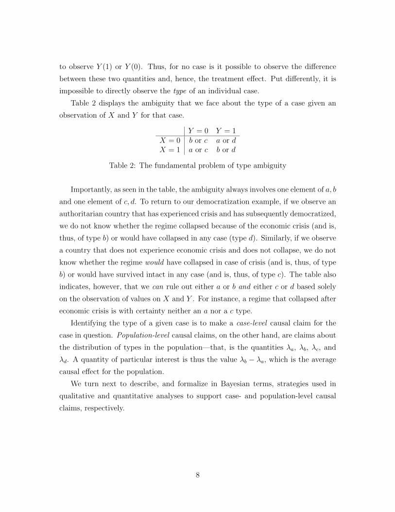
Table 2 displays the ambiguity that we face about the type of a case given an

observation of X and Y for that case.

Y = 0 Y = 1X = 0 b or c a or dX = 1 a or c b or d

Table 2: The fundamental problem of type ambiguity

Importantly, as seen in the table, the ambiguity always involves one element of a, b

and one element of c, d. To return to our democratization example, if we observe an

authoritarian country that has experienced crisis and has subsequently democratized,

we do not know whether the regime collapsed because of the economic crisis (and is,

thus, of type b) or would have collapsed in any case (type d). Similarly, if we observe

a country that does not experience economic crisis and does not collapse, we do not

know whether the regime would have collapsed in case of crisis (and is, thus, of type

b) or would have survived intact in any case (and is, thus, of type c). The table also

indicates, however, that we can rule out either a or b and either c or d based solely

on the observation of values on X and Y . For instance, a regime that collapsed after

economic crisis is with certainty neither an a nor a c type.

Identifying the type of a given case is to make a case-level causal claim for the

case in question. Population-level causal claims, on the other hand, are claims about

the distribution of types in the population—that, is the quantities λa, λb, λc, and

λd. A quantity of particular interest is thus the value λb − λa, which is the average

causal effect for the population.

We turn next to describe, and formalize in Bayesian terms, strategies used in

qualitative and quantitative analyses to support case- and population-level causal

claims, respectively.

8

The process tracing approach

While process tracing can be put to different purposes, we focus here on process

tracing as an approach that draws causal inferences—about whether X caused Y or

how X caused Y—for a given case, by exploiting information from the causal process

thought to connect X and Y or from the context in which that process unfolds.

Typically, the analyst draws on a theoretical causal logic to make predictions about

the within-case evidence that should be observed if a given causal relationship or

mechanism is operating.

Translated into our typological setup, we can summarize the standard view of

process tracing as a method that inspects a case for evidence of that case’s type:

that is, to determine whether or not the outcome in that case was generated by the

case’s treatment status on a given X. We refer to the within-case evidence gathered

during process tracing as clues in order to underline their probabilistic relationship

to the causal relationship of interest. Readers familiar with Collier, Brady, and

Seawright’s (2010) framework can usefully think of our “clues” as akin to causal

process observations, although we highlight that there is no requirement that the

clues be generated by the causal process per se. Process tracing can be understood

as a search for clues that will be observed with some probability if the case is of a

given causal type and that will be observed with some differing probability if the

case is of a different causal type.

It is relatively straightforward to express the logic of process tracing in Bayesian

terms, a step that will aid the integration of qualitative with quantitative causal

inferences. As noted by others (e.g. Bennett (2008), Beach and Pedersen (2013),

Rohlfing (2012)), there is an evident connection between the use of evidence in

process tracing and Bayesian inference. In the paper’s Supplementary Materials

(§A), we provide a survey of recent accounts and applications of process tracing that

follow a logic akin to that underlying our formalization.

In a Bayesian setting, we begin with a prior belief about the probability that

a hypothesis is true. New data then allow us to form a posterior belief about the

probability of the hypothesis.

9

Formally, we express Bayes’ rule as:

Pr(H|D) =Pr(D|H) Pr(H)

Pr(D)(1)

H represents our hypothesis, which may consist of beliefs about one or more

parameters of interest. D represents a particular realization of new data (e.g., a

particular piece of evidence that we might observe). Thus, our posterior belief derives

from three considerations. First, the “likelihood”: how likely are we to have observed

these data if the hypothesis were true, Pr(D|H)? Second, how likely were we to have

observed these data regardless of whether the hypothesis is true or false, Pr(D)? Our

posterior belief is further conditioned by the strength of our prior level of confidence

in the hypothesis, Pr(H). The greater the prior likelihood that our hypothesis is

true, the greater the chance that new data consistent with the hypothesis has in fact

been generated by a state of the world implied by the hypothesis.

In formalizing Bayesian process tracing, we start with a very simple setup, which

we then elaborate. To return to our running example, suppose that we already have

X, Y data on one authoritarian regime: we know that it suffered economic crisis

(X = 1) and collapsed (Y = 1). But what caused the collapse? We answer the

question by collecting one or more clues that we believe are related to the case-level

causal effect of X on Y . We use the variable K to register the outcome of the

search for a clue (or collection of clues), with K=1 indicating that a specific clue (or

collection of clues) is searched for and found, and K=0 indicating that the clue is

searched for and not found.

Bayesian inference involves five steps: (a.) defining our parameters, which are the

key quantities of interest, (b.) stating prior beliefs about the parameters of interest,

(c.) defining a likelihood function, (d.) assessing the probability of the data, and

(e.) the application of Bayes’ rule. We discuss each of these steps, in the context of

process tracing, in turn.

Parameters. For an X = Y = 1 case, the inferential challenge is to determine

whether the regime collapsed because of the crisis (the case is a b type) or whether it

would have collapsed even without it (d type). The parameter of interest is thus the

causal type. Let j ∈ {a, b, c, d} refer to the type of an individual case. Our hypothe-

sis, in this initial setup, consists of a belief about j for the case under examination:

10

specifically whether the case is a b type (j = b). 3

Prior. We then assign a prior degree of confidence to the hypothesis (Pr(H)).

This is, here, our prior belief that an authoritarian regime that has experienced

economic crisis is a b. For now, we express this belief as a prior point probability.

Likelihood. We next indicate the likelihood, Pr(K = 1|H). This is the prob-

ability of observing the clue, when we look for it in our case, if the hypothesis is

true—i.e., here, if the case is a b type. We thus require beliefs relating clues to

causal types.

The key feature of a clue is that the probability of observing the clue is believed

by the researcher to be a function of the case’s causal type. For the present example,

we will need two such probabilities: we let φb denote the probability of observing

the clue for a case of b type (Pr(K = 1|j = b)), and φd the probability of observing

the clue for a case of d type (Pr(K = 1|j = d)). We note that, for the hypothesis

that the case is a b, φb corresponds to Van Evera (1997)’s concept of “certainty.” 4

The key idea in process tracing is that the difference between the probability of the

clue for b type (φb) and for a d type (φd) provides the clue with “probative value,”

— that is, the ability to generate learning about causal types.5

In process tracing, analysts’ beliefs about the probabilities of observing clues for

cases with different causal effects typically derive from theories of, or evidence about,

the causal process connecting X and Y . Suppose we theorize that the mechanism

through which economic crisis generates collapse runs via the regime’s diminished

capacity to reward its supporters. A possible clue to the operation of a causal effect,

then, might be the observation of diminishing rents flowing to regime supporters

shortly after the crisis. Given our theory, this is a clue that we might believe to be

3More formally, we can let our hypothesis be a vector θ that contains a set of indicators for thecausal type of the case γ = (γb, γd), where γj ∈ {0, 1} and

∑γj = 1.

4More fundamentally one might think of types being defined over Y and K as a function ofX. Thus potential clue outcomes could also be denoted K(1) and K(0). High expectations forobserving a clue for a b type then correspond to a belief that many exchangeable units for whichY (X) = X also have K(1) = 1 (whether or not K(0) = 0).

5More formally, we operationalize the concept of probative value in this paper as twice theexpected change in beliefs (in absolute value) from searching for a clue that is supportive of aproposition, given a prior of 0.5 for the proposition. For example, in determining whether j = b orj = d for a given case, starting from a prior of 0.5 and assuming φb > φd, the expected learningcan be expressed as EL = .5(.5φb/(.5φb + .5φd)− .5) + .5(.5− (1− φb).5/((1− φb).5 + (1− φd).5)).The probative value, after simplifying, is then: PV = φb/(φb +φd)− (1−φb)/((1−φb) + (1−φd)),which takes on values between 0 and 1.

11

highly probable for cases of type b that have experienced economic crisis (where the

crisis in fact caused the collapse) but of low probability for cases of type d that have

experienced crisis (where the collapse occurred for other reasons). This would imply

a high value for φb and low value for φd.

Here the likelihood, Pr(K = 1|H), is simply φb.

Note that the likelihood takes account of known features of the data-gathering

process. The likelihood given here is based on the implicit assumption that the case

is randomly sampled from a population of X = Y = 1 cases for which share φb of

the b cases have clue K = 1 and share φd of the d cases have clue K = 1.

Probability of the data. This is the probability of observing the clue when we

look for it in a case, regardless of its type, (Pr(K = 1)). More specifically, it is the

probability of the clue in a treated case with a positive outcome. As such a case can

only be a b or a d type, this probability can be calculated simply from φb and φd,

together with our beliefs about how likely an X = 1, Y = 1 case is to be a b or a d

type. This probability aligns (inversely) with Van Evera’s concept of “uniqueness.”

Inference. We can now apply Bayes’ rule to describe the learning that results

from process tracing. If we observe the clue when we look for it in the case, then our

posterior belief in the hypothesis that the case is of type b is:

Pr(j = b|K = 1) =Pr(K = 1|j = b) Pr(j = b)

Pr(K = 1)=

φb Pr(j = b)

φb Pr(j = b) + φd Pr(j = d)

Suppose, in our running example, that we believe the probability of observing

the clue for a treated b case is φb = 0.9 and for a treated d case is φd = 0.5, and that

we have prior confidence of 0.5 that an X = 1, Y = 1 case is a b. We then get:

Pr(j = b|X = Y = K = 1) =0.9× 0.5

0.9× 0.5 + 0.6× 0.5= 0.6

Analogous reasoning follows for process tracing in cases with other X, Y values.

For an X = 0, Y = 1 case, for instance, we need prior beliefs about whether the case

is an a or a d type and beliefs about the probabilities φa and φd for the clue being

sought.

12

The inferential leverage in process tracing thus comes from differences in the

probability of observing K = 1 for different causal types. As should also be clear, the

logic described here generalizes Van Evera’s familiar typology of tests by conceiving

of the certainty and uniqueness of clues as lying along a continuum.

Van Evera’s four tests (“smoking gun,” “hoop,” “straw in the wind,” and “dou-

bly decisive”) represent, in this sense, special cases—particular regions near the

boundaries of a “probative-value space.” To illustrate, we represent the range of

combinations of possible probabilities for φb and φd as a square in Figure 1 and mark

the spaces inhabited by Van Evera’s tests. As can be seen, the type of test involved

depends on both the relative and absolute magnitudes of φb and φd. Thus, a clue

acts as a “smoking gun” for proposition “b” (the proposition that the case is a b

type) if it is highly unlikely to be observed if proposition “b” is false, and more likely

to be observed if the proposition is true (bottom left, above diagonal). A clue acts

as a “hoop” test if it is highly likely to be found if “b” is true, even if it still quite

likely to be found if it is false. Doubly decisive tests arise when a clue is very likely if

“b” and very unlikely if not. It is also easy to imagine clues with probative qualities

lying in the large space amidst these extremes.

At the same time, the probative value of a test does not fully describe the learning

that takes place upon observing evidence. Following Bayes’ rule, inferences also

depend on our prior confidence in the hypothesis being tested. At very high or very

low levels of prior confidence in a hypothesis, for instance, even highly probative

evidence has minimal effect on posteriors; the greatest updating generally occurs

when we start with moderate prior probabilities. Figure 5 in the Supplementary

Materials (§B) graphically illustrates the effect of prior confidence on learning.

We have so far described a very simple application of Bayesian logic. A further

elaboration, however, can place process tracing in a more fully Bayesian setting,

allowing for considerable gains in learning. Instead of treating clue probabilities (φ

values) as fixed, we can treat them as parameters to be estimated from the data.

In doing so, we allow the search for clues to provide leverage not only on a case’s

type but also, given a belief about type, on the likelihood that a case of this type

generates the clue. We can define our hypothesis as a vector, θ, that includes both

the causal type of the case and the relevant φ values, e.g., φb, φd. We can then

13

0.0 0.2 0.4 0.6 0.8 1.0

0.0

0.2

0.4

0.6

0.8

1.0

Classification of tests

φd (Probability of observing K given d)

φ b (

Pro

babi

lity

of o

bser

ving

K g

iven

b)

K present: doubly decisive for b

K absent: doubly decisive for d

K present: smoking gun for b

K absent hoop test for d

K present: hoop test for b

K absent: smoking gun for d

K present: straw in the wind for b

K absent: straw in the wind for d

K present: doubly decisive for d

K absent: doubly decisive for b

K present: hoop test for d

K absent: smoking gun for b

K present: smoking gun test for d

K absent: hoop test for b

K present: straw in the wind for d

K absent: straw in the wind for b

More sensitive for b

More specific for b

More specific for d

More sensitive for d

Figure 1: A mapping from the probability of observing a clue if a proposition ”b”(i.e., that a case is a b type) is true (φb) or false (φd) to a generalization of the testsdescribed in Van Evera (1997).

define our prior as a prior probability distribution p(θ) over θ.6 We can thus express

any prior uncertainty about the relationship between causal effects and clues. Our

likelihood is then a function that maps each possible combination of type and the

relevant φ values to the probability of observing the clue when we search for it, given

6Here, this distribution could, for example, be given by the product of a categorical distributionover γ (indicators of causal type) and a Beta distribution for each φj .

14

those parameter values.

In this multi-parameter approach, updating produces a joint posterior distribu-

tion over type and our φ values. Observing the clue will shift our posterior in favor of

type and φ-value combinations that are more likely to produce the clue. In sum, and

critical to what follows, we can simultaneously update beliefs about both the case’s

type and the probabilities linking types to clues—learning both about causal effects

and empirical assumptions. We provide further intuition on, and an illustration of,

this elaboration in the Supplementary Materials (§B).

The correlational approach

The correlational solution to the fundamental problem of causal inference is to focus

on population-level effects. Rather than seeking to identify the types of particular

cases, researchers exploit covariation across cases between the treatment and the

outcome variables—i.e., dataset observations—in order to assess the average effect

of treatment on outcomes for a population or sample of cases.

In the simplest, frequentist approach, under conditions described by Rubin (1974),

the average effect of a treatment may be estimated as the difference between the av-

erage outcome for those cases that received treatment and the average outcome for

those cases that did not receive treatment.

Although this frequentist approach to estimating causal effects from correlational

data is more familiar, recasting the strategy in Bayesian terms will facilitate the

integration of within-case and between-case data that we undertake below. The

general utility of the Bayesian framework for cross-case data analysis is already well

appreciated, and so we simply review Bayesian correlational inference as applied to

the binary setup around which this paper is structured.7

Suppose, returning to our running example, that we are interested in determining

the distribution of causal types in a population of authoritarian regimes. We again

need to specify our parameters, priors, likelihood, and the probability of the data,

and then draw our inference via the application of Bayes’ rule:

Parameters. One set of parameters to be estimated are our λ values: i.e., the

7For a similar treatment for a case with known propensities but non-compliance see Imbens andRubin (1997).

15

proportion of the population of authoritarian regimes for which economic crisis would

prevent collapse (λa); the proportion for which it would cause collapse (λb); and so

on.

As in our multi-parameter process-tracing setup, we also include a set of param-

eters capturing analytic assumptions. In correlational inference, these parameters

relate to the process of assignment of types to treatment. Let πj denote the (possi-

bly unknown) probability that a case of type j is assigned to treatment (X = 1).8

Thus, for instance, πb indicates the likelihood that a country of type b (one sus-

ceptible to a regime-collapsing effect of crisis) has been “assigned” to experiencing

economic crisis. Critically, the X, Y data pattern consistent with any given belief

about the distribution of types depends on beliefs about the assignment probabilities.

We can now define our hypothesis as a vector, θ = (λa, λb, λc, λd, πa, πb, πc, πd),

that registers a possible set of values for the parameters over which we will update:

type proportions in the population and assignment propensities by type.

Prior. We next need to assign a prior probability to θ. In the general case, we

will do so by defining a prior probability distribution, p(θ), over possible values of

the elements of θ.

Likelihood. Our data, D, consist of X and Y observations for a sample of cases.

With a binary X and Y , there are four possible data realizations (combinations

of X and Y values) for a given case. For a single case, it is straightforward to

calculate an event probability wxy — that is, the likelihood of observing the particular

combination of X and Y given the type shares and assignment probabilities in θ.

For instance:

w00 = Pr(X = 0, Y = 0|θ) = λb(1− πb) + λc(1− πc) (2)

More generally, let wXY denote the vector of these event probabilities for each

combination of X and Y values, conditional on θ. Further, let nXY denote a vector

containing the number of cases observed with each X, Y combination and n the

total number of observed units. Under an assumption of independence (data are

independently and identically distributed), the full likelihood is then given by the

8We assume that all cases are independently assigned values on X.

16

multinomial distribution:

Pr(D|θ) = Multinomial(nXY |n,wXY )

We again assume here that cases are randomly drawn from the population, though

more general functions can allow for more complex data gathering processes.

Probability of the data. We calculate the unconditional probability of the

data, Pr(D), by integrating the likelihood function above over all parameter values,

weighted by their prior probabilities.

Inference. After observing our data, D, we then form posterior beliefs over θ

by direct application of Bayes’ rule, above:

p(θ|D) =Pr(D|θ)p(θ)∫

Pr(D|θ′)p(θ′)dθ′(3)

This posterior distribution reflects our updated beliefs about which sets of pa-

rameter values are most likely, given the data. Critically, upon observing X and Y

data, we simultaneously update beliefs about all parameters in θ: beliefs about causal

effects (type shares) in the population and beliefs about the assignment propensities

for cases of each type. We provide further detail and a simple illustration in the

Supplementary Materials (§C).

Bayesian Integration of Qualitative and Quantita-

tive data

We now turn to the unification of Bayesian inference from correlational and process-

tracing data. As described above, a Bayesian approach can be used to update beliefs

about causal effects using either process-based or correlational data. The BIQQ

framework builds on this logic to allow updating of causal beliefs and analytic as-

sumptions following the observation of any combination of X, Y data and within-case

clues.

The basic intuition of the BIQQ approach is as follows. Observations of X and

Y values for a case provide some discriminating information about the type of that

17

case—in our binary setup, narrowing it down to one of two types. (For instance,

an X = 1, Y = 1 case can only be a b or a d.) Additional within-case clue (K)

information provides further discriminating power. Put another way, since the causal

type affects the likelihood of observing patterns over X, Y , and K, information about

all three of these quantities allows us to update over the causal types.

Critically, however, beyond providing a way to update over the distribution of

causal types, BIQQ produces a set of updated beliefs about other quantities such

as assignment processes and the probative value of clues. Moreover, while we focus

here on inference regarding average causal effects, the same framework can be used

to generate updated beliefs about case-level explanations or about theoretical logics

(e.g., theories of mechanism).

We emphasize that the BIQQ framework’s critical integrative move derives from

writing down a likelihood function that maps each point in the parameter space onto

the probability of occurrence of the observed pattern of quantitative and qualitative

data. While we place estimation in a Bayesian framework, thus allowing for inte-

gration of prior knowledge about the parameters, the basic approach might also be

implemented in a non-Bayesian, maximum-likelihood setting, as we discuss in the

Supplementary Materials (§J).

In the remainder of this section we describe a simple but complete baseline model

that is likely to cover a range of applications of interest. We then discuss how this

basic model can be extended to more complex research situations.

Baseline Model

Turning now to the formalization of the baseline model, we describe a complete

BIQQ model with respect to parameters, priors, likelihood, and inference.

Parameters

In the baseline model, we have three sets of parameters:

1. The population distribution of causal types

2. The probabilities with which types are assigned to treatment

18

3. The probabilities with which clues are associated with types

We discuss these in turn.

Distribution of types. As above, we are interested in the proportion of a, b,

c, or d types in the population, denoted by λ = (λa, λb, λc, λd) (Table 1). Implicit

in this representation of causal types is a SUTVA assumption — i.e., that potential

outcomes for a given case depend only on that case’s treatment status. Our setup

with four types also implies just a single explanatory variable. Though embedded in

the baseline model, both assumptions can be relaxed (see discussion of extensions,

below).

Treatment assignment. Let π = (πa, πb, πc, πd) denote the collection of as-

signment probabilities: that is, the probability of receiving treatment (X=1) for

cases of each causal type. We assume in the baseline model that cases are indepen-

dently assigned to treatment. Assignment propensities could in principle, however,

be modeled as correlated or as dependent on covariates.

Clues. Let φ = (φjx) denote the collection of probabilities that a case of

type j will exhibit clue K = 1 (when it is sought), when X = x. Thus, φb1 is

the probability of observing the clue for a treated case of b type, while φb0 is the

probability of observing the clue for an untreated b type. Note that we allow clue

probabilities to be conditional on a case’s treatment status. The rationale is that,

for many process-based clues, their likelihood of being observed will depend on the

case’s causal condition. We again assume that the realization of clues is independent

across cases. For simplicity, we write down the baseline model in terms of the search

for a single clue, though a search for multiple clues can readily be accommodated.

In total, in the baseline model the parameter vector θ has 16 elements grouped

into three families: θ = (λ, π, φ).

Priors

Our uncertainty before seeing the data is represented by a prior probability dis-

tribution over the parameters of interest, given by p(θ). The model accords great

flexibility to researchers in specifying these prior beliefs, a point we return to in the

concluding section. In our baseline model, we employ priors formed from the product

of priors over the component elements of θ; that is, we assume that priors over pa-

19

rameters are independent. For the λ parameters, we employ a Dirichlet distribution

in most applications below; for π and φ parameters, we employ a collection of Beta

distributions.

In some situations, researchers may have uncertainty over some parameters but

know with certainty the value of others. In experimental work, for instance, assign-

ment probabilities may be known with certainty. Parameters with known values can

be removed from θ, entering into the likelihood as fixed values. We model φ as fixed

in some applications below; in general, we expect researchers to have uncertainty

over λ and φ and, in most observational work, over π as well.

Sharper (lower-uncertainty) priors on one set of parameters can generate more

learning about the others. For instance, we can learn more about causal effects and

clue probabilities when we have sharper priors on assignment propensities.

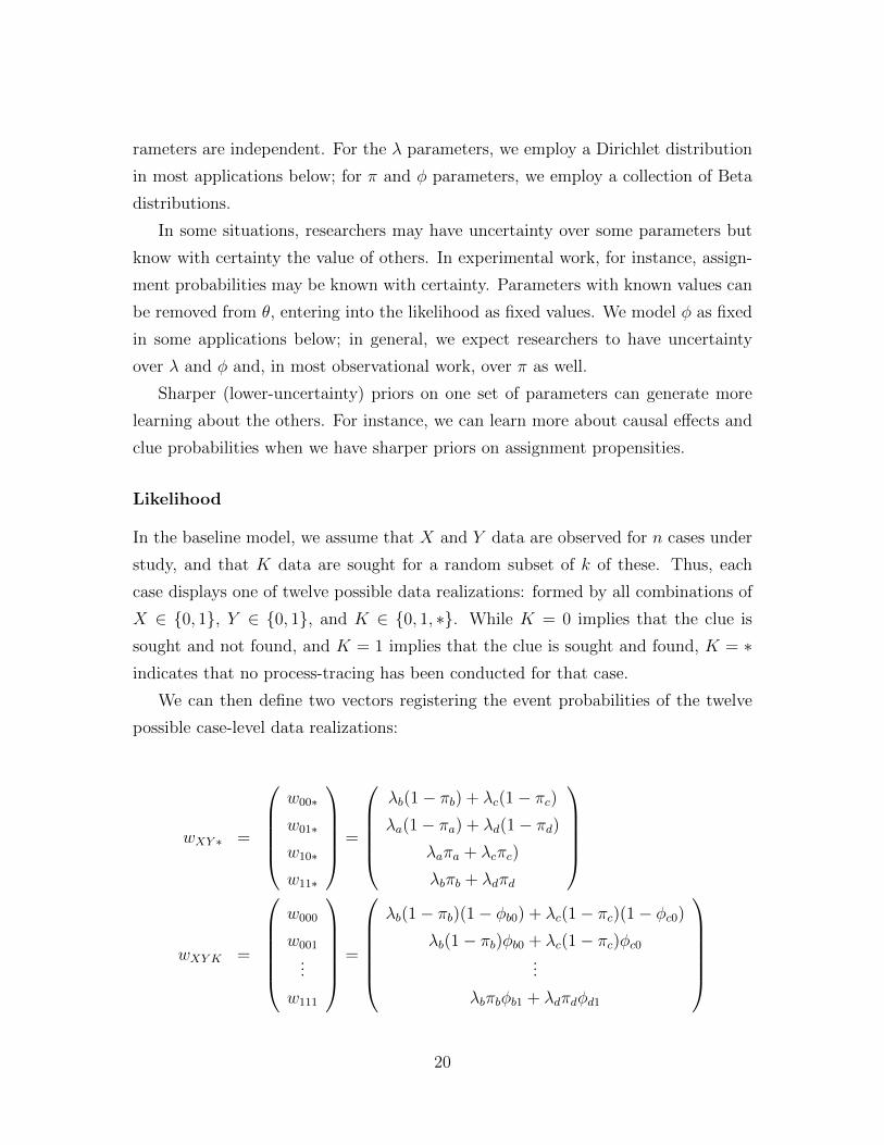
Likelihood

In the baseline model, we assume that X and Y data are observed for n cases under

study, and that K data are sought for a random subset of k of these. Thus, each

case displays one of twelve possible data realizations: formed by all combinations of

X ∈ {0, 1}, Y ∈ {0, 1}, and K ∈ {0, 1, ∗}. While K = 0 implies that the clue is

sought and not found, and K = 1 implies that the clue is sought and found, K = ∗indicates that no process-tracing has been conducted for that case.

We can then define two vectors registering the event probabilities of the twelve

possible case-level data realizations:

wXY ∗ =

w00∗

w01∗

w10∗

w11∗

=

λb(1− πb) + λc(1− πc)λa(1− πa) + λd(1− πd)

λaπa + λcπc)

λbπb + λdπd

wXYK =

w000

w001

...

w111

=

λb(1− πb)(1− φb0) + λc(1− πc)(1− φc0)

λb(1− πb)φb0 + λc(1− πc)φc0...

λbπbφb1 + λdπdφd1

20

We next let nXYK denote an 8-element vector recording the number of cases in

a sample displaying each possible combination of X, Y,K data, where K ∈ {0, 1},thus: nXYK = (n000, n001, n100, . . . , n111). The elements of nXYK sum to k. Similarly,

we let nXY ∗ denote a four-element vector recording the data pattern for cases in

which no clue evidence is gathered: nXY ∗ = (n00∗, n01∗, n10∗, n11∗), with the elements

summing to n − k. Finally, assuming that data are independently and identically

distributed, the likelihood is:

Pr(D|θ) = Multinom (nXY ∗|n− k, wXY ∗)×Multinom (nXYK |k, wXYK)

This likelihood simply records the product of the probability that X, Y data

would look as they do in those cases in which only X, Y data are gathered (given the

number of such cases and the event probability associated with each possible X, Y

data realization), and the probability that the X, Y,K data would look as they do

in those cases in which within-case data are also gathered (given the number of such

cases and the event probability for each possible X, Y,K data realization).

As before, we highlight that the likelihood contains information on data gathering:

in particular, on qualitative and quantitative case selection. The baseline model

assumes that clue evidence is sought in a randomly selected set of cases. Again, one

could model more complex qualitative case selection processes, which for instance

might be independent (if for example a clue is sought in each case with a fixed

probability), dependent on X or Y values, or dependent on potential outcomes. We

discuss these possibilities in the Supplementary Materials (§F).

Further, the baseline model assumes that the overall number of studied cases is

fixed at n and that each case is selected for study with equal probability. Alterna-

tively, one could model the probability of selection of cases as independent (and thus

the number of cases, n, as stochastic) or as dependent on potential outcomes or other

features (such as the values of X or Y ). Some of these possibilities are addressed in

the Supplementary Materials (§F). Our application below to the civil-war literature

also illustrates how known non-random case selection processes can sometimes be

treated as random, conditional on a clue.

The assumption of random sampling in the baseline model, both for the selection

of study cases (from the population) and for the selection of a subsample of these

21

for further, within-case data collection, justifies treating cases as “exchangeable,”

which renders the likelihood function informative (Ericson, 1969). More generally,

even where researchers choose to sample on some observable (e.g., X or Y values),

selecting randomly (conditional on that observable) will generally be necessary to

defend an assumption of exchangeability.

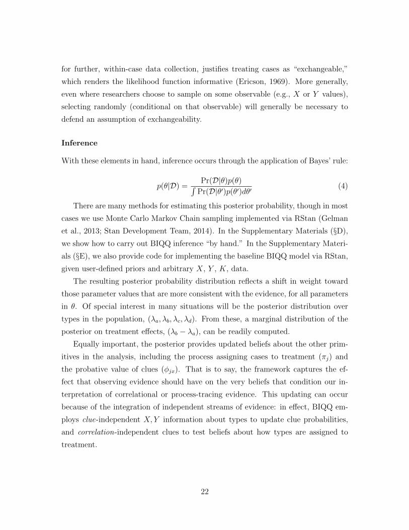
Inference

With these elements in hand, inference occurs through the application of Bayes’ rule:

p(θ|D) =Pr(D|θ)p(θ)∫

Pr(D|θ′)p(θ′)dθ′(4)

There are many methods for estimating this posterior probability, though in most

cases we use Monte Carlo Markov Chain sampling implemented via RStan (Gelman

et al., 2013; Stan Development Team, 2014). In the Supplementary Materials (§D),

we show how to carry out BIQQ inference “by hand.” In the Supplementary Materi-

als (§E), we also provide code for implementing the baseline BIQQ model via RStan,

given user-defined priors and arbitrary X, Y , K, data.

The resulting posterior probability distribution reflects a shift in weight toward

those parameter values that are more consistent with the evidence, for all parameters

in θ. Of special interest in many situations will be the posterior distribution over

types in the population, (λa, λb, λc, λd). From these, a marginal distribution of the

posterior on treatment effects, (λb − λa), can be readily computed.

Equally important, the posterior provides updated beliefs about the other prim-

itives in the analysis, including the process assigning cases to treatment (πj) and

the probative value of clues (φjx). That is to say, the framework captures the ef-

fect that observing evidence should have on the very beliefs that condition our in-

terpretation of correlational or process-tracing evidence. This updating can occur

because of the integration of independent streams of evidence: in effect, BIQQ em-

ploys clue-independent X, Y information about types to update clue probabilities,

and correlation-independent clues to test beliefs about how types are assigned to

treatment.

22

Extensions

The baseline model simplifies certain features of real-world research situations: treat-

ments and outcomes are binary; neither measurement error nor spillovers occur; there

is only one treatment of interest and one clue to examine; and our focus is on a single

causal estimand (population-level treatment effects).

Importantly, however, the basic logic of integration underlying the BIQQ frame-

work does not depend on any of these assumptions. In what follows, we suggestively

indicate how BIQQ can be extended to capture a wider range of research situations

and objectives.

Multiple explanatory variables and interaction effects

Suppose that, instead of a single explanatory variable, we have m explanatory (or

control) variables X1, X2, . . . , Xm. As these m variables can take on 2m possible

combinations of values, we now have 22m types, rather than four. Assuming that clue

probabilities are conditional on type and the values of the explanatory variables, φ

would contain 22m × 2m = 22m+m rather than the eight values in our baseline model.

In the Supplementary Materials (§F), we describe the situation with two explanatory

variables in more detail and show how this setup allows researchers to examine both

interaction effects and equifinality.

Continuous data

We can similarly shift from binary to continuous variable values through an expan-

sion of the set of causal types. Suppose that Y can take on m possible values.

With k explanatory variables, each taking on r possible values, we then have mrk

causal types and, correspondingly, very many more elements in φ. Naturally, in

such situations, researchers might want to reduce complexity by placing structure

onto the possible patterns of causal effects and clue probabilities, such as assuming

a monotonic function linking effect sizes and clue probabilities.

23

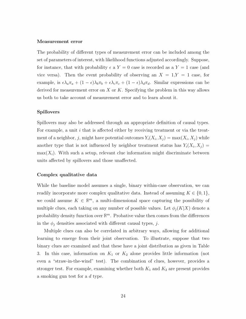
Measurement error

The probability of different types of measurement error can be included among the

set of parameters of interest, with likelihood functions adjusted accordingly. Suppose,

for instance, that with probability ε a Y = 0 case is recorded as a Y = 1 case (and

vice versa). Then the event probability of observing an X = 1,Y = 1 case, for

example, is ελaπa + (1 − ε)λbπb + ελcπc + (1 − ε)λdπd. Similar expressions can be

derived for measurement error on X or K. Specifying the problem in this way allows

us both to take account of measurement error and to learn about it.

Spillovers

Spillovers may also be addressed through an appropriate definition of causal types.

For example, a unit i that is affected either by receiving treatment or via the treat-

ment of a neighbor, j, might have potential outcomes Yi(Xi, Xj) = max(Xi, Xj) while

another type that is not influenced by neighbor treatment status has Yi(Xi, Xj) =

max(Xi). With such a setup, relevant clue information might discriminate between

units affected by spillovers and those unaffected.

Complex qualitative data

While the baseline model assumes a single, binary within-case observation, we can

readily incorporate more complex qualitative data. Instead of assuming K ∈ {0, 1},we could assume K ∈ Rm, a multi-dimensional space capturing the possibility of

multiple clues, each taking on any number of possible values. Let φj(K|X) denote a

probability density function over Rm. Probative value then comes from the differences

in the φj densities associated with different causal types, j.

Multiple clues can also be correlated in arbitrary ways, allowing for additional

learning to emerge from their joint observation. To illustrate, suppose that two

binary clues are examined and that these have a joint distribution as given in Table

3. In this case, information on K1 or K2 alone provides little information (not

even a “straw-in-the-wind” test). The combination of clues, however, provides a

stronger test. For example, examining whether both K1 and K2 are present provides

a smoking gun test for a d type.

24

Type K1 = K2 = 0 K1 = 1, K2 = 0 K1 = 0, K2 = 1 K1 = K2 = 1 Totalb 0 1/2 1/2 0 1d 1/4 1/4 1/4 1/4 1

Table 3: Clue distribution for types b and d (given X = 1). Cells show the probabilityof a given clue combination for each causal type.

Evaluating theories

The framework can also be used to keep track of uncertainty over the validity of a

theory (e.g., a theory of causal mechanism) underlying a set of clue predictions. Let

ηt ∈ {0, 1} denote the event that theory t, specifying a particular causal mechanism,

is correct. We can allow for uncertainty over t by including ηt in our vector of

parameters of interest, θ, and our confidence in t is then captured by p(θ). Although

ηt is never directly observed, we may associate different theories with the presence or

absence of different clues in different X, Y conditions, or with distributions of causal

types. Beliefs in t can thus be updated as we observe patterns in the data. In our

running example above, suppose that we expect a clue—say, diminishing rents—to be

more likely to be observed in b cases facing crisis than in d cases. If we then observe

the clue more frequently in cases that have X, Y values that are more consistent

with a b than a d type, the result will be an increase in the weight accorded to

theory t, from which the clue predictions for differentiating b from d types have been

derived. In associating clue patterns with theories in this way, our framework allows

for simultaneous learning about the probative value of clues and about the validity

of different theoretical accounts of causal processes. We give an illustration of this

logic in the Supplementary Materials (§D).

Other variations might allow for different forms of effect heterogeneity, or for

different case-selection strategies.

Illustrations of the BIQQ approach

We provide two illustrations of the BIQQ approach. In each case we combine quanti-

tative and qualitative data generated by different scholars to address major questions

in political economy: the origins of electoral systems and the causes of civil wars.

25

Application 1: The Origin of Electoral Systems

We now apply the BIQQ framework to an issue that has received both quantitative

and qualitative treatment in comparative politics: explaining variation in electoral

systems across democracies. We use this application in part to illustrate the sub-

stantive effects that integration can have on causal conclusions. Equally important,

the application demonstrates the dependence of conclusions on how many and which

cases are selected for qualitative analysis.

Boix (1999) advances one influential theory of electoral-system choice as well as

a quantitative test of the theory. In brief, Boix theorizes that the preferences of gov-

erning parties between plurality rules and proportional representation (PR) depend

on the threat posed by challenger parties under the current rules. In particular, the

presence of a strong opposition party together with coordination failure among the

ruling parties will create strong incentives for governments to shift from plurality

to PR. Boix’s central test of the theory focuses on a set of 22 interwar European

cases. In this context—following the extension of universal suffrage, enabling the

rise of socialist challengers—the theory implies that ruling parties should have been

most likely to shift to PR where the left was electorally strong and the right was

fragmented. In his main model, Boix regresses the effective electoral threshold on

the electoral strength of the left, the effective number of right parties, the interaction

of the two, and a number of controls, and finds (consistent with the theory) a strong

negative interaction between left strength and right division.

Kreuzer (2010) then undertakes a qualitative analysis of Boix’s cases. He does so

by collecting within-case information relating to three implications of Boix’s causal

logic. For each case, Kreuzer asks: 1.) whether any proposal for PR followed a

major suffrage expansion, 2.) whether it was ruling parties who initiated move, and

3.) whether the ruling parties were united in their support for PR. Kreuzer reports

that the process-tracing yields full support for the theory in 36 percent of the cases,

partial support in 21 percent, and no support in the remaining cases.

What conclusion can be drawn from the adjoining of these two analyses? Kreuzer

draws the reasonable inference that Boix’s theory offers an incomplete explanation

of PR adoption. Yet it is not at all obvious how much this particular mix of con-

firmatory and disconfirmatory qualitative evidence should unsettle the quantitative

26

Y = 0 Y = 1X = 0 K = 0 4 3

K = 1 0 1X = 1 K = 0 1 7

K = 1 0 4

Table 4: Data used for Boix-Kreuzer analysis

findings. That is, it is not clear what these two separate analyses—one quantitative,

the other qualitative—ought to imply for our beliefs about the effect of left threat

on PR adoption in interwar Europe. The separated analyses also do not allow us

to learn about other parameters of interest, such as the distribution of case types,

the probative value of the clues, or the propensities of different types of cases to be

assigned to treatment.

We illustrate how BIQQ can be applied to a somewhat simplified version of

the problem, focusing on the average causal effect of left threat as our estimand of

interest. Consistent with the setup introduced above, we treat all variables as binary,

employing the dichotomized codings of Boix’s independent and dependent variables

as provided in Table 5 of Kreuzer (2010). Since the move to PR is theorized to

depend both on the left being strong and the right being divided, we code a single

independent variable, X, as 1 if and only if Kreuzer codes both conditions as present

and 0 otherwise. We include in the analysis only those cases that started with single-

member districts, thus dropping 2 of Boix’s cases. And we code Y as 1 if the country

moved to a form of PR and 0 otherwise.9 Further, we maintain the bivariate setup

for the correlational analysis, setting aside the covariates in Boix’s analysis. We note

that, even with these simplifications, the basic bivariate relation between X and Y

remains consistent with Boix’s theory and strong (correlation = 0.47, p = 0.036).

Finally, we collapse Kreuzer’s three process-tracing tests into a single clue. We

code the clue K=1 for a given case if all three clues are present and K=0 if one or

more of the indicators is absent.

Table 4 summarizes the X, Y , and clue (K) data that enter into the analysis,

indicating the number of cases with each combination of X, Y , and K values.

Alongside the data given in Table 4, we need to supply priors or known values on

9As our purpose is to illustrate the integration that BIQQ enables, rather than to weigh in onthe substantive debate, we do not seek to adjudicate Kreuzer’s coding choices.

27

the parameters of interest: the distribution of types (a, b, c, and d) in the population;

the probability of each type being assigned to treatment; and the probative value of

clues. In this exercise, we fix assignment propensities to 0.5 for a and b types but

use a flat prior for the assignment of c and d types.10 We employ a flat Dirichlet

distribution for the proportion of each type in the population.

Finally, while Kreuzer does not indicate the probative value he assumes for his

clues, we assign probabilities of observing the clues for each type and treatment

status by reasoning with Boix’s theoretical framework. For this analysis we assume

no uncertainty over the probative value of clues, fixing the eight φ parameter values.

The specific φ values that we employ and our detailed reasoning can be found in the

Supplementary Materials (§G.1). Among the more important φ probabilities here

are those associated with b and d types for cases with X = 1 values. For cases with

high left threat and a shift to PR, the inferential task is to determine whether they

would have (d) or would not have (b) shifted to PR without left threat. The φb1 and

φd1 values that we have chosen are such that the clue operates as a hoop test for the

proposition that such a case is a b type. On the other hand, for cases with no left

threat and no shift to PR (which could be b or c types), φ values are such that the

search for Kreuzer’s clue will be minimally informative. This is because, regardless

of type, the theory would not expect ruling parties to unanimously push for PR in

the absence of left threat. Off the diagonal, in low-threat cases that shifted to PR,

the φ probabilities make the clue a smoking gun for designation as a d type; and for

high-threat cases that did not shift, the clue serves as a hoop test for designation as

an a type.

We present the results of the analysis in Figure 2. The figure displays the es-

timated causal effects for a range of possible research strategies. All strategies ex-

amined use the correlational data for all 20 cases, but they differ in the number of

cases (k) for which clues are sought. We assume for this analysis that researchers

randomly select the set of cases for which they gather within-case data, giving rise

to a distribution of posterior distributions for each design. The X axis indicates the

number of cases for which clues are sought, while the Y axis reports the resulting

distribution of the posterior expected value of the average causal effect. On the far

10Specifically, we use a flat prior for πc and set πd equal to 1− πc.

28

left, where we employ only Boix’s correlational data and no within-case data, we

estimate a posterior mean just over 0.3. On the far right we see the analysis where

all cases are examined, which yields a posterior mean just below 0.15. Between these

extremes we see the distribution of estimated effects for each design, representing

the causal-effect estimates for 500 random samples of cases for each research design.

Three features of the graph are of particular interest. The results indicate, first,

that the impact of Kreuzer’s full analysis, under our stipulated priors, is large: al-

though it does not eliminate the effect, it cuts the estimated impact of left threat

on electoral-system reform roughly in half. Second, we see that in designs in which

clue data are not collected for all cases, the results depend substantially on which

cases are selected for process tracing. Even with as many as 12 cases, there are

samples that result in a higher estimate of the causal effect than is found in the pure

correlational analysis. Third, we note how slowly the effect of process-tracing data

cumulates as the qualitative sample size increases. If we collect clues on a sample of

the size typical of much qualitative work—say, between 1 and 4 cases—the expected

result moves us no more than about a quarter of the way toward the full 20-case find-

ing. Moreover, with random sampling at least, the variance in estimates resulting

from qualitative samples of this size is large. These findings are all the more striking

given that the clue data are on the whole in substantial tension with Boix’s claims,

that the clues have been assumed to have fairly high probative value, and that the

correlational sample is itself quite small.

Application 2: Natural Resources and Conflict

Our second substantive application focuses on the relationship between natural re-

sources and civil conflict. This application illustrates the use of multiple clues, shows

how conclusions can be reported conditional on beliefs about priors, and highlights

an important feature of integration: that even strongly probative within-case evi-

dence collected for a small number of cases may make only a small contribution to

inference when combined with a substantial amount of correlational data.

We base our analysis on Ross (2004), who undertakes qualitative analyses of

thirteen cases that feature both high levels of natural resources and the emergence of

civil conflict. Ross draws his population of cases from a frame used in a quantitative

29

0 5 10 15 20

0.0

0.1

0.2

0.3

0.4

k : number of cases for which clue data is gathered

Est

imat

ed tr

eatm

ent e

ffect

●

●

●

●

●●

●●

●●

●●

●●

● ● ● ● ● ● ●

Figure 2: Each point represents the mean of the posterior distribution for the averagetreatment effect from a research design in which a random k of 20 available cases arestudied intensively. The black circle marks the mean estimate for each k; for each k,95% of the simulations lie along the black line.

study by Collier and Hoeffler (2004). Ross’s study identifies all cases of civil wars that

started or were ongoing between 1990 and 2000 for which “scholars, nongovernmental

organizations, or UN agencies suggested that natural resource wealth, or natural

resource dependence, influenced the war’s onset, duration, or casualty rate.”11 In

his analysis he seeks evidence of whether natural resources were associated with

looting, grievance, or separatism; on examination of the cases, he also concludes that

foreign intervention and evidence of resource-based rebel financing are also clues for

a causal link between resources and conflict onset. Ultimately, Ross’s determination

of whether natural resources have a causal effect is based on whether any of the

above clues were observed in these cases. In the event, at least one such clue is found

in 5 cases out of the 13 in which clues are sought.

Ross’s overall conclusion is that “in these thirteen conflicts, there is strong evi-

11Although Ross examines onset, duration, and severity, here we focus on onset only.

30

dence that resource wealth has made conflict more likely to occur.” This conclusion

is consistent with the claim in Collier and Hoeffler (2004) that resources are causally

linked to conflict, though Ross’s analysis does not support the interpretation favored

by Collier and Hoeffler. For this analysis, we do not call into question any of Ross’s

conclusions about these cases. We focus instead on assessing the inferences that one

can make from these cases, in combination with the correlational data, about average

causal effects in the population.

Note that Ross’s analysis shares many of the characteristics of the type of qualita-

tive analysis described above. He focuses on a binary outcome variable — war onset

—. Although the underlying treatment variable — natural-resource dependence —

is continuous, he dichotomizes the variable, considering natural resources to be ei-

ther present or absent in each case. Most importantly, Ross’s analysis does not focus

on variation in X and Y to make inferences on causal effects; in fact, only cases

with X = Y = 1 are examined. Inferential leverage is based instead on additional

within-case information — clues — and indeed ultimate conclusions are based on a

single clue, albeit a complex one, for each case: the presence of one of a number of

“subclues,” each of which is indicative of a possible mechanism connecting resources

to war onset.

Qualitative analysts frequently seek to use findings from a sample of this kind to

shed light on broader causal theories. How, then, do Ross’s findings in these 13 case

studies—together with the correlational evidence from Collier and Hoeffler—add up

to a set of population-level causal inferences?

To carry out this integration in the BIQQ framework, we need first to be able

to identify the quantitative sample from which Ross draws his cases. For reasons

that we explain in the Supplementary Materials (§G.2), we identify this sample as

all cases in which there was not a conflict ongoing in the 1990s. Surprisingly, in

this subset of cases the positive relation between X and Y , identified in Collier and

Hoeffler’s study, is not present; indeed there is a small negative negative correlation.

Second, we need to situate the cases in Ross’s qualitative analysis within this

quantitative sample. An important feature of Ross’s analysis is that selection into

the process-tracing sample depends not simply on values of X and Y but also on

expert assessments of whether X and Y are causally linked.12 This implies non-

12Other considerations regarding the sample and the subsample of Ross’s sample that we examine

31

random selection of cases into the process-tracing sample. In our framework, we can

take account of this non-random selection by treating expert statements that natural

resources caused a conflict as a first clue, K1: these statements can be conceptualized

as evidence suggesting that a case is a b type rather than a d type. We can then

conceive of the evidence uncovered in Ross’s own analysis as a second clue, K2, which

is gathered only conditional upon observation of the first clue (and which may or

may not reflect the same underlying information used to generate the first clue).

Employing this interpretation, Table 5 shows the distribution over X, Y,K1, K2

values used in this analysis. Note that there are no K2 data for cases with K1 =

0 (given Ross’s selection rule), and there are only K1 data for cases with X =

Y = 1 (since Ross uses expert causal assessments only of those cases with resources

that experienced wars). This non-rectangularity presents no special problem for the

analysis, however.

Y = 0 Y = 1 K2 = NA K2 = 0 K2 = 1X = 0 61 6 K1 = 0 1X = 1 64 5 K1 = 1 1 3

Table 5: Data on natural resources and conflict. Left panel shows X, Y data basedon Collier and Hoeffler (2004); right panel shows K1, K2 data for cases with X =1, Y = 1, drawn from Ross (2004).

Alongside the data given in Table 5, we need to form priors about the probative

value of clues and about the assignment process. For the purposes of this analysis,

we adopt the positions taken implicitly by Collier and Hoeffler for the X, Y data: we

assume that assignment probabilities are similar for all types — though we allow for

uncertainty over these assignment probabilities. For the probative value of clues, we

carry out the analysis under multiple sets of assumptions. First, we use optimistic

assumptions most consistent with Ross’s discussion, treating K1 as a hoop test (pro-

viding entry to the sample) and K2 as doubly decisive. However, we also examine

the sensitivity of the results to the possibility that either K1 or K2, or both, is un-

informative (of low probative value).13 We note that the situation in which neither

clue has probative value is equivalent to an analysis of X, Y data only. With respect

here are discussed in the Supplementary Materials (§G.2).13See Supplementary Materials (§G.2) for details.

32

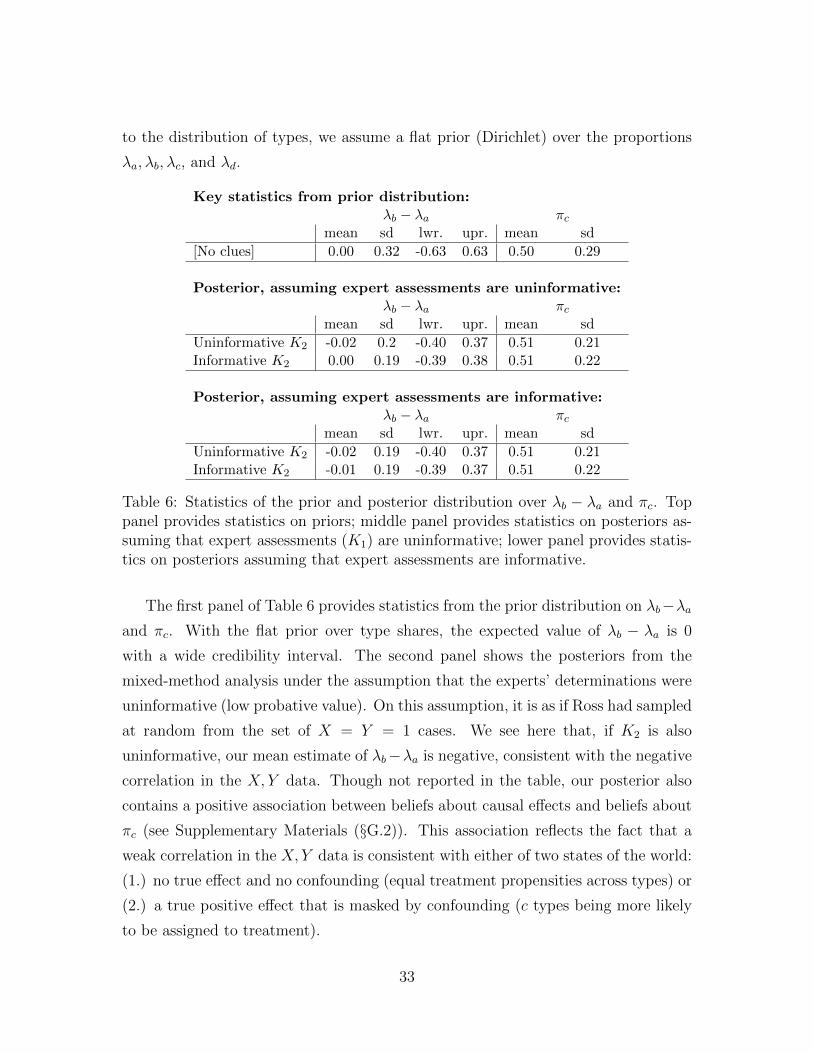
to the distribution of types, we assume a flat prior (Dirichlet) over the proportions

λa, λb, λc, and λd.

Key statistics from prior distribution:λb − λa πc

mean sd lwr. upr. mean sd

[No clues] 0.00 0.32 -0.63 0.63 0.50 0.29

Posterior, assuming expert assessments are uninformative:λb − λa πc

mean sd lwr. upr. mean sd

Uninformative K2 -0.02 0.2 -0.40 0.37 0.51 0.21Informative K2 0.00 0.19 -0.39 0.38 0.51 0.22

Posterior, assuming expert assessments are informative:λb − λa πc

mean sd lwr. upr. mean sd

Uninformative K2 -0.02 0.19 -0.40 0.37 0.51 0.21Informative K2 -0.01 0.19 -0.39 0.37 0.51 0.22

Table 6: Statistics of the prior and posterior distribution over λb − λa and πc. Toppanel provides statistics on priors; middle panel provides statistics on posteriors as-suming that expert assessments (K1) are uninformative; lower panel provides statis-tics on posteriors assuming that expert assessments are informative.

The first panel of Table 6 provides statistics from the prior distribution on λb−λaand πc. With the flat prior over type shares, the expected value of λb − λa is 0

with a wide credibility interval. The second panel shows the posteriors from the

mixed-method analysis under the assumption that the experts’ determinations were

uninformative (low probative value). On this assumption, it is as if Ross had sampled

at random from the set of X = Y = 1 cases. We see here that, if K2 is also

uninformative, our mean estimate of λb−λa is negative, consistent with the negative

correlation in the X, Y data. Though not reported in the table, our posterior also

contains a positive association between beliefs about causal effects and beliefs about

πc (see Supplementary Materials (§G.2)). This association reflects the fact that a

weak correlation in the X, Y data is consistent with either of two states of the world:

(1.) no true effect and no confounding (equal treatment propensities across types) or

(2.) a true positive effect that is masked by confounding (c types being more likely

to be assigned to treatment).

33

What happens if we treat the qualitative clues examined by Ross (K2) as highly

informative about effects in the individual cases? We see the result in the second

row of the second panel. Here our mean estimate of λb − λa hardly moves, rising to

approximately zero, with a very wide credibility interval. Likewise, the posterior on

πc increases just marginally.

In the third panel, we now assume that expert assessments—the clue used to

determine process-tracing sample selection—are highly informative. Our willingness

to make such an assumption would, of course, depend on our beliefs about how

such judgments were formed. Focusing on the second row, we see that, even if

assume both clues to be highly informative, the process-tracing yields virtually no

change in posterior means or uncertainty relative to the estimates derived from purely

correlational evidence.

This analysis illustrates some general features of the integration of qualitative

and quantitative causal inferences. First, it highlights some of the informational

demands that are required to perform formal inference from mixed data. Of partic-

ular importance here is the need to understand, and explicitly model, the criteria

used to select cases for process tracing from the quantitative sample. Second, the

analysis—especially in comparison to Application 1—highlights an important limit

to the capacity of small-n work to shape population-level inferences. Recall that Ross

finds causal-process evidence that natural resources were a driver of conflict in four

of five cases on which process tracing was carried out. This finding stands in appar-

ently sharp contrast to the X, Y pattern of a small negative correlation. However,

even when we take Ross’s clues to be highly probative—treating causal conclusions

about these five cases to be nearly certain—our posterior hardly shifts from the

correlational finding. The result suggests that, at least for estimating population-

level quantities, relative numbers matter: that in some circumstances even strong

process-tracing evidence, gathered on a small number of cases, will have only a very

modest impact on conclusions drawn from the quantitative analysis of a much larger

sample. We turn now to a more general examination of the consequences of mixing

quantitative and qualitative observations in differing proportions.

34

Implications for research design

We now illustrate the model’s usefulness in guiding research-design choices. Our focus

here is on characterizing the kind of learning that emerges from different combina-

tions of investment in the collection of correlational as compared with process-tracing

data under different research conditions. We report the results here of simulation-

based experiments designed to tell us under what research conditions different mixes

of methods can be expected to yield more accurate inferences. We also discuss, at

a high level, the implications of the framework for strategies of qualitative case-

selection.

As a metric of the returns from different research strategies we calculate the

expected inaccuracy in the estimation of the average treatment effect, as given in

equation 5.

L = Eθ(ED|θ(τ(θ)− τ̂(D))2) (5)

where τ(θ) is the value of λb−λa (the average treatment effect) given θ, and τ̂(D)

is the estimate of this treatment effect (the mean posterior value) that is generated

following some realization of data D. Thus, if some θ characterized the true state

of the world, then ED|θ(τ θ − τ̂)2 is the expected error in estimation of the causal

effect given different realizations of the data, D, that could obtain in this state of the

world. L is then the expected value of these errors given prior beliefs over possible

values of θ.

The general simulation procedure as follows. We first draw a set of “true” pa-

rameter values from a prior distribution. For priors on type proportions, we use a

Dirichlet distribution; for priors for each of the π and φ parameters, we use indepen-

dent Beta distributions.14 From each set of “true” parameter values, we then draw a

data realization for a particular research design—a particular number of correlational

and process-tracing cases—and then calculate the posterior on the average treatment

effect for that data realization. Then, by comparison with the “truth,” we calculate

the expected loss. We examine such estimates for a range of levels of investment in

qualitative and quantitative evidence. In most of the experiments, we also systemat-

ically vary the prior distribution for one parameter of the research situation between

14While by construction priors on each parameter are independent, this will not generally be thecase for posterior distributions.

35

two extreme positions, and observe the resulting change in the expected losses aris-

ing from different research designs. Further details of the simulation exercises can

be found in the Supplementary Materials (§H.5).

A few further features of the experiments are worth noting. First, our illustra-

tions focus on learning about population-level causal effects; however, the model can

yield results about the benefits of alternative research designs for estimating a wide

range of other quantities of interest, such as case-specific causal explanations or clue

probabilities. Second, while we focus on the search for a single clue in each case, the

analysis can be extended to the case of an arbitrarily large set of clues. Third, in

many of these experiments, the probative values are set at doubly decisive levels for

all φ parameters, and thus focus on the very optimistic case of maximally informa-

tive process tracing. Fourth, we illustrate tradeoffs at low levels of n, but the model

can be employed to inform choices for arbitrarily large numbers of cases. Finally, we

note that some results may be sensitive to the choice of priors. The results below

should thus be understood as an illustration of the utility of the BIQQ framework

for guiding research choices, rather than as a set of general prescriptive design rules.

Varieties of mixing

What are the marginal gains from additional pieces of correlational and process-

tracing evidence for the accuracy of causal estimates? Figure 3 displays the results,

plotting the errors associated with different mixes of correlational and process data.

Each dot represents a single possible research design, with the x-axis charting the

total the number of cases examined. For all cases, X and Y data are collected.

The shading of the dots in each column then represents the proportion of cases for

which process-tracing is also carried out. An unshaded dot is a design in which only

correlational data have been collected for all cases; a black dot is a design in which

the process-tracing clue is sought in all cases; and shades of grey, as they darken,

indicate process tracing for increasing shares of cases. For n ≤ 4 we report results for

all designs; for n > 4 we report only results when within case information is sought

for all, half, or none of the cases.

We see first from the graph that, as one would expect, moving from lower-n to

higher-n designs reduces the expected error of estimates. Further, both adding a

36

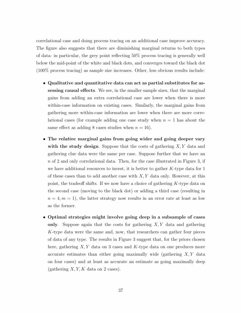
correlational case and doing process tracing on an additional case improve accuracy.

The figure also suggests that there are diminishing marginal returns to both types

of data: in particular, the grey point reflecting 50% process tracing is generally well

below the mid-point of the white and black dots, and converges toward the black dot

(100% process tracing) as sample size increases. Other, less obvious results include:

• Qualitative and quantitative data can act as partial substitutes for as-

sessing causal effects. We see, in the smaller sample sizes, that the marginal

gains from adding an extra correlational case are lower when there is more

within-case information on existing cases. Similarly, the marginal gains from

gathering more within-case information are lower when there are more corre-

lational cases (for example adding one case study when n = 1 has about the

same effect as adding 8 cases studies when n = 16).

• The relative marginal gains from going wider and going deeper vary

with the study design. Suppose that the costs of gathering X, Y data and

gathering clue data were the same per case. Suppose further that we have an

n of 2 and only correlational data. Then, for the case illustrated in Figure 3, if

we have additional resources to invest, it is better to gather K-type data for 1

of these cases than to add another case with X, Y data only. However, at this

point, the tradeoff shifts. If we now have a choice of gathering K-type data on

the second case (moving to the black dot) or adding a third case (resulting in

n = 4,m = 1), the latter strategy now results in an error rate at least as low

as the former.

• Optimal strategies might involve going deep in a subsample of cases

only. Suppose again that the costs for gathering X, Y data and gathering

K-type data were the same and, now, that researchers can gather four pieces

of data of any type. The results in Figure 3 suggest that, for the priors chosen

here, gathering X, Y data on 3 cases and K-type data on one produces more

accurate estimates than either going maximally wide (gathering X, Y data

on four cases) and at least as accurate an estimate as going maximally deep

(gathering X, Y,K data on 2 cases).

37

●

●

●

●

●

●

●

●

Number of Cases

Exp

ecte

d E

rror

●

●

●

●

●

●

●

●

●

●

●

●

●

●●

●

●

●

●

●

●

1 2 3 4 8 16 32 64 128

0.00

0.02

0.04

0.06

0.08

Figure 3: Expected errors in the estimation of average treatment effects for designsin which X, Y , data are sought in n studies (horizontal axis) and clue data aresought within m of these. The shading of dots indicates the proportion of cases forwhich within-case data are sought (white = none; black = all). For small samplesizes (n ∈ {1, 2, 3, 4}) we show results for all designs (m ∈ {1, 2, . . . , n}). For largersample sizes, we show only designs with clues sought in 0, half, and all cases.

Designs in Context

More generally, the optimal level of mixing ought to depend on context—on features

of the research situation that affect the problem, and the available tools, of infer-

ence. In the next subsections, we report results from experiments in which we vary

the researcher’s priors about (a.) the probative value of clues, (b.) heterogeneity of

treatment effects (c.) uncertainty regarding assignment processes, and (d.) uncer-

tainty regarding the probative value of clues. In all cases we report the expected loss

for the design in question, as given in Equation 5.

38

Probative value of clues

If clues have no probative value — in the sense that priors over φjx do not depend

on type, j — then gathering data on clues does not affect inference. Probative value

does not get picked up during analysis, it must be imported. Less clear, however, is

the extent to which gains in inference depend on the degree of probative value (see

footnote 5). Our simulation evidence from full BIQQ estimation (Figure 4) suggests

that, in some ranges at least, the gains are also convex — that is, increasingly more

is learned as the gaps between pairs such as φb1 and φd1 increases. The top left panel

of Figure 4 shows an example of these convex gains, showing expected losses for the

setting in which there is no probative value, the setting in which all tests are doubly

decisive, and the situation halfway between these extremes.

Effect Heterogeneity

We might expect that the optimal research design for estimating average treatment

effects would depend on how heterogeneous the true causal effects are in the popula-

tion. If we believe that effects are strongly homogeneous, then confidence that one

case is affected by treatment provides a great deal of information about population

treatment effects. However, if effects are believed to be highly heterogeneous, then

knowing that one case is affected by treatment provides less information regarding

effects on other cases.

Heterogeneity can be conceptualized in different ways. Here, however, we define

heterogeneity as increasing in the amount of variance in causal effects across cases

in the population. In the binary environment, for any τ ∈ [0, 1], maximum effect

heterogeneity is obtained when λa = (1−τ)/2 and λb = (1+τ)/2: i.e., when all cases

have either a positive or negative treatment effect, with no destined or chronic cases.

For a positive treatment effect, maximum homogeneity occurs when a = 0, b = τ ,

with the remaining share 1 − τ consisting of types c and d. For negative treatment

effects, homogeneity is maximized with λb = 0. For an average treatment effect of 0,

there are two possibilities: no treatment effect for any case (maximal homogeneity),

or a positive effect for half the cases and a negative effect for the other half (maximal

heterogeneity).

Using this conceptualization of heterogeneity, our simulation results confirm that

39

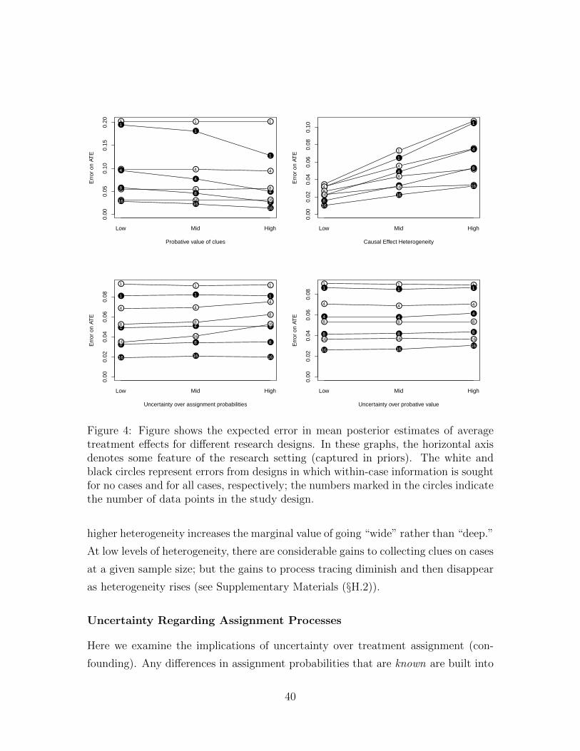
Probative value of clues

Err

or o

n AT

E

● ● ●1 1 1●

●

●

11

1

● ● ●4 4 4●

●

●

4

4

4● ● ●8 8 8●●

●

88

8● ● ●16 16 16● ●●

1616

16

Low Mid High

0.00

0.05

0.10

0.15

0.20

Causal Effect Heterogeneity

Err

or o

n AT

E

●

●

●

1

1

1

●

●

●

1

1

1

●

●

●

4

4

4

●

●

●

4

4

4

●

●●

8

8

8

●

●

●

8

8

8

●● ●

16

16 16

●

●

●

16

16

16

Low Mid High

0.00

0.02

0.04

0.06

0.08

0.10

Uncertainty over assignment probabilities

Err

or o

n AT

E

● ● ●1 1 1

● ● ●1 1 1

● ●●

4 44

● ● ●4 4 4● ●●

8 8

8

● ● ●8 8 8●●

●

1616

16

● ● ●16 16 16

Low Mid High

0.00

0.02

0.04

0.06

0.08

Uncertainty over probative value

Err

or o

n AT

E

● ● ●1 1 1● ● ●1 1 1

● ● ●4 4 4

● ●●4 44

● ● ●8 8 8

● ● ●8 8 8

● ● ●16 16 16

● ● ●16 16

16

Low Mid High

0.00

0.02

0.04

0.06

0.08

Figure 4: Figure shows the expected error in mean posterior estimates of averagetreatment effects for different research designs. In these graphs, the horizontal axisdenotes some feature of the research setting (captured in priors). The white andblack circles represent errors from designs in which within-case information is soughtfor no cases and for all cases, respectively; the numbers marked in the circles indicatethe number of data points in the study design.

higher heterogeneity increases the marginal value of going “wide” rather than “deep.”

At low levels of heterogeneity, there are considerable gains to collecting clues on cases

at a given sample size; but the gains to process tracing diminish and then disappear

as heterogeneity rises (see Supplementary Materials (§H.2)).

Uncertainty Regarding Assignment Processes

Here we examine the implications of uncertainty over treatment assignment (con-

founding). Any differences in assignment probabilities that are known are built into

40

our priors in a Bayesian setting and do not produce biases (just as known confounds

can be controlled for in a standard regression model). However, uncertainty about as-

signment processes still generates higher variance in posterior estimates (see Gerber,

Green, and Kaplan, 2004).

In the BIQQ framework, clues provide discriminatory leverage on case types that

is independent of assignment probabilities: with strong probative value, b- and d-type

treated units can be distinguished, thus eliminating the identification problem gener-

ated by uncertain assignment propensities. In our simulations (bottom left panel of

Figure 4), we find that greater uncertainty over assignment processes indeed results

in greater errors for correlational analysis — most clearly, at higher n. However,

for the parameter space we examine, and assuming strongly probative clues, uncer-

tainty about assignment does not reduce accuracy for mixed-method analysis. (See

Supplementary Materials (§H.3).)

Uncertainty regarding the probative value of clues

As with assignment probabilities, researchers may be uncertain regarding the proba-

tive value of clues for discriminating between types. How much does this uncertainty

matter for the relative gains to qualitative evidence?

Our experiment fixes the expected probative value of a clue and allows for variance

around that expected value. Informally, we are thus comparing a situation in which

one believes that a clue has moderate probative value to one in which one believes

that it may have strong probative value or it may have none at all. Surprisingly, our

simulations suggest that for very low n, uncertainty over the probative values of clues

is relatively unimportant for expected errors (see Supplementary Materials (§H.4)).

And, while we observe penalties to uncertainty, there is learning from within-case

information even with very high levels of uncertainty.

To be clear, this analysis does not imply that there is no penalty to being wrong

about the probative value of clues. The result suggests rather, that having more,

rather than less, uncertainty about that probative value may sometimes be relatively

inconsequential for the choice of research strategy, at least with a low n.

41

Case Selection

A critical decision for scholars employing mixed methods is to determine which cases

are most valuable for within-case analysis.

In our framework the answer depends in large part on the configuration of φjx

values. For the basic insight, consider a situation in which, for a given clue, we have

φb1=0.5; φd1=0.5; φb0=0.5; and φc0=0.1 (taking these to be known). In this situation,

searching for the clue in X = Y = 1 cases will yield no leverage since the clue does

not discriminate between the two types (b and d) that need to be distinguished given

X = Y = 1. Here there is no additional learning about λb that can be gained from

looking for the clue. In contrast, X = 0, Y = 0 cases will be informative because

the clue is much better at distinguishing between untreated b and c types—the two

types in contention for this kind of case. Thus, for estimating λb and for these clue

probabilities, process tracing an X = Y = 0 case will be productive, while process-

tracing an X = Y = 1 case will not.

While it is common practice for mixed-method researchers to perform their pro-

cess tracing “on the regression line,” the BIQQ framework suggests that the gains to

process tracing for different X and Y values in fact depend on the particular constel-

lations of φ values for the potentially available clues. More generally, the framework

allows one to assess the expected gains from any given case-selection strategy ex ante

once priors have been specified.

Conclusion

Despite broad agreement that mixing methods is a good idea, scholars have produced

limited guidance about how to integrate information gathered from qualitative and

quantitative approaches. As we have shown, because the inferential strategies of both

qualitative and quantitative analyses can be described in Bayesian terms, it is a short

step to combine the two forms of inference within a single analytic framework. More

broadly, the approach can be seen as a simple application of the general structure

of Bayesian networks, as advocated for example by Pearl (2000) and others, to the

problem of combining inferences from qualitative and quantitative data. Though

conceptually simple, however, no integrated Bayesian approach like BIQQ has, to

42

our knowledge, been developed or used for this purpose.

While the BIQQ model does not seek to bridge all aspects of the qualitative-

quantitative divide, it does achieve integration on four important fronts. First, it

provides a method for combining the leverage derived from correlational and process-

based data to arrive at a single set of causal inferences. Second, the framework

uses the leverage derived from one form of data to inform the premises underlying

the interpretation of the other form of data. In doing so, it thus demonstrates

a precise sense in which mixing methods can sometimes be better than maximal

investment in a single method. Third, while we have not emphasized the point here,

the framework can be used not just to estimate average causal effects but also to

address questions more commonly associated with small-n research (did X cause

Y in this case? what is the mechanism of causation?). Notably, the framework

moves beyond the standard quantitative solution to the fundamental problem of

causal inference—i.e., estimating average effects for a population. BIQQ’s typological

framework, in an important sense, keeps the inferential focus on potential outcomes

at the level of the case, allowing us to building estimates of average treatment effects

from case-level explanations and estimates of the distribution of causal effects in

the population. Finally, we have shown how the approach can provide guidance on

mixed-method research designs to researchers allocating resources at the margins.

We close by considering the demands that the BIQQ framework imposes on the

researcher and the research process. The critical demand is that researchers be able

to state a prior distribution over three distinct sets of quantities: the causal effects

being assessed, the assignment process, and clue probabilities by type and treatment

condition. This is, in a certain sense, a very tall order. In present work, scholars

using process tracing sometimes indicate what kind of evidence they expect to find

if a relationship is causal; but rarely do scholars indicate probabilities for these

observations for different possible causal effects or specify the uncertainty they hold

over these probabilities. The BIQQ framework thus requires greater explicitness and

completeness in the specification of the assumptions underlying analysis.

What if the researcher does not have specific, well-developed priors on the primi-

tives entering into the analysis? As we have noted, learning in the BIQQ framework

can occur even with “flat” priors over causal effects and assignment probabilities.

And in some settings, such as in experimental work, assignment probabilities may be

43

known with certainty. The greatest challenge we see is in the specification of priors

over the probative value of clues. How is one to know, even approximately, the likeli-

hood of observing a given clue conditional upon a causal type (itself a metaphysical

concept) and treatment status?15

One response is to abandon the project of formally drawing inferences from clues.

Even at an informal level, we believe that the principles underlying the BIQQ ap-

proach can offer heuristic guidance in the interpretation of mixes of qualitative and

quantitative evidence. We see, however, three more constructive approaches to the

problem of specifying priors over the probative value of qualitative evidence.

The first is to emphasize the conditional nature of inference, with conclusions

reported as conditional on a clearly specified set of priors. For example, if clue

probabilities are provided by theory, then posteriors are theory-conditional claims.

If a theory T suggests that clue K will be observed if and only if X causes Y ,

then the presence of K provides evidence that X causes Y only to the extent that T

provides a true account of the causal relationship between X and Y . If T captures

the wrong mechanism of causation, for instance, then clue probabilities that derive

from the theory may be wrong and causal inferences that draw on these may be

wrong. Under such an approach it would be natural to show the sensitivity of results

to varying conditions, as we have illustrated in the analysis of the causes of civil war.

A second approach is to adopt a subjective Bayes perspective and seek to elicit

what is actually believed prior to analysis. Given a set of subjective prior beliefs, the

model can tell us what we ought to believe as a matter of consistency after observing

the data. These subjective beliefs may be informed by, even if they cannot be formally

derived from, arguments from theory and existing evidence. A subjective Bayes

approach also faces a number of challenges. One is that researchers’ and readers’

priors may vary. In response, scholars might seek to ground priors on some systematic

measure of collective beliefs, drawn for instance from a survey of existing findings or

of experts in the relevant field (Gill and Walker, 2005).16 A second concern is that the

15Note that in this discussion we treat beliefs over the probative value of clues as part of theresearcher’s priors. The same substantive issues arise even if, technically, there is no specification ofpriors over the φ parameters, or over any parameters, as these will nevertheless enter the likelihood.(For an example using a maximum likelihood approach, see Supplementary Material J.) In an MLEcontext, the focus simply turns to a need to defend a model rather than a set of priors.

16On the challenges of eliciting experts’ priors faithfully and carefully, and potential responses tothese problems, see Schlag, Tremewan, and Van der Weele (2013).

44

formulation of numerical priors may be difficult. While we suspect that this will strike

some readers as a significant obstacle to the framework’s implementation, we believe

that the difficulties can be overstated. Ordinary language terms such as “more likely”

or “less likely” necessarily imply ordinal restrictions on quantitative relations that

can be used to structure priors. It might be more difficult to translate notions such

as “much more likely” or “much less likely” into cardinal differences in probabilities.

Yet most qualitative beliefs, if they have substantive content, minimally imply an

upper or lower bound on the probability differentials involved.17 Uncertainty about

probabilities can also be readily expressed in the framework, and results probed for

sensitivity to alternative specifications of that uncertainty.

Of course, subjective priors, even if accurately and precisely elicited, may still be

incorrect and lead to false conclusions. We believe that it is thus worth exploring

a third approach, grounded in objective Bayes. In an objective Bayes’ setting, we

would begin with uninformative priors—such as priors that maximize entropy (see

for example Williamson (2004))—and let the data do all the work. In certain em-

pirical situations, it may be possible to begin with uninformative priors about clue

probabilities, and then to use a mix of qualitative and quantitative data to update

beliefs about probative value, while simultaneously using the clue observations to

inform causal inferences (see Supplementary Materials (§I) for elaboration on this

point). A critical avenue for future research, in our view, is the specification of the

empirical conditions under which process tracing can yield inferential leverage in the

absence of assumptions about probative value.

The demands of both the subjective and objective Bayes approaches are consid-

erable. We believe, however, that the model is useful in part because it places such

high demands on scholars’ beliefs: i.e., because it clearly identifies the required in-

puts into the process of drawing integrated causal inferences. Put differently, to the

extent that scholars are unable to specify even approximate ranges on the relevant

parameters, this is a problem for causal inference, not for the BIQQ framework. The

framework helps identify the kinds of knowledge we need to generate if we are to

make better use of mixed methods to provide causal accounts of the world.

17For instance, a scholar who believes that a clue is “much more” likely if a causal effect has oc-curred than if it hasn’t should be able at least to exclude some numerical differences as insufficientlylarge to count as “much more.”

45

Supplementary Materials

In the paper’s online Supplementary Materials, we provide additional details on

the approach developed here as well as further information on the applications and

simulations.

§A : Probabilistic logics in existing work using process tracing

§B : Bayesian process tracing: intuition and illustration

§C : Bayesian correlational inference: intuition and illustration

§D : BIQQ Inference Step by Step

§E : Code to Implement baseline BIQQ model using Stan

§F : Extensions

§G : Notes on Applications

§H : Notes on Simulations

§I : Learning from non-discriminating clues

§J : Maximum Likelihood Integration

46

References

Barton, Allen H., and Paul F. Lazarsfeld. 1955. Some functions of qualitative analysis

in social research. Vol. 181 Bobbs Merrill.

Beach, Derek, and Rasmus Brun Pedersen. 2013. Process-Tracing Methods: Founda-

tions and Guidelines. University of Michigan Press.

Beck, Nathaniel. 2010. “Causal Process ‘Observation’: Oxymoron or (Fine) Old

Wine.” Political Analysis 18 (4): 499–505.

Bennett, Andrew. 2008. “Process Tracing. A Bayesian Perspective.” In The Ox-

ford Handbook of Political Methodology, ed. Janet M. Box-Steffensmeier, Henry E.

Brady, and David Collier. Oxford, UK: Oxford University Press.

Bennett, Andrew. 2010. “Process tracing and causal inference.” In Rethinking social

inquiry: Diverse tools, shared standards, ed. David Collier and Henry E Brady.

Lanham, MD: Rowman & Littlefield.

Bennett, Andrew. 2015. “Appendix.” In Process Tracing: From Metaphor to Analytic

Tool, ed. Andrew Bennett and Jeffrey Checkel. New York: Cambridge University

Press.

Boix, Carles. 1999. “Setting the Rules of the Game: The Choice of Electoral Systems

in Advanced Democracies.” The American Political Science Review 93 (3): pp.

609-624.

Brady, H.E., and D. Collier. 2004. Rethinking Social Inquiriy: Diverse Tools, Shared

Standards. Lanham, MD: Rowman & Littlefield.

Chickering, David Maxwell, and Judea Pearl. 1996. “A clinician’s tool for analyzing

non-compliance.” In Proceedings of the National Conference on Artificial Intelli-

gence. pp. 1269–1276.

Collier, David. 2011. “Understanding proces tracing.” PS: Political Science and Pol-

itics 44 (04): 823–30.

47

Collier, David, Henry E Brady, and Jason Seawright. 2004. “Sources of leverage

in causal inference: Toward an alternative view of methodology.” In Rethinking

social inquiry: Diverse tools, shared standards, ed. David Collier and Henry E

Brady. Lanham, MD: Rowman & Littlefield.

Collier, David, Henry E Brady, and Jason Seawright. 2010. “Sources of leverage

in causal inference: Toward an alternative view of methodology.” In Rethinking

social inquiry: Diverse tools, shared standards, ed. David Collier and Henry E

Brady. Lanham, MD: Rowman & Littlefield.

Collier, P., and N. Sambanis. 2005. Understanding Civil War: Africa. Stand Alone

Series World Bank.

Collier, Paul, and Anke Hoeffler. 2004. “Greed and grievance in civil war.” Oxford

economic papers 56 (4): 563–595.

Creswell, J.W., and Amanda L. Garrett. 2008. “The ”movement” of mixed meth-

ods research and the role of educators.” South African Journal of Education 28

(08/2008): 321 - 333.

Ericson, William A. 1969. “Subjective Bayesian models in sampling finite popula-

tions.” Journal of the Royal Statistical Society. Series B (Methodological): 195–233.

Fairfield, Tasha. 2013. “Going Where the Money Is: Strategies for Taxing Economic

Elites in Unequal Democracies.” World Development 47 (0): 42 - 57.

Freedman, David A. 2010. “On Types of Scientific Inquiry: The Role of Qualita-

tive Reasoning.” In Rethinking social inquiry: Diverse tools, shared standards, ed.

David Collier and Henry E Brady. Lanham, MD: Rowman & Littlefield.

Gelman, Andrew, John B Carlin, Hal S Stern, David B Dunson, Aki Vehtari, and

Donald B Rubin. 2013. Bayesian Data Analysis. Boca Raton, FL: CRC Press.

Gerber, Alan S., Donald P. Green, and Edward H. Kaplan. 2004. “The illusion of

learning from observational research.” In Problems and Methods in the Study of

Politics, ed. Ian Shapiro, Rogers M. Smith, and Tarek E. Masoud. Cambridge,

UK: Cambridge University Press.

48

Gerring, J. 2012. Social Science Methodology: A Unified Framework. Strategies for

Social Inquiry Cambridge University Press.

Gill, Jeff, and Lee D. Walker. 2005. “Elicited Priors for Bayesian Model Specifications

in Political Science Research.” Journal of Politics 67 (3): 841–872.

Glynn, Adam N, Jon Wakefield, Mark S Handcock, and Thomas S Richardson.

2008. “Alleviating linear ecological bias and optimal design with subsample data.”

Journal of the Royal Statistical Society: Series A (Statistics in Society) 171 (1):

179–202.

Glynn, Adam N., and Kevin M. Quinn. 2011. “Why Process Matters for Causal

Inference.” Political Analysis 19: 273-286.

Glynn, Adam N., and Nahomi Ichino. 2014. “Using Qualitative Information to Im-

prove Causal Inference.” American Journal of Political Science: n/a–n/a.

Goertz, G., and J. Mahoney. 2012. Tale of Two Cultures - Contrasting Qualitative

and Quantitative. University Press Group Limited.

Gordon, Sanford C, and Alastair Smith. 2004. “Quantitative leverage through quali-

tative knowledge: Augmenting the statistical analysis of complex causes.” Political

Analysis 12 (3): 233–255.

Hall, Peter A. 2003. “Aligning Ontology and Methodology in Comparative Research.”

In Comparative Historical Analysis in the Social Sciences, ed. James Mahoney and

Dietrich Rueschemeyer. Cambridge, UK and New York: Cambridge University

Press.

Herron, Michael, and Kevin Quinn. 2009. “A Careful Look at Modern Case Selection

Methods.” Paper Presented at the 67th Annual Meeting of the Midwest Political

Science Association.

Imbens, Guido W, and Donald B Rubin. 1997. “Bayesian inference for causal effects

in randomized experiments with noncompliance.” The Annals of Statistics: 305–

327.

49

King, G., R.O. Keohane, and S. Verba. 1994. Designing Social Inquiry: Scientific

Inference in Qualitative Research. Princeton University Press.

Kreuzer, Marcus. 2010. “Historical Knowledge and Quantitative Analysis: The Case

of the Origins of Proportional Representation.” American Political Science Review

104 (5): 369–392.

Lengfelder, Christina. 2012. “Triangular Development Cooperation: How emerging

powers change the landscape of development cooperation.” Phd dissertation Uni-

versidad Catolica de Chile.

Lieberman, E.S. 2003. Race and Regionalism in the Politics of Taxation in Brazil and

South Africa. Cambridge Studies in Comparative Politics Cambridge University

Press.

Lieberman, Evan S. 2005. “Nested Analysis as a Mixed-Method Strategy for Com-

parative Research.” American Political Science Review 99 (7): 435–452.

Mahoney, James. 2012. “The Logic of Process Tracing Tests in the Social Sciences.”

Sociological Methods and Research 41 (4): 570-597.

Paluck, Elizabeth Levy. 2010. “The Promising Integration of Qualitative Methods

and Field Experiments.” The ANNALS of the American Academy of Political and

Social Science 628 (1): 59-71.

Pearl, Judea. 2000. Causality: models, reasoning and inference. Vol. 29 Cambridge

Univ Press.

Rohlfing, Ingo. 2012. Case Studies and Causal Inference: An Integrative Framework.

Research Methods Series New York: Palgrave Macmillan.

Ross, Michael L. 2004. “How do natural resources influence civil war? Evidence from

thirteen cases.” International organization 58 (01): 35–67.

Rubin, Donald B. 1974. “Estimating Causal Effects of Treatments in Randomized

and Nonrandomized Studies.” Journal of Educational Psychology 66: 688–701.

50

Schlag, Karl H, James Tremewan, and Joel J Van der Weele. 2013. “A penny for your

thoughts: a survey of methods for eliciting beliefs.” Experimental Economics: 1–

34.

Seawright, Jason. ND. Multi-method social science: Combining qualitative and quan-

titative tools. Cambridge University Press.

Seawright, Jason, and John Gerring. 2008. “Case Selection Techniques in Case Study

Research: A Menu of Qualitative and Quantitative Options.” Political Research

Quarterly 61 (2): 294-308.

Stan Development Team. 2014. “RStan: the R interface to Stan, Version 2.5.0.”

http://mc-stan.org/rstan.html.

Stokes, S.C. 2001. Mandates and Democracy: Neoliberalism by Surprise in Latin

America. Cambridge Studies in Comparative Politics Cambridge University Press.

Swank, D. 2002. Global Capital, Political Institutions, and Policy Change in De-

veloped Welfare States. Cambridge Studies in Comparative Politics Cambridge

University Press.

Van Evera, Stephen. 1997. Guide to methods for students of political science. Ithaca,

NY: Cornell University Press.

Western, Bruce, and Simon Jackman. 1994. “Bayesian Inference for Comparative

Research.” American Political Science Review 88 (6): 412–423.

White, Howard, and Daniel Philips. 2012. Addressing attribution of cause and ef-

fect in small n impact evaluations: towards an integrated framework. Techni-

cal Report 15 International Initiative for Impact Evaluation Working Papers.

http://www.3ieimpact.org/media/filer/2012/06/29/working paper 15.pdf.

Williamson, Jon. 2004. “Bayesian nets and causality: philosophical and computa-

tional foundations.”.

Young, Forrest W. 1981. “Quantitative analysis of qualitative data.” Psychometrika

46 (4): 357–388.

51

Zaks, Sherry. 2013. “Relationships Among Rivals: Contending Hypotheses and the

Logic of Process Tracing.” Paper prepared for the Short Course 1 on Multi-Method

Research, 2012 Annual Meeting of the American Political Science Association:

New Orleans, Louisiana.

52

Supplementary Materials for

Macartan Humphreys and Alan M. Jacobs,

“Mixing Methods: A Bayesian Approach,”

American Political Science Review

§A : Probabilistic logics in existing work using process tracing

§B : Bayesian process tracing: intuition and illustration

§C : Bayesian correlational inference: intuition and illustration

§D : BIQQ Inference Step by Step

§E : Code to Implement baseline BIQQ model using Stan

§F : Extensions

§G : Notes on Applications

§H : Notes on Simulations

§I : Learning from non-discriminating clues

§J : Maximum Likelihood Integration

53

A Probabilistic logics in existing work using

process tracing

The Bayesian formalization of process tracing developed in the paper builds on

an empirical logic that is already common in current accounts and, to a lesser

extent, applications of process tracing.

Van Evera’s hoop, smoking gun, and doubly decisive tests have played a central

role in accounts of the logic of process tracing. Consistent with the logic of

process tracing embedded in the BIQQ framework, these tests involve reasoning

about the likelihood of observing particular pieces of evidence under alternative

hypotheses. A notable feature of early accounts is that they described process

tracing tests as grounded in an empirical logic of necessity and sufficiency. In

a hoop test for a hypothesis, H, for instance, the observation of a given piece

of evidence, K, was characterized as being necessary for the survival of H

(though not sufficient for its affirmation). This corresponds in our framework

to Pr(K = 1|H) = 1. Likewise, in a smoking gun test, the observation of a piece

of evidence, K, was characterized as being sufficient for the confirmation of H

(though not necessary for its survival), formally Pr(K = 1|¬H) = 0 (Collier,

2011, 825-827; Mahoney, 2012, 5 and 7; Bennett, 2010, 210). Thus, some

test outcomes—the passage of a smoking gun test, the failure of a hoop test,

and either outcome in a double decisive test—were seen as having categorical

(pass/fail) consequences for the hypothesis.

These early accounts thus suggested a deterministic feature of process tracing

tests different from that taken in this paper.

Even in these accounts, however, the relationship between hypotheses and ev-

idence was at least implicitly understood as partially uncertain; and some test

outcomes were understood as incrementally shifting beliefs in a manner more

consistent with Bayesian reasoning. The passage of a hoop test or the fail-

ure of a smoking gun test were seen as somewhat strengthening and weaken-

ing a hypothesis, respectively. They thus implicitly reflected probabilities for

Pr(K = 1|¬H), for the hoop test, and Pr(K = 1|H), for the smoking gun test,

that lay between 0 and 1 (exclusive). Mahoney (2012) also points out that

54

hoop tests and smoking gun tests may be more or less difficult, depending on

the commonness of the evidence (pp. 7 and 9). This consideration corresponds

directly to the denominator in Bayes’ rule.

Further, “straw in the wind” tests—where, in effect, Pr(K = 1|H) 6= Pr(K =

1|¬H) both lie strictly between 0 and 1—were seen as shifting beliefs somewhat

toward or against the hypothesis, though treated as modest sources of inferen-

tial leverage. Indeed, Zaks (2013) points to the central importance of “pieces

of evidence that are not quite definitive enough to qualify as either sufficient

or necessary”, but that nonetheless “may lend support to (or undermine) an

explanation” (p. 11). Zaks relabels these as “leveraging tests” to highlight the

key probative role that evidence with uncertain implications typically plays in

process tracing.

Collier (2011, p. 827), moreover, addresses the possibility of ambiguity about

the test type to which a causal process observation (CPO) corresponds, arising

from different background theories of or reasoning about the data-generating

process giving rise to the CPOs. Importantly, the BIQQ framework can capture

this kind of uncertainty not just by allowing the φ parameters to take on

intermediate values but also by allowing probability distributions over many

possible values.

We note that the focus of these accounts is, in effect, on the likelihood of

observing within-case data given different underlying processes. This focus

does not imply the use of a fully Bayesian approach. And, as we demonstrate

elsewhere in the Supplementary Materials (§J), a similar type of analysis to

that we propose can be undertaken using a maximum likelihood framework.

The Bayesian approach, however, better captures the accounts in this work of

how inferences are drawn from clue information (in terms of lending support

for one or another explanation) and, as noted above, the Bayesian approach

provides an intuitive way of handling uncertainty over probative value.

While largely compatible with these accounts, the approach taken in the BIQQ

framework is closest to that presented in recent accounts that embrace a fully

probabilistic view of process tracing. Bennett (2015), Beach and Pedersen

(2013, pp. 83ff), and Rohlfing (2012, p. 187–198) shift from the language of

55

sufficiency and necessity to a wholly probabilistic understanding of the re-

lationship between hypotheses and pieces of evidence. Beach and Pedersen

(2013, pp. 102), for instance, construe Van Evera’s concepts of “certainty”

and “uniqueness” as continua, representing differing probabilities of making a

given observation under a hypothesis. These accounts, moreover, formalize the

inferential reasoning involved in process tracing in Bayesian terms — as a func-

tion of the probability of the evidence, given the hypothesis; the unconditional

probability of the evidence; and the prior probability of the hypothesis.18 To

our knowledge, current approaches do not allow for uncertainty over probative

value (as opposed to intermediate probative value) or for joint uncertainty over

causal types, probative value, and assignment processes.

To date, surprisingly few substantive works using process tracing feature ex-

plicit reasoning about the test types to which the search for particular pieces

of evidence correspond or about the likelihood of observing pieces of evidence

under alternative hypotheses. Two rare exceptions are Lengfelder (2012) and

Fairfield (2013), which explicitly analyze CPOs in relation to Van Evera’s test

types. Fairfield (2013)’s treatment, moreover, treats inference from CPOs in an

explicitly probabilistic fashion. Reasoning about “how surprising the evidence

would be if a hypothesis were correct,” Fairfield distinguishes among hoop and

smoking gun tests according to their strength and the degree to which they

“increase or decrease the likelihood that a hypothesis is correct to varying de-

grees” (p. 55). So far, at least, clear probabilistic reasoning about qualitative

evidence has yet make the leap from principles to common practice.

18Critically, a probabilistic understanding of process tracing does not imply a probabilistic un-derstanding of causal relations. A Bayesian approach to inference is fully compatible, for instance,with a set-theoretic, deterministic approach to causation. Indeed, the potential outcomes frameworkunderlying the BIQQ approach itself assumes deterministic outcomes conditional on treatment.

56

B Bayesian process tracing: intuition and il-

lustration

B.1 The role of priors in Bayesian updating

We note in the text of the paper that the amount of learning that results from

a given piece of new data depends on prior beliefs.

Figure 5 illustrates these points. In each subgraph, we show how much learning

occurs under different scenarios. The horizontal axis indicates the level of prior

confidence in the hypothesis and the curve indicates the posterior belief that

arises if we do (or do not) observe the clue. As can be seen, the amount

of learning that occurs—the shift in beliefs from prior to posterior—depends

a good deal on what prior we start out with. For a smoking gun test, the

amount of learning is highest for values roughly in the 0.2 to 0.4 range—and

then declines as we have more and more prior confidence in our hypothesis. For

a hoop test, the amount of learning when the clue is not observed is greatest

for hypotheses in which we have middling-high confidence (around 0.6 to 0.8),

and minimal for hypotheses in which we have a very high or a very low level

of confidence.

The implication here is that our inferences with respect to a hypothesis must

be based not just on the search for a clue predicted by the hypothesis but also

on the plausibility of the hypothesis, based on other things we know. Suppose,

for instance, that we fail to observe evidence that we are 90 percent sure we

should observe if a hypothesized causal effect has occurred: a strong hoop test is

failed. But suppose that the existing literature has given us a very high level of

confidence that the hypothesis is right. This high prior confidence, sometimes

referred to as a “base rate,” is equivalent to believing that the causal effect

exists in a very high proportion of cases. Thus, while any given case with a

causal effect has only a 0.1 chance of not generating the clue, the high base

rate means that the vast majority of cases that we observe without the clue

will nonetheless be cases with causal effects. Thus, the failure of even a strong

hoop test, involving a highly certain prediction, should only marginally reduce

57

0.0 0.2 0.4 0.6 0.8 1.0

0.0

0.2

0.4

0.6

0.8

1.0

Straw in the Wind

φ0 = 0.4 , φ1 = 0.6 (PV = 0.2 )

prior

Pos

terio

r

p os ter io

r i f

c lue p re

sen t

pos ter io

r i f

c l ue

a bsen t

p

ri

o

r

0.0 0.2 0.4 0.6 0.8 1.0

0.0

0.2

0.4

0.6

0.8

1.0

Hoop

φ0 = 0.6 , φ1 = 0.95 (PV = 0.5 )

prior

Pos

terio

r

p os t er io

r i f

c lue p resen t

poster ior i f c lue absen t

pr

io

r

0.0 0.2 0.4 0.6 0.8 1.0

0.0

0.2

0.4

0.6

0.8

1.0

Smoking Gun

φ0 = 0.05 , φ1 = 0.4 (PV = 0.5 )

prior

Pos

terio

r

pos ter ior i f c lue present

pos ter io

r i f

c l u

e a bs

en t

p

ri

o

r

0.0 0.2 0.4 0.6 0.8 1.0

0.0

0.2

0.4

0.6

0.8

1.0

Doubly Decisive

φ0 = 0.05 , φ1 = 0.95 (PV = 0.9 )

prior

Pos

terio

r poster ior i f clue present

poster ior i f c lue absent

p

ri

o

r

Figure 5: Figure shows how the learning from different types of tests depends on priorsregarding the proposition. A “smoking gun” test has the greatest impact on beliefs whenpriors are middling low and the clue is observed; a “hoop test” has the greatest effect whenpriors are middling high and the clue is not observed. Here “PV” denotes the probativevalue of the test.

our confidence in a hypothesis that we strongly expect to be true.

A similar line of reasoning applies to smoking-gun tests involving hypotheses

that prior evidence suggests are very unlikely to be true. Innocent people may

be very unlikely to be seen holding smoking guns after a murder. But if a

very high proportion of people observed are known to be innocent, then a very

high proportion of those holding smoking guns will in fact be innocent—and a

smoking-gun clue will be far from decisive.

We emphasize two respects in which these implications depart from common

intuitions. First, we cannot make general statements about how decisive dif-

58

ferent categories of test, in Van Evera’s framework, will be. It is commonly

stated that hoop tests are devastating to a theory when they are failed, while

smoking gun tests provide powerful evidence in favor of a hypothesis. But, in

fact the degree of belief change depends not just on features of the clues but

also on prior beliefs.

Second, although scholars frequently treat evidence that goes against the grain

of the existing literature as especially enlightening, in the Bayesian frame-

work the contribution of such evidence may sometimes be modest, precisely

because received wisdom carries weight. Thus, although the discovery of dis-

confirming evidence—an observation thought to be strongly inconsistent with

the hypothesis—for a hypothesis commonly believed to be true is more infor-

mative (has a larger impact on beliefs) than confirming evidence, this does not

mean that we learn more than we would have if the prior were weaker. When

it comes to very strong hypotheses, the “discovery” of disconfirming evidence

is very likely to be a false negative; likewise, the discovery of supporting ev-

idence for a very implausible hypothesis is very likely to be a false positive.

The Bayesian approach takes account of these features naturally. We note,

however, that one common intuition—that little is learned from disconfirm-

ing evidence on a low-plausibility hypothesis or from confirming evidence on a

high-plausibility one—is correct.

B.2 Joint updating over φ and type

Here we elaborate on the intuition of multi-parameter Bayesian process trac-

ing, in which updating occurs over both causal type (j) and beliefs about the

probabilities with which clues are observed for each type (φ values). The il-

lustration in the text makes clear how updating over type occurs, given beliefs

about φ values. But how does updating over φ occur?

Suppose that we observe a case with values X = 1, Y = 1. We begin by

defining a prior probability distribution over each parameter. Suppose that we

establish a prior categorical distribution reflecting uncertainty over whether

the case is a b type (e.g., setting a probability of 0.5 that it is a b and 0.5 that

59

is a d type). We also start with priors on φb and φd. For concreteness, suppose

that we are certain that the clue is unlikely for a d type (φd = .1), but we are

very uncertain about φb; in particular, we have a uniform prior distribution

over [0, 1] for φb. Note that, even though we are very uncertain about φb, the

clue still has probative value, arising from the fact that the expected value of

φb is higher than that of φd.

Suppose that we then look for the clue in the case and observe it. This ob-

servation shifts posterior weight away from a belief that the case is a b. See

Figure 6 for an illustration. Yet it simultaneously shifts weight toward a higher

value for φb and a lower value for φd. The reason is that the observed clue

has a relatively high likelihood both for combinations of parameter values in

which the case is a d and φb is low and for combinations in which the case is a

b and φb is high (or, equivalently, in this example, where φd is low). Since we

now are more confident that the case is a b, however, the marginal posterior

distribution of φb will be shifted upward relative to its prior marginal distri-

bution. The joint posterior distribution will also reflect a dependency between

the probability that the case is a b vs. a d, on the one hand, and φb and φd on

the other.

60

Beliefs | K not seen

Is it a b?

φ b

d b

0.0

0.2

0.4

0.6

0.8

1.0

Beliefs | K seen

Is it a b?

φ b

d b

0.0

0.2

0.4

0.6

0.8

1.0

Figure 6: Joint posteriors distribution on whether a case is a b or d and on theprobability of seeing a clue for a b type (φb).

61

C Bayesian correlational inference: intuition

and illustration

In the text, we note that Bayesian updating is commonly used to draw causal

inferences from correlational X, Y data. Here we elaborate on the intuition

underlying correlational Bayesian inference for the binary problem and provide

a simple illustration.

Formally, we update our beliefs over θ using Bayes’ rule:

p(θ|D) =Pr(D|θ)p(θ)∫

Pr(D|θ′)p(θ′)dθ′(6)

Intuitively, we treat each set of possible values of our parameters of interest—

each θ vector, that is—as a hypothesis and apply Bayes’ rule to assess its

probability given the data, that is, the posterior.19 We use three quantities to

calculate the posterior.

First, we ask, if this set of parameter values is true, how likely were the observed

X, Y values to have emerged? 20 Consider a hypothesis (a specific value of θ)

in which most authoritarian countries are assumed to be either susceptible to a

regime-collapsing effect of economic crisis or destined to collapse anyway—i.e.,

a θ in which λb and λd are very high and λa and λc very low. Suppose we then

observe data in which a large proportion of countries display values X = 1

and Y = 0—they experienced crisis and did not collapse—which pegs them as

either a or c types. The probability of these data under the hypothesized θ —

Pr(D|θ) — will then be low, reducing our confidence in this hypothesis. On

the other hand, such data are far more likely under any θ vector in which λa

or λc is high, boosting our confidence in such hypotheses.

19More generally we might think of a hypothesis as being a subset of values of θ — e.g. “there isa positive treatment effect” corresponds to the set of values for which λb > λa.

20This calculation in our binary framework is simple. For example, the probability of observingthe event X = 1, Y = 1 for a single randomly selected case is given by event probability w11 =bπb + dπd. Note that we assume in this example that each type is drawn independently as wouldbe the case if cases under study were randomly sampled from a large population.

62

Second, we ask, how likely were we to observe these data, D, regardless of

whether this particular θ is true? This value appears in the denominator,

where we take into account the likelihood of observing these data for all of

the possible values of θ, weighted by their prior probabilities. More formally,

under the assumption of independence, the probability of observing D, that is,

a particular collection of X, Y data, is given by the corresponding value of the

multinomial distribution given the event probabilities implied by θ.

The more likely the data are in general—whether the hypothesis is true or

not—the smaller the effect of these data on our beliefs. On the other hand,

if the observation of lots of crisis-suffering, collapsing regimes was generally

unlikely across all θ’s, then observing these data will generate a larger shift in

our confidence toward any particular θ vector with which the data are relatively

consistent.

Third, we multiply the ratio of these first two quantities by our confidence in

the values in this θ prior to seeing the data (p(θ)). The more prior confidence

we have in a hypothesis, the greater the probability that evidence consistent

with and unique to the hypothesis in fact indicates that the hypothesis is true.

Thus, for instance, suppose that prior evidence and logic suggest that a high

proportion of authoritarian regimes in the world are susceptible to a regime-

collapsing effect of crisis (are b types). This strong prior belief in a high λb

increases the likelihood that any data pattern consistent with a high λb—say,

many X = 1, Y = 1 cases—has in fact been generated by a large set of b cases.

We can illustrate Bayesian correlational inference with a simple case. Suppose

we observe for all postwar authoritarian regimes, whether they did or did not

suffer economic crisis and did or did not collapse. Say for simplicity we know

that all authoritarian regimes were “assigned” to economic crisis with a 0.5

probability during the period under analysis (thus assignment is known to be

as if random). And assume that, prior to observing X, Y data we believe

that each of two propositions is true with 0.5 probability. Under proposition

(θ1), all regimes are of type b (and so the average treatment effect is 1); under

proposition (θ2) 50% of regimes are of type c and 50% are of type d (and so

63

the average treatment effect is 0).21

Suppose we draw a random sample of n = 2 cases and observe one case in

which X = Y = 0 and one case in which X = Y = 1. That is, we observe a

perfect correlation between X and Y but only two cases. What then should

we infer?

Applying Bayes’ rule, our posterior probability on proposition θ1, having ob-

served the data, is:

Pr(θ1|D) =Pr(D|θ1) Pr(θ1)

Pr(D|θ1) Pr(θ1) + Pr(D|θ2) Pr(θ2)

or equivalently:

Pr(b = 1|D) =Pr(D|λb = 1) Pr(λb = 1)

Pr(D|λb = 1) Pr(λb = 1) + Pr(D|λb = 0) Pr(λb = 0)

The event probabilities of each of the observed events is 0.5 under θ1 but just

0.25 under θ2. Using the binomial distribution (a special case of the multinomial

for this simple case) we know that the chances of such data arising are 1 in 2

under θ1 but only 1 in 8 under θ2. Our posterior would then be:

Pr(λb = 1|D) =12× 1

212× 1

2+ 1

8× 1

2

=4

5

The key difference between this example and more general applications is sim-

ply that in the general case we allow for uncertainty — and updating — not

simply over whether λb is 0 or 1, but over a range of possible values for multiple

parameters of interest. Though this adds complexity, it does not change the

fundamental logic of updating.

21In this simple case, we can think of θ as being constrained to take on only one of two possiblevalues: θ ∈ {θ1 = {a = 0, b = 1, c = 0, d = 0, πa = 0.5, πb = 0.5, πc = 0.5, πd = 0.5}, {θ2 = {a =0, b = 0, c = .5, d = .5, πa = 0.5, πb = 0.5, πc = 0.5, πd = 0.5}}.

64

D BIQQ Inference Step by Step

Here we use a simplified setup to illustrate the basic mapping from priors on

causal types, assignment probabilities, the probative values of clues, and the

validity of theoretical propositions to posteriors on these quantities.

Table 7, describes a prior distribution that includes only three possible values

for θ—three possible states of the world. Here the parameters include λ, π and

φ as in our baseline model.

In addition we include a new pair of parameters η, where ηL and ηM are

indicators that one of two rival causal accounts, L or M , is correct.

In this example, the researcher considers two theories, L and M . In one state

of the world, θ1, L is true. In θ1, the treatment also has strong causal effects

(ATE = 0.8), all cases receive treatment with equal probability (0.5 each), and

the clue is equally likely to be observed for all types and treatment states (clues

have no probative value). We can also read the table as indicating that theory

L implies no uncertainty about the other parameters, reflected in the fact that

L is associated with only one θ. A prior probability of one-third is placed on

theory L and all associated parameter values.

Theory M is believed to be true in θ2 and θ3, each of which is also given a prior

probability of 0.33. Yet theory M is associated with some uncertainty about

the other parameters: across θ2 and θ3, expected treatment effects vary between

weak and negative, and beliefs about the probative value of clues vary.22

Note that each admissible state for this example is consistent with a belief

that the population incidence of clue K is 0.5, the population incidence of the

treatment condition X = 1 is 0.5, and the population incidence of outcome

Y = 1 is 0.5. Uncertainty over three constrained combinations nonetheless

allows for relatively complex priors over causal-type proportions, assignment

processes, theories, and clue predictions as well as correlations among all of

these.

22Note that we do not post an index to explicitly associate theories with different values of φ,though the association can nevertheless be derived from the probability distribution.

65

State of the World: PriorParameter θ1 θ2 θ3 expectation

Prior on θj: 0.33 0.33 0.33

Types

λa 0 0.1 0.2 0.1λb 0.8 0.1 0 0.3λc 0.1 0.4 0.4 0.3λd 0.1 0.4 0.4 0.3

Assignment Propensities

πa 0.5 0.5 0.5 0.5πb 0.5 0.5 0.5 0.5πc 0.5 0.1 0.4 0.33πd 0.5 0.9 0.6 0.67

Clues

φa0 0.5 0.9 0.6 0.67φa1 0.5 0.1 0.4 0.33φb0 0.5 0.9 0.6 0.67φb1 0.5 0.1 0.4 0.33φc0 0.5 0.1 0.4 0.33φc1 0.5 0.9 0.6 0.67φd0 0.5 0.1 0.4 0.33φd1 0.5 0.9 0.6 0.67

TheoryηL 1 0 0 0.33ηM 0 1 1 0.67

Values implied by priors:Population incidence of clue 0.5 0.5 0.5 0.5Population incidence of treatment 0.5 0.5 0.5 0.5Population incidence of outcome 0.5 0.5 0.5 0.5ATE 0.8 0 -0.2 0.2

Table 7: Illustration (Part 1 of 3): Illustration of prior beliefs over potential out-comes, assignment, and theoretical validity. In this illustration it is assumed thatthe researcher starts out uncertain over only three combinations of parameters.

Given the priors described in Table 7, researchers can use Bayes’ rule to form

posteriors on all the parameters listed in Table 7, for any realization of the

data.

Table 8 shows the possible posteriors for a design in which a researcher collects

data on a single case randomly drawn from the population, and observes the

value taken by X, Y , and K.

The table shows the posterior distribution of weights that we would then place

on each state of the world θj. Each row represents one possible set of observed

66

X, Y , and K values for the selected case. Within each row, the first sub-row

indicates the prior probability, under each θj, that this set of values would be

observed. The second sub-row provides the posterior weight we then place on

each θj if that set of observations is in fact made.

θ1 θ2 θ3 TotalPrior on θj 0.33 0.33 0.33 1Prob X = 1, Y = 1, K = 1, for each θj (type b or d) 0.23 0.33 0.14 0.23Posterior on θj 0.32 0.47 0.21 1Prob X = 0, Y = 1, K = 1, for each θj (type a or d): 0.03 0.05 0.12 0.07Posterior on θj 0.13 0.25 0.63 1Prob X = 1, Y = 0, K = 1, for each θj (type a or c) 0.03 0.04 0.14 0.07Posterior on θj 0.12 0.2 0.67 1Prob X = 0, Y = 0, K = 1, for each θj (type b or c): 0.23 0.08 0.1 0.13Posterior on θj 0.56 0.2 0.24 1Prob X = 1, Y = 1, K = 0, for each θj (type b or d): 0.23 0.08 0.1 0.13Posterior on θj 0.56 0.2 0.24 1Prob X = 0, Y = 1, K = 0, for each θj (type a or d): 0.03 0.04 0.14 0.07Posterior on θj 0.12 0.2 0.67 1Prob X = 1, Y = 0, K = 0, for each θj (type a or c): 0.03 0.05 0.12 0.07Posterior on θj 0.13 0.25 0.63 1Prob X = 0, Y = 0, K = 0, for each θj (type b or c): 0.23 0.33 0.14 0.23Posterior on θj 0.32 0.47 0.21 1

Table 8: Illustration (Part 2 of 3). Given the prior information provided in Table 7,the probability of each combination of X, Y , and K observations can be calculatedfor each possible state of the world (θj). This in turn allows for the calculation ofthe posterior probability of each state of the world for each possible pattern of datausing Bayes’ rule.

Table 9 provides our posteriors on all parameters, with each column represent-

ing one possible realization of the data for a single case.

A few implications of this simple exercise are apparent from Table 9. First,

the example demonstrates that observing data—even for a single case—allows

for updating on all parameters of interest: causal effects, the merits of different

theoretical accounts, assignment propensities, and the probative value of clues.

Note, for instance, how our belief about the ATE falls dramatically when we

observe a single X = 1 case in which Y = 0 and the clue is present. This shift

results from the fact that this pattern of evidence was much more likely under

67

θ3 than under θ1 or θ2. With the shift in confidence toward θ3, we in turn place

more weight on that vector’s constituent beliefs in a relatively high λa and a

low λb, and this updating brings down our estimate of the ATE (λb − λa).

The exercise demonstrates the sometimes counter-intuitive nature of Bayesian

updating. In particular, we see that a belief can gain support from data that

are unlikely under that belief—as long as those data are even more unlikely

under the alternatives. Consider, for instance, what happens when we observe

X = Y = 1 and K = 0. This observation pushes beliefs in theory L above

50%, even though such an observation was expected under θ1, in which L was

believed to be true, with only a 0.23 probability. Yet this observation was even

more unexpected under theory M (θ2 and θ3).

An important implication for case selection also follows. Theory L might seem

to have had only a modest stake in a case with X = Y = 1 and K = 0, which

it predicted to be somewhat but not extremely unlikely. However, even when a

belief makes no strong prediction about a particular configuration of X, Y , or

K values, such a case will have large implications for the belief as long as the

alternative implies a sharp and divergent prediction about the case’s likelihood

of occurring.

Further, the example shows that, in some situations, the most significant up-

dating occurs over analytical assumptions rather than substantive causal effects.

For instance, where X = Y = K = 0 or X = Y = K = 1, there is a small

loss in confidence in theory L relative to theory M and a small increase in

the expected treatment effect. But there is a larger gain in confidence in the

probative value of clues. This latter updating occurs because of a substantial

shift from θ3 to θ2, which both contain theory M , and which yields a shift in

support between the alternative clue probabilities that we believed might be

associated with M .

68

Event X=

1,

Y=

1,

K=

1

X=

0,

Y=

1,

K=

1

X=

1,

Y=

0,

K=

1

X=

0,

Y=

0,

K=

1

X=

1,

Y=

1,

K=

0

X=

0,

Y=

1,

K=

0

X=

1,

Y=

0,

K=

0

X=

0,

Y=

0,K

=0

Probability of event: 0.233 0.066 0.067 0.134 0.134 0.067 0.066 0.233

λa 0.09 0.15 0.15 0.07 0.07 0.15 0.15 0.09λb 0.31 0.13 0.12 0.47 0.47 0.12 0.13 0.31λc 0.30 0.36 0.36 0.23 0.23 0.36 0.36 0.30λd 0.30 0.36 0.36 0.23 0.23 0.36 0.36 0.30πa 0.50 0.50 0.50 0.50 0.50 0.50 0.50 0.50πb 0.50 0.50 0.50 0.50 0.50 0.50 0.50 0.50πc 0.29 0.34 0.35 0.40 0.40 0.35 0.34 0.29

Posterior on: πd 0.71 0.66 0.65 0.60 0.60 0.65 0.66 0.71φa0 0.71 0.66 0.65 0.60 0.60 0.65 0.66 0.71φa1 0.29 0.34 0.35 0.40 0.40 0.35 0.34 0.29φb0 0.71 0.66 0.65 0.60 0.60 0.65 0.66 0.71φb1 0.29 0.34 0.35 0.40 0.40 0.35 0.34 0.29φc0 0.29 0.34 0.35 0.40 0.40 0.35 0.34 0.29φc1 0.71 0.66 0.65 0.60 0.60 0.65 0.66 0.71φd0 0.29 0.34 0.35 0.40 0.40 0.35 0.34 0.29φd1 0.71 0.66 0.65 0.60 0.60 0.65 0.66 0.71

ηL 0.32 0.13 0.12 0.56 0.56 0.12 0.13 0.32ηM 0.68 0.87 0.88 0.44 0.44 0.88 0.87 0.68

Implied posterior on: ATE 0.22 -0.02 -0.04 0.40 0.40 -0.04 -0.02 0.22

Table 9: Illustration (Part 3 of 3) Posteriors on states of the world, (θj), as calculatedin Table 8 given data (X, Y , and K), imply posteriors over all quantities of interest.

69

E Code to Implement baseline BIQQ model

using Stan

Here we provide R code that calls Stan, and builds a BIQQ function that

generates draws from a posterior distribution given user supplied priors and

data. This code is for the baseline model in “Mixing Methods,” in which a

fixed number of cases are assumed to be randomly sampled from a population.

# Sample code to implement Bayesian Integration of Quantitative and Qualitative data.

# Provided as Supplementary Material for:

# Macartan Humphreys and Alan M Jacobs, 2015. "Mixing Methods: A Bayesian Approach."

#

# This code has been developed for R (Version 3.1.1).

# Requirements: rstan package (Version 2.4.0).

library(rstan)

# Code used to build Stan model

biqq.stan.code <- ’

# User supplies the following data:

data {

# Counts of the different XY and XYK outcomes observed:

int<lower=0> XYK[8]; # summary of N of XYK outcomes

int<lower=0> XY[4]; # summary of N of XY outcomes

# And the hyperparameters for the prior:

vector[4] alpha_prior; # Dirichlet shape parameters for share of types (abcd)

vector[4] pi_alpha; # Beta shape parameters for assignment probabilities

vector[4] pi_beta ;

vector[4] phi0_alpha ; # Beta shape parameters for probative value of clues

vector[4] phi0_beta ;

vector[4] phi1_alpha ;

70

vector[4] phi1_beta ;

}

# The parameters to be modelled are defined:

parameters {

simplex[4] abcd; # The share of abcd types in the population

# (constrained to sum to 1)

real<lower=0,upper=1> pi_a; # The probabilities of assignment

real<lower=0,upper=1> pi_b; # (constrained between 0 and 1 inclusive)

real<lower=0,upper=1> pi_c;

real<lower=0,upper=1> pi_d;

real<lower=0,upper=1> phi_a0; # The probative values of clues for each type

real<lower=0,upper=1> phi_b0; # (constrained between 0 and 1 inclusive)

real<lower=0,upper=1> phi_c0;

real<lower=0,upper=1> phi_d0;

real<lower=0,upper=1> phi_a1;

real<lower=0,upper=1> phi_b1;

real<lower=0,upper=1> phi_c1;

real<lower=0,upper=1> phi_d1;

}

# The multinomial event probabilities are calculated:

transformed parameters {

simplex[4] w_XY;

simplex[8] w_XYK;

w_XY[1] <- (1-pi_b)*abcd[2] + (1-pi_c)*abcd[3] ; # Pr(00*)

w_XY[2] <- (1-pi_a)*abcd[1] + (1-pi_d)*abcd[4] ; # Pr(01*)

w_XY[3] <- pi_a*abcd[1] + pi_c*abcd[3] ; # Pr(10*)

w_XY[4] <- pi_b*abcd[2] + pi_d*abcd[4] ; # Pr(11*)

w_XYK[1]<- (1-pi_b)*(1-phi_b0)*abcd[2] + (1-pi_c)*(1-phi_c0)*abcd[3]; # Pr(000)

71

w_XYK[2]<- (1-pi_b)*phi_b0*abcd[2] + (1-pi_c)*phi_c0*abcd[3] ; # Pr(001)

w_XYK[3]<- (1-pi_a)*(1-phi_a0)*abcd[1] + (1-pi_d)*(1-phi_d0)*abcd[4]; # Pr(010)

w_XYK[4]<- (1-pi_a)*phi_a0*abcd[1] + (1-pi_d)*phi_d0*abcd[4] ; # Pr(011)

w_XYK[5]<- pi_a*(1-phi_a1)*abcd[1] + pi_c*(1-phi_c1)*abcd[3] ; # Pr(100)

w_XYK[6]<- pi_a*phi_a1*abcd[1] + pi_c*phi_c1*abcd[3] ; # Pr(101)

w_XYK[7]<- pi_b*(1-phi_b1)*abcd[2] + pi_d*(1-phi_d1)*abcd[4] ; # Pr(110)

w_XYK[8]<- pi_b*phi_b1*abcd[2] + pi_d*phi_d1*abcd[4] ; # Pr(111)

}

# The parameters are then modeled as follows:

model {

abcd ~ dirichlet(alpha_prior); # Priors for abcd types

pi_a ~ beta(pi_alpha[1], pi_beta[1]); # Priors for assignment probs

pi_b ~ beta(pi_alpha[2], pi_beta[2]);

pi_c ~ beta(pi_alpha[3], pi_beta[3]);

pi_d ~ beta(pi_alpha[4], pi_beta[4]);

phi_a0 ~ beta(phi0_alpha[1], phi0_beta[1]); # Priors for clues

phi_a1 ~ beta(phi1_alpha[1], phi1_beta[1]);

phi_b0 ~ beta(phi0_alpha[2], phi0_beta[2]);

phi_b1 ~ beta(phi1_alpha[2], phi1_beta[2]);

phi_c0 ~ beta(phi0_alpha[3], phi0_beta[3]);

phi_c1 ~ beta(phi1_alpha[3], phi1_beta[3]);

phi_d0 ~ beta(phi0_alpha[4], phi0_beta[4]);

phi_d1 ~ beta(phi1_alpha[4], phi1_beta[4]);

XY ~ multinomial(w_XY); # Likelihood Part 1

XYK ~ multinomial(w_XYK); # Likelihood Part 2

}

’

72

# Compile the model, giving it simple starting values

ones <- rep(1,4)

biqq.stan.model <- stan(

# The code for the model

model_code = biqq.stan.code,

# The initial data

data = list(XY = c( 1, # Number of 00*

1, # Number of 01*

1, # Number of 10*

1 # Number of 11*

),

XYK = c( 1, 1, # Number of 000 & 001

1, 1, # Number of 010 & 011

1, 1, # Number of 100 & 101

1, 1 # Number of 110 & 111

),

# Shape parameters for flat priors:

alpha_prior = ones,

pi_alpha = ones, pi_beta = ones,

phi0_alpha = ones, phi0_beta = ones,

phi1_alpha = ones, phi1_beta = ones),

# Run a low number of iterations to warm the model up:

iter = 100,

chains = 4

)

# BIQQ function for drawing from posterior distribution using STAN:

biqq <- function(fit = biqq.stan.model,

# Define the default arguments of the function:

XY = c( 1, 1, 1, 1),

XYK = c( 1, 1,

73

1, 1,

1, 1,

1, 1),

alpha_prior = ones,

pi_alpha = ones, pi_beta = ones,

phi0_alpha = ones, phi0_beta = ones,

phi1_alpha = ones, phi1_beta = ones,

iter = 1000, chains = 4,

warmup = 100, seed = 100

) {

# Function takes inputs on data and priors and implements the baseline BIQQ model using rstan

# Define the model inputs, based on user-supplied or default arguments

data <- list(

XY = XY,

XYK = XYK,

alpha_prior = alpha_prior,

pi_alpha = pi_alpha, pi_beta = pi_beta,

phi0_alpha = phi0_alpha, phi0_beta = phi0_beta,

phi1_alpha = phi1_alpha, phi1_beta = phi1_beta

)

# Use Stan to sample from the posterior distribution:

posterior <-

stan(fit = fit,

data = data,

iter = iter,

chains = chains,

warmup = warmup,

seed = seed

)

# Display the results

return(posterior)

}

# Demonstration 1:

# Simple demonstration using default values

biqq()

74

# Demonstration 2:

# In this example we assume that we know that b types leave a clue in the

# treatment condition. Compare inferences on lambda_b and on q_d for cases

# where clues are or are not seen in the X=Y=1 cases

biqq(XYK = c(5,0, 0,0, 0,0, 0,5), XY = rep(0,4), q1_alpha = c(1,20,1,1))

biqq(XYK = c(5,0, 0,0, 0,0, 5,0), XY = rep(0,4), q1_alpha = c(1,20,1,1))

75

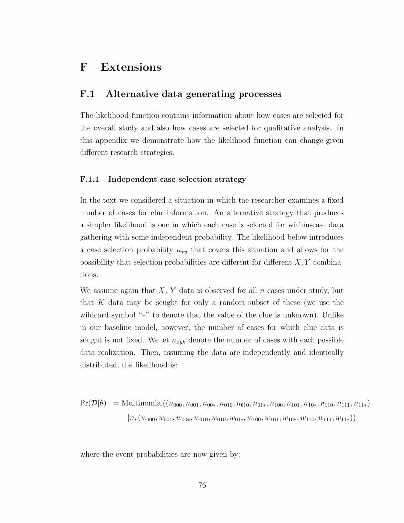
F Extensions

F.1 Alternative data generating processes

The likelihood function contains information about how cases are selected for

the overall study and also how cases are selected for qualitative analysis. In

this appendix we demonstrate how the likelihood function can change given

different research strategies.

F.1.1 Independent case selection strategy

In the text we considered a situation in which the researcher examines a fixed

number of cases for clue information. An alternative strategy that produces

a simpler likelihood is one in which each case is selected for within-case data

gathering with some independent probability. The likelihood below introduces

a case selection probability κxy that covers this situation and allows for the

possibility that selection probabilities are different for different X, Y combina-

tions.

We assume again that X, Y data is observed for all n cases under study, but

that K data may be sought for only a random subset of these (we use the

wildcard symbol “∗” to denote that the value of the clue is unknown). Unlike

in our baseline model, however, the number of cases for which clue data is

sought is not fixed. We let nxyk denote the number of cases with each possible

data realization. Then, assuming the data are independently and identically

distributed, the likelihood is:

Pr(D|θ) = Multinomial((n000, n001, n00∗, n010, n010, n01∗, n100, n101, n10∗, n110, n111, n11∗)

|n, (w000, w001, w00∗, w010, w010, w01∗, w100, w101, w10∗, w110, w111, w11∗))

where the event probabilities are now given by:

76

w000

w001

...

w11∗

=

λb(1− πb)κ00(1− φb0) + λc(1− πc)κ00(1− φc0)

λb(1− πb)κ00φb0 + λc(1− πc)κ00φc0...

λbπb(1− κ11) + λdπd(1− κ11)

We use a Greek symbol to denote the case selection probabilities to highlight

that these may also be unknown and an object of inquiry, entering into the

vector of parameters, θ.

F.1.2 Non-random XY Sample Selection

While we have assumed in our baseline model that cases are selected at random

for quantitative analysis, this need not be the case. Suppose instead that each

case of type j is selected into the study with probability ρj. In that situation,

assuming independent selection of cases for qualitative analysis, the likelihood

function is now:

Pr(D|θ) = Multinomial((n000, n001, n00∗, n010, n010, n01∗, n100, n101, n10∗, n110, n111, n11∗)

|n, (w000, w001, w00∗, w010, w010, w01∗, w100, w101, w10∗, w110, w111, w11∗))

where the event probabilities are now, given by:

w000

w001

...

w11∗

=

ρbλb

ρaλa+ρbλb+ρcλc+ρdλd(1− πb)κ00(1− φb0) + ρcλc

ρaλa+ρbλb+ρcλc+ρdλd(1− πc)κ00(1− φc0)

ρbλbρaλa+ρbλb+ρcλc+ρdλd

(1− πb)κ00φb0 + ρcλcρaλa+ρbλb+ρcλc+ρdλd

(1− πc)κ00φc0...

ρbλbρaλa+ρbλb+ρcλc+ρdλd

πb(1− κ11) + ρdλdρaλa+ρbλb+ρcλc+ρdλ11

πd(1− κ11)

We use a Greek symbol for the selection probabilities to highlight that these

probabilities may be unknown and could enter into the set of parameters of

77

interest, θ.

F.1.3 Conditional random case selection

Finally, consider the likelihood for a design in which a researcher selects cases

in which to search for clues as a function of the X, Y values. This is a somewhat

harder situation because the size of each X, Y group will be stochastic. Let

nxy = nxy0 + nxy1 + nxy∗ denote the number of cases with particular values on

X and Y , and let nXY = (n00, n01, n10, n11) denote the collection of nxy values.

Say now that, conditional on the X, Y observations, a researcher sets a target

of kxy(nXY ) cases for clue examination (note here that the number of clues

sought for a particular X, Y combination can be allowed to depend on what is

observed across all X, Y combinations). Then the likelihood is:

Multinomial(nXY |n,wXY )∏

x∈{0,1},y∈{0,1}

Binom(nxy1|kxy(nxy), ψxy)

The multinomial part of this expression gives the probability of observing the

particular X, Y combinations; the event probabilities for these depend on λ

and π only — for example w11 = λbπb + λdπd. The subsequent binomials give

the probability of observing the clue patterns conditional on searching for a

given number of clues (kxy(nxy)) and given an event probability ψxy for seeing

a clue given that the clue is sought for an x, y combination; thus for example:

ψ11 =λbπb

λbπb + λdπdφb1 +

λdπdλbπb + λdπd

φd1

F.2 Multiple Causes

Here we provide additional intuition for how the BIQQ framework can handle

multiple causal variables characterized by either equifinality (multiple poten-

tial causes of the same outcome) or interaction effects. The core approach is to

expand the number of types to take into account the more complex combina-

tions of causal conditions for which potential outcomes must now be defined.

78

Table 10 displays the set of potential outcomes for two binary causal variables.

With two causes, X1 and X2, we now have 16 types as defined by the potential

outcomes under alternative combinations of causal conditions.

Type Label (Y |X1 = 0, (Y |X1 = 1, (Y |X1 = 0, (Y |X1 = 1,X2 = 0) X2 = 0) X2 = 1) X2 = 1)

1 chronic 0 0 0 02 jointly-beneficial 0 0 0 13 2-alone-beneficial 0 0 1 04 2-beneficial 0 0 1 15 1-alone-beneficial 0 1 0 06 1-beneficial 0 1 0 17 any-alone-beneficial 0 1 1 08 any-beneficial 0 1 1 19 any-adverse 1 0 0 010 any-alone-adverse 1 0 0 111 1-adverse 1 0 1 012 1-alone-adverse 1 0 1 113 2-adverse 1 1 0 014 2-alone-adverse 1 1 0 115 jointly-adverse 1 1 1 016 destined 1 1 1 1

Table 10: Types given two treatments (or one treatment and one covariate)

Taking interaction effects first, Type 3 (2-alone-beneficial), for instance, is a

type in which X2 = 1 causes Y = 1 only when X1 = 0, and not when X1 = 1.

The hypothesis of no-interaction-effects is the hypothesis that all cases are of

type 1, 4, 6, 11, 13, or 16 (that is chronic, destined, 1-beneficial, 2-beneficial,

1-adverse, or 2-adverse). Note that the binary outcome framework excludes

possibilities, such as two countervailing or two additive effects of X1 and X2.

Turning now to equifinality, in the simple typological setup in the main paper,

the difference between a b and a d type already implies equifinality: for a b type,

the positive outcome was caused by treatment; for a d type, the same outcome

is caused by some other (unspecified) cause. Table 10, however, explicitly

builds multiple causes into the framework. Suppose, for instance, that we have

two cases, one of Type 4 and one of Type 6, and that X1 = X2 = 1 in both

cases. For both cases, we will observe Y = 1. However, for the Type 4 case,

79

the outcome was caused by X2 (in the sense that it would not have occurred if

X2 had been 0, but would have even if X1 was 0) whereas the outcome in the

Type 6 case was caused by X1, but not by X2.

The parameters in the model would now be defined in terms of these 16 types

and two causal variables.

For estimating population-level causal effects, we would state priors about the

population proportions of these 16 types.

Assignment probabilities would be expressed, separately for each independent

variable, as the probability that each type is assigned to the value 1 on that

variable, yielding 32 π values in total.

Clue probabilities, finally, would be supplied for each type. In principle, these

φ values could be made conditional on the combination of X1 and X2 values,

potentially yielding 64 φ values. In practice, greater structure might facilitate

analysis. For example, if a given clue’s likelihood depends only on the value of

one of the independent variables, rather than that of both, this greatly reduces

the required number of φ priors.

80

G Notes on Applications

G.1 Notes on Application 1

For the Kreuzer application we treat the φ values as known (or at least as

known with a very high level of certainty). Unfortunately we do not have, nor

do Kreuzer’s analyses provide, an empirical basis for claims about φ values.

Instead we present here an approach to “filling in the values” in the absence

of empirical information, based on reasoning about the theoretical logic and

background information about the world. The conclusions in the analysis can

be understood to be conditional on the phi values given below, though not on

the specific the reasoning that led to these values.

We begin with a few general comments:

– We refer throughout to the reasons for supporting PR that Boix (1999)

attributes to non-socialist parties under conditions of high left threat as

“electoral engineering” (EE) motives.

– We assume that there exist non-EE reasons why a governing coalition

of parties might prefer PR over single-member districts. These might

include, for instance, normative beliefs that PR is more democratic or a

response to mass demands for PR.

– We assume the socialist party never constitutes by itself a winning coali-

tion for enacting electoral reform, but that the non-socialist parties may

in some cases require socialist support to enact reform (see a-type cases).

– In our illustration, the “clue” is found if all three of the process-tracing

tests in Kreuzer (2010) are passed.

φa0 = 0.1: Probability of the clue for an untreated a type

An a (adverse) case is one in which strong left threat will prevent PR from being

adopted. We assume that adverse effects happen via the strategic calculations

and veto power of the left.

81

When the socialists are electorally strong and the right is divided, the left seeks

to stop any switch to PR since plurality rules now advantage them. Adverse

cases are those in which the non-socialist parties cannot enact electoral reform

without the support of the socialists — i.e., there the left has the institutional

leverage to veto a move to PR initiated by the right.

In an untreated “adverse” case (X = 0, Y = 1), the right does not have an EE

motive to favor PR. The left does favor PR for EE reasons, but by assumption

does not by itself form a winning coalition for enactment. Thus, PR must

emerge via support from non-socialist parties that is motivated by non-EE

reasons. However, PR can emerge without the support of all non-socialist

parties; all that is needed is some winning coalition.

The question for generating φa0, then, is in what proportion of untreated a

cases will all non-socialist parties favor a move to PR and do so shortly after

the expansion of the franchise. In other words, in what proportion of such cases

will there be non-EE motivations for PR that apply to all non-socialist parties

at this historical point in time, thus generating all three of Kreuzer’s clues?

Assuming that this is very unlikely, we assign a φa0 value of 0.1.

φa1 = 0.95: Probability of the clue for a treated a type

Under the adverse-effect logic above, we should see the clues in a treated a case

with a greater probability than in a treated b case (see below). This is because

there are two logics that might generate the clue in a treated a case.

1. In an a case with high left threat, right parties have the same EE incentives

that they do in a treated b case, where the clue probability is set at 0.9.

2. In addition, as explained for φa0, a cases are those in which a winning

coalition – which must include non-socialists – has non-EE reasons to

prefer PR. Further, we have assumed above that with 0.1 probability

those non-EE reasons apply to all non-socialist parties and emerge with

the expansion of suffrage, thus generating the clue.

82

We assume that reason 2 for the clue coexists with reason 1 in half of cases

with reason 2. Thus, the total probability of seeing the clue in a treated a type

is 0.9 + 0.1× 0.5 = 0.95.

φb0 = 0.1: Probability of the clue for an untreated b type

The lack of a left threat removes EE motives for the ruling parties under Boix’s

logic, thus reducing the likelihood of observing the clue in any untreated case.

Further, however, b (beneficial) cases are those in which no move to PR will

happen without high left threat. Thus, b cases are those in which there is also

no non-EE reason for adopting PR that obtains for any winning coalition of

parties.

Under Boix’s logic, therefore, it is very unlikely that we would see unanimous

non-socialist party support for a move to PR for a b case when left threat is

low. We thus set φb0 to 0.1, allowing only for a margin of measurement error.

φb1 = 0.9: Probability of the clue for a treated b type

A treated b case is one in which PR emerges under high left threat for precisely

the EE reasons that Boix outlines. As Kreuzer’s clues are tightly linked to

Boix’s logic, we place a high probability (0.9) on observing the clue for such

cases, allowing only for a margin of measurement error (e.g., the possibility

that we cannot find evidence of a right party’s support for PR even when that

support was in fact present).

φc0 = 0.05: Probability of the clue for an untreated c type

Cases of c (chronic) type are those in which PR will never emerge, even if left

threat is great. We posit that two processes may cause a case to be chronic:

1. Institutional obstacles: the right parties may prefer PR for EE or other

reasons, but some other actor has veto power over the decision. Here we

might observe the clue; or,

83

2. Preferences: a significant share of right parties have reasons, outside of

the logic of electoral engineering, for opposing PR. Here the clue should

never be observed.

We assume that each process is responsible for chronicness in 0.5 of all chronic

cases.

In an untreated case, there can be no EE reasons for the clue to emerge.

There could, however, be non-EE reasons for unanimous right-party support

in (and only in) the “institutionally” chronic cases. We have assumed that

0.5 of chronic cases are “institutional.” Then, consistent with the assumptions

made for a cases about the prevalence of non-EE reasons, we posit that in

0.1 of all “institutional” chronic cases, there are non-EE reasons that generate

unanimous right-party support for PR.

The total probability of observing the clue in an untreated c case, then, is

0.1× 0.5 = 0.05.

φc1 = 0.475: Probability of the clue for a treated c type

In treated chronic cases of the “preference” variety (0.5 of c cases), the clue

will never emerge.

However, there are two ways in which the clue could emerge in institutionally

chronic cases:

1. As discussed above, 0.1 of such cases will have non-EE reasons for gener-

ating the clue.

2. In addition, however, in a treated institutionally Chronic case, the clue

could emerge via the same logic that generates EE motives in 0.9 of treated

b cases.

As we do for treated a cases, we assume that reason 2 for the clue coexists

with reason 1 in half of cases with reason 2. We thus get 0.95 of institutionally

chronic cases having the clue, giving φc1 = 0.5× 0.95 = 0.475.

84

φd0 = 0.3: Probability of the clue for an untreated d type

In d (destined) cases, PR will always emerge, regardless of whether left threat

is high.

This means that in d cases some winning coalition always has a non-EE reason

sufficient to support PR. This coalition might:

1. include a unified right and take place at the time of suffrage expansion,

in which case we will observe the clue, or

2. be a coalition of part of the right and the left or happen at some other

time, in either of which case we will not observe the clue.

So the question is: how common will situation 1 be in d cases? Since d cases are

those that always generate PR, we assume that this is because the normative

and other non-EE pressures to adopt PR are inherently stronger in these cases

than in the other types. We thus assume a higher probability that such pres-

sures will apply to all non-socialist parties, and we posit that such pressures

are likely to be strongest of all at the “democratic moment” that produces the

universal male franchise.

We thus put the probability of observing the clue in such a case at the low-

moderate value of 0.3.

φd1 = 0.5: Probability of the clue for a treated d type

We see two processes that might produce the clue in a treated d case.

1. In a d case, any EE motives for supporting PR must be causally redun-

dant: there must be a winning coalition for PR for reasons outside Boix’s

framework. As discussed for untreated d cases, any winning coalition gen-

erated by non-EE reasons might not include all right parties. We have

assumed above that non-EE reasons affect all non-socialist parties follow-

ing the suffrage expansion, and thus produce the clue, in 0.3 of cases.

85

2. At the same time, in a treated d case some EE strategic considerations

may also operate on right parties. Thus, high left threat in a d case may

bring the remaining right parties (those unmoved by non-EE motives) into

support of PR, generating the clue. We assume that this configuration is

relatively rare, obtaining in 0.2 of cases.

We add the probabilities of the two processes together, yielding φd1 = 0.3 +

0.2 = 0.5.

G.2 Notes on Application 2

G.2.1 Case selection

To integrate the inferences from Ross’s (2004) analysis with the wider Collier

and Hoeffler (2004) population of cases we faced two challenges that affected

the set of cases that we could use for this analysis.

First, we had to create a binary measure of natural resource wealth. This is

done implicitly in Ross’s analysis but not explicitly. Consulting Collier and

Hoeffler’s data, we could find no threshold that separated cases with high and

low levels of natural resources consistent with Ross’s analysis. Most cases

in the Ross sample had relatively high levels of natural resources, but one,

Afghanistan, did not — even though experts linked natural resources to the

conflict in this case. This coding raises a subtle issue: it is possible that X is

causally linked to Y in a given case even though X takes on an exceptionally low

value in the case. Should such a case count as evidence that natural resource

wealth causes conflict or not? We take it that the general proposition X causes

Y should be interpreted as a claim that some minimal level of X causes Y .

Under this reading cases with very low levels of X in which Y = 1 are not

supportive of the proposition that X causes Y , even if paths can be found

between X and Y . Under this interpretation, we selected a threshold level of

resource dependence that separated cases in a way as consistent with Ross’s

coding as possible; in doing so we were forced to omit Afghanistan from the

qualitative analysis.

86

Second, we had to identify the population of cases from which Ross’s subset

were drawn. We discuss one selection criterion used by Ross — expert judg-

ments — in the main text. A second selection criterion for Ross was the timing

of the conflicts. Ross selected cases of conflicts that started or were ongoing

in a given time period. Including cases that began before the period in ques-

tion, on the grounds that they had a conflict that continued into the period,

makes identification of the population of cases difficult because we do not know

whether a given case that did not have a conflict prior to the period would have

had a conflict long enough to take it into the sample, conditional on having

had a conflict. To deal with this problem, we limited the population to all

cases in which there was not a conflict ongoing in the 1990s and interpreted

the outcome variable as an indicator of a conflict start in this period.

G.2.2 Probative values of clues and graphical representation of pos-

teriors

For our analyses we considered two sets of values (informative and uninfor-

mative) for each of two types of clue, K1 and K2. For K1 uninformative, we

supposed that φ1b1 = φ1

d1 = 0.5; for K1 informative, we set φ1b1 = .9, φ1

d1 = 0.3,

making clue 1 a strong (i.e., difficult) hoop test. For K2 uninformative, we sup-

posed that φ2b1 = φ2

d1 = 0.5; for K2 informative, we set φ2b1 = .99, φ2

d1 = 0.01,

making clue 2 strongly doubly decisive.

In the text we provide summary statistics of the posterior distributions un-

der these different assumptions of the informativeness of the clues. Figure 7

presents information on these posteriors graphically for each set of assumptions.

87

−0.6 −0.4 −0.2 0.0 0.2 0.4 0.6

0.0

0.2

0.4

0.6

0.8

1.0

Posteriors | Both clues weak

ate (posterior mean = −0.017 )

Asi

gnm

ent p

rope

nsity

for

c ty

pes

−0.6 −0.4 −0.2 0.0 0.2 0.4 0.6

0.0

0.2

0.4

0.6

0.8

1.0

Posteriors | Both clues strong

ate (posterior mean = −0.002 )A

sign

men

t pro

pens

ity fo

r c

type

s

Figure 7: Joint distribution of posterior beliefs on the average effect of natural re-sources on conflict (i.e., λb − λa) and the beliefs regarding differential assignmentprobabilities, given clues of varying probative value. Plots also show the marginalposterior on the average causal effect.

H Notes on Simulations

Here we provide statistical details and some further interpretation for the pa-

per’s simulations assessing the benefits of different designs conditional on dif-

ferent priors on: the probative value of clues, the heterogeneity of causal effects,

uncertainty regarding assignment probabilities, and uncertainty regarding the

probative value of clues. Table 11 provides details on all parameters used in

simulations; Table 12 provides detail on the number of runs, iterations, and

related information used in the estimation.

H.1 Probative values

For these simulations we simultaneously vary the probative value for tests for

all X, Y combinations. Specifically, we vary the differences between φb0 and φc0

(for X = Y = 0 cases), between φa0 and φd0 (for X = 0, Y = 1 cases); between

φa1 and φc1 (for X = 1, Y = 0 cases); and between φb1 and φd1 (for X = Y = 1

88

cases). For each X, Y combination, we compare the relevant φ pairs across

values of (.5, .5) (no probative value), (.25, .75) (middling probative value) and

(0.01, 0.99) (strong probative value). Using the definition of probative value

(PV) (see footnote 5), these correspond to cases with probative value of 0, .5,

and close to 1 respectively.

H.2 Effect heterogeneity

We note that heterogeneity makes going “wide” relatively more beneficial for

two reasons. First, when all cases are affected either positively or negatively,

all of the information needed to identify types is provided by information on

X and Y . If X = Y , then a case was (or could have been) positively affected;

if X 6= Y then a case was (or could have been) negatively affected. In this

extreme case of maximal heterogeneity, causal process information provides no

additional inferential gains. Where there is high homogeneity, on the other

hand, the core difficulty is distinguishing a and b types, from c and d types.

Then, the information contained in clues may provide greater benefits (see

Table 2). Second, the more heterogeneous effects are across cases, the less we

learn about population-level causal effects by getting an individual case right.

Thus, again, we would expect greater relative gains to more extensive analysis

as heterogeneity increases.

H.3 Uncertainty about assignment processes

Note that in our binary setup, infinite bias cannot arise, and the harm done

by uncertainty over selection processes can be more moderate. In this set of

simulations, the expected value of πj is fixed at 0.5 and we vary the variance

in πj between 0 and a maximum of 0.289.

H.4 Uncertainty regarding the probative value of clues

In this experiment, the expected probability that a clue will be observed is

set to 0.85 if one hypothesis is right, and 0.15 if the alternative hypothesis is

89

correct. The simulations vary from a situation in which those probabilities are

known with certainty (uncertainty low) to a situation in which the researcher

admits the possibility of many possible values of φ. Uncertainty is simultane-

ously varied for all pairs of φ values (see §H.1). The displayed results suggest

that uncertainty about the probative value of clues plays a muted role in the

assessment of optimal strategies.

H.5 Details on simulation experiments

90

1:

mor

n2:

Pro

bat

ive

Val

ue

3:E

ffec

tH

eter

ogen

eity

4:A

ssig

nm

ent

Un

cert

ain

ty5:

Clu

eU

nce

rtain

ty

θD

ist

arg

Low

→H

igh

Low

→H

igh

Low

→H

igh

Low

→H

igh

λa

Dir

ich

let

αa

10.

20→

0.20

0.10

→2.00

1→

11

→1

λb

αb

10.

20→

0.20

02.1

0→

4.00

1→

11

→1

λc

αc

10.

20→

0.20

02.0

0→

0.10

1→

11

→1

λd

αd

10.

20→

0.20

02.0

0→

0.10

1→

11

→1

πa

Bet

aµ

0.50

0.50→

0.50

0.50

→0.

500.

50→

0.50

0.5

0→

0.5

0σ

0.10

0.10→

0.10

0.10

→0.

100.

01→

0.289

0.1

0→

0.1

0

πb

Bet

aµ

0.50

0.50→

0.50

0.50

→0.

500.

50→

0.50

0.5

0→

0.5

0σ

0.10

0.10→

0.10

0.10

→0.

100.

01→

0.289

0.1

0→

0.1

0

πc

Bet

aµ

0.50

0.50→

0.50

0.50

→0.

500.

50→

0.50

0.5

0→

0.5

0σ

0.10

0.10→

0.10

0.10

→0.

100.

01→

0.289

0.1

0→

0.1

0

πd

Bet

aµ

0.50

0.50→

0.50

0.50

→0.

500.

50→

0.50

0.5

0→

0.5

0σ

0.10

0.10→

0.10

0.10

→0.

100.

01→

0.289

0.1

0→

0.1

0

φa0

Bet

aµ

0.01

0.50→

0.01

0.01

→0.

010.

01→

0.01

0.1

5→

0.1

5σ

0.01

0.01→

0.01

0.01

→0.

010.

01→

0.01

0.0

005→

0.0638

φa1

Bet

aµ

0.99

0.50→

0.99

0.99

→0.

990.

99→

0.99

0.8

5→

0.8

5σ

0.01

0.01→

0.01

0.01

→0.

010.

01→

0.01

0.0

005→

0.0638

φb0

Bet

aµ

0.01

0.50→

0.01

0.01

→0.

010.

01→

0.01

0.1

5→

0.1

5σ

0.01

0.01→

0.01

0.01

→0.

010.

01→

0.01

0.0

005→

0.0638

φb1

Bet

aµ

0.99

0.50→

0.99

0.99

→0.

990.

99→

0.99

0.8

5→

0.8

5σ

0.01

0.01→

0.01

0.01

→0.

010.

01→

0.01

0.0

005→

0.0638

φc0

Bet

aµ

0.99

0.50→

0.99

0.99

→0.

990.

99→

0.99

0.8

5→

0.8

5σ

0.01

0.01→

0.01

0.01

→0.

010.

01→

0.01

0.0

005→

0.0638

φc1

Bet

aµ

0.01

0.50→

0.01

0.01

→0.

010.

01→

0.01

0.1

5→

0.1

5σ

0.01

0.01→

0.01

0.01

→0.

010.

01→

0.01

0.0

005→

0.0638

φd0

Bet

aµ

0.99

0.50→

0.99

0.99

→0.

990.

99→

0.99

0.8

5→

0.8

5σ

0.01

0.01→

0.01

0.01

→0.

010.

01→

0.01

0.0

005→

0.0638

φd1

Bet

aµ

0.01

0.50→

0.01

0.01

→0.

010.

01→

0.01

0.1

5→

0.1

5σ

0.01

0.01→

0.01

0.01

→0.

010.

01→

0.01

0.0

005→

0.0638

Tab

le11

:S

imu

lati

onp

aram

eter

s.E

ach

colu

mn

det

ail

sp

ara

met

ers

use

dto

gen

erate

pri

or

dis

trib

uti

on

sfo

ron

eof

the

sim

ula

tion

sb

elow

.T

he

pri

ord

istr

ibu

tion

for

the

full

par

amet

erve

ctor

isfo

rmed

from

ind

epen

den

td

raw

sfr

om

Bet

ad

istr

ibu

tion

sfo

rall

pro

bab

ilit

ies

an

dth

eD

iric

hle

td

istr

ibu

tion

for

shar

es.

Not

eth

atth

em

ean

an

dst

an

dard

dev

iati

on

para

met

eriz

ati

on

we

pro

vid

efo

rB

eta

dis

trib

uti

on

sca

nb

em

app

edd

irec

tly

toth

em

ore

stan

dar

dα,β

para

met

eriz

ati

on

.F

or

the

Clu

eU

nce

rtain

tyex

per

imen

tsth

ep

ara

met

ers

corr

esp

on

dto

ash

ift

from

Beta(.

15×

2i,.

85×

2i )

fori∈{0,4,8}.

91

j steps k simsExperiment per exp. per step Comments1: Varying N or m 29 5,200 The 5,200 k simulations for each θj were split into

26 runs of 200 k sims, and then compiled throughaveraging.Datapoints at N=3 and N=4 were added using14,200 k simulations.

2: Probative Value 30 5,200 The 5,200 k simulations for each θj were split into26 batches of 200 k sims, and then compiled throughaveraging.

3: Effect Heterogeneity 30 5,200 The 5,200 k simulations for each θj were split into26 batches of 200 k sims, and then compiled throughaveraging.

4: Assignment Uncertainty 30 5,200 The 5,200 k simulations for each θj were split into26 batches of 200 k sims, and then compiled throughaveraging.

5: Clue Uncertainty 30 10,200 The 10,200 k simulations for each θj were split into26 batches of 200 k sims and 10 batches of 500, thencompiled through averaging.

Table 12: Note: Each experiment takes j steps through different values of θ. At each θj , the datais simulated k times. For each simulation, a call is made to the Stan model and HMC (HamiltonianMonte Carlo) sampling is used to approximate the posterior distribution. In each such call to Stan,we run 4 chains with 6000 iterations, and 1000 warmup draws.

92

I Learning from non-discriminating clues

We noted in the text that when priors over clue probabilities do not discriminate

between causal types, then learning clue values does not affect learning over

other parameters when n = 1. However, learning is possible for n > 1 even

when priors over clue probabilities do not discriminate between causal types.

To see why, divide θ into two parts, θ−φ and θφ, where θ−φ denotes the vector

of parameters excluding {φjx}j∈{a,b,c,d},x∈{0,1}, and θφ the complement.

We represent non-discriminating priors over the clues probabilities as follows.

Assume that the prior distribution over θ is given by p(θ−φ)∏

j∈{a,b,c,d},x∈{0,1} f(φjx)

— thus the marginal prior distribution over each φjx, j ∈ {a, b, c, d}, x ∈ {0, 1}is given identically by some distribution f . Thus for this claim the key feature

is not that f is flat, but simply that it is the same for different causal types.

We consider a situation in which we observe X = Y = K = 1 for a case and

show that the posterior distribution over θ−φ is the same as it would be if we

observed X, Y , data only. The same analysis can be conducted for any other

combination of X, Y data.

With X = Y = K = 1 the posterior marginal distribution is:

p(θ−φ|X = Y = K = 1) =

∫ ∫((λbπbφb1 + λdπdφd1) p(θ−φ)f(φb1)f(φd1)) dφb1dφd1∫ ∫ ∫(λbπbφb1 + λdπdφd1)p(θ−φ) f(φb1)f(φd1)dθ−φdφb1dφd1

=

(λbπb

∫φb1f(φb1)dφb1 + λdπd

∫φd1f(φd1)dφd1

)p(θ−φ)∫ (

λbπb∫φb1f(φb1)dφb1 + λdπd

∫φd1f(φd1)dφd1

)p(θ−φ)dθ−φ

Since∫φb1f(φb1)dφb1 =

∫φd1f(φd1)dφd1 , this simplifies to the posterior that

obtains when information on K is disregarded entirely:

(λbπb + λdπd) p(θ−φ)∫(λbπb + λdπd) p(θ−φ)dθ−φ

93

A critical step in this simple proof is our ability to move the integrals given

the fact that the φ terms enter the likelihood in an additive way.

This is not the case for n > 1. For example say there were two cases, each with

X = Y = K = 1 we would then have:

p(θ−φ|X = Y = K = (1, 1)) =

∫ ∫ ((λbπbφb1 + λdπdφd1)

2 p(θ−φ)f(φb1)f(φd1))dφb1dφd1∫ ∫ ∫

(λbπbφb1 + λdπdφd1)2p(θ−φ) f(φb1)f(φd1)dθ−φdφb1dφd1

which does not admit the same simplification. For a counterexample, suppose

that the only parameters over which there is uncertainty are λb, φb1 and φd1.

Assume that f() is uniform, that priors over λb are also given by a uniform

distribution over [0, 1], that λd = 1 − λb, and that πb = πd. Note that in this

simple world, observing two instances of X = Y = 1 does not provide informa-

tion on whether b types are more or less common than d types since conditional

on X = 1 both types produce Y = 1 (equivalently, both types produce data

like this with probability πb, πd). The question is whether information on K

can shift beliefs even though there is no prior information to lead one to expect

K to be observed with greater probability for a b or a d type. The posterior

marginal distribution over λb is now:

p(λb|X = Y = K = (1, 1)) =

∫ ∫(λbφb1 + (1− λb)φd1)2 dφb1dφd1∫ ∫ ∫

(λbφb1 + (1− λb)φd1)2dλbdφb1dφd1

Solving out yields:

p(λb|X = Y = K = (1, 1)) =6(2 + λ2b − λb)

11

This symmetric U-shaped posterior distribution suggests that observing K does

not shift the expected share of b and d types in this situation. It does, however,

result in greater weight placed on extreme values of λb — that is, after seeing

the data, we now believe that it is more likely that there are either very many

94

or very few b types. Intuitively, the discrimination arises because, given the

independent priors on φb and φd, it is more likely that clue probabilities are

high for one type than that they are high for two types.

J Maximum Likelihood Integration

Although we favor a Bayesian approach to integrating inferences from qualita-

tive and quantitative data, we note that a similar approach can be implemented

within a maximum likelihood framework. The key point is that information on

the probative value on clues places a structure on the likelihood which affects

inferences under both a Bayesian and a maximum likelihood analysis.

We illustrate here with an example that imposes considerable structure on the

likelihood.

Suppose that it is known for certain that there are only b and d types in a

population and that a clue K is observed with probability q if the unit is a b

type in treatment, and with probability zero otherwise (we use q rather than

φ to highlight the fact that in this example probative value is given and is not

a parameter to be estimated). Say, moreover, that all types are assigned to

treatment with probability .5.

In that case data can be summarized by a vector (n00, n01, n110, n111) and the

likelihood of the data is given by:

L =n!

n00!n01!n110!n111!(.5λb)

n00(.5(1−λb))n01(.5λb(1−q)+.5(1−λb))n110(.5λbq)n111

and so:

L ∝ λn00+n111b (1− λb)n01(1− qλb)n110

The maximum likelihood estimate (MLE) is the maximum of the log likelihood:

max ((n00+n111) ln(λb) + n01 ln(1− λb) + n110 ln(1− qλb))

95

First-order conditions are:

n00 + n111

λb− n01

1− λb− qn110

1− qλb= 0

The second-order condition is satisfied since:

−n00 + n111

λ2b− n01

(1− λb)2− q2 n110

(1− qλb)2< 0

We note that if there is only one case or one sort of case (e.g., only X = Y =

K = 1 cases), then the first-order condition cannot be satisfied: the maximum

is at the boundary. An implication of this is that, for single-case analysis, the

MLE estimate can be insensitive to the probative value of clues.

For illustrative purposes, suppose n01 = n00 = n110 = n110 > 0. Then the first

order condition is satisfied uniquely23 by:

λ∗b =3(q + 1)−

√9(q + 1)2 − 32q

8q

This solution falls from λb = 23

to λb = 12

as q varies from 0 to 1. These

differences reflect the fact that in this example the n111 X = Y = K = 1 cases

and the n00 X = Y = 0 cases are known to be b types; and the n01 cases with

X = 0, Y = 1 are known to be d types. The only uncertainty arises for the

n110 cases with X = Y = 1 and K = 0. If b types have a low probability of

exhibiting the clue when X = 1, then many of these cases are likely to be b

types.

23A second solution exists but exceeds 1 for admissible values of q.

96