mittal effects of market capitalization ratio on gdp ... gdp growth and capital market robustness in...

The Effects of Market Capitalization Ratio on GDP Growth and Capital Market Robustness in Newly Industrialized

Countries

Rishab Mittal1

The objective of this study is to explore the presence of a causal relationship between stock market

development and economic growth. This study aims to explore this relationship in the nine Newly Industrialized Countries (NIC’s): Brazil, China, India, Malaysia, Mexico, Philippines, South Africa, Thailand and Turkey. 2005 nominal GDP values are used as a proxy for economic growth, and market capitalization ratio (MCR) is used as a proxy for stock market development.

To address this relationship, a Granger Causality Test was employed. However, before running a Granger Causality test, it must be determined whether the variables are stationary and, if not, whether they are co-integrated. To test whether variables are stationary, an augmented Dickey-Fuller unit root test (ADF) was employed. All of the countries rejected the null except for Mexico. Following an ADF test, an Engle-Granger Co-integration test (Engle test) was employed. Mexico failed to reject the null for the Engle test; thus no accurate conclusions for Mexico can be made following this study. Finally, the Granger Causality Test can be employed. Results show bi-directional causality for China, Thailand and Turkey between GDP and MCR. Uni-directional causality for MCR to GDP exists for India and Mexico. Uni-directional causality for GDP to MCR exists for Malaysia, the Philippines and South Africa. No causality is determined for Brazil. The results show that the financial markets are important for economic growth in India, Mexico, China, Thailand and Turkey. It is important to remember that this causal relationship is country specific. Therefore, a general statement cannot be made that the stock market causes economic growth.

1 Rishab Mittal is a member of the class of 2017 at the University of Chicago.

UChicago Undergraduate Business Journal

Spring 2014 1

Introduction

The economy plays a large part in any society and therefore touches upon a multitude of sectors within a

country. Some of the main sources of economic growth are population, industry, the stock market, as well as

politics. A well-developed stock market should promote growth by encouraging increased savings and lowered

transaction costs (Dicle 2010). The market capitalization over GDP ratio shows the growth of the stock market

relative to the GDP. Market capitalization to GDP ratio and turnover to market capitalization ratio are higher in

higher income countries (Filer 1999). Higher income countries have more developed financial institutions, meaning

a well-developed bond and equity market. With credit generally better available in such an economy, higher income

countries generally experience more growth. However, Newly Industrialized Countries (NIC) is a special group of

countries classified as anomalies to this concept (Pal 2006).

In addition, human capital is an important determinant of long run economic growth (Cooray

2010). Human capital is defined to be the quality of the workforce in an economy that produces economic

value, i.e., earnings potential. In general, human capital is higher in developed countries due to a number

of factors: quality of education, GDP per capita, and available facilities (Durham 2002). Foreign portfolio

investment2has also been shown to have a positive impact on the growth of developing countries. During

the 1980s and 1990s, Foreign Portfolio Investment (FPI) emerged as an important form of capital inflow

to developing countries (Pal 2006). Hence, a number of variables must be accounted for when analyzing

catalysts of economic growth.

This research primarily focuses on the stock market. Stock market growth can be measured by

three variables: market capitalization over GDP, turnover velocity and change in the number of domestic

shares listed (Randall et al, 1999). As stated above, these are usually prodigious in a developed economy,

thus galvanizing strong economic growth. By offering a wide array of financial assets, financial institutions

stimulate savings (Patrick, 2007). A well-developed financial system consists of a wide variety of financial

assets, such as bonds, stocks and bank deposits. However, developing countries generally do not have very

large bond markets, which is one of the main reasons why they are classified as developing countries (Deb

2008).

In addition, more liquid assets and easy access to capital markets can improve allocation of capital,

while market volatility can increase the number of shares bought and sold (Arestis 2001). Both of these, in

turn, are good for the economy because they increase buyer confidence. A volatile market experiences high

fluctuation in share prices and can often be riskier for trading. But high risk results in higher returns of

investments and often complex trading algorithms can assess the risk in a volatile market. Oftentimes, due

to the possible high return, traders like to trade in a volatile market, thus stimulating stock market growth

(Patrick 2005).

2 Foreign portfolio investment (FPI) generally consists of securities and other financial assets held by foreign investors. They do not provide the investor with direct ownership of financial assets, and thus do not entail control over management. FPI is generally thought to be liquid, depending on the volatility of the market invested in.


Spring 2014 2

Researchers and analysts have conflicting views when it comes to the effect of the stock market on

economic growth. Evidence shows that in some countries economic growth systematically causes financial

development (Demetriades 1996). However, stock market development may hamper economic growth if it

is at the expense of banking system development (Arestis 2001).

India, a new member of the NIC, is one of the fastest growing countries today and can be used to

represent the lower income countries. Other NIC countries as of June 2011 include: Brazil, China, Mexico,

South Africa, Turkey, Mexico, Malaysia and Thailand. As noted, a strong relationship between stock market

activity and future economic growth exists for lower income countries but not higher income countries

(Cooray 2010). These countries are experiencing better economic growth than that of other developing

countries, yet have still not met the standard requirements for being classified as a developed country

(Cooray 2010). Countries in their early stage of development benefit more from financial sector

development than their older and mature counterparts (Mukherjee 2008). India’s market capitalization to

GDP ratio has increased from 5.76 % in 1982 to 47.59 % in 2003 (Pal 2006). This growth shows how much

the stock market has appreciated in aggregate value over the last twenty years compared to the economy.

India’s expeditious growth in its stock market over the last two decades has greatly helped develop the

country’s economy (Deb. 2008).

According to Harris, the link between stock markets and growth only exists for developed

countries (Harris 1997). But, due to the ambiguity of the causality, a voluminous amount of literature has

refuted the statement that stock market growth causes economic growth. Arestis et al. (2001) argue that

both banks and stock markets lead to increased growth, but banks have a greater influence in promoting

economic growth. Although, Atje and Javanovic (1993) concluded that the stock market leads to greater

economic growth.

Additionally, stock market development exacerbates macroeconomic instability and does not lead

to economic growth in developed countries (Singh 1997). Similarly, Devereux and Smith (1994) suggest that

the stock market’s minimal role in the economy can lead to reduced risk—and subsequently larger

economic growth. For the United States, capital market development has no causal effect on the GDP and

banking sector development (Arestis 2001). This is contrary to Cooray’s argument that human capital is an

important determinant of long run economic growth.

Though population growth may have a negative influence on economic growth (Cooray 2010),

India and China have experienced continuous growth along with exponential population growth in the last

few decades. (Dicle 2010). A few things can explain this growth. Financial development can be proxied by

the ratio of liquid liabilities (M3) to GDP. The growth of M33 and MCR are two major sources of growth in

3 Liquid liabilities (M3), are also known as broad money. They are the sum of currency and deposits in the central bank (M0), plus transferable deposits and electronic currency (M1), plus time and savings deposits, foreign currency transferable deposits, certificates of deposit, and securities repurchase agreements (M2), plus travelers checks, foreign currency time deposits, commercial paper, and shares of mutual funds or market funds held by residents.


Spring 2014 3

any economy (Dawson 2008). Liquid liabilities are a percent of the GDP and therefore provide a good

estimate for the direction of the economy. These fundamental relationships in macroeconomics provide the

foundations of this research.

The performance of the stock market and its impact on an economy can be seen through a variety

of factors. Though there is much debate on whether the stock market causes economic growth, a positive

correlation can be seen in a number of the NICs (Filer 1999). Whether or not the financial market plays a

causal role on economic growth is still under question. The majority of the evidence shows a positive

impact of stock market growth on per capita GDP, human capital growth, and credit risk (Durham 2002).

This research seeks to provide conclusive evidence that stock market development is indeed one cause of

economic growth in the NIC countries.

Null Hypothesis (Ho): In the following NIC countries—Mexico, Brazil, China, India, South

Africa, Philippines, Thailand, Malaysia and Turkey—there is no bi-directional causal relationship between

market capitalization over GDP and GDP that explains economic growth over two different decades

(1990s and 2000s).

Alternative Hypothesis (Ha): In the following NIC countries—Mexico, Brazil, China, India, South

Africa, Philippines, Thailand, Malaysia and Turkey—there is a bi-directional causal relationship between market

capitalization over GDP and GDP that explains economic growth over two different decades (1990s and

2000s).

Methodology and Data Measurement

Market capitalization over GDP ratio (MCR) data was collected for the nine NIC countries using

WorldBank.org. 2005 nominal GDP values were collected. This data spanned two decades (1990-2010). The 2005

real GDP nominal values are used as a proxy for economic growth. This data was imported into Excel, and a

least squares regression line for each country was run to calculate the r-squared value between GDP vs. MCR. In

addition, a time series graph4 was used to compare the two data sets relative to each other. The graphs included

two y-axes sharing one x-axis, time (in years). After recording trends in the data set, causality can be tested.

Thereafter, a Granger causality test was conducted in R. The null hypothesis is that the y does not

Granger cause x. A user specifies the two series, x and y, along with the significance level and the maximum

number of lags to be considered. The function produces the F-statistic5 for the Granger causality test along with

the corresponding p-value6. The null hypothesis, y does not Granger Cause x, is rejected if the F- statistic is

greater than the critical value. A Granger causality test with 1, 2, 3, 4 and 5 maximum lags7 for each country was

4 A time series graph is a graph with y vs. time (sometimes there can be two variables on the vertical axis, as was the case in the time series graphs I conducted. 5 The F-statistic is what is produced by the Granger Causality test. Each F-statistic has a corresponding p-value 6 The p-value is the probability of the null hypothesis coming true. Remember, the null hypothesis is the opposite of what you are trying to prove, so the smaller the p-value, the more statistically significant the data. 7 A lag is when you compare y and x from different time periods. Lags are important in economic data due to the time (or lag)


Spring 2014 4

conducted, and the F-statistic and p-value for MCR vs. GDP and GDP vs. MCR was recorded. This was done

for each of the nine countries. Lags are important when dealing with economic data because government fiscal

policies tend to take a number of years to take into effect. Thus, lags take this delayed change into account.

In addition, an augmented Dickey-Fuller (ADF) unit root test was conducted. A unit root test is used to

find whether a time series variable, such as GDP, is non-stationary. If a unit root is present, the variable is non-

stationary. The null hypothesis is that the unit root exists, and the alternative hypothesis is that the unit root does

not exist. The variables need to be stationary in order for the Granger causality test to be reliable. To conduct a

unit root test, codes were inserted into R to create a function to conduct the ADF test.

Finally, an Engle-Granger test is conducted to test whether the data is co-integrated. The null is that

there is no co-integration. The variables must be co-integrated for the Granger causality test to be accurate.

Results

Brazil (Table 1), China (Table 2), India (Table 3), Malaysia (Table 4), Philippines (Table 6), South Africa

(Table7), Thailand (Table 8) and Turkey (Table 9) are all statistically significant at the 1% level for the unit root

test. Therefore, there is strong evidence to reject the null hypothesis and conclude that the variables are

stationary. In addition, each one of these countries has a very strong R-squared value of approximately 0.90 and

above. This is in strong correlation to the small p-values obtained. Mexico, with a p-value of 0.11, does not have

statistically significant data, thus it fails to reject the null hypothesis (Table 5). A unit root exists. In addition, its

R-squared value is a meager 0.71 compared to the other countries.

After the ADF test, an Engle and Granger Co-integration Test (Engle test) was employed. The null

hypothesis for this test is that the variables are not co-integrated, and the alternative is that the variables are co-

integrated. Co-integration of variables is important because that makes the F-test in the Granger Causality test

reliable. Without co-integration, the F-test in the Granger Causality test may not be reliable in forecasting future

values.

The results for the Engle test are as follows: Brazil, China, India, Malaysia, South Africa, and Turkey all

have statistically significant results at the 1% level except for Malaysia (significant at the 10% level). Mexico,

Philippines and Thailand all have too high p-values, thus the null hypothesis fails to be rejected (Table 5b, 6b,

and 8b respectively). But, since the variables for Thailand and the Philippines are stationary, the Granger

Causality test can be reliable. Since both the unit root test and Engle test fail for Mexico, the results of Mexico in

this study cannot be relied upon. With non-stationary data and non-co-integrated variables, a standard

regression, which is what the Granger Causality Test is based on, can lead to a relationship between the two

variables that do not actually exist. This concept is called a spurious regression.

Finally, a Granger Causality Test can be employed. The test was conducted for lags 1-5 and conducted

in both ways. The null hypotheses were as such:

it takes for policy changes effected by the government to start impacting the economy.


Spring 2014 5

1. MCR does not Granger cause GDP.

2. GDP does not Granger cause MCR.

The Granger Causality test gives an F-statistic and p-value for each lag length, which can be used to

make conclusions.

The results for the test are as follows: For null hypothesis one, statistically significant data was found for

China (1% at 5 lags), India (10% at 1 lag), Mexico (1% at 2 lags), Thailand (10% at 2 lags), and Turkey (1% at 2

lags) (Table 2c, 3c, 5c, 8c, and 9c respectively). For null hypothesis two, statistically significant data was found for

China (10% at 1 lag), Malaysia (10% at 2 lags), Philippines (10% at 1 lag), South Africa (10% at 2 lags), Thailand

(10% at 2 lags), and Turkey (5% at 2 lags).

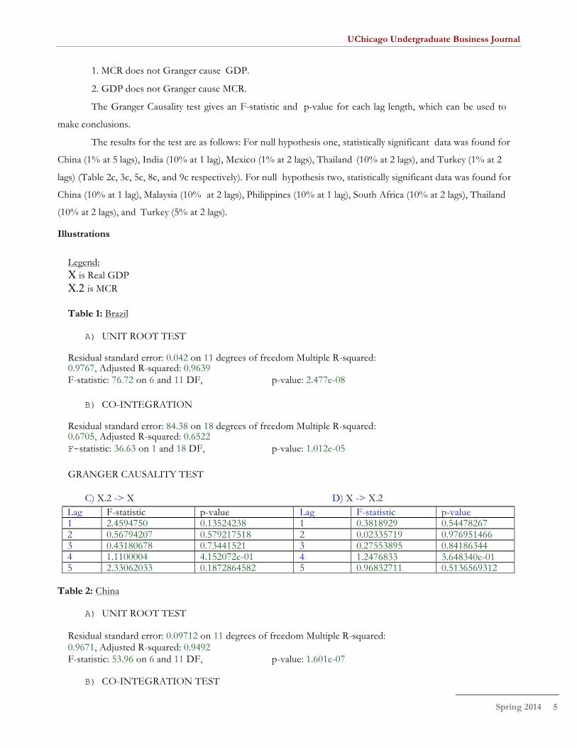
Illustrations

Legend: X is Real GDP X.2 is MCR

Table 1: Brazil

A) UNIT ROOT TEST

Residual standard error: 0.042 on 11 degrees of freedom Multiple R-squared: 0.9767, Adjusted R-squared: 0.9639 F-statistic: 76.72 on 6 and 11 DF, p-value: 2.477e-08

B) CO-INTEGRATION

Residual standard error: 84.38 on 18 degrees of freedom Multiple R-squared: 0.6705, Adjusted R-squared: 0.6522 F- statistic: 36.63 on 1 and 18 DF, p-value: 1.012e-05

GRANGER CAUSALITY TEST

C) X.2 -> X D) X -> X.2 Lag F-statistic p-value Lag F-statistic p-value 1 2.4594750 0.13524238 1 0.3818929 0.54478267 2 0.56794207 0.579217518 2 0.02335719 0.976951466 3 0.43180678 0.73441521 3 0.27553895 0.84186344 4 1.1100004 4.152072e-01 4 1.2476833 3.648340e-01 5 2.33062033 0.1872864582 5 0.96832711 0.5136569312

Table 2: China

A) UNIT ROOT TEST


B) CO-INTEGRATION TEST


Spring 2014 6



C) X.2 -> X D) X -> X.2 Lag F-statistic p-value Lag F-statistic p-value 1 0.46972441 5.023535e-01 1 4.21776317 5.571574e-02 2 0.5721230 0.57698254 2 0.3191735 0.73190043 3 0.5980665 0.62941713 3 0.3793886 0.76981357 4 0.9540356 0.4815501 4 0.2210123 0.9192536 5 10.5767968 1.082936e-02 5 0.3598329 8.568343e-01


Spring 2014 7

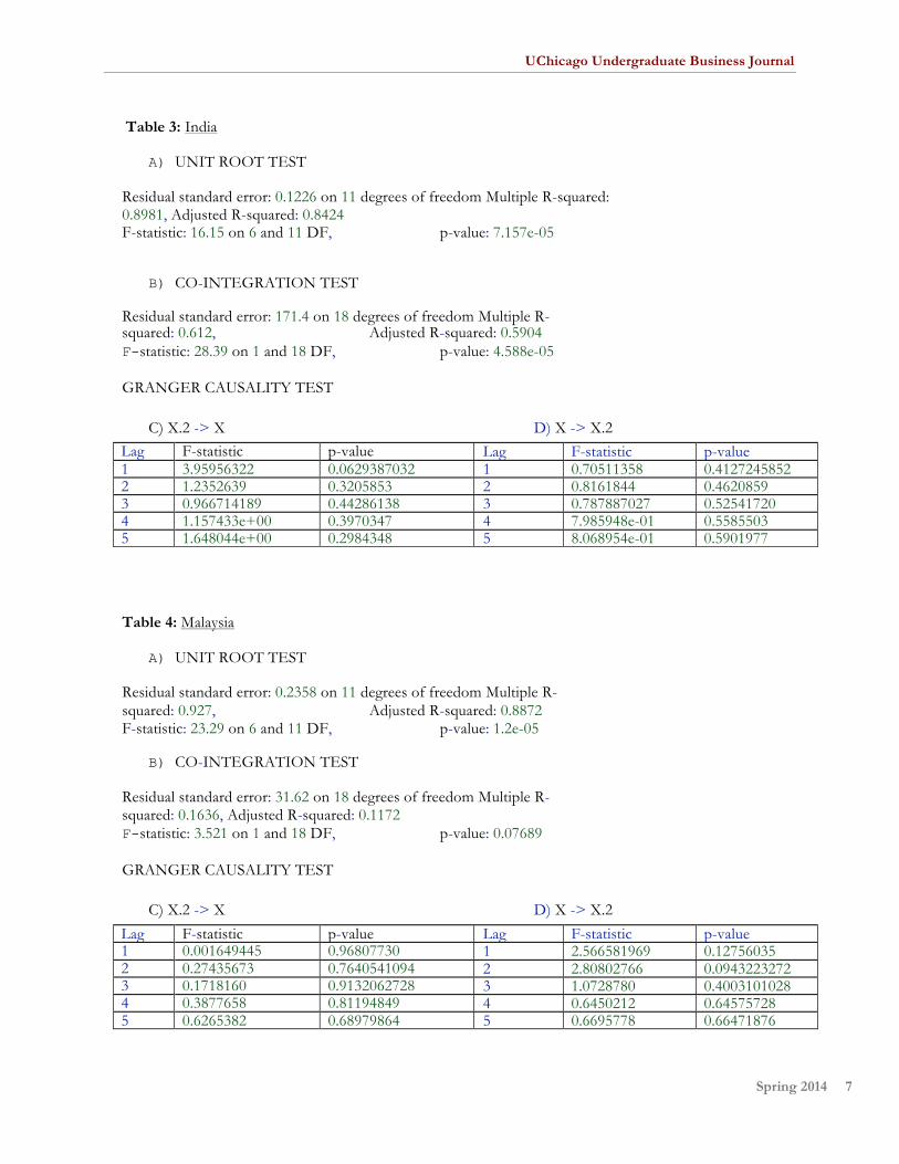
Table 3: India

A) UNIT ROOT TEST





C) X.2 -> X D) X -> X.2 Lag F-statistic p-value Lag F-statistic p-value 1 3.95956322 0.0629387032 1 0.70511358 0.4127245852 2 1.2352639 0.3205853 2 0.8161844 0.4620859 3 0.966714189 0.44286138 3 0.787887027 0.52541720 4 1.157433e+00 0.3970347 4 7.985948e-01 0.5585503 5 1.648044e+00 0.2984348 5 8.068954e-01 0.5901977

Table 4: Malaysia

A) UNIT ROOT TEST



Residual standard error: 31.62 on 18 degrees of freedom Multiple R-squared: 0.1636, Adjusted R-squared: 0.1172 F- statistic: 3.521 on 1 and 18 DF, p-value: 0.07689


C) X.2 -> X D) X -> X.2 Lag F-statistic p-value Lag F-statistic p-value 1 0.001649445 0.96807730 1 2.566581969 0.12756035 2 0.27435673 0.7640541094 2 2.80802766 0.0943223272 3 0.1718160 0.9132062728 3 1.0728780 0.4003101028 4 0.3877658 0.81194849 4 0.6450212 0.64575728 5 0.6265382 0.68979864 5 0.6695778 0.66471876


Spring 2014 8

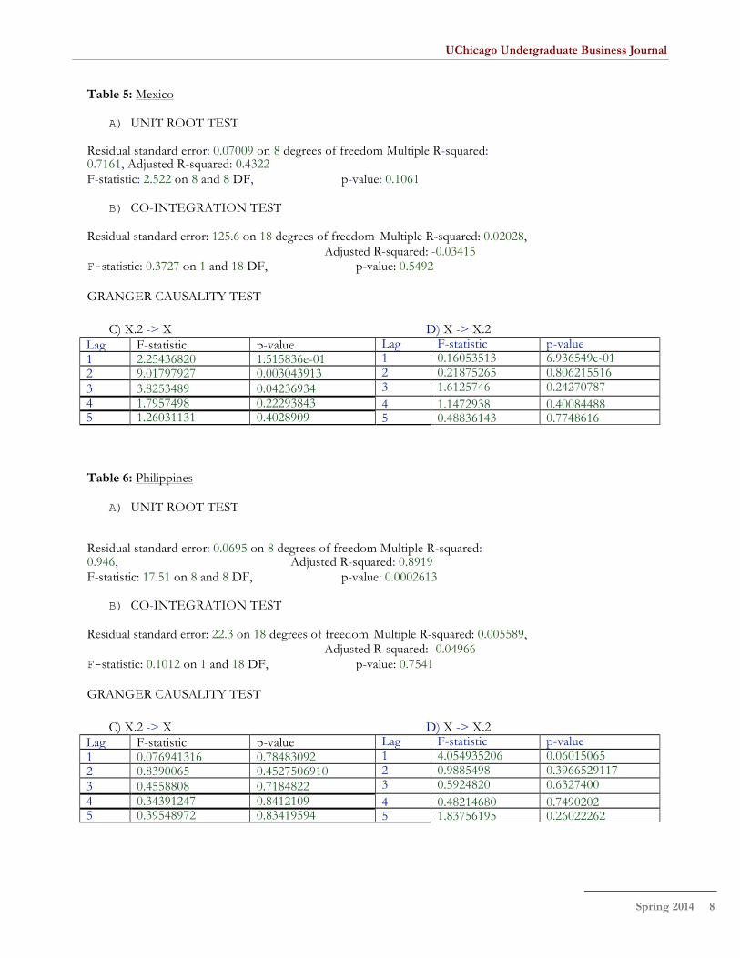
Table 5: Mexico

A) UNIT ROOT TEST

Residual standard error: 0.07009 on 8 degrees of freedom Multiple R-squared: 0.7161, Adjusted R-squared: 0.4322 F-statistic: 2.522 on 8 and 8 DF, p-value: 0.1061


Residual standard error: 125.6 on 18 degrees of freedom Multiple R-squared: 0.02028, Adjusted R-squared: -0.03415 F- statistic: 0.3727 on 1 and 18 DF, p-value: 0.5492


C) X.2 -> X D) X -> X.2 Lag F-statistic p-value Lag F-statistic p-value 1 2.25436820 1.515836e-01 1 0.16053513 6.936549e-01 2 9.01797927 0.003043913 2 0.21875265 0.806215516 3 3.8253489 0.04236934 3 1.6125746 0.24270787 4 1.7957498 0.22293843 4 1.1472938 0.40084488 5 1.26031131 0.4028909 5 0.48836143 0.7748616

Table 6: Philippines

A) UNIT ROOT TEST





C) X.2 -> X D) X -> X.2 Lag F-statistic p-value Lag F-statistic p-value 1 0.076941316 0.78483092 1 4.054935206 0.06015065 2 0.8390065 0.4527506910 2 0.9885498 0.3966529117 3 0.4558808 0.7184822 3 0.5924820 0.6327400 4 0.34391247 0.8412109 4 0.48214680 0.7490202 5 0.39548972 0.83419594 5 1.83756195 0.26022262


Spring 2014 9

Table 7: South Africa

A) UNIT ROOT TEST





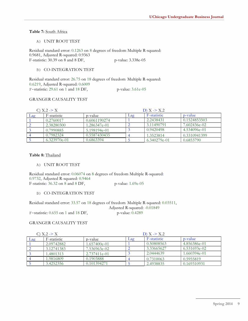
C) X.2 -> X D) X -> X.2 Lag F-statistic p-value Lag F-statistic p-value 1 0.2760017 0.6061190274 1 2.2438431 0.1524853503 2 2.38280300 1.286347e-01 2 3.11490791 7.602436e-02 3 0.7990885 5.198194e-01 3 0.9420498 4.534096e-01 4 0.7982324 0.5587430435 4 1.3523814 0.3310941399 5 6.323970e-01 0.6863394 5 6.340279e-01 0.6853790

Table 8: Thailand

A) UNIT ROOT TEST





C) X.2 -> X D) X -> X.2 Lag F-statistic p-value Lag F-statistic p-value 1 2.09742882 1.657400e-01 1 0.50808563 4.856386e-01 2 3.12741383 7.536963e-02 2 3.33665627 6.531693e-02 3 1.4801313 2.737411e-01 3 2.0444639 1.660394e-01 4 1.9816809 0.1903888 4 0.7310063 0.5955819 5 3.4252356 0.101394271 5 2.4938835 0.169310931


Spring 2014 10

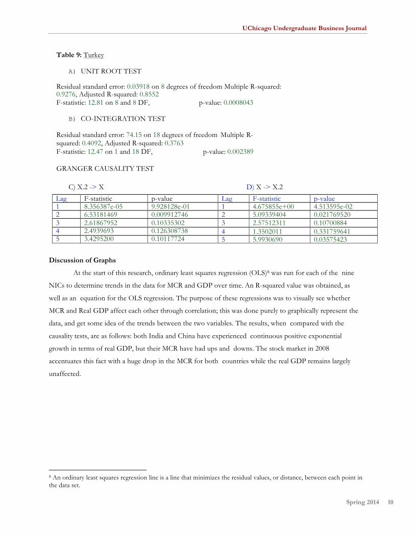
Table 9: Turkey

A) UNIT ROOT TEST





C) X.2 -> X D) X -> X.2

Lag F-statistic p-value Lag F-statistic p-value 1 8.356387e-05 9.928128e-01 1 4.675855e+00 4.513595e-02 2 6.53181469 0.009912746 2 5.09339404 0.021769520 3 2.61867952 0.10335302 3 2.57512311 0.10700884 4 2.4939693 0.126308738 4 1.3502011 0.331759641 5 3.4295200 0.10117724 5 5.9930690 0.03575423

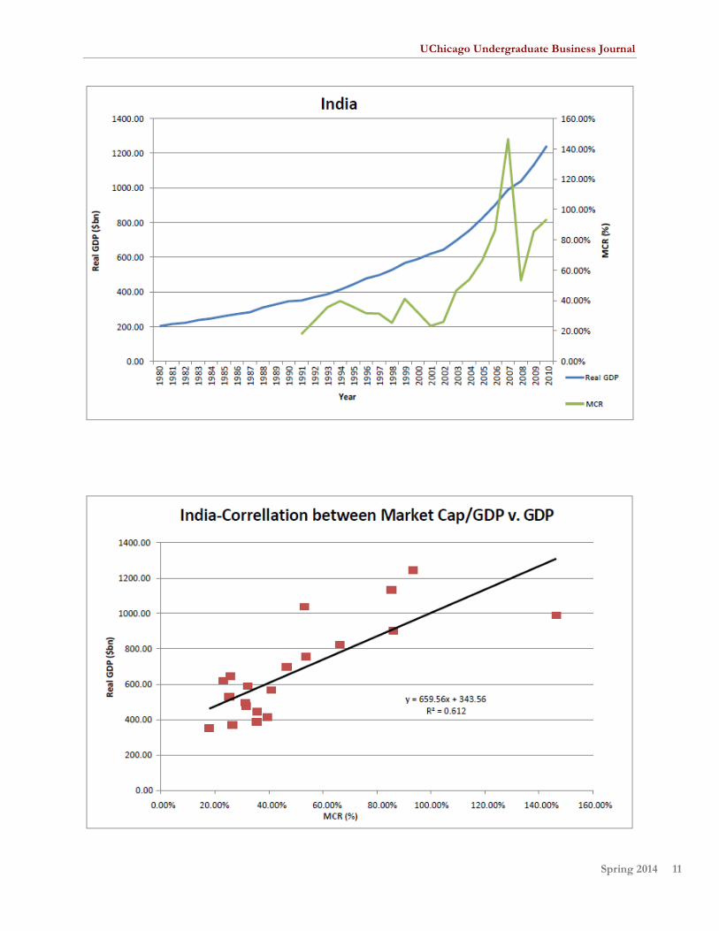
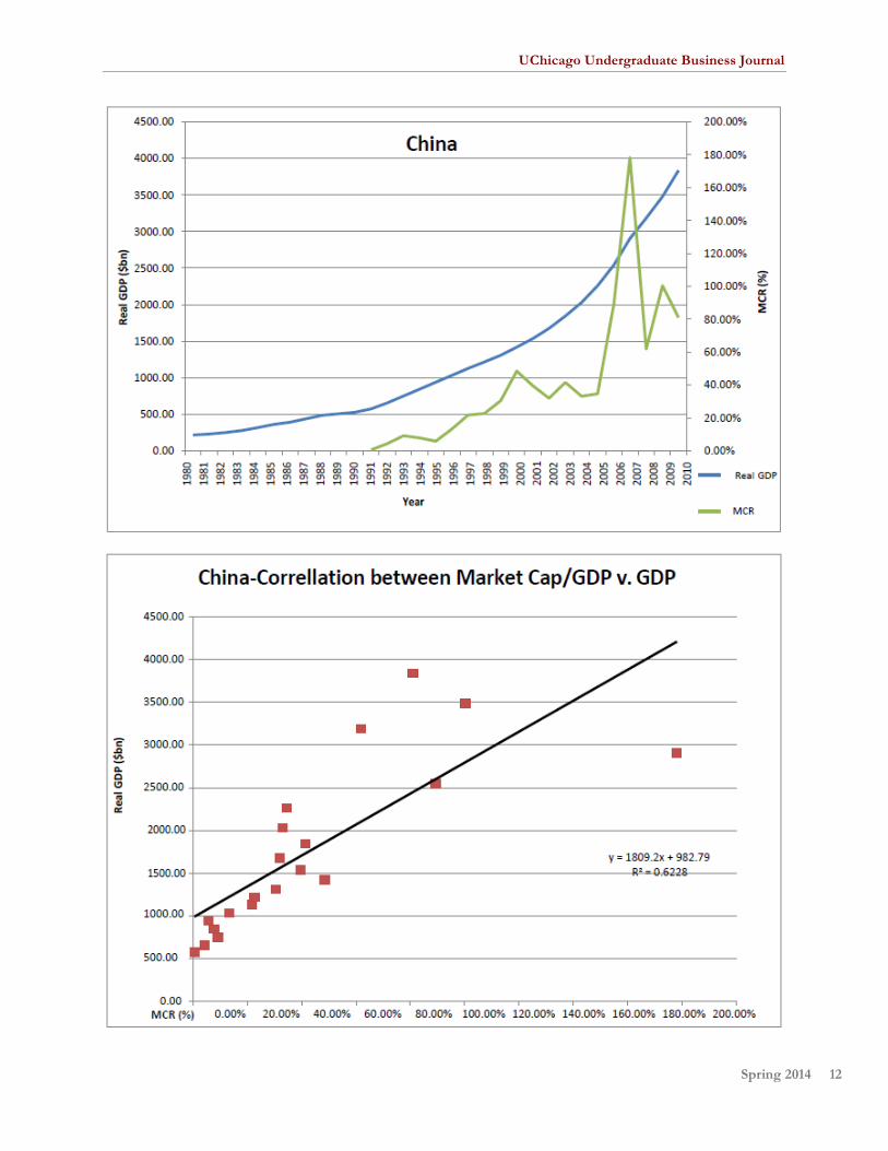
Discussion of Graphs

At the start of this research, ordinary least squares regression (OLS)8 was run for each of the nine

NICs to determine trends in the data for MCR and GDP over time. An R-squared value was obtained, as

well as an equation for the OLS regression. The purpose of these regressions was to visually see whether

MCR and Real GDP affect each other through correlation; this was done purely to graphically represent the

data, and get some idea of the trends between the two variables. The results, when compared with the

causality tests, are as follows: both India and China have experienced continuous positive exponential

growth in terms of real GDP, but their MCR have had ups and downs. The stock market in 2008

accentuates this fact with a huge drop in the MCR for both countries while the real GDP remains largely

unaffected.

8 An ordinary least squares regression line is a line that minimizes the residual values, or distance, between each point in the data set.


Spring 2014 11


Spring 2014 12


Spring 2014 13

Discussion

There are three tests that were conducted in this project: an augmented Dickey- Fuller unit root test

(ADF), an Engle and Granger Co-integration test (Engle test), and a Granger Causality Test. The former two

tests are required in order to test whether the variables are stationary and then, if not, to check if they are at

least co-integrated. As per the results, the variables were stationary for eight of nine countries, Mexico being

the odd one out. The importance of stationary variables is significant. It indicates the variables have a

constant unconditional mean and variance that do not change over time for the Granger Causality test. A

common example of something stationary is white noise because it has a constant, flat power spectral density.

Since Mexico has a unit root test, a co-integration test is required to find if the variables are at least co-

integrated.

Two or more time series are co-integrated if they share a common stochastic process9.. Previously, it

was determined that one cannot use a linear regression on non-stationary time series data because it is not

accurate and will lead to spurious correlation. In 1969, Cliver Granger disproved this theory and proposed his

own test: The Granger Causality Test. Within the means of this test, he showed a way to convert non-

stationary variables to become stationary. To convert non-stationary data to become stationary, the variables

must be appropriately differenced10. This is when the Engle test is used (C.W.J. Granger, 1988). A non-

stationary variable is said to be integrated of order “a” if it is stationary after differencing “a” times11. All the

countries reject the null for the Engle test except for Mexico, Philippines, and Thailand. Since Philippines and

Thailand have stationary variables, they can still produce reliable results. As for Mexico, since it has a unit root

and fails to be co-integrated, the results in this report for Mexico are not accurate. Unfortunately, lack of

available resources precludes further tests from being conducted to make the data stationary.

Once the data was stationary, a Granger Causality Test could be conducted. The goal of this report

was to find whether uni or bi-directional causality exists between MCR and GDP. The results suggest bi-

directional causality for China, Thailand and Turkey between GDP and real market capitalization ratio at

different lag lengths and significance levels. Uni-directional causality for MCR to GDP exists for India (10% at

1 lag) and Mexico (1% at 2 lags). Uni-directional causality for GDP to MCR exists for Malaysia (10% at 2 lags),

Philippines (10% at 1 lag) and South Africa (10% at 2 lags). No causality is determined for Brazil.

Cooray in 2010 concluded that the existence of a liquid securities market promotes economic growth

when using market capitalization as a proxy for the stock market. This conclusion is in line with those of

Levine and Zervos (1996), Atje and Javanovic (1993) and Roussea (2000). The implications of this would

9 A stochastic process is the evolution of a random variable over time, and the drift rate is the rate at which the average value changes. 10 Differencing a data set involves transforming the data into a series of period-to-period differences. If the statistics of the changes in the series between periods or between seasons are constant, then the data is stationary. 11 When differencing data, there are different numbers of times you can difference the data. For example, the first difference is the series of changes from one period to the next. If Y(t) denotes the value of the time series Y at period t, then the first difference of Y at period t is equal to Y(t)-Y(t-1).


Spring 2014 14

mean that countries should implement policies to create a larger, liquid and more active stock market. This

would result in greater risk diversification and lower capital costs (Cooray 2010).

In a similar study by Mukherjee and Deb, the causal relationship between stock market development

and economic growth is examined for the Indian economy (Deb 2008). In this study, bi-directional causality

was found between MCR and GDP growth rate for India at the 1% significance level in the time period

1997-2007. This report extends this study to encompass two decades (1990-2010) as well as eight more

countries. These countries were selectively chosen in 2011 since they were part of the Newly Industrialized

Countries group.

Conclusion and Future Work

This study makes an effort to find a causal relationship between stock market development and

economic growth for the nine NICs from 1990:Q1-2010:Q1. The study was based off two questions: whether

a causal relationship exists and, if so, what is the nature/direction of it? 2005 nominal GDP values are used as

a proxy for economic growth. There are three main indicators for economic growth: real market capitalization

ratio, real value traded ratio, and stock market volatility. This study focuses on real market capitalization ratio.

Results for eight of the nine countries can be deemed accurate, since Mexico failed to have stationary

variables and the variables are not differenced to become stationary in this present study. Of the eight

countries, only one, Brazil, was found not to have any form of causality. Bi-directional causality is found for

China, Thailand and Turkey. Uni-directional causality for MCR to GDP is found for India and Mexico, and

uni-directional causality for GDP to MCR is found for Malaysia, Philippines, and South Africa. The “supply

leading” hypothesis, which claims a causal relationship between financial development and economic growth,

is found to hold true for China, India, Turkey and Thailand for the given time period (Deb 2008). The

hypothesis states that the intentional development of financial institutions and markets would increase the

supply of financial services and thus lead to economic growth (Deb 2008). The governments of these

countries should direct fiscal and monetary policies towards the financial institutions and promote the growth

of the financial sector.

As for future research, a similar study can be conducted for developed countries in the world, such as

the United States, France, Germany and Japan, and contrast the results with the results of this study. Volumes

of literature have stated that stock market development does not influence economic growth in developing

countries; rather it influences economic growth in developed countries (Demetrides 1996).

Due to time constraints, a few things could not be done in this study. Firstly, converting Mexico’s

variables into stationary variables through the co-integration test would have yielded more reliable results for

Mexico. In addition, as a disclaimer, several crux issues for the Granger Causality Test have been highlighted

in recent studies on time-series econometrics (Deb 2008). Most importantly, the causality test is highly

influenced by lag length. Therefore, if the chosen lag length is smaller than the true lag length, the omission of


Spring 2014 15

relevant lags may cause bias. In addition, the Granger Causality test is based on the assumption that there are

no other outside variables that can influence the causality.

Misleading results may be produced if the relationship truly involves three or more variables, since

the causality test is designed to handle variables in pairs. A much stronger statistical test is the vector auto-

regression (VAR). The VAR is much more robust against lag length and does not require a unit root test and

co-integration test. The VAR is a statistical model that captures the linear interdependencies among multiple

time series and was first proposed by Toda and Yamamoto in 1995. The test is similar to the Granger

Causality test but augmented with extra lags depending on the maximum order of integration of the time

series under consideration. For future research, a VAR can produce more reliable and stronger results.

Following the conclusion of this research, evidence has shown that the stock market does play a

cardinal role in the economy, and it should thus be the target of much government discussion and policies. It

is important to note that stock market development causing economic growth is very country-specific. A

general statement cannot be made saying stock market development causes economic growth. Economic

growth relies heavily on a country’s specific financial institution and government policies. We ust keep this in

mind when assessing causes of economic growth


Bibliography

Arestis, P., Demtriades, P., & Luintel K. (2001). Financial Development and Economic

Growth: The role of stock markets. Journal of Money, Credit and Banking, 33, 16-41.

Atje, R., & Javanovic B. (1993). Stock Markets and Development. European Economic Review,

37, 632-640.

Caporale, M., Guglielmo (2001). Stock Market Development and Economic Growth: The causal

linkage. Journal of Economic Development, Vol. 29.

Cooray, Arusha (2010). Do Stock Markets Lead to Economic Growth? Journal of Policy

Modeling, 448-460.

C.W.J. Granger (1988), Some Recent Development in a Concept of Causality, Journal of

Econometrics, Volume 39, Issues 1–2, September–October 1988, Pages 199-211.

Dawson, P.J. (2008). Financial Development and Economic Growth in Developing Countries.

Progress in Development Studies, 325-31.

Deb, G., Soumya, & Mukherjee, Jaydeep (2008). Does Stock Market Development Cause

Economic Growth? A Time Series Analysis for Indian Economy. International Research Journal of

Finance and Economics, Issue 21.

Demetrides, O., Panicos, Hussein, A., Khaled (1996). Does Financial Development Cause

Economic Growth? Time-series Evidence from 16 countries. Journal of Development Economics, 387-

411.

Devereux, M., & Smith, G. (1994). International Risk Sharing and Economic Growth.

International Economic Review, 35, 535-550.

Dicle, F., Mehmet, Beyhan, Aydin (2010). Market Efficiency and International Diversification:

Evidence from India. Elsevier, 313-339.

Durham, J., Benson (2002). The effects of stock market development on growth and private

investment in lower-income countries. Emerging Markets Review, 211-232.

Filer, K., Randall, Hanousek, Jan, & Campos, F., Nauro (1999). Do Stock Markets Promote

Economic Growth? Financial Economics, 267.

Levine, Ross, & Zervos, Sara (1998). Capital Control Liberalization and Stock Market

Development. World Development, 1169-1183.

Levine, Ross, & Zervos, Sara (1998). Stock Markets, Banks, and Economic Growth. The

American Economic Review, Vol. 88, No. 3 537-558.

Pal, Parthapratim (2006). Foreign Portfolio Investment, Stock Market and Economic

Development: A Case Study of India. Promoting Development in a Globalized World.

Patrick, T., Hugh (2005). Financial Development and Economic Growth in Underdeveloped

Countries. Economic Development and Cultural Change, 174-189.


Rousseau, P., & Wachtel, P. (2000). Equity markets and growth: Cross-country evidence on

timing and outcomes, 1980-1995. Journal of Banking and Finance, 24, 1933-1957.

Rajan, RG. (2010). Fault lines. Princeton, NJ: Princeton University Press.

Singh, A. (1997). Financial Liberalisation, Stock Markets and Economic Development. Economic

Journal, 107, 771-782.

Toda, Y., Hiro, Yamamoto, Taku (1996). Statistical Inference in Vector Autoregressions with

Possibly Integrated Processes. Journal of Econometrics, 225-250.

mittal effects of market capitalization ratio on gdp ... gdp growth and capital market robustness in...

Documents