mit - center for real estate center for real estate - …...a real options analysis of a vertically...
TRANSCRIPT

A Real Options Analysis of a Vertically Expandable Real Estate Development
by
Anthony C. Guma
Bachelor of Design in Architecture, University of Florida, 1998
Master of Architecture, Massachusetts Institute of Technology, 2001
Submitted to the Department of Urban Studies and Planning in Partial Fulfillment of the Requirements for the Degree of
Master of Science in Real Estate Development
at the
Massachusetts Institute of Technology
September, 2008
©2008 Anthony C. Guma All rights reserved.
The author hereby grants to MIT permission to reproduce and to distribute publicly paper and electronic copies of this thesis document in whole or in part in any medium now known or
hereafter created. Signature of Author______________________________________________________________
Department of Urban Studies and Planning July 31, 2008
Certified by____________________________________________________________________
Richard de Neufville Professor of Engineering Systems and of Civil and Environmental Engineering
Thesis Supervisor Accepted by____________________________________________________________________
Brian A. Ciochetti Chairman, Interdepartmental Degree Program in
Real Estate Development

2

3
A Real Options Analysis of a Vertically Expandable Real Estate Development
by
Anthony C. Guma
Submitted to the Department of Urban Studies and Planning
on July 31, 2008 in Partial Fulfillment of the Requirements for the Degree of
Master of Science in Real Estate Development Abstract Like many great business ventures, grand successes in real estate development are often attributed to individuals with strong visions and talent, as well as a keen foresight on the future conditions which will ultimately decide the value of their projects. Even with the best forecasts and predictions, this type of a clear view of the future real estate market is typically difficult to bring into focus. By considering developments which provide the ability to react accordingly to the uncertainty of future forces, developers can better manage the risk associated with a potential weak market while also gaining the potential to benefit in a strong one. Flexibility of this type in real estate is generally known as a “real option.” Even in dense urban centers with a limited amount of developable land, market uncertainty may still exist. Therefore, flexibility in that type of environment could allow a developer to be better positioned should a market improve or decline. One way to provide this type of flexibility on urban sites is to develop a given quantity of space initially with the option to add more vertically in the future. Although rare, such vertical expansions are quite feasible and the real option is quantifiable. This thesis investigates the value of providing a real option to vertically expand a structure in the future. Real option valuation is often regarded as a complex procedure and outside of typical real estate finance. This investigation will adopt a previously developed methodology based on familiar spreadsheet techniques and common valuation metrics such as net present value. To explore the use of this methodology and the potential value of vertical expansion, the Health Care Service Corporation headquarters in Chicago, IL is the basis of an analysis. This structure represents an existing building with the built-in option to expand vertically to almost twice its initial height. Thesis Supervisor: Richard de Neufville Title: Professor of Engineering Systems and of Civil and Environmental Engineering

4
Acknowledgements I would like to sincerely thank Professor Richard de Neufville for his guidance, insight, and
dedication as the supervisor of this thesis. From the very beginning, his comments and
enthusiasm were an inspiration to this work and his vast experience always provided the
clearest advice. It was a pleasure to conduct this work as an interdisciplinary link between
the Center for Real Estate and the Engineering Systems Division at MIT.
Professor David Geltner was essential to the success of this thesis. I am very thankful for his
support along the way, his patience in working through the stumbling points with me, and for
his introduction to Professor de Neufville. This thesis would not have existed without his
discovery of the HCSC project and his help in developing a relationship with the team in
Chicago. Also, his dedication to instructing finance at the CRE is unwavering and he was a
valuable part of my experience over the past year.
Michel-Alexandre Cardin was an excellent resource for all aspects of this research. His
lecture on flexibility and tutorial of the engineering-based methodology was a strong factor in
cementing my interest in this topic.
Many thanks go to the HCSC Vertical Completion project team in Chicago for being terrific
hosts, providing great information, and allowing us to share in a truly amazing project.
I would like thank my all of my fellow classmates, the faculty, and staff of the CRE for
making this year such a great experience. Especially to Jason Pearson and Kate Wittels, two
classmates who explored this fascinating topic and the HCSC project along with me.
To all of my great friends, thank you for being around when I needed distractions the most.
Especially those who I neglected so often over the year.
Finally, I am utterly grateful to have the best parents and family imaginable and who always
give me their unconditional support in so many ways... Over this year, and in all of my
endeavors.

5
Table of Contents Abstract.....................................................................................................................................3
Acknowledgements...................................................................................................................4
Table of Contents.....................................................................................................................5
List of Figures...........................................................................................................................7
List of Tables............................................................................................................................9
Chapter 1: Introduction........................................................................................................11
1.1 Background............................................................................................................11
1.2 Methodology..........................................................................................................12
1.3 Objective................................................................................................................13
Chapter 2: Real Options Overview................................................................................14
2.1 Description of Real Options..................................................................................14
2.2 Real Option Types.................................................................................................15
2.3 Real Option Valuation Methods............................................................................16
2.3.1 Real Options in Relation to Financial Options......................................17
2.3.2 Real Options Analysis in Real Estate.....................................................19
2.3.3 The “Engineering-Based” Approach to Real Option Valuation............25
2.4 Relevant Background Research on Real Options..................................................27
2.4.1 Industry Perceptions...............................................................................27
2.4.2 Economics-Based Approach and Engineering-Based Approach
Compared........................................................................................................28
Chapter 3: HCSC Headquarters....................................................................................30
3.1 Project Description................................................................................................30
3.1.1 History....................................................................................................30
3.1.2 Site Characteristics.................................................................................32
3.1.3 Vertical Expansion Decision..................................................................34
3.2 Project Timeline Summary....................................................................................36
3.3 Building Specifications..........................................................................................37
3.4 Real Options “in” Projects.....................................................................................38
6
3.4.1 Real Options “in” Real Estate Developments and the HCSC
Tower..............................................................................................................39
Chapter 4: Real Options Analysis of the HCSC Headquarters...................................45
4.1 Methodology..........................................................................................................45
4.2 Assumptions………………..................................................................................46
4.3 Uncertain Variables and Decision Rules...............................................................47
4.3.1 Projected Rent........................................................................................47
4.3.2 Lease-Up Simulation..............................................................................49
4.2.3 Option Decision Rule.............................................................................50
4.4 Simulation and Scenario Comparison...................................................................54
4.5 Analysis Observations...........................................................................................59
Chapter 5: Conclusion.........................................................................................................62
Bibliography..........................................................................................................................64
Worked Cited...............................................................................................................64
Additional Reading......................................................................................................65
Interviews Conducted..................................................................................................66
Appendix...........................................................................................................................67

7
List of Figures Figure 1.1: HCSC headquarters with vertical expansion / completion seen under
construction, 2008 (Source: Author)...........................................................................13
Figure 2.1: Comparison of NPV and Real Option Methodologies (Source:
Adopted from Leslie and Michaels, 1997)..................................................................15
Figure 2.2: Mapping an Investment Opportunity onto a Call Option (Source:
Luehrman, T. A., 1998)...............................................................................................18
Figure 2.3: One Year Monthly Binomial Value Tree (Source: Adopted from
Geltner et al, 2007)......................................................................................................21
Figure 2.4: One Year Value Probabilities (Source: Adopted from Geltner et al,
2007)............................................................................................................................22
Figure 2.5: Land Value as a Function of Current Built Property Value (Source:
Adopted from Geltner et al, 2007)...............................................................................24
Figure 2.6: Merits and demerits of the economics-based approach and the
engineering-based approach (Source: Masunaga, 2007).............................................28
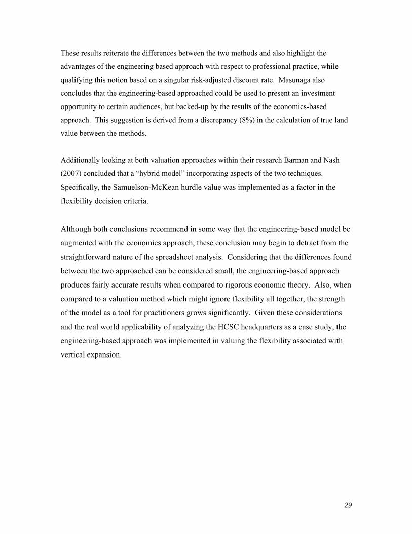
Figure 3.1: Comparison of the typical speculative office building characteristics
with the requirements of HCSC (BCBS) (Source: Goettsch Partners,
2008)............................................................................................................................32
Figure 3.3: Project location plan, structure circled (Source: Goettsch Partners,
2008)............................................................................................................................33
Figure 3.4: Former rail yard at site location (Source: Goettsch Partners, 2008).....................34
Figure 3.5: Land cost with respect to vertical or horizontal expansion options.
Note: Actual dollar amount were redacted (Source: Goettsch Partners,
2008)............................................................................................................................36
Figure 3.6: Site Plan (Source: Goettsch Partners, 2008)..........................................................37
Figure 3.7: Architect’s renderings of Phase 1 and Phase 2 (Source: Goettsch
Partners, 2008).............................................................................................................38
Figure 3.8: Comparison between real options “on” and “in” projects (Source:
Wang and de Neufville, 2005).....................................................................................39

8
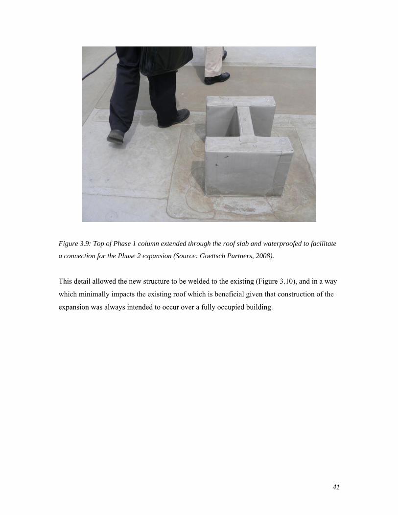
Figure 3.9: Top of Phase 1 column extended through the roof slab and
waterproofed to facilitate a connection for the Phase 2 expansion
(Source: Goettsch Partners, 2008)...............................................................................41
Figure 3.10: Welded connection of the new and existing structure at the
Phase 1 roof level (Source: Author)............................................................................42
Figure 3.11: Typical floor place with Phase 1 and Phase 2 elevator arrangement
indicated (Source: Goettsch Partners, 2008)...............................................................43
Figure 3.12: Phase 1 atrium and Phase 2 elevators under construction in
provided space (Source: Goettsch Partners, 2008)......................................................44
Figure 4.1: Example of possible achieved rent........................................................................49
Figure 4.2: Example of a possible lease-up scenario...............................................................50
Figure 4.3: Decision rule diagram............................................................................................51
Figure 4.4: Example of a possible lease-up scenario. (A) Lease-up rate.
(B) Cumulative total lease-up and lease-up per Phase................................................53
Figure 4.5: VARG (Value At Risk or Gain) curves base in the analysis results.....................58
Figure 4.6: Expected NPV as a function of the price of flexibility..........................................60
9
List of Tables Table 2.1: Option Premium Value Due to Future Uncertainty in Built
Property Value (Source: Adopted from Geltner et al, 2007).......................................20
Table 2.2: Samuelson-McKean formula variables...................................................................23
Table 3.1: Building space characteristics (Source: Goettsch Partners, 2008)..........................37
Table 4.1: Simplified building program for analytical purposes.............................................46
Table 4.2: Decision rule and determination of exercise year...................................................54
Table 4.3: Development characteristics and costs for analysis................................................55
Table 4.4: Simulation decision.................................................................................................56
Table 4.5: Analysis results.......................................................................................................56
Table 4.6: Analysis results with 20% pre-leasing hurdle.........................................................60
Table 4.7: Analysis results with 90% pre-leasing hurdle.........................................................61
Table A.1: Property and cost inputs.........................................................................................67
Table A.2: Other costs and relevant rates................................................................................67
Table A.3: Rent growth simulation..........................................................................................68
Table A.4: Lease-up simulation...............................................................................................69
Table A.5: Phase 1 valuation...................................................................................................70
Table A.6: Phase 1+2 valuation...............................................................................................71
Table A.7: Flexible case valuation...........................................................................................72

10
11
Chapter 1: Introduction
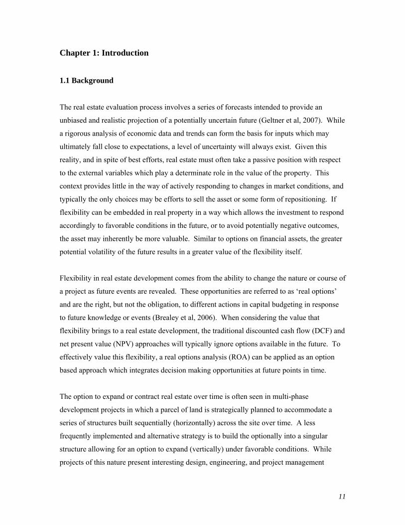
1.1 Background
The real estate evaluation process involves a series of forecasts intended to provide an
unbiased and realistic projection of a potentially uncertain future (Geltner et al, 2007). While
a rigorous analysis of economic data and trends can form the basis for inputs which may
ultimately fall close to expectations, a level of uncertainty will always exist. Given this
reality, and in spite of best efforts, real estate must often take a passive position with respect
to the external variables which play a determinate role in the value of the property. This
context provides little in the way of actively responding to changes in market conditions, and
typically the only choices may be efforts to sell the asset or some form of repositioning. If
flexibility can be embedded in real property in a way which allows the investment to respond
accordingly to favorable conditions in the future, or to avoid potentially negative outcomes,
the asset may inherently be more valuable. Similar to options on financial assets, the greater
potential volatility of the future results in a greater value of the flexibility itself.
Flexibility in real estate development comes from the ability to change the nature or course of
a project as future events are revealed. These opportunities are referred to as ‘real options’
and are the right, but not the obligation, to different actions in capital budgeting in response
to future knowledge or events (Brealey et al, 2006). When considering the value that
flexibility brings to a real estate development, the traditional discounted cash flow (DCF) and
net present value (NPV) approaches will typically ignore options available in the future. To
effectively value this flexibility, a real options analysis (ROA) can be applied as an option
based approach which integrates decision making opportunities at future points in time.
The option to expand or contract real estate over time is often seen in multi-phase
development projects in which a parcel of land is strategically planned to accommodate a
series of structures built sequentially (horizontally) across the site over time. A less
frequently implemented and alternative strategy is to build the optionally into a singular
structure allowing for an option to expand (vertically) under favorable conditions. While
projects of this nature present interesting design, engineering, and project management
12
challenges, the result of these efforts is a clear option in the scheme which may ultimately
add the value of flexibility to developments which ordinarily stand statically.
This thesis analyzes and evaluates a real estate development project with this type of
embedded vertical expansion flexibility. Specifically, this study is based on a downtown
Chicago commercial office tower with the built-in option to expand vertically to almost twice
its initial height. Through the use of a real options analysis, the value of the optional future
investment opportunity will be determined and compared to inflexible base case scenarios.
1.2 Methodology
There are many documented real option valuation methodologies which range in levels of
complexity and are demonstrated on a varied set of applications. The valuation model used
in this thesis is based the notion that the application of an ROA to investment decisions can
be most effective in the hands of managers in a way that limits the calculation complexities
that are generally associated with the valuation of real options (Leslie and Michaels, 1997;
Copland and Antikarov, 2001). Therefore, the valuation methodology applied in this thesis is
an application of the simple spreadsheet analysis described by de Neufville et al (2006), and
also referred to as an engineering-based approach. This approach uses Monte Carlo
simulation techniques within Excel® to simulate possible future outcomes as a way to
determine expected net present values (ENPV).
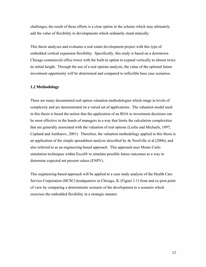
This engineering-based approach will be applied to a case study analysis of the Health Care
Service Corporation (HCSC) headquarters in Chicago, IL (Figure 1.1) from and ex-post point
of view by comparing a deterministic scenario of the development to a scenario which
exercises the embedded flexibility in a strategic manner.

13
Figure 1.1: HCSC headquarters with vertical expansion / completion seen under construction,
2008 (Source: Author).
1.3 Objective
In applying the engineering-based valuation method to the HSCS headquarters, a current
project with built-in flexibility, the objective of this thesis is to investigate the following:
o The reasons why a real options analysis is appropriate for a development project such
the HCSC tower.
o The characteristics of a real estate development which make vertical expansion
desirable and feasible.
o A real options analysis to determine the potential value of the flexibility in a
vertically phased structure.

14
Chapter 2: Real Options Overview
The basic toolset at work when valuing a real estate development project includes a multi-
year discounted cash flow analysis and decision based on a net present value. The NPV rule
is commonly understood to provide a sound method for deciding between mutually exclusive
opportunities by identifying the alternative with the greatest value. This method also allows
for the rejection of any alternative which presents a negative NPV. This process inherently
forces a decision based on a set of fixed forward looking assumptions and ignores the value
achievable when flexibility is provided in a project. Real options analysis provides a means
to quantity the value which flexibility brings to a project in its ability to respond
appropriately to uncertainties in the future real estate market.
The concept of a real option is very broad and considerable information is available within
financial literature describing various definitions, valuation methods, and applications. The
underlying theories and applications are far reaching, and it is beyond the scope of this thesis
to provide a comprehensive description of real options in a general way. It is the intent of
this chapter to describe the basic concepts as they relate to real estate and in particular to the
analysis of a vertically phased development project. This chapter also provides background
and precedent information which positions the work within the greater literarily discourse on
flexibility and real options in real estate.
2.1 Description of Real Options
In a simplified sense, a real option in real estate is the opportunity to make changes to a
development project or other investment as previously unknown information is revealed.
Different sources on the topic of real options all have slightly different definitions although
the general sentiment is consistent. Also, in contrast to financial options in which value is
derived from an underlying financial asset, real options derive their values from a tangible or
real asset. A more formal definition relevant to the context of this study is that a “real option
is the right, but not the obligation, to take an action (e.g., deferring, expanding, contracting,
or abandoning) at a predetermined cost called the exercise price, for a predetermined period
of time – the life of the option (Copland and Antikarov, 2001, p.5).” In all cases, the

15
motivating factor in the decision making process is it to take advantage of a potential future
upside to an investment, and to limit a potential downside. These characteristics of real
options provide the benefit from flexibility in responding to the future uncertainties for which
traditional underwriting and DCF analysis attempts to account for. Although the depicted
real option model is not directly implemented in this thesis, Figure 2.1 represents a
comparison between a traditional NPV analysis and an ROA.
Figure 2.1: Comparison of NPV and Real Option Methodologies (Source: Adopted from Leslie and Michaels, 1997).
2.2 Real Option Types
While financial options generally provide the owner with the option to buy (a call option) or
sell (a put option) an underlying asset at a specified price (exercise or strike price) for a
specified amount of time, real options provide flexibility in several analogous ways. The
general types of real options which are applicable to real estate development may be
summarized in the following list:
o A deferral option – the right to delay a project.
o An abandonment option – the right to terminate a project.
o An option to expand/contract – the right to increase or decrease the scale of a
development.
o A switching option – the right to change from one product type to another.

16
o A growth option – an option acquired through investing in the creation of future
growth opportunities (e.g. new technologies or infrastructure).
o A compound option – a phased option in which an option is contingent on the prior
exercise of a preceding option (an option on an option).
Based on a list defined by Brach (2003).
Given the focus of this study on a vertically phased development project, the compound
option is the primary type investigated. As described in greater detail subsequently, the
option to construct an additional series of levels above an existing building is contingent of
the prior decision to exercise the initial option to develop the land originally.
2.3 Real Option Valuation Methods
Much has been written with regard to the shortcomings of DCF/NPV techniques when
compared to real options analyses. This criticism is based on these models being unable to
account for potential flexibility at the time of the investment decision. When the decision to
invest is made irreversibly and without flexibility, the ability to react to the arrival of new
information at a later date is lost. This value can been seen as an opportunity cost which is
not a considered in a traditional DCF/NPV analysis. While incorporating this opportunity
cost into the analysis can attempt to capture the value of the option, an alternative approach is
to adopt option pricing models typically used in valuing financial assets to the investment
opportunities of real assets (Dixit and Pindyck, 1994). In summary and with specific respect
to real estate, Sirmans summarized this dilemma such that a:
DCF model is not only incomplete, but may lead to costly errors. Investors must
decide when to invest, how to modify operating plans during the life of the project,
and when to sell the investment. Existing research shows the conventional DCF
techniques can be poorly suited for investment valuation in the presence of ‘real
options.’ If the NPV of a project is redefined to include the opportunity cost of
exercising the option to invest, then the standard rule of ‘invest if NPV is positive’ is
still applicable (1997, p. 95)

17
In recognition of the DCF/NPV limitations, the use of ROA has gained traction, slowly at
first, in the context of capital budgeting since the term was introduced in the late 1970’s.
From the initial academic interest in the 1980’s, the concepts and methodologies of real
options began to take a foothold a among industry professionals when considering a range of
corporate investment opportunities (Borison, 2005). Following from these beginnings, ROA
have been applied within the real estate context for topics which include the determination of
land value, the optimum time to switch from one use to another, the value of flexibility in a
multi-phase development, and many other instances.
While the use of ROA has found a place among practitioners, the methodologies for
conducting such analyses are diverse. The methods vary in complexity and range from
quantitatively rigorous models based on financial option valuation, to procedures which use
techniques and intuitions that real estate developers are familiar with. For example, although
distinct in its ability to incorporate flexibility in investment decisions, in many cases the
technical aspects of an ROA includes discounting cash flows and net present value
calculations as integrated parts of the valuation (Copland and Antikarov, 2001). So in this
sense, ROA does not act as a replacement to DCF, as a DFC analysis is often necessary to
understand the value of the underlying asset (Brealey et al, 2006). This relationship places
real options into the parlance of widely understood real estate finance (DCF analysis, NPV
rule). When combined with methods which are implemented within the familiar tool of
Excel®, ROA has the potential to augment common professional practices.
2.3.1 Real Options in Relation to Financial Options
To see the relationship between financial options and real options as well as the role of NPV
as a link to real options analyses, one way is by looking at the framework and the associated
description for “mapping the characteristics of the business opportunity onto the template of
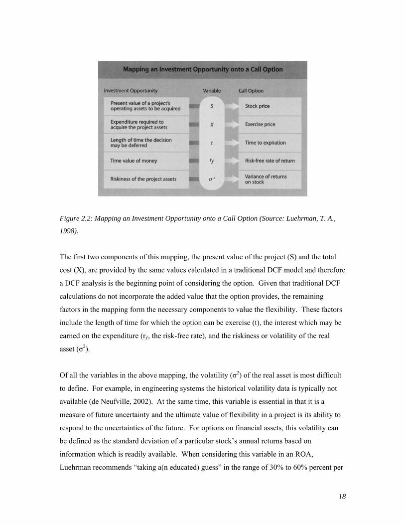
a call option” proposed by Luehrman (1998). Luehrman’s framework begins with an
identification of the option to be investigated and its properties such as expected cash flows,
length of time to options can be deferred, and the projected costs to exercise the option.
After this initial identification, the properties of the investment opportunity are then mapped
on to the analogous requirements of a European call option (Figure 2.2).
18
Figure 2.2: Mapping an Investment Opportunity onto a Call Option (Source: Luehrman, T. A.,
1998).
The first two components of this mapping, the present value of the project (S) and the total
cost (X), are provided by the same values calculated in a traditional DCF model and therefore
a DCF analysis is the beginning point of considering the option. Given that traditional DCF
calculations do not incorporate the added value that the option provides, the remaining
factors in the mapping form the necessary components to value the flexibility. These factors
include the length of time for which the option can be exercise (t), the interest which may be
earned on the expenditure (rƒ, the risk-free rate), and the riskiness or volatility of the real
asset (σ2).
Of all the variables in the above mapping, the volatility (σ2) of the real asset is most difficult
to define. For example, in engineering systems the historical volatility data is typically not
available (de Neufville, 2002). At the same time, this variable is essential in that it is a
measure of future uncertainty and the ultimate value of flexibility in a project is its ability to
respond to the uncertainties of the future. For options on financial assets, this volatility can
be defined as the standard deviation of a particular stock’s annual returns based on
information which is readily available. When considering this variable in an ROA,
Luehrman recommends “taking a(n educated) guess” in the range of 30% to 60% percent per

19
year when information is scarce, researching information on similar industries, and
simulating a distribution of returns with computer based Monte Carlo simulations. When
researching data, comparables to consider would be publicly traded stocks of businesses with
investment opportunities which would be of a similar level of risk (Brealey et al, 2006). For
real estate, the volatility of individual build properties is typically in the range of 10% to 25%
per year (Geltner et al 2007).
Following this mapping of variables, the framework continues by determining the value of
the call option through and application of the Black-Scholes formula using the mapped
variables as inputs. Luehrman goes on to present this framework for a compound option in
which the NPV of the flexible project equals the NPV of the first phase plus the value of the
call option (NPV Flexible = NPV Phase 1 + Option Value Phase 2). This is facilitated by
first separating the cash flows of the two phases and performing a DCF analysis for each.
2.3.2 Real Options Analysis in Real Estate
The preceding example describes how the valuation of real options can be understood in the
context of financial options, and how the lexicon of real options is shared with the typical
vocabulary of real estate finance. This introduction can be continued by looking at more
specific methods of using real option analyses, or more generally, option valuation theory
(OVT) in the context of real estate development. One application of this theory is the call
option model of land value and related the value of land the development option it provides
an owner (Geltner et al, 2007).
The following examples in this section summarize the examples presented by Geltner et al,
(2007). The original text should be referenced for more detailed explanations.
An example of the option valuation theory as it relates directly to land value can be seen in a
one-period binomial model of a one year deferral option to develop a structure. This model
is based on acquiring the option to develop a building immediately, or to defer the
development for one year. The following table summarizes the value of the land with the
deferral option and the value of the option (Table 2.1). The “action” row of the table can be

20
understood with a review of a typical call option which provides the owner the right, but not
the obligation to buy an underlying asset. The option has a positive value when the current
price of the underlying asset has a spot price (S) above the strike price (K), the price in which
the underlying asset can be purchased for. In this case the spot price is analogous to the
value of the developed property, and the strike price relates to the construction cost. The
payoff of the call option can be expressed as MAX[(S − K), 0], and in this was payoff
captures any potential upside and limits the downside exposure to the cost of purchasing the
option. In this example in Table 2.1, the option is “in the money” when the value of the
developed property is $113.21 and in turn, the value of the options is $23.21.
($ Millions) Today
Probability 100% 30% 70%Value of Developed Property $100.00 $78.62 $113.21 Development Cost (Excluding Land Cost)
$88.24 $90.00 $90.00
NPV of Exercise $11.76 -$11.38 $23.21 (Action) (Don’t Build) (Build)Future Values 0 $23.21
Expected Value of Built Property $100.00 (Probability x Outcome) (1.0 x 11.76)
Expected Value of Option $11.76 (Probability x Outcome) (1.0 x 11.76)
PV (Today) of Alternatives @ 20% Discount Rate
$11.76
Land Value Today = MAX(11.76, 13.54) = $13.54Option Premium = $13.54 - $11.76 = $1.78
Next Year
$16.25 (0.3 x 0) + (0.7 x 23.21)
$13.54 = (16.25/1.20)
$102.83 (0.3 x 78.62) + (0.7 x 23.21)
Table 2.1: Option Premium Value Due to Future Uncertainty in Built Property Value (Source:
Adopted from Geltner et al, 2007).
As the above table illustrates, the option premium is the value captured by the flexibility to
develop the land in one year as opposed to immediately. This is based in the ability of the
development flexibility to respond to the probability of the value of the built property having
a 70% chance of increasing to $113.21 and a 30% chance of decreasing to $78.62.
While this one-period model presents a clear example of the value of flexibility, this scenario
can be expanded to incorporate a series of future scenarios and each with an up or down

21
outcome. The following binomial tree (Figure 2.3) is an expansion of the preceding example
by dividing the one year period into 12 months.
Month:
0 1 2 3 4 5 6 7 8 9 10 11 12
$184.73
$175.52
$166.77 $165.11
$158.45 $156.88
$150.55 $149.06 $147.58
$143.05 $141.63 $140.22
$135.91 $134.57 $133.23 $131.91
$129.14 $127.86 $126.59 $125.33
$122.70 $121.48 $120.28 $119.08 $117.90
$116.58 $115.43 $114.28 $113.15 $112.02
$110.77 $109.67 $108.58 $107.50 $106.44 $105.38
$105.25 $104.20 $103.17 $102.14 $101.13 $100.13
$100.00 $99.01 $98.02 $97.05 $96.09 $95.13 $94.19
$94.07 $93.14 $92.21 $91.30 $90.39 $89.49
$88.49 $87.62 $86.75 $85.89 $85.03 $84.19
$83.25 $82.42 $81.60 $80.79 $79.99
$78.31 $77.53 $76.77 $76.00 $75.25
$73.67 $72.94 $72.21 $71.50
$69.30 $68.61 $67.93 $67.26
$65.19 $64.55 $63.91
$61.33 $60.72 $60.12
$57.69 $57.12
$54.27 $53.73
$51.05
$48.03 Figure 2.3: One Year Monthly Binomial Value Tree (Source: Adopted from Geltner et al, 2007).
From this expanded binomial tree the option value can be calculated by working in reverse
from the terminal point using a certainty-equivalence DFC method. Also, a distribution of
expected built property values can be generated to determine a more detailed view the
development value (Figure 2.4).

22
1 Year Value Probabilities
0%
5%
10%
15%
20%
25%
$48 $54 $60 $67 $75 $84 $94 $105 $118 $132 $148 $165 $185
Market Values in 1 Year
Prob
abili
ty
Figure 2.4: One Year Value Probabilities (Source: Adopted from Geltner et al, 2007).
While the binomial model provides and intuitive and reasonably realistic approach to land
valuation I relation to development timing, there are two main drawbacks of this method.
The first is that the model limits development timing to a finite span of time, such that the
perpetual option of developing on land with fee simple ownership. Second, the model does
not consider time as continuous matter, but as discrete steps. Both of these drawbacks can
be overcome but an application of the Samuelson-McKean formula. Similar to the Black-
Scholes formula widely used in corporate finance, the Samuelson-McKean formula
provides a way to value a perpetual development option incorporating continuous time.
This formula defines the value of land as:
( )η
⎟⎠⎞
⎜⎝⎛−== *
00
*0 V
VKVCLandofValue
Where η is the option elasticity, and V* is hurdle value of the land. Land values above this
hurdle should be developed immediately, and below which development should be deferred.
Where,
( )[ ] 221
2222 /22/2/ VVKVVKVKV yyyyy σσσση⎪⎭
⎪⎬⎫
⎪⎩
⎪⎨⎧
+−−++−=

23
and,
( )1/0* −= ηηKV
The inputs to the formula are the construction yield (yK), yK = rƒ – gK. Where rƒ is the risk-
free rate and gK is construction cost growth rate. yK is the cash yield of the built property, the
cap rate (Net Operating Value (NOI) / Property Value). Also, σV is the volatility of the built
property, and as mentioned in section 2.3.1, is typically 10% - 25%. K0 is the current
development cost and V0 is the observable values of similar newly developed properties.
An application of Samuelson-McKean formula with the following inputs (Table 2.2)
produces the option / land values represented in Figure 2.5:
σV 20%
yV 7.0%
rƒ 3.0%
yK 1.0%
V0 $200,000
K0 $150,000
η 4.1213V* $198,057
Table 2.2: Samuelson-McKean formula variables.

24
Land Value as a Function of Current Built Property Value
$0
$10,000
$20,000
$30,000
$40,000
$50,000
$60,000
$70,000
$80,000
$90,000
$0
$20,0
00
$40,0
00
$60,0
00
$80,0
00
$100
,000
$120
,000
$140
,000
$160
,000
$180
,000
$200
,000
$220
,000
Built Property Value
Land
/ O
ptio
n Va
lue
Land / Option Value
Option Value at Expiration
Figure 2.5: Land Value as a Function of Current Built Property Value (Source: Adopted from
Geltner et al, 2007)
All three of these models relate the concept of options to the realm of real estate
development, and each has individual strengths and weaknesses. None of these methods
present overwhelming challenges in their ability to be understood, nor are the underlying
concepts foreign to the discourse surrounding real estate professional practice. However,
some of the concepts beyond that of uncertainty and flexibility are positioned outside of daily
working methods and employ seemingly unusual techniques.
The binomial option valuation method and the perpetual, continuous time valuation method
provided by the Samuelson-McKean formula employ rigorous economic theory to their
methodologies and are referred to as the “economics-based” approach to valuing flexibility.
Also, these components of option valuation theory are based on a concept that land, built
property, and bonds exist in an equilibrium state such that risk and return per unit of risk are
consistent. As a result, these methods may solve for true economic value, but at the expense
of widely know and implemented metric of valuation.
25
2.3.3 The “Engineering-Based” Approach to Real Option Valuation
The series of points discussed in the preceding sections all point toward the conclusion that
real option analyses are well suited with the real estate valuation process. A summary of
these points includes the fact that (a) flexibility in the real estate development process
intrinsically adds value in its ability to react to uncertainties, (b) discounted cash flow and net
present value techniques fail to incorporate potential flexibility into valuations, and (c)
methodologies for the application of real options are well established and are consistent with
rigorous economic theory.
At the same time however, ROA is rarely used in the general practice of real estate
professionals. The rationale behind this fact can be attributed to the perceived and possibly
realistic assumption that option valuation theory is complex, and different from commonly
employed techniques of real estate financial modeling. In an article discussing the use of real
options with corporate business decisions, this attitude was expressed such that:
We believe, however, that managers don't need to be deeply conversant with the
calculation techniques of real-option valuation. Just as many investments are made by
managers who have only a passing acquaintance with the capital asset pricing model
(CAPM) and the subtleties of estimating the cost of capital and terminal values for
NPV calculations, so the fundamental insights of real-option theory can be used by
managers who have no more than a basic understanding of option-pricing models
(Leslie and Michaels, 1997, p. 7).
Recognizing the value of flexibility, a methodology has been developed which provides a
palatable technique for analyzing real options, and aimed at designers and managers. This
technique uses familiar tools, common terminologies, and limits the need to thoroughly
understand complex financial concepts and calculations. This more intuitive method of
valuing real options is based on analyses carried out with spreadsheet techniques in Excel®
and is referred to as the “engineering-based” approach. This methodology has been
developed by de Neufville, et al (2006) as a way of integrating real option analyses into
infrastructure and engineering systems, and particularly as a means for designers to recognize
26
and value flexibility in fields which do not regularly utilize the financial theories related to
real options and in which volatility is not easy to measure. The three primary merits of the
spreadsheet technique are (a) the use of commonly understood spreadsheet software, (b) the
use of information that is typically available in the field, and (c) valuation results which can
be intuitively understood and related to others.
As described by de Neufville et al, this engineering-based approach is comprised of three
main steps:
1) Evaluate a base case scenario without flexibility using traditional DCF and NPV
techniques as a means of comparison.
2) Incorporate uncertainty into the base case scenario using a Monte Carlo simulation to
arrive at an expected net present value (ENPV), as well as a cumulative distribution
function of possible outcomes. These functions are represented by a value at risk and
gain (VARG) curve. Value at risk (VAR) is the probability that losses will exceed a
specified amount (Brealey et al, 2006). VARG is more appropriate terminology for
the method as it incorporates the potential upside ultimately provided by the
flexibility. The resultant VARG charts provide a clear and graphical way to evaluate
the project and potential value created through flexibility and options.
3) Incorporate flexibility into the design or project based on decision rules which are
based on capturing potential upsides, and limiting potential downsides. This is due to
the asymmetric value which options provide (de Neufville, 2002). This asymmetry is
derived from the fact options are a right, not an obligation, and in positive scenario
the options can be exercised producing a gain; and in negative scenarios the option
can simply “expire” with minimal or no loss. This allows for flexibility to gain more
value under circumstances involving more risk and uncertainty. The results of the
flexible case can again be represented intuitively by VARG curves.
While the true rigor of the economics-based approach may be perceived as absent from the
engineering-based approach, the advantages are gained from its intuitive use of standard
DCF/NPV techniques, clear graphical representations, and its ability to be more easily

27
grasped by practicing professionals. Additionally, the engineering-based approach can
incorporate multiple sources of uncertainty, be performed with standard computers, and can
be used to easily test potential decisions.
2.4 Relevant Background Research on Real Options
In addition to the methodologies developed for the valuation of real options in real estate, an
array of research has been conducted which investigates the overall sentiment toward
flexibility in real estate developments, the contexts which make real options analyses an
attractive considerations, and the results of the application of ROA methodologies.
2.4.1 Industry Perceptions
In efforts to gain an understanding of how the real estate community views flexibility, risk
management, and the potential use of real options analysis; a study was carried by Barman
and Nash (2007). Their research involved conducting interviews of real estate professionals
with a goal of understating and documenting the typical sentiments toward these issues.
Their findings showed that real estate developers identified an extremely diverse range of
potential uncertainties which form their notions of risk associated with a project. These risks
range from unforeseen existing site conditions to overall uncertainty of future market
conditions. Many of these risks are often mitigated by the expertise of the professional and
ultimately, the identification of risks is distilled down and into “the value of the built asset.”
Through experience, the risks can be assessed and options for potential courses of action can
be formulated. These options are based on looking at the potential risks and selecting options
which best reduce downside exposure and possibly harness an upside. The identification of
this process begins to prove that developers view risk and flexibility in an intuitive manner
based on experience.
Additionally, the Barman and Nash interviews included questions regarding developer’s
typical valuation process when considering a project. The results show that the most
common methods include static metrics such as return-on-cost and cash-on-cash, as well as
28
internal rate of return (IRR) and NPV. The hurdle rates for these metrics were found to be
based on “rules of thumb,” but where also tailored to the individual specifics of a project.
Also, it was found that as attitudes toward risk and return vary with respect to perceived
uncertainty and potential flexibility, the professionals valuating real options in an “indirect”
way. The sources of uncertainty most considered were rents, construction costs, cap rates,
the timing of the project.
Lastly, the interviews revealed that some sensitivity analysis was employed to a degree, but
with a bias toward reducing losses rather than capturing gains. With regard to real options
analysis, interest does exist, but the perceived complexities of the process are seen as a
drawback and that a straightforward tool would be preferred.
2.4.2 Economics-Based Approach and Engineering-Based Approach Compared
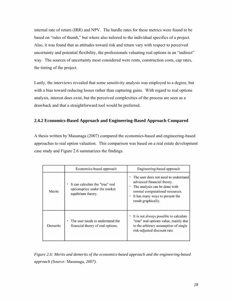
A thesis written by Masunaga (2007) compared the economics-based and engineering-based
approaches to real option valuation. This comparison was based on a real estate development
case study and Figure 2.6 summarizes the findings.
Figure 2.6: Merits and demerits of the economics-based approach and the engineering-based
approach (Source: Masunaga, 2007).
29
These results reiterate the differences between the two methods and also highlight the
advantages of the engineering based approach with respect to professional practice, while
qualifying this notion based on a singular risk-adjusted discount rate. Masunaga also
concludes that the engineering-based approached could be used to present an investment
opportunity to certain audiences, but backed-up by the results of the economics-based
approach. This suggestion is derived from a discrepancy (8%) in the calculation of true land
value between the methods.
Additionally looking at both valuation approaches within their research Barman and Nash
(2007) concluded that a “hybrid model” incorporating aspects of the two techniques.
Specifically, the Samuelson-McKean hurdle value was implemented as a factor in the
flexibility decision criteria.
Although both conclusions recommend in some way that the engineering-based model be
augmented with the economics approach, these conclusion may begin to detract from the
straightforward nature of the spreadsheet analysis. Considering that the differences found
between the two approached can be considered small, the engineering-based approach
produces fairly accurate results when compared to rigorous economic theory. Also, when
compared to a valuation method which might ignore flexibility all together, the strength
of the model as a tool for practitioners grows significantly. Given these considerations
and the real world applicability of analyzing the HCSC headquarters as a case study, the
engineering-based approach was implemented in valuing the flexibility associated with
vertical expansion.
30
Chapter 3: HCSC Headquarters
To investigate the potential of flexibility in real estate and the real options engineering-based
approach to valuation, the Health Care Service Corporation tower in Chicago, IL will be
analyzed as an examination of how these concepts can be applied to a conceived and
executed development project.
The information presented in this chapter was gathering from interviews with Jim D'Amico,
Joseph Dolinar, David Eckmann, Andrew Pini, Lou Rossetti, and Bud Spiewak; on-site
observations by the author; and materials provided by the architect.
3.1 Project Description
The HCSC project and the ultimate decision to construct a tower with an embedded option to
expand evolved out of the interactions of many contributing factors. These include the
corporate goals of the HCSC, the space market of Chicago in general, and availability and
characteristics of developable land in downtown Chicago.
3.1.1 History
In 1992, HCSC began to consider a plan for the future growth of the company and
anticipated its associated space needs. At that time, the company was leasing approximately
500,000 square feet of office space in downtown Chicago to accommodate 3000 employees.
The company projected their growth to reach 7200 employees over the following twenty-two
years, and the appropriate means of expanding their facilities was thought to be an important
factor to the successful future of their organization.
When beginning to assess the needs of the corporate growth and the potential options to
satisfy them, the following three major options were formulated: (1) attempt to lease
additional space in a building adjacent to the current facility, (2) lease (as a primary tenant)
space in a speculative office development, and (3) build and inhabit an new building
constructed to suit their specific needs.
31
Concurrently, the strategic motivations of the organization’s growth were such that a long
term consolidated central headquarters in downtown Chicago was considered to be a strong
asset for the future culture and identity of the corporation. Additionally, the commuting
patterns of a majority of their employees are centered on the current downtown location.
This fact contributed to an early decision to not consider a suburban location seriously.
When comparing the options available for expansion to the motivating factors of the
organization, the ultimate decision was distilled in the process. Leasing additional space in a
neighboring building would not achieve their goals for a synergetic consolidation of business
groups. Also, the availability of downtown Chicago office space of the scale required by
HCSC at the time would have made assembling leasable space in an efficient manner
challenging.
Acknowledging themselves as a singular large tenant, it was thought that adopting a
speculative office development would not accommodate the specific and well established
organizational structures of the company, and lead to potential inefficiencies (Figure 3.1).
With these two conclusions and a concurrent investigation of potentially available and
appropriate land underway, the decision to build for themselves was eventually reached.
32
Figure 3.1: Comparison of the typical speculative office building characteristics with the
requirements of HCSC (BCBS) (Source: Goettsch Partners, 2008).
3.1.2 Site Characteristics
The site selected was a 100,000 square foot (SF) piece of land at 300 East Randolph Street,
within a few blocks of the existing space leased by HCSC (Figure 3.3). Located at prominent
destination in downtown Chicago, the site is across from Grant Park (and at the time the
future Millennium Park), next to the Aon Center (formerly the Standard Oil Building), and
close to several other large buildings and headquarters. Also, the site’s proximate location to
the existing facility allowed for a minimum impact with respect to the employees. The site, a
portion of a much larger area of land, is located on a former rail yard (Figure 3.4) and
designated as a planned unit development (PUD) by the zoning authorities of Chicago. A
PUD is typically a single area designated for the development of a variety of complementary
land uses which are often different from previous zoning decisions. Additionally, the
development of a PUD allows for a modified negotiating process between developers and the
municipality with efforts to benefit the goals of both parties. The developer can benefit from
allowance of higher densities and synergetic relationships between uses which adds value to
all of the smaller sites contained within. The benefit to the municipality is in achieving a
specific economic and/or urban planning goal for a particular area of a city.

33
Figure 3.3: Project location plan, structure circled (Source: Goettsch Partners, 2008).
In the case of the PUD containing the HCSC site, the regulations allowed for a transfer of
density, floor area ratio (FAR), between the individual parcels within the larger area. FAR is
the ratio of the total floor area of a building(s), to the total area of the parcel of land it
occupies. This is facilitated by purchasing the additional density from other parcels and
adding it to a specific one. The 100,000 SF project site was originally zoned for density of
10 FAR. With the goal of building more area on the same size site, density was purchased to
allow for building to an FAR of 18. Increased density on and urban site, like in Chicago, is
typically considered more valuable intrinsically. With regard to HCSC, the increasing the
density to 18 FAR was related to two particular factors. The first factor was their demand for
enough density to satisfy the space requirements of the organization. The second factor was
that the terms of the parcel within the PUD dictated that building at a density greater than 18
FAR would require the developer to also provide a park on the site at a significant cost. The
land and additional density was purchased in 1994.
34
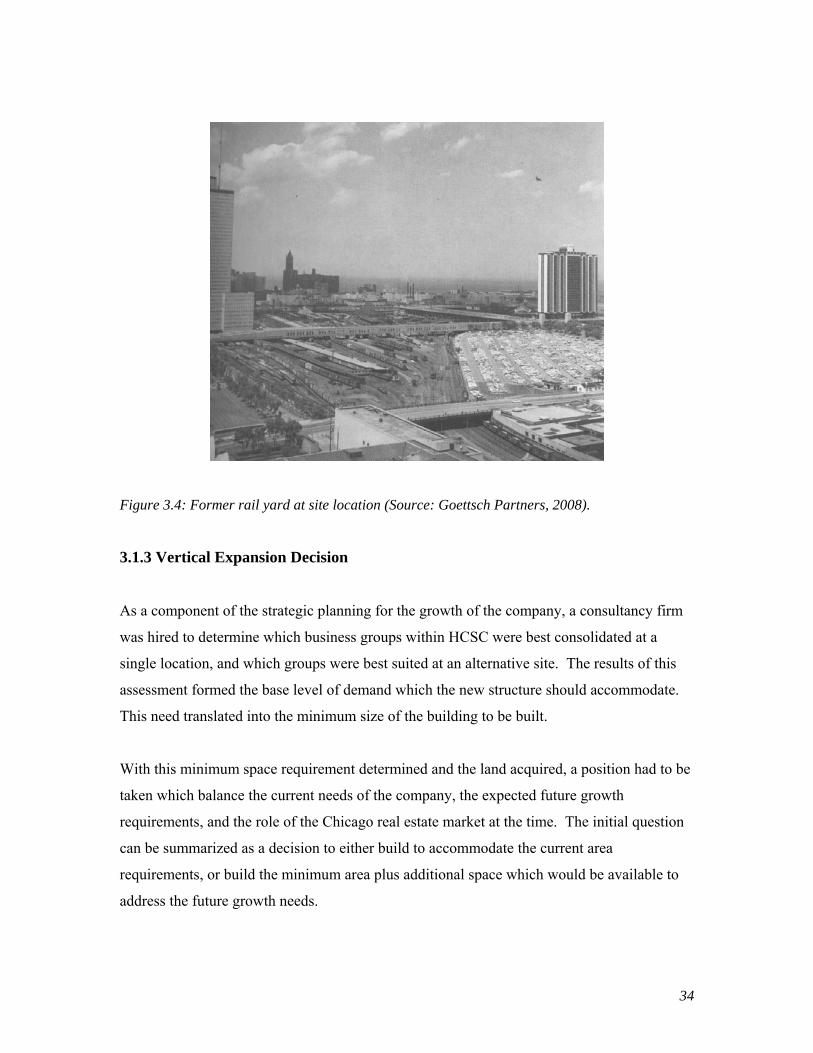
Figure 3.4: Former rail yard at site location (Source: Goettsch Partners, 2008).
3.1.3 Vertical Expansion Decision
As a component of the strategic planning for the growth of the company, a consultancy firm
was hired to determine which business groups within HCSC were best consolidated at a
single location, and which groups were best suited at an alternative site. The results of this
assessment formed the base level of demand which the new structure should accommodate.
This need translated into the minimum size of the building to be built.
With this minimum space requirement determined and the land acquired, a position had to be
taken which balance the current needs of the company, the expected future growth
requirements, and the role of the Chicago real estate market at the time. The initial question
can be summarized as a decision to either build to accommodate the current area
requirements, or build the minimum area plus additional space which would be available to
address the future growth needs.
35
Any additional space beyond the amount taken by HSCS would be expected to lease in the
market at rents which are high enough to justify the additional expense of constructing it. In
1995 when these decisions were being weighed, the office market in Chicago had been
declining and it was thought that the possibility of leasing the extra office space at the
required rents would be challenging. Recent history at the time would have encouraged a
pessimistic view of the near future market conditions.
At the same time, HCSC anticipated growth internally and desired to keep their headquarters
consolidated at the newly designated downtown site. The disconnect between planning for
future growth at one location and lacking the ability to temporarily fill the additional space
led to the idea of providing the potential to expand the project vertically at a point in the
future.
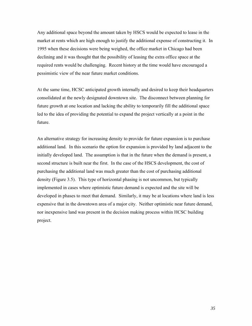
An alternative strategy for increasing density to provide for future expansion is to purchase
additional land. In this scenario the option for expansion is provided by land adjacent to the
initially developed land. The assumption is that in the future when the demand is present, a
second structure is built near the first. In the case of the HSCS development, the cost of
purchasing the additional land was much greater than the cost of purchasing additional
density (Figure 3.5). This type of horizontal phasing is not uncommon, but typically
implemented in cases where optimistic future demand is expected and the site will be
developed in phases to meet that demand. Similarly, it may be at locations where land is less
expensive that in the downtown area of a major city. Neither optimistic near future demand,
nor inexpensive land was present in the decision making process within HCSC building
project.
36
Figure 3.5: Land cost with respect to vertical or horizontal expansion options. Note: Actual
dollar amounts were redacted (Source: Adopted from Goettsch Partners, 2008).
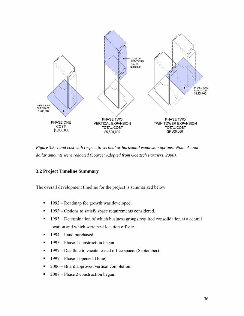
3.2 Project Timeline Summary
The overall development timeline for the project is summarized below:
1992 – Roadmap for growth was developed.
1993 – Options to satisfy space requirements considered.
1993 – Determination of which business groups required consolidation at a central
location and which were best location off site.
1994 – Land purchased.
1995 – Phase 1 construction began.
1997 – Deadline to vacate leased office space. (September)
1997 – Phase 1 opened. (June)
2006 – Board approved vertical completion.
2007 – Phase 2 construction began.

37
3.3 Building Specifications
Following the decision to develop a vertically expandable structure, the overall building
(Phase 1 and Phase 2 combined) was designed to maximize the allowable FAR assembled for
the site. The scale of the first phase was based on accommodating the present HCSC needs,
and the second phase was to occupy the remainder. The building occupies the corner of E.
Randolph and N. Columbus (Figure 3.6) with a direct link to underground parking below
Grant Park and easy walking access to mass transit nodes. With adjacencies to the park and
the overall plan of the PUD, and situated in an intermediate position between shore of Lake
Michigan and the heart of downtown Chicago; the building offers spectacular views in all
directions.
Figure 3.6: Site Plan (Source: Goettsch Partners, 2008)
The characteristics of the different phases are summarized in the following table (Table 3.1):
Gross Area Gross Area FAR Rentable Square FeetLevels
(Above Grade)
Phase 1 1,430,718 1,343,677 1,047,822 29
Phase 2 883,453 798,526 704,717 25
Total 2,314,171 2,142,203 1,752,539 54 Table 3.1: Building space characteristics (Source: Goettsch Partners, 2008).

38
The building is a steel frame structure with lateral bracing provided by concrete shear walls
for Phase 1 (levels one through twenty-nine), and cross bracing for Phase 2 (levels thirty
through fifty-four). The exterior of the structure is clad in glass and natural stone. The
aesthetic considerations of both phases were carefully articulated to achieve a very consistent
visual appearance in the event that the expansion option was exercised (Figure 3.7).
Figure 3.7: Architect’s renderings of Phase 1 and Phase 2 (Source: Goettsch Partners, 2008).
3.4 Real Options “in” Projects
To provide the option for future vertical expansion or completion, the first phase of the
project must be engineered and constructed to accommodate the expansion. An architectural
design executed in the manner presents an example of a real option “in” a project, and in
contrast to real options “on” projects (Wang and de Neufville, 2005). Wang and de Neufville
discuss the differences between these two types of option, and the primary points are
summarized in Figure 3.8.
39
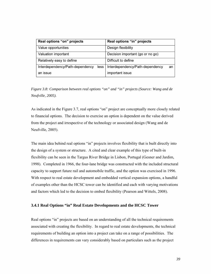
Figure 3.8: Comparison between real options “on” and “in” projects (Source: Wang and de
Neufville, 2005).
As indicated in the Figure 3.7, real options “on” project are conceptually more closely related
to financial options. The decision to exercise an option is dependent on the value derived
from the project and irrespective of the technology or associated design (Wang and de
Neufville, 2005).
The main idea behind real options “in” projects involves flexibility that is built directly into
the design of a system or structure. A cited and clear example of this type of built-in
flexibility can be seen in the Targus River Bridge in Lisbon, Portugal (Gesner and Jardim,
1998). Completed in 1966, the four-lane bridge was constructed with the included structural
capacity to support future rail and automobile traffic, and the option was exercised in 1996.
With respect to real estate development and embedded vertical expansion options, a handful
of examples other than the HCSC tower can be identified and each with varying motivations
and factors which led to the decision to embed flexibility (Pearson and Wittels, 2008).
3.4.1 Real Options “in” Real Estate Developments and the HCSC Tower
Real options “in” projects are based on an understanding of all the technical requirements
associated with creating the flexibility. In regard to real estate developments, the technical
requirements of building an option into a project can take on a range of possibilities. The
differences in requirements can vary considerably based on particulars such as the project

40
type (residents, office, industrial, etc.), the scale of the project, site characteristics, regulatory
/ entitlement processes, building codes, and any of the other forces that contribute to shaping
a property development.
In order to build the flexibility to expand from twenty-nine to fifty-four levels, the HSCS
headquarters had its own set of particular characteristics which had to be considered in the
design. Some of the particulars are inherent in the vertical nature of the building and others
related to the specific needs of the owner and the City of Chicago building code. Being a tall
and complex structure, the technical considerations enabling flexibility in the HCSC tower
range from large provisions in the overall structural design, to a plethora of smaller items
such as a modified width dimension along egress routes with in anticipation of an updated
life safety code. To describe them all would be lengthy and somewhat redundant. To gain a
perspective on additional provisions built into the first phase of the project, specific aspects
of the following four major building systems will be discussed: the structural design, the
mechanical design (HVAC, plumbing, electrical), vertical circulation (elevators and stairs),
and the exterior cladding.
Probably the first system to come to mind when imagining the concept of adding an
additional twenty-four stories to an existing building is overall structure. In the HSCS tower
at the most fundament level, the vertical structural members (columns) of the building had to
be oversized to accommodate the additional gravity loads of the extension. Also, the
building’s foundations had to be sized for the additional load. The foundations of the
structure are bell caissons at a depth of ninety feet, and incidentally the largest ones available
at the time. In addition to providing adequate structural capacity in the first phase to
accommodate the extension, the means to fasten the future columns to the exist one ones was
essential. To allow for this future connection, the tops of the columns were extended through
the slab and membrane of the first phase roof and waterproofed around (Figure 3.9).
41
Figure 3.9: Top of Phase 1 column extended through the roof slab and waterproofed to facilitate
a connection for the Phase 2 expansion (Source: Goettsch Partners, 2008).
This detail allowed the new structure to be welded to the existing (Figure 3.10), and in a way
which minimally impacts the existing roof which is beneficial given that construction of the
expansion was always intended to occur over a fully occupied building.

42
Figure 3.10: Welded connection of the new and existing structure at the Phase 1 roof level
(Source: Author).
In addition to the enhanced structure and foundations, the mechanical systems of the building
required oversized provisions to accommodate the additional loaded in the future. Some of
these provisions included space for extra sleeves in risers for future electrical cabling, larger
pipes, and a fire sprinkler pumping strategy to accommodate the additional future spaces.
The vertical circulation system presented an interesting challenge for designers since the
number of elevators would need to increase from sixteen to thirty-two. Planning for such an
addition requires providing the necessary amount of physical space and in a way such that the
logic of the circulation through the building remains practical and efficient. To accomplish
this goal, the building was designed with a large full height atrium on the north side of the
structure, flanked by the Phase 1 elevators. This arrangement allows for the future elevators
to be installed in a portion of the atrium space while also leaving portion of space remaining
for daylight to continue migrating through the core (Figures 3.11 and 3.12). Lastly, from an
exterior aesthetic point of view, the materials of the cladding system were strategically

43
designed. The stone selected for the façade was from a quarry with a seemingly sufficient
supply to satisfy the demands of the future addition.
Figure 3.11: Typical floor place with Phase 1 and Phase 2 elevator arrangement indicated
(Source: Goettsch Partners, 2008).

44
Figure 3.12: Phase 1 atrium and Phase 2 elevators under construction in provided space
(Source: Goettsch Partners, 2008).
The technical enhancements to the first phase of the project were the result a strong forward
thinking approach to the design, creative architectural and engineering solutions, and an
overall commitment to the success of the potential future expansion. While this additional
work was required to build-in the flexibility and did incur the cost of providing the option,
the overall physical contribution to the project does not fall too far outside of typical design
and construction for a structure of this type.
45
Chapter 4: Real Options Analysis of the HCSC Headquarters
This chapter describes the real options analysis based on the characteristics of the built-in
option to vertically expand the HCSC tower. To reiterate, the “engineering-based” approach
was selected as the valuation methodology based on the following points which link the real
options analysis to traditional real estate finance:
o The implicit common language the two methods of valuation.
o The use of Excel® and standard spreadsheet modeling as a commonly understood
tool.
o The transparency and similarity of the inputs.
o The intuitively understandable nature of the output metrics and clarity of the visual
results.
4.1 Methodology
The main structure of the methodology is formed by the following steps:
1) Define the assumptions for the overall model.
2) Define the uncertain variables, and the decision making structure for the flexible case.
3) Valuation of the three different scenarios;
a. Phase 1 (twenty-nine levels) only.
b. Phase 1 and Phase 2 (fifty-four levels) as one complete structure.
c. Valuation of a flexible design which incorporates the option to expand the
structure vertically (from twenty-nine to fifty-four levels) under specified
conditions.
4) Interpretation of the results using value at risk or gain (VARG) curves.
The three valuations will be simultaneously compared to determine the potential value that
flexibility brings (or perhaps not bring) to the project. Expected net present values (ENPV)
are simulated for each of these scenarios under the same conditions of uncertainty.

46
4.2 Assumptions
To provide the requisite inputs to the real options model, certain assumptions based on
market conditions are made. Also, simplifications to the overall building design are
incorporated to allow for a slightly more straightforward approach to the modeling. These
simplifications to the structure involve assuming that the rentable areas of both phases of the
project are the same (Table 4.1), or in other words, each phase comprises 50% of the entire
potential structure.
Gross Area Rentable Square Feet
Phase 1 1,520,000 1,000,000
Phase 2 1,250,000 1,000,000
Total 2,770,000 2,000,000
Table 4.1: Simplified building program for analytical purposes.
The gross area is based on the relative proportions of rentable to gross areas as in the actual
HCSC structure. The greater gross area of the first phase is based on the below grade spaces
dedicated to the service needs of the building. The gross areas are used in the calculation of
the total costs, and the rentable areas are the basis for revenue calculation.
Additional assumptions used in the analysis are the following:
o The analysis is from an ex-post perspective beginning in 1997, the completion date of
Phase 1.
o Initial rents are $24 per square foot (based on historical data for 1997 Class A office
rent in downtown Chicago).
o The risk free interest rate (rƒ) is 4.85% (calculated from the 1997 average ten year
U.S. Treasury rate, 6.35%, minus 150 basis points).
o The risk premium for stabilized Class A office space is 3.50%.
o The project discount rate is 8.35% (calculated as r = rƒ - + RP).
o Development cost growth is 1.50%.

47
o Operating expenses are $7.50 per square foot.
o Cap rates are 7.50% (based on 2007 average for downtown Chicago office
properties).
o Development costs are $140 per square foot for Phase 1 and $124 for Phase 2. The
additional cost per square foot to develop Phase 1 accounts for the cost of the land.
o Phase 2 construction time is 2 years.
4.3 Uncertain Variables and Decision Rules
To consider the uncertain nature of the future and its potential implications on the value of a
real estate development, the model must incorporate measures indicative of possible future
scenarios. To incorporate relevant uncertain variables into the analysis, factors were chosen
to represent the varying nature of (1) future cash flows and (2) demand for office space. To
represent these two variables, uncertainty in the projected future achieved rents (cash flow)
and the future lease-up rates of the building (office space demand) are considered.
4.3.1 Projected Rent
To incorporate the uncertainty in potential future rent growth, the initial rent for Chicago in
1997 of $24 per square foot was subjected to a series of volatilities to simulate a wide range
of potential future rent patterns. This base rent was expected to grow at 1% per year. This
1% growth rate is based on the fact that during the 1978-2004 period, the average annual
growth of net operating income for institutional and commercial properties held in the
NCREIF database was approximately 2% less than average annual inflation (Geltner et al,
2007). With inflation assumed to be 3% for the purposes of this analysis, 3% - 2% = 1%.
After this determination of a base rent and expected growth, volatilities were applied to
provide a range of possible uncertainty for which the flexible case can react. The steps used
in this model are the following:

48
1) The Expected Rent was calculated by growing the base rent at 1% (Eg) per year with
a standard deviation of .35% (SDg) to determine a Realized Rent.
Expected Rent = Rent(T-1) (1 + Eg)
SGg Realized = (rand() + rand() - 1) (2) (SDg)
Realized Rent = Rent(T-1) (1 + Eg + Sg Realized)
2) To determine a Trend Rent, a volatility which accumulates over time of 4% (σ) was
applied to each year.
σ(T) = (rand() + rand() -1 ) (2) (σ)
Trend Rent = Rent(T-1) (1 + Eg + SDg + σ(T))
3) To introduce potential volatility at each individual period noise of 8% was applied to
each year to arrive at the Achieved Rent.
noise(T) = (rand() + rand() - 1) (2) (noise)
Achieved Rent = Trend Rent(T) (1 + noise(T))
For this analysis, the initial base rent of $24 per square foot was the approximate rate for
downtown Chicago office buildings in 1997 and the expected growth rate was assumed to be
1%. The remainder of the variables which provide uncertainty and variability were selected
to (1) provide a rich representation of potential future rent growth scenarios, (2) describe a
methodology, and (3) demonstrate the value of flexibility with respect to uncertain
conditions. Alternatively, the variables could be determined through a rigorous analysis of
the historic rents for a given market.
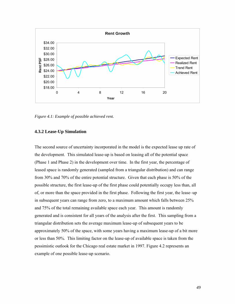
49
Rent Growth
$18.00$20.00$22.00$24.00$26.00$28.00$30.00$32.00$34.00
0 4 8 12 16 20Year
Ren
t PSF
Expected RentRealized RentTrend RentAchieved Rent
Figure 4.1: Example of possible achieved rent.
4.3.2 Lease-Up Simulation
The second source of uncertainty incorporated in the model is the expected lease up rate of
the development. This simulated lease-up is based on leasing all of the potential space
(Phase 1 and Phase 2) in the development over time. In the first year, the percentage of
leased space is randomly generated (sampled from a triangular distribution) and can range
from 30% and 70% of the entire potential structure. Given that each phase is 50% of the
possible structure, the first lease-up of the first phase could potentially occupy less than, all
of, or more than the space provided in the first phase. Following the first year, the lease–up
in subsequent years can range from zero, to a maximum amount which falls between 25%
and 75% of the total remaining available space each year. This amount is randomly
generated and is consistent for all years of the analysis after the first. This sampling from a
triangular distribution sets the average maximum lease-up of subsequent years to be
approximately 50% of the space, with some years having a maximum lease-up of a bit more
or less than 50%. This limiting factor on the lease-up of available space is taken from the
pessimistic outlook for the Chicago real estate market in 1997. Figure 4.2 represents an
example of one possible lease-up scenario.
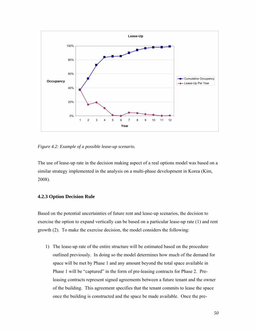
50
Figure 4.2: Example of a possible lease-up scenario.
The use of lease-up rate in the decision making aspect of a real options model was based on a
similar strategy implemented in the analysis on a multi-phase development in Korea (Kim,
2008).
4.2.3 Option Decision Rule
Based on the potential uncertainties of future rent and lease-up scenarios, the decision to
exercise the option to expand vertically can be based on a particular lease-up rate (1) and rent
growth (2). To make the exercise decision, the model considers the following:
1) The lease-up rate of the entire structure will be estimated based on the procedure
outlined previously. In doing so the model determines how much of the demand for
space will be met by Phase 1 and any amount beyond the total space available in
Phase 1 will be “captured” in the form of pre-leasing contracts for Phase 2. Pre-
leasing contracts represent signed agreements between a future tenant and the owner
of the building. This agreement specifies that the tenant commits to lease the space
once the building is constructed and the space be made available. Once the pre-
Lease-Up
0%
20%
40%
60%
80%
100%
1 2 3 4 5 6 7 8 9 10 11 12
Year
Occupancy Cumulative OccupancyLease-Up Per Year

51
leasing contracts amount to a designated percentage of the total space provided by
Phase 2, the criterion to exercise the option is met. In other words, if each contract is
placed in a folder after being signed, once the folder is thick enough; Phase 2 of the
structure will be built. This process is diagramed in Figure 4.3. Although applying
the concept of pre-leasing contracts in this manner may appear to be an abstraction
from reality, the argument could be made that such leasing characteristics would be
indicative of a strong office rental market in which the space might be leased even if
such contracts are broken. Also, the amount of pre-leasing contracts deemed to be
acceptable is somewhat subjective and based on the individual preferences of the
developer.
2) The compound annual growth rate of the rent is calculated each year and compared to
a specified hurdle. The hurdle should be determined by an assumed acceptable rent
growth by which a developer would feel comfortable to use as basis for future rent.
The first year in which both of these two criteria are met will trigger the exercise of the
option.
Figure 4.3: Decision rule diagram (Illustration by Author).

52
A numerical example of the simulated data that makes up the criteria for the decision to exercise
the expansion option is represented in Figures 4.4 (A) and (B) below. Figure 4.4 (A) is the lease-
up pattern of the entire structure which will determine the expansion decision. The graph in
Figure 4.4 (B) represents the associated lease up pattern as it relates to the total structure, Phase 1,
and the pre-leasing contracts for Phase 2.

53
(A) Lease-up rate.
1 2 3 4 5 6 7 8 9 10
0%
10%
20%
30%
40%
50%
60%
70%
80%
90%
100%
% o
f Tot
al D
evel
opm
ent
Year
Total Development Lease-Up
Remainder of Total to be Leased
% of Total as P2 Pre-LeasingContracts% of Total From P1
(B) Cumulative total lease-up and lease-up per phase.
Figure 4.4: Example of a possible lease-up scenario.
Lease-Up
0%
40%
80%
100%
1 2 3 4 5 6 7 8 9 10
Year
Occupancy Cumulative Occupancy
Lease-Up Per Year
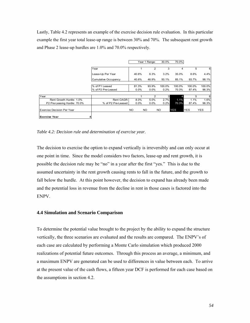
54
Lastly, Table 4.2 represents an example of the exercise decision rule evaluation. In this particular
example the first year total lease-up range is between 30% and 70%. The subsequent rent growth
and Phase 2 lease-up hurdles are 1.0% and 70.0% respectively.
Year 1 Range: 30.0% 70.0%
Year 1 2 3 4 5 6
Lease-Up Per Year 40.6% 6.3% 3.2% 35.0% 8.6% 4.4%
Cumulative Occupancy 40.6% 46.9% 50.1% 85.1% 93.7% 98.1%
% of P1 Leased 81.3% 93.9% 100.0% 100.0% 100.0% 100.0%% of P2 Pre-Leased 0.0% 0.0% 0.2% 70.3% 87.4% 96.3%
Year 1 2 3 4 5 6Rent Growth Hurdle: 1.0% Rent CAGR: 8.0% 5.0% 2.7% 1.1% 1.1% 1.6%
P2 Pre-Leasing Hurdle: 70.0% % of P2 Pre-Leased: 0.0% 0.0% 0.2% 70.3% 87.4% 96.3%
Exercise Decision Per Year NO NO NO YES YES YES
Exercise Year 4
Table 4.2: Decision rule and determination of exercise year.
The decision to exercise the option to expand vertically is irreversibly and can only occur at
one point in time. Since the model considers two factors, lease-up and rent growth, it is
possible the decision rule may be “no” in a year after the first “yes.” This is due to the
assumed uncertainty in the rent growth causing rents to fall in the future, and the growth to
fall below the hurdle. At this point however, the decision to expand has already been made
and the potential loss in revenue from the decline in rent in those cases is factored into the
ENPV.
4.4 Simulation and Scenario Comparison
To determine the potential value brought to the project by the ability to expand the structure
vertically, the three scenarios are evaluated and the results are compared. The ENPV’s of
each case are calculated by performing a Monte Carlo simulation which produced 2000
realizations of potential future outcomes. Through this process an average, a minimum, and
a maximum ENPV are generated can be used to differences in value between each. To arrive
at the present value of the cash flows, a fifteen year DCF is performed for each case based on
the assumptions in section 4.2.
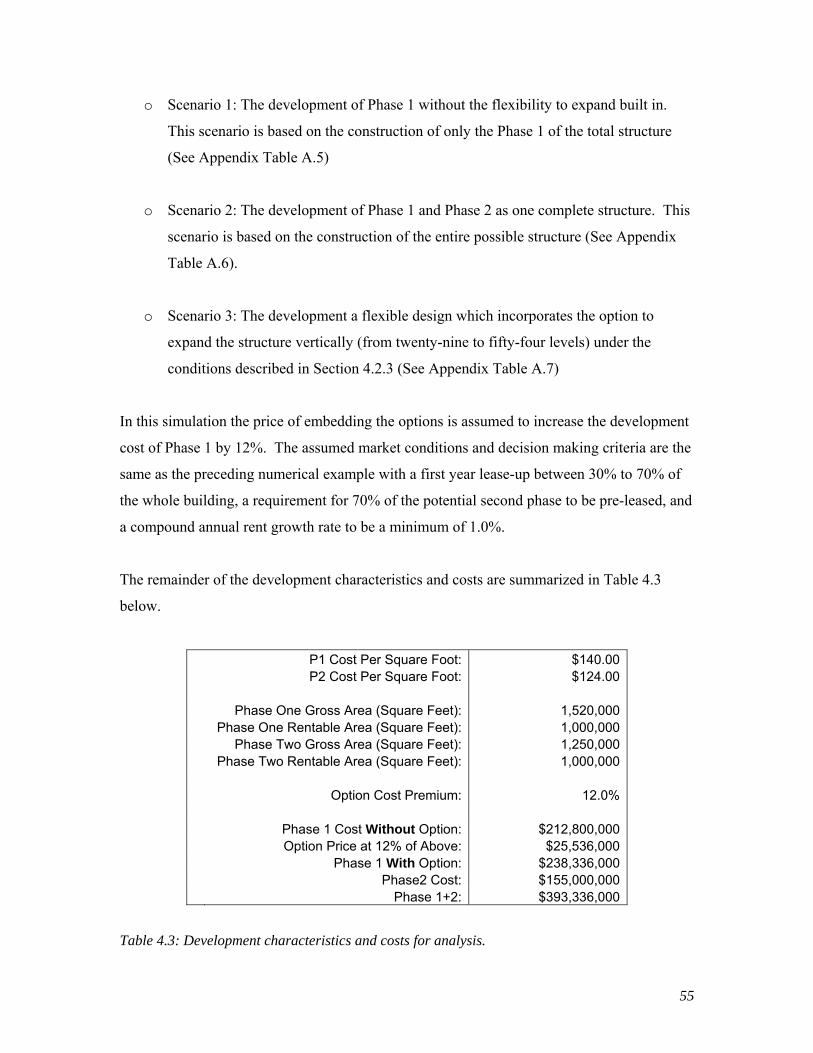
55
o Scenario 1: The development of Phase 1 without the flexibility to expand built in.
This scenario is based on the construction of only the Phase 1 of the total structure
(See Appendix Table A.5)
o Scenario 2: The development of Phase 1 and Phase 2 as one complete structure. This
scenario is based on the construction of the entire possible structure (See Appendix
Table A.6).
o Scenario 3: The development a flexible design which incorporates the option to
expand the structure vertically (from twenty-nine to fifty-four levels) under the
conditions described in Section 4.2.3 (See Appendix Table A.7)
In this simulation the price of embedding the options is assumed to increase the development
cost of Phase 1 by 12%. The assumed market conditions and decision making criteria are the
same as the preceding numerical example with a first year lease-up between 30% to 70% of
the whole building, a requirement for 70% of the potential second phase to be pre-leased, and
a compound annual rent growth rate to be a minimum of 1.0%.
The remainder of the development characteristics and costs are summarized in Table 4.3
below.
P1 Cost Per Square Foot: $140.00 P2 Cost Per Square Foot: $124.00 Phase One Gross Area (Square Feet): 1,520,000 Phase One Rentable Area (Square Feet): 1,000,000 Phase Two Gross Area (Square Feet): 1,250,000 Phase Two Rentable Area (Square Feet): 1,000,000 Option Cost Premium: 12.0% Phase 1 Cost Without Option: $212,800,000 Option Price at 12% of Above: $25,536,000 Phase 1 With Option: $238,336,000 Phase2 Cost: $155,000,000 Phase 1+2: $393,336,000
Table 4.3: Development characteristics and costs for analysis.

56
The main intent of this analysis is to investigate the value that flexibility brings to project
designed for vertical expansion. In this example the options was exercised in Year 4 of the
analysis when Phase 2 of the development was 84.4% pre-leased and the compound annual
rent growth was 1.9% (Table 4.4).
Year 1 Range: 30.0% 70.0%
Year 1 2 3 4 5 6
Lease-Up Per Year 44.6% 27.5% 12.5% 3.1% 4.4% 5.4%
Cumulative Occupancy 44.6% 72.1% 84.7% 87.8% 92.2% 97.6%
% of P1 Leased 89.3% 100.0% 100.0% 100.0% 100.0% 100.0%% of P2 Pre-Leased 0.0% 44.2% 69.3% 75.5% 84.4% 95.2%
Year 1 2 3 4 5 6Rent Growth Hurdle: 1.0% Rent CAGR: -10.4% -2.7% -1.4% 0.4% 1.9% -1.7%
P2 Pre-Leasing Hurdle: 70.0% % of P2 Pre-Leased: 0.0% 44.2% 69.3% 75.5% 84.4% 95.2%
Exercise Decision Per Year NO NO NO NO YES NO
Exercise Year 5
Table 4.4: Simulation decision.
The results of this simulation are described in Table 4.4. It numerically displays how
flexibility can affect the valuation of a development. In this example the flexible condition
increased the ENPV by approximately $10 million (from 22,025 to 31,761 million) over
simply building the first phase. This gain represents the exercising of the option at the
appropriate time. Concurrently, the flexible design limits the potential downside loss
associated with building the entirety of Phase 1 and Phase 2 initially by approximately $12
million in the worse case scenario (from -64,367 to -52,294 million).
(x 1000) Phase 1 Phase 1+2 Flexible
Initial Investment $212,800 $393,336 $238,336Expected NPV $22,025 $40,011 $31,761Maximum NPV $78,379 $152,014 $119,019Minimum NPV -$37,222 -$64,367 -$52,294
Return on Investmen 10.4% 10.2% 13.3%
Scenario
Table 4.5: Analysis results.

57
The return on investment is based (ROI) on the initial investment and the expected NPV
(Initial Investment / Expected NPV). The initial investment for the flexible case is slightly
larger that Phase 1, as the cost to purchase the option represents the increase. While
calculating the ROI in this way is a bit simplistic, it underscores the value created by
incorporating flexibility in a development project. In this example, the return on the initial
investment increases from 10.4% to 13.3% with the option to expand the structure vertically.
These same results are represented graphically by the VARG curves in Figure 4.5. In this
graphic, the curve representing the flexible case is shifted to the right with respect to both the
Phase 1 only and the Phase 1 + 2 scenarios. This relationship tells the same story as depicted
numerically in Table 4.4 above.
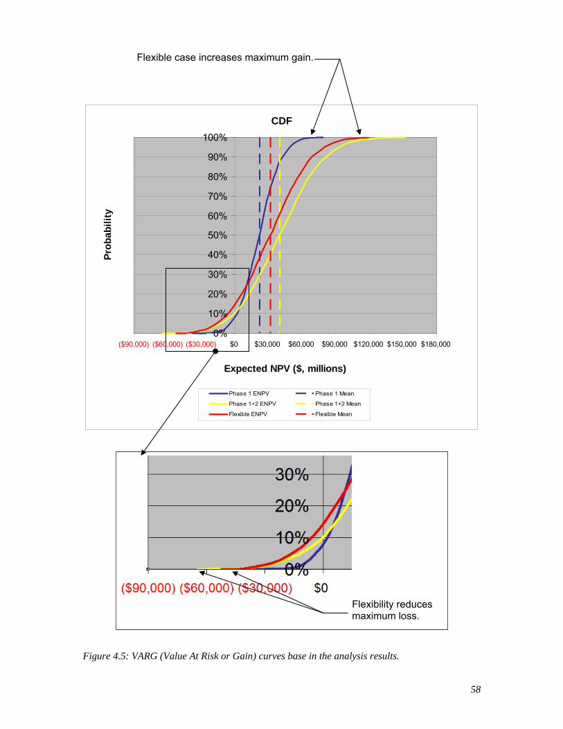
58
CDF
0%
10%
20%
30%
40%
50%
60%
70%
80%
90%
100%
($90,000) ($60,000) ($30,000) $0 $30,000 $60,000 $90,000 $120,000 $150,000 $180,000
Expected NPV ($, millions)
Prob
abili
ty
Phase 1 ENPV Phase 1 Mean
Phase 1+2 ENPV Phase 1+2 Mean
Flexible ENPV Flexible Mean
Figure 4.5: VARG (Value At Risk or Gain) curves base in the analysis results.
Flexible case increases maximum gain.
Flexibility reduces maximum loss.

59
While it is clear that building flexibility into a real estate development can have positive
implications on the overall value of the development, the outcome of the flexibility is
sensitive to many factors. These factors can be related to anything from the design or the
development costs, to the market and the preferences of the investor.
4.5 Analysis Observations
On the significant factors which could influence the value of the flexibility in a development
project is the cost of the option. In the preceding analysis, the premium paid for the option
increased the development cost by 12% and the resultant flexibility brought added value to
the project. Figure 4.6 represents a range of option premiums and the related effect on the
ENPV. The option premium is the additional cost of purchasing the option as a percentage
of the base total development cost. From the graph it can be see that at around 17%, the price
of the option prohibits the flexible case from adding value beyond that of the first phase. In
other words, the benefit of the flexibility may not be worth the cost of acquiring it. While
under the same conditions, the expected value of building the entire structure is still higher
than the smaller Phase 1, the downside exposure would be greater.
The option cost premium in this graphic represents the additional expense required to
construct Phase 2. For example, this expense includes the costs of providing greater capacity
structural, mechanical and vertical circulation systems. The costs associated with these
additional systems are required to provide the future option to expand vertically, but also are
necessary in the construction of Phase 1 + 2 together. Therefore, as the cost of providing the
option increases, the cost of building the Phase 1 + 2 scenario increases and the net present
values of both cases declines.
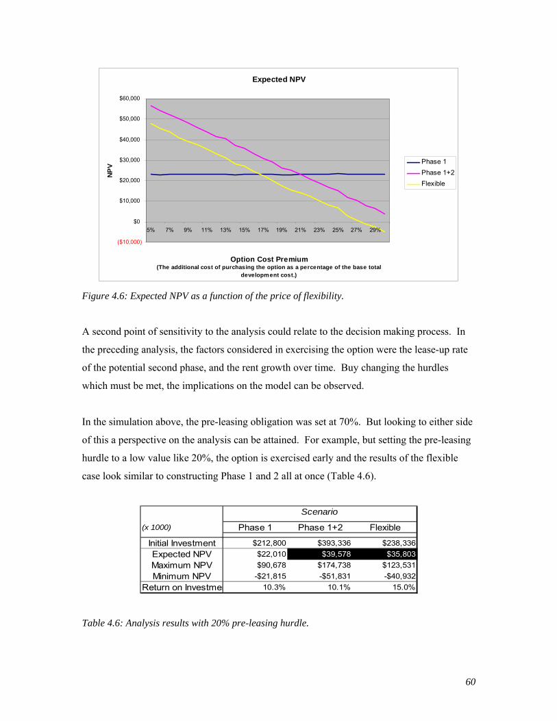
60
Expected NPV
($10,000)
$0
$10,000
$20,000
$30,000
$40,000
$50,000
$60,000
5% 7% 9% 11% 13% 15% 17% 19% 21% 23% 25% 27% 29%
Option Cost Premium(The additional cost of purchasing the option as a percentage of the base total
development cost.)
NPV Phase 1
Phase 1+2Flexible
Figure 4.6: Expected NPV as a function of the price of flexibility.
A second point of sensitivity to the analysis could relate to the decision making process. In
the preceding analysis, the factors considered in exercising the option were the lease-up rate
of the potential second phase, and the rent growth over time. Buy changing the hurdles
which must be met, the implications on the model can be observed.
In the simulation above, the pre-leasing obligation was set at 70%. But looking to either side
of this a perspective on the analysis can be attained. For example, but setting the pre-leasing
hurdle to a low value like 20%, the option is exercised early and the results of the flexible
case look similar to constructing Phase 1 and 2 all at once (Table 4.6).
(x 1000) Phase 1 Phase 1+2 Flexible
Initial Investment $212,800 $393,336 $238,336Expected NPV $22,010 $39,578 $35,803Maximum NPV $90,678 $174,738 $123,531Minimum NPV -$21,815 -$51,831 -$40,932
Return on Investmen 10.3% 10.1% 15.0%
Scenario
Table 4.6: Analysis results with 20% pre-leasing hurdle.
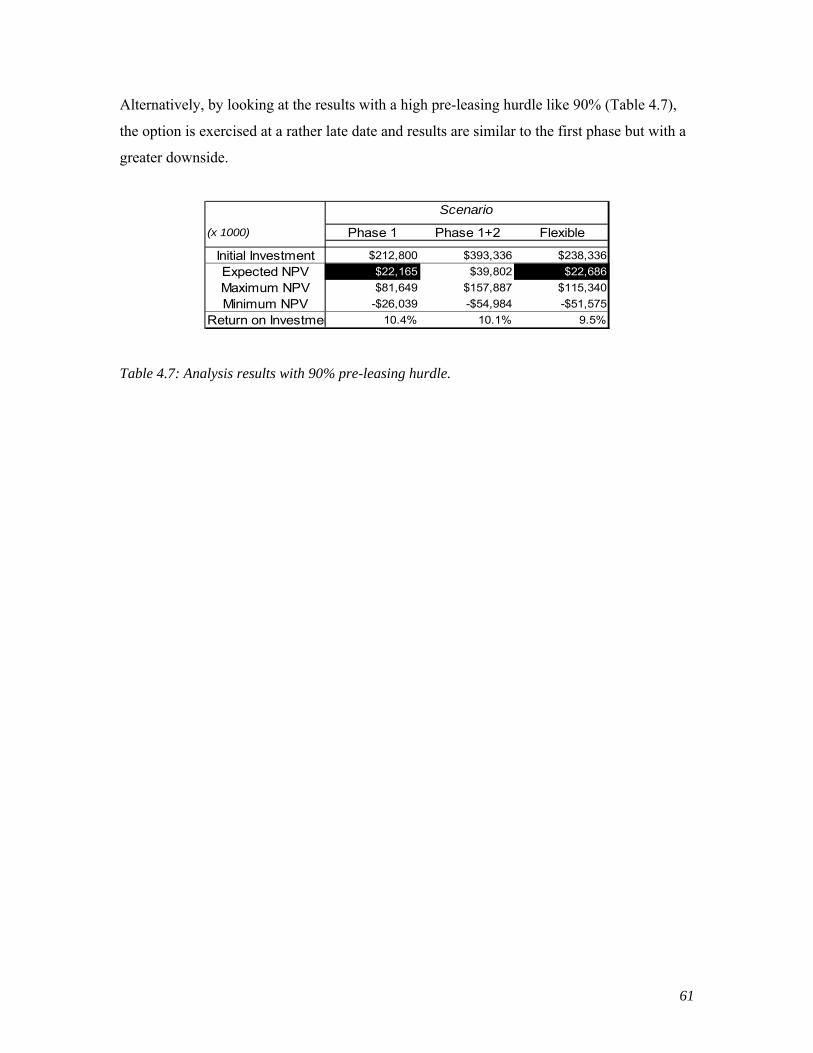
61
Alternatively, by looking at the results with a high pre-leasing hurdle like 90% (Table 4.7),
the option is exercised at a rather late date and results are similar to the first phase but with a
greater downside.
(x 1000) Phase 1 Phase 1+2 Flexible
Initial Investment $212,800 $393,336 $238,336Expected NPV $22,165 $39,802 $22,686Maximum NPV $81,649 $157,887 $115,340Minimum NPV -$26,039 -$54,984 -$51,575
Return on Investmen 10.4% 10.1% 9.5%
Scenario
Table 4.7: Analysis results with 90% pre-leasing hurdle.
62
Chapter 5: Conclusion
Although uncommon, vertically expandable structures are occasionally developed. While the
design, engineering, and construction process does present interesting and possibly unusual
challenges, most can typically be resolved through relatively convention means. Proper
planning and commitment to the ultimate long term goal of seeing the option realized is
essential to the overall success of the project.
All of these characteristics of vertical flexibility can easily be foreseen and the expectation of
a complex project would presumably be well anticipated. It is less clear however, what value
the flexibility will bring to a project and what type of financial analysis a developer might use
to quantify the potential value. The simple assumption is that efforts would be made to apply
tradition underwriting methods to the deal. That process along with the keen expertise of an
experienced developer might provide enough of feel for what the built-in flexibility is worth.
Concurrently, it is also easy to imagine that a seemingly more complex valuation
methodology such a real options analysis would not be considered in a typical real estate
practice. This may be true for a variety of reasons which range from a lack of understanding
to a perception complexity. While all of these points may be true, this thesis has
demonstrated that use of a real options analysis to value vertically expandable structures can
be performed with tools and metrics that are familiar to most all real estate professionals.
Additionally, applying these techniques to a vertically expandable structure can indeed
demonstrate that the flexibility can provide additional financial gain while limiting the
potential loss.
Flexibility in projects such as the HCSC headquarters does provide the ability to enhance the
maximum gain, limit the worst case loss, or improve the expected value. These facts
inherently point toward the idea that different types of investors have different preferences.
Some may be more interested in maximizing the potential upside of the development, and
others may be more interested in limiting downside losses. In the specific case of the HCSC
tower, the flexibility to expand also includes an intangible value associated with a singular
structure which can respond to the needs of a growing corporation.

63
Combining a tractable real option valuation methodology (spreadsheet analysis) with a
development strategy that includes the ability to exercise and a future option (e.g. vertical
expansion), the potential to match investor preferences to development projects becomes
enhanced. In applying the described methodology to a project which incorporates flexibility
the analytic expressions of interest to investors such as the value at risk, the expected and
maximum net present values, and the different returns based on the initial capital investments
are inherent products of the analysis. These metrics are valuable factors for developers
considering possible investments, and omitted from conventional NPV or DCF analyses.

64
Bibliography Worked Cited
Barman, B., Nash, K. E., (2007). A Streamlined Real Options Model for Real Estate Development. Unpublished Thesis S.M. in Real Estate Development --Massachusetts Institute of Technology Dept. of Urban Studies and Planning.
Borison, A. (2005). Real Options Analysis: Where Are the Emperor's Clothes? Journal of
Applied Corporate Finance, 17(2), 17-31. Brach, M. A. (2003). Real Options in Practice. Hoboken, N.J.: John Wiley & Sons. Brealey, R. A., Myers, S. C., & Allen, F. (2006). Principles of Corporate Finance (8th ed.).
New York, NY: McGraw-Hill/Irwin. Copeland, T., & Antikarov, V. (2001). Real Options: A Practitioner's Guide: New York:
Texere. de Neufville, R. (2002). Architecting/Designing Engineering Systems Using Real Options,
ESD-WP-2003-01.09. MIT Engineering Systems Symposium on the Intellectual Foundations of Engineering Systems. http://ardent.mit.edu/real_options/Real_opts_papers/ESD-WP-2003-01.09-ESD Internal Symposium.pdf
de Neufville, R., Scholtes, S., & Wang, T. (2006). Valuing Real Options by Spreadsheet:
Parking Garage Case Example. ASCE Journal of Infrastructure Systems, 12(2), 107-111.
Dixit, A. K., & Pindyck, R. S. (1994). Investment Under Uncertainty. Princeton, NJ:
Princeton University Press. Geltner, D., Miller, N., Clayton, J., & Eichholtz, P. (2007). Commercial Real Estate Analysis
& Investments (2nd ed.). Mason, OH: Thomson. Gesner, G., & Jardim, J. (1998). Bridge within a Bridge. Civil Engineering, 68(10), 44-47. Kim, K. (2008). Real Options: A Way to Deal with Market Uncertainty in Real Estate
Development Projects. Unpublished Thesis S.M. in Real Estate Development --Massachusetts Institute of Technology.
Leslie, K. J., & Michaels, M. P. (1997). The Real Power of Real Options. McKinsey
Quarterly (3), 4-22. Luehrman, T. A. (1998). Investment Opportunities as Real Options: Getting Started on the
Numbers. Harvard Business Review, 76(4), 51-67.

65
Masunaga, S., (2007). A Comparative Study of Real Options Valuation methods: Economics-Based Approach vs. Engineering-Based Approach. Unpublished Thesis S.M. in Real Estate Development --Massachusetts Institute of Technology Dept. of Urban Studies and Planning.
Pearson, J., & Wittels, K. (2008). Real Options in Action: Vertical Phasing in Commercial
Real Estate Development. Unpublished Thesis S.M. in Real Estate Development --Massachusetts Institute of Technology.
Sirmans, C. F. (1997). Research on Discounted Cash Flow Models. Real Estate Finance,
13(4), 93-95. Wang, T., & de Neufville, R. (2005). Real Options “in” Projects. 9th Real Options Annual
International Conference, Paris. http://ardent.mit.edu/real_options/Real_opts_papers/Real_Options_in_Projects-Tao-50217.pdf
Additional Reading Cardin, M.-A., (2007). Facing reality : design and management of flexible engineering
systems. Unpublished Thesis S.M. --Massachusetts Institute of Technology Engineering Systems Division Technology and Policy Program.
Childs, P. D., Riddiough, T. J., & Triantis, A. J. (1996). Mixed Uses and the Redevelopment
Option. Real Estate Economics, 24(3), 317-339. Cox, J. C., Ross, S. A., & Rubinstein, M. (1979). Option Pricing: A Simplified Approach.
Journal of Financial Economics, 7(3), 229-263. Coy, P. (1999). "Exploiting Uncertainty: The Real-Options Revolution in Decision Making “.
Business Week, 3632, 118–124. Ellingham, I., & Fawcett, W. (2006). New Generation Whole-Life Costing: Property and
Construction Decision-Making Under Uncertainty. London, UK: Taylor & Francis. Greden, L., (2005). Flexibility in Building Design: A Real Options Approach and Valuation
Methodology to Address Risk. Unpublished Thesis Ph. D. --Massachusetts Institute of Technology Dept. of Architecture.
Greden, L., & Glicksman, L. (2004). Options Valuation of Architectural Flexibility: A Case
Study of the Option to Convert to Office Space. Real Options 8th Annual International Conference, Montreal, Canada, 17–19. http://www.realoptions.org/papers2004/Greden_FlexibleDesign.pdf

66
Greden, L., & Glicksman, L. (2005). A Real Options Model for Valuing Flexible Space. Journal of Corporate Real Estate, 7(1), 34-48.
Hull, J. (2006). Options, Futures, and Other Derivatives (6th ed.). Upper Saddle River, N.J.:
Pearson/Prentice Hall. Myers, S. C. (1977). Determinants of Corporate Borrowing. Journal of Financial Economics,
5(2), 147-175. Oppenheimer, P. H. (2002). A Critique of Using Real Options Pricing Models in Valuing
Real Estate Projects and Contracts. Briefings in Real Estate Finance, 2(3), 221. Rocha, K., Salles, L., Garcia, F. A. A., Sardinha, J. A., & Teixeira, J. P. (2007). Real Estate
and Real Options -- A case study. Emerging Markets Review, 8(1), 67-79. Trigeorgis, L. (1993). Real Options and Interactions with Financial Flexibility. Financial
Management, 22(3), 202-224. Interviews Conducted D'Amico, Jim, The John Buck Company. In person interview. June 10-11, 2008. Interview
conducted by the author. Dolinar, Joseph, Goettsch Partners. In person interview. June 10-11, 2008. Interview
conducted by the author. Eckmann, David, Magnusson Klemencic. In person interview. June 11, 2008. Interview
conducted by the author. Pini, Andrew, Health Care Service Corporation. In person interview. June 12, 2008.
Interview conducted by the author.
Rossetti, Lou, Walsh Construction. In person interview. June 10, 2008. Interview conducted by the author. Spiewak, Bud, Cosentini Associates, Inc. In person interview. June 12, 2008. Interview
conducted by the author.
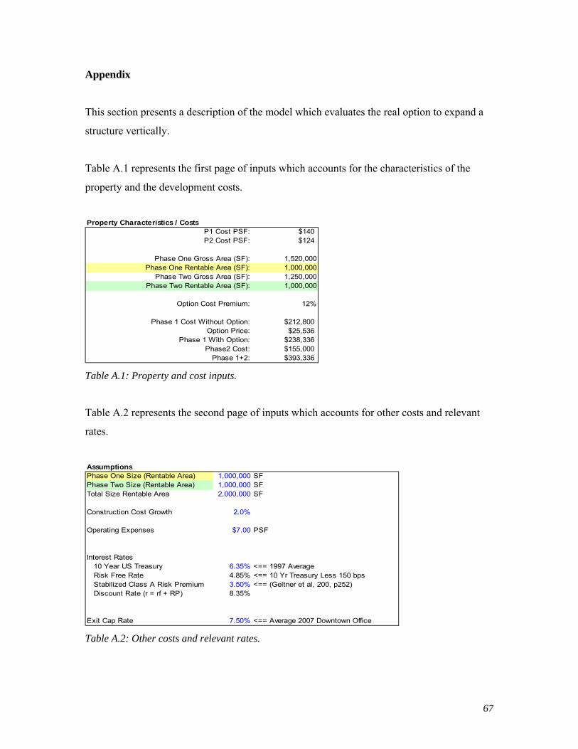
67
Appendix
This section presents a description of the model which evaluates the real option to expand a
structure vertically.
Table A.1 represents the first page of inputs which accounts for the characteristics of the
property and the development costs.
Property Characteristics / Costs
P1 Cost PSF: $140P2 Cost PSF: $124
Phase One Gross Area (SF): 1,520,000Phase One Rentable Area (SF): 1,000,000
Phase Two Gross Area (SF): 1,250,000Phase Two Rentable Area (SF): 1,000,000
Option Cost Premium: 12%
Phase 1 Cost Without Option: $212,800Option Price: $25,536
Phase 1 With Option: $238,336Phase2 Cost: $155,000
Phase 1+2: $393,336 Table A.1: Property and cost inputs.
Table A.2 represents the second page of inputs which accounts for other costs and relevant
rates.
AssumptionsPhase One Size (Rentable Area) 1,000,000 SFPhase Two Size (Rentable Area) 1,000,000 SFTotal Size Rentable Area 2,000,000 SF
Construction Cost Growth 2.0%
Operating Expenses $7.00 PSF
Interest Rates10 Year US Treasury 6.35% <== 1997 AverageRisk Free Rate 4.85% <== 10 Yr Treasury Less 150 bpsStabilized Class A Risk Premium 3.50% <== (Geltner et al, 200, p252)Discount Rate (r = rf + RP) 8.35%
Exit Cap Rate 7.50% <== Average 2007 Downtown Office Table A.2: Other costs and relevant rates.
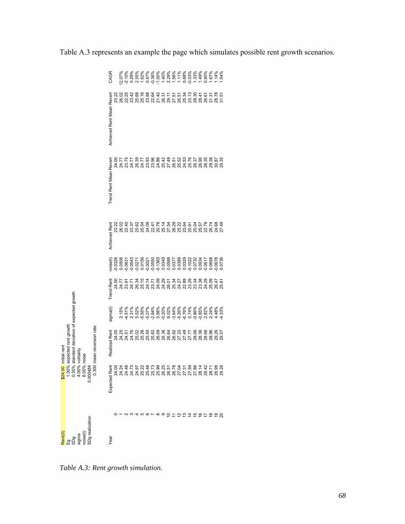
68
Table A.3 represents an example the page which simulates possible rent growth scenarios.
Table A.3: Rent growth simulation.
Ren
t(0)
$24.
00in
itial
rent
Eg1.
00%
expe
cted
rent
gro
wth
SDg
0.35
%st
anda
rd d
evia
tion
of e
xpec
ted
grow
thsi
gma
4.00
%vo
lital
ityno
ise(
t)8.
00%
nois
eSD
g re
aliz
atio
n0.
0004
840.
300
mea
n re
vers
ion
rate
Year
Expe
cted
Ren
tR
ealiz
ed R
ent
sigm
a(t)
Tren
d R
ent
nois
e(t)
Ach
ieve
d R
ent
Tren
d R
ent M
ean
Rev
ert
Achi
eved
Ren
t Mea
n R
ever
tC
AG
R0
24.0
024
.00
24.0
0-0
.032
623
.22
24.0
023
.22
124
.24
24.2
52.
15%
24.7
70.
0506
26.0
224
.77
26.0
212
.07%
224
.48
24.5
1-4
.51%
23.9
1-0
.063
122
.40
23.7
522
.25
-2.1
0%3
24.7
324
.76
2.31
%24
.71
-0.0
543
23.3
724
.77
23.4
20.
29%
424
.97
25.0
25.
52%
26.3
4-0
.027
125
.62
26.3
925
.68
2.55
%5
25.2
225
.28
-5.5
5%25
.15
0.01
5625
.54
24.7
725
.16
1.62
%6
25.4
825
.55
-5.0
7%24
.14
-0.0
021
24.0
923
.93
23.8
80.
47%
725
.73
25.8
2-2
.84%
23.7
1-0
.055
022
.41
23.9
622
.64
-0.3
6%8
25.9
926
.09
0.56
%24
.09
-0.1
383
20.7
624
.86
21.4
2-1
.00%
926
.25
26.3
6-0
.20%
24.2
90.
0349
25.1
425
.42
26.3
11.
40%
1026
.51
26.6
46.
02%
26.0
10.
0588
27.5
427
.49
29.1
12.
29%
1126
.78
26.9
2-3
.64%
25.3
40.
0377
26.2
926
.51
27.5
11.
56%
1227
.04
27.2
0-5
.26%
24.2
70.
0389
25.2
225
.52
26.5
11.
11%
1327
.31
27.4
9-6
.76%
22.8
90.
0329
23.6
424
.53
25.3
40.
68%
1427
.59
27.7
70.
74%
23.2
9-0
.102
220
.91
25.7
623
.13
-0.0
3%15
27.8
628
.06
-0.8
6%23
.34
0.07
3225
.04
26.3
728
.30
1.33
%16
28.1
428
.36
-0.8
5%23
.38
0.09
3425
.57
26.9
029
.41
1.49
%17
28.4
228
.66
2.82
%24
.29
-0.0
617
22.7
928
.35
26.6
10.
80%
1828
.71
28.9
62.
24%
25.0
90.
0658
26.7
429
.38
31.3
11.
67%
1928
.99
29.2
64.
48%
26.4
7-0
.067
824
.68
30.8
728
.78
1.14
%20
29.2
829
.57
-4.3
3%25
.61
0.07
3627
.49
29.3
531
.51
1.54
%

69
Table A.4 represents an example the page which simulates possible lease-up scenarios.
Table A.4: Lease-up simulation.
Year
1 R
ange
:30
.0%
70.0
%S
ubse
quen
t Yea
r Mam
imum
of R
emai
nder
48%
25%
75%
Yea
r1
23
45
67
89
1011
1213
1415
Leas
e-U
p P
er Y
ear
46.6
3%24
.96%
0.03
%13
.57%
6.13
%4.
01%
2.09
%0.
36%
1.06
%0.
55%
0.29
%0.
10%
0.02
%0.
09%
0.05
%53
.37%
28.4
1%28
.38%
14.8
1%8.
68%
4.67
%2.
57%
2.21
%1.
16%
0.60
%0.
32%
0.21
%0.
20%
0.10
%46
.77%
0.09
%97
.21%
41.4
0%46
.24%
44.8
5%13
.94%
99.2
0%68
.51%
91.9
5%32
.58%
8.12
%92
.96%
86.8
6%
Cum
ulat
ive
Occ
upan
cy46
.63%
71.5
9%71
.62%
85.1
9%91
.32%
95.3
3%97
.43%
97.7
9%98
.84%
99.4
0%99
.68%
99.7
9%99
.80%
99.9
0%99
.95%
Vac
ancy
53.3
7%28
.41%
28.3
8%14
.81%
8.68
%4.
67%
2.57
%2.
21%
1.16
%0.
60%
0.32
%0.
21%
0.20
%0.
10%
0.05
%
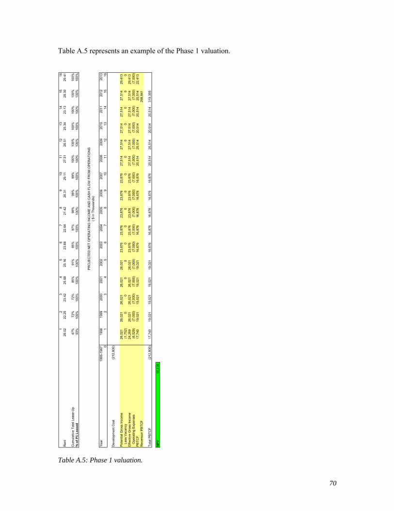
70
Table A.5 represents an example of the Phase 1 valuation.
Table A.5: Phase 1 valuation.
12
34
56
78
910
1112
1314
1516
Ren
t26
.02
22.2
523
.42
25.6
825
.16
23.8
822
.64
21.4
226
.31
29.1
127
.51
26.5
125
.34
23.1
328
.30
29.4
1
Cum
ulat
ive
Tota
l Lea
se-U
p47
%72
%72
%85
%91
%95
%97
%98
%99
%99
%10
0%10
0%10
0%10
0%10
0%10
0%%
of P
1 Le
ased
93%
100%
100%
100%
100%
100%
100%
100%
100%
100%
100%
100%
100%
100%
100%
100%
Year
1995
-199
719
9819
9920
0020
0120
0220
0320
0420
0520
0620
0720
0820
0920
1020
1120
1220
130
12
34
56
78
910
1112
1314
1516
Dev
elop
men
t Cos
t(2
12,8
00)
Pote
ntia
l Gro
ss In
com
e26
,021
26,0
2126
,021
26,0
2126
,021
23,8
7623
,876
23,8
7623
,876
23,8
7627
,514
27,5
1427
,514
27,5
1427
,514
29,4
13Le
ss V
acan
cy(1
,752
)0
00
00
00
00
00
00
00
Effe
ctiv
e G
ross
Inco
me
24,2
6926
,021
26,0
2126
,021
26,0
2123
,876
23,8
7623
,876
23,8
7623
,876
27,5
1427
,514
27,5
1427
,514
27,5
1429
,413
Ope
ratin
g Ex
pens
es(6
,529
)(7
,000
)(7
,000
)(7
,000
)(7
,000
)(7
,000
)(7
,000
)(7
,000
)(7
,000
)(7
,000
)(7
,000
)(7
,000
)(7
,000
)(7
,000
)(7
,000
)(7
,000
)PB
TCF
17,7
4019
,021
19,0
2119
,021
19,0
2116
,876
16,8
7616
,876
16,8
7616
,876
20,5
1420
,514
20,5
1420
,514
20,5
1422
,413
Rev
ersi
on P
BTC
F29
8,84
1
Tota
l PBT
CF
(212
,800
)17
,740
19,0
2119
,021
19,0
2119
,021
16,8
7616
,876
16,8
7616
,876
16,8
7620
,514
20,5
1420
,514
20,5
1431
9,35
5
NPV
32,1
16
PRO
JEC
TED
NET
OPE
RA
TIN
G IN
CO
ME
AND
CAS
H F
LOW
FR
OM
OP
ERAT
ION
S( $
in T
hous
ands
)
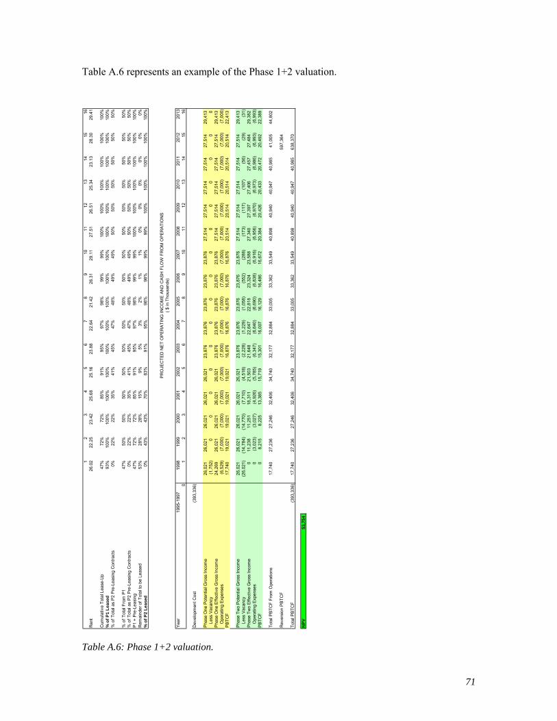
71
Table A.6 represents an example of the Phase 1+2 valuation.
Table A.6: Phase 1+2 valuation.
12
34
56
78
910
1112
1314
1516
Ren
t26
.02
22.2
523
.42
25.6
825
.16
23.8
822
.64
21.4
226
.31
29.1
127
.51
26.5
125
.34
23.1
328
.30
29.4
1
Cum
ulat
ive
Tota
l Lea
se-U
p47
%72
%72
%85
%91
%95
%97
%98
%99
%99
%10
0%10
0%10
0%10
0%10
0%10
0%%
of P
1 Le
ased
93%
100%
100%
100%
100%
100%
100%
100%
100%
100%
100%
100%
100%
100%
100%
100%
% o
f Tot
al a
s P
2 P
re-L
easi
ng C
ontra
cts
0%22
%22
%35
%41
%45
%47
%48
%49
%49
%50
%50
%50
%50
%50
%50
%
% o
f Tot
al F
rom
P1
47%
50%
50%
50%
50%
50%
50%
50%
50%
50%
50%
50%
50%
50%
50%
50%
% o
f Tot
al a
s P
2 P
re-L
easi
ng C
ontra
cts
0%22
%22
%35
%41
%45
%47
%48
%49
%49
%50
%50
%50
%50
%50
%50
%P
1 +
Pre
-Lea
sing
47%
72%
72%
85%
91%
95%
97%
98%
99%
99%
100%
100%
100%
100%
100%
100%
Rem
aind
er o
f Tot
al to
be
Leas
ed53
%28
%28
%15
%9%
5%3%
2%1%
1%0%
0%0%
0%0%
0%%
of P
2 Le
ased
0%43
%43
%70
%83
%91
%95
%96
%98
%99
%99
%10
0%10
0%10
0%10
0%10
0%
Yea
r19
95-1
997
1998
1999
2000
2001
2002
2003
2004
2005
2006
2007
2008
2009
2010
2011
2012
2013
01
23
45
67
89
1011
1213
1415
16
Dev
elop
men
t Cos
t(3
93,3
36)
Pha
se O
ne P
oten
tial G
ross
Inco
me
26,0
2126
,021
26,0
2126
,021
26,0
2123
,876
23,8
7623
,876
23,8
7623
,876
27,5
1427
,514
27,5
1427
,514
27,5
1429
,413
Less
Vac
ancy
(1,7
52)
00
00
00
00
00
00
00
0P
hase
One
Effe
ctiv
e G
ross
Inco
me
24,2
6926
,021
26,0
2126
,021
26,0
2123
,876
23,8
7623
,876
23,8
7623
,876
27,5
1427
,514
27,5
1427
,514
27,5
1429
,413
Ope
ratin
g E
xpen
ses
(6,5
29)
(7,0
00)
(7,0
00)
(7,0
00)
(7,0
00)
(7,0
00)
(7,0
00)
(7,0
00)
(7,0
00)
(7,0
00)
(7,0
00)
(7,0
00)
(7,0
00)
(7,0
00)
(7,0
00)
(7,0
00)
PB
TCF
17,7
4019
,021
19,0
2119
,021
19,0
2116
,876
16,8
7616
,876
16,8
7616
,876
20,5
1420
,514
20,5
1420
,514
20,5
1422
,413
Pha
se T
wo
Pot
entia
l Gro
ss In
com
e26
,021
26,0
2126
,021
26,0
2126
,021
23,8
7623
,876
23,8
7623
,876
23,8
7627
,514
27,5
1427
,514
27,5
1427
,514
29,4
13Le
ss V
acan
cy(2
6,02
1)(1
4,78
4)(1
4,77
0)(7
,710
)(4
,518
)(2
,228
)(1
,229
)(1
,058
)(5
52)
(288
)(1
73)
(117
)(1
07)
(56)
(29)
(31)
Pha
se T
wo
Effe
ctiv
e G
ross
Inco
me
011
,238
11,2
5118
,311
21,5
0321
,648
22,6
4722
,818
23,3
2423
,588
27,3
4027
,397
27,4
0627
,457
27,4
8429
,382
Ope
ratin
g E
xpen
ses
0(3
,023
)(3
,027
)(4
,926
)(5
,785
)(6
,347
)(6
,640
)(6
,690
)(6
,838
)(6
,916
)(6
,956
)(6
,970
)(6
,973
)(6
,986
)(6
,993
)(6
,993
)P
BTC
F0
8,21
58,
225
13,3
8515
,719
15,3
0116
,007
16,1
2916
,486
16,6
7220
,384
20,4
2620
,433
20,4
7220
,492
22,3
89
Tota
l PB
TCF
From
Ope
ratio
ns17
,740
27,2
3627
,246
32,4
0634
,740
32,1
7732
,884
33,0
0533
,362
33,5
4940
,898
40,9
4040
,947
40,9
8541
,005
44,8
02
Rev
ersi
on P
BTC
F59
7,36
4
Tota
l PB
TCF
(393
,336
)17
,740
27,2
3627
,246
32,4
0634
,740
32,1
7732
,884
33,0
0533
,362
33,5
4940
,898
40,9
4040
,947
40,9
8563
8,37
0
NPV
53,7
54
PR
OJE
CTE
D N
ET O
PE
RA
TIN
G IN
CO
ME
AN
D C
ASH
FLO
W F
RO
M O
PE
RA
TIO
NS
( $ in
Tho
usan
ds)

72
Table A.7 represents an example of the Flexible scenario exercise decision and valuation.
Table A.7: Flexible case valuation.
12
34
56
78
910
1112
1314
1516
Ren
t26
.54
24.2
021
.68
24.2
126
.49
29.3
128
.97
27.2
028
.26
25.3
929
.08
24.3
924
.60
31.3
428
.51
27.4
327
.44
Cum
ulat
ive
Tota
l Lea
se-U
p46
%81
%93
%95
%98
%99
%10
0%10
0%10
0%10
0%10
0%10
0%10
0%10
0%10
0%10
0%%
of P
1 Le
ased
92%
100%
100%
100%
100%
100%
100%
100%
100%
100%
100%
100%
100%
100%
100%
100%
% o
f Tot
al a
s P2
Pre
-Lea
sing
Con
tract
s0%
31%
43%
45%
48%
49%
50%
50%
50%
50%
50%
50%
50%
50%
50%
50%
% o
f Tot
al F
rom
P1
46%
50%
50%
50%
50%
50%
50%
50%
50%
50%
50%
50%
50%
50%
50%
50%
% o
f Tot
al a
s P2
Pre
-Lea
sing
Con
tract
s0%
31%
43%
45%
48%
49%
50%
50%
50%
50%
50%
50%
50%
50%
50%
50%
P1
+ P
re-L
easi
ng46
%81
%93
%95
%98
%99
%10
0%10
0%10
0%10
0%10
0%10
0%10
0%10
0%10
0%10
0%R
emai
nder
of T
otal
to b
e Le
ased
54%
19%
7%5%
2%1%
0%0%
0%0%
0%0%
0%0%
0%0%
% o
f P2
Pre-
Leas
ed0%
61%
86%
91%
97%
99%
99%
100%
100%
100%
100%
100%
100%
100%
100%
100%
Yea
r19
95-1
997
1998
1999
2000
2001
2002
2003
2004
2005
2006
2007
2008
2009
2010
2011
2012
2013
01
23
45
67
89
1011
1213
1415
16
Pha
se 1
Dev
elop
men
t Cos
t(2
38,3
36)
Pha
se O
ne P
oten
tial G
ross
Inco
me
24,2
0424
,204
24,2
0424
,204
24,2
0428
,972
28,9
7228
,972
28,9
7228
,972
24,3
9524
,395
24,3
9524
,395
24,3
9527
,443
Less
Vac
ancy
(1,8
23)
00
00
00
00
00
00
00
0P
hase
One
Effe
ctiv
e G
ross
Inco
me
22,3
8224
,204
24,2
0424
,204
24,2
0428
,972
28,9
7228
,972
28,9
7228
,972
24,3
9524
,395
24,3
9524
,395
24,3
9527
,443
Ope
ratin
g Ex
pens
es(6
,473
)(7
,000
)(7
,000
)(7
,000
)(7
,000
)(7
,000
)(7
,000
)(7
,000
)(7
,000
)(7
,000
)(7
,000
)(7
,000
)(7
,000
)(7
,000
)(7
,000
)(7
,000
)P
BTC
F15
,909
17,2
0417
,204
17,2
0417
,204
21,9
7221
,972
21,9
7221
,972
21,9
7217
,395
17,3
9517
,395
17,3
9517
,395
20,4
43
Pha
se 2
Dev
elop
men
t Cos
t(1
55,0
00)
(158
,100
)(1
61,2
62)
(164
,487
)(1
67,7
77)
(171
,133
)(1
74,5
55)
(178
,046
)(1
81,6
07)
(185
,239
)(1
88,9
44)
(192
,723
)(1
96,5
77)
(200
,509
)(2
04,5
19)
(208
,610
)(2
12,7
82)
Exe
rcis
e O
ptio
nN
ON
ON
ON
OY
ESY
ESN
ON
ON
ON
ON
ON
OYE
SN
O"Y
ES" C
ount
33
33
32
11
11
11
10
Pha
se T
wo
Pote
ntia
l Gro
ss In
com
e0
00
027
,196
28,2
6027
,196
27,1
9627
,196
24,5
9724
,597
24,5
9724
,597
24,5
97Le
ss V
acan
cy0
00
0(2
10)
(79)
(55)
(51)
(18)
(15)
(14)
(5)
(3)
(3)
Pha
se T
wo
Effe
ctiv
e G
ross
Inco
me
00
00
26,9
8628
,182
27,1
4127
,145
27,1
7724
,583
24,5
8324
,592
24,5
9424
,594
Ope
ratin
g Ex
pens
es0
00
0(6
,946
)(6
,981
)(6
,986
)(6
,987
)(6
,995
)(6
,996
)(6
,996
)(6
,999
)(6
,999
)(6
,999
)P
BTC
F0
00
020
,040
21,2
0120
,155
20,1
5820
,182
17,5
8717
,587
17,5
9417
,595
17,5
95
PBT
CF
From
Ope
ratio
ns15
,909
17,2
0417
,204
17,2
0417
,204
21,9
7242
,012
43,1
7342
,127
42,1
3037
,577
34,9
8234
,982
34,9
8834
,990
38,0
38R
ever
sion
PB
TCF
507,
172
Dev
elop
men
t Cos
ts(2
38,3
36)
00
00
(171
,133
)0
00
00
00
0
Tota
l PBT
CF
15,9
0917
,204
17,2
0417
,204
17,2
0421
,972
42,0
1243
,173
42,1
2742
,130
37,5
7734
,982
34,9
8234
,988
542,
162
PV
of D
evel
opm
ent C
osts
(352
,937
)Ph
ase
2 C
ost
(171
,133
)P
V of
Pro
perty
381,
951
NPV
29,0
14
Ren
t Gro
wth
Hur
dle:
1.0%
Ren
t CA
GR
:-8
.8%
-9.6
%-3
.0%
0.0%
2.0%
1.5%
0.4%
0.8%
-0.5
%0.
9%-0
.8%
-0.6
%1.
3%0.
5%P
2 Pr
e-Le
asin
g H
urdl
e:93
.0%
% o
f P2
Pre
-Lea
sed:
0.0%
61.2
%86
.0%
90.6
%96
.6%
98.8
%99
.2%
99.7
%99
.8%
99.8
%99
.9%
99.9
%99
.9%
100.
0%
NO
NO
NO
NO
YES
YES
NO
NO
NO
NO
NO
NO
YES
NO
00
00
50
00
00
00
00
Exer
cise
Yea
r5
PRO
JEC
TED
NE
T O
PER
ATIN
G IN
CO
ME
AN
D C
ASH
FLO
W F
RO
M O
PER
ATI
ON
S( $
in T
hous
ands
)