Policy Research Working Paper 5096

Missing Women and India’s Religious Demography

Vani BorooahQuy-Toan Do

Sriya Iyer Shareen Joshi

The World BankDevelopment Research GroupPoverty and Inequality TeamOctober 2009

WPS5096

Produced by the Research Support Team

Abstract

The Policy Research Working Paper Series disseminates the findings of work in progress to encourage the exchange of ideas about development issues. An objective of the series is to get the findings out quickly, even if the presentations are less than fully polished. The papers carry the names of the authors and should be cited accordingly. The findings, interpretations, and conclusions expressed in this paper are entirely those of the authors. They do not necessarily represent the views of the International Bank for Reconstruction and Development/World Bank and its affiliated organizations, or those of the Executive Directors of the World Bank or the governments they represent.

Policy Research Working Paper 5096

The authors use recent data from the 2006 National Family Health Survey of India to explore the relationship between religion and demographic behavior. They find that fertility and mortality vary not only between religious groups, but also across caste groups. These groups also differ with respect to socio-economic status. The central finding of this paper is that despite their socio-economic disadvantages, Muslims have higher fertility than their Hindu counterparts and also exhibit

This paper—a product of the Poverty and Inequality Team, Development Research Group—is part of a larger effort in the department to understand the relations between religion and demography. Policy Research Working Papers are also posted on the Web at http://econ.worldbank.org. The author may be contacted at pflewitt@worldbank.org.

lower levels of infant mortality (particularly female infant mortality). This effect is robust to the inclusion of controls for non-religious factors such as socio-economic status and area of residence. This result has important policy implications because it suggests that India's problem of “missing women” may be concentrated in particular groups. The authors conclude that religion and caste play a key role in determining the demographic characteristics of India.

Missing Women and India’s Religious Demography∗

Vani Borooah† Quy-Toan Do‡ Sriya Iyer§ Shareen Joshi¶

1 Introduction

Two features of India’s demography have recently received a great deal of attention. The

first is gender bias - the small number of females compared to males (Visaria, 1971; Dyson

and Moore, 1983; Sen, 1992, 2001; Kishor, 1993; Das Gupta, 2005). According to the 2001

Census, India has 933 females for every 1000 males, which implies that as many as 35–37

million women in India may be “missing” (Dreze and Sen, 1996; Klasen, 1994; Agnihotri,

2000; Sen, 2003; Oster, 2005).1 The second feature is that demographic variables in India

vary sharply by religious group. Fertility and the population growth rate for example,

are higher among Muslims than Hindus (Basu 1997; Jeffery and Jeffery 1997; Iyer 2002;

Dharmalingam and Morgan, 2004).2

In the literature on Indian demography, both these issues have received enormous at-

tention, but they have typically been studied independently of each other. The adverse sex

∗For helpful discussions we are grateful to Robert Barro, Eli Berman, Edward Glaeser, Timothy Guinnane,Monica Das Gupta, Partha Dasgupta, Larry Iannaccone, Siddiq Osmani, Abusaleh Shariff, Chander Velu,David Voas, and to participants at the American Economic Association 2007 meetings in Chicago, the‘Religion, Economics and Culture’ 2004 Annual Meetings in Kansas City, Missouri, and the 2005 ESRCseminar on ‘Demography and Religion’ in Lancaster, UK. We are also grateful to Sarina Siddhanti forexcellent research assistance, We are especially grateful to the Editor and two anonymous referees for theirinvaluable comments.†Faculty of Economics and Politics, University of Ulster, Northern Ireland. vk.borooah@ulst.ac.uk‡Development Economics Research Group, The World Bank. qdo@worldbank.org§Corresponding author: Faculty of Economics and St. Catharine’s College, University of Cambridge,

Sidgwick Avenue, Cambridge CB3 9DD, United Kingdom. Tel: 44 1223 335257; Fax: 44 1223 335475;Email: Sriya.Iyer@econ.cam.ac.uk¶The School of Foreign Service, Georgetown University. shareen.joshi@gmail.com1The estimate of the number of missing women is based on comparisons with Europe and North America

which have 1050 females per 1000 males.2An often-cited figure from the National Family Health Survey conducted in 1998-99, shows that the

Total Fertility Rate (TFR) for Hindus and Muslims was 2.8 and 3.6 respectively.

1

ratio is mainly discussed in the context of the preference that many South and East Asian

families have for sons over daughters (‘son preference’) and related issues that concern the

marriage market, fertility, and dowry (Edlund, 1999; Bhat and Zavier, 2003; Sen, 2001;

Rao, 1993; Bloch and Rao, 2002; Botticini and Siow, 2003; Das Gupta, 2005; Jacoby and

Mansuri, 2006). The demographic differences between Hindus and Muslims, on the other

hand, have usually been discussed in terms of the number of children in Muslim families

and the higher population growth rates of this community. However, the debate often over-

looked the fact that infant mortality among Muslims (at 59 per 1000) is much lower than

that among Hindus (at 77 per 1000) as documented in Borooah and Iyer (2005a). Similarly

child mortality, which is 83 per 1000 for Muslims, is substantially lower than child mortality

among Hindus, at 107 per 1000 (IIPS and ORC Macro International, 2000). The survival

advantage of Muslim children despite the higher fertility of their mothers is particularly

puzzling in light of the fact that Muslims in India are typically poorer than Hindus as

highlighted by the Sachar Committee Report (Government of India, 2006). Even a cursory

glance at these facts and figures suggests that religious differentials in infant mortality need

to be examined more closely.

In this paper, we link these two separately-studied demographic realities into a com-

parative analysis of infant mortality across religious and caste groups, using data from the

newly released National Family Health Survey of 2005-06. To do so, we first divide our

population into three subgroups: non-Dalit Hindus (also known as upper-caste Hindus),

Dalit Hindus (also known as lower-caste Hindus), and Muslims. Our preliminary compara-

tive analysis finds that with respect to observable socio-economic characteristics, Muslims

are similar to Hindu Dalits in that they have lower levels of education, are poorer than

non-Dalit Hindus. They also have more children, are less likely to experience the death of

a child (particularly a girl), have higher female-male sex ratios among children alive as well

as among children ever-born, are less likely to use contraception, and have preferences for a

greater number of girls as well as boys. The next step of our analysis is to estimate survival

probabilities for children and control for a number of important socio-economic, geographic

and demographic variables. Our findings confirm that Muslim infant and child mortality

is considerably lower than that for the Hindus, even after accounting for the wide range

of socio-economic characteristics available to us. The effect is particularly strong for girls.

Female infant mortality rates are lower in Muslim families than in Hindu families even with

the inclusion of numerous controls for household and community characteristics. The final

2

step of our analysis involves a series of robustness checks. We find that our results are

upheld. Although we cannot rule out all possible alternative rationales, or the possibility

that socio-economic status may be insufficiently captured by our controls, these results lend

support to the conjecture that religion might play a direct role in explaining the differences

in gender differences in mortality between the Hindus and Muslims of India.

This paper proceeds as follows: Section 2 discusses the role of religion in Indian demog-

raphy and establishes our conjecture; Section 3 conducts a comparative analysis of non-Dalit

Hindus, Dalit Hindus and Muslims. Section 4 concludes.

2 The Role of Religion in Indian Demography

The idea that religion can shape demographic behavior is not new, particularly in the con-

text of South Asia. Most of the existing literature on religion and demography however,

focuses on fertility alone. Two main theories have dominated the discussion of religious

differences in Indian fertility rates. The ‘characteristics hypothesis’ proposes that the rel-

ative poverty and lower education levels of Muslims drive fertility and mortality patterns

that are different than those observed among Hindus (Iyer, 2002). In contrast to this, the

‘particularized theology hypothesis’ - or the ’pure religion effect’ argues that the intellec-

tual content of religion affects fertility directly. Proponents of this hypothesis point out

that religious injunctions in favor of multiple wives, large numbers of children, and a ban

on the use of contraception and abortion may encourage higher fertility among Muslims.

Such arguments however, have also been made for Hindus. The Mysore Population Study

conducted in 1961, for example, concluded that Hindu religious traditions in Indian society

favored having many offspring (United Nations, 1961).

We believe that the focus on fertility, to the exclusion of other demographic variables

such as mortality and the sex-composition of off-spring, is incomplete. For the remainder of

this section, we document the differences in beliefs and norms between Hindus and Muslims

that may impact their perceived benefits of sons versus daughters.

In Islam, the institutional requirements of the religion are specified in the Sharia or

Islamic law which is derived from two main sources – the Koran and the Sunnah, and also

the writings of the medieval theologian Al Ghazzali, often cited by Muslim clerics, who

3

summarized Sunni and Shia positions on demography-related issues such as marriage and

birth control (Al Ghazzali, 1909).3 In the case of Hinduism we consider religious texts

such as Vedas, and Upanishads (Radhakrishnan, 1923); epic poems such as the Ramayana

and Mahabharata (Deshpande, 1978); social commentaries such as Kautilya’s Arthasastra

(Shamasastry, 1951); and verse-poems in praise of Hindu goddesses such as the Lalita-

sahasranama and the Sri-sukta (Suryanaraya Murthy, 2000) in the context of Indian de-

mography (see Iyer, 2002 for a more detailed discussion of this literature).

A close and comparative reading of the above texts suggests that the costs and benefits

of sons compared to daughters may be different within Islam compared to Hinduism. While

both religions encourage marriage, the nature of the contract differs. An Islamic marriage

or the nikah, is defined not really as a sacrament, but more as a civil contract (Azim,

1997).4 Parents and guardians exercise control over the selection of marriage partners,

and a dower or ‘bride price’ is paid to the bride or her guardian (Youssef, 1978, p.78).

The Koran recognizes the possibility of divorce and encourages remarriage of divorced or

widowed women (Qureshi, 1980: 564; Youssef, 1978: 88, Coulson and Hinchcliffe, 1978:

37-38). In the context of India, this is important for Muslim families as the investments in

daughters are frequently recoverable after marriage.

As in Islam, Hinduism also encourages all Hindus to enter married life.5 The marriage of

a daughter for Hindus is described as kanyadaan – this can be translated as the ‘donation’

of a daughter. Such a donation is believed to benefit Hindu families both socially and

religiously (Niraula and Morgan, 1996). Once married, women cease to be members of

their natal home, and are generally not permitted to remarry in the event of divorce or

widowhood. Hindu marriages are often accompanied by the giving and taking of significant

dowries, i.e. payments from the family of the bride to the groom (Edlund, 1999; Bhat and

Zavier, 2003; Rao, 1993; Bloch and Rao, 2002; Botticini and Siow, 2003). Women do not

have property rights over these dowries and they are not returned to her or her family in

the event of divorce or widowhood.

3The Sunnah are the interpretations of the words of Mohammad and their application to various situa-tions.

4For a Muslim marriage to be legally valid, it needs to meet four conditions: proposal by one party;acceptance by the other; the presence of a sufficient number of witnesses (two in Sunni law); and a formalexpression of both the proposal and the acceptance at the same meeting (Azim 1997).

5For example Shakuntala, a princess from Hindu mythology tells Dushyanta her beloved that ‘when a hus-band and wife are carrying on smoothly, then only pleasure, prosperity and piety are possible’ (Deshpande,1978: 91).

4

Such distinctions between the ‘contractual’ versus the ‘donational’ notion of marriage

in Islam compared to Hinduism have implications for the relative costs and benefits of

having sons and daughters. From a purely economic perspective, the net benefit of having

daughters may be more ‘costly’ for Hindu than for Muslim parents in India. Investments

in daughters are also not recoverable.

The preference for sons over daughters is also emphasized by other areas of Hindu ritual

and philosophy. For example, securing a good ‘rebirth’ is believed to be directly related

to whether the eldest son of a deceased individual lights the funeral pyre. This sentiment

is echoed in many writings: ‘At the end of the (Sraddha) death ceremony the performer

asks, “Let me, O fathers, have a hero for a son!”’ (Radhakrishnan, 1927, pp. 59-60).

Additionally, sons are believed to be a vital source of security in old-age. Daughters are

generally considered to ‘belong’ to the family that they marry into, and so cannot be viewed

as a source of support to her natal family.

It must be emphasized that son-preference has also been documented in Islamic society.

Islamic law is patriarchal and patrilineal. Sons are given twice as large an inheritance as

daughters are and a man’s testimony in court is worth twice that of a woman (Coulson and

Hinchcliffe, 1978). Women in Islamic societies have typically been restricted to a lifestyle

that guaranteed preservation of family honor and prestige and had limited opportunities

to participate in labor markets (Coulson and Hinchcliffe, 1978: 38; Obermeyer, 1992). We

simply argue that son-preference may less unequivocal as it is with Hindus. More recently,

some sociological evidence has also emphasized this. For example, in his study of 378

Muslim women and men in Mangalore, Azim found that over two-third of respondents in

his sample did not prefer sons, over daughters (Azim, 1997, p. 187); moreover, a large

proportion of those who did were from poor and illiterate households (Azim, 1997: 189).

Other nationally representative data from the National Family Health Surveys of India also

show that about one-third of Muslims do not prefer sons over daughters (Kishor, 1993). 6

The relative importance of sons and daughters may stem not only from theology, but

also from the differential socio-economic circumstances of Hindus and Muslims (Iyer, 2002;

6An early example of the recognition of the contrast in gender norms comes from Maulana Ashraf AliThanavi who wrote a compendium of useful knowledge for women. He condemned the practice of blessing awoman by wishing her husband, brother, or children long life, or wishing for her many sons and grandsons(Minault 1998, p. 62). He argued that this was not suficiently Islamic because to view women blessed interms of their relation to men and sons devalues their relationship to God, and hence goes against the tenetthat all are equal in his sight.

5

Dharmalingam and Morgan, 2004). For example, in India today, it seems important to

have educated sons, but in order to get daughters married, it is equally important to have

educated daughters. If the average levels of education among Muslim men are for example

lower than among Hindu men, then there may be lower educational investments also required

of Muslim women (Borooah and Iyer, 2005b). A related issue is land ownership – there

may be a greater desire on the part of Hindus to have sons in order to keep land within the

patrilineal family line. It is documented that land ownership among Muslims is less than

among Hindus (Shariff, 1999). In summary, for reasons that stem both from theological

considerations, and from the socio-economic characteristics of religious groups, there may

be important differences between Hindus and Muslims in their fertility and mortality of

sons compared to daughters. We next turn to a formal investigation of the socio-economic

determinants of fertility and mortality differences between Hindus and Muslims.

3 Fertility, Mortality and Religion in India

India today has a total population of just over 1.1 billion people. Census data shows that

Hindus form over 80 percent of India’s population, while Muslims form approximately 15

percent. Muslims are the most significant ‘minority’ population and consist of approxi-

mately 150 million people. Our description of contemporary India uses data from the newly

released 2005-06 National Family Health Survey (NFHS-3).7 The NFHS interviewed a total

of 123,385 women in 29 states of India. The survey is based on a sample of housesholds

that is representative at the state as well as national level. The religious composition of

the households is consistent with the findings of the Indian Census (2001): 82 percent of

households are Hindu, 13 percent are Muslim, 3 percent are Christian, 2 percent are Sikh,

and the remainder are other religions. Among Hindus, the caste composition of our popu-

lation also mirrors the census. 44% of Hindu respondents reported that they belonged to

a “Scheduled Caste” or a “Scheduled Tribe” (henceforth referred to as Dalits), and 44% of

7The first NFHS survey was conducted in 1992-93, and the second in 1998-99. All three surveys wereconducted in conjunction with the Ministry of Health and Family Welfare (MOHFW),Government of India.Funding for the survey was provided by the United States Agency for International Development (US-AID), the United Kingdom Department for International Development (DFID), the Bill and Melinda GatesFoundation, UNICEF, UNFPA, and the government of India. Technical assistance was provided by MacroInternational Maryland, USA.

6

the Hindu population was higher caste or non-Dalit.8

We restrict our sample by including only those households that are Hindu and Muslim,

and in which at least one female respondent had borne children. This leaves us with a sample

of a total of 81,021 women. Panel A of Table 1 presents additional summary statistics for

the female sample.

The basis of our analysis is a comparison between the demographic and socio-economic

differences between three subgroups of India’s population: the Dalits, Muslims, and Hin-

dus. Since these categories are conceptually overlapping, we define three mutually exlusive

categories: non-Dalit Hindus; Muslims; and Dalit Hindus.9

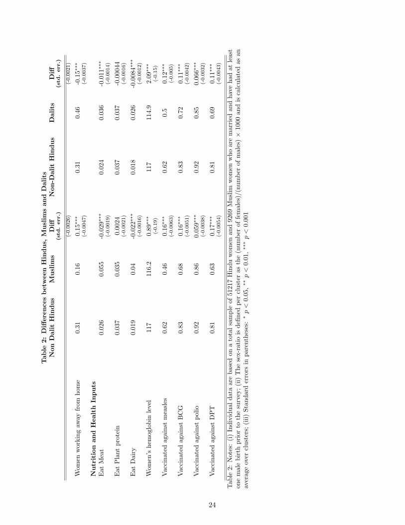
We begin with a comparison of socio-economic variables for the three groups in our

sample. The first three columns of Table 2 explore differences between non-Dalit Hindus

and Muslims, and the next three columns explore differences between non-Dalit and Dalit

Hindus. Note that in nearly all respects, non-Dalit Hindus appear richer than Muslims

and their Dalit counterparts. They also have higher rates of schooling, lower fertility,

higher ownership of farmland and a lower chance of falling below the poverty line. In other

words, Muslims and Dalits both appear to be socio-economically disadvantaged relative

to upper-caste Hindus. The differences are statistically significant. Where Hindu Dalits

and Muslims diverge from each other significantly is in the rates of female labor-force

participation. Muslim women work less than their non-Dalit Hindu counterparts, while

Dalit Hindus work more. The differences are also visible in other indicators of female labor

force participation rates. Muslim women (Dalit women) are less (more) likely to be self-

employed, and less (more) likely to work away from home. These differences are again

statistically significant.

While Muslims are similar to Dalit Hindus on a range of socio-economic characteristics,

8The term ’Dalit’ translates as ’the downtrodden’, and refers specifically to India’s Scheduled Castesand Sceduled Tribes - these are those castes and tribes recognised by the Indian Constitution as deservingspecial recognition in respect of education, job reservation in employment, and political representation.

9While Dalits are also found among Muslims in India (Sachar Committee Report, 2006), we restrict ourattention to the Hindu Dalits. This is for two reasons. First, while 30% of Hindus are Dalits, the proportionof Muslims reporting Dalit-status is approximately 2–5% (Sachar Committee Report, 2006). Second, amongHindus, the criteria for being a Dalit are widely recognized. As mentioned in the footnote above, the Indiangovernment maintains official lists of “scheduled castes” and “scheduled tribes”. Such benchmarks do not yetexist among other groups, making the categorization of particular houses in a survey somewhat subjective.In our sample, only 452 Muslim women reported themselves as Dalits. We included this group in our Muslimsample, but excluded them from the Dalit sample.

7

they appear to be quite similar to upper-caste Hindus in that they are less likely to expe-

rience the death of a child (particularly a girl), have higher female-male sex ratios among

children alive as well as among children ever-born, are less likely to use contraception and

have preferences for greater number of girls as well as boys, as evidenced by the greater

numbers of girls and boys that they regard as “ideal”.10,11 In all these cases, the differences

are statistically significant. Age-specific fertility also confirms that Muslim women bear

larger numbers of children at earlier ages than women from other religious groups (Figure

1).

3.1 Fertility Differences

To explore the often-cited fact about higher Muslim fertility, we construct from the female

sample the total number of children the woman has had (those born alive as well as those who

have died, but excluding miscarriages and stillborns). We first examine the determinants of

fertility on the entire sample of women, and then restrict the sample to women over the ages

of 30 and 40. Estimation on the restricted sample permits us to examine the relationships

for women who have most likely completed their child-bearing.

We control for a variety of other individual, family and regional characteristics. First,

we control for a woman’s age because of the well-known fact that children born to mothers

at very young or very old ages are more likely to die in infancy than children born to

mothers in prime childbearing ages. A second set of controls includes variables on whether

a woman (the child’s mother) and her husband (the child’s father) had completed primary

school. We also include a dummy variable indicating whether they had never attended

school. Third, we control for economic status using a wealth index. This index has been

developed and tested in a large number of countries and has been shown to be consistent

10Sex-ratios are measured at the level of the cluster/village rather than at the level of a woman. Sincea sex-ratio is defined as the number of females relative to the number of males, it can only be constructedfor a woman who has had at least one male birth. When aggregating at the level of the village or cluster(which was the NFHS primary sampling unit) however, this problem is alleviated, since it is an average offemale and male deaths for a broad group of women.

11The low female-male ratio at birth may be attributed to the fact that the practice of sex selective abortionis higher among upper-caste Hindus. This group has been shown to engage in this practice more than othergroups (Arnold, Kishor and Roy, 2002). However, since the NFHS data do not contain information on theprevalence and practice of abortion, this is one aspect that we are not able to investigate comprehensively.However, we do acknowledge, readily, the importance of these practices for the subject of this research.

8

with expenditure and income measures (Rustein, 1999; Filmer and Pritchett, 2001).12 We

also include a control for whether the family resides in a rural area. Rural areas in India

typically have significantly higher rates of infant mortality than urban areas. We finally add

dummy variables for states and the region in which an individual resides. This is intended

to capture state- or region-fixed effects.

The results of the fertility regression are presented in Table 3. As expected, and based

on the summary statistics seen in Table 2, the coefficients for Muslim and Hindu Non-Dalit

take opposite signs: Muslims have more children, and Hindu Non-Dalits have fewer children

than the omitted group (Dalits) and these differences remain statistically significant even

when all the control variables are included. Muslims have about 1 child more than Dalits and

Non-Dalits have about 0.3 fewer children than Dalits. We interepret this as evidence that

Muslim fertility is higher than Hindu fertility overall. Additionally, most measures of socio-

economic status have the expected negative sign in the fertility regressions. The household

wealth index as well as parental age and education are all associated with decreased fertility.

As widely seen in the empirical literature, maternal attributes have a stronger effect on

fertility than paternal attributes.

In results not shown here, we examine the robustness of the relationship between religion

and fertility by employing additional socio-economic and demographic variables such as the

use of contraception (traditional as well as modern), duration of the use of contraception,

exposure to mass media and nutritional indicators. Inclusion of these additional explanatory

variables had little to no effect on the two variables Muslim and Hindu Non-Dalit that are

central to our interest in this paper.

12The wealth index is constructed by combining information on 33 household assets and housing charac-teristics such as ownership of consumer items, type of dwelling, source of water, and availability of electricityinto a single wealth index. These 33 assets are as follows: household electrification, type of windows, drink-ing water source, type of toilet facility, type of flooring, material of exterior walls, type of roofing, cookingfuel, house ownership, number of household members per sleeping room, ownership of a bank account, own-ership of a mattress, a pressure cooker, a chair, a cot/bed, a table, an electric fan, a radio/transmitter, ablack and white television, a color television, a sewing machine, a mobile phone, another other telephone, acomputer, a refrigerator, a watch or clock, a bicycle, a motorcycle or scooter, an animal-drawn cart, a car,a water-pump, a thresher, and a tractor. Each household asset is assigned a weight (factor score) that isgenerated through principal components analysis. The resulting asset scores are standardized in relation toa normal household and is then assigned a score for each asset, and scores were summed for each household;individuals are ranked according to the score of the household in which they reside.

9

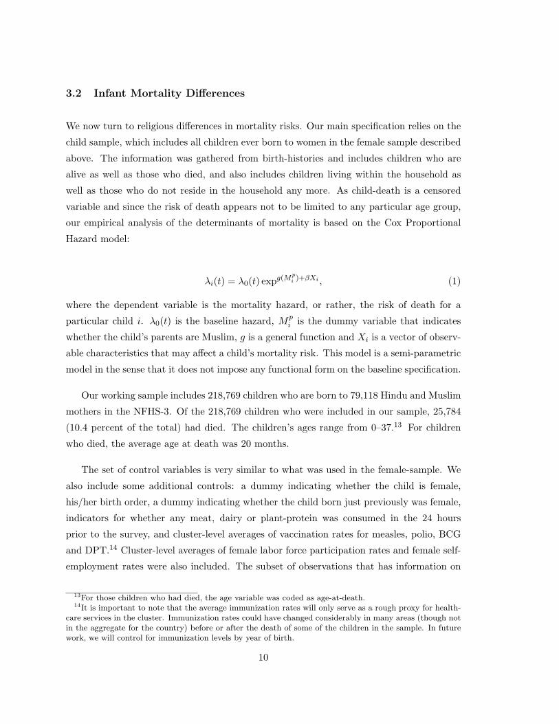
3.2 Infant Mortality Differences

We now turn to religious differences in mortality risks. Our main specification relies on the

child sample, which includes all children ever born to women in the female sample described

above. The information was gathered from birth-histories and includes children who are

alive as well as those who died, and also includes children living within the household as

well as those who do not reside in the household any more. As child-death is a censored

variable and since the risk of death appears not to be limited to any particular age group,

our empirical analysis of the determinants of mortality is based on the Cox Proportional

Hazard model:

λi(t) = λ0(t) expg(Mpi )+βXi , (1)

where the dependent variable is the mortality hazard, or rather, the risk of death for a

particular child i. λ0(t) is the baseline hazard, Mpi is the dummy variable that indicates

whether the child’s parents are Muslim, g is a general function and Xi is a vector of observ-

able characteristics that may affect a child’s mortality risk. This model is a semi-parametric

model in the sense that it does not impose any functional form on the baseline specification.

Our working sample includes 218,769 children who are born to 79,118 Hindu and Muslim

mothers in the NFHS-3. Of the 218,769 children who were included in our sample, 25,784

(10.4 percent of the total) had died. The children’s ages range from 0–37.13 For children

who died, the average age at death was 20 months.

The set of control variables is very similar to what was used in the female-sample. We

also include some additional controls: a dummy indicating whether the child is female,

his/her birth order, a dummy indicating whether the child born just previously was female,

indicators for whether any meat, dairy or plant-protein was consumed in the 24 hours

prior to the survey, and cluster-level averages of vaccination rates for measles, polio, BCG

and DPT.14 Cluster-level averages of female labor force participation rates and female self-

employment rates were also included. The subset of observations that has information on

13For those children who had died, the age variable was coded as age-at-death.14It is important to note that the average immunization rates will only serve as a rough proxy for health-

care services in the cluster. Immunization rates could have changed considerably in many areas (though notin the aggregate for the country) before or after the death of some of the children in the sample. In futurework, we will control for immunization levels by year of birth.

10

all these observations gives us a final sample of 195,080 children.

The results from the basic Cox-Hazard model (in the form of exponentiated coefficients)

are presented in Table 4. Six models are estimated, starting with the simplest version, with

no control variables.15 Since the model is non-linear, the coefficients of the variables Muslim,

Hindu Non-Dalit, Female, MuslimXFemale and Hindu Non-Dalit X Female do not provide

a measure of the relative risk of belonging to these groups. We calculate these separately

and present them in the top columns of Table 4 under the heading “Total Effects”.16 Note

that the coefficients that are of most interest to us – Muslim and Hindu Non-Dalit – take a

negative sign and are statistically significant at the 1 percent level in all models, indicating

that individuals in both these groups face lower mortality risks than Dalit Hindus.

It is also noteworthy that the coefficient for the dummy variable Female is positive

and significant at the 1 percent level in all six models, confirming that there is a strong

female disadvantage in survival probabilities in India. Interestingly the interaction term

Female X Muslim is negative and significant at the 1 percent level in all models, indicating

that the survival disadvantage is mitigated somewhat among Muslim girls. The coefficient

for Hindu Non-Dalit X Female is negative in the first two models (columns 1 and 2), but

then loses significance (columns 3 to 6). This important result suggests that while caste

differences are largely explained by differences in socio-economic characteristics, the same

cannot be said of religious differences. The robustness of the interaction Female X Muslim

is indicative that something specific to “being of the Muslim community” and not captured

by survey variables is partially explaining differences in mortality rates between boys and

girls.17 We interpret this robust finding as supporting evidence for a religion-based theory

of the documented group differences in demographic variables.

A close look at the estimates for the state-dummy variables provides some additional

intersting insights about the variation of mortality risks by state and region. The omitted

15STATA 10. The basic unit of time is one year.16STATA 10 calculates these total effects using the command “lincom”. The total effect for the variable

Muslim X Female for example, is calculated by multiplying ’the relative risk of the main effect of Muslim==1’× ’the relative risk of the main effect of Female=1’ × ’the relative risk of the interaction term (Muslim,Female)=(1,1)).

17First, we interact the variable Female with additional controls (mother’s and father’s educational at-tainment, wealth, rural-urban residence, and age at marriage) and then test whether the double interactionterms Muslim X Female continued to have explanatory power. Second, we separate the sample of Hindusand Muslims and perform the same tests. Both sets of results confirm that while these variables may haveconsiderable explanatory power, the differences between groups remain significant.

11

state in the analysis is Jammu and Kashmir, a state where 56% of the population reports

that it is Muslim. Relative to this state, mortality is lower (and statistically significant) in

the neighboring mountainous state of Himachal Pradesh and Uttaranchal. Mortality is also

lower in the south. The states of Goa and Kerala in particular display significantly lower

risks of mortality. This is entirely expected based on the well-documented progress by these

states in the area of human-development (Dreze and Sen, 2001). The mortality risks are

higher than the baseline (and statistically significant) in some states in the North and North-

East. These include Delhi, Uttar Pradesh, Bihar, Arunachal Pradesh, Tripura, Assam and

Jharkhand. Mortality is also higher (and statistically significant) in Orissa, Chhatisgarh

and Madhya Pradesh. All other states display no statistically significant mortality risks.

There is no evidence that the size of the Muslim population explains these effects.

In a separate analysis that is not shown here, we also explore the regional patterns of

mortality. Among our group of explanatory variables, we include interactions of the variable

Muslim with dummy variables corresponding to different regions. Results indicate that the

interaction, and the overall effect of region, is most significant in the states of the North West

(Jammu and Kashmir, Himachal Pradesh, Uttaranchal, Haryana, Punjab, Delhi, Rajasthan

and Uttar Pradesh). The regional effect is infact insignificant in the South (Goa, Karnataka,

Kerala and Tamil Nadu) as well as the North-East (Sikkim, Arunachal pradesh, Nagaland,

Manipur, Mizoram , Tripura, Meghalaya, Assam, West Bengal and Jharkhand). In other

regions, the Muslim effect as well as the regional effect remain significant, but less so than

in the Northwestern states.

3.3 Robustness Checks

In order further to investigate the robustness of our findings, we examine the question from

two different but complementary angles. First, we construct two mortality measures defined

at the level of the mother: (1) The fraction of ever-born boys who have died, and (2) The

fraction of ever-born girls who have died. In our regressions, we use the same set of control

variables as the one used in the regressions of the determinants of fertility (see Table 3).

The results of the mortality regressions are presented in Table 5. We see that the coefficient

Muslim is negative and statistically significant in all eight columns, indicating that Muslim

women are less likely than Hindus to experience the loss of a child, even when we control for

their poorer socio-economic status and location (columns 3–5 and then 8–10 include state

12

fixed effects). The coefficient for Hindu Non-Dalit was negative and significant in the case

without control variables (columns 1 and 2) but the variable lost significance once other

controls and fixed effects were included, indicating that they were statistically speaking no

different from their Dalit counterparts once we include measures of socio-economic status.

The Muslim effect however was robust and significant, suggesting that the effect may not

be driven by socio-economic status, at least to the same extent as the Dalits.

As an additional robustness check, we perform a similar analysis using village-level

data.18 Our sample now consists of the 3644 villages in the NFHS-3, and our left-hand

side variable of interest will be average fertility of women in a village (defined as the total

number of children divided by the number of women who were interviewed in a village).

The dependent variables are as follows: the fraction of ever-born boys who had died before

the age of 5 and the fraction of ever-born girls who had died before the age of 5. The

set of our control variables is similar to that in the previous section, except that they are

constructed as village-level averages. We control for the fraction of a village’s population

that is Muslim, as well as upper-caste Hindus. We also control for the average female

age, age at marriage, primary school completion and the fraction of the population that

has never attended school. Similar variables for men – average age, fraction of men who

completed primary school and fraction of men who never attended school – are also included

as controls. We also include a set of control variables that focus on wealth. Measures of

average landholdings, the average household wealth index and the fraction of households

that are rural, are included in this group of control variables. Finally, we also include a

set of community level averages for vaccination rates for measles, polio, DPT and BCG,

nutritional intakes and female labor force participation rates.

The results for male mortality are presented in columns 4–6 of Table 6 and the results

for female mortality are presented in columns 5–9. Note that the coefficient for Muslim pop-

ulation is not significant in the male mortality regressions, and is negative and significant in

the female mortality regression that includes fixed effects (column 9). On the contrary, the

coefficient for Hindu Non-Dalit Population is negative and significant in the male mortality

regressions without controls (column 4) and positive and significant in the female mortality

regression with controls (column 8). We interpret this as evidence that Muslim girls exhibit

lower mortality rates than the Dalits, but upper-caste Hindu girls display higher mortality

18Ideally, we would like to have performed the analysis at the level of a district, but this was not possiblewith the NFHS-3 dataset. District information was not included in the public release of the data.

13

rates than the Dalits. Muslim boys however, do not display any significant difference in

mortality rates compared to the Dalits. Upper-caste Hindus however, diplay lower mor-

tality rates in this group, although this appears to be explained by their socio-economic

characteristics.

This set of findings is consistent with the results from the child sample. Overall, all

the results confirm that Muslims experience lower levels of female mortality. The difference

between Hindus and Muslims is not attributable to differences in education, landholdings,

wealth, rural-urban residence or state of residence. While Dalits may also display lower

levels of female mortality, the Muslim effect appears to be stronger than the Dalit effect.

New research from immigrant communities in North America corroborates our finding

on the distinctive demographic characteristics of certain religious groups. Recent work by

Almond, Elund, and Milligan (2009), who study sex-ratios among immigrant communities

in Canada, finds relatively normal sex-ratios in the Muslim and Christian community, but

highly skewed sex-ratios among other religious groups.

We once again acknowledge that we can not rule out the possibility that unobserved

variations in socio-economic status may indeed be driving these results. However, unless

more national data become available, we must seriously consider the possibility that religion

may indeed be a driver of preferences for males and females in India. The survival advantage

of Muslim girls – as confirmed by our results from the child sample, woman sample and

village sample – suggest that India’s “missing women” problem may be concentrated in

certain religious groups. This has major policy-implications for it suggests that the status of

women within particular caste- and religious-groups deserves greater analysis and attention

from academics as well as policy-makers.

4 Conclusion

In this paper, we use recent data from the 2006 National Family Health Survey to explore the

relationship between religion and demographic outcomes in India. We find that fertility and

demographic behavior vary not only across religious groups, but also across caste groups.

A comparison of socio-economic variables suggests that Muslims are similar to Dalit (lower-

caste) Hindus in that they are poorer and have more children, but unusually also exhibit

14

lower infant mortality rates. Our econometric analysis confirms that these differences persist

even when we control for socio-economic dcharacteristics, community characteristics and

location. Results from samples at the level of individual children, adult females and entire

villages all suggest that total infant mortality, and in particular, female infant mortality

is lower among Muslims than Hindus. This is an important result for it suggests that

India’s “missing women” may be most concentrated in particular caste and religious groups

and may not be a general problem in the Indian population. The results of this paper also

suggest that the tendency to focus merely on differences in fertility between religious groups

may be simplistic. While we can not rule out the possibility that unobserved aspects of

socio-economic status may be driving our results, we highlight the possibility that religion

and religious customs may have a direct effect on how daughters are valued in their families.

We believe that there is much scope for further research on the interations between religion,

fertility, gender and mortality in India.

References

1. Al Ghazzali, M. H. (1909), The Alchemy of Happiness. Translated from the Hindus-

tani by Claud Field, London: John Murray.

2. Agnihotri, S. (2000), Sex Ratio Patterns in the Indian Population, New Delhi: Sage

Publications.

3. Almond, D., Edlund, L., and Milligan, K. (2009), ‘Son Preference and the Persistence

of Culture: Evidence from Asian Immigrants to Canada’, NBER Working Paper

15391.

4. Arnold, F., Kishor, S. and Roy, T.K. (2002), ’Sex-Selective Abortions in India,’ Pop-

ulation and Development Review, 28 (4), pp. 759-785.

5. Azim, S. (1997) Muslim Women: Emerging Identity. New Delhi: Rawat Publications.

6. Basu, A. (1997), ‘The “Politicization” of Fertility to Achieve Non-Demographic Ob-

jectives’, Population Studies, Vol. 51, pp. 5-18.

7. Bhat, M and Zavier, F (2003), ‘Fertility Decline and Gender Bias in Northern India’,

Demography, 40:4, pp. 637- 657.

15

8. Bloch, F. and Rao, V. (2002), ’Terror as a Bargaining Instrument: A Case Study of

Dowry Violence in Rural India’, American Economic Review 93(4), pp. 1385-98.

9. Borooah, V. (2004) ‘Illuminating the Politics of Demography: A Study of Inter Com-

munity Fertility Differences in India’, European Journal of Political Economy, 20, pp.

551-578.

10. Borooah, V and S. Iyer (2005a), ‘Religion, Literacy, and the Female-to-Male Ratio in

India’, Economic and Political Weekly, Special Issue on Religion and Fertility, January.

11. Borooah, V and S. Iyer (2005b), ‘Vidya, Veda and Varna: The Influence of Religion

and Caste on Education in Rural India’, The Journal of Development Studies, Vol.

81, Number 4, November, pp. 1369-1404.

12. Borooah, V and S. Iyer (2005c), ’The Decomposition of Inter-group Differences in a

Logit Model: Extending the Oaxaca-Blinder Approach with an Application to School

Enrolment in Rural India,’ Journal of Economic and Social Measurement, November,

Vol. 30, No. 4, pp. 279-293.

13. Borooah, V. and S. Iyer (2004), ’Religion and Fertility in India: The Role of Son

Preference and Daughter Aversion’, Cambridge Working Papers in Economics 436,

Faculty of Economics, University of Cambridge.

14. Botticini, M and A. Siow (2003) ‘Why Dowries?’, American Economic Review, 93(4),

pp. 1385-98

15. Caldwell J.C., Reddy P.H. and Caldwell P. (1983), ‘The Causes of Marriage Change

in South India’, Population Studies 37 (3), pp. 343-361.

16. Chen, L. C. (1982), ‘Where have the Women Gone? Insights from Bangladesh on the

Low Sex Ratio of India’s Population.’, Economic and Political Weekly, 17.

17. Coulson, N. and Hinchcliffe, D. (1978), ‘Women and Law Reform in Contemporary

Islam’, in Women in the Muslim World, edited by L. Beck and N. Keddie, Cambridge:

Harvard University Press, pp. 37-49.

18. Das Gupta, M. (2005), ‘Explaining Asia’s ‘Missing Women’: A Look at the Data’,

Population and Development Review, 31(3).

16

19. Deolalikar, A. B. and Rao V. (1998), ‘The Demand for Dowries and Bride Charac-

teristics in Marriage: Empirical Estimates for Rural South-Central India’, in Gender,

Population and Development, edited by Krishnaraj, M., Sudarshan, R. and Shariff,

A. Delhi: Oxford University Press, pp. 122-40.

20. Deshpande, C. R. (1978), Transmission of the Mahabharata Tradition. Vyasa and

Vyasids. Simla: Institute of Advanced Study.

21. Dharmalingam, A. and S. P. Morgan (2004), ‘Muslim-Hindu Fertility Differences in

India’, Demography, Vol. 41, No. 3, pp. 529-545.

22. Dreze J. and Murthi, M. (2001) ‘Fertility, Education and Development: Evidence

from India’, Population and Development Review 27(1), pp. 33-63.

23. Dreze, J. and Sen, A.K. (1996), Economic Development and Social Opportunity, New

Delhi: Oxford University Press.

24. Dyson, T. and M. Moore (1983), ‘On Kinship Structure, Female Autonomy, and

Demographic Behaviour in India’, Population and Development Review, Vol. 9, pp.

35-60.

25. Edlund, L.E. (1999), ‘Son Preference, Sex Ratios and Marriage Preference’, Journal

of Political Economy, vol. 107, pp. 1275-1304.

26. Filmer, D. and L. Pritchett (1999), The Effect of Household Wealth on Educational

Attainment: Evidence From 35 Countries, Population and Development Review, Vol.

25(1), pp.85-120

27. Goldschielder, C. and Uhlenberg, P. (1969), ’Minority Group Status and Fertility’,

American Journal of Sociology, 74 (January), pp. 261-272.

28. Government of India (2006), Social, Economic and Educational Status of the Muslim

Community of India, Prime Minister’s High Level Committee, Cabinet Secretariat,

Government of India.

29. International Institute of Population Sciences, Mumbai and ORC Macro International

(2000), India 1998-99 National Family Health Survey (NFHS-2). IIPS, Mumbai.

30. International Institute of Population Sciences, Mumbai and ORC Macro International

(2007), India 2005-06 National Family Health Survey (NFHS-3). IIPS, Mumbai.

17

31. Iyer S. (2002) Demography and Religion in India. Oxford University Press: Delhi.

32. Jacoby, H. G. and Mansuri, G. (2005), ’Watta Satta: Exchange Marriage and Women’s

Welfare in Rural Pakistan’, mimeograph, The World Bank.

33. Jeffery R. and Jeffery P. (1997), Population, Gender and Politics: Demographic

Change in Rural North India. Cambridge University Press: Cambridge.

34. Jensen, R. (2003), Equal Treatment, Unequal Outcomes: Generating Sex-Inequality

Through Fertility Behavior, mimeograph, Watson Institute.

35. Kishor, S. (1993), ‘”May God Give Sons to All”: Gender and Child Mortality in

India’, American Sociological Review, vol. 58, No. 2, April, pp. 247-265.

36. Klasen, S. (1994), ”Missing Women Reconsidered”, World Development, vol. 22, pp.

1061-1071.

37. Landes, D. S., 1998. The Wealth and Poverty of Nations. Little, Brown and Company,

London.

38. Minault, G (1998), Secluded Scholars. Delhi: Oxford University Press.

39. Moulasha, K and Rao, G. R. (1999) ‘Religion-Specific Differentials in Fertility and

Family Planning’, Economic and Political Weekly, 34 (42), pp. 3047-51.

40. Murthi, M., Guio, A-C, and Dreze, J. (1995) ‘Mortality, Fertility, and Gender Bias

in India: A District-Level Analysis’, Population and Development Review, 21(4), pp.

745-82.

41. Niraula, B. B. and S. Philip Morgan (1996), ‘Son and Daughter Preferences in Be-

nighat, Nepal: Implications for Fertility Transition’, Social Biology, Vol. 42, pp.

256-73.

42. Obermeyer C. M. (1992) ‘Islam, Women and Politics: The Demography of Arab

Countries’, Population and Development Review 18 (1), pp. 33-60.

43. Oster, E. (2005), ‘Hepatitis B and the Case of the Missing Women’, Journal of Political

Economy 113(6), pp. 1163-1216.

44. Qureshi, S. (1980) ‘Islam and Development: The Zia Regime in Pakistan’, World

Development 8, pp. 563-575.

18

45. Radhakrishnan, S. (1923) Indian Philosophy. Volume 1. Reprinted in 1997 by Oxford

University Press, USA.

46. Radhakrishnan, S. (1947) Religion and Society. London: George Allen and Unwin.

47. Rao V. (1993) ‘The Rising Price of Husbands: A Hedonic Analysis of Dowry Increases

in Rural India’, Journal of Political Economy 101, pp. 666-677.

48. Rustein, S. (1999), Wealth versus expenditure: Comparison between the DHS wealth

index and household expenditures in four departments of Guatemala. Calverton, Mary-

land: ORC Macro.

49. Shamasastry, R (1951), Translation into English of Kautilya’s Arthasastra. Mysore:

Sri Raghuveer Printing Press.

50. Sen, B. (1998) ‘Why Does Dowry Still Persist in India? An Economic Analysis Using

Human Capital’, in South Asians and the Dowry Problem, edited by Menski, W.,

Trentham Books; London: University of London, School of Oriental and African

Studies, pp. 75-95.

51. Sen, A. K. (1992), ’Missing Women’, British Medical Journal, 304, March, pp. 586-

587.

52. Sen, A.K. (2003), ’Missing Women - Revisited’, British Medical Journal, 327, Decem-

ber, pp. 1297-1298.

53. Shariff, A. (1999), India Human Development Report, Oxford University Press: New

Delhi.

54. Suryanarayana Murthy, C (2000), Sri Lalita Sahasranama with Introduction and

Commentary. Mumbai: Bharatiya Vidya Bhavan Publications.

55. United Nations. (1961) Mysore Population Study. Department of Social and Eco-

nomic Affairs, New York.

56. Visaria, P. (1971) The Sex Ratio of the Population of India, Census of India, Mono-

graph No. 10 (New Delhi: Manager of Publications).

57. Youssef, N. H. (1978) ‘The Status and Fertility Patterns of Muslim Women’ in Women

in the Muslim World, edited by L. Beck and N. Keddie, Cambridge: Harvard Univer-

sity Press, pp. 69-99.

19

Tables and Figures: Empirical Section

Figure 1: Age-specific fertility rates for women of all religious groups.

20

Table 1: Summary statistics for variables used in regressions

Variable Mean Std. Dev. N

Panel (A): Female SamplePercent of ever-born boys died before age 5 3.484 11.229 79118Percent of ever-born girls died before age 5 2.997 10.271 79118Muslim 0.131 0.338 79118Hindu Non-Dalit 0.564 0.496 79118Total number of children 3.034 1.789 79118Woman’s age 32.883 8.068 79118Woman’s age at marriage 17.828 3.801 79118Woman never attended school 0.401 0.49 79118Woman completed primary school 0.444 0.497 79118Husband’s age 38.58 9.142 79118Husband never attended school 0.221 0.415 79118Land (in acres) 4.706 20.811 79118Wealth index 0.002 0.1 79118Rural 0.562 0.496 79118

Panel (B): Child SampleMuslim 0.155 0.362 218769Female 0.479 0.5 218769Muslim × Female 0.075 0.264 218769Hindu Non-Dalit 0.524 0.499 218769Hindu Non-Dalit × Female 0.249 0.433 218769Birth order 2.531 1.669 218769Previous sibling female 0.319 0.466 218769Total number of siblings 3.062 2.117 218769Mother’s age 34.931 7.723 218769Mother’s age at marriage 17.08 3.469 218769Mother never attended school 0.514 0.5 218769Mother completed primary school 0.326 0.469 218769Father’s age 40.646 8.856 218769Father never attended school 0.281 0.449 218769Land (acres) 3.415 17.733 218769Wealth index -0.016 0.097 218769Rural 0.618 0.486 218769AteMeat 0.026 0.16 218769AtePlantProtein 0.03 0.171 218769AteDairy 0.019 0.136 218769Hemelevel 116.099 17.669 218769Average measles vaccinations 0.547 0.262 218769Average BCG vaccinations 0.795 0.234 218769Average polio vaccinations 0.885 0.152 218769Average DPT vaccinations 0.761 0.245 218769Average female LFP 0.376 0.237 218769Average female self-employed 0.069 0.104 218769

Panel (C): Cluster-level dataFraction of boys died before age 1 0.087 0.072 3646Fraction of girls died before age 1 0.077 0.073 3646Muslim population 0.123 0.26 3628Dalit population 0.313 0.312 3628Average female age 37.311 2.291 3628

Continued on next page

21

Table 1: Summary statistics for variables used in regressions

Variable Mean Std. Dev. N

Average female age at marriage 17.288 2.043 3628Average female education 2.683 0.959 3628Average male education 3.079 0.736 3628Rural population 0.570 0.495 3628Average land(in acres) 2.492 4.622 3628Average wealth index scores -0.257 83.431 3628Average of meat 0.015 0.038 3628Average of plant protein 0.016 0.036 3628Average of dairy 0.01 0.029 3628Average of hemoglobin level 117.049 7.627 3628Average of current female LFP 0.376 0.236 3644Average of female self-employment 0.071 0.103 3644

Table 1: Summary statistics for variables used in the regressions.

22

Tab

le2:

Diff

eren

ces

bet

wee

nH

ind

us,

Mu

slim

san

dD

alit

sN

onD

alit

Hin

du

sM

usl

ims

Diff

Non

-Dal

itH

ind

us

Dal

its

Diff

(std

.err.)

(std

.err.)

Dem

ogra

ph

icP

rofile

Num

ber

ofch

ildre

nbo

rn2.

93.

65-0

.76∗

∗∗2.

93.

38-0

.47∗

∗∗

(-0.0

2)

(-0.0

15)

Frac

tion

ofev

er-b

orn

boys

who

died

0.03

60.

039

-0.0

026∗

0.03

70.

048

-0.0

12∗∗∗

(-0.0

014)

(-0.0

01)

Frac

tion

ofev

er-b

orn

girl

sw

hodi

ed0.

032

0.03

3-0

.001

20.

032

0.04

2-0

.010

0∗∗∗

(-0.0

012)

(-0.0

0096)

Sex-

rati

oof

child

ren

aliv

e98

0.8

1053

.472

.56∗

∗∗98

1.5

1033

.852

.29*

**(2

0.1

2)

(15.0

6)

Sex-

rati

oof

child

ren

ever

-bor

n97

2.7

1029

.857

.05∗

∗∗97

2.7

1007

.632

.49*

**(1

8.7

2)

(14.1

)

Ster

ilize

d0.

440.

260.

18∗∗∗

0.44

0.39

0.04

8∗∗∗

(-0.0

058)

(-0.0

043)

Fem

ale

cont

race

ptiv

eus

e0.

620.

450.

17∗∗∗

0.62

0.51

0.11

∗∗∗

(-0.0

058)

(-0.0

043)

”Ide

al”

num

ber

ofgi

rls

1.02

1.22

-0.2

0∗∗∗

1.02

1.24

-0.2

2∗∗∗

(-0.0

054)

(-0.0

045)

”Ide

al”

num

ber

ofbo

ys1.

311.

6-0

.28∗

∗∗1.

311.

58-0

.26∗

∗∗

(-0.0

067)

(-0.0

052)

Idea

lse

x-ra

tio

0.85

0.84

0.00

95∗∗

0.85

0.86

-0.0

080∗

∗

(-0.0

041)

(-0.0

031)

Age

atfir

stm

arri

age

18.2

17.1

1.12

∗∗∗

18.1

17.3

0.81

∗∗∗

(-0.0

4)

(-0.0

3)

Soci

oec

onom

icS

tatu

sFe

mal

eco

mpl

etio

nof

prim

ary

scho

ol0.

520.

340.

18∗∗∗

0.51

0.32

0.19

∗∗∗

(-0.0

052)

(-0.0

038)

Fem

ale

com

plet

ion

ofse

cond

ary

scho

ol0.

120.

032

0.08

4∗∗∗

0.12

0.03

0.08

6∗∗∗

(-0.0

032)

(-0.0

022)

Mal

eco

mpl

etio

nof

prim

ary

scho

ol0.

690.

480.

21∗∗∗

0.69

0.5

0.20

∗∗∗

(-0.0

049)

(-0.0

037)

Mal

eco

mpl

etio

nof

seco

ndar

ysc

hool

0.21

0.08

50.

12∗∗∗

0.21

0.09

30.

12∗∗∗

(-0.0

041)

(-0.0

029)

Lan

d(a

cres

)4.

94.

840.

051

4.9

3.99

0.91

∗∗∗

(-0.2

2)

(-0.1

6)

Hou

seho

ldbe

low

pove

rty

line

0.53

0.57

-0.0

45∗∗∗

0.53

0.57

-0.0

46∗∗∗

(-0.0

16)

(-0.0

12)

Wom

encu

rren

tly

wor

king

0.35

0.24

0.11

∗∗∗

0.35

0.46

-0.1

2∗∗∗

(-0.0

049)

(-0.0

038)

Wom

ense

lf-em

ploy

ed0.

072

0.04

0.03

2∗∗∗

0.07

20.

08-0

.008

5∗∗∗

Con

tinu

edon

next

page

23

Tab

le2:

Diff

eren

ces

bet

wee

nH

ind

us,

Mu

slim

san

dD

alit

sN

onD

alit

Hin

du

sM

usl

ims

Diff

Non

-Dal

itH

ind

us

Dal

its

Diff

(std

.err.)

(std

.err.)

(-0.0

026)

(-0.0

021)

Wom

enw

orki

ngaw

ayfr

omho

me

0.31

0.16

0.15

∗∗∗

0.31

0.46

-0.1

5∗∗∗

(-0.0

047)

(-0.0

037)

Nu

trit

ion

and

Hea

lth

Inp

uts

Eat

Mea

t0.

026

0.05

5-0

.029

∗∗∗

0.02

40.

036

-0.0

11∗∗∗

(-0.0

019)

(-0.0

014)

Eat

Pla

ntpr

otei

n0.

037

0.03

50.

0024

0.03

70.

037

-0.0

0044

(-0.0

021)

(-0.0

016)

Eat

Dai

ry0.

019

0.04

-0.0

22∗∗∗

0.01

80.

026

-0.0

084∗

∗∗

(-0.0

016)

(-0.0

012)

Wom

en’s

hem

oglo

bin

leve

l11

711

6.2

0.89

∗∗∗

117

114.

92.

09∗∗∗

(-0.1

9)

(-0.1

5)

Vac

cina

ted

agai

nst

mea

sles

0.62

0.46

0.16

∗∗∗

0.62

0.5

0.12

∗∗∗

(-0.0

063)

(-0.0

05)

Vac

cina

ted

agai

nst

BC

G0.

830.

680.

16∗∗∗

0.83

0.72

0.11

∗∗∗

(-0.0

051)

(-0.0

042)

Vac

cina

ted

agai

nst

polio

0.92

0.86

0.05

9∗∗∗

0.92

0.85

0.06

6∗∗∗

(-0.0

038)

(-0.0

032)

Vac

cina

ted

agai

nst

DP

T0.

810.

630.

17∗∗∗

0.81

0.69

0.11

∗∗∗

(-0.0

054)

(-0.0

043)

Tab

le2:

Not

es:

(i)

Indi

vidu

alda

taar

eba

sed

ona

tota

lsa

mpl

eof

5121

7H

indu

wom

enan

d92

69M

uslim

wom

enw

hoar

em

arri

edan

dha

veha

dat

leas

ton

em

ale

birt

hpr

ior

toth

esu

rvey

;(ii)

The

sex-

rati

ois

defin

edpe

rcl

uste

ras

the

(num

ber

offe

mal

es)/

(num

ber

ofm

ales

)×

1000

and

isca

lcul

ated

asan

aver

age

over

clus

ters

;(i

ii)St

anda

rder

rors

inpa

rent

hese

s:∗p<

0.05

,∗∗p<

0.01

,∗∗∗p<

0.00

1

24

Table 3: Fertility Regressions (female sample), Dependent Variable: Number of children born

All Women Age≥30 Age≥40(1) (2) (3) (4) (5)

Muslim 0.344∗∗∗ 0.448∗∗∗ 0.539∗∗∗ 0.780∗∗∗ 0.971∗∗∗(0.110) (0.110) (0.0585) (0.0884) (0.127)

Hindu Non-Dalit -0.530∗∗∗ -0.280∗∗∗ -0.216∗∗∗ -0.285∗∗∗ -0.325∗∗∗(0.0433) (0.0720) (0.0269) (0.0361) (0.0483)

Mother’s age 0.124∗∗∗ 0.114∗∗∗ 0.0824∗∗∗ 0.0766∗∗∗(0.00852) (0.00642) (0.00398) (0.00539)

Mother’s age at marriage -0.116∗∗∗ -0.114∗∗∗ -0.106∗∗∗ -0.106∗∗∗(0.00669) (0.00453) (0.00486) (0.00472)

Mother never attended school 0.367∗∗∗ 0.231∗∗∗ 0.235∗∗∗ 0.212∗∗∗(0.0733) (0.0319) (0.0385) (0.0436)

Mother completed primary school -0.121∗∗∗ -0.113∗∗∗ -0.226∗∗∗ -0.340∗∗∗(0.0306) (0.0222) (0.0305) (0.0464)

Father’s age -0.0153∗∗∗ -0.00217 -0.00624∗∗ -0.0137∗∗∗(0.00432) (0.00229) (0.00290) (0.00353)

Father never attended school 0.0934∗∗ 0.124∗∗∗ 0.133∗∗∗ 0.133∗∗(0.0408) (0.0262) (0.0359) (0.0566)

Land (in acres) -0.00178∗∗∗ -0.00194∗∗∗ -0.000826 -0.00239∗∗(0.000383) (0.000627) (0.000586) (0.00105)

Wealth index -3.328∗∗∗ -3.471∗∗∗ -4.107∗∗∗ -4.420∗∗∗(0.405) (0.303) (0.367) (0.403)

Rural population -0.0319 -0.0261 -0.00946 -0.0238(0.0458) (0.0401) (0.0480) (0.0626)

Constant 3.288∗∗∗ 1.628∗∗∗ 1.288∗∗∗ 2.447∗∗∗ 2.957∗∗∗(0.110) (0.142) (0.211) (0.166) (0.217)

State Fixed-Effects No No Yes Yes YesObservations 79118 79118 79118 49342 19518Adjusted R-squared 0.034 0.420 0.463 0.414 0.380

Table 3: Number of children per woman, inclusive of any who died. Standard errors in parentheses: ∗ p < 0.10, ∗∗

p < 0.05, ∗∗∗ p < 0.01

25

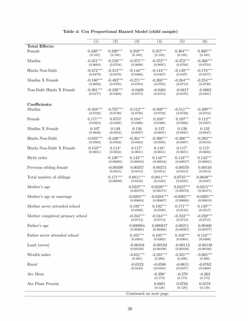
Table 4: Cox Proportional Hazard Model (child sample)

(1) (2) (3) (4) (5) (6)Total Effects:Female 0.430∗∗∗ 0.339∗∗∗ 0.359∗∗∗ 0.357∗∗∗ 0.364∗∗∗ 0.360∗∗∗

(0.105) (0.105) (0.105) (0.105) (0.105) (0.105)

Muslim -0.351∗∗∗ -0.558∗∗∗ -0.375∗∗∗ -0.372∗∗∗ -0.372∗∗∗ -0.366∗∗∗(0.0694) (0.0704) (0.0696) (0.0697) (0.0709) (0.0724)

Hindu Non-Dalit -0.472∗∗∗ -0.312∗∗∗ -0.144∗∗∗ -0.144∗∗∗ -0.149∗∗∗ -0.178∗∗∗(0.0479) (0.0470) (0.0466) (0.0467) (0.0470 (0.0477)

Muslim X Female -0.180∗∗∗ -0.482∗∗∗ -0.271∗∗∗ -0.268∗∗∗ -0.264∗∗∗ -0.254∗∗∗(0.0693) (0.0705) (0.0704) (0.0705) (0.0713) (0.0730)

Non-Dalit Hindu X Female -0.301∗∗∗ -0.236∗∗∗ -0.0409 -0.0401 -0.0417 -0.0662(0.0477) (0.0469) (0.0474) (0.0474) (0.0476) (0.0481)

Coefficients:Muslim -0.458∗∗∗ -0.707∗∗∗ -0.513∗∗∗ -0.509∗∗∗ -0.511∗∗∗ -0.499∗∗∗

(0.0720) (0.0730) (0.0728) (0.0729) (0.0739) (0.0754)

Female 0.171∗∗∗ 0.0757 0.104∗∗ 0.103∗∗ 0.107∗∗ 0.112∗∗(0.0462) (0.0466) (0.0466) (0.0466) (0.0466) (0.0467)

Muslim X Female 0.107 0.149 0.138 0.137 0.139 0.133(0.0946) (0.0952) (0.0947) (0.0947) (0.0947) (0.0947)

Hindu Non-Dalit -0.625∗∗∗ -0.426∗∗∗ -0.261∗∗∗ -0.260∗∗∗ -0.266∗∗∗ -0.293∗∗∗(0.0503) (0.0502) (0.0504) (0.0505) (0.0507) (0.0510)

Hindu Non-Dalit X Female 0.153∗∗ 0.114∗ 0.117∗ 0.116∗ 0.117∗ 0.115∗(0.0651) (0.0652) (0.0651) (0.0651) (0.0651) (0.0650)

Birth order 0.138∗∗∗ 0.143∗∗∗ 0.143∗∗∗ 0.143∗∗∗ 0.143∗∗∗(0.00905) (0.00916) (0.00916) (0.00917) (0.00921)

Previous sibling female -0.00499 0.00357 0.00274 0.00570 0.00510(0.0315) (0.0314) (0.0314) (0.0314) (0.0314)

Total number of siblings 0.171∗∗∗ 0.0811∗∗∗ 0.0811∗∗∗ 0.0735∗∗∗ 0.0649∗∗∗(0.00888) (0.0102) (0.0102) (0.0105) (0.0107)

Mother’s age 0.0227∗∗∗ 0.0228∗∗∗ 0.0227∗∗∗ 0.0215∗∗∗(0.00473) (0.00474) (0.00473) (0.00471)

Mother’s age at marriage -0.0284∗∗∗ -0.0284∗∗∗ -0.0285∗∗∗ -0.0265∗∗∗(0.00604) (0.00607) (0.00608) (0.00619)

Mother never attended school 0.192∗∗∗ 0.192∗∗∗ 0.171∗∗∗ 0.149∗∗∗(0.0509) (0.0509) (0.0510) (0.0517)

Mother completed primary school -0.244∗∗∗ -0.244∗∗∗ -0.243∗∗∗ -0.259∗∗∗(0.0714) (0.0714) (0.0713) (0.0715)

Father’s age 0.000984 0.000917 0.00211 0.00400(0.00365) (0.00366) (0.00367) (0.00377)

Father never attended school 0.105∗∗∗ 0.105∗∗∗ 0.103∗∗∗ 0.116∗∗∗(0.0363) (0.0363) (0.0364) (0.0368)

Land (acres) -0.00104 -0.00103 -0.00113 -0.00148(0.00108) (0.00108) (0.00108) (0.00108)

Wealth index -3.621∗∗∗ -3.591∗∗∗ -3.501∗∗∗ -3.065∗∗∗(0.285) (0.286) (0.290) (0.308)

Rural -0.0523 -0.0508 -0.0615 -0.0762(0.0443) (0.0444) (0.0457) (0.0468)

Ate Meat -0.290∗ -0.279 -0.263(0.173) (0.173) (0.173)

Ate Plant Protein 0.0861 0.0792 0.0578(0.128) (0.129) (0.128)

Continued on next page

26

Table 4: Cox Proportional Hazard Model (child sample)

(1) (2) (3) (4) (5) (6)Ate Dairy 0.0981 0.125 0.118

(0.178) (0.178) (0.177)

Hemelevel -0.00155∗ -0.00152 -0.000893(0.000925) (0.000926) (0.000954)

Average measles vaccinations -0.435∗∗∗ -0.282∗∗(0.110) (0.114)

Average BCG vaccinations 0.0919 0.158(0.157) (0.163)

Average polio vaccinations 0.160 -0.0404(0.127) (0.136)

Average DPT vaccinations 0.0702 0.0599(0.151) (0.156)

Average female LFP -0.00575 0.194∗∗(0.0756) (0.0871)

Average female self-employed 0.0659 0.267(0.151) (0.165)

State Dummies No No No No No YesN 195080 195080 195080 195080 195080 195080Chi-squared 286.7 1977.8 2449.8 2471.8 2502.2 2912.8

Table 4: Cox Proportional Hazard Model. Standard errors in parentheses: ∗ p < 0.10, ∗∗ p < 0.05, ∗∗∗ p < 0.01

27

Tab

le5:

Mor

tali

tyR

egre

ssio

ns

(fem

ale

sam

ple

),D

epen

den

tV

aria

ble

:Fra

ctio

nof

wom

an’s

chil

dre

nw

ho

die

dB

oys

Gir

lsA

llm

oth

ers

Age≥

30A

ge≥

40A

llm

oth

ers

Age≥

30A

ge≥

40(1

)(2

)(3

)(4

)(5

)(6

)(7

)(8

)(9

)(1

0)M

uslim

-0.7

58∗∗

-0.9

86∗∗∗

-1.0

45∗∗∗

-1.4

91∗∗∗

-1.8

98∗∗∗

-0.5

86∗

-0.8

63∗∗∗

-1.0

86∗∗∗

-1.2

86∗∗∗

-1.5

16∗∗∗

(0.3

65)

(0.2

40)

(0.2

27)

(0.2

81)

(0.3

77)

(0.3

38)

(0.2

05)

(0.1

97)

(0.2

64)

(0.3

93)

Hin

duN

on-D

alit

-1.1

66∗∗∗

0.00

612

-0.1

71-0

.201

-0.4

63-0

.916

∗∗∗

0.24

5∗-0

.056

50.

0199

0.06

54(0

.210)

(0.1

58)

(0.1

45)

(0.1

84)

(0.3

05)

(0.2

07)

(0.1

39)

(0.1

00)

(0.1

05)

(0.1

66)

Tot

alC

hild

ren

1.13

0∗∗∗

1.14

5∗∗∗

1.16

3∗∗∗

1.01

9∗∗∗

1.12

0∗∗∗

1.09

8∗∗∗

1.09

4∗∗∗

1.05

5∗∗∗

(0.0

676)

(0.0

622)

(0.0

627)

(0.0

693)

(0.0

703)

(0.0

565)

(0.0

678)

(0.0

699)

Wom

an’s

age

-0.0

204

-0.0

246∗

0.03

08∗

0.04

37-0

.047

3∗∗∗

-0.0

557∗

∗∗-0

.003

070.

0257

(0.0

135)

(0.0

127)

(0.0

169)

(0.0

336)

(0.0

143)

(0.0

131)

(0.0

170)

(0.0

330)

Wom

an’s

age

atm

arri

age

-0.0

237∗

0.00

0853

0.00

0619

0.00

818

-0.0

0182

0.02

28∗

0.02

69∗

0.00

974

(0.0

128)

(0.0

116)

(0.0

130)

(0.0

204)

(0.0

150)

(0.0

117)

(0.0

135)

(0.0

231)

Wom

anne

ver

atte

nded

scho

ol0.

457∗

∗∗0.

391∗

∗∗0.

516∗

∗∗0.

381

0.54

0∗∗∗

0.36

9∗∗∗

0.50

6∗∗∗

0.26

5(0

.126)

(0.1

32)

(0.1

43)

(0.2

68)

(0.1

16)

(0.1

25)

(0.1

49)

(0.3

15)

Wom

anco

mpl

eted

prim

ary

scho

ol-0

.196

-0.1

96∗

0.05

40-0

.190

-0.3

21∗∗

-0.3

23∗∗

-0.1

430.

0183

(0.1

19)

(0.1

13)

(0.1

47)

(0.2

05)

(0.1

31)

(0.1

34)

(0.1

51)

(0.2

12)

Hus

band

’sag

e-0

.015

7-0

.013

1-0

.006

590.

0083

90.

0002

590.

0125

0.01

02-0

.000

0041

7(0

.0110)

(0.0

114)

(0.0

163)

(0.0

236)

(0.0

133)

(0.0

0985)

(0.0

110)

(0.0

194)

Hus

band

neve

rat

tend

edsc

hool

0.17

50.

177

0.14

7-0

.165

0.51

0∗∗∗

0.52

7∗∗∗

0.38

4∗∗

0.45

9∗(0

.125)

(0.1

32)

(0.1

31)

(0.2

49)

(0.1

35)

(0.1

33)

(0.1

63)

(0.2

38)

Lan

d(i

nac

res)

0.00

549∗

∗0.

0041

8∗0.

0032

7-0

.001

310.

0065

0∗∗∗

0.00

451∗

0.00

802∗

∗-0

.004

66(0

.00241)

(0.0

0230)

(0.0

0249)

(0.0

0675)

(0.0

0221)

(0.0

0227)

(0.0

0346)

(0.0

0516)

Wea

lth

inde

x-7

.354

∗∗∗

-5.6

80∗∗∗

-6.3

53∗∗∗

-10.

96∗∗∗

-5.5

85∗∗∗

-4.6

33∗∗∗

-5.3

93∗∗∗

-7.9

30∗∗∗

(0.8

10)

(0.7

28)

(0.8

44)

(1.2

70)

(0.6

24)

(0.6

58)

(0.7

75)

(1.2

56)

Rur

al-0

.177

-0.0

107

-0.0

757

-0.2

07-0

.085

50.

0341

-0.0

685

-0.0

822

(0.1

27)

(0.1

36)

(0.1

57)

(0.2

64)

(0.1

15)

(0.1

15)

(0.1

11)

(0.1

73)

Con

stan

t4.

241∗

∗∗1.

835∗

∗∗1.

007∗

∗-1

.313

∗∗-1

.134

3.59

1∗∗∗

0.99

5∗∗

0.42

2-1

.796

∗∗∗

-1.6

81(0

.368)

(0.3

79)

(0.3

84)

(0.4

77)

(1.3

83)

(0.3

68)

(0.3

88)

(0.3

74)

(0.4

71)

(1.3

63)

Obs

erva

tion

s79

118

7911

879

118

4934

219

518

7911

879

118

7911

849

342

1951

8A

djus

ted

R-s

quar

ed0.

002

0.04

70.

050

0.07

10.

076

0.00

20.

054

0.05

70.

079

0.08

6T

able

5:N

otes

:(i)

Stan

dard

erro

rsin

pare

nthe

ses:

∗p<

0.10

,∗∗p<

0.05

,∗∗∗p<

0.01

.

28

Table 6: Cluster-level mortality regressions (village sample)Fraction of Boys Died Fraction of Girls Died

(1) (2) (3) (4) (5) (6)Muslim population -0.00719 -0.00519 -0.00362 -0.00635 -0.00502 -0.00556∗

(0.00552) (0.00318) (0.00324) (0.00614) (0.00319) (0.00322)

Hindu Non-Dalit population -0.00913∗∗ 0.00144 0.000537 -0.00450 0.00503∗ 0.00114(0.00354) (0.00235) (0.00212) (0.00360) (0.00270) (0.00211)

Average female age 0.000199 0.000172 0.0000599 0.0000116(0.000119) (0.000113) (0.000116) (0.000112)

Average female age at marriage -0.000514∗ -0.000307 -0.000230 0.0000772(0.000279) (0.000261) (0.000237) (0.000259)

Average female education -0.0135∗∗∗ -0.0119∗∗∗ -0.0108∗∗∗ -0.00779∗∗∗(0.00187) (0.00184) (0.00221) (0.00183)

Average male education 0.000496 0.000180 -0.00182 -0.00176(0.00229) (0.00204) (0.00290) (0.00202)

Rural population -0.00170 0.00149 0.00264 0.00575∗∗(0.00248) (0.00233) (0.00295) (0.00231)

Average land (in acres) 0.0000233 0.0000229 0.0000659 0.0000560(0.0000850) (0.0000642) (0.0000641) (0.0000638)

Average wealth index scores -0.0000970∗∗∗ -0.0000811∗∗∗ -0.0000782∗∗∗ -0.0000637∗∗∗(0.0000140) (0.0000134) (0.0000126) (0.0000133)

Average of meat -0.0287 0.0142 -0.0812∗∗∗ -0.00396(0.0176) (0.0206) (0.0149) (0.0205)

Average of plant protein -0.0145 -0.0163 -0.0242 -0.0296∗(0.0152) (0.0179) (0.0189) (0.0178)

Average of dairy -0.0595∗∗ -0.0430∗ -0.0228 0.00292(0.0227) (0.0228) (0.0237) (0.0226)

Average of hemoglobin level -0.000639∗∗∗ -0.000539∗∗∗ -0.000719∗∗∗ -0.000568∗∗∗(0.000164) (0.000147) (0.000164) (0.000146)

Average of measles vaccinations -0.00463 -0.000318 0.000182 0.00416(0.00530) (0.00533) (0.00487) (0.00529)

Average of BCG vaccinations -0.0151 -0.00282 -0.0186 -0.00678(0.0115) (0.00952) (0.0115) (0.00946)

Average of polio vaccinations 0.0322∗∗ 0.0200∗∗ 0.0370∗∗∗ 0.0116(0.0126) (0.00827) (0.0128) (0.00822)

Average of DPT vaccinations -0.0159∗ -0.0127 -0.0287∗∗∗ -0.0186∗∗(0.00835) (0.00949) (0.00935) (0.00943)

Average female LFP 0.000960 0.00657 -0.00298 0.00778(0.00654) (0.00476) (0.00607) (0.00473)

Average female self-employment 0.00112 -0.00559 0.0162 0.0114(0.0112) (0.00943) (0.0118) (0.00938)

Constant 0.0766∗∗∗ 0.185∗∗∗ 0.158∗∗∗ 0.0656∗∗∗ 0.189∗∗∗ 0.155∗∗∗(0.00546) (0.0195) (0.0187) (0.00572) (0.0208) (0.0186)

State Fixed Effects No No Yes No No YesN 3644 3637 3637 3644 3637 3637R-squared 0.00487 0.202 0.236 0.00152 0.201 0.250

Table 6: Regressions based on 3644 clusters. Standard errors in parentheses: ∗ p < 0.10, ∗∗ p < 0.05, ∗∗∗ p < 0.01.

29