mipr lecture 7 copyright oleh tretiak, 2004 1 medical imaging and pattern recognition lecture 7...

MIPR Lecture 7Copyright Oleh Tretiak, 2004

1

Medical Imaging and Pattern Recognition

Lecture 7 Computed Tomography

Oleh Tretiak


2

Computer Tomography:How It Works

Only one plane is illuminated. Source-subject motion provides added information.


3

How it Works

• Original CT Scanner– Head only– One minute scanning time– Two sections– Ten minutes to compute images– Extremely successful!


4

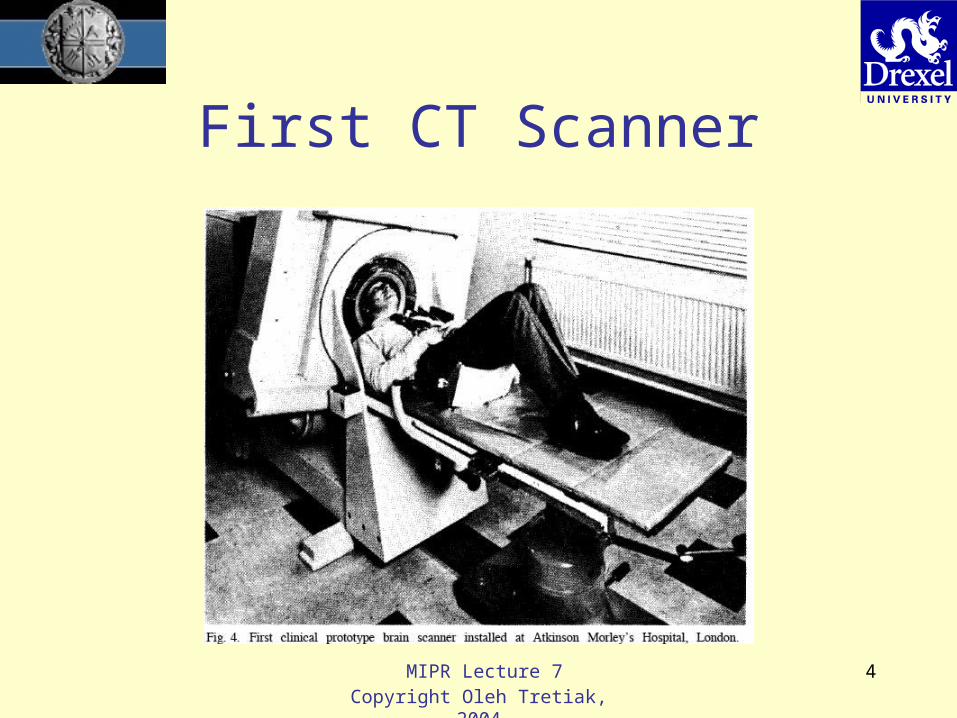
First CT Scanner


5

Before and After CT


6

Contemporary CT


7

Fan-Beam Computer Tomography


8

Contemporary Spiral Scanner

• Configuration:– 40 slices per rotation maximum

• Other options are 32 slices or 16 slices

– 40 mm axial distance scanned in one rotation

– 0.4 sec per rotation– 60 kW generator


9

Example: Head

• Bleeding due to injury

• Can cause brain injury if not treated

• Blood between brain and dura, easy to treat


10

Example: Head

• FRONTAL CONTUSION WITH SUBARACHNOID HEMORRHAGE


11

Chest Study

• Pneumothorax (air between lung and chest)

• Also note the bilateral lower lobe consolidation of lungs, right being greater than left. There is a chest tube within the right hemithorax.


12

Abdomen

• Appendicitis (arrow)

• Contrast agents in stomach and in blood


13

Mathematics of Computed Tomography

• Model for measurements• Direct problem• Inverse problem• Algorithm for computed

tomography


14

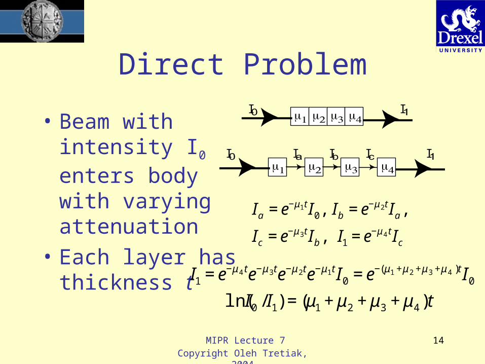
Direct Problem

• Beam with intensity I0 enters body with varying attenuation

• Each layer has thickness t

m m m mI I

m m m mI II I I

€

€

Ia = e−μ1tI0, Ib = e−μ 2tIa ,

Ic = e−μ 3tIb , I1 = e−μ 4 tIc

€

I1 = e−μ 4 te−μ 3te−μ 2te−μ1tI0 = e−(μ1 +μ 2 +μ 3 +μ 4 )tI0ln(I0 /I1) = (μ1 + μ2 + μ3 + μ4 )t


15

Integral Equation

x

I (y)I

€

I1(y) = exp(− μ(x,y)dx∫ )I0

ln(I0 /I1(y)) = μ(x,y)dx∫

x

I (t, q)

I

y

q

t

€

ln(I0 /I1(t,θ)) = μ(t cosθ − lsinθ, t sinθ + lcosθ)dl∫


16

Radon Transform

x

I (t, q)

I

y

q

t

f(x,y)

g(t, )

€

g(t,θ) = f (t cosθ − lsinθ, t sinθ + lcosθ)dl∫


17

Inverse Radon Transform

• Given: X-ray transmission measurements I1(t, ). Find (x, y)

• Given: g(t, ). Find f(x, y)• Method:

– (a) convolution

– (b) backprojection

€

f (x,y) = g1(x cosθ + y sinθ,θ)dθ0

π

∫€

g1(t,θ) = h(t − τ )g(τ ,θ)dτ∫


18

Example

-1

0

1

-1

0

1

-0.5

0

0.5

1

-1 -0.5 0 0.5 1

-0.6

-0.4

-0.2

0

0.2

0.4

0.6

0.8

1

1.2

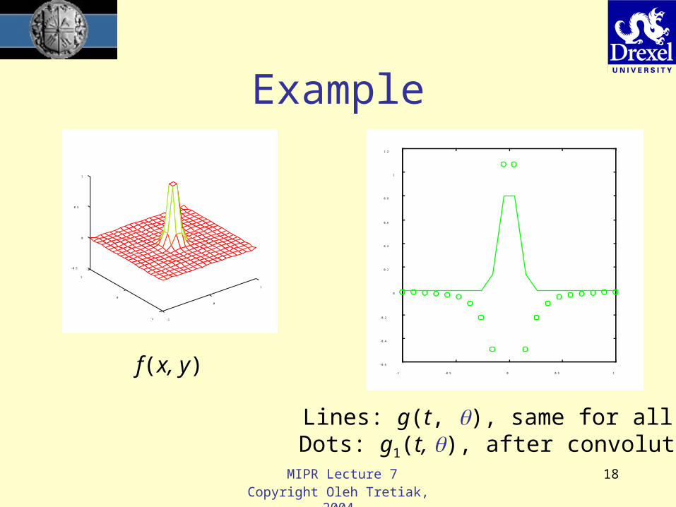
f(x, y)

Lines: g(t, ), same for all Dots: g1(t, ), after convolution


19

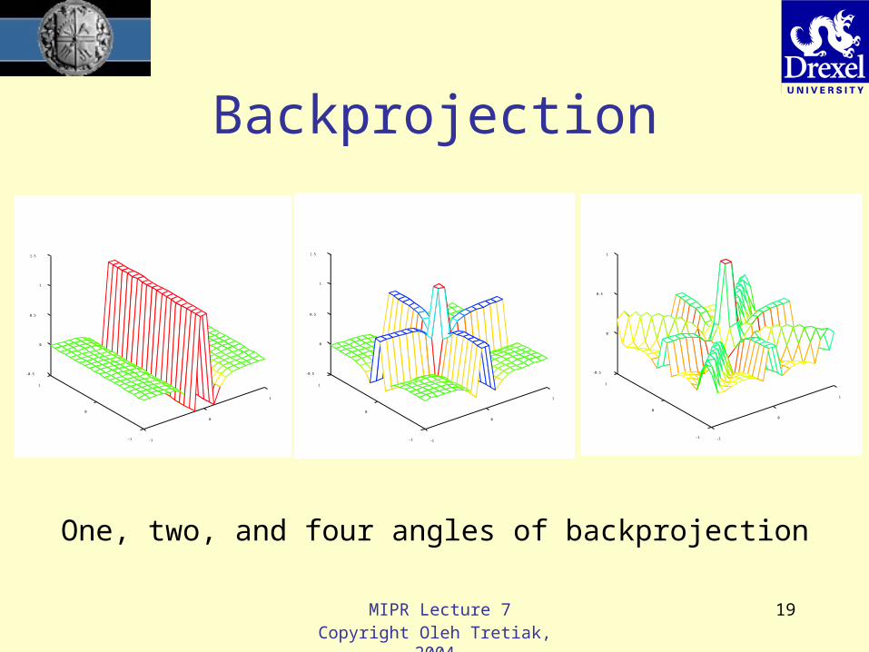
Backprojection

-1

0

1

-1

0

1

-0.5

0

0.5

1

1.5

One, two, and four angles of backprojection

-1

0

1

-1

0

1

-0.5

0

0.5

1

1.5

-1

0

1

-1

0

1

-0.5

0

0.5

1


20

More Backprojection

-1

0

1

-1

0

1

-0.5

0

0.5

1

-1

0

1

-1

0

1

-0.5

0

0.5

1

-1

0

1

-1

0

1

-0.5

0

0.5

1

8, 15, and 30 angle backprojection


21

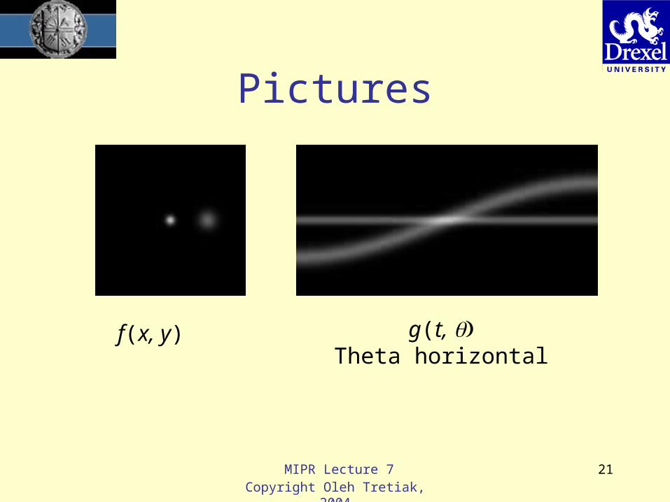
Pictures

f(x, y) g(t, Theta horizontal


22

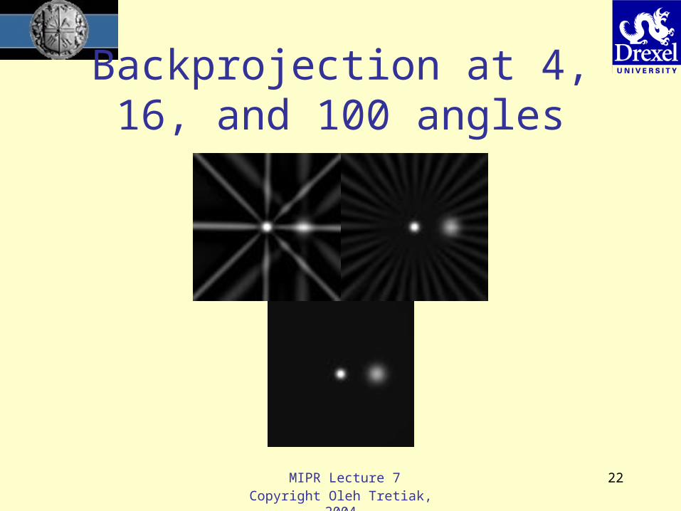
Backprojection at 4, 16, and 100 angles


23

History

• 1917, Joachim Radon– Solved formal inverse problem.

Interest in theory of integration and geometry

• 1958, Simeon Tetelbaum of KPI publishes a paper about X-ray tomography. – Publishes valid inverse problem

solution.


24

More History

• 1963 John Cormack publishes theoretical and experimental results.– Experiment with cylindrical objects

• 1972 Godfrey Hounsfield develops CT scanner

• 1979 Hounsfield and Cormack receive Nobel prize in Medicine


25

Example of Contrast

QuickTime™ and aTIFF (Uncompressed) decompressor

are needed to see this picture.

12 bit image, full contrast range.

Window for lowdensities


26

More Contrast Operations

QuickTime™ and aTIFF (Uncompressed) decompressor

are needed to see this picture.

Window for highdensities


27

3-D Images

• Spiral scan procedures produce sets of sectional images suitable for 3-D imaging

• Resectioning: Compute new section plane

• Projection: Compute sums along rays• Rendering: Segment image and show

surface.


28

Bronchoscopy

Path View


29

Colonoscopy

Path View


30

Medical Practice

• In the fall of 2003 Siemens became the first CT supplier ever to receive clearance from the FDA for a computer-aided technique of identifying nodules, that is, possible tumors, in the lung. CT is also used for the diagnosis of colon cancer: A virtual flight through the human colon can detect even the smallest polyps. If these are removed in time, an outbreak of colon cancer can very probably be prevented.


31

Comparison

Left: A polyp seen with optical endoscopy. Right: View in virtual endoscopy.


32

Summary

• Computer tomography became successful because it showed soft tissue differences that could not be seen on X-rays.

• Evolution of high-speed (spiral scan) machines came about through improvements in X-ray detectors

• This has led to 3-D imaging methods– Surgery planning– Virtual endoscopy

mipr lecture 7 copyright oleh tretiak, 2004 1 medical imaging and pattern recognition lecture 7...

Documents