Minitab 14

1

GETTING STARTED

To OPEN MINITAB: Click Start>Programs>Minitab14>Minitab14 orClick Minitab 14 on your Desktop

The Minitab session will come up like this

2

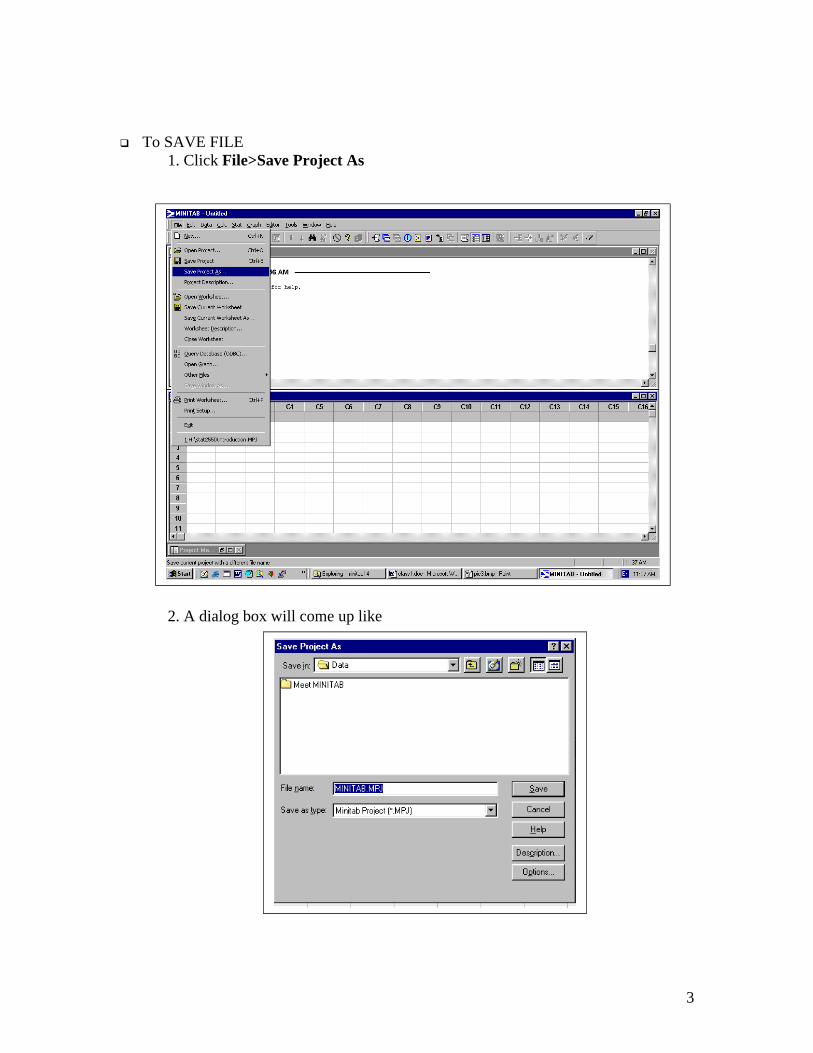
To SAVE FILE1. Click File>Save Project As

2. A dialog box will come up like

3

3. Do the followings

To OPEN A SAVED FILE1. click File>Open Project

4

Click to make new folder

Type the folder nameand press enter

Type the file name andpress enter

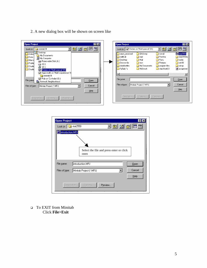
2. A new dialog box will be shown on screen like

To EXIT from MinitabClick File>Exit

5

Select the file and press enter or clickopen

Using CALCULATOR

Sometimes we need to manipulate variables. For example, suppose we are given Height(in inch) of 10 students, but we want it in Feet.

Height: 65, 66, 64, 68, 65, 67, 66, 70, 72, 68

That is, we want to convert the variable and get a new one with units in feet. The rules forconverting variable is very simple

Converting Variable

1. Go to ‘Calculation’ from Menu-bar2. Click ‘Calculator’3. Write the variable name in ‘Store result in variable’.

(you can use the same variable name, then the earlier variable will be replaced bythe converted one or you can use different variable name)

4. Then in the ‘Expression’, mention what to calculate.

Calculation of Height (inch) into Height (ft)

1. Go to ‘Calculation’ from Menu-bar2. Click ‘Calculator’3. Write the variable name in ‘Height Ft’.

(If you use ‘Height’, then the values of Height will be replaced by new one, i.e. 1st

value of Height 65 will be replaced by 5.41667 and so on)4. Then in the ‘Expression’, write ‘Height’ / 12

(There are many other options functions located in the ‘Function’ scroll menu).

Question:

The table below is the scores of 50 students in a mathematics course:

62509371555119725847

48629954585657566143

77507983625568716564

90857522557549616377

76586179705960634158

Construct a stem-and-leaf display for all 50 scoresConstruct a histogram for all 50 scoresCalculate the mean, median and variance of all scores

6

Inputting Data In Minitab:

1. Input data in Worksheet Window.2. Input variables in columns.3. First row of worksheet window can be used for variables names.

Minitab Project Report

(a)

Steps: 1. Go to the menu "Graph"2. Select: "Stem-and-leaf"3. Select the variable "Score"4. Write the increment = 105. Click "OK"

7

Output:

Stem-and-leaf of Score N = 50Leaf Unit = 1.0

1 1 9 2 2 2 2 3 7 4 13789 22 5 001455566788889 (12) 6 011122233458 16 7 01125567799 5 8 35 3 9 039

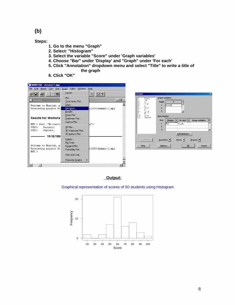
(b)

Steps: 1. Go to the menu "Graph"2. Select: "Histogram"3. Select the variable "Score" under 'Graph variables'4. Choose "Bar" under 'Display' and "Graph" under 'For each'5. Click "Annotation" dropdown menu and select "Title" to write a title of the graph6. Click "OK"

Output:

20 30 40 50 60 70 80 90 100

0

10

20

Score

Freq

uenc

y

Graphical representation of scores of 50 students using Histogram

8

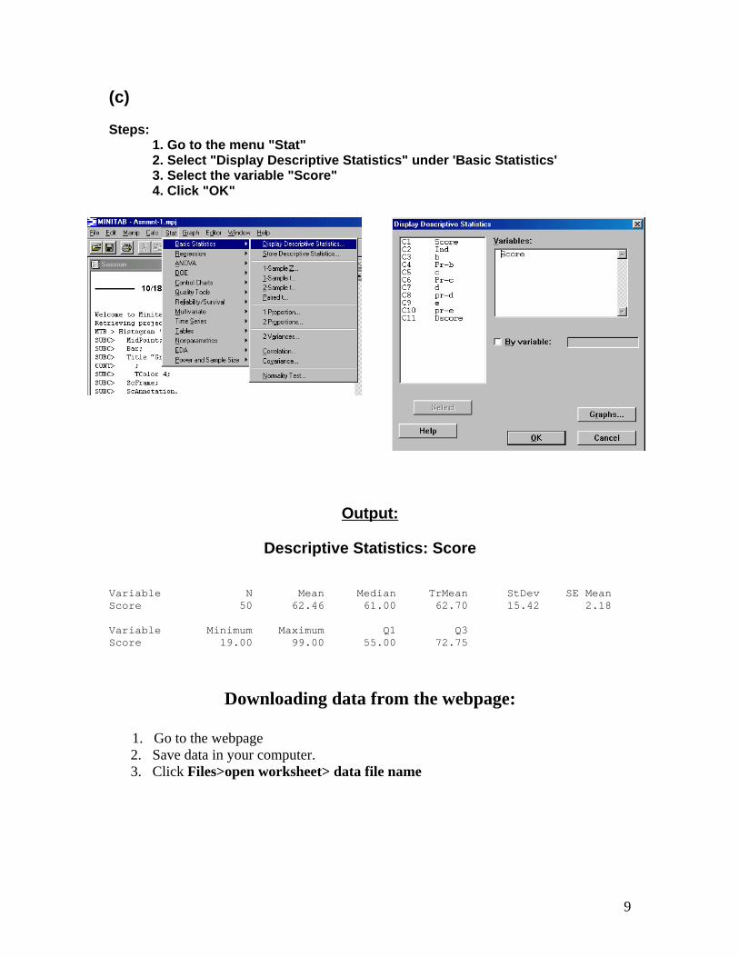
(c)

Steps: 1. Go to the menu "Stat"2. Select "Display Descriptive Statistics" under 'Basic Statistics'3. Select the variable "Score"4. Click "OK"

Output:

Descriptive Statistics: Score

Variable N Mean Median TrMean StDev SE MeanScore 50 62.46 61.00 62.70 15.42 2.18

Variable Minimum Maximum Q1 Q3Score 19.00 99.00 55.00 72.75

Downloading data from the webpage:

1. Go to the webpage2. Save data in your computer.3. Click Files>open worksheet> data file name

9

FINDING PROBABILITIES (BINOMIAL DISTRIBUTION)

Suppose x is a binomial random variable. Use MINITAB to find the followingprobabilities:

(a) P(x = 4) for n = 10, p = 0.3 (b) P(x >= 6) for n = 10, p = 0.3(c) P(1 < x < 9) for n = 15, p = 0.4(d) P(x > 5) for n = 15, p = 0.4(e) P(x<4) for n=15, p=0.4(f) For n = 10, p = 0.3, obtain the plot of the binomial distribution.

Steps: 1. Go to Menu "Calc" > "Probability distribution" > "Binomial"2. Select: Probability, No. of trials, Probability of success and "Input constant"

1. Click "OK"

Solution

Figure: Calculation of 3 (a)

Find P(x=4) for n=10, p=0.3P(X = 3) = 0.2668

b) Find P(x>=6) for n=10, p=0.3 P(X >= 6) = P(X = 6) + ... + P(X = 10) = 1- P(X = 0) + P(X = 1)

+ ... + P(X = 5)= 1- (0.028248 + 0.121061+ 0.233474 + 0.266828

10

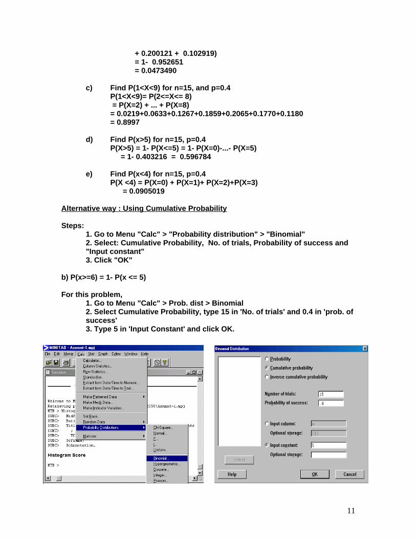
+ 0.200121 + 0.102919)= 1- 0.952651= 0.0473490

c) Find P(1<X<9) for n=15, and p=0.4P(1<X<9)= P(2<=X<= 8) = P(X=2) + ... + P(X=8)= 0.0219+0.0633+0.1267+0.1859+0.2065+0.1770+0.1180= 0.8997

d) Find P(x>5) for n=15, p=0.4P(X>5) = 1- P(X<=5) = 1- P(X=0)-...- P(X=5) = 1- 0.403216 = 0.596784

e) Find P(x<4) for n=15, p=0.4P(X <4) = P(X=0) + P(X=1)+ P(X=2)+P(X=3) = 0.0905019

Alternative way : Using Cumulative Probability

Steps: 1. Go to Menu "Calc" > "Probability distribution" > "Binomial"2. Select: Cumulative Probability, No. of trials, Probability of success and "Input constant"3. Click "OK"

b) P(x>=6) = 1- P(x <= 5)

For this problem, 1. Go to Menu "Calc" > Prob. dist > Binomial2. Select Cumulative Probability, type 15 in 'No. of trials' and 0.4 in 'prob. ofsuccess'3. Type 5 in 'Input Constant' and click OK.

Output

11

Cumulative Distribution Function

Binomial with n = 10 and p = 0.3

x P( X <= x )5 0.952651

Thus, P(x >= 6 ) = 1- 0.952651 = 0.0473490

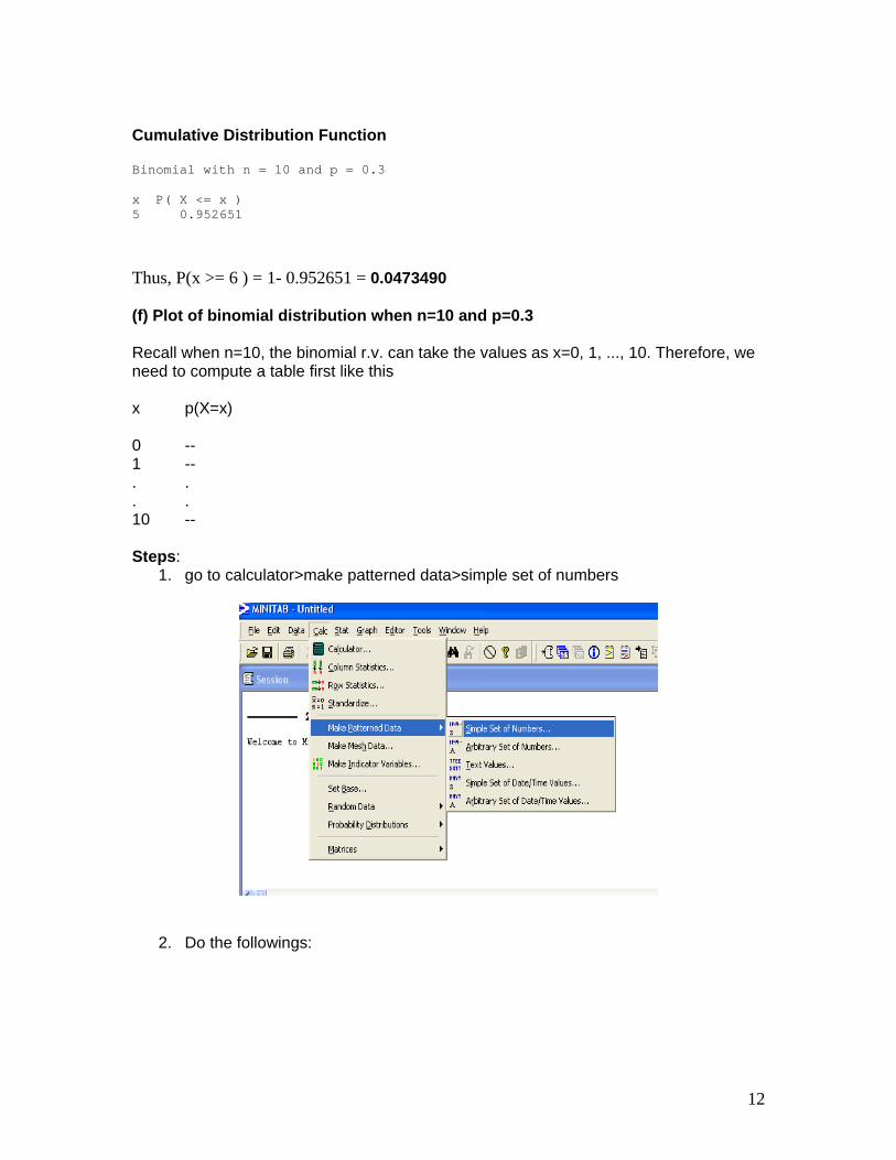
(f) Plot of binomial distribution when n=10 and p=0.3

Recall when n=10, the binomial r.v. can take the values as x=0, 1, ..., 10. Therefore, weneed to compute a table first like this

x p(X=x)

0 --1 --. .. .10 --

Steps:1. go to calculator>make patterned data>simple set of numbers

2. Do the followings:

12

3.

13

then go to graph> bar chart and do this

The binomial graph is then have the shape:

14

C1

C2

109876543210

0.30

0.25

0.20

0.15

0.10

0.05

0.00

Chart of C2 vs C1

Finding Probabilities for Normal Distribution

Steps: • Go to ‘Calc’ → ‘Probability Dist’ → ‘Normal’• Select ‘Cumulative probability’, ‘Mean’ ‘St. Deviation’ • Select input constant• If you type 0.3 in ‘Input Constant’, you will have the probability that X lies

between (- ∞, 0.3)

Output

Cumulative Distribution Function

Normal with mean = 0 and standard deviation = 1.00000

x P( X <= x ) 0.3000 0.6179

Problem 1: The random variable X has a normal distribution with μ=70 and σ=10. Findthe following probabilities:

a) P(X<75) b) P(X ≥ 90) c) P(60 ≤ X ≤ 75)

15

Figure: Calculation of P(x ≤ 0.3), when Mean = 0 and Variance = 1

Problem 2: Assume that X is a binomial random variable with n=100 and p=0.5.Calculate the exact binomial probability and the approximation obtained by using thenormal distribution for a) P(X ≤ 48) b) P(50 ≤ X ≤ 65) c) P(X ≥ 70)

Hints: For normal approximation:

• P(X ≤ 48) = P(X ≤ 48.5)(approx)

• P(50 ≤ X ≤ 65)= P(X ≤ 65) – P(X ≤ 49) = P(X ≤ 65.5)–P(X ≤ 49.5) (approx)

• P(X ≥ 70) = 1-P(X<70) = 1-P(X ≤ 69) = 1- P(X ≤ 69.5) (approx)

Then obtain those probabilities from normal distribution using μ = np, σ = npq.

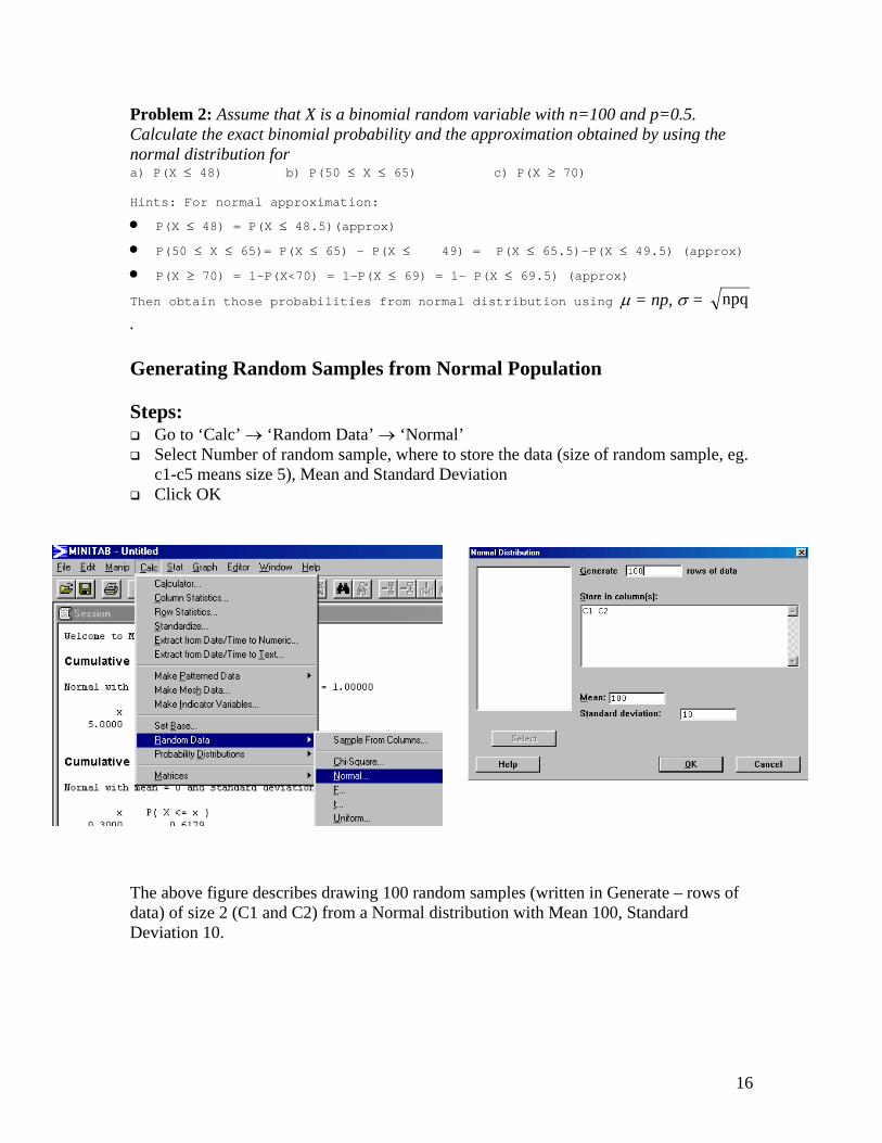
Generating Random Samples from Normal Population

Steps: Go to ‘Calc’ → ‘Random Data’ → ‘Normal’Select Number of random sample, where to store the data (size of random sample, eg.c1-c5 means size 5), Mean and Standard DeviationClick OK

The above figure describes drawing 100 random samples (written in Generate – rows ofdata) of size 2 (C1 and C2) from a Normal distribution with Mean 100, StandardDeviation 10.

16

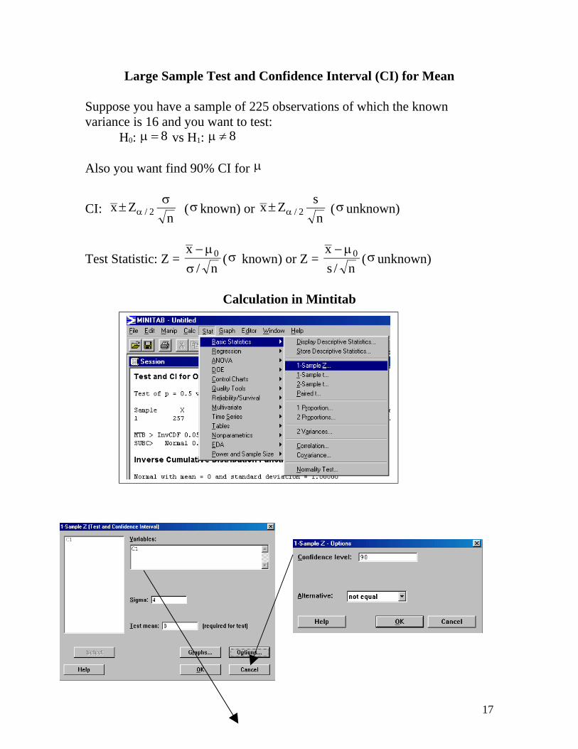
Large Sample Test and Confidence Interval (CI) for Mean

Suppose you have a sample of 225 observations of which the knownvariance is 16 and you want to test:

H0: 8=μ vs H1: 8≠μ

Also you want find 90% CI for μ

CI: n

Zx 2/σ

± α (σknown) or nsZx 2/α± (σunknown)

Test Statistic: Z = n/

x 0

σμ−

(σ known) or Z = n/s

x 0μ− (σunknown)

Calculation in Mintitab

17

OUTPUTTest of mu = 8 vs mu not = 8The assumed sigma = 4

Variable N Mean StDev SE MeanC1 225 11.565 4.010 0.267Variable 90.0% CI Z PC1 ( 11.127, 12.004) 13.37 0.000

Large Sample Test and Confidence Interval for Proportion

Confidence IntervalExample: 7.4 (Page: 310, Ninth Edition)

Confidence Interval nq̂p̂Zp̂ 05.0±

n = Number of trials: 484, x = number of successes: 257

Calculation in Mintitab

18

The data is located in 1st Column (C1)

Small Sample (n<30) Test and Confidence Interval (CI) for Mean

Formula:

100(1-α)% CI for mean

CI: ⎟⎠

⎞⎜⎝

⎛± α n

stx 2/ where 2/tα is based on (n-1) degrees of freedom (df).

Test Statistic:

For testing, H0: 0μ=μ vs H1: 0μ≠μ

t = n/s

x 0μ− , where t has student’s t-distribution with (n-1) df.

Example

Given a sample14, 9, 12, 14, 10, 9, 10, 12, 11, 9, 6, 2, 14, 10, 11, 12, 9, 6, 4, 8

Test a) 10:H0 =μ vs 10:H1 ≠μb) 10:H0 =μ vs 10:H1 >μc) 10:H0 =μ vs 10:H1 <μ

at 5% level of significance, 10% level of significance

Find 95% confidence interval for μ

Solution:Note that, here the sample size n = 20 (<30), i.e. we have a small sample and alsopopulation standard deviation σ is unknown. So we have to use t-distribution to performthe test and to find the confidence interval after estimating σ by the sample standarddeviation S.

19

Calculation in Mintitab

OUTPUTOne-Sample T:

Test of mu = 10 vs not = 10

Variable N Mean StDev SE Mean 95% CI T Pex-2 20 9.65000 3.21632 0.71919 (8.14471, 11.15529) -0.49 0.632

In the output T (= -0.49) is the value of the corresponding test statistics and ‘P’ is the p-valuewhich is 0.632.

If the p-value is less than or equal to your level (α ), you can reject H0 .

20

Proportion Test for large sample

Test H0 : p = 0.5 vs H1: p < 0.5

Test Statistic: Z =

nqppp̂

00

0−, 300/10p̂ = , 5.0p0 = , q0 = 1-p0, n = 300

α = 0.01 (1%)Using Minitab

OUTPUT:

Test of p = 0.05 vs p < 0.05

Sample X N Sample p 99.0% Upper Bound Z-Value P-Value1 10 300 0.033333 0.057443 -1.32 0.093

Acknowledgments: This work was mostly done by Taslim S. mallick, Dept. ofMathematics & Statistics, Memorial University of Newfoundland.

21