minitab 14 manual - ksu facultyfac.ksu.edu.sa/sites/default/files/mt14_manual_1.pdf · minitab 14...
TRANSCRIPT

MINITAB 14 Supplement for: Biostatistics for
the Health Sciences
R. Clifford Blair
and
Richard A. Taylor
December 30, 2007

2
c© R. Clifford Blair and Richard A. Taylor 2005
All rights reserved. No part of this publication may be reproduced, storedin a retrieval system, or transmitted, in any form or by any means, electronic,mechanical, photocopying, recording, or otherwise, without the prior permissionof R. Clifford Blair or Richard A. Taylor.
i
Preface
This manual is not an introduction to MININITAB r© and contains only a por-tion of the material that would be contained therein.1 Rather, this manualteaches the reader how to use MINITAB Release 14 for Windows to analyzedata related to the problems addressed in Biostatistics For The Health Sciencesby R. Clifford Blair and Richard A. Taylor.
To this end, MINITAB is used to analyze various of the data sets and prob-lems contained in that text. The reader will be required, especially in the earlypart of the manual, to input selected data to the system. Additional data setsaccompany this manual so that the reader will not be burdened with data entryonce this skill is acquired.
It is assumed that the reader is familiar with the Microsoft Windows r© op-erating system so that little instruction in this regard will be provided. It isfurther assumed that the reader is using MINITAB Release 14 rather than someearlier version.
Chapter 1 familiarizes the reader with some basic MINITAB concepts. Keyamong these is the entry and saving of data which is prerequisite to all thatfollows. Chapters 2 through 10 address the corresponding chapters in the text.That is, Chapter 2 in the manual addresses problems in Chapter 2 in the textand so on. Section headings in these latter chapters reflect the sections/pages inthe text addressed in that section of the manual. Thus, while studying the textreaders can quickly locate the comparable area in the manual by referring tothe manual’s table of contents. In addition, a manual appendix relates specificexamples, data tables etc. in the text to specific pages in the manual. Theseprovisions allow easy integration of MINITAB analyses as study of the textprogresses.
Finally, we would caution that data analysis, whether by hand calculationsor software is no substitute for a clear understanding of the underlying statisticalconcept. Such analysis can, however, be an invaluable aid to mastery of suchconcepts and is indispensable for research purposes.
1The definitive introduction to the MINITABr©
analysis system is found in MINITABr©
Handbook by Barbara Ryan, Brian Joiner, and Jonathon Cryer published by Thomson.

ii

Contents
1 Preliminaries 11.1 Introduction . . . . . . . . . . . . . . . . . . . . . . . . . . . . . . 11.2 Getting Started . . . . . . . . . . . . . . . . . . . . . . . . . . . . 11.3 Inputting Data . . . . . . . . . . . . . . . . . . . . . . . . . . . . 21.4 Performing Analyses . . . . . . . . . . . . . . . . . . . . . . . . . 41.5 Editing and Printing Your Output . . . . . . . . . . . . . . . . . 61.6 Using the Calculator . . . . . . . . . . . . . . . . . . . . . . . . . 61.7 Graphs . . . . . . . . . . . . . . . . . . . . . . . . . . . . . . . . . 8Exercises . . . . . . . . . . . . . . . . . . . . . . . . . . . . . . . . . . 10
2 Descriptive Methods 112.1 Introduction . . . . . . . . . . . . . . . . . . . . . . . . . . . . . . 112.4 Distributions . . . . . . . . . . . . . . . . . . . . . . . . . . . . . 112.5 Graphs . . . . . . . . . . . . . . . . . . . . . . . . . . . . . . . . . 152.6 Numerical Methods . . . . . . . . . . . . . . . . . . . . . . . . . . 24Exercises . . . . . . . . . . . . . . . . . . . . . . . . . . . . . . . . . . 30
3 Probability 313.1 Introduction . . . . . . . . . . . . . . . . . . . . . . . . . . . . . . 313.3 Contingency Tables . . . . . . . . . . . . . . . . . . . . . . . . . . 313.4 The Normal Curve . . . . . . . . . . . . . . . . . . . . . . . . . . 31Exercises . . . . . . . . . . . . . . . . . . . . . . . . . . . . . . . . . . 33
4 Introduction to Inference and One Sample Methods 354.1 Introduction . . . . . . . . . . . . . . . . . . . . . . . . . . . . . . 354.2 Sampling Distributions . . . . . . . . . . . . . . . . . . . . . . . . 354.3 Hypothesis Testing . . . . . . . . . . . . . . . . . . . . . . . . . . 364.4 Confidence Intervals . . . . . . . . . . . . . . . . . . . . . . . . . 42Exercises . . . . . . . . . . . . . . . . . . . . . . . . . . . . . . . . . . 44
5 Paired Samples Methods 455.1 Introduction . . . . . . . . . . . . . . . . . . . . . . . . . . . . . . 455.2 Methods Related to Mean Difference . . . . . . . . . . . . . . . . 455.3 Methods Related to Proportions . . . . . . . . . . . . . . . . . . 46
iii

iv CONTENTS
5.4 Methods Related to Paired Samples Risk Ratios . . . . . . . . . 485.5 Methods Related to Paired Samples Odds Ratios . . . . . . . . . 49Exercises . . . . . . . . . . . . . . . . . . . . . . . . . . . . . . . . . . 52
6 Two Independent Samples Methods 536.1 Introduction . . . . . . . . . . . . . . . . . . . . . . . . . . . . . . 536.2 Methods Related to Differences Between Means . . . . . . . . . . 536.3 Methods Related to Proportions . . . . . . . . . . . . . . . . . . 556.4 Methods Related to Independent Samples Risk Ratios . . . . . . 566.5 Independent Samples Odds Ratios . . . . . . . . . . . . . . . . . 56Exercises . . . . . . . . . . . . . . . . . . . . . . . . . . . . . . . . . . 57
7 Multi-Sample Methods 597.1 Introduction . . . . . . . . . . . . . . . . . . . . . . . . . . . . . . 597.2 The One-Way Analysis of Variance (ANOVA) F Test . . . . . . . 597.3 The 2 By k Chi-Square Test . . . . . . . . . . . . . . . . . . . . . 607.4 Multiple Comparison Procedures . . . . . . . . . . . . . . . . . . 61Exercises . . . . . . . . . . . . . . . . . . . . . . . . . . . . . . . . . . 63
8 The Assessment of Relationships 658.1 Introduction . . . . . . . . . . . . . . . . . . . . . . . . . . . . . . 658.2 The Pearson Product-Moment Correlation Coefficient . . . . . . 658.3 The Chi-Square Test for Independence . . . . . . . . . . . . . . . 66Exercises . . . . . . . . . . . . . . . . . . . . . . . . . . . . . . . . . . 67
9 Linear Regression 699.1 Introduction . . . . . . . . . . . . . . . . . . . . . . . . . . . . . . 699.2 Simple Linear Regression . . . . . . . . . . . . . . . . . . . . . . 699.3 Multiple Linear Regression . . . . . . . . . . . . . . . . . . . . . 70Exercises . . . . . . . . . . . . . . . . . . . . . . . . . . . . . . . . . . 73
10 Methods Based on the Permutation Principle 7510.1 Introduction . . . . . . . . . . . . . . . . . . . . . . . . . . . . . . 7510.3 Applications . . . . . . . . . . . . . . . . . . . . . . . . . . . . . . 75Exercises . . . . . . . . . . . . . . . . . . . . . . . . . . . . . . . . . . 78
A Table Relating Text Items to Tasks 79
Chapter 1
Preliminaries
1.1 Introduction
The hand calculations you perform in conjunction with your studies of thestatistical concepts in Biostatistics For The Health Sciences by R. Clifford Blairand Richard A. Taylor1 are designed to enhance your understanding of theconcepts under study. Modern statistical practice only rarely resorts to suchmethods for the analysis of data collected for research purposes. This is because(1) data sets collected in applied research contexts are often too large for handcalculations and (2) such calculations are prone to errors. Instead, researchersresort to tried and true statistical software that can be relied upon to providequick, accurate results. The MINITAB system is one of the most popular ofthese.
In this manual, you will learn to use MINITAB to analyze data associatedwith the problems outlined in the text. You will learn some basic MINITABconcepts in this chapter. Chapters 2 through 10 will address problems in thelike numbered chapters in the text.
1.2 Getting Started
Before starting MINITAB, you should make yourself a directory in which tostore your work. I’ve called my directory bhs dir. You should then copy thefiles that accompany this manual into your directory.
To start MINITAB you can either double click the MINITAB shortcut icon
on the desktop or select the sequence Start⇒Programs⇒MINITAB 14.The notation Start⇒Programs⇒MINITAB 14 means that you are to firstselect the Start menu, then Programs, and finally MINITAB 14. We will usethis notation throughout this manual.
1Henceforth referred to as “the text”.
1
2 CHAPTER 1. PRELIMINARIES
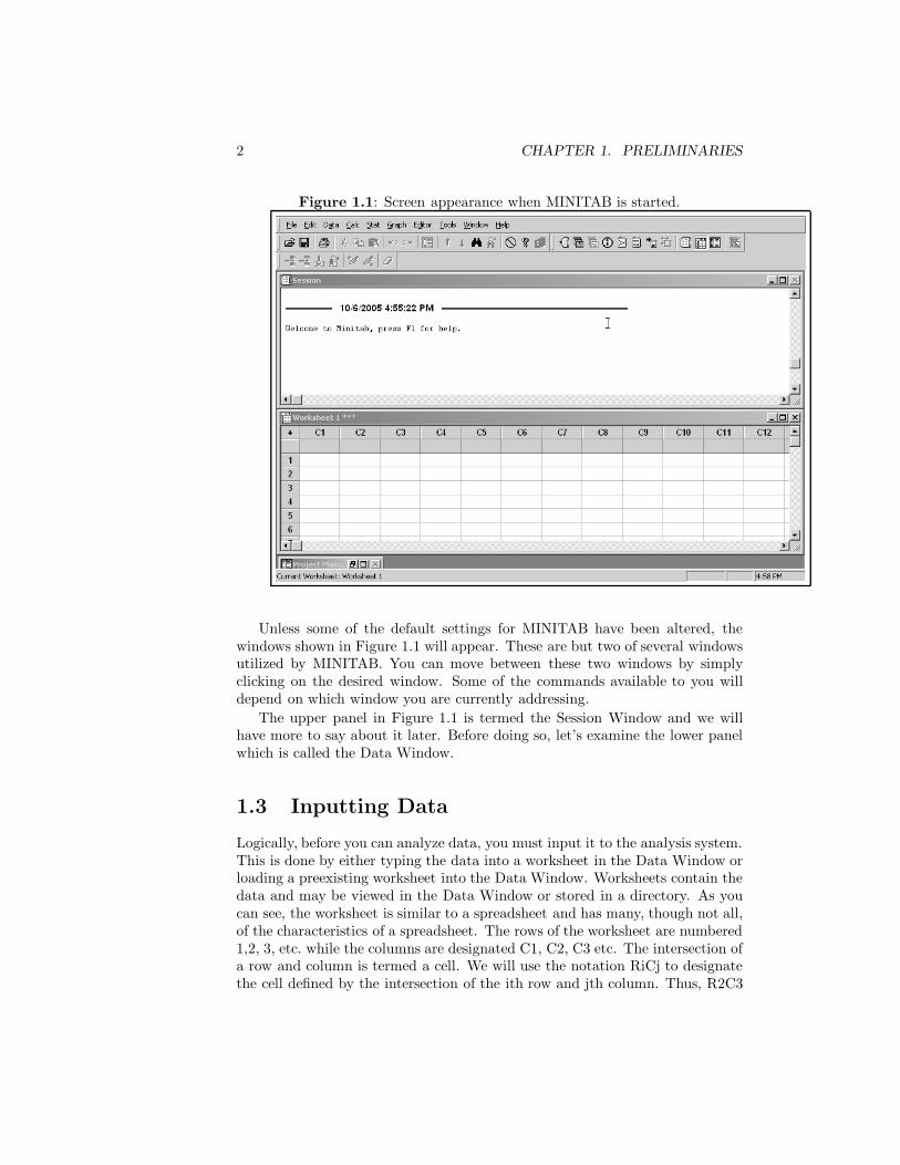
Figure 1.1: Screen appearance when MINITAB is started.
Unless some of the default settings for MINITAB have been altered, thewindows shown in Figure 1.1 will appear. These are but two of several windowsutilized by MINITAB. You can move between these two windows by simplyclicking on the desired window. Some of the commands available to you willdepend on which window you are currently addressing.
The upper panel in Figure 1.1 is termed the Session Window and we willhave more to say about it later. Before doing so, let’s examine the lower panelwhich is called the Data Window.
1.3 Inputting Data
Logically, before you can analyze data, you must input it to the analysis system.This is done by either typing the data into a worksheet in the Data Window orloading a preexisting worksheet into the Data Window. Worksheets contain thedata and may be viewed in the Data Window or stored in a directory. As youcan see, the worksheet is similar to a spreadsheet and has many, though not all,of the characteristics of a spreadsheet. The rows of the worksheet are numbered1,2, 3, etc. while the columns are designated C1, C2, C3 etc. The intersection ofa row and column is termed a cell. We will use the notation RiCj to designatethe cell defined by the intersection of the ith row and jth column. Thus, R2C3
1.3. INPUTTING DATA 3
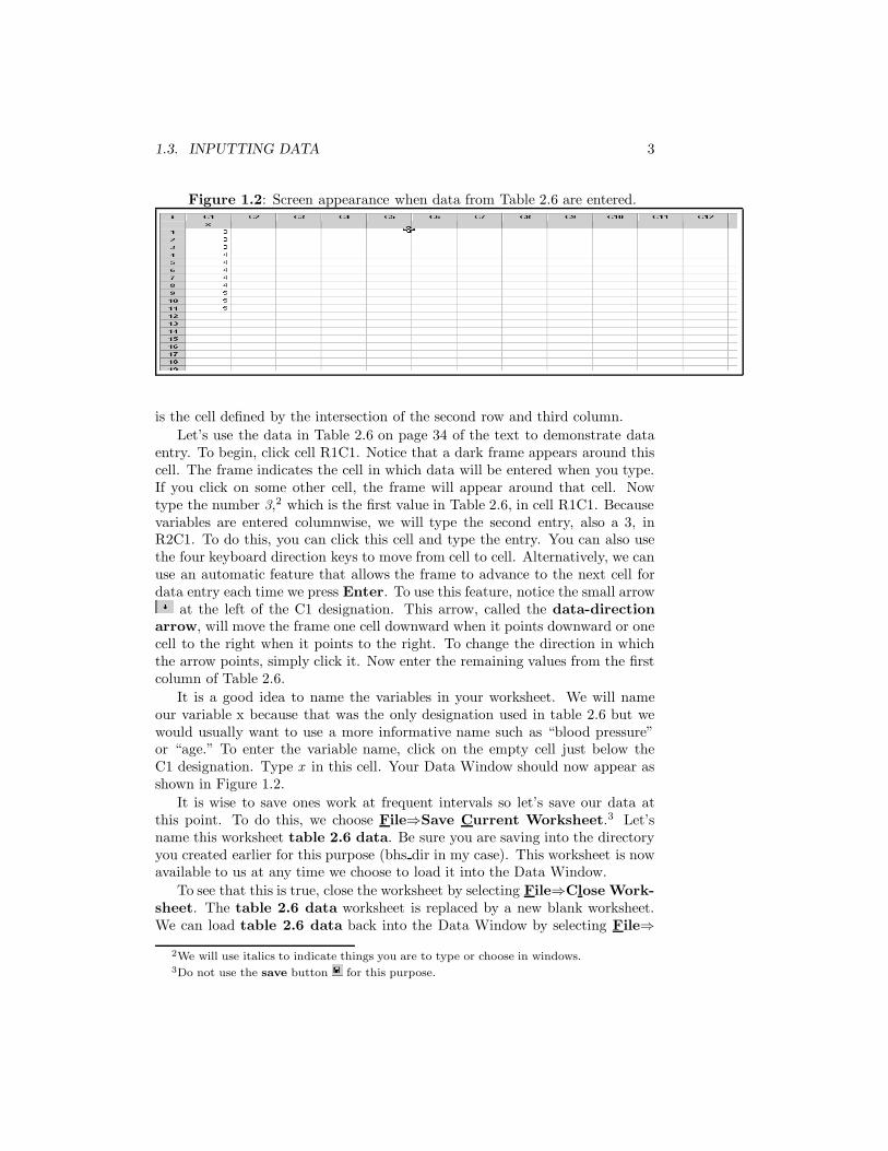
Figure 1.2: Screen appearance when data from Table 2.6 are entered.
is the cell defined by the intersection of the second row and third column.Let’s use the data in Table 2.6 on page 34 of the text to demonstrate data
entry. To begin, click cell R1C1. Notice that a dark frame appears around thiscell. The frame indicates the cell in which data will be entered when you type.If you click on some other cell, the frame will appear around that cell. Nowtype the number 3,2 which is the first value in Table 2.6, in cell R1C1. Becausevariables are entered columnwise, we will type the second entry, also a 3, inR2C1. To do this, you can click this cell and type the entry. You can also usethe four keyboard direction keys to move from cell to cell. Alternatively, we canuse an automatic feature that allows the frame to advance to the next cell fordata entry each time we press Enter. To use this feature, notice the small arrow
at the left of the C1 designation. This arrow, called the data-directionarrow, will move the frame one cell downward when it points downward or onecell to the right when it points to the right. To change the direction in whichthe arrow points, simply click it. Now enter the remaining values from the firstcolumn of Table 2.6.
It is a good idea to name the variables in your worksheet. We will nameour variable x because that was the only designation used in table 2.6 but wewould usually want to use a more informative name such as “blood pressure”or “age.” To enter the variable name, click on the empty cell just below theC1 designation. Type x in this cell. Your Data Window should now appear asshown in Figure 1.2.
It is wise to save ones work at frequent intervals so let’s save our data atthis point. To do this, we choose File⇒Save Current Worksheet.3 Let’sname this worksheet table 2.6 data. Be sure you are saving into the directoryyou created earlier for this purpose (bhs dir in my case). This worksheet is nowavailable to us at any time we choose to load it into the Data Window.
To see that this is true, close the worksheet by selecting File⇒Close Work-sheet. The table 2.6 data worksheet is replaced by a new blank worksheet.We can load table 2.6 data back into the Data Window by selecting File⇒
2We will use italics to indicate things you are to type or choose in windows.3Do not use the save button for this purpose.

4 CHAPTER 1. PRELIMINARIES
Open Worksheet..., and choosing table 2.6 data.MTW from the file list.Note that MINITAB has appended the suffix MTW to the file. Now click Openand table 2.6 data.MTW reappears in the Data Window.
1.4 Performing Analyses
Now that we have entered our data, we can use MINITAB to perform analyseson these data. We will provide a simple example in this section but will givenumerous examples in the chapters that follow.
MINITAB uses two methods for performing analyses and other tasks. Thefirst is menu driven while the second makes use of Session commands. We willcover only the use of menus for analyses in this manual. To learn the Sessioncommand method, consult the MINITAB Handbook (see footnote 1 on page i).
Before beginning the analysis, be sure your data are displayed. If they arenot displayed,4 select File⇒Open Worksheet..., navigate to the directory inwhich you saved table 2.6 data and open it.
Let’s begin by calculating a few descriptive statistics on the variable we’velabeled x. To do this, select Stat⇒Basic Statistics⇒Display DescriptiveStatistics.... A window opens. You can determine which statistics will bedisplayed by selecting Statistics.... If you select this option, a window openslisting all the statistics that may be displayed with this command. Those thatare checked will be displayed. Close this window by selecting OK or Cancel.
Though you only have one variable (x) in this data set, you will often havemore. For this reason, you must tell MINITAB which variable(s) you wish toenter into the analysis. You can de this by double-clicking on x in the left handwindow or typing x into the Variables: window. You can also enter the columnnumber (C1 in this case). It is important to remember that names containing aspace must be enclosed in single quotes. MINITAB will put these quotes aroundthe variable name for you if you use the double-click method for entering thevariable name into the Variables: window. Your screen appears as in Figure1.3. Now select OK to perform the analysis.
Because we didn’t change any of the statistics in the Statistics... window,results are displayed in the Session Window as shown in Figure 1.4. Displayedthere are (a) the variable name (x), (b) the number of variable observations(11), (c) the number of missing variable observations (0), (d) the mean of x(4.000), (e) the standard error of the mean (0.234), (f) the standard deviationof x (0.775), (g) the minimum value of x (3.000), (h) the first quartile (3.000), (i)the median (4.000), (j) the third quartile (5.000) and, (k) the maximum value ofx (5.000). You will learn about each of these in your text. If other statistics werechecked in the Statistics... window you will have these statistics displayed.
4Your data will not be displayed if you’ve ended the MINITAB session or closed the work-sheet.

1.4. PERFORMING ANALYSES 5
Figure 1.3: Screen appearance for display of basicstatistics.
Figure 1.4: Display of basic statistics from x variable in text Table 2.6.

6 CHAPTER 1. PRELIMINARIES
Figure 1.5: Edited output of basic statistics from x variable in textTable 2.6.
1.5 Editing and Printing Your Output
Once you have produced output in the Session Window, you will likely want toedit and/or print it. For example, you may wish to add your name, date and aclass assignment number. You may then want to print out the result to turn into your instructor.
To begin, be sure your editor is set to allow editing of output. To do this,click anywhere in the Session Window. (You can easily move from the DataWindow to the Session Window and visa versa by simply clicking in the desiredwindow.) Then select Editor. If, in the list of options, Output Editable hasa check mark by it, the output is already amenable for editing and you needdo nothing more. If not, click by this option to place a check mark there. Youcan now carry out routine editing tasks such as typing, highlighting, cutting,copying, pasting etc. You can also cut and copy portions of the output toMicrosoft Word r© or other word processors if you so desire. If you wish to printportions of the output, simply highlight the part you want to print and use theusual printing commands. Figure 1.5 shows our edited output.
1.6 Using the Calculator
From time to time you may wish to use the variables in your data set to createnew variables. This can be done through use of the calculator provided byMINITAB. To demonstrate its use, let’s use it to create the second column inTable 2.6 which, as you can see, is the square of the first column.
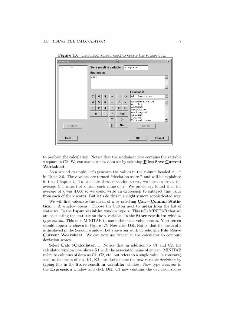
To begin, be sure that table 2.6 data.MTW is the current worksheet.Then select Calc⇒Calculator.... The Calculator window opens. In the Storeresult in variable: window type x square. This will be the name of the newvariable which will be placed in the next available column which is C2 in thiscase. In the Expression: window type x**2. The symbol “**” means “raiseto the power of”. Had we typed “x**3” the new variable would be the cubeof x. Thus, what we have typed in this case is equivalent to “x square=x**2.”Figure 1.6 shows the calculator screen used for the calculation. Now click OK
1.6. USING THE CALCULATOR 7
Figure 1.6: Calculator screen used to create the square of x.
to perform the calculation. Notice that the worksheet now contains the variablex square in C2. We can save our new data set by selecting File⇒Save CurrentWorksheet.
As a second example, let’s generate the values in the column headed x − xin Table 2.6. These values are termed “deviation scores” and will be explainedin text Chapter 2. To calculate these deviation scores, we must subtract theaverage (i.e. mean) of x from each value of x. We previously found that theaverage of x was 4.000 so we could write an expression to subtract this valuefrom each of the x scores. But let’s do this in a slightly more sophisticated way.
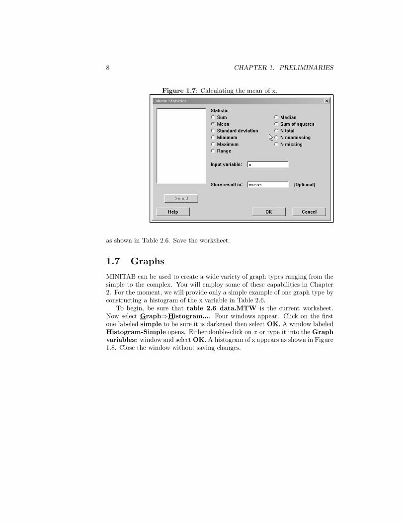
We will first calculate the mean of x by selecting Calc⇒Column Statis-tics.... A window opens. Choose the button next to mean from the list ofstatistics. In the Input variable: window type x. This tells MINITAB that weare calculating the statistic on the x variable. In the Store result in: windowtype xmean. This tells MINITAB to name the mean value xmean. Your screenshould appear as shown in Figure 1.7. Now click OK. Notice that the mean of xis displayed in the Session window. Let’s save our work by selecting File⇒SaveCurrent Worksheet. We can now use xmean in the calculator to computedeviation scores.
Select Calc⇒Calculator.... Notice that in addition to C1 and C2, thecalculator window now shows K1 with the associated name of xmean. MINITABrefers to columns of data as C1, C2, etc. but refers to a single value (a constant)such as the mean of x as K1, K2, etc. Let’s name the new variable deviation bytyping this in the Store result in variable: window. Now type x-xmean inthe Expression window and click OK. C3 now contains the deviation scores
8 CHAPTER 1. PRELIMINARIES
Figure 1.7: Calculating the mean of x.
as shown in Table 2.6. Save the worksheet.
1.7 Graphs
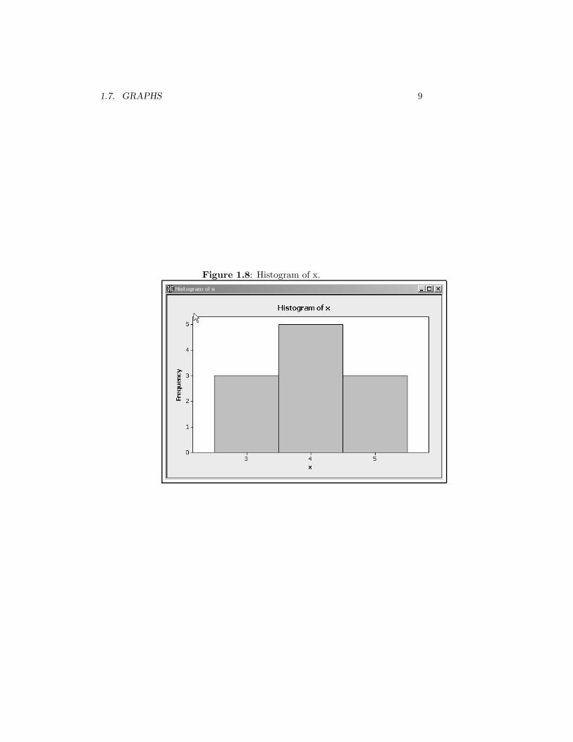
MINITAB can be used to create a wide variety of graph types ranging from thesimple to the complex. You will employ some of these capabilities in Chapter2. For the moment, we will provide only a simple example of one graph type byconstructing a histogram of the x variable in Table 2.6.
To begin, be sure that table 2.6 data.MTW is the current worksheet.Now select Graph⇒Histogram.... Four windows appear. Click on the firstone labeled simple to be sure it is darkened then select OK. A window labeledHistogram-Simple opens. Either double-click on x or type it into the Graphvariables: window and select OK. A histogram of x appears as shown in Figure1.8. Close the window without saving changes.
1.7. GRAPHS 9
Figure 1.8: Histogram of x.

10 CHAPTER 1. PRELIMINARIES
Figure 1.9: Reconstruction of Table 2.6.
Exercises
1.1 Use the Calculator... to construct the remaining variables in Table 2.6.The result should appear as in Figure 1.9. (Hint: double-clicking on afunction in the Functions: window places it in the Expression: window.
1.2 Use Display Descriptive Statistics... to find the means of all the vari-ables in Table 2.6. Don’t generate any other statistics. Use Display De-scriptive Statistics... only once. (Hint: You can place multiple variablesin the Variables window by double-clicking on each.
1.3 Label the output from Exercise 1.2 with your name and the current date.Print out the result.
1.4 Enter the data from text Table 7.1 into a new worksheet. Save the worksheetwith the name table 7.1 data.
1.5 Find the means of the three diet groups in Table 7.1. Label them meanone, mean two and mean three. Save them in the table 7.1 data work-sheet. (Don’t forget that names containing spaces must be enclosed in singlequotes.)
Chapter 2
Descriptive Methods
2.1 Introduction
In this chapter you will learn to use MINITAB to construct the graphs and cal-culate most of the statistics presented in text Chapter 2. You will also learn thatin a few instances MINITAB and the text do not agree on the calculated valuesof certain descriptive statistics because different definitions of these statisticsare used by the software and text. You will also be afforded an opportunity topractice data entry and data transformations.
2.4 Distributions (page 15)
Task 2.1
Use the data in Table 2.1 (table 2.1 data.MTW) to construct frequency,relative frequency, cumulative frequency, and cumulative relative frequency dis-tributions as shown in Table 2.2.
Solution
Load the worksheet containing the Table 2.1 data by selecting File⇒OpenWorksheet... and opening file table 2.1 data.MTW. Note first that thePain Level variable is expressed in text rather than numeric form. Because thecumulative frequency and cumulative relative frequency distributions requirethat the Pain Level variable be ordered, we must inform MINITAB as to thelow to high ordering of this variable before we can form these distributions.To do this, right-click on the Pain Level variable in the worksheet. A series ofchoices is displayed. Select Column⇒Value Order. A window opens. Selectthe option button for User specified Order:. New Order is automaticallyhighlighted in the Choose an order: window. The text values appear in awindow labeled Define an order (one value per line):. Place these values in
11
12 CHAPTER 2. DESCRIPTIVE METHODS
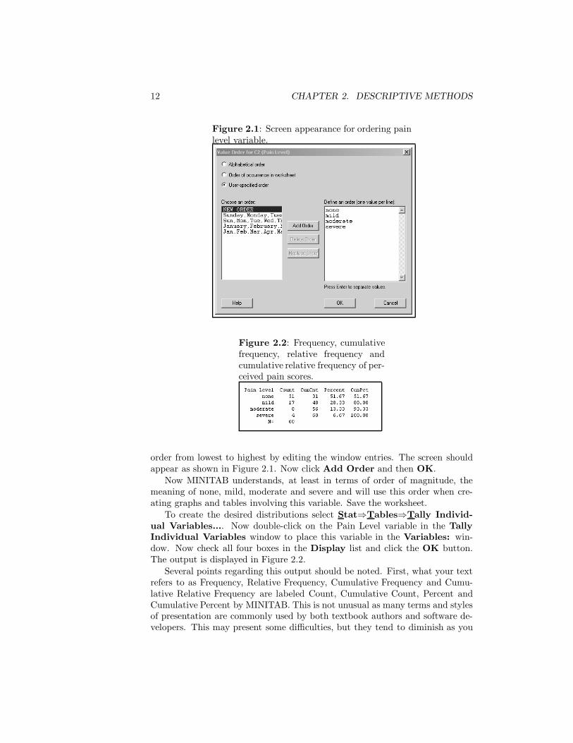
Figure 2.1: Screen appearance for ordering painlevel variable.
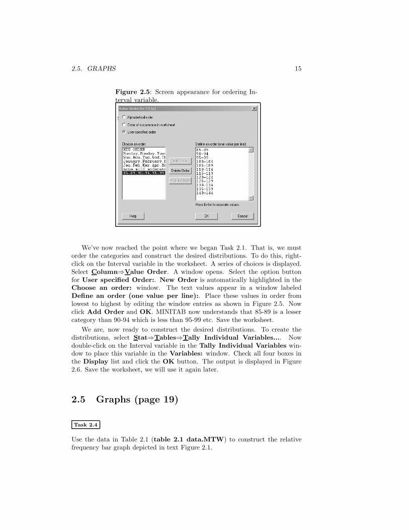
Figure 2.2: Frequency, cumulativefrequency, relative frequency andcumulative relative frequency of per-ceived pain scores.
order from lowest to highest by editing the window entries. The screen shouldappear as shown in Figure 2.1. Now click Add Order and then OK.
Now MINITAB understands, at least in terms of order of magnitude, themeaning of none, mild, moderate and severe and will use this order when cre-ating graphs and tables involving this variable. Save the worksheet.
To create the desired distributions select Stat⇒Tables⇒Tally Individ-ual Variables.... Now double-click on the Pain Level variable in the TallyIndividual Variables window to place this variable in the Variables: win-dow. Now check all four boxes in the Display list and click the OK button.The output is displayed in Figure 2.2.
Several points regarding this output should be noted. First, what your textrefers to as Frequency, Relative Frequency, Cumulative Frequency and Cumu-lative Relative Frequency are labeled Count, Cumulative Count, Percent andCumulative Percent by MINITAB. This is not unusual as many terms and stylesof presentation are commonly used by both textbook authors and software de-velopers. This may present some difficulties, but they tend to diminish as you

2.4. DISTRIBUTIONS 13
Figure 2.3: Simple frequencydistribution of BP scores asshown in Table 2.3.
gain more experience with different software packages. Second, with the ex-ception that MINITAB uses percents where the text uses proportions and thenumber of decimal places reported, the distributions provided by MINITAB arethe same as those in text Table 2.2. Third, MINITAB orders the distributionsin descending order while the text uses an ascending order. The style used byMINITAB is the more common. The text authors prefer the ascending orderingbut either is correct and provides the same information.
Task 2.2
Use the data in worksheet table 2.3 data.MTW to construct the simple fre-quency distribution depicted in the text Table 2.3.
Solution
Because the blood pressure data in worksheet table 2.3 data.MTW are nu-meric as opposed to text, we need not go through the process of defining thevariable order as was necessary with Task 2.1. Thus, we can construct thesimple frequency distribution without any preliminaries.
After loading table 2.3 data.MTW we select Stat⇒Tables⇒Tally In-dividual Variables..., then double-click on BP to place it in the Variables:window. Place a check by Counts in the Display window and remove anychecks by any other options in this list. Now select OK to produce the fre-quency distribution. The resultant frequency distribution is shown in Figure2.3. Note that I have edited the output into three columns to save page space.
Task 2.3
Use the data in worksheet table 2.3 data.MTW to construct the groupeddistributions depicted in the text Table 2.4.

14 CHAPTER 2. DESCRIPTIVE METHODS
Figure 2.4: Partial conversion table used to relate BP values to group inter-vals.
Solution
Unfortunately, MINITAB does not provide internal methods for constructinggrouped distributions. So, in order to complete this task, we must first code thenumeric values in table 2.3 data.MTW to form the discrete intervals shownin text Table 2.4. Because these categories are text based (even though theycontain numbers) we will follow the same procedure used for Task 2.1 to orderthe text categories. We will then be able to construct the desired distributionsas with previous tasks.
To begin the coding, we construct a conversion table that relates all BPvalues to specific category intervals. We will use C2 and C3 in our worksheetfor this purpose. For convenience, let’s label C2 as x and C3 as y. We now listall possible values of BP in x and the categories to which they relate in y. The(partial) result is shown in Figure 2.4.
We are now ready to use the conversion table to create the Interval vari-able. To accomplish this, select Data⇒Code⇒Use Conversion Table....The Code-Use Conversion Table window opens. Enter BP in the Inputcolumn: window. This tells MINITAB that it is the BP values that are to beconverted into intervals. Now type Interval in the Output column: window.This names the new variable “Interval.” Now type x in the Column of Orig-inal Values: window and y in the Column of New Values: window. Thistells MINITAB the values of BP that correspond to the specified intervals. Nowclick OK. A new variable, named Interval, consisting of the specified intervalsis created and placed in column C4 of the worksheet. Notice that each BP valueis related to its corresponding interval.
2.5. GRAPHS 15
Figure 2.5: Screen appearance for ordering In-terval variable.
We’ve now reached the point where we began Task 2.1. That is, we mustorder the categories and construct the desired distributions. To do this, right-click on the Interval variable in the worksheet. A series of choices is displayed.Select Column⇒Value Order. A window opens. Select the option buttonfor User specified Order:. New Order is automatically highlighted in theChoose an order: window. The text values appear in a window labeledDefine an order (one value per line):. Place these values in order fromlowest to highest by editing the window entries as shown in Figure 2.5. Nowclick Add Order and OK. MINITAB now understands that 85-89 is a lessercategory than 90-94 which is less than 95-99 etc. Save the worksheet.
We are, now ready to construct the desired distributions. To create thedistributions, select Stat⇒Tables⇒Tally Individual Variables.... Nowdouble-click on the Interval variable in the Tally Individual Variables win-dow to place this variable in the Variables: window. Check all four boxes inthe Display list and click the OK button. The output is displayed in Figure2.6. Save the worksheet, we will use it again later.
2.5 Graphs (page 19)
Task 2.4
Use the data in Table 2.1 (table 2.1 data.MTW) to construct the relativefrequency bar graph depicted in text Figure 2.1.

16 CHAPTER 2. DESCRIPTIVE METHODS
Figure 2.6: Grouped frequencydistributions for BP variable in12 categories.
Figure 2.7: Bar graph of pain level scores.
Solution
Open table 2.1 data.MTW as the active worksheet. Select Graph⇒BarChart.... If the bar chart in the window labeled “Simple” is not selected, clickon that window to select it and click OK. The Bar Chart-Counts of uniquevalues, Simple window opens. Double-click on Pain Level to place it in theCategorical variables: window. Because the task specified that a relativefrequency bar graph is to be constructed, we must inform MINITAB that thebars are to be shown in terms of proportions (or percents in this case). Todo this, select Bar Chart Options... and place a check in the Show Y aspercent box and click OK. You are now back at the Bar Chart-Counts ofunique values, Simple window. Click OK. The graph appears as shown inFigure 2.7. Print this graph by selecting File⇒Print Graph.
MINITAB allows graphs to be edited if so desired. As one example, supposewe wish the title of the graph to be “Bar Chart of Pain Level” rather than

2.5. GRAPHS 17
Figure 2.8: Informing MINITAB that a rela-tive frequency histogram is to be constructed.
simply “Chart of Pain Level.” Just double-click on Chart of Pain Level at thetop of the graph. The Edit Title window opens. Be sure the Font tab isselected. Now type in the desired title in the Text: window and click OK.The graph appears with the new title. You should experiment a bit to see whatother alterations you can make to the graph.
Notice that the pain levels are ordered. How do you think MINITAB knewthe order of this variable? (Hint: go back and look at Task 2.1.)
Task 2.5
Use the data in Table 2.3 (table 2.3 data.MTW) to construct the relativefrequency histogram depicted in text Figure 2.2.
Solution
Be sure table 2.3 data.MTW is the active worksheet. Then select Graph⇒Histogram.... The Histograms window opens. Select the Simple histogramby clicking on the depiction in the Simple window. Click on OK. In theHistogram-Simple window, double-click on BP to move this variable into theGraph variables: window. If we wished to construct a (default) frequencyhistogram we would click OK at this point and continue, but because we wishto form a relative frequency histogram we must inform MINITAB that this isthe case. To do so, select Scale... in the Histogram-Simple window. Thenchoose the Y-Scale Type tab and then click the Percent option. Your screenshould appear as in Figure 2.8. Now click OK then click OK again. A relativefrequency1 histogram appears but it is not grouped as in text Figure 2.2.
1Once again, MINITAB expresses the relative frequency as a percent rather than as aproportion as is done in the text. This will generally be the case so we will not continue to

18 CHAPTER 2. DESCRIPTIVE METHODS
Figure 2.9: Specifying intervals for arelative frequency histogram.
To form the appropriate grouping, double-click anywhere along the horizon-tal (i.e. x) axis of the histogram. The Edit Scale window opens. Choose theScale tab and darken the Position of ticks: button. Remove any entries inthe associated window and enter 84.5:144.5/5. Click the Binning tab. ChooseCutpoint in the Interval Type list. This tells MINITAB to label the intervalrather than the midpoint for each bar. Now choose Midpoint/Cutpoint posi-tions. In the accompanying window you could type 84.5 89.5 94.5 etc. to labelthe graph but MINITAB provides a shortcut that will be easier in this case.Type 84.5:144.5/5 in the window. This provides MINITAB with the range ofvalues for the x axis (84.5 to 144.5) as well as the interval size (5). The screenappears as in Figure 2.9. Click OK and the histogram depicted in Figure 2.10appears.
Task 2.6
Use the data in Table 2.3 (table 2.3 data.MTW) to construct the relativefrequency polygon depicted in text Figure 2.4.
Solution
This task can be approached in essentially the same manner as was used withTask 2.5 with the major difference being that we will ask MINITAB to pro-vide connected dots rather than bars in the depiction. To this end, selectGraph⇒Histogram.... Choose the Simple histogram and click OK. In theHistogram-Simple window double-click on the BP variable to place it in theGraph-variables: window if it isn’t there already. Now select Scale... and inthe Histogram-Scale window choose the Y-Scale Type tab. Under this tabdarken the Percent button so that MINITAB will plot percents rather thanfrequencies. Click OK. You are now back in the Histogram-Simple window.
remind you of this fact.

2.5. GRAPHS 19
Figure 2.10: MINITAB rendering of the histogram de-picted in text Figure 2.2.
From this window select Data View.... Under the Data Display tab place acheck by Symbols and uncheck any other checks. Now select the Smoothertab. Choose the Lowess button in the Smoother list and set the Degree ofsmoothing to 0 (zero). This causes MINITAB to connect the dots with line seg-ments. Click OK then click OK again. A relative frequency polygon appears.But it does not reflect the twelve groupings.
Double-click anywhere along the x axis. The Edit Scale window opens.Under the Scale tab, choose the Position of ticks: button. In the accom-panying window type 84.5:144.5/5. This tells MINITAB to place the first tickmark at 84.5, the last at 144.5 and every five units in between. Now choose theBinning tab. Be sure that Midpoint is selected under Interval Type so thatthe polygon dots will be placed at the midpoints of the intervals. Now choosethe Midpoint/Cutpoint positions: button. We now enter the midpoints ofour desired intervals as 82:147/5 and click OK. The desired polygon appears.
Let’s edit the graph just a bit. Double-click on the Histogram of BP titleat the top of the graph. In the Text: box type Relative Frequency Polygon ofBlood Pressures in 12 Categories and click OK. The graph appears with thenew title. Now double-click on the BP designation at the bottom of the graph.Type Systolic Blood Pressure in the Text: box and click OK. The relativefrequency polygon appears as in Figure 2.11.
Task 2.7
Use the data in Table 2.3 (table 2.3 data.MTW) to construct the cumulativerelative frequency polygon depicted in text Figure 2.6.

20 CHAPTER 2. DESCRIPTIVE METHODS
Figure 2.11: MINITAB rendering of the polygondepicted in text Figure 2.4.
Solution
In formulating a solution for Task 2.3, we used a conversion table to assignsubjects to specified intervals. We will use this technique again here to groupsubjects into the 12 intervals depicted in Figure 2.6. More specifically, we willassign the value 84.5 to all subjects with blood pressures of 85, 86, 87, 88 or89, a value of 89.5 to all subjects with pressures of 90, 91, 92, 93 or 94 andso on with the five highest scale values being assigned 139.5. You will see theunderlying rationale shortly.
The conversion table employed for the solution of Task 2.3 consisted of twovariables which we named x and y. The first of these listed all possible bloodpressure values while the second indicated the interval to which each of theseshould be assigned. We will use the x variable again here but we will replacethe y variable with a new set of intervals.
Be sure that table 2.3 data.MTW is the current worksheet. If you saved itat the completion of Task 2.3, it should appear as in Figure 2.4 except that thevariable named Interval has been added in C4-T. Let’s clean up this worksheetby deleting the y and Interval variables. To do this, click and hold down themouse button on C3-T and drag across to C4-T. This will select (darken) thesetwo columns. Now select Edit⇒Delete Cells. The C3 and C4 columns arenow empty.
To construct the new conversion table begin by labeling the C3 column y.Now enter the interval values in y as shown in Figure 2.12. This table indicatesthat the blood pressures listed in x will be converted to the values specified iny. Now let’s perform the conversion.
Select Data⇒Code⇒Use Conversion Table.... The Code-Use Con-version Table window opens. Double-click on BP to place it in the Inputcolumn: window. This tells MINITAB that it is the blood pressure values that

2.5. GRAPHS 21
Figure 2.12: Specifying intervals for a cumulative relativefrequency polygon.
are being coded. Now type Interval in the Output column: window. Thistells MINITAB to name the new variable Interval. Place an x in the Column ofOriginal Values: window and a y in the Column of New Values: window.This tells MINITAB which x values correspond to which y values. Click OKand the Interval variable appears in C4.
Our strategy now involves calculating the cumulative relative frequency forthe Interval variable. To this end, select Stat⇒Tables⇒Tally IndividualVariables.... In the Tally Individual Variables window double-click on theInterval variable to place it in the Variables window. In the Display list puta check by Cumulative percents and uncheck any others that have a checkby them. Click OK. The resultant distribution appears in the Session Windowand is shown in Figure 2.13.
We must now paste this result into the worksheet. To accomplish this, clickand drag the cursor in the Session Window so as to select (darken) all of theoutput depicted in Figure 2.13. Now select Edit⇒Copy to copy the selectedportion of the Session Window to the clipboard. Now click and hold downthe mouse button on C5 in the worksheet and drag the cursor across to C6 sothat both the C5 and C6 columns are selected (darkened). Select Edit⇒PasteCells. Be sure that the Use spaces as delimiters button is selected and clickOK. The cumulative relative frequency distribution now appears in columns C5and C6 as shown in Figure 2.14.2
Let’s now round off the CumPct values to the nearest integer. To do this, se-lect Calc⇒Calculator.... Double-click CumPct to place it in the Store resultin variable: window. Place the cursor in the Expression: window and double-click on round in the Functions: window. (You will have to scroll down to findthis function.) This enters “ROUND(number, num digits)” in the Functions:
2You can paste this distribution in C1 and C2 of a new worksheet if you prefer.

22 CHAPTER 2. DESCRIPTIVE METHODS
Figure 2.13: Cu-mulative relativefrequency distri-bution for bloodpressure measuresin 12 intervals.
Figure 2.14: Worksheet after pasting the cu-mulative relative frequency distribution intocolumns C5 and C6.

2.5. GRAPHS 23
Figure 2.15: MINITAB rendering of the cumulativerelative frequency polygon depicted in text Figure2.6.
window. Edit this expression so it appears as ROUND(‘CumPct’,0). This tellsMINITAB to round off the CumPct variable to the nearest whole number. ClickOK and the CumPct values are rounded to the nearest whole number. We arenow ready (at last) to create the graph.
Choose Graph⇒Scatter Plot.... In the Scatterplots window choose theWith Connect Line figure and click OK. Put CumPct in the Y variableswindow and Interval 1 in the X variables window and click OK. The cumula-tive distribution is presented on the screen.
In order to have the x axis scale conform with the scale in Figure 2.6, double-click on the x axis of the graph. In the Edit Scale wondow choose the Positionof ticks: button. In the accompanying window type 84.5:144.5/5 which tellsMINITAB to label the x axis from 84.5 to 144.5 in five unit increments. ClickOK. The graph appears with the x axis properly scaled.
Finally, let’s bring the y scale down so that zero will be closer to the x axisas in Figure 2.6. Double-click on the y axis. In the Edit Scale window be surethat the Scale tab is selected. Under Scale Range uncheck Minimum: andtype .1 in the accompanying window. This puts the bottom of the y scale nearzero. Now click OK and the graph depicted in Figure 2.15 appears. Feel freeto edit the graph titles to make them more meaningful.
Task 2.8
Construct a stem-and-leaf-display for the blood pressure data in text Table 2.3.
Solution
Be sure that table 2.3 data.MTW is the current worksheet. Select Graph⇒Stem-and-leaf.... Double-click on BP to place it in the Graph variables... windowand click OK. A stem-and-leaf-display appears in the Session Window as shown

24 CHAPTER 2. DESCRIPTIVE METHODS
Figure 2.16: MINITAB rendering of astem-and-leaf display for the BP vari-able in text Table 2.3.
Figure 2.17: Edited MINITAB ren-dering of a stem-and-leaf display for theBP variable in text Table 2.3.
in Figure 2.16.Note that MINITAB divides leaves in half so that digits 0 through 4 are
placed on one line and 5 through 9 are placed on a second line. Also, thenumbers on the far left are what MINITAB refers to as the depth of the stem.This column gives the cumulative frequency from the top of the figure downand from the bottom of the figure up. The number in parentheses gives the leafcount for the row containing the median.
Unlike other graphs produced by MINITAB, stem-and-leaf-displays are notprovided in special graph windows but are printed in the Session Window. Thismeans that they can be edited with ordinary cut and paste methods. Figure2.17 shows the display after we’ve edited it to more closely conform with textFigure 2.7.
2.6 Numerical Methods (page 23)
Task 2.9
In text Example 2.4 on page 27 you are asked to find the median of the numbers3, 2, 0, 2, 1, 1, 2, and 2. Two different methods are used that produce twodifferent answers, namely, 2.00 and 1.75. It is argued that the better answer isprovided by the method that produces the median value of 1.75. What answeris provided by MINITAB?

2.6. NUMERICAL METHODS 25
Solution
We begin by entering the numbers in C1 of a new worksheet. Name the vari-able x. Select Stat⇒Basic Statistics⇒Display Descriptive Statistics...Double-click on x to place it in the Variables... window. Now click on Statis-tics.... Place a check by Median if there isn’t one there already. Uncheck allother statistics and click OK then click OK again. The answer provided in theSession Window is 2.00.
Task 2.10
Find the mean, median, and standard deviation of the data in the table asso-ciated with Example 2.7 on page 30. Is the median reported by MINITAB thesame as that reported in the text? Why do you think this is the case?
Solution
We will have to enter this data into a worksheet since none is provided. Thisprocess can be somewhat simplified when data are given in the form of a simplefrequency distribution as in this case.
Open a new worksheet, if necessary, by selecting File⇒New.... Be sureMINITAB Worksheet is highlighted and click OK. From the table on textpage 30 we notice that there are three 2.4s in the table. To enter these se-lect Calc⇒Make Patterned Data⇒Arbitrary Set of Numbers.... In theStore patterned data in: window type C1 to store the 2.4s in C1. Type 2.4in the Arbitrary set of numbers: window and 3 in the List each value<blank> times window. There should be a 1 in the List the whole se-quence <blank> times window. Thus, we have informed MINITAB to placethree 2.4 values in C1. Now click OK. Three values of 2.4 appear in C1.
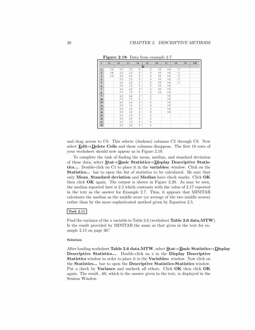
The next value in the table is 2.3 and there are 40 of those so we will place 402.3s in C2. To enter these select Calc⇒Make Patterned Data⇒ArbitrarySet of Numbers.... In the Store patterned data in: window type C2.Type 2.3 in the Arbitrary set of numbers: window and 40 in the List eachvalue <blank> times window. There should still be a 1 in the List thewhole sequence <blank> times window. Now click OK. C2 now contains40 2.3s. We continue this process by placing 36 2.2s in C3, 21 2.1s in C4, 182.0s in C5, 8 1.9s in C6, 14 1.8s in C7 and 5 1.7s in C8. The first 18 rows ofyour worksheet should appear as in Figure 2.18.
In order to perform analyses, we must form these eight columns into a singlecolumn variable. To do this, select Data⇒Stack⇒Columns.... Now double-click C1 through C8 in the Stack Columns window in order to enter thesecolumns in the Stack the following columns: window. Now choose theColumn of current worksheet button and enter C1 in the accompanyingwindow. This set of instructions tells MINITAB to stack the values in C1through C8 in C1. Now click OK. The values in C1 through C8 are nowentered into C1. Let’s clean up the worksheet by deleting C2 through C8 whichwe no longer need. To accomplish this, click on the C2 heading in column C2
26 CHAPTER 2. DESCRIPTIVE METHODS
Figure 2.18: Data from example 2.7.
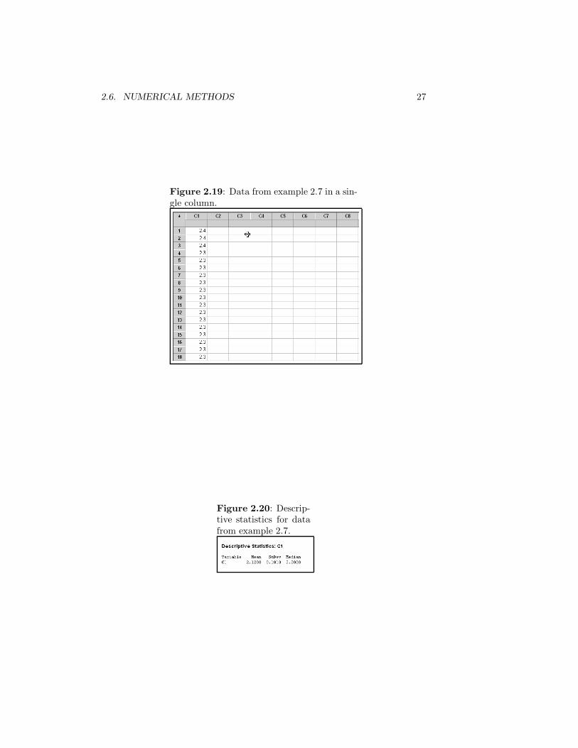
and drag across to C8. This selects (darkens) columns C2 through C8. Nowselect Edit⇒Delete Cells and these columns disappear. The first 18 rows ofyour worksheet should now appear as in Figure 2.19.
To complete the task of finding the mean, median, and standard deviationof these data, select Stat⇒Basic Statistics⇒Display Descriptive Statis-tics.... Double-click on C1 to place it in the variables: window. Click on theStatistics... bar to open the list of statistics to be calculated. Be sure thatonly Mean, Standard deviation and Median have check marks. Click OKthen click OK again. The output is shown in Figure 2.20. As may be seen,the median reported here is 2.2 which contrasts with the value of 2.17 reportedin the text as the answer for Example 2.7. Thus, it appears that MINITABcalculates the median as the middle score (or average of the two middle scores)rather than by the more sophisticated method given by Equation 2.5.
Task 2.11
Find the variance of the x variable in Table 2.6 (worksheet Table 2.6 data.MTW).Is the result provided by MINITAB the same as that given in the text for ex-ample 2.15 on page 36?
Solution
After loading worksheet Table 2.6 data.MTW, select Stat⇒Basic Statistics⇒DisplayDescriptive Statistics.... Double-click on x in the Display DescriptiveStatistics window in order to place it in the Variables: window. Now click onthe Statistics... bar to open the Descriptive Statistics-Statistics window.Put a check by Variance and uncheck all others. Click OK then click OKagain. The result, .60, which is the answer given in the text, is displayed in theSession Window.
2.6. NUMERICAL METHODS 27
Figure 2.19: Data from example 2.7 in a sin-gle column.
Figure 2.20: Descrip-tive statistics for datafrom example 2.7.
28 CHAPTER 2. DESCRIPTIVE METHODS
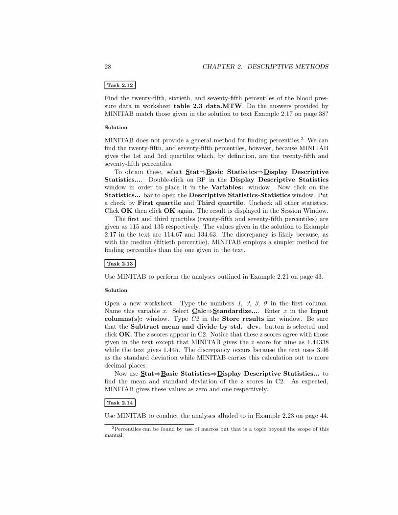
Task 2.12
Find the twenty-fifth, sixtieth, and seventy-fifth percentiles of the blood pres-sure data in worksheet table 2.3 data.MTW. Do the answers provided byMINITAB match those given in the solution to text Example 2.17 on page 38?
Solution
MINITAB does not provide a general method for finding percentiles.3 We canfind the twenty-fifth, and seventy-fifth percentiles, however, because MINITABgives the 1st and 3rd quartiles which, by definition, are the twenty-fifth andseventy-fifth percentiles.
To obtain these, select Stat⇒Basic Statistics⇒Display DescriptiveStatistics.... Double-click on BP in the Display Descriptive Statisticswindow in order to place it in the Variables: window. Now click on theStatistics... bar to open the Descriptive Statistics-Statistics window. Puta check by First quartile and Third quartile. Uncheck all other statistics.Click OK then click OK again. The result is displayed in the Session Window.
The first and third quartiles (twenty-fifth and seventy-fifth percentiles) aregiven as 115 and 135 respectively. The values given in the solution to Example2.17 in the text are 114.67 and 134.63. The discrepancy is likely because, aswith the median (fiftieth percentile), MINITAB employs a simpler method forfinding percentiles than the one given in the text.
Task 2.13
Use MINITAB to perform the analyses outlined in Example 2.21 on page 43.
Solution
Open a new worksheet. Type the numbers 1, 3, 3, 9 in the first column.Name this variable x. Select Calc⇒Standardize.... Enter x in the Inputcolumns(s): window. Type C2 in the Store results in: window. Be surethat the Subtract mean and divide by std. dev. button is selected andclick OK. The z scores appear in C2. Notice that these z scores agree with thosegiven in the text except that MINITAB gives the z score for nine as 1.44338while the text gives 1.445. The discrepancy occurs because the text uses 3.46as the standard deviation while MINITAB carries this calculation out to moredecimal places.
Now use Stat⇒Basic Statistics⇒Display Descriptive Statistics... tofind the mean and standard deviation of the z scores in C2. As expected,MINITAB gives these values as zero and one respectively.
Task 2.14
Use MINITAB to conduct the analyses alluded to in Example 2.23 on page 44.
3Percentiles can be found by use of macros but that is a topic beyond the scope of thismanual.

2.6. NUMERICAL METHODS 29
Solution
Open the table 2.8 data.MWS worksheet. The data for distributions A, B andC are in columns with the like letter. Select Stat⇒Basic Statistics⇒DisplayDescriptive Statistics.... Double-click A, B and C to place them in theVariables: window. Click Statistics... and place a check by skewness anduncheck all other statistics. Click OK and click OK again. Skew for the threedistributions is displayed in the Session Window. MINITAB reports skew forthe three distributions as 0.00, −0.77 and 0.77 while the solution for Example2.23 gives skew of zero, −.648, and .648. Because there are different definitionsof skew, it appears that MINITAB uses a different form than does the text. Thedefinition provided by the text is probably more common.
Task 2.15
Use MINITAB to perform the analyses outlined in Example 2.24 on page 46.
Solution
Open the table 2.9 data worksheet. Follow the same steps outlined in the so-lution to Task 2.14 with Kurtosis being checked rather than Skewness in theDescriptive Statistics-Statistics window. The values obtained for distribu-tions A and B respectively are 5.50 and −1.65 which differs markedly from thevalues of 5.04 and 1.26 given in the text. This again occurs because MINITABused a different definition of kurtosis than that used in the text. The definitiongiven in the text appears to be the more common.
30 CHAPTER 2. DESCRIPTIVE METHODS
Exercises
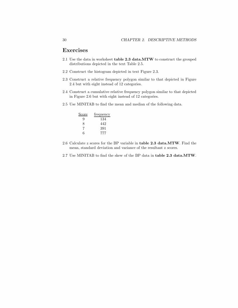
2.1 Use the data in worksheet table 2.3 data.MTW to construct the groupeddistributions depicted in the text Table 2.5.
2.2 Construct the histogram depicted in text Figure 2.3.
2.3 Construct a relative frequency polygon similar to that depicted in Figure2.4 but with eight instead of 12 categories.
2.4 Construct a cumulative relative frequency polygon similar to that depictedin Figure 2.6 but with eight instead of 12 categories.
2.5 Use MINITAB to find the mean and median of the following data.
Score frequency9 1348 4427 3916 777
2.6 Calculate z scores for the BP variable in table 2.3 data.MTW. Find themean, standard deviation and variance of the resultant z scores.
2.7 Use MINITAB to find the skew of the BP data in table 2.3 data.MTW.
Chapter 3
Probability
3.1 Introduction
In this chapter you will learn to use MINITAB to form contingency tables aswell as to find areas under the normal curve.
3.3 Contingency Tables (page 52)
Task 3.1
Use worksheet table 3.1 data.MWS to construct text Table 3.1 located onpage 54.
Solution
Notice that C1 of worksheet table 3.1 data.MWS characterizes each subjectas being a smoker (S) or a non-smoker (SN) while C2 characterizes each subjectas having some disease (D) or not having the disease (DN). In order to form thesedata into a contingency table, select Stat⇒Tables⇒Cross Tabulation andChi-Square.... Use double-clicks to enter Smoking Status in the For rows:window and Disease Status in the For columns: window. Check Countsin the Display list and click OK. The contingency table, with cell entries asdepicted in text Figure 3.1, appears in the Session Window.
3.4 The Normal Curve (page 62)
Task 3.2
Use MINITAB to find the area of the normal curve indicated in Example 3.9on page 64.
31

32 CHAPTER 3. PROBABILITY
Figure 3.1: MINITABrendering of Table 3.1.
Figure 3.2: Screen appearance for finding the area be-low 220 of a normal curve with mean 250 and standarddeviation 25.
Solution
MINITAB can find the area below any point on a normal distribution. To findthe indicated area for this task, select Calc⇒Probability Distributions⇒Normal....The Normal Distribution window opens. Be sure the Cumulative proba-bility button is selected. This tells MINITAB that the area below the specifiedvalue is to be calculated. Now enter the mean of 250 and standard deviation of25 in the appropriate windows. Be sure the Input constant: button is selectedand type 220 in the accompanying window. Your screen should appear as inFigure 3.2. Click OK and the area, 0.115070, appears in the Session Window.This agrees with the answer of .1151 given in the text.

Exercises 33
Exercises
3.1 Construct a worksheet to represent the data in the accompanying contin-gency table. Then use the worksheet to construct the contingency table.
B B
A 1 3 4A 3 3 6
4 6
3.2 Use MINITAB in lieu of the normal curve table (text Appendix A) to findthe areas of the normal curve indicated in Examples 3.10, 3.11 and 3.12.

34 CHAPTER 3. PROBABILITY

Chapter 4
Introduction to Inferenceand One Sample Methods
4.1 Introduction
In this chapter you will use MINITAB to find binomial probabilities as well asprobabilities associated with the normal curve. You will also learn to performvarious hypothesis tests, including equivalence tests, and form certain confidenceintervals. In addition, you will perform power calculations and compute requiredsample sizes to attain specified levels of power.
4.2 Sampling Distributions (page 75)
Task 4.1
Generate the binomial probabilities in Table 4.1 on page 83.
Solution
Enter the values 0 through 5 in C1 of a new worksheet. Then select Calc⇒ProbabilityDistributions⇒Binomial.... In the Binomial Distribution window selectthe Probability button. Type 5 in the Number of trials: window and .10in the Probability of success: window. Select the Input column: buttonand type C1 in the accompanying window. This tells MINITAB the number ofsuccesses for which probabilities are to be calculated. If you wish to have theprobabilities placed in C2, type C2 in the accompanying Optional storage:window or, if you prefer, leave this window blank and the probabilities will beprinted in the Session Window. Now click OK and the probabilities, as shownin Figure 4.1, appear in the Session Window.1
1Or in C2 if you chose that option.
35

36 CHAPTER 4. INFERENCE AND ONE SAMPLE METHODS
Figure 4.1: MINITAB ren-dering of binomial probabili-ties in Table 4.1.
Task 4.2
The Z value calculated in connection with Example 4.7 on page 86 was −5.33.Use MINITAB to find the associated probability.
Solution
Select Calc⇒Probability Distributions⇒Normal.... In the Normal Dis-tribution window be sure the Cumulative probability button is selected.This tells MINITAB to give us the proportion of the curve that lies below theindicated Z value. Now enter 0.0 and 1.0 for the mean and standard devia-tion respectively. This is because we are dealing with a distribution of Z scores(i.e. the standard normal curve) which has mean zero and standard deviationone. Select the Input constant: button and enter −5.33 in the accompanyingwindow and click OK. The result appears in the Session Window as 0.0000000.While the result cannot be exactly zero, it is zero to seven decimal places.
4.3 Hypothesis Testing (page 86)
Task 4.3
Use MINITAB to perform the one mean Z test outlined in Example 4.9 on page92.
Solution
Select Stat⇒Basic Statistics⇒1-Sample Z.... In the 1-Sample Z (Testand Confidence Interval) window select the Summarized data button.This tells MINITAB that you will supply the sample size and mean rather thanhaving MINITAB calculate it from a data sample. In the Sample size: windowtype 150 and in the Mean: window type 128.2. In the Standard deviation:window type 40 then type 120 in the Test mean: window. We must nowinform MINITAB as to the nature of the alternative hypothesis. To do this,select Options... and in the Alternative: window select greater than. Nowclick OK and click OK again. MINITAB displays obtained Z of 2.51 with

4.3. HYPOTHESIS TESTING 37
a one-tailed p-value of .006. Both numbers agree with those reported in thesolution to Example 4.9.
Normally, we would not bother performing the critical Z versus obtained Zversion of the test but in the spirit of learning more about MINITAB we will nextfind critical Z. To do this select Calc⇒Probability Distributions⇒Normal....Select the Inverse cumulative probability button in the Normal Distribu-tion window. This tells MINITAB that you want a Z value defined by having aspecified proportion of the normal curve lying below it. Because we are dealingwith a one-tailed test with alternative of the form HA : µ > 120 and α = .01,the desired Z value cuts off .01 in the upper tail of the curve which means that.99 of the curve lies below it. Choose the Input constant: button and enter.99 in the accompanying window. Be sure the Mean: and Standard devia-tion: are specified as 0.0 and 1.0 respectively and click OK. MINITAB givescritical Z (labeled X in the output) as 2.32635 which agrees with that given inthe solution to Example 4.9.
Task 4.4
Use MINITAB to perform the one mean Z test outlined in Example 4.12 onpage 97.
Solution
Select Stat⇒Basic Statistics⇒1-Sample Z.... In the 1-Sample Z (Testand Confidence Interval) window select the Summarized data button.This tells MINITAB that you will supply the sample size and mean rather thanhaving MINITAB calculate it from a data sample. In the Sample size: windowtype 40 and in the Mean: window type 87.1. In the Standard deviation:window type 21 then type 80 in the Test mean: window. We must nowinform MINITAB as to the nature of the alternative hypothesis. To do this,select Options... and in the Alternative: window select not equal whichspecifies a two-tailed test. Now click OK and click OK again. MINITABdisplays obtained Z of 2.14 with a two-tailed p-value of 0.032. Both numbersagree with those reported in the solution to Example 4.12.
To find critical Z, select Calc⇒Probability Distributions⇒Normal....Select the Inverse cumulative probability button in the Normal Distribu-tion window. This tells MINITAB that you want a Z value defined by having aspecified proportion of the normal curve lying below it. Because we are dealingwith a two-tailed test with α = .10, one of the desired Z values cuts off .05in the upper tail of the curve which means that .95 of the curve lies below it.Choose the Input constant: button and enter .95 in the accompanying win-dow. Be sure the Mean: and Standard deviation: are specified as 0.0 and1.0 respectively and click OK. MINITAB gives critical Z as 1.64485. Becausethe test is two-tailed we know the critical values are ±1.64485 which, with theexception of the number of decimal places employed, agrees with those given inthe solution to Example 4.12.2
2Note that 1.64485 rounds to 1.64 when rounded to two decimal places. However, the value
38 CHAPTER 4. INFERENCE AND ONE SAMPLE METHODS
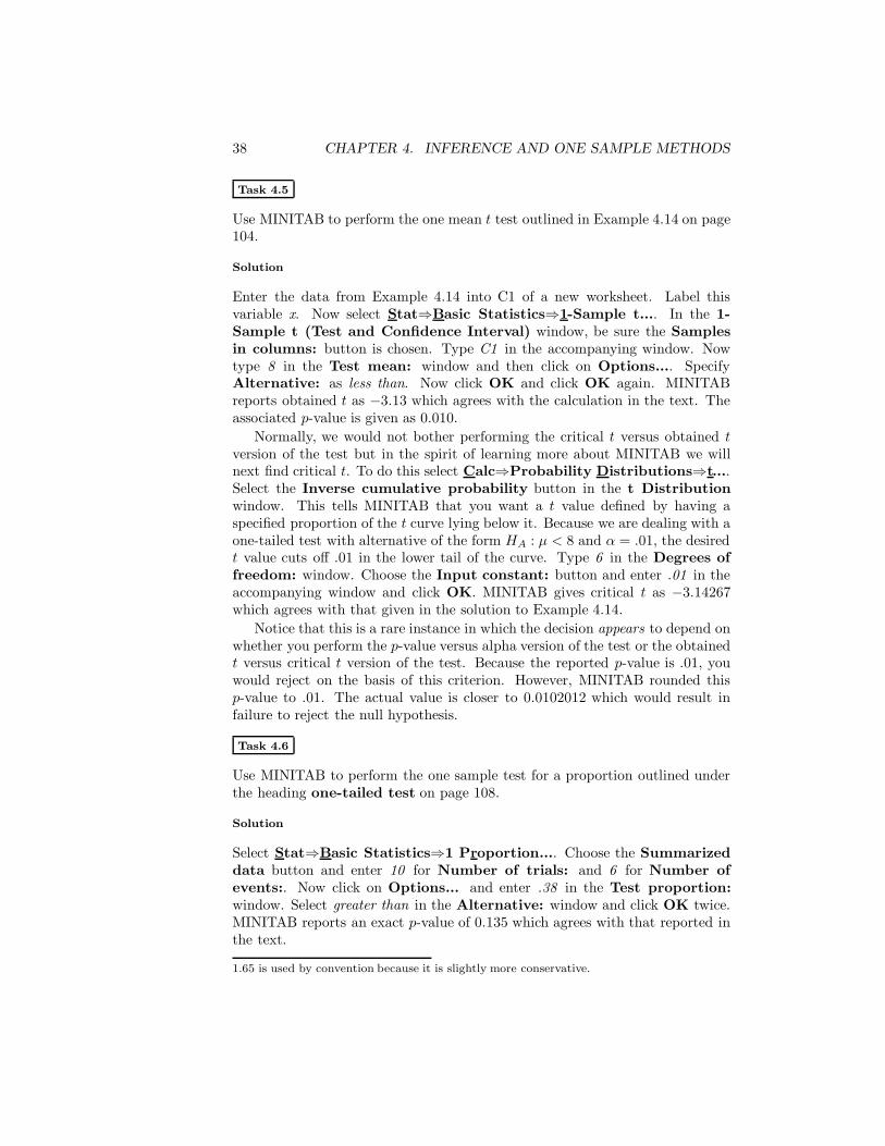
Task 4.5
Use MINITAB to perform the one mean t test outlined in Example 4.14 on page104.
Solution
Enter the data from Example 4.14 into C1 of a new worksheet. Label thisvariable x. Now select Stat⇒Basic Statistics⇒1-Sample t.... In the 1-Sample t (Test and Confidence Interval) window, be sure the Samplesin columns: button is chosen. Type C1 in the accompanying window. Nowtype 8 in the Test mean: window and then click on Options.... SpecifyAlternative: as less than. Now click OK and click OK again. MINITABreports obtained t as −3.13 which agrees with the calculation in the text. Theassociated p-value is given as 0.010.
Normally, we would not bother performing the critical t versus obtained tversion of the test but in the spirit of learning more about MINITAB we willnext find critical t. To do this select Calc⇒Probability Distributions⇒t....Select the Inverse cumulative probability button in the t Distributionwindow. This tells MINITAB that you want a t value defined by having aspecified proportion of the t curve lying below it. Because we are dealing with aone-tailed test with alternative of the form HA : µ < 8 and α = .01, the desiredt value cuts off .01 in the lower tail of the curve. Type 6 in the Degrees offreedom: window. Choose the Input constant: button and enter .01 in theaccompanying window and click OK. MINITAB gives critical t as −3.14267which agrees with that given in the solution to Example 4.14.
Notice that this is a rare instance in which the decision appears to depend onwhether you perform the p-value versus alpha version of the test or the obtainedt versus critical t version of the test. Because the reported p-value is .01, youwould reject on the basis of this criterion. However, MINITAB rounded thisp-value to .01. The actual value is closer to 0.0102012 which would result infailure to reject the null hypothesis.
Task 4.6
Use MINITAB to perform the one sample test for a proportion outlined underthe heading one-tailed test on page 108.
Solution
Select Stat⇒Basic Statistics⇒1 Proportion.... Choose the Summarizeddata button and enter 10 for Number of trials: and 6 for Number ofevents:. Now click on Options... and enter .38 in the Test proportion:window. Select greater than in the Alternative: window and click OK twice.MINITAB reports an exact p-value of 0.135 which agrees with that reported inthe text.
1.65 is used by convention because it is slightly more conservative.
4.3. HYPOTHESIS TESTING 39
Task 4.7
Use MINITAB to perform the one sample test for a proportion outlined inExample 4.19 on page 113.
Solution
Select Stat⇒Basic Statistics⇒1 Proportion.... Choose the Summarizeddata button and enter 8 for Number of trials: and 2 for Number of events:.Now click on Options... and enter .35 in the Test proportion: window. Se-lect not equal in the Alternative: window and click OK twice. MINITABreports an exact p-value of 0.721 which does not agree with the value of .85562reported in the text. This is because MINITAB uses a much more compli-cated method for finding the p-value for two-tailed tests based on the binomialdistribution.
Task 4.8
Use MINITAB to carry out the two-tailed equivalence test outlined in Example4.25 on page 120.
Solution
Begin by entering the sample data into C1 of a new worksheet. We can nowuse MINITAB to conduct two one-tailed t tests as is done in the text. However,there is a simpler way to establish two-tailed equivalence which we will alsodemonstrate.3 We begin by conducting the tests as was done in the text.
To conduct Test One select Stat⇒Basic Statistics⇒1 Sample t.... Besure the Samples in columns: button is selected and type C1 in the ac-companying window. Type 2 in the Test mean: window. Now click on theOptions... button and choose less than in the Alternative: window. ClickOK and click OK again. MINITAB reports obtained t in the Session Windowas −3.64 which agrees with the result given in the text. The reported p-valueis 0.003 which results in rejection of the null hypothesis.
Test Two is carried out in the same manner with -2 replacing 2 in theTest mean: window and greater than replacing less than in the Alternative:window. Obtained t is reported as 2.18 which agrees with that given in the text.The p-value is given as 0.028 which results in rejection of the null hypothesis.Because both tests are significant, the null hypothesis of non-equivalence isrejected in favor of the alternative of equivalence.
A much simpler way of conducting a two-tailed equivalence test4 is by form-ing a 100 (1 − 2α) percent confidence interval and noting the relationship ofL and U to EIL and EIU . If both L and U are between EIL and EIU , the
3The authors of your text presented two-tailed equivalence testing in the manner they didbecause they believed that, while more tedious, this method led to a better understanding ofthe equivalence concept.
4You may wish to delay learning this form of testing until you’ve studied Sections 4.4 and4.5.
40 CHAPTER 4. INFERENCE AND ONE SAMPLE METHODS
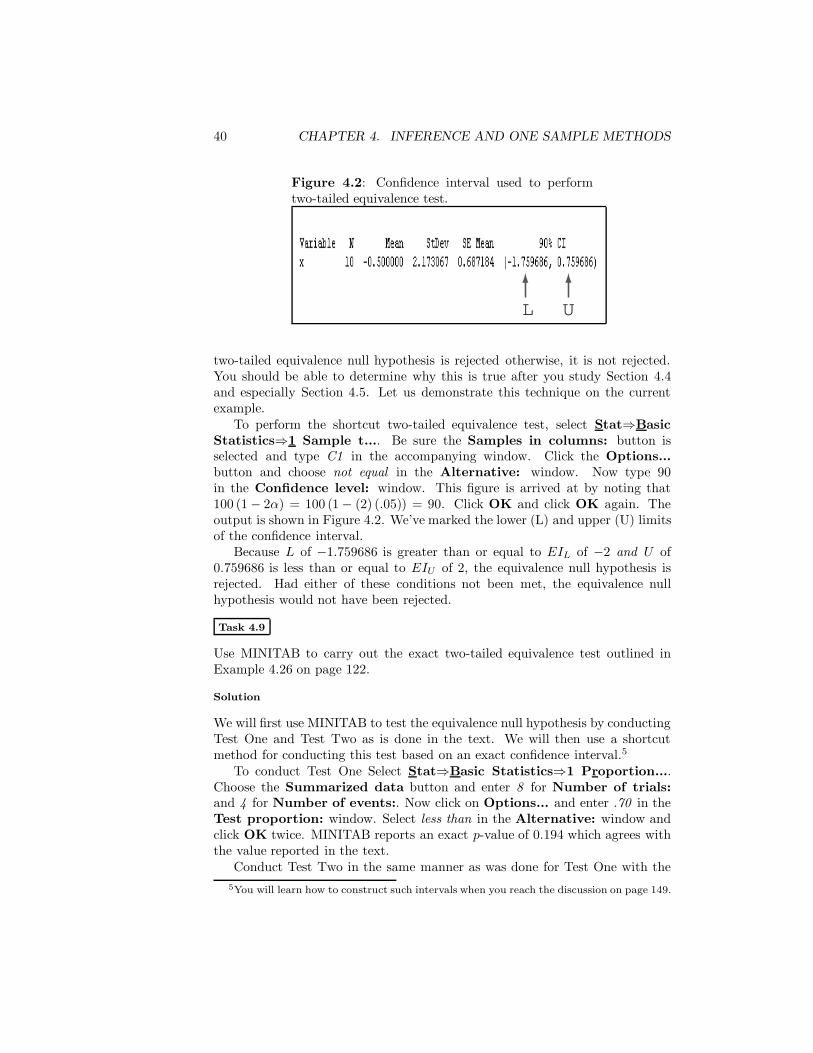
Figure 4.2: Confidence interval used to performtwo-tailed equivalence test.
L U
two-tailed equivalence null hypothesis is rejected otherwise, it is not rejected.You should be able to determine why this is true after you study Section 4.4and especially Section 4.5. Let us demonstrate this technique on the currentexample.
To perform the shortcut two-tailed equivalence test, select Stat⇒BasicStatistics⇒1 Sample t.... Be sure the Samples in columns: button isselected and type C1 in the accompanying window. Click the Options...button and choose not equal in the Alternative: window. Now type 90in the Confidence level: window. This figure is arrived at by noting that100 (1 − 2α) = 100 (1 − (2) (.05)) = 90. Click OK and click OK again. Theoutput is shown in Figure 4.2. We’ve marked the lower (L) and upper (U) limitsof the confidence interval.
Because L of −1.759686 is greater than or equal to EIL of −2 and U of0.759686 is less than or equal to EIU of 2, the equivalence null hypothesis isrejected. Had either of these conditions not been met, the equivalence nullhypothesis would not have been rejected.
Task 4.9
Use MINITAB to carry out the exact two-tailed equivalence test outlined inExample 4.26 on page 122.
Solution
We will first use MINITAB to test the equivalence null hypothesis by conductingTest One and Test Two as is done in the text. We will then use a shortcutmethod for conducting this test based on an exact confidence interval.5
To conduct Test One Select Stat⇒Basic Statistics⇒1 Proportion....Choose the Summarized data button and enter 8 for Number of trials:and 4 for Number of events:. Now click on Options... and enter .70 in theTest proportion: window. Select less than in the Alternative: window andclick OK twice. MINITAB reports an exact p-value of 0.194 which agrees withthe value reported in the text.
Conduct Test Two in the same manner as was done for Test One with the5You will learn how to construct such intervals when you reach the discussion on page 149.
4.3. HYPOTHESIS TESTING 41
exceptions that .30 is substituted for .70 in the Test proportion: windowand greater than is substituted for less than in the Alternative: window. Thereported p-value is again 0.194. Because both p-values are less than α = .20,the equivalence null hypothesis is rejected.
For the shortcut method, Select Stat⇒Basic Statistics⇒1 Proportion....Choose the Summarized data button and enter 8 for Number of trials: and4 for Number of events:. Now click on Options... and enter 100 (1− 2α) =100 (1 − (2) (20)) = 60 in the Confidence level: window. Now enter not equalin the Alternative: window and click OK twice. The reported confidenceinterval is (0.303226, 0.696774). Because this interval is completely containedin the equivalence interval of .3 to .7, the two-tailed equivalence null hypothesisis rejected.
Task 4.10
Compute power for the situation described in Example 4.32.
Solution
Select Stat⇒Power and Sample Size⇒1-Sample Z.... In the Power andSample Size for 1-Sample Z window, type 25 in the Sample sizes: windowand -2 in the Differences: window. This is the difference µ0 − µ. Be surethe Power values: window is blank. Type 20 in the Standard deviation:window then click the Options... button. Be sure the Not equal button isselected in the Alternative hypothesis list. Be sure the Significance level:is set to .05 and click OK twice. MINITAB gives the power calculation as0.0790975 which is slightly different from the value of .0721 calculated in thetext.
The discrepancy of .0790975−.0721 = .0069975 can be explained by referenceto Panel B of Figure 4.25 on page 134 of the text. In this figure power is depictedas the darkly shaded portion of the alternative curve that lies in the lower tailcritical region of the null curve. MINITAB adds to this figure the portion ofthe alternative curve that lies in the right hand critical region of the null curvethe reasoning being that this too would bring about rejection of the false nullhypothesis albeit for the wrong reason. That is, while µ < µ0, rejection in theright hand tail would lead one to believe that µ > µ0.6 We will leave calculationof the portion of the alternative curve that lies in the right hand critical regionof the null curve as an exercise.
Task 4.11
Use MINITAB to find the power alluded to in Example 4.34 on page 135.
Solution
We will begin by demonstrating a method that seems a natural way to proceed
6Some authors refer to this as a Type III error while others simply treat it as part of thepower calculation as does MINITAB.

42 CHAPTER 4. INFERENCE AND ONE SAMPLE METHODS
but provides poor results and then show how better results can be achieved. Tobegin, select Stat⇒Power and Sample Size⇒1 Proportion.... The Powerand Sample Size for 1 Proportion window appears. Type 8 in the Samplesizes: window, .5 in the Alternative values of p: window and .35 in theHypothesized p: window. Be sure the Power values: window is blank.
Now click Options... and choose the Greater than button. Type .05 inthe Significance level: window and click OK twice. Power is shown in theSession Window to be 0.235589 which is dramatically different from the valueof .14454 calculated in the text. The problem arises because MINITAB usesan approximate method based on the normal curve for its calculation while thecalculation in the text is exact. MINITAB will give us a better approximationif we replace the .05 entry in the Significance level: window with .02533which is the exact level of significance calculated in the text. When we do this,MINITAB gives the power estimate as 0.154862 which is much closer to thevalue of .14454 calculated in the text. The lesson to be learned here is that ifwe are using an exact test for a proportion, we should calculate and use theexact level of significance rather than simply inputting the intended level.
Task 4.12
Use MINITAB to calculate the sample size described in Example 4.36 on page136.
Solution
Select Stat⇒Power and Sample Size⇒1-Sample Z.... The Power andSample Size for 1-Sample Z window appears. Be sure the Sample sizes:window is blank. Type 2 in the Differences: window. This is the differenceµ0 − µ. Now type .8 in the Power values: window and 4 in the Standarddeviation: window. Click the Options... button and be sure the Not equalbutton is selected. Type .01 in the Significance level: window and click OKtwice. MINITAB prints the sample size of 47 in the Session Window which isthe solution calculated in t he text.
4.4 Confidence Intervals (page 137)
Task 4.13
Use MINITAB to construct the 95 percent confidence interval outlined in Ex-ample 4.37 on page 143.
Solution
Select Stat⇒Basic Statistics⇒1-Sample Z.... Select the Summarizeddata button in the 1-Sample Z (Test and Confidence Interval) window.Type 60 in the Sample size: window, 90.1 in the Mean: window and 16in the Standard deviation: window. Now click the Options... button. Be
4.4. CONFIDENCE INTERVALS 43
sure that the Confidence level: is set to 95.0 and the Alternative: is set tonot equal. Click OK twice. The interval, L = 86.0515 and U = 94.1485 areprovided in the Session Window. Both of these values agree with the resultsprovided in the text.
Task 4.14
Use MINITAB to construct the confidence interval described in Example 4.41on page 147.
Solution
Enter the data from Example 4.41 into C1 of a new worksheet. Select Stat⇒BasicStatistics⇒1-Sample t.... Select the Samples in columns: button and typeC1 in the accompanying window. Now click the Options... button and type99.0 in the Confidence level: window. Be sure not equal is selected in theAlternative: window and click OK twice. MINITAB gives the confidenceinterval as (94.654, 120.146) which agrees with the result given in the text.
Task 4.15
Use MINITAB to form the exact and approximate confidence intervals con-structed in Example 4.42 on page 150.
Solution
Select Stat⇒Basic Statistics⇒1 Proportion.... Select the Summarizeddata button. Enter 10 in the Number of trials: window and 4 in the numberof event: window. Click the Options... button. Be sure that 95.0 is entered inthe Confidence level: window and not equal is selected for the Alternative:window and click OK twice. MINITAB displays the confidence interval as(0.121552, 0.737622) which, given rounding, agrees with the exact computationscarried out in the text.
To obtain the approximate result, repeat the above steps but check the Usetest and interval based on normal distribution box under the Options...button. MINITAB gives the interval (0.096364, 0.703636) which, again, agreeswith the approximate interval given in the text. It is noteworthy that MINITABprovides the following admonition in association with this result. “* NOTE *The normal approximation may be inaccurate for small samples.”
44 CHAPTER 4. INFERENCE AND ONE SAMPLE METHODS
Exercises
4.1 Use MINITAB to reproduce the binomial probabilities in Table 4.5 on textpage 109 on page 143.
4.2 In Example 4.8 on page 86, the solution to the problem involves finding thearea of the normal curve that lies above a Z value of 1.36. The solutiongives this area as .0895. Use MINITAB and, if necessary a calculator, tofind this area.
4.3 Use MINITAB to perform the one mean Z test outlined in Example 4.11on page 95 as well as to find critical Z for the test.
4.4 Use MINITAB to perform the one mean Z test outlined in Example 4.13on page 98 as well as to find critical Z values for the test.
4.5 Use MINITAB to perform the one mean t test outlined in Example 4.16 onpage 106 as well as to find critical t for the test.
4.6 Use MINITAB to perform the test outlined in Example 4.18 on page 111.
4.7 Use MINITAB to perform the test outlined in Example 4.20 on page 114.
4.8 Use MINITAB to perform the following test of hypothesis using both themethod outlined in the text (i.e. Test One and Test Two) and the shortcut(i.e. confidence interval) method.
H0E : π ≤ .45 or π ≥ .55
HAE : .45 < π < .55
where p = .47 and n = 500. Use α = .05.
4.9 In reference to Example 4.32, calculate the portion of the alternative curvethat lies in the right hand critical region of the null curve thereby reconcil-ing the difference of approximately .0069975 between the power calculationprovided by MINITAB and that calculated in the text.
4.10 Use MINITAB to obtain a good estimate of the exact power calculated inExample 4.35.
4.11 Use MINITAB to form the confidence interval described in Example 4.38on page 144.
4.12 Use MINITAB to form the confidence intervals described in Example 4.39on page 144.
4.13 Use MINITAB to construct the confidence interval outlined in Exercise 4.22on page 157.
4.14 Use MINITAB to construct the two-sided and one-sided confidence intervalsalluded to in Example 4.43 on page 151.
Chapter 5
Paired Samples Methods
5.1 Introduction
In this chapter you will use MINITAB to perform tests of hypotheses and formconfidence intervals for various paired samples methods. You will conduct pairedsamples t tests, McNemar’s test, as well as tests on risk and odds ratios. You willalso form confidence intervals for each of these statistics and perform equivalencetests.
5.2 Methods Related to Mean Difference (page
160)
Task 5.1
Use MINITAB to perform the paired samples t test described in Example 5.1on page 162.
Solution
Load the worksheet containing the Table 5.1 data by selecting File⇒OpenWorksheet... and opening file table 5.1 data.MTW. Now select Stat⇒BasicStatistics⇒Paired t.... In the Paired t (Test and Confidence Interval)window be sure the Samples in columns button is selected. In the Firstsample: window type C2 then type C1 in the Second sample: window. Thesample designations are done in this fashion because MINITAB subtracts thesecond sample from the first sample when performing computations. Now clickthe Options... button and be sure that Test mean: is set to 0.0 and Alter-native: is set to not equal. Click OK twice. MINITAB reports obtained t as“T-Value = 2.93” which is the value computed in the text. The p-value is givenas 0.011 which is less than α = .05 so that the null hypothesis is rejected.
45

46 CHAPTER 5. PAIRED SAMPLES METHODS
Task 5.2
Use MINITAB to perform the equivalence test described in Example 5.4 on page168.
Solution
Load the worksheet containing the Table 5.5 data by selecting File⇒OpenWorksheet... and opening file table 5.5 data.MTW. The one-tailed equiva-lence test may be carried out by conducting a one-tailed paired samples t test asfollows. Select Stat⇒Basic Statistics⇒Paired t.... In the Paired t (Testand Confidence Interval) window be sure the Samples in columns buttonis selected. Type C2 in the First sample: window and C1 in the Secondsample: window. Now click the Options... button. Type 6.0 in the Testmean: window and select less than in the Alternative: window and click OKtwice. MINITAB gives obtained t as −2.61 which agrees with the value calcu-lated in the text. The p-value is given as 0.009 which results in rejection of thenull hypothesis.
Task 5.3
Use the paired data in Table 5.1 to construct a one-sided 95 percent confidenceinterval for the lower bound of µd.
Solution
Load the worksheet containing the Table 5.1 data by selecting File⇒OpenWorksheet... and opening file table 5.1 data.MTW. Now select Stat⇒BasicStatistics⇒Paired t.... In the Paired t (Test and Confidence Interval)window be sure the Samples in columns button is selected. In the Firstsample: window type C2 then type C1 in the Second sample: window. Nowclick the Options... button and be sure that Confidence level: is set to 95.0and Alternative: is set to greater than.1 Click OK twice. MINITAB reportsthe lower bound estimate as 2.55343 which is the value reported in the solutionto Example 5.6.
5.3 Methods Related to Proportions (page 174)
Task 5.4
Use both approximate and exact methods to perform a two-tailed McNemar’stest on the data in Table 5.7 on page 175 at the α = .05 level.
1Read the material under One-Tailed Hypothesis Tests And One-SidedConfidence Intervalson page 154 if you are not sure why the greater than option was chosen.
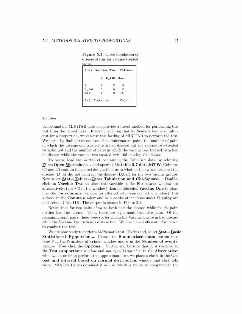
5.3. METHODS RELATED TO PROPORTIONS 47
Figure 5.1: Cross tabulation ofdisease status for vaccine treatedtwins.
Solution
Unfortunately, MINITAB does not provide a direct method for performing thistest from the paired data. However, recalling that McNemar’s test is simply atest for a proportion, we can use this facility of MINITAB to perform the test.We begin by finding the number of noninformative pairs, the number of pairsin which the vaccine one treated twin had disease but the vaccine two treatedtwin did not and the number of pairs in which the vaccine one treated twin hadno disease while the vaccine two treated twin did develop the disease.
To begin, load the worksheet containing the Table 5.7 data by selectingFile⇒Open Worksheet... and opening file table 5.7 data.MTW. ColumnsC1 and C2 contain the paired designations as to whether the twin contracted thedisease (D) or did not contract the disease (D bar) for the two vaccine groups.Now select Stat⇒Tables⇒Cross Tabulation and Chi-Square.... Double-click on Vaccine Two to place this variable in the For rows: window (oralternatively, type C2 in the window) then double-click Vaccine One to placeit in the For columns: window (or alternatively, type C1 in the window). Puta check in the Counts window and be sure the other items under Display areunchecked. Click OK. The output is shown in Figure 5.1.
Notice that for two pairs of twins both had the disease while for six pairsneither had the disease. Thus, there are eight noninformative pairs. Of theremaining eight pairs, there were six for whom the Vaccine One twin had diseasewhile the Vaccine Two twin was disease free. We now have sufficient informationto conduct the test.
We are now ready to perform McNemar’s test. To this end, select Stat⇒BasicStatistics⇒1 Proportion.... Choose the Summarized data: button thentype 8 in the Number of trials: window and 6 in the Number of events:window. Now click the Options... button and be sure that .5 is specified inthe Test proportion: window and not equal is specified in the Alternative:window. In order to perform the approximate test we place a check in the Usetest and interval based on normal distribution window and click OKtwice. MINITAB gives obtained Z as 1.41 which is the value computed in the

48 CHAPTER 5. PAIRED SAMPLES METHODS
text on page 176.The exact test is performed by following the above steps with the exception
that the Use test and interval based on normal distribution window isnot checked. In this case MINITAB gives the two-tailed p-value as .289 which isthe value calculated in conjunction with Example 5.11 on page 179 of the text.
Task 5.5
Use the Outcome variable in Table 5.14 to perform the exact test outlined inExample 5.13 on page 183.
Solution
Enter the Outcome variable, minus the noninformative observations, from Table5.14 into C1 of a new worksheet. Select Stat⇒Basic Statistics⇒1 Proportion....Select the Samples in columns: button and type C1 in the accompanyingwindow. Click the Options... button and enter .4 in the Test proportion:window. Select greater than in the Alternative: window and click OK twice.MINITAB gives the p-value for the test as 0.514 which is the value calculatedin the solution to Example 5.13.
Task 5.6
Construct the confidence intervals described in Example 5.15 on page 186.
Solution
Select Stat⇒Basic Statistics⇒1 Proportion.... Select the Summarizeddata button and enter 10 in the Number of trials: window and 4 in theNumber of events: window. Click on Options... and be sure that the Con-fidence level: window contains 95.0. Enter not equal in the Alternative:window and check the Use test and interval based on normal distribu-tion: box to obtain the approximate interval. Now click OK twice. MINITABdisplays the interval as (0.096364, 0.703636) which agrees with the calculationsobtained in the solution to Example 5.15.
Repeat the above steps with the Use test and interval based on nor-mal distribution: box unchecked. MINITAB gives the exact interval as(0.121552, 0.737622 which, except for rounding, again agrees with the calcu-lations provided in the solution to 5.15.
5.4 Methods Related to Paired Samples Risk
Ratios (page 190)
Task 5.7
Carry out the tasks outlined in Example 5.17 on page 191.

5.5. METHODS RELATED TO PAIRED SAMPLES ODDS RATIOS 49
Solution
MINITAB does not provide a direct means for calculating a paired samples riskratio. However, it can still be useful in such an endeavor in that it can be usedto form the data into a two by two table thereby facilitating the calculation.This can be particularly useful for large data sets.
For the problem at hand, generate the table shown in Figure 5.1 of this man-ual by following the steps given in Task 5.4. You can then use the informationgiven in this table to calculate the risk ratio via Equation 5.7 on page 191.
The test of significance conducted via Equation 5.4 was carried out in thesolution to Task 5.4. To obtain the result provided by Equation 5.5, simplysquare the result given by Equation 5.4.
Task 5.8
Use MINITAB to perform the equivalence test as outlined in Example 5.20 onpage 195.
Solution
Unfortunately, MINITAB does not provide a straightforward means for per-forming this test.
Task 5.9
Use MINITAB to form the confidence interval described in Example 5.22 onpage 197.
Solution
Unfortunately, MINITAB does not provide a straightforward means for con-structing this interval.
5.5 Methods Related to Paired Samples Odds
Ratios (page 199)
Task 5.10
Use MINITAB to test the hypothesis H0 : OR = 1 as described in Example5.24 on page 201.
Solution
Using the fact that a test of H0 : OR = 1 is equivalent to a test of H0 : π = .5, weconduct the test as follows. Select Stat⇒Basic Statistics⇒1 Proportion....Choose the Summarized data button and enter 30 in the Number of trials:window and 25 in the Number of events: window. The number of trials isspecified as 30 because after eliminating the noninformative pairs there are
50 CHAPTER 5. PAIRED SAMPLES METHODS
25 + 5 = 30 remaining pairs that do provide information. Of these, in twenty-five pairs, the member with cancer had been exposed while the pair memberwithout cancer was not exposed. We define this as the number of events.
Now click Options... and be sure that the Test proportion: is set to 0.5.Put a check in the Use test and interval based on normal distribution boxand click OK twice. MINITAB performs the test as a Z test while a chi-squarestatistic is reported in the text. By squaring obtained Z of 3.65 we obtain,except for rounding, the chi-square statistic of 13.33 reported in the text.
Task 5.11
Perform the exact two-tailed equivalence test described in Example 5.27 on page206.
Solution
Unfortunately, MINITAB does not provide a straightforward means of perform-ing this test. However, by using the relationship between the paired samplesodds ratio and proportions along with the so called shortcut method of perform-ing equivalence tests introduced on page 39, the task can be performed withouttoo much difficulty.
We begin by constructing a 90 (not 95) percent confidence interval for theestimation of π. To this end, select Stat⇒Basic Statistics⇒1 Proportion....Choose the Summarized data button and enter 15 in the Number of trials:window and 8 in the Number of events: window. Now click Options...and be sure that the Confidence level: is set to .90 and Alternative: isnot equal. Because we are conducting an exact test, be sure the Use testand interval based on normal distribution box is not checked. Click OKtwice. The confidence interval (0.299986, 0.756273) is displayed in the SessionWindow. Because this confidence interval is not contained in the equivalenceinterval EIL = .454 and EIU = .545, the equivalence null hypothesis is notrejected. This is the same conclusion reached in the Solution to Example 5.27.
Task 5.12
Construct the exact confidence interval described in Example 5.30 on page 211.
Solution
Unfortunately, MINITAB does not provide a straightforward means of con-structing this interval. However, by using the relationship between the pairedsamples odds ratio and proportions, we can construct the CI for the associatedproportion and then convert this interval for the estimation of π into an intervalfor estimating the paired samples OR.
To this end, select Stat⇒Basic Statistics⇒1 Proportion.... Choose theSummarized data button and enter 24 in the Number of trials: window and13 in the Number of events: window. Now click Options... and be sure thatthe Confidence level: is set to .95 and Alternative: is not equal. Because
5.5. METHODS RELATED TO PAIRED SAMPLES ODDS RATIOS 51
we are conducting an exact test, be sure the Use test and interval basedon normal distribution box is not checked. Click OK twice. The confidenceinterval (0.328208, 0.744470) is displayed in the Session Window. This is thesame interval reported as part of the solution to Example 5.30. In order toconvert this interval into an interval for the estimation of OR, you must applyEquation 5.17 (page 208) as is shown in the solution to Example 5.30.
52 CHAPTER 5. PAIRED SAMPLES METHODS
Exercises
5.1 Use MINITAB to perform the test of hypothesis outlined in Example 5.2on page 163.
5.2 Use MINITAB to perform the equivalence test outlined in Example 5.5 onpage 169.
5.3 Use the paired data in Table 5.2 to form a 95 percent confidence intervalfor the estimation of µ1 − µ2 where µ1 represents the mean for TreatmentOne and µ2 represents the mean for Treatment Two.
5.4 Use MINITAB to perform the test outlined in Example 5.12 on page 180.
5.5 Use the Outcome variable in Table 5.16 to perform the tests alluded to inExample 5.14 on page 185.
5.6 Use MINITAB to construct the confidence intervals discussed in Example5.16 on page 188.
5.7 Conduct the test outlined in Example 5.18.
5.8 Conduct the test of significance alluded to in Example 5.19 on page 192.
5.9 Use MINITAB to perform the exact two-tailed test of significance outlinedin Example 5.25 on page 202.
5.10 Use MINITAB to construct the approximate confidence interval discussedin Example 5.28 on page 208.
Chapter 6
Two Independent SamplesMethods
6.1 Introduction
In this chapter you will use MINITAB to perform tests of hypotheses and formconfidence intervals for various two (independent) sample methods. You willconduct independent samples t tests and tests for differences between propor-tions. You will also form confidence intervals for each of these statistics andperform equivalence tests.
6.2 Methods Related to Differences Between Means(page 215)
Task 6.1
Conduct the independent samples t test described in Example 6.1 on page 220.
Solution
Open the table 6.1 data.MTW worksheet. Select Stat⇒Basic Statistics⇒2-Sample t.... The 2-Sample t (Test and Confidence Interval) windowopens. Select the Samples in different columns button. Enter C1 in theFirst: window and C2 in the Second: window. Put a check in the Assumeequal variances box. Click the Options... button. Be sure that the Testdifference: window is set to 0.0 and the Alternative: window is set to notequal. Click OK twice. The result shown in Figure 6.1 appears in the SessionWindow.
Notice that obtained t is −0.81 which is the value calculated in the text. Theassociated p-value is 0.426 which results in failure to reject the null hypothesis
53

54 CHAPTER 6. TWO INDEPENDENT SAMPLES METHODS
Figure 6.1: MINITAB output for an independent samples ttest.
at the .05 level.
Task 6.2
Conduct the equivalence test described in Example 6.3 on page 225.
Solution
Open the table 6.1 data.MTW worksheet. Select Stat⇒Basic Statistics⇒2-Sample t.... The 2-Sample t (Test and Confidence Interval) windowopens. Select the Samples in different columns button. Enter C1 in theFirst: window and C2 in the Second: window. Put a check in the Assumeequal variances box. Click the Options... button. Set the Test difference:window to −5.0 and the Alternative: window to greater than. Click OK twice.The result appears in the Session Window. Notice that obtained t of 0.38 is thesame value calculated in the text. The associated p-value is 0.353 so that theequivalence null hypothesis is not rejected.
Task 6.3
Form the confidence interval described in Example 6.5 on page 228.
Solution
Open the table 6.1 data.MTW worksheet. Select Stat⇒Basic Statistics⇒2-Sample t.... The 2-Sample t (Test and Confidence Interval) windowopens. Select the Samples in different columns button. Enter C1 in theFirst: window and C2 in the Second: window. Put a check in the Assumeequal variances box. Click the Options... button. Be sure the Confidencelevel: is set to 95.0 and the Alternative: is set to not equal. Click OK twice.MINITAB prints the following in the Session Window.
“95% CI for difference: (-12.02002, 5.22002)”
This is the interval calculated in the text.

6.3. METHODS RELATED TO PROPORTIONS 55
6.3 Methods Related to Proportions (page 230)
Task 6.4
Perform the two sample test for a difference between proportions addressed inExample 6.7 on page 233.
Solution
Select Stat⇒Basic Statistics⇒2 Proportions.... In the 2 Proportions(Test and Confidence Interval) window, choose the Summarized databutton. In the First: window enter 314 for Trials: and 23 for Events:. Inthe Second: window enter 316 for Trials: and 39 for Events:. Now click theOptions... button. Be sure that Test difference: is set to 0.0, Alternative:is not equal and the Use pooled estimate of p for test box is not checked.Now click OK twice. MINITAB reports obtained Z as −2.12, which is the resultreported in the text, with an associated p-value of 0.034. This value would beappropriate for a two-tailed test. For the one-tailed test addressed here wecalculate .034/2 = .017 which causes the null hypothesis to be rejected.
Task 6.5
Perform the two-tailed equivalence test described in Example 6.9 on page 235.
Solution
For Test One, select Stat⇒Basic Statistics⇒2 Proportions.... In the 2Proportions (Test and Confidence Interval) window, choose the Sum-marized data button. In the First: window enter 100 for Trials: and 7 forEvents:. In the Second: window enter 100 for Trials: and 6 for Events:.Now click the Options... button. Set Test difference: to 0.04, Alternative:to less than and be sure the Use pooled estimate of p for test box is notchecked. Now click OK twice. MINITAB reports obtained Z as −.86, which isthe result reported in the text, with an associated p-value of 0.195.
For Test Two, follow the same steps as for Test One with the exception thatTest difference: is set to -.04 and Alternative: to greater than. MINITABgives obtained Z as 1.43, which is the value calculated in the text, with anassociated p-value of 0.076. Thus, the equivalence null hypothesis is not rejected.
Task 6.6
Construct the confidence interval described in Example 6.11 on page 236.
Solution
Select Stat⇒Basic Statistics⇒2 Proportions.... In the 2 Proportions(Test and Confidence Interval) window, choose the Summarized databutton. In the First: window enter 299 for Trials: and 106 for Events:.
56 CHAPTER 6. TWO INDEPENDENT SAMPLES METHODS
In the Second: window enter 313 for Trials: and 66 for Events:. Nowclick the Options... button. Be sure that Confidence level: is set to 95.0,Alternative: is not equal and the Use pooled estimate of p for test boxis not checked. Now click OK twice. MINITAB reports the confidence intervalas (0.0730676, 0.214237). Notice that these values differ slightly from thosecalculated in the text. This is because the methods used by MINITAB and thetext for constructing such intervals differ slightly. The method used in the textis slightly more conservative and, in the opinion of the authors, is preferable.
6.4 Methods Related to Independent SamplesRisk Ratios (page 238)
Unfortunately, MINITAB does not implement the methods discussed in the textfor dealing with independent samples risk ratios.
6.5 Methods Related to Independent Samples
Odds Ratios (page 247)
Unfortunately, MINITAB does not implement the methods discussed in the textfor dealing with independent samples odds ratios.

Exercises 57
Exercises
6.1 The MINITAB output associated with Task 6.1 contains the statement“Both use Pooled StDev = 11.5245.” How does the value 11.5245 relateto the calculations carried out in the text in conjunction with Example 6.1?
6.2 Use MINITAB to conduct the test of hypothesis described in Example 6.2.
6.3 Perform the equivalence test described in Example 6.4 on page 226.
6.4 Find the confidence interval discussed in Example 6.6 on page 229.
6.5 Perform the test described in Example 6.8 on page 233.
6.6 Perform the equivalence test outlined in Example 6.10 on page 235.
6.7 Construct the one-sided confidence interval described in Example 6.12 onpage 237.

58 CHAPTER 6. TWO INDEPENDENT SAMPLES METHODS

Chapter 7
Multi-Sample Methods
7.1 Introduction
In this chapter you will use MINITAB to perform a One-Way ANOVA, a 2 byk chi-square test and Tukey’s HSD test.
7.2 The One-Way Analysis of Variance (ANOVA)
F Test (page 264)
Task 7.1
Use the data in Table 7.1 to compute MSw, MSb, obtained F and to producean ANOVA table.
Solution
Load the table 7.1b data.MTW worksheet. Notice that C2 contains theweights of the 15 subjects while C1 contains an indicator (1, 2, or 3) as towhich group the weight represents. Select Stat⇒ANOVA⇒One-Way.... TheOne-Way Analysis of Variance window opens. Type C2 in the Response:window and C1 in the Factor: window. Click OK. The relevant portion of theMINITAB output is shown in Figure 7.1.
In the ANOVA table provided by MINITAB, between groups elements arelabeled “Factor” while within group elements are labeled “Error.” From thetable we see that MSw and MSb are given as 625 and 935 respectively. Exceptfor rounding, these are the values calculated in the text. Obtained F is givenas 1.50 which is the value given in the text. The associated p-value is .263.
59

60 CHAPTER 7. MULTI-SAMPLE METHODS
Figure 7.1: MINITAB rendering of ANOVAtable for data in text Table 7.1.
Figure 7.2: Nutritional data ar-ranged for chi-square analysis.
7.3 The 2 By k Chi-Square Test (page 276)
Task 7.2
Perform the chi-square test outlined in Example 7.6 on page 280.
Solution
Open a new worksheet. Label C1 “Instruction” and C2 “No Instruction.” Nowenter the number of Low Birth Weight babies for the Instruction group in R1C1and the number of No Low Birth Weight babies in R2C1. Enter the correspond-ing values for the No Instruction group in R1C2 and R2C2. Your worksheetshould appear as in Figure 7.2.
To perform the analysis, select Stat⇒Tables⇒Chi-Square Test (Tablein Worksheet).... Enter C1 C2 in the Columns containing the table:window and click OK. The output is shown in Figure 7.3. Notice that in addi-tion to obtained chi-square with it’s associated p-value, the output also showsthe observed and expected frequencies for each cell along with the contributionmade by that cell to the overall chi-square value.1
1That is, the values summed in the calculation of obtained chi-square.

7.4. MULTIPLE COMPARISON PROCEDURES 61
Figure 7.3: Chi-square analysis of nutritional data.
7.4 Multiple Comparison Procedures (page 282)
Task 7.3
Perform the Tukey’s HSD tests outlined in Example 7.9 on page 289.
Solution
Load the table 7.1b data.MTW worksheet. Notice that C2 contains theweights of the 15 subjects while C1 contains an indicator (1, 2, or 3) as towhich group the weight represents. Select Stat⇒ANOVA⇒One-Way.... TheOne-Way Analysis of Variance window opens. Type C2 in the Response:window and C1 in the Factor: window. Click the Comparisons... button.Put a check in the Tukey’s, family error rate: box and enter .05 in theaccompanying window. Click OK twice. In addition to the ANOVA table, theoutput shown in Figure 7.4 appears in the Session Window.
Notice that comparisons are made in terms of confidence intervals ratherthan hypothesis tests as is done in the text. Thus, the comparison µ2 − µ1
2
is represented by the interval L = −34.35, U = 49.95. Because zero is in theinterval, the null hypothesis is not rejected. This is true of the remaining com-parisons as well so that the conclusions provided by MINITAB are the same asthose reached in the text.
2This comparison is represented as µ1 − µ2 in the text.
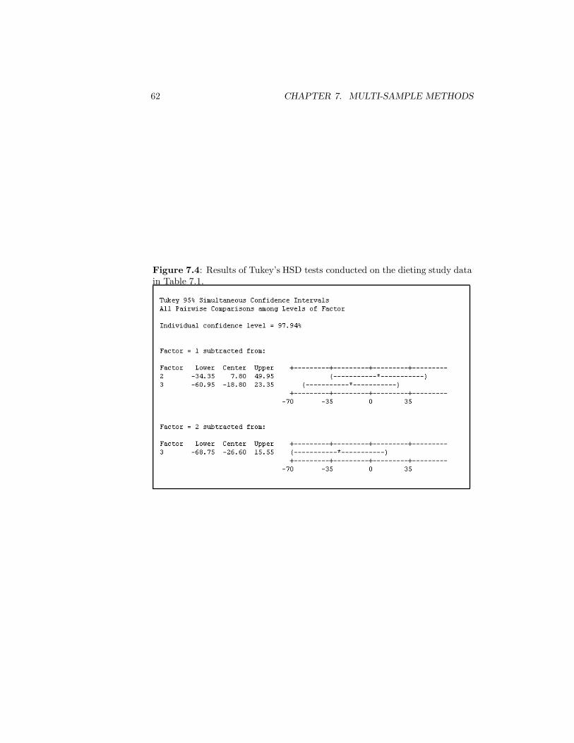
62 CHAPTER 7. MULTI-SAMPLE METHODS
Figure 7.4: Results of Tukey’s HSD tests conducted on the dieting study datain Table 7.1.

Exercises 63
Exercises
7.1 Carry out the ANOVA analysis outlined in Example 7.3 on page 269.
7.2 Carry out the ANOVA analysis outlined in Example 7.4 on page 271.
7.3 Perform the chi-square analysis outlined in Example 7.5 on page 279.
7.4 Perform the multiple comparison tests outlined in Example 7.10 on page290.

64 CHAPTER 7. MULTI-SAMPLE METHODS

Chapter 8
The Assessment ofRelationships
8.1 Introduction
In this chapter you will use MINITAB to calculate the Pearson product-momentcorrelation coefficient and to test the hypothesis H0 : ρ = 0. Additionally, youwill conduct the chi-square test for independence.
8.2 The Pearson Product-Moment CorrelationCoefficient (page 295)
Task 8.1
Calculate the Pearson product-moment correlation coefficient for the data inTable 8.1 on page 297. Perform a two-tailed test of the hypothesis H0 : ρ = 0at the .05 level.
Solution
Load the table 8.1 data.MTW worksheet. Select Stat⇒Basic Statistics⇒Correlation....Enter x and y in the Variables: window and be sure the Display p-valuesbox is checked. Click OK. MINITAB displays the correlation as 0.964 which isthe value calculated in the text. The associated p-value of 0.000 results in rejectof the null hypothesis H0 : ρ = 0.
65

66 CHAPTER 8. THE ASSESSMENT OF RELATIONSHIPS
Figure 8.1: Chi-square analysis of data de-scribed in Example 8.7.
8.3 The Chi-Square Test For Independence (page312)
Task 8.2
Perform the chi-square test described in Example 8.7 on page 314.
Solution
Enter the observed frequencies into a new worksheet as shown in manual Fig-ure 8.1. Then select Stat⇒Tables⇒Chi-Square Test (Table in Work-sheet).... Enter C1 C2 C3 in the Columns containing the table: windowand click OK. The observed and expected frequencies for each cell of the tableare printed along with the contribution made by each cell to the overall chi-square statistic. Obtained chi-square of 206.811 is reported with 4 degrees offreedom and an associated p-value 0.000.

Exercises 67
Exercises
8.1 Calculate the correlation coefficient discussed in Example 8.2 on page 298.

68 CHAPTER 8. THE ASSESSMENT OF RELATIONSHIPS

Chapter 9
Linear Regression
9.1 Introduction
In this chapter, you will use MINITAB to construct simple and multiple regres-sion models, generate R2 values and conduct tests of significance.
9.2 Simple Linear Regression (page 320)
Task 9.1
Construct the simple linear regression model alluded to in Example 9.1 on page321.
Solution
Open the table 8.2 data worksheet. Select Stat⇒Regression⇒Regression....In the Regression window, type C2 in the Response: window and C1 in thepredictors: window. Click Options... and be sure there is a check in the Fitintercept box. Click OK twice. MINITAB gives the regression equation asy = 0.874 + 0.706 x which is the result given in the text.
Task 9.2
Find SSreg , SSres, and R2 for the data in Table 9.1 on page 323.
Solution
Open the table 9.1 data worksheet. Select Stat⇒Regression⇒Regression....In the Regression window, type C1 in the Response: window and C2 in thepredictors: window. Click Options... and be sure there is a check in theFit intercept box. Click OK twice. MINITAB gives the Regression sum ofsquares (SSreg ) as 107.44 and the Residual Error sum of squares (SSres) as
69
70 CHAPTER 9. LINEAR REGRESSION
8.29 which agrees with the values calculated in the text. R2 is given as R-Sq =92.8% which is the value calculated in the solution to Example 9.2 on page 324.
Task 9.3
Test the null hypothesis R2 = 0 for a model used to predict y from x for thedata in Table 9.1 on page 323.
Solution
Using the output from the solution to Task 9.2, we see that obtained F isreported as 168.49 with an associated p-value of 0.000. The value of 168.49reported by MINITAB differs slightly from the value of 167.56 calculated in thetext. This small difference appears to be the result of differences in rounding.
9.3 Multiple Linear Regression (page 329)
Task 9.4
Use the data in Table 9.2 on page 330 to construct a two predictor model withx1 and x2 being used to predict y.
Solution
Open the table 9.2 data worksheet. Select Stat⇒Regression⇒Regression....In the Regression window, type C1 in the Response: window and C2 C3 inthe predictors: window. Click Options... and be sure there is a check inthe Fit intercept box. Click OK twice. MINITAB gives the regression modelas y = 2.69 + 0.404 x1 + 1.00 x2 which agrees with the results calculated in thetext.
Task 9.5
Test the null hypothesis H0 : β1 = β2 = 0 for the model you constructed inTask 9.4.
Solution
From the output for the solution to Task 9.4, we note that obtained F forthe regression model is 4.73 which is the value calculated in the text. Theassociated p-value is 0.031 which results in rejection of the null hypothesis fora test conducted at α = .05. This is the same conclusion reached in the text.
Task 9.6
Use the data in Table 9.2 on page 330 to determine whether adding x2 to amodel that contains x1 adds significantly to R2.

9.3. MULTIPLE LINEAR REGRESSION 71
Figure 9.1: Sequential General Linear Model analysis ofTable 9.2 data.
Solution
This problem can be approached in a number of different ways. For example,we could use MINITAB to find R2
y.1 and R2y.12 then use a calculator to apply
Equation 9.24. We will use a more direct, if somewhat less obvious, approach.Select Stat⇒ANOVA⇒General Linear Model.... The General Linear
Model screen opens. Type y in the Responses: window and x1 x2 in theModel: window. To this point we have set up a model in which y is thedependent variable with x1 and x2 being predictors. Now click on Covariates...and enter x1 x2 in the Covariates: window. Among other things, this lastaction cause MINITAB to treat x1 and x2 as continuous variables rather thantransforming them as might be done in other forms of analysis. Click OK. Nowclick Options.... In the Sum of Squares: column, darken the Sequential(Type I) button. Click OK twice. The relevant portion of the output is shownin manual Figure 9.1. This output will require some explanation.
Of interest for the problem at hand are the headings labeled “Seq SS” (Se-quential Sum of Squares), “F” (obtained F), and “P” (p-value). The Seq SSvalues represent the increment in SSreg that occurs as each variable is added tothe model.1 Thus, with only x1 in the model, SSreg was 150.83. Adding x2 tothe model increased this value by 90.78. It will be instructive to convert thesevalues into expressions of R2. This can be done by dividing each value by SSy
which is labeled in the printout as “Total.” For x1 we have
R2 =150.83548.40
= .2750
which is equal to R2y.1. Of more interest is the R2 value obtained from x2 which
is
R2 =90.78548.40
= .1655
which is equal to R2y.12 − R2
y.1. The values of F reported in the output are thevalues of obtained F for a test of significance on each of the incremental sums ofsquares. It follows that obtained F of 3.55 is obtained F for a test conducted on
1The order in which variables are added to the model is determined by the order in whichthey are listed in the Model: window.

72 CHAPTER 9. LINEAR REGRESSION
R2y.12 − R2
y.1. Indeed, this is the value calculated on page 337 of the text. Theassociated p-value of 0.084 means that we would fail to reject the null hypothesisR2
y.12 −R2y.1 = 0 at the .05 level. This is the conclusion reached on page 337 of
the text. Therefore, we are unable to demonstrate that adding x2 to a modelthat contains x1 adds to R2.
To further elucidate, suppose we were working with four predictors, x1,x2, x3 and x4 and had entered them in that order in the Model: box. Theobtained F and associated p-values for each predictor would represent tests ofthe following null hypotheses.
Source Hypothesis
x1 R2y.1 = 0
x2 R2y.12 − R2
y.1 = 0
x3 R2y.123 − R2
y.12 = 0
x4 R2y.1234 − R2
y.123 = 0
Exercises 73
Exercises
9.1 Find the regression equation for predicting y from x for the data in Table9.1 on page 323.
9.2 Use MINITAB to construct the model described in Exercise 9.7 on page341 of the text.
9.3 Test the null hypothesis H0 : R2 = 0 for the model you constructed inExercise 9.2.
9.4 Use the data in Table 9.2 on page 330 to determine whether adding x1 to amodel that contains x2 adds significantly to R2.

74 CHAPTER 9. LINEAR REGRESSION
Chapter 10
Methods Based on thePermutation Principle
10.1 Introduction
In this chapter you will use MINITAB to perform Wilcoxon’s signed-ranks test,Wilcoxon’s rank-sum (Mann-Whitney) test, the Kruskal-Wallis test and Fisher’sexact test.
10.3 Applications (page 348)
Task 10.1
Perform the Wilcoxon’s signed-ranks test described in Example 10.15 on page369.
Solution
Open the table 10.7 data.MTW worksheet. Notice that this file containsdifference scores rather than the pre- and post-treatment values. Select Stat⇒Nonparametrics⇒1-Sample Wilcoxon.... Type C1 or d in the Variables:window. Darken the Test median: button and type 0.0 in the accompanyingwindow if necessary. Be sure the Alternative: window is set to not equal.Click OK.
MINITAB reports the test p-value as 0.262 which results in failure to rejectthe null hypothesis at α = .05. This is the same conclusion reached in the text.It should be noted, however, that p-values reported by MINITAB for Wilcoxon’ssigned-ranks are approximations rather than exact values.
75
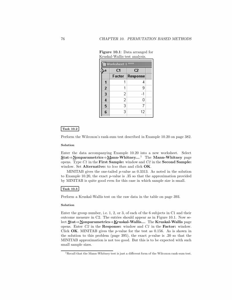
76 CHAPTER 10. PERMUTATION BASED METHODS
Figure 10.1: Data arranged forKruskal-Wallis test analysis.
Task 10.2
Perform the Wilcoxon’s rank-sum test described in Example 10.20 on page 382.
Solution
Enter the data accompanying Example 10.20 into a new worksheet. SelectStat⇒Nonparametrics⇒Mann-Whitney....1 The Mann-Whitney pageopens. Type C1 in the First Sample: window and C2 in the Second Sample:window. Set Alternative: to less than and click OK.
MINITAB gives the one-tailed p-value as 0.3313. As noted in the solutionto Example 10.20, the exact p-value is .35 so that the approximation providedby MINITAB is quite good even for this case in which sample size is small.
Task 10.3
Perform a Kruskal-Wallis test on the raw data in the table on page 393.
Solution
Enter the group number, i.e. 1, 2, or 3, of each of the 6 subjects in C1 and theiroutcome measure in C2. The entries should appear as in Figure 10.1. Now se-lect Stat⇒Nonparametrics⇒Kruskal-Wallis.... The Kruskal-Wallis pageopens. Enter C2 in the Response: window and C1 in the Factor: window.Click OK. MINITAB gives the p-value for the test as 0.156. As is shown inthe solution to this problem (page 395), the exact p-value is .20 so that theMINITAB approximation is not too good. But this is to be expected with suchsmall sample sizes.
1Recall that the Mann-Whitney test is just a different form of the Wilcoxon rank-sum test.
10.3. APPLICATIONS 77
Task 10.4
Perform a two-tailed Fisher’s exact test on the data in Table 10.23 on page 405.
Solution
Open the table 10.23 data.MTW worksheet. Notice that C1 contains rownumbers and C2 the column numbers of the cells that makeup Table 10.23.Taken together, these columns uniquely identify each cell of the table. ColumnC3 provides the frequency in each of the four cells.
Select Stat⇒Tables⇒Cross Tabulation and Chi-Square.... The CrossTabulation and Chi-Square page opens. Type C1 in the For rows: window,C2 in the For columns: window and C3 in the Frequencies are in: window.Now click Other Stats... and place a check in the Fisher’s exact test for2x2 tables box. Click OK twice.
MINITAB gives the p-value for the test as 0.0889111 which is the valuecalculated for a two-tailed test in the solution to Example 10.30 on page 405.Notice that MINITAB did not provide the option of performing a one-tailedtest.

78 CHAPTER 10. PERMUTATION BASED METHODS
Exercises
10.1 Conduct the test described in Example 10.16 on page 371.
10.2 Perform the test alluded to in Example 10.21 on page 383.
10.3 Conduct the test described in Example 10.22 on page 385.
10.4 Conduct the Kruskal-Wallis test described in Example 10.27 on page 395.
10.5 Conduct the test described in Example 10.31 on page 407.

Appendix A
Table Relating Text Itemsto Tasks
This table relates various portions of the text to specific tasks and the task pagenumber.
Text Task Page
Table 2.2 2.1 11Table 2.3* 2.2 13Table 2.4 2.3 13Figure 2.1 2.4 15Table 2.3* 2.5 17Figure 2.4 2.6 18Figure 2.6 2.7 19Example 2.4 2.9 24Example 2.7 2.10 25Table 2.6 2.11 26Example 2.17 2.12 28Example 2.21 2.13 28Example 2.23 2.14 28Example 2.24 2.15 29Table 3.1 3.1 31Example 3.9 3.2 31Table 4.1 4.1 35Example 4.7 4.2 36Example 4.9 4.3 36Example 4.12 4.4 37
79

80 APPENDIX A. TABLE RELATING TEXT ITEMS TO TASKS
Text Task Page
Example 4.14 4.5 38page 108 4.6 38Example 4.19 4.7 39Example 4.25 4.8 39Example 4.26 4.9 40Example 4.32 4.10 41Example 4.34 4.11 41Example 4.36 4.12 42Example 4.37 4.13 42Example 4.41 4.14 43Example 4.42 4.15 43Example 5.1 5.1 45Example 5.4 5.2 46Table 5.1 5.3 46Table 5.7 5.4 46Example 5.13 5.5 48Example 5.15 5.6 48Example 5.17 5.7 48Example 5.20 5.8 49Example 5.22 5.9 49Example 5.24 5.10 49Example 5.27 5.11 50Example 5.30 5.12 50Example 6.1 6.1 53Example 6.3 6.2 54Example .6.5 6.3 54Example 6.7 6.4 55Example 6.9 6.5 55Example 6.11 6.6 55Table 7.1 7.1 59Example 7.6 7.2 60Example 7.9 7.3 61Table 8.1 8.1 65Example 8.7 8.2 66Example 9.1 9.1 69Table 9.1* 9.2 69Table 9.1* 9.3 70Table 9.2* 9.4 70Table 9.2* 9.5 70
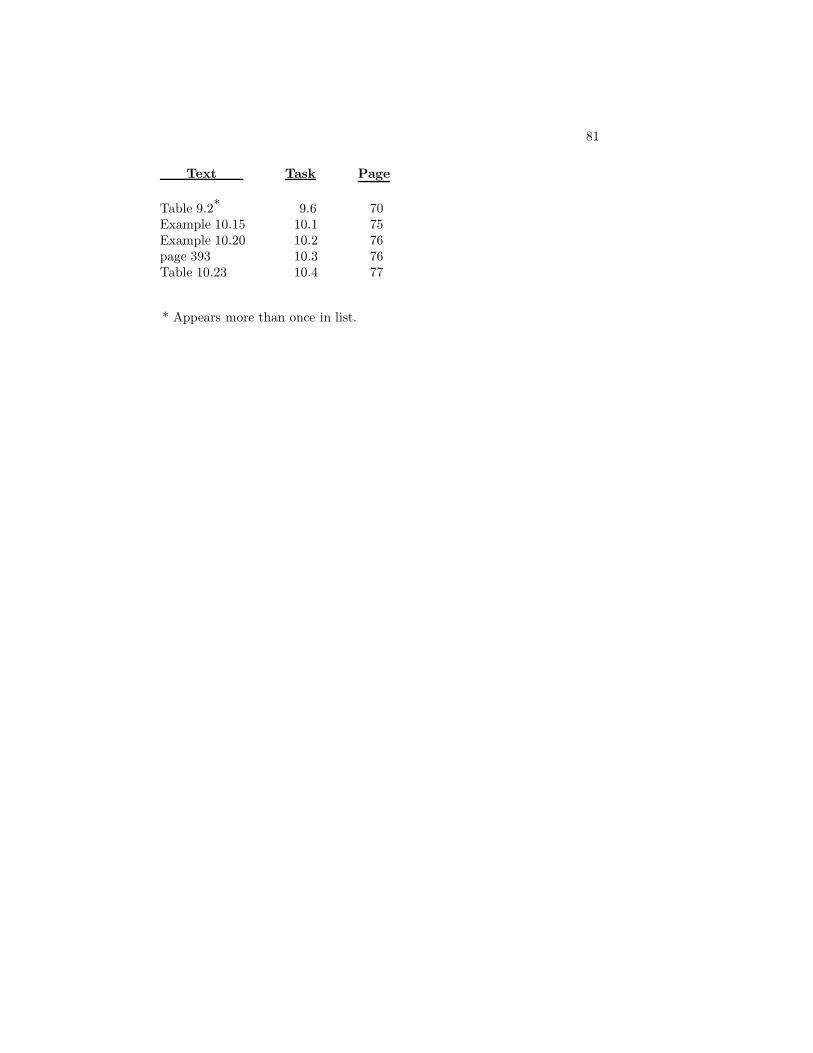
81
Text Task Page
Table 9.2* 9.6 70Example 10.15 10.1 75Example 10.20 10.2 76page 393 10.3 76Table 10.23 10.4 77
* Appears more than once in list.