minimum coverage design in wireless surveillance networks

International Journal of Emerging Trends & Technology in Computer Science (IJETTCS) Web Site: www.ijettcs.org Email: [email protected]

Volume 3, Issue 5, September-October 2014 ISSN 2278-6856

Volume 3, Issue 5, September-October 2014 Page 22

Abstract This paper presents a new application-oriented review on analysis and improvement of the primary QoS indicators of the Wireless Sensor Network (WSN) applications described in the context and scope of the newly introduced concept of minimum coverage. Although crucial and design-critical, especially in the quasi-randomly deployed networks, so far, the problem of minimum coverage is mainly treated regarding a specific implementation and/or in the process of the (energy) optimization, implicitly encapsulated in one of the general definitions of coverage. Based on the existing work related to the particular implementations, the paper provides a more generic design-based and application-centered approach to the evaluation and improvement of the minimum coverage for a wide range of applications. Furthermore, and in contrast to the previous surveys on this topic, the critical variables that influence the minimum coverage are clustered and sublimated into categories that are further sub-clustered, described, and compared regarding the application-specific requirements. A newly introduced cross-cluster design-oriented scheme that takes the application requirement as an input and sequentially involves various variables towards the process of evaluation and/or improvement of the minimum coverage, aims also to serve as a literature-based systemized guideline on establishing the working point of the WSN application. Keywords: Coverage, Detectability, Deployment, Modeling, Sensing Models, Wireless Sensor Networks.

1. INTRODUCTION Modern surveillance networks are consisted of various types of technologies, ranging from wireless long-range communications and ordinary computer networks to the networks of small sensor nodes with short-range wireless communication capability. At the lowest tier of their architecture, in most of the cases, these networks contain the systems for data acquisition that directly interface the environment. Although there are other similar types of sensor systems and networks (such as ad-hoc networks, wired sensor systems, etc.) that can also be used as a part of the surveillance networks, systems that pose sensing, computing and networking capabilities are mainly classified as WSNs. The WSN is the most critical part of the wireless surveillance system architecture that consists of small microelectronic devices – nodes equipped with sensing, processing and communication elements. The nodes are, however, very limited regarding all the computational and communication resources and capabilities, mainly because of their power autonomy and small physical dimensions. Moreover, and most importantly regarding the context of this paper, sometimes a network needs to be deployed quasi-randomly in an unfriendly terrain such as in inaccessible regions (in

military applications) or the forests. In these situations, covering the area of interest with the small quasi-randomly deployed autonomous nodes that automatically start sensing the phenomenon and communicating the sensed information to the outer network immediately after the deployment, is not always an easy task. Before delving into the other quality measures, the coverage and connectivity are the primary Quality of Service (QoS) issues that need to be addressed in a WSN-based application. They express the quality at which the WSN can meet the main application requirements: to cover the whole area of interest and to transfer data between two points of interest, respectively. Although, the term of coverage is dually used in literature: in the context of the region that is covered by the network’s sensing field and in the context of the region that offer the node’s connectivity in the network; in this paper, by term coverage, we refer to the sensing coverage. It can be defined as the ability of the network to efficiently cover the whole area of interest by the sensing fields of its connected nodes. The WSN’s efficiency can be measured and optimized in many ways, mainly regarding the energy consumption. But the optimization philosophy in most of the protocols and algorithms rely on the assumption that the appropriate communication between nodes is physically achievable and that the network already has the ability to sense the phenomenon of interest. This means that, along with the minimum connectivity, the minimum coverage is here implied. But, the minimum coverage and connectivity are sometimes hardly achievable and depend on many factors such as: the electro-mechanic characteristics of the sensor nodes, the primary resources (number of nodes and the sensing range), the deployment manner, the area of interest, the deployment environment etc. Consequently, the minimum coverage mathematically presents one of the two required conditions for achieving all the other QoS requirements. Although as important as sensing coverage, the minimum connectivity is not explicitly covered in this paper. As noted in [1], however, in some implementations, the minimum connectivity can be implied by the sensing coverage. The efficiency of the network coverage can be qualified in two directions: a) in terms of minimizing the required number of nodes to cover the whole area of interest given the (variable) sensing radius, and, b) in terms of energy efficiency or reliability of the specific coverage protocol, i.e., the optimization. The first qualification is important in two aspects: a) in the direction of the cost minimization, and b) in the sense of analysis and improvement of the (probabilistic) coverage in randomly deployed networks. In order to address these issues, we introduce a new concept - the minimum

Minimum Coverage Design in Wireless Surveillance Networks

Zhilbert Tafa Department of Computer Science and Engineering

University for Business and Technology, Prishtina, Kosova



Volume 3, Issue 5, September-October 2014 3

coverage, a metrics that covers both possibilities and presents the ability of the network to cover the whole area of interest by minimum number of sensor nodes. After achieving the minimum coverage, the most important questions are related to the energy efficiency which is strongly related to the issues of the network lifetime and the reliability. In WSN, the energy efficiency can be addressed in the following ways [2]:

1) By scheduling the wireless nodes to alternate between active and sleep mode,

2) By implementing the energy efficient protocols. 3) By adjusting the transmission range of the nodes. 4) By reducing the amount of data transmitted.

Except for the solutions 3) and 4) which depend on the hardware capabilities and the aggregation algorithms, these issues are usually addressed by increasing the network density, i.e., by providing the redundancy in the network where a specific point of the area of interest is covered by at least k nodes. This type of approach is also used in improving the network reliability. It is defined as k-coverage and it belongs to the process of optimization, as presented in Section 4. Actually, most of the literature treats the coverage issue from the optimization point of view. These algorithms are either centralized or distributed [2-13]. Thorough surveys on energy-aware coverage algorithms are given in [14] and [15]. Interestingly, all the papers that treat the coverage problem from the optimization point of view, consider the minimum coverage (as defined above) as priory established. There are only a very few attempts in literature where the minimum coverage is implicitly treated, but only in context of a specific problem or the application. A survey on coverage strategies in WSNs is given in [16]. In [17], some of the most important aspects regarding minimum network coverage for the deterministic network deployment are given. In contrast to the mentioned references, the newly introduced concept of minimum coverage integrates the best practices in modeling, analyzing, and improvement of the fundamental network ability to sense the phenomenon of interest in most typical implementations. Factors that influence the minimum coverage evaluation and improvement are grouped as depicted in Fig. 1.

Figure 1: Parameters that directly influence or are related to the minimum coverage problem.

Minimum coverage is calculated and/or improved in context of a specific coverage type. It depends on the shape and the size of the sensor’s sensing field (i.e., the sensing model of a node), the deployment model, the network

density, etc. In accordance to this model, the paper is organized as follows. After defining the new concept and its scope, the existing sensing and energy models are surveyed and discussed in Section 2. This section also contains the original classification of the sensing models and covers the impact of the energy models on minimum coverage. While relying on the most typical application scenarios, priory presented in Section3, the calculation and the improvement of the minimum coverage is presented in the context of various areas of interest defined by the design requirements in Section 4. The analysis constitutes the specifications for the minimum coverage requirements, approaches and improvements for all of the typical implementations. Before delving into this process, the original algorithmic representation aims to highlight the parameter dependencies and decision steps towards the minimum coverage analysis and improvement. In Section 4, for each of the deployment settings and each of the typical measures of the area of interest, the most significant available approaches on achieving and improving the minimum coverage are presented and discussed. Section 4 is divided into two subsections that separately treat the problem of minimum coverage in the context of deterministic and random deployments. Moreover, the second subsection divides the problem into two more sub-problems: when the network consists of only static nodes or when it incorporates some kind of nodes’ mobility. Finally, section V discuss the most important moments of the paper and concludes the paper.

2. SENSING AND ENERGY MODELING Sensor nodes sense the physical phenomenon in their vicinity. This area around a sensor is called the sensing field of a sensor. The coverage is calculated based on the sensing fields of all of the deployed sensors. It can be evaluated (and improved) if the shape of the sensing field is priory known or estimated. In this direction, many 3-D and 2-D models are used in literature. The 3-D representation of the sensing field is used in applications deployed in atmosphere, mapping of the topographical properties, underwater, and space. In 3-D representation, the sensing field is considered to be a sphere centered at the sensor node. A distributed algorithm that uses the 3-D representation for determining if the k-coverage is achieved is presented in [18]. Coverage in context of 3-D space is also analyzed in [17]. However, most of the papers analyze the 2-D case of coverage by modeling the sensing area around the sensor nodes in 2-D space. Although this area is never of regular shape such as disc, in most of the cases it is modeled by a circular region characterized by the sensing radius Rs. This disk model, also called Boolean or binary sensing model [19-21], is especially useful when some general conclusions about the behavior of the coverage are more important than the exact calculation of the network coverage. The model ignores the environmental conditions, i.e., obstacles and other propagation characteristics. Here, a sensor detects the event or target with the probability P=1 if the target is at




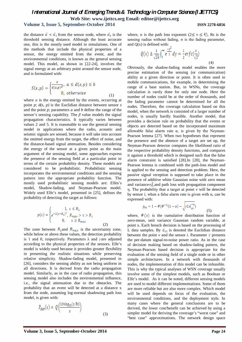
the distance from the sensor node, where is the threshold sensing distance. Although the least accurate one, this is the mostly used model in simulations. One of the methods that include the physical properties of a sensor, the energy emitted from the event, and the environmental conditions, is known as the general sensing model. This model, as shown in [22-24], involves the signal energy at an arbitrary point around the sensor node, and is formulated with:

(1) where α is the energy emitted by the events, occurring at point p; d(s, p) is the Euclidian distance between sensor s and the point p; parameters a and b define the range of the sensor’s sensing capability. The β value models the signal propagation characteristics. It typically varies between values 2 and 5. It is reasonable to use the general sensing model in applications where the radio, acoustic and seismic signals are sensed, because it will take into account the emitted energy from the target, the effect of noise, and the distance-based signal attenuation. Besides considering the energy of the sensor at a given point as the main argument of the sensing model, some approaches express the presence of the sensing field at a particular point in terms of the certain probability density. These models are considered to be probabilistic. Probabilistic sensing incorporates the environmental conditions and the sensing pattern into the appropriate probability function. The mostly used probabilistic sensing models are: Elfes’s model, Shadow-fading, and Neyman-Pearson model. Widely used Elfe’s model, presented in [25], defines the probability of detecting the target as follows:

(2) The zone between and is the uncertainty zone, while below or above these values, the detection probability is 1 and 0, respectively. Parameters λ and are adjusted according to the physical properties of the sensors. Elfe’s model is widely used because it provides greater flexibility in presenting the realistic situations while preserving relative simplicity. Shadow-fading model, presented in [26], considers the sensing ability as not being uniform in all directions. It is derived from the radio propagation model. Similarly, as in the case of radio propagation, this sensing model also includes the environmental influence, i.e., the signal attenuation due to the obstacles. The probability that an event will be detected at a distance x from the node, assuming log-normal shadowing path loss model, is given with:

(3)

where, n is the path loss exponent (2 , Rs is the sensing radius without fading, σ is the fading parameter, and Q(x) is defined with:

(4) Obviously, the shadow-fading model enables the more precise estimation of the sensing (or communication) ability at a given direction or point. It is often used in mobile communications, for example, in determining the range of a base station. But, in WSNs, the coverage calculation is rarely done for only one node. Here the number of nodes could be at the order of thousands, and the fading parameter cannot be determined for all the nodes. Therefore, the coverage calculation based on this model, when the network is consisted of a larger number of nodes, is usually hardly feasible. Another model, that provides a decision rule on probability that the events or objects are detected based on the incorporated maximum allowable false alarm rate α, is given by the Neyman-Pearson lemma [27]. When two hypotheses that represent the presence and the absence of a target are set up, the Neyman-Pearson detector computes the likelihood ratio of the respective probability density functions, and compares it against a threshold which is designed such that the false alarm constraint is satisfied [28].In [28], the Neyman-Pearson lemma is combined with the path-loss model and is applied to the sensing and detection problem. Here, the passive signal reception is supposed to take place in the presence of additive white Gaussian noise with zero mean and variance ,and path loss with propagation component η. The probability that a target at point v will be detected by sensor i, when a false alarm rate is given with α, can be expressed with:

(5) where, is the cumulative distribution function of zero-mean, unit variance Gaussian random variable, at point x. Each breach decision is based on the processing of L data samples. By is denoted the Euclidian distance between the point v and the sensor i. Parameter presents the per-datum signal-to-noise power ratio. As in the case of decision making based on shadow-fading pattern, the Neyman-Pearson based decision is appropriate for the evaluation of the sensing field of a single node or in other simple architectures. In a network with thousands of nodes, the implementation of this model can be infeasible. This is why the typical analyses of WSN coverage usually involve some of the simplest models, such as Boolean or Elfe’s model. As it can be noted, different sensing models are used to model different implementations. Some of them are more reliable but are also more complex. Which model will be used depends on focus of the evaluation, the environmental conditions, and the deployment style. In many cases where the general conclusions are to be derived, the lower cost/benefit can be achieved by using a simpler model for deriving the coverage’s “worst case” and “best case” approximations. The network design space




then can be bounded by these two limitations. However, if the results are highly quality-sensitive or reliability-sensitive, and if the design space is relatively small, the influence of the environment and the sensing characteristics of the node should be included to some extent. A classification of the sensing models regarding the aforementioned parameters is given in Table 1.

Table 1: CLASSIFICATION OF THE EXISTING SENSING MODELS LEGEND: SM – SENSING MODEL, RR – REALISTIC REPRESENTATION, COI – COMPLEXITY OF INCORPORATION

INTO ANALYSIS SM RR CoI Applicability Boolean Low Low When the focus is

on network geometry, in deriving generic results and conclusions on WSN coverage.

Elfe’s Low/Medium

Low More accurate than Boolean. Roughly models the propagation conditions.

General Medium Low Incorporates both propagation conditions and the signal energy from the events. Appropriate for radio, acoustic and seismic sensing.

Shadow-fading

Medium/ High

Medium/ High

A more accurate model. Appropriate if the path loss exponent can be approximated.

Neyman-Pearson

High High Similar to the above, with the additional reliability component incorporated.

Besides the node-related concept of sensing, in a sensor network, there are two ways an event can be considered as detected: if it is reported from each sensor individually, or from the cumulative outputs derived from more than one sensor. In this direction, in literature, detection models are grouped into: individual and cooperative. Individual detection models assume that the event is detected independently by each of the sensors situated in the proximity to the event. The detection process depends on the strength of the emitted signal, behavior of the environment, and the node’s hardware. A point in an area is covered if at least one sensor covers that point. On the other hand, cooperative detection models (such as the all-sensor field model) take into account the data reported from all the sensors that cover the particular point of the

area. The term all-sensor field is defined in [29]. The point p is said to be covered if all-sensor field intensity is greater than or equal to a given threshold θ, i.e. θ. This definition includes the fusion character of the sensing process because the detection decision includes all or a number of (N-closest) sensors. Finally, node’s energy model presents one of the main issues in WSNs. Sensor node’s power autonomy is one of the key characteristics that differentiate the WSNs from the other types of data acquisition systems and computer networks. The power consumption is one of the crucial limitations that need to be addressed in every aspect of the WSN design. The sensor energy model is usually considered in three domains: sensing, processing, and communication. Sensing energy consumption includes: signal sampling and conversion of physical signals to electrical signals, signal conditioning, and analog to digital conversion (ADC). The processing energy consumption is mainly attributed to the switching and energy loss due to leakage current. Finally, the energy consumption of the node due to the communication can be attributed to transmitting and receiving data. The communication is the main part of the node’s power consumption. The node can be in one of the following states: sleep, idle, receive, and transmit. The idle, receive and transmit states require approximately the same amount of energy. As an example [30], the WINS Rockwell seismic sensor indicates power consumption for the transmit state between 0,38 and 0,7 W, for the receive state 0,36 W, for the idle state 0,34 W, and for the sleep state 0,03 W. The same study brings another observation regarding the communication/computation power usage ratio, which is between 1500 and 2700 for WINS Rockwell nodes. In addition to the given components of the sensor energy model, there are other aspects that should also be involved. As observed in [31], there are two more aspects that need to be addressed in the energy model of a node: the transient energy and the logging energy. Actually, it comes out [32] that the transitions between modes such as sleep to idle and vice versa, involve significant energy dissipation. Also, the process of sensor logging, that includes the energy consumed for reading b bit packet from the buffer and writing it into the memory, consumes some amount of energy. The above observations are only related to a node. But, in a WSN, a node cannot be considered as an isolated system. How efficiently the node will use its main source of the energy consumption - the communication channels, depends mainly on the network communication architecture and protocols. As mentioned in the introductory section, most of the literature attention has been focused on the minimization of the energy consumption by proposing the efficient scheduling schemes, the appropriate routing and media access protocols, etc. In order to construct any of these algorithms, the authors suppose some redundancy in the network. In contrast to these approaches, the minimum coverage concept is built on minimizing the redundancy as much as possible, while keeping the actual coverage in accordance to the application requirements. Consequently, when the network redundancy is minimized, the node’s




death can lead to uncovered regions and unconnected nodes. This means that, as opposed to the networks with the higher redundancy, the energy consumption of each node has higher impact on the networks with only the minimum coverage achieved. After achieving the minimum coverage (with the low redundancy in the network), the solutions on minimizing the energy consumption rely only on improving the hardware efficiency of the nodes, on lowering the duty cycling and on adjusting the sensing radius (if adjustable).Another way for minimum coverage improvement and network lifetime prolongation relies on using the robots or mobile nodes as will be shown in Section 4.

3. DEPLOYMENTS Deployment strategy is one of the most important issues defined by the way the nodes are placed on the area of interest and directly influence the coverage quality. In general, nodes can either be placed manually at predetermined locations or be scattered in a (quasi) random way (e.g., from the aircraft or by artillery). If nodes can be placed at the desired geographical positions, depending on the purpose of the application and the limitations in application resources, both minimum coverage and other improvements (such as energy conservation or reliability) can easily be achieved. But, placing the nodes at the optimal positions is not always feasible. In literature, three types of deployment strategies have been studied, namely regular deployment (grid based), random deployment, and planned (application-specific) deployment. The classification of the deployment strategies along with the typical scenarios of implementation is given in Table 2.

Table 2: DEPLOYMENT STRATEGIES AND TYPICAL SCENARIOS

Deployment Strategies Regular Planned Random

Nodes’ placement

Grid-based: -Triangular- lattice. -Square. -Hexagonal. -Rhomboid.

At specific points of the area, as needed by the application requirements.

Follow some of the random distributions curves.

Scenarios Providing the deterministic area k-coverage.

Providing deterministic point, path, and barrier coverage.

All types of coverage and detectability in the inaccessible regions

In the regular deployment strategy, sensors are placed in a regular geometric topology – at the positions of the grid points or in the center of each cell (Fig. 2). Such a deployment mechanism is possible in easy-accessible environments. Generally, dividing the area into cells can be useful either to deploy the nodes at specific positions, or

to measure the coverage quality. In both cases, as presented in [33], there are three types of commonly used grids: triangular lattice, square grid, and hexagonal grid (Fig. 2).

Figure 2: Types of grid-based network organization: (a) Triangular lattice, (b) Square grid, (c) Hexagonal grid.

The structures shown in Fig. 2 present the case where the sensors are placed at the vertices of the grid structure. It is shown that, depending on the sensing range, placing the nodes at the vertices of one polygonal shape can be more efficient compared to another shape. In regular deployments, the coverage efficiency can be measured in terms of achieving the maximum coverage with the smallest number of nodes N, i.e., in terms of minimum coverage. Grid-based deployment is an attractive approach for moderate to large-scale coverage-oriented deployment due to its simplicity and scalability [34]. In the planned deployment strategy, the sensors are placed with higher density in the areas where the phenomenon is concentrated [35]. These positions can be identified based on the application requirements, as exemplified by Fig. 3.

Figure 3: An example of the planned deployment strategy. The planned deployment will provide the most efficient coverage, since it means placing the sensors only at the points of interests and therefore enables the most efficient way of covering the area or points of interest. This kind of a deployment is useful and achievable in many applications (e.g. agriculture, traffic monitoring etc.). It is suitable for small-scale to middle-scale applications. Due to the deterministic nature of the nodes’ position, this deployment does not present a challenge in scientific and engineering aspects. In many practical implementations, however, sensors are randomly scattered across the region. In these situations it is difficult to find a random deployment strategy that minimizes cost, reduces computation and communication, is resilient to failures,




and provides a high degree of the coverage [8]. Geometric random graphs might provide the closest and simplest resemblance to the randomly deployed wireless sensor networks. In randomly deployed networks, instead of limiting the graph vertices within a unit square, a generic geometric random graph model G (n, r, L{ }) is considered and the n vertices (i.e., n nodes) with sensing radius r are distributed according to a probability distribution function in a L-dimensional space, where

represent each of i dimension. By using this representation when dealing with the coverage issues, an edge between two vertices u and v exists if the distance between them is less than 2Rs, i.e., d(u,v)<2Rs. The existing approaches to calculation (and the improvements based on these calculations) mainly involve the Boolean sensing model, without incorporating the influence of the obstacles on the shape of the sensing field and the influence of the third dimension on the geographic positions of the nodes. For example, if the nodes are to be dropped somehow in a uniform manner, the terrain characteristics and other obstacles will greatly influence offsets of the positions of the nodes (comparing to the positions that are most probable according to the uniform distribution), and the obstacles will greatly impact the sensing pattern of each node. There are many distribution curves that tend to model specific random deployments and the uniform distribution is the most typical one. As shown in [36], when the number of sensors per unit area is increased, Poisson distribution becomes an appropriate way to represent the random uniform distribution of the sensor nodes on the area. Here, each sensor has an equal likelihood of being at any location within the deployed region. This representation of the position of the nodes is also known as the location model. Therefore, when the sensors are scattered uniformly and independently across the region, the location of the sensors can be described by Poisson point process with intensity λ:

(6) Beside the uniform distribution, in recent researches, the normal distribution is often used, especially in modeling the quasi-random deployment from the aircraft. In order to incorporate the terrain and environmental influences and make the calculations more accurate, computer modeling can rely on the Digital Terrain Modeling (DTM) with object recognition. The incorporation of the influence of these objects (such as trees, bushes, etc.) and the terrain characteristics into a more accurate sensing model (such as shadow-fading or Neyman-Pearson) can enable the transformation from 3-D terrain modeling with obstacles and circular shape of the sensing patterns to 2-D terrain modeling without obstacles and irregular shapes of the sensing patterns. After applying such a transformation, the methodologies for calculation and improvement of the minimum network coverage and detectability, as simplified in literature and as given in the proceeding section, can produce the more accurate results.

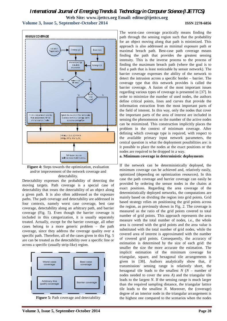
4. THE EVALUATION AND IMPROVEMENT OF MINIMUM COVERAGE The most important parameters and relations in the process of analysis and improvement of minimum coverage are presented in algorithmic form in Fig.5. The deployment environment directly influences the sensing and detection models while the coverage type is defined by the application requirements. After determining the sensing and detection model, assessing the energy model, and defining the deployment model and coverage type for a specific application, different evaluation approaches can be used and different steps can be taken towards the improvement of the minimum coverage depending primarily on the deployment manner and the available nodes. In the process of coverage improvement, if the deployment is deterministic, there is no need for the mobile nodes. On the other hand, if the deployment is stochastic, there are four methods for improving the coverage: by increasing the overall number of nodes or the sensing radius (if possible), by improving the deployment accuracy, or by using mobile nodes. In all cases, after achieving the minimum coverage, some kind of optimization regarding the energy-efficiency, the reliability etc., is often preferable. Before delving into the description of each of the tasks and possibilities, it is important to define the concept of coverage type. The concept of coverage type is tightly related to the concept of area of interest, since it models the applicability of the coverage in accordance to the typical application requirements. Regarding the WSNs applicability, the coverage types are grouped into three main categories: the area coverage, the detectability (and path coverage), and barrier coverage. The area coverage is one of the most interesting coverage types since it is required by most of the WSN-based applications (e.g., in underwater monitoring, military surveillance, environmental monitoring, etc.). This measure is important when the goal is to gather information about the entire region under study.




Figure 4: Steps towards the optimization, evaluation and/or improvement of the network coverage and

detectability. Detectability expresses the probability of detecting the moving targets. Path coverage is a special case of detectability that treats the detectability of an object along a given path. It is also often addressed as the exposure paths. The path coverage and detectability are addressed in four contexts, namely worst case coverage, best case coverage, detectability along an arbitrary path, and barrier coverage (Fig. 5). Even though the barrier coverage is included in this categorization, it is usually separately treated. Actually, except for the barrier coverage, all other cases belong to a more generic problem – the path coverage, since they address the coverage quality over a specific path. Therefore, all of the cases given in this Fig. 5 are can be treated as the detectability over a specific line or across a specific (usually strip-like) region.

Figure 5: Path coverage and detectability

The worst-case coverage practically means finding the path through the sensing region such that the probability for an object moving along that path is minimized. This approach is also addressed as minimal exposure path or maximal breach path. Best-case path coverage means finding the path that provides the greatest sensing intensity. This is the inverse process to the process of finding the maximum breach path (where the goal is to find a path that is least noticeable by sensor network). The barrier coverage expresses the ability of the network to detect the intrusion across a specific border – barrier. The coverage type that this network provides is called the barrier coverage. A fusion of the most important issues regarding various types of coverage is presented in [37]. In order to minimize the number of used nodes, the authors define critical points, lines and curves that provide the information extraction from the most important parts of the field of interest. In this way, only the nodes that cover the important parts of the area of interest are included in sensing the phenomenon so the number of the active nodes can be minimized. This construction implicitly places the problem in the context of minimum coverage. After defining which coverage type is required, with respect to the available primary input network parameters, the central question is what the deployment possibilities are: is it possible to place the nodes at the exact positions or the nodes are required to be dropped in a way. a. Minimum coverage in deterministic deployments

If the network can be deterministically deployed, the minimum coverage can be achieved and, relatively easily, optimized (depending on optimization resources). In this case the path coverage and barrier coverage can easily be provided by ordering the sensor nodes in the chains at exact positions. Regarding the area coverage of the deterministically deployed networks, the computations are mainly based on dividing the region into grid points. Grid based strategy relies on positioning the grid points across the region, as previously shown in Fig. 2. The coverage is measured as the ratio of the grid points covered to total number of grid points. This approach represents the area measure with the total number of nodes, i.e., the whole area is covered with the grid points and the area value is substituted with the total number of grid nodes, while the covered area of interest is approximated with the number of covered grid points. Consequently, the accuracy of estimation is determined by the size of each grid: the smaller the size the more accurate the estimation. The implicit estimation of the minimum coverage for triangular, square, and hexagonal tile arrangements is given in [38]. Authors analytically show that, if transmission/ sensing range is relatively short, the hexagonal tile leads to the smallest N (N – number of nodes needed to cover the area A) and the triangular tile leads to the largest N. If the sensing range is much larger than the required sampling distance, the triangular lattice tile leads to the smallest N. Moreover, the (coverage) degree of an interior node in the triangular arrangement is the highest one compared to the scenarios when the nodes




are positioned in the vertices of some other given geometry. On the other side, the coverage degree is the lowest in the case of hexagon geometry. This means that the triangle tiles lead to the network that has a greater redundancy and hence the greater flexibility for implementation of the various energy-conservation algorithms which consequently has the influence on network lifetime prolongation. The opposite holds for hexagonal arrangement. In general, one can conclude that the best and the worst choice of tiles is either the triangle or hexagon. However, the square has good performance for any of the parameters (such as sensing radius and N). An analysis to covering the strip-like region by using triangular positions of the nodes is given in [39]. The authors assume that each sensor is capable of detecting signals within fixed radius r around it. Sensors are therefore modeled by Boolean model, with radius r as the parameter. Two r-disks are connected if the center of each one falls in the other. The authors cover the region using the node’s placement as depicted in Fig. 6.

Figure 6: A regular deployment method proposed in [39]. Placing the sensors at the depicted positions enables a very high performance ratio for strip-like region coverage. For every even integer k, the centers of the sensor array are

placed at the positions while for every odd integer k, the centers of the sensor array are place at the

positions This placement assures the coverage of the infinite area. The coverage for a region of finite size is derived similarly using the same nodes’ placement. The density of a network deployed this way, i.e., the number of nodes per unit of area, in order for the whole area to be covered, is within 3% of the optimum. The optimum value means the minimum number of nodes to cover the whole area. Here, the actual performance ratio is 1.026. Therefore, the given method is a good approximation of the minimum area coverage by using regular deployment.

Besides placing the nodes at the grid points, in scenarios where the number of nodes need to be reduced, the nodes can be placed at the centre of the cells of the grid structure. An example of the grid based deployment with hexagonal cells, where each cell contains only one node with the probabilistic model being used is given in [40]. Here, the sensing radius may vary from zero to Rmax, where Rmax is the radius of the inscribed circle of hexagonal cell. That means that Rmax is also the height of the rectangles that form the hexagon. Consequently, the area of hexagon

(which is also the probability space of the event), can be presented with respect to Rmax as:

(7) The area that a sensor with sensing radius R covers is the area of circle (Ac) with radius R. That means that the coverage fraction can be approximated with:

(8) This expression reaches the maximum value (90.69%) for R=Rmax. If the number of nodes N can be considered large, the boundary effects are minimal. In that case, the minimum number of nodes needed to cover the circle-like region for R=Rmax and Ra being the radius of the region, can be expressed with:

(9) Similarly, the relations for minimum number of nodes to cover the regions based on triangular and square grids can be derived by using the same methodology. 4.2 Minimum coverage in random deployments In some implementations, the nodes cannot be placed manually at the desired positions. For example, when the terrain is inaccessible, such as in military applications, the implementation can only be achieved in some quasi-random way, such as by using the aircrafts or artillery. As depicted in Fig. 3, in the process of evaluation and/or improvement of any of the coverage type in stochastic implementations, three strategies can be used:

a) Using some of the primary network resources, i.e., varying the number of nodes or adjusting/increasing the sensing radius.

b) Using the mobility in the network. c) Using both strategies a) and b)

4.2.1 Minimum coverage improvement in networks with static nodes only When the network is deployed in some quasi random way, and when it consists of only the static nodes, only some of available network parameters can be changed. In this case, besides making the implementation itself as precise as possible, the designer can only change the network density or the sensing range (if possible). We, hereby, define the network density, the sensing radius and the implementation manner to be the primary network implementation parameters. The network density is often a parameter of choice, i.e., by increasing the number of deployed (static)nodes; one can always improve the network coverage. But, when the sensing radius is much smaller than the dimensions of the area of interest, the significant improvement on sensing coverage can only be achieved by significant increase in number of nodes. Consequently, this would significantly increase the overall cost of the implementation. Moreover, the network cannot be too dense because of the limitations related to the communication and data dissemination, such as spatial




reuse. For example, as presented in [16], the throughput of each of the nodes radically decreases when the network density is increased. Regarding the second parameter, the adjustment of the sensing radius of a node can exponentially improve the minimum coverage or can improve the energy efficiency, but this setup is not always a feasible task. The network deployment manner depends on the available possibilities and the context of application. The evaluation of the minimum coverage of a randomly deployed WSN is either possible to be estimated (if the positions of the nodes are not known after the implementation) or to be computed (if the positions of the nodes are available). The first scenario involves the probability approach while the second uses the methods of computational geometry. In the proceeding discussion, the approaches on evaluation of the minimum network coverage quality for various, most typical coverage types (such as the area coverage, the path coverage, the best case and worst case coverage, and the barrier coverage) are given. By relying on the derived observations, the primary network parameters can possibly be changed for the purpose of improving the minimum coverage to a given extent. When the network is randomly scattered over a region, and when the positions of the nodes are not known after the implementation, the minimum coverage can only be estimated as a probability measure. Let

be the set of nodes whose sensing ranges cover the point P( . The total coverage of the point P, where the influence of all the k sensors is taken into account, can be expressed:

(10) Here, the probability that the point is not covered by any of the nodes is firstly calculated. While the incorporation of the Boolean, Elfe’s, or the general sensing model involves simple sensing patterns (like circles and rings), the shadow-fading or Newman-Pearson models are based on the knowledge of the terrain-specific characteristics for each of the deployed nodes and is never of regular shape. Therefore, let’s consider a more generic situation, where the sensing pattern is not of a circular shape (Fig. 7).

Figure 7: The sensing area is not of a disk-like shape.

If node Si covers the region , and if the area of is , then the probability that an event at the position ( ) will be detected by sensor Si is Ai/A, where A is the whole area of interest. Afterward, the joint probability that a point P is covered by its k neighboring sensors is calculated and it defines the total coverage that the event will be detected by at least one of k nodes. For example, as shown in [40], if Rs and A are the sensing radius and the area of interest, respectively, if the boundary

effects are neglected and the Boolean sensing model is used, the probability that the event will be detected by any arbitrary sensor would be The probability that an event will be detected by at least one of the N nodes is equal to the coverage fraction:

(11) If we denote the network density with λ=N/A, then the above formula can also be expressed as follows:

(12) The relation (12) shows the dependency of the probability of detecting an object in an area on sensing radius and on the network density. Hence, by varying one of these parameters, a certain detection probability level can be estimated. As denoted, another approach for calculating the minimum area coverage (when the positions of the nodes are known) involves the methods of computational geometry. These methods are either based on the Voronoi Diagram or on the Delaunay Triangulation. The Voronoi diagram divides an area into regions around each node, such that the borders of the regions are equidistant from the two nearest nodes (Fig. 8). Each edge of the Voronoi diagram is perpendicular to the line that connects two neighbor nodes. This method is currently frequently used in WSN coverage evaluation and/or improvement [41-46]. Here, every point in a given polygon is closer to the node in this polygon than to any other node. If the area of each i polygon, and the appropriate sensors that belong to that polygon, are denoted with and , respectively, than sensor is the closest sensor to all the points inside the region . If the furthest vertex of the polygon is situated at the distance smaller than sensing radius of the sensor , the polygon is fully covered. If all Voronoi polygons are covered by at least one sensor, the sensing field is covered.

Figure 8: Voronoi diagram in WSN’s coverage.

On the other hand, the Delaunay Triangulation is the geometric dual of the Voronoi Diagram (Fig. 9). It can be defined as a triangulation of the sites with the property that for each triangle, the circumcircle of that triangle is empty of all other sites - nodes.

Figure 9: Delaunay triangulation in WSN’s coverage.




Each edge connects two vertices. For each edge we can find a circle containing the edge's endpoints but not containing any other points. The center of the largest empty circle has the weakest detection probability in a given sensor field. Besides for the purpose of calculations, as will be shown in the proceeding subsection, the approaches based on the Voronoi diagrams and Delaunay triangulation are widely used for improving the area coverage by using the mobility in the network. Another coverage measure is detectability. Detectability is evaluated for the objects that move along a given path in the sensor field. Once again, the detectability can either be estimated by using probability methods or calculated (if the positions of the nodes are known). Regarding the first case, the probability for a node to be positioned at some point of the region is assumed to follow some pre-defined probability distribution curve. For example, by using the presumptions of the relation (6), as described in [47], if we denote the deployment density by and the area of the region by A; than the probability that k sensors will be located in a region A can be described with:

(13) Now, the probability that none of the sensor nodes is within the detecting zone of the path p is:

(14) If the moving trajectories can be interpolated by analytical functions , each with starting and ending points

and , respectively, the detectability of an object moving along the path p will be:

(15) Detectability expresses the ability of the network to detect a moving object along an arbitrary path. As a special case, when the goal is finding a specific path on the network, which is minimally or maximally covered by the sensing field of the network, the detectability problem is addressed as minimal or maximal exposure path. A thorough analyze in minimal exposure path is given in [29]. Here, the authors use the pre-defined all-sensor field intensity and closest-sensor field intensity models in order to find the minimum exposure path for the cases: a) around a single sensor, b) from point p to point q, when p and q are at the equidistance positions from the sensor, c) given a restricted (rectangular) area when a sensor is situated in the center of the rectangle, and d) when the sensor is situated in the centre of a convex polygon’s inscribed circle. Additionally, a generic grid-based approach to practically calculating minimal exposure path is also given in this work. The area is divided using square grids and the exposure is evaluated only at the edges of the grids and/or along the diagonals of grids. As previously denoted, the Voronoi and Delaunay triangulation diagrams are also widely used in in finding the best case coverage (i.e., maximal exposure path) and the worst case coverage (i.e., maximal breach path). A maximal breach path lies on the edges of Voronoi diagram

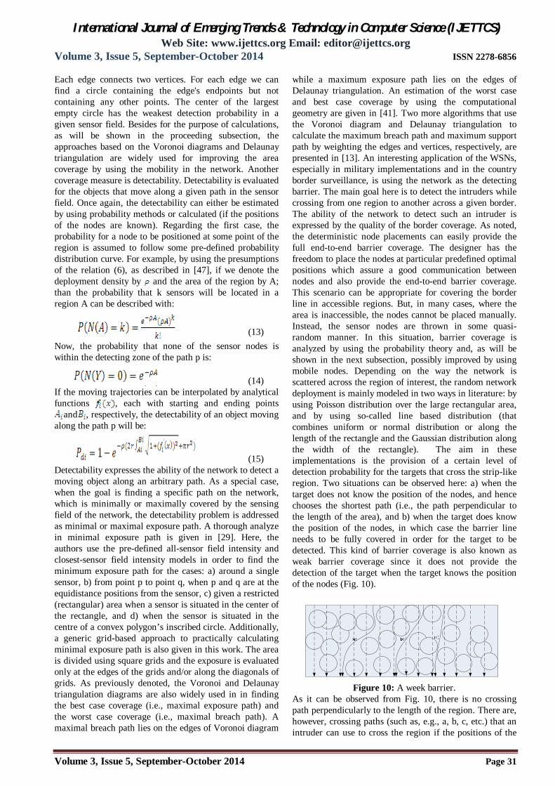
while a maximum exposure path lies on the edges of Delaunay triangulation. An estimation of the worst case and best case coverage by using the computational geometry are given in [41]. Two more algorithms that use the Voronoi diagram and Delaunay triangulation to calculate the maximum breach path and maximum support path by weighting the edges and vertices, respectively, are presented in [13]. An interesting application of the WSNs, especially in military implementations and in the country border surveillance, is using the network as the detecting barrier. The main goal here is to detect the intruders while crossing from one region to another across a given border. The ability of the network to detect such an intruder is expressed by the quality of the border coverage. As noted, the deterministic node placements can easily provide the full end-to-end barrier coverage. The designer has the freedom to place the nodes at particular predefined optimal positions which assure a good communication between nodes and also provide the end-to-end barrier coverage. This scenario can be appropriate for covering the border line in accessible regions. But, in many cases, where the area is inaccessible, the nodes cannot be placed manually. Instead, the sensor nodes are thrown in some quasi-random manner. In this situation, barrier coverage is analyzed by using the probability theory and, as will be shown in the next subsection, possibly improved by using mobile nodes. Depending on the way the network is scattered across the region of interest, the random network deployment is mainly modeled in two ways in literature: by using Poisson distribution over the large rectangular area, and by using so-called line based distribution (that combines uniform or normal distribution or along the length of the rectangle and the Gaussian distribution along the width of the rectangle). The aim in these implementations is the provision of a certain level of detection probability for the targets that cross the strip-like region. Two situations can be observed here: a) when the target does not know the position of the nodes, and hence chooses the shortest path (i.e., the path perpendicular to the length of the area), and b) when the target does know the position of the nodes, in which case the barrier line needs to be fully covered in order for the target to be detected. This kind of barrier coverage is also known as weak barrier coverage since it does not provide the detection of the target when the target knows the position of the nodes (Fig. 10).

Figure 10: A week barrier.

As it can be observed from Fig. 10, there is no crossing path perpendicularly to the length of the region. There are, however, crossing paths (such as, e.g., a, b, c, etc.) that an intruder can use to cross the region if the positions of the




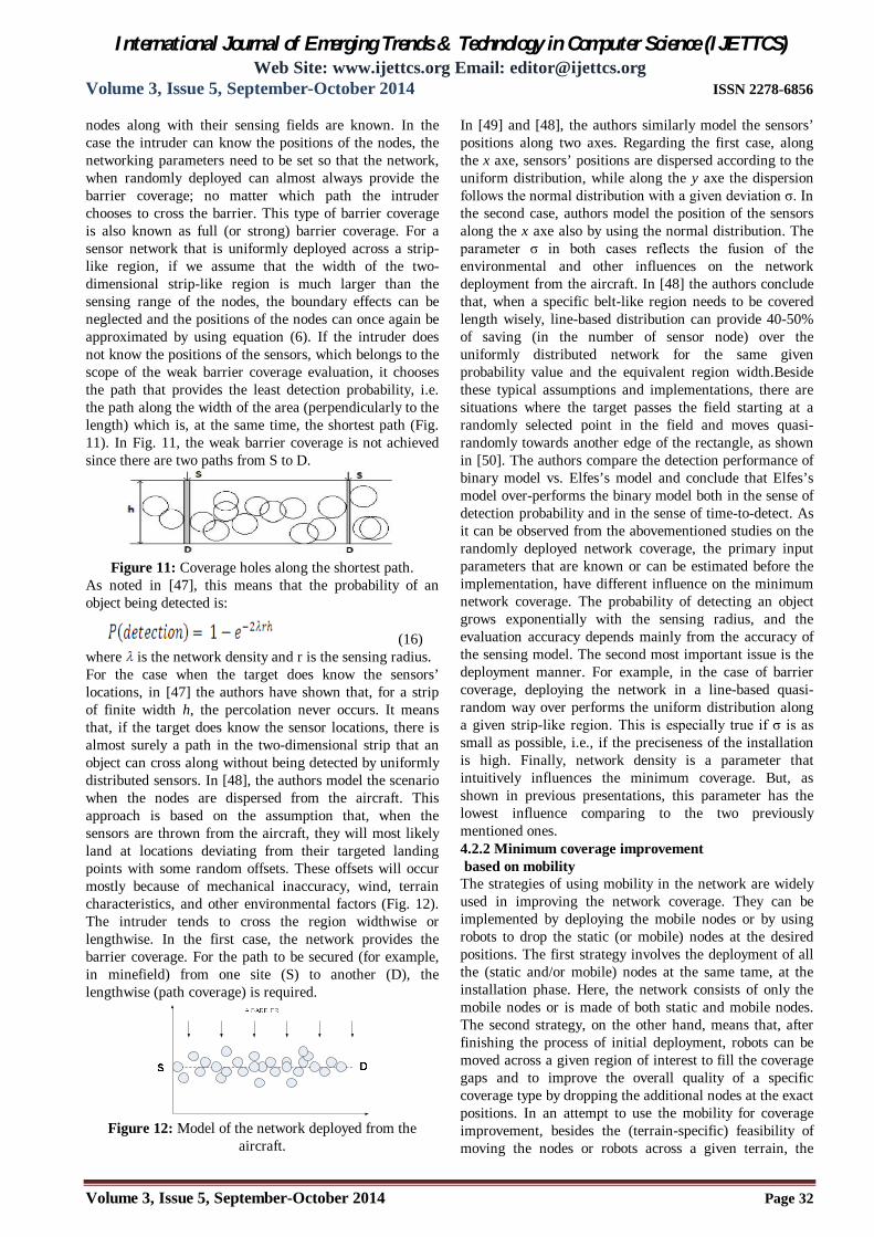
nodes along with their sensing fields are known. In the case the intruder can know the positions of the nodes, the networking parameters need to be set so that the network, when randomly deployed can almost always provide the barrier coverage; no matter which path the intruder chooses to cross the barrier. This type of barrier coverage is also known as full (or strong) barrier coverage. For a sensor network that is uniformly deployed across a strip-like region, if we assume that the width of the two-dimensional strip-like region is much larger than the sensing range of the nodes, the boundary effects can be neglected and the positions of the nodes can once again be approximated by using equation (6). If the intruder does not know the positions of the sensors, which belongs to the scope of the weak barrier coverage evaluation, it chooses the path that provides the least detection probability, i.e. the path along the width of the area (perpendicularly to the length) which is, at the same time, the shortest path (Fig. 11). In Fig. 11, the weak barrier coverage is not achieved since there are two paths from S to D.

Figure 11: Coverage holes along the shortest path.

As noted in [47], this means that the probability of an object being detected is:

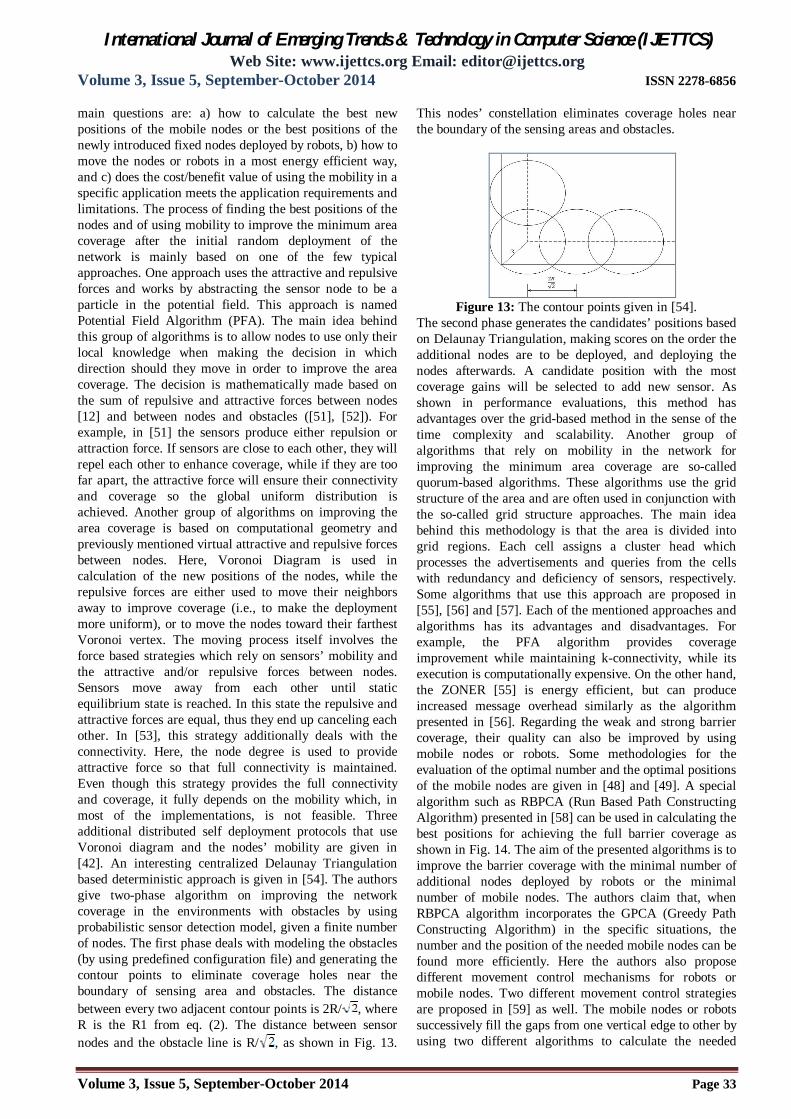
(16) where is the network density and r is the sensing radius. For the case when the target does know the sensors’ locations, in [47] the authors have shown that, for a strip of finite width h, the percolation never occurs. It means that, if the target does know the sensor locations, there is almost surely a path in the two-dimensional strip that an object can cross along without being detected by uniformly distributed sensors. In [48], the authors model the scenario when the nodes are dispersed from the aircraft. This approach is based on the assumption that, when the sensors are thrown from the aircraft, they will most likely land at locations deviating from their targeted landing points with some random offsets. These offsets will occur mostly because of mechanical inaccuracy, wind, terrain characteristics, and other environmental factors (Fig. 12). The intruder tends to cross the region widthwise or lengthwise. In the first case, the network provides the barrier coverage. For the path to be secured (for example, in minefield) from one site (S) to another (D), the lengthwise (path coverage) is required.

Figure 12: Model of the network deployed from the

aircraft.

In [49] and [48], the authors similarly model the sensors’ positions along two axes. Regarding the first case, along the x axe, sensors’ positions are dispersed according to the uniform distribution, while along the y axe the dispersion follows the normal distribution with a given deviation σ. In the second case, authors model the position of the sensors along the x axe also by using the normal distribution. The parameter σ in both cases reflects the fusion of the environmental and other influences on the network deployment from the aircraft. In [48] the authors conclude that, when a specific belt-like region needs to be covered length wisely, line-based distribution can provide 40-50% of saving (in the number of sensor node) over the uniformly distributed network for the same given probability value and the equivalent region width.Beside these typical assumptions and implementations, there are situations where the target passes the field starting at a randomly selected point in the field and moves quasi- randomly towards another edge of the rectangle, as shown in [50]. The authors compare the detection performance of binary model vs. Elfes’s model and conclude that Elfes’s model over-performs the binary model both in the sense of detection probability and in the sense of time-to-detect. As it can be observed from the abovementioned studies on the randomly deployed network coverage, the primary input parameters that are known or can be estimated before the implementation, have different influence on the minimum network coverage. The probability of detecting an object grows exponentially with the sensing radius, and the evaluation accuracy depends mainly from the accuracy of the sensing model. The second most important issue is the deployment manner. For example, in the case of barrier coverage, deploying the network in a line-based quasi-random way over performs the uniform distribution along a given strip-like region. This is especially true if σ is as small as possible, i.e., if the preciseness of the installation is high. Finally, network density is a parameter that intuitively influences the minimum coverage. But, as shown in previous presentations, this parameter has the lowest influence comparing to the two previously mentioned ones. 4.2.2 Minimum coverage improvement based on mobility The strategies of using mobility in the network are widely used in improving the network coverage. They can be implemented by deploying the mobile nodes or by using robots to drop the static (or mobile) nodes at the desired positions. The first strategy involves the deployment of all the (static and/or mobile) nodes at the same tame, at the installation phase. Here, the network consists of only the mobile nodes or is made of both static and mobile nodes. The second strategy, on the other hand, means that, after finishing the process of initial deployment, robots can be moved across a given region of interest to fill the coverage gaps and to improve the overall quality of a specific coverage type by dropping the additional nodes at the exact positions. In an attempt to use the mobility for coverage improvement, besides the (terrain-specific) feasibility of moving the nodes or robots across a given terrain, the




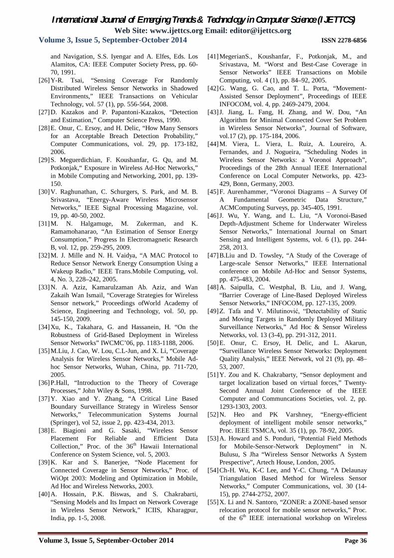
main questions are: a) how to calculate the best new positions of the mobile nodes or the best positions of the newly introduced fixed nodes deployed by robots, b) how to move the nodes or robots in a most energy efficient way, and c) does the cost/benefit value of using the mobility in a specific application meets the application requirements and limitations. The process of finding the best positions of the nodes and of using mobility to improve the minimum area coverage after the initial random deployment of the network is mainly based on one of the few typical approaches. One approach uses the attractive and repulsive forces and works by abstracting the sensor node to be a particle in the potential field. This approach is named Potential Field Algorithm (PFA). The main idea behind this group of algorithms is to allow nodes to use only their local knowledge when making the decision in which direction should they move in order to improve the area coverage. The decision is mathematically made based on the sum of repulsive and attractive forces between nodes [12] and between nodes and obstacles ([51], [52]). For example, in [51] the sensors produce either repulsion or attraction force. If sensors are close to each other, they will repel each other to enhance coverage, while if they are too far apart, the attractive force will ensure their connectivity and coverage so the global uniform distribution is achieved. Another group of algorithms on improving the area coverage is based on computational geometry and previously mentioned virtual attractive and repulsive forces between nodes. Here, Voronoi Diagram is used in calculation of the new positions of the nodes, while the repulsive forces are either used to move their neighbors away to improve coverage (i.e., to make the deployment more uniform), or to move the nodes toward their farthest Voronoi vertex. The moving process itself involves the force based strategies which rely on sensors’ mobility and the attractive and/or repulsive forces between nodes. Sensors move away from each other until static equilibrium state is reached. In this state the repulsive and attractive forces are equal, thus they end up canceling each other. In [53], this strategy additionally deals with the connectivity. Here, the node degree is used to provide attractive force so that full connectivity is maintained. Even though this strategy provides the full connectivity and coverage, it fully depends on the mobility which, in most of the implementations, is not feasible. Three additional distributed self deployment protocols that use Voronoi diagram and the nodes’ mobility are given in [42]. An interesting centralized Delaunay Triangulation based deterministic approach is given in [54]. The authors give two-phase algorithm on improving the network coverage in the environments with obstacles by using probabilistic sensor detection model, given a finite number of nodes. The first phase deals with modeling the obstacles (by using predefined configuration file) and generating the contour points to eliminate coverage holes near the boundary of sensing area and obstacles. The distance between every two adjacent contour points is 2R/ , where R is the R1 from eq. (2). The distance between sensor nodes and the obstacle line is R/ , as shown in Fig. 13.

This nodes’ constellation eliminates coverage holes near the boundary of the sensing areas and obstacles.

Figure 13: The contour points given in [54].

The second phase generates the candidates’ positions based on Delaunay Triangulation, making scores on the order the additional nodes are to be deployed, and deploying the nodes afterwards. A candidate position with the most coverage gains will be selected to add new sensor. As shown in performance evaluations, this method has advantages over the grid-based method in the sense of the time complexity and scalability. Another group of algorithms that rely on mobility in the network for improving the minimum area coverage are so-called quorum-based algorithms. These algorithms use the grid structure of the area and are often used in conjunction with the so-called grid structure approaches. The main idea behind this methodology is that the area is divided into grid regions. Each cell assigns a cluster head which processes the advertisements and queries from the cells with redundancy and deficiency of sensors, respectively. Some algorithms that use this approach are proposed in [55], [56] and [57]. Each of the mentioned approaches and algorithms has its advantages and disadvantages. For example, the PFA algorithm provides coverage improvement while maintaining k-connectivity, while its execution is computationally expensive. On the other hand, the ZONER [55] is energy efficient, but can produce increased message overhead similarly as the algorithm presented in [56]. Regarding the weak and strong barrier coverage, their quality can also be improved by using mobile nodes or robots. Some methodologies for the evaluation of the optimal number and the optimal positions of the mobile nodes are given in [48] and [49]. A special algorithm such as RBPCA (Run Based Path Constructing Algorithm) presented in [58] can be used in calculating the best positions for achieving the full barrier coverage as shown in Fig. 14. The aim of the presented algorithms is to improve the barrier coverage with the minimal number of additional nodes deployed by robots or the minimal number of mobile nodes. The authors claim that, when RBPCA algorithm incorporates the GPCA (Greedy Path Constructing Algorithm) in the specific situations, the number and the position of the needed mobile nodes can be found more efficiently. Here the authors also propose different movement control mechanisms for robots or mobile nodes. Two different movement control strategies are proposed in [59] as well. The mobile nodes or robots successively fill the gaps from one vertical edge to other by using two different algorithms to calculate the needed




positions and by using different moving control mechanisms, until the full barrier coverage is achieved.

Figure 14: A strong WSN-based barrier.

After the initial deployment, the network creates connected graphs and chooses the one with a (run) node closest to the destination border D. In one case this node informs the closest mobile node about the coverage gap, which then inspects the proximity of the run node and, by using one of the criterions, decides where to position itself. After the gap is filled, the connected graph towards destination is prolonged and another run node is chosen. The procedure is repeated for the new node until the graph reaches the edge D. Another case means using robots. In this case, the information from the run node flows to the edge S. Afterward, the robot moves across the region to inspect the proximity of run node. After deploying the nodes to fill the first gap, robot continue to move towards the edge D dropping additional static nodes and making bridges between unconnected graphs towards destination D. A general question in using robots or mobile nodes for the improvement of the coverage is related to the cost-effectiveness of this method over the method which relies on increasing of the number of static nodes. In general, this depends mainly on the terrain of implementation as well as on the cost of the mobile nodes or robots. As observed for the barrier coverage from the construction point of view in [59], the optimal balance between network density and the needed number of additional nodes might be achieved when only few movements are needed and when only one additional node is needed per barrier gap.

5. CONCLUSIONS AND THE FUTURE WORK Although the energy conservation, security, routing and medium access protocols, are very important issues and mostly considered in literature, the coverage and the connectivity remain the fundamental questions that directly express the ability of the WSN-based applications to meet the primary goals such as to detect the events from the field of interest and to communicate the requested information to the user. While taking into account many parameters that limit the applicability of the WSNs, this paper presents the limitations, modeling and the workspace behind the new concept that encapsulates the first core layer of the WSN QoS, i.e., its ability to cover the area of interest in various applications. This new concept is defined to be the minimum coverage. Due to their nature and their behavior in the environment with obstacles, it has been observed that the sensing and

communication field share the similar propagation problems, i.e., their radiating pattern can be modeled similarly. Moreover, under specific conditions, connectivity can be evaluated by using the information about the network coverage and vice versa. Therefore, the concept of minimum coverage can, with some modifications, also be extended to the equivalent concept of minimum connectivity. Although the simplest and consequently the less precise model, when deriving the general knowledge regarding the coverage (and connectivity), the binary sensing/communication model is mostly used, mainly because of the fact that the simplifications, which move the problem to the context of geometric graphs, are mainly based on the disc model. On the other hand, as presented in the paper, other models provide more precise results but are limited to the relatively small number of applications due to their complexity. Besides, covering the area, forming the barrier, or securing a specific path in a deterministically deployed network is more related to the optimizations (regarding the energy consumption, reliability, etc.). Achieving these goals can be resource-constrained but are not influenced or do not influence the minimum coverage. On the other hand, when dealing with the randomly deployed networks, the probabilistic, and sometimes empirical, methods need to be used. In these situations, instead of exact calculation, only the assessment of the coverage quality can be conducted. The improvements in network coverage can be done by increasing one of the network primary parameters (such as number of nodes or the sensing radius) or by using the mobility in the network. The first method is sometimes infeasible or implies high costs; hence the second method is usually a more appropriate one. However, as noted in the paper, the main issue with using the mobility remains the cost-effectiveness of the methods over the ones which rely on the increasing of the number of static nodes or, sometimes, on the change of the sensing radius. After defining the concept itself, this paper provides a more generic design-based and application-centered approach to the evaluation and improvement of the minimum coverage for a wide range of applications. This paper presents, classifies and clusters the critical network parameters in the context of minimum coverage, their influence on the minimum coverage as well as the cross-cluster design-oriented scheme that leads to the approaches for calculation/assessment and the improvement of most typical types of coverage. As such, it aims to serve as a literature-based systemized guideline on establishing the working point of the coverage optimization algorithms in WSN applications. Future research should consider the use of machine learning on the terrain characteristics. The algorithms could enable for the shape and the range model of the sensing pattern to be extracted from the terrain characteristics. This knowledge should greatly contribute to the assessment accuracy. In this direction, future research should include the DTM (Digital Terrain Modeling) techniques to integrate data (regarding the geographic shapes) into the deployment and sensing models, especially when the network is supposed




to be deployed randomly. After defining the shapes and content of the terrain by using segmentation and the multimedia data extraction [60], conceptual modeling could also be used in presenting the relations between the various environmental and deployment factors and their influence to the network modeling and simulation environment. This should lead to adaptive modeling of the WSN implementations and consequently to the more accurate network coverage assessments and improvements. While relying on the pathways given in this paper, another research will continue in the direction of the higher layers in WSN efficiency, i.e., in clustering and classification of the energy-aware coverage algorithms which do not consider the minimum coverage as achieved.

References

[1] X. Wang, G. Xing, Y. Zhang, C. Lu, R. Pless, and C. Gill, “ Integrated Coverage and Connectivity in Wireless Sensor Networks,” Proceedings of the 1st International Conference on Embedded Sensor Systems, pp. 28-39, 2003.

[2] M. Cardei, M. Thai, L. Yingshu, and W. Weili, “Energy Efficient Target Coverage in Wireless Sensor Networks,” Proc. of 24th Annual Joint Conference of the IEEE Computer and Communications Societies, vol. 3, pp. 1976-1984, 2005.

[3] C-C. Hung, W-C. Peng, W-C. Lee, “Energy-Aware Set-Covering Approaches for Approximate Data Collection in Wireless Sensor Networks,” IEEE Trans. Knowl. Data Eng. 24(11), 2012.

[4] F. Pedraza, A. L. Medaglia, and A. Garcia, “Efficient Coverage Algorithms for Wireless Sensor Networks,” IEEE Systems and Information Engineering Design Symposium, pp. 78-83, 2006.

[5] M. Cardei and D. Du, “Improving Wireless Sensor Network Lifetime through Power Aware Organization,” Wireless Networks, vol. 11 (3), 2005.

[6] H. Zhang, H. Wang, and H. Feng, “A Distributed Optimum Algorithm for Target Coverage in Wireless Sensor Networks,” Asia-Pacific Conference on Information Processing, 2009.

[7] A. Cerpa and D. Estrin, “ASCENT: Adaptive Self-Configuring sEnsor Networks Topologies,” IEEE Transactions on Mobile Computing, vol. 3 (3), pp. 272-285, 2004.

[8] M. Hefeeda and M. Bagheri, “ Randomized k-coverage Algorithms for Dense Sensor Networks,” in Proc. of Internetional Conference on Computer Communications and Networks (ICCCN ’04), Chicago, IL, 2004.

[9] J. Liu, X. Kuotsoukos, J. Reich, and F. Zhao, “Sensing Field Characterization in Distributed Sensor Network,” IEEE International Conference on Acoustics, Speech, and Signal Processing, pp. 173-176, 2003.

[10] H. Zhang and J. Hou, “Maintaining Sensing Coverage and Connectivity in Large Sensor Networks,” Wireless

Ad Hoc and Sensor Networks, vol. 1 (1-2), pp. 89-124, 2005.

[11] J. Carle and D. Simplot-Ryl, “Energy Efficient Area Monitoring for Sensor Networks,” IEEE Computer Society, February, vol. 37 (2), pp. 40-46, 2004.

[12] S. Poduri and G. S. Sukhatme, “Constrained Coverage for Mobile Sensor Networks,” Proc. on Robotics and Automation, vol. 1, pp. 165-171, 2004.

[13] S. Meguerdichian, F. Koushanfar, M. Potkonjak, and M. Srivastava, “Coverage Problems in Wireless Ad-Hoc Sensor Networks,” IEEE Infocom, vol.3, pp. 1380-1387, 2001.

[14] L. Wang and Y. Xiao, “A Survey of Energy-Efficient Scheduling Mechanisms in Sensor Networks,” Special Issue on selected papers from IEEE Broadnets, vol. 11 (5), pp. 723-740, 2006.

[15] G. Fan and S. Jin, “Coverage Problem in Wireless Sensor Network: A Survey,” Journal of Networks, vol. 5 (9), pp. 1033-1040, 2010.

[16] S. Commuri and M. K. Watfa, “Coverage Strategies in Wireless Sensor Networks,” International Journal of Distributed Sensor Networks, no. 2, pp. 333-353, 2006.

[17] S. Sangeetha and R. Lakmshmi, “A Survey on Coverage Problems in Wireless Sensor Networks,” International Journal of Advanced Research in Computer Engineering & Technology, vol. 1 (10), 2012.

[18] D.F. Huang and Y.C Tseng, "The Coverage Problem in Three Dimensional Wireless Sensor Networks." GLOBECOM'04: IEEE Global Telecommunications Conf., pp. 3182-3186, 2004.

[19] D. Tian and N. D. Georganas, “A Coverage Preserving Node Scheduling Scheme for Large Wireless Sensor Networks,” in First ACM InternationalWorkshop on Wireless Sensor Networks and Applications, pp. 32–41, 2002.

[20] F. Ye, G. Zhong, S. Lu, and L. Zhang, “Peas: A Robust Energy Conserving Protocol for Long-lived Sensor Networks,” in Proc. ICDCS, pp. 28-37, 2003.

[21] S. Shakkottai, R. Srikant, and N. Shroff, “Unreliable Sensor Grids: Coverage, Connectivity and Diameter,” in Proc. IEEE Infocom, vol.2, pp. 1073-1083, 2003.

[22] M. Hata, “Empirical Formula for Propagation Loss in Land Mobile Radio Services,” IEEE Transactions on Vehicular Technology, vol. 29, pp. 317–325, 1980.

[23] D. Li, K. Wong, Y. Hu, and A. Sayeed, “Detection, Classification, Tracking of Targets in Micro-Sensor Networks,” in IEEE Signal Processing Magazine, 2002.

[24] M. Chu, H. Haussecker, and F. Zhao, “Scalable Information-Driven Sensor Querying and Routing for Ad Hoc Heterogeneous Sensor Networks,” International Journal on High Performance Computing Applications, vol. 16 (3), pp. 293-313, 2002.

[25] A. Elfes, “Occupancy Grids: A Stochastic Spatial Representation for Active Robot Perception,” in Autonomous Mobile Robots: Perception, Mapping,




and Navigation, S.S. Iyengar and A. Elfes, Eds. Los Alamitos, CA: IEEE Computer Society Press, pp. 60-70, 1991.

[26] Y-R. Tsai, “Sensing Coverage For Randomly Distributed Wireless Sensor Networks in Shadowed Environments,” IEEE Transactions on Vehicular Technology, vol. 57 (1), pp. 556-564, 2008.

[27] D. Kazakos and P. Papantoni-Kazakos, “Detection and Estimation,” Computer Science Press, 1990.

[28] E. Onur, C. Ersoy, and H. Delic, “How Many Sensors for an Acceptable Breach Detection Probability,” Computer Communications, vol. 29, pp. 173-182, 2006.

[29] S. Meguerdichian, F. Koushanfar, G. Qu, and M. Potkonjak,“ Exposure in Wireless Ad-Hoc Networks,” in Mobile Computing and Networking, 2001, pp. 139-150.

[30] V. Raghunathan, C. Schurgers, S. Park, and M. B. Srivastava, “Energy-Aware Wireless Microsensor Networks,” IEEE Signal Processing Magazine, vol. 19, pp. 40-50, 2002.

[31] M. N. Halgamuge, M. Zukerman, and K. Ramamohanarao, “An Estimation of Sensor Energy Consumption,” Progress In Electromagnetic Research B, vol. 12, pp. 259-295, 2009.

[32] M. J. Mille and N. H. Vaidya, “A MAC Protocol to Reduce Sensor Network Energy Consumption Using a Wakeup Radio,” IEEE Trans.Mobile Computing, vol. 4, No. 3, 228–242, 2005.

[33] N. A. Aziz, Kamarulzaman Ab. Aziz, and Wan Zakaih Wan Ismail, “Coverage Strategies for Wireless Sensor network,” Proceedings ofWorld Academy of Science, Engineering and Technology, vol. 50, pp. 145-150, 2009.

[34] Xu, K., Takahara, G. and Hassanein, H. “On the Robustness of Grid-Based Deployment in Wireless Sensor Networks” IWCMC’06, pp. 1183-1188, 2006.

[35] M.Liu, J. Cao, W. Lou, C.L-Jun, and X. Li, “Coverage Analysis for Wireless Sensor Networks,” Mobile Ad-hoc Sensor Networks, Wuhan, China, pp. 711-720, 2005.

[36] P.Hall, “Introduction to the Theory of Coverage Processes,” John Wiley & Sons, 1998.

[37] Y. Xiao and Y. Zhang, “A Critical Line Based Boundary Surveillance Strategy in Wireless Sensor Networks,” Telecommunication Systems Journal (Springer), vol 52, issue 2, pp. 423-434, 2013.

[38] E. Biagioni and G. Sasaki, “Wireless Sensor Placement For Reliable and Efficient Data Collection,” Proc. of the 36th Hawaii International Conference on System Science, vol. 5, 2003.

[39] K. Kar and S. Banerjee, “Node Placement for Connected Coverage in Sensor Networks,” Proc. of WiOpt 2003: Modeling and Optimization in Mobile, Ad Hoc and Wireless Networks, 2003.

[40] A. Hossain, P.K. Biswas, and S. Chakrabarti, “Sensing Models and Its Impact on Network Coverage in Wireless Sensor Network,” ICIIS, Kharagpur, India, pp. 1-5, 2008.

[41] MegerianS., Koushanfar, F., Potkonjak, M., and Srivastava, M. “Worst and Best-Case Coverage in Sensor Networks” IEEE Transactions on Mobile Computing, vol. 4 (1), pp. 84–92, 2005.

[42] G. Wang, G. Cao, and T. L. Porta, “Movement-Assisted Sensor Deployment”, Proceedings of IEEE INFOCOM, vol. 4, pp. 2469-2479, 2004.

[43] J. Jiang, L. Fang, H. Zhang, and W. Dou, “An Algorithm for Minimal Connected Cover Set Problem in Wireless Sensor Networks”, Journal of Software, vol.17 (2), pp. 175-184, 2006.

[44] M. Viera, L. Viera, L. Ruiz, A. Loureiro, A. Fernandes, and J. Nogueira, “Scheduling Nodes in Wireless Sensor Networks: a Voronoi Approach”, Proceedings of the 28th Annual IEEE International Conference on Local Computer Networks, pp. 423-429, Bonn, Germany, 2003.

[45] F. Aurenhammer, “Voronoi Diagrams – A Survey Of A Fundamental Geometric Data Structure,” ACMComputing Surveys, pp. 345-405, 1991.

[46] J. Wu, Y. Wang, and L. Liu, “A Voronoi-Based Depth-Adjustment Scheme for Underwater Wireless Sensor Networks,” International Journal on Smart Sensing and Intelligent Systems, vol. 6 (1), pp. 244-258, 2013.

[47] B.Liu and D. Towsley, “A Study of the Coverage of Large-scale Sensor Networks,” IEEE International conference on Mobile Ad-Hoc and Sensor Systems, pp. 475-483, 2004.

[48] A. Saipulla, C. Westphal, B. Liu, and J. Wang, “Barrier Coverage of Line-Based Deployed Wireless Sensor Networks,” INFOCOM, pp. 127-135, 2009.

[49] Z. Tafa and V. Milutinović, “Detectability of Static and Moving Targets in Randomly Deployed Military Surveillance Networks,” Ad Hoc & Sensor Wireless Networks, vol. 13 (3-4), pp. 291-312, 2011.

[50] E. Onur, C. Ersoy, H. Delic, and L. Akarun, “Surveillance Wireless Sensor Networks: Deployment Quality Analysis,” IEEE Network, vol 21 (9), pp. 48–53, 2007.

[51] Y. Zou and K. Chakrabarty, “Sensor deployment and target localization based on virtual forces,” Twenty-Second Annual Joint Conference of the IEEE Computer and Communcations Societies, vol. 2, pp. 1293-1303, 2003.

[52] N. Heo and PK Varshney, “Energy-efficient deployment of intelligent mobile sensor networks,” Proc. IEEE TSMCA, vol. 35 (1), pp. 78-92, 2005.

[53] A. Howard and S. Ponduri, “Potential Field Methods for Mobile-Sensor-Network Deployment” in N. Bulusu, S Jha “Wireless Sensor Networks A System Prespective”, Artech House, London, 2005.

[54] Ch-H. Wu, K-C Lee, and Y-C. Chung, “A Delaunay Triangulation Based Method for Wireless Sensor Networks,” Computer Communications, vol. 30 (14-15), pp. 2744-2752, 2007.

[55] X. Li and N. Santoro, “ZONER: a ZONE-based sensor relocation protocol for mobile sensor networks,” Proc. of the 6th IEEE international workshop on Wireless




Local Networks (WLN), Carleton University, Ottawa, pp. 923-930, 2006.

[56] X. Li, N. Santoro, and I. Stojmenovic, “Mesh-based sensor relocation for coverage maintenance in mobile sensor networks,”in Proc.of 4th international conference on Ubiquitous Intelligence and Computing (UIC), pp. 696-708, 2007.

[57] S. Yang, L. Minglu, and J. Wu, “Scan-based movement-assisted sensor deployment methods in wireless sensor networks,” IEEE Transactions on Parallel Distributed Systems, vol. 18 (8), pp. 1108-1121, 2007.

[58] Z. Tafa, “Robot-Assisted Algorithms on Providing Path Connectivity and Barrier Coverage in Stochastic Network Deployments”, Third International ICST Conference on Ad Hoc Networks, Paris, France, 2011.

[59] Z. Tafa, “Towards Improving Barrier Coverage Using Mobile Robots,” Proc. of IEEE Mediterranean Conference on Embedded Computing, Bar, Montenegro, pp. 166-169, 2012.

[60] S. Vrochidis, C. Doulaverakis, A. Gounaris, E. Nidelkou, and Y. Kompatsiaris, “A Hybrid Ontology and Visual-Based Retrieval Model for Cultural Heritage Multimedia Collections,” International Journal on Metadata Semantics and Ontologies, vol.3 (3), pp. 167-182, 2008.

AUTHOR

Zhilbert Tafa received his Ph.D. in electrical engineering from U. of Belgrade. Currently he is on the faculty of Computer Science and Engineering,

University for Business and Technology in Prishtina. He has published a number of SCI papers, conference papers, and book chapters

minimum coverage design in wireless surveillance networks

Documents