area coverage algorithms for multiagent … for software systems area coverage algorithms for...
TRANSCRIPT

Institute for Software Systems
Area Coverage Algorithms forMultiagent Surveillance Tasks
Master Thesis
Author: Pavichaya EaungpulswatSupervisors: Prof. Dr. Ralf Möller
Prof. Dr. Herbert Werner
May 21, 2012


Declaration
I hereby assert that this thesis has been compiled by me with only the help of the auxil-iary material listed in the text or in the bibliography.
Hamburg, May 21, 2012
Pavichaya Eaungpulswat
iii


Contents
1 Introduction 3
2 Non-Communicative Area Coverage 62.1 Area Decomposition . . . . . . . . . . . . . . . . . . . . . . . . . . . 7
2.1.1 Relative Capabilities of the UAVs . . . . . . . . . . . . . . . . 72.1.2 Algorithm . . . . . . . . . . . . . . . . . . . . . . . . . . . . . 8
2.2 Individual Areas Coverage . . . . . . . . . . . . . . . . . . . . . . . . 112.2.1 Sensing Capabilities . . . . . . . . . . . . . . . . . . . . . . . 112.2.2 Optimal Line Sweep Decompositions . . . . . . . . . . . . . . 13
3 Geometry-Based Area Decomposition 163.1 Decomposition Algorithm . . . . . . . . . . . . . . . . . . . . . . . . 173.2 Algorithm Analysis . . . . . . . . . . . . . . . . . . . . . . . . . . . . 203.3 Area Coverage Redundancy . . . . . . . . . . . . . . . . . . . . . . . 243.4 Discussion and Results . . . . . . . . . . . . . . . . . . . . . . . . . . 26
4 Communicative Area Coverage 294.1 Static Positioning of Nodes . . . . . . . . . . . . . . . . . . . . . . . . 30
4.1.1 Minimum number of nodes . . . . . . . . . . . . . . . . . . . . 314.2 Dynamic Repositioning of Nodes . . . . . . . . . . . . . . . . . . . . . 36
4.2.1 Distributed Self-Spreading Algorithm (DSSA) . . . . . . . . . 374.2.2 VD-Based Deployment Algorithm (VDDA) . . . . . . . . . . . 424.2.3 The Centroid-based Scheme . . . . . . . . . . . . . . . . . . . 47
4.3 Simulation Results and Analysis . . . . . . . . . . . . . . . . . . . . . 48
5 Conclusion and Future Work 56
List of Figures 61
Bibliography 64
v


Abstract
This thesis presents algorithms for area coverage in non-communicative and commu-nicative surveillance tasks using a team of unmanned aerial vehicles (UAVs). In non-communicative tasks, the UAV agents sweep back and forth over a region of interest toperform area coverage. The polygon area decomposition and individual areas coveragealgorithms are presented. The algorithms are intended for a situation where the UAVagents have to start and end area coverage at the same base station. In communicativearea coverage, the methods for static node positioning and dynamic node repositioningare presented. The algorithms for dynamic repositioning are applied to assist a situationwhere the nodes are at the predetermined locations from static positioning, but thereis one or more missing nodes in the region of interest. The results and analysis of thealgorithms on the given situation is presented.
1


Chapter 1
Introduction
The area coverage problem in this thesis is divided into area coverage without communi-cation (non-communicative) and area coverage with communication (communicative).The purpose of both area coverage is to sense a region of interest with equipped cameraor other type of sensor. The agent may take a video or pictures of an observed region toprovide an efficient overview to a base station. The applications for area coverage aresuch as forest fire monitoring, military surveillance, aerial mapping, private security,and other remote surveillance tasks.
Unmanned aerial vehicles (UAVs) can be used in area coverage tasks. They are some-times preferred over manned aircraft in a task such as a routine or risky surveillancemission. The UAVs are relatively inexpensive, have smaller size than manned aircraft,and can be used to minimize the cost of the mission.
This thesis concerns cooperative area coverage operation of multi-agent. Multiple UAVsare used to perform the tasks cooperatively. They enhance the effectiveness of the tasksin large area coverage and explore different aspect of locations at the same time.
When the number of UAV agents is limited and is not enough to entirely cover a re-gion of interest, offline path planning is used for area coverage. The task for each agentis subdivided disjointedly. Each agent performs area coverage task by sweeping andsensing its assigned region. A team of agent cooperates to complete the task as quicklyas possible.
The UAV agent sweeps back and forth to cover its region. The back and forth mo-tion contains sharp turns and is not applicable in fixed wing UAVs, since the fixed wingaircrafts are restricted to constant forward movement. They cannot make sharp turns,or stop and maintain a specific position. Quadrotor, on the other hand, has the ability tohover in place, make tight turns, and move in any direction [10]. Nevertheless, when the
3

Chapter 1: Introduction 4
route contains sharp turns, turning would require the quadrotor to slow to a halt at sharpcorners [16]. An example from [4] shows that moving a quadrotor along the shortestsafe path with sharp corners requires more time than moving along the free path of thequadrotor. Hence, the number of sharp turns is related to the amount of time used inperforming area coverage.
The area coverage route should not overlap and should lead to the complete area cover-age with minimum time and energy. Overlapped area or area redundancy occurs whena location has been visited by one of the agents and is visited again by the same or dif-ferent agent in the team. This wastes time and energy consumption in the mission. Theestimated lifetime of the agents is determined from the amount of battery remaining inthe agents.
Considering an environment where a group of agents assembles at a base station, areacoverage algorithm should start and end at the same position. The problem then arisesas in which way to divide an area and how to allocate the subareas to the agents. Apolygon area decomposition problem presented in [15] is used to solve the problem.In addition, another area decomposition algorithm is proposed aiming to improve areacoverage performance of the UAVs.
In this thesis, the region of interest in a disaster area or where there is no network-ing infrastructure is assumed. When the number of agents is not enough to spread overthe region, the agents have to perform area coverage non-communicatively. However,when there are enough agents to entirely cover the region of interest, mobile ad hocnetwork (MANET) can be applied and communication is possible.
In area coverage with communication, the agents can communicate among themselvesand to the base station. The agents are positioned that the base station and all the agentsstay connected during the mission. Each agent senses its own region and sends the databack to the base station. This area coverage allows the surveillance to last longer thanarea coverage that sweeps along the region, since each agent observes only one location.The communicative area coverage requires more number of agents, however, it gives thebase station near real-time surveillance data.
The node positioning in this area coverage is divided into static positioning where thelocations are predetermined from the base station and dynamic repositioning where theagents determine their locations autonomously. Dynamic repositioning can be used toassist area coverage when the nodes are randomly dispersed or when a region of interestis not entirely covered.

Chapter 1: Introduction 5
The outline of this thesis is as follows: section 2 presents non-communicative area cov-erage with relative and sensing capabilities of the UAVs and decomposition algorithm.Section 3 introduces a proposed area decomposition algorithm based on geometry ofpolygon and required subareas. Section 4 presents communicative area coverage wherethe agents and base station are connected. Conclusion and future work is presented insection 5.

Chapter 2
Non-Communicative Area Coverage
This section presents area coverage for multi-agent surveillance tasks where each agentperforms its task disjointedly. Each agent is responsible only for its divided area and allthe information from each agent are combined for an image of the entire area. The datasuch as assigned area and a route for each agent is calculated by the base station beforethe task start. During the task, an agent simply follows the predetermined route of itsassigned region with the use of built-in Global Positioning System (GPS).
Maza and Ollero [22] have presented the problem of cooperatively searching a givenarea to detect objects of interest, using a team of heterogenous UAVs. The problem theyhave presented can be applied to an area coverage problem for multiagent surveillancetasks, as the function of the two tasks are related. Their algorithms start with assigninga region for each UAV, and then covering a region using a zigzag pattern.
An assigned region is derived according to an area decomposition algorithm. The regionis partitioned from an entire area considering factors such as initial coordinates, cameraangles, sensing width and relative capabilities of the UAV agent. The area partition usedin this section is from area decomposition algorithm by Hert and Lumelsky [15].
After the subregion for an agent is assigned, a route within the sub-region is deter-mined. The route is obtained regarding to the shape of the assigned region by finding adirection that yields minimum diameter function. Then the agent sweeps towards thatdirection using back and forth motion to entirely cover its assigned region. The sweepdirection used for the route finding in this part is introduced by Huang [17].
An area decomposition including relative capabilities of the agents and a decomposi-tion algorithm is presented in section 2.1. Section 2.2 presents individual area coverageincluding sensing capabilities and optimal line sweep decompositions.
6

2.1 Area Decomposition 7
2.1 Area Decomposition
The area decomposition problem is the problem of dividing a given area into a set ofsmaller subregions. There are various algorithms for area or task decomposition. Thesealgorithms vary upon the shape of the environment and the divided subregions. For ex-ample, there is an algorithm for multiple UAVs area coverage in an arbitrary rectilinearworkspace [1]. This partitioning algorithm is therefore divides a workspace into n con-tiguous rectilinear parts whose areas are in a pre-specified ratio. For general polygonenvironments, the most common and widely applicable form of polygon decompositionis triangulation. These decompositions create triangulations of polygons with variouscharacteristics as can be seen in [6] [8] [9]. Apart from triangulation, the polygons canbe decomposed into trapezoids [2], convex polygons [5] [11] [18] [25], star-shaped ormonotone polygons [18], and rectangles [21].
In this thesis, the interested area partition problem is the one that divides a given ar-bitrary convex polygon into a number of convex pieces, each with a given area. Thenumber of convex pieces varies according to the number of agents available for areacoverage. The size of the divided area varies according to relative capabilities of eachagent. The capabilities considered in area partition are such as flight speed, battery life-time, and width of camera’s view of the UAV agent.
Section 2.1.1 presents the relative capabilities of the UAVs which describes the dif-ference between each agent. Section 2.1.2 presents a polygon area decomposition al-gorithm. The algorithm partitions a polygon according to required areas and startingpoints of the UAV agents.
2.1.1 Relative Capabilities of the UAVs
As the multiagents considered in this thesis are a set of small quadrotors, the capabilityof each agent is confined by its specifications such as weight, battery lifetime, payload,and sensors specifications. These factors strongly influence the agent’s maximum flyingrange which is one of the fundamental measurements for the agent’s capability. As theUAVs can be heterogeneous, the other factors namely flight speed, sensitivity to windconditions, altitude required for the mission, and sensing width due to different cam-era’s fields of view for each UAVs should also be taken into account.
The sensing width depends on the UAV’s specification and also varies according tothe flying altitude of the agents. The camera sensor has a bigger sensing width as the

2.1 Area Decomposition 8
UAV flies at higher altitude above the ground. Nevertheless, it gives poorer image qual-ity for further processing. The flying altitude of a UAV depends on the purpose of themultiagent mission, and situation of that moment e.g. the wind condition. One have tochoose whether to have a finer image quality or a larger sensor range.
Based on the relative capabilities of the agents, the proportions of the area of the re-gion P are determined in order to assign them to each agent. These proportions arerepresented by a set of values ci where i = 1, ...,n and n is the number of UAV agents,with
0 < ci < 1 andn
∑i=1
ci = 1.
Therefore, the problem considered is as follows: Given a polygon P and n starting points(sites) S1, · · · ,Sn on the polygon, divide the polygon into n nonoverlapping polygonsP1, · · · ,Pn such that
Area(Pi) = ci×Area(P) and Si is on Pi.
2.1.2 Algorithm
This area decomposition algorithm is presented by Hert and Lumelski [15]. It usessweep-line and divide-and-conquer techniques to construct a polygon partition. Thearea partition problem is constrained by area requirements of each subregion and start-ing position of each agent.
In an area partition of a polygon P, a set of nonoverlapping sub-polygons P1, ...,Pn witha specified area and a set of start positions of the agent for performing area coverageS1, ...,Sn are divided. Each polygon Pi consists of a particular point Si on the border ofPi. For each start position Si, an area requirement or desired area of each polygon Pi isdenoted by AreaRequired(Si).
In the problem, AreaRequired(Si) = ci× Area(P) where 0 < ci < 1 and ∑ni=1 ci = 1
is considered. Furthermore, for any set of start position S,
AreaRequired(S) = ∑AreaRequired(Si).
For the area partition of n agents, the desired subregions can be achieved using n− 1

2.1 Area Decomposition 9
line segments or the area partition algorithm has to perform n−1 times.
Let L = (Ls,Le) denotes a line segment oriented from Ls to Le dividing the polygonP into two convex pieces. Pr
L is a convex polygon to the right of L and PlL is the com-
plement of PrL; P−Pr
L. The algorithm for dividing a simply connected, convex polygoninto two smaller regions is as follow:
Algorithm 1 Divide a convex polygon into two smaller polygons [15]
Input:
convex polygon P;the list of vertices and start positions W (P) = wk, k = 1, ...,m in CCW order;the set of start positions S(P) = S1, ...,Sn numbered according to their orderin the list W (P)
Output: two polygons PlL and Pr
L
1. Assume S1 = wk; L← (w1,wk)
2. S(PrL)←{S1}
3. while Area(PrL)< AreaRequired(S(Pr
L)) and Le 6= Sn dok← k+1Le← wk
end while4. if Le = S1 and Area(Pr
L)> AreaRequired(S(PrL)) then
Move Ls CCW along PrL until Area(Pr
L) = AreaRequired(S(PrL))
else if Le = Sn and Area(PrL)< AreaRequired(S(Pr
L)) thenMove Ls CW along P until Area(Pr
L) = AreaRequired(S(PrL))
elseInterpolate Le CW until Area(Pr
L) = AreaRequired(S(PrL))
end if
5. PlL = P−Pr
L
6. L = (Ls,Le)

2.1 Area Decomposition 10
Figure 2.1: Steps for polygon area decomposition. In this figure, the polygon is dividedinto three polygons with equal areas

2.2 Individual Areas Coverage 11
Algorithm 1 summarizes the procedure for dividing a given convex polygon P into twosmaller polygons. The steps are visually presented in figure 2.1. In the figure, a givenconvex polygon is considered as the interested region for area coverage and there arethree UAV agents performing the task. Figure (a) shows a convex polygon P with fivevertices w1,w2,w3,w4,w8 and start positions of the three UAVs S1,S2,S3 or w5,w6,w7.Figure (b) shows the polygon P with line segment L = (Ls,Le) initialized as the segment(w1,w5). Then it checks whether the area of polygon Pr
L(w1,w2,w3,w4,w5) is smalleror bigger than the required area. If the area of Pr
L is bigger, moves Ls from w1 counterclockwise along the polygon P until the area Pr
L is equal to the required area. If the areaof Pr
L is smaller, then moves Ls clockwise. Figure (c) shows the line segment L=(Ls,Le)that makes area of Pr
L equal to the required area. According to Algorithm 1, the polygonarea decomposition has completed its task in dividing a polygon P into two smallerpolygons. Yet, three polygons are needed for area coverage task. The algorithm has tobe repeated for a convex polygon Pl
L(w1,w2,w3,w6). Figure (d) shows a decompositionof convex polygon Pl
L. Line segment L is initialized as the segment (w1,w4). Figure (e)shows the complete polygon area decomposition where the polygon P is divided equallyinto three polygons.
2.2 Individual Areas Coverage
Once the desired subregion is divided for each UAV, the path for covering each sub-region is needed for the agent to perform area coverage. The path for individual areacoverage is based on the shape of the subregion and sensing capability of the agent.Section 2.2.1 presents the sensing capabilities of the agents and their resulting sensingwidths. Section 2.2.2 presents the path for covering a subregion using back and forthmotion.
2.2.1 Sensing Capabilities
To examine a region of interest, a team of UAVs have to perform a cooperative searchoperation over the region. Each UAV is equipped with sensors or cameras. The sensorsallow the vehicles to determine their own coordinates relative to a Base Coordinate Sys-tem (BCS) and the coordinates of points detected in their sensing regions. The BCS isfixed in the environment defining x-axis towards north, y-axis towards west, and z-axispoints upward.
Each UAV has associated an UAV Coordinate System (UCS); x-axis forward, y-axis

2.2 Individual Areas Coverage 12
left, z-axis up. When a vehicle moves, the starting point and orientation of the UAVchange. A fixed on board camera in each UAV can orient in x− z plane of the UCS. Theorientation is defined by an angle −α with respect to the x-axis.
As the UAV moves along a defined path, it takes shots or video over an interested re-gion. An imaged area on the terrain is defined from the image pyramid of the camera asshown in figure 2.2. Considering a plain terrain, it can be shown that the sensing widthof an UAV moving in the x− z plane of the UCS is given by [22]:
w = 2zBCS tanγ[sinα + cosα tan(π
2−α−β )] (2.1)
where zBCS is the altitude of the UAV, and angles β and γ determine the field of view ofthe camera.
To generalize the planar algorithm in equation 2.1, the non-planar surface in three-dimensional environment is considered. The area to be covered must be a verticallyprojectively planar surface; a vertical line passing through any point on the surface in-tersects it at only one point.
Figure 2.2: The imaged area is the intersection of the image pyramid and the terrain[22].

2.2 Individual Areas Coverage 13
2.2.2 Optimal Line Sweep Decompositions
Subregions can be covered by sweeping the agents using back and forth motion. Thiscoverage can be improved by determining the optimal sweep direction. The optimal linesweep decompositions presented by Huang [17] is used to optimize the amount of timeused in individual area coverage. The method finds the route direction that minimizesthe number of turns when performing area coverage.
Since this area coverage path contains sharp turns, the UAV requires more time whenturning comparing to going straight. When turning, the UAV needs to slow down, stayhovering, make the turn, and then accelerate again for efficient area coverage. Accord-ingly, finding the path that minimizes the number of turns reduces the coverage time asillustrated in Figure 2.3. The figure shows that different sweep direction can result inlarge difference in number of turns, even though the total length is the same.
Figure 2.3: The number of turns is different as the agent moves along different sweepdirections. This results in different amount of time needed for covering a region [17].
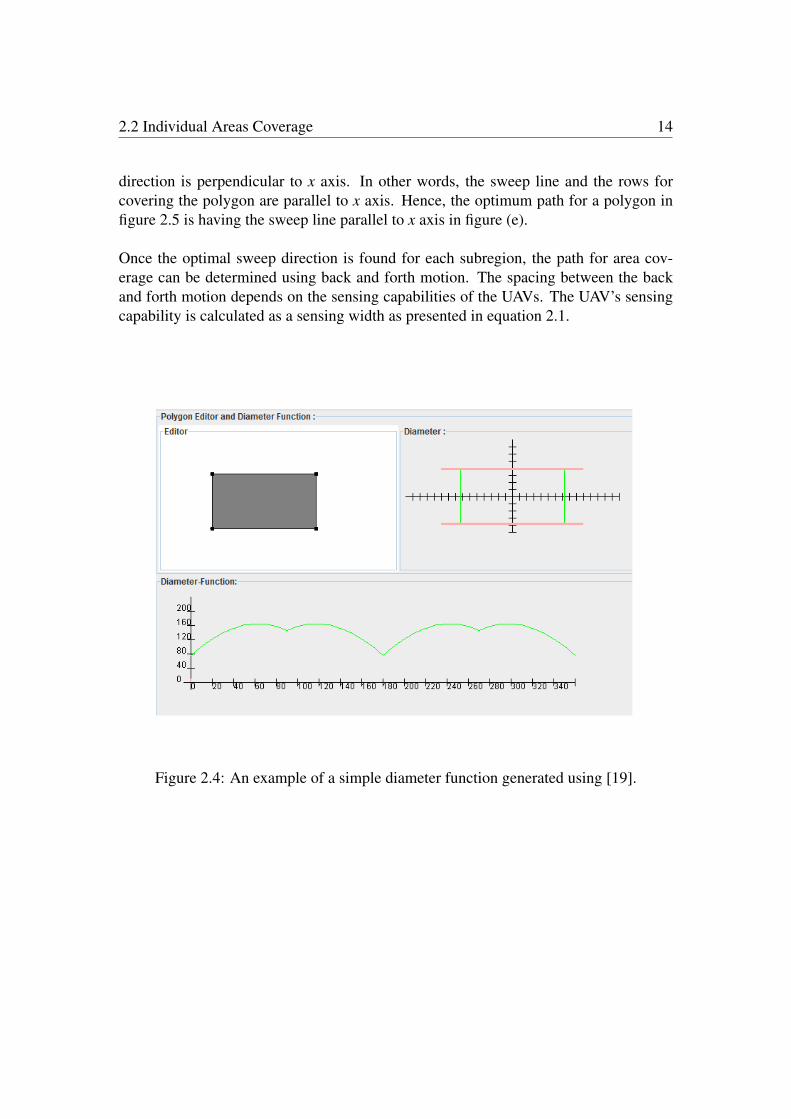
The optimal sweep direction can be determined from the minimum altitude of the poly-gon or the minimum diameter function. A diameter function d(θ) describes the heightof the polygon along the sweep direction. For a given angle θ , the diameter of a poly-gon is determined by rotating the polygon by −θ and measuring the height differencebetween its highest and lowest point [17]. The length of a diameter function can befound by considering the height of the polygon as it rolls along a flat surface. Figure 2.4shows an example of a diameter function of a rectangle generated using [19].
Figure 2.5 shows the diameter function of a polygon by rotating the figure counter-clockwise and finding its height. The angle that gives minimum diameter is a positionof the polygon for finding sweep direction. In the figure, the rotation of the polygon thatgives maximum diameter is shown in (d) and minimum diameter is shown in (e). Thesweeping path for covering the region has the least number of turns when the sweep
2.2 Individual Areas Coverage 14
direction is perpendicular to x axis. In other words, the sweep line and the rows forcovering the polygon are parallel to x axis. Hence, the optimum path for a polygon infigure 2.5 is having the sweep line parallel to x axis in figure (e).
Once the optimal sweep direction is found for each subregion, the path for area cov-erage can be determined using back and forth motion. The spacing between the backand forth motion depends on the sensing capabilities of the UAVs. The UAV’s sensingcapability is calculated as a sensing width as presented in equation 2.1.
Figure 2.4: An example of a simple diameter function generated using [19].

2.2 Individual Areas Coverage 15
Figure 2.5: Diameter of a polygon rotated counterclockwise. (a) 0 degree (b) 40 degree(c) 80 degree (d) maximum diameter at 289 degree (e) minimum diameter at 347 degree[19].

Chapter 3
Geometry-Based Area Decomposition
This chapter presents a proposed algorithm for area decomposition and algorithms forindividual areas coverage. The algorithms are aiming to minimize coverage time spend-ing on the areas by decreasing the number of turns in area coverage, and to minimizearea coverage redundancy. It is expected to reduce energy consumption and hoveringdistance.
As area decomposition algorithm presented in section 2.1.2 does not concern about theshape of the partitioned region, the resultant minimum diameter function is not optimal.The shape of the partitioned region should be considered in area decomposition becauseit relates to the number of turns when performing area coverage. Also with the locationof a base station, it should be considered because it relates to area coverage route andredundancy. Therefore, the decomposition algorithm should concern both shapes of thepartitioned regions and location of a base station concurrently.
The proposed area decomposition algorithm in this section concerns with area require-ment, location of a base station, and geometry of a polygon which affects shapes ofthe partitioned regions. The algorithm uses the area requirement to assign the size of asubregion. It makes use of the location of a base station to minimize route redundancyby determining the route that starts and ends at the base station without overlappingthe already visited region. It also considers geometry of a polygon to give partitionedregions with smaller minimum diameter functions, in order to decrease the number ofturns and increase the distance of straight paths.
The geometry-based area decomposition algorithm is presented in section 3.1. An anal-ysis of the algorithm is presented in section 3.2. Section 3.3 presents routes that giveless area coverage redundancy. Section 3.4 presents discussion and comparison of theresults from non-communicative area coverage and the proposed algorithms.
16

3.1 Decomposition Algorithm 17
3.1 Decomposition Algorithm
The algorithm aims to partition the region of interest such that an individual agent per-forms area coverage task in the subregion with less number of turns comparing to whenit performs in the subregion from section 2.2. The algorithm starts with examining thegeometry of a polygon P to find the longest side of the polygon, and then performspolygon decomposition.
As summarized in Algorithm 2, the algorithm requires that a line segment L dividingthe polygon P into two smaller polygons is parallel to the longest side of the polygonP. There are two cases for the decomposition. One is when the longest side is next tothe side of a base station, and another is when it is not. In the first case, the area de-composition is simple. The line segment L that divides the region of interest is parallelto the longest side. It moves toward or away from the longest side to vary the area of asubregion. In the second case, two line segments are used to divide the region. One isthe line segment parallel to the longest side and another one is the line segment parallelto the side adjacent to the side of a base station. The reasons behind these two line seg-ments are that the agent has more straight path when sweeping along the longest side,and it can start and end at the base station.
For the area partition of n agents, the algorithm has to perform n− 1 times for n sub-regions. The number of vertices of a polygon is denoted by parameter m. The verticesof polygon P in the algorithm are W (P) = Wi where i = 1, ...,m. In the first case ofdecomposition, a line segment that divides the polygon P into two convex pieces isL = (Ls,Le). The segment is oriented from Ls to Le. In the second case, a line segmentL1 is parallel to the side next to the side of a base station and a segment L2 is parallel tothe longest side of polygon P. An area requirement or desired area of each subregion isdenoted by AreaRequired.
Figure 3.1 illustrates the steps for dividing the polygon P in the second case wherethe longest side is not adjacent to the side of a base station. In this example, the polygonP is divided into three polygons with equal areas. Hence, the AreaRequired is 1
3 of areaof the polygon P. Figure (a) shows a polygon P with five vertices (m = 5). Its longestside Long is (W4,W5). Figure (b) shows line segments L1 and L2 that are parallel to sidesof the polygon P. In the figure, an area of a divided polygon P1(W1,Ls, its,Le,W4,W5)is smaller than the AreaRequired. Figure (c) shows an interpolation of the line segmentL2 that makes an area of the polygon P1 equal to the AreaRequired. Figure (d) showsthe complete polygon area decomposition where the polygon P is divided equally intothree polygons.

3.1 Decomposition Algorithm 18
Figure 3.1: Polygon area decomposition using geometry-based algorithm. The figureshows steps for dividing a polygon into three smaller polygons with equal areas.
3.1 Decomposition Algorithm 19
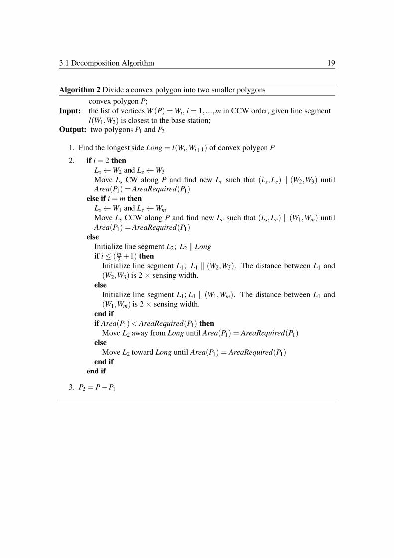
Algorithm 2 Divide a convex polygon into two smaller polygons
Input:convex polygon P;the list of vertices W (P) =Wi, i = 1, ...,m in CCW order, given line segmentl(W1,W2) is closest to the base station;
Output: two polygons P1 and P2
1. Find the longest side Long = l(Wi,Wi+1) of convex polygon P
2. if i = 2 thenLs←W2 and Le←W3Move Ls CW along P and find new Le such that (Ls,Le) ‖ (W2,W3) untilArea(P1) = AreaRequired(P1)
else if i = m thenLs←W1 and Le←WmMove Ls CCW along P and find new Le such that (Ls,Le) ‖ (W1,Wm) untilArea(P1) = AreaRequired(P1)
elseInitialize line segment L2; L2 ‖ Longif i≤ (m
2 +1) thenInitialize line segment L1; L1 ‖ (W2,W3). The distance between L1 and(W2,W3) is 2 × sensing width.
elseInitialize line segment L1; L1 ‖ (W1,Wm). The distance between L1 and(W1,Wm) is 2 × sensing width.
end ifif Area(P1)< AreaRequired(P1) then
Move L2 away from Long until Area(P1) = AreaRequired(P1)else
Move L2 toward Long until Area(P1) = AreaRequired(P1)end if
end if
3. P2 = P−P1

3.2 Algorithm Analysis 20
3.2 Algorithm Analysis
This section analyzes the geometry-based area decomposition algorithm whether it de-creases the number of turns in area coverage for any shape of convex polygons. Fromthe algorithm, there are two cases to consider. One is when the longest side of the regionof interest is next to the side of a base station, and another is when it is not, as shown infigure 3.2.
Figure 3.2: Regions of interest with different side of the longest side L.
Since an agent sweeps back and forth to perform area coverage, the number of turnsrelates to the number of rows it has to cover. Figure 3.3 shows partitioned regions fromthe polygons in figure 3.2. Figure (a) shows the first case of the decomposition. Thenumber of turns is determined from
number of turns = 2(d1
sensingwidth−1) (3.1)
where d1 is a minimum diameter function of the partitioned region and
number of rows =d1
sensingwidth. (3.2)
Figure (b) shows the decomposition where the subregion gives a better coverage pathwhen assigning it with different sweep directions. The diameter function consideredin this case is from the region connected to the longest side, since the region varies

3.2 Algorithm Analysis 21
Figure 3.3: The regions with different longest side are partitioned differently .
according to the area required. The number of turns in this subregion is determinedfrom
number of turns = 2(d2
sensingwidth−1)+2
= 2(d2
sensingwidth) (3.3)
where d2 is a minimum diameter function of the region connected to the longest side.
However, the number of turns in this case valid only on the condition that the num-ber of rows or d2
sensingwidth is an even number. Otherwise, it results in two additionalnumber of turns and route redundancy.
The diameter function is determined from [17] and sensing width is determined us-ing equation 2.1. If the UAVs are homogeneous, the sensing widths are the same. Thenumber of turns varies upon the size of the diameter function.
Figure 3.4 presents diameter functions of partitioned regions with equal area. The sub-region in figure (a) is from an algorithm presented in section 2.1.2. The subregion infigure (b) is from the proposed algorithm. The number of turns in both figure (a) and(b) are calculated using equation 3.1.
From the figure, the diameter function of a subregion in figure (b) is shorter than infigure (a). This is due to the constraint in the proposed decomposition algorithm that

3.2 Algorithm Analysis 22
Figure 3.4: Diameter functions of subregions with equal area but are partitioned usingdifferent algorithm.
a partitioning line segment must be parallel to a longest side L. Accordingly, in anypartitioned regions
d2 ≤ d1 (3.4)
where d2 is the diameter function of a subregion from the proposed algorithm and d1 isthe diameter function of a subregion from section 2.1.2 algorithm.
The number of turns is an integer. From the numerical rounding, the number of turnsof a subregion from the proposed algorithm is less than from algorithm presented insection 2.1.2 if
d1−d2 >sensingwidth
2. (3.5)
If the longest side of a polygon is not adjacent to the side of a base station, the numberof turns of a subregion from the proposed algorithm is calculated using equation 3.3 andthe subregion from section 2.1.2 is calculated using equation 3.1. Figure 3.5 shows thepartitioned regions from both algorithms and their diameter functions. The partitionedregions have the same area, but with different diameter function. According to equation3.1 and 3.3, the number of turns is improved if
d1−d2 > 2× sensingwidth. (3.6)

3.2 Algorithm Analysis 23
Figure 3.5: Diameter functions of subregions with equal area but are partitioned usingdifferent algorithm.
Figure 3.6: Diameter function of a partitioned region from 2.1.2 is the shortest in figure(a). Figure (b) is the partitioned region from proposed algorithm with equal area to (a).
Consider partitioned regions in figure 3.6 where both the regions have the same area. Infigure (a), the diameter function d1 is the shortest when using area decomposition pre-sented in section 2.1.2. Figure (b) is the partitioned region from the proposed algorithmwith the same area as in (a).
Area = d1l = d2L+(l−d2)(2s)
d1 =d2L+2ls+2d2s
l(3.7)
where s is the sensing width.

3.3 Area Coverage Redundancy 24
Substitute eq. 3.7 in eq. 3.6 gives
L− l > 2× sensingwidth. (3.8)
Hence, in the second case, the number of turns is improved if the longest side is longerthan the side adjacent to the base station twice the sensor width. If not, the region shouldbe decomposed as if the longest side is l and follow the first case.
3.3 Area Coverage Redundancy
Area coverage redundancy is overlapped areas when the agents perform area coveragetask, or covered areas that are not in a region of interest. The redundancy does not giveproductive surveillance. It wastes both time and energy consumption.
In individual areas coverage algorithm presented in section 2.2, the algorithm applies anoptimal line-sweep-based decomposition [17] which gives area coverage in each sub-region with minimum number of turns. However, the algorithm does not concern overarea coverage redundancy. The redundancy from overlapped areas usually occurs whenan agent are obliged to start and end at the same base station. When an agent completedits area coverage task, it returns to the base station. Its return route repeats the alreadyvisited region and causes overlapped area if the final area coverage position is not at thebase station.
The overlapped area is determined from the distance between the agent’s final areacoverage position and the base station. This final area coverage position depends onthe start position, the size of the diameter function, and route generation of the UAV asshown in figure 3.7, 3.8, and 3.9 respectively.
In figure 3.7, the final area coverage positions are different as the agent starts its routeat different location. There are route overlaps in both figure (a) and (b). The overlapin figure (b) is less than in (a) since the final position in (b) is closer to the base stationthan in (a).
The size of a subregion’s minimum diameter function should also be concerned whendecomposing a region of interest. It defines the number of rows an agent has to coverwhen performing area coverage. The number of rows is determined from equation 3.2.It affects the agent’s final area coverage position and hence route redundancy. Whendecomposing the region, the size of minimum diameter function should be
2n× sensingwidth (3.9)

3.3 Area Coverage Redundancy 25
Figure 3.7: Route comparison of the same polygon but with different start position.
where n = 1,2, ...,n. The sensing width defines the distance between back and forthmotion which is determined from equation 2.1. The diameter function of a subregionaccording to equation 3.9 allows the agents to start and end the area coverage task at thesame base station and eliminates the area coverage redundancy.
Figure 3.8 shows an example of a polygon with different minimum diameter func-tion of partitioned regions. In figure (a), the diameter function is equal to five sensingwidth. The final area coverage position of a UAV is not on the side closest to a basestation. Hence, the return route will overlap an already covered area. In figure (b), thesubregion’s minimum diameter function is according to equation 3.9. The area coverageroute sweeps the subregion completely without route overlap. The entire route resultsin productive area coverage.
When decomposing the region considering this criterion, the area of the partitionedregion might contradict the AreaRequired. The area of the partitioned region can beless than the AreaRequired. However, it should not be more than the AreaRequiredsince it might exceed the agent’s capability. This criterion also affects the area of otherpartitioned regions, hence it should be considered concurrently when performing area

3.4 Discussion and Results 26
Figure 3.8: Different width of partitioned regions result in different overlapped area.
decomposition algorithms.
When decomposing a region, there is one last subregion that may not fit into thepresented scheme, i.e. no side parallel to the partitioning line segment. The route forthis subregion is determined from the direction of minimum diameter function and theposition of the base station. To remove route overlap, both start and end positions of theroute should be close to the base station or the return route should be part of the areacoverage path.
Figure 3.9 shows an example of possible route generation. The routes in both figure(a) and (b) are generated toward the direction of minimum diameter function for min-imum number of turns. However, a route overlap is also concerned in figure (b). Theroute in figure (b) allows an agent to start and end at the base station without overlap.
3.4 Discussion and Results
There are various factors that influence the performance of non-communicative areacoverage. The ones already been examined in this thesis are sensor range, area de-composition, and individual areas coverage algorithm. The efficiency of the UAVs isdepending on the design or purpose of each UAV which can be various in speeds, sta-bility, battery lifetime, and etc. Unpredictable factors such as environment of a region
3.4 Discussion and Results 27
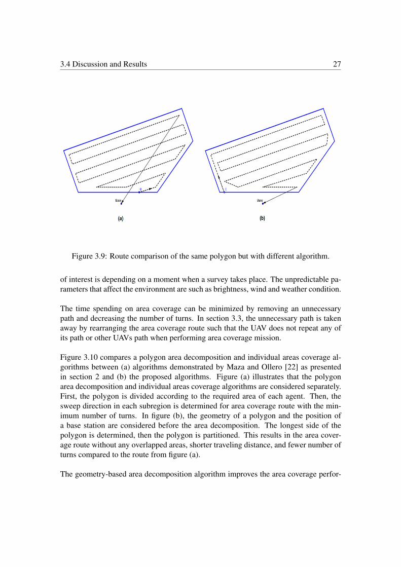
Figure 3.9: Route comparison of the same polygon but with different algorithm.
of interest is depending on a moment when a survey takes place. The unpredictable pa-rameters that affect the environment are such as brightness, wind and weather condition.
The time spending on area coverage can be minimized by removing an unnecessarypath and decreasing the number of turns. In section 3.3, the unnecessary path is takenaway by rearranging the area coverage route such that the UAV does not repeat any ofits path or other UAVs path when performing area coverage mission.
Figure 3.10 compares a polygon area decomposition and individual areas coverage al-gorithms between (a) algorithms demonstrated by Maza and Ollero [22] as presentedin section 2 and (b) the proposed algorithms. Figure (a) illustrates that the polygonarea decomposition and individual areas coverage algorithms are considered separately.First, the polygon is divided according to the required area of each agent. Then, thesweep direction in each subregion is determined for area coverage route with the min-imum number of turns. In figure (b), the geometry of a polygon and the position ofa base station are considered before the area decomposition. The longest side of thepolygon is determined, then the polygon is partitioned. This results in the area cover-age route without any overlapped areas, shorter traveling distance, and fewer number ofturns compared to the route from figure (a).
The geometry-based area decomposition algorithm improves the area coverage perfor-

3.4 Discussion and Results 28
mance most when a polygon P has one side apparently longer than the others. With thispolygon, the UAVs can sweep along the longest side having longer distance on straightpaths and less number of turns.
Figure 3.10: Area decomposition and route generation of a polygon using differentalgorithms.

Chapter 4
Communicative Area Coverage
Communications plays a much more important part in the overall operation of a UAVthan it does for manned aircraft because the men-in-the-loop are on the ground [7].Communications gives more robust area coverage algorithm. It allows a base station toknow the location and situation of each agent. The base station is able to obtain imagesfrom the observed area in near real time using wireless communication system. This ishelpful for the base station, especially if the data is critical and time-sensitive. More-over, it can command the agents to go to specific locations or return to the base station.
Given that the region of interest is in a disaster area or there exists no networking in-frastructure, mobile ad hoc networks (MANETs) offer a way to maintain connectivitybetween the agents. The MANETs communications are performed over radio and donot require any infrastructure. They are very flexible and suitable for several types ofapplications as they allow the establishment of temporary communication without anypre-installed infrastructure [12].
With MANETs, the UAVs nodes can dynamically located into arbitrary and temporarynetwork topologies. The networks provide the most mobile and least purpose-specifictype of wireless ad hoc networks [26]. They are meant to provide an immediate con-nectivity in any situation. However, as it uses wireless communication as a medium,characteristics such as high bit error rate, path loss or signal strength attenuation, multi-path fading, interference, delay spread, and penetration loss should be considered [23],[24].
The purpose of this chapter is to place a certain number of nodes such that a regionof interest is completely covered and all the nodes and a base station can communicate.The node placement can be classified into static positioning and dynamic positioningscheme. In static positioning, the placement of the nodes is determined by the basestation before a task begins. These UAV nodes will go to the predefined locations when
29

4.1 Static Positioning of Nodes 30
the task begins. The placement calculation is based on the region of interest and sensingrange of the nodes.
In dynamic positioning, the placement is determined by each node during the task. Theplacement calculation for each node is based on current locations of the node and itsneighbors, communication range, sensing range and the region of interest. In this dy-namic scheme, the nodes find their new locations autonomously and they can repositionthemselves when there is one or more missing nodes in the region.
The UAV nodes are equipped with a low-power Global Positioning System (GPS) re-ceiver to obtain their positions. The UAVs use GPS to navigate them to the predefinedpositions in static positioning, and to determine their positions and the positions of theirneighbors in autonomously dynamic positioning.
In this thesis, all the nodes are assumed to have the same sensing range and maxi-mum transmission range. The transmission range is at least twice the size of the sensingrange. Each of the nodes has distinct identity. Uniform node distribution can be appliedto spread the UAVs over a region of interest evenly and achieve maximum coverage.The complete coverage of the nodes allows the base station to obtain the whole imageof the region of interest and lets all the agents to stay connected.
Section 4.1 presents static positioning of the nodes and minimum number of nodesrequired to completely cover the region of interest. Section 4.2 presents three methodsfor dynamic repositioning; DSSA, VDDA, and the centroid-based scheme. Simulationresults and analysis when applying the algorithms to a given situation is presented insection 4.3.
4.1 Static Positioning of Nodes
When the environment is sufficiently known, the positions of the nodes can be prede-termined. Different clustering shapes could be used to subdivide a region of interestand determine locations of the nodes. The region is subdivided using identical clus-tering cells and with no overlaps between the cells. The popular clustering shapes forthe nodes deployment are circle, square, and hexagon. The circle shape is the "mostnatural" cluster because it coincides with the shape of the radio transmission range [27].However, these clusters have to be overlapped to completely cover the region of interest.There is no hint on the circles how much they should overlap. Hence, it is more com-plicated than the other clustering shapes in determining uniform locations of the nodesthat can completely cover the region of interest.

4.1 Static Positioning of Nodes 31
An ideal shape for clustering is the one that tessellating cells are adjacent to each otherwithout any holes and overlapping areas. The shapes that have this property are triangle,square, and hexagon. Among these shapes, hexagon is the best clustering shape becauseit is the largest polygon (in terms of number of sides) that has this property [27] and thedistances between the node and all the adjacent neighbors are equal.
Figure 4.1 illustrates different clustering shapes for node deployment. In figure (a), thecircle cells could not cover the entire network without overlap. Figure (b) shows squareclusters where there is no uncovered area, but the distance between two adjoining nodesand diagonal nodes are not equal. Figure (c) demonstrates hexagonal clustering nodeswhere the distances between the node and its neighbors are the same in all direction.
Figure 4.1: The clustering shapes of circle (a), square (b), and hexagon (c).
4.1.1 Minimum number of nodes
The number of agents required to completely cover the region of interest depends onthe sensing range and the shape of the region. The distance between the agent and itsadjacent neighbors or between the agent and its adjacent boundary must not exceed thesensing range so that the entire region is covered. There is no general solution to find theminimum number of agents required to completely cover the region. The regions withequal area might require different number of agents, if the shapes of the two regions

4.1 Static Positioning of Nodes 32
were different.
To uniformly place the nodes in the region, regular hexagonal tiling could be applied.The nodes are placed at the center of the hexagons. The size of the hexagons corre-sponds to the node’s maximum sensing range to reduce overlapped sensing regions.The hexagons are considered in node positioning if their centers lie inside the region ofinterest. These hexagons give approximate number and positions of node positioning.
Figure 4.2 demonstrates the uniform distribution of the nodes that lie inside the regionof interest. Figure (a) shows the hexagonal tiling and the positions of the nodes. Figure(b) shows the sensing regions according to the node positions in figure (a). The numberof agents in this figure is 17, however, the region is not entirely covered.
Figure 4.2: Regular hexagonal tiling inside the region of interest (a) and the nodessensing regions (b).

4.1 Static Positioning of Nodes 33
Figure 4.3: Node locations and their sensing regions.
Additional nodes are required to cover the whole region as shown in figure 4.3. In thefigure, the number of agents in the region is 23. The number of the nodes is not mini-mized since additional nodes give large redundant covered regions. The nodes could berelocated to reduce the number needed.
Figure 4.4: Regular hexagonal tiling (a) and hexagonal tiling adjusted according to thewidth of the region (b).
The nodes relocation can be done by changing the dimension of the hexagonal tile. Fig-ure 4.4 illustrates the first layer of the hexagonal tiling. In figure (a), the nodes arelocated according to regular hexagonal tiling where all the sides are equal. There is

4.1 Static Positioning of Nodes 34
uncovered region in this first layer figure since the width of the hexagonal tiles and theregion are not proportional. In figure (b), the width of the tiles is adjusted according tothe size of the region. The width is smaller but the vertical sides are longer. The nodescover the whole layer in this figure.
To adjust the width of the hexagon, the number of the tiles required in the first layeris determined from
n = d wr
r√
3e (4.1)
where r is the maximum sensing range and wr is the width of a region when y= r. Then,as shown in figure 4.5, find y = h that makes
h2=
√r2− d
2
2(4.2)
where d is the width of each hexagonal tile and d < r√
3. d is determined from the ratioof the width of the region wh at y = h and the number of required tiles n:
d =wh
n. (4.3)
Figure 4.5: Hexagon and the length of each side. Figure (a) is a regular hexagon. Figure(b) is the hexagon adjusted according to the width of the region.
4.1 Static Positioning of Nodes 35
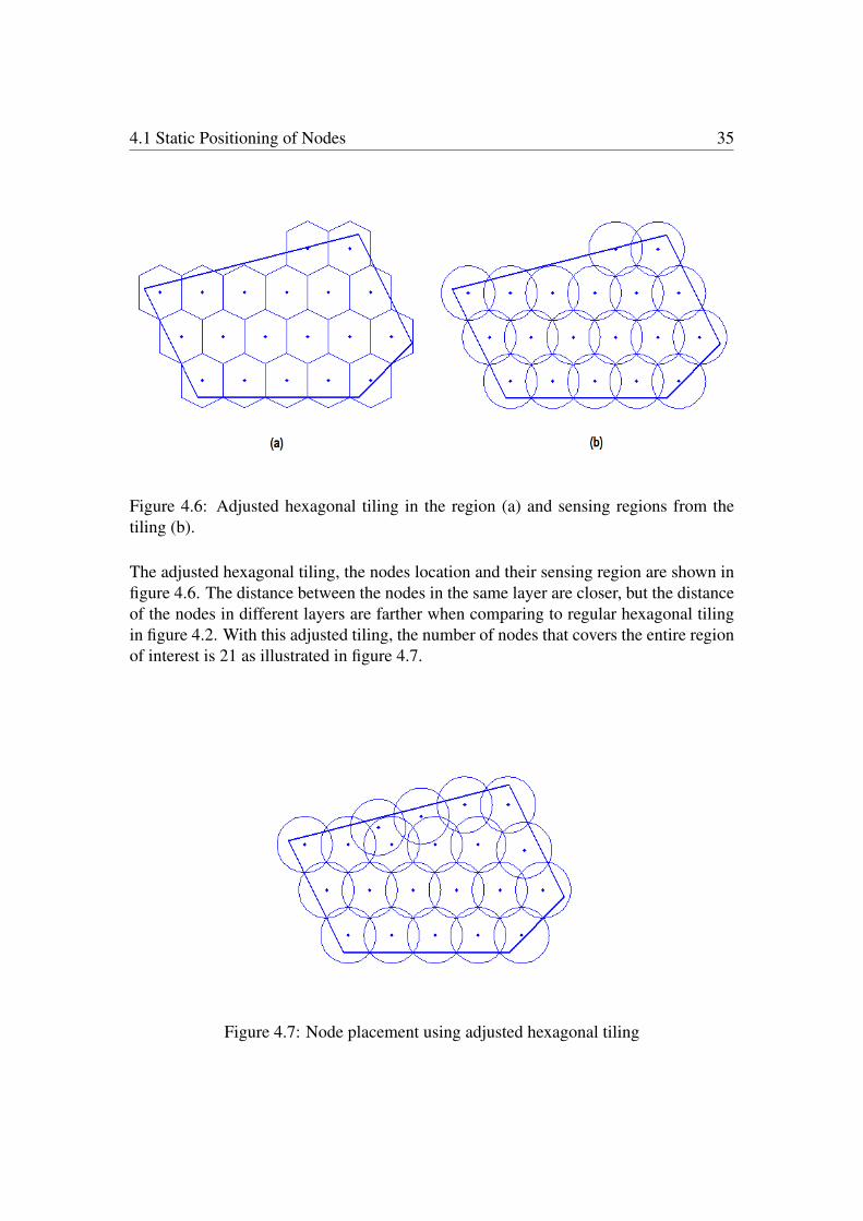
Figure 4.6: Adjusted hexagonal tiling in the region (a) and sensing regions from thetiling (b).
The adjusted hexagonal tiling, the nodes location and their sensing region are shown infigure 4.6. The distance between the nodes in the same layer are closer, but the distanceof the nodes in different layers are farther when comparing to regular hexagonal tilingin figure 4.2. With this adjusted tiling, the number of nodes that covers the entire regionof interest is 21 as illustrated in figure 4.7.
Figure 4.7: Node placement using adjusted hexagonal tiling
4.2 Dynamic Repositioning of Nodes 36
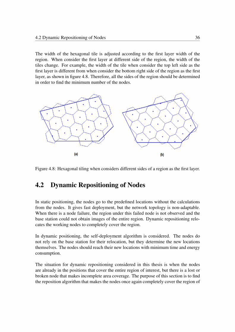
The width of the hexagonal tile is adjusted according to the first layer width of theregion. When consider the first layer at different side of the region, the width of thetiles change. For example, the width of the tile when consider the top left side as thefirst layer is different from when consider the bottom right side of the region as the firstlayer, as shown in figure 4.8. Therefore, all the sides of the region should be determinedin order to find the minimum number of the nodes.
Figure 4.8: Hexagonal tiling when considers different sides of a region as the first layer.
4.2 Dynamic Repositioning of Nodes
In static positioning, the nodes go to the predefined locations without the calculationsfrom the nodes. It gives fast deployment, but the network topology is non-adaptable.When there is a node failure, the region under this failed node is not observed and thebase station could not obtain images of the entire region. Dynamic repositioning relo-cates the working nodes to completely cover the region.
In dynamic positioning, the self-deployment algorithm is considered. The nodes donot rely on the base station for their relocation, but they determine the new locationsthemselves. The nodes should reach their new locations with minimum time and energyconsumption.
The situation for dynamic repositioning considered in this thesis is when the nodesare already in the positions that cover the entire region of interest, but there is a lost orbroken node that makes incomplete area coverage. The purpose of this section is to findthe reposition algorithm that makes the nodes once again completely cover the region of

4.2 Dynamic Repositioning of Nodes 37
interest. The nodes should be able to reposition themselves when they sense that theirneighboring node is lost or broken down. Repositioning compensates the lost in cov-erage and/or network connectivity of a missing node. It is necessary in communicativesurveillance task, especially in a situation where the number of mobile agent changeswith time; e.g. due to forest fire, hostile attacks, or malfunctions.
There are many algorithms for the nodes dynamic repositioning as presented in [28].The nodes are repositioned based on the quality of their performance metrics such asthe data rate, sensing range, path length in terms of the number of hops from a sensornode to the base station, etc. This thesis only considers repositioning when there is aregion out of the nodes’ sensing ranges.
The algorithms presented in this section are DSSA [13], VDDA [14], and the centroid-based scheme [20]. The DSSA algorithm which applies the concept of force in physicsfor node positioning is presented in section 4.2.1. Section 4.2.2 presents the VDDA al-gorithm where local Voronoi diagram is used to calculate the effective area of the nodes.Section 4.2.3 presents the centroid-based scheme which used Voronoi diagram and cen-troid of the polygon for node relocation.
4.2.1 Distributed Self-Spreading Algorithm (DSSA)
This algorithm is introduced by Heo and Varshney [13]. It is the peer-to-peer algorithminspired by the equilibrium of molecules. The algorithm applies inter-nuclear repulsionand attractions between molecules. If the nodes are located too close to each other, thecoverage gaining from these nodes is not high. On the contrary, if the nodes are lo-cated too far from each other, the coverage regions may not overlap and the region isnot entirely covered. The optimal spacing between the nodes can be determined from aprocess similar to the equilibrium of molecules.
The algorithm begins with a specified number of nodes scattered randomly in a givenregion. These nodes have communication range and sensing range to sense an environ-ment within its sensing region. Any pair of nodes within their communication range areconsidered neighborhood and can communicate with each other. Within neighborhood,locations of the nodes can be obtained and the sensed data can be received and transmit-ted. Algorithm 3 [14] shows the pseudocode of the algorithm executed at each node i.The algorithm contains four parts.

4.2 Dynamic Repositioning of Nodes 38
Algorithm 3 Distributed Self Spreading Algorithm [14]
1. Initialization
initial node locations p0;sensing range sR;communication range cR;calculate local density D;calculate expected density µ;
While (Not(Oscillation occured OR In a region of stability))
2. Partial Force Calculation
calculate partial force f i, jn (µ,D,cR, pn);
update temporary position pin+1;
3. Oscillation Check
If (|pin−1− pi
n+1|< threshold1)
Increase oscillation count by 1;If (oscillation count < oscillation limit)
Update next location to the temporary position;Update local density D;ElseMove to the centroid of oscillating points;Update local density D;Stop node i’s movement;ElseUpdate next location to the temporary position;Update local density D;
4. Stability Check
If (|pin+1− pi
n|< threshold2)
Increase stability count by 1;If (stability count < stability limit);
Go to while loop;
ElseStop node i’s movement;
Else
Go to while loop;
4.2 Dynamic Repositioning of Nodes 39
1. Initialization: First, each node specifies the given communication range (cR) andsensor range (sR). The initial node locations (p0) are specified in terms of a vectorthat contains the longitude component and the latitude component of each nodelocation. Then expected density which is a rough estimation of the desired densityis calculated from
µ(cR) =N ·π · cR2
A(4.4)
where N is the number of nodes, cR is the communication range, and A is the areaof the region of interest. The expected density µ is the average number of nodesrequired to uniformly cover the entire area. The number of nodes within a node’scommunication range is local density (D). D0 is an initial local density. Thesedensities will be used when decisions regarding positions of nodes are made.
2. Partial Force Calculation: The algorithm applies the concept of force to definethe movement of nodes during node placement method. The concept dependsnot only on the distance between a node and its neighboring nodes within itscommunication range, but also on the current local density. The force resultingfrom high local density is greater than the force resulting from low local density.Also, the force from a closer neighbor is greater than the force from a fartherneighbor. The force function is defined to satisfy the following conditions:
(a) Inverse relation: f (d1) ≥ f (d2), when d1 ≤ d2 , where d1 and d2 are nodeseparations from the origin.
(b) Upper bound: f (0+) = fmax.
(c) Lower bound: f (d) = 0, where d > cR, d is the node separation and cR isthe communication range of each node.
Condition (a) is the same as in physics that follow Coulomb’s law. Condition(b) and (c) are included to incorporate the notion of locality. They are a limitingfunction applied to a node’s neighborhood.
The partial force on node i from its neighboring node j at time step n is calculatedto be a repulsive force as
f i, jn =
Din
µ2 (cR−|pin− p j
n|)p j
n− pin
|pin− p j
n|(4.5)
where
cR stands for communication range;

4.2 Dynamic Repositioning of Nodes 40
pin stands for the location of ith node at time step n;
Din stands for the local density of ith node at time step n.
From equation 4.5, the distance between a node and its neighboring nodes affectsthe partial force inversely. Closely located nodes impose larger partial forceswhile sparsely located nodes induce smaller partial forces. The magnitude of thepartial force exerted by a pair of nodes on each other are the same but with thedirections opposite to each other. The ratio of the local density (D) and the squareof the expected density (µ) at each node define the density factor ( D
µ2 ). This den-sity factor is small in sparse regions and is large in dense regions.
Each node can decide its next movement, after calculating the partial forces forall nodes at time step n. The node’s movement is decided from the collection offorces due to the nodes in its neighborhood. After the node moves to new posi-tion at time step n+1, it updates the local information at this position. The localinformation is collected from the nodes that are within the communication rangeand will be used for the calculation of the local density at each node. Again, thepartial force is calculated and the next movement is generated.
3. Oscillation Check: The nodes will stop their movements from two criteria. Thefirst criterion is when a node moves back and forth between almost the same loca-tions many times. This node is regarded as in the oscillation state. To determinewhether the oscillation is going on or not, the history of a node’s movement is ex-amined. If the number of node’s oscillations (Ocount) is over the oscillation limit(Olim), the node’s movement is stopped at the center of gravity of the oscillatingpoints.
4. Stability Check: The second criterion for stopping a node’s movement is when thenode moves less than threshold2 for the time duration Stability_limit(Slim). Thisis due to three reasons.
• The node has reached its stable state
• Fuel exhaustion
• Broken mobile units
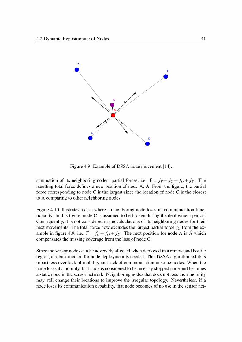
Figure 4.9 illustrates an example of a node movement when applies DSSA algorithmto node A. Nodes B, C, D, E are neighboring nodes. They are located within node A’scommunication range. The partial forces fB, fC, fD, and fE of the neighboring nodes arecalculated using equation 4.5. The total force F on node A is obtained from the vectors
4.2 Dynamic Repositioning of Nodes 41
Figure 4.9: Example of DSSA node movement [14].
summation of its neighboring nodes’ partial forces, i.e., F = fB + fC + fD + fE . Theresulting total force defines a new position of node A; Á. From the figure, the partialforce corresponding to node C is the largest since the location of node C is the closestto A comparing to other neighboring nodes.
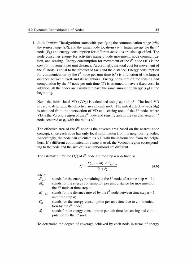
Figure 4.10 illustrates a case where a neighboring node loses its communication func-tionality. In this figure, node C is assumed to be broken during the deployment period.Consequently, it is not considered in the calculations of its neighboring nodes for theirnext movements. The total force now excludes the largest partial force fC from the ex-ample in figure 4.9, i.e., F = fB + fD + fE . The next position for node A is Á whichcompensates the missing coverage from the loss of node C.
Since the sensor nodes can be adversely affected when deployed in a remote and hostileregion, a robust method for node deployment is needed. This DSSA algorithm exhibitsrobustness over lack of mobility and lack of communication in some nodes. When thenode loses its mobility, that node is considered to be an early stopped node and becomesa static node in the sensor network. Neighboring nodes that does not lose their mobilitymay still change their locations to improve the irregular topology. Nevertheless, if anode loses its communication capability, that node becomes of no use in the sensor net-

4.2 Dynamic Repositioning of Nodes 42
Figure 4.10: Example of DSSA node movement with a failed node [14].
work. Its neighboring nodes have to rearrange the locations to cover the region insteadof the broken node.
4.2.2 VD-Based Deployment Algorithm (VDDA)
Voronoi diagram is one of the most fundamental data structures in computational geom-etry. Many researchers have demonstrated the importance and usefulness of the Voronoidiagram in a wide variety of fields including mathematics, computational geometry, bi-ology, chemistry, geography, communications, and coding theory [3].
Figure 4.11 shows an example of a Voronoi diagram. Given a number of points inthe region of interest, Voronoi diagram can be used to decompose these points intonon-overlapping Voronoi cells (Voronoi region). The cells are divided according to thenearest-neighbor rule. Each given point in the Voronoi cell is associated with the cellsof points in the region of interest that are closest to it. These given points and theircorresponding Voronoi cells can be applied to the node placement problem by defining

4.2 Dynamic Repositioning of Nodes 43
Figure 4.11: Voronoi diagram
the points as the nodes and the Voronoi cells as the communication ranges. Hence, adeployment algorithm for communication can be developed using the notion of Voronoiregions.
This VD-based deployment algorithm (VDDA) is from [14]. The goal of this algorithmis to have the Voronoi cell corresponding to the node’s sensing range. The Voronoi cellthat matches with a node’s sensing range at a certain time instance is considered to bethe desired solution in terms of coverage. If the difference between the node’s sens-ing range and the Voronoi cell corresponding to that node are not within the predefinedtolerance, the node is moved. It is moved until the sensing range and the Voronoi cellare aligned, then the nodal movement is stopped and the resulting solution is accepted.The algorithm from [14] for VD-based deployment is presented in Algorithm 4. Thisdistributed algorithm is executed at each node i. The algorithm comprises of two steps:initialization and finding the best energy-utilization point.

4.2 Dynamic Repositioning of Nodes 44
Algorithm 4 Voronoi Diagram based Deployment Algorithm [14]
1. Initialization
initial node locations p0;sensing range sR;communication range cR;initial energy E i
0;energy consumption rate Mi
0, Ci0, Si
0;calculate initial V D(p0,cR);calculate initial effective area Ai
0 from V D(p0,cR) and SensingArea(pi0,sR);
calculate initial estimated lifetime T i0 ;
calculate initial node utility U i0 = Ai
0×T i0 ;
While (Not(utility gain > a predefined threshold))
2. Find the maximal energy utilization point
Set the current solution as the last solution of previous step: U imax,n =U i
n−1
calculate V D(pn,cR)find the centroid of VD: V D1
{ search max. energy utilization point among points linearly spaced between pi and V D1
calculate effective area Ait,n from V D(pn,cR) and SensingArea(pi
t,n,sR)calculate energy consumption rate Mi
t,n, Cit,n, Si
t,n
calculate estimated lifetime T it,n
if U it,n >U i
max,n
U imax,n =U i
t,n
elsekeep searching
endupdate pi }
find the mean of maxVD and min VD: V D2
{ search max. energy utilization point among points linearly spaced between pi and V D2
calculate effective area Ait,n from V D(pn,cR) and SensingArea(pi
t,n,sR)calculate energy consumption rate Mi
t,n, Cit,n, Si
t,n
calculate estimated lifetime T it,n
if U it,n >U i
max,n
U imax,n =U i
t,n
elsekeep searching
end }
update pi
update U in =U i
max,n
update current energy E in
End of while loop
4.2 Dynamic Repositioning of Nodes 45
1. Initialization: The algorithm starts with specifying the communication range (cR),the sensor range (sR), and the initial node locations (p0). Initial energy for the ith
node (E i0) and energy consumption for different activities are also specified. The
node consumes energy for activities namely node movement, node communica-tion, and sensing. Energy consumption for movement of the ith node (Mi) is thecost for movement per unit distance. Accordingly, the total cost for movement ofthe ith node is equal to the product of (Mi) and the distance. Energy consumptionfor communication by the ith node per unit time (Ci) is a function of the largestdistance between itself and its neighbors. Energy consumption for sensing andcomputation by the ith node per unit time (Si) is assumed to have a fixed cost. Inaddition, all the nodes are assumed to have the same amount of energy (E0) at thebeginning.
Next, the initial local VD (V D0) is calculated using p0 and cR. The local VDis used to determine the effective area of each node. The initial effective area (A0)is obtained from the intersection of VD and sensing area of the ith node, whereVD is the Voronoi region of the ith node and sensing area is the circular area of ith
node centered at p0 with the radius sR.
The effective area of the ith node is the covered area based on the nearest nodeconcept, since each node has only local information from its neighboring nodes.Accordingly, the node can calculate its VD with the information from the neigh-bors. If a different communication range is used, the Voronoi region correspond-ing to the node and the size of its neighborhood are different.
The estimated lifetime (T in) of ith node at time step n is defined as
T in =
E in−1−Mi
n×din−1,n
Cin +Si
n(4.6)
whereE i
n−1 stands for the energy remaining at the ith node after time step n−1;Mi
n stands for the energy consumption per unit distance for movement ofthe ith node at time step n;
din−1,n stands for the distance moved by the ith node between time step n−1
and time step n;Ci
n stands for the energy consumption per unit time due to communica-tion by the ith node;
Sin stands for the energy consumption per unit time for sensing and com-
putation by the ith node.
To determine the degree of coverage achieved by each node in terms of energy

4.2 Dynamic Repositioning of Nodes 46
efficiency, a node utility metric is considered. The node utility metric (U) indi-cates how well the node is utilized to cover its effective area during the lifetime.Consequently, it is used to decide energy-efficient movements by each node. Thenode utility metric (U i
n) of the ith node at time step n is defined as
U in = Ai
n×T in (4.7)
whereAi
n represents the effective area covered by the ith node at time step n;T i
n represents the estimated lifetime of the ith node at time step n.
2. Finding the Best Energy-Utilization Point: The best energy-utilization point ofeach node is obtained by comparing utility gains that a node would achieve whenmoving to different possible node locations. A movement from the current loca-tion to different node locations may or may not reduce the communication cost,but it will cost energy consumption depending on the node destination.
In VDDA, the local VDs are used to reduce the search space from infinite num-ber when considering continuous coordinates. The local Voronoi region can beconsidered as the estimated or desired coverage by the local node due to the near-est neighbor relation of VDs. Since coverage area of a node is circular, movingthe node to the centroid of the Voronoi region would enhance the nodes coverageand/or uniformity. Another node location that can be used to guide the search isthe center of the Voronoi range. It is defined as the midpoint of the maximum andminimum along the x and y coordinates in the Voronoi region.
The local VDs reduce search space to several points linearly spaced. The searchspace starts from the current location to the centroid of the Voronoi region, andthen from the centroid to the center of the Voronoi range. In these searched points,the node utility metric is evaluated and the best action is determined. From thealgorithm, the node utility metric is iteratively calculated and compared to theprevious value. During the search process, only the best solution is kept. There-fore, a locally optimal solution is obtained after the search process.
Once the best energy-utilization point is found, actual movement of each nodeoccurs. The movement takes place only after the best solution is found in order tosave energy consumption.

4.2 Dynamic Repositioning of Nodes 47
4.2.3 The Centroid-based Scheme
This algorithm is from [20]. The algorithm uses the Voronoi diagram to determine theregion that the node has to cover. It uses centroid of a polygon to decide the nodes’ nextmovement. The algorithm is similar to VDDA that the nodes have to calculate theirVoronoi regions at the beginning of each round of nodes moving. However, it does notsearch for the maximum gain among the points linearly spaced between the current nodelocation and the centroid of Voronoi region. The node simply moves to the centriod ofthe region if it gives better local coverage.
The algorithm starts with initializing all the node locations and their sensing range andcommunication range. It then calculates the Voronoi region of a node using the nodelocation and its communication range. If the Voronoi region is fully covered by thenode’s sensing range, the node does not move at this round. The Voronoi region is fullycovered when all distances from the local Voronoi vertices to the nodes are less than thenode’s sensing range.
If the node’s sensing range does not fully cover the Voronoi region, the centroid of theVoronoi region is determined. The node checks whether the local coverage will increaseby its movement to the new location. If the node covers more Voronoi region at the newlocation, it will move; otherwise, it will stay at its current location. The algorithm issummarized as shown in Algorithm 5.

4.3 Simulation Results and Analysis 48
Algorithm 5 The Centroid Scheme
1. Initializationinitial node locations p0;sensing range sR;communication range cR;calculate initial V D(p0,cR);calculate all the distances between Voronoi vertices and node locations
D(V D, p0);
While (D(V D, p0) > sR))
2. Relocationcalculate centroid of the Voronoi region C(V D)
if (moving node to C(V D) increases local coverage)move the node to C(V D)update node location pncalculate V D(pn,cR)calculate D(V D, pn)
elsebreak
end
End of while loop
4.3 Simulation Results and Analysis
This chapter has presented the methods for nodes positioning both statically and dy-namically. Given a situation where a region of interest needs to be observed as long aspossible, a sufficient number of nodes have to spread over the region of interest. Theminimum number of nodes from section 4.1.1 is enough to completely cover the regionof interest, however, the coverage is not robust against potential vehicle failures.
An extra number of nodes is added to the region in case of potential node failure. Thenumber of nodes that completely cover the region of interest and robust against the fail-ure is shown in figure 4.12. The figure shows an example of predetermined positions of

4.3 Simulation Results and Analysis 49
the nodes when the sensing range is 80% of its maximum sensing range. In figure (a)the region is fully covered by the nodes. There is one missing node in figure (b).
Figure 4.12: Node placement where the sensing range is 80% of its maximum sensingrange. All the agents function properly in (a). In (b) there is one missing agent.
When there is one or more missing nodes, dynamic repositioning can be used to relocatethe nodes autonomously. In this thesis, the dynamic repositioning algorithms that areapplied to the situation are DSSA, VDDA, and the centroid scheme.
When applying DSSA algorithm to the situation, the nodes move according to the po-sitions of their neighbors. The neighbors of the missing node tend to move toward themissing node’s direction since there is no force exerting from that direction. Owing tothis, the nodes located near the boundary are also likely to move out of the region ofinterest. This is because the DSSA algorithm only concerns with area of the region, butnot the shape or boundary of the region.
Figure 4.13 shows the positions of the nodes and their next movements using DSSAalgorithm. Figure (b) illustrates the next movements of the nodes at five time stepswhich indicated as pink circles. The original node locations are indicated as blue dotsas shown in figure (a). The direction of the node’s next position is according to the posi-tion of its neighbors. The distance between a current node location and its next positiondepends on the density of the nodes within its communication range. From the figure,the DSSA algorithm does not perform well in this setting since the nodes located nearthe boundary tend to move out of the region.

4.3 Simulation Results and Analysis 50
Figure 4.13: Node repositioning using DSSA algorithm. Figure (a) is the original nodelocations. Figure (b) shows node locations after five time steps.
In VDDA algorithm, the goal is to have the Voronoi region corresponding to a node tocoincide with the node’s sensing region. The algorithm also considers energy consump-tion and moving distance in the relocation calculation. The node determines its utilitygain over several possible locations and moves to the next position according to the bestutility gain. The node requires less energy consumption for the movement and goes tothe position that gives better effective area. However, the algorithm spends more timein determining the next position, since it has to calculate the utility gains from severalpoints before making a decision.
For randomly dispersed nodes, the Voronoi regions are with various shapes and sizesas shown in figure 4.11. If a Voronoi region corresponding to a node is much biggerthan the node’s sensing region, the effective areas are the same in many searched po-sitions. Estimated lifetime in each position distinguishes the utility gain between thesesame effective areas. The position that gives the maximum product of effective area andestimated lifetime is selected as the next position.

4.3 Simulation Results and Analysis 51
Figure 4.14: Voronoi diagram of the nodes at predetermined locations
When consider a situation where the nodes are in the predetermined locations that theyentirely cover the region of interest, the Voronoi regions corresponding to the nodes aresmaller than their sensing regions as shown in figure 4.14. When there is one missingnode, the Voronoi regions around the missing node are bigger than their sensing regions.The region of interest is not entirely covered. The Voronoi diagram of this situation isshown in figure 4.15. From this situation, node relocation is applied to compensate theomitted region and make the region of interest entirely covered again.
Figure 4.15: Voronoi diagram of predetermined locations with one missing node
Since most of the nodes in figure 4.15 are already in the positions giving them maxi-mal effective area, nodes movement and utility gains iteration as performed in VDDA

4.3 Simulation Results and Analysis 52
algorithm are not necessary. However, when applying VDDA algorithm to the situationas shown in figure 4.15, the neighbors of the missing node move only slightly since theutility gain concerns with the node’s energy consumption and effective area covered byit. The node consumes less energy if it moves less. The algorithm searches for maximalutility gain before every node movement, hence the nodes take long time to compensatethe missing node.
It can be seen from the figure that moving the nodes toward the missing node’s di-rection assists the missing area coverage. The neighbors of the missing node are closerto the missing node’s position when they move toward centroid of their Voronoi regions.Hence, the centroid-based scheme could efficiently relocate the nodes in a given situa-tion.
In the centroid-based scheme, a node moves if the Voronoi region corresponding tothe node is smaller than its sensing region. The node relocates when the distance be-tween the node location and one of the Voronoi vertices is longer than its sensing range.After the movement, the node updates its location and Voronoi region. It repeats therelocation if the distance is still longer than its sensing range.
Figure 4.16 shows the nodes relocation of four time steps from figure (a) to (d) respec-tively. Blue dots indicate the current locations. Red dots indicate the next movements.The relocation in this situation stops after four time steps. There is no distance betweenthe vertices and the node locations longer than the sensing range at the fourth step. Infigure (a), the neighbors of the missing node move toward the missing node’s direction.In figure (b), the nodes around the neighbors also move toward the missing node’s di-rection. The node locations and their sensing regions after the fourth time step is shownin figure 4.17. The entire region of interest is now covered by the nodes.
This node relocation also applies to a situation where there are more than one missingnodes. The relocation is effective as long as the number of working nodes is not lessthan the minimum number of nodes required to fully cover the region of interest. Forexample, in a situation that has four nodes missing in the region as shown in figure 4.18.The green dots in figure (a) are positions of the missing nodes. The sensing regions ofthe operating nodes are as shown in figure (b).

4.3 Simulation Results and Analysis 53
Figure 4.16: Nodes relocation at four time steps from figure (a) to (d) respectively. Bluedots indicate the current node locations. Red dots indicate the next movements.

4.3 Simulation Results and Analysis 54
Figure 4.17: Nodes locations and their sensing regions after applying the algorithm.The region is entirely covered by the nodes again
Figure 4.18: Predetermined node locations with four missing nodes
Figure 4.19 shows the Voronoi diagram and relocation algorithm of the node locationsin figure 4.18. Figure 4.19 (a) is the node movement at the first time step after applyingthe algorithm. Figure (b), (c), (d), and (e) are at second, fourth, sixth, and eighth timestep respectively. After eighth time step of the algorithm, the nodes entirely cover theregion as can be shown in figure (f).
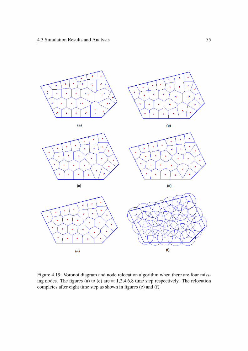
4.3 Simulation Results and Analysis 55
Figure 4.19: Voronoi diagram and node relocation algorithm when there are four miss-ing nodes. The figures (a) to (e) are at 1,2,4,6,8 time step respectively. The relocationcompletes after eight time step as shown in figures (e) and (f).

Chapter 5
Conclusion and Future Work
This thesis has presented different algorithms for area coverage problem. The algo-rithms are divided into non-communicative and communicative area coverage. In non-communicative, the UAV agents perform the assigned tasks disjointedly by sweepingover the region of interest. They follow the partitioned regions and routes assigned bythe base station. In communicative area coverage, the agents spread over the region ofinterest. They sense regions within their sensing range and are able communicate to thenodes within their communication range. This area coverage can monitor the region atlonger time and send the data to the base station in near real time. However, it requiresmore agents to perform the task.
In non-communicative area coverage, a polygon area decomposition algorithm is pro-posed. The algorithm intends for a setting where the UAV agents have to start and endthe area coverage at the same base station. The region of interest is a simple, non-convexpolygon. The algorithm considers geometry of the polygon before decomposing the re-gion. It starts the decomposition at the longest side of the polygon with partitioning linesegment parallel to the longest side. The algorithm assigns the partitioning line segmentto be parallel to the longest side of the polygon for the smaller minimum diameter func-tion. The results show that a partitioned region always gives less or equal number ofturns compared to a partitioned region from [15]. Moreover, the algorithm also givesless overlapped areas since all the partitioned regions have one side connected to thebase station.
The proposed algorithm is for a situation where a region of interest is a convex polygonwithout any holes or obstacles. However, there could be a situation where the agentshave to avoid obstacles in some area inside the region of interest. There exist algorithmsfor partitioning the polygons with obstacles, but none of them considers a situationwhere the agents have to start and end the routes at the same base station. Figure 5.1illustrates examples of a polygon with an obstacle. The figures show possible ways to
56

Chapter 5: Conclusion and Future Work 57
Figure 5.1: Examples of partition of a polygon with obstacle.
partition the polygon.
The potential future work of this area decomposition with or without obstacles could besimulating the sweeping area coverage in virtual situation using simulating tools suchas USARSim. The simulation would give quantitative comparison between the twoalgorithms and yield parameters such as appropriate flying height or maximum flyingdistance.
In non-communicative area coverage, the overall task cannot be completed if one agentfails to perform its mission. The agent might be broken down or lost without any aware-ness from its team member or the base station. On the contrary, all the agents and thebase station are connected in communicative area coverage. The base station knows the

Chapter 5: Conclusion and Future Work 58
agents’ status and locations for more robust and real time area coverage.
The algorithms presented in communicative area coverage are static and dynamic posi-tioning. Static positioning predetermined the node positions according to sensing rangeof the node and region of interest. The positioning gives fast but non-adaptable nodedeployment. In finding minimum number of nodes that fully cover the region of inter-est, hexagonal tiling is used to provide approximate number and positions of the nodes.The distance between a node at the center of a hexagon and its adjacent neighbors areequal in all directions.
Dynamic positioning assists the area coverage when the nodes are randomly distributedor when there is a potential node failure. In this work, three algorithms were studiedand applied to predetermined node locations where there is one or more nodes missing.The algorithms are DSSA, VDDA, and the centroid-based scheme. DSSA relocationis not suitable for the mentioned setting since boundary of the region of interest is notconsidered in the algorithm. The nodes near the boundary tend to move out of the regionaccording to partial forces exerted from their neighbors.
VDDA and centroid-based scheme algorithms use Voronoi diagram to determine theregion the node has to cover. Hence, the algorithms can limit the node movement towithin a region of interest by considering only the Voronoi diagram that intersects withthe region of interest. VDDA algorithm searches for the location that gives maximalutility gain which is the product of effective area covered by the node at its new locationand the estimated lifetime when the node moves to the new location. When applyingVDDA to the predetermined node locations with one or more missing nodes, most of thenodes remain at their current locations. This is because the locations are predeterminedand the current locations already give maximal utility gain.
The centroid-based scheme is applicable to this setting. When there is a missing node,the Voronoi region of its neighboring node is bigger than its sensing region. The neigh-boring node moves to the centroid of its Voronoi region. The direction of the centroid istoward missing the node’s direction. Hence, the nodes compensate the missing one andfully cover the region of interest after some rounds of relocation. The time spending onnode relocation depends on the number of missing nodes and position of the missingnodes. The location of the missing node that has more adjacent neighbors requires lesstime to relocate than the location that has fewer adjacent neighbors. This relocation al-gorithm functions properly as long as the number of working nodes is not less than theminimum number of nodes required to completely cover the region of interest.

Chapter 5: Conclusion and Future Work 59
The communicative area coverage in this thesis considers only the positioning algo-rithm. Nevertheless, the aspects related to communication should also be concerned inthe actual situation. For example, the number of hops in multi-hop wireless ad hoc net-work, the communication delay, ad hoc routing algorithm, and etc. These factors affectthe efficiency of the area coverage and should be studied further.


List of Figures
2.1 Steps for polygon area decomposition . . . . . . . . . . . . . . . . . . 102.2 Sensing capability [22] . . . . . . . . . . . . . . . . . . . . . . . . . . 122.3 The number of turns along different sweep directions [17] . . . . . . . . 132.4 An example of diameter function [19] . . . . . . . . . . . . . . . . . . 142.5 Diameter of a polygon at different angles [19] . . . . . . . . . . . . . . 15
3.1 Polygon area decomposition using geometry-based algorithm . . . . . . 183.2 Regions of interest with different side of the longest side L . . . . . . . 203.3 Partitioned regions of different polygons . . . . . . . . . . . . . . . . . 213.4 Diameter functions of subregions partitioned using different algorithm . 223.5 Diameter functions of subregions partitioned using different algorithm . 233.6 Examples of partitioned regions . . . . . . . . . . . . . . . . . . . . . 233.7 Route comparison of the same polygon but with different start position . 253.8 Different width of partitioned regions . . . . . . . . . . . . . . . . . . 263.9 Route comparison of the same polygon but with different algorithm . . 273.10 Area decomposition and route generation of a polygon using different
algorithms . . . . . . . . . . . . . . . . . . . . . . . . . . . . . . . . . 28
4.1 Different clustering shapes . . . . . . . . . . . . . . . . . . . . . . . . 314.2 Regular hexagonal tiling and the nodes sensing regions . . . . . . . . . 324.3 Node locations and their sensing regions . . . . . . . . . . . . . . . . . 334.4 First layer of hexagonal tiling . . . . . . . . . . . . . . . . . . . . . . . 334.5 Dimension of hexagons . . . . . . . . . . . . . . . . . . . . . . . . . . 344.6 Adjusted hexagonal tiling and their sensing regions . . . . . . . . . . . 354.7 Node placement . . . . . . . . . . . . . . . . . . . . . . . . . . . . . . 354.8 Hexagonal tiling when considers different first layer . . . . . . . . . . . 364.9 Example of DSSA node movement [14] . . . . . . . . . . . . . . . . . 414.10 Example of DSSA node movement with a failed node [14] . . . . . . . 424.11 Voronoi diagram . . . . . . . . . . . . . . . . . . . . . . . . . . . . . 434.12 Node placement with sensing range 80% of its maximum sensing range 494.13 Node repositioning using DSSA algorithm . . . . . . . . . . . . . . . . 50
61

List of Figures 62
4.14 Voronoi diagram of nodes at predetermined locations . . . . . . . . . . 514.15 Voronoi diagram of predetermined locations with one missing node . . 514.16 Nodes relocation at four time steps . . . . . . . . . . . . . . . . . . . . 534.17 Nodes locations and their sensing regions after the algorithm . . . . . . 544.18 Predetermined node locations with four missing nodes . . . . . . . . . 544.19 Node relocation algorithm of four missing nodes . . . . . . . . . . . . 55
5.1 Area partition of polygons with obstacles . . . . . . . . . . . . . . . . 57


Bibliography
[1] A. Agarwal, L. M. Hiot, E. M. Joo, and N. T. Nghia. Rectilinear workspace parti-tioning for parallel coverage using multiple uavs.
[2] T. Asano and T. Asano. Minimum partition of polygonal regions into trapezoids. InProceedings of the 24th Annual Symposium on Foundations of Computer Science,SFCS ’83, pages 233–241, 1983.
[3] F. Aurenhammer. Voronoi diagrams a survey of a fundamental geometric datastructure. ACM Comput. Surv., 23(3):345–405, Sept. 1991.
[4] Y. Bouktir, M. Haddad, and T. Chettibi. Trajectory planning for a quadrotor heli-copter. 2008 16th Mediterranean Conference on Control and Automation, pages1258–1263, 2008.
[5] B. M. Chazelle. Computational geometry and convexity. PhD thesis, New Haven,CT, USA, 1980. AAI8110021.
[6] C. Chen and R.-C. Chang. On the minimality of polygon triangulation. BIT,30(4):570–582, 1990.
[7] A. Clot and R. S. L. M. G. Britain). Communications Command and Control.Defense Technical Information Center, 2000.
[8] L. de Floriani and E. Puppo. An On-Line Algorithm for Constrained DelaunayTriangulation. GMIP, 54(4):290–300, July 1992.
[9] P. A. Devijver and S. Maybank. On the computation of the delaunay triangulationof a convex polygon. In Proc. 6th IEEE Internat. Conf. Pattern Recogn., pages420–422, 1982.
[10] S. Fowers. Stabilization and control of a quad-rotor micro-uav using vision sen-sors. PhD thesis, 2008.
[11] D. H. Greene. The decomposition of polygons into convex parts. ComputationalGeometry, Advances in Computing Research, 1:235–259, 1983.
64

Bibliography 65
[12] M. Günes and O. Spaniol. Routing Algorithms for Mobile Multi-Hop Ad-HocNetworks. In H. Turlakov and L. Boyanov, editors, Proceedings of Next Genera-tion Network Technologies International Workshop, pages 10–24 October, October2002.
[13] N. Heo and P. Varshney. A distributed self spreading algorithm for mobile wire-less sensor networks. In Wireless Communications and Networking, 2003. WCNC2003. 2003 IEEE, volume 3, pages 1597 –1602 vol.3, 2003.
[14] N. Heo and P. Varshney. Energy-efficient deployment of intelligent mobile sensornetworks. Systems, Man and Cybernetics, Part A: Systems and Humans, IEEETransactions on, 35(1):78 – 92, 2005.
[15] S. Hert and V. Lumelsky. Polygon area decomposition for multiple-robotworkspace division. International Journal of Computational Geometry and Ap-plications, 8:437–466, 1998.
[16] G. M. Hoffmann, S. L. Waslander, and C. J. Tomlin. Electrical Engineering,44(August):1–14, 2008.
[17] W. H. Huang. Optimal line-sweep-based decompositions for coverage algorithms.In Proceedings IEEE International Conference on Robotics & Automation, pages27–32, 2001.
[18] J. M. Keil. Decomposing a polygon into simpler components. SIAM Journal onComputing, 14:799–817, 1985.
[19] P. D. R. Klein. Geometry lab: The diameter function of an arbitrary polygon.http://web.cs.uni-bonn.de/I/GeomLab/Diameter/index.html.en. [On-line; accessed 28-Dec-2011].
[20] H.-J. Lee, Y. hwan Kim, Y.-H. Han, and C. Y. Park. Centroid-based movementassisted sensor deployment schemes in wireless sensor networks. In VTC Fall,pages 0–, 2009.
[21] C. Levcopoulos and A. Lingas. Bounds on the length of convex partitions ofpolygons. In Proceedings of the Fourth Conference on Foundations of SoftwareTechnology and Theoretical Computer Science, pages 279–295, London, UK, UK,1984. Springer-Verlag.
[22] I. Maza and A. Ollero. Multiple uav cooperative searching operation using poly-gon area decomposition and efficient coverage algorithms. In Proceedings of the7th International Symposium on Distributed Autonomous Robotic Systems, pages211–220, 2004.

Bibliography 66
[23] A. Mukherjee, S. Bandyopadhyay, and D. Saha. Radio propagation. In Loca-tion management and routing in mobile wireless networks, Artech House mobilecommunications series, pages 32–37. Artech House, 2003.
[24] I. Redbooks. Wireless lan performance. In Local Area Network Concepts andProducts: Adapters, Hubs and Atm. Vervante, 1996.
[25] S. B. Tor and A. E. Middleditch. Convex decomposition of simple polygons. ACMTrans. Graph., 3(4):244–265, 1984.
[26] H. ur Rehman. Multihop connectivity in wireless ad hoc networks. PhD thesis.
[27] D. Wang, L. Xu, J. Peng, and S. Robila. Subdividing hexagon-clustered wirelesssensor networks for power-efficiency. In Proceedings of the 2009 WRI Interna-tional Conference on Communications and Mobile Computing - Volume 02, CMC’09, pages 454–458, Washington, DC, USA, 2009. IEEE Computer Society.
[28] M. Younis and K. Akkaya. Strategies and techniques for node placement in wire-less sensor networks: A survey. Ad Hoc Netw., 6(4):621–655, June 2008.