approximation algorithms for sweep coverage in wireless
TRANSCRIPT

Approximation Algorithms for SweepCoverage in Wireless Sensor Networks
Thesis submitted in partial fulfillment of
the requirements for the degree of
Doctor of Philosophy
by
Barun Gorain
(Roll No. 10612305)
Under the Supervision of
Dr. Partha Sarathi Mandal
to the
Department of Mathematics
Indian Institute of Technology Guwahati
Guwahati - 781039, India
August 2015

TH-1437_10612305

CERTIFICATE
This is to certify that this thesis entitled “Approximation Algorithms for Sweep
Coverage in Wireless Sensor Networks” being submitted by Mr. Barun Gorain to
the Department of Mathematics, Indian Institute of Technology Guwahati, is a record
of bona fide research work under my supervision and is worthy of consideration for the
award of the degree of Doctor of Philosophy of the Institute.
The results contained in this thesis have not been submitted in part or full to any
other university or institute for the award of any degree or diploma.
Place: IIT Guwahati Dr. Partha Sarathi Mandal
Date: Department of Mathematics
Indian Institute of Technology Guwahati
Guwahati-781039, Assam, India
iii
TH-1437_10612305

TH-1437_10612305

ACKNOWLEDGEMENTS
The completion of this study required the help and goodwill of various individuals.
Without them, I might not have met my objective of doing this study. I would like to
express my gratitude to the following people for their invaluable help and support.
It would be very unfair if I did not begin this note of acknowledgement without
mentioning my supervisor Dr. Partha Sarathi Mandal. I am very grateful to him for
his invaluable guidance, utmost care and constant encouragement throughout this work.
All of my queries have been listened with patience and answered with profound clarity.
I would like to thank him for carefully reading my thesis, providing useful feedbacks
and posing interesting questions. I am also thankful to him for making me feel free to
express my views and for sharing an excellent relationship with me. I could not have
imagined having a better supervisor and mentor for my doctoral study. He and Boudi,
Dr. Debarati Mitra, along with Kaushik da always treated me like family members. We
enjoyed a lot together in the occasional lunch and dinner parties.
I owe my thanks to the doctoral committee members Prof. Sukumar Nandi, Prof.
Diganta Goswami and Dr. Kalpesh Kapoor for their valuable comments and suggestions
on my work. I would also like to thank Indian Institute of Technology Guwahati for the
facilities provided to me during my research work and to the Ministry of Human and
Resource Development, Govt. of India, for the financial assistance. I offer my sincere
thanks to our lab assistant Mr. Santanu Majumdar and Mr. Pranpratim Borgohain for
technical supports. Sridhar Samal and Phatik Kumar of the Department of Mathematics
deserve special thanks for their assistance in all of the official matters.
I owe my thanks to Prof. Sandip Das from ISI Kolktata for his valuable suggestions
and comments on my works. I would like to thank Dr. Stefan Schmid and Prof. Krish-
nendu Mukhopadhaya for their valuable comments and suggestions. I would also like to
thank Dr. Gautam Das and Dr. Anjan K. Chakrabarty for inspiring me throughout my
stay in IITG. I owe my sincere thanks to Dr. Debarati Mitra for her constant support
and care all along these years.
I wish to thank all my friends and well-wishers for their love and encouragement dur-
ing this period. I would like to thank Kaushik Da, Arnab Da, Kalyan, Santu Da, Gowri
Da, Punit, Abhishek, Anirban, Debopam, Kalyan Da, Punu da, Niladri da, Mandar da,
v
TH-1437_10612305

sibu da and Hiranmoy for making my stay at IITG enjoyable and comfortable. Instead
of being so far from my family, their company never made me feel alone in the campus.
The memories of playing cricket in the weekends and having the delicious chicken parties
are irreplaceable.
Himadri da deserves a special thanks for his immense help from my MSc days to the
last day of my PhD. Whenever I was facing any problem, Hiamadri da was always there
to solve those problems immediately. I thank Deva and Murali da for their constant
support throughout all these years. Despite being not present in Guwahati, they always
spared time to talk and encourage me.
I would like to express my respect to all my relatives and neighbours for their best
wishes. I am very much thankful to Boro Kaku, Boro Kakima for their love and care from
my childhood days. I feel myself lucky to have a wonderful family with lovely brothers
and sisters. I thank Amit da, Tublu, Mousumi and Romu da for always motivating me
to do better. I specially thank Somu da for believing in me and motivating me to do my
best. Without his guidance and support, I may not be in the position today I am. My
elder brother and my sisters deserve special thanks for their love and care throughout
my life.
Last but not the least, I would like to extend my deepest gratitude to my parents
without whose love, support and understanding I could never have completed this doc-
toral degree. Their support has been unconditional all these years. They have cherished
with me every great moment and supported me whenever I needed it.
Finally, I finish by thanking all my well wishers whose names are not listed here.
Place: IIT Guwahati
Date: Barun Gorain
vi
TH-1437_10612305
ABSTRACT
Coverage is one of the most important issues in wireless sensor networks (WSNs) and it
is a well studied research area. To ensure coverage, a set of sensors continuously monitor
the subject to be covered. Sweep coverage is a recent development for the applications
of WSNs where periodic monitoring by a set of mobile sensors is sufficient instead of
continuous one like traditional coverage. In this thesis, we remark on the flaw of the
approximation algorithms [41] for sweep coverage for a set of points. We propose a
3-approximation algorithm to guarantee sweep coverage for the vertices of a weighted
graph, where vertices are considered as the set of points. When vertices of the graph
have different sweep periods and processing times, we propose a O(log ρ)-approximation
algorithm as a solution, where ρ is the ratio of the maximum and minimum sweep
periods among the vertices. If speeds of the mobile sensors are different, we prove
that it is impossible to design any constant factor approximation algorithm to solve the
problem, unless P=NP.
Energy is an important issue for the sensors. To incorporate it, an energy efficient
sweep coverage problem is proposed, where a combination of static and mobile sensors
are used. The problem is NP-hard and cannot be approximated within a factor of 2,
unless P=NP. An 8-approximation algorithm is proposed to solve it. A 2-approximation
algorithm is also proposed for a special case of the problem, which is the best possible
approximation factor. Energy utilization for the mobile sensors is restricted as they
are battery-powered. Considering the limitation, an energy restricted sweep coverage
problem is defined and a (5 + 2α)-approximation algorithm is proposed to solve this
NP-hard problem. Periodic patrol inspection is important to detect illegal movement
across national border. A portion of border can be modeled as a finite length curve.
With this model, we introduce barrier sweep coverage concept for periodic monitoring
of finite length curves in two dimensional plane. A solution is proposed to sweep cover a
finite length curve with optimal number of mobile sensors. An energy restricted barrier
sweep coverage problem is introduced and proposed a 133-approximation algorithm for a
finite length curve. We prove that finding minimum number of mobile sensors to sweep
coverage for a set of finite length curves is NP-hard and cannot be approximated within
a factor of 2. For that a 5-approximation algorithm is proposed. A 2-approximation
vii
TH-1437_10612305

algorithm is also proposed to solve the problem for a special case, where each mobile
sensor must visit all points of each curve. We formulate a data gathering problem by a
set of data mules and prove that the problem is NP-hard. A 3-approximation algorithm
is proposed to solve it. Through simulation, performance of the algorithm for multiple
finite length curves is investigated. We introduce area sweep coverage problem and prove
that the problem is NP-hard. A 2√2-approximation algorithm is proposed to solve
the problem for a square region. For arbitrary bounder region A the approximation
factor is 2(√
2 + 2rPArea(A)
)
, where P is the perimeter of A and r is sensing range of
the mobile sensors. Through simulation, we analyze performance of the algorithm for
area bounded by arbitrary simple polygons. We propose a distributed sweep coverage
problem, where static sensors are placed at the location of PoIs, one for each. In our
proposed algorithm, the static sensors themselves decide number with initial positions as
well as movement strategy of the mobile sensors through message passing. The mobile
sensors visit the static sensors once in a given time period to sweep cover the PoIs. The
proposed algorithm achieved an approximation factor of 4. A 2-approximation algorithm
is also proposed for a special case of the problem.
viii
TH-1437_10612305

Contents
1 Introduction 1
1.1 Scope of the Thesis . . . . . . . . . . . . . . . . . . . . . . . . . . . . . . 4
1.1.1 Sweep coverage for a set of points . . . . . . . . . . . . . . . . . . 4
1.1.2 Sweep coverage with heterogeneity . . . . . . . . . . . . . . . . . 5
1.1.3 Solving energy issues for sweep coverage . . . . . . . . . . . . . . 5
1.1.4 Area sweep coverage . . . . . . . . . . . . . . . . . . . . . . . . . 5
1.1.5 Barrier sweep coverage . . . . . . . . . . . . . . . . . . . . . . . . 6
1.1.6 Distributed sweep coverage . . . . . . . . . . . . . . . . . . . . . . 6
2 Review of Related Works 7
2.1 Introduction . . . . . . . . . . . . . . . . . . . . . . . . . . . . . . . . . . 7
2.2 Static coverage . . . . . . . . . . . . . . . . . . . . . . . . . . . . . . . . 7
2.2.1 Point coverage . . . . . . . . . . . . . . . . . . . . . . . . . . . . . 7
2.2.2 Area coverage . . . . . . . . . . . . . . . . . . . . . . . . . . . . . 9
2.2.3 Barrier coverage . . . . . . . . . . . . . . . . . . . . . . . . . . . . 11
2.3 Sweep coverage . . . . . . . . . . . . . . . . . . . . . . . . . . . . . . . . 12
3 Sweep Coverage for a Set of Points 15
3.1 Introduction . . . . . . . . . . . . . . . . . . . . . . . . . . . . . . . . . . 15
3.1.1 Contribution . . . . . . . . . . . . . . . . . . . . . . . . . . . . . 16
3.2 2-Approximation Algorithm for a Special Case . . . . . . . . . . . . . . . 16
3.3 Sweep Coverage on a Weighted Graph . . . . . . . . . . . . . . . . . . . 18
3.3.1 Analysis . . . . . . . . . . . . . . . . . . . . . . . . . . . . . . . . 19
3.4 Sweep Coverage in Presence of Obstacles . . . . . . . . . . . . . . . . . . 22
ix
TH-1437_10612305

3.5 Simulation . . . . . . . . . . . . . . . . . . . . . . . . . . . . . . . . . . . 23
3.6 Conclusion . . . . . . . . . . . . . . . . . . . . . . . . . . . . . . . . . . . 27
4 Sweep Coverage with Heterogeneity 29
4.1 Introduction . . . . . . . . . . . . . . . . . . . . . . . . . . . . . . . . . . 29
4.1.1 Contribution . . . . . . . . . . . . . . . . . . . . . . . . . . . . . 29
4.2 Sweep Coverage with Different Sweep Periods and Processing Times . . . 30
4.2.1 Proposed algorithm . . . . . . . . . . . . . . . . . . . . . . . . . . 31
4.2.2 Analysis . . . . . . . . . . . . . . . . . . . . . . . . . . . . . . . . 33
4.3 Inapproximability of Sweep Coverage with Mobile Sensors having Differ-
ent Speeds . . . . . . . . . . . . . . . . . . . . . . . . . . . . . . . . . . . 34
4.4 Conclusion . . . . . . . . . . . . . . . . . . . . . . . . . . . . . . . . . . . 36
5 Solving Energy Issues for Sweep Coverage 37
5.1 Introduction . . . . . . . . . . . . . . . . . . . . . . . . . . . . . . . . . . 37
5.1.1 Contribution . . . . . . . . . . . . . . . . . . . . . . . . . . . . . 38
5.2 Energy Efficient Sweep Coverage Problem . . . . . . . . . . . . . . . . . 38
5.2.1 Algorithm and Analysis . . . . . . . . . . . . . . . . . . . . . . . 40
5.2.2 A special case of ESweep coverage problem . . . . . . . . . . . . . 44
5.3 Energy Restricted Sweep Coverage Problem . . . . . . . . . . . . . . . . 45
5.3.1 Algorithm and Analysis . . . . . . . . . . . . . . . . . . . . . . . 47
5.4 Conclusion . . . . . . . . . . . . . . . . . . . . . . . . . . . . . . . . . . . 51
6 Area Sweep Coverage 53
6.1 Introduction . . . . . . . . . . . . . . . . . . . . . . . . . . . . . . . . . . 53
6.1.1 Contribution . . . . . . . . . . . . . . . . . . . . . . . . . . . . . 53
6.2 Area Sweep Coverage Problem . . . . . . . . . . . . . . . . . . . . . . . . 54
6.3 Solution of Area Sweep Coverage . . . . . . . . . . . . . . . . . . . . . . 54
6.3.1 Analysis . . . . . . . . . . . . . . . . . . . . . . . . . . . . . . . . 55
6.4 Improved Solution for Rectangular Region . . . . . . . . . . . . . . . . . 57
6.5 Solution for Arbitrary Bounded Region . . . . . . . . . . . . . . . . . . . 58
6.6 Simulation . . . . . . . . . . . . . . . . . . . . . . . . . . . . . . . . . . . 59
x
TH-1437_10612305

6.7 Conclusion . . . . . . . . . . . . . . . . . . . . . . . . . . . . . . . . . . . 61
7 Barrier Sweep Coverage 63
7.1 Introduction . . . . . . . . . . . . . . . . . . . . . . . . . . . . . . . . . . 63
7.1.1 Contribution . . . . . . . . . . . . . . . . . . . . . . . . . . . . . 63
7.2 Problem Definitions . . . . . . . . . . . . . . . . . . . . . . . . . . . . . . 64
7.3 Barrier Sweep Coverage for a finite Curve . . . . . . . . . . . . . . . . . 65
7.3.1 Optimal solution for a finite curve . . . . . . . . . . . . . . . . . . 65
7.3.2 Energy restricted barrier sweep coverage . . . . . . . . . . . . . . 66
7.4 Barrier Sweep Coverage for Multiple finite Curves . . . . . . . . . . . . . 72
7.4.1 2-approximation solution for a special case . . . . . . . . . . . . . 72
7.4.2 Solution for BSCMC . . . . . . . . . . . . . . . . . . . . . . . . . 75
7.5 Data Gathering by Data Mules . . . . . . . . . . . . . . . . . . . . . . . 77
7.5.1 Analysis . . . . . . . . . . . . . . . . . . . . . . . . . . . . . . . . 80
7.6 Simulation Results . . . . . . . . . . . . . . . . . . . . . . . . . . . . . . 81
7.7 Conclusion . . . . . . . . . . . . . . . . . . . . . . . . . . . . . . . . . . . 83
8 Distributed Sweep Coverage 85
8.1 Introduction . . . . . . . . . . . . . . . . . . . . . . . . . . . . . . . . . . 85
8.1.1 Contribution . . . . . . . . . . . . . . . . . . . . . . . . . . . . . 86
8.2 Approximation for a Special Case of Distributed Sweep Coverage . . . . 86
8.2.1 System Model and Algorithm . . . . . . . . . . . . . . . . . . . . 86
8.3 4-approximation Algorithm for Distributed Sweep Coverage . . . . . . . . 88
8.4 Conclusion . . . . . . . . . . . . . . . . . . . . . . . . . . . . . . . . . . . 90
9 Conclusion 91
xi
TH-1437_10612305

TH-1437_10612305

Chapter 1
Introduction
In last few decades, immense achievements in wireless sensor networks (WSNs) took
place due to their wide range of potential applications. WSNs are used in almost every
aspects of real life applications such as general engineering, agriculture & environmental
monitoring, civil engineering, military applications, health monitoring & surgery, etc. A
sensor node or in short, sensor is a battery-powered small autonomous device consisting
of a sensing unit, small processor, memory and transceiver. It is capable of sensing
physical or environmental conditions within its sensing range. A sensor can communicate
with other sensors through radio frequency channels within its communication range.
Once sensors are deployed over a region of interest, they form a wireless network with
their self-organization capacities. Sensors monitor physical or environmental conditions
like light, temperature, humidity, motion of objects, etc., and cooperatively send data
through the network to a sink. The sink provides a user interface to interact with
the user. The WSN provides an opportunity to monitor objects remotely. There are
several issues of designing hardware of a sensor such as power source, memory capacity,
processor speed, range of communication, size of a sensor node, manufacturing cost,
etc. In spite of having sensors with the given specifications, there are several challenges
on theoretical modeling, design of energy-efficient protocols, capacity/throughput of a
network, localization, routing, coverage, channel access and scheduling, connectivity,
quality of service, security, implementation, etc. Out of them, coverage is one of the
most important challenge of the WSNs. The fundamental question of the coverage
1
TH-1437_10612305

problem is “how well do the sensors observe physical space?”. The main objective of
coverage problem is to cover the subjects by the sensing range of the sensors. For
example, in forest monitoring [1], every location of the forest must be covered by at
least one sensor in order to detect any unusual activities like forest fire, activities of
poachers, etc. immediately. Similarly, covering boundary of the forest allows controlling
and elimination of the poaching activities, and illegal entry through the boundary. A
similar notion of coverage is termed as k-coverage [33, 36, 40], where instead of one
sensor, the subjects of interest must be within the sensing range of at least k sensors.
There are different aspects that are needed to be considered for designing suitable
coverage algorithms for different applications. Mainly, there are three types of coverage
problem found in literature. The first one is point coverage or target coverage [7, 9, 11,
67, 69], where a set of points, called targets are to be covered by a set of sensors. The
second one is the area coverage [3, 44, 52, 57, 62, 63], where each and every point inside
a bounded region is to be covered by a set of sensors. The other type of problem is called
barrier coverage [33, 35, 36, 40, 42, 49, 50, 51, 54], where the objective is to secured the
boundary of a region by covering a set of sensors.
Coverage problems are studied in the area of computational geometry for many years
before the devolvement of WSNs. Some of the most popular problems are the art gallery
problem, packing and covering of geometric objects, etc. The objective of art gallery
problem [21, 26] is to determine the number of guards and their locations to cover an
art gallery such that every point of the gallery is visible by at least one guard. There
are several variations of this problem depending on the restrictions of placement of the
guards provided the art gallery is of a polygonal structure. These variations are named as
vertex guard, edge guard and point guard. In vertex guard, the guards are to be placed
on the vertices of the polygonal gallery. In edge guard, the guards are to be placed on
the edges of the polygonal gallery and in the point guard, the guards are to be placed
on any point inside the polygonal gallery. All these variations of the problem are known
to be NP-hard. The packing and covering problems [27] are studied in computational
geometry for last six or seven decades. Objective of the packing problems is to pack
a given area with minimum number of objects of a given shape like circle, square or
hexagon without overlapping. In the covering problem, the objects can be overlapped
2
TH-1437_10612305

and the objective is to cover the given area with minimum number of objects.
For the aforementioned problems, where coverage are maintained continuously, termed
as static coverage [41]. But there are typical applications where only periodic patrol in-
spections are sufficient for a certain set of points of interest instead of continuous mon-
itoring like static coverage. This type of coverage is termed as sweep coverage. First,
theoretical aspects of the sweep coverage problem is studied by Li et al. [41], where peri-
odic patrol inspections are required for a given set of points of interest (PoIs) by a set of
mobile sensors. Unlike static coverage, in sweep coverage, the coverage requirement for
the PoIs are time variant. Therefore, the solutions of static coverage problems cannot
be applied for sweep coverage as they may lead to an unnecessary extra overhead and
poor efficiency.
As per the model [41] for sweep coverage, the mobile sensors are assumed point
sensors. So, the mobile sensor should reach at the position of a point of interest (PoI) to
cover it at a time instance. A point is said to be t-sweep covered if and only if at least one
mobile sensor visits the point within every t time period, where t is called sweep period
of the point. The objective of the sweep coverage problem is to find minimum number
of mobile sensors to guarantee sweep coverage for a given set of PoIs. Sweep coverage is
useful for many real life applications like periodic health checkup, periodic automobile
servicing, periodic inspection of boilers/pressure vessels in industry, periodic monitoring
to secure target locations, periodic data gathering for agriculture and environmental
monitoring, etc. Let us consider a practical scenario for data gathering, where a set
of static sensors are deployed over a region of interest to collect information from the
region. If the size of the data is high, it is expensive to send the data through message
passing to the sink and it is more useful to collect data from the individual sensors. A
mobile sensor can collect the data stored at a static sensor and deliver it to the sink.
Also, having limited storage capacity of the static sensors, a mobile sensor must visit the
static sensors frequently and collect data to avoid significant data loss. In this scenario,
sweep coverage is useful. In this case, a static sensor is visited by a mobile sensor at
least once in every predefined time period and the mobile sensors collect data from the
static sensors.
As we have already mentioned, there are three types of static coverage problems
3
TH-1437_10612305
depending on the subject to be covered by the sensors. Designing suitable sweep coverage
algorithms for those variations are challenging problems. On sweep coverage, there are
many works exist in literature for a set of discrete points. Most of the existing works [14,
19, 41, 55, 61, 64, 66, 68] focus on designing heuristics. Li et al. [41] formally defined the
problem for a set of points and analyzed it from a theoretical point of view. They proved
that the sweep coverage problem is NP-hard and cannot be approximated within a factor
of 2, unless P=NP. The authors proposed constant factor approximation algorithms to
solve the problem. But there is a serious flaw in the approximation algorithm [41]. This
motivates us to design a constant factor approximation algorithm for sweep coverage
problem by correcting the flaw of the previous work. Further, it will be interesting to
investigate the sweep coverage problem in the context of barrier coverage, area coverage
problems. It also might be interesting to design sweep coverage for distributed setting.
There are several challenges for designing sweep coverage algorithms. These are fault
tolerance [6], energy efficiency [9], self-stabilization [5, 47], scalability [43], etc.
1.1 Scope of the Thesis
In this thesis, we introduce and analyze several sweep coverage problems depending
on various theoretical and practical aspects. Most of the sweep coverage problems we
consider are NP-hard. So, our focus is to design suitable approximation algorithms for
those problems.
1.1.1 Sweep coverage for a set of points
In Chapter 3, we remark on the flaw of the approximation algorithm proposed in the
paper [41] for a set of PoIs and propose a 3-approximation algorithm to guarantee sweep
coverage. As the previous approximation algorithm is not correct, to the best of our
knowledge, we are the first to design constant factor approximation algorithm for the
sweep coverage problem. A 2-approximation algorithm is proposed for a special case of
the problem, where every PoI must be visited by each of the mobile sensors. A solution
for sweep coverage in presence of obstacles is also proposed.
4
TH-1437_10612305

1.1.2 Sweep coverage with heterogeneity
In Chapter 4, we propose an algorithm to solve the sweep coverage problem when dif-
ferent PoIs are having different sweep periods and processing times. Our proposed
algorithm achieves approximation factor O(log ρ), where ρ is the ratio of maximum and
minimum sweep periods. We also investigate the problem when speed of the mobile
sensors are different. We prove that it is impossible to design any constant factor ap-
proximation algorithm for sweep coverage problem with mobile sensors having different
speeds, unless P=NP.
1.1.3 Solving energy issues for sweep coverage
In Chapter 5, we introduce an energy efficient sweep coverage problem where a combi-
nation of static and mobile sensors are used to sweep cover a given set of PoIs. An 8-
approximation algorithm is proposed to solve this NP-hard problem. A 2-approximation
algorithm is proposed for a special case of the problem where all mobile sensors visit
the same subset of PoIs, while for the remaining PoIs, static sensors are used. Then we
introduce another variation of sweep coverage, called energy restricted sweep coverage
problem and propose a (5+ 2α)-approximation algorithm to solve this NP-hard problem.
1.1.4 Area sweep coverage
The sweep coverage problem for a bounded area is introduced in Chapter 6. We prove
that the area sweep coverage problem is NP-hard. A 2√2-approximation algorithm is
proposed for a square region. The approximation factor is further improved for rectan-
gular region. For arbitrary bounded region, the approximation factor of our proposed
algorithm is a function of area, perimeter of the region and the sensing range of the mo-
bile sensors. Through simulation, we analyze performance of the algorithm for randomly
generated simple polygons.
5
TH-1437_10612305

1.1.5 Barrier sweep coverage
In Chapter 7, we introduce barrier sweep coverage problem, where a barrier is rep-
resented by a finite length continuous curve. We propose optimal solution for sweep
coverage of a single curve. We introduce an energy restricted sweep coverage problem
for single curve and propose a 133-approximation algorithm. For multiple curves in a
plane, we propose a 5-approximation algorithm for barrier sweep coverage problem and
a 2-approximation algorithm for a special case of the problem. As an application of
barrier sweep coverage problem, we formulate a data gathering problem and propose a
3-approximation algorithm to solve it.
1.1.6 Distributed sweep coverage
Li et al. [41] commented on the impossibility of designing distributed sweep coverage
algorithm for a given set of PoIs. In Chapter 8, we propose a distributed sweep coverage
in a different context. We assume static sensors are placed at the location of the PoIs,
one for each. The set of static sensors forms a network. The static sensors decide the
initial positions and movement strategy of the mobile sensors through message passing.
A set of mobile sensors visits the static sensors once in a given time period to sweep cover
the static sensors. We introduce a distributed sweep coverage problem and propose a
4-approximation algorithm. A 2-approximation algorithm is also proposed for a special
case of the problem.
6
TH-1437_10612305

Chapter 2
Review of Related Works
2.1 Introduction
Coverage is a well-studied area of research in WSNs. But time-variant coverage in WSN
is developed recently. Based on the dimension of time, coverage can be classified into
two categories such as static coverage and sweep coverage. In static coverage, generally
subjects are monitored by a set of sensors all along without any interruption whereas
in sweep coverage subjects are monitored by a set of mobile sensors periodically. In
this chapter, we briefly describe recent contributions that addressed different coverage
problems in the context of our contributions in this thesis.
2.2 Static coverage
In static coverage, sensors continuously monitor subjects after deployment. Depending
on the types of the subjects to be covered, the static coverage is classified into three
categories in literature. Those are point coverage, area coverage, and barrier coverage.
Each category is reviewed separately in the following sections.
2.2.1 Point coverage
Most of the works found in literature on point or target coverage problems are focused
on maximizing network lifetime. Since the sensors are equipped with limited battery,
7
TH-1437_10612305

recharging or replacing the battery may not always viable for applications in remote
areas. In order to extend lifetime of the network and hence lifetime of the sensors, the
set of sensors are divided into several disjoint subsets. The subsets are made in such a
way that each PoI is in the sensing range of several sensors belonging to several subsets.
The network lifetime can be extended with proper sleep-wake-up scheduling among the
subsets of the sensors.
In paper [9], authors model the discrete target coverage problem as a disjoint set
cover problem and proved that the problem is NP-complete. The disjoint set cover
problem is transformed into a maximum flow problem. A heuristic is proposed using
mixed integer programming to solve the maximum flow problem. Cardei et al. [8]
improved the solution of [9] by choosing the set covers which are not necessarily disjoint.
In this paper, the point coverage problem is modeled as a maximum set cover problem
and proved the problem is NP-complete. Two efficient greedy heuristics based on linear
programming are proposed to solve the problem. Zorbas et al. [69] proposed a centralized
greedy heuristic to produce non-disjoint sets of sensors for energy efficient monitoring of
the targets. Each of these individual sets can monitor all the targets. The sensors are
included in a set depending on a cost function that takes into account the monitoring
capabilities and remaining battery life of the sensors. Chaudhary et al. [11] proposed
a centralized energy efficient approach to produce non-disjoint sets of sensors. The sets
are made based on maximum residual battery life of the sensors, which can cover at
least one object. Zamanifar et al. [67] discussed a variant of target coverage problem
called target connected coverage, where all the sensors are connected to the base station
with the help of relay sensors. Cardei et al. [7] proposed connected set cover problem
for target coverage. The sensors are divided into disjoint sets such that each set covers
all the targets and each sensor is connected to the base station. The objective of the
problem is to find maximum number of sets among the set of sensors. The authors
proposed three solutions; an integer programming based solution, a greedy approach
and a distributed heuristic to solve the problem. Mini et al. [45] used the artificial
ant colony algorithm [28, 29, 30, 31] to solve target coverage problem. Udgata et al.
[60] proposed an algorithm for sensor deployment problem in irregular terrain, where
number of points is more compared to the number of the deployed sensors. The goal of
8
TH-1437_10612305

the proposed solution is to minimize the sensing range of the deployed sensors for efficient
energy utilization. In paper [16], the authors considered a geometric version of the point
coverage problem called unit disk cover problem. They discussed the computational
complexity of the problem which is NP-hard. A constant factor approximation algorithm
is proposed to solve the problem.
2.2.2 Area coverage
In area coverage problem, each point in the area is covered by a set of sensing disks of
the respective sensors. Depending on the mobility of the sensors, the objective of the
area coverage problems is classified into two categories. In the first category [57, 59], a
large numbers of static sensors are deployed to cover the area of interest. The objective
is to divide the sensors into disjoint sets such that each of which can guarantee full
coverage of the area. The network lifetime can be extended with proper scheduling by
turning off and on different sets alternatively. In the second category [3, 44, 52, 62,
63], a set of mobile sensors are used. The objective is to improve coverage by proper
movement of the mobile sensors. Slijepcevic et al. [57] introduced ‘k-set cover problem’
with static sensors, which is an NP-complete problem. One heuristic is presented to
find different set of sensors to cover the area. Lifetime of the network is extended by
activating different sets periodically. In paper [59], the authors proposed an energy
efficient area coverage algorithm for maintaining trade-off among network connectivity,
coverage, and lifetime of the sensors. An extension of connected dominating set model
is used to solve the area coverage problem that ensures load balancing among the active
sensors. Initial random deployment of sensors over an area of interest may not guarantee
complete coverage. Mobile sensors can improve the coverage by reducing overlaps with
the neighboring sensors and moving towards the uncovered region. Wang et al. [63]
proposed three movement assisted sensor deployment algorithms, which are VECtor-
based (VEC), VORonoi-based (VOR) and Minimax. In this paper the authors used
Voronoi diagram with respect to positions of the sensors to identify coverage holes.
Then in VEC algorithm, the sensors, which do not cover their respective Voronoi cell,
are pushed to fill the coverage holes. The sensors are moved to the farthest Voronoi
9
TH-1437_10612305
vertex in VOR and minimize the coverage hole. Minimax algorithm moves the sensors
to close to the farthest Voronoi vertex avoiding the generation of new holes. There is
another approach proposed by Cao et al. [62] which is based on Voronoi diagram. A
network of static and mobile sensors are considered in this work. Initially, static and
mobile sensors are randomly deployed over a region. The static sensors find presence of
holes by computing their local Voronoi cell. Then the static sensors on the boundary of
holes bid for mobile sensors to move at the farthest Voronoi point. The authors proposed
two kinds of bidding protocols, one is distance based and other is price based. In the
distance based protocol, the static sensors on hole boundary bid for mobile sensors
which is closest to the corresponding static sensor. In the price based protocol, the
static sensors bid for a mobile sensor which is the cheapest with respect to coverage
improvement. Mobile sensors can move from one hole to another if there is any coverage
improvement. Another proxy based protocol is defined in the same paper where sensors
first calculate their final locations then move once to their final location. The ATRI
algorithm [44], makes the overall deployment layout close to equilateral triangulation
by moving sensors after initial random deployment. It is assumed that the network is
completely connected. The sensing disk of every sensor is divided into six equal sectors.
In every iteration of the algorithm, each sensor adjusts its position with the nearest
neighbor of each sector. One centralized approach of sensor movement is proposed by
Saravi et al. [52]. In this approach, the given area is delaunay triangulated, where
each triangle is equilateral with side√3r. Each of the sensors has information of the
delaunay vertices of the triangulation. After random deployment of the sensors, they
move to their closest delaunay vertex. Bartolini et al. [3] proposed an heuristic, Push
& Pull for complete coverage in a bounded region with mobile sensors. In this approach
mobile sensors make an equilateral triangular tiling in a plane by their movements.
With respect to the location of an initiator, a regular hexagonal structure is formed
with an arbitrary choice of six neighboring sensors and their appropriate movements.
The initiator is located at the center of the hexagon. A sensor whose hexagonal structure
is already formed is called a snapped otherwise unsnapped. If some unsnapped sensors
are located inside the hexagon of a snapped sensor, then the snapped sensor Push these
unsnapped sensors to the lower density area of the plane. If some snapped sensors
10
TH-1437_10612305

detect any coverage hole adjacent to their hexagon, they send hole trigger messages for
attracting unsnapped sensors to fill the coverage hole. The process of message sending
and attracting sensors is called Pull activity. If two different clusters having different
tiling orientation then tiling marge activity is applied to marge into a common tiling.
2.2.3 Barrier coverage
The concept of barrier coverage comes from the notion of intruder detection in WSNs.
The purpose of intruder detection is to detect any intruder that attempts to penetrate
the region of interest. In many real life applications like military surveillance, bor-
der protection, protection of significant important infrastructures, dangerous substance
monitoring, etc., intruder detection is essential. In literature, the concept of barrier
coverage first appeared in the context of robotics [23]. Kumar et al. [36] introduced the
notion of k-barrier coverage for WSNs and proposed an efficient algorithm to determine
whether a belt region is k-barrier covered or not. Two probabilistic barrier coverage,
namely weak barrier coverage and strong barrier coverage are introduced in the paper.
A centralized optimal sleep-wake-up algorithm [35] is proposed to prolong lifetime of the
barrier coverage. Chen et al. [12] designed some localized sleep-wake-up algorithms that
provide near-optimal solutions for local barrier coverage problem. Liu et al. [42] pro-
posed an efficient distributed algorithm to construct multiple disjoint barriers for strong
barrier coverage in a randomly deployed sensor network over a long irregular strip region.
Saipulla et al. [49] studied barrier coverage for the line-based deployment. A tight lower
bound for the existence of barrier coverage is proposed. Li et al. [40] discussed the weak
k-barrier coverage and analyzed probability of weak k-barrier coverage. A lower bound
is derived for the probability of weak k-barrier coverage with and without considering
the border effect, respectively. There are many works [33, 50, 51, 54] focused on the
improvement of coverage performance using mobile sensors. Shen et al. [54] discussed
an energy efficient centralized relocation technique of the mobile sensors such that the
mobile sensors form a barrier after relocation. The k-barrier coverage problem is asso-
ciated with the classical kinetic theory of gas molecules in physics by Keung et al. [33].
The authors derived a relationship between barrier coverage and a set of parameters
11
TH-1437_10612305

including sensor density, sensor and intruder density. Saipulla et al. [50] proposed a
greedy algorithm to find barrier gaps. The authors adopted maximum flow algorithm
to fill the gaps by relocation of the mobile sensors. Another type of barrier coverage
problems are proposed by Dash et al. [17], where the objective is to cover a set of line
segments in a plane. A line segment is said to be covered by a sensor if the line segment
intersects sensing disk of the sensor. The authors addressed the problem of covering a
set of line segments by minimum number of sensors with uniform sensing range of the
sensors. Two constant factor approximation algorithms and a PTAS are proposed for
axis parallel line segments. A constant factor approximation algorithm is proposed for
k-covering axis parallel line segments maintaining minimum separation between them.
In [18], the authors introduced two new metrics ‘smallest k-covered line segment’ and
‘longest k-uncovered line segment’ in order to measure the quality of coverage of a set
of line segments in a plane. Different deterministic algorithms are proposed to solve the
above problems for a set of line segments with different characteristics.
2.3 Sweep coverage
The concept of sweep coverage initially comes from the context of robotics [4, 23]. In [4],
the authors considered a dynamic sensor coverage problem using mobile robots in absence
of global localization information. The sensors are mobilized by mounting them on the
mobile robots. The robots explore an unexplored area by deploying small communication
beacons. The robots decide direction of movements during the exploration using local
markers with the beacons. There are several works [14, 19, 41, 55, 61, 64, 66] on sweep
coverage in WSNs. Most of the works focused on designing suitable heuristics. In [64],
the authors considered a network consisting static and mobile sensors. The static sensors
gather information from the environment. The mobile sensors move to a static sensor
to collect or download gathered information periodically. A mobile sensor can download
data from a static sensor if it is inside the communication range of the static sensor.
In this paper, the authors considered two different problems. In the first problem, the
objective is to minimize number of mobile sensors that can guarantee data download from
every static sensor in a given time period with high probability. In the second problem,
12
TH-1437_10612305

the objective is to guide mobile sensors for moving towards static sensors without any
centralized control. For the first problem, a relation is established among the delay
bound, the information access probability, and the required number of mobile sensors.
For the second problem, a distributed heuristic is proposed using a virtual 3D map in the
static sensor networks. A periodic data gathering problem similar to the first problem of
[64] is considered in [61]. A path planning heuristic is proposed in order to minimize the
number of mobile sensors. Du et al. [19] proposed two different heuristics for different
movement constraints on the mobile sensors. In the first heuristic (MinExpand), mobile
sensors move in the same path in every time period. In the second heuristic (OSweep),
the mobile sensors move in different paths in different time periods. Hung et al. [14]
considered a sweep coverage problem where nonuniform deployment of a set of PoIs is
made over an area of interest. The area is divided into smaller sub-areas. Then mobile
sensors are deployed over the sub-areas, one for each, to guarantee sweep coverage of
all PoIs in the respective sub-areas. Due to unequal number of PoIs in different sub-
areas, sweep periods (patrol times) of the mobile sensors may not be same. Objective
of the proposed heuristic is to make the patrol times approximately same for all mobile
sensors. In [55], the authors considered a problem where sweep periods of the PoIs are
different. A scheme is proposed based on periodic vehicle routing problem to minimize
number of unnecessary visits of a PoI by a mobile sensor. To extend lifetime of sweep
coverage, Yang et al. [66] utilized base station as a power source for periodical refueling
or replacing battery of the mobile sensors. The authors proposed two heuristics with
one base station and multiple base stations, respectively.
Theoretical aspects of the sweep coverage problem is studied by Li et al. [41]. The
authors proved that finding minimum number of mobile sensors to sweep cover a set
of PoIs is NP-hard. It is proved that the problem cannot be approximated less than a
factor of 2, unless P=NP. A (2 + ε)-approximation and a 3-approximation algorithms
are proposed to solve the problem. The authors remarked on impossibility of design
distributed local algorithm to guarantee sweep coverage of all PoIs, i.e., a mobile sensor
cannot locally determine whether all PoIs are sweep covered without global information.
But there is a flaw of the approximation algorithms. This motivates us to design a
constant factor approximation algorithm for the problem by correcting the flaw.
13
TH-1437_10612305

There are similar patrolling problems [15, 20, 32] like sweep coverage with different
objectives. Objective of the problems is to minimize time between two consecutive visits
of any point while monitoring a given road network or boundary of a region by a set
of mobile agents having different speeds. In [15], the authors proposed two strategies;
partition based strategy and cycle based strategy to obtain movement schedules of the
mobile agents. The authors proved that the strategy obtains optimal solution when
number of agents is less than or equal to two for partition strategy and number of
agents is less than or equal to four for cycle strategy. Kawamura et al. [32] proved that
the partition strategy proposed in the paper [15] achieves optimal solution for number
of agents less than or equal to three.
14
TH-1437_10612305

Chapter 3
Sweep Coverage for a Set of Points
3.1 Introduction
There are applications in WSNs where a set of discrete points are needed to be monitored
periodically. For example, monitoring health of a structure such as bridge, building, level
of flammable gas in mines, condition of machineries, temperature of boiler in industry,
etc., where periodic monitoring is required for certain important locations, i.e., points
of interest (PoIs). Sweep coverage for the set of PoIs provides solution for the aforemen-
tioned applications.
Sweep coverage is formally introduced by Li et al. [41] for a set of PoIs. According
to their work [41], the definition of sweep coverage is as follows.
Definition 3.1.1 (t-sweep coverage). Let U = {u1, u2, · · · , un} be a set of PoIs in a
two dimensional plane, and M = {m1, m2, · · · , mn} be a set of mobile sensors. Let v be
the uniform speed of the mobile sensors. A PoI ui is said to be t-sweep covered if and
only if at least one mobile sensor mj visits ui in every t time period.
Definition 3.1.2 (Sweep coverage problem). Let U = {u1, u2, · · · , un} be a set of PoIs
in a two dimensional plane, and M = {m1, m2, · · · , mn} be a set of mobile sensors. Let
v be the uniform speed of the mobile sensors. For a given t > 0, find the minimum
number of mobile sensors such that each PoI in U is t-sweep covered.
Li et al. [41] proved that the sweep coverage problem is NP-hard and cannot be
15
TH-1437_10612305
approximated within a factor of 2, unless P=NP. The authors proposed a (2 + ε)-
approximation algorithm to solve the problem. The algorithm computes approximate
TSP tour through all the PoIs and divides the tour into parts of length at most vt2. Then
one mobile sensor is deployed in every partition and let the mobile sensors move back
and forth to sweep cover all PoIs of the corresponding partitions. But there is a serious
flaw in the approximation algorithm [41] as explained below. Assume there are only two
PoIs in a plane, the distance between them is 100 meter and vt is 20 meter. There-
fore, the length of the TSP tour is 200 meter and according to the algorithm [41], total
number of mobile sensors needed is 200/vt2= 200/10=20. But practically it is sufficient
to place only two mobile sensors to monitor two PoIs respectively and thus two mobile
sensors can guarantee sweep coverage. Hence the algorithms proposed by Li et al. [41]
does not provide a solution which achieves approximation factor (2 + ε).
3.1.1 Contribution
In this chapter our contributions on sweep coverage problem are given below.
• We remark on the flaw of the approximation algorithm proposed in the paper [41]
for sweep coverage and propose a 2-approximation algorithm to guarantee sweep
coverage of a set of PoIs for a special case.
• A 3-approximation algorithm is proposed for the vertices of an arbitrary weighted
graph where vertices are considered as a set of PoIs.
3.2 2-Approximation Algorithm for a Special Case
In this section, we consider a special case of the sweep coverage problem, where each
mobile sensor visits all PoIs during its movement. In other words, all the mobile sensors
must move along the same movement path. In the optimal solution, every mobile sensor
must move along the optimal TSP tour among the PoIs.
Consider a given set of PoIs U={u1, u2, · · · , un} in a two dimensional plane. Let
G = (U,E, w) be the complete weighted graph with each PoI as a vertex and the line
segment joining two PoIs in the plane as edge. The weight w(e) of an edge e ∈ E is equal
16
TH-1437_10612305
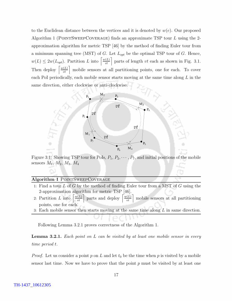
to the Euclidean distance between the vertices and it is denoted by w(e). Our proposed
Algorithm 1 (PointSweepCoverage) finds an approximate TSP tour L using the 2-
approximation algorithm for metric TSP [46] by the method of finding Euler tour from
a minimum spanning tree (MST) of G. Let Lopt be the optimal TSP tour of G. Hence,
w(L) ≤ 2w(Lopt). Partition L into⌈
w(L)vt
⌉
parts of length vt each as shown in Fig. 3.1.
Then deploy⌈
w(L)vt
⌉
mobile sensors at all partitioning points, one for each. To cover
each PoI periodically, each mobile sensor starts moving at the same time along L in the
same direction, either clockwise or anti-clockwise.
vt
P
7P 5P
P 3 2P
P 1
M 3
M 4
2M
M 1
P 4
vt
vt
vt
6
Figure 3.1: Showing TSP tour for PoIs, P1, P2, · · · , P7, and initial positions of the mobilesensors M1, M2, M3, M4
Algorithm 1 PointSweepCoverage
1: Find a tour L of G by the method of finding Euler tour from a MST of G using the2-approximation algorithm for metric TSP [46].
2: Partition L into⌈
w(L)vt
⌉
parts and deploy⌈
w(L)vt
⌉
mobile sensors at all partitioning
points, one for each.3: Each mobile sensor then starts moving at the same time along L in same direction.
Following Lemma 3.2.1 proves correctness of the Algorithm 1.
Lemma 3.2.1. Each point on L can be visited by at least one mobile sensor in every
time period t.
Proof. Let us consider a point p on L and let t0 be the time when p is visited by a mobile
sensor last time. Now we have to prove that the point p must be visited by at least one
17
TH-1437_10612305

mobile sensor within t0 + t time. According to the deployment strategy of the mobile
sensors any two consecutive mobile sensors are within a distance of at most vt at any
time. So, when p is visited by a mobile sensor at t0, another mobile sensor was on the
way to p and within the distance of vt along L. Hence p will be again visited by another
mobile sensor within next t time.
Theorem 3.2.2. The number of mobile sensors required for the Algorithm 1 is no more
than twice the number needed for the optimal solution.
Proof. Let Lopt be the optimal TSP tour for the graph G. Let L be the tour calculated
by the Algorithm 1. Then by 2-approximation algorithm for metric TSP [46], w(L) ≤2w(Lopt). Let Nopt be the number of mobile sensors required for optimal solution. Then
Nopt × vt ≥ w(Lopt), i.e., Nopt ≥⌈
w(Lopt)vt
⌉
. Let N be the number of mobile sensors
calculated by Algorithm 1. Then N =⌈
w(L)vt
⌉
. Therefore, the approximation ratio of
the Algorithm 1 is equal to NNopt
≤⌈
2w(Lopt)vt
⌉/⌈
w(Lopt)vt
⌉
≤ 2.
Remark 3.2.3. The running time of Algorithm 1 is not polynomial. All the other steps
expect the partitioning of the tour L can be done in polynomial time. The MST of the
complete graph G can be computed in O(n2) time using Prim’s algorithm, where n is
the number of vertices of G. The edges of the MST can be doubled in O(n) time and the
Euler tour on it can be found in O(n) time [22]. The tour L can be computed in O(n)
time from the Euler tour. But computing the partitioning points on L will take O( Lvt)
time. Hence time complexity of Algorithm 1 is O(n2+ Lvt) which is not polynomial in n.
3.3 Sweep Coverage on a Weighted Graph
In this section, we propose solution for sweep coverage problem on a weighted undirected
graph. The vertices of the graph are considered as PoIs. The mobile sensors can move
along the edges of the graph with a uniform speed v. Let G = (U,E, w) be a weighted
graph, where weight of an edge (ui, uj) for ui, uj ∈ U is denoted by w(ui, uj). Let n be
the total number of vertices in G. For any subgraph H of G, we denote w(H) for the
sum of the edge weights of H . We define sweep coverage for the vertices of a graph as
follows.
18
TH-1437_10612305

Definition 3.3.1 (t-sweep coverage). Let U = {u1, u2, · · · , un} be the vertices of a
weighted graph G = (U,E, w), and M = {m1, m2, · · · , mn} be the set of mobile sensors.
The mobile sensors move with a uniform speed v along edges of the graph. A vertex
ui is said to be t-sweep covered if and only if at least one mobile sensor mj visits ui in
every t time period.
Problem 1 (Sweep coverage problem on graph). Let U = {u1, u2, · · · , un} be the
vertices of a weighted graph G = (U,E, w) and M = {m1, m2, · · · , mn} be the set of
mobile sensors. The mobile sensors move with a uniform speed v along the edges of the
graph. For a given t > 0, find the minimum number of mobile sensors such that each
vertex of G is t-sweep covered.
We propose Algorithm 2 (GraphSweepCoverage) to find minimum number of
mobile sensors for the sweep coverage problem on graph. From step 1 to step 11 of
the algorithm execute in n iterations for finding the best possible solution i.e., number
of mobile sensors. In kth iteration (1 ≤ k ≤ n), the minimum spanning forest Fk
with k connected components C1, C2, · · · , Ck is computed. After that k disjoint tours
T1, T2, · · · , Tk are found by doubling all edges of each component. Partition each Ti into⌈
w(Ti)vt
⌉
parts of weight at most vt. If Ti contains only one vertex, number of partition on
Ti is one. Total number of partitions for kth iteration denoted by Nk and which is equal
to the number of mobile sensors required for the iteration. Minimum over the number of
mobile sensors of all iterations is chosen as the output of Algorithm 2. Initial positions
and the movement schedule of the mobile sensors are calculated within step 13 to step
21 of the algorithm.
3.3.1 Analysis
Theorem 3.3.2. Algorithm 2 guarantees t-sweep coverage for each vertex of G.
Proof. For any vertex ui we want to show that it is t-sweep covered. According to
Algorithm 2, there are two following cases.
Case 1: (ui is in a component with more than one vertex) Let ui is visited by
a mobile sensor mj at time t0. According to the algorithm, mobile sensors are
19
TH-1437_10612305

Algorithm 2 GraphSweepCoverage
1: for k = 1 to n do2: Find the minimum spanning forest Fk on G with n− k edges. Let C1, C2, · · · , Ck
be the connected components of Fk.3: Nk = 0.4: for j = 1 to k do5: if Cj is a component having more than one vertex then
6: Nk = Nk +⌈
2w(Ci)vt
⌉
.
7: else8: Nk = Nk + 1.9: end if10: end for11: end for12: Let J be the index ∈ {1, 2, · · · , n} such that NJ = min{N1, N2, · · · , Nn}.13: Let C1, C2, · · · , CJ be the connected components of FJ .14: for i = 1 to J do15: if Cj is a component having more than one vertex then16: Find a Eulerian tour Ti on Ci by doubling each edge of Cj . Partition the tour
into⌈
w(Ti)vt
⌉
parts and deploy one mobile sensor at each of the partitioning
points.17: else18: Deploy one mobile sensor at the vertex of Ci.19: end if20: end for21: All mobile sensors start moving at the same time along the respective tours having
more than one vertex in same direction. If a mobile sensor is deployed on a tourcontaining only one vertex then it periodically monitors the vertex.
initially deployed within vt distance apart. Then the mobile sensors start moving
with same speed v in the same direction. So ui will be again visited by the next
mobile sensor of mj within time t+ t0.
Case 2: (ui is in a component with no other vertices) In this case the statement
of the theorem is trivially true as one mobile sensor is deployed at ui and which
periodically covers it.
Lemma 3.3.3. Let opt be the number of mobile sensors needed in the optimal solution.
Let opt′ be the minimum number of paths of weight ≤ vt which span U on G. Then
20
TH-1437_10612305

opt ≥ opt′.
Proof. We want to prove it by the method of contradiction. Let us assume opt < opt′.
Consider the paths of movements by the mobile sensors in the optimal solution during
any time period [t0, t0 + t]. Let P1, P2, · · · , Popt be the movement paths of the mobile
sensors with w(Pi) ≤ vt. Since each vertex is visited by a mobile sensor at least once
in time period t therefore⋃opt
i=1 Pi spans all the vertices of U . Hence, {P1, P2, · · · , Popt}is a collection of paths with w(Pi) ≤ vt that spans U , which contradicts the fact that
opt < opt′. Therefore opt ≥ opt′.
Theorem 3.3.4. The Algorithm 2 is a 3-approximation algorithm.
Proof. Let opt be the minimum number of mobile sensors required in the optimal solu-
tion. Let opt′ be the minimum number of paths of weight ≤ vt, which span U on G and
Min path be the sum of the weights of all such paths. Then by Lemma 3.3.3,
opt′ ≤ opt (3.3.1)
and
Min path ≤ opt′ × vt (3.3.2)
Again, these opt′ number of paths of weights ≤ vt forms a spanning forest with opt′
disjoint connected components. As Fopt′ is the minimum spanning forest with opt′ con-
nected components, therefore,
w(Fopt′) ≤ Min path. (3.3.3)
Algorithm 2 chooses the minimum over all Nk for k = 1 to n. Let us consider the
iteration of the algorithm when k = opt′. Consider a connected component Ci of Fk.
If Ci is a component with more than one vertex, then number of partitions on Ci is⌈
2w(Ci)vt
⌉
which is ≤(
2w(Ci)vt
+ 1)
. If Ci is a component with one vertex, then w(Ci) = 0
and number of partition on Ci is 1 which is equal to(
2w(Ci)vt
+ 1)
. Therefore, total
21
TH-1437_10612305

number of partitions in this iteration is given by,
Nk ≤k∑
i=1
(
2w(Ci)
vt+ 1
)
=2w(Fk)
vt+ k
≤ 2Min path
vt+ k from Equation (3.3.3)
≤ 2k + k from Equation (3.3.2)
= 3k
≤ 3opt from Equation (3.3.1)
Since N ≤ Nk, therefore, N ≤ 3opt. Therefore the approximation factor of the Algo-
rithm 2 is 3.
Theorem 3.3.5. The time complexity of Algorithm 2 is O(n2 logn).
Proof. Selection of first k edges of a graph in Kruskal’s algorithm gives the minimum
spanning forest with n− k components. For each k, depth first search can be applied to
identify the connected components. Hence time complexity for computing the step 1-13
is O(n2 log n + n2). In step 16, O(n) time is required to find partitioning points of the
Eulerian tours after doubling each of the components. Therefore overall time complexity
of the Algorithm 2 is O(n2 logn).
3.4 Sweep Coverage in Presence of Obstacles
A mobile sensor cannot move straight from a PoI ui to another PoI uj in presence of an
obstacle on the path. An alternative path is required to avoid the obstacle. To calculate
an alternative path between any pair of PoIs we use the idea of visibility graph [34, 58].
There is an edge between two vertices of a visibility graph if line joining the vertices
does not intersect any obstacle. For simplicity we assume obstacles are polygonal shape.
Position of the polygons and their vertices are known. The construction of the visibility
graph Gv for a given set of PoIs and obstacles is given below.
22
TH-1437_10612305
The vertex set of Gv is the union of PoIs and the vertices of all obstacles. There is an
edge between two vertices of Gv if they are visible to each other, i.e., no obstacle between
their line of sight path. The weight of an edge is Euclidean distance between respective
vertices. In presence of obstacles on the direct path of ui and uj, an alternative path
is calculated through the vertices of polygons to avoid collision with the obstacles. All
pair shortest path among the PoIs can be found on Gv using Floyd-Warshall algorithm.
We construct a complete graph G′ for the set of vertices corresponding to the set of PoIs
only with edge weight w, where w is defined as w(ui, uj) = length of the shortest path
between vertices ui and uj in Gv. Each edge (ui, uj) of G′ corresponds one path between
ui and uj in Gv. Apply Algorithm 2 on G′ to sweep cover the set of PoIs.
Theorem 3.4.1. The time complexity of Algorithm 2 is O((n + k)3), where n is the
number of PoIs and k is total number of vertices of the polygonal obstacles.
Proof. The total number of vertices of the visibility graph Gv is (n + k), since Gv is
constructed with all PoIs and vertices of the polygonal obstacles. The computation of
Gv can be done in O(n2k) time, since intersection of a line segment with an obsta-
cle can be found in O(k) time. All pair shortest paths for the PoIs can be found in
O(n + k)3 time using Floyd-Warshall algorithm. The running time of Algorithm 2 is
O ((n+ k)2 log(n+ k)). Hence when polygonal obstacles are present in the plane with
total k vertices, the time complexity of Algorithm 2 is O((n+ k)3).
3.5 Simulation
In this section, we study performance of our proposed Algorithm 1 for sweep coverage
problem through simulation. We compare Algorithm 1 with MinExpand algorithm pro-
posed by Du et al. [19]. The idea of the MinExpand algorithm is to find disjoint cycles
having subset of PoIs of length less than or equal to vt. Then, one mobile sensor is
assigned for one cycle to guarantee t-sweep coverage of the given set of PoIs. We im-
plement both of the algorithms, Algorithm 1 and MinExpand for comparison study. We
generate different set of PoIs randomly inside a 200 meter by 200 meter square region
in a two dimensional plane. The PoIs are the input for both of the above algorithms.
23
TH-1437_10612305
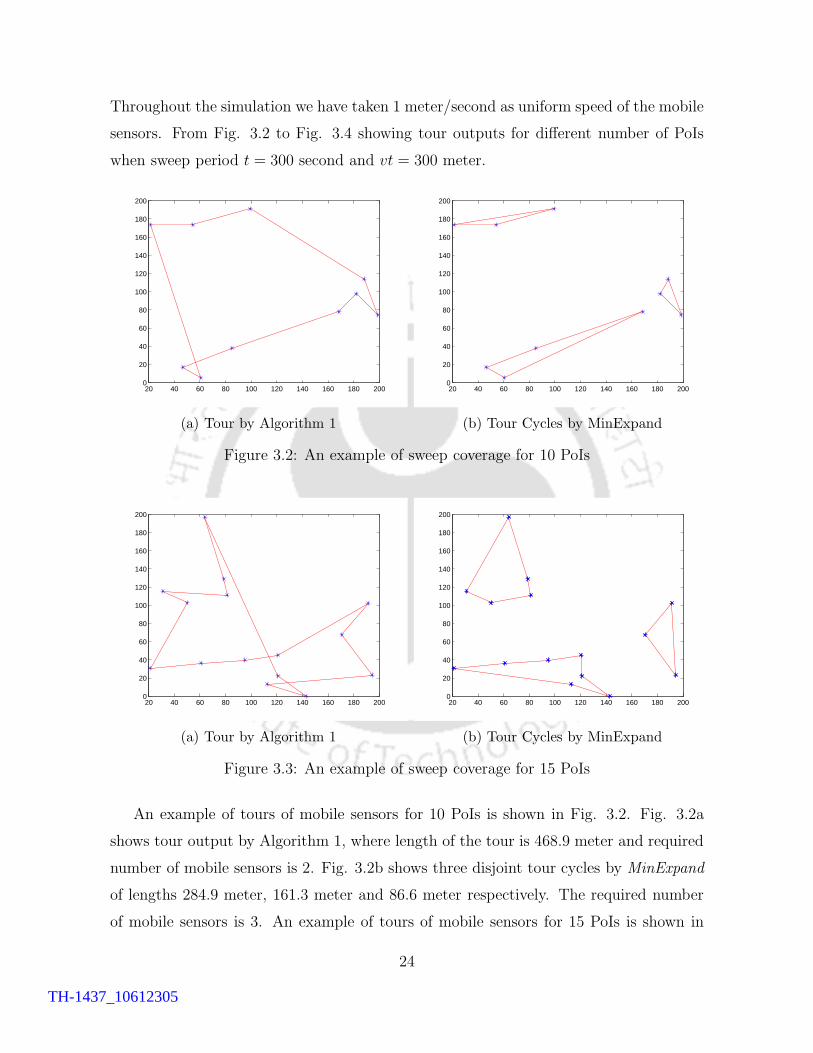
Throughout the simulation we have taken 1 meter/second as uniform speed of the mobile
sensors. From Fig. 3.2 to Fig. 3.4 showing tour outputs for different number of PoIs
when sweep period t = 300 second and vt = 300 meter.
20 40 60 80 100 120 140 160 180 2000
20
40
60
80
100
120
140
160
180
200
(a) Tour by Algorithm 1
20 40 60 80 100 120 140 160 180 2000
20
40
60
80
100
120
140
160
180
200
(b) Tour Cycles by MinExpand
Figure 3.2: An example of sweep coverage for 10 PoIs
20 40 60 80 100 120 140 160 180 2000
20
40
60
80
100
120
140
160
180
200
(a) Tour by Algorithm 1
20 40 60 80 100 120 140 160 180 2000
20
40
60
80
100
120
140
160
180
200
(b) Tour Cycles by MinExpand
Figure 3.3: An example of sweep coverage for 15 PoIs
An example of tours of mobile sensors for 10 PoIs is shown in Fig. 3.2. Fig. 3.2a
shows tour output by Algorithm 1, where length of the tour is 468.9 meter and required
number of mobile sensors is 2. Fig. 3.2b shows three disjoint tour cycles by MinExpand
of lengths 284.9 meter, 161.3 meter and 86.6 meter respectively. The required number
of mobile sensors is 3. An example of tours of mobile sensors for 15 PoIs is shown in
24
TH-1437_10612305
0 50 100 150 2000
20
40
60
80
100
120
140
160
180
200
(a) Tour by Algorithm 1
0 50 100 150 2000
20
40
60
80
100
120
140
160
180
200
(b) Tour Cycles by MinExpand
Figure 3.4: An example of sweep coverage for 20 PoIs
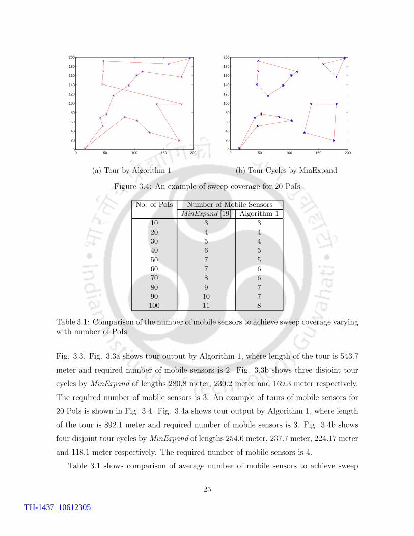
No. of PoIs Number of Mobile SensorsMinExpand [19] Algorithm 1
10 3 320 4 430 5 440 6 550 7 560 7 670 8 680 9 790 10 7100 11 8
Table 3.1: Comparison of the number of mobile sensors to achieve sweep coverage varyingwith number of PoIs
Fig. 3.3. Fig. 3.3a shows tour output by Algorithm 1, where length of the tour is 543.7
meter and required number of mobile sensors is 2. Fig. 3.3b shows three disjoint tour
cycles by MinExpand of lengths 280.8 meter, 230.2 meter and 169.3 meter respectively.
The required number of mobile sensors is 3. An example of tours of mobile sensors for
20 PoIs is shown in Fig. 3.4. Fig. 3.4a shows tour output by Algorithm 1, where length
of the tour is 892.1 meter and required number of mobile sensors is 3. Fig. 3.4b shows
four disjoint tour cycles by MinExpand of lengths 254.6 meter, 237.7 meter, 224.17 meter
and 118.1 meter respectively. The required number of mobile sensors is 4.
Table 3.1 shows comparison of average number of mobile sensors to achieve sweep
25
TH-1437_10612305
20 30 40 50 60 70 80 90 1003
4
5
6
7
8
9
10
11
Number of PoIs
Num
ber
of m
obile
sen
sors
Algorithm 1: PointSweepCoverageMinExpand
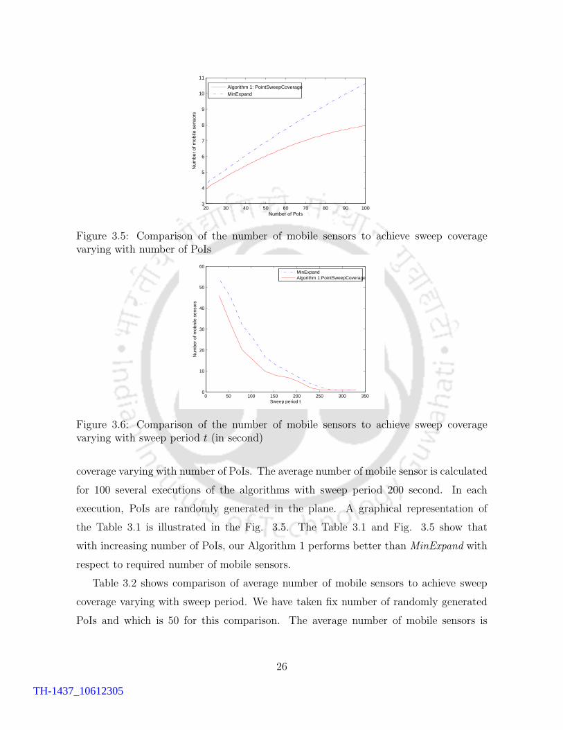
Figure 3.5: Comparison of the number of mobile sensors to achieve sweep coveragevarying with number of PoIs
0 50 100 150 200 250 300 3500
10
20
30
40
50
60
Sweep period t
Num
ber
of m
obni
le s
enso
rs
MinExpandAlgorithm 1:PointSweepCoverage
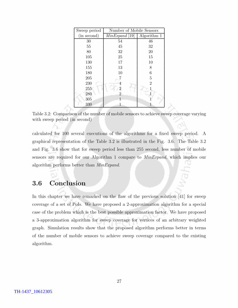
Figure 3.6: Comparison of the number of mobile sensors to achieve sweep coveragevarying with sweep period t (in second)
coverage varying with number of PoIs. The average number of mobile sensor is calculated
for 100 several executions of the algorithms with sweep period 200 second. In each
execution, PoIs are randomly generated in the plane. A graphical representation of
the Table 3.1 is illustrated in the Fig. 3.5. The Table 3.1 and Fig. 3.5 show that
with increasing number of PoIs, our Algorithm 1 performs better than MinExpand with
respect to required number of mobile sensors.
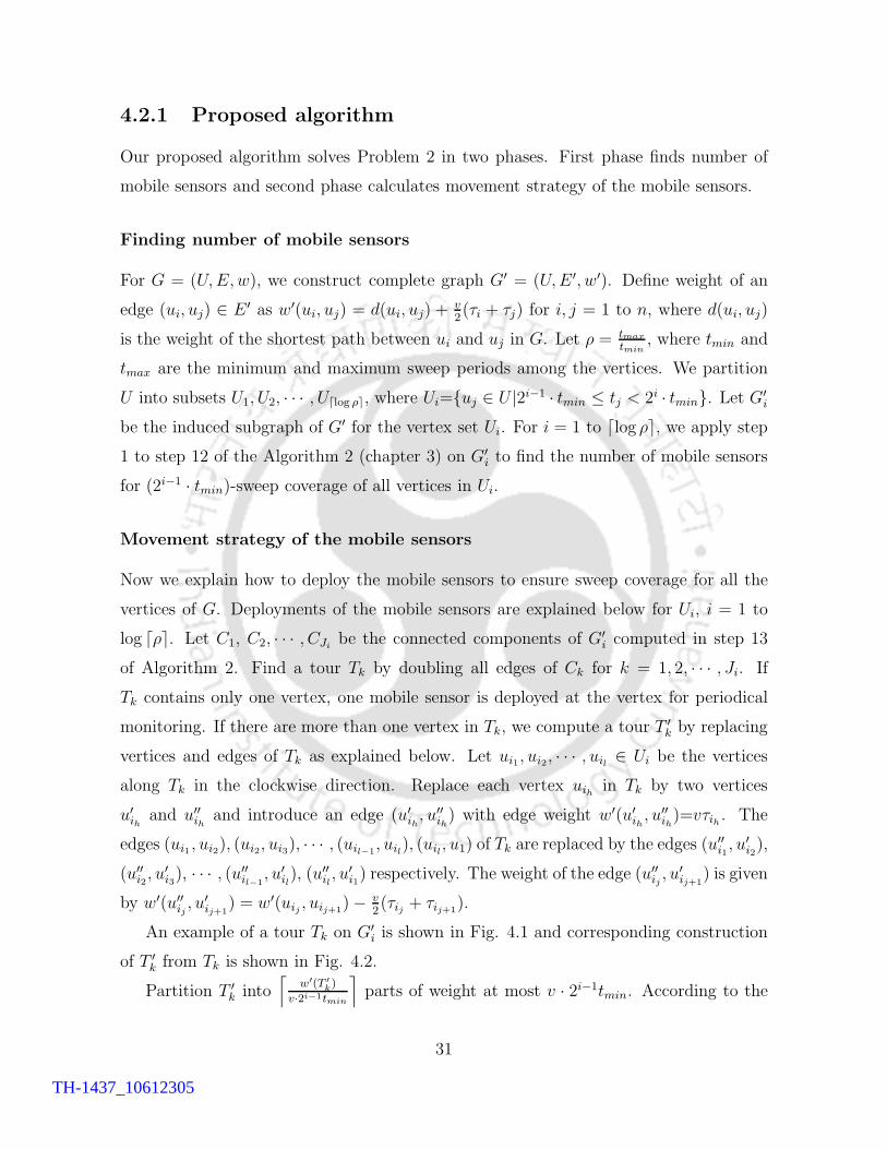
Table 3.2 shows comparison of average number of mobile sensors to achieve sweep
coverage varying with sweep period. We have taken fix number of randomly generated
PoIs and which is 50 for this comparison. The average number of mobile sensors is
26
TH-1437_10612305
Sweep period Number of Mobile Sensors(in second) MinExpand [19] Algorithm 1
30 54 4655 45 3280 32 20105 25 15130 17 10155 13 8180 10 6205 7 5230 4 2255 2 1280 2 1305 1 1330 1 1
Table 3.2: Comparison of the number of mobile sensors to achieve sweep coverage varyingwith sweep period (in second)
calculated for 100 several executions of the algorithms for a fixed sweep period. A
graphical representation of the Table 3.2 is illustrated in the Fig. 3.6. The Table 3.2
and Fig. 3.6 show that for sweep period less than 255 second, less number of mobile
sensors are required for our Algorithm 1 compare to MinExpand, which implies our
algorithm performs better than MinExpand.
3.6 Conclusion
In this chapter we have remarked on the flaw of the previous solution [41] for sweep
coverage of a set of PoIs. We have proposed a 2-approximation algorithm for a special
case of the problem which is the best possible approximation factor. We have proposed
a 3-approximation algorithm for sweep coverage for vertices of an arbitrary weighted
graph. Simulation results show that the proposed algorithm performs better in terms
of the number of mobile sensors to achieve sweep coverage compared to the existing
algorithm.
27
TH-1437_10612305

TH-1437_10612305

Chapter 4
Sweep Coverage with Heterogeneity
4.1 Introduction
In Chapter 3, we consider the sweep coverage problem where parameters are homoge-
neous i.e., sweep periods of all PoIs are same and speeds of all mobile sensors are also
same. But there are different applications where heterogeneity may present. For exam-
ple, monitoring machineries of an industry, where different machines may have different
importance. A few machines must be monitored more frequently than the others. So, in
terms of sweep coverage, sweep periods of all machines are not same. Similarly, mobile
sensors may not have same speed. In this chapter, we investigate two different sweep
coverage problems considering two different contexts of heterogeneity. In the first prob-
lem, sweep periods of the PoIs are different and in the second problem, the speeds of the
mobile sensors are different. In practice some processing time is required for a mobile
sensor to process some tasks such as monitoring, sampling or exchanging data at each of
the PoIs during its visit. Some finite amount of processing delays/times for the mobile
sensors at the PoIs are included in the first problem.
4.1.1 Contribution
In this chapter, our contributions are as follows:
• We propose an approximation algorithm to solve the sweep coverage problem for
a weighted graph when vertices of the graph have different sweep periods and
29
TH-1437_10612305

processing times. The approximation factor of the algorithm is O(log ρ), where
ρ = tmax
tmin, tmin and tmax are the minimum and maximum sweep periods among the
vertices.
• If speeds of the mobile sensors are different, we prove that it is impossible to design
any constant factor approximation algorithm to solve the sweep coverage problem,
unless P=NP.
4.2 Sweep Coverage with Different Sweep Periods
and Processing Times
Definition of the sweep coverage [41] for different sweep periods of the PoIs is given
below.
Definition 4.2.1. Let U = {u1, u2, · · · , un} be a set of PoIs, and {t1, t2, · · · , tn} be the
set of sweep periods. Let M = {m1, m2, · · · , mn} be the set of mobile sensors which can
move with a uniform speed v. A PoI ui is said to be ti-sweep covered iff a mobile sensor
visits ui at least once in every ti time period.
The objective of the sweep coverage problem is to find minimum number of mobile
sensor such that each ui is ti sweep covered. Li et al. [41] proposed a 3-approximation
algorithm for the problem. But there is a serious flaw in the algorithm. The flaw can
be shown by the same example described in the introduction of the previous Chapter
3. Here we propose an algorithm to solve the sweep coverage problem called DSSweep
coverage problem, where sweep periods for the vertices of a weighted graph are different.
The vertices of the graph are considered as the set of PoIs. The mobile sensors use some
finite amount of processing time during their visit at each of the vertices.
Problem 2 (DSSweep Coverage Problem). Let U = {u1, u2, · · · , un} be the vertex set
of a weighted graph G = (U,E, w). Let ti and τi be the sweep period and processing
time for ui, respectively for i = 1, · · · , n. Let M = {m1, m2, · · · , mn} be the set of
mobile sensors which can move with a uniform speed v along the edges of the graph.
Find the minimum number of mobile sensors such that each ui is ti-sweep covered.
30
TH-1437_10612305
4.2.1 Proposed algorithm
Our proposed algorithm solves Problem 2 in two phases. First phase finds number of
mobile sensors and second phase calculates movement strategy of the mobile sensors.
Finding number of mobile sensors
For G = (U,E, w), we construct complete graph G′ = (U,E ′, w′). Define weight of an
edge (ui, uj) ∈ E ′ as w′(ui, uj) = d(ui, uj) +v2(τi + τj) for i, j = 1 to n, where d(ui, uj)
is the weight of the shortest path between ui and uj in G. Let ρ = tmax
tmin, where tmin and
tmax are the minimum and maximum sweep periods among the vertices. We partition
U into subsets U1, U2, · · · , Udlog ρe, where Ui={uj ∈ U |2i−1 · tmin ≤ tj < 2i · tmin}. Let G′i
be the induced subgraph of G′ for the vertex set Ui. For i = 1 to dlog ρe, we apply step
1 to step 12 of the Algorithm 2 (chapter 3) on G′i to find the number of mobile sensors
for (2i−1 · tmin)-sweep coverage of all vertices in Ui.
Movement strategy of the mobile sensors
Now we explain how to deploy the mobile sensors to ensure sweep coverage for all the
vertices of G. Deployments of the mobile sensors are explained below for Ui, i = 1 to
log dρe. Let C1, C2, · · · , CJi be the connected components of G′i computed in step 13
of Algorithm 2. Find a tour Tk by doubling all edges of Ck for k = 1, 2, · · · , Ji. If
Tk contains only one vertex, one mobile sensor is deployed at the vertex for periodical
monitoring. If there are more than one vertex in Tk, we compute a tour T ′k by replacing
vertices and edges of Tk as explained below. Let ui1, ui2, · · · , uil ∈ Ui be the vertices
along Tk in the clockwise direction. Replace each vertex uih in Tk by two vertices
u′ih
and u′′ih
and introduce an edge (u′ih, u′′
ih) with edge weight w′(u′
ih, u′′
ih)=vτih . The
edges (ui1 , ui2), (ui2, ui3), · · · , (uil−1, uil), (uil, u1) of Tk are replaced by the edges (u′′
i1, u′
i2),
(u′′i2, u′
i3), · · · , (u′′
il−1, u′
il), (u′′
il, u′
i1) respectively. The weight of the edge (u′′
ij, u′
ij+1) is given
by w′(u′′ij, u′
ij+1) = w′(uij , uij+1
)− v2(τij + τij+1
).
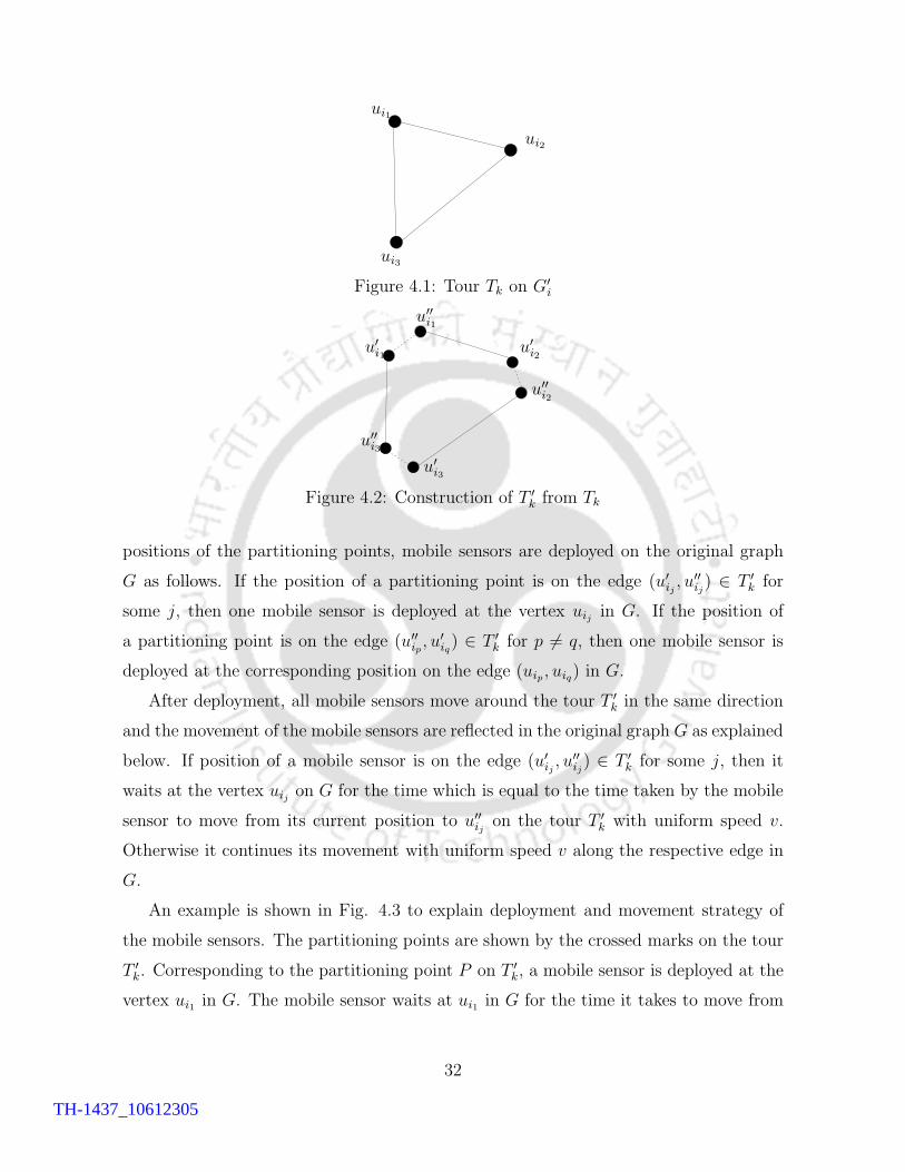
An example of a tour Tk on G′i is shown in Fig. 4.1 and corresponding construction
of T ′k from Tk is shown in Fig. 4.2.
Partition T ′k into
⌈
w′(T ′k)
v·2i−1tmin
⌉
parts of weight at most v · 2i−1tmin. According to the
31
TH-1437_10612305
ui3
ui2
ui1
Figure 4.1: Tour Tk on G′i
u′i1
u′′i1
u′i2
u′′i2
u′i3
u′′i3
Figure 4.2: Construction of T ′k from Tk
positions of the partitioning points, mobile sensors are deployed on the original graph
G as follows. If the position of a partitioning point is on the edge (u′ij, u′′
ij) ∈ T ′
k for
some j, then one mobile sensor is deployed at the vertex uij in G. If the position of
a partitioning point is on the edge (u′′ip, u′
iq) ∈ T ′
k for p 6= q, then one mobile sensor is
deployed at the corresponding position on the edge (uip, uiq) in G.
After deployment, all mobile sensors move around the tour T ′k in the same direction
and the movement of the mobile sensors are reflected in the original graph G as explained
below. If position of a mobile sensor is on the edge (u′ij, u′′
ij) ∈ T ′
k for some j, then it
waits at the vertex uij on G for the time which is equal to the time taken by the mobile
sensor to move from its current position to u′′ij
on the tour T ′k with uniform speed v.
Otherwise it continues its movement with uniform speed v along the respective edge in
G.
An example is shown in Fig. 4.3 to explain deployment and movement strategy of
the mobile sensors. The partitioning points are shown by the crossed marks on the tour
T ′k. Corresponding to the partitioning point P on T ′
k, a mobile sensor is deployed at the
vertex ui1 in G. The mobile sensor waits at ui1 in G for the time it takes to move from
32
TH-1437_10612305
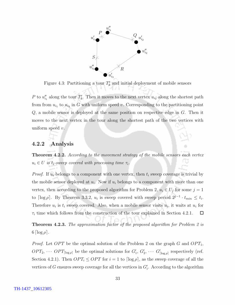
PQ
R
S
u′i1
u′′i1
u′i2
u′′i2
u′i3
u′′i3
Figure 4.3: Partitioning a tour T ′k and initial deployment of mobile sensors
P to u′′i1along the tour T ′
k. Then it moves to the next vertex ui2 along the shortest path
from from ui1 to ui2 in G with uniform speed v. Corresponding to the partitioning point
Q, a mobile sensor is deployed at the same position on respective edge in G. Then it
moves to the next vertex in the tour along the shortest path of the two vertices with
uniform speed v.
4.2.2 Analysis
Theorem 4.2.2. According to the movement strategy of the mobile sensors each vertex
ui ∈ U is ti-sweep covered with processing time τi.
Proof. If ui belongs to a component with one vertex, then ti sweep coverage is trivial by
the mobile sensor deployed at ui. Now if ui belongs to a component with more than one
vertex, then according to the proposed algorithm for Problem 2, ui ∈ Uj for some j = 1
to dlog ρe. By Theorem 3.3.2, ui is sweep covered with sweep period 2j−1 · tmin ≤ ti.
Therefore ui is ti sweep covered. Also, when a mobile sensor visits ui, it waits at ui for
τi time which follows from the construction of the tour explained in Section 4.2.1.
Theorem 4.2.3. The approximation factor of the proposed algorithm for Problem 2 is
6 dlog ρe.
Proof. Let OPT be the optimal solution of the Problem 2 on the graph G and OPT1,
OPT2, · · · OPTdlog ρe be the optimal solutions for G′1, G
′2, · · · G′
dlog ρe respectively (ref.
Section 4.2.1). Then OPTi ≤ OPT for i = 1 to dlog ρe, as the sweep coverage of all the
vertices of G ensures sweep coverage for all the vertices in G′i. According to the algorithm
33
TH-1437_10612305

for Problem 2 let OUT1, OUT2, · · · , OUTdlog ρe be the number of mobile sensors for G′1,
G′2, · · · G′
dlog ρe respectively. Then OUTi ≤ 6OPTi, as the length of the partition in
OPTi is at most twice of the length of the partition in OUTi and the Algorithm 2 is a
3-approximation algorithm. Hence, total number of mobile sensors needed is equals to∑dlog ρe
j=1 OUTj ≤ 6∑dlog ρe
j=1 OPTj ≤ 6 dlog ρeOPT . Therefore, the algorithm for Problem
2 is 6 dlog ρe-approximation algorithm.
Theorem 4.2.4. The running time of the algorithm for Problem 2 is O(n2 logn log ρ).
Proof. The time complexity of the Algorithm 2 is O(n2 log n). The algorithm for Prob-
lem 2 uses the Algorithm 2 as a subroutine for O(log ρ) disjoint set of of vertices. Hence
the running time is O(n2 logn log ρ).
Remark 4.2.5. Although it seems that the time complexity of the algorithm for Problem
2 is pseudo polynomial but according to the decomposition strategy of the vertices of
the graph there can be at most n non-empty disjoint vertex sets. Hence the complexity
of the algorithm is O(n3 log n) which is polynomial in n.
4.3 Inapproximability of Sweep Coverage with Mo-
bile Sensors having Different Speeds
In this section, we consider the sweep coverage problem called DVSweep coverage prob-
lem, where speeds of the mobile sensors may be different. Let m1, m2, · · · , mn be the
mobile sensors and v1, v2, · · · vn be their respective speeds, where vi ≥ 0 for all i= 1 to
n. The problem is to find minimum number of mobile sensors such that every vertex of
a given graph G is t-sweep covered.
Problem 3 (DVSweep Coverage Problem). Let U = {u1, u2, · · · , un} be the vertex
set of a weighted graph G = (U,E, w). Let m1, m2, · · · , mn be the mobile sensors and
v1, v2, · · · vn be their respective speeds, where vi ≥ 0 for all i= 1 to n. For a given t > 0,
find minimum number of mobile sensors such that each ui is t-sweep covered.
We prove that no polynomial time constant factor approximation algorithm exists
for the above problem, unless P=NP.
34
TH-1437_10612305
Theorem 4.3.1. No polynomial time constant factor approximation algorithm exists to
solve the sweep coverage problem by mobile sensors with different speeds, unless P=NP.
Proof. We prove the theorem by the method of contradiction. For the purpose, we
propose a polynomial time reduction from metric TSP problem, which is known to be
NP-hard, to an instance of Problem 3.
Suppose there exists a k-approximation algorithm A for Problem 3. Without loss of
generality we assume k is a positive integer. We consider an instance (G1, L) of metric
TSP, where G1 = (U1, E1, w1) is a complete weighted graph with n (> k) vertices and
weights of the edges of G1 are integer and satisfy triangle inequality. We construct a
complete graph G2 = (U2, E2, w2) with n2 vertices from G1 as follows. For each vertex
ui ∈ U1, we consider n vertices u1i , u
2i , · · ·un
i in U2 for i = 1, 2, · · · , n. We define weight
of an edge (uli, u
kj ) ∈ E2 as w2(u
li, u
kj ) = w1(ui, uj) − 1
(n+1)2for i 6= j and w2(u
li, u
ki ) =
1(n−1)(n+1)2
of G2.
Next, we prove that the graph G1 has a tour with weight at most l iff G2 has a
tour with weight at most l. To prove this, let T1 : ui1, ui2, · · · , uin, ui1 be a tour in
G1 having weight at most l, i.e., w1(T1) ≤ l. Now, we compute a tour T2 on G2 as
u1i1, u2
i1, · · · , un
i1, u1
i2, u2
i2, · · · , un
i2, · · · , u1
in, u2
in, · · · , un
in, u1
i1. The weight of T2 i.e., w2(T2)
is equal to∑n
i=1
∑n−1j=1 w2(u
ji , u
j+1i ) + w1(T1)− n
(n+1)2≤ n
(n+1)2+ l − n
(n+1)2= l.
Conversely, let T ′2 : x1, x2, · · · , xn2, x1 be a tour in G2 of weight at most l, where
x1, x2, · · · , xn2 ∈ U2 are distinct vertices. We construct a tour T ′1 from T ′
2 as follows.
First we remove all the edges of type (uki , u
li) from T ′
2. The remaining all edges of T ′2
are of the form (uki , u
lj) for i 6= j. For each and every such edge (uk
i , ulj) of T ′
2 we
consider corresponding edge (ui, uj) in G1 and construct a graph E . For example, if
edges (uk1i , ul1
j ) and (uk2i , ul2
j ) for k1 6= k2 and l1 6= l2 are in T ′2, then we consider the edge
(ui, uj) twice in E . One can easily verify that the graph E with all vertices U1 form an
Eulerian graph. We construct a tour T ′1 on G1 by short cutting the edges of E . Since the
edge weights of G1 follow triangle inequality, w1(T′1) ≤ w1(E) ≤ w2(T
′2) +
n2
(n+1)2< l+ 1.
Therefore, w1(T′1) ≤ l as edge weights in G1 are integers.
We consider an instance of the sweep coverage problem by mobile sensors with dif-
ferent speeds as follows: We take G2 as the input graph, sweep period t = 1, and a set of
n2 mobile sensors, among them speed of one mobile sensor is L and speeds of remaining
35
TH-1437_10612305

n2− 1 mobile sensors are zero. Let y be the number of mobile sensors returned by A on
G2.
Case 1: (y ≤ k) Among the k mobile sensors, speed of one mobile sensor is L and
speeds of remaining y − 1 mobile sensors are zero. Therefore, the mobile sensor
with speed L moves along a tour covering n2 − y + 1 vertices and remaining y − 1
mobile sensors cover remaining y − 1 vertices one for each. Since n > k therefore
n2−y+1 > n2−n. Hence at least one vertex from each of the set {u1i , u
2i , · · · , un
i }for different i is visited by the mobile sensor with speed L and weight of the tour is
at most L. From this tour, a tour T of weight at most L of G1 can be constructed
in the same way by constructing an Eulerian graph of G1 and short cutting as
explained before. Hence there is a tour on G1 with weight at most L that covers
all the vertices of G1.
Case 2: (y > k) As A is a k-approximation algorithm, we can say that there is no tour
on G2 with weight at most L that covers all the vertices of G2. This implies that
there is no tour on G1 with weight at most L that covers all the vertices of G1.
Hence, TSP can be decided in polynomial time by applying A on G2, which is a contra-
diction, unless P=NP. Hence the statement of the theorem follows.
4.4 Conclusion
In this chapter, we have discussed the sweep coverage problem with two different context
of heterogeneity. In the first problem, the sweep periods of the PoIs are different. We
have remarked on the flaw of the previous solution [41] of the problem. Our proposed
algorithm achieves approximation factor O(log ρ), where ρ = tmax
tmin, tmin and tmax are the
minimum and maximum sweep periods among the vertices. For the second problem, the
speeds of the mobile sensors are different. For this problem, we have proved that it is
impossible to design any constant factor approximation algorithm, unless P=NP.
36
TH-1437_10612305

Chapter 5
Solving Energy Issues for Sweep
Coverage
5.1 Introduction
Energy is a very important resource which is needed to be considered while designing
efficient algorithms for WSNs. Since the sensors have limited battery as energy source,
proper energy utilization can extend their lifetime. In this chapter, we consider an energy
efficient sweep coverage problem with mobile and static sensors by minimizing the total
energy utilization. Activity of a sensor is restricted by the capacity of its battery unless
the battery is recharged or replaced. It is also recommendable to recharge or replace the
battery just before (at a limiting condition) exceeding its capacity for optimal resource
utilization. It may happen that during some activities of a mobile sensor, capacity
of its battery is at the limiting condition. In that case the sensor stops its activities
until the battery is recharged or replaced. So, with the restriction on the maximum
energy utilization, how to guarantee sweep coverage with minimum number of mobile
sensors is a challenging problem. In this chapter we consider an energy restricted sweep
coverage problem where the total energy used by a mobile sensor in a given time period
is bounded.
37
TH-1437_10612305

5.1.1 Contribution
In this chapter, our contributions are as follows:
• We propose a variation of sweep coverage problem, called energy efficient sweep
coverage problem or ESweep coverage problem. The problem is NP-hard and
cannot be approximated within a factor of 2, unless P=NP. We propose an 8-
approximation algorithm to solve it.
• A 2-approximation algorithm is proposed for a special case of the above problem,
which is the best possible approximation factor.
• We introduce another variation of sweep coverage, called energy restricted sweep
coverage problem or ERSweep coverage problem and propose a (5+ 2α)-approximation
algorithm to solve this NP-hard problem.
5.2 Energy Efficient Sweep Coverage Problem
Instead of using mobile sensors, sometimes using both static and mobile sensors for sweep
coverage can be more efficient. For example, let us consider the scenario where there
are three points u1, u2, u3 in a plane. The distance between the points are as follows:
d(u1, u2) = 5, d(u2, u3) = 20, d(u3, u1) = 20. Let the value of vt is 10. According to
Algorithm 2 in Chapter 3, a mobile sensor is deployed to visit u1 and u2 and another
mobile sensor is deployed at u3. Now, since energy utilization of a static sensor is much
lesser than that of a mobile sensor, using one static sensor at u3 is more effective than
the use of a mobile sensor. Motivated by the above example, we redefine the sweep
coverage problem as follows.
Definition 5.2.1 (t-GSweep coverage). Let U = {u1, u2, · · · , un} be a set of PoIs,
S = {s1, s2, · · · , sn} be a set of static sensors and M = {m1, m2, · · · , mn} be a set of
mobile sensors. Let v be the uniform speed of the mobile sensors. For a given time
period t ≥ 0, a PoI ui is said to be t-GSweep covered if and only if either of the following
two cases happens:
1. A static sensor sj is deployed at ui which continuously monitors ui.
38
TH-1437_10612305

2. At least one mobile sensor mj visits ui in every t time period.
The time period t is called the sweep period of the set of points U .We define the following problem, called energy efficient sweep coverage problem, in
short ESweep coverage problem.
Problem 4 (ESweep Coverage Problem). Let U={u1, u2, · · · , un} be a set of PoIs,
S = {s1, s2, · · · , sp} be a set of static sensors and M = {m1, m2, · · · , mq} be a set of
mobile sensors. Let v be the uniform speed of the mobile sensors, λ, µ be the energy
consumptions per unit time by a static and a mobile sensors, respectively. For given
t > 0, find number of sensors, combination of static and mobile sensors such that t-
GSweep coverage of the set of PoIs can be guaranteed and total energy consumption per
unit of time is minimized.
The following theorem gives the complexity result for the ESweep coverage problem.
Theorem 5.2.2. The ESweep coverage problem is NP-hard and cannot be approximated
within a factor of 2, unless P=NP.
Proof. For λ = µ, the ESweep coverage problem reduces to the sweep coverage problem
presented in [41], where the objective is to minimize total number of sensors. According
to Theorem 1 in [41], the sweep coverage problem is NP-hard and cannot be approxi-
mated within a factor of 2 unless P = NP . Therefore, ESweep coverage problem is also
NP-hard and cannot be approximated within a factor of 2, unless P=NP.
To get the solution to ESweep coverage problem, we use solutions of k-TSP [25] and
k-MST [25, 48] problems.
Definition 5.2.3 (k-MST problem [25]). Let G = (V,E, w) be a weighed graph, where
the edge weights are positive real numbers and k be a given positive integer. Find a
minimum weighted tree of G that spans any k vertices of G.
Definition 5.2.4 (k-TSP problem [25]). Let G = (V,E, w) be a weighed graph, where
the edge weights are positive real numbers and k be a given positive integer. Find a
minimum weighted tour of G visiting any k vertices of G.
39
TH-1437_10612305
Both of the above problems are NP-hard and the best known solutions for these
problems are proposed by Garg in [25] where 2-approximation algorithms for both of
the problems are provided.
5.2.1 Algorithm and Analysis
In this section, we propose an approximation algorithm for the ESweep coverage problem
with approximation factor 8. Our algorithm use the 2-approximation algorithm for k-
MST [25] as a subroutine. Consider a set of PoIs U={u1, u2, · · · , un} in two dimensional
plane. Let G = (U,E, w) be the complete weighted graph with each PoI as a vertex and
the line segment joining two PoIs in the plane as edge. The weight of an edge e ∈ E
is equal to the Euclidean distance between the vertices and it is denoted by w(e). For
any subgraph H of G, we denote w(H) as the sum of the edge weights of H . We denote
V (H) and E(H) as the vertex and edge set of H respectively.
The inputs of the proposed Algorithm 3 (ESweepCoverage) are the graph G,
speed v, sweep period t, energy consumption per unit time for static and mobile senors
λ and µ, respectively. Output of the algorithm is the number of mobile and static
sensors with the deployment locations for static sensors and movement schedule for
mobile sensors. The formal description of the algorithm is as follows. At the beginning
of the algorithm a graph G′ = (U,E, w′) from G = (U,E, w) is constructed by changing
weight of every edge e ∈ E as follows. For all e ∈ E, if w(e) ≤ vt then assign w′(e) = w(e)vt
,
otherwise assign w′(e) = 1. Next, for each k, 1 ≤ k ≤ n, we do the following steps.
We compute a treeMSTG′
k which spans any k vertices ofG′ using the 2-approximation
algorithm [25] for k-MST. Let MSTGk be the corresponding tree of MSTG′
k in G. Now,
we delete all the edges of weight more than vt from MSTGk . This may split MSTG
k
into several connected components. Find tours on each of the components by doubling
the edges and short cutting. Then partition the tours into several parts of length vt.
Compute the value of fk = (λ · t)Xk + (µ · t)Yk, where Yk is the total number of parti-
tions over all tours and Xk = n − k. Let k = k0 for which the value of fk, 1 ≤ k ≤ n,
be minimum. We select the number of static sensors X = Xk0 and number of mobile
sensors Y = Yk0 as the output of our algorithm. The deployment locations of static
40
TH-1437_10612305

sensors and the movement schedules of mobile sensors are calculated as follows. There
are n−k0 vertices, which are not covered by MSTGk0, so n−k0 static sensors are deployed
at n− k0 vertices, one for each. For deployment of mobile sensors, assume that MSTGk0
is split into h components C1, C2, · · · , Ch. Let T1, T2, · · · , Th be the corresponding tours
on the components after doubling the edges and short cutting. For each j, 1 ≤ j ≤ h,
partition the tour Tj into⌈
w(Tj)
vt
⌉
parts of weight at most vt. Then deploy one mobile
sensor at each of the partitioning points on Tj. All mobile sensors deployed on Tj start
their movements along Tj at the same time in the same direction.
Algorithm 3 ESweepCoverage
1: Construct graph G′ = (U,E, w′) from G = (U,E, w)2: for k = 1 to n do3: Find a tree MSTG′
k which spans any k vertices of G′ using the 2-approximationalgorithm for k-MST [25] .
4: Remove all the edges with weight > vt from MSTGk . Assume that after removal
of the edges MSTGk is split into kc components C1, C2, · · · , Ckc.
5: Find tours T1, T2, · · · , Tkc by doubling the edges of each of the respective compo-nents and short cutting.
6: Set Yk=∑kc
i=1
⌈
w(Ti)vt
⌉
and Xk = n− k then define fk = (λ · t)Xk + (µ · t)Yk.
7: end for8: f = min{f1, f2, · · · , fk} and k0 is the index such that f = fk0 .
9: For k = k0 partition T1, T2, · · ·Th into∑h
i=1
⌈
w(Ti)vt
⌉
parts of weight vt (found in step
5).10: Deploy one mobile sensor at each of the partitioning points of every tour and deploy
one static sensor at each of the remaining n− k0 vertices.11: The mobile sensors start their movements at the same time along the corresponding
tours in the same direction.
Theorem 5.2.5. Algorithm 3 ensures t-GSweep coverage for each of the PoIs.
Proof. To prove it we consider any vertex ui and show that it is t-GSweep covered.
According to the Algorithm 3, either of the following two cases happens for ui.
Case 1. One static sensor is deployed at ui. In this case the statement is trivially true.
Case 2. ui is visited by some mobile sensors. Let ui is visited by a mobile sensor at time
t0. According to the algorithm, the mobile sensors are deployed within distance at most
vt along the tour in which ui belongs. So ui will be visited by the next mobile sensor
within time t+ t0.
41
TH-1437_10612305
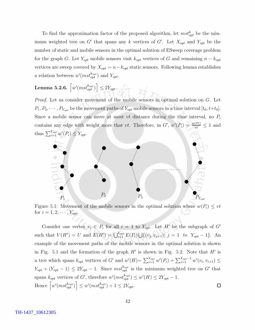
To find the approximation factor of the proposed algorithm, let mstkopt be the min-
imum weighted tree on G′ that spans any k vertices of G′. Let Xopt and Yopt be the
number of static and mobile sensors in the optimal solution of ESweep coverage problem
for the graph G. Let Yopt mobile sensors visit kopt vertices of G and remaining n− kopt
vertices are sweep covered by Xopt = n−kopt static sensors. Following lemma establishes
a relation between w′(mstkoptopt ) and Yopt.
Lemma 5.2.6.⌈
w′(mstkoptopt )
⌉
≤ 2Yopt.
Proof. Let us consider movement of the mobile sensors in optimal solution on G. Let
P1, P2, · · · , PYoptbe the movement paths of Yopt mobile sensors in a time interval [t0, t+t0].
Since a mobile sensor can move at most vt distance during the time interval, no Pi
contains any edge with weight more that vt. Therefore, in G′, w′(Pi) =w(Pi)vt
≤ 1 and
thus∑Yopt
i=1 w′(Pi) ≤ Yopt.
P1P2 P3 PYopt
Figure 5.1: Movement of the mobile sensors in the optimal solution where w(Pi) ≤ vt
for i = 1, 2, · · · , Yopt.
Consider one vertex vi ∈ Pi for all i = 1 to Yopt. Let H ′ be the subgraph of G′
such that V (H ′) = U and E(H ′) =⋃Yopt
i=1 E(Pi)⋃
{(vj, vj+1)| j = 1 to Yopt − 1}. An
example of the movement paths of the mobile sensors in the optimal solution is shown
in Fig. 5.1 and the formation of the graph H ′ is shown in Fig. 5.2. Note that H ′ is
a tree which spans kopt vertices of G′ and w′(H)=
∑Yopt
i=1 w′(Pi) +∑Yopt−1
i=1 w′(vi, vi+1) ≤Yopt + (Yopt − 1) ≤ 2Yopt − 1. Since mst
koptopt is the minimum weighted tree on G′ that
spans kopt vertices of G′, therefore w′(mst
koptopt ) ≤ w′(H) ≤ 2Yopt − 1.
Hence⌈
w′(mstkoptopt )
⌉
≤ w′(mstkoptopt ) + 1 ≤ 2Yopt.
42
TH-1437_10612305
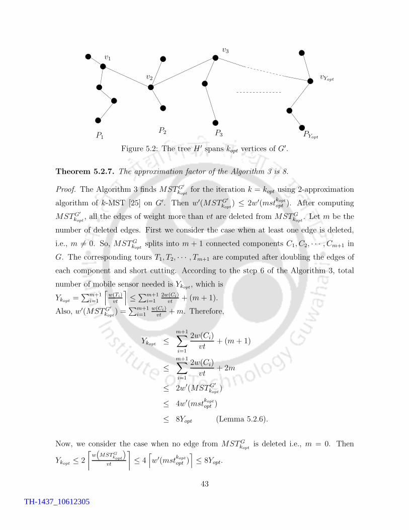
P1P2 P3 PYopt
v1
v2
v3
vYopt
Figure 5.2: The tree H ′ spans kopt vertices of G′.
Theorem 5.2.7. The approximation factor of the Algorithm 3 is 8.
Proof. The Algorithm 3 finds MSTG′
koptfor the iteration k = kopt using 2-approximation
algorithm of k-MST [25] on G′. Then w′(MSTG′
kopt) ≤ 2w′(mst
koptopt ). After computing
MSTG′
kopt, all the edges of weight more than vt are deleted from MSTG
kopt. Let m be the
number of deleted edges. First we consider the case when at least one edge is deleted,
i.e., m 6= 0. So, MSTGkopt
splits into m + 1 connected components C1, C2, · · · , Cm+1 in
G. The corresponding tours T1, T2, · · · , Tm+1 are computed after doubling the edges of
each component and short cutting. According to the step 6 of the Algorithm 3, total
number of mobile sensor needed is Ykopt, which is
Ykopt =∑m+1
i=1
⌈
w(Ti)vt
⌉
≤∑m+1
i=12w(Ci)
vt+ (m+ 1).
Also, w′(MSTG′
kopt) =
∑m+1i=1
w(Ci)vt
+m. Therefore,
Ykopt ≤m+1∑
i=1
2w(Ci)
vt+ (m+ 1)
≤m+1∑
i=1
2w(Ci)
vt+ 2m
≤ 2w′(MSTG′
kopt)
≤ 4w′(mstkoptopt )
≤ 8Yopt (Lemma 5.2.6).
Now, we consider the case when no edge from MSTGkopt
is deleted i.e., m = 0. Then
Ykopt ≤ 2
⌈
w(
MSTGkopt
)
vt
⌉
≤ 4⌈
w′(mstkoptopt )
⌉
≤ 8Yopt.
43
TH-1437_10612305

Therefore from the above two cases we have
λXkopt + µYkopt ≤ λXopt + 8µYopt ≤ 8(λXopt + µYopt). Hence, Algorithm 3 is an 8-
approximation algorithm.
5.2.2 A special case of ESweep coverage problem
A special case of the ESweep coverage problem is named as SESweep coverage problem,
which is presented in this section. In this special case all mobile sensors visit same subset
of PoIs to guarantee t-GSweep coverage while for the remaining PoIs, static sensors are
used to guarantee t-GSweep coverage. We define the SESweep coverage problem as
follows.
Problem 5 (SESweep Coverage Problem). Let U={u1, u2, · · · , un} be a set of PoIs,
S = {s1, s2, · · · , sp} be a set of static sensors and M = {m1, m2, · · · , mq} be a set
of mobile sensors. Let v be the uniform speed of the mobile sensors and λ and µ be
the energy consumption in every unit of time for a static sensor and mobile sensor,
respectively. Find X and Y , such that
1. X static sensors guarantee t-GSweep coverage of X PoIs,
2. remaining n−X PoIs are t-GSweep covered by Y mobile sensor such that each mobile
sensor visits all n−X PoIs and
3. λX + µY is minimum.
Note that the SESweep coverage problem is NP-hard and cannot be approximated
within a factor of 2, unless P=NP. The hardness proof follows from the proof of Theorem
1 in [41] for λ = µ. Algorithm 4 (SESweepCoverage) is proposed to solve the
SESweep coverage problem which uses the 2-approximation algorithm for k-TSP [25] as
a subroutine. The inputs of the Algorithm 4 are the graph G, speed v, sweep period t,
and energy consumption per unit time for static and mobile senors λ and µ, respectively.
Output of the algorithm is the number of mobile and static sensors with the deployment
locations for the static sensors and the movement schedule for the mobile sensors.
According to the Algorithm 4, all mobile sensors move along a single cycle which
cover a subset of PoIs of G. To cover the remaining PoIs, static sensors are deployed.
44
TH-1437_10612305
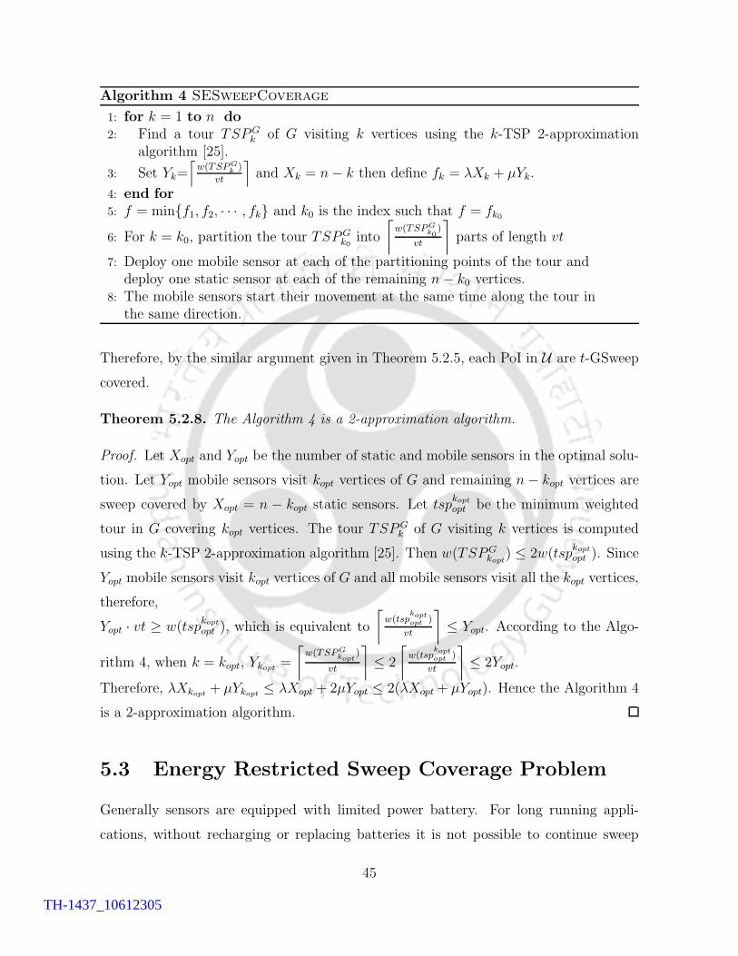
Algorithm 4 SESweepCoverage
1: for k = 1 to n do2: Find a tour TSPG
k of G visiting k vertices using the k-TSP 2-approximationalgorithm [25].
3: Set Yk=⌈
w(TSPGk)
vt
⌉
and Xk = n− k then define fk = λXk + µYk.
4: end for5: f = min{f1, f2, · · · , fk} and k0 is the index such that f = fk0
6: For k = k0, partition the tour TSPGk0
into
⌈
w(TSPGk0
)
vt
⌉
parts of length vt
7: Deploy one mobile sensor at each of the partitioning points of the tour anddeploy one static sensor at each of the remaining n− k0 vertices.
8: The mobile sensors start their movement at the same time along the tour inthe same direction.
Therefore, by the similar argument given in Theorem 5.2.5, each PoI in U are t-GSweep
covered.
Theorem 5.2.8. The Algorithm 4 is a 2-approximation algorithm.
Proof. Let Xopt and Yopt be the number of static and mobile sensors in the optimal solu-
tion. Let Yopt mobile sensors visit kopt vertices of G and remaining n− kopt vertices are
sweep covered by Xopt = n − kopt static sensors. Let tspkoptopt be the minimum weighted
tour in G covering kopt vertices. The tour TSPGk of G visiting k vertices is computed
using the k-TSP 2-approximation algorithm [25]. Then w(TSPGkopt
) ≤ 2w(tspkoptopt ). Since
Yopt mobile sensors visit kopt vertices of G and all mobile sensors visit all the kopt vertices,
therefore,
Yopt · vt ≥ w(tspkoptopt ), which is equivalent to
⌈
w(tspkoptopt )
vt
⌉
≤ Yopt. According to the Algo-
rithm 4, when k = kopt, Ykopt =
⌈
w(TSPGkopt
)
vt
⌉
≤ 2
⌈
w(tspkoptopt )
vt
⌉
≤ 2Yopt.
Therefore, λXkopt + µYkopt ≤ λXopt + 2µYopt ≤ 2(λXopt + µYopt). Hence the Algorithm 4
is a 2-approximation algorithm.
5.3 Energy Restricted Sweep Coverage Problem
Generally sensors are equipped with limited power battery. For long running appli-
cations, without recharging or replacing batteries it is not possible to continue sweep
45
TH-1437_10612305

coverage for long time. Also, it is not possible to recharge or replace batteries frequently.
After a certain time interval it can be done. Until then, the sensors have to use their
existing power of the batteries to continue activities. We introduce a variation of sweep
coverage problem, called Energy Restricted Sweep (ERSweep) coverage problem, where
there is an upper bound Z on the energy utilization by a mobile sensor for every time
period Γ. For example a mobile sensor consumes maximum energy Z in every time
period [Γ′ + kΓ,Γ′ + (k + 1)Γ], where Γ′ is the time when the mobile sensor starts its
movement and k ≥ 0. If a mobile sensor consumes Z energy before completing a time
period then it stops its activities until the forthcoming time period. Here activity means
movement and visiting the PoIs. The problem definition is given below.
Problem 6 (ERSweep Coverage Problem). Let U={u1, u2, · · · , un} be a set of PoIs
and M = {m1, m2, · · · , mq} be a set of mobile sensors. Let v be the uniform speed of
the mobile sensors and Z be the upper bound of the energy consumption by a mobile
sensor in every Γ time period. Let µi ≥ 0 be the energy consumption by a mobile sensor
to visit ui for i = 1 to n and µ be the energy consumption by a mobile sensor for its
movement per unit time. For a given t > 0, find the minimum number of mobile sensors
such that t-sweep coverage for every PoI in U is guaranteed.
If a mobile sensor has less than µi energy just before visiting ui, then it partially
completes the visit and wait until the starting of next time period.
Theorem 5.3.1. ERSweep Coverage Problem is NP-hard and cannot be approximated
within a factor of 2 unless P = NP .
Proof. In a particular case if there is no visiting cost at ui, i.e., µi = 0 for i = 1 to n
and t = Γ, µ · t = Z, the energy consumption by a mobile sensor in time t is Z, which
is the energy consumption due to its mobility. In this case the problem is equivalent to
find the minimum number of mobile sensors to guarantee sweep coverage for the set of
PoIs, which is NP-hard and cannot be approximated within a factor of 2, unless P=NP
according to Theorem 1 of [41]. Therefore, ERSweep Coverage Problem is NP-hard and
cannot be approximated within a factor of 2 unless P = NP .
46
TH-1437_10612305

5.3.1 Algorithm and Analysis
Let G = (U,E) be the complete weighted graph with each PoI as a vertex and the
line segment joining between two PoIs on the plane as an edge. We define two weight
functions w1 : E −→ R+ and w2 : E∪U −→ R
+ as follows. For any edge e = (ui, uj) ∈ E,
w1(e) = the Euclidean distance between ui and uj . For the edge e = (ui, uj) ∈ E,
w2(e) = w1(e)v
· µ and for each vertex ui ∈ U, w2(ui) = µi. For a subgraph H of G,
w1(H) =∑
e∈E(H)w1(e) and w2(H) =∑
v∈V (H)w2(v) +∑
e∈E(H)w2(e). Basically, for
any path P in G, w1(P ) gives the total distance a mobile sensor must travel to cover
each point on P and w2(P ) gives the total energy loss by a mobile sensor for moving
along P . The Algorithm 5 (ERSweepCoverage) is proposed to solve the ERSweep
coverage problem which returns the number of mobile sensors needed to guarantee t-
sweep coverage of the given set of PoIs by maintaining the energy restriction of the
mobile sensors.
Algorithm 5 ERSweepCoverage
1: for k = 1 to n do2: Find the minimum spanning forest Fk with k components on G with respect to
the weight function w1. Let C1, C2, · · ·Ck be the connected components of Fk.3: Find tours T1, T2, · · · , Tk by doubling the edges of C1, C2, · · ·Ck, respectively and
short cutting.4: for i = 1 to k do5: if Γ ≥ t then6: Set xi=PartitionTour1(Ti, t,Γ,Z)7: else8: Set xi=PartitionTour2(Ti, t,Γ,Z)9: end if10: end for11: Nk =
∑k
j=1 xj
12: end for13: N = min{N1, N2, · · · , Nn}, and let J be the index such that NJ = N
14: Repeat step 2 to step 11 for k = J .15: Deploy one mobile sensor at each of the partitioning points on each tour. The mobile
sensors start moving at the same time along the respective tours in same direction.
To find the best possible solution, from step 2 to step 11 of the Algorithm 5 is
executed in n iterations. In kth iteration (1 ≤ k ≤ n), the minimum spanning forest
Fk with k connected components with respect to w1 is computed. After that k disjoint
47
TH-1437_10612305
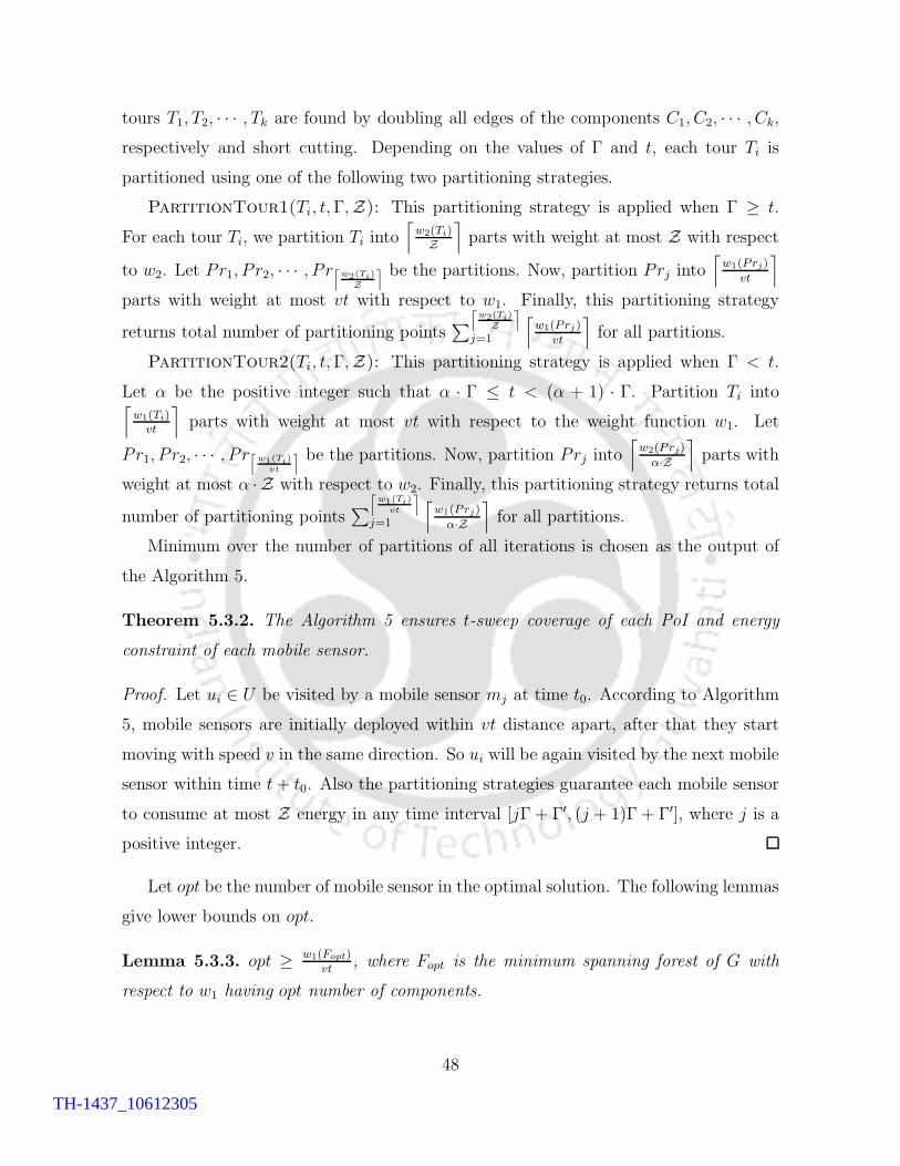
tours T1, T2, · · · , Tk are found by doubling all edges of the components C1, C2, · · · , Ck,
respectively and short cutting. Depending on the values of Γ and t, each tour Ti is
partitioned using one of the following two partitioning strategies.
PartitionTour1(Ti, t,Γ,Z): This partitioning strategy is applied when Γ ≥ t.
For each tour Ti, we partition Ti into⌈
w2(Ti)Z
⌉
parts with weight at most Z with respect
to w2. Let Pr1, P r2, · · · , P r⌈w2(Ti)
Z
⌉ be the partitions. Now, partition Prj into⌈
w1(Prj)
vt
⌉
parts with weight at most vt with respect to w1. Finally, this partitioning strategy
returns total number of partitioning points∑
⌈
w2(Ti)
Z
⌉
j=1
⌈
w1(Prj)
vt
⌉
for all partitions.
PartitionTour2(Ti, t,Γ,Z): This partitioning strategy is applied when Γ < t.
Let α be the positive integer such that α · Γ ≤ t < (α + 1) · Γ. Partition Ti into⌈
w1(Ti)vt
⌉
parts with weight at most vt with respect to the weight function w1. Let
Pr1, P r2, · · · , P r⌈w1(Ti)
vt
⌉ be the partitions. Now, partition Prj into⌈
w2(Prj)
α·Z
⌉
parts with
weight at most α · Z with respect to w2. Finally, this partitioning strategy returns total
number of partitioning points∑
⌈
w1(Ti)
vt
⌉
j=1
⌈
w1(Prj)
α·Z
⌉
for all partitions.
Minimum over the number of partitions of all iterations is chosen as the output of
the Algorithm 5.
Theorem 5.3.2. The Algorithm 5 ensures t-sweep coverage of each PoI and energy
constraint of each mobile sensor.
Proof. Let ui ∈ U be visited by a mobile sensor mj at time t0. According to Algorithm
5, mobile sensors are initially deployed within vt distance apart, after that they start
moving with speed v in the same direction. So ui will be again visited by the next mobile
sensor within time t+ t0. Also the partitioning strategies guarantee each mobile sensor
to consume at most Z energy in any time interval [jΓ + Γ′, (j + 1)Γ + Γ′], where j is a
positive integer.
Let opt be the number of mobile sensor in the optimal solution. The following lemmas
give lower bounds on opt.
Lemma 5.3.3. opt ≥ w1(Fopt)vt
, where Fopt is the minimum spanning forest of G with
respect to w1 having opt number of components.
48
TH-1437_10612305

Proof. Consider movements of the mobile sensors in optimal solution during the time
interval [t0, t + t0]. Let P1, P2, · · · , Popt be the movement paths of the mobile sensors.
Then w1(Pi) ≤ vt. P1, P2, · · · , Popt form a forest with opt number of components that
spans all the vertices of G. Since Fopt is the minimum spanning forest with opt number
of components, opt · vt ≥ w1(Fopt), i.e., opt ≥ w1(Fopt)vt
.
Lemma 5.3.4. If Γ ≥ t then opt ≥ w2(Fopt)
Z .
Proof. Let P1, P2, · · · , Popt be the movement paths of the mobile sensors during the time
interval [t0, t+ t0]. Then, w2(Pi) ≤ Z for i = 1 to opt. Now,
w2(P1) + w2(P2) + · · ·+ w2(Popt) =
opt∑
i=1
∑
u∈V (Pi)
w2(u) +∑
e∈E(Pi)
w2(e)
=∑
u∈V (G)
w2(u) +∑
e∈E(⋃opt
i=1 Pi)
w2(e)
=∑
u∈V (G)
w2(u) +µ
v·
∑
e∈E(⋃opt
i=1 Pi)
w1(e)
≥∑
u∈V (G)
w2(u) +µ
v·∑
e∈E(Fopt)
w1(e)
= w2(Fopt).
Therefore, Z · opt ≥ w2(Fopt), i.e., opt ≥ w2(Fopt)Z .
Lemma 5.3.5. If Γ < t then opt ≥ w2(Fopt)(α+1)·Z , where α is the integer such that α ·Γ ≤ t <
(α + 1) · Γ.
Proof. Let P1, P2, · · · , Popt be the movement paths of the mobile sensors in the optimal
solution during the time interval [t0, t+ t0]. Since α · Γ ≤ t < (α+ 1) · Γ, the maximum
energy consumption by a mobile sensor for its activities in the time interval [t0, t+ t0] is
less than (α+ 1) · Z. Therefore, w2(Pi) ≤ (α+ 1) · Z, for i = 1 to opt. Again, from the
proof of Lemma 5.3.4, we have w2(P1) + w2(P2) + · · ·+ w2(Popt) ≥ w2(Fopt). Therefore,
(α + 1) · Z · opt ≥ w2(Fopt), i.e., opt ≥ w2(Fopt)
(α+1)·Z .
49
TH-1437_10612305

Lemma 5.3.6. The number of partition xi on the tour Ti is given by
xi ≤ w2(Ti)
Z +w1(Ti)
vt+ 1 if Γ ≥ t
≤ w2(Ti)
α · Z +w1(Ti)
vt+ 1 if Γ < t
Proof. For Γ ≥ t each tour Ti is partitioned into parts with weight ≤ Z with respect
to w2. Let Pr1, P r2, · · · , P r⌈w2(Ti)
Z
⌉ be the partitions with w2(Pri) ≤ Z. According to
PartitionTour1(Ti, t,Γ,Z), total number of partitions on Ti is
xi =∑
⌈
w2(Ti)
Z
⌉
j=1
⌈
w1(Prj)
vt
⌉
≤ ∑
⌈
w2(Ti)
Z
⌉
j=1w1(Prj)
vt+⌈
w2(Ti)Z
⌉
≤ w1(Ti)vt
+⌈
w2(Ti)Z
⌉
≤ w1(Ti)vt
+w2(Ti)
Z + 1.
For Γ < t each tour Ti is partitioned into parts with weight ≤ vt with respect to
w1. Let Pr1, P r2, · · · , P r⌈w1(Ti)
vt
⌉ be the partitions with w1(Pri) ≤ vt. According to
PartitionTour2(Ti, t,Γ,Z), total number of partitions on Ti is
xi =∑
⌈
w1(Ti)
vt
⌉
j=1
⌈
w2(Prj)
α·Z
⌉
≤∑
⌈
w1(Ti)
vt
⌉
j=1w2(Prj)
α·Z +⌈
w1(Ti)vt
⌉
≤ w2(Ti)αZ +
⌈
w1(Ti)vt
⌉
≤ w1(Ti)vt
+w2(Ti)α·Z + 1.
Theorem 5.3.7. The Algorithm 5 is a 5-approximation algorithm for Γ ≥ t.
Proof. Algorithm 5 chooses the minimum over all Nk for k = 1 to n. Let us consider the
iteration of the algorithm when k = opt. For Γ ≥ t, the total number of mobile sensors
required is given by
k∑
i=1
xi ≤k∑
i=1
w2(Ti)
Z +
k∑
i=1
w1(Ti)
vt+ k (Lemma 5.3.6)
≤ 2k∑
i=1
w2(Ci)
Z + 2k∑
i=1
w1(Ci)
vt+ k
= 2w2(Fk)
Z + 2w1(Fk)
vt+ k
≤ 2k + 2k + k (Lemma 5.3.4 and Lemma 5.3.3)
= 5opt.
Therefore if Γ ≥ t, the Algorithm 5 is a 5-approximation algorithm.
50
TH-1437_10612305

Theorem 5.3.8. Algorithm 5 is a (5 + 2α)-approximation algorithm for Γ < t, where α
is the integer such that α · Γ ≤ t < (α + 1) · Γ.
Proof. The Algorithm 5 chooses the minimum over all Nk for k = 1 to n. Let us
consider the iteration of the algorithm when k = opt. For Γ < t, the total number of
mobile sensors required is given by
k∑
i=1
xi ≤k∑
i=1
w2(Ti)
αZ +
k∑
i=1
w1(Ti)
vt+ k (Lemma 5.3.6)
≤ 2
k∑
i=1
w2(Ci)
αZ + 2
k∑
i=1
w1(Ci)
vt+ k
= 2w2(Fk)
αZ + 2w1(Fk)
vt+ k
≤ 2k
(
α + 1
α
)
+ 2k + k (Lemma 5.3.5 and Lemma 5.3.3)
=
(
5 +2
α
)
k
=
(
5 +2
α
)
opt.
Therefore if Γ < t, the Algorithm 5 is a (5 + 2α)-approximation algorithm.
5.4 Conclusion
In this chapter we have introduced two sweep coverage problems, one is energy efficient
and other is energy restricted. Objective of the first problem is to guarantee sweep cov-
erage for a given set of points by a set of sensors (static and/or mobile) with minimum
energy consumption per unit time. We have proposed an 8-approximation algorithm to
solve the problem. Another solution for a special case is proposed, which achieves the
best possible approximation factor 2. Objective of the second problem is to find mini-
mum number of mobile sensors to guarantee sweep coverage where the maximum energy
utilization by a mobile sensor is bounded. We have proposed a (5 + 2α)-approximation
algorithm to solve the problem.
51
TH-1437_10612305

TH-1437_10612305

Chapter 6
Area Sweep Coverage
6.1 Introduction
Area coverage is a well studied research area in WSNs [3, 44, 52, 57, 62, 63]. It has several
applications on environmental monitoring, surveillance, military applications, forest fire
detection, etc., where a set of sensors is deployed over a geographical region to monitor
continuously. But there are applications where periodic monitoring is sufficient instead of
continuous one. For example in forest fire detection, periodical monitoring of the region
of a forest is sufficient to detect occurrence of fire. If each point of the forest is monitored
once in a time period, the location of occurrence of fire can be detected. In general, sweep
period depends on the frequency of occurrence of an event for a specific application. As
there are uncountably many points inside a bounded region, unlike problems discussed
in the previous chapters, point sensors cannot be used. Homogeneous mobile sensors
with sensing range r are used for area coverage. The sensor is typically modeled as a
disk in the two dimensional plane. The location of the sensor is at the center of the disk.
The disk with radius r is termed as sensing disk. The main objective of the area sweep
coverage is to find minimum number of mobile sensors to guarantee sweep coverage of
each point inside a bounded area.
6.1.1 Contribution
Our contribution in this chapter are as follows:
53
TH-1437_10612305

• We introduce the area sweep coverage problem and prove that the problem is
NP-hard.
• A 2√2-approximation algorithm is proposed for a square region. An improvement
of the approximation factor is made for any rectangular region.
• The approximation factor of the proposed algorithm is a function of area, perimeter
of the region and sensing range of the mobile sensors for arbitrary bounded region.
Performance of the algorithm is investigated for arbitrary simple polygonal regions.
6.2 Area Sweep Coverage Problem
Definition of the area sweep coverage is given below.
Definition 6.2.1. Let A be a given bounded area of interest (AoI) and M = {m1, m2,
· · · , mp} be a set of mobile sensors. A is said to be t-area sweep covered if and only if
each point of A is in the sensing disk of at least one mobile sensor in every t time period.
The time period t is said to be sweep period of the area A.
Problem 7 (Area Sweep Coverage Problem). Let A be a given bounded area of interest
(AoI) and M = {m1, m2, · · · , mp} be a set of mobile sensors. Let v be the uniform speed
of the mobile sensors. For a given time period t ≥ 0, find minimum number of mobile
sensors such that A is t-sweep covered.
Theorem 6.2.2. The area sweep coverage problem is NP-hard.
Proof. Li et al. [39] have shown that covering a bounded region with minimum number
of static sensor is NP-hard. Covering a bounded region is a special instance of the area
sweep coverage problem when the sweep period t = 0. Hence the area sweep coverage
problem is also NP-hard.
6.3 Solution of Area Sweep Coverage
Although the area sweep coverage is different from sweep coverage for a set of PoIs, but
it can be solved using a solution of the sweep coverage for points. Let us consider a
54
TH-1437_10612305

point set P = {p1, p2, · · · , pk}, where each pi ∈ A such that placement of static sensors
at each point pi covers A.
Lemma 6.3.1. The sweep coverage of the set of points P on A guarantees the area
sweep coverage of A.
Proof. Suppose we have a solution of sweep coverage for the set of points P . Therefore
at least one mobile sensor visits each pi at least once in every t time period. Since
placement of one static sensor at each pi gives complete coverage of A according to
above assumption, therefore each point of A is inside at least one sensing disk in every
t time period. Hence the solution of sweep coverage problem for P provides a solution
of area sweep coverage problem for A.
We propose Algorithm 6 (AreaSweepCoverage) for area sweep coverage problem,
where A is a square region. Assume side of the square is divisible by√2r. Divide the
area into square grids of side√2r. Let P be the set of center points of each grid cell.
Clearly, deploying one static sensor with sensing radius r at each point of P covers A.
Therefore by Lemma 6.3.1, the solution of point sweep coverage problem for P on Aprovides solution of the area sweep coverage problem for A.
Algorithm 6 AreaSweepCoverage
1: Divide the area A into square grids of side√2r.
2: Let P be the set of center points of each square grid.3: Apply Algorithm 2 to compute number of mobile sensors for sweep coverage of P.
6.3.1 Analysis
Lemma 6.3.2. Area covered by a mobile sensor with sensing range r due to its movement
is maximum when it moves along a straight line.
Proof. Let us consider a straight line l and an arbitrary open curve c (not a straight line)
of same length ε, where ε < 2r. Place one sensing disk at the starting point and other
sensing disk at the ending point of l and c respectively. Clearly, the overlap between the
sensing disks of c is more than the overlap between the sensing disks of l, as the distance
between two end points of c is less than ε. Hence the proof.
55
TH-1437_10612305
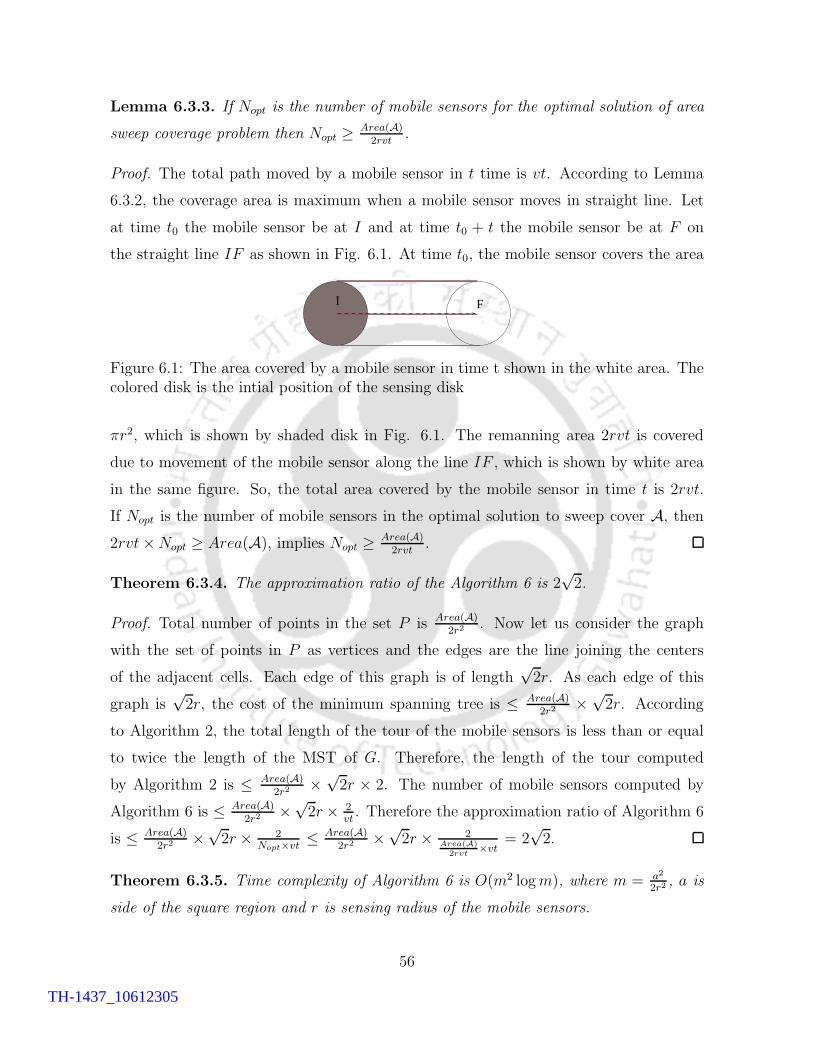
Lemma 6.3.3. If Nopt is the number of mobile sensors for the optimal solution of area
sweep coverage problem then Nopt ≥ Area(A)2rvt
.
Proof. The total path moved by a mobile sensor in t time is vt. According to Lemma
6.3.2, the coverage area is maximum when a mobile sensor moves in straight line. Let
at time t0 the mobile sensor be at I and at time t0 + t the mobile sensor be at F on
the straight line IF as shown in Fig. 6.1. At time t0, the mobile sensor covers the area
I F
Figure 6.1: The area covered by a mobile sensor in time t shown in the white area. Thecolored disk is the intial position of the sensing disk
πr2, which is shown by shaded disk in Fig. 6.1. The remanning area 2rvt is covered
due to movement of the mobile sensor along the line IF , which is shown by white area
in the same figure. So, the total area covered by the mobile sensor in time t is 2rvt.
If Nopt is the number of mobile sensors in the optimal solution to sweep cover A, then
2rvt×Nopt ≥ Area(A), implies Nopt ≥ Area(A)2rvt
.
Theorem 6.3.4. The approximation ratio of the Algorithm 6 is 2√2.
Proof. Total number of points in the set P is Area(A)2r2
. Now let us consider the graph
with the set of points in P as vertices and the edges are the line joining the centers
of the adjacent cells. Each edge of this graph is of length√2r. As each edge of this
graph is√2r, the cost of the minimum spanning tree is ≤ Area(A)
2r2×
√2r. According
to Algorithm 2, the total length of the tour of the mobile sensors is less than or equal
to twice the length of the MST of G. Therefore, the length of the tour computed
by Algorithm 2 is ≤ Area(A)2r2
×√2r × 2. The number of mobile sensors computed by
Algorithm 6 is ≤ Area(A)2r2
×√2r× 2
vt. Therefore the approximation ratio of Algorithm 6
is ≤ Area(A)2r2
×√2r × 2
Nopt×vt≤ Area(A)
2r2×√2r × 2
Area(A)2rvt
×vt= 2
√2.
Theorem 6.3.5. Time complexity of Algorithm 6 is O(m2 logm), where m = a2
2r2, a is
side of the square region and r is sensing radius of the mobile sensors.
56
TH-1437_10612305

Proof. We partition the square area a× a into√2r ×
√2r grid cells. So, total number
of grid cells is a2
2r2= m. Therefore, by Theorem 3.3.5, the time complexity of Algorithm
6 is O(m2 logm), where m = a2
2r2.
6.4 Improved Solution for Rectangular Region
In this section, we propose an improved solution of the problem for a rectangular region.
Let R be a rectangular region with sides a and b such that the sides are divisible by√2r. Divide R into square grids of side
√2r. Let m = a√
2rand n = b√
2r. Let P be the
set of center points of the grid cells. Let Gm,n be the grid graph corresponding to the
grid cells in P . Property of a grid graph Gm,n is given below as mentioned by Skiena
[56].
Property 1. Gm,n is Hamiltonian if either the number of rows or columns is even.
Figure 6.2: The movement path ofthe mobile sensors for m is even
Figure 6.3: The movement path ofthe mobile sensors for m = 4
Based on the above property, we consider following two cases to find a tour of Gm,n:
Case 1 Either m or n is even: Without loss of generality assume m is even. Accord-
ing to Property 1, a hamiltonian cycle can be found in this case. We draw the
hamiltonian cycle with length L (say), which is shown in Fig. 6.2. One particular
example is also shown in Fig. 6.3 for m = 4. In this case L =√2r ×mn.
Case 2 Both m and n are odd: We draw a cycle of length L (say), as shown in Fig.
6.4, which is a hamiltonian cycle for the corresponding complete graph G of Gm,n.
57
TH-1437_10612305

One particular example of the cycle is also shown in Fig. 6.5. Note that the
cycle contains only one edge which is not belongs to Gm,n. In this case L =√2r(mn− 1) + 2r.
Figure 6.4: The movement path ofthe mobile sensors for odd m and n
Figure 6.5: The movement path ofthe mobile sensors for m = 5 andn = 7
After finding the movement cycles in the both of the above cases, partition the cycles
into⌈
Lvt
⌉
parts and deploy⌈
Lvt
⌉
mobile sensors at all partitioning points, one for each.
Each mobile sensor starts moving at the same time along L in the same direction for
sweep coverage of R.
Theorem 6.4.1. The approximation factor of area sweep coverage algorithm for a grid
graph of even number of vertices is√2 and for odd number of vertices is
(√2 + 2−
√2
mn
)
.
Proof. Since length of the tour for case 1 is√2r×mn, the total number of mobile sensors
required for sweep coverage of R is dmn×√2r
vte. The approximation factor for this case is
mn×√2r
vt
/
2mnr2
2rvt=√2. Similarly, the approximation factor for case 2 is (mn−1)×
√2r+2r
vt
/
2mnr2
2rvt
=√2 + 2−
√2
mn.
6.5 Solution for Arbitrary Bounded Region
In this section, we consider area sweep coverage problem for an arbitrary bounded region.
Let A be an arbitrary bounded region. We divide the region A into square grids of side√2r. Since shape of the region is arbitrary, the grid cells, which are adjacent to the
perimeter P of the region may not be complete squares. The maximum number of
58
TH-1437_10612305
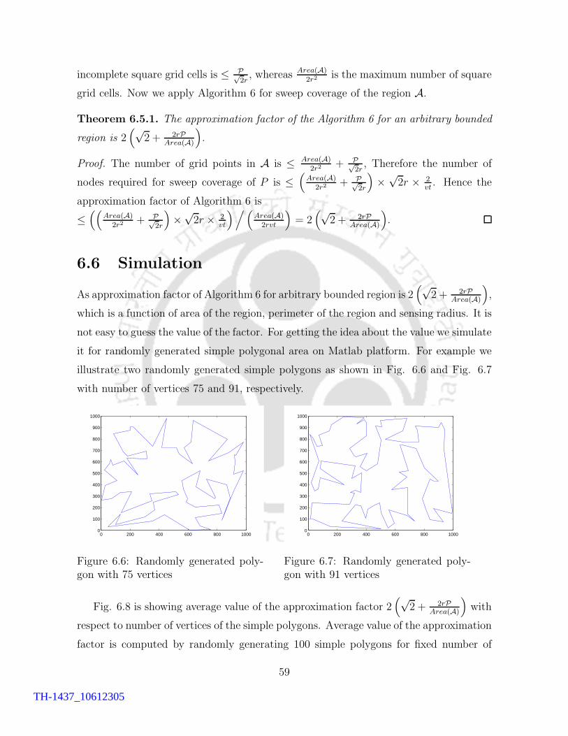
incomplete square grid cells is ≤ P√2r, whereas Area(A)
2r2is the maximum number of square
grid cells. Now we apply Algorithm 6 for sweep coverage of the region A.
Theorem 6.5.1. The approximation factor of the Algorithm 6 for an arbitrary bounded
region is 2(√
2 + 2rPArea(A)
)
.
Proof. The number of grid points in A is ≤ Area(A)2r2
+ P√2r, Therefore the number of
nodes required for sweep coverage of P is ≤(
Area(A)2r2
+ P√2r
)
×√2r × 2
vt. Hence the
approximation factor of Algorithm 6 is
≤((
Area(A)2r2
+ P√2r
)
×√2r × 2
vt
)/(
Area(A)2rvt
)
= 2(√
2 + 2rPArea(A)
)
.
6.6 Simulation
As approximation factor of Algorithm 6 for arbitrary bounded region is 2(√
2 + 2rPArea(A)
)
,
which is a function of area of the region, perimeter of the region and sensing radius. It is
not easy to guess the value of the factor. For getting the idea about the value we simulate
it for randomly generated simple polygonal area on Matlab platform. For example we
illustrate two randomly generated simple polygons as shown in Fig. 6.6 and Fig. 6.7
with number of vertices 75 and 91, respectively.
0 200 400 600 800 10000
100
200
300
400
500
600
700
800
900
1000
Figure 6.6: Randomly generated poly-gon with 75 vertices
0 200 400 600 800 10000
100
200
300
400
500
600
700
800
900
1000
Figure 6.7: Randomly generated poly-gon with 91 vertices
Fig. 6.8 is showing average value of the approximation factor 2(√
2 + 2rPArea(A)
)
with
respect to number of vertices of the simple polygons. Average value of the approximation
factor is computed by randomly generating 100 simple polygons for fixed number of
59
TH-1437_10612305
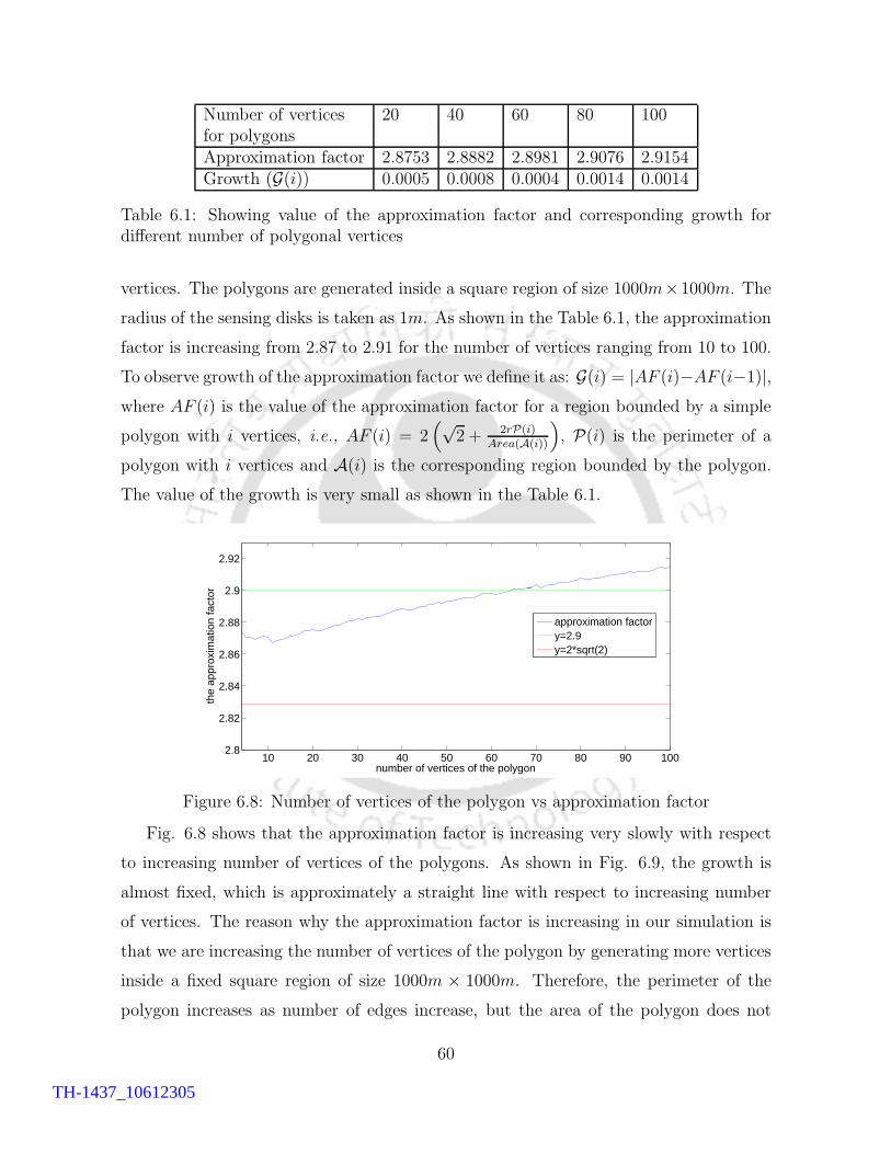
Number of vertices 20 40 60 80 100for polygonsApproximation factor 2.8753 2.8882 2.8981 2.9076 2.9154Growth (G(i)) 0.0005 0.0008 0.0004 0.0014 0.0014
Table 6.1: Showing value of the approximation factor and corresponding growth fordifferent number of polygonal vertices
vertices. The polygons are generated inside a square region of size 1000m×1000m. The
radius of the sensing disks is taken as 1m. As shown in the Table 6.1, the approximation
factor is increasing from 2.87 to 2.91 for the number of vertices ranging from 10 to 100.
To observe growth of the approximation factor we define it as: G(i) = |AF (i)−AF (i−1)|,where AF (i) is the value of the approximation factor for a region bounded by a simple
polygon with i vertices, i.e., AF (i) = 2(√
2 + 2rP(i)Area(A(i))
)
, P(i) is the perimeter of a
polygon with i vertices and A(i) is the corresponding region bounded by the polygon.
The value of the growth is very small as shown in the Table 6.1.
10 20 30 40 50 60 70 80 90 1002.8
2.82
2.84
2.86
2.88
2.9
2.92
number of vertices of the polygon
the
appr
oxim
atio
n fa
ctor
approximation factory=2.9y=2*sqrt(2)
Figure 6.8: Number of vertices of the polygon vs approximation factor
Fig. 6.8 shows that the approximation factor is increasing very slowly with respect
to increasing number of vertices of the polygons. As shown in Fig. 6.9, the growth is
almost fixed, which is approximately a straight line with respect to increasing number
of vertices. The reason why the approximation factor is increasing in our simulation is
that we are increasing the number of vertices of the polygon by generating more vertices
inside a fixed square region of size 1000m × 1000m. Therefore, the perimeter of the
polygon increases as number of edges increase, but the area of the polygon does not
60
TH-1437_10612305
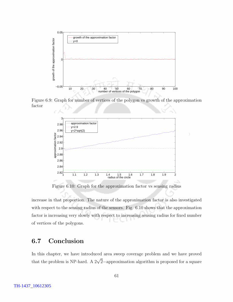
10 20 30 40 50 60 70 80 90 100−0.05
0
0.05
number of vertices of the polygon
grow
th o
f the
app
roxi
mat
ion
fact
or
growth of the approximation factory=0
Figure 6.9: Graph for number of vertices of the polygon vs growth of the approximationfactor
1 1.1 1.2 1.3 1.4 1.5 1.6 1.7 1.8 1.9 22.82
2.84
2.86
2.88
2.9
2.92
2.94
2.96
2.98
3
radius of the circle
appr
oxim
atio
n fa
ctor
approximation factory=2.9y=2*sqrt(2)
Figure 6.10: Graph for the approximation factor vs sensing radius
increase in that proportion. The nature of the approximation factor is also investigated
with respect to the sensing radius of the sensors. Fig. 6.10 shows that the approximation
factor is increasing very slowly with respect to increasing sensing radius for fixed number
of vertices of the polygons.
6.7 Conclusion
In this chapter, we have introduced area sweep coverage problem and we have proved
that the problem is NP-hard. A 2√2−approximation algorithm is proposed for a square
61
TH-1437_10612305

region. The approximation factor is improved for rectangular region. We have solved
sweep coverage for arbitrary bounded regions, where the approximation factor of the so-
lution is a function of perimeter, area of the region and sensing radius. With simulation,
we have investigated how the approximation factor varies for arbitrary region, bounded
by simple polygon.
62
TH-1437_10612305

Chapter 7
Barrier Sweep Coverage
7.1 Introduction
Periodic monitoring is important to protect our national borders from unauthorized
immigration, terrorist activities, illegal movement of weapons, drugs, etc. It is also im-
portant to detect spread of pollutants, chemicals, etc, in an industrial township. In most
of the previous works on barrier coverage [12, 36, 42, 49, 65], static sensors are deployed
for continuous monitoring of the borders or boundaries. But for the aforementioned
types of applications, deployment of static sensors at the borders are not cost effective
in terms of resource utilization. Coverage requirement for those applications is time-
variant. An efficient solution can be provided by utilizing less number of mobile sensors
with appropriate movement strategy. The cost involvement aspect of this solution is mo-
bility and storage capacity of the mobile sensors. In this chapter we study barrier sweep
coverage with mobile sensors where a barrier is considered as a finite length continuous
curve in a plane. The coverage at every point on a curve is time-variant. Throughout
this chapter, by finite curve we mean a continuous curve of finite length.
7.1.1 Contribution
Our contributions in this chapter are as follows:
• We introduce barrier sweep coverage concept for covering finite curves in a plane.
The problem is solved optimally with minimum number of mobile sensors.
63
TH-1437_10612305

• An energy restricted barrier sweep coverage problem is defined and a 133-approximation
algorithm is proposed to solve it for a finite curve.
• Barrier sweep coverage problem for multiple finite curves (BSCMC) is also pro-
posed and proved that the problem is NP-hard and cannot be approximated within
a factor of 2, unless P=NP. A 2-approximation algorithm is proposed to solve the
problem for a special case. A 5-approximation algorithm is proposed to solve
BSCMC.
• We formulate a data gathering problem, where a set of data mules is used for gath-
ering data and prove that the problem is NP-hard. A 3-approximation algorithm
is proposed to solve it.
• Through simulation, we investigate performance of the proposed algorithms for
multiple finite curves.
7.2 Problem Definitions
Let C be a finite curve on a two dimensional plane. C is said to be covered by a set of
sensors if and only if each point on C is covered by at least one sensor. Based on this
coverage metric, we give the definitions of barrier sweep coverage as follows.
Definition 7.2.1. (t-barrier sweep coverage) Let C be any finite curve on a two
dimensional plane and M={m1,m2,· · · , mp} be a set of mobile sensors. C is said to be
t-barrier sweep covered if and only if each point of C is visited by at least one mobile
sensor in every time period t.
Problem 8. (Barrier sweep coverage problem for single finite curve) Let C be
a finite curve and M={m1,m2,· · · , mp} be a set of mobile sensors. Let v be the uniform
speed of the mobile sensors. For a given t > 0, find the minimum number of mobile
sensors such that C is t-barrier sweep covered.
Problem 9. (Barrier sweep coverage problem for multiple finite curves (BSCMC))
Let X = {C1, C2, · · · , Cn} be a set of finite curves and M={m1,m2,· · · , mp} be a set of
64
TH-1437_10612305

mobile sensors. Let v be the uniform speed of the mobile sensors. For a given t > 0, find
the minimum number of mobile sensors such that each Ci for i = 1, 2, · · · , n is t-barrier
sweep covered.
In general sensors are equipped with limited battery power. In order to continue
sweep coverage for long time, each mobile sensor must visits an energy source to recharge
or replace its battery. Let Γ be the maximum travel time for a mobile sensor starting
with full powered battery maintaining uniform speed v till battery power goes off. Let
e be an energy source in the plane and every mobile sensor can recharge or replace its
battery by visiting e. We define energy restricted barrier sweep coverage problem for a
finite curve C as given below.
Problem 10. (Energy restricted barrier sweep coverage problem) Let C be a
finite curve and M={m1,m2,· · · , mp} be a set of mobile sensors. Let v be the uniform
speed of the mobile sensors. Let e be an energy source in the plane. For given t,Γ > 0,
find the minimum number of mobile sensors such that C is t-barrier sweep covered and
each mobile sensor visits e once in every Γ time period.
7.3 Barrier Sweep Coverage for a finite Curve
In this section, first we propose a solution for finding the optimal number of mobile
sensors to sweep cover a finite curve. Later, we give an approximate solution for the
energy restricted barrier sweep coverage problem for a finite curve.
7.3.1 Optimal solution for a finite curve
The barrier sweep coverage problem for a finite curve can be optimally solved using the
following strategy. Let |C| be the length of the finite curve C. If C is a closed curve,
then partition C into⌈
|C|vt
⌉
equal parts of length vt and deploy⌈
|C|vt
⌉
mobile sensors at
the partitioning points, one for each. Then all mobile sensors start moving at same time
along C in the same direction to ensure t-barrier sweep coverage of C. If C is an open
curve, then join the end points of C to make it close and apply the strategy for closed
curve.
65
TH-1437_10612305
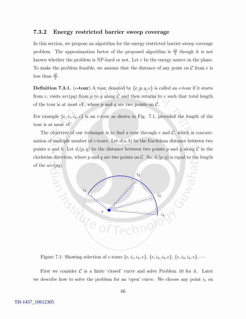
7.3.2 Energy restricted barrier sweep coverage
In this section, we propose an algorithm for the energy restricted barrier sweep coverage
problem. The approximation factor of the proposed algorithm is 133
though it is not
known whether the problem is NP-hard or not. Let e be the energy source in the plane.
To make the problem feasible, we assume that the distance of any point on C from e is
less than vΓ2.
Definition 7.3.1. (e-tour) A tour, denoted by {e, p, q, e} is called an e-tour if it starts
from e, visits arc(pq) from p to q along C and then returns to e such that total length
of the tour is at most vΓ, where p and q are two points on C.
For example {e, i1, i2, e} is an e-tour as shown in Fig. 7.1, provided the length of the
tour is at most vΓ.
The objective of our technique is to find a tour through e and C, which is concate-
nation of multiple number of e-tours. Let d(a, b) be the Euclidean distance between two
points a and b. Let dc(p, q) be the distance between two points p and q along C in the
clockwise direction, where p and q are two points on C. So, dc(p, q) is equal to the length
of the arc(pq).
i1
i2
i3
i4e
Figure 7.1: Showing selection of e-tours {e, i1, i2, e}, {e, i2, i3, e}, {e, i3, i4, e}, · · ·
First we consider C is a finite ‘closed’ curve and solve Problem 10 for it. Later
we describe how to solve the problem for an ‘open’ curve. We choose any point i1 on
66
TH-1437_10612305

C. Find a point i2 on C in the clockwise direction from i1 (Ref. Fig. 7.1) such that
Algorithm 7 EnergyRestrictedBSC
1: Choose any point i1 on C.2: C′ = C, n′ = 1.3: while C′ 6= φ do4: if d(e, in′) + |C′| ≤ vΓ
2then
5: h = i1.6: else7: Select a point h on C in a clockwise direction from in′ such that d(in′, h) =
vΓ2− d(e, in′).
8: end if9: if n′ 6= 1 and d(e, in′−1) + dc(in′−1, h) + d(e, h) ≤ vΓ then10: C′ = C′ \ arc(in′h).11: in′ = h, Tn′−1 = {e, in′−1, in′, e}.12: else13: in′+1 = h, Tn′ = {e, in′ , in′+1, e}.14: C′ = C′ \ arc(in′in′+1).15: n′ = n′ + 1.16: end if17: C′ = C′ \ arc(in′in′+1).18: end while19: APPRX = T1 · T2 · T2 · · · · · Tn′ , where ‘·’ is denoted as concatenation operation.20: Divide APPRX into equal parts of length vt and deploy one mobile sensor at each
of the partitioning points.21: All mobile sensor start moving along APPRX at same time in same direction.
dc(i1, i2) =vΓ2− d(e, i1). Here T1 = {e, i1, i2, e} is an e-tour, since length of T1 is equal
to d(e, i1) + dc(i1, i2) + d(i2, e) ≤ d(e, i1) +vΓ2− d(e, i1) +
vΓ2
= vΓ, as shown in the Fig.
7.1. Next e-tour is selected as {e, i2, i3, e}, where i3 is a point on C in the clockwise
direction from i2 such that dc(i2, i3) =vΓ2− d(e, i2). Once the second tour is selected,
we check whether the combination of the previous tour and current tour together, i.e.,
{e, i1, i3, e} forms an e-tour or not. If the combined tour {e, i1, i3, e} is a valid e-tour,
then the previous tour {e, i1, i2, e} is updated into {e, i1, i3, e} and we proceed to select
the next e-tour. This updating process continues until combined tour violates the length
constraint of e-tour. In general, after computing an e-tour Tj = {e, ij, ij+1, e}, we select
next point ij+2 on C such that dc(ij+1, ij+2) =vΓ2− d(e, ij+1). Then if {e, ij, ij+2, e} this
is a valid e-tour, we update the tour Tj as Tj = {e, ij , ij+2, e}. Otherwise the tour Tj+1
67
TH-1437_10612305
is selected as Tj+1 = {e, ij+1, ij+2, e}. Finally C is decomposed into multiple number of
e-tours such that every point on C is included in some e-tour.
If C is an ‘open’ curve, we use the above technique to decompose C into multiple
number of e-tours considering one end point of C as i1 and continue till the other end
point. Note that according to the construction of the e-tours, length of the combined
tour of any two consecutive e-tours is always greater than vΓ.
Let APPRX be the total tour after concatenation of the e-tours, T1, T2, T3, · · · one
after another in order of obtained by the above technique. For example T1 = {e, i1, i2, e},T2 = {e, i2, i3, e}, T3 = {e, i3, i4, e}, · · · are e-tours as shown in the Fig. 7.1, where
concatenation of those tours is T1 · T2 · T3 · · · · ={e, i1, i2, e} · {e, i2, i3, e} · {e, i3, i4, e} · · · ·= {e, i1, i2, e, i2, i3, e, i3, i4, e, · · · }, where ‘·’ is denoted as the concatenation operation of
the e-tours. Let |APPRX| be the length of APPRX . Divide APPRX into equal parts
of length vt and deploy one mobile sensor at each of the partitioning points. The mobile
sensors then start moving along APPRX in the same direction to ensure sweep coverage
of C. The Algorithm 7 (EnergyRestrictedBSC) for energy restricted barrier sweep
coverage is proposed for a closed curve. But as explained above it is also applicable for
an open curve.
Theorem 7.3.2. According to Algorithm 7, each mobile sensor visits e in every Γ time
period and each point on C is visited by at least one mobile sensor in every t time period.
Proof. Mobile sensors move along the tour APPRX according to movement strategy of
Algorithm 7. As length of each e-tour is less than or equals to vΓ, the mobile sensors
visit e after traveling at most vΓ distance since its last visit of e. Therefore, each mobile
sensor visits e once in every Γ time period. Again, the mobile sensors are deployed at
every partitioning points of APPRX and two consecutive partitioning points are within
vt distance apart. The relative distance between any two consecutive mobile sensors is
at most vt at any time as they are moving in same speed v and same direction. So,
when any point p on C is visited by a mobile sensor at t0, another mobile sensor was on
the way to p and within the distance of vt along APPRX . Hence p will be again visited
by another mobile sensor within next t time.
To analyze the approximation factor of Algorithm 7, we consider some special points
68
TH-1437_10612305

on C. Let i1p, i2p be two special points on the arc(ipip+1) of C such that the arc(ipip+1)
is partitioned into three equal parts, i.e., the length of arc(ipi1p) equal to the length of
arc(i1pi2p) equal to the length of arc(i2pip+1). We define a set of points, I = {ij , i1j , i2j |j =
1 to n′}. Following two lemmas give an upper bound of the length of the tour APPRX
and a lower bound of the length of the optimal tour respectively.
Lemma 7.3.3. |APPRX| ≤ 1
3
(
2∑
j
(
d(e, ij) + d(e, i1j ) + d(e, i2j))
+ 5|C|)
.
Proof. According to Algorithm 7, total length of the tour APPRX is
|APPRX| = d(e, i1) + dc(i1, i2) + d(i2, e) + d(e, i2) + dc(i2, i3)
+d(i3, e) + · · ·+ d(e, i1)
= |C|+ 2∑
j
d(e, ij). (7.3.1)
Now by triangle inequality,
d(e, ij) ≤ d(e, i1j) + dc(ij , i1j ) and
d(e, ij) ≤ d(e, i2j) + dc(ij , i2j ).
Therefore,
|APPRX| ≤ |C|+ 2∑
j
(
d(e, i1j ) + dc(ij , i1j))
. (7.3.2)
|APPRX| ≤ |C|+ 2∑
j
(
d(e, i2j ) + dc(ij , i2j))
. (7.3.3)
From the above Equation 7.3.1, 7.3.2 and 7.3.3, we can write,
3|APPRX| ≤ 3|C|+ 2∑
j
d(e, ij) + 2∑
j
(
d(e, i1j ) + dc(ij , i1j))
+2∑
j
(
d(e, i2j ) + dc(ij , i2j))
. (7.3.4)
69
TH-1437_10612305

As the points i1j and i2j divide length of the arc(ijij+1) into three equal parts, therefore,∑
j
dc(ij , i1j) =
|C|3
and∑
j
dc(ij , i2j) =
2|C|3
.
Using these two results, Equation 7.3.4 can be written as:
3|APPRX| ≤ 3|C|+ 2∑
j
(
d(e, ij) + d(e, i1j) + d(e, i2j ))
+ 2|C|3
+4|C|3
|APPRX| ≤ 1
3
(
2∑
j
(
d(e, ij) + d(e, i1j) + d(e, i2j))
+ 5|C|)
.
p
ijij+1
ij−1
q
ij+2e
Figure 7.2: Showing one e-tour OPTl = {e, p, q, e} of the optimal tour OPT
Lemma 7.3.4. Let OPT be the optimal tour of the mobile sensors and |OPT | be length
of OPT , then |OPT | ≥ max
{
1
4
∑
j
(
d(e, ij) + d(e, i1j ) + d(e, i2j))
, |C|}
.
Proof. Let OPTl = {e, p, q, e} be an e-tour of the optimal tour OPT (Ref. Fig. 7.2).
We claim that at most one arc(ijij+1), part of an e-tour computed using Algorithm 7
for some j, can be completely contained in arc(pq), where arc(pq) is a part of OPTl.
To prove this, let us assume that there are two such arcs arc(ij−1ij) and arc(ijij+1)
completely contained in arc(p, q). As length of combined tour of two consecutive e-tours
is always greater than vΓ according to step 12 of Algorithm 7, therefore,
(d(e, ij−1) + dc(ij−1, ij+1) + d(e, ij+1)) > vΓ. (7.3.5)
70
TH-1437_10612305
Now,
|OPTl| = d(e, p) + dc(p, ij−1) + dc(ij−1, ij) + dc(ij , ij+1) + dc(ij+1, q) + d(e, q)
≥ d(e, ij−1) + dc(ij−1, ij+1) + d(e, ij+1)
> vΓ (from Equation 7.3.5).
This contradicts the fact that OPTl is an e-tour. Therefore, at most one arc(ijij+1) for
some j, can be completely contained in arc(pq). Hence, at most one complete arc(ijij+1)
and two arc(ij−1ij) and arc(ij+1ij+2) partially contained in arc(pq) as shown in Fig. 7.2.
Therefore, maximum eight points from the set I may belong to the arc(pq), since there
are four points ij , i1j , i
2j , ij+1 for the arc(ijij+1) and at most four special points, i1j−1,
i2j−1 and i1j+1, i2j+1 for the arc(ij−1ij) and arc(ij+1ij+2) respectively.
Now, for any point x on arc(pq) of OPTl implies |OPTl| ≥ 2d(e, x). As there are at
most eight points of I in arc(pq), which implies
|OPTl| ≥2∑
x ∈ I∩arc(pq) d(e, x)
8. (7.3.6)
Since all the points in I are on arc(pq) for some OPTl, where OPTl is a part of OPT ,
therefore,
|OPT | ≥∑
l
|OPTl| ≥2∑
j
(
d(e, ij) + d(e, i1j) + d(e, i2j))
8. Also, |OPT | ≥ |C|.
Hence, |OPT | ≥ max
{
1
4
∑
j
(
d(e, ij) + d(e, i1j) + d(e, i2j))
, |C|}
.
Theorem 7.3.5. The approximation factor of Algorithm 7 is13
3.
Proof. Let N be the number of mobile sensors needed in our solution and Nopt be the
number of mobile sensors in the optimal solution.
Then N =
⌈ |APPRX|vt
⌉
and Nopt ≥|OPT |vt
. From Lemma 7.3.3 and Lemma 7.3.4, we
haveN
Nopt
≤ |APPRX||OPT | ≤ 8
3+
5
3=
13
3. Hence the approximation factor of our proposed
Algorithm 7 is13
3.
71
TH-1437_10612305
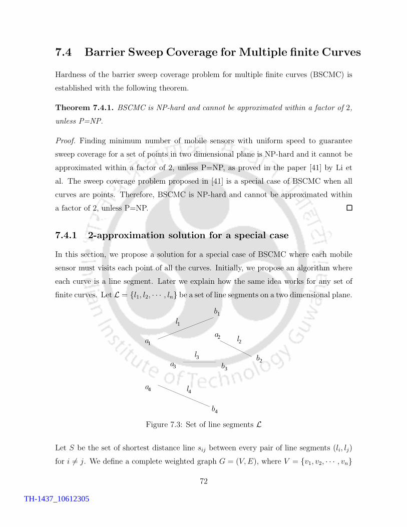
7.4 Barrier Sweep Coverage for Multiple finite Curves
Hardness of the barrier sweep coverage problem for multiple finite curves (BSCMC) is
established with the following theorem.
Theorem 7.4.1. BSCMC is NP-hard and cannot be approximated within a factor of 2,
unless P=NP.
Proof. Finding minimum number of mobile sensors with uniform speed to guarantee
sweep coverage for a set of points in two dimensional plane is NP-hard and it cannot be
approximated within a factor of 2, unless P=NP, as proved in the paper [41] by Li et
al. The sweep coverage problem proposed in [41] is a special case of BSCMC when all
curves are points. Therefore, BSCMC is NP-hard and cannot be approximated within
a factor of 2, unless P=NP.
7.4.1 2-approximation solution for a special case
In this section, we propose a solution for a special case of BSCMC where each mobile
sensor must visits each point of all the curves. Initially, we propose an algorithm where
each curve is a line segment. Later we explain how the same idea works for any set of
finite curves. Let L = {l1, l2, · · · , ln} be a set of line segments on a two dimensional plane.
4
1
1
1
2
2
2
3 3
3
4
4
a
a
aa
b
bb
b
l
l
l
l
Figure 7.3: Set of line segments L
Let S be the set of shortest distance line sij between every pair of line segments (li, lj)
for i 6= j. We define a complete weighted graph G = (V,E), where V = {v1, v2, · · · , vn}
72
TH-1437_10612305
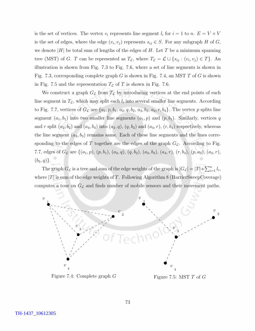
is the set of vertices. The vertex vi represents line segment li for i = 1 to n. E = V ×V
is the set of edges, where the edge (vi, vj) represents sij ∈ S. For any subgraph H of G,
we denote |H| be total sum of lengths of the edges of H . Let T be a minimum spanning
tree (MST) of G. T can be represented as TL, where TL = L ∪ {sij : (vi, vj) ∈ T}. An
illustration is shown from Fig. 7.3 to Fig. 7.6, where a set of line segments is shown in
Fig. 7.3, corresponding complete graph G is shown in Fig. 7.4, an MST T of G is shown
in Fig. 7.5 and the representation TL of T is shown in Fig. 7.6.
We construct a graph GL from TL by introducing vertices at the end points of each
line segment in TL, which may split each li into several smaller line segments. According
to Fig. 7.7, vertices of GL are {a1, p, b1, a2, q, b2, a3, b3, a4, r, b4}. The vertex p splits line
segment (a1, b1) into two smaller line segments (a1, p) and (p, b1). Similarly, vertices q
and r split (a2, b2) and (a4, b4) into (a2, q), (q, b2) and (a4, r), (r, b4) respectively, whereas
the line segment (a3, b3) remains same. Each of these line segments and the lines corre-
sponding to the edges of T together are the edges of the graph GL. According to Fig.
7.7, edges of GL are {(a1, p), (p, b1), (a2, q), (q, b2), (a3, b3), (a4, r), (r, b4), (p, a3), (a3, r),(b3, q)}.
The graphGL is a tree and sum of the edge weights of the graph is |GL|= |T |+∑n
i=1 li,
where |T | is sum of the edge weights of T . Following Algorithm 8 (BarrierSweepCoverage)
computes a tour on GL and finds number of mobile sensors and their movement paths.
v
v
v
v1
2
3
4
Figure 7.4: Complete graph G
v
v
v
v1
2
3
4
Figure 7.5: MST T of G
73
TH-1437_10612305
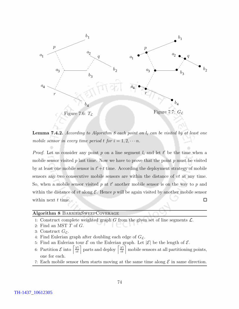
4
1
1
2
23
3
4a
a
aa
b
b
b
b
p
q
r
Figure 7.6: TL
4
1
1
2
233
4a
a
aa
b
bb
b
p
q
r
Figure 7.7: GL
Lemma 7.4.2. According to Algorithm 8 each point on li can be visited by at least one
mobile sensor in every time period t for i = 1, 2, · · ·n.
Proof. Let us consider any point p on a line segment li and let t′ be the time when a
mobile sensor visited p last time. Now we have to prove that the point p must be visited
by at least one mobile sensor in t′+ t time. According the deployment strategy of mobile
sensors any two consecutive mobile sensors are within the distance of vt at any time.
So, when a mobile sensor visited p at t′ another mobile sensor is on the way to p and
within the distance of vt along E . Hence p will be again visited by another mobile sensor
within next t time.
Algorithm 8 BarrierSweepCoverage
1: Construct complete weighted graph G from the given set of line segments L.2: Find an MST T of G.3: Construct GL.4: Find Eulerian graph after doubling each edge of GL.5: Find an Eulerian tour E on the Eulerian graph. Let |E| be the length of E .6: Partition E into
⌈
|E|vt
⌉
parts and deploy⌈
|E|vt
⌉
mobile sensors at all partitioning points,
one for each.7: Each mobile sensor then starts moving at the same time along E in same direction.
74
TH-1437_10612305
Lemma 7.4.3. If Lopt is the length of the optimal TSP tour for visiting all points of
every line segment in L, then |T |+∑n
i=1 li ≤ Lopt.
Proof. The optimal TSP tour Lopt contains two types of movement paths; movement
paths along the line segments of L and movement paths between the line segments. Let
total length of the movement paths along the line segments be Lalong. Since Lopt is the
optimal tour for visiting all points of each line segment li ∈ L, therefore,
Lalong ≥n∑
i=1
li. (7.4.1)
Let LG be the optimal TSP tour on G. Then |T | ≤ LG. Let total length of the movement
paths between the line segments be Lbetween. Since LG is the optimal TSP tour on G and
the weights of all edges of G are taken to be the shortest distance between respective
line segments, therefore,
Lbetween ≥ LG. (7.4.2)
Now, from Equation 7.4.1 and 7.4.2, LG+∑n
i=1 li ≤ Lopt. Hence |T |+∑n
i=1 li ≤ Lopt.
Theorem 7.4.4. The approximation factor of Algorithm 8 is 2.
Proof. The total edge weights of GL is |T |+∑ni=1 li. Now, |E| = 2(|T |+∑n
i=1 li), since
Eulerian tour E found by Algorithm 8 after doubling each edges of GL. By Lemma 7.4.3,
|E| ≤ 2Lopt. Let Nopt be the number of mobile sensors required for optimal solution.
Then Nopt × vt ≥ Lopt, i.e., Nopt ≥⌈
Lopt
vt
⌉
. The number of mobile sensors calculated by
Algorithm 8 is⌈
|E|vt
⌉
(=N , say). Therefore, the approximation factor of Algorithm 8 is
equal to NNopt
≤⌈
2Lopt
vt
⌉/⌈
Lopt
vt
⌉
≤ 2.
7.4.2 Solution for BSCMC
In this section, we propose an algorithm for the BSCMC problem, where each curve is
a line segment. The description of the algorithm is given below.
For k = 1 to n following calculations are performed. Compute a minimum spanning
forest Fk of G with k components. Let C1, C2, · · · , Ck be the connected components
of Fk. Let C iL be a representation of C i on the set of line segments L for i = 1 to
75
TH-1437_10612305
k, where C iL = {lj |vj ∈ C i} ∪ {sij |(vi, vj) ∈ C i}. Construct graph Gi
L from C iL in the
same way GL is constructed from TL in Section 7.4.1. Clearly,∑k
i=1 |GiL| =
∑nj=1 lj +
|Fk|. Find Eulerian tours E1L, E2
L, · · · , EkL after doubling the edges of G1
L, G2L, · · · ,
GkL respectively. Partition each Ek
L into⌈
|EkL|
vt
⌉
parts of length vt. Let Nk be the total
number of partitioning points. Choose the minimum over all Nk’s as the number of
mobile sensors. Deploy the number of mobile sensors, one at each of the partitioning
points. Then all mobile sensors start their movement at the same time along their
respective tours in the same direction.
Theorem 7.4.5. The approximation factor of the proposed solution for BSCMC is 5.
Proof. Let opt be the number of mobile sensor required for the optimal solution of
BSCMC. Let opt′ be the minimum number of mobile sensor which can guarantee t-
sweep coverage of all the vertices of G. Then opt ≥ opt′.
Since, all the points of each line segments are visited by the mobile sensors in any
time period t then opt ≥∑n
i=1 livt
. Let us consider the movement paths of opt′ number
of mobile sensors to sweep cover the vertices of G in any time interval [t0, t + t0]. Let
Min path be total sum of lengths of the paths. Then Min path ≤ vt×opt′. Again these
opt′ movement paths form a spanning forest with opt′ number of connected components
of G. Therefore, we have |Fopt′| ≤ Min path as Fopt′ is the minimum spanning forest of
G with opt′ components. Let us consider the iteration of our solution for k = opt′. Total
number of mobile sensors N in this iteration is given below.
N =∑k
i=1
⌈
|EiL|
vt
⌉
≤ ∑ki=1
|EiL|
vt+ k = 2
∑ki=1
|GiL|
vt+ k = 2
∑ni=1 livt
+ 2 |Fk|vt
+ k ≤ 2opt +
2Min path
vt+ k ≤ 2opt+ 2opt′ + opt′ ≤ 5opt.
Therefore, the approximation factor of our proposed solution is 5.
The two algorithms proposed in this section also work for a set of finite curves as
explained below. Let X be a set of finite curves and S be the set of shortest distance line
between every pair of the curves. The complete weighted graph G can be constructed
considering each curve as a vertex and the distance between every pair of curves as an
edge weight corresponding to the edge. For the MST or any subtree of G, Eulerian tour
on the tree or the subtree can be form in the same way by introducing vertices at the
end points of each curve and doubling the edges. Mobile sensors also can be deployed
76
TH-1437_10612305

after partitioning the tours at each of the partitioning points. The mobile sensors follow
same movement strategy as earlier to guarantee sweep coverage of the multiple finite
curves.
7.5 Data Gathering by Data Mules
In this section, we consider a data gathering problem by a set of data mules [2, 10, 37, 38,
53], which we formulate as a variation of barrier sweep coverage problem. A set of mobile
sensors are moving along finite straight lines in a plane for monitoring or sampling data.
Movement of the mobile sensors are arbitrary along their respective paths i.e., a mobile
sensor moves in any direction along the straight line with arbitrary speed. A set of data
mules are moving with uniform speed v in the same plane for collecting data from the
mobile sensors. A data mule can collect data from a mobile sensor whenever it meets
the mobile sensor on its path. We assume data transfer can be done instantaneously
whenever a data mule meets a mobile sensor. In the data gathering applications, a data
mule collects data from all the mobile sensors one by one visiting them and relay the
collected data to the sink. The definition of the problem is given below.
Problem 11 (Minimum number of data mule for data gathering (MDMDG)). A set
of mobile sensors are moving arbitrarily in a plane along line segments. Find minimum
number of data mules with uniform speed v such that
1. each mobile sensor is visited by a data mule at least once in every t time period for
collecting data,
2. each data mule visits all mobile sensors.
The sweep coverage problem [41] is a special instance of MDMDG when two end
points of every line segment are same, i.e. the mobile sensors are behaving like a static
sensor. Therefore we can state the following theorem.
Theorem 7.5.1. MDMDG is NP-hard and cannot be approximated within a factor of
2, unless P=NP.
77
TH-1437_10612305

The proof of the above theorem directly follows from Theorem 7.4.1. Following
Lemma 7.5.2 shows that to visit the mobile sensors, each point of all paths must be
visited by the data mules.
Lemma 7.5.2. To solve MDMDG each and every point of all line segments must be
visited by the set of data mules.
Proof. We prove the lemma by the method of contradiction. Let l be a line segment
for which all points of l are not visited by the data mules. Therefore, there exist one
point p on l such that p is not visited by any data mule. One mobile sensor can stop
its movement for sometime and which can be allowed for the arbitrary nature of its
movements. Now, if the mobile sensor on l remains static at p for more than t time
then it will not be visited by any data mule in a time period t, which is a contradiction.
Hence, each and every point of all line segments must be visited by the set of data
mules.
Now, we find the minimum path traveled by a single data mule to visit all the
mobile sensors. According to the problem definition and by Lemma 7.5.2, within any
time interval [t0, t0 + t], all points of each line segment are visited by the data mules.
Therefore, total length of the tour traversed by all the data mules within the time interval
is greater or equals to the optimal tour traversed by a single data mule. Following lemma
gives the nature of the optimal tour traversed by a single data mule for visiting all the
mobile sensors.
Lemma 7.5.3. It may not be possible to visit a mobile sensor by a data mule unless the
data mule visits the whole line segment from one end to the other end continuously.
Proof. If a line segment is not visited ‘continuously’ then in the following scenario the
data mule cannot visit a mobile sensor. Let l′ and l′′ be the two parts of a line segment
l. There is a time gap between two continuous visits of l′ and l′′ by the data mule. It
may happen that during the visit of l′ the mobile sensor remains on l′′ and during the
visit of l′′ the mobile sensor remains on l′. The mobile sensor changes its position during
the time gap. So, in this scenario the data mule cannot visit mobile sensor.
78
TH-1437_10612305
Let Lopt be the optimal tour for visiting all mobile sensors by one data mule. Now,
the optimal tour Lopt contains two types of movement paths: the movement paths along
the line segments and the paths between pair of line segments. According to Lemma
7.5.3, the paths between pair of line segments are the lines which connect end points of
the pair of line segments. We construct Euclidian complete graph G2n with 2n vertices
ai, bi, i = 1, 2, · · ·n, where ai and bi are two end points of the line li. The edge set E(G2n)
of G2n is given by E(G2n) = {li : i = 1, 2, · · · , n} ∪ {(ai, aj) : i 6= j} ∪ {(bi, bj) : i 6=j}∪{(ai, bj) : i 6= j}∪{(bi, aj) : i 6= j}. The weight of each edge is equal to the Euclidian
distance between two vertices of the edge. Let T2n be a MST of G2n containing all edges
li ∈ E(T2n), i = 1, 2, · · · , n. We compute T2n using Kruskal’s algorithm after including
all edges li, i = 1, 2, · · · , n in the initial edge set of T2n. Until the spanning tree is formed,
we apply Kruskal’s algorithm on the remaining edges, E(G2n)\{li : i = 1, 2, · · · , n} of
G2n. An Eulerian graph is formed from T2n as described in Christofides algorithm [13].
We compute an Eulerian tour E2n from the above Eulerian graph.
We cannot directly apply the movement strategy of the mobile sensors, which is used
in Algorithm 7 and Algorithm 8 to give the movement strategy of the data mules. If
there exist a line segment with length greater than vt and the mobile sensor moves with
a speed v along the line in the same direction as the data mule moves then it may not
be possible by the data mule to meet the mobile sensor within time t. Hence, we apply
a new strategy as explained below in order solve the MDMDG problem.
Partition the tour E2n into equal parts of length vt and consider two sets of data
mules DM1 and DM2, each of which contains dE2nvte number of data mules. Deploy two
data mules at each of the partitioning points one from each set. Then each data mule
from the set DM1 moves in a clockwise direction, whereas other set of data mules DM2
move in the counter clockwise direction. All data mules, irrespective of the sets start
their movement at same time. Based on the above discussions, we propose following
Algorithm 9 (MDMDG).
79
TH-1437_10612305
Algorithm 9 MDMDG
1: Use Kruskal algorithm to find an MST T2n of G2n with the initial set of edgescontaining all edges li for i = 1, 2, · · · , n.
2: Construct an Eulerian graph from T2n using Christofides algorithm [13].3: Find an Eulerian tour E2n from the Eulerian graph. Let |E2n| be the length of E2n.4: Partition E2n into
⌈
|E2n|vt
⌉
parts of length vt. Deploy two data mules, one from DM1
and other from DM2 at each of the partitioning points.5: All data mules start moving at the same time along E2n such that the data mules
from DM1 move in clockwise direction and the data mules from DM2 move inanticlockwise direction.
7.5.1 Analysis
Theorem 7.5.4. Each mobile sensor is visited by a data mule at least once in every t
time period according to Algorithm 9.
Proof. Let position of a mobile sensor be p when it visited last time by a data mule at
time t0. According the deployment strategy of data mules, two data mules visit p again
within time t0 + t, from two different directions. The statement of the theorem follows
if the mobile sensor remains static at p till t0 + t. Now we consider the case when the
mobile sensor moves clockwise direction from p after time t0. In this case there exist a
data mule, which is moving in counter clockwise direction that visits the mobile sensor
within time t0+ t. Similarly, if the mobile sensor moves counter clockwise direction from
p after time t0, then there exist a data mule, which is moving in clockwise direction that
visits the mobile sensor within time t0+t. Hence, irrespective of the nature of movement,
a mobile sensor is visited by a data mule at least once in every t time period.
Theorem 7.5.5. The approximation factor of Algorithm 9 is 3.
Proof. According to the Christofides algorithm [13] we can write |E2n| ≤ 32Lopt. Let Nopt
be the number of data mules required for optimal solution.
Then Nopt × vt ≥ Lopt, i.e., Nopt ≥⌈
Lopt
vt
⌉
. The number of data mule (N) calculated
by the Algorithm 9 is⌈
2|E2n|vt
⌉
. Therefore, the approximation factor for Algorithm 9 is
equal to NNopt
≤⌈
2× 32Lopt
vt
⌉/⌈
Lopt
vt
⌉
≤ 3.
80
TH-1437_10612305

7.6 Simulation Results
To the best of our knowledge there is no related work on barrier sweep coverage problem
in literature. We compare performance of our proposed Algorithm 8 and the algorithm
for BSCMC through simulation. We implement both of the algorithms in C++ language.
A set of line segments are randomly generated inside a square region of side 200 meter.
The length of each line segment is randomly chosen within 5 meter. The uniform speed
of each mobile sensor is taken as 1 meter per second.
No. of line segments Number of Mobile SensorsAlgorithm for BSCMC Algorithm 8
5 5 1215 14 2825 21 3535 26 4345 35 5455 42 6465 51 7275 57 7785 66 9095 75 97105 76 100115 80 104125 83 107135 86 110
Table 7.1: Average number of mobile sensors to achieve sweep coverage varying withnumber of line segments for fixed sweep period
Table 7.1 shows comparison of average number of mobile sensors to achieve sweep
coverage for both of the algorithms varying with number of line segments. The average
number of mobile sensor is calculated for 100 several executions of the algorithms with
fixed sweep period 50 second. A graphical representation of the Table 7.1 is illustrated in
Fig. 7.8. Table 7.1 and Fig. 7.8 show that with increasing number of line segments, the
algorithm BSCMC performs better than Algorithm 8 with respect to average number of
mobile sensors.
Table 7.2 shows comparison of average number of mobile sensors to achieve sweep
coverage varying with the sweep periods. The average number of mobile sensor is cal-
culated for 100 several executions of the algorithms with fixed number of line segments,
81
TH-1437_10612305
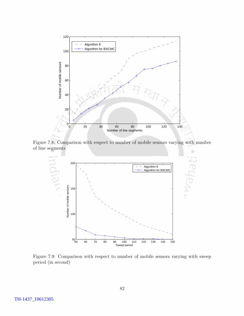
0 20 40 60 80 100 120 1400
20
40
60
80
100
120
Number of line segments
Num
ber
of m
obile
sen
sors
Algorithm 8Algorithm for BSCMC
Figure 7.8: Comparison with respect to number of mobile sensors varying with numberof line segments
50 60 70 80 90 100 110 120 130 140 15050
100
150
200
Sweep period
Num
ber
of m
obile
sen
sors
Algorithm 8Algorithm for BSCMC
Figure 7.9: Comparison with respect to number of mobile sensors varying with sweepperiod (in second)
82
TH-1437_10612305

Sweep period Number of Mobile SensorsAlgorithm for BSCMC Algorithm 8
50 75 19760 67 17970 62 13580 58 11990 56 107100 54 97110 52 86120 51 77130 51 71140 50 66150 50 60
Table 7.2: Comparison of the number of mobile sensors to achieve sweep coverage varyingsweep period for fixed number of line segments
which is equal to 50. A graphical representation of the Table 7.2 is illustrated in Fig. 7.9.
Table 7.2 and Fig. 7.9 show that with increasing number of line segments, the difference
between the average number of mobile sensors decreases. In general the algorithm for
BSCMC performs better than Algorithm 8.
7.7 Conclusion
In this chapter, we have introduced sweep coverage concept for barriers. In barrier
sweep coverage, mobile sensors periodically visit all points of a set of finite curves.
For a single curve, we have solved the problem optimally. Energy utilization for the
mobile sensors is restricted as they are battery-powered. Considering the limitation,
an energy restricted barrier sweep coverage problem is defined for a finite curve. A 133-
approximation algorithm is proposed to solve the problem. We have proved that finding
minimum number of mobile sensors to sweep cover a set of finite curves is NP-hard
and cannot be approximated within a factor of 2, unless P=NP. We have proposed a 5-
approximation algorithm to solve the problem. A 2-approximation algorithm is proposed
for a special case of the problem. As an application of barrier sweep coverage, we have
defined a data gathering problem with data mules. A 3-approximation algorithm is
proposed to solve the problem.
83
TH-1437_10612305

TH-1437_10612305

Chapter 8
Distributed Sweep Coverage
8.1 Introduction
Li et al. [41] comments on the impossibility of designing distributed sweep coverage
algorithm for a given set of PoIs. An individual mobile sensor cannot have knowledge of
the movement paths of all other mobile sensors without global information. Therefore, a
mobile sensor cannot locally say “yes” or “no” to the question of whether a given set of
PoIs is globally sweep covered. In this chapter, we propose a distributed sweep coverage
algorithm in a different context. We assume static sensors are placed at the location of
PoIs, one for each. The set of static sensors form a connected network. A set of mobile
sensors visits the static sensors once in a given time period to sweep cover the static
sensors. In this setting topology of the underlying network may change due to failure
or addition of the static sensors. But it is not possible to apply sequential Algorithm 2
(chapter 3) for every change in network topology. In this scenario distributed solution
of the sweep coverage plays an important role. The static sensors themselves decide the
positions and movement strategy of the mobile sensors by some distributed coordina-
tions. There are several applications in data gathering, where a set of mobile sensors
periodically visits the static sensors to collect and/or exchange data. This periodic visit
is important because the static sensors may not have sufficient memory for frequent
sampling and storing the data in its memory. Another reason for periodic visit might
be for updating sensing instructions.
85
TH-1437_10612305

Definition 8.1.1 (Distributed sweep coverage problem). Let U = {u1, u2, · · · , un} be
the set of PoIs in a two dimensional plane and S = {s1, s2, · · · , sn} be the set of static
sensors such that si is located at ui for all i = 1 to n. Let M = {m1, m2, · · · , mn} be the
set of mobile sensors with uniform speed v. For a given t > 0, S finds minimum number
of mobile sensors with their positions such that each PoI in U is t-sweep covered.
8.1.1 Contribution
• We introduce a distributed sweep coverage problem and propose a 4-approximation
algorithm as a solution.
• A 2-approximation algorithm is also proposed for a special case.
8.2 Approximation for a Special Case of Distributed
Sweep Coverage
We first propose a distributed algorithm for a special case of the problem where each
mobile sensor visits all static sensors. Then solution for the distributed sweep coverage
problem is proposed, where each mobile sensor does not necessarily visit all static sensors.
8.2.1 System Model and Algorithm
Let n static sensors with unique id ∈ {0, 1, 2, · · · , n − 1} and communication range
rc are placed at all PoIs. Two static sensors are neighbor of each other if they are
within a distance rc. Let Gc = (U,Ec, w) be the connected communication graph, where
each static sensor i is a vertex and (i, j) is the edge between two neighbors i and j.
Edge weight w(i, j) for the edge (i, j) is the Euclidian distance between i and j. Let
G = (U,E, w) be the corresponding complete graph of Gc. For any subgraph H of G,
we write w(H) for the sum of the edge weights of H . Let t be the sweep period of every
static sensor. All mobile sensors can move with uniform speed v. Every static sensor
uses control message for finding Euler tour by marking the edges and the positions of the
mobile sensors by marking the point on the edges. There is an initiator, static sensor
86
TH-1437_10612305

s for initiating the control message. Every static sensor maintains a variable status
for each edge incident on it, which can be either used or unused. An edge status:=
used means one control message for finding Euler tour has passed through the edge,
otherwise status:= unused. Based on the above discussion we propose Algorithm 10
(DistributedSweepCoverage).
Algorithm 10 DistributedSweepCoverage
1: Find a MST Tc of Gc by the distributed MST algorithm [24].2: Doubling every edge (i, j) ∈ Tc with same weight, one edge is (i, j) and other is (j, i).3: Initial status of each edge (i, j) ∈ Tc is unused4: Initiator s selects an unused edge (s, j) ∈ Tc, marks the edge for Euler tour and
assigns d = w(s, j). If b dvtc ≥ 1 then s calculates b d
vtc number of points on (s, j)
and marks them as positions of mobile sensors and sends < m, d− vt× b dvtc > to j.
Otherwise s sends a message < m, d > to j. The status of the edge (s, j) becomeused.
5: j executes following after receiving a message < m, d > from i.Choose an unused edge (j, k) ∈ Tc other than (j, i) and marks the edge for Eulertour. Now d = d + w(j, k). If b d
vtc ≥ 1, calculates b d
vtc number of points on (j, k)
and marks them as positions of mobile sensors and sends < m, d− vt× b dvtc > to k.
Otherwise j sends a message < m, d > to k. The status of the edge (j, k) becomeused. If no such unused edge (j, k) ∈ Tc other than (j, i) exists then j executes step5 for the edge (j, i).
6: When the message < m, d > returns back to the initiator s and every edge in Tc
incident to s is used, and if d > 0, the s marks its position for a mobile sensor.
The Algorithm 10 returns marked edges for Euler tour and corresponding marked
points for placement of mobile sensors. The mobile sensors start moving along the edges
of the Euler tour at the same time once they all are placed. The movement of all mobile
sensors guarantee sweep coverage for all the PoIs. Following theorems give correctness
and approximation factor of the algorithm.
Theorem 8.2.1. Let T be a minimum spanning tree of G and Tc be the minimum
spanning tree of Gc. Then w(T ) = w(Tc).
Proof. Clearly, w(T ) ≤ w(Tc). For all the edges e ∈ E(Gc) implies w(e) ≤ rc, since rc is
the communication range. Therefore, e ∈ E(Tc) implies w(e) ≤ rc. Now let us consider
the following two cases:
Case 1: All edges of T are with weight ≤ rc. T is a spanning tree of Gc and therefore
87
TH-1437_10612305
w(Tc) = w(T ).
Case 2: There exist an edge e in T such that w(e) > rc. Let us consider the graph
Tc ∪ {e}. This graph must contains a cycle containing e and w(e) is greater than the
weights of all other edges of the cycle. So, by the cycle property of minimum spanning
tree, e cannot be a part of any MST of G, contradicting the fact that e is a part of T .
Hence w(e) ≤ rc and therefore, by case 1, w(Tc) = w(T ).
Theorem 8.2.2. Algorithm 10 produces approximation ratio 2 for finding minimum
number of mobile sensors.
Proof. Let Lopt be the optimal TSP tour on the corresponding complete graph G. If T is
an MST on G with cost w(T ), then one can easily prove w(T ) ≤ w(Lopt). Algorithm 10
computes an MST Tc on the graph Gc and by Theorem 8.2.1, w(Tc) = w(T ). Therefore,
w(Tc) ≤ w(Lopt). Let E be the Eulerian graph formed after doubling each edge of Tc.
Then w(E) ≤ 2w(Lopt). By Theorem 3.2.2, the approximation ratio of the Algorithm 10
is 2.
Theorem 8.2.3. Message complexity of the Algorithm 10 is O(n logn + |Ec|), where|Ec| is the number of edges in Ec.
Proof. Total number of messages required for finding number of mobile sensors and their
initial positions depends on the distributed construction of MST and finding Euler tour
by doubling each edge of the MST. The messages required to construct an MST by the
distributed algorithm [24] is O(n logn+ |Ec|). Total 2(n− 1) messages are required for
finding Euler tour by Algorithm 10, since in step 4 each static sensor sends one message
through all the tree edges which are incident on it. Therefore, messages complexity of
the algorithm is O(n logn+ |Ec|).
8.3 4-approximation Algorithm for Distributed Sweep
Coverage
In this section, we generalize the above Algorithm 10 to solve distributed sweep coverage
problem, where each mobile sensor does not necessarily visit all static sensors.
88
TH-1437_10612305

Let Tc be the minimum spanning tree computed in step 1 of the Algorithm 10. Now,
every static sensor removes all incident edges of Tc from its adjacency list which are of
length more than vt. This may split Tc into several connected components. Run the
remaining steps of Algorithm 10 for each of the components to find number of mobile
sensors and their initial positions.
To analyze the approximation factor of the proposed algorithm, we construct a com-
plete graph G′ = (U,E, w′) from the complete graph G = (U,E, w), where weight func-
tion w′ of G′ is defined as follows. For all e ∈ E, if w(e) ≤ vt then assign w′(e) = w(e)vt
,
otherwise assign w′(e) = 1. Let opt be the number of mobile sensor required in the op-
timal solution on the communication graph Gc and opt′ be the number of mobile sensor
required in the optimal solution on G . Following lemma gives a lower bound of opt.
Lemma 8.3.1. dw′(Tc)e ≤ 2opt.
Proof. It is easy to observe that opt′ ≤ opt. Let us consider the movement of the mobile
sensors in the optimal solution on G. Let P1, P2, · · · , Popt′ be the movement paths of the
opt′ number of mobile sensors in a time interval [t0, t+t0]. Since a mobile sensor can move
at most vt distance during the time interval, no Pi contains any edge with weight more
that vt. Therefore, in G′, w′(Pi) =w(Pi)vt
≤ 1 and thus∑opt′
i=1 w′(Pi) ≤ opt′. Consider a
vertex vi ∈ Pi for all i = 1 to opt′. Let H ′ be the subgraph of G′ such that V (H ′) = U
and E(H ′) =⋃opt′
i=1 E(Pi)⋃
{(vj, vj+1)| j = 1 to opt′ − 1}. Note that H ′ is a spanning
tree of G′ and w′(H ′)=∑opt′
i=1 w′(Pi) +
∑opt′−1i=1 w′(vi, vi+1) ≤ opt′ + (opt′ − 1) ≤ 2opt′ − 1.
Since T is the minimum spanning tree of G, w′(T ) ≤ w′(H ′) ≤ 2opt′ − 1. Therefore,
dw′(T )e ≤ 2opt′. By Theorem 8.2.1, w′(Tc) = w′(T ), and hence dw′(Tc)e ≤ 2opt′ ≤2opt.
Theorem 8.3.2. The above algorithm is a 4-approximation algorithm.
Proof. Let N be the number of mobile sensors computed by the algorithm. In step 1
of the proposed algorithm, MST Tc is computed. After computing the tree Tc, all the
edges of weight more than vt are deleted from Tc. Let m be the number of deleted edges.
There are following two cases.
Case 1: At least one edge is deleted (m 6= 0). The tree Tc splits into m+ 1 connected
components C1, C2, · · · , Cm+1 in Gc. The corresponding tours T1, T2, · · · , Tm+1 are
89
TH-1437_10612305

computed after doubling the edges of each component. Total number of mobile
sensors needed is∑m+1
i=1
⌈
w(Ti)vt
⌉
≤∑m+1
i=12w(Ci)
vt+ (m+ 1), where w(Ti) = 2w(Ci).
Also, w′(Tc) =∑m+1
i=1w(Ci)vt
+m. Therefore,
N ≤m+1∑
i=1
2w(Ci)
vt+ (m+ 1)
≤m+1∑
i=1
2w(Ci)
vt+ 2m
≤ 2w′(Tc)
≤ 4opt by Lemma 8.3.1
Case 2: No edge is deleted (m = 0). Total number of mobile sensors in this case is
given by
N ≤ 2⌈
w(Tc)vt
⌉
= 2 dw′(Tc)e ≤ 4opt.
Therefore, from the above two cases, the algorithm is a 4-approximation algorithm.
8.4 Conclusion
In this chapter we have proposed a distributed sweep coverage algorithm, where static
sensors are placed at every point of interest. The mobile sensors move on the plane
according to their schedule and designated paths to sweep cover all static sensors. In
the distributed algorithm all static sensors communicate with their immediate neighbors
and collectively compute number of mobile sensors to guarantee sweep coverage of all
static sensors. The approximation factor of the algorithm is 4. A 2-approximation
algorithm is also proposed for a special case.
90
TH-1437_10612305

Chapter 9
Conclusion
Sweep coverage concept is recently introduced in the literature where periodic patrol
inspections are sufficient for a given set of points of interest by a set of mobile sen-
sors. In this thesis, we have investigated various types of sweep coverage problem such
as point sweep coverage, area sweep coverage, barrier sweep coverage, energy efficient
sweep coverage, energy restricted sweep coverage and distributed sweep coverage from
the theoretical point of view. In our solution of the sweep coverage problem we have
overcome a flaw of the previous solution [41] and proposed a 3-approximation algorithm
to solve this NP-hard problem where points are the vertices of a weighted graph. A 2-
approximation algorithm is proposed for a special case of the problem, which is the best
possible approximation factor of the problem. We have investigated the sweep coverage
problem in two different contexts of heterogeneity. In the first context, sweep periods of
the PoIs are different, and in the second context speeds of all mobile sensors are differ-
ent. There is a flaw of the previous solution [41] for the problem corresponding to the
first context. We have remarked on the flaw and proposed an O(log ρ)-approximation
algorithm for this generalized problem, where ρ = tmax
tmin, tmin and tmax are the minimum
and maximum sweep periods of the PoIs such that points are the vertices of a weighted
graph. We have proved that it is impossible to design any constant factor approximation
algorithm to solve the problem corresponding to the second context, unless P=NP. We
have introduced two variations of sweep coverage problem handling different types of
power issues of WSNs. Objective of the first problem is to guarantee sweep coverage for
91
TH-1437_10612305

a given set of PoIs by a set of static and/or mobile sensors with minimum energy con-
sumption per unit time. An 8-approximation algorithm is proposed to solve the problem.
Another solution for a special case is also proposed, which achieves the best possible ap-
proximation factor 2. Objective of the second problem is to find minimum number of
mobile sensors to guarantee sweep coverage where the maximum energy utilization by a
mobile sensor is bounded. for that, we have proposed a (5+ 2α)-approximation algorithm
to solve the problem. We have introduced area sweep coverage problem and proved that
the problem is NP-hard. Then a 2√2-approximation algorithm is proposed for a square
area. For arbitrary bounded region the approximation factor is a function of perimeter
and area of the bounded region. We have introduced sweep coverage concept for barri-
ers, where the objective is to sweep cover finite curves in a plane. We have solved the
problem optimally for a single curve. To resolve the issue of limited battery power of
the mobile sensors, we have proposed a solution by introducing an energy source in the
plane. To solve the problem we have proposed a 133-approximation algorithm. We have
proved that finding minimum number of mobile sensors to sweep cover a set of finite
length curves is NP-hard and cannot be approximated within a factor of 2, unless P=NP.
Then we have proposed 5-approximation algorithm to solve it. For a special case of this
problem we have proposed a 2-approximation algorithm. As an application of barrier
sweep coverage, we have defined a data gathering problem with data mules, where the
concept of barrier sweep coverage is applied for gathering data by utilizing minimum
number of data mules. For that a 3-approximation algorithm is proposed to solve the
problem. We have introduced a distributed sweep coverage problem where static sen-
sors are placed at the location of the PoIs, one for each and for that a 4-approximation
algorithm is proposed to solve the problem.
Above algorithms can be applied for the class of coverage problems where coverage
requirement is time variant. We have designed several constant factor approximation
algorithms for various sweep coverage problems. There is a scope of further improvement
on the approximation factors of the above problems. In future, we want to investigate
some other issues such as fault tolerance, scalability, self-stabilization, etc. in the context
of sweep coverage. However designing online algorithm for sweep coverage might be a
nice extension for further study.
92
TH-1437_10612305

Bibliography
[1] Fadi M. Al-Turjman, Hossam S. Hassanein, and Mohamed A. Ibnkahla. Connectiv-
ity optimization for wireless sensor networks applied to forest monitoring. In Pro-
ceedings of the 2009 IEEE international conference on Communications, ICC’09,
pages 285–290, Piscataway, NJ, USA, 2009. IEEE Press.
[2] Giuseppe Anastasi, Marco Conti, and Mario Di Francesco. Data collection in sensor
networks with data mules: an integrated simulation analysis. In IN: PROC. OF
IEEE ISCC, 2008.
[3] Novella Bartolini, Tiziana Calamoneri, Emanuele G. Fusco, Annalisa Massini, and
Simone Silvestri. Push & pull: autonomous deployment of mobile sensors for a
complete coverage. Wireless Networks, 16(3):607–625, 2010.
[4] Maxim A. Batalin and Gaurav S. Sukhatme. Multi-robot dynamic coverage of a
planar bounded environment. In Technical Report, CRES-03-011, 2002.
[5] Llia Blin, Maria Potop-Butucaru, Stephane Rovedakis, and Sbastien Tixeuil. A new
self-stabilizing minimum spanning tree construction with loop-free property. In Idit
Keidar, editor, Distributed Computing, volume 5805 of Lecture Notes in Computer
Science, pages 407–422. Springer Berlin Heidelberg, 2009.
[6] Azzedine Boukerche, Richard Werner Nelem Pazzi, and Regina Borges Araujo.
Fault-tolerant wireless sensor network routing protocols for the supervision of
context-aware physical environments. Journal of Parallel and Distributed Com-
puting, 66(4):586 – 599, 2006. Algorithms for Wireless and Ad-Hoc Networks.
93
TH-1437_10612305
[7] Ionut Cardei and Mihaela Cardei. Energy efficient connected coverage in wireless
sensor networks. Int. J. Sen. Netw., 3(3):201–210, May 2008.
[8] M. Cardei, M.T. Thai, Yingshu Li, and Weili Wu. Energy-efficient target coverage
in wireless sensor networks. In INFOCOM 2005. 24th Annual Joint Conference of
the IEEE Computer and Communications Societies. Proceedings IEEE, volume 3,
pages 1976–1984 vol. 3, March 2005.
[9] Mihaela Cardei and Ding-Zhu Du. Improving wireless sensor network lifetime
through power aware organization. Wireless Networks, 11(3):333–340, 2005.
[10] Guner D. Celik and Eytan Modiano. Dynamic vehicle routing for data gathering
in wireless networks. In CDC, pages 2372–2377, 2010.
[11] Manju Chaudhary and Arun K. Pujari. High-energy-first (HEF) heuristic for
energy-efficient target coverage problem. CoRR, abs/1103.4769, 2011.
[12] Ai Chen, Santosh Kumar, and Ten H. Lai. Designing localized algorithms for
barrier coverage. In Proceedings of the 13th Annual ACM International Conference
on Mobile Computing and Networking, MobiCom ’07, pages 63–74, New York, NY,
USA, 2007. ACM.
[13] N. Christofides. Worst-case analysis of a new heuristic for the travelling salesman
problem. Technical Report 388, Graduate School of Industrial Administration,
Carnegie Mellon University, 1976.
[14] Hung-Chi Chu, Wei-Kai Wang, and Yong-Hsun Lai. Sweep coverage mechanism
for wireless sensor networks with approximate patrol times. Ubiquitous, Autonomic
and Trusted Computing, Symposia and Workshops on, 0:82–87, 2010.
[15] Jurek Czyzowicz, Leszek Gasieniec, Adrian Kosowski, and Evangelos Kranakis.
Boundary patrolling by mobile agents with distinct maximal speeds. In Camil
Demetrescu and MagnusM. Halldorsson, editors, Algorithms ESA 2011, volume
6942 of Lecture Notes in Computer Science, pages 701–712. Springer Berlin Heidel-
berg, 2011.
94
TH-1437_10612305
[16] Gautam K. Das, Robert Fraser, Alejandro Lopez-Ortiz, and Bradford G. Nickerson.
On the discrete unit disk cover problem. In WALCOM, pages 146–157, 2011.
[17] Dinesh Dash, Arijit Bishnu, Arobinda Gupta, and Subhas C. Nandy. Approximation
algorithms for deployment of sensors for line segment coverage in wireless sensor
networks. Wireless Networks, 19(5):857–870, 2013.
[18] Dinesh Dash, Arobinda Gupta, Arijit Bishnu, and Subhas C. Nandy. Line coverage
measures in wireless sensor networks. J. Parallel Distrib. Comput., 74(7):2596–2614,
2014.
[19] Junzhao Du, Yawei Li, Hui Liu, and Kewei Sha. On sweep coverage with minimum
mobile sensors. In Proceedings of the 2010 IEEE 16th International Conference on
Parallel and Distributed Systems, ICPADS ’10, pages 283–290, Washington, DC,
USA, 2010. IEEE Computer Society.
[20] Adrian Dumitrescu and Csaba D. Toth. Computational geometry column 59.
SIGACT News, 45(2):68–72, June 2014.
[21] S. Eidenbenz, C. Stamm, and P. Widmayer. Inapproximability results for guarding
polygons and terrains. Algorithmica, 31(1):79–113, 2001.
[22] Herbert Fleischner. Eulerian Graphs and Related Topics, volume 2. North Holland,
1991.
[23] D. W. Gage. Command control for many-robot systems. In Proc. 19th Annu. AUVS
Tech. Symp., AUVS-92,Hunstville AL, pages 22–24, June 1992.
[24] R. G. Gallager, P. A. Humblet, and P. M. Spira. A distributed algorithm for
minimum-weight spanning trees. ACM Trans. Program. Lang. Syst., 5(1):66–77,
January 1983.
[25] Naveen Garg. Saving an epsilon: a 2-approximation for the k-mst problem in
graphs. In Harold N. Gabow and Ronald Fagin, editors, Proceedings of the 37th
Annual ACM Symposium on Theory of Computing, Baltimore, MD, USA, May
22-24, 2005, pages 396–402. ACM, 2005.
95
TH-1437_10612305

[26] Subir Kumar Ghosh. Approximation algorithms for art gallery problems in poly-
gons. Discrete Applied Mathematics, 158(6):718–722, 2010.
[27] Dorit S. Hochbaum and Wolfgang Maass. Approximation schemes for covering and
packing problems in image processing and VLSI. J. ACM, 32(1):130–136, 1985.
[28] D. Karaboga and B. Basturk. On the performance of artificial bee colony (abc)
algorithm. Applied Soft Computing, 8(1):687 – 697, 2008.
[29] Dervis Karaboga and Bahriye Akay. A survey: algorithms simulating bee swarm
intelligence. Artificial Intelligence Review, 31(1-4):61–85, 2009.
[30] Dervis Karaboga, Beyza Gorkemli, Celal Ozturk, and Nurhan Karaboga. A com-
prehensive survey: artificial bee colony (abc) algorithm and applications. Artificial
Intelligence Review, 42(1):21–57, 2014.
[31] Dervis Karaboga, Celal Ozturk, Nurhan Karaboga, and Beyza Gorkemli. Artificial
bee colony programming for symbolic regression. Information Sciences, 209(0):1 –
15, 2012.
[32] Akitoshi Kawamura and Yusuke Kobayashi. Fence patrolling by mobile agents with
distinct speeds. Distributed Computing, 28(2):147–154, 2015.
[33] G.Y. Keung, Bo Li, and Qian Zhang. The intrusion detection in mobile sensor
network. Networking, IEEE/ACM Transactions on, 20(4):1152–1161, Aug 2012.
[34] Fedor A. Kolushev and Alexander A. Bogdanov. Multi-agent optimal path plan-
ning for mobile robots in environment with obstacles. In Proceedings of the Third
International Andrei Ershov Memorial Conference on Perspectives of System In-
formatics, PSI ’99, pages 503–510, London, UK, UK, 2000. Springer-Verlag.
[35] S. Kumar, Ten H. Lai, M.E. Posner, and P. Sinha. Optimal sleep-wakeup algo-
rithms for barriers of wireless sensors. In Broadband Communications, Networks
and Systems, 2007. BROADNETS 2007. Fourth International Conference on, pages
327–336, Sept 2007.
96
TH-1437_10612305
[36] Santosh Kumar, Ten H. Lai, and Anish Arora. Barrier coverage with wireless
sensors. In Proceedings of the 11th Annual International Conference on Mobile
Computing and Networking, MobiCom ’05, pages 284–298, New York, NY, USA,
2005. ACM.
[37] Liron Levin, Alon Efrat, and Michael Segal. Collecting data in ad-hoc networks
with reduced uncertainty. Ad Hoc Networks, 17:71–81, 2014.
[38] Liron Levin, Michael Segal, and Hanan Shpungin. Optimizing performance of ad-
hoc networks under energy and scheduling constraints. In WiOpt, pages 11–20,
2010.
[39] Jing Li, Ruchuan Wang, Haiping Huang, and Lijuan Sun. Voronoi-based coverage
optimization for directional sensor networks. Wireless Sensor Network, 1(5):417–
424, 2009.
[40] Lei Li, Baoxian Zhang, Xiaojun Shen, Jun Zheng, and Zheng Yao. A study on the
weak barrier coverage problem in wireless sensor networks. Computer Networks,
55(3):711 – 721, 2011.
[41] Mo Li, Wei-Fang Cheng, Kebin Liu, Yunhao Liu, Xiang-Yang Li, and Xiangke Liao.
Sweep coverage with mobile sensors. IEEE Trans. Mob. Comput., 10(11):1534–1545,
2011.
[42] Benyuan Liu, Olivier Dousse, Jie Wang, and Anwar Saipulla. Strong barrier cov-
erage of wireless sensor networks. In Proceedings of the 9th ACM International
Symposium on Mobile Ad Hoc Networking and Computing, MobiHoc ’08, pages
411–420, New York, NY, USA, 2008. ACM.
[43] Jun Lu, Jinsu Wang, and T. Suda. Scalable coverage maintenance for dense wireless
sensor networks. In Sensor and Ad Hoc Communications and Networks, 2006.
SECON ’06. 2006 3rd Annual IEEE Communications Society on, volume 2, pages
651–660, Sept 2006.
[44] Ming Ma and Yuanyuan Yang. Adaptive triangular deployment algorithm for unat-
tended mobile sensor networks. IEEE Trans. Computers, 56(7), 2007.
97
TH-1437_10612305
[45] S. Mini, Siba K. Udgata, and Samrat L. Sabat. Artificial bee colony based sensor
deployment algorithm for target coverage problem in 3-d terrain. In Raja Natarajan
and Adegboyega K. Ojo, editors, Distributed Computing and Internet Technology
- 7th International Conference, ICDCIT 2011, Bhubaneshwar, India, February 9-
12, 2011. Proceedings, volume 6536 of Lecture Notes in Computer Science, pages
313–324. Springer, 2011.
[46] Christos H. Papadimitriou and Kenneth Steiglitz. On the complexity of local search
for the traveling salesman problem. SIAM J. Comput., 6(1):76–83, 1977.
[47] Maria Potop-Butucaru, Michel Raynal, and Sebastien Tixeuil. Distributed comput-
ing with mobile robots: An introductory survey. 2013 16th International Conference
on Network-Based Information Systems, 0:318–324, 2011.
[48] R. Ravi, Ravi Sundaram, Madhav V. Marathe, Daniel J. Rosenkrantz, and S. S.
Ravi. Spanning trees short or small. In Daniel Dominic Sleator, editor, Proceedings
of the Fifth Annual ACM-SIAM Symposium on Discrete Algorithms. 23-25 January
1994, Arlington, Virginia., pages 546–555. ACM/SIAM, 1994.
[49] A. Saipulla, C. Westphal, Benyuan Liu, and Jie Wang. Barrier coverage of line-
based deployed wireless sensor networks. In INFOCOM 2009, IEEE, pages 127–135,
April 2009.
[50] Anwar Saipulla, Benyuan Liu, Guoliang Xing, Xinwen Fu, and Jie Wang. Barrier
coverage with sensors of limited mobility. In Proceedings of the Eleventh ACM
International Symposium on Mobile Ad Hoc Networking and Computing, MobiHoc
’10, pages 201–210, New York, NY, USA, 2010. ACM.
[51] Anwar Saipulla, Cedric Westphal, Benyuan Liu, and Jie Wang. Barrier coverage
with line-based deployed mobile sensors. Ad Hoc Networks, 11(4):1381 – 1391, 2013.
[52] Mana Saravi and Bahareh J. Farahani. Distance constrained deployment (DCD)
algorithm in mobile sensor networks. In Proceedings of the 2009 Third International
Conference on Next Generation Mobile Applications, Services and Technologies,
NGMAST ’09, pages 435–440, Washington, USA, 2009. IEEE Computer Society.
98
TH-1437_10612305

[53] Rahul C. Shah, Sumit Roy, Sushant Jain, and Waylon Brunette. Data mules:
modeling and analysis of a three-tier architecture for sparse sensor networks. Ad
Hoc Networks, 1(2-3):215–233, 2003.
[54] Changxiang Shen, Weifang Cheng, Xiangke Liao, and Shaoliang Peng. Barrier
coverage with mobile sensors. In Parallel Architectures, Algorithms, and Networks,
2008. I-SPAN 2008. International Symposium on, pages 99–104, May 2008.
[55] Li Shu, Ke-wei Cheng, Xiaowen Zhang, and Jiliu Zhou. Periodic sweep coverage
scheme based on periodic vehicle routing problem. JNW, 9(3):726–732, 2014.
[56] S. Skiena. Grid graphs. in Implementing Discrete Mathematics: Combinatorics and
Graph Theory with Mathematica Reading, MA: Addison-Wesley, 1990.
[57] S. Slijepcevic and M. Potkonjak. Power efficient organization of wireless sensor
networks. In Communications, 2001. ICC 2001. IEEE International Conference
on, volume 2, pages 472–476 vol.2, 2001.
[58] James A. Storer and John H. Reif. Shortest paths in the plane with polygonal
obstacles. J. ACM, 41(5):982–1012, 1994.
[59] Javad Akbari Torkestani. An adaptive energy-efficient area coverage algorithm for
wireless sensor networks. Ad Hoc Networks, 11(6):1655 – 1666, 2013.
[60] Sabat S.L. Udgata, S.K. and S. Mini. Sensor deployment in irregular terrain using
artificial bee colony algorithm. In Nature Biologically Inspired Computing, 2009.
NaBIC 2009. World Congress on, pages 1309–1314, Dec 2009.
[61] Chao Wang and Huadong Ma. Data collection in wireless sensor networks by uti-
lizing multiple mobile nodes. In Mobile Ad-hoc and Sensor Networks (MSN), 2011
Seventh International Conference on, pages 83–90, Dec 2011.
[62] Guiling Wang, Guohong Cao, and T. LaPorta. A bidding protocol for deploying
mobile sensors. In Proceedings. 11th IEEE International Conference on Network
Protocols (ICNP 2003), pages 315 – 324, Nov. 2003.
99
TH-1437_10612305

[63] Guiling Wang, Guohong Cao, and Thomas F. LaPorta. Movement-assisted sensor
deployment. IEEE Trans. Mob. Comput., 5(6):640–652, 2006.
[64] Min Xi, Kui Wu, Yong Qi, Jizhong Zhao, Yunhao Liu, and Mo Li. Run to potential:
Sweep coverage in wireless sensor networks. In ICPP, pages 50–57, 2009.
[65] Guanqun Yang and Daji Qiao. Barrier information coverage with wireless sensors.
In INFOCOM, pages 918–926. IEEE, 2009.
[66] Meng Yang, Donghyun Kim, Deying Li, Wenping Chen, Hongwei Du, and Alade O.
Tokuta. Sweep-coverage with energy-restricted mobile wireless sensor nodes. In Kui
Ren, Xue Liu, Weifa Liang, Ming Xu, Xiaohua Jia, and Kai Xing, editors, WASA,
volume 7992 of Lecture Notes in Computer Science, pages 486–497. Springer, 2013.
[67] Azadeh Zamanifar, Mohsen Sharifi, and Omid Kashefi. A hybrid approach to actor-
actor connectivity restoration in wireless sensor and actor networks. In Robert
Bestak, Laurent George, Vladimir S. Zaborovsky, and Cosmin Dini, editors, The
Eighth International Conference on Networks, ICN 2009, 1-6 March 2009, Gosier,
Guadeloupe, France, pages 76–81. IEEE Computer Society, 2009.
[68] Chao Zhai and Yiguang Hong. Sweep coverage algorithm and coverage time estima-
tion for multi-agent systems. In Control and Decision Conference (CCDC), 2012
24th Chinese, pages 133–138, May 2012.
[69] Dimitrios Zorbas, Dimitris Glynos, Panayiotis Kotzanikolaou, and Christos
Douligeris. Solving coverage problems in wireless sensor networks using cover sets.
Ad Hoc Networks, 8(4):400–415, 2010.
100
TH-1437_10612305

Publication from the Contents of the Thesis
Papers published/submitted in International Journals:
[J1 ] Barun Gorain and Partha Sarathi Mandal, “Approximation Algorithm for Sweep
Coverage on Graph”, Information Processing Letters (Elsevier), Vol. 115, Issue 9,
pp. 712-718, 2015.
[J2 ] Barun Gorain and Partha Sarathi Mandal, “Approximation Algorithms for Sweep
Coverage in Wireless Sensor Networks”, Journal of Parallel and Distributed Com-
puting (Elsevier), Vol. 74, Issue 8, pp. 2699-2707, August 2014.
[J3 ] Barun Gorain and Partha Sarathi Mandal, “Approximation Algorithms for Bar-
rier Sweep Coverage in Wireless Sensor Networks”, Journal of Parallel and Dis-
tributed Computing (Elsevier) (Submitted).
[J4 ] Barun Gorain and Partha Sarathi Mandal, “Solving Energy Issues for Sweep
Coverage in Wireless Sensor Networks”, Discrete Applied Mathematics (Elsevier),
(Submitted).
Papers Published in International Conference Proceedings:
[C1 ] Barun Gorain and Partha Sarathi Mandal, “Energy Efficient Sweep Coverage with
Mobile and Static Sensors” in Proc. of International Conference on Algorithms
and Discrete Applied Mathematics (CALDAM 2015), Lecture Notes in Computer
Science (LNCS-8959) (Springer-Verlag), IIT Kanpur, India, pp. 275-285, Feb 8-10,
2015.
[C2 ] Barun Gorain and Partha Sarathi Mandal, “Brief Announcement: Sweep Cov-
erage with Mobile and Static Sensors” in Proc. of 16th International Symposium
on Stabilization, Safety, and Security of Distributed Systems (SSS 2014), Lecture
Notes in Computer Science (LNCS-8756) (Springer-Verlag), Paderborn, Germany,
pp. 346-348, Sep 28 - Oct 1, 2014.
TH-1437_10612305
[C3 ] Barun Gorain and Partha Sarathi Mandal, “Line Sweep Coverage in Wireless Sen-
sor Networks” in Proc. 6th international conference on COMmunication System
& NETworks (COMSNET’14), (IEEE Xplore), Bangalore, India, January 7-10,
2014.
[C4 ] Barun Gorain and Partha Sarathi Mandal, “Point and Area Sweep Coverage in
Wireless Sensor Networks” in Proc. of 11th International Symposium on Modeling
and Optimization in Mobile, Ad Hoc, and Wireless Networks (WiOpt’13), (IEEE
Xplore), Tsukuba Science City, Japan, pp. 140-145, May 13-17, 2013.
Other Publications
[C5 ] Barun Gorain, Partha Sarathi Mandal and Sandip Das, “ Poster Abstract: Ap-
proximation Algorithm for Minimizing the Size of a Coverage Hole in Wireless Sen-
sor Networks” in in Proc. of 14th International Conference on Distributed Com-
puting and Networking (ICDCN’13), Lecture Notes in Computer Science (LNCS-
7730), (Springer-Verlag), TIFR, Mumbai, India, pp. 463-464, Jan 3-6, 2013.
[C6 ] Barun Gorain and Partha Sarathi Mandal, “Optimal Covering with Mobile Sen-
sors in an Unbounded Region” in in Proc. of 8th International Conference on
Wireless Communication and Sensor Networks (WCSN’12), Phitsanulok, Thai-
land, December 19-23, 2012.
102
TH-1437_10612305