minimizing fuel emissions by optimizing vessel schedules in liner shipping with uncertain port times

Transportation Research Part E 48 (2012) 863–880

Contents lists available at SciVerse ScienceDirect

Transportation Research Part E

journal homepage: www.elsevier .com/locate / t re

Minimizing fuel emissions by optimizing vessel schedules in linershipping with uncertain port times

Xiangtong Qi a, Dong-Ping Song b,⇑a Department of Industrial Engineering and Logistics Management, Hong Kong University of Science and Technology, Clear Water Bay, Kowloon, Hong Kongb International Shipping & Logistics Group, School of Management, University of Plymouth, Drake Circus, Plymouth PL4 8AA, UK

a r t i c l e i n f o

Article history:Received 22 September 2011Received in revised form 15 December 2011Accepted 7 February 2012

Keywords:Liner shippingFuel emissionShip schedulingUncertaintyStochastic optimization

1366-5545/$ - see front matter � 2012 Elsevier Ltddoi:10.1016/j.tre.2012.02.001

⇑ Corresponding author. Tel.: +44 1752 585630; fE-mail addresses: [email protected] (X. Qi), dongpin

a b s t r a c t

We consider the problem of designing an optimal vessel schedule in the liner shippingroute to minimize the total expected fuel consumption (and emissions) considering uncer-tain port times and frequency requirements on the liner schedule. The general optimalscheduling problem is formulated and tackled by simulation-based stochastic approxima-tion methods. For special cases subject to the constraint of 100% service level, we prove theconvexity and continuous differentiability of the objective function. Structural propertiesof the optimal schedule under certain conditions are obtained with useful managerialinsights regarding the impact of port uncertainties. Case studies are given to illustratethe results.

� 2012 Elsevier Ltd. All rights reserved.

1. Introduction

Emissions from maritime transport have been brought into attention increasingly in the last decade. International Mar-itime Organization (IMO) published two studies on green house gas (GHG) emissions from ships in 2000 and 2009, respec-tively (Skjølsvik et al., 2000; Buhaug et al., 2009). The second study provided a comprehensive and authoritative assessmentof the level of GHG emitted by ships in the world, and estimated that shipping emitted 1046 million tonnes of CO2 in 2007,which accounted for about 3.3% of the global emissions.

Container shipping has been one of the fastest growing sectors in the shipping industry in the past three decades andmay well continue its rapid growth in the future (MEPC, 2009; Fransoo and Lee, in press). It is reported that containershipsare by far the most important source of CO2 emissions in the shipping industry, in both absolute and per tonne-km terms(Psaraftis and Kontovas, 2009). Corbett et al. (2009) stated that CO2 emissions from containerships are 1.3, 2.2 and 2.5 timesgreater than those from bulk shipping, crude oil tankers, and general cargo ships, respectively. Therefore, reducing CO2

emissions is an essential issue for the container shipping industry in achieving its environmental sustainability. A fewstudies have been conducted to quantify the impact of operational measures such as speed reduction, berth schedulingand route re-engineering on fuel consumptions and CO2 emissions in container shipping, e.g., Corbett et al. (2009), Psaraftiset al. (2009), Fagerholt et al. (2010), Golias et al. (2010), Cariou (2011), Lee et al. (2012), Meng and Wang (2011), Du et al.(2011), and Song and Xu (2012).

From the economic perspective, the steep increase in oil prices in the past several years has pressed the shipping com-panies to adopt fuel-cutting strategies. As fuel consumption of a ship is typically a cubic function of sailing speed (e.g. Ronen,

. All rights reserved.

ax: +44 1752 [email protected] (D.-P. Song).

http://dx.doi.org/10.1016/j.tre.2012.02.001

mailto:[email protected]

mailto:[email protected]

http://dx.doi.org/10.1016/j.tre.2012.02.001

http://www.sciencedirect.com/science/journal/13665545

http://www.elsevier.com/locate/tre

864 X. Qi, D.-P. Song / Transportation Research Part E 48 (2012) 863–880

1982; Fagerholt et al., 2010), many operational strategies are directly linked to reducing ship speeds. For example, slowsteaming has become a popular practice and been adopted by many shipping companies since 2008 (www.ci-online.co.uk).Since emissions from ships are proportional to the fuel consumption (e.g. Buhaug et al., 2009), slower speeds are generallyregarded as both economically and environmentally beneficial.

Christiansen et al. (2004, 2007) provided a comprehensive review of the research on ship routing and scheduling and clas-sified the literature into three categories: industrial shipping, tramp shipping, and liner shipping. Liner shipping has its un-ique characteristics, e.g., ships are usually deployed on a closed route with weekly frequency following a published scheduleof sailings with a fixed port rotation, and laden/empty containers are loaded on/off the ships at each port-of-call (Song et al.,2005; Ronen, 2011). Quite a few authors have addressed the economic aspects (e.g. profit, capital investment, and operatingcosts) of the vessel routing and deployment in the liner shipping, e.g. Rana and Vickson (1991), Cho and Perakis (1996),Powell and Perakis (1997), Ting and Tzeng (2003), Shintani et al. (2007), Agarwal and Ergun (2008), Karlaftis et al. (2009),Notteboom and Vernimmen (2009), Alvarez (2009), Meng and Wang (2010), Wang and Meng (2011a,b), and Ronen(2011). However, as pointed out by Christiansen et al. (2007) and Ronen (2011), relatively little research has been publishedregarding optimizing the speed of vessels. Fagerholt et al. (2010) developed a shortest path approach to minimize fuel con-sumption (or emissions) by optimizing ship speed in deterministic fixed shipping routes subject to time window for the startof service at each port. Ronen (2011) analyzed the trade-off between speed reduction and adding vessels to a container linerroute using a cost model. Meng and Wang (2011) determine service frequency, ship fleet deployment plan, and sailingspeeds for a long-haul liner service route by minimizing average daily operating cost.

Uncertainty is another important characteristic in liner shipping, which may exist in equipment availability, sea transportlegs or container ports due to various reasons such as congestion, uncertain handling time, and weather condition. For exam-ple, Cheung and Chen (1998) considered the uncertainties in container supplies, demands, and vessel capacity and their im-pact on empty container repositioning. A survey on the sources of schedule unreliability in the East Asia – Europe route forthe fourth quarter of 2004 revealed that port/terminal congestion (unexpected waiting times before berthing or before start-ing loading/discharging) accounted for 65.5%, port/terminal productivity below expectations (loading/discharging) ac-counted for 20.6%, and unexpected waiting times in port channel access (pilotage, towage) accounted for 4.7%(Notteboom, 2006). Because of the cumulative effect, a delay at one port-of-call may cause delays at the rest of port-of-callsin the service route unless there are some mechanisms implemented to reduce port times (e.g. cut a port-of-call) or reducesea times (e.g. increase vessel speed) to make up the lost time. It was reported that the vessel arrival reliability with respectto the published schedule could be as low as 50% for many service routes (Notteboom, 2006; Vernimmen et al., 2007).Clearly, uncertainty will impact on the vessel’s reliability, fuel consumption and emissions, particularly in situations if theschedules were not well designed. For example, for a weekly service with ten vessels deployed, the round-trip journey timewill be fixed at 70 days. For any vessel, if more time is scheduled to some legs, less time will be allocated to other legs. A portdelay before a tight leg may force the vessel to sail at the maximum speed in order to respect the schedule, but the vesselcould still fail to reach the next port on time, resulting in a deteriorate service level. Here a vessel’s service level refers to theprobability that the vessel is able to arrive at a port no later than the published planned arrival time. The delayed vessel ar-rival at a port may impact on berth allocation and handling operations, which may further influence downstream supplychain members’ operations (e.g. inland transportation operators’ truck scheduling, customers’ inventory management). Poorvessel service level could lead to dissatisfaction of shippers and damage liners’ reputation. Therefore, when designing theliner service schedules in advance, it is important to take into account the uncertainties in the system so that a reasonablyhigh service level can be achieved.

In the literature, the majority of the above research on vessel routing, scheduling and deployment has not explicitly con-sidered the stochastic aspect of the systems. This paper attempts to fill this research gap. Since port-related uncertainty is thedominant source of vessel schedule unreliability (Notteboom, 2006), we will concentrate on the port time uncertainty. Morespecifically, this study focuses on designing an optimal vessel schedule in a given shipping route with the aim to minimizethe total fuel consumption (or emissions) by considering uncertain port times at each port-of-call and the frequency require-ments on the liner schedule. Meanwhile, by introducing the penalty of being late, we are able to design an optimal vesselschedule with reasonably high service levels.

The remainder of the paper is organized as follows. The next section formulates the problem. The section after examinesthe optimal schedule and its structural properties for special cases with 100% service levels, as well as the stochastic approx-imation approach for the general case. Next we provide numerical studies to demonstrate the results, followed byconclusions.

2. The model and service level

Liner service differs from other shipping sectors mainly in its regularity. Usually, a set of vessels with similar sizes aredeployed to call at a fixed sequence of ports in the shipping route to provide a weekly service, where a round trip visit ofall port-of-calls is called a voyage. Vessels sail along the shipping route in consecutive voyages by following the publishedschedule, carrying containers over sea legs, and loading/unloading containers at port-of-calls. In order to describe thedynamics of the system, we introduce the following notation first.

http://www.ci-online.co.uk

X. Qi, D.-P. Song / Transportation Research Part E 48 (2012) 863–880 865

Notation

n
the number of voyages that a vessel sails along the service route in the planning horizon N the total number of port-of-calls in a single voyage T the journey time of a single voyage ni the vessel’s port time at the ith port-of-call It is a random variable subject to li 6 ni 6 ui
fi(.)
the probability distribution function of random variable ni
Fi(.)
the cumulative distribution function of random variable ni
di
the distance in nautical miles from the ith port-of-call to the (i+1)th port-of-call si the planned transit time from the ith port-of-call to the (i+1)th port-of-call, which is a decision variable ti,k the planned vessel arrival time at the ith port-of-call in the kth voyage ta
i;k
the actual vessel arrival time at the ith port-of-call in the kth voyage
tdi;k

the actual vessel departure time at the ith port-of-call in the kth voyage

si,k
the vessel sailing speed in knots in the leg from the ith port-of-call to the (i+1)th port-of-call in the kth voyage,which takes a value in [S0,S], where S0 is the minimum sailing speed and S is the maximum sailing speed
SLi,k
the service level at the ith port-of-call in the kth voyage, i.e. the probability that the vessel arrives at the ith port-of-call no later than the planned arrival time
gs(s)
the fuel consumption from the vessel at sea per nautical mile at sailing speed s
2.1. System dynamics

Due to the uncertainty at ports and constraints of vessel sailing speeds, a vessel may reach a port before or after theplanned arrival time. We assume that if a vessel arrives at a port earlier than the planned arrival time (the difference is calledearliness time), it does not affect the vessel’s port time. Namely, the earliness time does not form a part of the vessel’s porttime. The above assumption represents one type of practices/contracts between shipping lines and port/terminal operators,in which early arrived vessels have to wait until their time slot due to reasons such as the to-be-loaded containers or re-quired equipment are not ready until the planned vessel arrival time. A vessel’s departure time depends on its actual arrivaltime, planned arrival time, and the random port time at the current port. The randomness of the port time may be caused byloading/unloading uncertainty, congestion, availability of relevant equipment, and other factors. More specifically, the evo-lution of the system dynamics under a given planned schedule {si: i = 1, 2, . . ., N} can be described as follows (let s0 = 0),

s1 þ s2 þ � � � þ sN�1 þ sN ¼ T; ð1Þ

ti;k ¼ ðk� 1ÞT þXi�1

j¼1

sj; for k P 1 and 1 6 i 6 N þ 1; ð2Þ

ta1;1 ¼ t1;1; and ta

1;kþ1 ¼ taNþ1;k; for k P 1; ð3Þ

tai;k ¼

tdi�1;k þ di�1=S0 if ti;k > td

i�1;k þ di�1=S0

ti;k if tdi�1;k þ di�1=S 6 ti;k 6 td

i�1;k þ di�1=S0

tdi�1;k þ di�1=S ti;k < td

i�1;k þ di�1=S

8>><>>: ; for 2 6 i 6 N þ 1; ð4Þ

tdi;k ¼max ti;k; ta

i;k

n oþ ni for k P 1 and 1 6 i 6 N: ð5Þ

The above constraints (1) and (2) is the frequency requirement of a liner service to ensure its regularity. The problem is tofind the optimal {si: i = 1, 2, . . ., N} by minimizing the total expected fuel consumption in a voyage averaging over n consec-utive voyages in the planning horizon subject to conditions (1)–(5),

Min J ¼min E1n

Xn

k¼1

XN

i¼1

di � gsdi

taiþ1;k � td

i;k

!þ hi ta

i;k � ti;k

� �" #: ð6Þ

In the objective function (6) there are two cost terms. The delay cost function hi(.) is a non-decreasing function with hi(0) = 0.Physically, hi(.) penalizes the vessel delays, which represents the reality that if the vessel is too late it may be penalized forcontainers delay cost or good will loss to customers.

The fuel cost function gs(s) is the fuel consumption from the vessel at sea per nautical mile at sailing speed s. It is wellrecognized that the ship fuel consumption per unit of time has a cubic relationship with respect to the sailing speed, whereasthe emission is proportional to the fuel consumption (e.g. Corbett and Fischbeck, 1997; Corbett et al., 2009; Wang, 2010;Fagerholt et al., 2010). Therefore, the fuel consumption and the emission from a ship per nautical mile is a quadratic convexfunction with respect to the speed. For example, Fagerholt et al. (2010) provided an empirical formula for fuel consumptionper nautical mile in a quadratic format. In this paper, we follow the assumption that gs(s) is a quadratic convex function,


monotonic increasing, and positive in the meaningful speed interval including [S0,S]. However, our analysis, except for thenumerical studies, is actually valid for any convex and monotonic increasing functions, not necessarily for a quadraticfunction.

The general problem in (1)–(6) is difficult to solve analytically. Firstly, the objective function defined on the right-hand-side of (6) is obviously non-linear with respect to the decision variables and does not have a closed-form expression. Sec-ondly, since variables ta

i;k and tdi;k may depend on all the random variables in the set {njj1 6 j < i} for k = 1, and all the random

variables in the set {njj1 6 j 6 N} for k > 1, the coupling effect of multiple random variables makes it difficult to analyse themathematic expectation in the objective function. Thirdly, due to the max operation in (5), the objective function in (6) maybe not differentiable.

As we mentioned in the introduction section, in designing the schedule for a liner service, it is important to estimate thevessel’s ability to follow the planned schedule. We use the term, service level, to represent a vessel’s reliability to follow theschedule.

Definition 1. A vessel’s service level at the ith port-of-call is defined as the probability that the vessel arrives at the ith port-of-call no later than the planned arrival time, i.e.

SLi;k :¼ Prob tai;k 6 ti;k

n o; for k P 1 and 2 6 i 6 N þ 1:

Here SLN+1 represents the service level that the vessel returns to the starting port for the next voyage.The following proposition gives a recursive way to calculate the service levels for a given vessel schedule. The equation

implies that the delay at an earlier port may be propagated to all the following ports.

Proposition 1. For a given schedule {si:i = 1,2, . . . ,N}, the expected service levels at individual port-of-calls in the first voyage(k = 1) are given by:

SLi;1 ¼ SLi�1;1 � Fi�1ðti;1 � ti�1;1 � di�1=SÞ þ SLi�2;1 �Z ui�2

ti�1;1�di�2=S

Z ti;1�ti�2;1�xi�2�di�2=S�di�1=S

li�2

fi�1ðxi�1Þfi�2ðxi�2Þdxi�1dxi�2 þ � � �

þ SL1;1 �Z u1

t2;1�d1=S

Z u2

t3;1�x1�d1=S�d2=S� � �Z ui�2

ti�1;1�x1�d1=S��di�2=S

�Z ti;1�x1�d1=S�x2�d2=S��xi�2�di�2=S�di�1=S

li�1

fi�1ðxi�1Þ � � � f1ðx1Þdxi�1 � � �dx1

To make the narrative and discussion smooth, we put the proofs of all propositions in the Appendix with those straightfor-ward ones being simplified or omitted. The computational results for service levels will be reported in the numerical studies.

3. Optimal schedule and structural properties

Although the general problem (1)–(6) is complicated and difficult to solve analytically, under a certain set of conditions itis analytical tractable or possible to establish interesting structural properties of the optimal schedule. This section addressestwo special cases first, then the general case.

3.1. Deterministic port times

In the deterministic case with li = ui for all ports, we can establish the closed-form optimal solution as follows. In partic-ular, the assertion (iii) of Proposition 2 implies an optimal constant speed for all legs, which is mainly due to the convexity ofthe objective function.

Proposition 2. If ni is deterministic for i = 1, 2, . . ., N, then

(i) a feasible schedule with 100% service level at each port-of-call exists if and only ifPðui þ di=SÞ 6 T;

(ii) a feasible schedule with 100% service level and zero earliness time at each port-of-call exists if and only ifPðui þ di=SÞ 6 T 6

Pðui þ di=S0Þ; and

(iii) underPðui þ di=SÞ 6 T, the optimal schedule with 100% service level at each port-of-call is given by:

si ¼ ui þdiPN

1di

T �XN

1

ui

!for i ¼ 1;2; . . . ;N: ð7Þ

Physically,Pðui þ di=SÞ represents the sum of total port times and the minimum total sea times in a single voyage. Assertion

(i) indicates that if this number is less than the journey time T, a feasible schedule with 100% service level at each port-of-call


exists. The expressionPðui þ di=S0Þ represents the sum of total port times and the maximum total sea times in a single voy-

age. Assertion (ii) indicates that ifPðui þ di=S0Þ is greater than the journey time T, a schedule with zero earliness time at each

port-of-call exists. Assertion (iii) provides a closed-form of an optimal schedule if the existence condition for 100% servicelevel schedules is satisfied.

In the deterministic case, if T >Pðui þ di=S0Þ, then the vessel is sailing at its minimum speed in all legs. Clearly, the min-

imum fuel consumption from a vessel in a round-trip is equal to J ¼P

di � gsðS0Þ, and the vessel’s earliness time at leg i isgiven by: (si � ui) � di/S0.

3.2. Stochastic port times with 100% service level constraints

Liner service has been criticized for its low service level in terms of reliability (Notteboom, 2006; Vernimmen et al., 2007).The main reason is the uncertainties in the voyage (either at ports or at sea). However, if the schedule has been better de-signed, it is possible that the vessel can achieve 100% service level at all ports. This section will explore such special cases andproduce useful managerial insights for the schedule design. Under the 100% service level constraints, all voyages are thesame and no lateness penalty is incurred. Therefore, we can only focus on a single voyage in this section.

We first have a proposition that gives a sufficient condition for the existence of a vessel schedule with 100% service level.

Proposition 3. IfPðui þ di=SÞ 6 T, then an optimal schedule with 100% service level at each port-of-call exists and can be

determined by solving an optimization problem

min J ¼minXN

i¼1

Giðsi; li; ui;diÞ ð8Þ

where,

Giðsi; li;ui; diÞ ¼

R uili

digsdi

si�xi

� �fiðxiÞdxi ui þ di

S 6 si 6 max ui þ diS ; li þ

diS0

n odigsðS0ÞFi si � di

S0

� �þR ui

si�diS0

digsdi

si�xi

� �fiðxiÞdxi max ui þ di

S ; li þ diS0

n o< si 6 ui þ di

S0

digsðS0Þ si > ui þ diS0

8>>>><>>>>:

ð9Þ

subject to

si P ðui þ di=SÞ for any i; ð10ÞXN

1

si ¼ T: ð11Þ

Although the objective function Gi(si, li,ui,di) looks complicated, it has good properties. The following proposition character-izes its convexity, which is useful to find an optimal schedule with 100% service level.

Proposition 4. IfPðui þ di=SÞ 6 T, then: (i) Gi(si,li,ui,di) is convex and continuously differentiable with respect to si; and (ii) J is

convex and continuously differentiable with respect to si.

This proposition indicates that the optimization problem in Proposition 3 can be solved using non-linear programmingmethods and a global optimal solution exists, because the constraints (10) and (11) are linear functions (Bradley et al.,1977). Many existing tools could be used to solve the above optimization problem, e.g. the Matlab tool fmincon (Venkatar-aman, 2009).

The following proposition discusses the possible existence of earliness time at any port in a schedule with 100% servicelevel.

Proposition 5.

(i) IfPðui þ di=SÞ 6 T, and ui � li 6 di(1/S0 � 1/S), then there exist feasible schedules with 100% service level at each port-of-

call and zero earliness time at the (i+1)th port-of-call.(ii) If

Pðui þ di=SÞ 6 T, and ui � li > di(1/S0 � 1/S), then any feasible schedule with 100% service level has a positive probability

of having non-zero earliness time at the (i+1)th port-of-call.

Recall that we assume the port time at a port i is bounded by an interval [li,ui]. The following proposition indicates that, tofind an optimal schedule with 100% service level, we can actually assume li = 0 for any port, without loss of any generality.

Proposition 6. The optimization problem in Proposition 3 is equivalent to finding the optimal solution s0i : i ¼ 1;2; . . . ;N� �

to,

minXN

i¼1

Gi s0i;0;ui � li;di� �


Subject to

s0i P ðui � li þ di=SÞ;XN

1

s0i ¼ T �XN

1

li

!:

Namely, si ¼ s0i þ li for any i.Proposition 6 indicates that we can assume all the lower bounds of port times being zero, i.e. li = 0 for any i, since the

solution to the original problem in Proposition 3 can be obtained by appropriately shifting the schedule of Proposition 6.In the remainder of this section, li will be regarded as 0 for any i unless explicitly specified. This will simplify our analysis.

The following Propositions 7 and 8 are our main results that characterize the structural properties of an optimal schedulewith 100% service level.

Proposition 7. IfPðui þ di=SÞ 6 T, and ni and nj are identical independent distributions, then the optimal schedule

s�i : i ¼ 1;2; . . . ;N� �

determined by Proposition 3 satisfies:

(i) if s�i ¼ ðui þ di=SÞ and di P dj, then s�j ¼ ðuj þ dj=SÞ;(ii) if s�i P li þ di=S0 and di P dj, then s�j P li þ dj=S0; and

(iii) if s�i > ui þ di=S0, then s�j P ui þ dj=S0 for any j.

Regarding its business meaning, Proposition 7 implies that if all port times (excluding the deterministic lower bound part)follow the same distribution, then the shortest leg will first reach the binding points of the constraints caused by the max-imum speed or the minimum speed. In other word, the shortest leg is the most problematic leg when designing the optimalschedule to achieve 100% service level and minimize the fuel consumption within the speed constraints.

Proposition 8. IfPðui þ di=SÞ 6 T; ni and nj are identical independent distributions (excluding the deterministic lower bound

part), and the vessel is not always sailing at its slowest speed in the entire journey, then the optimal schedule s�i : i ¼ 1;2; . . . ;N� �

determined by Proposition 3 satisfies:

(i) if di = dj, then s�i ¼ s�j ;(ii) if di > dj, then s�i > s�j ; and

(iii) if di > dj, then di=s�i > dj=s�j .

Proposition 8 provides the following managerial insights. Under the assumption that two ports have identical indepen-dent distributions of port times (excluding the lower bound parts), then: (i) if their distances to the next port-of-call are thesame, then the optimal planned leg-transit times should be the same; (ii) the leg with longer distance should have a largerleg-transit times; and (iii) but the allocation of the optimal planned leg-transit time is disproportional to their distances, andin favor of the shorter leg. While assertions (i) and (ii) are easy to understand, assertion (iii) reveals that the same port uncer-tainty will have a more severe impact on a shorter leg than on a longer leg. The last assertion can be explained by the intu-ition that a longer leg has a higher opportunity to compensate the possible delays caused at previous ports by appropriatelyadjusting the vessel sailing speed; moreover, to compensate the same amount of delay, the shorter leg has to increase thevessel sailing speed more dramatically than the longer leg, which incurs more fuel consumption due to the non-linear rela-tionship between the fuel consumption and the speed.

In addition, if the port times (excluding their lower bound parts) follow the same distribution for all ports, and lets0i : i ¼ 1;2; . . . ;N� �

be the optimal solution to the problem in Proposition 6 and {si: i = 1,2, . . . ,N} be the optimal solutionto the original problem in Proposition 3, then from Proposition 8, we have: di=s0i ¼ di=ðsi � liÞ is strictly increasing in di.

3.3. Stochastic port times without 100% service level constraints

In a general situation with stochastic port times, we may not able to or attempt to design a schedule to achieve 100% ser-vice levels at each port-of-call. A reasonable assumption about the journey time T is

Pðli þ di=SÞ 6 T 6

Pðui þ di=SÞ for this

case. The first inequality ensures that the vessel would not have zero service level at each port-of-call; whereas the secondinequality implies that the vessel will not achieve 100% service level at all port-of-calls.

It should be pointed out that without the 100% service level constraint the delays at one port-of-call might be propagatedto the next port, and even to the next voyage. It is important to estimate what the maximum possible delays are and howthey propagate along the route. Let qi,k be the maximum possible delay of the vessel at the ith port-of-call in the kth voyage.The following result is easy to establish.

Proposition 9. (i) The sufficient and necessary conditions for a schedule {si: i = 1,2,. . . ,N} to have a service level greater than zerobut less than 100% at each port-of-call are li + di/S < si < ui + di/S for any i; (ii) Under a schedule with li+di/S < si < ui+di/S for any i,


the maximum delays to be propagated from one voyage to the next is a constantPðui þ di=SÞ � T. More specifically, the maximum

possible delay of the vessel at each port-of-call in each voyage is given by:

Table 1A summ

Prop

Prop

Prop

Prop

Prop

Prop

Prop

Prop

Prop

Prop

q1;k ¼ qN;k�1 þ ðu1 þ d1=S� s1Þ; for 1 6 k; and qN;0 ¼ 0;

qi;k ¼ qi�1;k þ ðui þ di=S� siÞ; for 2 6 i 6 N and 1 6 k:

The problem in (1)–(6) is a general constrained stochastic optimization problem. It is complicated and difficult to solve
analytically. However, a simulation-based stochastic approximation approach can be used to optimize the schedule.
The following describes the stochastic approximation algorithm to optimize a set of parameters (more details can be re-ferred to Rubinstein, 1986; Fu and Hu, 1997). Let s := (s1,s2, . . . ,sN�1)T be a set of parameters to be optimized, and J(s) denotethe objective function. In our case, s represents the parameterized schedule and J(s) represents the fuel consumption definedin (6) under a given schedule s. The general form of the stochastic approximation is:

snþ1 ¼ sn � cn � rJn; ð12Þ

where sn is the parameter vector at the beginning of iteration n, rJn is an estimator of the gradient rJ(sn) (which is definedas r J(sn) := (@J(sn)/@s1,@J(sn)/@s2, . . . ,oJ(sn)/@sN�1)T), and cn is a positive sequence of step sizes such that (a) it decreases tozero, (b) the sum of all the sequence {cn} is infinite, and (c) the sum of its squares is bounded. Typically, the harmonic se-quence 1/n satisfies all above assumptions for cn.

When rJn is an unbiased estimator of the gradient rJ(sn), the above stochastic approximation (12) is called a Robbins-Monro (RM) algorithm; and when a finite difference estimator is used, it is called a Kiefer-Wolfowitz (KW) algorithm(Rubinstein, 1986). RM algorithms generally have faster convergence rates than the KW algorithms, but require direct mea-surements of the gradients (Kleinman et al., 1999). In this paper, we use the KW-type algorithm due to its simplicity. Thegradient estimator is obtained by averaging over 1000 samples via simulation. It should be pointed out that more efficientstochastic approximation algorithms could be developed, e.g. using perturbation analysis or other efficient gradient estima-tion techniques (c.f. Song and Sun, 1998; Kleinman et al., 1999; Marbach and Tsitsiklis, 2001).

Because our problem is a constrained optimization problem, several adjustments are introduced in the iterative searchprocedure. Firstly, the changes to {si} must ensure the design constraint, i.e. s1 + s2 + � � � + sN = T. Secondly, we impose a lowerbound constraint to si when it is updated, i.e. siP li+di/S. This is due to the fact that if si6 li+di/S, then the vessel will never beable to arrive at the next port-of-call on-time, which is unrealistic at the design stage (in which case more vessels should bedeployed to avoid such situation). Thirdly, we also impose an upper bound constraint to si when it is updated, i.e. si6 ui+di/S0.This is due to the fact that if siP ui+di/S0, then the vessel will definitely arrive at the next port-of-call before the scheduledtime. Therefore, further increasing the planned time for this leg would gain nothing. The above constraints are handled asfollows in our experiments.

ary of propositions’ roles and outcomes.

osition Roles and outcomes

Service level of a given liner service scheduleosition 1 It provides a formula to compute the expected service levels at individual port-of-calls in the first voyage

When port times are deterministicosition 2 It provides: (i) the necessary and sufficient conditions for the existence of a feasible schedule with 100% service level at each port-of-

call; (ii) the necessary and sufficient conditions for the existence of a feasible schedule with 100% service level and zero earlinesstime at each port-of-call; (iii) a closed-form of the optimal schedule with 100% service level

When port times are stochastic and focus on schedules with 100% service levelosition 3 It gives a sufficient condition for the existence of a vessel schedule with 100% service level. The optimal 100% service level schedule

can be obtained by solving a constrained optimization problemosition 4 It states that the objective function in Proposition 3 is convex and continuously differentiable. This indicates that a unique global

optimal solution exists, which can be obtained using well-developed non-linear programming methodsosition 5 It provides conditions to judge whether there exists earliness time at any port-of-call for a schedule with 100% service level. The

earliness time should be avoided if possible in order to minimize total fuel consumptionosition 6 It simplifies the constrained optimization problem in Proposition 3. The original problem is equivalent to a simpler one with zero

lower bounds of port times. That means, we only need concentrate on the uncertain part of port timesosition 7 It provides a set of structural properties of an optimal schedule. If the uncertain parts of port times at two ports follow the identical

independent distribution, then the optimal planned leg-transit time corresponding to the shorter leg must satisfy a constraintincurred by the longer leg

osition 8 It provides another set of structural properties of an optimal schedule. If the uncertain parts of port times at two ports follow theidentical independent distribution, then the optimal planned leg-transit time corresponding to the shorter leg must not be greaterthan the one corresponding to the longer leg. However, the allocation of the optimal planned leg-transit time is disproportional totheir distances, and in favor of the shorter leg

When port times are stochastic and focus on schedules without 100% service levelosition 9 It provides: (i) the necessary and sufficient conditions for a schedule to have a service level greater than zero but less than 100% at

each port-of-call; (ii) under the above conditions, a set of formula to compute the maximum possible delays of the vessel at eachport-of-call in each voyage


Note that the above constraints indicates that there are N � 1 independent control parameters (e.g. s1,s2, . . . ,sN�1) to beoptimized subject to li + di/S 6 si 6 ui + di/S0 for i = 1, 2, . . ., N � 1. The control parameter sN can be implicitly determined bysN = T � (s1 + s2 + � � � + sN�1). At the nth iteration, let sn,i denote the ith control parameter in vector s, and Dn,i denote thechange to be made on the ith element of the vector s in (12), i.e. (Dn,1,Dn,2, . . . ,Dn,N�1)T := �cn � rJn. If Dn,i is greater than zero,it will be upper bounded by ui+di/S0 – sn,i; On the other hand, if Dn,i is less than zero, it will be lower bounded by li+di/S –sn,i.This ensures that li+di/S 6 sn+1,i6 ui+di/S0 for i = 1, 2, . . ., N � 1. Finally, we set sN+1, i = T � (sn+1,1 + sn+1,2 + � � � + sn+1,N�1). Theiterative search procedure will be terminated if it reaches the pre-specified maximum number of iterations or there is noimprovement of solutions for a pre-specified number of iterations consecutively.

Although we are unable to establish the structural properties for the general cases analytically, we will use a range ofnumerical examples to explore whether the main analytical results in Proposition 8 derived from special cases can carry overto more general situations.

To have a comprehensive overview of the analytical results stated in the above propositions, we summarize the roles andmain outcomes of each proposition in Table 1.

4. Numerical studies

We have conducted numerical studies to validate our models and analysis. The purposes are three fold. First, we confirmthe main analytical findings for the special cases with 100% service level, and provide the simulation-based stochasticapproximation solutions for general cases without 100% service level constraints. Second, we evaluate the fuel savings ofour approach relative to alternative solutions, especially for cases with larger degree of uncertainties. Third, we examinethe impact on service levels when trying to reduce the fuel consumption and emissions, which will help us understandthe trade-off between them.

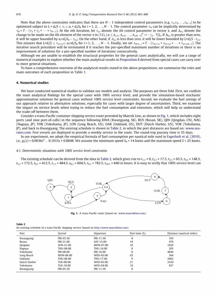
Consider a trans-Pacific container shipping service route provided by Maersk Line, as shown in Fig. 1, which includes eightports (and nine port-of-calls) in the sequence following KWA (Kwangyang, SK), BUS (Busan, SK), QIN (Qingdao, CN), NAG(Nagoya, JP), YOK (Yokohama, JP), LON (Long Beach, US), OAK (Oakland, US), DUT (Dutch Harbor, US), YOK (Yokohama,JP), and back to Kwangyang. The existing schedule is shown in Table 2, in which the port distances are based on: www.sea-rates.com. Five vessels are deployed to provide a weekly service in the route. The round-trip journey time is 35 days.

In our experiment, we adopt the empirical formula of fuel consumption per nautical mile used in Fagerholt et al. (2010),i.e., gs(s) = 0.0036s2 � 0.1015s + 0.8848. We assume the minimum speed S0 = 14 knots and the maximum speed S = 25 knots.

4.1. Deterministic situations with 100% service level constraints

The existing schedule can be derived from the data in Table 2, which gives rise to t1,1 = 0, t2,1 = 17.5, t3,1 = 65.5, t4,1 = 148.5,t5,1 = 172.5, t6,1 = 412.5, t7,1 = 484.5, t8,1 = 604.5, t9,1 = 782.5, t10,1 = 840 in hours. It is easy to verify that 100% service level can

QINBUS

KWANAG

YOKDUT

OAK

LON

Fig. 1. A trans-Pacific route (based on: www.maerskline.com).

Table 2An existing schedule of a trans-Pacific shipping service (based on http://www.maerskline.com).

Port Arrival Departure Port time (h) Distance (nautical miles)

Kwangyang FRI-03:30 FRI-11:30 8 103Busan FRI-21:00 SAT-15:00 18 476Qingdao SUN-21:00 MON-07:00 10 1029Nagoya THU-08:00 THU-16:00 8 205Yokohama FRI-08:00 FRI-16:00 8 4844Long Beach MON-08:00 WED-03:00 43 364Oakland THU-08:00 THU-17:00 9 2062Dutch Harbor TUE-08:00 WED-05:00 21 2550Yokohama TUE-18:00 WED-04:00 10 837Kwangyang FRI-03:30 FRI-11:30 8

http://www.searates.com

http://www.searates.com

http://www.maerskline.com

http://www.maerskline.com


be achieved at each port. From Proposition 2, the optimal schedule is given by: s�i : i ¼ 1;2; . . . ;N� �

¼ f13:82; 44:91;

68:18; 19:59; 281:86; 63:58; 125:58; 165:17; 57:32g. The fuel consumption per vessel per round-trip is 3148.08 tonnes and2690.80 tonnes under the existing schedule and the optimal schedule respectively. This implies that the existing schedulewould be 16.99% more costly above the optimal schedule if there is no port uncertainty.

4.2. Stochastic situations with 100% service level constraints

To consider the uncertain port time, assume the lower bounds of port times at each port-of-call take the correspondingvalues of the port time in Table 2, and the uncertain parts of port times follow the same uniform distributions for all port-of-calls. Consider six scenarios with different levels of uncertainties of port times ranging from U(0,0) to U(0,20) so that we canobserve the sensitivity of the results with respect to the level of port uncertainty. It can be verified that

Pðui þ di=SÞ 6 T for

all scenarios, and hence a feasible schedule with 100% service level exists by Proposition 2. Let JDet denote the fuel consump-tion per vessel per round-trip under the schedule designed based on deterministic optimal solution with the uncertain porttime upper bound as the deterministic port time, i.e. si ¼ ui þ di � ðT �

PuiÞ=

Pdi, for i = 1, 2, . . ., N. Let JOpt correspond to the

optimal schedule designed from Proposition 3.Table 3 gives the fuel consumptions under three schedules (the optimal schedule based on Propositions 3 and 4 and a

non-linear programming tool, the deterministic schedule based on Proposition 2, and the company’s original schedule in Ta-ble 2) in six scenarios, in which the columns ‘% above’ are calculated by (JDet � JOpt)/JOpt ⁄ 100% and (JOrig � JOpt)/JOpt ⁄ 100% forthe deterministic schedule and the original schedule, respectively. When the upper bound of the uniform distribution isgreater than 4 h, the original schedule cannot achieve 100% service level therefore indicated by ‘NA’ in the table.

Table 3 shows that the deterministic schedule based on Proposition 2 appears to be reasonably good, less than 3% morecostly above the optimal schedule in all experimented scenarios, whereas the original schedule is significantly worse thanthe optimal schedule in two feasible scenarios. Comparing different scenarios, the fuel consumption is increasing signifi-cantly as the port time and its uncertainty increase. This evidences the importance of explicitly considering the uncertaintyin port times.

We now illustrate the structural property given by Proposition 8. For the optimal schedule s�i� �

, let s0i ¼ s�i � li. Tables 4and 5 give s0i

� �and di=s0i

� �for the six scenarios. Note that in the tables we arrange the columns in the increasing order of di,

the leg distances. It can be seen that both s0i and di=s0i are increasing as di increases. This confirms the results of Proposition 8(ii) and (iii). An interesting observation is that as the degree of uncertainties increases, di=s0i is decreasing for the legs withsmaller distances (e.g. i = 1, 4, 6, 2, 9, 3) but increasing for the legs with larger distances (e.g. i = 7, 8, 5). This can be explainedby the fact that the actual sailing speed for smaller legs is more sensitive to the uncertainty in port time.

4.3. Stochastic situations without 100% service level constraints

In this section, the simulation-based stochastic approximation is used to find the ‘optimal’ schedule. As stochastic approx-imation algorithms are local-search methods, there is no guarantee that the global optimal solution can be found. We set thetermination criteria being either the number of search iterations reaches 100 or the number of consecutive iterations with-out improvement exceeds 10. To reduce the impact of initial solutions and obtain a better solution, we perform the search

Table 3The fuel consumption (in tonnes) under three schedules with 100% service levels.

Port time (h) JOpt JDet % Above JOrig % Above

li + U(0,0) 2690.80 2690.80 0.00 3148.08 16.99li + U(0,4) 2866.29 2885.13 0.66 3257.28 13.64li + U(0,8) 3109.17 3161.65 1.69 NA NAli + U(0,12) 3436.69 3527.45 2.64 NA NAli + U(0,16) 3882.82 4002.63 3.09 NA NAli + U(0,20) 4509.38 4616.27 2.37 NA NA

Table 4The optimal schedule with 100% service levels.

Port index i 1 4 6 2 9 3 7 8 5

di 103 205 364 476 837 1029 2062 2550 4844li + U(0,0) s0i 5.82 11.59 20.58 26.91 47.32 58.18 116.58 144.17 273.86li + U(0,4) s0i 8.23 13.56 22.18 28.30 48.09 58.64 115.40 142.23 268.35li + U(0,8) s0i 12.12 16.20 24.02 29.83 48.80 58.96 113.76 139.69 261.62li + U(0,12) s0i 16.12 20.20 26.56 31.50 49.47 59.16 111.69 136.58 253.74li + U(0,16) s0i 20.12 24.20 30.56 35.04 50.02 59.15 108.99 132.67 244.25li + U(0,20) s0i 24.12 28.20 34.56 39.04 53.48 61.16 105.16 127.33 231.95

Table 5The properties of the optimal schedule with 100% service levels.

Port index i 1 4 6 2 9 3 7 8 5

li + U(0,0) di=s0i 17.69 17.69 17.69 17.69 17.69 17.69 17.69 17.69 17.69li + U(0,4) di=s0i 12.51 15.11 16.41 16.82 17.40 17.55 17.87 17.93 18.05li + U(0,8) di=s0i 8.50 12.65 15.15 15.96 17.15 17.45 18.13 18.25 18.52li + U(0,12) di=s0i 6.39 10.15 13.70 15.11 16.92 17.39 18.46 18.67 19.09li + U(0,16) di=s0i 5.12 8.47 11.91 13.58 16.73 17.40 18.92 19.22 19.83li + U(0,20) di=s0i 4.27 7.27 10.53 12.19 15.65 16.82 19.61 20.03 20.88


process twice for each scenario: one using the company’s original schedule as an initial solution, and the other using thedeterministic schedule as an initial solution. The better ‘optimal’ schedule from them will be presented in this section.The algorithm is implemented using Matlab language on a PC with 2.99 GHz processor.

Since 100% service level is not guaranteed in general cases, the vessel lateness penalty function must be specified. We

assume hi tai;k � ti;k

� �� Kl � max 0; ta

i;k � ti;k

n o. Because we do not have the data for vessel lateness penalty, we experiment

with a range of scenario settings by letting Kl taking three levels: 0, 100 and 1000. This also provides us with sensitivity anal-ysis of the results with respect to vessel lateness penalty. Note that the bunker fuel cost may be $500 per ton (Ronen, 2011),the above scenario range covers from zero to $500K penalty for one-hour delay. In addition, we consider ten voyages in ourexperiments, i.e. n = 10. For a typical deep-sea shipping service, a round-trip journey time often takes one to two months.Therefore, ten voyage covers about one � two years’ planning horizon.

Assuming the lower bounds of port times at each port-of-call take the corresponding values in Table 2. The distributiontype of port uncertain times is another important model parameter. To explore the sensitivity of the results to the distribu-tion type, two sets of scenarios are experimented, with port times following uniform and normal distributions, respectively.

In the first set, the uncertain parts of port times follow the same uniform distributions for all port-of-calls ranging fromU(0,0) to U(0,28). The fuel consumptions under three schedules (the optimal, the deterministic, and the original), their rel-ative differences, and the CPU time in seconds (of the stochastic approximation algorithm) are given in Table 6. The ‘optimal’schedules (excluding the minimum port times) in situations with uniform distributions are given in Table 7. From the exper-iments, we noticed that the service levels in the voyages after the second become stable under the ‘optimal’ schedule. As anexample, the detailed service levels in all ten voyages for the scenario U(0,28) with zero lateness penalty are given in Table 8.For scenarios with other uniform distributions, we only give the service levels at each port-of-call in the second voyage inTable 9.

In the scenarios with small port time uncertainty (e.g. U(0,4)), the results in Tables 6 and 7 (regardless of the latenesspenalty level) are consistent with the results in Tables 3 and 4 with 100% service levels. In other words, we happen to achievethe 100% service level although it is not enforced (see Table 9). As the mean and the variance of the port time increase, theoptimal schedule’s service level falls below 100% at some port-of-calls, whereas the percentage of fuel consumption savingsfrom the deterministic schedule is increasing. The implication is that the total fuel consumption could be reduced by sacri-ficing the service levels starting from the shortest legs. As the vessel lateness penalty increases, higher service levels tend tobe maintained and they become evener among all port-of-calls. Table 7 shows that the ‘optimal’ planned transit times(excluding the minimum port times) are generally increasing as the corresponding leg distance increases. This confirms thatthe main results in Proposition 8 (ii) appear true for more general cases.

Table 6The fuel consumption (in tonnes) in situations with uniform distributions.

Port time (h) JOpt JDet % Above JOpt JOrig % Above JOpt CPU time (s)

Lateness penalty = 0li + U(0,4) 2868.61 2887.03 0.64 3259.17 13.61 21.75li + U(0,12) 3383.44 3535.30 4.49 3710.09 9.65 42.93li + U(0,20) 4106.03 4636.18 12.91 4370.34 6.44 49.42li + U(0,28) 4970.61 6101.87 22.76 5258.06 5.78 49.78



Table 7The ‘optimal’ schedule in situations with uniform distributions.

Port index i 1 4 6 2 9 3 7 8 5

di 103 205 364 476 837 1029 2062 2550 4844Lateness penalty = 0li + U(0,4) s0i 8.25 13.57 22.26 28.39 48.06 58.93 115.85 142.60 267.10li + U(0,12) s0i 8.98 14.79 26.34 33.59 50.19 60.16 113.50 139.05 258.40li + U(0,20) s0i 8.52 16.94 25.35 32.95 52.95 66.83 114.26 141.26 245.94li + U(0,28) s0i 8.76 18.83 24.85 32.74 46.68 71.87 115.89 138.51 246.87

Lateness penalty = 100li + U(0,4) s0i 8.23 13.56 22.24 28.37 48.11 58.88 115.82 142.59 267.19li + U(0,12) s0i 15.07 19.42 26.41 31.76 49.61 59.53 112.59 137.71 252.92li + U(0,20) s0i 20.87 25.24 32.07 37.31 52.41 60.82 108.16 131.17 236.95li + U(0,28) s0i 25.18 29.42 35.85 41.46 55.38 63.97 106.72 126.53 220.49

Lateness penalty = 1000li + U(0,4) s0i 8.25 13.57 22.26 28.39 48.06 58.93 115.85 142.60 267.09li + U(0,12) s0i 15.98 20.07 26.53 32.13 50.08 60.68 112.92 137.26 249.34li + U(0,20) s0i 23.78 27.80 34.23 38.82 53.19 62.68 108.07 129.25 227.18li + U(0,28) s0i 26.94 31.34 37.42 41.97 55.77 63.51 105.15 125.12 217.78

Table 8The service levels of the optimal schedule in all voyages for the scenario U(0,28).

Port index i 1 2 3 4 5 6 7 8 9

Lateness penalty = 0; scenario = li + U(0,28)Voyage = 1 SLi,1 18 20 68 30 99 35 91 100 46Voyage = 2 SLi,2 10 13 58 27 97 35 91 100 46Voyage = 3 SLi,3 10 13 58 27 97 35 91 100 46Voyage = 4 SLi,4 10 13 58 27 97 35 91 100 46Voyage = 5 SLi,5 10 13 58 27 97 35 91 100 46Voyage = 6 SLi,6 10 13 58 27 97 35 91 100 46Voyage = 7 SLi,7 10 13 58 27 97 35 91 100 46Voyage = 8 SLi,8 10 13 58 27 97 35 91 100 46Voyage = 9 SLi,9 10 13 58 27 97 35 91 100 46Voyage = 10 SLi,10 10 13 58 27 97 35 91 100 46

Table 9The service levels of the optimal schedule in situations with uniform distributions.

Port index i 1 2 3 4 5 6 7 8 9

Lateness penalty = 0li + U(0,4) SLi,2 100 100 100 100 100 100 100 100 100li + U(0,12) SLi,2 41 93 100 55 100 98 100 100 100li + U(0,20) SLi,2 23 40 92 42 100 53 100 100 97li + U(0,28) SLi,2 10 13 58 27 97 35 91 100 46




In the second set, the uncertain parts of port times are assumed to follow the same normal distributions for all port-of-calls ranging from N(2,42) to N(14,42) with left truncated at zero (to avoid negative values) and right truncated at twice themean (to keep the truncated distribution has the same mean as the non-truncated one). Here the standard deviation takes avalue 4, which is twice of the mean in the first case with N(2,42), and about 0.3 times of the mean in the case with N(14,42). Itshould be noted that the truncated normal distribution would have a smaller standard deviation than the non-truncated one.The fuel consumptions under three schedules (the optimal, the deterministic, and the original), their relative differences, andthe CPU time in seconds (of the stochastic approximation algorithm) are given in Table 10. The ‘optimal’ schedules

Table 10The fuel consumption (in tonnes) in situations with normal distributions.

Port time (h) JOpt JDet % Above JOpt JOrig % Above JOpt CPU time (s)

Lateness penalty = 0li + N(2,42) 2901.79 2911.91 0.35 3279.11 13.00 23.20li + N(6,42) 3382.59 3534.62 4.49 3707.85 9.62 38.75li + N(10,42) 4016.70 4536.36 12.94 4282.52 6.62 49.58li + N(14,42) 4765.93 5954.91 24.95 5069.55 6.37 50.40




(excluding the minimum port times) in situations with normal distributions are given in Table 11. The service levels at eachport-of-call in the second voyage under the optimal schedule in situations with normal distributions are given in Table 12(similar to the case with uniform distributions, we also noticed that the service levels in the voyages after the second becomestable from the experiments; but the detailed data is omitted).

Compared to Table 6, the results in Table 10 show the similar pattern of fuel consumption savings achieved by the ‘opti-mal’ schedules from the deterministic and the original schedules. Comparing Tables 7–11 and Tables 8–12, the patterns ofthe solutions and the service levels with respect to the average port time and to the vessel lateness penalty are fairly similar.This indicates that results are insensitive to the distribution type of port times. Contrast to the four cases in Table 6, theyhave the same average port times, but different variances. Since the first case in Table 6 has a lower variance than the firstin Table 10, the second in Table 6 has a similar variance to the second in Table 10 (due to the effect of truncation), whereasthe last two cases in Table 6 have higher variances than the last two in Table 10, respectively; the results in Tables 6 and 10indicate that higher degrees of uncertainty (i.e. bigger variance) would lead to higher costs. From the practical viewpoint, ourmodel is able to quantify the impacts of the degree of port uncertainties, the mean of port times, and the type of distributionson the total fuel consumption by performing what-if scenarios analysis. Table 11 also reveals that Proposition 8(ii) is gen-erally true for the normally distributed port times without 100% service level constraints.

From Tables 6 and 10, we also observe that the original schedule has smaller relative costs when the uncertainty grad-ually increases in the situations with zero vessel lateness penalty. Hence we may conjecture that the original schedule mayhave already considered uncertainties in some ways, though the details are unknown to us. However, if the vessel latenesspenalty is considered, the performance of the original schedule appears to be much worse than the deterministic schedule,especially when the degree of uncertainty is high. This may be explained by the fact that the case company is the largest linerin the world and it may not have large lateness penalty due to the dominant channel power in the supply chain, or it may beable to adopt the dedicated terminal strategy to avoid the vessel lateness penalty.

Table 11The ‘optimal’ schedule in situations with normal distributions.

Port index i 1 4 6 2 9 3 7 8 5

di 103 205 364 476 837 1029 2062 2550 4844

Lateness penalty = 0li + N(2,42) s0i 8.71 13.97 22.52 28.59 48.32 58.98 115.55 142.15 266.20li + N(6,42) s0i 9.13 15.73 25.39 33.38 50.33 60.21 113.78 139.15 257.89li + N(10,42) s0i 10.76 18.94 27.58 31.99 52.15 65.83 112.41 142.28 243.06li + N(14,42) s0i 10.57 20.90 29.17 31.07 53.42 71.06 112.23 134.72 241.87



Table 12The service levels of the optimal schedule in situations with normal distributions.

Port index i 1 2 3 4 5 6 7 8 9

Lateness penalty = 0li + N(2,42) SLi,2 100 100 100 100 100 100 100 100 100li + N(6,42) SLi,2 41 93 100 64 100 88 100 100 100li + N(10,42) SLi,2 20 45 99 56 100 77 100 100 99li + N(14,42) SLi,2 3 6 81 33 100 56 100 100 93




5. Conclusions

A liner shipping route is a specified sequence of calling ports that each vessel deployed in this route repeats on each voy-age. We aim at seeking the optimal vessel schedule in the given shipping route by minimizing the total fuel consumption (oremissions), in which uncertain port times at each port-of-call and the frequency requirements on the liner schedule are con-sidered. Due to the cumulative effect of uncertainties at port-of-calls, the general optimal scheduling problem appears to beanalytically intractable. We therefore use simulation based stochastic approximation methods to solve the problem. For thespecial cases with 100% service level constraints, we provide a sufficient condition to ensure the existence of such schedule.We prove the convexity and continuous differentiability of the objective function and show that the optimal schedule can beobtained by solving a non-linear optimization problem. Under the condition that all port times (excluding the lower boundparts) follow the same distribution, we are able to establish some structural properties of the optimal schedule, which lead touseful managerial insights, e.g., (i) the shortest leg will reach the binding points of the constraints caused by the maximumspeed or the minimum speed first. In other word, the shortest leg is the most problematic leg when designing the optimalschedule to achieve 100% service level and minimize the emissions within the speed constraints; (ii) the legs with longerdistance should have a larger leg-transit times; but the allocation of the optimal planned leg-transit time is disproportionalto their distances, and in favor of the shorter legs. The numerical examples illustrate the analytical results and quantify theimpact of uncertainties of port times on the fuel consumption, the optimal schedule, and the service levels. Additionalnumerical examples show that the main results established for the special case with 100% service level constraints can gen-erally carry over to the situations without 100% service level constraints.

We summarize our major contributions to the literature as follows:

� First, although vessel schedule unreliability is a serious issue in liner shipping (Notteboom, 2006), no research has beenpublished on vessel routing, scheduling and deployment by explicitly considering the stochastic aspect of the system suchas port-related uncertainty (which is the dominant source). We are the first to formally propose the problem of vesselscheduling along a fixed route in liner shipping under port uncertainty, with the objective of minimizing fuel consump-tion and emission, as well as the vessel delay penalty. We explicitly consider uncertain port times and address the issue ofservice levels measured by the probability of following the published schedule without delays.� Second, we analytically study the special case of 100% service levels. By proving the convexity and differentiability of the

objective function, we show that the optimal schedule can be obtained by solving a non-linear programming problem.With further assumption of identical distribution of the uncertain parts of port times, we are able to analytically derivesome properties of an optimal schedule, which lead to useful managerial insights. For example, our analytical resultsshow that the shortest leg is the most problematic leg when designing the optimal schedule to achieve 100% service leveland minimize the emissions within the speed constraints, and therefore we should plan relatively longer time for a shortleg. Therefore, this study makes theoretical contributions to the literature.� Finally, we validate our model and analysis by numerical studies. Based on a real liner case study with various scenarios

analysis, we found significant fuel savings could be achieved from our model compared to the company’s original sche-dule or to the schedule based on deterministic data, especially for the cases with larger degree of uncertainties. We alsofound that the total fuel consumption could be reduced by sacrificing the service levels starting from the shortest legs;whereas as the vessel lateness penalty increases, higher service levels tend to be maintained and they become eveneramong all port-of-calls. This will help liner companies better understand the tradeoff between the fuel consumptionand the service level.


Further research is to integrate the scheduling problem with other decisions such as routing, empty container reposition-ing, and fleet sizing in stochastic situations.

Acknowledgements

The authors thank two anonymous reviewers and the Editor-in-chief, Prof. Wayne Talley, for providing helpful commentsand suggestions that improve the presentation of the paper. The work described in this paper was partially supported by agrant from the Research Grants Council of the HKSAR, China, T32-620/11, and a grant from the National Natural ScienceFoundation of China, 71772071.

Appendix A

Proof of Proposition 1. The proof is straightforward from the definition of the service level and the induction approach. Thedetails are omitted.

Proof of Proposition 2. Proofs of assertions (i) and (ii) are straightforward and omitted. We only prove assertion (iii). Notethat sN = T � (s1 + s2 + � � � + sN�1). The total fuel consumption in a round-trip is given by,

J ¼X

di � gsðsiÞ

where

si ¼ S if di=ðsi � uiÞ > S;

si ¼ di=ðsi � uiÞ if S0 6 di=ðsi � uiÞ 6 S; andsi ¼ S0 if di=ðsi � uiÞ < S0:

Consider the non-constraint problem, i.e. let si = di/(si � ui). Take the partial derivatives of the total emission with respect toeach control parameter,

@J=@si ¼ �g0sðsiÞ � s2i þ g0sðsNÞ � s2

N

Note that gs(si) is a quadratic convex function, its derivative is a strict monotonic function. Hence, @J/@si = 0 has a uniquesolution si = sN. This leads to the optimal solution {si: i = 1,2, . . . ,N} as shown in (7). Under the above schedule and the con-dition

Pðui þ di=SÞ 6 T , it is easy to show that ui+di/S 6 si, or the sailing speed si6 S for any i. On the other hand, if

T >Pðui þ di=S0), it follows that di/(si � ui) < S0 for any i under the above schedule. This is obviously one of the optimal solu-

tions since the vessel is running at its minimum speed in all legs. This completes the proof.

Proof of Proposition 3. Note that li 6 ni 6 ui. The conditionPðui þ di=SÞ 6 T ensures that there exists a feasible schedule {si:

i = 1,2, . . . ,N} such that si P (ui + di/S) for i = 1, 2, . . ., N (cf. the proof of Proposition 2). This implies that the vessel can alwaysreach the next port-of-call on time, i.e. achieving 100% service level at each port-of-call. The expected fuel consumption in around-trip can be simplified as:

J ¼ EPðdi � gsðsiÞÞ ¼

PEdi � gsðmaxfS0;di=ðtiþ1 � ti � niÞgÞ

¼PNi¼1

R uili

digsðmaxfS0;di=ðsi � xiÞgÞfiðxiÞdxi

Let Giðsi; li; ui; diÞ :¼R ui

lidigsðmaxfS0; di=ðsi � xiÞgÞfiðxiÞdxi be the expected fuel consumption for the sea leg from the ith port-

of-call to the (i+1)th port-of-call. Depending on the relationship between (ui+di/S) and (li+di/S0), the constraints of S0 and S,and the value of si, the function Gi(si, li,ui,di) can be further simplified through appropriate algebraic manipulation, whichleads to the results in (9). This completes the proof.

Proof of Proposition 4.

(i) If (ui + di/S) 6 (li+di/S0),

@Giðsi; li;ui; diÞ=@si ¼

R uili

g0sdi

si�xi

� �� d2

i

ðsi�xiÞ2fiðxiÞdxi ui þ di

S 6 si 6 li þ diS0R ui

si�diS0

dig0sdi

si�xi

� �� d2

i

ðsi�xiÞ2fiðxiÞdxi li þ di

S0< si 6 ui þ di

S0

0 si > ui þ diS0

8>>>>><>>>>>:


First, the above expression shows that Gi(si, li,ui,di) is continuously differentiable with respect to si. Second, we want to showthat @Gi(si, li,ui,di)/@si is increasing in si. Note that g0sðxÞ � x2 is non-negative and monotonic increasing in x within the mean-ingful interval, and the probability distribution function fi(.) is non-negative. It follows @Gi(si, li,ui,di)/@si is increasing in si

when (ui + di/S) 6 si 6 (li + di/S0). In addition, note that si � di/S0 is increasing in si, this implies that @ Gi(si, li,ui,di)/@si isincreasing in si when (li+di/S0) 6 si 6 (ui + di/S0). Therefore, Gi(si, li,ui,di) is convex in si if (ui + di/S) 6 (li + di/S0). With the sim-ilar arguments, we can prove that Gi(si, li,ui,di) is continuously differentiable and convex in si if (ui + di/S) > (li + di/S0).

(ii) Note that J = G1(s1, l1,u1,d1) + G2(s2, l2, u2,d2) + � � � + GN(sN, lN,uN,dN) and sN = T � (s1 + s2 + � � � + sN�1). From assertion (i),GN(sN, lN,uN,dN) is continuously differentiable and convex in sN. Together with the fact that sN is a linear function of si,it yields that GN(sN, lN,uN,dN) is continuously differentiable and convex in si. Therefore, J is convex and continuouslydifferentiable with respect to si. This completes the proof.

Proof of Proposition 5. This is straightforward and omitted.

Proof of Proposition 6. Let n0i :¼ ni � li and f 0i (.) be the probability density function of random variable n0i. With a linear trans-formation y = xi�li and let s0i :¼ si � li, from Proposition 3, we have

Giðsi; li;ui; diÞ ¼Z ui

li

digsðmaxfS0;di=ðsi � xiÞgÞfiðxiÞdxi

¼Z ui�li

0digsðmax S0;di= s0i � y

� �� Þf 0i ðyÞdy

¼ Gi s0i;0;ui � li;di� �

:

The new set of constraints is obvious. Therefore, the solution of Proposition 3 can be obtained from Proposition 6 withsi ¼ s0i þ li for any i. This completes the proof.

Proof of Proposition 7. Assertion (i) is shown in two parts: (i)-1 and (i)-2. In (i)-1, suppose (ui + di/S) 6 (li + di/S0). From thelinear relationship between sN and sk (k < N), i.e. sN = T � (s1 + s2 + � � � + sN�1), we have @GN(sN, lN,uN,dN)/@si = @GN

(sN, lN,uN,dN)/@sj = �@GN(sN, lN,uN,dN)/@sN. From the continuous differentiability and the convexity of the objective function(Proposition 4), and the condition s�i ¼ ðui þ di=S), we know the first partial derivative of the objective function with respectto si at si = (ui + di/S) is non-negative. That is
Z ui
li

g0sdi

ui þ diS � xi

!� �d2

i

ui þ diS � xi

� �2 � fiðxiÞdxi � @GNðsN ; lN;uN; dNÞ=@sN P 0

Case 1: If (uj+dj/S) 6 (lj+dj/S0). To show s�j ¼ ðuj þ dj=S), it suffices to show,
Z ui
li

g0sdj

uj þdj

S � xi

!�

�d2j

uj þdj

S � xi

� �2 � fiðxiÞdxi � @GNðsN; lN ;uN ;dNÞ=@sN P 0

Since ni and nj are identical independent distributions, g0sðxÞ � x2 is non-negative and monotonic increasing in x within themeaningful interval, and the probability distribution function fi(.) is non-negative, it suffices to show

di

ui þ diS � x

Pdj

uj þdj

S � x

This is true due to ui = uj, ui P n, and the condition di P dj.Case 2: If (uj + dj/S) > (lj + dj/S0). With the similar arguments in Case 1, we can show s�j ¼ ðuj þ dj=SÞ.

In (i)-2, suppose (ui+di/S) > (li + di/S0). From the condition s�i ¼ ðui þ di=SÞ, we can prove s�j ¼ ðuj þ dj=SÞ with thesimilar arguments in (i)-1.

Assertion (ii). We only need to show this assertion for the case with (ui + di/S) 6 (li + di/S0) and (uj + dj/S) 6 (lj + dj/S0),because all other cases will lead to (uj + dj/S) > (lj + dj/S0), which implies that s�j P ðuj þ dj=SÞ from Proposition 3. Note thats�i P ðli þ di=S0Þ implies that the partial derivative of the objective function with respect to si is not greater than zero atsi = (li + di/S0), i.e.,
Z ui
li

g0sdi

li þ diS0� xi

!� �d2

i

li þ diS0� xi

� �2 � fiðxiÞdxi � @GNðsN ; lN;uN; dNÞ=@sN 6 0

To show sj P (lj+dj/S0), it suffices to show,


Z ui

li

g0sdj

lj þdj

S0� xi

0@

1A � �d2

j

lj þdj

S0� xi

� �2 � fiðxiÞdxi � @GNðsN; lN ;uN ;dNÞ=@sN 6 0

Since ni and nj are identical independent distributions, g0sðxÞ � x2 is non-negative and monotonic increasing in x within themeaningful interval, and the probability distribution function fi(.) is non-negative, it suffices to show

di

li þ diS0� x6

dj

lj þdj

S0� x

This is true due to li = lj, li 6 n, and the condition di P dj.Assertion (iii). Note that s�i > ui þ di=S0 implies that the vessel is sailing at its slowest speed in the ith leg regardless the

value of the random variable ni. This means that the vessel is sailing at its slowest speed in the entire journey. Otherwise, wewould be able to reduce the objective function by allocating the slack time, s�i � ðui þ di=S0Þ, to other legs in which the vesselis not always sailing at the slowest speed. Therefore, we have s�j P ui þ dj=S0 for any j. This completes the proof.

Proof of Proposition 8. Assertion (i) is obvious from Proposition 3. We only need to prove assertions (ii)–(iii). The conditionthat the vessel is not always sailing at its slowest speed in the entire journey implies that s�i < ðui þ di=S0Þ by Proposition 7. Ifs�i ¼ ðui þ di=SÞ, we have s�j ¼ ðuj þ dj=SÞ from Proposition 7. The assertions are obviously true. Therefore, we only need toconsider the case with s�i > ðui þ di=SÞ and s�k 6 ðuk þ dk=S0Þ for any k. In addition, because the vessel’s journey is a round-trip, without loss of generality, assuming j is the final leg N, that means dN:¼dj, s�N :¼ s�j , and nN:¼nj = ni.

Case 1: Suppose s�i 6 ðli þ di=S0Þ; s�j > ðlj þ dj=S0Þ. Since li = lj = 0, the conditions yield: di=s�i P S0 > dj=s�j . Assertion (iii) istrue. On the other hand, note that s�i > ðui þ di=SÞ and s�i 6 ðli þ di=S0Þ imply that (ui+di/S) 6 (li+di/S0). Using Prop-osition 3 and the fact that the objective function’s partial derivative with respect to si must be zero at s�i , we havethat the optimal schedule s�i : i ¼ 1;2; . . . ;N

� �satisfies (when si ¼ s�i ),
Z ui
li

g0sdi

si � xi

� � �d2

i

ðsi � xiÞ2� fiðxiÞdxi þ

Z uN

sN�dNS0

g0sdN

sN � xN

� � d2

N

ðsN � xNÞ2� fNðxNÞdxN ¼ 0

Suppose di = rdj = rdN with r > 1. Note that g0sðxÞ � x2 is non-negative and monotonic increasing in x within the meaningfulinterval, and the probability distribution function fi(.) is non-negative. If si = sN, then the left-hand side of the above equationwill be less than zero due to r > 1, ni = nN, si > ui, and sN � dN/S0 > 0. Therefore, the above equation implies that s�i > s�N . Asser-tion (ii) is true.

Case 2: Suppose s�i 6 ðli þ di=S0Þ; s�j 6 ðlj þ dj=S0Þ. Note that s�j 6 ðlj þ dj=S0Þ implies that (uj+dj/S) 6 (lj+dj/S0). The optimalschedule s�i : i ¼ 1;2; . . . ;N

� �satisfies (when si ¼ s�i ),
Z ui
li

g0sdi

si � xi

� � �d2

i

ðsi � xiÞ2� fiðxiÞdni þ

Z uN

lN

g0sdN

sN � xN

� � d2

N


It follows (from ni = nN),
Z ui
li

�g0sdi

si � xi

� � d2

i

ðsi � xiÞ2þ g0s

dN

sN � xi

� � d2

N

ðsN � xiÞ2

" #� fiðxiÞdxi ¼ 0

Suppose di = rdj = rdN with r > 1. We have
Z ui
li

�g0sdN

si=r � xi=r

� � dN

ðsi=r � xi=rÞ2þ g0s

dN

sN � xi

� � d2

N

ðsN � xiÞ2

" #� fiðxiÞdxi ¼ 0

Note that g0sðxÞ � x2 is non-negative and monotonic increasing in x within the meaningful interval, and the probability dis-tribution function fi(.) is non-negative. If si/r = sN, then the left-hand side of the above equation will be greater than zero.On the other hand, if si = sN, then the left-hand side of the above equation will be less than zero due to r > 1 and sN > uN.Therefore, the above equation implies that: si/r < sN and s�i > s�N . In other words, we have: di=s�i > dj=s�j and s�i > s�j , whendi > dj.

Case 3: Suppose s�i > ðli þ di=S0Þ. From Proposition 7, we have s�j > ðlj þ dj=S0Þ. The optimal schedule s�i : i ¼ 1;2; . . . ;N� �

satisfies,

Z ui

si�diS0

g0sdi

si � xi

� � �d2

i

ðsi � xiÞ2� fiðxiÞdxi þ

Z uN

sN�dNS0

g0sdN

sN � xN

� � d2

N


If si = sN, then the left-hand side of the above equation will be less than zero due to di > dN, ni = nN and sN > uN. Therefore, theabove equation implies that s�i > s�N . Namely, assertion (ii) is true. On the other hand, if si/r = sN, then the left-hand side of the


above equation will be greater than zero. Therefore, the above equation implies that si/r < sN, which leads to di /s�i > dj=s�j .The assertion (iii) is true. This completes the proof.

Proof of Proposition 9. The assertion (i) is obvious. For the assertion (ii), if all the port times take their upper bounds, thevessel will be late for each port-of-call due to the condition si < ui+di/S, and the delays will be accumulated and propagatedleg by leg. Consider the first voyage, the maximum possible delays at each port-of-call are determined by:

q1;1 ¼ u1 þ d1=S� s1;

qi;1 ¼ qi�1;1 þ ðui þ di=S� siÞ; for 2 6 i 6 N:

From s1 + s2 + � � � + sN = T, it follows qN;1 ¼Pðui þ di=SÞ � T , which is the maximum delay that is propagated to the second

voyage. The results for other voyages can be shown using the induction approach. This completes the proof.

References

Agarwal, R., Ergun, O., 2008. Ship scheduling and network design for cargo routing in liner shipping. Transportation Science 42 (2), 175–196.Alvarez, J.F., 2009. Joint routing and deployment of a fleet of container vessels. Maritime Economics & Logistics 11, 186–208.Bradley, S.P., Hax, A.C., Magnanti, T.L., 1977. Applied Mathematical Programming. Addison-Wesley Publishing Company, Reading, MA.Buhaug, Ø., Corbett, J.J., Endresen, Ø., Eyring, V., Faber, J., Hanayama, S., Lee, D.S., Lee, D., Lindstad, H., Mjelde, A., Pålsson, C., Wanquing, W., Winebrake, J.J.,

Yoshida, K., 2009. Second IMO Greenhouse Gas Study 2009. International Maritime Organization: London, 30 March, 2009.Cariou, P., 2011. Is slow steaming a sustainable means of reducing CO2 emissions from container shipping? Transportation Research Part D 16 (3), 260–264.Cheung, R.K., Chen, C.Y., 1998. A two-stage stochastic network model and solution methods for the dynamic empty container allocation problem.

Transportation Science 32 (2), 142–162.Christiansen, M., Fagerholt, K., Nygreen, B., Ronen, D., 2007. Maritime transportation. In: Barnhart, C., Laporte, G. (Eds.), Handbooks in Operations Research

and Management Science: Transportation. North-Holland, Amsterdam, pp. 189–284.Christiansen, M., Fagerholt, K., Ronen, D., 2004. Ship routing and scheduling: Status and perspectives. Transportation Science 38 (1), 1–18.Cho, S.-C., Perakis, A., 1996. Optimal liner fleet routing strategies. Maritime Policy and Management 23, 249–259.Corbett, J.J., Fischbeck, P.S., 1997. Emissions from ships. Science 278 (5339), 823–824.Corbett, J., Wang, H., Winebrake, J., 2009. The effectiveness and costs of speed reductions on emissions from international shipping. Transportation Research

Part D 14, 539–598.Du, Y., Chen, Q., Quan, X., Long, L., Fung, R.Y.K., 2011. Berth allocation considering fuel consumption and vessel emissions. Transportation Research 47E,

1021–1037.Fagerholt, K., Laporte, G., Norstad, I., 2010. Reducing fuel emissions by optimizing speed on shipping routes. Journal of the Operational Research Society 61,

523–529.Fransoo, J.C., Lee, C.-Y., in press. The critical role of ocean container transport in global supply chain performance. Production and Operations Research,

doi:10.1111/j.1937-5956.2011.01310.x.Fu, M., Hu, J.Q., 1997. Conditional Monte Carlo: Gradient Estimation and Optimization Applications. Kluwer, Boston.Golias, M.M., Boile, M., Theofanis, S., Efstathiou, C., 2010. The berth scheduling problem: maximizing berth productivity and minimizing fuel consumption

and emissions production. Transportation Research Record 2166, 20–27.Karlaftis, M.G., Kepaptsoglou, K., Sambracos, E., 2009. Containership routing with time deadlines and simultaneous deliveries and pick-ups. Transportation

Research 45E, 210–221.Kleinman, N.L., Spall, J.C., Naiman, D.Q., 1999. Simulation-based optimization with stochastic approximation using common random numbers. Management

Science 45 (11), 1570–1578.Lee, C.-Y., Lee, H.L., Zhang, J., 2012. Optimal schedule planning with service level constraint for ocean container transport. Working paper, Hong Kong

University of Science and Technology.Marbach, P., Tsitsiklis, J.N., 2001. Simulation-based optimization of markov reward processes. IEEE Transactions on Automatic Control 46 (2), 191–209.Meng, Q., Wang, S., 2010. Liner shipping service network design with empty container repositioning. Transportation Research 47E, 695–708.Meng, Q., Wang, S., 2011. Optimal operating strategy for a long-haul liner service route. European Journal of Operational Research 215, 105–114.MEPC, 2009. Prevention of Air Pollution from Ships: Energy Efficiency Design Index, Marine Environment Protection Committee (MEPC), 59th Session,

Agenda item 4.Notteboom, T.E., 2006. The time factor in liner shipping services. Maritime Economics & Logistics 8, 19–39.Notteboom, T.E., Vernimmen, B., 2009. The effect of high fuel costs on liner service configuration in container shipping. Journal of Transport Geography 17

(5), 325–337.Powell, B.J., Perakis, A., 1997. Fleet deployment optimization for liner shipping: an integer programming model. Maritime Policy and Management 24, 183–

192.Psaraftis, H.N., Kontovas, C.A., 2009. CO2 Emission Statistics for the world commercial fleet. WMU Journal of Maritime Affairs 8 (1), 1–25.Psaraftis, H.N., Kontovas,C.A., Kakalis, M.P., 2009. Speed reduction as an emissions reduction measure for fast ships. In: The 10th International Conference on

Fast Sea Transportation, Athens, Greece, October 2009.Rana, K., Vickson, R., 1991. Routing container ships using Lagrangean relaxation and decomposition. Transportation Science 25, 201–214.Ronen, D., 1982. The effect of oil price on the optimal speed of ships. Journal of Operational Research Society 33, 1035–1040.Ronen, D., 2011. The effect of oil price on containership speed and fleet size. Journal of Operational Research Society 62, 211–216.Rubinstein, R.Y., 1986. Monte Carlo Optimization, Simulation and Sensitivity of Queuing Networks. Wiley, New York.Shintani, K., Imai, A., Nishimura, E., Papadimitriou, S., 2007. The container shipping network design problem with empty container repositioning.

Transportation Research 43E, 39–59.Skjølsvik, K.O., Andersen, A.B., Corbett, J.J., Skjelvik, J.M., 2000. Study of greenhouse gas emissions from ships, (MEPC 45/8: Report to International Maritime

Organization) By MARINTEK Sintef Group, Carnegie Mellon University, Center for Economic Analysis, and Det Norske Veritas: Trondheim, Norway.Song, D.P., Sun, Y.X., 1998. Gradient estimate for parameter design of threshold controllers in a failure-prone production line. International Journal of

Systems Science 29 (1), 21–32.Song, D.P., Xu, J.J., 2012. CO2 emission comparison between direct and feeder liner services: a case study of Asia–Europe services interfacing with the UK.

International Journal of Sustainable Transportation 6 (4), 214–237.Song, D.P., Zhang, J., Carter, J., Field, T., Marshall, M., Polak, J., Schumacher, K., Sinha-Ray, P., Woods, J., 2005. On cost-efficiency of the global container

shipping network. Maritime Policy & Management 32 (1), 15–30.Ting, S.C., Tzeng, G.H., 2003. Ship scheduling and cost analysis for route planning in liner shipping. Maritime Economics & Logistics 5, 378–392.Venkataraman, P., 2009. Applied Optimization with MATLAB Programming, second ed. John Wiley and Sons, Hoboken, NJ.

http://dx.doi.org/10.1111/j.1937-5956.2011.01310.x


Vernimmen, B., Dullaert, W., Engelen, S., 2007. Schedule unreliability in liner shipping: origins and consequences for the hinterland supply chain. MaritimeEconomics & Logistics 9, 193–213.

Wang, H., 2010. Economic costs of CO2 emissions reduction for non-Annex I countries in international shipping. Energy for Sustainable Development 14 (4),: 280–286.

Wang, S., Meng, Q., 2011a. Schedule design and container routing in liner shipping. Transportation Research Record 2222, 25–33.Wang, S., Meng, Q., 2011b. Liner ship fleet deployment with container transshipment operations. Transportation Research 48E, 470–484.

minimizing fuel emissions by optimizing vessel schedules in liner shipping with uncertain port times

Documents