microwave detection of surface breaking cracks in metallic

Scholars' Mine Scholars' Mine

Masters Theses Student Theses and Dissertations

Spring 2019

Microwave detection of surface breaking cracks in metallic Microwave detection of surface breaking cracks in metallic

structures under heavy corrosion and paint structures under heavy corrosion and paint

John Robert Gallion

Follow this and additional works at: https://scholarsmine.mst.edu/masters_theses

Part of the Electromagnetics and Photonics Commons

Department: Department:

Recommended Citation Recommended Citation Gallion, John Robert, "Microwave detection of surface breaking cracks in metallic structures under heavy corrosion and paint" (2019). Masters Theses. 7883. https://scholarsmine.mst.edu/masters_theses/7883

This thesis is brought to you by Scholars' Mine, a service of the Missouri S&T Library and Learning Resources. This work is protected by U. S. Copyright Law. Unauthorized use including reproduction for redistribution requires the permission of the copyright holder. For more information, please contact [email protected].

https://library.mst.edu/

https://library.mst.edu/

https://scholarsmine.mst.edu/

https://scholarsmine.mst.edu/masters_theses

https://scholarsmine.mst.edu/student-tds

https://scholarsmine.mst.edu/masters_theses?utm_source=scholarsmine.mst.edu%2Fmasters_theses%2F7883&utm_medium=PDF&utm_campaign=PDFCoverPages

http://network.bepress.com/hgg/discipline/271?utm_source=scholarsmine.mst.edu%2Fmasters_theses%2F7883&utm_medium=PDF&utm_campaign=PDFCoverPages

https://scholarsmine.mst.edu/masters_theses/7883?utm_source=scholarsmine.mst.edu%2Fmasters_theses%2F7883&utm_medium=PDF&utm_campaign=PDFCoverPages

mailto:[email protected]

MICROWAVE DETECTION OF SURFACE BREAKING CRACKS IN METALLIC

STRUCTURES UNDER HEAVY CORROSION AND PAINT

by

JOHN ROBERT GALLION

A THESIS

Presented to the Faculty of the Graduate School of the

MISSOURI UNIVERSITY OF SCIENCE AND TECHNOLOGY

In Partial Fulfillment of the Requirements for the Degree

MASTER OF SCIENCE IN ELECTRICAL ENGINEERING

2019

Approved by

Dr. Reza Zoughi, Advisor

Dr. Mohammad Ghasr

Dr. Joseph Newkirk

2019

John Robert Gallion

All Rights Reserved

iii

ABSTRACT

We live in the world of “aging infrastructures”. In this environment, critical and

heavily utilized infrastructure, i.e. ships, planes, bridges, etc., are operating at or beyond

their designed age. Replacement is no longer an option and “retirement for cause” is the

current approach to maintenance and replacement. Consequently, there is an ever-

increasing demand for efficient and robust nondestructive evaluation (NDE) methods that

can determine the physical health of these structures. Large structures, which are

primarily made of metals, either steel or aluminum, are susceptible to high-stress

cracking and corrosion. Stress-induced cracks in heavily corroded steel, used in bridges,

railroads, storage tanks, etc., are extremely difficult to detect. Current methods have

limitations that render inspection to take longer either than it should or risk not detecting

an existing crack. Microwave signals readily penetrate through dielectric materials such

as paint and corrosion byproducts (i.e., rust), while conducting materials (i.e., metals)

strongly reflect microwave signals. Therefore, interrogating a metal surface for surface-

breaking cracks is readily possible even in the presence of a relatively thick layer of

corrosion or paint. Normally, surface-breaking cracks are very small and the

perturbations they cause to an irradiating microwave signal are small in amplitude unless

the detection is performed very close to the surface. In this thesis, the implementation of

a microwave imaging system that utilizes a synthetic aperture radar (SAR) approach to

detect surface-breaking cracks in metallic structures under heavy corrosion and corrosion

preventive paints is investigated. The resulting SAR images were analyzed and compared

to numerical simulations to identify real-world capabilities and theoretical limitations.

iv

ACKNOWLEDGMENTS

This project could not have happened without the guidance and support of many

people. My advisor, Dr. Zoughi, has guided and molded my work into a respectable topic

that has real-world applications. Dr. Ghasr has also been instrumental in coming up with

new ways to look at problems and challenging oneself to trudge their own path. While

reliance on others can lead to finished product, true success comes from having the

knowledge to figure out solutions with only pertinent guidance. The hands-on side of the

work presented here could not have been accomplished without the facilities located at

Missouri University of Science and Technology (Missouri S&T). The salt-fog chamber,

at the Materials Research Center (MRC) at Missouri S&T, and the microwave imaging

hardware from the amntl laboratory were critical to the success of the project as well. I

also wish to thank the American Society for Nondestructive Testing (ASNT) for the

Graduate Fellowship that played an important, positive role in completing and reaching

the outcome of this research. Furthermore, the advice and constructive criticisms from

my committee fine-tuned the process and increased the impact of the study. Finally, my

personal support group, family, and friends, led me on this path just a few short years ago

and they have been rooting for me the whole way; my success stems from their belief in

me. From a simple “you got this,” to helpful advice, everyone who has been involved has

made this project a success.

v

TABLE OF CONTENTS

Page

ABSTRACT ....................................................................................................................... iii

ACKNOWLEDGMENTS ................................................................................................. iv

LIST OF ILLUSTRATIONS ........................................................................................... viii

SECTION

1. INTRODUCTION ...................................................................................................... 1

1.1. RATIONALE ...................................................................................................... 1

1.2. STANDARD NDE METHODS FOR CRACK DETECTION .......................... 3

1.2.1. Ultrasonic ................................................................................................. 3

1.2.2. Eddy Current ............................................................................................ 4

1.2.3. Radiography ............................................................................................. 4

1.2.4. Dye Penetrant ........................................................................................... 5

1.2.5. Magnetic Particle ...................................................................................... 5

1.3. MICROWAVE AND MILLIMETER WAVE NDE .......................................... 6

1.3.1. Previous Work .......................................................................................... 7

1.3.2. Preliminary Investigation ......................................................................... 8

1.3.3. Dielectric Properties of Corrosion (Red Rust) ......................................... 9

1.3.4. Frequency Band Selection ...................................................................... 11

1.3.5. Polarization ............................................................................................. 12

1.3.6. Thesis Work ........................................................................................... 13

2. METHODS ............................................................................................................... 15

vi

2.1. IMAGING PROCEDURE ................................................................................ 15

2.1.1. Probe ....................................................................................................... 15

2.1.2. Measurement Devices ............................................................................ 16

2.1.3. Scanning Procedure ................................................................................ 17

2.1.4. Data Processing ...................................................................................... 18

2.2. SAMPLE PREPARATION .............................................................................. 18

2.2.1. Crack Layout 1 ....................................................................................... 19

2.2.2. Crack Layout 2 ....................................................................................... 19

2.2.3. Fatigue Crack ......................................................................................... 22

2.3. CORROSION PROCESS ................................................................................. 23

3. IMAGING RESULTS .............................................................................................. 25

3.1. SAMPLE 1: SAR IMAGES AT KA-BAND (26.5 – 40 GHZ) ........................ 25





3.6. SAMPLE 6: SAR IMAGES AT W-BAND (75 – 110 GHZ) ........................... 50

3.7. OVERVIEW OF RESULTS ............................................................................. 54

4. NUMERICAL SIMULATIONS .............................................................................. 60

4.1. CRACK RESPONSE VS. WIDTH .................................................................. 62

4.2. CRACK RESPONSE VS. DEPTH ................................................................... 64

4.3. CRACK RESPONSE VS. LENGTH ................................................................ 65

4.4. CRACK RESPONSE VS. CORROSION THICKNESS ................................. 67

vii

5. FINAL THOUGHTS ................................................................................................ 70

5.1. CONCLUSIONS............................................................................................... 70

5.2. LIMITATIONS ................................................................................................. 71

5.3. FUTURE WORK .............................................................................................. 72

BIBLIOGRAPHY ............................................................................................................. 74

VITA ................................................................................................................................ 77

viii

LIST OF ILLUSTRATIONS

Figure Page

1.1: Photos of two severe corrosion cases on painted steel. .....................................2

1.2: Diagram of a crack below corrosion and paint. .................................................2

1.3: Process of generating a synthetic-long imaging aperture.. ................................8

1.4: SAR spatial resolution based on a fixed synthetic aperture. ..............................9

1.5: Relative permittivity and loss factor of steel corrosion at X-band. .................10

1.6: Test sample with EDM notch (red), with the superimposed aperture

(yellow). ...........................................................................................................11

1.7: SAR images of test sample at (a) X-band (8.2 – 12.4 GHz),

(b) Ku-band (12.4 – 18 GHz), (c) K-band (18 – 26.5 GHz),

and (d) Ka-band (26.5 – 40 GHz) ....................................................................12

1.8: EM simulation of the surface current density from a (a) vertical and a (b)

horizontal linear polarized plane wave incident on two orthogonal cracks

of length 25.4 mm, width 0.25 mm. .................................................................13

1.9: SAR images of the test sample from 100 mm standoff distance with: (a)

orthogonal polarization, and (b) parallel polarization. .....................................14

2.1: Standard linearly polarized open-ended rectangular waveguide probe. ..........16

2.2: Two-dimensional (top down) diagram of a synthetic aperture. .......................17

2.3: Crack layout 1 schematic. ................................................................................20

2.4: (a) Sample 1: steel sample with no coating, and (b) Sample 2: aluminum

sample with no coating. ...................................................................................20

2.5: Crack layout 2 schematic. ................................................................................21

2.6: (a) Sample 3: steel sample with paint and primer coating and

(b) Sample 4: steel sample with primer coating...............................................22

2.7: Sample 5: aluminum sample with paint and primer coating. ...........................22

ix

2.8: Sample 6 steel fatigue crack. ...........................................................................23

3.1: (a) Sample 1 photograph prior to corrosion with marked scan area and

(b) SAR image of scan area. ............................................................................25

3.2: Sample 1 SAR images after (a) 24 hours and (b) 48 hours in the salt-fog

chamber. ...........................................................................................................27

3.3: (a) Sample 1 photograph after 72 hours in the salt-fog chamber with

marked scan area and (b) SAR image of scan area. .........................................27

3.4: Sample 1 SAR images after: (a) 96 hours and (b - c) 120 hours in the

salt-fog chamber...............................................................................................29

3.5: Sample 1 SAR images after: (a) 144 hours, (b) 168 hours,

(c) 192 hours, and (d) 216 hours in the salt-fog chamber. ...............................30





3.8: Sample 2 SAR images after (a) 24 hours and (b) 48 hours in the

salt-fog chamber...............................................................................................33



3.10: Sample 2 SAR images after (a) 96 hours, (b) 120 hours, (c) 144 hours,

(d) 168 hours, (e) 192 hours, and (f) 216 hours in the salt-fog chamber. ........35





3.13: Sample 3 SAR image after (a) 24 hours and (b) 48 hours in the salt-fog

chamber. ...........................................................................................................38




chamber. ...........................................................................................................40

x






chamber. ...........................................................................................................43




chamber. ...........................................................................................................45






chamber. ...........................................................................................................48




chamber. ...........................................................................................................50



3.27: (a) Sample 6 photograph (b) close-up of crack. ...............................................51

3.28: Sample 6 SAR image prior to corrosion. .........................................................52

3.29: Sample 6 SAR image after 24 hours in the salt-fog chamber. .........................52

3.30: Sample 6 SAR image after 48 hours in the salt-fog chamber. .........................53

3.31: Photos of (a) the bare portion of sample 3 prior to weathering, (b) the

bare portion of sample 3 after 144 hours in the salt-fog chamber, and (c)

the crack and slashes found on the painted half of region A of sample 3. .......55

xi

3.32: (a) SNR of the SAR indications of (b) reference for cracks 1 and 4

(region B of sample 1) and respective noise region. ........................................56


(region B of sample 2) and respective noise region. ........................................58


(region A of sample 3) and respective noise region. .......................................59

4.1: Top view of CST model, as a waveguide is scanned linearly across the

crack. ................................................................................................................61

4.2: Orthographic view of CST model, as a waveguide is scanned in two

dimensions over a crack. ..................................................................................62

4.3: Dielectric constant of coatings used in numerical simulations. .......................62

4.4: Magnitude of the SAR response focused at the distance of the crack as

the width of the crack varies. ...........................................................................63

4.5: Magnitude of the SAR response focused at the distance of the crack as

the depth of the crack varies. ...........................................................................65

4.6: SAR image of simulated cracks, length from left to right: 25.4 mm,

12.7 mm, and 6.35 mm. ...................................................................................66

4.7: SAR image of experimental cracks from sample 1 region A, length

from left to right: 25.4 mm, 19.05 mm, 12.7 mm, and 6.35 mm. ....................66

4.8: Thickness measurements of corrosion on sample 3 over time in the

salt-fog chamber and corresponding linear fit. ................................................67

4.9: Uncovered cracks, from left to right: 0, 0.125, 0.25, and 0.375 mm of

corrosion. .........................................................................................................69

4.10: Cracks with a 0.25 mm thick paint and primer coating, from left to right:

0, 0.125, 0.25, and 0.375 mm of corrosion. .....................................................69

1. INTRODUCTION

1.1. RATIONALE

Aside from concrete, metals are the most common building materials. Metals

provide for significant construction versatility and durability. However, steel and

aluminum, which are found in bridges, ships, planes, railroads, etc., are susceptible to

corrosion and cracking, as shown in Figure 1.1. To avoid corrosion many of these

structures are coated with corrosion-resistant materials or paint. As structures age, the

effectiveness of these coatings, to inhibit corrosion, decreases and subsequently potential

for stress-corrosion cracking increases. The cost associated with this type of maintenance

and rehabilitation is quite high. It has been estimated that, in the US, the total cost of just

corrosion related infrastructure maintenance exceeds $140 billion USD annually [1].

Currently there are several standard nondestructive testing methods for detecting cracks

in large structures, namely: ultrasonic (UT), eddy current (EC), radiography, dye

penetrant and magnetic particle inspection (MPI) testing. Each of these methods have

their own advantageous features and limitations. However, as it relates to detecting

cracks under heavy corrosion, each significantly suffers from being able to robustly

detect hidden cracks. Thus, developing a method to increase crack detection capability

and minimize evaluation time and cost is very desirable.

An advantage of using microwave or millimeter wave signals is that they

penetrate nonmetallic materials or dielectrics and reflect off conducting materials. This is

highly desirous when inspecting structures for cracks that are hidden below a layer of

corrosion or in some cases have been painted over after the fracture has occurred. In the

2

case of a metallic surface covered with paint and corrosion, as shown in Figure 1.2, the

microwave or millimeter wave signals penetrate through the layers of dielectrics and

reflect from the metals surface. Unique and additional scattered signals from a small

defect (i.e. crack) can be detected and imaged through these dielectrics. Not needing to

remove corrosion or paints significantly reduces downtime and costs associated with

inspections. Currently the Department of Defense (DOD) reports that corrosion related

maintenance consumes 25% of the time, about 38 days, that a Navy ship spends in a dry-

dock [2]. Decreasing downtime and increasing the probability of detection of critical

flaws, especially flaws covered with paint and corrosion has the potential for significant

cost and timesaving.

(a) (b)

Figure 1.1: Photos of two severe corrosion cases on painted steel: (a) on an aquatic vessel

(source: www.futurecleansystems.com) (b) on a steel railway bridge (source:

www.mprnews.org).

Figure 1.2: Diagram of a crack below corrosion and paint.

3

1.2. STANDARD NDE METHODS FOR CRACK DETECTION

Currently there are several standard and well-established techniques for detecting

surface-breaking cracks in metallic structures. The United States Department of

Transportation (US DOT) requires most bridges to be inspected every 24 months [3].

Other than visual inspection, ultrasonic and dye penetrant testing are the main NDE

methods when evaluating supporting steel structures for cracks [4]. Eddy current and

magnetic particle testing are also used to inspect bridges but because of limitations, their

use is usually circumstantial [5]. In aviation, full-scale aircraft known as C or D check

inspections occur less frequently than bridges, about every 2 to 6 years [6]. During a D

check, the plane is almost entirely disassembled, the paint on the fuselage may even be

removed to inspect for cracks and corrosion [6]. The main technique used in inspecting

an aircraft fuselage is eddy current, because of its ability to detect surface flaws below a

thin layer paint [7]. However, all these methods have limitations that limit their utility for

crack detection, which can be overcome using microwave and millimeter wave imaging.

1.2.1. Ultrasonic. Ultrasonic testing (UT) is a well-developed, heavily utilized

and standard nondestructive evaluation (NDE) technique. Standard UT testing requires

contact between the probe and the structure under inspection while it utilizes high

frequency sound waves that scatter or reflect off of flaws [8]. Sound waves, being

pressure waves, require that UT techniques have a good physical contact between a UT

probe and the object under inspection [8]. Good contact is usually facilitated by a using

couplant that must be applied to either the probe or the surface of the material [8]. While

UT can be used on a wide variety of materials, including metals and nonmetals, surface

roughness or coatings can degrade inspection results [8]. In cases where the structure is

4

painted or heavily corroded, the effectiveness of UT testing degrades significantly if no

surface preparation is implemented.

1.2.2. Eddy Current. Eddy current (EC) inspection is a contact or noncontact

electromagnetic NDE method that utilizes changing magnetic fields to induce eddy

currents in the material under test [8]. These currents can be disturbed when discontinues

or changes in the material occur allowing for detection of any defects on or just below the

surface [8]. Because eddy currents can be induced from a distance EC testing is

commonly used to find defects below nonconductive coatings as well as the thickness of

the coating [8]. This makes aircraft fuselage inspection a very good application for EC

testing as cracks and other defects can be detected below a thin layer of paint [7].

However, ferromagnetic materials, such as high iron steels, commonly used in bridges,

cause eddy currents to penetrate less deeply, which reduces the sensitivity of the

inspection. In addition, the effectiveness of EC testing is also limited by surface

variations, coating thickness and changes in standoff distance [8]. Advances in EC testing

technology are still in development, multi-probe arrays, other probes are being

investigated that improve inspection quality by reducing standoff, and signal saturation

(in ferromagnetic metals) related issues [9].

1.2.3. Radiography. Radiographic testing is a noncontact NDE method that

utilizes X-ray imaging to detect surface and/or subsurface defects in a variety of materials

[8]. Similar to microwave and millimeter wave imaging there is very little sample

preparation required for radiography [8]. However, the system preparation (setup and

measurement) can be time consuming. Health and safety precautions must be taken when

working with ionizing energy, which is the basis of radiography [8]. Field applications

5

can be difficult or outright impossible, as the evaluation time, and/or safety requirements

pose significant limitations compared to other methods [8]. Furthermore, the system cost

is much higher than other NDE methods. Disregarding the limitations, radiography has

the ability to penetrate through dielectric layers, such as paint or corrosion, to detect

smaller cracks than most techniques [8].

1.2.4. Dye Penetrant. Dye penetrant is a chemical-based NDE technique that

utilizes a low surface tension liquid to detect small cracks or dimples in a materials

surface. While the materials used in dye penetrant testing are low cost, the level of

sample preparation varies depending on the structure [8]. When inspecting large

structures surface preparation, corrosion and or paint removal, can take a majority of the

effort in the operation. Lack of proper surface preparation is the main cause of false

indications when conducting dye penetrant testing [8]. In situations where the metal

surface is free of surface coatings dye penetrant has been found to reliably, around ~90%

of the time, detect cracks down to 3 mm in length [10]. In the field, large structures such

as bridges and planes would be very difficult to inspect, especially in cases where heavy

corrosion is present.

1.2.5. Magnetic Particle. Magnetic particle (MP) testing is another NDE

method, which it utility is limited to ferromagnetic materials. Inspection includes

magnetizing the material under test and utilizing small magnetic particles that cluster on

the surface of the material and form indications of surface-breaking or shallow defects

[8]. Surface and subsurface defects can be detected using this method as both disturb the

magnetic fields within the material [8]. As this method magnetizes the part under test it is

usually required to demagnetize the part after inspection, which can add to the downtime

6

of the structure [8]. Like dye penetrant, MP testing works best when the surface is bare

and free of debris, and therefore may require pre and post evaluation cleaning, albeit not

always [8]. In practice, magnetic particle inspection has been able to detect cracks with a

length of 2 mm reliably on bare metallic samples [11]. While this method works on most

steels it cannot be used on a nonferrous material such as aluminum.

1.3. MICROWAVE AND MILLIMETER WAVE NDE

Although microwave and millimeter wave inspection are not widely used as NDE

techniques they are gaining popularity because of their many versatile and desirable

features. The American Society of Nondestructive Testing (ASNT) recently officially

recognized microwave and millimeter wave NDE as a testing “Method”. The microwave

frequency spectrum spans the frequency range of 300 MHz to 30 GHz; while millimeter

waves range from 30 GHz to 300 GHz. Materials interact with electromagnetic waves in

very specific ways, suitable for many NDE applications [12]. Non-conducting materials,

such as dielectrics, can be penetrated by these waves allowing for internal inspection or

inspection of multilayered structures. Because of the penetration into dielectrics, material

characterization using microwave and millimeter wave NDE can determine the electrical

and magnetic properties of materials under test [12]. As material properties are normally

unique, especially when considering a large frequency span, changes in material structure

or composition can be measured using microwave and millimeter wave NDE. Although

microwave and millimeter wave signals penetrate dielectrics, conducting materials such

as metals and carbon composites reflect the microwave energy, which limits inspection to

7

the surface [12]. Depending on the required level of inspection, or the application,

different measurement techniques can be utilized.

1.3.1. Previous Work. There are two popular types of microwave and

millimeter wave imaging that have been used to detect and image cracks, near-field

imaging and Synthetic Aperture RADAR (SAR) imaging. Near-field imaging requires

the probe to be very close to the structure being imaged. In the near-field of a probe, the

electromagnetic field properties vary substantially as a function of standoff distance and

therefore this parameter, like EC testing, must either be known or kept constant during an

inspection. However, in near-field imaging or inspection, spatial resolution is a function

of probe size and therefore very small defects such as surface-breaking cracks can be

detected [13], [14]. Previous research has used near-field millimeter imaging to detect

cracks with a width of only 5 µm using a rectangular waveguide operating at ~35 GHz on

a bare sample [14]. This research was expanded by repeating the process with a dielectric

coating in [13], which showed success using near-field imaging. Other techniques have

used circular waveguide probes in [15] and coaxial probes in [16] to accomplish similar

tasks using near-field measurements. Additionally, work has been done in [17] – [18] to

identify corrosion and pitting under coatings on metal surfaces using near field

measurements.

More recently, other imaging methods have dominated new research techniques,

allowing for large distances between the probe and target, which can be more desirable in

field applications. In one of the commonly used techniques, a relatively large imaging

aperture is synthetically produced by moving a probe over the structure under inspection.

The collected imaging data in this way is then passed through a SAR algorithm resulting

8

in high-spatial resolution images of the structure, as shown in Figure 1.3 [19]. Ideally,

the maximum resolution obtainable with SAR imaging is /4 of the transmitted signal.

However, to obtain maximum resolution the size of the synthetic aperture must be large

compared to the standoff distance, as shown in Figure 1.4 [19]. For a fixed aperture size,

this means as frequency decreases the resolution of the resulting image becomes coarser

[19]. Similarly, for a fixed aperture size, the resolution is also a function of standoff

distance; this is shown in Figure 1.4. Although using SAR for NDE is a relatively new,

SAR imaging has been used for decades for aerial mapping of terrain and remote sensing

[20].

Figure 1.3: Process of generating a synthetic-long imaging aperture.

1.3.2. Preliminary Investigation. Previous research has shown the capability

of microwave and millimeter wave NDE to image through dielectric layers in [21] and

detect surface breaking cracks in metals in [22]. These ideas were first brought together

(imaging a crack through dielectric layers, i.e. corrosion in this case) in [23], which

showed that cracks could be successfully identified through corrosion, and simple plane

9

wave EM simulations corroborated the results found in experimental measurements.

While the research [23] proved that imaging cracks through corrosion was possible, the

investigation was nowhere near exhaustive. Further tests to determine the limitations of

imaging cracks under heavy corrosion and paint on a both steel and aluminum sheets

needed to be conducted.

Figure 1.4: SAR spatial resolution based on a fixed synthetic aperture.

1.3.3. Dielectric Properties of Corrosion (Red Rust). In the preliminary

investigation the dielectric properties of the corrosion were mostly ignored, that is it was

assumed that microwave signals could regularly penetrate the corrosion layer. This

assumption was revisited during this investigation to determine the reason behind the

disappearing cracks. However, this is not the first study to characterize corrosion.

10

Dielectric properties of different types of corrosion were thoroughly investigated in [24].

Corrosion similar to that of this study, red rust, was found to have a dielectric constant of

~8.42 – j1.03 [24]. To better characterize the corrosion on the steel samples in this study

(which was as combination of corrosion and salt, Fe2O3 and NaCl, respectively), material

from the surface was removed and characterized using the method described in [25]. The

corrosion flakes were gathered from a steel sample after 120 hours in the salt-fog

chamber; the flakes were crushed into a powder using a pestle and mortar then filtered

with water (to remove excess salt). The relative permittivity and loss factor was

calculated at X-band (8.2 – 12.4 GHz) and is shown in Figure 1.5. The corrosion resistant

coating, i.e. paint and primer, were made of well characterized materials (polyimide and

polyurethane), which have a relatively low permittivity and loss factor.

Figure 1.5: Relative permittivity and loss factor of steel corrosion at X-band (8.2 – 12.4

GHz).

11

1.3.4. Frequency Band Selection. Another aspect that was not investigated in

the preliminary investigation, which can be important, is the operational frequency band.

As stated before the frequency of the signal used in SAR imaging is very important, as it

determines the minimum size of a crack that can be detected. To show this characteristic,

images of a test sample were created at X-band (8.2 – 12.4 GHz), Ku-band (12.4 – 18

GHz), K-band (18 – 26.5 GHz) and Ka-band (26.5 – 40 GHz). The test sample included a

6 mm long, 0.3 mm wide EDM (Electrical Discharge Machining) notch located at the

center of the 200 mm x 200 mm steel plate, as shown in Figure 1.6. The size of the

imaging aperture was kept at 160 mm x 160 mm (smaller than the sample to reduce the

edge effects) for all frequency bands, with the probe placed at a fixed standoff distance of

100 mm. The approximate spatial resolution for each of these images can be extracted

from Figure 1.4, which was based on the size of these images. The resulting SAR images

are shown below in Figure 1.7 (a - d). The crack is only visible at or above Ku-band (12.4

– 18 GHz), with the indication becoming sharper and the crack standing out more from

the background with increasing frequency.

Figure 1.6: Test sample with EDM notch (red), with the superimposed aperture (yellow).

12

(a) (b)

(c) (d)

Figure 1.7: SAR images of test sample at (a) X-band (8.2 – 12.4 GHz), (b) Ku-band (12.4

– 18 GHz), (c) K-band (18 – 26.5 GHz), and (d) Ka-band (26.5 – 40 GHz)

1.3.5. Polarization. Another consideration when conducting microwave or

millimeter wave SAR imaging of cracks is signal polarization. Some objects scatter more

signal depending on the polarization of the incident wave. For example, cracks scatter

strongly when the polarization of the incoming electric field is orthogonal to the

(preferred) length of the crack and almost none when the incoming electric field is

parallel to the length of the crack, as shown in Figure 1.8 (a - b). If the surface under

inspection is covered with paint or severe corrosion, the orientation of the crack may not

be known and could be missed if the orientation falls parallel with the polarization of the

incident wave. Two identical (160 mm x 160 mm) SAR images of the test sample were

13

created using a Ka-band (26.5 – 40 GHz) rectangular waveguide with the polarization

orthogonal and parallel to the crack, the resulting images are shown in Figure 1.9 (a) and

Figure 1.9 (b), respectively. These results corroborate the results found in plane-wave

simulation with the crack being detected when the polarization is orthogonal to the crack.

In real-world applications, the crack may not fall completely orthogonal to the

polarization of the incoming signal, in these cases the amount of scattered signal is

relative to the component of the electric field that is orthogonal to the crack.

(a) (b)

Figure 1.8: EM simulation of the surface current density from a (a) vertical and a (b)

horizontal linear polarized plane wave incident on two orthogonal cracks of length 25.4

mm, width 0.25 mm.

1.3.6. Thesis Work. The research presented in this thesis details the capability

of detecting surface breaking cracks on metals using microwave and millimeter wave

SAR imaging. Manufactured cracks were made on two types of commonly-used

14

structural materials, namely: steel and aluminum, which were subjected to induced

corrosion in a salt-fog chamber. Samples were either left bare or coated with corrosion

resistant paint or primer as they would appear in practical applications. Microwave and

millimeter wave SAR images were produced every 24 hours in the salt-fog chamber as

the corrosion thickness increased. EM (plane-wave and synthetic aperture imaging)

simulations were conducted to corroborate the findings of the experimental

measurements. A detection metric, utilizing signal-to-noise Ratio (SNR), was derived and

used to determine when a detection was made.

(a) (b)

Figure 1.9: SAR images of the test sample from 100 mm standoff distance with: (a)

orthogonal polarization, and (b) parallel polarization.o

15

2. METHODS

2.1. IMAGING PROCEDURE

To explain how the images were created the details of the system used to gather

measurements must first be discussed. Microwave and millimeter wave imaging systems

consist of three main components, a probe, a measurement device, and a scanning

apparatus. However, in certain situations, such as using a array, the scanning apparatus is

not necessary, as many measurements can be made without moving the device.

2.1.1. Probe. Microwave and millimeter wave imaging does not require a

certain type of antenna to operate, but certain attributes can be helpful depending on the

application at hand. When conducting synthetic aperture radar (SAR) imaging, the

antenna must have a relatively wide beamwidth in order to take advantage of the SAR

inherent capabilities (i.e., coherent addition of signals from several views). Furthermore,

the operation bandwidth determines the range resolution of the SAR image. Incident

wave polarization is also an important consideration when determining an appropriate

antenna for crack detection applications. Also having the ability to calibrate the antenna

is necessary since the SAR algorithm requires a phase reference to properly focus on the

structure.

In this study, a linearly polarized open-ended waveguide probe was used, as

shown in Figure 2.1a. This probe was selected because it operates within the Ka-band

(26.5 – 40 GHz) and the radiation pattern is single sided. Furthermore, standard

rectangular waveguides are commercially available at many different frequency bands

across the microwave and millimeter wave spectrum. Calibration standards are also well

16

defined and manufactured for these types of probes, detailed further in [26]. In addition,

since the characteristics of the tested cracks were known, determining orientation was not

the goal of this work, thus the polarization of the antenna was oriented orthogonal to the

sample cracks.

Figure 2.1: Standard linearly polarized open-ended rectangular waveguide probe.

2.1.2. Measurement Devices. In this study, reflective images were created,

that is, a signal was sent from a single probe to the crack and the reflected signal that

returns to the probe was measured. While other imaging methods exist, this process is

quite effective at detecting cracks on metal surfaces, as all signals are reflected at the

conductor’s surface. These measurements were performed using two types of devices, an

Anritsu MS4644A network analyzer (10 MHz – 40 GHz) and an in house wideband

millimeter wave interferometer (75 – 110 GHz). Unlike the network analyzer, which can

directly measure the magnitude and phase of the reflected signal the interferometer uses a

detector that outputs a voltage proportional to the real part of the reflected signal [27]. In

either case, the phase referenced data can be processed to make images.

17

2.1.3. Scanning Procedure. Creating an image requires collecting reflected

signal measurements over a given scanning area referred to as the synthetic aperture. This

area is scanned at specific step-sizes using a raster scanning platform; a diagram detailing

the imaging domain is shown in Figure 2.2. To avoid aliasing in the image step sizes

were selected to be smaller than /2 at the highest frequency in the band. Scans were

performed with an approximate step size of /4 for the highest frequency of the band, this

equates to 2 mm for Ka-band (26.5 - 40 GHz) and 0.75 mm for W-band (75 - 110 GHz).

The probes were mounted above the scanning platform so that the samples could be

placed on the platform and moved to create the imaging domain. The aperture size, which

was kept constant throughout, was (190 mm x 220 mm) for samples 1 and 2, (280 mm x

280 mm) for samples 3 – 5, and (60 mm x 90 mm) for sample 6. To achieve optimal

spatial resolution, the standoff distance was kept at 25 mm for Ka-band (26.5 - 40 GHz)

and 10 mm for W-band (75 - 110 GHz).

Figure 2.2: Two-dimensional (top down) diagram of a synthetic aperture.

Y – Aperture Size

X – Aperture Size

Step Size

Measurement Point

18

2.1.4. Data Processing. Prior to applying the SAR algorithm, the raw data

were resampled, and high pass filtered to remove unwanted artifacts. Artifacts included

image features due to changes in standoff distance and “salt and pepper noise” due to

fluctuations in the measurement system. “Salt and pepper” noise (i.e. high frequency

noise) was more prominent in the W-band system as it was not as stable as the network

analyzer. After the data were collected, each image was resampled to twice its original

size to reduce image pixilation. After this resampling, each image was passed through a

high-pass filter, which removes the effect of standoff distance variation and accentuates

the sharp features of a crack. The raw data were then processed using the -k algorithm

and the corresponding 2-D cross-section was used to determine if the crack was detected

[19]. Since each image was not taken under the exact same conditions (slight variations

in height or calibration quality), each SAR image was normalized to itself. The majority

of SAR images are presented in the “jet colormap” which illustrates differences in

intensity, red being higher and blue being lower intensities, respectively. Sample 6

however is shown in grayscale as the cracks in the SAR images were more easily

detected with a less varying colormap.

2.2. SAMPLE PREPARATION

Two different sets of cracks were created to evaluate the capability of this

imaging technique for crack detection. The cracks, in the form of notches, were cut using

jeweler saws, into both steel (ASTM A1008) and aluminum (ASTM B209) plates of

similar size, ~300 mm x 300 mm with slightly different thicknesses ~2 mm. A steel

sample with two fatigue cracks was also included as the “real-world” crack that may be

19

found on steel bridges. The material types were selected because of their relevance in

common infrastructure and susceptibility to corrosion. Before the samples were corroded,

the thickness of each was measured at their edges with calipers to determine the starting

thickness, so that the corrosion thickness could be measured later. Notches (hereon

referred to as cracks) were cut using a 0.15 mm-thick (6 mils) jeweler saw. After the

samples were cut, they were lightly sanded to remove sharp burrs and provide a slightly

rough surface to promote corrosion. Each sample was then marked with a small hole

drilled in the corner to provide an orientation reference as the thickness of corrosion was

increased past visual identification.

2.2.1. Crack Layout 1. Crack layout 1 consists of twelve different cracks.

Differences in cracks are separated into three regions A, B and C, as shown in Figure 2.3.

Region A has four different length cracks ranging from 25.4 mm to 6.35 mm, with an

approximate depth of 0.25 mm. The cracks in Region B are identical in length to the

cracks in Region A, although the depth of each crack was increased to 0.5 mm. Region C

consists of one-inch cracks with a depth of 0.5 mm that are rotated by 0, 15, 30, 45

degrees from left to right, respectively. Sample 1 (steel) and 2 (aluminum) were made

with this layout, as shown in Figure 2.4 (a) and (b), respectively.

2.2.2. Crack Layout 2. Crack layout 2 was made to focus on the effects of

surface coatings and cracks through the thickness of samples. Layout 2 had only two

regions consisting of two cracks each, Region A consisted of cracks that were cut through

the sample while Region B consisted of cracks that had a depth of half the thickness of

the sample. Two types of corrosion resistant spray paints were obtained, namely; one a

paint and primer blend and the other just a primer. These corrosion resistant coatings

20

were applied (sprayed on) to half of each region so that there was one covered and

uncovered cut of each type.

Figure 2.3: Crack layout 1 schematic.

Figure 2.4: (a) Sample 1: steel sample with no coating, and (b) Sample 2: aluminum

sample with no coating.

21

The average coating thickness was ~0.15 mm. Several slashes, through the

coating, were made around the painted cracks to facilitate corrosion under the paint, as

shown in Figure 2.5. The conventional X pattern was used on the through-crack while

orthogonal lines were used on the other crack to reduce scattering. The unpainted side

was left bare to compare the differences in measurement capability as a function of

surface coatings. Two steel samples and one aluminum sample were made with this

layout, as shown in Figure 2.6 (a) – (b) and 2.7, respectively. One steel and aluminum

sample were coated with a paint and primer combination. An additional steel sample was

coated with only a primer to improve the likelihood of corrosion below the surface.

Figure 2.5: Crack layout 2 schematic.

22

(a) (b)

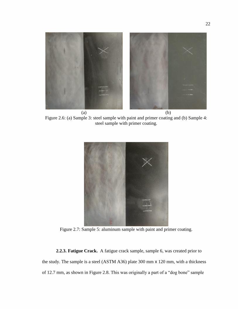
Figure 2.6: (a) Sample 3: steel sample with paint and primer coating and (b) Sample 4:

steel sample with primer coating.

Figure 2.7: Sample 5: aluminum sample with paint and primer coating.

2.2.3. Fatigue Crack. A fatigue crack sample, sample 6, was created prior to

the study. The sample is a steel (ASTM A36) plate 300 mm x 120 mm, with a thickness

of 12.7 mm, as shown in Figure 2.8. This was originally a part of a “dog bone” sample

23

that was cyclically fatigued using a closed-loop servo-hydraulic fatigue machine [28]. As

the sample was fatigued, cracks also formed around the hole shown in Figure 2.8. Unlike

the manufactured cracks, these cracks are true stress fractures, which propagated through

the entire thickness of the sample. Although this sample is a real-world crack it is

extremely narrow, and in the family of stress-induced fatigue cracks. Consequently, the

use of a higher frequency band, W-band (75-110 GHz), was required to detect this crack

at distance.

Figure 2.8: Sample 6 steel fatigue crack.

2.3. CORROSION PROCESS

The corrosion process consisted of placing each of the samples in a salt-fog

chamber for several 24-hour periods. The salt-fog chamber was a Q-FOG CCT-1100

model, which was large enough to simultaneously house all of the samples so that they

were all subjected to identical corrosion-inducing environment. The CCT-1100 also

supports a variety of ASTM standards [29]. The ASTM B117 standard was followed in

this investigation, which sets the salt concentration, temperature and humidity levels [30].

This standard seemed to work generally well for all samples since the steel samples had

24

obvious red corrosion after only 24 hours, which built up into thicker layers with longer

exposure. The samples were subjected to several 24-hour cycles of corrosion with

configuration 1 being subjected for a total of 240 hours and configuration 2 and the

fatigue crack for a total of 144 hours. After each interval was completed, the samples

were rinsed with deionized water, to remove excess salt on the surface, and were dried

over night before being imaged on the scanning tables.

25

3. IMAGING RESULTS

3.1. SAMPLE 1: SAR IMAGES AT KA-BAND (26.5 – 40 GHZ)

Sample 1 was a bare steel sample with notches as detailed by crack layout 1. A

photograph of the sample is shown in Figure 3.1(a) with the approximate scan area

superimposed on the photograph. The corresponding 0-hour SAR image, shown in Figure

3.1(b), looks as expected. The relative intensity associated with crack indications (hereon

referred to as “intensity”) in region A appear lower than the cracks in region B, which

have twice the depth. Furthermore, the relative intensity of cracks with identical width

and depth is similar, with only the smallest crack indication in region A and B being

much fainter than the rest. The relative intensity of the angled cracks also decreases as the

angle of the crack and polarization direction become parallel.

(a) (b)

Figure 3.1: (a) Sample 1 photograph prior to corrosion with marked scan area and (b)

SAR image of scan area.

26

After 24 hours, Figure 3.2 (a), and 48 hours in the salt-fog chamber, Figure 3.2

(b), most of the cracks are still detectable. Once the sample was dried, a caliper was used

to note the approximate thickness of the corrosion. Thickness measurements were taken

along the edge of the sample and averaged, the apparent change from the 0-hour

thickness was assumed to be the corrosion thickness. The corrosion rate of the steel

samples averaged ~0.125 mm per 24 hours in the salt-fog chamber but the total thickness

varies across the surface of the sample. Surface variation can be seen in the SAR images

as slight background noise, which increases in intensity as the amount of corrosion

increases. Although corrosion scatters signal at the surface, the amount of signal that is

absorbed increases as the thickness of corrosion increases, reducing the amount of signal

that reaches the crack. This effect worsens as the thickness of corrosion increases until

the crack is no longer detected, which occurs to the cracks in region A and the shortest

crack in region B, as shown in Figure 3.2 (a) and (b). Consequently, differentiating these

cracks from the background is not readily possible unless one has prior knowledge of

these crack locations.

After being in the salt-fog chamber for 72 hours, sample 1 was again

photographed. The photograph, which is shown in Figure 3.3(a), shows no visual

indications of cracks, as they are covered with a relatively significant layer of corrosion.

However, in the SAR image, Figure 3.3(b), ten of the twelve cracks are still detected. The

corrosion layer at 72 hours is almost uniform across the sample and was measured to be

~0.4 mm thick. The increase in the background clutter at this stage starts to result in false

detections, circled in white in Figure 3.3(b).

27

(a) (b)

Figure 3.2: Sample 1 SAR images after (a) 24 hours and (b) 48 hours in the salt-fog

chamber.

(a) (b)

Figure 3.3: (a) Sample 1 photograph after 72 hours in the salt-fog chamber with marked

scan area and (b) SAR image of scan area.

After having been in the salt-fog chamber for 96 hours, the highest intensity,

circled in white, is from an area of corrosion, as shown in Figure 3.4 (a). There are also a

28

few other small indications that are approximately the same intensity as the cracks that

are circled in yellow. Nevertheless, at 96 hours, 10 cracks are still detectable in the SAR

image. Although after 120 hours in the salt-fog chamber the corresponding SAR image,

shown in Figure 3.4 (b), is completely overwhelmed by the intensity of the corrosion and

no cracks are detectable. To increase the likelihood of detection the excess corrosion was

scraped off and the sample was imaged again, the resulting image is shown in Figure 3.4

(c). Removing the excess corrosion simulates an inspector preparing the surface, or

natural flaking of the corrosion off the surface, prior to the measurement. Under heavy

corrosion conditions, scraping or otherwise removing excess/loose corrosion may be

necessary. After removing the excess corrosion from the sample, as shown in Figure 3.4

(d), all 10 cracks seen in the 96-hour image, Figure 3.4 (a), are visible in the 120-hour

image, Figure 3.4 (c).

Following the removal of the excess corrosion at the 120 hours, the sample was

corroded again, for an additional 24 hours which puts the total number of hours at 144.

Eight cracks were still detected at 144 hours, as shown in Figure 3.5 (a). However,

additional corrosion inducement did not result in detecting of any of the cracks, as shown

in Figure 3.5 (b - d). As the thickness of corrosion increases, the surface of the sample

becomes irregular with areas of thicker corrosion that has built up over time. This shows

up in the SAR image as small indications that build up over time, as shown in Figure 3.5

(b-d).

29

(a) (b)

(c) (d)

Figure 3.4: Sample 1 SAR images after: (a) 96 hours and (b - c) 120 hours in the salt-fog

chamber. SAR image (b) before corrosion removal and (c) after corrosion removal.

The final cycle was completed after the sample was in the salt-fog chamber for a

total of 240 hours. A picture of the sample can be seen in Figure 3.6 (a) with the original

scan area outline. The excess corrosion on the sample was removed again similar to the

process done for the 120-hour image. The corresponding SAR image is shown in Figure

3.6 (b). While removing the excess corrosion improves the detection possibility,

30

highlighted in red in Figure 3.6 (b), the relative intensity is not much higher than the

surrounding areas making it difficult to determine if an indication is a crack, especially to

an unbiased eye. Figure 3.6 (b) further illustrates that as the amount of corrosion and

pitting increases the SAR image becomes more uniform as the magnitude of the returning

signal is equal across the entire sample.

(a) (b)

(c) (d)

Figure 3.5: Sample 1 SAR images after: (a) 144 hours, (b) 168 hours, (c) 192 hours, and

(d) 216 hours in the salt-fog chamber.

31

(a) (b)




Sample 2 is a bare aluminum sample with the notches from crack layout 1, similar

to sample 1. A photograph of the sample is shown in Figure 3.7 (a) showing the

approximate scan area. The SAR image of the bare sample, as shown in Figure 3.7 (b),

shows indications for eight of the twelve cracks, with region A cracks being undetected.

Because the cracks were made by hand, the exact depth of the cracks is not known but is

approximated. Furthermore, simulations show (in Section 4.2.2) the depth of a crack is

related to the relative intensity of the crack, with shallower cracks being less intense as

deeper cracks. Therefore, we believe it is likely that these cracks are too shallow to cause

a response in the SAR image. In Figure 3.7 (b) the cracks highlighted in red have a

distinct region where the response intensity is much stronger than the rest of the crack.

The variation along the length of the crack is thought to be due to material left over from

the cutting process (burrs). These burrs were only present on the aluminum samples,

32

which because of the material properties of aluminum, allowed the saw to tear material

away from the surface instead of the grinding process that was required to create the

cracks on the steel samples. Light sanding prior to imaging could remove these

indications but the process was not considered at the time, samples 3-5 were sanded

following the creation of the cracks.

(a) (b)



After 24 hours in the salt-fog chamber, the resulting SAR image, shown in Figure

3.8 (a), looks better than the 0-hour image. The overall quality appears improved because

the response over the length of each crack is uniform. This leads to an indication that

more closely matches a visual representation of a crack. As corrosion forms on the

surface, the effect of small physical perturbations (burrs or changes in depth) in the SAR

image are reduced. The 48-hour SAR image, which is shown in Figure 3.8 (b), looks

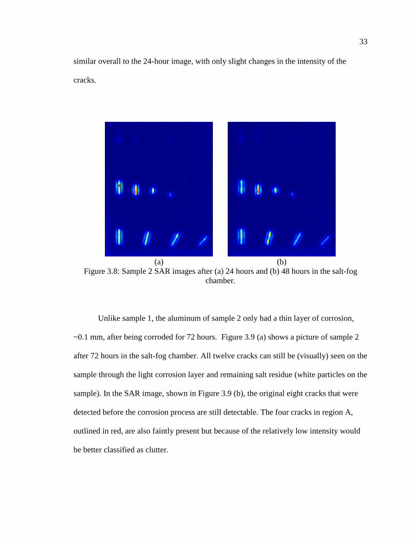
33

similar overall to the 24-hour image, with only slight changes in the intensity of the

cracks.

(a) (b)

Figure 3.8: Sample 2 SAR images after (a) 24 hours and (b) 48 hours in the salt-fog

chamber.

Unlike sample 1, the aluminum of sample 2 only had a thin layer of corrosion,

~0.1 mm, after being corroded for 72 hours. Figure 3.9 (a) shows a picture of sample 2

after 72 hours in the salt-fog chamber. All twelve cracks can still be (visually) seen on the

sample through the light corrosion layer and remaining salt residue (white particles on the

sample). In the SAR image, shown in Figure 3.9 (b), the original eight cracks that were

detected before the corrosion process are still detectable. The four cracks in region A,

outlined in red, are also faintly present but because of the relatively low intensity would

be better classified as clutter.

34

(a) (b)



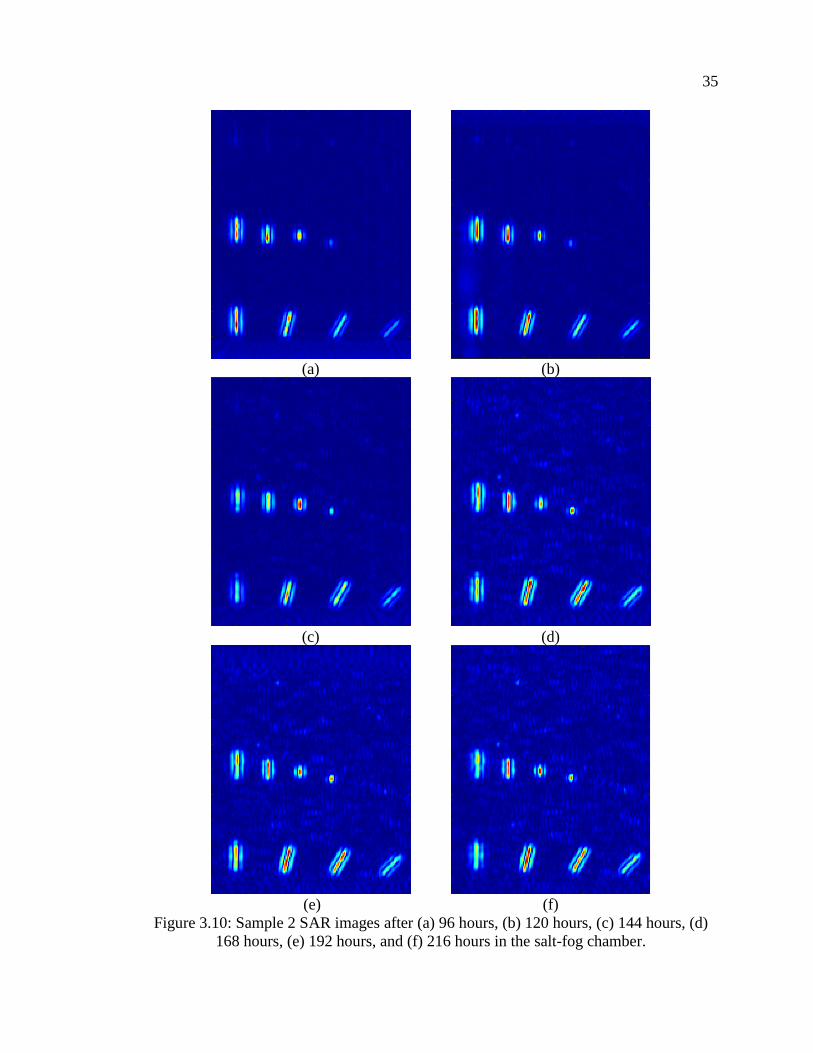
After 72 hours in the salt-fog chamber, each new 24-hour cycle did not result in

any considerable difference in the SAR images, as shown in Figures 3.10 (a-f).

Aluminum is well known for forming a thin corrosion layer that protects the underlying

metal from further corrosion [31]. The majority of the change comes from the increasing

thickness of the salt buildup from the solution inside the chamber. The increasing buildup

can be seen in the background of the SAR images after the 144 hours in the salt-fog

chamber, as shown in Figure 3.10 (c). Although the background intensity increases as the

buildup of salt increases it does not overwhelm the response from the cracks, as it did for

sample 1.

After a final 24 hours in the salt-fog chamber sample 2 was again photographed,

as shown in Figure 3.11 (a). A small amount of red corrosion can be seen on the sample

because the samples were accidently stacked before drying.

35

(a) (b)

(c) (d)

(e) (f)

Figure 3.10: Sample 2 SAR images after (a) 96 hours, (b) 120 hours, (c) 144 hours, (d)

168 hours, (e) 192 hours, and (f) 216 hours in the salt-fog chamber.

36

However, the amount of additional corrosion is very small, so the effect should be

negligible. In preparation for the final scan, sample 2 was thoroughly washed with

deionized water to remove as much of the surface salt as possible. The corresponding

SAR image with all eight cracks that were detected in the 0-hour image is shown in

Figure 3.11 (b). While the indications do not decrease in intensity with size and angle as

expected, they are still distinguishable from the background.

(a) (b)

Figure 3.11: (a) Sample 2 photograph after 240 hours in the salt-fog chamber with

marked scan area and (b) SAR image of scan area.


Sample 3 was a steel sample with the notches from crack layout 2; it has a paint

and primer coating on one-half covering two of the cracks, as shown in Figure 3.12 (a).

The 0-hour SAR image, shown in Figure 3.12 (b), shows an indication for each of the

four cracks, circled in red. The slashes that were made in the paint to facilitate corrosion

37

around the cracks are hardly visible in the SAR image because they do not scatter very

much signal. The intensity from each crack, especially those in region A, which were

through cracks, varies along the length of the crack. This is due to the large radius of

circular saw; which is only able to penetrate through the sample at the center of the crack,

while keeping the crack on the front of the sample a certain length. The change in depth

along the length of the crack causes the intensity of the crack indication to be higher in

center of the crack.

(a) (b)



After 24 hours in the salt-fog chamber, the sample was imaged again. However,

the scan step size was increased to reduce overall scan time. Increasing the distance

between sampling can also reduce the spatial resolution and can cause aliasing if the

spacing is too large [19]. These effects can be seen in Figure 3.13 (a) as the background

38

on the right, the painted side (on the right), shows some variations in image intensity that

are not present in either Figure 3.12 (b) or Figure 3.13 (b). After the 24-hour scan the

original 2 mm sampling was used throughout all the measurements as the sacrifice in

resolution did not outweigh the reduced measurement time. Unlike sample 1, which was

also steel, the first 25.4 mm long crack to become undetectable occurred after 48 hours in

the salt-fog chamber instead of after 72 hours. The cracks on the bare side of the sample

have faded into the background with only part of the crack in region A, highlighted in

red, being distinguished. However, since the background has several new indications that

could be classified as cracks the indication from region A could be misconstrued as

surface variation or otherwise.

(a) (b)

Figure 3.13: Sample 3 SAR image after (a) 24 hours and (b) 48 hours in the salt-fog

chamber.

Figure 3.14 (a) shows the SAR image after the sample was in the salt-fog

chamber for 72 hours. Neither of the bare cracks are visually detectable at this time. The

39

corrosion is quite severe that it is beginning to form at the edges of the painted half of the

sample. However, not much corrosion has penetrated the center of the protective layer

and the cracks are still visible and are detected in the SAR image, as shown Figure 3.14

(b). As the relative intensity of the corroded side of the sample increases, it begins to

overwhelm the response from the cracks. This is the reason the crack in Figure 3.14 (b),

highlighted in red, seems to disappear without additional corrosion around the crack.

Improving the contrast between the crack and the background, in this case by cropping

the corrosion out of the image, improves the likelihood that the crack will be detected

during inspection.

(a) (b)



After 72 hours in the salt-fog chamber, the corroded side of the sample started to

dominate the features in the image. Therefore, to remove this effect the corroded half was

40

removed from the following images. At 96 hours in the salt-fog chamber, the slashes that

were made on painted side are more prominent and can be seen in the SAR image, as

shown in Figure 3.15 (a). The 120-hour SAR image, shown in Figure 3.15 (b), shows

similar results, with the region A cracks having higher intensities than those in region B.

The overall background has remained mostly unchanged on the painted side, since not

much corrosion penetrated the protective layers.

(a) (b)


chamber.

After 144 hours in the salt-fog chamber the sample was photographed, as shown

in Figure 3.16 (a), and imaged, as shown in Figure 3.16 (b), for the final time. The

average corrosion thickness on the bare side of the sample was measured to be ~0.9 mm.

Furthermore, the paint and primer coating around the edge of the sample has begun to

peel off from the corrosion underneath. The slashes that were made over the cracks on the

painted side have corrosion that protrudes out further than the protective coating. While

41

the cracks on the unpainted side are no longer detectable, the cracks on the protected side

are still visible in the SAR image, as shown in Figure 3.16 (b).

(a) (b)




Sample 4 was another steel sample, similar to sample 3, however the coating on

one half was a corrosion resistant primer instead of the paint and primer mixture, as

shown in Figure 3.17 (a). Similar to samples 3 and 5, slashes were made to facilitate

corrosion around the cracks that were beneath the coating. Unlike the paint coating, the

primer coating did not flake off when scratching the surface, so each slash is made of a

few scratches to expose bare metal. In the 0-hour SAR image all four cracks were

detected, as shown in Figure 3.17 (b), as well as the border of the protective coating.

42

(a) (b)



The 24-hour and 48-hour SAR images are very similar to the sample 3 images at

the same amount of time in the salt-fog chamber. The 24-hour SAR image, shown in

Figure 3.18 (a), appears to have much more background variation, especially on the

primed half, compared to the 0-hour and 48-hour images. This variation is due to the

increase in scan step size, from 2 mm to 3 mm, between measurement points, which

causes a decrease in image quality. The scan step size was initially increased to save time

but adversely effected the SAR images. Although the additional step size reduced the

quality of the image the cracks were still detectable, and the scans were not redone.

Unlike the 48-hour SAR image of sample 3, where only three cracks were detectable

(region A crack on the bare side and both cracks on the painted side), all four cracks on

sample 4 are still detectable, as shown in Figure 3.18 (b). Slight differences, in depth and

width of the cracks, as well as the variation in the thickness of the corrosion are the most

likely reasons that all four cracks are still detectable at this time.

43

(a) (b)


chamber.

After 72 hours in the salt-fog chamber, the sample was again photographed, as

shown in Figure 3.19 (a). Corrosion not only covers the bare side of the sample but also

where the slashes were made. The corrosion at this point is almost uniform with a

measured thickness of ~0.375 mm. Figure 3.19 (b) is the last time a crack on the bare side

of the sample is detectable. The crack from region A is circled in red in Figure 3.19 (b)

based on its known location. However, because the indication is similar in intensity to

surrounding clutter the indication could easily be characterized as surface variation.

Unlike sample 3 that was coated with paint and primer, the corrosion on the primed side

was much less severe along the edges. As expected, the cracks that were coated with

corrosion resistive primer are both present, and there is little variation in the intensity of

the SAR image for primed portion. The primer layer is however very susceptible to

scratching, a small scratch from a bump with another sample is circled in red in Figure

3.19 (a). Small scratches in the protective coating lead to additional image variations that

44

could eventually mask a crack indication. However, these indications could also be used

to detect and repair the protective coating depending on the application.

(a) (b)



After 96 hours in the salt-fog chamber, the cracks on the bare side of the sample

are completely obscured by corrosion. The SAR images have been cropped to improve

the visibility of the cracks below the protective coating. Figure 3.20 (a) and (b) show the

SAR images for 96 and 120 hours in the salt-fog chamber, respectively. Both cracks are

clearly visible in both images. However, the corrosion in the slashes is more prominent

and there is additional image clutter after 120 hours in the salt-fog chamber. This clutter,

which appears as additional lines in the image, is thought to be due to an imperfect

calibration or loose connection throughout the scan as the background variation reduces

after additional time in the salt-fog chamber.

45

(a) (b)


chamber.

(a) (b)



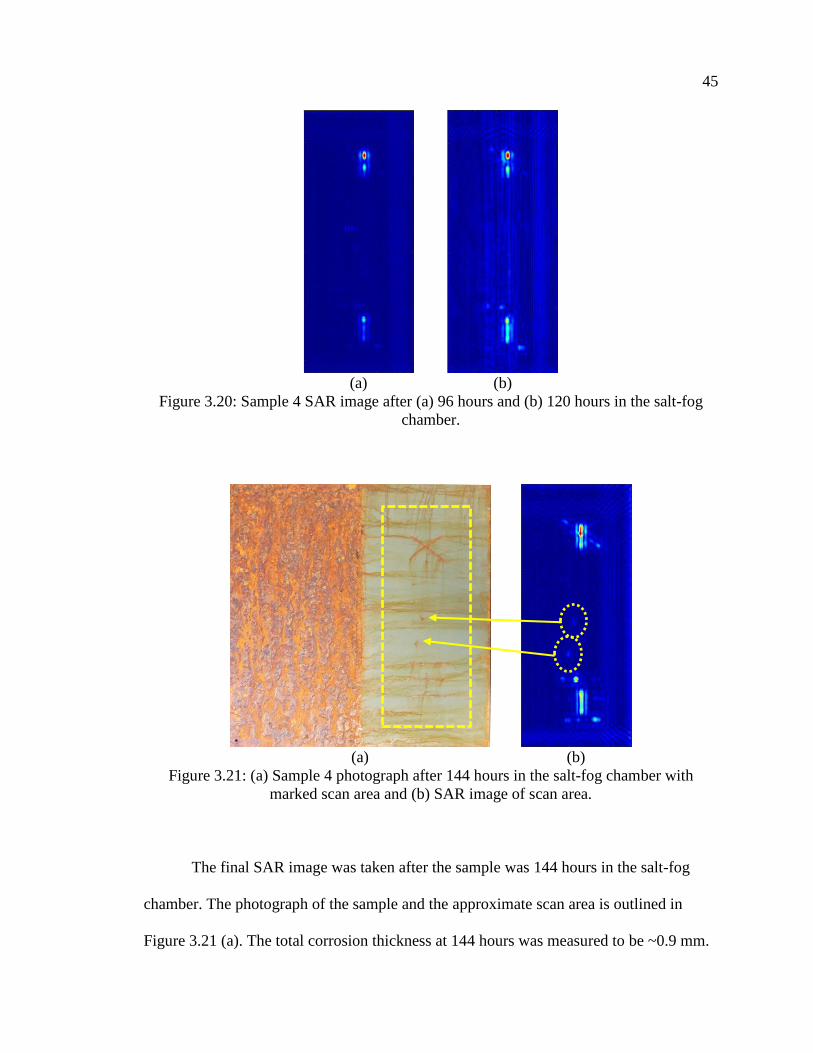
The final SAR image was taken after the sample was 144 hours in the salt-fog

chamber. The photograph of the sample and the approximate scan area is outlined in

Figure 3.21 (a). The total corrosion thickness at 144 hours was measured to be ~0.9 mm.

46

The increase in thickness is evident in the SAR image shown in Figure 3.21 (b) as the

slashes are clearly visible around the cracks. The small scratches that were accidently

made in the primer coating also begin to show more clearly in the SAR image as the

amount of corrosion from those areas exposed increases, as highlighted in Figure 3.21

(b). However, the overall background intensity is still much lower than the intensity of

the cracks, allowing for easy detection.


Figure 3.22 (a) is a photograph of sample 5, which was an aluminum sample with

notches outlined in crack layout 2 along with a paint and primer coating on one half. The

corresponding 0-hour SAR image, shown in Figure 3.22 (b), shows an indication for each

of the four cracks, highlighted in red. Similar to samples 3 and 4, the cracks in region A

appear much shorter than the actual length of the crack due to the size and shape of the

saw that was used. Although the through cracks on the aluminum sample seem to reflect

strongly, the notches that make up region B have much lower intensity and are more

difficult to distinguish.

The SAR images for hours 24 and 48 in the salt-fog chamber are shown below in

Figures 3.23 (a) and (b) respectively. Similar to previous 24-hour images, Figure 3.23 (a)

shows the reduction of image quality as the scan step size is increased, from 2 mm to 3

mm. As the intensity of the background increases, crack indications in a properly focused

image will be more easily detected. After the 24-hour image the scan step size was

returned to 2 mm for the following images. While the sample in Figure 3.23 (b) (48

hours) has undergone 24 more hours in the salt-fog chamber than Figure 3.23 (a) (24

47

hours) the intensity associated with the crack is much higher than the background

intensity and its variations.

(a) (b)



After 72 hours in the salt-fog chamber, the sample was photographed again, as

shown in Figure 3.24 (a). Similar to sample 2 the thickness of corrosion did not seem to

increase very much as a result of the additional 24 hours. At 72 hours, the total thickness

of corrosion and salt byproducts was only ~0.1 mm. If the sample was not thoroughly

rinsed, the salt layer would continue to build up as a function of increase in the exposure

time in the chamber. In real world applications, seafaring vessels may have this layer

prior to cleaning. The corresponding SAR image, shown in Figure 3.24 (b), shows a more

prominent corrosion/salt layer is more prominent and has begun to form around the

48

slashes. However, the image intensity associated with the corrosion is low compared to

the intensity of the cracks, which are all detected in the image.

(a) (b)


chamber.

After 72 hours in the salt-fog chamber, the sample was no longer cleaned after

each interval to allow the salt layer to increase in thickness to provide an example of

imaging through a non-uniform low permittivity coating. The increase in background

intensity due to the additional thickness of the salt layer can be seen in Figures 2.35 (a)

and (b). Unlike the steel samples that had little to no corrosion spread under the paint

around the slashes, sample 5 had significant bubbling of the paint around the slashes and

near the edge of the coating, examples of which are circled on Figure 3.25 (b). This

bubbling increases the variation of the background intensity around each of the cracks on

the painted side of the sample. Although aluminum oxide seems to form below the

49

corrosion resistant coating, the relative intensity of the corrosion is low enough that the

cracks may still be detectable after the coating has worn away.

(a) (b)



The final SAR image, shown in Figure 3.26 (b), was obtained after 144 hours in

the salt-fog chamber. Much like the previous cycles, all four cracks are still detected,

although the overall intensity of the background due to corrosion/salt layer has slightly

increased. The photograph of the sample at this time is shown in Figure 3.26 (a).

Additional corrosion can be seen along the edges of the paint coating and around the

slashes. The total thickness of the corrosion and salt layer was measured to be ~0.3 mm

on the bare side of the sample.

50

(a) (b)


chamber.

(a) (b)



3.6. SAMPLE 6: SAR IMAGES AT W-BAND (75 – 110 GHZ)

The final sample, sample 6, was a steel plate with two fatigue cracks. The sample

is shown in Figure 3.27 (a). A close-up image of the crack is shown in Figure 3.27 (b).

51

The corresponding SAR image is shown in 3.28. Unlike the notches that were imaged on

samples 1 – 5 this crack is extremely narrow making it much more difficult to detect.

Figure 3.28 shows an indication of a crack. However, the difference between the intensity

of the background and the crack is much lower than the 0-hour images from the other

samples. This difference normally decreases as the thickness of corrosion increases,

resulting in the crack to be undetectable much sooner than those in the other samples.

Unlike the other cracks which were created artificially the crack on sample 6 has a slight

surface level variation on each side of the crack, which makes the crack easier to detect

as the different surface levels have a higher or lower image intensity. The following

sample 6 SAR images are generated using a greyscale map instead of jet (red to blue)

colormap as the cracks were more easily seen in this presentation format.

(a)

(b)

Figure 3.27: (a) Sample 6 photograph (b) close-up of crack.

52

Figure 3.28: Sample 6 SAR image prior to corrosion.

After 24 hours in the salt-fog chamber, the sample was imaged again, as shown in

Figure 3.29. The difference in the surface level on each side of the crack is not as

prominent in this image making the indication less clear than the 0-hour image. The

corrosion has very little effect on the image, but small splotches can be seen where

corrosion is beginning to collect. In real world applications, locating the end of a crack is

pivotal as it allows an operator to inhibit progression of a crack. However, in the 24-hour

image the crack appears much shorter than it does in the 0-hour image. Although this

method cannot exactly determine the end of the crack, it can be used to determine if there

is a crack is present before surface preparation or further inspection is required.

Figure 3.29: Sample 6 SAR image after 24 hours in the salt-fog chamber.

53

The final SAR image was made after 48 hours in the salt-fog chamber. Similar to

the steel samples 1, 3, and 4, the corrosion increased after each 24 hour period in the salt-

fog chamber, with obvious corrosion after just 24 hours. This time the SAR image,

shown in Figure 3.30, shows clear signs of corrosion. Small pits and areas of higher

density corrosion are well defined, while the crack is faintly seen. Determining what is or

is not a crack at this time would heavily depend on the ability and experience of the

operator. Having the knowledge of where cracks form and how they progress will be

benficial when discriminating between corrosion, cracks and image anomalies.

Consequently fatigue cracks usually form from the edge of a material and as shown in

Figure 3.30, circled in red, a small crack can be seen coming from the center hole. The

total length of this indication has decreased after each 24-hour period in the salt-fog

chamber.

Figure 3.30: Sample 6 SAR image after 48 hours in the salt-fog chamber.

54

3.7. OVERVIEW OF RESULTS

Looking at the study as a whole we can arrive at certain conclusions. The ability

to detect surface-breaking cracks dramatically decreases as the thickness of corrosion

increases, as expected. Corrosion absorbs and scatters a millimeter wave signal. Metals

that resist corrosion or that have a corrosion resistant coating provide favorable

conditions for detecting cracks. As the corrosion builds up on the surface of a sample the

image intensity of the “background” (the portion of the image that does not have a crack)

increases. Thus, cracks are only distinguishable if there is a contrast between the crack

image intensity and the background intensity. The cracks on the bare steel samples,

samples 1, 3, and 4, were detectable up to 96 hours in the salt-fog chamber (or ~0.6 mm

of corrosion). Microscope photographs of sample 3 are shown in Figure 3.31 (a - c) as

examples of the severity of the corrosion and the condition of the sample after 144 hours

in the salt-fog chamber.

The ability to distinguish a crack from the background can be quantified by the

ratio of the mean (1) of the amplitude of the crack to the variance (2) of the

“background”; we call this quantity signal-to-noise ratio (SNR) [32]. The mean value of

the crack, 𝜇𝑐𝑟𝑎𝑐𝑘, is the summation of the pixel values (𝑠𝑖) that are in the region around

the crack, divided by the number of pixels. The squared variance of the background, 𝜎𝑏𝑔2 ,

is the summation of the difference between each pixel and the mean of the entire

“background” area, 𝑏𝑔̅̅̅̅ , squared, divided by the number of pixels minus one. Equation

(3), which shows the expression for SNR in dB is used in [32] to describe SNR in

images. Analysis using this approach was used to develop a metric associated with the

ability to detect cracks under certain conditions. The two bare samples, sample 1 and 2,

55

were analyzed to show the difference between crack indications on corrosion prone and

corrosion resistant metals. Additional analysis was performed on sample 3 to illustrate

how indications under corrosion resistant coating could be detected after much more time

in the salt-fog chamber than bare metal.

(a) (b)

(c)

Figure 3.31: Photos of (a) the bare portion of sample 3 prior to weathering, (b) the bare

portion of sample 3 after 144 hours in the salt-fog chamber, and (c) the crack and slashes

found on the painted half of region A of sample 3.

𝜇𝑐𝑟𝑎𝑐𝑘 =1

𝑁∑ 𝑠𝑖

𝑁

𝑖=1

(1)

𝜎𝑏𝑔2 =

1

𝑁 − 1∑(𝑏𝑔𝑖 − 𝑏𝑔̅̅̅̅ )

2𝑁

𝑖=1

(2)

𝑆𝑁𝑅(𝑑𝐵) = 20 ∗ log10 (𝜇𝑐𝑟𝑎𝑐𝑘

𝜎𝑏𝑔) (3)

56

The importance of analyzing the SNR associated with a crack indication in an

image is to identify how much background variation can be tolerated before a crack is no

longer detected. A threshold approach was implemented that determines if a crack is

distinguishable from the background. The value selected for this threshold (13 dB), was

determined based on the images of sample 1; 13 dB represents when the cracks were last

detectable with a minimum amount of background clutter that could be misconstrued as

cracks. This value is not absolute and should be further investigated to balance the

probability of detection and false-positives. Figure 3.32 (a) shows the SNR for the two

cracks highlighted in Figure 3.32 (b) after each 24-hour period in the salt-fog chamber.

(a) (b)

Figure 3.32: (a) SNR of the SAR indications of (b) reference for cracks 1 and 4 (region B

of sample 1) and respective noise region.

The SNR of the cracks on the steel samples constantly degraded as the amount of

corrosion increased. When the SNR dropped below the detection threshold, (i.e. there

were no crack indications) the excess corrosion was removed. This process was done at

Crack 1

Crack 4

Noise Region

57

120 and 240 hours, which is the reason for the two data points at those times. In each

case, this improved the overall quality of the SAR image. The improvement was large

enough for the 120-hour image so that the indications of the cracks were again

distinguishable from the background. However, as corrosion thickness increased, the

removal of excess corrosion did not help much in detecting the crack after additional

periods of corrosion inducing exposures. This is evident in the 240-hour image, which

showed some improvement as crack indications could be seen but were difficult to

distinguish from the background. The trend of decreasing SNR of the crack indications,

with increasing thickness of corrosion, was apparent for all the bare or partially bare steel

samples, samples 1, 3, 4, and 6.

The results of the aluminum samples, samples 2 and 5, followed a considerably

different trend. As the time in the salt-fog chamber increased, the SNR of the cracks on

the samples never fell below the detection threshold, as shown in Figure 3.33 (a). Unlike

the steel samples that continuously corroded, the aluminum samples formed a thin layer

of aluminum oxide (the corrosion byproduct of aluminum) that prohibited further

corrosion. After 72 hours in the salt-fog chamber, the sample’s surface was no longer

cleaned after each period in the chamber. As the thickness of the salt deposits increased,

the intensity of the background variation in the SAR images also increased, thus

decreasing the SNR of the cracks. Cleaning the samples prior to the 240-hour

measurement increased the overall SNR of the cracks. This may be relevant in cases of

extreme salt build up on ships or bridges that need to be inspected near saltwater bodies.

The results of the SAR images taken of the samples with corrosion resistant paints

on a portion of the sample, samples 3-5, were relatively similar to each other. The SNR

58

over time in the salt-fog chamber for two of the cracks on sample 3 is shown in Figure

3.34 (a). Cracks 1 and 2, highlighted in Figure 3.34 (b), were selected to show the

difference between a covered and uncovered crack as the thickness of corrosion

increases.

(a) (b)

Figure 3.33: (a) SNR of the SAR indications of (b) reference for cracks 1 and 4 (region B


When calculating the SNR for each crack, the noise region was selected from the

half of the sample similar to where the crack was formed. The sudden drop in SNR at 24

hours is due to the increase in scan step size (from 2 mm to 3 mm), which caused

additional background variation. This effect was removed by returning the scan step size

to 2 mm for the rest of the images. As the thickness of corrosion around crack 1

increases, the SNR of crack 1 steadily decreases until the crack is no longer detected

(below threshold), which is similar to the behavior of the SNR of the cracks on sample 1

(Figure 3.32 (a)). Crack 2, which was covered in paint and therefore protected from

Crack 1

Crack 4

Noise Region

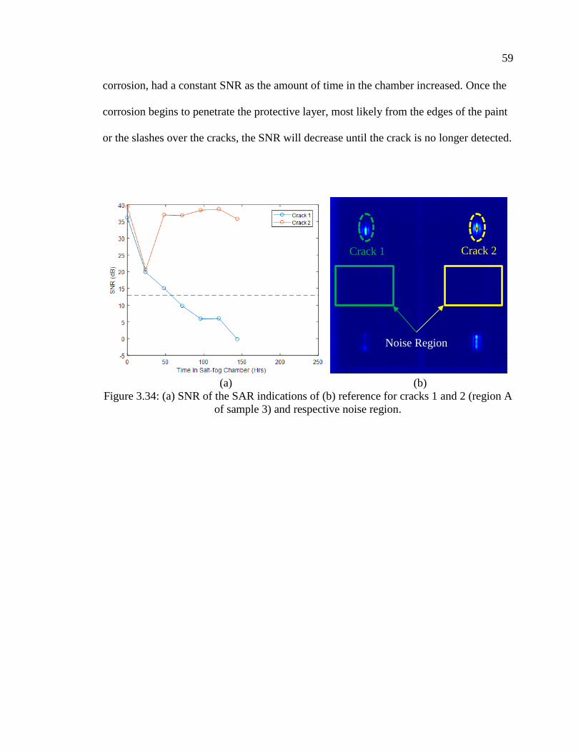
59

corrosion, had a constant SNR as the amount of time in the chamber increased. Once the

corrosion begins to penetrate the protective layer, most likely from the edges of the paint

or the slashes over the cracks, the SNR will decrease until the crack is no longer detected.

(a) (b)

Figure 3.34: (a) SNR of the SAR indications of (b) reference for cracks 1 and 2 (region A


Crack 1 Crack 2

Noise Region

60

4. NUMERICAL SIMULATIONS

In addition to the experimental measurements, numerical simulations were

performed to investigate the capability of microwave imaging to detect cracks under

surface coatings (paint, primer, and corrosion). These simulations were performed using

the EM full-wave simulation software CST Microwave Studio®. To reduce

computational time linear scans were done when investigating the effect of crack width

and depth on the SAR image across the crack. An example of the linear scanning

procedure is shown in Figure 4.1. Similar to the experimental measurements one probe

was used to measure the reflected signals from the samples. However, instead of moving

the sample around the probe, the probe was moved around the simulation domain. The

simulated images also have similar characteristics to the measurements, a step size

between measurements of 2 mm and a standoff distance of 25 mm. Additional

simulations were performed to investigate the effect of the length of a crack and the

effect of surface coatings on top of a crack. These simulations featured two-dimensional

scanning which is illustrated in Figure 4.2. All simulation data were subjected to the same

processing as the experimental measurement data.

To reduce the overall computational time, simulations were limited to a single

crack and a small imaging domain. Each simulation had an imaging domain of 30 mm x

30 mm, a step size of 2 mm and a standoff distance of 25 mm. The waveguide and the

flange had identical dimensions to those used for the experimental measurements. The

modelled crack dimensions and the surface coating of the metal were matched, as closely

as possible, to the samples. The surface coatings were simplified to their base

61

components, primer to polyamide, paint to polyurethane, and corrosion to red rust. The

dielectric constants of the paint (polyurethane εr = 3.55-j0.008) and primer (polyamide εr

= 2.6-j0.001) layers were referenced from [33]. The measured dielectric constant of red

rust, which was presented in Section 1.3.3 (εr = 8.7-j2.0) was used as well. Because the

dielectric properties of each material were not measured at Ka-band (26.5 – 40 GHz),

CST Microwave Studio® uses a built-in model to extrapolate the dielectric properties

from known frequencies, the results of this extrapolation are shown in Figure 4.3. Prior to

simulating cracks under corrosion, the effect of varying (increasing or decreasing from

the starting values) the dimensions of cracks (i.e. length, width and depth) on the SAR

image was investigated. During these analyses, the dimension being investigated was

varied while the other dimensions were held constant (if investigating the effect of length,

the width and depth were kept constant).

Figure 4.1: Top view of CST model, as a waveguide is scanned linearly across the crack

(line scan).

62

Figure 4.2: Orthographic view of CST model, as a waveguide is scanned in two

dimensions over a crack (image scan).

Figure 4.3: Dielectric constant of coatings used in numerical simulations.

4.1. CRACK RESPONSE VS. WIDTH

To investigate the effect of crack width on its SAR image a simple model of a

crack on a plate was imaged. The width of the crack was varied from 0.1 mm to 1.0 mm

and had a fixed length and depth of 25.4 mm and 1 mm, respectively. Just as the

experimental measurements were made, albeit with only one scanning direction, as

63

shown in Figure 4.1, a waveguide was moved in fixed steps across the center of the

crack. The reflected signal was measured at the waveguide as it would be if using a

network analyzer (magnitude and phase at each frequency point). The resulting linear

SAR data is shown in Figure 4.4, as the width of the crack increases the magnitude of the

indication increases. Although the manufactured cracks were all made with the same saw,

this data shows how cracks of various widths would show up in a SAR image. The

manufactured cracks also fall within the lower magnitudes as their width was between 0.1

mm and 0.25 mm. While cracks of this size are detectable, the magnitude of the SAR

image is quite low, and the effect of corrosion does not have to be that large to overpower

the crack indication. Consequently, a slightly wider crack, which has a much stronger

response, would be more easily detectable under further corrosion than the cracks used in

this study.

Figure 4.4: Magnitude of the SAR response focused at the distance of the crack as the

width of the crack varies.

64

4.2. CRACK RESPONSE VS. DEPTH

For cracks that do not penetrate through the metal surface, the depth is an

important characteristic that can limit the probability of detection. To illustrate the effect

depth has on the magnitude of the SAR image, the depth was varied from 0.25 mm to 1.5

mm, while the width and length were fixed, at 0.1 mm and 25.4 mm, respectively.

Similar to the analysis on the effect of the crack width on the SAR image, linear scans

were performed to reduce computational time while still obtaining sufficient information.

Figure 4.5 shows the magnitude of the SAR image across the width of the crack. Unlike

the crack width, there is not a direct relationship between the magnitude of the SAR data

and the depth of the crack. However, the relationship between depth and magnitude is

monotonic (increasing depth increases magnitude of SAR image). When the crack does

not fully propagate to the other side of the metal the crack acts as a cavity, making the

response a function of frequency and the dimensions of the crack, this was detailed in

[13]. As a result, the intensity of the crack indication oscillates with an overall increasing

trend as shown in Figure 4.5 [13]. The manufactured cracks in this study targeted a depth

of 0.25 mm and 0.5 mm. Cracks of around this depth appear very similar in simulation

but appeared much different in measurements, with the cracks of depth ~0.5 mm

appearing much stronger than the cracks with a depth of ~0.25 mm. This is most likely

due to the cracks being on average deeper than desired, as they were hand cut. Slight

changes in depth can have a larger impact than others, as shown in the jump in magnitude

from the depth of 1 mm to the depth of 1.25 mm, in Figure 4.5. It would have beneficial

to increase the desired depth as the response was much stronger, which could have been

detected under thicker corrosion.

65

Figure 4.5: Magnitude of the SAR response focused at the distance of the crack as the

depth of the crack varies.

4.3. CRACK RESPONSE VS. LENGTH

While changing the width and depth of a crack greatly changes the possibility of

detection, the effect of the crack length on SAR image is not as great once the crack

reaches a certain size. Similar to the other investigations, the length of the crack was

varied from 6.35 mm to 25.4 mm, while the width and depth was fixed at 0.1 mm and 1

mm, respectively. Unlike the width and depth investigations, linear scans across the crack

do not provide sufficient information to determine the effect of the length of the crack on

the SAR image. Instead, images were made, the imaging process was as shown in Figure

4.2. The resulting SAR images are shown in Figure 4.6. These images show as the length

of the crack increases the overall intensity does not increase after the crack reaches a

certain electrical length, as the 12.7 mm long crack and the 25.4 mm long crack have the

same maximum intensity. The center frequency of the band has a wavelength of ~9 mm,

which coincides with a crack length between the two shorter cracks. After this point the

66

intensity associated with the crack does not increase any longer. These simulations

closely match the measurement results of the cracks in region A of Sample 1, which are

shown in Figure 4.7. Small variations between the simulation and the measurements are

due to the slight imperfections in the manufactured cracks (i.e. different width and/or

depth between the cracks).

Figure 4.6: SAR image of simulated cracks, length from left to right: 25.4 mm, 12.7 mm,

and 6.35 mm.

Figure 4.7: SAR image of experimental cracks from sample 1 region A, length from left

to right: 25.4 mm, 19.05 mm, 12.7 mm, and 6.35 mm.

25.4 mm

12.7 mm 6.35 mm

25.4 mm

12.7 mm

6.35 mm

19.05 mm

67

4.4. CRACK RESPONSE VS. CORROSION THICKNESS

Further simulations were conducted to determine the theoretical response of a

crack with a corrosion byproduct coating. The thickness of the corrosion layer was

selected from a linear fit of the previously measured data on the bare side of sample 3, as

shown in Figure 4.8. The thicknesses were selected to be 0, 0.125, 0.25, and 0.375 mm

corresponding closely to the corrosion thickness at 0, 24, 48, and 72 hours, respectively.

The corrosion layer (red rust) was modelled on the surface of the sample; part of the

corrosion layer replaced the metal on the surface to represent metal loss. Two similar

simulation domains were created. Both included a crack with a length of 25.4 mm, a

width of 0.1 mm, and a depth of 1 mm. One had a corrosion resistant coating with a

thickness of 0.25 mm, while the other was left bare. The coating was divided into two

equal thickness of paint and primer, with the paint layer being on top of the primer layer,

the dielectric properties of both were shown in Figure 4.3.

Figure 4.8: Thickness measurements of corrosion on sample 3 over time in the salt-fog

chamber and corresponding linear fit.

68

The resulting SAR images of these two simulations are shown in Figures 4.9 and

4.10, respectively and the images are scaled to each other (similar colors represent similar

intensity). The image of the bare cracks in Figure 4.9 shows the decrease in intensity of

the crack as the thickness of corrosion increases, which is expected, as there is more loss

as the thickness increases. The image of the paint-covered cracks in Figure 4.10 shows a

similar decreasing trend in intensity as the corrosion thickness increases. However,

Figure 4.10 also shows improved focusing of the crack indication, compared to Figure

4.9, when there is an additional dielectric layer (paint and primer) above the corrosion

layer, this improvement was also shown in [34]. For these simulations, it was assumed

that the coating layer was intact, but corrosion formed between the metal layer and the

coating. While this did not happen as severely for the real samples this shows the worst-

case scenario. As expected, as the thickness of corrosion increases the amount of signal

returning from the crack decreases and the indication becomes fainter. However, these

simulations also assume that the corrosion layer is uniform in thickness and dielectric

property across the sample. In practice, corrosion is non-uniform and as such, large

changes in surface variation can mask indications of the cracks, making real world cracks

much more difficult to detect. Regardless, these simulations show that the crack

indications become much weaker under increasingly thick corrosion and will soon be

undetectable. This timeline coincides with the inability to detect cracks after the samples

had been in the salt-fog chamber for 96 hours in the experimental measurements.

69

Figure 4.9: Uncovered cracks, from left to right: 0, 0.125, 0.25, and 0.375 mm of

corrosion (Red Rust).

Figure 4.10: Cracks with a 0.25 mm thick paint and primer coating, from left to right: 0,

0.125, 0.25, and 0.375 mm of corrosion (Red Rust).

70

5. FINAL THOUGHTS

5.1. CONCLUSIONS

Detecting surface breaking cracks in metal structures under heavy corrosion is a

very difficult task. This research proposes a technique that utilizes microwave and

millimeter wave SAR imaging to detect cracks under surface coatings, such as heavy

corrosion and/or paint) and identify key characteristics of the crack such as size and

orientation. The main limitation of current techniques is the ability to detect cracks on

unclean or uneven surfaces. This study illustrated the capability of microwave SAR

imaging to detect cracks on two main types of structural metals, steel and aluminum.

Each of the six samples were placed in a salt-fog chamber for 24-hour intervals until the

cracks were no longer detected. Some of the samples were coated in a corrosion resistant

paint or primer to evaluate if the method could also be used for detecting cracks under

coatings that had been compromised by corrosion.

A standard linear-polarized, rectangular waveguide probe was used to image

samples 1 – 5 at Ka-band (26.5 – 40 GHz), and sample 6 at W-band (75 – 110 GHz). The

resulting images were visually examined for crack indications and a detection metric

(referred to as SNR), based on the relative strength of the indication compared to the

background variance of the image, was derived. This metric showed that as the thickness

of surface coating (corrosion or salt deposit) increased, the SNR of the crack indication

decreased. When the SNR of a crack indication fell below a certain threshold (defined

empirically at 13 dB, as the point where the indication could be misconstrued as

background variation) the crack was classified as undetected. This point occurred

71

between 72 and 96 hours in the salt-fog chamber for most of the cracks on the steel

samples and did not occur for the aluminum samples. Shallower cracks were the first to

go undetected, with the length of the cracks being a smaller factor of detectability (if

cracks are of sufficient length).

Numerical simulations were also conducted to verify the capability of this

method. Simulated cracks, with similar dimensions to that of the experimental samples,

were imaged at Ka-band (26.5 – 40 GHz) in a same manner as the experimental

measurements. A thin layer of corrosion was modelled on the surface, with a thickness of

approximately the measured thickness of corrosion on sample 1 after 24, 48, and 72 hours

in the salt-fog chamber, 0.125, 0.25, and 0.375 mm, respectively. The simulated images

showed that the loss from the corrosion layer makes crack indications weaker as the

thickness of corrosion increases until a point that the cracks are no longer seen. This

occurs after the corrosion thickness exceeded 0.375 mm if all parameters of the corrosion

(i.e., thickness and dielectric properties of the corrosion) are uniform throughout.

Furthermore, the simulations showed that having a thin low loss dielectric layer (in this

case paint) above the corrosion improved focusing capability, making the intensity of the

indication stronger; this was previously shown in [34].

5.2. LIMITATIONS

Although microwave and millimeter wave SAR imaging offers alternative

benefits that current methods do not provide, it does not come without its own

limitations. While microwaves can readily penetrate many materials, their interaction

with the material is significant. In this study steel corrosion, or red rust, presented the

72

biggest limitation to this method. The dielectric losses of red rust are high; the loss

tangent is about 0.25 at X-band (8.2 – 12.4 GHz), compared to that of NaCl and corrosion

resistant coatings (polyurethane or polyamide) where the loss tangent is ~0.005. This loss

was shown, in simulation and measurement, to reduce the overall intensity of crack

indications as the thickness of corrosion increases. Once the returning signal becomes too

small the crack is no longer be detectable. In the experimental measurements this point

occurred after 72 hours in the salt-fog chamber, which resulted in a corrosion thickness of

0.375 mm. The effect of this issue could be reduced if the system was optimized for

penetrating red rust corrosion, such as selecting a frequency band that has less loss

through the corrosion, or a frequency band that interacts more strongly with the crack, in

turn increasing the intensity of the crack indication. Another limitation of microwave and

millimeter wave SAR imaging is the frequency dependence on detecting small cracks. At

Ka-band (26.5 – 40 GHz) cracks with a width above 0.1 mm are detectable, albeit under

less corrosion as the intensity of the SAR image of a crack this small is very low. As the

dimensions of the crack get smaller higher frequencies are needed for detecting them.

Currently, as frequency increases hardware costs greatly increase, this could be resolved

with time as hardware prices decrease. In the end, setting a size and surface condition

threshold will be an important part of determining the limits of each system.

5.3. FUTURE WORK

While this study illustrated a capable method for detecting cracks, further analysis

may provide additional benefits of the technique. Further capability could be possible at

different frequency bands or with circularly polarized probes. Investigating different

73

frequency bands, at either, lower frequency to improve dielectric penetration (lower

losses), or higher frequency to improve crack detection capability (higher resolution and

larger interaction with crack opening), could cater microwave or millimeter wave

imaging to a specific application.

74

BIBLIOGRAPHY

[1] “Corrosion Costs and Preventative Strategies in the United States,”

https://www.nace.org/uploadedFiles/Publications/ccsupp.pdf., August 2018.

[2] “DoD Estimates the Annual Cost of Corrosion for Navy Ships,”

http://corrdefense.nace.org/corrdefense_fall_2012/DoD_1.asp. August 2018.

[3] “Highway Bridge Inspections,” https://www.transportation.gov/content/highway-

bridge-inspections. August 2018.

[4] “Nondestructive Evaluation and Structural Health Monitoring,”

https://highways.dot.gov/bridges-and-structure/long-term-bridge-

performance/nondestructive-evaluation-and-structural-health. August 2018.

[5] “Application of Magnetic Particle Inspection in the Field of the Automotive

Industry,” https://www.ndt.net/article/ecndt2006/doc/Th.1.6.3.pdf. September 2018.

[6] “The A, C and D of aircraft maintenance,”

https://www.qantasnewsroom.com.au/roo-tales/the-a-c-and-d-of-aircraft-

maintenance/., August 2018.

[7] “Aircraft Wheel and Fuselage Testing with Eddy Current and SQUID,”

https://www.ndt.net/article/ecndt98/aero/043/043.htm. August 2018.

[8] “NDT Method Summary,” https://www.nde-

ed.org/GeneralResources/MethodSummary/MethodSummary.htm., August 2018.

[9] “Eddy current imaging using array probes,”

https://www.ndt.net/events/ECNDT2014/app/content/Paper/239_Mook.pdf. August

2018.

[10] “Review of Literature on Probability of Detection for Liquid Penetrant

Nondestructive Testing,” https://pdfs.semanticscholar.org/f8a6/

ae319ec25983e7405ef092f3cc2355ae8a11.pdf, August 2018.

[11] “Review of Literature on Probability of Detection for Magnetic Particle

Nondestructive Testing,“ https://www.dst.defence.gov.au/sites/default/files/

publications/documents/DSTO-TR-2794.pdf. September 2018.

[12] Zoughi, Reza. "Microwave and Millimeter Wave Nondestructive Testing

Principles." Materials Evaluation 76.8 (2018): 1063-1069.

75

[13] Yeh, Chin-Yung, and Reza Zoughi. "A novel microwave method for detection of

long surface cracks in metals." IEEE Transactions on Instrumentation and

Measurement 43.5 (1994): 719-725.

[14] Kharkovsky, Sergey, Mohammad T. Ghasr, and Reza Zoughi. "Near-field

millimeter-wave imaging of exposed and covered fatigue cracks." IEEE

Transactions on Instrumentation and Measurement 58.7 (2009): 2367-2370.

[15] Ramzi, Mohammad R., et al. "Near-field microwave imaging using open-ended

circular waveguides." Imaging Systems and Techniques (IST), 2016 IEEE

International Conference on. IEEE, 2016.

[16] Yang, Seung-Hwan, Ki-Bok Kim, and Jin-Seob Kang. "Detection of surface crack

in film-coated metals using an open-ended coaxial line sensor and dual microwave

frequencies." NDT & E International 54 (2013): 91-95.

[17] Ghasr, Mohammad Tayeb, et al. "Comparison of near-field millimeter-wave probes

for detecting corrosion precursor pitting under paint." IEEE Transactions on

Instrumentation and Measurement 54.4 (2005): 1497-1504.

[18] Qaddoumi, Nasser N., Wael M. Saleh, and Mohamed Abou-Khousa. "Innovative

near-field microwave nondestructive testing of corroded metallic structures utilizing

open-ended rectangular waveguide probes." IEEE Transactions on Instrumentation

and Measurement 56.5 (2007): 1961-1966.

[19] Case, Joseph T., Mohammad Tayeb Ghasr, and Reza Zoughi. "Optimum two-

dimensional uniform spatial sampling for microwave SAR-based NDE imaging

systems." IEEE Transactions on Instrumentation and Measurement 60.12 (2011):

3806-3815.

[20] Ulaby, Fawwaz Tayssir, et al. Microwave radar and radiometric remote sensing.

Vol. 4. No. 5. Ann Arbor: University of Michigan Press, 2014.

[21] Ghasr, Mohammad Tayeb, et al. "Millimeter-wave differential probe for

nondestructive detection of corrosion precursor pitting." IEEE Transactions on


[22] Ghasr, Mohammad Tayeb, Kuang P. Ying, and Reza Zoughi. "SAR imaging for

inspection of metallic surfaces at millimeter wave frequencies." Instrumentation

and Measurement Technology Conference (I2MTC) Proceedings, 2014 IEEE

International. IEEE, 2014.

[23] Gallion, John R., and Reza Zoughi. "Millimeter-Wave Imaging of Surface-Breaking

Cracks in Steel With Severe Surface Corrosion." IEEE Transactions on


76

[24] N. N. Qaddoumi et al., "Microwave Corrosion Detection using Open Ended

Rectangular Waveguide Sensors," Materials Evaluation, vol. 58, no. 2, pp. 178-

184, American Society for Nondestructive Testing, Inc., Feb 2000.

[25] Bois, Karl J., et al. "Dielectric plug-loaded two-port transmission line measurement

technique for dielectric property characterization of granular and liquid materials."

IEEE Transactions on Instrumentation and Measurement 48.6 (1999): 1141-1148.

[26] Rytting, D. K. "An analysis of vector measurement accuracy enhancement

techniques." (1982).

[27] Ghasr, Mohammad Tayeb, Kuang P. Ying, and Reza Zoughi. "Wideband millimeter

wave interferrometer for high-resolution 3D SAR imaging." Instrumentation and

Measurement Technology Conference (I2MTC), 2015 IEEE International. IEEE,

2015.

[28] Qaddoumi, N., et al. "Microwave detection of stress-induced fatigue cracks in steel

and potential for crack opening determination." Journal of Research in

Nondestructive Evaluation 12.2 (2000): 87-103.

[29] “Cyclic Corrosion Testers,” https://www.q-lab.com/documents/public/6ed712e7-

2980-4634-a529-38f0def75a7a.pdf?ReturnUrl=/resources/brochures.aspx.,

September 2018.

[30] “Standard Practice for Operating Salt Spray (Fog) Apparatus,”

https://compass.astm.org/EDIT/html_annot.cgi?B117+16., September 2018.

[31] “Corrosion of Aluminum and Aluminum Alloys,”

https://www.asminternational.org/documents/10192/3456792/06787G_Sample.pdf/

c4151917-99fc-46e8-a310-d5578d0af160., October 2018.

[32] Bushberg, Jerrold T., and John M. Boone. The essential physics of medical imaging.

Lippincott Williams & Wilkins, 2011.

[33] “Dielectric Constant, Strength, & Loss Tangent,” http://www.rfcafe.com/

references/electrical/dielectric-constants-strengths.htm, September 2018.

[34] Qaddoumi, Nasser, and Reza Zoughi. "Microwave detection of corrosion under

paint and composite laminate coatings." Nondestructive Evaluation of Aging

Aircraft, Airports, and Aerospace Hardware. Vol. 2945. International Society for

Optics and Photonics, 1996.

77

VITA

John Robert Gallion was born in Saint Peters, Missouri. In May 2017, he received

his B.S. in Electrical Engineering from the Missouri University of Science and

Technology, Rolla, Missouri, USA. He assisted research endeavors at the amntl research

laboratory from November 2015 until December 2018. In May 2019, he received his

M.S. degree in Electrical Engineering from the Missouri University of Science and

Technology, Rolla, Missouri, USA. He has published several conference and journal

papers, one is listed with the references of this research. Others include research done on

material characterization and microwave and millimeter wave SAR imaging.

microwave detection of surface breaking cracks in metallic

Documents