microwave-assisted ignition for improved internal …...microwave-assisted ignition for improved...

Microwave-Assisted Ignition for Improved Internal Combustion Engine Efficiency

By

Anthony Cesar DeFilippo

A dissertation submitted in partial satisfaction of the

requirements for the degree of

Doctor of Philosophy

in

Engineering – Mechanical Engineering

in the

Graduate Division

of the

University of California, Berkeley

Committee in charge:

Professor Jyh-Yuan Chen, Chair Professor Robert Dibble

Professor Michael Lieberman

Spring 2013

1

Abstract


by


Doctor of Philosophy in Engineering - Mechanical Engineering

University of California, Berkeley

Professor Jyh-Yuan Chen, Chair

The ever-present need for reducing greenhouse gas emissions associated with transportation motivates this investigation of a novel ignition technology for internal combustion engine applications. Advanced engines can achieve higher efficiencies and reduced emissions by operating in regimes with diluted fuel-air mixtures and higher compression ratios, but the range of stable engine operation is constrained by combustion initiation and flame propagation when dilution levels are high. An advanced ignition technology that reliably extends the operating range of internal combustion engines will aid practical implementation of the next generation of high-efficiency engines. This dissertation contributes to next-generation ignition technology advancement by experimentally analyzing a prototype technology as well as developing a numerical model for the chemical processes governing microwave-assisted ignition.

The microwave-assisted spark plug under development by Imagineering, Inc. of Japan has previously been shown to expand the stable operating range of gasoline-fueled engines through plasma-assisted combustion, but the factors limiting its operation were not well characterized. The present experimental study has two main goals. The first goal is to investigate the capability of the microwave-assisted spark plug towards expanding the stable operating range of wet-ethanol-fueled engines. The stability range is investigated by examining the coefficient of variation of indicated mean effective pressure as a metric for instability, and indicated specific ethanol consumption as a metric for efficiency. The second goal is to examine the factors affecting the extent to which microwaves enhance ignition processes. The factors impacting microwave enhancement of ignition processes are individually examined, using flame development behavior as a key metric in determining microwave effectiveness.

Further development of practical combustion applications implementing microwave-assisted spark technology will benefit from predictive models which include the plasma processes governing the observed combustion enhancement. This dissertation documents the development of a chemical kinetic mechanism for the plasma-assisted combustion processes relevant to microwave-assisted spark ignition. The mechanism includes an existing mechanism for gas-phase methane oxidation, supplemented with electron impact reactions, cation and anion chemical reactions, and reactions involving vibrationally-excited and electronically-excited species. Calculations using the presently-developed numerical model explain experimentally-observed trends, highlighting the relative importance of pressure, temperature, and mixture composition in determining the effectiveness of microwave-assisted ignition enhancement.

i

Dedication

I dedicate this dissertation to my parents and my grandparents. Their selfless support of my education throughout my life, along with their encouragement, guidance, and love made me recognize the immense value of the opportunity that they have presented me and motivated me to achieve all that I have.

ii

Contents Dedication ........................................................................................................................................ i

Acknowledgements ......................................................................................................................... v

1 Introduction ............................................................................................................................. 1

1.1 Structure of the Dissertation ............................................................................................. 1

1.2 Dissertation Contributions ................................................................................................ 3

2 The need for energy-efficient technologies ............................................................................ 4

2.1 Technological developments affect energy use ............................................................... 4

2.1.1 New energy source technology ................................................................................. 4

2.1.2 Lower-cost energy source technology ...................................................................... 6

2.1.3 Cleaner technologies or those that eliminate a specific byproduct ........................... 6

2.1.4 More-efficient energy use technologies .................................................................... 7

2.2 Will energy efficiency actually reduce fuel use and harmful emissions? ........................ 8

2.3 Conclusion: Responsibly-applied energy efficiency technology is essential ................... 9

3 Plasma-Assisted Combustion State of the Art ...................................................................... 11

3.1 High-energy ignition technologies ................................................................................. 11

3.2 Experimental Evidence of Plasma-Assisted Combustion Enhancement ....................... 12

3.3 Modeling Gas-Phase Combustion .................................................................................. 13

3.4 Modeling Plasma-Assisted Combustion ........................................................................ 14

4 Engine Testing With a Microwave-Assisted Spark Plug ...................................................... 15

4.1 Introduction .................................................................................................................... 15

4.2 Experimental Approach .................................................................................................. 16

4.2.1 Engine apparatus ..................................................................................................... 16

4.2.2 Microwave-assisted ignition system ....................................................................... 17

4.2.3 Data Acquisition ..................................................................................................... 19

4.2.4 Experimental Test Matrix ....................................................................................... 19

4.3 Analysis Methods ........................................................................................................... 20

4.3.1 Calculating air-fuel ratio from exhaust gas measurement ...................................... 20

4.3.2 Calculating engine output, stability, and efficiency ................................................ 20

4.3.3 Calculating heat release rate from pressure data ..................................................... 21

4.3.4 Flame development time as a metric for early heat release .................................... 21

4.3.5 Calculating in-cylinder properties with a slider-crank code ................................... 22

iii

4.3.6 Estimating flame speed at time-of-spark ................................................................ 23

4.4 Results and Discussion ................................................................................................... 24

4.4.1 Extension of the stable operating range .................................................................. 24

4.4.2 Enhanced burning rates by microwave ignition ...................................................... 30

4.4.3 Factors influencing microwave effectiveness ......................................................... 32

4.5 Conclusions .................................................................................................................... 37

5 Plasma-Assisted Ignition Model Development .................................................................... 38

5.1 Governing Equations for Well-Mixed Reactor Model ................................................... 38

5.1.1 Electron energy equation ........................................................................................ 38

5.1.2 Electron energy source term ................................................................................... 39

5.1.3 Gas energy equation ................................................................................................ 40

5.1.4 Chemical species evolution ..................................................................................... 41

5.2 Gas-Phase combustion reactions .................................................................................... 42

5.3 Electron impact reactions ............................................................................................... 42

5.3.1 Electron energy accounting ..................................................................................... 43

5.3.2 Electron impact cross sections ................................................................................ 46

5.3.3 Calculating the rate of an electron impact process ................................................. 52

5.3.4 Combining electron impact processes with an “effective” rate .............................. 54

5.4 Modeling Excited Species .............................................................................................. 55

5.4.1 Thermodynamics of Excited Species ...................................................................... 56

5.4.2 Reactions Involving Excited Species ...................................................................... 56

5.5 Charged Species Interactions ......................................................................................... 60

5.5.1 Attachment reactions reduce the number of free electrons ..................................... 60

5.5.2 Detachment reactions release electrons from negative ions ................................... 60

5.5.3 Charge transfer reactions ........................................................................................ 61

5.5.4 Recombination reactions ......................................................................................... 61

6 Plasma-Assisted Ignition Model Results .............................................................................. 66

6.1 Introducing ignition delay calculations .......................................................................... 66

6.2 Initial electron fraction and electric field strength effects .............................................. 67

6.3 Fuel-air ratio effects ....................................................................................................... 69

6.4 Pressure Effects .............................................................................................................. 72

6.5 Discussion of pressure dependence with constant reduced electric field and reactivity 75

7 Conclusions and opportunities for further study ................................................................... 79

7.1 Engine testing summary and conclusions ...................................................................... 79

iv

7.2 Modeling summary and conclusions .............................................................................. 79

7.3 Closing thoughts ............................................................................................................. 80

8 References ............................................................................................................................. 81

9 Appendix 1: Fuel Injector Mass Flow Correlations .............................................................. 91

10 Appendix 2: Chemical Kinetic Mechanism .......................................................................... 96

11 Appendix 3: Electron impact cross sections for upper-level electronic excitation of oxygen, in BOLSIG+ format. ................................................................................................................... 152

v

Acknowledgements Though I am far from finished learning, this dissertation marks the culmination of my formal education, making this is a fitting time to recognize those contributing to my success in reaching this academic milestone. I dedicated this dissertation to my parents and my grandparents, who supported my learning throughout my life. This achievement would also not have been possible without the contributions of so many others who have shaped my experiences.

My education has been positively influenced by many exceptional individuals. All of my teachers, from preschool through graduate school, have contributed to this work by teaching me math, writing, science, art, history, foreign languages, music, and how to use a library. Mr. Barton and Mr. Brinkhorst at Burroughs put me on the path to become an engineer. Professor TenPas and Professor Burmeister at Kansas helped me find my passion in thermoscience. Mike Porter and Sean McGuffie at PMI taught me how engineering works in the real world. At Berkeley, Professor Chen always took the time to meet with me, brought enthusiasm to our all of our meetings, and was somehow always able to fix a broken computer code in a tenth of the time that it should have taken. Professor Dibble introduced me to combustion and taught me hundreds of other important things that one may never find in a textbook. Professor Fernandez-Pello also taught me a great deal about combustion processes, and I was lucky to receive his advice throughout my graduate career. Professors Lieberman and Lichtenberg wrote the book on plasma processes that taught me much of what I know about the subject. Ricky Chien taught me Linux and answered a combustion question from me every day before he graduated. Greg Bogin helped me through my first research paper and taught me how to compose a good presentation. I was lucky for several helpful discussions with Professor Fabrizio Bisetti about plasma. I am grateful to Dr. Joseph Oefelein and Dr. Guilhem Lacaze at Sandia for teaching me to use their large-eddy-simulation code. My labmates Greg Chin, Don Frederick, and Ben Wolk offered helpful comments in lab meetings, company on post-meeting trips to La Burrita, and good times at football games, camping, and exploring Poland. Extra appreciation goes to Ben Wolk for his many contributions to the engine testing section of this exploration as well as his assistance with editing parts of this manuscript. The engine testing was only possible through the efforts of Vi Rapp, Andrew Van Blarigan, Samveg Saxena, Wolfgang Hable, and others before them who built the CFR engine into the versatile research platform that it is today. Yuji Ikeda, Atsushi Nishiyama, and Ahsa Moon of Imagineering Inc. generously provided us with the prototype microwave-assisted spark system and helped us operate it on our engine.

Another thing making this dissertation possible is the various sources of funding that I have been fortunate to receive along the way, and for that I thank the University of California, the U.S. Department of Energy, the Sloan Program, the UC-Berkeley Mechanical Engineering Department, and Sandia National Laboratories. Fitting right into this section is my gratitude to MaryAnne Peters, who managed all of this for me, always with a smile and kind words. Also, Yawo, Donna, Pat, and Shareena in the M.E. office all have provided me with essential assistance in a wide range of matters through my time in Berkeley.

Outside of school, I have been lucky to have many great people helping me maintain balance in my life. My roommates through the years on Mississippi Street and at Prince ‘n King always made me feel at home despite physical distance from my family. Intramural sports, board game nights, and bike rides brought opportunities for success at times when academics weren’t progressing as well as I may have liked. I am deeply grateful to the Riera family for giving me a

vi

home in Berkeley at both the beginning and the end of my time in graduate school. Visits and phone calls with my brother Mickey are always full of laughs, and most importantly he gives me someone to brag about. Finally, I thank my very-soon-to-be-wife Caitlin for her patience, love, support, and companionship through my seemingly unending time as a student, and thank her in advance for all of those same things from this point onward.

1

1 Introduction Earth-scale temperature changes of just a few degrees Celsius over century-long timescales have motivated this investigation that has shifted to phenomena occurring at molecular length scales and nanosecond timescales, with temperature fluctuations of thousands of degrees Celsius. The critical need for reductions in greenhouse gas emissions for mitigation of global climate change prompts this journey from an overview of the need for improved energy conversion technology to a specific investigation of the basic science underlying plasma-assisted combustion technology. Energy efficiency technologies, such as the microwave-assisted spark plug analyzed in the present study, can potentially reduce the energy input needed for a given amount of usable output, serving as one of the many necessary approaches towards abating climate change. This thesis experimentally evaluates the performance of a microwave-assisted spark plug in an internal combustion engine, and then develops a numerical model for the underlying plasma-assisted combustion processes so that improved systems can be designed.

1.1 Structure of the Dissertation This thesis narrows focus from motivations at a global scale to experiments at the engine scale and then down to modeling the scales of electron-molecule interactions.

Chapter Two motivates the need for improved energy technology by identifying the major concern facing the world as not a limited supply of fuel, but instead a limited capacity of the atmosphere for absorbing carbon emissions. The general outcomes of energy technology advances are considered: (1) allowing use of a new energy source; (2) allowing lower-cost use of an existing energy source; (3) allowing cleaner use of an energy source by eliminating a specific byproduct; (4) allowing more-efficient use of an existing energy source. For each possible outcome, the potential issues necessary for consideration are deliberated, as the consequences of energy technological developments have not always been positive. The implications of improved energy efficiency are here more-deeply considered in terms of historical thought and recent literature, with the conclusion that careful application of energy efficiency technology is essential for reduction of the harmful impact of carbon dioxide emissions.

Chapter Three begins the quest towards practical application of a microwave-assisted spark plug by surveying the current state of technologies. Past high-energy ignition systems have produced faster burns and more-reliable ignition, leading to efficiency improvements by extending stable operating ranges of internal combustion engines into more-efficient regimes such as those with higher dilution (air or exhaust gas), higher turbulence, or higher compression ratios. There is room for improvement in advanced ignition device durability, cost, and efficiency, so to-date, the standard transistor-switched coil ignition systems have remained in production. Plasma-assisted combustion has shown the potential for combustion enhancement through electromagnetic interactions in weakly-ionized reacting gases, and such a technology could produce a commercially-viable ignition device.

Chapter Four analyzes the capabilities of the microwave-assisted spark plug, through analysis of a multi-parameter test matrix completed in an ethanol-fueled single-cylinder Waukesha ASTM-Cooperative Fuel Research (CFR) engine under varied conditions, notably increased compression ratio, increased preheat, and increased charge dilution. Independent variables include compression ratio (9:1, 10.5:1, and 12:1); fuel water dilution by volume (0%, 20%, 30%,

2

40%); intake air temperature (22° C, 60° C); air/fuel ratio (stoichiometric to lean-stability-limit); spark timing (advanced, maximum brake torque, retarded); and ignition strategy (spark only, spark with microwave). This section examines the extension of the stable operating range by a microwave-assisted spark plug, with data indicating that microwave-assisted spark ignition reduces cyclic variation as compared to spark-only ignition in highly-dilute mixtures at all tested compression ratios and intake air temperatures. Examination of the factors affecting microwave ignition performance shows diminished effects of microwave energy input when in-cylinder pressures are high at time of spark.

Chapter Five describes the development of a numerical model for plasma-assisted combustion with the aim of improving understanding of the processes underlying experimentally-observed ignition enhancement. A detailed chemical kinetic reaction mechanism for methane combustion with relevant plasma reactions has been assembled. A set of “cross sections” has been compiled for the elastic and inelastic collisions between electrons and the main reactants, intermediate species, and products of methane combustion. The reaction rate coefficients describing the rates of these collisional processes are then calculated using a Boltzmann Equation Solver (ZDPlasKin/BOLSIG+) for the conditions relevant to the case of study. In addition to electron impact reactions, the present mechanism includes reactions involving vibrationally- and electronically-excited species, dissociative recombination reactions, three-body recombination reactions, charge transfer reactions, and relaxation reactions, taken from the literature where available, and otherwise calculated using published correlations. The chemical kinetic mechanism is designed for use in a custom two-temperature chemical kinetics solver that tracks the electron temperature in addition to the gas temperature, as non-thermal plasma regimes characteristic to plasma-assisted combustion will typically have electron energies that are out of equilibrium with the energy of the heavier gas particle energies. The mechanism and solver will allow study of parameters relevant to microwave discharge ignition for spark-ignited engine applications.

Chapter Six delivers applies the numerical model developed in Chapter Five to problems of physical interest. Results show that depositing energy to the electrons decreases ignition delay more than if an equivalent amount of energy is deposited into the gas-phase. The effectiveness of the plasma-assisted mode is evaluated by comparing the effectiveness of energy addition compared to unenhanced ignition. The simulations predict diminished effects of electron-energy enhancement on ignition behavior as pressure is increased, consistent with experimental observation. Additional analysis considers the effects of initial temperature, mixture composition, electron concentration, and energy delivery strategy on plasma ignition effectiveness. Finally, Chemical Kinetic Sensitivity analysis under regimes of high plasma effectiveness and lower plasma effectiveness aids identification of the reaction pathways governing plasma-assisted combustion enhancement.

Chapter Seven concludes the present work by suggesting possible areas for future study and then presenting a final summary of the experiments and numerical calculations by comparing the experimentally-observed and numerically-calculated trends.

Appendix entries include: 1) Data collected for calibrating fuel injector mass injection rates to the engine control unit parameter, injector pulse width. 2) The full chemical mechanism used in the model 3) Electron impact cross sections for dissociation and excitation to high-energy electronic states of Oxygen and for dissociation of methane.

3

1.2 Dissertation Contributions This dissertation aims to advance the understanding of an advanced ignition device, the microwave-assisted spark plug, through experimental testing and numerical modeling. Some contributions to the overall body of science are as follows:

Experimental investigation of the effects of previously-untested parameters such as fuel water dilution and intake air preheat on microwave-assisted spark plug performance

Compilation of a set of reactions describing plasma-assisted combustion in methane-air and hydrogen-air mixtures

Development of a method for combining reaction rates for eliminating numerical instabilities while preserving accuracy

Evaluation of the chemical reactions important to plasma-assisted methane ignition

4

2 The need for energy-efficient technologies The well-established unsustainability of the fossil-fuel-dominated energy supply currently powering the world economy has prompted a multitude of approaches towards mitigating the scarcity of fossil resources and the environmental consequences of fossil resource extraction and use. The finite nature of fossil resources has long been known: In 1865, William Stanley Jevons predicted a peak of Britain’s coal resources, and in 1956 M. King Hubbert predicted that contiguous United States crude oil production would peak around 1970. However, improved extraction and conversion technologies have vastly increased the available resource, with Farrell and Brandt (2006) reporting that over 18,000 billion barrels of liquid hydrocarbon fuels remain in the ground, as compared to less than 1,000 billion barrels of liquid hydrocarbons so far used in the history of humanity. Unfortunately, the carbon emissions associated with extracting nonconventional fuels such are far greater than those associated with conventional oil. The problem has thus shifted from concerns with running out of fuel to a more-pressing concern of running out of space in the air for the emissions associated with fossil fuel combustion.

Increased concentrations of atmospheric carbon dioxide have intensified the greenhouse effect that maintains the earth’s temperature at habitable levels, threatening to rapidly raise terrestrial temperatures, disrupting ecosystems, melting polar ice, and increasing the frequency of extreme weather and droughts. In its most recent report, the Intergovernmental Panel on Climate Change (IPCC) has reported “unequivocal” evidence of global climate change that is “very likely due to the observed increase in anthropogenic greenhouse gas emissions.” Projected global temperature increase this century range from 1.1 °C to 6.4 °C depending on energy use scenario (IPCC, 2007.) The International Energy Agency predicts that “no more than one-third of proven reserves of fossil fuels can be consumed prior to 2050” if climate change is to be mitigated to a 2 °C temperature increase, though carbon capture and storage (CCS) technology could allow greater consumption of fossil fuels while still mitigating extreme climate change (IEA, 2012). The need to reduce fossil fuel consumption is clear. “De-growth” and the resulting overall reduction of economic activity would reduce energy use. Such an idea is politically unpopular in developed nations accustomed to a certain standard of living and to developing nations striving for modernization. New developments in energy technology can potentially advance or maintain the standard of living while reducing the harmful emissions associated with current technologies.

2.1 Technological developments affect energy use A variety of technologies being developed and deployed can aid in reduction of greenhouse gas emissions associated with energy use while maintaining or advancing the overall utility of society. Developments in energy conversion technology will typically achieve one or more of the following outcomes: 1) Allow use of a new energy source; 2) Allow lower-cost use of an existing energy source; 3) Allow cleaner use of an energy source or eliminate a specific byproduct; 4) Allow more-efficient use of an existing energy source. For all of these outcomes, specific examples of present and future technologies that achieve the outcome are presented, and the potential issues inherent to the outcome are discussed.

2.1.1 New energy source technology The first outcome of energy use technology simply allows the use of an energy source not previously available. Pre-industrial examples of energy use technology include burning of biomass, coal, and whale oil for heat and light, harnessing blowing wind or flowing water for milling grain, or putting a sail on a boat for propulsion. Since the industrial revolution, mankind

5

has developed an unprecedented demand for burning fuels derived from fossil sources (coal, oil, natural gas) and plant sugar (ethanol) for transportation, electricity, and industry. Technology has unlocked utilization of atomic energy, water potential energy, solar energy, wind energy, and the earth’s heat through respective advances in nuclear fission, hydroelectric dams, photovoltaic solar panels, wind turbines, and geothermal power plants. Future developments in energy technology will reveal additional energy sources including ocean waves, plant cellulose, high-altitude wind, and perhaps someday atomic fusion.

Many issues associated with the implementation of new energy sources deserve consideration when evaluating deployment of a new energy source, as seemingly harmless technologies will often have some shortcoming.

A first concern of energy use technology is the undesirable byproducts: As discussed previously, fuel combustion has the unfortunate side effect of releasing carbon dioxide into the atmosphere, but even “carbon-neutral” biofuels will still lead to emission of unburned hydrocarbons, oxides of nitrogen (NOx), particulates (soot). Even wind power can have the undesired byproduct of local noise and the disruption of bird flight patterns.

A second consideration is land use: biomass energy may lead to destruction of forests for cropland, hydro-electric power can flood canyons, and large solar photovoltaic arrays may disrupt the desert habitats of small animals. Land scarcity can limit the extent to which certain technologies can penetrate the market.

A third consideration of new energy technology is whether it will lead to the consumption of a finite resource either through initial production of the technology or through its use. Hunting whales for lamp oil nearly lead to species extinction. Until recent advancements in drilling technology, United States oil extraction declined as easily-accessible wells dried. Production of wind turbines, some photovoltaic solar panels, and some battery technologies may require “rare earth” metals of which supplies are limited. Growing biomass crops for fuel may require excessive water use in a world facing increasing frequency of droughts.

A fourth consideration for new energy source technology is whether existing infrastructure can sufficiently accommodate the energy source. Some biofuels, such as ethanol, cannot be pumped through the same pipelines that distribute oil and gas due to alcohol’s tendency to retain water. Additionally, the current power grid may require additional transmission lines and load-management technologies for accommodating intermittent, distributed energy sources such as solar and wind power, and offshore technologies will present even larger transmission challenges. The majority of the current fleet of land, air, and sea vehicles will not run on electricity, thus the extent to which renewable electricity generation can reduce transportation energy usage is limited.

A fifth consideration of energy technology is equity, specifically, whether production will benefit those affected by its generation and whether everyone will be able to afford the technology. The “not in my back yard” phenomenon highlights the issue of equity, where everyone wants cheap energy, but nobody wants a wind turbine whirring above their house at all hours. Equity also becomes an issue when biomass as a fuel displaces food production, raising food prices and disproportionally affecting those with the lowest incomes.

6

A sixth consideration for new energy technology is the risk of catastrophic failure during the lifetime of the technology. The most obvious example comes from nuclear power, which would represent a near-perfect technology if not for the risk of devastating meltdown as witnessed in Fukushima and Chernobyl and the lingering concerns with spent fuel disposal. Oil extraction and transport faces the risk of large spills that can harm ecosystems as seen in the case of the Exxon Valdez spill of 1989 or the Deepwater Horizon oil spill of 2010. Coal energy faces similar risks, with news stories of mine collapses and ash spills entering public conscience every few years. Additional examples of catastrophic failures from energy sources include dams breaking, wind turbines falling, or airplane fuel tanks exploding.

An seventh issue with energy technology is reliability: Grid operators can much more likely count on receiving electricity from a coal plant than a solar array, and cargo ships maintain their delivery schedules by relying on burning oil instead of intermittent wind on sails.

The eighth and final issue here considered is a main factor in determining the degree of implementation of a technology, the cost. Solar photovoltaic panels, for example, have high capital costs while natural gas, coal, and oil currently remain competitively low-cost and thus maintain their position as the leading energy sources in the world economy.

2.1.2 Lower-cost energy source technology A second outcome of energy technology development relates to the final consideration discussed in the previous section, and that is the initial cost of harnessing an energy source. Thin-film solar photovoltaics can be fabricated for a lower cost than traditional crystalline-silicon solar panels, and two-stroke engines can be built for a lower cost than four stroke engines. Thin-film panels less-efficiently convert sunlight to electricity, and two stroke engines are characterized by higher pollutant emissions and lower efficiencies. It must thus be considered whether making a lower-cost energy source technology will this lead to faster resource degradation or increased pollution. An additional consideration of lower-cost energy technology is whether it will delay or make impractical any adoption of an alternative energy technology or societal shift that could have more beneficial outcomes. Mass production of internal combustion engines coupled with low-cost fossil energy has enabled population sprawl, increasing daily driving distances. Mass transit and renewable energy sources thus have difficulty competing without subsidies or incentives. On the other hand, lowering the cost of solar and wind power presents a grand opportunity for technological advancement that will reduce environmental harm associated with energy use, as lowered costs of clean, renewable energy sources will accelerate replacement of polluting, non-renewable energy sources. If energy resources associated with current technologies were infinite and negative externalities such as pollution were negligible, then lowering the cost of all energy-use technologies would be the only remaining motivation for energy research, but given the current environmental crisis and resource scarcities facing the earth, there is also strong motivation for reducing the overall level of energy use and the associated negative byproducts.

2.1.3 Cleaner technologies or those that eliminate a specific byproduct A third important area in energy technology development is the implementation of technology that reduces specific byproducts associated with utilizing an energy source. Catalytic converters increase the cost of automobiles and prevent engine operation in certain efficient modes, but they have nevertheless been installed on most cars sold in the United States because they reduce tailpipe emissions of NOX, unburned hydrocarbons, and carbon monoxide. Carbon Capture and

7

Sequestration (CCS) technology could allow continued burning of fossil fuels for energy by pumping the carbon dioxide underground, mitigating the greenhouse effects associated with atmospheric carbon dioxide emission.

Issues for consideration with cleaner technologies include the effect on initial cost of the technology. A power plant built with carbon capture capabilities will require significantly higher capital expenditures than a traditional power plant. A clean technology can also reduce efficiency and thus accelerate resource consumption, such as in a carbon-capture scenario in which energy must go towards separating the carbon dioxide from the nitrogen in the plant exhaust before pumping exhaust underground. This will thus lead to a faster depletion of coal, gas, or oil resources. On the other hand, “clean” technology advancements can also effectively improve efficiency, given an existing set of regulations. For example, advances in exhaust gas aftertreatment that allow for capturing of oxides of nitrogen when engine exhaust has excess oxygen (lean NOx trap) will allow operation of diesel engines and “lean-burn” spark-ignited engines in more-efficient regimes that would otherwise pollute too much to see the road.

A third consideration of clean technologies is whether it is fair or acceptable to mandate that a development be utilized. With western nations having enjoyed the right to dump massive amounts of carbon into the atmosphere for centuries, it may be difficult to convince developing nations that they need to bear the cost of pumping all of their carbon dioxide underground. Without the ability to mandate worldwide adoption of carbon sequestration, implementing CCS in one location runs the risk of simply forcing relocation of economic activity (i.e. factories) to countries where electricity is cheaper because carbon dioxide emissions have not been mitigated. The successful implementation of clean technologies thus relies in a large part on actions of policy makers.

2.1.4 More-efficient energy use technologies A variety of technologies allow utilization of existing energy sources more-efficiently, meaning that the desired output can be done with a smaller input. Efficiency can be measured in miles per gallon of fuel for transportation (MPG), thermal efficiency for electricity generation from combustible sources ( , or as a fraction of energy converted in the case of solar panels or wind turbines. Examples of technologies that have improved energy efficiency throughout the years include electronic fuel injection in automobiles, improved airfoil designs on wind turbines, multi-junction solar panels, and combined-cycle operation modes of power plants. Advances in building energy, such as ventilated windows (e.g. Appelfeld and Svendsen, 2011) promise to reduce heating and cooling energy use. According to a recent report by the sustainability consulting firm, Ceres (Binz et al., 2012), energy efficiency improvements have a lower levelized cost of electricity as compared to any generation technologies currently available, and also have the lowest “composite risk,” which factors in construction costs, fuel costs, regulation risks, carbon price risks, water constraint risks, capital costs, and planning risks as compared to any currently-available generation technology.

There are several issues for consideration associated with technologies that improve energy efficiency. First of all, it is important to consider whether the energy invested in building a new system will be repaid by energy savings as compared to the existing system, for example, overall energy usage would likely increase if every driver bought a new vehicle every time the fuel economy of the latest automobile increased by one MPG. Another consideration is whether there

8

will be an unwanted byproduct associated with the efficiency technology. For example, Thomas Midgley, Jr. (1924) discovered that adding tetraethyl lead (TEL) to gasoline increases the octane number, allowing an engine to stably-run at a high compression ratio for improved efficiency (US Patent 1491998), but the neurotoxic and polluting effects of lead eventually resulted in a replacement of lead additives in fuels. Another consideration is whether rebound effects associated with efficiency technology will in fact lead to increased or continued use of a fuel instead of the desired decreases in fuel usage. With the primary motivation of this thesis the reduction of fossil fuel combustion through energy efficiency technology, the following subsection will consider the whether an energy use technology will actually decrease energy use.

2.2 Will energy efficiency actually reduce fuel use and harmful emissions? The energy efficiency technology of focus in the remainder of this thesis, the microwave-assisted spark plug (Ikeda et al., 2008) is a device that could potentially decrease fuel consumption and emissions in automotive applications. Plasma (ionized gas) is formed within the combustion chamber when microwaves are emitted as the spark plug fires. The enhanced chemical reactivity of the ionized gas may allow engine operation under more-efficient conditions, reducing emissions of nitric oxides and potentially improving fuel efficiency. Questions regarding lifecycle, health impacts, and reliability of such a system must be answered during development, but for the sake of this analysis, it will is assumed that the ultimate realization of the technology will simply reduce the fuel quantity required per mile of vehicle travel, and the consideration will focus on whether such an efficiency improvement will reduce overall fuel consumption.

An early author on energy availability, William Stanley Jevons (1906) argues in The Coal Question that although improvements in efficiency-of-use increase our “wealth and means of subsistence…in the present,” it also leads to an “earlier end” of resource availability. During Jevons’ time, improved economical use of coal allowed for its adoption into more applications and thus accelerated its use. Currently, fossil-fuel combustion has been implemented into most imaginable applications, and even with increased efficiency, current price-per-unit-energy-output has risen to a point where a simple improvement of efficiency would not likely bring fossil-fuels into applications in which they were unfeasible during the low-energy-price years of the late 1990s. Even if economic reasons do not accelerate oil consumption, the psychological aspects of using a supposedly “greener technology” could potentially lead to “rebound effects” through which people end up using more fuel than they would have otherwise used because they drive more miles or replace a smaller vehicle. Analysis of adoption patterns for hybrid vehicles, which also allow for greater output-per-unit-fuel-input, can aid forecast of the effects of a vehicle technology improvement. One analysis of Toyota Prius ownership by de Haan, Peters, and Scholz (2006) concludes that “hybrid vehicles like the Toyota Prius indeed have a [beneficial] effect on total CO2 emissions from road transport, and that rebound effects are not yet in sight.” Results of this analysis help reassure us of the potential for a positive impact of efficiency technologies, but cannot fully predict the outcome of advances.

Even if oil use is not increased by an efficiency measure, a lowered cost of using oil may delay its economical replacement by clean renewable energies and lifestyle changes. Efficiency innovations such as plasma-assisted combustion that effectively lower the cost of oil use for transportation could extend the economical use of fossil fuels, resulting in more total greenhouse gases in the atmosphere than would otherwise be emitted if “backstop” technologies such as solar-charged hydrogen fuel cells were allowed to become economically feasible. The

9

environmental consequence, increased global warming, of such a path would certainly be unwanted, but the economic pathway could be avoided if a regulated increase of oil price or a price on emissions is implemented along with efficiency improvements.

Two competing views of resource scarcity may both support efficiency improvements, but the reasons behind their support and the outcomes of policies implemented by these groups differ. Barnett and Morse (1963) argue that resource scarcity problems are unimportant and we only must worry about environmental consequences, while ecological economists concern themselves with running out of resources in addition to the social and environmental consequences of resource use. Barnett and Morse would certainly support such a use-based technological improvement, even if it led to increased current consumption of oil, as they value improved technology over resource conservation. In Scarcity and Growth, they decree, “Higher production today, if it also means more research and investment today, thus will serve the economic interest of future generations better than reservation of resources and lower current production.” Efforts towards mitigating global warming could prevent a resulting overconsumption of fossil-fuels as discussed in the previous paragraphs, but overconsumption could certainly arise if public consensus on the dangers of climate change remains slow to take hold. Ecological economists would likely endorse an efficiency improvement if it could in fact allow for a reduction of oil consumption while maintaining current welfare. Oil conservation efforts could help avoid the aforementioned negative consequences, as price decreases tied to the decrease of demand could be balanced by policy mechanisms by which price remains elevated and viability of alternate technologies (e.g. wind-generated hydrogen fuel cell hybrid vehicle) can eventually be realized.

Recent publications have identified that efficiency measures are an essential part of carbon emission abatement. Pacala and Socolow (2004) identify improvements in vehicle efficiency as one of the 14 “stabilization wedges” with the potential for reducing overall global carbon emissions by 7 GtC/year relative to business-as-usual by 2054 such that atmospheric levels can stabilize. A report in the McKinsey quarterly (Enkvist et al., 2007) identifies fuel efficiency in commercial vehicles as the measure with a large-magnitude negative cost of carbon abatement (i.e. implementing the change saves money as compared to business as-usual), second only to improved insulation in buildings.

Research towards technologies that improve efficiency such as the microwave spark plug are fundamentally worthwhile, as they can allow equivalent output from a lower input. Before rushing towards implementation of new technologies, it is crucial that society considers the possible outcomes. A lower energy-cost-per-unit-output could create economic or psychological incentives that increase oil use, accelerating resource depletion and economic harm, and efficiency measures could delay adoption of carbon-free technologies or major lifestyle changes, resulting in overall negative environmental consequences. With the potential harm of efficiency technology in mind, it is important that a balanced approach be taken when implementing a new technology. Correct safeguards that put a fair price on emissions or reserve resources for future generations, an innovation such as an optimized microwave-assisted spark plug can reduce environmental harm while improving quality of life for present and future generations.

2.3 Conclusion: Responsibly-applied energy efficiency technology is essential Energy efficiency technologies will play an essential role in reducing the harmful emissions associated with current fossil fuel consumption. As the lowest-cost and lowest-risk method of

10

carbon abatement, the feasibility of energy efficiency advances is apparent. By developing efficiency technology in advance of regulations, scientists and engineers can ensure that overall utility is maintained as policymakers enact rules that incentivize decreased energy consumption. Plasma-assisted ignition is one technological area that may improve internal combustion engine efficiency by allowing engine operation in more-efficient regimes such as at higher pressures with more-dilute fuel-air mixtures. The following chapter examines the state of plasma-assisted combustion technology, the subsequent chapter tests the ability of a microwave-assisted spark plug in an engine environment, and then following chapters will advance the development of numerical models describing plasma-assisted ignition to aid future practical implementation.

11

3 Plasma-Assisted Combustion State of the Art The literature surveyed in the current section covers the applied, the experimental, and the theoretical. First, the need for an improved high-energy ignition technology is established by discussing how high-energy ignition can improve efficiency and then surveying the strengths and weaknesses of past attempts at high-energy ignition systems. Second, a survey of experimental progress studying plasma-assisted combustion shows how such technology has enhanced combustion. Third, the various models and simplifications commonly used for traditional gas-phase combustion modeling are presented to set a context for the modeling efforts for plasma-assisted combustion modeling. Finally, a survey of the existing body of work towards modeling plasma-assisted combustion is presented, while some numerical methods are highlighted from plasma modeling outside of the combustion field, as their applicability may extend to combustion.

3.1 High-energy ignition technologies Future high-efficiency engines may require the ability to ignite a mixture under conditions where current spark ignition systems are insufficient. It has long been known that up to a certain point, dilution of the fuel-air mixture with excess air (lean-burn) or exhaust gas recirculation (EGR) increases an engine’s fuel efficiency and decreases emissions (Kuroda, et al. 1978). It is also well-documented that further dilution eventually destabilizes combustion such that cycle-to-cycle variations make engine operation impractical. Much effort has been made towards expanding these limits of stable operation over the years. This thesis examines the ability of a novel ignition technology, the microwave-assisted spark plug, in expanding operating limits in a lean-burn engine.

The enhanced fuel efficiency of engines with air or exhaust gas dilution has a multitude of sources. A dilute mixture will burn at lower temperatures, thus reducing heat losses. Mixture dilution can potentially be used for load control, reducing the pumping losses associated with throttled engine operation. Slower chemical reaction rates make diluted mixtures less susceptible to unwanted autoignition (knock), allowing engine operation at higher compression ratios (CR) than would be possible with stoichiometric mixtures. Additionally, the ratio of specific heats, / , of a lean mixture is higher than that of a stoichiometric mixture. A higher compression ratio and higher γ improve theoretical thermodynamic efficiency as in (3.1).

~ 1 (3.1)

An unfortunate characteristic of diluted charge engines is their inconsistent operation at increasingly high air-fuel ratios or EGR levels (Kuroda, 1978). Destabilization occurs because flame propagation speeds and mixture ignitability decline, leading to the onset of partial-burn and misfire (Quader, 1976). Thus, at the lean operation limit of a spark-ignited engine, advancing ignition timing will increase occurrence of misfire while retarding ignition timing will increase occurrence of partial-burn. Partial-burn occurrence can be reduced by enhancing flame propagation speed or decreasing flame travel distance. Turbulence can enhance flame speeds within the combustion chamber, but can adversely affect the ignitability of mixtures (Hill and Zhang, 1994). Fuel mixture blending with hydrogen enhances flame propagation rates in lean methane-air mixtures (Bell and Gupta, 1997), but blending hydrogen with liquid fuels such as gasoline presents its own commercial feasibility challenges. Flame-travel distance can be decreased by employing multiple spark plugs or centrally mounting the spark plug (Nakamura,

12

Baika, and Shibata, 1985). Dale et al. review high-energy ignition strategies that have been investigated for their capability to reduce burn duration and misfire (Dale, Checkel, and Smy 1997). The authors note that in most production engines, the standard transistor-switched coil spark discharge ignition (spark ignited) systems provide sufficient energy for the ignition of stoichiometric engine mixtures with moderate EGR levels. Durability, cost, and efficiency concerns of novel ignition technologies have prevented their widespread adoption. More-recently, the dual-coil offset ignition technology developed at Southwest Research Institute enabled engine operation at higher levels of EGR dilution than a traditional spark engine (Alger, 2011). The increasingly-studied field of plasma-assisted ignition and combustion presents opportunities for a new generation of ignition technology, and will be discussed in the following section.

3.2 Experimental Evidence of Plasma-Assisted Combustion Enhancement Plasma-assisted combustion research, which investigates combustion enhancement through electromagnetic interactions in gases, has the potential to bring new ignition technologies to market. It has long been known that flames contain charged particles and can be influenced by electric fields (Lawton, 1969). Fialkov (1997) provides a comprehensive review of past flame ion measurements and discusses how electric fields can affect flame propagation, flame stabilization, and soot formation. Generation or enhancement of plasma in a combustion environment through the use of microwaves (MW), radio frequency waves (RF), dielectric barrier discharges (DBD), nanosecond discharges, and other electric discharges has been shown to improve ignition characteristics and flame speeds under a variety of conditions and is thus an active area of research, reviewed by Starikovskaia, (2006) and later by Starikovskiy (2013.) Applications include high-speed scramjet combustion for aerospace applications (Shibkov et al., 2009) (Stockman et al., 2009) and automotive internal combustion engines (Ikeda 2009b) (Tanoue et al., 2010) (Pertl and Smith, 2009) (Kettner et al., 2006) (DeFilippo, 2011) (Rapp, 2012). Plasmas are commonly categorized as either “thermal” or “non-thermal.” In thermal plasmas, the electron energy is in equilibrium with the energy of the heavy particles, thus characterizing thermal plasmas with high gas temperatures and high levels of ionization. In non-thermal plasmas, energy transferred to electrons can enhance reaction kinetics without causing large increases in gas temperatures. Ombrello recently isolated the chemical effects of combustion enhancement associated with elevated concentrations of Ozone, , (2010a), from those associated with singlet Oxygen ( Δ ) (2010b). While most previous studies isolate plasma from the flame so that isolated species or effects can be studied, Sun et al., (2013) developed an apparatus for studying extinction limits of low-pressure counterflow methane diffusion flames directly interacting with a plasma, determining that a nano-second pulsed electric discharge can change the shape of the ignition-extinction curve changes shape from an S-curve to a monotonic extinction/ignition curve.

One method of delivering energy to electrons in gases that has seen considerable research attention is through microwaves. Previous research concerning microwave enhancement of hydrocarbon flame speed has offered an inconsistent range of observations and explanations for those observations, however. Groff et al. (1984) measured flame speed enhancements that they attributed primarily to local microwave heating of gases. Clements et al. (1981) also measured significant flame speed enhancement of hydrocarbon flames, but only at the lean limit and under electrical breakdown conditions, concluding that microwave enhancement of flames is impractical due to the high energy requirements. Shibkov (2009) employed freely localized and

13

surface microwave discharges for generating plasma in supersonic airflow and for igniting supersonic hydrocarbon fuel flows. Stockman et al. (2009) employed a pulsed microwave delivery strategy that reduced the energy requirement and measured up to 20% enhancement of flame speed in hydrocarbon flames, with measurements suggesting that chemical effects were likely responsible for this enhancement (Stockman, 2009). Michael (2010) and Wolk (2013) coupled spark breakdown with microwave input in quiescent fuel-air mixtures. Sasaki (2012) measured enhanced burning velocities of premixed methane-air flames in a burner subject to pulsed microwave irradiation, attributing the enhanced reactivity to energetic electron interactions since gas temperature increases were negligible.

3.3 Modeling Gas-Phase Combustion Currently, combustion processes are modeled using a number of different approaches, with simplifying assumptions often made for improved computational efficiency but preserved accuracy in modeling the phenomenon of interest. Specific areas where simplifications are often made include fluid flow, geometry, chemistry, thermodynamics, and transport properties. For example, if a combustion process is governed by fluid flow and transport, such as in a turbulent, non-premixed flame, it is likely that the model will include high-fidelity fluid flow and transport calculations but a simplified model for flame chemistry. On the other hand, a combustion process governed primarily by chemical kinetics, such as a homogenous charge compression ignition engine, may be modeled simply using two networked reactors, using a very simple model for fluid flow and heat transfer but with high-fidelity chemistry for proper prediction of ignition and pollutant formation.

In gas-phase combustion modeling, the basic set of scalars considered includes Temperature, , Pressure, , density, , and species mole fractions, , or mass fractions, . In multi-dimensional models, the velocity , , must also be considered. Additionally, sub-grid turbulence parameters such as turbulent kinetic energy and turbulent dissipation rate may be included depending on the turbulence model implemented.

Fluid flow and turbulence can be modeled many ways depending on the requirements of the calculation. The highest-fidelity models of fluid flow employ direct numerical simulation (DNS), solving the Navier-Stokes equations over a three-dimensional physical domain discretized to length scales smaller than the Kolmogorov length scale, the scale at which viscosity dissipates turbulent kinetic energy into heat (Ferziger and Peric, 2001). The high grid resolution necessary for DNS limits computationally-feasible solutions to fundamental studies. The requirement for high grid resolution can be relaxed by modeling the smaller turbulent scales with either the Reynolds Averaged Navier Stokes (RANS) (Amsden, 1997) approximation or Large Eddy Simulation (LES) (Pitsch, 2006). Typically combustion modeling thermodynamic treatment involves the ideal gas assumption, but more detailed thermodynamic models can also be used (e.g. Dahms & Oefeleien, 2013).

In many cases, lower-dimensional simulations are sufficient. One-dimensional models can calculate premixed laminar flame speeds and opposed diffusion flames structures (Kee, 1992) Turbulence can even be represented in one dimension for calculations of turbulent ignition and mixing with detailed chemistry (Kerstein, 1988). Spatially-homogeneous “Zero Dimensional” calculations are also quite useful in combustion calculations despite their lack of a spatial dimension (Lutz, 1988). Chemistry models are often validated against shock tube data using

14

ignition delay calculated with well-mixed-reactor codes e.g. (O’Conaire, 2004) (Li, 2004). Internal combustion engines can be modeled without including spatial dimensions by considering an engine as a network of two or three reactors for spark ignition engines or homogeneous charge compression ignition engines (Chin and Chen 2011).

The highest-fidelity model practically implemented for combustion chemistry includes a detailed chemical kinetic mechanism containing all of the species and reactions relevant to the fuel and oxidizer of interest, with a partial differential equation solved for the evolution of all chemical species in the mechanism. Detailed mechanisms for hydrogen combustion in air may involve only nine species and 19 reactions (O’Conaire, 2004) (Li, 2004), but mechanism size scales with increasing fuel complexity (i.e. carbon number). A recent detailed mechanism for methane oxidation includes 53 species and 325 reactions (Smith, Gri-Mech 3.0), while a recent detailed mechanism for a gasoline surrogate fuel includes 1550 species and 6000 reactions (Mehl, 2011). Simplified chemistry modeling can reduce the cost of calculations by reducing the number of chemical species considered and reducing the numerical stiffness of the mechanism. (Tham, 2008, DeFilippo, 2013). Lu (2009) reviews developments in large chemical kinetic mechanism reduction.

3.4 Modeling Plasma-Assisted Combustion Past modeling of plasma-assisted combustion has considered many of the mechanisms responsible for combustion enhancement. Konstantinovskii et al. (2005) developed a chemical mechanism for hydrogen combustion with electron enhancement. Their model showed two regimes: at low levels of electron energy enhancement, ignition delay of a homogeneous mixture was unaffected by electron energy enhancement, but at sufficiently high electron temperature, ignition delay decreased with increasing electron temperature. Bourig et al. (2009) simulated the effects of plasma-assisted combustion by assuming that enhanced electron energy goes towards electronic excitation of oxygen into singlet-delta, Δ , and singlet-sigma, ( Σ , states. Reactions involving excited oxygen have lower activation energies than those involving ground-state oxygen, thus numerical results show that elevated concentrations of excited oxygen lead to faster ignition of homogenous mixtures and higher flame speeds. Uddi (2008) coupled a Boltzmann equation solver with a set of gas-phase reactions and impact cross sections for modeling ignition in air-methane and air-ethylene. Bisetti (2012) studies electron and ion transport in methane-air flames, presenting a computationally-inexpensive method for calculating charged-species transport properties in flames.

Other modeling techniques for chemistry in non-equilibrium plasmas can be found in non-combustion fields, such as the Nitschke and Graves (1994) compare particle-in-cell modeling techniques with fluid model simulations for spatial simulations of energy transfer to electrons in low-pressure radio frequency discharges. Colella (1999) develops a finite-difference plasma fluid model with high-order spatial discretization, but chemistry was limited to electron and ion species with assumed near-Maxwellian energy distributions. More recently, Richley (2011) applied a two-dimensional axisymmetric calculation of low-pressure methane-argon-H2 plasma that included 38 chemical species, over 240 reactions, and locally calculates the electron energy distribution function throughout the spatial domain.

15

4 Engine Testing With a Microwave-Assisted Spark Plug A prototype microwave-assisted spark plug has previously been shown to extend the stability limits of gasoline (DeFilippo, 2011) and methane (Rapp, 2012) fueled engines. In the current study, the microwave-assisted spark plug is used to extend the stable operating range of an ethanol-fueled engine with fuel diluted by water and mixture diluted by air. This multiple-parameter study identifies factors contributing to the effectiveness of the microwave-assisted spark plug in enhancing engine operation.

4.1 Introduction Motivation for studying internal combustion engine operation with ethanol-water mixtures as a fuel comes from the potential for life-cycle energy savings. Ethanol, a bio-fuel compatible with an increasing number of road vehicles, is often criticized for the high energy cost of its production. Production of 100% pure, fuel-grade ethanol requires water removal through dehydration and distillation processes that demand an energy input equivalent to 37% of the energy content of the fuel (Martinez-Fries, 2007). Analysis shows that direct use of “wet-ethanol” that is 35% water by volume reduces the energy cost of dehydration and distillation to 3% of the fuel energy content (Martinez-Fries, 2007). Wet ethanol has previously been demonstrated as a fuel in Homogeneous Charge Compression Ignition (HCCI) engine operation with water dilution up to 60% water (40% ethanol) by volume (Mack, 2007).

Figure 4-1: The net energy balance for ethanol production illustrates the potential energy savings associated with using ethanol fuel that has not been dehydrated to pure alcohol. Removing all water from ethanol (left) requires expenditure of 37% of the final energy content of the fuel.

Leaving the mixture 20% water by volume (right) results in significant energy savings, increasing the net energy gain of ethanol production from 6% to 33%.

Unfortunately, ethanol fuel with water content greater than 0.5% by weight carries ions that accelerate corrosion of the fuel system (Cummings, 2011), so practical implementation of wet-ethanol as a fuel will require advances in fuel system metals or treatments. Even if corrosion issues preclude practical implementation of wet-ethanol as a transportation fuel, the present parametric study of engine performance with diluted ethanol fuel presents a fundamental dataset

16

for understanding microwave-assisted spark plug performance under a range of operating conditions.

The present experimental study has two main goals: the first goal is to investigate the capability of the microwave-assisted spark plug towards expanding the stable operating range of wet-ethanol-fueled engines. This goal is investigated by examining the coefficient of variation of indicated mean effective pressure. The second goal is to examine the factors affecting the extent to which microwaves enhance ignition processes. The factors affecting microwave enhancement of ignition processes are individually examined, using flame development behavior as a key metric in determining microwave effectiveness.

4.2 Experimental Approach The performance of the microwave-assisted spark plug technology was evaluated in a single-cylinder engine over a range of conditions to study the factors governing microwave effectiveness. The following subsections describe the engine apparatus, the ignition system, the data acquisition systems, and the methods for converting raw data into parameters of interest.

4.2.1 Engine apparatus A single-cylinder Waukesha ASTM-Cooperative Fuel Research (CFR) engine is employed in the present engine testing. A schematic of the engine system and associated sensors is presented in Figure 4-2 with engine specifications listed in Table 4-1. Intake air comes from an in-house air compressor regulated to 99±0.5 kPa and is passed through a controlled heater and an intake plenum. Intake temperatures in the present study range from 18.2 °C to 87.4 °C. Engine speed is maintained at 1200 rpm for all tests. Engine coolant temperature is controlled at 75 °C. A MoTeC M4 Engine Control Unit (ECU) controls ignition timing, fuel injection pulse width, and fuel injection duty cycle. The engine is fueled with mixtures of pure ethanol and distilled water delivered through a nitrogen-pressurized fuel system.

Table 4-1: Cooperative Fuel Research Engine Specifications

Displacement 0.616 L Stroke 114.3 mm Bore 82.804 mm

Connecting Rod 254 mm Number of Valves 2

IVO @ 0.15 mm lift -343 °CA ATDCcompression IVC @ 0.15 mm lift -153 °CA ATDCcompression EVO @ 0.15 mm lift 148 °CA ATDCcompression EVC @ 0.15 mm lift -353 °CA ATDCcompression

Engine Speed 1200 RPM Compression Ratio (CR) 9:1, 10.5:1, 12:1

17

Figure 4-2: Schematic of engine with sensor locations (dashed lines)

4.2.2 Microwave-assisted ignition system The air-fuel mixture is ignited using a prototype microwave-assisted spark plug system developed by Imagineering Inc. (Ikeda et al., 2009a), (Ikeda et al., 2009b), which couples microwave emissions to a standard spark discharge typical of current automotive engines. The ignition system can be operated with and without microwave assist. A standard spark is delivered via a discharge implementing a 1000 capacitor and an automotive ignition coil, initiating plasma in the combustion chamber through DC breakdown across a NGK BP6ES spark plug. Along with the spark, 2.45 GHz microwaves generated by a magnetron from a commercially-available microwave oven are directed through the spark plug insulator and into the combustion chamber. The microwaves transfer energy to the free electrons generated in the initial spark plasma and flame kernel. A schematic of the ignition system is shown in Figure 4-3.

18

Figure 4-3: Schematic of microwave-assisted spark system provided by Imagineering, Inc.

Pulsed power input to the magnetron has a peak power of 2.6 kW with about 500W average power. Power is pulsed to the magnetron at a 25% duty cycle: “on” for 4 μs followed by 12 μs “off.” The total microwave energy input can be varied by modifying the total duration of the energy input pulse train, but the amplitude of energy input is not presently adjustable. For the current tests, the microwave input duration is set to 2.5 ms per spark event. Because of microwave reflection, transmission losses, and magnetron inefficiencies, the microwave power delivered to the spark zone is about 20% of the power consumed by the magnetron (i.e. 80% loss). Reflected microwaves are measured using a 50 dB directional coupler. The microwave is started 0.25 ms before spark initiation, with a total duration of 2.5 ms, corresponding to a microwave energy input to the combustion chamber after spark initiation of about 220 mJ. The microwave spark system is tuned to minimize measured reflected microwaves, but the combustion chamber is not optimized towards promoting constructive interference of microwaves.

Figure 4-4: Timing diagram for triggering of the spark event and microwave power supply

The microwave-assisted spark plug under development by Imagineering Inc. initiates plasma using a standard spark discharge from an ignition coil, then enhances electron energy and expands the plasma by emitting microwaves into the combustion chamber. Microwaves

19

generated by a magnetron at a frequency of 2.45 GHz are transmitted through the spark plug insulator into the combustion chamber. In the combustion chamber, microwaves are absorbed by the free electrons in the spark discharge, generating non-thermal plasma. The Imagineering Inc. microwave-assisted spark plug cannot generate plasma without first initiating a spark discharge, indicating that microwaves do not create plasma simply by a coronal discharge between the conducting spark plug electrode and the ground (Ikeda, 2009a). Electric field simulations by the designers of the microwave spark plug system in a 75 mm diameter x 130mm cylindrical chamber estimate the maximum electric field strength, concentrated at the electrode, as approximately 2000 V/m, with field strength attenuating approximately by the third power of distance from the spark plug electrode (Ikeda, 2009c), a decay rate perhaps relating to the exponential Bouger law decay of an electromagnetic wave propagating into a plasma (Fridman, 2011.) The rapid attenuation of microwave power with distance from the electrode implies that as the flame front grows away from the electrode, there is little microwave energy remaining which can be coupled into the flame front. The benefits of the microwave assist are thus only realized in the early stages of combustion when the flame kernel is still near the spark electrode. The designers of the microwave-assisted spark system spectroscopically measured high levels of OH radicals during the microwave discharge event, concluding that electron-impact reactions with water molecules in the microwave plasma increase the pool of oxidizing radicals, enhancing the early stages of combustion through chemical effects (Ikeda, 2009a).

4.2.3 Data Acquisition Engine performance is evaluated on the basis of in-cylinder pressure and exhaust gas measurements. Cylinder pressure is measured using a 6052B Kistler piezoelectric pressure transducer, with signals amplified by a 5044A Kistler charge amplifier. The cylinder pressure transducer is mounted in an extra spark plug hole in the cylinder head. For each operating condition, 200 cycles of in-cylinder pressure data are recorded, with data measured every 0.1 crank angle degree (°CA). Intake pressure is measured using a 4045A5 Kistler piezoresistive pressure transducer, with signals amplified by a 4643 Kistler amplifier module. Crank angle position is determined using an optical encoder, while an electric motor controlled by an ABB variable speed frequency drive controls the engine speed.

Exhaust gas composition is measured for determination of air-fuel ratio and pollutant production. Exhaust gas is sampled downstream of the exhaust port as sketched in Figure 4-2. Water is condensed from the sample line, and the sample is sent to a Horiba gas analyzer. The gas analyzer measures concentrations of unburned hydrocarbons, oxygen, carbon monoxide, carbon dioxide, and nitric oxides (NOx). Each gas analyzer is calibrated with a “zero gas” (nitrogen) and a “span gas” of known concentration.

4.2.4 Experimental Test Matrix The experimental test matrix is summarized in Table 4-2 below. Tests were run at three values of compression ratio (CR): 9:1, 10.5:1, and 12:1; four mixtures of ethanol and water: 100%, 80%, 70%, and 60% ethanol by volume; two target intake temperatures (Tintake): 22 °C and 60 °C; a range of air-fuel mixtures from near stoichiometric to lean stability limit; and two ignition modes: microwave-assisted spark and spark-ignited only. Additionally, spark timing was varied to find maximum-brake-torque conditions and for investigation of microwave effects with advanced and retarded timing.

20

Table 4-2 - Experimental Conditions

Compression

Ratio

Fuel mix

by volume

Tintake

Air-fuel ratio

(λ)

Ignition Mode Spark Timing

100% Ethanol

22 °C

Stoichiometric Spark-Ignited

Only

Advanced

9:1

↓

↓

Maximum

Brake Torque

↓

80%

Ethanol

10.5:1

70%

Ethanol

60 °C Microwave-

Assisted Spark

12:1

60% Ethanol

Lean Retarded

4.3 Analysis Methods Raw measurements of intake pressure, in-cylinder pressure, intake temperature, and exhaust gas concentration must be converted to more-useful parameters for an in-depth analysis of the combustion processes of interest. The following subsections discuss the methods for calculating the engine parameters of interest.

4.3.1 Calculating air-fuel ratio from exhaust gas measurement For a fuel of general formula , here ethanol, , the normalized air-fuel ratio, , is estimated by assuming complete combustion and using the measured exhaust gas concentrations of oxygen, [O2], and carbon dioxide, [CO2], as in Equation (4.1).

1–

1 (4.1)

Air-fuel ratio calculated from exhaust gas measurements using equation (4.1) correlates with the amount of pure ethanol injected divided by the normalized mass of air inhaled, inferred from measurements of intake manifold temperature and pressure. For each ethanol-water mixture, a correlation was developed so that air-fuel ratio could be determined even when exhaust gas measurements were unreliable due to instabilities and incomplete burning.

4.3.2 Calculating engine output, stability, and efficiency Engine output is determined using indicated mean effective pressure (IMEP). IMEP is calculated from the recorded pressure trace for each of 200 consecutive cycles using equation (4.2). Gross IMEP includes work during the compression and power strokes (Heywood, 1988).

21

∮ ∙ (4.2)

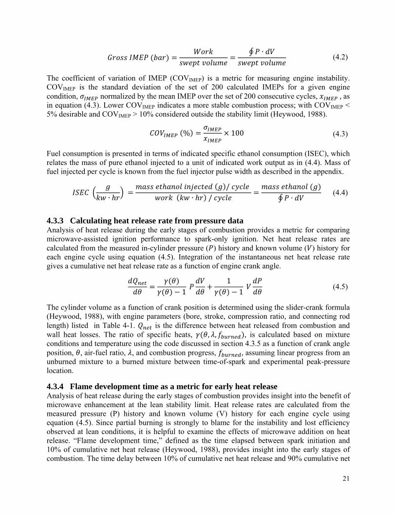
The coefficient of variation of IMEP (COVIMEP) is a metric for measuring engine instability. COVIMEP is the standard deviation of the set of 200 calculated IMEPs for a given engine condition, normalized by the mean IMEP over the set of 200 consecutive cycles, , as in equation (4.3). Lower COVIMEP indicates a more stable combustion process; with COVIMEP < 5% desirable and COVIMEP > 10% considered outside the stability limit (Heywood, 1988).

% 100 (4.3)

Fuel consumption is presented in terms of indicated specific ethanol consumption (ISEC), which relates the mass of pure ethanol injected to a unit of indicated work output as in (4.4). Mass of fuel injected per cycle is known from the fuel injector pulse width as described in the appendix.

∙

/∙ /

∮ ∙ (4.4)

4.3.3 Calculating heat release rate from pressure data Analysis of heat release during the early stages of combustion provides a metric for comparing microwave-assisted ignition performance to spark-only ignition. Net heat release rates are calculated from the measured in-cylinder pressure ( ) history and known volume ( ) history for each engine cycle using equation (4.5). Integration of the instantaneous net heat release rate gives a cumulative net heat release rate as a function of engine crank angle.

1

11

(4.5)

The cylinder volume as a function of crank position is determined using the slider-crank formula (Heywood, 1988), with engine parameters (bore, stroke, compression ratio, and connecting rod length) listed in Table 4-1. is the difference between heat released from combustion and wall heat losses. The ratio of specific heats, , , , is calculated based on mixture conditions and temperature using the code discussed in section 4.3.5 as a function of crank angle position, , air-fuel ratio, , and combustion progress, , assuming linear progress from an unburned mixture to a burned mixture between time-of-spark and experimental peak-pressure location.

4.3.4 Flame development time as a metric for early heat release Analysis of heat release during the early stages of combustion provides insight into the benefit of microwave enhancement at the lean stability limit. Heat release rates are calculated from the measured pressure (P) history and known volume (V) history for each engine cycle using equation (4.5). Since partial burning is strongly to blame for the instability and lost efficiency observed at lean conditions, it is helpful to examine the effects of microwave addition on heat release. “Flame development time,” defined as the time elapsed between spark initiation and 10% of cumulative net heat release (Heywood, 1988), provides insight into the early stages of combustion. The time delay between 10% of cumulative net heat release and 90% cumulative net

22

heat release is here called the “flame rise time.” Figure 4-5 shows the flame development time and flame rise time on a plot of cumulative net heat release calculated from engine pressure data for a single cycle.

Figure 4-5: Cumulative net heat release calculated for a single engine cycle from pressure data collected at 1200 RPM. The “Flame Development Time” is the time from spark initiation to 10% of cumulative net heat release. The “Flame Rise Time” is the time from 10% to 90% cumulative

net heat release. The microwave input duration of 18 °CA is shown for illustration.

4.3.5 Calculating in-cylinder properties with a slider-crank code An implementation of the slider-crank formula (Heywood, 1988) in Cantera (Goodwin, 2003) simulates mixture evolution inside a compressing piston by integrating the energy conservation equation for a gas mixture subject to a crank-angle-dependent volume, allowing estimation of not-easily-measured parameters such as in-cylinder temperature and specific heat ratio as a function of crank angle and the experimental conditions which serve as the initial conditions for the model.

The energy equation takes the form of a differential equation for in-cylinder temperature, , as in

(4.6). The first term accounts for compression work, ∙ ~ . The second term accounts for net

species internal energy change from chemical reactions, with ~∙

the net formation rate of

chemical species , ~ the internal energy of species at temperature , and ~

the in-cylinder volume at time . The third term accounts for wall heat losses, , ~

, ∙ ∙ , modeled using the Woschni (1967) model, with ~ the

cylinder wall area, and , ~∙, the instantaneous heat transfer coefficient, proportional to

−40 −20 0 20 40 60 80 1000

500

1000

1500

°CA ATDC

Cum

ulat

ive

Net

Hea

t Rel

ease

d (J

)

MicrowaveDuration, 18°

FlameDevelopment

Time

Spa

rk 10% of total net heat release

100% of total net heat release

90% of total net heat release

FlameRise Time

23

. ∙ . and a constant factor tuned for agreement between predicted and experimental pressure history of motored engine cycles at the various compression ratios and intake air temperatures employed in the present study. The denominator of the energy equation includes the mixture density ~ / , the cylinder volume ~ , and the average mixture heat

capacity, ~∙

. At each time step of the calculation, Cantera calculates the specific heat ratio

of the unburned mixture, / .

T ∙ ∙ ∑ ,

∙ ∙

(4.6)

Once the simulated piston reaches top-dead-center (TDC), the unburned temperature at TDC, which has increased from the initial temperature due to compression heating, is recorded as the “unburned temperature at top-dead-center,” as well as the unburned gas specific heat ratio,

. A chemical equilibrium calculation beginning with the gas mixture in its TDC condition, holding enthalpy and pressure constant, finds the constant-pressure adiabatic flame temperature, referenced as the “burned temperature at top-dead-center,” as well as the burned gas specific heat ratio, . The unburned and burned TDC temperatures define the regime diagram as will be discussed in Section 4.4.1 for consistency with the procedure of generating a regime diagram by Lavoie (2010).

4.3.6 Estimating flame speed at time-of-spark For estimating trends in flame speed at time-of spark, the laminar flame speed correlations provided by Bayraktar (2005) are applied using the measured in-cylinder pressure at time of spark, ,calculated in-cylinder temperature at time of spark, , and the normalized fuel-air ratio, as in (4.7). The correlation is for pure ethanol only, and in-cylinder turbulence is unknown, so trends in flame speed are here only suitable for comparing trends a fuel mixture with those of that same fuel mixture.

S , , 46.50 ∙ . ∙ e . ∙ . ∙

300

. 1

. /

(4.7)

Inverse flame speed, is the inverse of the flame speed calculated in equation (4.7), and

is used as an estimated factor for correlating in-cylinder conditions with time that the flame kernel is near the spark plug. There is good correlation between the inverse flame speed of a pure ethanol mixture calculated using time-of-spark temperature and pressure and the spark-ignited flame development time (SIFDT) for various ethanol-water mixtures as shown in Figure 4-6.

24

Figure 4-6: Inverse flame speed calculated for a pure ethanol fuel from conditions at time-of-spark ( , , correlates with the spark-ignited flame development time for each fuel mixture.

4.4 Results and Discussion The following subsections present an analysis of the large amount of experimental data collected and diagrammed in Table 4-2 with a narrowing focus. First, the practical considerations of the microwave-assisted spark are considered: analysis focuses on the extent to which microwave-assist expands the stable operating range of a wet-ethanol-fueled engine as compared to standard spark ignition operation. Next, the focus narrows to an analysis of burn characteristics, with data showing that microwave assist enhances early heat release rates under certain conditions of engine operation. Finally, the factors contributing to microwave effectiveness are explored through isolation of specific variables and analysis of their impact on microwave effectiveness.

4.4.1 Extension of the stable operating range A main goal of this study is to investigate the possibility of extending the stable operating range of a spark-ignited engine with wet-ethanol as a fuel. The fuel compositions, air-fuel mixtures, and intake temperatures span a wide range of operating modes. The multi-mode combustion diagram of Lavoie et al., which delineates the possible regimes of internal combustion engine operation, is a useful tool for visualizing a large range of engine modes (Lavoie et al., 2010). Operating points of the multi-mode combustion diagram are described by the unburned and burned gas temperatures at top-dead-center. The unburned and burned gas temperatures for a given operating point depend on the compression ratio, the fuel mixture, the intake air temperature, and the air-fuel ratio. With operating conditions defining initial conditions and engine geometry, the procedure discussed in section 4.3.2 solves for unburned and burned gas temperatures for each experimental condition. Conditions with higher intake temperatures and

0 1 2 3 4 50

5

10

SI

FD

T (

ms)

SL,E100−1 (ms/cm)

100% Ethanol

0 1 2 3 40

2

4

6

8

SI

FD

T (

ms)

80% Ethanol

0 0.5 1 1.5 20

2

4

6

8

SI

FD

T (

ms)

70% Ethanol

0 0.5 1 1.50

2

4

6

8

SI

FD

T (

ms)

60% Ethanol

SL,E100−1 (ms/cm)

SL,E100−1 (ms/cm) SL,E100

−1 (ms/cm)

25

higher compression ratios will have higher unburned temperatures at TDC. Conditions with high charge dilution, whether by water-fuel mixing or air dilution (lean-burn) have lower burned temperatures at TDC due to increased mixture heat capacity relative to the amount of fuel injected, and thus a reduced adiabatic flame temperature.

All experimentally-measured stable engine operating points (COVIMEP < 10%) are plotted on the regime diagram in Figure 4-7 for both ignition modes: spark-only and microwave-assisted ignition. The operating points exhibiting stable operation are connected in planes, with the plane for microwave-assisted spark operation extending into regions with lower “burned” temperatures than the plane of the spark-ignited-only mode. This indicates that the microwave-assisted spark mode allows stable engine operation in mixtures with higher dilution and corresponding lower flame temperature. Stability limit extension by microwave-assisted spark occurs over all “unburned” temperatures, indicating that the microwave-assisted spark effectively extends stability limits even with high intake temperatures and high compression ratios. Microwave extension of the stability limit diminishes at the highest unburned gas temperatures.

Figure 4-7: Regime diagram of engine operation showing that microwave-assisted spark allows stable engine operation (COVIMEP < 10%) in a larger range than possible with spark ignition

only. Microwave assist extends stable engine operation into regimes with lower flame temperatures (increased charge dilution).

4.4.1.1 Extension of stability range with air dilution and water dilution Though the regime diagram concisely demonstrates an overall extension of the stable operating range by the microwave-assisted spark mode, it does not indicate whether the instabilities overcome by the microwave-assisted mode are due to charge dilution with air or fuel dilution with water. The remainder of this section presents examples suggesting that the microwave-assisted spark plug is effective in counteracting instability caused by both air dilution and water dilution.

520 530 540 550 560 570

1400

1500

1600

1700

1800

1900

2000

2100

2200

2300

2400

TDC Temperature Unburned [K]

TD

C T

empe

ratu

re B

urne

d [K

]

Stable range of microwave-assisted ignitionStable range of spark-only ignition

Knock Limit

Stability Limit of Spark-Only Ignition

Stability Limit of Spark + MW

Increasing Compression Ratio

Increasing Intake Temperature

Incr

easi

ng M

ixtu

re D

ilutio

n

26

At a given engine condition (fixed CR, Tintake, fuel type, and engine speed), reducing the mass of fuel injected per cycle from stoichiometric conditions increases the air-fuel ratio (lean), eventually leading to engine instability as indicated by a high COVIMEP. Figure 4-8 shows destabilization of lean engine operation in terms of COVIMEP vs. at compression ratio = 9:1 and intake temperature = 60°C, with 100% ethanol fuel (W0) and 80% ethanol/20% water (W20) by volume fuel. For both fuel types, the engine is stable at nearer-stoichiometric conditions, λ < 1.5, and the microwave-assisted ignition mode does not improve engine stability. As the air-fuel ratio increases, engine operation destabilizes, with COVIMEP of the spark-only ignition mode increasing outside of the stable range. Both fuel mixtures destabilize, but the greater water dilution of the W20 case causes destabilization at a lower air-fuel ratio. Addition of microwave energy to the ignition event reduces COVIMEP at high air-fuel ratios, improving stability.

Figure 4-8: Microwave-assisted ignition (red, solid lines) reduces COVIMEP once dilution has destabilized spark-only operation (blue, dashed lines). Microwave assist does not affect stability

at closer-to-stoichiometric conditions. 1200 RPM; CR = 9:1; Tintake = 60 °C; 100% ethanol (circles) and 80% ethanol, 20% water (squares) by volume fuel mixture with water.

In addition to improving stability when engine operation has been destabilized by air dilution, the microwave-assisted spark ignition mode can improve stability when engine operation is destabilized by water dilution of the fuel. The engine was run with a constant amount of pure ethanol injected per cycle, with varied amounts of water dilution mixed with the fixed amount of ethanol. Comparison of engine data with a fixed mass of ethanol injected per engine cycle (0.042 g) and varied amounts of water dilution in Figure 4-9 and Figure 4-10 show that water dilution can destabilize engine output, increasing COVIMEP to unacceptable levels. Water dilution decreases engine output if instabilities limit complete burning. Reduced output is attributable to the unstable operation and the higher mixture heat capacity. Microwave-assisted ignition

1 1.2 1.4 1.6 1.8 20

5

10

15

20

25

30

35

40

45

Normalized Air/Fuel Ratio [λ]

CO

VIM

EP [

%]

Compression Ratio = 9:1 80% EtOH20% H2OSpark+MW

80% EtOH20% H2OSpark Only

100% EtOHSpark+MW

100% EtOHSpark Only

27

improves stability, resulting in increased average power input as compared to unstable operation in the spark-only ignition mode.

Figure 4-9: For a fixed air-fuel ratio near the lean stability limit, increasing fuel water dilution can destabilize engine operation. Microwave-assisted ignition improves engine stability slightly as compared to spark-only ignition when total dilution has destabilized engine operation. 1200

RPM; CR=9:1; Tintake = 60 °C; λ 1.65 0.025. Engine instability prevented data collection in spark-only mode with 40% water.

Figure 4-10: Under stable conditions with a fixed air-fuel ratio, 1200 RPM; CR=10.5:1; Tintake = 25 °C; λ 1.2 0.01, increasing water dilution of fuel can reduce indicated output (IMEP,

left). The reduced output at higher dilution levels under stable conditions can be partially attributed to the lower specific heat ratio of the water-diluted mixture. Microwave-assisted does

not significantly affect engine stability at already-stable conditions (COVIMEP, right).

4.4.1.2 Effect of microwave input on engine efficiency Since the main motivation for the present undertaking is the improvement of energy efficiency, it is important to examine the effect of stability limit extension on efficiency. Figure 4-11 plots

0 20 300

10

20

30

40

50

Fuel Water Vol. Fraction [%]

CO

VIM

EP [

%]

CR = 9:1, λ = 1.65±0.025

0 20 303.5

4

4.5

5

5.5

6


IME

P [b

ar] SI SI

SI + MW

SI + MW

0 20 30 401

2

3

4

5

6


CO

VIM

EP [

%]

CR = 10.5:1, λ = 1.2±0.01

0 20 30 408.4

8.6

8.8

9

9.2

9.4


IME

P [b

ar]

SI SI+MW

SI

SI+MW

28

indicated specific ethanol consumption, an inverse measure of efficiency, against engine output for a range of fuel mixtures and air-fuel ratios. Engine output decreases from full load by decreasing the mass of fuel injected per cycle such that the engine enters lean-burn mode. At slightly lean conditions, efficiency improves. As air-fuel ratio increases and the engine destabilizes, efficiency drops as an increased frequency of partially-burning cycles leaves some fuel unburned. Microwave enhancement mitigates the instability at low-load conditions, reducing the efficiency fall-off of by reducing the frequency and severity of partial burn cycles. The extension of stability limits by microwave-enhanced ignition allows efficient operation over an extended lean-burn range as compared to spark-only ignition. However, the greatest overall efficiency is not achieved due to lean-limit extension, as the improvements of stability by microwaves at lean-burn conditions do not fully eliminate the occurrence of partial-burn cycles.

Figure 4-11: Fuel consumption per unit output plotted against engine output for a range of fuel mixtures at Compression Ratio of 10.5:1, wide-open-throttle, intake temperature = 22 °C. Engine output is decreased from full load by decreasing the mass of fuel injected per cycle. At slightly reduced load (slightly lean), efficiency improves. As air-fuel ratio further increases, the load

decreases and the engine destabilizes. The extension of stability limits by microwave-enhanced ignition (triangles) allows efficient operation over an extended lean-burn range as compared to

spark-only ignition (circles). Injector output limited high-load operation with 40% ethanol.

5 6 7 8 9 10

400

420

440

460

480

500

520

Indicated Mean Effective Pressure [bar]

Indi

cate

d S

peci

fic

Eth

anol

Con

sum

ptio

n [g

/kW−

hr]

CR = 10.5:1

100% Ethanol0% Water

80% Ethanol,20% Water

60% Ethanol40% Water

SparkOnly

SparkOnly

Spark+MW

Spark+MW

SparkOnly

29

The lowest indicated specific fuel consumption for each compression ratio, fuel mixture, and intake temperature tested in the present study gives insight into conditions under which the currently-tested microwave-assisted ignition system can improve efficiency as compared to spark-only operation. Best ISEC points are plotted in Figure 4-12 for intake temperature of 60 °C and in Figure 4-13 for intake temperature of 22 °C. At typical combinations of engine geometry, air temperature, and fuel/water mixture, the most-efficient air-fuel ratio is stable under both microwave-assisted (MW) and spark-only (SI) ignition modes, so microwave-assist does not improve overall efficiency. When intake temperature and compression ratio are high (Tintake = 60 °C, CR=12:1), the onset of engine knock near stoichiometric conditions requires that the fuel-air mixture be diluted to lean mixtures. As a result, engine operation destabilizes for spark-only ignition for all non-knocking air-fuel ratios. Microwave-assisted ignition improves efficiency under such cases when the most efficient air-fuel ratio is unstable with spark-only ignition. For 40% ethanol cases, engine output was limited by injector output.

Figure 4-12: The lowest recorded indicated specific ethanol consumption (best efficiency) of all fuels tested with intake temperature of 60 °C at compression ratios of 9:1, 10.5:1, and 12:1, for microwave-assisted and spark-only operation modes. CR=12:1 cases have lower efficiency than CR=10.5:1 cases because engine knocking limits CR=12:1 to lean mixtures with sufficient air dilution for knock prevention, but this air dilution destabilizes combustion. Microwave assisted (MW) cases are more-efficient than spark-ignited only (SI) cases when combustion has destabilized from dilution. Microwave does not improve overall efficiency under conditions for which spark-ignition only is stable.

0 20 30 40395

400

405

410

415

420

425

430

435

440

Fuel Water Content By Volume (%)

Bes

t Ind

icat

ed S

peci

fic

Eth

anol

Con

sum

ptio

n (g

/kw−

hr)

= 60°CTintake

MW, CR =9:1SI, CR=9:1

SI, CR=12:1

MW, CR =12:1

SI, CR=10.5:1

MW, CR =10.5:1

1200 RPMWide-Open Throttle

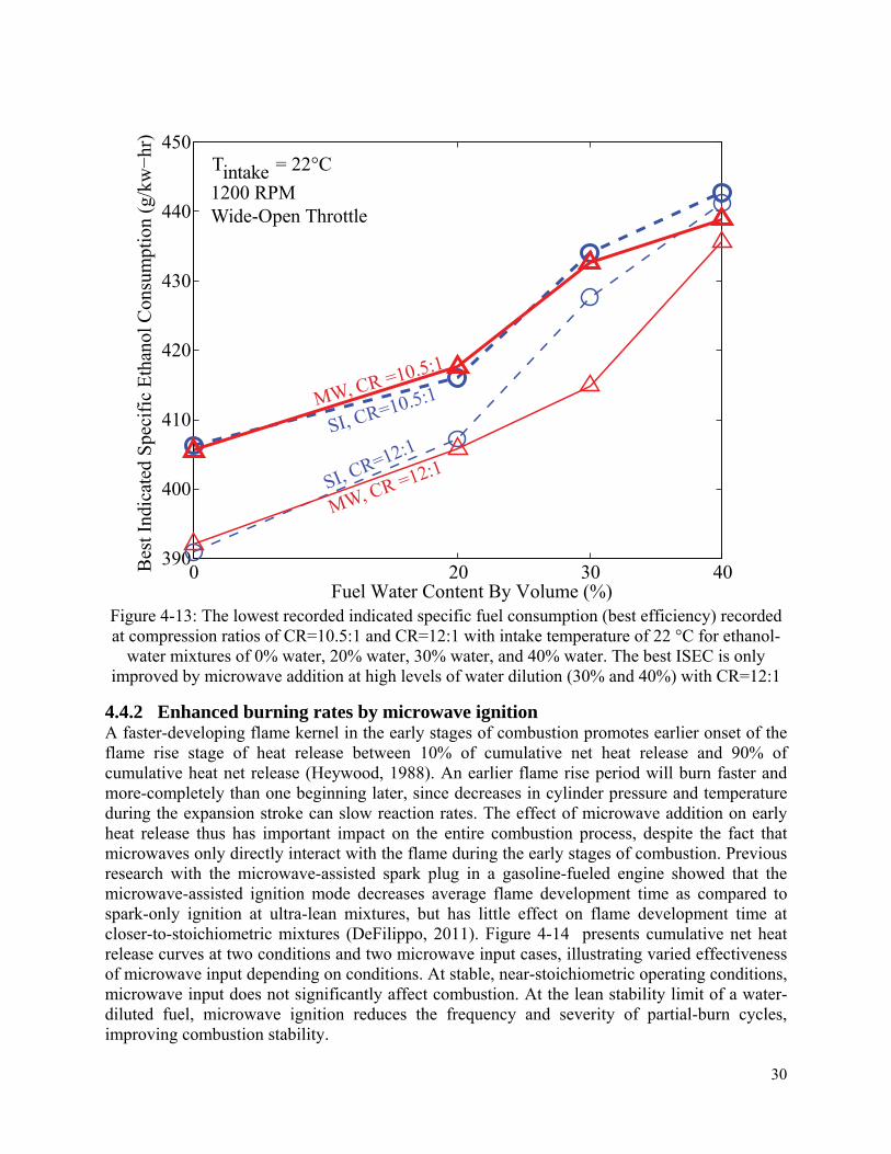
30

Figure 4-13: The lowest recorded indicated specific fuel consumption (best efficiency) recorded at compression ratios of CR=10.5:1 and CR=12:1 with intake temperature of 22 °C for ethanol-

water mixtures of 0% water, 20% water, 30% water, and 40% water. The best ISEC is only improved by microwave addition at high levels of water dilution (30% and 40%) with CR=12:1

4.4.2 Enhanced burning rates by microwave ignition A faster-developing flame kernel in the early stages of combustion promotes earlier onset of the flame rise stage of heat release between 10% of cumulative net heat release and 90% of cumulative heat net release (Heywood, 1988). An earlier flame rise period will burn faster and more-completely than one beginning later, since decreases in cylinder pressure and temperature during the expansion stroke can slow reaction rates. The effect of microwave addition on early heat release thus has important impact on the entire combustion process, despite the fact that microwaves only directly interact with the flame during the early stages of combustion. Previous research with the microwave-assisted spark plug in a gasoline-fueled engine showed that the microwave-assisted ignition mode decreases average flame development time as compared to spark-only ignition at ultra-lean mixtures, but has little effect on flame development time at closer-to-stoichiometric mixtures (DeFilippo, 2011). Figure 4-14 presents cumulative net heat release curves at two conditions and two microwave input cases, illustrating varied effectiveness of microwave input depending on conditions. At stable, near-stoichiometric operating conditions, microwave input does not significantly affect combustion. At the lean stability limit of a water-diluted fuel, microwave ignition reduces the frequency and severity of partial-burn cycles, improving combustion stability.

0 20 30 40390

400

410

420

430

440

450

Fuel Water Content By Volume (%)

Bes

t Ind

icat

ed S

peci

fic

Eth

anol

Con

sum

ptio

n (g

/kw−

hr)

= 22°CTintake1200 RPMWide-Open Throttle

MW, CR =12:1SI, C

R=12:1

MW, CR =10.5:1

SI, CR=10.5:1

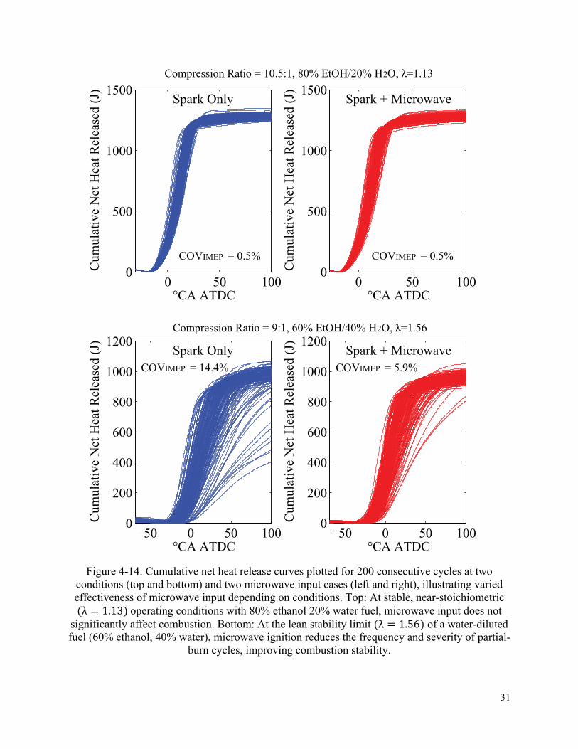
31

Figure 4-14: Cumulative net heat release curves plotted for 200 consecutive cycles at two conditions (top and bottom) and two microwave input cases (left and right), illustrating varied effectiveness of microwave input depending on conditions. Top: At stable, near-stoichiometric λ 1.13 operating conditions with 80% ethanol 20% water fuel, microwave input does not

significantly affect combustion. Bottom: At the lean stability limit λ 1.56 of a water-diluted fuel (60% ethanol, 40% water), microwave ignition reduces the frequency and severity of partial-

burn cycles, improving combustion stability.

−50 0 50 1000

200

400

600

800

1000

1200

°CA ATDC

Cum

ulat

ive

Net

Hea

t Rel

ease

d (J

)

Spark Only

−50 0 50 1000

200

400

600

800

1000

1200

°CA ATDC

Cum

ulat

ive

Net

Hea

t Rel

ease

d (J

)

Spark + Microwave

0 50 1000

500

1000

1500

°CA ATDC

Cum

ulat

ive

Net

Hea

t Rel

ease

d (J

)Spark Only

0 50 1000

500

1000

1500

°CA ATDCC

umul

ativ

e N

et H

eat R

elea

sed

(J)

Spark + Microwave

Compression Ratio = 10.5:1, 80% EtOH/20% H2O, λ=1.13

Compression Ratio = 9:1, 60% EtOH/40% H2O, λ=1.56

COVIMEP = 0.5% COVIMEP = 0.5%

COVIMEP = 14.4% COVIMEP = 5.9%

32

4.4.3 Factors influencing microwave effectiveness The microwave-assisted spark plug has been shown to improve engine stability when air-fuel mixtures are diluted with air or if the fuel is diluted with water, but little benefit is observed with the microwave-assisted ignition mode when conditions are already-stable. Past reports have not explained this observation. In an engine environment, it is difficult to isolate the variables contributing to the observed diminished microwave effects at closer-to-stoichiometric conditions. For example, in a fast-burning, near-stoichiometric fuel-air mixture, the conditions for combustion could simply be strong enough that microwave enhancement is insignificant relative to the unaided burning rate of the spark-ignited mixture. Upon further consideration, the important point may not be that the microwave effects are less relevant when chemistry is faster, but perhaps instead that microwave effects diminish because pressures are higher at the time of spark. A faster-burning mixture requires less burn duration, so the spark is fired closer to top-dead-center. The temperature and pressure are thus higher at time of spark because the spark is initiated later in the compression stroke. The advantage of the present multi-parameter study is that the effects of individual parameters can be studied.

The percent enhancement of flame development time by microwaves will be used in the following subsections as a metric for microwave effectiveness. The percent enhancement by microwaves is determined from the spark-only flame development time ( ) and the microwave-assisted flame development time using equation (4.8).

EnhancementofFDTby microwaves % 100 (4.8)

4.4.3.1 Effect of kernel time near the electrode on microwave enhancement One potentially important factor determining microwave effectiveness is the time during which the flame kernel is near the spark plug. A slower-developing flame resides near the spark plug longer, allowing more absorbed microwave energy since microwave power attenuates strongly with distance from the plug. Figure 4-15 plots microwave-assisted flame development time against spark-only flame development time for equivalent engine operating conditions. When combustion is robust and flame development time is short, the addition of microwaves does not accelerate flame development. At longer flame development times, microwaves accelerate flame development relative to spark-only ignition. The observed increased effectiveness of microwave enhancement at longer flame development times may indeed be due in part to the increased amount of time that the flame is near the electrode, but other potentially-important variables such as pressure and temperature at time-of-spark also change as flame development time changes.

33

Figure 4-15: Microwave-assisted flame development time (FDT) vs. spark-only FDT with conditions otherwise held constant (left). The figure on the right shows the same data in terms of

percent enhancement of microwave FDT vs. spark only FDT. When FDT is short, microwave addition has negligible effect compared to spark-only ignition. Microwaves effectively enhance

more-dilute mixtures that have longer spark-ignited flame development times.

4.4.3.2 Resolving impact of temperature and pressure on microwave effectiveness Isolating the effects of temperature from the effects of pressure in an internal combustion engine can be difficult because temperature and pressure increase together as the piston compresses the fuel-air mixture before spark. Figure 4-16 presents a contour plot of FDT enhancement by microwaves against pressure and temperature at time-of spark for all points with COVIMEP < 50%. The strong coupling between pressure and temperature is apparent by the narrowness of the regime; however there is approximately a 50 °C span of temperature at time of spark for each pressure at time of spark. Microwaves most-effectively enhance ignition at low temperature and low pressure, with the strongest enhancement observed only at the lowest pressure. The vertical banding of the enhancement contours implies that pressure is likely more important than temperature in determining microwave effectiveness.

2 4 6 8 100

2

4

6

8

10

12

14

16

Spark-Only Flame Development Time (ms)

Enh

ance

men

tof

FDT

by

Mic

row

ave

[%]

E100,W0E80,W20E70,W30E60,W40

2 3 4 5 6 7 8 9 102

3

4

5

6

7

8

9

10

Spark-Only Flame Development Time (ms)

Mic

row

ave-

Ass

iste

d F

lam

e D

evel

opm

ent T

ime

(ms)

E100,W0E80,W20E70,W30E60,W40

34

Figure 4-16: The percent enhancement of FDT by microwaves relative to spark-only FDT is plotted against temperature and pressure at time of spark for all data with COVIMEP < 50%.

Microwaves most-effectively enhance ignition at low temperature and low pressure. The strong coupling between pressure and temperature is apparent by the narrowness of the regime.

One way to isolate the effects of mixture composition from the effects of mixture pressure and temperature when determining the factors contributing to microwave effectiveness is to vary spark timing from advanced to retarded while holding all other engine conditions constant. Figure 4-17 shows the results of such an exercise at a CR =9:1; TIntake=60.5 °C; λ=2.08; 80% ethanol 20% water fuel, and 1200 RPM engine speed. When timing is advanced and pressure is low at time-of-spark, microwave ignition significantly enhances flame development time as compared to spark-only ignition. When timing is retarded and pressures are higher at time-of-spark, observed microwave effects diminish, with the microwave-assisted flame development time converging to approximately equal the spark-ignited flame development time. This observed diminished microwave effectiveness at elevated pressures is consistent with the observation that microwaves do not significantly enhance close-to-stoichiometric engine operation and also is consistent with the predictions of numerical models presented in the following chapters which show diminished effects of electron-energy enhancement of ignition at higher mixture pressures. Electron mean free paths in higher-pressure mixtures are shorter, reducing the amount of energy that can be delivered by microwaves to electrons between collisions and thus limiting the possibility for microwave enhancement of chemistry as long as microwave power is held constant.

35

Figure 4-17: For a fixed engine operating condition (CR =9:1; TIntake=60.5 °C; λ=2.08; 80% Ethanol 20% water, 1200 RPM) adjusting spark timing varies the in-cylinder pressure at time of spark. When timing is advanced and pressure low at time-of-spark, microwave ignition strongly

enhances flame development time compared to spark-only ignition. When timing is later and pressures are higher at time-of-spark, diminished microwave effects are observed through

convergence of flame development times.

4.4.3.3 Correlating microwave enhancement to in-cylinder parameters For engineering applications, it would be useful if microwave enhancement correlated to in-cylinder properties. Simple theory would suggest that enhancement by microwaves should relate to the energy transferred to the mixture by the microwaves, which should be proportional to the time that the flame receives an energy source times the rate of energy input. The energy input

rate through joule heating is proportional to the square of reduced electric field , which is

the electric field, , divided by the gas number density, (Lelevkin, 1992). The ideal gas law is applied for gas number density. Assuming that the microwave source remains on for longer than the flame kernel is near enough to the electrode that it can absorb energy, the time of energy input can be assumed proportional to the inverse of the laminar flame speed, , , giving a relation roughly proportional to energy coupled into the mixture as in (4.9).

~ ~ , ∙

EN

∙

(4.9)

As mentioned in section 4.3.6, flame speed information for ethanol-water mixtures was unavailable, so flame speed correlations for pure ethanol , , , , equation (4.7), were applied to all ethanol water mixtures with the understanding that the flame speed correlation will over-predict flame speeds and that the equivalence ratio dependence utilized in the correlation

3 3.5 4 4.5 5 5.5 65.5

6

6.5

7

7.5

Pressure at time of spark [bar]

Fla

me

Dev

elop

men

t Tim

e [m

s]

Spark OnlyMicrowave-Assisted

36

for 100% ethanol may not accurately predict the equivalence ratio dependence of the water-diluted fueling case. Correlations may improve not only through better estimates of flame speed, but also through improvements in calculating in-cylinder heat transfer and mass loss so that in-cylinder temperature can be more-accurately calculated from pressure data using equation (4.6). Figure 4-18 plots the fractional enhancement of flame development time by microwaves compared to spark-only when microwave energy absorption time is governed by flame speed.

Figure 4-18: Fractional flame development time enhancement by microwaves for all cases with 50%plotted against a factor calculated from in-cylinder properties , , for

each fueling case presently under study, assuming that the time for energy input by microwaves is proportional to the inverse of flame speed. The 100% ethanol case shows a near-linear dependence of enhancement, but the water-diluted cases do not show such a strong trend.

If the flame kernel is near the electrode for a time period greater than the microwave duration, , then the flame speed term will drop out of (4.9), and the resulting expression for

energy input will be given by (4.10).

~ ∙

EN

∙

∙

(4.10)

0 1 2 3 4 5 6 7

x 108

0

5

10

15

SL ,E100−1 (ms/cm) x N

Gas−2 (cm3/mol)2

Fra

ctio

nal F

DT

Enh

ance

men

t (%

)

100% Ethanol

0 2 4 6 8 10 12

x 108

0

2

4

6

8


Gas−2 (cm3/mol)2

Fra

ctio

nal F

DT

Enh

ance

men

t (%

)

80% Ethanol

0 0.5 1 1.5 2 2.5 3 3.5

x 108

0

2

4

6

8

10


Gas−2 (cm3/mol)2

Fra

ctio

nal F

DT

Enh

ance

men

t (%

)

70% Ethanol

0 0.5 1 1.5 2 2.5 3

x 108

0

1

2

3

4

5

6

7


Gas−2 (cm3/mol)2

Fra

ctio

nal F

DT

Enh

ance

men

t (%

)

60% Ethanol

37

Figure 4-19: Fractional flame development time enhancement by microwaves for all cases with 50%plotted against a factor calculated from in-cylinder properties , , for

each fueling case presently under study, assuming that the time for energy input by microwaves is proportional only to the microwave input duration. The 100% ethanol case still shows a near-

linear dependence of enhancement, and the 80% ethanol cases appear to have more-linear behavior than in Figure 4-18.

4.5 Conclusions A matrix of tests was conducted on a single-cylinder CFR engine comparing the microwave-assisted spark ignition mode to the spark-only ignition mode with wet-ethanol as a fuel. The microwave-assisted spark ignition mode allows stable engine operation in regions with higher dilution than possible with spark-only ignition. Microwave-assisted ignition can improve stability when operation destabilizes due to charge dilution with both air and water. The observed diminished effects of microwave-assisted spark ignition at near-stoichiometric conditions can be explained by elevated in-cylinder pressures that diminish microwave effectiveness. Combustion enhancement by microwaves appears more-strongly dependent on pressure than temperature.

0 5 10 15

x 107

0

5

10

15

NGas−2 (cm3/mol)2

Fra

ctio

nal F

DT

Enh

ance

men

t (%

)100% Ethanol

0 5 10 15

x 107

0

1

2

3

4

5

6

NGas−2 (cm3/mol)2

Fra

ctio

nal F

DT

Enh

ance

men

t (%

)

80% Ethanol

0 5 10 15

x 107

0

2

4

6

8

NGas−2 (cm3/mol)2

Fra

ctio

nal F

DT

Enh

ance

men

t (%

)

70% Ethanol

0 5 10 15

x 107

0

1

2

3

4

5

6

7

N−2 (cm3/mol)2

Fra

ctio

nal F

DT

Enh

ance

men

t (%

)

60% Ethanol

Gas

38

5 Plasma-Assisted Ignition Model Development Further development of practical combustion applications implementing microwave-assisted spark technology will benefit from predictive models which include the plasma processes governing the observed combustion enhancement. In addition to the fluid mechanics and chemical kinetics governing traditional combustion systems, modeling a microwave-enhanced combustion system requires modeling interactions between electromagnetic waves and charged particles and electron interactions with neutral and charged particles. Electron-neutral interactions in a plasma system can significantly increase concentrations of electronically-excited and vibrationally-excited species, so the chemical kinetic mechanism must be expanded with reactions for plasma-produced species. This chapter introduces the governing equations and chemical mechanism used in the present well-mixed reactor modeling approach.

5.1 Governing Equations for Well-Mixed Reactor Model The present numerical model solves time evolution of a constant pressure well-mixed reactor. A modified version of the CHEMKIN II (Kee et. al, 1989) developed for the present analysis not only solves equations for gas phase energy conservation and chemical species evolution, but also electron energy conservation. The electron energy equation includes a source term for energy input to the electrons that can take various forms depending on the plasma of interest.

5.1.1 Electron energy equation The electron energy evolution is governed by equation (5.1)

1

, , (5.1)

is the electron temperature, is the gas phase temperature, is the gas density, is the electron mass fraction, , and , are the electron heat capacities at constant volume and pressure respectively, is the universal gas constant, is the molecular weight of electrons, and is the chemical source term for electrons. The first term on the right-hand side accounts for the work done by the electrons. The second term on the right-hand side accounts for the energy required to raise the temperature of a newly liberated electron from the gas temperature to the electron temperature. ,detailed in (4.2) accounts for energy transfer from electrons to heavier gas molecules through elastic collisions. , described in (5.3) accounts for the energy transfer from electrons to heavier gas molecules through inelastic collisions. , is the user-specified source term that models the energy deposited to the electrons from the electromagnetic waves.

, 2 ∙ ,

#

∙ ∙ ~ (5.2)

In the expression for , the average translational energy difference between electrons and

gases equals the electron constant volume heat capacity, , , times the difference

between electron temperature, ,and gas temperature, in Kelvin. The fraction of energy transferred per collision is twice the ratio of the electron mass to the mass of species , . The number densites of electrons and species are and , respectively, and divided by

39

Avogardro’s number, , produces units of moles per volume. Multiplying the molar concentrations of electrons and species by the rate coefficient for elastic interaction between electron and species , , , gives the volumetric rate of elastic collision. Multiplying the fraction of energy transferred per collision by the collision rate and the average translational energy difference between gas and electrons gives the rate of energy transfer through elastic collisions.

The term is found by summing over the energy change, Δ ,multiplied by the net rate of progress of all electron reactions, , as in (5.3) where is the reaction rate coefficient of reaction , is the concentration of species , and is the stoichiometric coefficient of

reactant species .

Δ

#

(5.3)

5.1.2 Electron energy source term The present model allows specification of the electron energy source, , using a variety of relations depending on the plasma of interest. The simplest method allows user specification of a

constant volumetric source term over a specified duration, with units , which can be useful

for discharges when the energy input rate has been calculated before the kinetics calculation. A drawback to the constant source method is that since input rate is independent of electron concentration, if electron density becomes very low, the average energy input per electron will be very high, resulting in very high electron temperatures since total electron heat capacity . The user must thus exercise care when applying the constant source method, ensuring that conditions are set in a physically-appropriate manner before running the simulation.

A second allowable energy input method treats energy input as proportional to the electron concentration, eliminating the issue by which the electron energy becomes very high when electron concentration is low. Energy input proportional electron density is appropriate for several plasma cases, including low-density inductive discharges or cases when collisionless heating of electrons by electromagnetic waves is the dominant energy transfer mechanism.

A third model for energy input to the electrons, , , uses equations for ohmic heating of plasma (Lieberman, 2005). Ohmic power input is proportional to the square of the absolute value

of the electric field, , the DC conductivity, , and a ratio including the electron-neutral collision frequency, , and the driving frequency of the source, , as in (5.4)

,

12

12

~ (5.4)

DC conductivity, , depends on the electron concentration per unit volume, , the electron neutral-collision frequency, , as well as constants , the charge of an electron, 1.60210 , and , the electron mass, 9.11×10-31 kg.

40

The ohmic heating model for the electron energy source can also apply to the energy input through electromagnetic wave absorption by plasma. When the ionization degree is low such that the refractive index, , approaches unity, the absorption coefficient, , in the Bouguer law expression for attenuation of electromagnetic wave with energy flux / ), becomes proportional to plasma conductivity as in (Fridman, 2011.) Constants include , the permittivity

of free space 8.854 10 and , speed of light in a vacuum 2.9979 10 / .

∙∙ ∙

∙

→ 1, ,∙ ∙

~

(5.5)

Both ohmic heating and Bouguer law absorption are proportional to a specified constant, electron density, , and the ratio of collision frequency to the sum of the squares of collision frequency and driving frequency, ,making the ohmic energy input appropriate for a range of

discharges.

The present energy input specification methods do not include stochastic heating methods through which electrons gain energy through reflection off of sheaths. The model currently lacks spatial resolution over which the Poisson equation can be solved and any sheaths can be resolved, but fortunately, for the relatively high pressures of interest in combustion applications, stochastic heating will typically be small relative to ohmic heating since electron collision frequencies are high and mean free paths are short relative to discharge dimensions.

Even with the many ways that the present energy input specification methods can be given dimensionally-correct parameters of interest, it is difficult to precisely assign the numerical energy input conditions to match experimental parameters without spatial resolution of charge distribution or electromagnetic wave propagation into the plasma. The available energy input models are useful for identifying trends in combustion enhancement mechanisms through chemical kinetics when various magnitudes of energy input are applied and electron concentration is either high or low. Future models will benefit from advanced spatial resolution of electric field, wave propagation, and charged particle distribution for quantitative predictive modeling relating physically-relevant source parameters to observed combustion enhancement.

5.1.3 Gas energy equation The gas energy equation (5.6) solves for the evolution of the temperature of the homogeneous mixture, including terms accounting for energy exchange with electrons.

1, (5.6)

and are the density and constant pressure heat capacity of the gas phase (not including

electrons). The work done by the mixture is accounted by the term. The term

accounts for heat release from chemical reactions. The third, fourth, and fifth terms on the right-

41

hand side are the same as those in the electron energy equation. The final term, , , allows a user-specified amount of energy to directly add energy to the gas molecules.

5.1.4 Chemical species evolution Concentrations of chemical species and electrons in the modeled zero-dimensional homogeneous mixture evolve based upon their concentrations and the specified reaction rate coefficients. The only difference between the chemical species evolution scheme of the present model and that of a traditional combustion kinetics solvers such as CHEMKIN (Kee et. al, 1996) or Cantera (Goodwin, 2003) is that rate coefficients in the present model can depend upon electron temperature in addition to gas temperature and pressure. Specifics of chemical species evolution through kinetics calculations in a gas-phase system are well described in Warnatz (2006) but will be briefly discussed here for the sake of completeness.

Consider a simple reaction mechanism containing chemical species A, B, C, D, and E evolving based upon elementary reactions Reaction 1 and Reaction 2 below, with species concentrations specified by brackets, such as B ~ / . Reaction rate coefficients for each reaction are specified by the letter , such as _1~ / ∙ . The rate of a reaction is then the concentration of the products multiplied by the reaction rate coefficient, giving a source term with units / ∙ .

Reaction 1: A B→C D

Reaction2:C D → E

d Adt

d Bdt

∙ A ∙ B

d Cdt

d Ddt

∙ A ∙ B C ∙ D

d Edt

C ∙ D

(5.7)

With the time rate of change of chemical species concentrations depending on the species concentrations, the chemical kinetics system is described by a system of differential equations. In the case of large mechanisms with many species and reactants, analytical solution becomes impossible, and the kinetics must be solved numerically. The differential equations from the mechanism of (5.7) can be rewritten as:

42

d Adtd Bdtd Cdtd Ddtd Edt

0 0 00 0 0

00

0 0 0

ABCDE

(5.8)

Equation (5.8) can be written in the form of (5.9), which is a simple linear ordinary differential equation (ODE) with vectors and containing the source terms and the concentrations, respectively, and the matrix containing the reaction rate coefficients (Warnatz, 2006.)

(5.9)

The timescales of reactions in a large mechanism can span several orders of magnitude, making the differential equations stiff. Time advancement of equation (5.9) is thus best solved using a stiff implicit ODE solver. The present model utilizes DASAC (Caracotsios, 1985). It is worth noting that the only complication added to chemical species evolution with the addition of electron-temperature-dependence is that some of the rate coefficients in matrix will be functions of electron temperature, instead of gas temperature, . The following subsections describe the compilation of reactions that make up the present chemical mechanism for species evolution in a combustion system enhanced by high-energy electron interactions.

5.2 Gas-Phase combustion reactions The base combustion model contains a series of reactions for modeling the gas-phase oxidation of methane in air as well as the evolution of atmospheric compounds including oxides of nitrogen and ozone. The base combustion model is the mechanism of Warnatz (1997) for high-temperature (T > 1200 K) oxidation in H2–CO–C1–C2–O2 systems. The mechanism includes 35 species and 162 reactions. Since pressures change dynamically during a given simulation for the internal combustion applications of interest, the Kassel formulation reactions of the Warnatz mechanism have been replaced with updated reaction rates coefficients that contain pressure dependence (Smith, GRI-Mech), (Mehl et. al, 2011). The mechanism has been supplemented with a nitrogen-oxygen reactions for the formation of oxides of nitrogen (Smith, GRI-Mech), and reactions for ozone (O3) formation and destruction (Sharipov and Starik, 2012). Future mechanism updates may benefit from an updated gas-phase reaction mechanism, however the current base mechanism was selected because the flame-ionization mechanism of Prager (2007) was designed for use with the present gas phase combustion model.

5.3 Electron impact reactions The majority of energy transferred to plasma by an electromagnetic discharge is first received by free electrons because their low mass results in strong acceleration from an applied electromagnetic force. Once electrons receive energy from the discharge, they transfer energy to other particles and initiate chemical processes through electron impact reactions. Determining the rate at which electron impact reactions proceed is thus essential for modeling plasma-assisted

43

combustion. The rate of an electron impact reaction depends on the available electron energy and the collisional cross section of interaction. The following subsections explain the presently-employed methods for determining electron energy (Figure 5-1, Left), the cross section of interaction (Figure 5-1, Right), and the combination of these two important quantities towards calculating the rate of reaction.

Figure 5-1. The rate of an electron impact reaction depends on the product of the Electron Energy Distribution Function which varies with Electron Temperature ( ) [Left], and an experimentally-determined impact cross section for the specific impact process [Right].

5.3.1 Electron energy accounting The first step in determining the rate of an electron impact processes is through consideration of the electron energy available for initiating the processes. Since electrons have no internal degrees of freedom, the energy, , of an individual electron consists entirely of kinetic energy. The energy of an electron is thus proportional to its mass, 9.1095 10 , and the square of the electron velocity, ; with the equation for electron energy given in equation (5.10).

12

(5.10)

For an ensemble of electrons in a system of interest, there will be some electrons with high velocities and thus high energy, and some electrons with low velocities and correspondingly low energies. The electron energy distribution function (EEDF), , contains information on the probability that an electron in the system will have energy between and . Integration of the product of the EEDF and the electron energy over all possible electron energies gives the average energy of the electrons,⟨ ⟩, in the system as in (5.11). The average energy can be converted to temperature units through the Boltzmann constant, 1.3807 10 / . The electron temperature, , will frequently be used as a measure of overall electron energy in the present model.

10 -1

10 0

101

10210

-3

10 -2

10 -1

10 0

10 1 Maxwellian EEDF

Electron Energy [eV]

EE

DF

[eV

-1]

T e =1500 K

Te =16000 K

Te=32000 K

10-1

100

10 1

10210

-3

10-2

10-1

100

101

Vibrational Excitation of N2

Electron Energy [eV]

Cro

ss S

ectio

n [1

0-16 c

m2 ]

44

∙ ⟨ ⟩32

(5.11)

The electron energy distribution function can take several forms. A common assumption is that electrons in a system are in thermal equilibrium with each other, in which case the electron energy distribution can be described by the Maxwellian distribution given in (5.12)

2/

exp (5.12)

Unfortunately, the EEDF may deviate from the Maxwellian, as electrons of specific energy ranges will lose energy through resonant collisions with gas molecules. The Boltzmann transport equation, which tracks the theoretical evolution of an ensemble of particles in six-dimensional phase space (position and velocity) requires significant simplification for practical calculation of the electron energy distribution function and the resulting electron-impact reaction rates in non-thermal plasma. Hagellar and Pitchford (2005) released a user-friendly, freely-available code called BOLSIG+ that solves the two-term expansion of the Boltzmann equation. The most general form of the Boltzmann transport equation for a system of electrons is in Equation (5.13), where is the electron energy distribution in phase space, is the velocity vector, is the elementary charge of an electron, is the mass of an electron, is the velocity gradient operator, and accounts for changes in due to collisions.

∙ ∙ (5.13)

Hagelaar and Pitchford (2005) simplify equation (5.13) by first assuming spatial uniformity in the electric field and collision probabilities, making symmetric in velocity space around the electric field direction, and only varying along the electric field direction in position space. The equation is then converted to spherical coordinates so that becomes a function of , , , , where is the angle between the velocity and the field direction and is the position along the field direction. The time dependence is simplified by considering that the electric field and electron distribution are either steady-state or governed by high-frequency oscillation. The two-term approximation simplifies the spatial dependence in by expanding into an isotropic part,

, and an anisotropic perturbation, as in equation (5.14)

, cos , , , , , , cos (5.14)

Substituting (5.14) into a spherical coordinate version of (5.13), multiplying by Legendre polynomials and integrating over cos produces equations for the isotropic, , and anisotropic,

, parts of the energy distribution function, with N the neutral gas density (1/ ), E the electric

field ( / ), and the constant . used for convenient conversion between energy and

velocity units (Hagelaar and Pitchford, 2005).

3 3

(5.15)

45

The term includes the change in due to all collisions, including elastic collisions, excitation collisions, ionization, attachment, and electron-electron collisions. The term on the right hand side of the anisotropic equation refers to the total momentum transfer cross section for all collisions with gases. Additional assumptions regarding the temporal and spatial dependence of

and are made, separating the energy dependence of the distribution from its time and space dependence so that the energy distribution is constant in time and space, and the electron density varies based on the net electron formation and destruction rate. After a series of combinations, the EEDF equation reduces to an advection-diffusion type equation (5.16) , with the term an advective part corresponding to cooling through elastic collisions with lower-energy particles, and a diffusive part, corresponding to heating by the electric field and through elastic collisions with higher-energy particles. The term includes all inelastic collision processes, with energy subtracted and added at various locations in energy space depending on the energy of the participating electron before and after a given process.

(5.16)

Equation (5.16) is solved numerically for the energy distribution by discretizing into cells over energy space, with the value of the distribution function in each cell relating to the value of the distribution function in other cells. The terms are then discretized using various schemes and implicitly evaluated. Solution to these equations are accomplished through user-friendly interfaces, either through a Fortran-based command line interface called ZDPlasKin (Zero-Dimensional Plasma Kinetics, http://www.zdplaskin.laplace.univ-tlse.fr/ ) or using the BOLSIG+ graphical user interface, available at http://www.bolsig.laplace.univ-tlse.fr/. For the present analysis, electron-electron collisions are neglected due to the low-ionization degree of the flame plasmas of interest. Solution of the energy distribution function requires information on the cross section of interaction for relevant electron impact processes, discussed in the following section.

46

Figure 5-2 Example of oxygen ionization rate coefficients calculated using BOLSIG+ compared with rate calculated assuming Maxwellian EEDF. At low ionization levels, 10 ,

neglecting electron-electron collisions is a suitable approximation. At high ionization levels, the calculated rate approaches the Maxwellian prediction.

5.3.2 Electron impact cross sections Electron-energy-dependent impact cross sections for each reaction, , have units of area, and are available in the literature for many of the fuel, oxidizer, intermediate, and product species present in gas-phase combustion systems. Physicists determine cross sections using experimental methods including measurement of electron energy loss, detection of collision products, beam attenuation methods, merged beam methods, and swarm experiments (Itikawa, 2007).

Electron impact reaction types include elastic collisions and inelastic collisions, with inelastic collisions including ionization, dissociation, excitation, and attachment reactions. Elastic collisions transfer momentum between the electron and translational modes of the target particle, but since momentum and energy must both be conserved during an elastic collision, the amount of energy transferred by an electron through a single elastic collision is on the order of the mass ratio of the electron to the target particle. Atoms can undergo electronic excitation, while polyatomic molecules may undergo rotational, vibrational, or electronic excitation. An elastic collision between an electron and an atom within a molecule cannot likely transfer sufficient energy to excite a vibrational quantum due to the same requirement for momentum and energy conservation that limits elastic energy transfer, so vibrational excitation typically proceeds through an intermediate state. First, the electron attaches to the molecule through a resonant process, forming an unstable negative ion in what is called an auto-ionization state. The electron then detaches with a lower energy and the molecule is left in a vibrationally-excited state. Dissociation reactions result in the formation of multiple particles by breaking chemical bonds between atoms, typically by electronic excitation into a repulsive molecular state or to an

Increasing Ionization Degree

47

attractive state which then transitions to a repulsive state. Attachment reactions reduce the pool of free electrons as a negative ion is formed, with the excess energy of the electron typically accounted for through breaking of a molecular bond, in a process called dissociative attachment, or through collision with a third body, in a process called three-body attachment. Ionization reactions release an electron from the target particle, and if the incident electron possesses sufficient energy, the ionization may be accompanied by dissociation of the molecule in a process called dissociative ionization.

The cross sections used in the present work come from a range of sources. A recent series of papers by the Itikawa research group provide well-referenced compilations of measured cross sections for electron impact processes of oxygen (2009), nitrogen (2006), H2O (2005), CO2 (2002), and hydrogen (Yoon, 2008.) The Itikawa cross sections were not published as “complete” sets calibrated for discharge calculations, however. A convenient digitized database of complete sets of electron impact cross sections has been compiled by the Laboratoire Plasma et Conversion d'Energie at the Universite Paul Sabatier in Toulouse, France (LXCAT, short for ELECTron SCATtering database, www.lxcat.net), and includes digitization of the Phelps cross sections, and the cross section compilations of A.V. Phelps retrieved from LXCAT are used as a framework for cross section sets of oxygen (Lawton and Phelps, 1978) and nitrogen (Phelps and Pitchford, 1985), and the cross section set of Hayashi retrieved from LXCAT is used for methane (CH4). Cross sections for CH1-3 were generated using the formulas of Janev and Reiter (2005). The sources for all cross sections used in the present effort are given in Table 5-1. Elastic collisions, rotational excitation, vibrational excitation, and high-energy electronic excitation are taken from Phelps since the complete cross section set has been optimized for agreement with experiments. Unfortunately, complete electron-impact cross section sets are not presently available for ethanol or hydrocarbon chains longer than C3H8 (propane), so the present modeling focuses on plasma-assisted ignition of methane-air mixtures. The following sections relate some details of how the cross section sets of Phelps have been modified for the present model and how cross sections for electron impact with excited species were calculated.

48

Table 5-1. Electron Impact Target Species and Cross Section Sources

Target Species Number

of Impact Reactions

Metastable Excited states included in

present model

Ions formed through

attachment and ionization

Source

O2 13 Vibrational levels 1-4, O Δ , O Σ , O Σ , O

O2+ O+

O2- O-

(Lawton, 1978) (Ionin, 2007)

(Itikawa, 2009)

N2 26 Vibrational levels 1-8, N Σ , N Π , N Σ , N Π

N2+ N+

(Itikawa, 2006) (Phelps, 1985)

CH4 9 CH 13 , CH 24

CH4+

H- (Hayashi, 1987) (Janev, 2002)

CH3, CH2, CH 10, 9, 5 - CH3

+ CH2+

CH+ C+ (Janev, 2002)

(Morgan, 2013)

CO2 10 O CO+ CO2

+ (Itikawa, 2002) (Morgan, 2013)

H2O 16 - H2O

+ OH+ OH- H-

(Itikawa, 2005) (Morgan, 2013)

H2 17 - H2+ (Morgan, 2013)

CO 4 CO+ O+ C+ (Land, 1978), (Orient, 1987)

N Σ , N 1 O Δ , O Σ

O 1 , O

2, 5, 6, 7, 9, 2

- O2

+ O+ O2

- O-

N2+ N+

(Lawton, 1978) (Phelps, 1985) (Ionin, 2007)

(Itikawa, 2009)

5.3.2.1 Specifics of oxygen electron impact Electron impact with oxygen is essential in models of plasma-assisted combustion processes, as electron impact excitation and dissociation of oxygen is often cited as a primary cause of combustion enhancement (e.g. Ombrello, 2010). Fortunately, electron impact with oxygen has been highly-studied. Electron impact with oxygen can lead to gas heating through momentum transfer and rotational excitation processes. Oxygen molecules have a vibrational energy quantum of 0.1959 eV, with vibrational excitation occurring through narrow-peak resonant processes for incident electron energies below 1 eV, and through broad-peaked resonant processes for electron energies greater than 1 eV, with a maximum cross section for vibrational excitation near 10 eV. The first four vibrational states of oxygen are tracked in the present analysis. Oxygen molecules have two low-lying metastable singlet states with relatively long radiative lifetimes: O Δ has excitation energy of 0.977 eV and a radiative lifetime of almost 4000 seconds, and O Σ has excitation energy of 1.627 eV and a radiative lifetime of over 10 seconds (Capitelli, 2000). There are several higher electronic states with shorter lifetimes, as well: O Σ , O ′ Δ , and O Σ have similar excitation energies 4.34

49

eV, 4.262 eV, and 4.050 eV, resulting in their common treatment as a single state, a treatment applied in the present model. Excitation to the O Σ state, 6.120 eV and higher, most likely leads to predissociation into O and O(1D) (Capitelli, 2000). The complete cross-section set of A.V. Phelps also includes energy losses through electronic states with energies 8.4 eV and 9.97 eV, likely corresponding to the Schumann-Runge Continuum of the O Σ state.

Figure 5-3: Potential Energy vs. internuclear distance curves for oxygen states considered in the

present model. Adapted from Krupenie (1972).

For the present model, it is important that prediction includes not only energy loss, but also dissociation. The cross section compilation of Itikawa (2009) includes cross sections for total dissociation to neutral atoms, and the cross section set of Ionin (2007) includes cross sections for dissociation into ground state oxygen atoms. Itikawa provides no values below 13.5 eV, so the total dissociation cross section between 5.58 eV and 13.5 eV is assumed equal to the Ionin cross section. Above 13.5 eV, subtracting the Ionin ground state dissociation cross section from the Itikawa total dissociation cross section is assumed to produce the cross section for dissociation with one excited atom, O(1D). The cross sections of Phelps for energy loss excitations of 4.5 eV, 6.0 eV, 8.4 eV, and 9.97 eV are here treated as the sum of all high electronic excitation, and it is assumed that all 4.5 eV excitation results in the metastable but short-lived O Σ state. Next, any excitation to 6 eV is assumed to result in dissociation to ground-state neutrals wherever the 6.0 eV excitation curve and the Ionin neutral dissociation curve overlap. The remaining excitation to 6.0 eV is treated as an energy loss, presumably through radiation. The remaining dissociation to ground-state products is then presumed to occur through the 8.4 eV threshold reaction of Phelps. Additionally, all dissociation to an excited product is assumed to occur through the 8.4 eV excitation from Phelps, as the remaining cross section for total dissociation not already included in the 6.0 eV dissociation is at all points smaller than the cross section for

50

8.4 eV excitation provided by Phelps. After subtracting all cross sections for dissociation from the 8.4 eV excitation cross section, the remaining excitation is once again treated as energy loss. The 9.97 eV excitation cross section of Phelps is also treated as energy loss. The final results of the cross section transformations are shown in Figure 5-4. With these transformations, the total energy loss through electronic excitation of Phelps is preserved while also including recent cross sections that allow prediction of total dissociation.

Figure 5-4: Transformation of the cross sections for electronic excitation of A.V. Phelps at 4.5

eV, 6.0 eV, 8.4 eV, 9.97 eV preserves total electron energy loss while incorporating cross sections for dissociation to ground-state and excited-state oxygen atoms from Ionin (2007) and

Itikawa (2009). Final Cross Sections are tabulated in Appendix 3: Electron impact cross sections for upper-level electronic excitation of oxygen, in BOLSIG+ format.

5.3.2.2 Specifics of nitrogen electron impact Nitrogen molecules comprise the majority of molecules in a stoichiometric fuel-air mixture, making electron interaction with nitrogen highly likely. Vibrational excitation of nitrogen accounts for a great deal of electron energy loss in air discharges (Fridman, 2011), and excited states of nitrogen are important for triggering collisional electron detachment (Moruzzi and Price, 1974). The present model once again uses the A.V. Phelps compilation (Phelps and Pitchford, 1985) as a framework for collisional cross sections. Since rotational species modeling is not practical or easily experimentally-validated, it is here approximated that the rotational excitation of the Phelps cross section set results in gas heating, a reasonable approximation since the rotational heat capacity is included in the gas phase for the temperature range of interest in combustion applications. Several electronic states of nitrogen are rather short lived, however, so it is here approximated that only the , , ,and electronic states of excited nitrogen have stable existence. Excitation to the and states of N2 immediately become

51

in the present model, reducing the total number of species that must be considered. Similarly, the and states both become , and the and states both become

. Excitation to higher states of nitrogen leads to dissociation to a pair of nitrogen atoms in the present model (Kossyi, 1992).

5.3.2.3 Specifics of methane electron impact Electron impact that can potentially destabilize methane molecules may accelerate combustion. The complete cross sections of Hayashi are used for methane with some modification. The cross section set includes elastic energy transfer, vibrational excitation to the 2 and 4 modes (0.159 eV) and to the 1 and 3 modes (0.37 eV), excitation with a threshold of 7.9 eV, total ionization (threshold 12.9 eV), and total attachment (threshold of 7.9 eV.) It has been found that that all electronic excitation in methane leads to dissociation (Fuss, 2010), so the present model uses branching ratios and appearance potentials for methane dissociation as found in Janev and Reiter (2002) for identifying the distribution of dissociation products when the molecule undergoes excitation through the 7.9 eV threshold process. The most likely dissociation is to CH3 + H, with a branching ratio of 0.760, followed by CH2 + H2, then CH + H2 + H, and finally C + 2∙H2, with branching ratios of 0.144, 0.073, and 0.023 respectively. It is here approximated that all attachment is dissociative attachment with products CH3 and H-, for it is the least-endothermic attachment reaction to methane.

5.3.2.4 Specifics of CO2, H2O, and CO electron impact Combustion product species CO2 and H2O and intermediate species CO do not comprise a large fraction of the unburned gas mixture in ignition calculations, but concentrations of these two combustion products will be more important in practical flames and in engines with exhaust gas recirculation.

For CO2, electron impact cross sections utilize the Morgan (2013) complete cross section set retrieved from LXCat, with dissociation taken from Itikawa (2002). Using the same procedure as for molecular oxygen, the dissociative cross section of Itikawa (2002) was subtracted from the 10.5 eV electronic excitation set so that the total electron energy loss would match that of the Morgan cross section set. In the combustion model, all excitation processes to the many vibrational excitation modes of CO2 are considered electron energy loss processes, so that all vibrational excitation energy goes towards increasing the bulk gas temperature.

For H2O, a complete cross section including proper treatment of rotational electron impact that was compatible with the current BOLSIG+ solver was unavailable. Without rotational cross sections, H2O was considered to have zero concentration in the BOLSIG+ calculations so that the electron energy distribution function calculation would be unaffected. The cross section set of Itikawa (2005) was selected for the water impact processes, with rates calculated for BOLSIG+. After the rates are calculated, the rotational excitation collisions are combined into an effective momentum transfer reaction as described in section 5.3.4 so that rotational species need not be considered, with all rotational excitation collisions increasing the bulk gas temperature.

For CO, the complete cross section set of Phelps is utilized. After the BOLSIG+ calculation, all vibrational excitation is combined into an effective excitation to the first vibrational level of CO as described in section 5.3.4 so that electron energy loss rates are conserved. This leads to an overestimation of the total conversion rate to vibrationally-excited CO but reduces the number of

52

species that must be considered. Only the first vibrational level of CO is tracked, as the reaction involving CO as a reactant that most affects flame speed, CO + OH => CO2 + H (Warnatz, 2005) has an energy barrier smaller than the energy of the first vibrational excitation level of CO.

5.3.2.5 Electron impact with excited molecules Electron impact with an excited species can be important because such a collision can lead to stepwise processes such as ionization or dissociation through multiple electron collisions. First, an electron impacts a ground-state molecule, exciting the molecule to some metastable state. Next, a second electron impacts that excited species, resulting in another process. Consideration of the energy diagram in Figure 5-3 may make this idea clearer: say an electron excites an oxygen molecule to the 1.62 eV O Σ state. A second electron would then not need as much energy to further raise the potential energy of the molecule to an ionized state or a repulsive state leading to molecular dissociation. Ionin (2007) approximates cross sections for electron impact with excited species by shifting the cross sections by the amount of excitation to lower electron energies relative to the ground-state cross section as illustrated in Figure 5-5. Such an approach will not apply to resonant processes such as vibrational excitation, so in the present model, vibrational excitation of electronically-excited species is ignored.

Figure 5-5: Selected cross sections for electron impact with excited species are approximated by shifting the cross section by the energy of excitation, here shown for dissociation of an oxygen

molecule in ground and excited (1.62 eV) states.

5.3.3 Calculating the rate of an electron impact process Assuming a continuum treatment of electron transport and energy, kinetic theory states that the reaction rate coefficient, , of a process, , between a set of electrons and a set of gas particles

can be calculated by integrating the product of the electron velocity, /

, the electron-

energy-dependent collisional cross section for process , and the electron energy distribution function (EEDF), as in equation (5.17) (Meeks, 2000). Solving equation (5.17) at each electron temperature of interest will produce a rate coefficient dependent on electron temperature.

53

2

(5.17)

As discussed in section 5.3.1, the simplest treatment of electron energy is through assumption of a Maxwellian electron energy distribution function. Combining equation (5.17) with the distribution of equation (5.12) produces an electron temperature, , dependent rate coefficient that only requires information on the process cross section, as in (5.18).

8 1exp (5.18)

The Maxwellian distribution can produce a reasonable approximation of reaction rate, especially given the uncertainties in experimental cross sections. Solving the Boltzmann transport equation produces a more-accurate representation of the electron energy distribution of non-equilibrium plasma, however. When solving for the rate coefficient using the two-term approximation of the as in the present analysis, the electron-temperature-dependent rate coefficient of process is defined not only based on the cross section for the process, but also the gas composition and temperature, as these factors affect the electron energy distribution function.

As an engineering approximation in the present analysis, the electron-temperature-dependent rate coefficients are calculated before the main combustion calculation for a specified initial mixture composition. The approximation of a time-invariant EEDF is here made since the timescale of electron energy input is short compared to the timescale of combustion over which the mixture composition, temperature, and pressure significantly change. For improved accuracy at increased computational cost, the electron energy distribution function could be repeatedly calculated as the simulation progresses and the mixture composition and resulting shape of the EEDF changes.

Electron impact rate coefficients for the present model are calculated using a custom code that automatically generates input files for ZDPlasKin (Pancheshnyi, 2008), a Fortran 90 implementation of BOLSIG+, a two-term Boltzmann equation solver (Hagelaar and Pitchford, 2005). After running ZDPlasKin, the code converts the calculated rate coefficients into a format compatible with CHEMKIN. The algorithm for generating electron impact rates is as follows. First, the user sets the expected mixture composition and temperature. Next, the code is launched, the cross section database is converted to a BOLSIG+ compatible format, a master code and an input file are generated for ZDPlasKin, and ZDPlasKin calculates the rate coefficients for all electron impact reactions over a range of electron temperatures, outputting the reaction rates in a table. The table of rates vs. temperature is loaded into another custom code that curve-fits the reaction rates to the nine-parameter polynomial format of Janev (1987) and writes the nine polynomial coefficients, , into CHEMKIN-compatible format such that the rate coefficient is given by equation (5.19). A diagram of the algorithm used by the custom code for automatically converting cross sections and user-specified conditions is shown in Figure 5-6.

6.02214 10 ∙ exp ln (5.19)

54

Figure 5-6: A custom code automatically generates electron impact reaction rate coefficients that have been calculated using a Boltzmann transport equation solver, then curve fits the rates for conversion to CHEMKIN-compatible format for use in the present well-mixed-reactor code.

5.3.4 Combining electron impact processes with an “effective” rate An effective rate is employed which combines several processes into a single reaction such that total electron energy loss is conserved. An effective rate is generated so that the calculated rate of collisional energy transfer from electrons to gas particles is approximately the same as it would have been if rotational excitation and momentum transfer reactions were calculated using separate rates. Matching energy loss requires that the “effective reaction” has the same “stopping cross section” as the combination of the momentum transfer reaction and the rotational excitation reaction. Itikawa (2007) defines the stopping cross section, , as in (5.20).

Δ ∙ ∙ (5.20)

Here Δ is the energy transfer from the electron to the target molecule during the collision, and is the energy-dependent collisional cross section. For a quantized inelastic process such as

a rotational excitation, the energy transferred, Δ equals the difference in energy between the initial and final quantum states: for → rotational excitation, Δ 1.48 10 . For an

elastic momentum transfer collision in the laboratory frame where the target particle is at rest, the energy transferred from the electron in an elastic collision, Δ , is proportional to the energy of the electron, , the mass of an electron, , and the mass of the target particle, , as in (5.21).

Δ 2m

(5.21)

55

In the two-temperature well-mixed reactor code, electron-impact reactions can be flagged as momentum transfer reactions using the keyword MOME, in which case the elastic energy loss rate of a reaction, , , , is calculated using equation (5.22). , is proportional to the mass ratio of the electron and collisional partner just as in (5.21), but in the well-mixed reactor code, the assumption of a fixed target is no longer made, and the energy transfer is instead proportional to the difference between average electron temperature and average gas temperature, . Equation (5.22) additionally depends upon the electron heat capacity at

constant pressure, , ∙, and the reaction rate of the momentum transfer reaction per unit

volume, ∙

.

, 2m

, (5.22)

Figure 5-7: In the WMR code, the energy loss per collision of elastic reactions is dependent on gas temperature and electron temperature, as shown above, whereas rotational excitation energy is fixed. For nitrogen, the energy loss per elastic collision is lower than rotational excitation

collisions at electron temperatures below 200,000 K.

5.4 Modeling Excited Species Electron collisions with atoms and molecules will often excite the target particles into rotationally-excited, vibrationally-excited, or electronically-excited or states. Some excited particles quickly relax back to the ground state, while others maintain their elevated energy in a metastable state. The elevated internal energy of excited species can enhance chemical reactivity, especially for reactions with high activation energies. In the present model, rotationally-excited molecules are not treated separately from ground-state species, as the quantum of rotational

102

103

104

105

106

10-7

10-6

10-5

10-4

10-3

10-2

Electron Temperature, Te (K)

E (

eV p

er c

ollis

ion)

Elastic, Tgas

= 500 K

Elastic, Tgas

= 1500 K

Elastic, Tgas

= 2500 K

N2(J

0-2) Rotational Exc.

56

energy is so small that reliable data for rotational excitation is limited (Itikawa, 2009), and rotational-translational relaxation is so fast that rotational energy is typically in equilibrium with translational energy. It is thus modeled that all rotational excitation simply leads to an increase in the gas-phase temperature of the impacted species, an especially-appropriate approximation because the thermodynamic heat capacities presently utilized contain contributions from rotational excitation. For vibrational and electronic excitations, energy quanta are larger, lifetimes are longer, and experimental data is more plentiful. Predictive chemical kinetic models for plasma-enhanced combustion processes thus require accurate treatment of excited species, so the following subsections detail the present treatment of vibrationally- and electronically- excited species.

5.4.1 Thermodynamics of Excited Species The present model requires thermodynamic information (heat capacity, enthalpy, and entropy) as a function of temperature for each gas-phase species, information that is not readily-available for all excited species considered in the present model. Professor Burcat’s thermodynamic database (Burcat, 2005) tabulates data for many ground-state and ionized species in a polynomial form compatible with the present model, even including thermodynamics for the singlet oxygen molecule Δ and the singlet oxygen atom. For other excited species, thermodynamic information must be calculated or measured.

Advances in ab-initio electronic structure calculations allow for calculation of thermodynamic properties of electronically-excited molecules (e.g. Gaussian, M. J. Frisch et. al. 2009), but such calculations are outside the scope of the present investigation. Instead, it is assumed that heat capacities of excited species remain unchanged from their ground-state counterparts, and excited species simply have higher enthalpies of formation than their ground-state counterparts. The assumption of unchanged heat capacity after excitation is not completely accurate, as the vibrational constants of excited species may differ from those of the ground state, but with excited species only making up a small fraction of the total mixture, overall mixture heat capacity will not be impacted significantly.

5.4.2 Reactions Involving Excited Species Excited species are of particular interest in plasma-assisted combustion since their reactivity often exceeds that of their ground-state counterparts. Fundamental experimental investigations and detailed electronic structure/transition state theory calculations are outside of the scope of the present analysis, though many reaction rates involving excited species have been published in the literature as well as several methods for approximating reaction rates that cannot be otherwise found. The following subsections detail the methods by which these important reaction rate coefficients have been added to the present model through literature compilation and calculation through various correlations.

5.4.2.1 Enhanced reactivity of vibrationally-excited species Vibrationally-excited molecules are often characterized by greater average distance between atoms, resulting in lower bond dissociation energies and thus lower activation energies for reactions with energy barriers. The Fridman-Macheret model calculates the efficiency of vibrational excitation energy for overcoming the reaction energy barrier in a reaction with positive activation energy (Fridman, 2011). The change in activation energy when a reactant is vibrationally-excited is the product of the efficiency, and the excitation energy as in (5.23).

57

ΔE ∙ (5.23)

The efficiency is calculated by the ratio of the forward activation energy of the original reaction to sum of the forward and reverse activation energies, as in (5.24).

(5.24)

Considering the factors influencing the value of , it is apparent that vibrational energy is most efficient at overcoming energy barriers ( → 1 for strongly endothermic reactions, whereas vibrational energy is less efficient at overcoming activation barriers → 0 for lower-threshold, strongly exothermic reactions.

Figure 5-8: The Fridman-Macheret model predicts the efficiency of vibrational excitation towards overcoming an activation energy barrier. Reaction 2 will have lower activation energy than Reaction 1, but the difference in activation energies will be less than the excitation energy.

5.4.2.2 Enhanced reactivity of electronically-excited species Determining reaction rates involving electronically-excited species is not as straightforward as for vibrationally-excited species. Rearrangement of electrons due to electronic excitation will result in an atomic arrangement that may have different dissociation energy than a ground-state molecule, and the products of dissociation may be different than for a ground-state molecule. Computationally-involved ab-initio calculations conducted by an experienced modeler can predict the electronic structure of excited molecules and the products of reaction, and can be useful for estimating reaction rates involving excited species. The literature contains a growing number of calculations of combustion-relevant reaction rates, as well as a limited amount of experimental data for excited species reaction rates. When no reactions were available in the literature, the modified method of vibronic terms (MMVT) was applied for calculating reaction rates involving excited species.

58

5.4.2.2.1 Survey of literature reactions for electronically-excited species reactions Electronically-excited species reactions from a number of sources are compiled into the present model, with more-recent references taking precedence. Recent ab-initio calculations from the research group of Starik et. al at the Central Institute of Aviation Motors in Moscow provide rates for reactions of singlet oxygen O Δ and O Σ with nitrogen molecules and atoms (Starik, 2012) with ethane (Sharipov, 2012b), for hydrogen and methane oxidation, (Starik, 2011), carbon monoxide/hydrogen (syngas) mixtures (Sharipov, 2012a), and methane oxidation (Starik, 2010). Additional reactions between electronically-excited nitrogen have been compiled by Uddi (2008) for the rates of hydrogen atom dissociation from CH4 and C2H4. Capitelli (2000) provides some Where reaction rates for reactions of interest are not available in the literature, they are calculated using the “modified method of vibronic terms.”

5.4.2.2.2 Modified Model of Vibronic Terms (MMVT) An algorithm has been developed for the present model that generates rate coefficient for reactions containing electronically-excited species when they are not available in the literature by applying the modified method of vibronic terms (MMVT) of Starik and Sharipov (2011.) Similar to the Fridman-Macheret model for vibrationally-excited species reactivity, The MMVT is a geometric calculation based on the reaction coordinate diagram, using thermodynamic and rate information from the ground state reaction for calculating the excited state reaction rate. The MMVT only applies to exothermic reactions with positive activation energies, and does not apply when electronic excitation energy is greater than the energy barrier. A recent update to the MMVT includes the effect of having excited species in the reaction products. The MMVT assumes that the pre-exponential Arrhenius factors are unchanged from the ground state reaction, and the activation energy of the excited reaction, is calculated using equation (5.22).

12

Δ 4 Δ Δ (5.25)

The factors affecting equation (5.22) are the enthalpy change of reaction,Δ , the excitation energy of the reactant species, , the excitation energy of the product species, , and the activation barrier of the unexcited reaction, .

5.4.2.3 Relaxation and energy transfer of excited particles Metastable electronically- and vibrationally-excited states revert to their ground states either through interaction with other particles that carry away the excitation energy or through spontaneous emission of a photon that carries away the excitation energy in the form of light.

5.4.2.3.1 Radiative Relaxation Emission of a photon carries energy away from an atom or molecule as an excited state relaxes to a lower-energy state. Molecules will have different radiative lifetimes depending on their dipole moments and the corresponding allowable transitions. For all electronically-excited states considered in the present model, a radiative lifetime has been identified in the literature and incorporated in the chemical mechanism. Radiative lifetimes and their sources are given in

59

Table 5-2: Optical lifetimes of electronically-excited species in present model

Transition Lifetime Source O Δ → O 3850 Capitelli, 2000

O Σ → O 11.8 Capitelli, 2000

O Σ → O 2 10 Fridman, 2011 O → O 110 Harris and Adams, 1983

N Σ → N 2.0 Capitelli, 2000 N Π → N Σ 7.5 10 Capitelli, 2000

N Σ → N 0.01 Capitelli, 2000 N Π → N Π 4 10 Capitelli, 2000

5.4.2.3.2 Collisional quenching and energy transfer A collision between an excited particle and a ground-state particle may transfer the excitation energy to one of the many degrees of freedom of the colliding particle. Energy transfer will be more likely to occur through exothermic processes, as endothermic processes will have an energy barrier. Energy transfer and collisional quenching rates for the electronically-excited species presently modeled were retrieved from the literature (Capitelli, 2000), (Sharipov and Starik, Combustion and Flame 2012), (Starik, Sharipov, and Titova, Combustion and Flame, 2010) and energy transfer for vibrationally-excited molecules (Capitelli, 2000).

For vibrationally-excited species, collisional vibrational quenching, commonly called vibrational-translational (V-T) relaxation, has been well studied experimentally. An empirical relation based on the Landau-Teller model for vibrational energy exchange was published by Lifshitz (1974) and is used for the present calculation of vibrational-translational relaxation rate coefficients from the first vibrational state to the ground vibrational state. Note that this correlation was not designed for polyatomic molecules, but it is here applied to methane as an approximation.

, ∙

3.03 10 ∙ . ∙ . ∙ exp 0.492 ∙ . ∙ . ∙ (5.26)

In the Lifshitz correlation, is the reduced collision mass , is the vibrational frequency ( ,) and is the gas temperature .

For transition between upper vibrational quanta, 1 → , where 1 1, the , rate coefficient of V-T relaxation is scaled by the vibrational quantum number as in (5.27) for an anharmonic oscillator:

, → 1 , exp ∙

4 ∙ 27;43

∙ 27 (5.27)

Here, is the coefficient of anharmonicity, and the Massey parameter, , is defined in terms of the inverse radius of interaction between colliding particles (Å ), the gas Temperature, , and the energy of vibrational transition, → .

60

0.32/ ∙ → (5.28)

5.5 Charged Species Interactions Charged species, which include electrons, positive ions, and negative ions, are important in plasma-assisted combustion models because the charged species evolution determines the concentration of free electrons available for initiating electron impact processes. Attachment reactions reduce the number of free electrons and create negative ions, ionization reactions increase the number of free electrons and create positive ions, recombination reactions reduce the total number of charged particles by combining a positive and a negative species, charge transfer reactions change the types of charged particles in the mixture, and detachment reactions increase the number of free electrons by releasing an electron bound to a negative ion.

5.5.1 Attachment reactions reduce the number of free electrons Electron attachment to a molecule to form a negative ion must somehow dissipate the energy of the trapped electron. In the electron impact section, dissociative attachment reactions were mentioned as a way in which electrons can combine with a molecule, with the electron attaching to the molecule in an unstable ionic state, and then the excess electron energy leading to dissociation to a ground-state particle and a negative ion. This is typically a resonant process that only occurs when the energy of the impacting electrons falls within a specific energy range. Equation (5.29) gives an example of associative attachment to oxygen, which is the most commonly-occurring dissociative attachment process in the present study.

e O → O ∗ → O O (5.29)

Another method of attachment is three-body attachment, by which the excess energy of the electron is carried away by a third particle. First, the electron forms an unstable, excited negative ion in an autoionization state, and a third-body collides with this particle, stabilizing it as a ground-state negative ion (Fridman, 2011) as shown in equation (5.30) for an oxygen molecule.

e O → O ∗

O ∗ M → O M (5.30)

5.5.2 Detachment reactions release electrons from negative ions Detachment reactions release electrons from negative ions, counterbalancing the attachment processes that shrink the pool of free electrons. Without detachment reactions, dissociative attachment to electronegative particles such as oxygen atoms would rapidly deplete the pool of free electrons available for initiating plasma processes of interest. Detachment reactions have an energy barrier equal to the electron affinity of the negative ion, making detachment from a negative ion analogous to ionization of a neutral particle. There are several important pathways by which detachment reactions proceed: collisional detachment and associative detachment.

Associative detachment reactions are effectively the reverse of dissociative attachment reactions such as in equation (5.29). A negative ion collides with a neutral particle, forming a negative ion in an autoionization state that then autodetaches, relaxing to a ground state molecule and a free electron. Associative detachment reactions will be more likely if the electron affinity of the

61

negative ion is less than the dissociation energy of the product molecule and the negative ion ground state formed when the two fragments meet has a higher energy than the neutral molecule ground state (Lieberman, 2005.) Rates for associative detachment were retrieved from various sources (Prager, 2007), (McElroy, 2013), (Stafford and Kushner, 2004), (Belostotsky, 2005). Additional associative detachment reaction rates to combustion-relevant intermediate species not available in the literature were estimated based upon available rates involving similar reactants with similar exothermic enthalpies of reaction. For example, the rate of O CH → CH OHE was estimated to be equal to that of reactionO CH → CH O E, as both reactions are exothermic and because CH2 and CH3 have similar molecular cross sections.

Collisional detachment reactions are effectively the reverse of three-body attachment reactions, and significantly affect the balance of free electrons in electronegative plasmas by mitigating the effects of attachment (Frederickson, 2007), (Moruzzi and Price, 1974.) The activation barrier for a collisional detachment reaction is approximately the electron affinity, with the energy coming effectively from either translational motion or internal excitation (electronic or vibrational) of the colliding particle. When the excitation energy is greater than the electron affinity, a collisional detachment reaction can proceed without an energy barrier. There are some resonance issues, however, that, for example, make collisional detachment from negative oxygen molecules O almost 100 times more effective when the colliding particle is oxygen than when it is nitrogen (Fridman, 2011.) When estimating reaction rate coefficients not available in the literature, the electron affinity minus the colliding particle excitation energy is used as the activation energy barrier, and the pre-exponential Arrhenius parameters are based upon collisional detachment reactions for similar species found in the literature.

5.5.3 Charge transfer reactions Positive and negative ions formed through electron impact or chemi-ionization may undergo charge exchange reactions with other atoms and molecules, changing the ionic composition of the mixture. Positive ions may take electrons from neutral particles, neutral particles may take electrons from negative ions, and negative ions can extract protons from neutral particles. The most-likely charge transfer reactions are exothermic charge transfers because they have no energy barriers, so gas-kinetic collision will likely result in charge transfer occurring. Exothermic charge transfer from a negative ion occurs when the colliding neutral particle has a greater electron affinity than the target negative ion, so a mixture of electronegative combustion gases will eventually form increasingly electronegative ions (Goodings, 1979). Charge transfer rate coefficients for the present model were retrieved from (Prager, 2007) and (McElroy, 2013).

5.5.4 Recombination reactions Recombination reactions reduce the overall density of charged particles as negative species combine with positive species, resulting in neutral products. Several types of recombination reactions are considered in the present model: two-body ion-ion neutralization reactions, in which negative and positive ions recombine, three-body electron ion recombination, in which an electron and ion recombine with a third electron absorbing the excess energy, and dissociative recombination in which an electron and ion recombine with the excess energy leading to molecular dissociation. Surface losses of electrons are not considered since the present model has no spatial resolution and because the mean free paths are short at the high pressures presently of interest for combustion applications.

62

5.5.4.1 Two-body ion-ion neutralization reactions In neutralization reactions, a negative and positive ion combine, forming neutral species. Such reactions are typically exothermic, for the ionization potential of a positive ion is typically greater than the electron affinity of a negative ion. The excess energy of reaction becomes either translational energy of products or internal excitation of a product. The reactions have no energy barrier and thus proceed rapidly. For the present model, two-body recombination rates were primarily retrieved from the 2012 UMIST database (McElroy, 2013), available at www.udfa.net.

5.5.4.2 Three-body electron-ion recombination Several methods of calculation of three-body recombination are presented in the literature. The three-body recombination rate can be considered a reverse reaction to stepwise ionization, as first an electron and ion come together to form a species with excess energy, and then a second electron arrives to take the energy from the excited species. Thermodynamic balance between forward and reverse rates gives:

2exp / 4 (5.31)

Fridman (2008) gives the following relation for calculation of three-body recombination rates:

, 10

.

(5.32)

where is the ionization potential in electron volts, has units electron volts, and is the gas-kinetic cross section ( . A similar expression is given in Lieberman (2005):

(5.33)

where

is the critical radius for coulomb interaction and is the average

electron velocity. Additionally, Kossyi (1992) includes a rate for the three-body electron-ion recombination of e e O → e O in modified Arrhenius form:

10

0.026 .

~ (5.34)

Itikawa, 2007, presents the rate of three body recombination in the same form as Lieberman

∙ 10

0.026 .

(5.35)

with being a numerical constant ranging from 1 to 10. Itikawa cites Flannery as suggesting a value of 2.7, but does not specify for with which ionic species the value of 2.7should be used. Rates of three-body recombination of calculated using the theoretical equations of Fridman, Lieberman, and Itikawa along with a published rate (Kossyi, 1992) all agree closely as in Figure 5-7, though it appears that the value of 2.7 as suggested by Itikawa is too low for the reaction with oxygen.

63

Figure 5-9. Three-body recombination reaction rate coefficient for oxygen calculated using several methods shows close agreement among two methods.

The three methods are in close agreement with the reported reaction rate, and one method must be chosen for mechanism generation. The method of Fridman agrees closely with the theory reported by Lieberman and the rate of Kossyi, and additionally includes rate dependence based upon the gas-kinetic cross section and the ionization potential, so the Fridman method is used when developing three-body recombination rates for the present mechanism.

Table 5-3 - Ionization potentials for selected species (Fridman 2011)

Species Ionization

Potential (eV) Species

Ionization Potential (eV)

N2 15.6 H 13.6 CO2 13.8 O2 12.2 H2 15.4 CO 14.0

H2O 12.6 OH 13.2 CH4 12.7 O 13.6 N 14.5 NO 9.25

5.5.4.3 Dissociative Recombination Reactions In a dissociative recombination reaction, a free electron neutralizes a positive ionic molecule, with the energy of the free electron breaking a bond in the molecule. As the equation (5.36) shows, dissociative recombination is actually a two-step process, with the electron first combining with the molecular ion to form an electronically excited molecule in a repulsive neutral state, ∗∗. The neutral state then dissociates into two separate species, and . (Sheehan and St. Maurice 2004)

→ ∗∗ → (5.36)

103.1

103.210-23

10-22

Electron Temperature (K)

Rea

ctio

n R

ate

Con

stan

t (cm

6 /s)

O2+ Three-Body Recombination

Te = 1282 K

k=3.9x10-23 cm6/s

Itikawa Theory

Fridman TheoryLieberman Theory

Kossyi 1992 Rate

k=1.1x10-22

cm6/s

k=1.5x10-22

cm6/s

64

Dissociative recombination reactions have been well-studied, but there are some differences in the literature regarding the correct reaction rate. Fridman (2008) text gives a general form for the temperature dependence of dissociative recombination reactions as:

,

1 (5.37)

The dependence of the dissociative recombination rate on the inverse of the square root of electron temperature serves as a reasonable approximation to rates reported in literature, with measured electron-temperature dependence ranging from Te

-0.3 to Te-1.5. Sheehan and St.-Maurice

(2004a, 2004b) published two articles with thorough reviews of past experiments and present new experimental data for the dissociative recombination rates of N2

+, O2+, NO+, CH+, CH2

+, CH3

+, CH4+, and CH5

+. For each ionic species, they report separate rate expressions for the temperature ranges of Te < 1200 K and Te > 1200 K, noting that a two-part fit gives a better fit to experimental data. Figure 5-10 shows rates from various sources. One notable aspect of the plots is that the rate of DR for oxygen published by Kossyi (1992) and widely used in many recent publications (Bak, 2012) (Uddi, 2008) (Mahadevan, 2009) greatly under-predicts dissociative recombination rates as compared to other sources at electron temperatures greater than 1000 K.

Figure 5-10: Dissociative recombination rate coefficients for selected species vs. electron temperature with rates from various sources compared.

103

104

10-8

10-7

10-6


Re

act

ion

Ra

te C

ons

tan

t(cm

3/s

)

Dissociative Recombination N2+ + e -> N + N

Sheehan Te<1200

Sheehan Te>1200

FridmanFridman HighLauxKossyi

103

104

10-10

10-9

10-8

10-7

10-6


Rea

ctio

n R

ate

Co

nst

an

t(cm3

/s)

Dissociative Recombination NO+ + e -> N + O

Sheehan Te<1200

Sheehan Te>1200

FridmanLauxKossyi

103

104

10-9

10-8

10-7


Re

act

ion

Rat

e C

on

sta

nt(c

m3/s

)

Dissociative Recombination O2+ + e -> O + O

Sheehan Te<1200

Sheehan Te>1200

FridmanFridman HighLauxLiebermanKossyi

103

104

10-11

10-10

10-9

10-8

10-7

10-6

10-5


Re

act

ion

Rat

e C

on

sta

nt(c

m3/s

)

Dissociative Recombination H3O+ + e -> Products

Prager 2007Neau 2000Heppner 1976Guo 2000Butler 1996Wilson 1931King 1957

N2+

NO+

H3O+ O2

+

65

For the present mechanism, the high range (Te > 1200 K) multi-pass rate constants presented by Sheehan and St. Maurice are used for O2

+, N2+, and NO+, since the plasma-assisted ignition

processes of interest typically proceed with electron temperatures higher than 1200 K.

Table 5-4 Dissociative Recombination Rates

Reaction Reaction rate constant (cc/s) Source O2

+ + e => O + O 1.93 ∙ 10 /300 . Sheehan and St. Maurice (2004a) N2

+ + e => N + N 1.95 ∙ 10 /300 . Sheehan and St. Maurice (2004a) NO+ + e => N + O 3.02 ∙ 10 /300 . Sheehan and St. Maurice (2004a) CH+ + e => C + H 2.3 ∙ 10 /300 . Sheehan and St. Maurice (2004b)

CH2+ + e => C + H2 12% ∙ 2.6 ∙ 10 /300 . Larrson & Orel (2008)

CH2+ + e => CH + H 25% ∙ 2.6 ∙ 10 /300 . Larrson & Orel (2008)

CH2+ + e => C + H + H 63% ∙ 2.6 ∙ 10 /300 . Larrson & Orel (2008)

CH3+ + e => CH2 + H 3.2 ∙ 10 /300 . Sheehan and St. Maurice (2004b)



OH+ + e => O + H 6.3 ∙ 10 /300 . Larsson and Orel (2008) CO2

++ e => CO + O 4.2 ∙ 10 /300 . Viggiano (2005) H2O

+ + e => O + H2 9% ∙ 4.3 ∙ 10 /300 . Florescu-Mitchell (2006)

H2O+ + e => OH + H 20% ∙ 4.3 ∙ 10 /300 . Florescu-Mitchell (2006)

H2O+ + e => O + H + H 71% ∙ 4.3 ∙ 10 /300 . Florescu-Mitchell (2006)

H3O+ + e => H2O + H 18% ∙ 2.80 ∙ 10 /1000 . Florescu-Mitchell (2006)

H3O+ + e => OH + H +H 67% ∙ 2.80 ∙ 10 /1000 . Neau (2000)

H3O+ + e => OH + H2 11% ∙ 2.80 ∙ 10 /1000 . Florescu-Mitchell (2006)

H3O+ + e => O + H2 + H 4% ∙ 2.80 ∙ 10 /1000 . Florescu-Mitchell (2006)

H2+ + e => H + H 1.6 ∙ 10 /300 . Florescu-Mitchell (2006)

N4+ + e => N2 + N2 2 ∙ 10 /300 . Fridman (2008)

O4+ + e => O2 + O + O 7 ∙ 10 /300 . Fridman (2008)

CHO+ + e => CO + H 2.4 ∙ 10 /300 . Florescu-Mitchell (2006)

66

6 Plasma-Assisted Ignition Model Results This chapter implements the model developed in Chapter 5 towards studying how applied electric fields can enhance combustion kinetics. Without the implementation of electron transport calculations or the spatial solution of electric fields necessary for calculating flame speeds, present capabilities are limited to “zero-dimensional” well-mixed reactor (WMR) calculations. Nonetheless, as will be shown, the WMR model provides insight into the parameters impacting the effectiveness of plasma discharge on enhancing combustion reactivity. In this chapter, all calculations utilize methane-air mixtures unless otherwise specified. Mixture composition is presented as normalized fuel-air ratio, denoted by equivalence ratio, , as in equation (6.1), with

/ being the fuel air/ratio. Thus, an equivalence ratio 1 implies stoichiometric conditions.

/ (6.1)

Another governing parameter employed in this chapter is the reduced electric field ( / , defined as electric field divided by gas number density, which has units of Townsend, 110 ∙ . Reduced electric field is a typically-utilized plasma parameter because it scales electric field strength to average electron energy, with / reducing as pressure increases at constant electric field strength. For all calculations, the reported electric field strengths correspond to the electric field in the bulk flame since the model presently lacks the spatial modeling of electric field.

6.1 Introducing ignition delay calculations The model described in Chapter 5 solves for the transient behavior of mixtures with varying initial conditions and energy input rates. In this chapter, ignition delay, , is defined as the time required for a 400 K increase of the gas-phase temperature. Figure 6-1 shows temperature history from three calculated cases of a methane-air mixture initially at temperature of 1200 K, pressure of 1 atm, 0.85, and an initial ionization degree of 10 molefraction . For all calculations in this chapter, the electric field frequency is at microwave frequency, 2.45 GHz. The solid line corresponds to a case with no energy enhancement and the associated ignition delay is , 19.7 . If 21.6 mJ/cc is added to the gas molecules over the first 0.1 ms, shortens to 10.7 ms. If the same total amount of energy (21.6 mJ/cc) is instead added to the electrons in the mixture by applying a 100 kV/m electric field, decreases to 10 ms. The difference in ignition delay enhancement when energy is directed to electrons instead of the gas phase illuminates the difference between chemical effects and thermal effects. The percent enhancement of ignition delay by energy input is the difference in ignition delay time between unenhanced and enhanced ignition normalized by the unenhanced ignition delay time, as in (6.2).

100% ,

, (6.2)

67

Figure 6-1: Ignition delay, is defined as the time required for a 400 K temperature increase (Left). For a methane-air mixture with 0.85initially at 1200 K and 1 atm, ignition

delay is shorter when a total 21.6 mJ is added to electrons over 0.1 ms than when equivalent energy is added to the gas particles. Electron energy enhancement promotes ignition through

radical enhancement, increasing concentration of radicals such as oxygen atoms (Right.)

The enhanced reactivity observed through shorter ignition delay when energy is directed to electrons can be attributed to enhanced formation of radicals and other reactive species caused by electron impact reactions. The right of Figure 6-1 shows the increased concentration of oxygen atoms when electron energy is enhanced. The reader may notice that early in the calculations for the cases without electron energy enhancement, the oxygen atom concentration begins at a nonzero level and decreases at first before increasing. This early oxygen atom is formed through dissociative recombination of molecular oxygen ions as the initial mixture ionization degree of 10 rapidly relaxes, but the quantity of oxygen atoms formed is nearly two orders of magnitude lower than the case with electron energy enhancement.

6.2 Initial electron fraction and electric field strength effects The amount that a plasma discharge enhances combustion depends on both the electric field strength, which affects the total amount of energy deposited to the electrons, and the concentration of free electrons available for absorbing energy. Figure 6-2 plots ignition delay for calculations with varied initial electron mole fraction, , (and consequently varied initial electron number density, ) and varied strength of the applied 2.45 GHz electric field, . For all calculations in the parameter sweep, initial mixture pressure and temperature are 1 atm and 1500 K, resulting in unenhanced ignition 1.39 at 1 and 1.03 at 0.5 and. When electric field is less than about 50 / / ~10.2 , there is negligible effect on the ignition delay time, as gas-phase combustion processes dominate the combustion-enhancing plasma processes. Additionally, when the electron mole fraction is less than 10 5 ∙ 10 , an applied electric field does not affect ignition, as there are insufficient electrons for absorbing incident energy. Near the low-ionization threshold, the ignition delay is sensitive to electron attachment reactions, flattening the enhancement contours at intermediate field strengths. At high initial ionization levels, , 10 , 5 ∙10 , the energy released by electron-ion recombination slightly enhances combustion even without applied electric fields. When both electric field strength and initial electron fraction are sufficiently high, 50 / , ( / 10.2 ) and , 10 5 ∙

1200

1300

1400

1500

1600

0 2 4 6 8 10 12 14 16 18 20

Tem

pera

ture

(K

)

Time (ms)

No Enhancement

Energy to GasEnergy to Electrons

τignition

-11

-10

-9

-8

-7

-6

-5

-4

0.01 0.1 1 10 100Oxy

gen

Ato

m M

ole

Fra

ctio

n (-

)

Time (ms) 10

10

10

10

10

10

10

10

No EnhancementEnergy to Gas

Energy to Electrons

68

10 , ignition delay is reduced compared to the unenhanced ignition case as mixture reactivity is enhanced through plasma processes, and ignition delay reduces with both increasing electric field and increasing initial ionization degree. When electric field and initial electron concentration reach higher values, calculated ignition approaches zero, indicating that the electric field has sufficient strength to sustain ionization reactions. An interesting feature of Figure 6-2 is the increased tolerance of the lean ( 0.5 mixture to breakdown at high electric fields, likely owing to the fact that the excess of electronegative oxygen increases attachment, reducing the free electron concentration.

Figure 6-2: Varying initial electron concentration and electric field at 1500 , 1 ,1.0 (Left) and 0.5 (Right), identifies regimes of effective ignition enhancement by

plasma. Contours show percent enhancement of ignition delay relative to unenhanced ignition as in eqn. (6.2). With low initial electron concentration or weak electric field, ignition is unaffected. When initial electron concentration and electric field are sufficiently high, applied electric fields enhance mixture reactivity. At high electric fields with sufficient initial electron concentration,

ignition is practically instant as electrical breakdown occurs.

The regimes shown in Figure 6-2 may explain some previous experimental observations of microwave-assisted spark plug limitations. Wolk (2013) measured that delaying the start of microwave enhancement relative to spark timing in a constant-volume chamber diminishes the extent of microwave enhancement of early flame kernel growth even in slow-burning mixtures that remain near the electrodes over long timescales. The time delay in the experiment allows more time for free electron recombination, reducing the concentration of free electrons available to accept microwave energy enhancement such that they perhaps fall below the threshold for effective plasma enhancement of reactivity. Fialkov (1997) reports typical ambient flame electron mole fraction in flames of about , 3 10 10 , which is approximately the ionization threshold below which reactivity enhancement is negligible in the present model. If ionization levels in the flame kernel after the spark relax to the ionization level of a typical flame before the microwave is turned on, then microwaves may not contribute significantly to flame development.

10%

30%50%70%

90%

Electric Field (kV/m)

Initi

al E

lect

ron

Mol

e F

ract

ion

(−)

0 100 200 300 400 500−11

−10

−9

−8

−7

−6

−5

−4

10%30%50%70%

90%

Electric Field (kV/m)0 100 200 300 400 500

−11

−10

−9

−8

−7

−6

−5

−4

10

10

10

10

10

10

10

10

Initi

al E

lect

ron

Mol

e F

ract

ion

(−)

10

10

10

10

10

10

10

10

Electron Concentration too low Electron Concentration too low

Ele

ctri

c fie

ld to

o w

eak

Ele

ctri

c fi

eld

too

wea

k

τignition

→ τignition, unenhanced τ

ignition→ τ

ignition, unenhanced

τignition

→ 0 τignition

→ 0Effectiveplasma ignitionenhancement

Effectiveplasma ignitionenhancement

Electric fieldcauses breakdown

Electric fieldcauses breakdown

69

6.3 Fuel-air ratio effects Another experimentally-observed trend of interest that can be studied with the numerical model is the dependence of plasma enhancement effectiveness on fuel-air ratio. In the engine experiments of Chapter 4, the microwave-assisted spark plug was most effective at conditions with excess air as compared to stoichiometric. The same trend was observed in the constant volume chamber experiments of Wolk (2013). In the engine experiments and the constant volume chamber experiments, varying air fuel ratio also affects other properties that can affect reactivity. Air dilution reduces flame temperature, resulting in decreased flame speed through decreased reactivity. In the engine, the negative effects of a slower flame speed are compounded since a slower flame must be ignited earlier in the compression stroke when temperature and pressure are even lower. The present numerical ignition model allows isolation of these various factors such that experimental trends can be better explained.

A first test of fuel-air ratio dependence investigates if the model reproduces the experimental trend of slower unenhanced reactivity as excess air is introduced as well as the trend of increased enhancement of reactivity by microwave discharge with increased excess air. For investigation of these trends, the temperature must vary with fuel-air ratio. Since burned gas temperature relates to adiabatic flame temperature, the trend of reaction temperature with fuel-air ratio was estimated using equation (5.36) which assumes that the initial temperature at a given fuel/air ratio, , is when the temperature has progressed 60% of the way to the adiabatic flame temperature, from ambient conditions of 300 .

300 0.6 ∙ 300 (6.3)

Figure 6-3 presents ignition delay calculated for unenhanced mixtures at varying fuel-air ratios as well as ignition delay with an applied 2.45 GHz electric field. The experimentally-observed trend of decreased reactivity of an unenhanced flame with excess air addition is reproduced. Additionally, the experimentally-observed trend of increased effectiveness of electron energy enhancement with excess air is captured by the model. The observed trends are welcome, but without controlling for reactivity or temperature, it is difficult to draw conclusions on the factors most-strongly influencing microwave effectiveness. Is the diminished enhancement at stoichiometric conditions attributable to the fact that combustion processes are more robust at higher temperatures such that plasma chemistry is insignificant, or does the elevated concentration of oxygen increase the likelihood of oxidizing radical formation through electron impact? The following analysis aids in answering these questions.

70

Figure 6-3: When temperature varies with fuel-air ratio, as is the case in typical flames, the trend of decreased reactivity with air addition is reproduced. Additionally, the experimentally-

observed trend of increased ignition enhancement at excess air conditions is replicated in the model. Conditions are listed in the top right of the plot.

Greater insight into the impact of fuel-air ratio on the effectiveness of plasma discharge on reactivity enhancement can be gained by individually controlling for reactivity and temperature. In methane-air mixtures at a fixed temperature, ignition delay is faster under conditions with excess air because of the radical scavenging nature of CH4 (Petersen, 1999). Figure 6-4 shows enhanced and unenhanced ignition delay at a range of fuel-air ratios with fixed initial mixture pressure and temperature. The proportional enhancement of ignition delay by microwaves, defined in equation (6.2), is slightly stronger when there is excess air 0.5; 35% compared to stoichiometric conditions, 1; 28% even though the ignition delay period is shorter at lower . The trend of greater enhancement at far-below stoichiometric conditions implies that the excess air contributes to promoting ignition enhancement by microwaves more than the shorter ignition delay period of the lean mixture overshadows plasma effects.

0

5

10

15

20

25

30

0.6 0.7 0.8 0.9 1 1.1 1.2 1.3

Igni

tion

Del

ay (

ms)

60% of Adiabatic Flame TemperatureP = 1 atmX

e,0 = 10-7

Source Duration 0.1 ms

No Electric Field

120 kV/m

1172 K

1271 K

1361 K1455 K 1425 K

1354 K

Normalized Fuel/Air Ratio (φ)

71

Figure 6-4: Ignition delay with varied fuel/air ratio at fixed initial temperature (1455 K) and pressure (1 atm). Even though unenhanced ignition is more rapid as fuel-air ratio decreases,

enhancement of reactivity is stronger at low fuel-air ratio conditions compared to stoichiometric.

Another way to isolate the effects of mixture composition is to control unenhanced mixture reactivity while varying fuel-air ratio. Mixture reactivity is here controlled by varying gas temperature. With the same electric field applied, ignition is once again most-enhanced at conditions with excess air (lower ) despite the fact that the lower gas temperature at lean conditions results in a lower reduced electric field (E/N) and thus a lower electron temperature. Though electron temperature is slightly higher at stoichiometric conditions, Oxygen mole fractions are higher at lean conditions, and electron concentrations are slightly higher after 2 , resulting in greater electron-impact production of oxygen atoms and singlet oxygen, Δ . The higher electron concentrations in lean mixtures after 2 are due to a decreased detachment rate in the stoichiometric mixture, reflecting the fact that the present mechanism does not include collisional detachment through collisions between methane molecules and negative ions. The omission of methane collisional detachment reactions is consistent with (Comer, 1974), where detachment from atomic oxygen anions through collisional detachment processes is unreported. Sensitivity analysis identifies that the ignition calculation is more sensitive to the rate of reaction (6.4) than to any other reaction involving consumption of Δ .

1 → (6.4)

The fact that reactivity enhancement is greater at lean mixtures despite a lower electron temperature signifies that mixture composition effects can be more important than reduced electric field in determining effectiveness of plasma enhancement of methane reactivity.

1.0

1.2

1.4

1.6

1.8

2.0

2.2

0.5 0.6 0.7 0.8 0.9 1 1.1 1.2 1.3

Igni

tion

Del

ay (

ms)

Normalized Fuel/Air Ratio (

T0 =1455 KP = 1 atm

Source Duration = 0.1 msInitial Electron Mole Fraction = 10-7

No Electric Field

120 kV/m electric field42% enhancement

35% enhancement

72

Figure 6-5: Holding unenhanced ignition delay constant by varying temperature with , ignition enhancement by a microwave frequency electric field (2.45 GHz) is greatest at conditions with

increased excess air.

6.4 Pressure Effects In the engine tests of Chapter 4 as well as the constant volume chamber ignition experiments of Wolk (2013), it was found that for fixed energy input strength, microwave-assisted spark enhancement of flame development diminished at elevated pressures. It is thus useful to examine the effects of pressure on model predictions of enhanced ignition. Diminished enhancement at higher pressures is expected based on existing theory. Higher collision rates at elevated pressures accelerate energy transfer from electrons to gas molecules and shorter mean free paths reduce the amount of energy that can be absorbed by an electron between collisions, decreasing the electron energy available for electron-impact chemical reactions. Figure 6-6 shows that increasing pressure at fixed field strength diminishes ignition enhancement.

1.2

1.4

1.6

1.8

2.0

2.2

2.4

2.6

0.5 0.6 0.7 0.8 0.9 1 1.1 1.2 1.3

Igni

tion

Del

ay (

ms)

Normalized Fuel/Air Ratio (

P = 1 atmSource Duration = 0.1 ms

Temperature varies with

No Electric Field

120 kV/m electric field

1389 K50% enhancement

1423 K37% enhancement

73

Figure 6-6: For a fixed electric field strength and initial temperature, ignition enhancement diminishes as pressure increases, consistent with theory and past experimental observations.

The result of diminished combustion enhancement at high pressures with constant electric field can be easily explained by the reduced electron energy level due to the higher gas density. Figure 6-7 shows the electron temperature, a measure of average electron energy, as well as the amount of metastable excited singlet oxygen Δ which is formed through electron impact, and has been experimentally shown to enhance combustion rates by reacting with lower activation energies than ground state oxygen. The reduction of electron temperature reduces formation of singlet oxygen and other combustion-enhancing processes, reducing ignition enhancement.

Figure 6-7: As pressure increases with fixed electric field, reduced electric field ( / decreases, reducing electron temperature (Left). Decreasing electron temperature reduces the

formation of radicals and metastable excited species such as Δ through electron impact (Right). Conditions are as in Figure 6-6.

0

1

2

3

4

5

0 2 4 6 8 10 12 14 16 18 20

Igni

tion

Del

ay (

ms)

Pressure (atm)

No Electric Field

120 kV/m electric field

φ=0.85T

0 = 1361 KX

e,0 = 10-7

Source Duration = 0.1 ms

0

1000

2000

3000

4000

5000

6000

7000

8000

0.001 0.01 0.1

Ele

ctro

n T

empe

ratu

re (

K)

Time (ms)

1 atm

2 atm

4 atm

8 atm

16 atm

10-12

10-11

10-10

10-9

10-8

10-7

10-6

10-5

10-4

10-3

10-6 10-5 10-4 10

-3

O2(

a1 ) M

ole

Frac

tion

(-)

Time (s)

1 atm

2 atm

4 atm

8 atm16 atm

74

The result of enhancement against pressure at constant electric field strength is interesting because it correlates with experimental observation, but this result does not control for reactivity or reduced electric field. Holding reduced electric field constant can provide insight into the effects of pressure when electron energy is controlled. Figure 6-8 plots ignition delay against pressure for cases with and without electric field. When electric field is applied, the field strength scales with the mixture pressure such that reduced electric field remains constant. At first glance, it appears that once again enhancement decreases with pressure, but careful examination reveals that proportional enhancement of ignition delay, defined by equation (6.2), is strongest at intermediate pressures, with proportional enhancement peaking near 5 atm.

Figure 6-8: Holding reduced electric field and initial temperature constant and increasing pressure, fractional enhancement is greatest near 5 atm.

In addition to controlling temperature while varying pressure, controlling mixture reactivity when varying pressure may provide insight into pressure effects. As with Figure 6-5, mixture reactivity can be held constant by varying mixture temperature so that when the independent variable changes (in this case pressure) the unenhanced ignition delay remains constant. Figure 6-9 shows the effect of pressure on ignition delay enhancement when unenhanced reactivity and reduced electric field are held constant and pressure is varied. All cases have the same electron energies since the reduced electric field is constant. Analysis in the following subsection attempts to explain the factors contributing to the maximum value of enhancement calculated at 8 atm when unenhanced reactivity and reduced electric field are held constant.

0.0

1.0

2.0

3.0

4.0

5.0

0 2 4 6 8 10 12 14 16 18 20

Ignt

ion

Del

ay (

ms)

Pressure (atm)

No electric field

120 kV/m/atm

φ=0.85T

0 = 1361 KX

e,0 = 10-7


44% enhancement

35% enhancement

35% enhancement

75

Figure 6-9: When unenhanced reactivity is held constant by varying temperature and electric field is varied with pressure and temperature so that E/N = constant = 25.1 Td, ignition

enhancement by electric field is greatest near 8 atm.

6.5 Discussion of pressure dependence with constant reduced electric field and reactivity

A deeper analysis seeks identification of the factors contributing to the observed maximum enhancement between 4 atm and 12 atm constant reduced electric field/constant unenhanced reactivity pressure sweep shown in Figure 6-9. Since reduced electric field is held constant at 25.1 Td, the electron temperature is constant across all pressures. Figure 6-10 indicates that the free electron concentration is not constant across all pressures. As pressure increases, three-body recombination reactions increase the formation of negative ions from free electrons, explaining the drop in ignition enhancement effectiveness at higher pressures (P > 8 atm).

0.5

0.6

0.7

0.8

0.9

1.0

0 2 4 6 8 10 12 14 16 18 20

Igni

tion

Del

ay (

ms)

Pressure (atm)

No electric field

120 kV/m×(P/1 atm)×(1536 K/ T ) kV/m

T=1537 K24.0% enhancement

T=1318 K49.1% enhancement

T=1255 K44.9%enhancement

25.1 Tdφ=0.85

Xe,0

= 10-7


76

Figure 6-10: Three-body attachment reactions decrease free electron concentration with increasing mixture pressure when reduced electric field and reactivity are held constant. The decreased free electron concentration results in a fall-off of ignition enhancement at higher

pressures (P > 8 atm). Conditions are as in Figure 6-9.

Explaining the enhancement trend below 8 atm requires further analysis. A brute force sensitivity analysis conducted at 1 atm, 4 atm, and 16 atm identifies the types of plasma-related reactions most-strongly affecting combustion. Brute force sensitivity analysis returns relative sensitivities of ignition delay time to the rate coefficients of reactions or sets of reactions by systematically increasing and decreasing the rate coefficient(s) of each specified reaction or set of reactions of interest by 50% and running ignition delay calculations and recording ignition delay, . The normalized sensitivity measures the impact of a reaction rate or set of reaction rates towards influencing ignition delay under a specified set of conditions and is given by equation (6.5) for a reaction with rate coefficient .

∙ 150% ∙ 50%150% 50% ∙ ,

(6.5)

The results of a brute force sensitivity analysis are shown in Figure 6-11. At 16 atm, the importance of three-body attachment reactions at elevated pressures is apparent (as discussed when explaining Figure 6-10). The 16 atm ignition delay calculation is very sensitive to three-body attachment reaction rates, which reduce the amount of free electrons available for electron impact reactions. The 16 atm ignition delay is also sensitive to electron detachment reactions, which increase the amount of free electrons available for electron impact reactions. The higher electromagnetically-enhanced reactivity at 8 atm than higher and lower pressures appears to owe itself to metastable oxygen electronic excitation, as ignition delay is more sensitive to metastable oxygen excitation at 8 atm than at higher or lower pressures. Figure 6-12 confirms that metastable oxygen formation is greater at 8 atm than at 1 atm.

10-10

10-9

10-8

10-7

10-6

10-5

10-4

10-3

Ele

ctro

n M

ole

Fra

ctio

n (-

)

Time (s)

1 atm, 1537 K3.78 atm,1395 K8.23 atm, 1318 K16 atm, 1254 K

ϕ = 0.85, Xe0

= 10-7

25.1 Td field, 2.45 GHz, 10-4 sec duration

77

Figure 6-11: A brute force sensitivity analysis identifies reaction types affecting ignition at 1 atm, 8 atm, and 16 atm with conditions as in Figure 6-9. Bars pointing to the left indicate reaction types that enhance ignition when their rates increase, and the length of the bar

corresponds to the sensitivity of calculated ignition delay to the length of the bar. Conversely, bars pointing to the right indicate reactions that delay ignition when their rates are increased.

Occasionally, the pressure with highest sensitivity to a specific type of reaction is labeled.

-0.3 -0.2 -0.1 0 0.1 0.2 0.3Normalized Sensitivity (-)

16 atm

8 atm

1 atm

Electronically-excited species reactions

Vibrationally-excited species reactions

Vibrational-translational relaxation

Three body attachment

Negative ion detachment

Negative ion charge exchange

Positive ion charge exchange

Ion neutralization

Dissociative recombination

Three-body recombination

Electron elastic collisions

CH4

and O2

vibrational excitation

N2

vibrational excitation

O2

metastable excitation

N2

metastable excitation

Electron impact dissociation

Dissociative electron attachmentElectron impact ionization

Reactions enhance ignition Reactions delay ignition

8 atm

8 atm

16 atm

16 atm

16 atm

8 atm

8 atm

78

Figure 6-12: Early net formation of singlet oxygen is higher at 8 atm than at 1 atm when reduced electric field and reactivity are held constant, confirming the sensitivity analysis prediction that enhanced reactivity is greater at 8 atm due to oxygen electronic excitation. Conditions are as in

Figure 6-9.

10-6

10-5

10-4

10-3

10-6

10-5

10-4

10-3

O2(

a1 ) M

ole

Fra

ctio

n (-

)

Time (s)

1 atm, 1

537 K3.78 atm,1395 K8.23 atm, 1318 K

16 atm, 1254 K

ϕ = 0.85, Xe0

= 10-7

25.1 Td field, 2.45 GHz, 10-4 sec duration

79

7 Conclusions and opportunities for further study This dissertation investigates microwave-assisted ignition technology with the aim of reducing fuel consumption in transportation applications. Motivation for the present endeavor comes from the ever-present need to reduce greenhouse gases associated with transportation, as recent progress in greenhouse-gas-emission-intensive oil extraction technologies has diminished the immediate threat of running out of oil but the threat of overcrowding our atmosphere with carbon dioxide looms. The current exploration combines experimental testing of a novel ignition technology that could improve fuel efficiency with development and testing of a numerical model for the chemical kinetic processes governing microwave-assisted ignition enhancement.

7.1 Engine testing summary and conclusions A prototype microwave-assisted spark plug was tested over a range of conditions in a single-cylinder internal combustion engine. The microwave-assisted ignition mode extended stability limits compared to spark-only operation by expanding tolerance to both water dilution of fuel and air dilution of intake charge. As expected, engine efficiency improved when the engine was run at slightly higher-than-stoichiometric air-fuel ratios (lean burn), with the onset of instability eventually eliminating efficiency gains associated with lean-burn when mixtures become too dilute. Microwave-assisted ignition reduced dilution-triggered instability, improving efficiency compared to unstable spark-only operation at ultra-lean conditions. Persistence of occasional partial-burn cycles at ultra-lean conditions with microwave assist resulted in the best overall efficiency achieved by the microwave-assisted spark plug not exceeding the best overall efficiency achieved by spark-only ignition operation. In a practical application, stable operating range extension by microwave-assisted ignition could improve overall efficiency because it could allow a greater range of low-load operation in lean burn mode without throttling losses. Future studies in engines with higher turbulence levels and stratified fuel-air mixtures will provide further insight into the practical applications of microwave-assisted spark.

In the second part of the engine testing section, factors influencing microwave-assisted spark effectiveness were studied. Early flame development information deduced from in-cylinder pressure measurements revealed that microwave-assisted spark leads to faster average early flame kernel development when unenhanced flame kernel development is sufficiently slow. Isolation of factors contributing to enhancement trends confirmed the importance of mixture pressure on determining microwave-assisted spark effectiveness. Correlations between microwave-assisted flame development enhancement and calculated in-cylinder parameters relating to the amount of energy deposited to the flame kernel suggest a governing relation, but scatter prevented the derivation of a unifying empirical correlation governing all tested cases. Improved confidence in predictions of in-cylinder temperature and turbulence intensity as well as characterization of flame-speeds in ethanol-water mixtures presents opportunity for future researchers to develop empirical correlations relating expected microwave enhancement to temperature, pressure, turbulence, and mixture composition at time-of spark. Optical engine measurements will greatly improve understanding of processes governing microwave-assisted ignition through improved resolution of early flame development.

7.2 Modeling summary and conclusions A chemical kinetic mechanism for combustion calculations in systems with enhanced electron energies has been developed. The chemical mechanism is designed for use in a two-temperature solver which solves conservation equations for both gas-phase energy and electron energy. The

80

base combustion model is an existing gas-phase mechanism for methane oxidation in air. A custom algorithm calculates rate coefficients for electron impact reactions using a freely available solver for the two-term expansion of the Boltzmann transport equation and then curve-fits reaction rates as functions of electron temperature for compatibility with a presently-employed two-temperature well-mixed reactor solver. Electron impact reaction rate coefficients are calculated from a set of impact cross sections compiled from the literature for the present analysis. Reactions describing interactions of excited species, anions, and cations relevant to plasma-assisted ignition were included in the mechanism, with rates taken from the literature when available or calculated using published empirical correlations when necessary.

The present numerical model was tested through ignition calculations with the goal of characterizing the factors governing microwave effectiveness. Modeled trends in reactivity enhancement against pressure and air-fuel ratio follow experimental observations of improved effectiveness at lower pressures and when the reacting mixture is diluted with excess air. A predicted diminished ignition enhancement at low initial electron concentrations could explain the experimental observation that microwave-assisted spark plug effectiveness diminishes when microwave input is delayed relative to dc spark breakdown. Sensitivity analysis and reacting species histories provide additional insight into the processes underlying the calculated ignition enhancement. Future model development will benefit from addition of the capability for spatial modeling of flames subject to electromagnetic discharge. Challenges to implementing spatial simulation will include the numerical treatment of electron transport and quantitative modeling of charge near electrodes. Additional model fidelity may be gained by coupling the two-temperature Boltzmann solver to the gas-phase combustion code, but improved accuracy will come with added computational cost.

7.3 Closing thoughts Plasma-assisted combustion is an exciting topic because of its potential for enhancing combustion processes over a variety of applications including aerospace, power generation, and ground transportation. The vast range of scientific disciplines contributing to the plasma-assisted combustion knowledge base, from astrophysical phenomena to semiconductor materials processing applications, guarantees that there is always something new to learn. I have certainly absorbed a great deal through the writings of other researchers throughout this project, and it is my hope that what I have written here may help future researchers better-understand this fascinating branch of the combustion field.

81

8 References Alger, T., Gingrich, J., Mangold, B., and Roberts, C. (2011) “A Continuous Discharge Ignition System for EGR Limit Extension in SI Engines.” SAE Technical Paper, SAE 2011-01-0661

Amsden, A.A., (1997) “A Block-Structured KIVA Program for Engines With Vertical or Canted Valves.” Los Alamos Laboratory, Report No. LA-13313-MS.

Appelfeld, D., Svendsen, S. “Experimental analysis of energy performance of a ventilated window for heat recovery under controlled conditions.” Energy and Buildings 43 (2011) 3200–3207

Bak, M.S., Do, H., Mungal, M.G. Cappelli, M. A. (2012) “Plasma-assisted stabilization of laminar premixed methane/air flames around the lean flammability limit.” Combustion and Flame 159:3128–3137

Barnett, Harold J, and Chandler Morse. (1963) Scarcity and Growth. 247. Baltimore: Johns Hopkins Press.

Bayraktar, H. (2005) “Experimental and theoretical investigation of using gasoline–ethanol blends in spark-ignition engines.” Renewable Energy 30: 1733–174 doi:10.1016/j.renene.2005.01.006

Bell, S. R., and Gupta, M. (1997) “Extension of the Lean Operating Limit for Natural Gas Fueling of a Spark Ignited Engine Using Hydrogen Blending.” Combustion Science and Technology, 23-48.

Belostotsky, S.G., Economou, D.J., Lopaev, D.V., Rakhimova T.V. (2005) “Negative ion destruction by O(3P) atoms and O2(a1Δg) molecules in an oxygen plasma.” Plasma Sources Sci. Technol. 14:532–542 doi:10.1088/0963-0252/14/3/016

Binz, R., Sedano, R., Furey, D., Mullen, D. (2012) “Practicing Risk-Aware Electricity Regulation: What Every State Regulator Needs to Know.” A Ceres Report http://www.ceres.org/

Bisetti, F., Morsli, M.E., (2012) “Calculation and analysis of the mobility and diffusion coefficient of thermal electrons in methane/air premixed flames.” Combustion and Flame 159 3518–3521. http://dx.doi.org/10.1016/j.combustflame.2012.08.002

Bourig, A., Thevenin, D., Martin, J.P., Janiga, G., and Zahringer, K. (2009) “Numerical modeling of H2–O2 flames involving electronically-excited species O2, O and OH.” Proceedings of the Combustion Institute: 32(2):3171-3179: doi:10.1016/j.proci.2008.09.004

Burcat, A. (2005) “Third Millennium Ideal Gas and Condensed Phase Thermochemical Database for Combustion.” Argonne National Laboratories report ANL-05/20Technion Aerospace Report TAE 960, digitization retrieved from http://garfield.chem.elte.hu/Burcat/burcat.html.

Capitelli, M., Ferreira, C.M., Gordiets, B.F., Osipov, A.I. (2000) Plasma Kinetics in Atmospheric Gases. Springer, Berlin. ISBN 3-540-67416-0

82

Caracotsios, M. and Stewart, W. E. (1985) “Sensitivity analysis of initial value problems including ODE's and algebraic equations.” Computers and Chemical Engineering 9 No. 4: 359-365

Chin, G., and Chen, J.-Y. (2011) “Modeling of Emissions from HCCI Engines using a Consistent 3-Zone Model with Applications to Validation of Reduced Chemistry.” Proc. Combust. Instit., 33, 3073-3079.

Clements, R. M., Smith, R. D., and Smy, P.R. (1981) “Enhancement of Flame Speed by Intense Microwave Radiation.” Combustion Science and Technology: 26(1-2):77-81. doi:10.1080/00102208108946948

Colella, P., Dorr, M.R., Wake, D.D. (1999) “A Conservative Finite Difference Method for the Numerical Solution of Plasma Fluid Equations.” Journal of Computational Physics 149, 168–193 Article ID jcph.1998.6136

Comer, J., Schultz, G.J. (1974) “Measurements of e1ectron-detachment cross sections from O- and S-.” Physical Rev. A Vol. 10, Number 6:2100-2106

Cummings, J. (2011) “Effects of Fuel Ethanol Quality on Vehicle System Components.” SAE Technical Paper, SAE 2011-01-1200.

Dahms, R.N., Manin, J., Pickett, L.M., Oefelein, J.C. (2013) “Understanding high-pressure gas-liquid interface phenomena in Diesel engines.” Proceedings of the Combustion Institute 34 1667–1675 http://dx.doi.org/10.1016/j.proci.2012.06.169

Dale, J D, M D Checkel, and P R Smy (1997) “Application of high energy ignition systems to engines.” Progress in Energy and Combustion Science, Vol 23: 379-398.

de Haan, Peter, Michael G Mueller, and Anja Peters. (2006) “Does the hybrid Toyota Prius lead to rebound effects? Analysis of size and number of cars previously owned by Swiss Prius buyers.” Ecological Economics Vol. 58 Issue 3: 592–605

DeFilippo, A., Chin, G., Chen, J.Y. (2013) “Development and Validation of Reaction Mechanisms for Alcohol-Blended Fuels for IC Engine Applications.” Combustion Science and Technology http://dx.doi.org/10.1080/00102202.2013.782011

DeFilippo, A., Saxena, S., Rapp, V.H., Dibble, R.W., Chen, J.Y., Nishiyama, A., Ikeda, Y. (2011) “Extending the Lean Stability Limits of Gasoline Using a Microwave-Assisted Spark Plug.” SAE Technical Paper 2011-01-0663, doi:10.4271/2011-01-0663.

Enkvist, P.-A., Naucler, T., Rosander, J. (2007) “A cost curve for greenhouse gas reduction.” McKinsey Quarterly, no. 1

Ferziger, J.H., Peric, M. (2001) Computational Methods for Fluid Dynamics. Springer, Berlin. ISBN-10: 3540420746

Fialkov, A.B. (1997) “Investigations on ions in flames.” Progress in Energy and Combustion Science Vol. 23, Issues 5–6, Pages 399–528

83

Florescu-Mitchell, A.I., Mitchell J.B.A. (2006) “Dissociative recombination.” Physics Reports 430:277 – 374

Frederickson, K., W. Lee, P. Palm, I. V. Adamovich, J. W. Rich, and W. R. Lempert. (2007) “Mitigation of electron attachment to oxygen in high pressure air plasmas by vibrational excitation.” Journal of Applied Physics 101, 093302 DOI: 10.1063/1.2724796

Fridman, A. (2008) Plasma Chemistry. Cambridge University Press, Cambridge. ISBN 978-0-521-84735-3

Fridman, A. and Kennedy, L. (2011) Plasma Physics and Engineering, Second Edition. Taylor and Francis, Boca Raton, FL. ISBN 978-1-4398-1228-0

Frisch, M. J.; Trucks, G. W.; Schlegel, H. B.; Scuseria, G. E.; Robb, M. A.; Cheeseman, J. R.; Scalmani, G.; Barone, V.; Mennucci, B.; Petersson, G. A.; Nakatsuji, H.; Caricato, M.; Li, X.; Hratchian, H. P.; Izmaylov, A. F.; Bloino, J.; Zheng, G.; Sonnenberg, J. L.; Hada, M.; Ehara, M.; Toyota, K.; Fukuda, R.; Hasegawa, J.; Ishida, M.; Nakajima, T.; Honda, Y.; Kitao, O.; Nakai, H.; Vreven, T.; Montgomery, Jr., J. A.; Peralta, J. E.; Ogliaro, F.; Bearpark, M.; Heyd, J. J.; Brothers, E.; Kudin, K. N.; Staroverov, V. N.; Kobayashi, R.; Normand, J.; Raghavachari, K.; Rendell, A.; Burant, J. C.; Iyengar, S. S.; Tomasi, J.; Cossi, M.; Rega, N.; Millam, J. M.; Klene, M.; Knox, J. E.; Cross, J. B.; Bakken, V.; Adamo, C.; Jaramillo, J.; Gomperts, R.; Stratmann, R. E.; Yazyev, O.; Austin, A. J.; Cammi, R.; Pomelli, C.; Ochterski, J. W.; Martin, R. L.; Morokuma, K.; Zakrzewski, V. G.; Voth, G. A.; Salvador, P.; Dannenberg, J. J.; Dapprich, S.; Daniels, A. D.; Farkas, Ö.; Foresman, J. B.; Ortiz, J. V.; Cioslowski, J.; Fox, D. J. (2009) Gaussian 09, Revision A.1, Gaussian, Inc., Wallingford CT.

Fuss, M.C., A. Muñoz, J.C. Oller, F. Blanco, M.-J. Hubin-Franskin, D. Almeida, P. Limão-Vieira, G. García. (2010). “Electron–methane interaction model for the energy range 0.1–10000 eV.” Chemical Physics Letters 486:110–115 doi:10.1016/j.cplett.2009.12.097

Goodings, J.M., Bohme, D.K. Ng. C.W. (1979) “Detailed Ion Chemistry in Methane-Oxygen Flames II. Negative Ions.” Combustion and Flame 36:45-62

Goodwin, D.G. (2003) "An Open-Source, Extensible Software Suite for CVD Process Simulation." Chemical Vapor Deposition XVI and EUROCVD 14, ECS Proceedings Volume 2003-08, M. Allendorf, F. Maury, and F. Teyssandier, editors, The Electrochemical Society, pp. 155-162.

Groff, E. G., Krage, M. K. (1984) "Microwave Effects on Premixed Flames." Combustion and Flame:56(3):293-306. doi:10.1016/0010-2180(84)90063-4

Hagelaar, G.J.M. and Pitchford, L.C. (2005) “Solving the Boltzmann equation to obtain electron transport coefficients and rate coefficients for fluid models.” Plasma Sources Sci. Technol. 14: 722-733

Harris, R.D., Adams, G.W. (1983) “Where does the O(¹D) energy go?” Journal of Geophysical Research: Space Physics Volume 88, Issue A6, pages 4918–4928.

84

Hayashi, M. (1987) “Compilation of electron cross sections used by M. Hayashi,” digitized from Hayashi, “Swarm Studies and Inelastic Electron-Molecule collisions.” Springer-Verlag, New York Retrieved from LXcat, http://www.lxcat.laplace.univ-tlse.fr

Heywood, J. B. (1988) Internal Combustion Engine Fundamentals. McGraw-Hill, New York.

Hill, P G, and D Zhang. (1994) “The effects of swirl and tumble on combustion in spark-ignition engines.” Progress in Energy and Combustion Science: 373-429.

Hubbert, M. King. (1956) “Nuclear Energy and the Fossil Fuels.” Shell Development Company document #95

Ikeda, Y., A. Nishiyama, Y. Wachi, and M. Kaneko. (2009a) "Research and Development of Microwave Plasma Combustion Engine (Part I: Concept of Plasma Combustion and Plasma Generation Technique)." SAE 2009-01-1050.

Ikeda, Y., A. Nishiyama, H. Katano, M. Kaneko, and H. Jeong. (2009b) “Research and Development of Microwave Plasma Combustion Engine (Part II: Engine Performance of Plasma Combustion Engine).” SAE 2009-01-1049.

Ideka, Y., Nishiyama, A., Kaneko, M. (2009c) “Microwave Enhanced Ignition Process for Fuel Mixture at Elevated Pressure of 1MPa.” AIAA 2009-223.

Intergovernmental Panel on Climate Change. (2007) “Fourth Report.”

International Energy Agency, (2012). “World Energy Outlook 2012 Executive Summary.” Retreived from http://www.worldenergyoutlook.org/

Ionin, A.A., Kochetov, I.V., Napartovich A.P., Yuryshev, N. N. (2007) “Physics and engineering of singlet delta oxygen production in low-temperature plasma.” J. Phys. D: Appl. Phys. 40 R25–R61 doi:10.1088/0022-3727/40/2/R01

Itikawa, Y. (2002) “Cross Sections for Electron Collisions with Carbon Dioxide.” J. Phys. Chem. Ref. Data, Vol. 31, No. 3

Itikawa, Y., Mason, N. (2005) “Cross Sections of Electron Collisions with Water Molecules.” J. Phys. Chem. Ref. Data, Vol. 34, No. 1.

Itikawa, Y. (2006) “Cross Sections for Electron Collisions with Nitrogen Molecules.” J. Phys. Chem. Ref. Data, Vol. 35, No. 1

Itikawa, Y. (2007) Molecular Processes in Plasmas: Collisions of Charged Particles with Molecules. Springer–Verlag, Berlin ISBN 978-3-540-72609-8

Itikawa, Y. (2009) “Cross Sections for Electron Collisions with Oxygen Molecules.” J. Phys. Chem. Ref. Data, Vol. 38, No. 1

Janev, R.K., Langer, Evans, Post. (1987) Elementary Processes in Hydrogen-Helium Plasmas. Springer

85

Janev, R.K., Reiter, D. (2002) “Collision processes of CHy and CHy+ hydrocarbons with plasma electrons and protons.” Physics of Plasmas 9: 4071-4081.

Jevons, W Stanley. (1906) “Of the Economy of Fuel.” in The Coal Question, Third Edition, Edited by A.W. Flux. 137-157. London: Macmillan and Co.

Kee, R. J., Rupley, F. M., Miller, J. A. (1989) “CHEMKIN-II: A Fortran Chemical Kinetics Package for the Analysis of Gas-Phase Chemical Kinetics.” Sandia Report SAND89-8009.UC-401

Kee, R. J., Rupley, F. M., Meeks, E., and Miller, J. A. (1996) “CHEMKIN-III: A Fortran Chemical Kinetics Package for the Analysis of Gasphase Chemical and Plasma Kinetics.” Sandia Report SAND96-8216. UC-405

Kersetein, A.R. (1988) “A Linear-Eddy Model of Turbulent Scalar Transport and Mixing.” Combustion Science and Technology Volume 60, Issue 4-6 pp. 391-421. DOI:10.1080/00102208808923995

Kettner, Maurice, Andreas Nauwerck, Ulrich Spicher, Jürgen Seidel, and Klaus Linkenheil. (2006) "Microwave-based Ignition Principle for Gasoline Engines with Direct Injection and Spray Guided Combustion System." MTZ, June 2006: 29-31.

Kossyi, I.A.., A Yu Kostinsky, A A Matveyev and V P Silakov. (1992) “Kinetic scheme of the non-equilibrium discharge in nitrogen-oxygen mixtures.” Plasma Sources Sci. Technol. 1: 207-220

Krupenie, P.H. (1972) “The Spectrum of Molecular Oxygen.” J. Phys. Chem. Ref. Data 1: 423 http://dx.doi.org/10.1063/1.3253101

Kuroda, H, Y Nakajima, K Sugihara, Y Takagi, and S Muranaka. (1978) “The Fast Burn with Heavy EGR, New Approach for Low NOx and Improved Fuel Economy.” SAE 780006

Land, J.E. (1978) “Electron scattering cross sections for momentum transfer and inelastic excitation in carbon monoxide.” J. Appl. Phys. 49(12). Digitized by Phelps, A.V., “Compilation of electron cross sections used by A.V. Phelps.” Digitization retrieved from LXcat, http://www.lxcat.laplace.univ-tlse.fr

Larsson, M., and Orel, A. (2008) “Dissociative Recombination of Molecular Ions.” Cambridge University Press, Cambridge

Lavoie, G.A., Martz, J., Wooldridge, M., Assanis, D. (2010) “A multi-mode combustion diagram for spark assisted compression ignition.” Combustion and Flame 157 1106–1110. doi:10.1016/j.combustflame.2010.02.009

Lawton, J., Weinberg, F.J., (1969) Electrical Aspects of Combustion. Oxford University Press. ISBN-10: 0198553412

Lawton, S. A. and A. V. Phelps. (1978) “Excitation of the b1Sigma state of O2 by low energy electrons.” J. Chern. Phys. 69(3). Digitization retrieved from LXcat, http://www.lxcat.laplace.univ-tlse.fr

86

Lelevkin, V.M., Otorbaev, D.K., Schram, D.C. (1992) Physics of Non-Equilibrium Plasmas. Elsevier Science Publishers, Amsterdam. ISBN 0 444 895337

Li, J., Zhao, A., Kazakov, A., Dryer, F.L., (2004) “An Updated Comprehensive Kinetic Model of Hydrogen Combustion.” International Journal of Chemical Kinetics Volume 36, Issue 10 DOI 10.1002/kin.20026

Lifshitz, A. (1974.) “Correlation of vibrational de-excitation rate constants (k0←1) of diatomic molecules.” The Journal of Chemical Physics, Vol. 61, No.6, 15.

Lieberman, M.A., and Lichtenberg, A.J. (2005) Principles of Plasma Discharges and Materials Processing, Second Edition. John Wiley and Sons, Inc., Hoboken, NJ. ISBN 0-471-72001-1

Lutz, A.E., Kee, R.J., Miller, J.A. (1997.) “SENKIN: A FORTRAN Program for Predicting Homogeneous Gas Phase Chemical Kinetics With Sensitivity Analysis.” Sandia Report SAND87-8248.

Mack, J. H., Flowers, D. L, Aceves, S. M., and Dibble, R.W. (2007) “Direct Use of Wet Ethanol in a Homogeneous Charge Compression Ignition (HCCI) Engine: Experimental and Numerical Results.” Fall Meeting of the Western States Section of the Combustion Institute, Livermore, CA.

Mahadevan, S., Raja, L. L. (2010) “Simulations of direct-current air glow discharge at pressures ~1 Torr: Discharge model validation.” Journal of Applied Physics 107, 093304

Martinez-Frias, J., Aceves, S. M., and Flowers, D. L. (2007) “Improving Ethanol Live Cycle Efficiency by Direct Utilization of Wet Ethanol in HCCI Engines.” Transactions of the ASME, 129 332-337.

McElroy, D., Walsch, C., Markwick, A.J., Cordiner, M.A., Smith, K., Millar, T.J. (2013) “The UMIST database for astrochemistry 2012.” Astronomy and Astrophysics 550, A36, www.udfa.net

Mehl M., W.J. Pitz, C.K. Westbrook, H.J. Curran. (2011) “Kinetic modeling of gasoline surrogate components and mixtures under engine conditions.” Proceedings of the Combustion Institute 33:193-200

Michael, J.B., Dogariu, A., Shneider, M.N. Miles, R.B. (2010) “Subcritical microwave coupling to femtosecond and picosecond laser ionization for localized, multipoint ignition of methane/air mixtures.” Journal of Applied Physics, 108 (9) Article Number: 093308 http://dx.doi.org/10.1063/1.3506401

Midgley, Thomas Jr. (1924) United States Patent 1491998, April 29, 1924. Retrieved from http://www.google.com/patents/US1491998

Morgan, W.L., (Retrieved 2013) Compilation of electron cross sections used by Kinema Research & Software, http://www.kinema.com. Digitization retrieved from LXcat, http://www.lxcat.laplace.univ-tlse.fr

87

Moruzzi, J L., Price, D.A. (1974). “Ionization, attachment and detachment in air and air-CO2 mixtures.” J. Phys. D: Appl. Phys., Vol. 7: 1434.

Nakamura, Norihiko, Toyokazu Baika, and Yoshiaki Shibata. (1985) "Multipoint Spark Ignition for Lean Combustion." SAE 852092.

Neau, A., A. Al Khalili, S. Rose´ n, A. Le Padellec, A. M. Derkatch, W. Shi, L. Vikor, M. Larsson J. Semaniak, R. Thomas, M. B. Naga, K. Andersson, H. Danared, M. af Ugglas. (2000) “Dissociative recombination of D3O+ and H3O+: Absolute cross sections and branching ratios.” Journal of Chemical Physics Volume 113, Number 5 1

Nitschke, T.E., Graves, D.B. (1994) “A comparison of particle in cell and fluid model simulations of low-pressure radio frequency discharges.” J. Appl. Phys., Vol. 76, No. 10, 15 November.

O’Conaire, M.O., Curran, H.J., Simmie, J.M., Pitz, W.J., Westbrook, C.K. (2004) “A Comprehensive Modeling Study of Hydrogen Oxidation.” International Journal of Chemical Kinetics Volume 36, Issue 11, pages 603–622, November 2004 DOI 10.1002/kin.20036

Ombrello, T., SH Won, Y Ju, S Williams. (2010a) “Flame propagation enhancement by plasma excitation of oxygen. Part I: Effects of O3.” Combustion and Flame 157 1906–1915 doi:10.1016/j.combustflame.2010.02.005

Ombrello, T., SH Won, Y Ju, S Williams. (2010b) “Flame propagation enhancement by plasma excitation of oxygen. Part II: Effects of O2(a1Dg).” Combustion and Flame 157 1916–1928 doi:10.1016/j.combustflame.2010.02.004

Pacala, S., and Socolow, R. (2004) Stabilization Wedges: “Solving the Climate Problem for the Next 50 Years with Current Technologies.” Science. 305 no. 5686 pp. 968-972, DOI: 10.1126/science.1100103

Pancheshnyi, S., B. Eismann, G.J.M. Hagelaar, L.C. Pitchford. (2008) “Computer code ZDPlasKin.” http://www.zdplaskin.laplace.univ-tlse.fr (University of Toulouse, LAPLACE, CNRS-UPS-INP, Toulouse, France.

Pertl, F A, and J E Smith. (2009) “Electromagnetic design of a novel microwave internal combustion engine ignition source, the quarter wave coaxial cavity igniter.” Proceedings of the Institution of Mechanical Engineers, Part D: Journal of Automobile Engineering, 1405-1417.

Petersen, E. L., Davidson, D. F., Hanson, R. K. (1999) “Kinetics Modeling of Shock-Induced Ignition in Low-Dilution CH4/O2 Mixtures at High Pressures and Intermediate Temperatures.” Combustion and Flame 117:272–290

Phelps, A.V., Pitchford, L.C. (1985) “Anisotropic scattering of electrons by N2 and its effect on electron transport.” Physical Review A Vol. 31, 5 Digitization retrieved from LXcat, http://www.lxcat.laplace.univ-tlse.fr

Pitsch, H. (2006.) “Large Eddy Simulation of Turbulent Combustion.” Annual Review of Fluid Mechanics 38:453–82 doi: 10.1146/annurev.fluid.38.050304.092133

88

Prager, J., Riedel, U., Warnatz, J. (2007) “Modeling ion chemistry and charged species diffusion in lean methane-oxygen flames.” Proceedings of the Combustion Institute 31 1129–1137.

Quader, A A. (1976) “What Limits Lean Operation in Spark Ignition Engines-Flame Initiation or Propagation?” SAE 760760.

Rapp, VH, DeFilippo, A, Saxena, S, Chen, JY, Dibble, RW, Nishiyama, A, Moon, A, Ikeda, Y. (2012) “Extending Lean Operating Limit and Reducing Emissions of Methane Spark-Ignited Engines Using a Microwave-Assisted Spark Plug.” Journal of Combustion, Volume 2012, Article ID 927081, doi:10.1155/2012/927081

Richley, J.C. Fox, O.J.L., Ashfold, M.N.R., Mankelevich, Y.A. (2011.) “Combined experimental and modeling studies of microwave activated CH4/H2/Ar plasmas for microcrystalline, nanocrystalline, and ultrananocrystalline diamond deposition.” J. Applied Physics 109, 063307

Sasaki, K., Shinohara, K. (2012) “Transition from equilibrium to nonequilibrium combustion of premixed burner flame by microwave irradiation.” Phys. D: Appl. Phys. 45 (2012) 455202J. Phys. D: Appl. Phys. 45 (2012) 455202 doi:10.1088/0022-3727/45/45/4doi:10.1088/0022-3727/45/45/45520255202

Sharipov, A.S., Starik A.M. (2012a) “Kinetic mechanism of CO–H2 system oxidation promoted by excited singlet oxygen molecules.” Combustion and Flame 159: 16–29 doi:10.1016/j.combustflame.2011.06.015

Sharipov, A.S., Starik A.M. (2012b) “Theoretical Study of the Reaction of Ethane with Oxygen Molecules in the Ground Triplet and Singlet Delta States.” J. Phys. Chem. A 116, 8444−8454 dx.doi.org/10.1021/jp304906u

Sheehan C.H., St.-Maurice, J.-P. (2004a) “Dissociative recombination of N2+, O2+, and NO+: Rate coefficients for ground state and vibrationally excited ions.” Journal of Geophysical Research Vol. 109, A03302, doi:10.1029/2003JA010132

Sheehan C.H., St.-Maurice, J.-P. (2004b) “Dissociative recombination of the methane family ions: rate coefficients and implications.” Advances in Space Research 33:216–220

Shibkov, V.M, Aleksandrov, A.A., Chernikov, V.A., Ershov, A.P., and Shibkova, L.V. (2009) “Microwave and Direct-Current Discharges in High-Speed Flow: Fundamentals and Applications to Ignition.” Journal of Propulsion and Power Vol 25 No. 1 pp. 123-137. doi: 10.2514/1.24803

Smith, G.P., D. M. Golden, M. Frenklach, N. W. Moriarty, B. Eiteneer, M. Goldenberg, C. T. Bowman, R. K. Hanson, S. Song, W. C. Gardiner, Jr., V. V. Lissianski, and Z. Qin http://www.me.berkeley.edu/gri_mech/

Stafford, D.S., Kushner, M.J. (2004) “O21D production in He/O2 mixtures in flowing low pressure plasmas.” Journal of Applied Physics Vol. 96, 5

Starik A.M., V.E. Kozlov, N.S. Titova. (2010) “On the influence of singlet oxygen molecules on the speed of flame propagation in methane–air mixture.” Combustion and Flame 157:313–327 doi:10.1016/j.combustflame.2009.11.008

89

Starik A.M., Sharipov, A.S. (2011) “Theoretical analysis of reaction kinetics with singlet oxygen molecules.” Phys. Chem. Chem. Phys., 13: 16424–16436

Starik, A.M., P.S. Kuleshov, A.S. Sharipov, V.A. Strelnikova, N.S. Titova. (2013) “On the influence of singlet oxygen molecules on the NOx formation in methane-air laminar flame.” Proceedings of the Combustion Institute Volume 34, Issue 2: 3277–3285. http://dx.doi.org/10.1016/j.proci.2012.10.003

Starikovskaia, S M. (2006) "Plasma assisted ignition and combustion." Journal of Physics D: Applied Physics: R265–R299.

Starikovskiy, A., Aleksandrov, N. (2013) “Plasma-assisted ignition and combustion.” Progress in Energy and Combustion Science 39. doi:10.1016/j.pecs.2012.05.003

Stockman, E., Zaidi, S., Miles, R., Carter, C., Ryan, M. (2009) “Measurements of combustion properties in a microwave enhanced flame." Combustion and Flame: 1453–1461.

Sun, W., Uddi, M., Won, S.H., Ombrello, T., Carter, C., Ju, Y. (2012) “Kinetic effects of non-equilibrium plasma-assisted methane oxidation on diffusion flame extinction limits.” Combustion and Flame 159: 221–229

Sun, W. Won, S.H., Ombrello, T., Carter, C., Ju, Y. (2013) “Direct ignition and S-curve transition by in situ nano-second pulsed discharge in methane/oxygen/helium counterflow flame.” Proceedings of the Combustion Institute Volume 34, Issue 1, 847-855 http://dx.doi.org/10.1016/j.proci.2012.06.104

Tanoue, Kimitoshi, et al. (2010). “Extension of Lean and Diluted Combustion Stability Limits by Using Repetitive Pulse Discharges.” SAE 2010-01-0173.

Tham, Y.F., Bisetti, F., Chen, J.Y. (2008) “Development of a Highly Reduced Mechanism for Iso-Octane HCCI Combustion With Targeted Search Algorithm.” Journal of Engineering for Gas Turbines and Power Vol. 130: 042804-1

Uddi, M. (2008) “Non-Equilibrium Kinetic Studies of Repetitively Pulsed Nanosecond Discharge Plasma Assisted Combustion.” Ph.D. Thesis, The Ohio State University.

Viggiano, A.A., A. Ehlerding, F. Hellberg, R. D. Thomas, V. Zhaunerchyk, W. D. Geppert, H. Montaigne, M. Larsson, M. Kaminska, F. Österdahl. (2005) “Rate constants and branching ratios for the dissociative recombination of CO2+.” The Journal of Chemical Physics 122: 226101

Wang, H., and Frenklach, M. (1991) “Detailed Reduction of Reaction Mechanisms for Flame Modeling.” Combustion and Flame, 87: 365-370.

Warnatz, J., Maas, U., Dibble, R.W. (1997) Verbrennung, second ed., Springer, Heidelberg,

Warnatz, J., Maas, U., Dibble, R.W. (2006) Combustion, fourth ed., Springer, Heidelberg

Wolk, B., DeFilippo, A., Chen, J.Y., Dibble, R., Nishiyama, A., Ikeda, Y. (2013) “Enhancement of flame development by microwave-assisted spark ignition in constant volume combustion

90

chamber.” Combustion and Flame 160 1225–1234, http://dx.doi.org/10.1016/j.combustflame.2013.02.004

Woschni, G. (1967) "A Universally Applicable Equation for the Instantaneous Heat Transfer Coefficient in the Internal Combustion Engine." SAE Technical Paper 670931, doi:10.4271/670931.

Yoon, J.-S., Song, M-Y. Han, J-M, Hwang, SH Chang, WS Lee, BJ Itikawa, Y. (2008) “Cross Sections for Electron Collisions with Hydrogen Molecules.” J. Phys. Chem. Ref. Data, Vol. 37, No. 2

91

9 Appendix 1: Fuel Injector Mass Flow Correlations

For the presently-employed fuel delivery system, the mass of fuel injected per engine cycle depends on the amount of time that the injector is spraying, quantified by the injector pulse width (ms), sets by the engine operator using the engine control unit. For each ethanol/water blend currently studied, measurements of mass injected per time were obtained over a range of pulse injector pulse width so that mass injected could be correlated to injector parameters. A digital scale beneath the nitrogen-pressurized fuel tank recorded time history of fuel tank weight while the injector was set to a given pulse width per cycle. The pulse mass injected per cycle is calculated from the measured rate of change of the tank mass / by dividing by the number of injections per second and adjusting for the mass of nitrogen inducted into the fuel tank to replace the fuel volume leaving the tank as in equation (4.2). For 50% ethanol by volume, the injector was run at 80 psi tank pressure.

(A1.1)

Table 9-1: Nitrogen properties at 40 psi and 80 psi, 17° C

Pressure (psig)

Absolute Pressure (pa)

Moles/m3 density (g/ml)

40 377117 156.4 0.0044 80 632225 262.2 0.0073

Figure 9-1: Correlation results for volume of fuel injected per pulse duration for various ethanol/water mixtures

92

Table 9-2: Results from measurements and correlations between injector pulse width and mass injection rate for each fuel mixture

Vol. Frac.

(%) Mass

Frac. [-] Mole

Frac. [-] Mass N2 into

tank per mass fuel out

of tank (-)

Measured mass injected per

pulse duration (g/ms)

Actual fuel mass injected per


EtOH 100 1.0000 1.0000

H2O 0 0.0 0.0000

Total 100 1.0000 1.0000 0.00555 0.0021534 0.00216542

Vol. Frac.

(%) Mass

Frac. [-] Mole



of tank (-)





EtOH 80 0.7594 0.5526

H2O 20 0.2406 0.4474

Total 100 1.0000 1.0000 0.00527 0.0019488 0.001959122

Vol. Frac.

(%) Mass

Frac. [-] Mole



of tank (-)





EtOH 70 0.6480 0.4187

H2O 30 0.3520 0.5813

Total 100 1.0000 1.0000 0.00514 0.001884 0.001893731

Vol. Frac.

(%) Mass

Frac. [-] Mole



of tank (-)





EtOH 60 0.5420 0.3165

H2O 40 0.4580 0.6835

Total 100 1.0000 1.0000 0.00501 0.0018921 0.001901635

Vol. Frac.

(%) Mass

Frac. [-] Mole



of tank (-)





EtOH 50 0.4410 0.2359

H2O 50 0.5590 0.7641

Total 100 1.0000 1.0000 0.00821 0.0027557 0.002778506

93

15 20 25 30 35 400.03

0.04

0.05

0.06

0.07

0.08

0.09

Pulse Width (ms)

Mas

s pe

r in

ject

ion

(g)

Fit to data for E100. Slope=0.0021534g/ms. Intercept=-0.00037722g. R2 0.99903

data

polyfit

20 25 30 35 40 45 500.03

0.04

0.05

0.06

0.07

0.08

0.09

0.1

Pulse Width (ms)

Mas

s pe

r in

ject

ion

(g)


data

polyfit

94

20 25 30 35 40 45 500.03

0.04

0.05

0.06

0.07

0.08

0.09

0.1

Pulse Width (ms)

Mas

s pe

r in

ject

ion

(g)

Fit to data for E70. Slope=0.001884g/ms. Intercept=0.00013022g. R2 0.99941

data

polyfit

25 30 35 40 45 500.045

0.05

0.055

0.06

0.065

0.07

0.075

0.08

0.085

0.09

0.095

Pulse Width (ms)

Mas

s pe

r in

ject

ion

(g)


data

polyfit

95

35 40 45 500.1

0.105

0.11

0.115

0.12

0.125

0.13

0.135

0.14

0.145

Pulse Width (ms)

Mas

s pe

r in

ject

ion

(g)

Fit to data for E50. Slope=0.0027557g/ms. Intercept=0.002767g. R2 0.99779

data

polyfit

96

10 Appendix 2: Chemical Kinetic Mechanism !* Sections 1-25 contains reactions from the C1-C2 Mechanism of (V. Karbach/J.Warnatz; version from July 1, 1997) !--- k = A*t**b*(-E/RT) with A in [cm, mol, s], b dimensionless, and E in Joules/mol !----Replaced Kassel formalism Reactions with reactions from GRI3.0 and LLNL as noted !----Includes Plasma Reactions compiled by DeFilippo, 2013, with sources noted comments. !--- Nitrogen Oxide reactions from GRI 3.0 Mechanism !--- Ozone Reactions from Sharipov and Starik, Combustion and Flame 2012 !--- Electron impact reactions calculated using BOLSIG+ and curve fit to Janev format at phi=0.85 ELEMENTS C H O N E END SPECIES H2 O2 O OH H2O H HO2 H2O2 CH4 CO CO2 CH2O CHO CH2OH CH3OH CH3 CH3O CH CH2 CH2(S) C2H2 C2H3 C2H4 C2H5 C2H6 CH3O2 CH3O2H C ! C2H5OH C2H HCCO CH2CO CH2CHO CH3CO CH3CHO N2 N NO NO2 N2O O3 O2^- O^- OH^- H^- CHO2^- CHO3^- CO3^- O3^- O2^+ O^+ N2^+ N^+ NO^+ CO2^+ CO^+ C^+ CH4^+ CH3^+ CH2^+ CH^+ H3O^+ H2O^+ H2^+ H^+ OH^+ CHO^+ C2H3O^+ CH5O^+ O2(a1) O2(b1) O2(A3) O(1D) N2(A3) N2(B3) N2(C3) N2(ap) O2(vib1) O2(vib2) O2(vib3) O2(vib4) N2(vib1) N2(vib2) N2(vib3) N2(vib4) N2(vib5) N2(vib6) N2(vib7) N2(vib8) CH4(vib13) CH4(vib24) CO(vib) E END REACTIONS JOULES/MOLE !***************************************** !*** 01. H2-O2 React. (no HO2, H2O2) !***************************************** O2 +H =OH +O 8.700E+13 0.0 60300. H2 +O =OH +H 5.060E+04 2.670 26300. H2 +OH =H2O +H 1.000E+08 1.600 13800. OH +OH =H2O +O 1.500E+09 1.140 420. !***************************************** !*** 02. Recombination Reactions !***************************************** H +H +M =H2 +M 1.800E+18 -1.000 0.000 H2/1.0/ H2O/6.5/ O2/0.40/ N2/0.4/ CO/0.75/ CO2/1.50/ CH4/3.0/ O +O +M =O2 +M 2.900E+17 -1.000 0.0 H2/1.0/ H2O/6.5/ O2/0.40/ N2/0.4/ CO/0.75/ CO2/1.50/ CH4/3.0/ H +OH +M =H2O +M 2.200E+22 -2.000 0.000 H2/1.0/ H2O/6.5/ O2/0.40/ N2/0.4/ CO/0.75/ CO2/1.50/ CH4/3.0/ !***************************************** !*** 03. HO2 Formation/Consumption !***************************************** H +O2 +M =HO2 +M 2.300E+18 -0.800 0.0 H2/1.0/ H2O/6.5/ O2/0.40/ N2/0.4/ CO/0.75/ CO2/1.50/ CH4/3.0/ HO2 +H =OH +OH 1.500E+14 0.0 4200.

97

HO2 +H =H2 +O2 2.500E+13 0.0 2900. HO2 +H =H2O +O 3.000E+13 0.0 7200. HO2 +O =OH +O2 1.800E+13 0.0 -1700. HO2 +OH =H2O +O2 6.000E+13 0.0 0.0 !***************************************** !*** 04. H2O2 Formation/Consumption !***************************************** HO2 +HO2 =H2O2 +O2 2.500E+11 0.0 -5200. OH +OH +M =H2O2 +M 3.250E+22 -2.000 0.0 H2/1.0/ H2O/6.5/ O2/0.40/ N2/0.4/ CO/0.75/ CO2/1.50/ CH4/3.0/ H2O2 +H =H2 +HO2 1.700E+12 0.0 15700 H2O2 +H =H2O +OH 1.000E+13 0.0 15000 H2O2 +O =OH +HO2 2.803E+13 0.0 26800 H2O2 +OH =H2O +HO2 5.400E+12 0.0 4200 !***************************************** !*** 05. CO Reactions !***************************************** CO +OH =CO2 +H 4.760E+07 1.230 290 CO +HO2 =CO2 +OH 1.500E+14 0.0 98700 CO +O +M =CO2 +M 7.100E+13 0.0 -19000 H2/1.0/ H2O/6.5/ O2/0.40/ N2/0.4/ CO/0.75/ CO2/1.50/ CH4/3.0/ CO +O2 =CO2 +O 2.500E+12 0.0 200000 !***************************************** !*** 10. CH Reactions !***************************************** CH +O =CO +H 4.000E+13 0.0 0.0 CH +O2 =CHO +O 3.000E+13 0.0 0.0 CH +CO2 =CHO +CO 3.400E+12 0.0 2900 CH +OH =CHO +H 3.000E+13 0.0 0.0 CH +H2O =CH2O +H 4.560E+12 0.0 -3200 CH +H2O =CH2 +OH 1.140E+12 0.0 -3200 !***************************************** !*** 11. CHO REACTIONS !***************************************** CHO +M =CO +H +M 7.100E+14 0.0 70300 H2/1.0/ H2O/6.5/ O2/0.40/ N2/0.4/ CO/0.75/ CO2/1.50/ CH4/3.0/ CHO +H =CO +H2 9.000E+13 0.0 0.0 CHO +O =CO +OH 3.000E+13 0.0 0.0 CHO +O =CO2 +H 3.000E+13 0.0 0.0 CHO +OH =CO +H2O 1.000E+14 0.0 0.0 CHO +O2 =CO +HO2 3.000E+12 0.0 0.0 CHO +CHO =CH2O +CO 3.000E+13 0.0 0.0 !***************************************** !*** 12. CH2 Reactions !***************************************** CH2 +H =CH +H2 6.000E+12 0.0 -7500 CH2 +O =>CO +H +H 8.400E+12 0.0 0.0 CH2 +CH2 =C2H2 +H2 1.200E+13 0.0 3400. CH2 +CH2 =C2H2 +H +H 1.100E+14 0.0 3400. CH2 +CH3 =C2H4 +H 4.200E+13 0.0 0.0 CH2 +O2 =CO +OH +H 1.300E+13 0.0 6200. CH2 +O2 =CO2 +H2 1.200E+13 0.0 6200. CH2(S) +M =CH2 +M 1.200E+13 0.0 0.0 H2/1.0/ H2O/6.5/ O2/0.40/ N2/0.4/ CO/0.75/ CO2/1.50/ CH4/3.0/ CH2(S) +O2 =CO +OH +H 3.100E+13 0.0 0.0 CH2(S) +H2 =CH3 +H 7.200E+13 0.0 0.0 CH2(S) +H2O =>CH3 +OH 7.900E+13 0.0 0.0

98

CH2(S) +CH3 =C2H4 +H 1.600E+13 0.00 -2380. !***************************************** !*** 13. CH2O Reactions !***************************************** CH2O +M =CHO +H +M 5.000E+16 0.0 320000. H2/1.0/ H2O/6.5/ O2/0.40/ N2/0.4/ CO/0.75/ CO2/1.50/ CH4/3.0/ CH2O +H =CHO +H2 2.300E+10 1.05 13700. CH2O +O =CHO +OH 4.150E+11 0.57 11600. CH2O +OH =CHO +H2O 3.400E+09 1.2 -1900. CH2O +HO2 =CHO +H2O2 3.000E+12 0.0 54700. CH2O +CH3 =CHO +CH4 1.000E+11 0.0 25500. CH2O +O2 =CHO +HO2 6.000E+13 0.0 170700. !***************************************** !*** 14. CH3 Reactions !***************************************** CH3 +M =CH2 +H +M 1.000E+16 0.0 379000. H2/1.0/ H2O/6.5/ O2/0.40/ N2/0.4/ CO/0.75/ CO2/1.50/ CH4/3.0/ CH3 +O =CH2O +H 8.430E+13 0.0 0.0 !--- Next value obtained from Kassel formalism at p = 0.0253 bar !--- CH3 +H =CH4 3.770E+35 -7.30 36000. !--- Next value obtained from Kassel formalism at p = 0.1200 bar !--- CH3 +H =CH4 1.260E+36 -7.30 36690. !--- Next value obtained from Kassel formalism at p = 1.0000 bar !CH3 +H =CH4 1.930E+36 -7.00 38000. !--- Next value obtained from Kassel formalism at p = 3.0000 bar !--- CH3 +H =CH4 4.590E+35 -6.70 39300. !--- Next value obtained from Kassel formalism at p = 9.0000 bar !--- CH3 +H =CH4 8.340E+33 -6.10 38020. !--- Next value obtained from Kassel formalism at p = 20.000 bar !--- CH3 +H =CH4 2.500E+32 -5.60 36520. !--- Next value obtained from Kassel formalism at p = 50.000 bar !--- CH3 +H =CH4 1.390E+30 -4.90 32810. ! Instead using rate from GRI 3.0 for pressure dependence H+CH3(+M)<=>CH4(+M) 13.90E+15 -.53 2242.624! 536 LOW / 2.620E+33 -4.760 10208.96/!2440.00/ TROE/ .7830 74.00 2941.00 6964.00 / H2/2.00/ H2O/6.00/ CH4/3.00/ CO/1.50/ CO2/2.00/ C2H6/3.00/ !AR/ .70/ CH3 +OH =>CH3O +H 2.260E+14 0.0 64800. CH3O +H =>CH3 +OH 4.750E+16 -0.13 88000. CH3 +O2 =>CH2O +OH 3.300E+11 0.0 37400. CH3 +HO2 =CH3O +OH 1.800E+13 0.0 0.0 CH3 +HO2 =CH4 +O2 3.600E+12 0.0 0.0 CH3 +CH3 =>C2H4 +H2 1.000E+16 0.0 134000. !--- Next value obtained from Kassel formalism at p = 0.0253 bar !--- CH3 +CH3 =C2H6 3.230E+58 -14.0 77790. !--- Next value obtained from Kassel formalism at p = 0.1200 bar !--- CH3 +CH3 =C2H6 2.630E+57 -13.5 80790. !--- Next value obtained from Kassel formalism at p = 1.0000 bar !CH3 +CH3 =C2H6 1.690E+53 -12.0 81240. !--- Next value obtained from Kassel formalism at p = 3.0000 bar !--- CH3 +CH3 =C2H6 1.320E+49 -10.7 75680. !--- Next value obtained from Kassel formalism at p = 9.0000 bar !--- CH3 +CH3 =C2H6 8.320E+43 -9.1 67000. !--- Next value obtained from Kassel formalism at p = 20.000 bar !--- CH3 +CH3 =C2H6 1.840E+39 -7.7 57840. !--- Next value obtained from Kassel formalism at p = 50.000 bar !--- CH3 +CH3 =C2H6 3.370E+33 -6.0 45280.

99

! Instead using rate from GRI 3.0 for pressure dependence CH3+CH3(+M)<=>C2H6(+M) 6.770E+16 -1.18 2736.336! 654 LOW / 3.400E+41 -7.030 11556.208/!2762.00/ TROE/ .6190 73.20 1180.00 9999.00 / H2/2.00/ H2O/6.00/ CH4/2.00/ CO/1.50/ CO2/2.00/ C2H6/3.00/ !AR/ .70/ CH3 +M =CH +H2 +M 6.900E+14 0.0 345030. H2/1.0/ H2O/6.5/ O2/0.40/ N2/0.4/ CO/0.75/ CO2/1.50/ CH4/3.0/ CH3 +OH =>CH2(S) +H2O 2.300E+13 0.0 0.0 !***************************************** !*** 15a. CH3O Reactions !***************************************** CH3O +M =CH2O +H +M 5.000E+13 0.0 105000. H2/1.0/ H2O/6.5/ O2/0.40/ N2/0.4/ CO/0.75/ CO2/1.50/ CH4/3.0/ CH3O +H =CH2O +H2 1.800E+13 0.0 0.0 CH3O +O2 =CH2O +HO2 4.000E+10 0.0 8900. CH2O +CH3O =>CH3OH +CHO 0.600E+12 0.0 13800. CH3OH +CHO =>CH2O +CH3O 0.650E+10 0.0 57200. CH3O +O =O2 +CH3 1.100E+13 0.0 0.0 CH3O +O =OH +CH2O 1.400E+12 0.0 0.0 !***************************************** !*** 15b. CH2OH Reactions !***************************************** CH2OH +M =CH2O +H +M 5.000E+13 0.0 105000. H2/1.0/ H2O/6.5/ O2/0.40/ N2/0.4/ CO/0.75/ CO2/1.50/ CH4/3.0/ CH2OH +H =CH2O +H2 3.000E+13 0.0 0.0 CH2OH +O2 =CH2O +HO2 1.000E+13 0.0 30000. !***************************************** !*** 16. CH3O2 Reactions !***************************************** CH3O2 +M =>CH3 +O2 +M 0.724E+17 0.0 111100. H2/1.0/ H2O/6.5/ O2/0.40/ N2/0.4/ CO/0.75/ CO2/1.50/ CH4/3.0/ CH3 +O2 +M =>CH3O2 +M 0.141E+17 0.0 -4600. H2/1.0/ H2O/6.5/ O2/0.40/ N2/0.4/ CO/0.75/ CO2/1.50/ CH4/3.0/ CH3O2 +CH2O =>CH3O2H +CHO 0.130E+12 0.0 37700. CH3O2H +CHO =>CH3O2 +CH2O 0.250E+11 0.0 42300. CH3O2 +CH3 =>CH3O +CH3O 0.380E+13 0.0 -5000. CH3O +CH3O =>CH3O2 +CH3 0.200E+11 0.0 0.0 CH3O2 +HO2 =>CH3O2H +O2 0.460E+11 0.0 -10900. CH3O2H +O2 =>CH3O2 +HO2 0.300E+13 0.0 163300. CH3O2 +CH3O2 =>CH2O +CH3OH +O2 0.180E+13 0.0 0.0 !CH2O +CH3OH +O2 =>CH3O2 +CH3O2 0.000E+00 0.0 0.0 CH3O2 +CH3O2 =>CH3O +CH3O +O2 0.370E+13 0.0 9200. !CH3O +CH3O +O2 =>CH3O2 +CH3O2 0.000E+00 0.0 0.0 !***************************************** !*** 17. CH4 Reactions !***************************************** CH4 +H =H2 +CH3 1.300E+04 3.000 33600. CH4 +O =OH +CH3 6.923E+08 1.560 35500. CH4 +OH =H2O +CH3 1.600E+07 1.830 11600. CH4 +HO2 =H2O2 +CH3 1.100E+13 0.0 103100. CH4 +CH =C2H4 +H 3.000E+13 0.0 -1700. CH4 +CH2 =CH3 +CH3 1.300E+13 0.0 39900. !***************************************** !*** 18. CH3OH Reactions !***************************************** !--- Next value obtained from Kassel formalism at p = 0.0253 bar !--- CH3OH =CH3 +OH 2.170E+24 -3.30 368000

100

!--- Next value obtained from Kassel formalism at p = 0.1200 bar !--- CH3OH =CH3 +OH 3.670E+26 -3.70 381400 !--- Next value obtained from Kassel formalism at p = 1.0000 bar !CH3OH =CH3 +OH 9.510E+29 -4.30 404100 !--- Next value obtained from Kassel formalism at p = 3.0000 bar !--- CH3OH =CH3 +OH 2.330E+29 -4.00 407100 !--- Next value obtained from Kassel formalism at p = 9.0000 bar !--- CH3OH =CH3 +OH 8.440E+27 -3.50 406300 !--- Next value obtained from Kassel formalism at p = 20.000 bar !--- CH3OH =CH3 +OH 2.090E+26 -3.00 403400 !--- Next value obtained from Kassel formalism at p = 50.000 bar !--- CH3OH =CH3 +OH 4.790E+24 -2.50 400100 ! Instead using rate from GRI 3.0 for pressure dependence OH+CH3(+M)<=>CH3OH(+M) 2.790E+18 -1.43 5564.72! 1330 LOW / 4.000E+36 -5.920 13137.76/!3140.00/ TROE/ .4120 195.0 5900.00 6394.00/ H2/2.00/ H2O/6.00/ CH4/2.00/ CO/1.50/ CO2/2.00/ C2H6/3.00/ CH3OH +H =CH2OH +H2 4.000E+13 0.0 25500. CH3OH +O =CH2OH +OH 1.000E+13 0.0 19600. CH3OH +OH =CH2OH +H2O 1.000E+13 0.0 7100. CH3OH +HO2 =>CH2OH +H2O2 0.620E+13 0.0 81100. CH2OH +H2O2 =>HO2 +CH3OH 0.100E+08 1.7 47900. CH3OH +CH3 =CH4 +CH2OH 9.000E+12 0.0 41100. CH3O +CH3OH =>CH2OH +CH3OH 0.200E+12 0.0 29300. CH2OH +CH3OH =>CH3O +CH3OH 0.220E+05 1.7 45400. CH3OH +CH2O =>CH3O +CH3O 0.153E+13 0.0 333200. CH3O +CH3O =>CH3OH +CH2O 0.300E+14 0.0 0.0 !***************************************** !*** 19. CH3O2H Reactions !***************************************** CH3O2H =CH3O +OH 4.000E+15 0.0 180500. OH +CH3O2H =H2O +CH3O2 2.600E+12 0.0 0.0 !***************************** !*** * !*** 4. C2 MECHANISM * !*** * !***************************** !***************************************** !*** 20. C2H Reactions !***************************************** C2H +O =CO +CH 1.000E+13 0.0 0.0 C2H +O2 =HCCO +O 3.000E+12 0.0 0.0 !***************************************** !*** 20A. HCCO Reactions !***************************************** HCCO +H =CH2 +CO 1.500E+14 0.0 0.0 HCCO +O =>CO +CO +H 9.600E+13 0.0 0.0 HCCO +CH2 =C2H3 +CO 3.000E+13 0.0 0.0 !***************************************** !*** 21. C2H2 Reactions !***************************************** C2H2 +M =C2H +H +M 3.600E+16 0.0 446000. H2/1.0/ H2O/6.5/ O2/0.40/ N2/0.4/ CO/0.75/ CO2/1.50/ CH4/3.0/ C2H2 +O2 =HCCO +OH 2.000E+08 1.5 126000. C2H2 +H =C2H +H2 6.023E+13 0.0 116400. C2H2 +O =CH2 +CO 2.168E+06 2.1 6570.

101

C2H2 +O =HCCO +H 5.059E+06 2.1 6570. C2H2 +OH =H2O +C2H 6.000E+13 0.0 54200. !***************************************** !*** 21A. CH2CO Reactions !***************************************** CH2CO +M =CH2 +CO +M 1.000E+16 0.0 248000. H2/1.0/ H2O/6.5/ O2/0.40/ N2/0.4/ CO/0.75/ CO2/1.50/ CH4/3.0/ CH2CO +H =CH3 +CO 3.600E+13 0.0 14100. CH2CO +O =CHO +CHO 2.300E+12 0.0 5700. CH2CO +OH =CH2O +CHO 1.000E+13 0.0 0.0 !***************************************** !*** 25. C2H3 Reactions !***************************************** !--- Next value obtained from Kassel formalism at p = 0.0253 bar !--- C2H3 =C2H2 +H 0.940E+38 -8.5 190100. !--- Next value obtained from Kassel formalism at p = 0.1200 bar !--- C2H3 =C2H2 +H 3.770E+38 -8.5 190290. !--- Next value obtained from Kassel formalism at p = 1.0000 bar !C2H3 =C2H2 +H 4.730E+40 -8.8 194500. !--- Next value obtained from Kassel formalism at p = 3.0000 bar !--- C2H3 =C2H2 +H 1.890E+42 -9.1 199560. !--- Next value obtained from Kassel formalism at p = 9.0000 bar !--- C2H3 =C2H2 +H 3.630E+43 -9.3 205360. !--- Next value obtained from Kassel formalism at p = 20.000 bar !--- C2H3 =C2H2 +H 4.370E+43 -9.2 208300. !--- Next value obtained from Kassel formalism at p = 50.000 bar !--- C2H3 =C2H2 +H 0.950E+45 -9.5 219660. ! Instead using rate from GRI 3.0 for pressure dependence H+C2H2(+M)<=>C2H3(+M) 5.600E+12 .00 10041.6! 2400 LOW / 3.800E+40 -7.270 30208.48/!7220.00/ TROE/ .7507 98.50 1302.00 4167.00 / H2/2.00/ H2O/6.00/ CH4/2.00/ CO/1.50/ CO2/2.00/ C2H6/3.00/ !AR/ .70/ C2H3 +OH =C2H2 +H2O 5.000E+13 0.0 0.0 C2H3 +H =C2H2 +H2 1.200E+13 0.0 0.0 C2H3 +O =C2H2 +OH 1.000E+13 0.0 0.0 C2H3 +O =CH3 +CO 1.000E+13 0.0 0.0 C2H3 +O =CHO +CH2 1.000E+13 0.0 0.0 !C2H3 +O2 =CH2O +CHO 5.420E+12 0.0 0.0 ! DUPLICATE !C2H3 +O2 =CH2O +CHO -2.460E+15 -0.78 13120. ! DUPLICATE ! Replaced by a fitting accurate for T=500K-2500K C2H3 +O2 =CH2O +CHO 3.000E+12 -0.05 -3324. C2H3 +O2 =CH2CHO +O 2.460E+15 -0.78 13120. !***************************************** !*** 22A. CH3CO Reactions !***************************************** !--- Next value obtained from Kassel formalism at p = 0.0253 bar !--- CH3CO =CH3 +CO 4.130E+23 -4.7 68500. !--- Next value obtained from Kassel formalism at p = 0.1200 bar !--- CH3CO =CH3 +CO 3.810E+24 -4.8 69990. !--- Next value obtained from Kassel formalism at p = 1.0000 bar !CH3CO =CH3 +CO 2.320E+26 -5.0 75120. !--- Next value obtained from Kassel formalism at p = 3.0000 bar !--- CH3CO =CH3 +CO 4.370E+27 -5.2 80940. !--- Next value obtained from Kassel formalism at p = 9.0000 bar

102

!--- CH3CO =CH3 +CO 8.790E+28 -5.4 88330. !--- Next value obtained from Kassel formalism at p = 20.000 bar !--- CH3CO =CH3 +CO 2.400E+29 -5.4 92950. !--- Next value obtained from Kassel formalism at p = 50.000 bar !--- CH3CO =CH3 +CO 7.320E+29 -5.4 98400. !--- OK WA 84 NO REC CEC ! Instead using rate from LLNL for correct pressure dependence ! https://www-pls.llnl.gov/?url=science_and_technology-chemistry-combustion-gasoline_surrogate CH3CO(+M)<=>CH3+CO(+M) 3.000E+12 0.000 69956.48 ! Converted from cal/mole 1.672E+04 LOW / 1.2000E+15 0.0000E+00 52375.312/! Converted from cal/mole 1.2518E+04 / CH3CO +H =CH2CO +H2 2.000E+13 0.0 0.0 !***************************************** !*** 22B. CH2CHO Reactions !***************************************** CH2CHO +H =CH2CO +H2 2.000E+13 0.0 0.0 !***************************************** !*** 23. C2H4 Reactions !***************************************** C2H4 +M =C2H2 +H2 +M 7.500E+17 0.0 332000. H2/1.0/ H2O/6.5/ O2/0.40/ N2/0.4/ CO/0.75/ CO2/1.50/ CH4/3.0/ C2H4 +M =C2H3 +H +M 0.850E+18 0.0 404000. H2/1.0/ H2O/6.5/ O2/0.40/ N2/0.4/ CO/0.75/ CO2/1.50/ CH4/3.0/ C2H4 +H =C2H3 +H2 0.540E+15 0.0 62900. C2H4 +O =CH2CHO +H 1.020E+06 2.08 0.0 C2H4 +O =CHO +CH3 2.420E+06 2.08 0.0 C2H4 +OH =C2H3 +H2O 2.200E+13 0.0 24900. !***************************************** !*** 23A. CH3CHO Reactions !***************************************** CH3CHO +M =CH3 +CHO +M 7.000E+15 0.0 342800. H2/1.0/ H2O/6.5/ O2/0.40/ N2/0.4/ CO/0.75/ CO2/1.50/ CH4/3.0/ CH3CHO +H =CH3CO +H2 2.100E+09 1.16 10100. CH3CHO +H =CH2CHO +H2 2.000E+09 1.16 10100. CH3CHO +O =CH3CO +OH 5.000E+12 0.0 7600. CH3CHO +O =CH2CHO +OH 8.000E+11 0.0 7600. CH3CHO +O2 =CH3CO +HO2 4.000E+13 0.0 164300. CH3CHO +OH =CH3CO +H2O 2.300E+10 0.73 -4700. CH3CHO +HO2 =CH3CO +H2O2 3.000E+12 0.0 50000. CH3CHO +CH2 =CH3CO +CH3 2.500E+12 0.0 15900. CH3CHO +CH3 =CH3CO +CH4 2.000E-06 5.64 10300. !***************************************** !*** 24. C2H5 Reactions !***************************************** !--- Next value obtained from Kassel formalism at p = 0.0253 bar !--- C2H5 =C2H4 +H 2.650E+42 -9.5 210100. !--- Next value obtained from Kassel formalism at p = 0.1200 bar !--- C2H5 =C2H4 +H 1.760E+43 -9.5 215050. !--- Next value obtained from Kassel formalism at p = 1.0000 bar !C2H5 =C2H4 +H 1.020E+43 -9.1 224150. !--- Next value obtained from Kassel formalism at p = 3.0000 bar !--- C2H5 =C2H4 +H 6.090E+41 -8.6 226500. !--- Next value obtained from Kassel formalism at p = 9.0000 bar !--- C2H5 =C2H4 +H 6.670E+39 -7.9 227110. !--- Next value obtained from Kassel formalism at p = 20.000 bar !--- C2H5 =C2H4 +H 2.070E+37 -7.1 224180.

103

!--- Next value obtained from Kassel formalism at p = 50.000 bar !--- C2H5 =C2H4 +H 1.230E+34 -6.1 219200. ! Instead using rate from GRI 3.0 for pressure dependence H+C2H4(+M)<=>C2H5(+M) 0.540E+12 .45 7614.88! 1820 LOW / 0.600E+42 -7.620 29162.48/!6970.00/ TROE/ .9753 210.00 984.00 4374.00 / H2/2.00/ H2O/6.00/ CH4/2.00/ CO/1.50/ CO2/2.00/ C2H6/3.00/ !AR/ .70/ C2H5 +H =CH3 +CH3 3.000E+13 0.0 0.0 C2H5 +O =CH3CHO +H 5.000E+13 0.0 0.0 C2H5 +O =CH2O +CH3 1.000E+13 0.0 0.0 C2H5 +O2 =C2H4 +HO2 1.100E+10 0.0 -6300. C2H5 +CH3 =C2H4 +CH4 1.140E+12 0.0 0.0 C2H5 +C2H5 =C2H4 +C2H6 1.400E+12 0.0 0.0 !***************************************** !*** 25. C2H6 Reactions !***************************************** C2H6 +H =C2H5 +H2 1.400E+09 1.5 31100. C2H6 +O =C2H5 +OH 1.000E+09 1.5 24400. C2H6 +OH =C2H5 +H2O 7.200E+06 2.0 3600. C2H6 +HO2 =C2H5 +H2O2 1.700E+13 0.0 85900. C2H6 +O2 =C2H5 +HO2 6.000E+13 0.0 217000. C2H6 +CH2 =C2H5 +CH3 2.200E+13 0.0 36300. C2H6 +CH3 =C2H5 +CH4 1.500E-07 6.0 25400. !******************************************************* ! **** 26. Nitrogen-Oxygen Reactions (GRI 3.0) ********* !***** Original Activation Energies in Cal/Mol ! Converted to (J/Mol) multiplying by 4.18400 !******************************************************* N+NO<=>N2+O 2.700E+13 .000 1485 ! 355.00 N+O2<=>NO+O 9.000E+09 1.000 27200 ! 6500.00 N+OH<=>NO+H 3.360E+13 .000 1611 ! 385.00 N2O+O<=>N2+O2 1.400E+12 .000 45230 ! 10810.00 N2O+O<=>2NO 2.900E+13 .000 96860 ! 23150.00 N2O+H<=>N2+OH 3.870E+14 .000 78990 ! 18880.00 N2O+OH<=>N2+HO2 2.000E+12 .000 88115 ! 21060.00 N2O(+M)<=>N2+O(+M) 7.910E+10 .000 234390 ! 56020.00 LOW / 6.370E+14 .000 56640.00/ H2/2.00/ H2O/6.00/ CH4/2.00/ CO/1.50/ CO2/2.00/ C2H6/3.00/ ! AR/ .625/ HO2+NO<=>NO2+OH 2.110E+12 .000 -2010 ! -480.00 NO+O+M<=>NO2+M 1.060E+20 -1.410 0 ! .00 H2/2.00/ H2O/6.00/ CH4/2.00/ CO/1.50/ CO2/2.00/ C2H6/3.00/ ! AR/ .70/ NO2+O<=>NO+O2 3.900E+12 .000 -1004 ! -240.00 NO2+H<=>NO+OH 1.320E+14 .000 1506 ! 360.00 ! Nitrogen-Oxygen Reactions from Kossyi N + NO2 = N2 + O2 4.22E+11 0 0 ! Kossyi From Uddi thesis N + NO2 = N2 + O + O 5.48E+11 0 0 ! Kossyi From Uddi thesis N + NO2 = N2O + O 1.81E+12 0 0 ! Kossyi From Uddi thesis N + NO2 = NO + NO 1.39E+12 0 0 ! Kossyi From Uddi thesis !******************************************************* ! **** 27. Reactions Including O3 ********* !******************************************************* O3 + M = O2 + O + M 4.00E+14 0 94780 !32 from 11400 K ! Sharipov and Starik, Combustion and Flame 2012 REV/ 6.90E+12 0 -8730/

104

O3 + H = OH + O2 2.30E+11 0.75 0 !33 from 0! Sharipov and Starik, Combustion and Flame 2012 REV/ 4.40E+07 1.44 320920/ O3 + O = 2O2 1.10E+13 0 19122 !34 from 2300 K ! Sharipov and Starik, Combustion and Flame 2012 REV/ 1.20E+13 0 419857 / O3 + OH = HO2 + O2 9.60E+11 0 8314 !35 from 1000 K! Sharipov and Starik, Combustion and Flame 2012 O3 + H2 = OH + HO2 6.02E+10 0 83140 !36 from 10000 K! Sharipov and Starik, Combustion and Flame 2012 O3 + HO2 = OH + 2O2 2.00E+10 0 8314 !37 from 1000 K! Sharipov and Starik, Combustion and Flame 2012 N + O3 = NO + O2 1.20E+08 0 0 ! cm3/mol-s Kossyi 1992, retrieved from Uddi Thesis (2008) NO + O3 = NO2 + O2 1.45E+10 0 0 ! cm3/mol-s Kossyi !******************************************************************* !**********************29a. Excited Species Reactions ************** !******************************************************************* !********************************************************* !***** Reactions of Nitrogen with Singlet Oxygen, Starik Proc. Combust. Inst. 2012 !** Activation energies converted from Kelvin to J/Mol ** !********************************************************* N + O2(a1) => O + NO 3.55E9 1.21 1.3242E+5 N2 + O2(a1) => N2O + O 1.81E12 0 4.8573E+5 !********************************************************* !***** Reactions of Ethane with Singlet Oxygen, Sharipov & Starik JPhysChemA 2012 !** Activation energies converted from Kelvin to J/Mol ** !********************************************************* !C2H6 + O2 => C2H5 + HO2 2.92E+7 1.90 2.0744E+5 ! Sharipov&Starik 2012 JPhysChemA R1 C2H6 + O2(a1) => C2H5 + HO2 5.47E-1 3.66 4.2653E+4 ! Sharipov&Starik 2012 JPhysChemA R2 C2H6 + O2(a1) => C2H6 + O2 0.22E+0 3.11 1.6379E+4 ! Sharipov&Starik 2012 JPhysChemA R3 ! ! ********** Starik and Sharipov, Phys. Chem. Chem. Phys., 2011, 13 ************* ! Theoretical analysis of reaction kinetics with singlet oxygen molecules ! Note: This is more-recent work than the 2012 C&F paper below ! ***************************************************************************** H2 + O2(a1) = H + HO2 1.1e8 1.88 1.419e5 ! Reaction 1 H2 + O2(b1) = H + HO2 2.1e13 0 1.7045e5 ! Reaction 2 H + O2(a1) = OH + O 1.164e7 1.615 5.512E3 ! Reaction 3 sum of two Arrhenius dependencies. DUP H + O2(a1) = OH + O 6.938e10 0.962 2.111E4 ! Reaction 3 sum of two Arrhenius dependencies. DUP H + O2(b1) = OH + O(1D) 2.64e14 -0.03 1.3478E5 ! Reaction 4 H + O2(a1) (+M) = HO2 (+M) 1.164e07 1.615 5.5125E3 ! Rxn 5, High pressure Limit LOW/ 9.890e09 2.03 1.4060E4 / ! Reaction 5, Low Pressure Limit

105

!H2O + O2 = OH + HO2 2.05E15 0 3.0032E5 ! Reaction 6 H2O + O2(a1) = OH + HO2 2.05E15 0 2.0778E5 ! Reaction 7 H2O + O2(b1) = OH + HO2 2.05E15 0 2.2765E5 ! Reaction 8 !CH4 + O2 = CH3 + HO2 4.88E5 2.5 2.1925E5 ! Reaction 9 CH4 + O2(a1) = CH3 + HO2 7.06E7 1.97 1.4026E5 ! Reaction 10 CH4 + O2(b1) = CH3 + HO2 2.22E14 0.0 1.6604E5 ! Reaction 11 !******** Sharipov and Starik, Combustion and Flame 2012 *********** ! Kinetic mechanism of CO-H2 system oxidation promoted by excited singlet oxygen molecules Table 1. ! List of reactions involving excited Oxygen, O2(a1), O2(b1), O3 ! All reactions converted activation energy from Kelvin to J/Mol ! ***************************************************************************** O2(a1) + M => 2O + M 5.4e18 -1 399161 ![16] O2(b1) + M => 2O + M 5.4e18 -1 336029 ![16] OH + O2(a1) => O + HO2 1.3e13 0 142443 ! [16] OH + O2(b1) => O + HO2 1.3e13 0 84068 ! [16] O2 + O2(a1) => O3 + O 1.20E+13 0 330332 !38 from 39732 K! Sharipov and Starik, Combustion and Flame 2012 O2 + O2(b1) => O3 + O 1.20E+13 0 272367 !39 from 32760 K! Sharipov and Starik, Combustion and Flame 2012 O3 + O2(a1) => 2O2 + O 3.13E+13 0 23612 !40 from 2840 K! Sharipov and Starik, Combustion and Flame 2012 O3 + O2(b1) => 2O2 + O 9.00E+12 0 0 !41 from 0! Sharipov and Starik, Combustion and Flame 2012 ! Reactions with CO CO + O2(a1) => CO2 + O 6.769e07 1.6 113576 ![31] CO + O2(b1) => CO2 + O 6.769e07 1.6 239207 !Sharipov and Starik, Combustion and Flame 2012 ! Reactions with CHO !CO + HO2 = CHO + O2 8.91e12 0 135302 CO + HO2 => CHO + O2(a1) 8.91e12 0 230020 ![11] CO + HO2 => CHO + O2(b1) 8.91e12 0 293151 ![11] ! Reactions with CH2O !CH2O + O2 = HO2 + CHO 3.63e15 0 192915 CH2O + O2(a1) => HO2 + CHO 3.63e15 0 108088 ![11] CH2O + O2(b1) => HO2 + CHO 3.63e15 0 61776 ![11] !*********************************************************** !** Starik Sharipov Titova Combustion and Flame 2010 Methane-air Reactions !** Table 1. Activation energies converted from Kelvin to J/Mol ** !*********************************************************** ! Reactions with O2 H2 O H OH H2O !! OH + O => O2(a1) + H 5.8e12 0 51749 ! [5] N + O2(b1) => O + NO 6.46e9 1 13769 O2(a1) + NO => O + NO2 1e12 0 103490 ! O2(b1) + NO => O + NO2 1e12 0 46245 ! CH3 + O2(a1) => CH2O + OH 6.62e11 0 45505 ! CH3 + O2(b1) => CH2O + OH 6.62e11 0 39228 ! CH3 + O2(a1) => CH3O + O 2.11e13 0 60139 ! CH3 + O2(b1) => CH3O + O 2.11e13 0 30381 ! CH2 + O2(a1) => CH2O + O 4e10 0 0 CH2 + O2(b1) => CH2O + O 4e10 0 0

106

CH + O2(a1) => CO + OH 1.4e11 0.67 97179 CH + O2(b1) => CO + OH 1.4e11 0.67 91143 CHO + O = CH + O2(a1) 1.4e13 0 406286 ! CHO + O = CH + O2(b1) 1.4e13 0 469418 ! CH3O + O2(a1) => CH2O + HO2 6.62e10 0 6277 ! CH3O + O2(b1) => CH2O + HO2 6.62e10 0 4864 ! C2H5 + O2(a1) => C2H4 + HO2 8.43e11 0 7167 ! C2H5 + O2(b1) => C2H4 + HO2 8.43e11 0 5130 ! C2H6 + O2(b1) => C2H5 + HO2 4.03e13 0 55008 ! C2H4 + O2(a1) => C2H3 + HO2 4.21e13 0 146409 ! C2H4 + O2(b1) => C2H3 + HO2 4.21e13 0 83278 ! C2H3 + O2(a1) => C2H2 + HO2 1.2e11 0 0 ! C2H3 + O2(b1) => C2H2 + HO2 1.2e11 0 0 ! C2H2 + O2(a1) => C2H + HO2 1.2e13 0 217082 ! C2H2 + O2(b1) => C2H + HO2 1.2e13 0 153951 ! C2H2 + O2(a1) => 2CHO 4e12 0 96656 ! C2H2 + O2(b1) => 2CHO 4e12 0 84284 ! C2H + O2(a1) => CO + CHO 1e13 0 25318 ! C2H + O2(b1) => CO + CHO 1e13 0 23181 ! CH2OH + O2(a1) => CH2O + HO2 1e12 0 17036 ! CH2OH + O2(b1) => CH2O + HO2 1e12 0 13220 ! CH3 + O2(a1) => CH3O2 9.03e58 -15.01 47226 ! CH3 + O2(b1) => CH3O2 9.03e58 -15.01 37623 ! CH3CHO + O2(a1) => CH3CO + HO2 2e13 0.5 96182 ! CH3CHO + O2(b1) => CH3CO + HO2 2e13 0.5 55574 ! ! ***************************************************************** ! *** Reactions of Excited Nitrogen With Fuel (Uddi, 2008)******** ! ***************************************************************** N2(A3) + CH4 = N2 + CH3 + H 2.0E9 0 0 !3.3E-15 cm3/s [76] N2(B3) + CH4 = N2 + CH3 + H 1.8E14 0 0 !3.0E-10 cm3/s, 1992 From Uddi N2(C3) + CH4 = N2 + CH3 + H 4.0E14 0 0 !5.0E-10 cm3/s [77] N2(ap) + CH4 = N2 + CH3 + H 1.8E14 0 0 !3.0E-10 cm3/s [78] N2(A3) + C2H4 = N2 + C2H3 + H 5.8E13 0 0 !9.7E-11 cm3/s [80] N2(B3) + C2H4 = N2 + C2H3 + H 1.8E14 0 0 !3.0E-10 cm3/s estimate N2(C3) + C2H4 = N2 + C2H3 + H 1.8E14 0 0 !3.0E-10 cm3/s estimate N2(ap) + C2H4 = N2 + C2H3 + H 2.4E14 0 0 !4.0E-10 cm3/s ! ! !********************************************************************** !***** Optical Transitions of Electronically Excited Species **** !********************************************************************** ! Reactions from Capitelli et. al 2000 "Plasma Kinetics in Atmospheric Gases ! Table 9.1 Optical Transitions and predissociation of N2 N2(A3) => N2 0.5 0 0 N2(B3) => N2(A3) 1.34E5 0 0 !N2(W3) => N2 0.154 0 0 !N2(B3p) => N2(B3) 3.4E4 0 0 N2(C3) => N2(B3) 2.45E7 0 0 !N2(E3) => N2(A3) 1.2E3 0 0 !N2(E3) => N2(B3) 3.46E2 0 0

107

!N2(E3) => N2(C3) 1.73E3 0 0 !!N2(D) => N2(B3) 7.15E7 0 0 N2(ap) => N2 1.0E2 0 0 !N2(a) => N2 8.55E3 0 0 !N2(a) => N2(ap) 1.3E2 0 0 !N2(w) => N2(a) 1.51E3 0 0 !!N2(cp) => N + N 8.0E10 0 0 ! Reactions from Capitelli et. al 2000 "Plasma Kinetics in Atmospheric Gases ! Table 9.2 Optical Transitions and predissociation of O2 O2(a1) => O2 2.6E-4 0 0 O2(b1) => O2(a1) 1.5E-3 0 0 O2(b1) => O2 8.5E-2 0 0 !O2(A3) => O2 11 0 0 ! Capitelli O2(A3) => O2 50000 0 0 ! Fridman ! Reactions from HARRIS AND ADAMS 1983 O(1D) => O 9.09e-3 0 0 ! (1/s) HARRIS AND ADAMS 1983 ! !**************************************************************** !**** Quenching Reactions For Electronically Excited Species **** !**************************************************************** O2(a1) + O2(a1) = O2(b1) + O2 4.2e-4 3.8 -5820 ![11]! Sharipov and Starik, Combustion and Flame 2012 O2(a1) + M => O2 + M 1.0E+6 0 0 ! Rate for H2 as partner! Sharipov and Starik, Combustion and Flame 2012 H/1.6E2/ O/1.6E2/ O3/8.9E2/ O2/0.37/ H2O/1.24/ HO2/1.11E4/ CO/2/ N2/6.67E-4/ O2(b1) + M => O2(a1) + M 4.92E+11 0 0 ! Rate for H2,CO, CHO, CH2O as partner! Sharipov and Starik, Combustion and Flame 2012 O/9.76E-2/ H/9.76E-2/ O2/5.6E-5/ O3/0/ H2O/0/ OH/8.17/ CO2/0.41/ N2/0/ O2(b1) + O3 => O2(a1) + O3 2.2E+13 0 956 ! ! Sharipov and Starik, Combustion and Flame 2012 O2(b1) + H2O => O2(a1) + H2O 2.7E+12 0 -740! Sharipov and Starik, Combustion and Flame 2012 O2(b1) + N2 => O2(a1) + N2 1.2E+9 0 -308! Sharipov and Starik, Combustion and Flame 2012 O2(b1) + M => O2 + M 4.92e11 0 0 ! Starik Sharipov Titova Combustion and Flame 2010 Methane-air Reactions C/0.098/ N/0.098/ NO/ 0.0026/ NO2/ 0.0026/ ! Reactions from Capitelli et. al 2000 "Plasma Kinetics in Atmospheric Gases ! Table 9.3 Rate Coefficients for quenching and exitation of N2 electronic states by collisions with atoms and molecules N2(A3) + O => NO + N 4.22E+12 0 0 !1 N2(A3) + O => N2 + O 1.26E+13 0 0 !2 !N2(A3) + N => N2 + N 1.20E+12 0 0 !3 !(Here not distinguishing between excited states of N) N2(A3) + N => N2 + N 1.08E+15 -0.667 0 !4 (Here not distinguishing between excited states of N) N2(A3) + O2 => N2 + O + O(1D) 5.49E+10 0.55 0 !5 (assume predissociation of O2(B) N2(A3) + O2 => N2 + O2(a1) 5.24E+09 0.55 0 !6 N2(A3) + O2 => N2 + O2(b1) 5.24E+09 0.55 0 !7 N2(A3) + O2 => N2O + O 5.24E+08 0.55 0 !8 N2(A3) + N2 => N2 + N2 1.81E+08 0 0 !9 N2(A3) + NO => N2 + NO 4.16E+13 0 0 !10 N2(A3) + N2O => N2 + N + NO 6.02E+12 0 0 !11 N2(A3) + NO2 => N2 + O + NO 6.02E+11 0 0 !12 N2(A3) + H2O => N2 + H + OH 3.01E+10 0 0 !13 !N2(A3) + OH => N2 + OH(A) 6.02E+13 0 0 !14

108

N2(A3) + OH => N2 + O + H 6.02E+12 0 0 !15 !N2(A3) + NH3 => N2 + H + NH2 5.12E+13 0 0 !16 N2(A3) + H => N2 + H 1.26E+14 0 0 !17 N2(A3) + H2 => N2 + H +H 1.20E+14 0 29099 !18 N2(A3) + N2(A3) => N2 + N2(B3) 1.81E+14 0 0 !19 N2(A3) + N2(A3) => N2 + N2(C3) 9.03E+13 0 0 !20 N2(A3) + N2(vib6) => N2 + N2(B3) 1.81E+13 0 0 !21 N2(A3) + N2(vib7) => N2(vib1) + N2(B3) 1.81E+13 0 0 !21 N2(A3) + N2(vib8) => N2(vib2) + N2(B3) 1.81E+13 0 0 !21 N2(B3) + N2 => N2(A3) + N2(vib6) 1.81E+13 0 0 !22 N2(B3) + N2(vib1) => N2(A3) + N2(vib7) 1.81E+13 0 0 !22 N2(B3) + N2(vib2) => N2(A3) + N2(vib8) 1.81E+13 0 0 !22 N2(B3) + N2(vib3) => N2(A3) + N2(vib8) 1.81E+13 0 0 !22 N2(B3) + N2(vib4) => N2(A3) + N2(vib8) 1.81E+13 0 0 !22 N2(B3) + N2(vib5) => N2(A3) + N2(vib8) 1.81E+13 0 0 !22 N2(B3) + N2(vib6) => N2(A3) + N2(vib8) 1.81E+13 0 0 !22 N2(B3) + N2(vib7) => N2(A3) + N2(vib8) 1.81E+13 0 0 !22 N2(B3) + N2 => N2 + N2 6.02E+11 0 0 !23 Updated by Bak 2011 N2(B3) + O2 => N2 + O + O 1.81E+14 0 0 !24 N2(B3) + NO => N2(A3) + NO 1.45E+14 0 0 !25 N2(B3) + H2 => N2(A3) + H2 1.51E+13 0 0 !26 N2(C3) + N2 => N2(ap) + N2 1.51E+13 0 0 !27 N2(C3) + O2 => N2 + O + O(1D) 6.02E+13 0 0 !28 ! note, changed O(1S) to O(1D) N2(ap) + N2 => N2(B3) + N2 1.14E+11 0 0 !29 N2(ap) + O2 => N2 + O + O 1.69E+13 0 0 !30 N2(ap) + NO => N2 + N + O 2.17E+14 0 0 !31 N2(ap) + H => N2 + H 9.03E+13 0 0 !32 N2(ap) + H2 => N2 + H + H 1.57E+13 0 0 !33 !********************************************************************* ! Reactions from Capitelli et. al 2000 Plasma Kinetics in Atmospheric Gases ! Table 9.4 Rate Coefficients for quenching and exitation of O2 electronic states by collisions with atoms and molecules ! Activation Energy converted to J/mol !********************************************************************************** O2(a1) + O3 => O2 + O2 + O(1D) 3.13E+13 0 23611 !6 O2(b1) + O => O2 + O(1D) 3.61E+13 -0.1 34919 !10 O2(b1) + NO => O2(a1) + NO 3.61E+10 0 0 !13 O2(A3) + O => O2 + O 5.42E+12 0 0 !18 O2(A3) + O2 => O2 + O2 1.81E+11 0 0 !19 O2(A3) + N2 => O2 + N2 5.42E+09 0 0 !20 O + O + CO2 => O2(a1) + CO2 9.07E+12 0 -7483 !25 O + O + CO2 => O2(b1) + CO2 1.31E+12 0 -7483 !26 !**************************************************************** ! Reactions from Capitelli et. al 2000 Plasma Kinetics in Atmospheric Gases ! Table 9.6 Rate Coefficients for deactivation of O metastable levels ! Activation Energy in J/mol !**************************************************************** O(1D) + O => O + O 4.82E+12 0 0 !1 O(1D) + O2 => O + O2 3.85E+12 0 -557 !2 O(1D) + O2 => O + O2(a1) 6.02E+11 0 0 !3 O(1D) + O2 => O + O2(b1) 1.57E+13 0 -557 !4 O(1D) + N2 => O + N2 1.39E+13 0 0 !5 O(1D) + O3 => O2 + 2O 7.23E+13 0 0 !6 O(1D) + O3 => 2O2 7.23E+13 0 0 !7

109

O(1D) + NO => O2 + N 1.02E+14 0 0 !8 O(1D) + N2O => NO + NO 4.34E+13 0 0 !9 O(1D) + N2O => O2 + N2 2.65E+13 0 0 !10 !******* Kossyi Reactions, Retrieved digitization from Uddi thesis, converted to cc/mol-s (2008) ************** N2(A3) + O2 = N2 + O + O 1.02E+12 0 0 ! cm3/mol-s Kossyi N2(A3) + O2 = N2(vib1) + O2(b1) 4.52E+11 0 0 ! cm3/mol-s Kossyi N2(A3) + O = N2 + O(1D) 1.26E+13 0 0 ! cm3/mol-s Kossyi N2(B3) + N2 = N2(A3) + N2 1.81E+13 0 0 ! cm3/mol-s Kossyi N2(B3) + O2 = N2(A3) + O2 1.81E+14 0 0 ! cm3/mol-s Kossyi N2(ap) + O2 = N2(B3) + O2 1.69E+13 0 0 ! cm3/mol-s Kossyi N2(C3) + N2 = N2(B3) + N2 6.02E+12 0 0 ! cm3/mol-s Kossyi N2(C3) + O2 = N2(B3) + O2(A3) 1.81E+14 0 0 ! cm3/mol-s Kossyi N2(vib1) + C2H4 = N2 + C2H4 6.02E+09 0 0 ! cm3/mol-s estimate (Uddi, 2008) N2(vib1) + O = NO + N 3.01E+13 0 0 ! cm3/mol-s estimate (Uddi, 2008) O2(b1) + N = O2(a1) + N 6.02E+10 0 0 ! cm3/mol-s Kossyi O2(A3) + O2 = O2(b1) + O2(b1) 1.75E+11 0 0 ! cm3/mol-s Kossyi O2(A3) + N2 = O2(b1) + N2 1.81E+11 0 0 ! cm3/mol-s Kossyi O2(A3) + O = O2(b1) + O(1D) 5.42E+12 0 0 ! cm3/mol-s Kossyi N + N + M = N2 + M 1.60E+15 0 0 ! cm6/mol2-s Kossyi N + O + M = NO + M 3.63E+15 0 0 ! cm6/mol2-s Kossyi ! !Three Body Collisions N + N + M => N2(A3) + M 6.17E+14 0 0 !40 Capitelli et. al 2000 Table 9.3 ! N/5.88/ O/5.88/ N + N + M => N2(B3) + M 8.70E+14 0 0 !41 Capitelli et. al 2000 Table 9.3 ! N/5.84/ O/5.84/ !****************************************************** !****** Collisional Vibrational Relaxation ************ !****************************************************** O2(vib1) + H2 => O2 + H2 9.5e+15 0 0 !Empirical, (Lifshitz, 1978) LT /-115 0/ O2(vib1) + O2 => O2 + O2 7.8e+17 0 0 !Empirical, (Lifshitz, 1978) LT /-220 0/ O2(vib1) + N2 => O2 + N2 6.8e+17 0 0 !Empirical, (Lifshitz, 1978) LT /-215 0/ O2(vib1) + NO => O2 + NO 7.3e+17 0 0 !Empirical, (Lifshitz, 1978) LT /-217 0/ O2(vib1) + CO => O2 + CO 6.8e+17 0 0 !Empirical, (Lifshitz, 1978) LT /-215 0/ O2(vib1) + H2O => O2 + H2O 4.0e+17 0 0 !Empirical, (Lifshitz, 1978) LT /-199 0/ O2(vib1) + CO2 => O2 + CO2 1.1e+18 0 0 !Empirical, (Lifshitz, 1978) LT /-230 0/ O2(vib1) + CH4 => O2 + CH4 4.0e+17 0 0 !Empirical, (Lifshitz, 1978) LT /-199 0/ O2(vib2) + H2 => O2(vib1) + H2 2.0e+16 0 0 !Empirical, (Lifshitz, 1978) LT /-115 0/ O2(vib2) + O2 => O2(vib1) + O2 1.9e+18 0 0 !Empirical, (Lifshitz, 1978) LT /-220 0/ O2(vib2) + N2 => O2(vib1) + N2 1.6e+18 0 0 !Empirical, (Lifshitz, 1978) LT /-215 0/ O2(vib2) + NO => O2(vib1) + NO 1.7e+18 0 0 !Empirical, (Lifshitz, 1978)

110

LT /-217 0/ O2(vib2) + CO => O2(vib1) + CO 1.6e+18 0 0 !Empirical, (Lifshitz, 1978) LT /-215 0/ O2(vib2) + H2O => O2(vib1) + H2O 9.2e+17 0 0 !Empirical, (Lifshitz, 1978) LT /-199 0/ O2(vib2) + CO2 => O2(vib1) + CO2 2.6e+18 0 0 !Empirical, (Lifshitz, 1978) LT /-230 0/ O2(vib2) + CH4 => O2(vib1) + CH4 9.2e+17 0 0 !Empirical, (Lifshitz, 1978) LT /-199 0/ O2(vib3) + H2 => O2(vib2) + H2 3.2e+16 0 0 !Empirical, (Lifshitz, 1978) LT /-115 0/ O2(vib3) + O2 => O2(vib2) + O2 3.3e+18 0 0 !Empirical, (Lifshitz, 1978) LT /-220 0/ O2(vib3) + N2 => O2(vib2) + N2 2.9e+18 0 0 !Empirical, (Lifshitz, 1978) LT /-215 0/ O2(vib3) + NO => O2(vib2) + NO 3.1e+18 0 0 !Empirical, (Lifshitz, 1978) LT /-217 0/ O2(vib3) + CO => O2(vib2) + CO 2.9e+18 0 0 !Empirical, (Lifshitz, 1978) LT /-215 0/ O2(vib3) + H2O => O2(vib2) + H2O 1.6e+18 0 0 !Empirical, (Lifshitz, 1978) LT /-199 0/ O2(vib3) + CO2 => O2(vib2) + CO2 4.6e+18 0 0 !Empirical, (Lifshitz, 1978) LT /-230 0/ O2(vib3) + CH4 => O2(vib2) + CH4 1.6e+18 0 0 !Empirical, (Lifshitz, 1978) LT /-199 0/ O2(vib4) + H2 => O2(vib3) + H2 4.6e+16 0 0 !Empirical, (Lifshitz, 1978) LT /-115 0/ O2(vib4) + O2 => O2(vib3) + O2 5.3e+18 0 0 !Empirical, (Lifshitz, 1978) LT /-220 0/ O2(vib4) + N2 => O2(vib3) + N2 4.5e+18 0 0 !Empirical, (Lifshitz, 1978) LT /-215 0/ O2(vib4) + NO => O2(vib3) + NO 4.9e+18 0 0 !Empirical, (Lifshitz, 1978) LT /-217 0/ O2(vib4) + CO => O2(vib3) + CO 4.5e+18 0 0 !Empirical, (Lifshitz, 1978) LT /-215 0/ O2(vib4) + H2O => O2(vib3) + H2O 2.5e+18 0 0 !Empirical, (Lifshitz, 1978) LT /-199 0/ O2(vib4) + CO2 => O2(vib3) + CO2 7.5e+18 0 0 !Empirical, (Lifshitz, 1978) LT /-230 0/ O2(vib4) + CH4 => O2(vib3) + CH4 2.5e+18 0 0 !Empirical, (Lifshitz, 1978) LT /-199 0/ N2(vib1) + H2 => N2 + H2 2.7e+16 0 0 !Empirical, (Lifshitz, 1978) LT /-151 0/ N2(vib1) + O2 => N2 + O2 2.0e+18 0 0 !Empirical, (Lifshitz, 1978) LT /-283 0/ N2(vib1) + N2 => N2 + N2 1.7e+18 0 0 !Empirical, (Lifshitz, 1978) LT /-277 0/ N2(vib1) + NO => N2 + NO 1.8e+18 0 0 !Empirical, (Lifshitz, 1978) LT /-280 0/ N2(vib1) + CO => N2 + CO 1.7e+18 0 0 !Empirical, (Lifshitz, 1978) LT /-277 0/ N2(vib1) + H2O => N2 + H2O 1.0e+18 0 0 !Empirical, (Lifshitz, 1978) LT /-257 0/ N2(vib1) + CO2 => N2 + CO2 2.6e+18 0 0 !Empirical, (Lifshitz, 1978) LT /-294 0/ N2(vib1) + CH4 => N2 + CH4 1.0e+18 0 0 !Empirical, (Lifshitz, 1978) LT /-257 0/

111

N2(vib2) + H2 => N2(vib1) + H2 5.8e+16 0 0 !Empirical, (Lifshitz, 1978) LT /-151 0/ N2(vib2) + O2 => N2(vib1) + O2 4.8e+18 0 0 !Empirical, (Lifshitz, 1978) LT /-283 0/ N2(vib2) + N2 => N2(vib1) + N2 4.2e+18 0 0 !Empirical, (Lifshitz, 1978) LT /-277 0/ N2(vib2) + NO => N2(vib1) + NO 4.5e+18 0 0 !Empirical, (Lifshitz, 1978) LT /-280 0/ N2(vib2) + CO => N2(vib1) + CO 4.2e+18 0 0 !Empirical, (Lifshitz, 1978) LT /-277 0/ N2(vib2) + H2O => N2(vib1) + H2O 2.5e+18 0 0 !Empirical, (Lifshitz, 1978) LT /-257 0/ N2(vib2) + CO2 => N2(vib1) + CO2 6.4e+18 0 0 !Empirical, (Lifshitz, 1978) LT /-294 0/ N2(vib2) + CH4 => N2(vib1) + CH4 2.5e+18 0 0 !Empirical, (Lifshitz, 1978) LT /-257 0/ N2(vib3) + H2 => N2(vib2) + H2 9.4e+16 0 0 !Empirical, (Lifshitz, 1978) LT /-151 0/ N2(vib3) + O2 => N2(vib2) + O2 8.8e+18 0 0 !Empirical, (Lifshitz, 1978) LT /-283 0/ N2(vib3) + N2 => N2(vib2) + N2 7.6e+18 0 0 !Empirical, (Lifshitz, 1978) LT /-277 0/ N2(vib3) + NO => N2(vib2) + NO 8.2e+18 0 0 !Empirical, (Lifshitz, 1978) LT /-280 0/ N2(vib3) + CO => N2(vib2) + CO 7.6e+18 0 0 !Empirical, (Lifshitz, 1978) LT /-277 0/ N2(vib3) + H2O => N2(vib2) + H2O 4.4e+18 0 0 !Empirical, (Lifshitz, 1978) LT /-257 0/ N2(vib3) + CO2 => N2(vib2) + CO2 1.2e+19 0 0 !Empirical, (Lifshitz, 1978) LT /-294 0/ N2(vib3) + CH4 => N2(vib2) + CH4 4.4e+18 0 0 !Empirical, (Lifshitz, 1978) LT /-257 0/ N2(vib4) + H2 => N2(vib3) + H2 1.4e+17 0 0 !Empirical, (Lifshitz, 1978) LT /-151 0/ N2(vib4) + O2 => N2(vib3) + O2 1.4e+19 0 0 !Empirical, (Lifshitz, 1978) LT /-283 0/ N2(vib4) + N2 => N2(vib3) + N2 1.2e+19 0 0 !Empirical, (Lifshitz, 1978) LT /-277 0/ N2(vib4) + NO => N2(vib3) + NO 1.3e+19 0 0 !Empirical, (Lifshitz, 1978) LT /-280 0/ N2(vib4) + CO => N2(vib3) + CO 1.2e+19 0 0 !Empirical, (Lifshitz, 1978) LT /-277 0/ N2(vib4) + H2O => N2(vib3) + H2O 7.0e+18 0 0 !Empirical, (Lifshitz, 1978) LT /-257 0/ N2(vib4) + CO2 => N2(vib3) + CO2 2.0e+19 0 0 !Empirical, (Lifshitz, 1978) LT /-294 0/ N2(vib4) + CH4 => N2(vib3) + CH4 7.0e+18 0 0 !Empirical, (Lifshitz, 1978) LT /-257 0/ N2(vib5) + H2 => N2(vib4) + H2 1.8e+17 0 0 !Empirical, (Lifshitz, 1978) LT /-151 0/ N2(vib5) + O2 => N2(vib4) + O2 2.2e+19 0 0 !Empirical, (Lifshitz, 1978) LT /-283 0/ N2(vib5) + N2 => N2(vib4) + N2 1.9e+19 0 0 !Empirical, (Lifshitz, 1978) LT /-277 0/ N2(vib5) + NO => N2(vib4) + NO 2.0e+19 0 0 !Empirical, (Lifshitz, 1978) LT /-280 0/ N2(vib5) + CO => N2(vib4) + CO 1.9e+19 0 0 !Empirical, (Lifshitz, 1978)

112

LT /-277 0/ N2(vib5) + H2O => N2(vib4) + H2O 1.0e+19 0 0 !Empirical, (Lifshitz, 1978) LT /-257 0/ N2(vib5) + CO2 => N2(vib4) + CO2 3.1e+19 0 0 !Empirical, (Lifshitz, 1978) LT /-294 0/ N2(vib5) + CH4 => N2(vib4) + CH4 1.0e+19 0 0 !Empirical, (Lifshitz, 1978) LT /-257 0/ N2(vib6) + H2 => N2(vib5) + H2 2.4e+17 0 0 !Empirical, (Lifshitz, 1978) LT /-151 0/ N2(vib6) + O2 => N2(vib5) + O2 3.2e+19 0 0 !Empirical, (Lifshitz, 1978) LT /-283 0/ N2(vib6) + N2 => N2(vib5) + N2 2.7e+19 0 0 !Empirical, (Lifshitz, 1978) LT /-277 0/ N2(vib6) + NO => N2(vib5) + NO 3.0e+19 0 0 !Empirical, (Lifshitz, 1978) LT /-280 0/ N2(vib6) + CO => N2(vib5) + CO 2.7e+19 0 0 !Empirical, (Lifshitz, 1978) LT /-277 0/ N2(vib6) + H2O => N2(vib5) + H2O 1.5e+19 0 0 !Empirical, (Lifshitz, 1978) LT /-257 0/ N2(vib6) + CO2 => N2(vib5) + CO2 4.6e+19 0 0 !Empirical, (Lifshitz, 1978) LT /-294 0/ N2(vib6) + CH4 => N2(vib5) + CH4 1.5e+19 0 0 !Empirical, (Lifshitz, 1978) LT /-257 0/ N2(vib7) + H2 => N2(vib6) + H2 3.0e+17 0 0 !Empirical, (Lifshitz, 1978) LT /-151 0/ N2(vib7) + O2 => N2(vib6) + O2 4.6e+19 0 0 !Empirical, (Lifshitz, 1978) LT /-283 0/ N2(vib7) + N2 => N2(vib6) + N2 3.9e+19 0 0 !Empirical, (Lifshitz, 1978) LT /-277 0/ N2(vib7) + NO => N2(vib6) + NO 4.3e+19 0 0 !Empirical, (Lifshitz, 1978) LT /-280 0/ N2(vib7) + CO => N2(vib6) + CO 3.9e+19 0 0 !Empirical, (Lifshitz, 1978) LT /-277 0/ N2(vib7) + H2O => N2(vib6) + H2O 2.1e+19 0 0 !Empirical, (Lifshitz, 1978) LT /-257 0/ N2(vib7) + CO2 => N2(vib6) + CO2 6.6e+19 0 0 !Empirical, (Lifshitz, 1978) LT /-294 0/ N2(vib7) + CH4 => N2(vib6) + CH4 2.1e+19 0 0 !Empirical, (Lifshitz, 1978) LT /-257 0/ N2(vib8) + H2 => N2(vib7) + H2 3.7e+17 0 0 !Empirical, (Lifshitz, 1978) LT /-151 0/ N2(vib8) + O2 => N2(vib7) + O2 6.5e+19 0 0 !Empirical, (Lifshitz, 1978) LT /-283 0/ N2(vib8) + N2 => N2(vib7) + N2 5.4e+19 0 0 !Empirical, (Lifshitz, 1978) LT /-277 0/ N2(vib8) + NO => N2(vib7) + NO 5.9e+19 0 0 !Empirical, (Lifshitz, 1978) LT /-280 0/ N2(vib8) + CO => N2(vib7) + CO 5.4e+19 0 0 !Empirical, (Lifshitz, 1978) LT /-277 0/ N2(vib8) + H2O => N2(vib7) + H2O 2.8e+19 0 0 !Empirical, (Lifshitz, 1978) LT /-257 0/ N2(vib8) + CO2 => N2(vib7) + CO2 9.4e+19 0 0 !Empirical, (Lifshitz, 1978) LT /-294 0/ N2(vib8) + CH4 => N2(vib7) + CH4 2.8e+19 0 0 !Empirical, (Lifshitz, 1978) LT /-257 0/ CH4(vib24) + H2 => CH4 + H2 5.2e+16 0 0 !Empirical, (Lifshitz, 1978) LT /-179 0/

113

CH4(vib24) + O2 => CH4 + O2 2.4e+18 0 0 !Empirical, (Lifshitz, 1978) LT /-314 0/ CH4(vib24) + N2 => CH4 + N2 2.1e+18 0 0 !Empirical, (Lifshitz, 1978) LT /-309 0/ CH4(vib24) + NO => CH4 + NO 2.2e+18 0 0 !Empirical, (Lifshitz, 1978) LT /-312 0/ CH4(vib24) + CO => CH4 + CO 2.1e+18 0 0 !Empirical, (Lifshitz, 1978) LT /-309 0/ CH4(vib24) + H2O => CH4 + H2O 1.4e+18 0 0 !Empirical, (Lifshitz, 1978) LT /-291 0/ CH4(vib24) + CO2 => CH4 + CO2 2.9e+18 0 0 !Empirical, (Lifshitz, 1978) LT /-324 0/ CH4(vib24) + CH4 => CH4 + CH4 1.4e+18 0 0 !Empirical, (Lifshitz, 1978) LT /-291 0/ CH4(vib13) + H2 => CH4 + H2 7.2e+15 0 0 !Empirical, (Lifshitz, 1978) LT /-108 0/ CH4(vib13) + O2 => CH4 + O2 3.3e+17 0 0 !Empirical, (Lifshitz, 1978) LT /-190 0/ CH4(vib13) + N2 => CH4 + N2 3.0e+17 0 0 !Empirical, (Lifshitz, 1978) LT /-187 0/ CH4(vib13) + NO => CH4 + NO 3.1e+17 0 0 !Empirical, (Lifshitz, 1978) LT /-188 0/ CH4(vib13) + CO => CH4 + CO 3.0e+17 0 0 !Empirical, (Lifshitz, 1978) LT /-187 0/ CH4(vib13) + H2O => CH4 + H2O 2.0e+17 0 0 !Empirical, (Lifshitz, 1978) LT /-176 0/ CH4(vib13) + CO2 => CH4 + CO2 4.1e+17 0 0 !Empirical, (Lifshitz, 1978) LT /-196 0/ CH4(vib13) + CH4 => CH4 + CH4 2.0e+17 0 0 !Empirical, (Lifshitz, 1978) LT /-176 0/ CO(vib) + H2 => CO + H2 2.2e+16 0 0 !Empirical, (Lifshitz, 1978) LT /-142 0/ CO(vib) + O2 => CO + O2 1.6e+18 0 0 !Empirical, (Lifshitz, 1978) LT /-267 0/ CO(vib) + N2 => CO + N2 1.4e+18 0 0 !Empirical, (Lifshitz, 1978) LT /-262 0/ CO(vib) + NO => CO + NO 1.5e+18 0 0 !Empirical, (Lifshitz, 1978) LT /-264 0/ CO(vib) + CO => CO + CO 1.4e+18 0 0 !Empirical, (Lifshitz, 1978) LT /-262 0/ CO(vib) + H2O => CO + H2O 8.3e+17 0 0 !Empirical, (Lifshitz, 1978) LT /-243 0/ CO(vib) + CO2 => CO + CO2 2.1e+18 0 0 !Empirical, (Lifshitz, 1978) LT /-278 0/ CO(vib) + CH4 => CO + CH4 8.3e+17 0 0 !Empirical, (Lifshitz, 1978) LT /-243 0/ N2(vib1) + O => N2 + O 1.39E11 0 10642 ! Capitelli 2000, Eq 7.12 DUP N2(vib1) + O => N2 + O 1.63E13 0 90124 ! Capitelli 2000, Eq 7.12 DUP O2(vib1) + O => O2 + O 2.71E9 1 0 ! Capitelli 2000, Eq 7.16 N2(vib1) + O2 => N2 + O2(vib1) 7.407E9 1 0 ! Capitelli 2000, Eq 7.32 LT /-104 0/ N2(vib2) + O2 => N2(vib1) + O2(vib1) 7.407E9 1 0 ! Capitelli 2000, Eq 7.32 LT /-104 0/ N2(vib3) + O2 => N2(vib2) + O2(vib1) 7.407E9 1 0 ! Capitelli 2000, Eq 7.32 LT /-104 0/

114

N2(vib4) + O2 => N2(vib3) + O2(vib1) 7.407E9 1 0 ! Capitelli 2000, Eq 7.32 LT /-104 0/ N2(vib5) + O2 => N2(vib4) + O2(vib1) 7.407E9 1 0 ! Capitelli 2000, Eq 7.32 LT /-104 0/ N2(vib6) + O2 => N2(vib5) + O2(vib1) 7.407E9 1 0 ! Capitelli 2000, Eq 7.32 LT /-104 0/ N2(vib7) + O2 => N2(vib6) + O2(vib1) 7.407E9 1 0 ! Capitelli 2000, Eq 7.32 LT /-104 0/ N2(vib8) + O2 => N2(vib7) + O2(vib1) 7.407E9 1 0 ! Capitelli 2000, Eq 7.32 LT /-104 0/ N2(vib1) + O2(vib1) => N2 + O2(vib2) 7.407E9 1 0 ! Capitelli 2000, Eq 7.32 LT /-104 0/ N2(vib1) + O2(vib2) => N2 + O2(vib3) 7.407E9 1 0 ! Capitelli 2000, Eq 7.32 LT /-104 0/ N2(vib1) + O2(vib3) => N2 + O2(vib4) 7.407E9 1 0 ! Capitelli 2000, Eq 7.32 LT /-104 0/ ! ***************************************************** ! ********* Excited Species Reactions with Calculated Rates !****************************************************** CH2 + O2(a1) => CO + OH + H 1.3000e+13 0.00 4.508e+03 ! Starik MMVT CH2 + O2(a1) => CO2 + H2 1.2000e+13 0.00 5.540e+03 ! Starik MMVT C2H2 + O2(a1) => HCCO + OH 2.0000e+08 1.50 8.879e+04 ! Starik MMVT C2H3 + O2(a1) => CH2CHO + O 2.4600e+15 -0.78 3.011e+03 ! Starik MMVT CH2 + O2(b1) => CO + OH + H 1.3000e+13 0.00 3.812e+03 ! Starik MMVT CH2 + O2(b1) => CO2 + H2 1.2000e+13 0.00 5.174e+03 ! Starik MMVT C2H2 + O2(b1) => HCCO + OH 2.0000e+08 1.50 7.180e+04 ! Starik MMVT C2H3 + O2(b1) => CH2CHO + O 2.4600e+15 -0.78 3.131e+04 ! Starik MMVT CO + O2(A3) => CO2 + O 2.5000e+12 0.00 8.671e+04 ! Starik MMVT CH2 + O2(A3) => CO + OH + H 1.3000e+13 0.00 2.312e+03 ! Starik MMVT CH2 + O2(A3) => CO2 + H2 1.2000e+13 0.00 4.053e+03 ! Starik MMVT CH3 + O2(A3) => CH2O + OH 3.3000e+11 0.00 1.482e+04 ! Starik MMVT CH3O + O2(A3) => CH2O + HO2 4.0000e+10 0.00 2.143e+03 ! Starik MMVT CH2OH + O2(A3) => CH2O + HO2 1.0000e+13 0.00 6.904e+03 ! Starik MMVT C2H2 + O2(A3) => HCCO + OH 2.0000e+08 1.50 3.684e+04 ! Starik MMVT C2H3 + O2(A3) => CH2CHO + O 2.4600e+15 -0.78 7.620e+02 ! Starik MMVT N + O2(A3) => NO + O 9.0000e+09 1.00 7.760e+03 ! Starik MMVT H2O2 + O(1D) => OH + HO2 2.8030e+13 0.00 9.228e+03 ! Starik MMVT CH2O + O(1D) => CHO + OH 4.1500e+11 0.57 2.971e+03 ! Starik MMVT CH3OH + O(1D) => CH2OH + OH 1.0000e+13 0.00 4.084e+03 ! Starik MMVT C2H2 + O(1D) => CH2 + CO 2.1680e+06 2.10 3.447e+03 ! Starik MMVT C2H2 + O(1D) => HCCO + H 5.0590e+06 2.10 2.098e+03 ! Starik MMVT CH2CO + O(1D) => 2 CHO 2.3000e+12 0.00 2.187e+03 ! Starik MMVT CH3CHO + O(1D) => CH3CO + OH 5.0000e+12 0.00 2.199e+03 ! Starik MMVT CH3CHO + O(1D) => CH2CHO + OH 8.0000e+11 0.00 9.880e+02 ! Starik MMVT C2H6 + O(1D) => C2H5 + OH 1.0000e+09 1.50 4.030e+03 ! Starik MMVT N2 + O(1D) (+ M) => N2O (+ M) 1.1270e+04 1.45 3.518e+04 ! Starik MMVT LOW/ 9.0730e+07 1.45 -117210 / N2(A3) + O (+ M) => N2O (+ M) 1.1270e+04 1.45 1.769e+04 ! Starik MMVT LOW/ 9.0730e+07 1.45 -117210 / N2(B3) + O (+ M) => N2O (+ M) 1.1270e+04 1.45 1.547e+04 ! Starik MMVT LOW/ 9.0730e+07 1.45 -117210 / N2(ap) + O (+ M) => N2O (+ M) 1.1270e+04 1.45 1.392e+04 ! Starik MMVT LOW/ 9.0730e+07 1.45 -117210 / N2(C3) + O (+ M) => N2O (+ M) 1.1270e+04 1.45 1.111e+04 ! Starik MMVT LOW/ 9.0730e+07 1.45 -117210 / O2(vib1) + H => OH + O 8.7000e+13 0.00 3.768e+04 !Fridman Macheret

115

O2(vib1) + M => 2 O + M 2.5860e+20 -1.43 4.823e+05 !Fridman Macheret H2 + O2(vib1) => HO2 + H 1.5190e+12 0.48 2.091e+05 !Fridman Macheret OH + O2(vib1) => HO2 + O 7.5490e+11 0.43 1.968e+05 !Fridman Macheret H2O + O2(vib1) => HO2 + OH 2.4780e+14 0.16 2.731e+05 !Fridman Macheret H2O2 + O2(vib1) => 2 HO2 1.7030e+13 -0.29 1.321e+05 !Fridman Macheret CO + O2(vib1) => CO2 + O 2.5000e+12 0.00 1.913e+05 !Fridman Macheret CH2 + O2(vib1) => CO + OH + H 1.3000e+13 0.00 5.736e+03 !Fridman Macheret CH2 + O2(vib1) => CO2 + H2 1.2000e+13 0.00 6.052e+03 !Fridman Macheret CH2O + O2(vib1) => CHO + HO2 6.0000e+13 0.00 1.519e+05 !Fridman Macheret CH3 + O2(vib1) => CH2O + OH 3.3000e+11 0.00 3.502e+04 !Fridman Macheret CH4 + O2(vib1) => CH3 + HO2 6.3890e+15 -0.35 2.193e+05 !Fridman Macheret CH3O + O2(vib1) => CH2O + HO2 4.0000e+10 0.00 7.694e+03 !Fridman Macheret O2(vib1) + CH3 => CH3O + O 5.4130e+09 0.78 9.256e+04 !Fridman Macheret CH2OH + O2(vib1) => CH2O + HO2 1.0000e+13 0.00 2.617e+04 !Fridman Macheret CH3O2H + O2(vib1) => CH3O2 + HO2 3.0000e+12 0 1.442e+05 !Fridman Macheret C2H2 + O2(vib1) => HCCO + OH 2.0000e+08 1.50 1.169e+05 !Fridman Macheret C2H3 + O2(vib1) => CH2CHO + O 2.4600e+15 -0.78 6.626e+03 !Fridman Macheret CH3CHO + O2(vib1) => CH3CO + HO2 4.0000e+13 0 1.466e+05 !Fridman Macheret C2H6 + O2(vib1) => C2H5 + HO2 6.0000e+13 0.00 1.985e+05 !Fridman Macheret N + O2(vib1) => NO + O 9.0000e+09 1.00 2.444e+04 !Fridman Macheret N2 + O2(vib1) => N2O + O 1.7780e+08 1.01 3.555e+05 !Fridman Macheret NO + O2(vib1) => NO2 + O 1.1970e+10 0.57 1.699e+05 !Fridman Macheret O2(vib2) + H => OH + O 8.7000e+13 0.00 1.506e+04 !Fridman Macheret O2(vib2) + M => 2 O + M 2.5860e+20 -1.43 4.635e+05 !Fridman Macheret H2 + O2(vib2) => HO2 + H 1.5190e+12 0.48 1.901e+05 !Fridman Macheret OH + O2(vib2) => HO2 + O 7.5490e+11 0.43 1.775e+05 !Fridman Macheret H2O + O2(vib2) => HO2 + OH 2.4780e+14 0.16 2.542e+05 !Fridman Macheret H2O2 + O2(vib2) => 2 HO2 1.7030e+13 -0.29 1.125e+05 !Fridman Macheret CO + O2(vib2) => CO2 + O 2.5000e+12 0.00 1.826e+05 !Fridman Macheret CH2 + O2(vib2) => CO + OH + H 1.3000e+13 0.00 5.273e+03 !Fridman Macheret CH2 + O2(vib2) => CO2 + H2 1.2000e+13 0.00 5.904e+03 !Fridman Macheret CH2O + O2(vib2) => CHO + HO2 6.0000e+13 0.00 1.331e+05 !Fridman Macheret CH3 + O2(vib2) => CH2O + OH 3.3000e+11 0.00 3.264e+04 !Fridman Macheret CH4 + O2(vib2) => CH3 + HO2 6.3890e+15 -0.35 2.009e+05 !Fridman Macheret CH3O + O2(vib2) => CH2O + HO2 4.0000e+10 0.00 6.489e+03 !Fridman Macheret O2(vib2) + CH3 => CH3O + O 5.4130e+09 0.78 7.240e+04 !Fridman Macheret CH2OH + O2(vib2) => CH2O + HO2 1.0000e+13 0.00 2.235e+04 !Fridman Macheret CH3O2H + O2(vib2) => CH3O2 + HO2 3.0000e+12 0 1.250e+05 !Fridman Macheret C2H2 + O2(vib2) => HCCO + OH 2.000e+08 1.50 1.078e+05 !Fridman Macheret C2H3 + O2(vib2) => CH2CHO + O 2.460e+15 -0.78 1.340e+02 !Fridman Macheret CH3CHO + O2(vib2) => CH3CO + HO2 4.0e+13 0 1.289e+05 !Fridman Macheret C2H6 + O2(vib2) => C2H5 + HO2 6.0000e+13 0 1.801e+05 !Fridman Macheret N + O2(vib2) => NO + O 9.0000e+09 1.00 2.169e+04 !Fridman Macheret N2 + O2(vib2) => N2O + O 1.7780e+08 1.01 3.385e+05 !Fridman Macheret NO + O2(vib2) => NO2 + O 1.1970e+10 0.57 1.507e+05 !Fridman Macheret O2(vib3) + H => OH + O 8.7000e+13 0.00 0.000e+00 !Fridman Macheret O2(vib3) + M => 2 O + M 2.5860e+20 -1.43 4.447e+05 !Fridman Macheret H2 + O2(vib3) => HO2 + H 1.5190e+12 0.48 1.712e+05 !Fridman Macheret OH + O2(vib3) => HO2 + O 7.5490e+11 0.43 1.581e+05 !Fridman Macheret H2O + O2(vib3) => HO2 + OH 2.4780e+14 0.16 2.353e+05 !Fridman Macheret H2O2 + O2(vib3) => 2 HO2 1.7030e+13 -0.29 9.293e+04 !Fridman Macheret CO + O2(vib3) => CO2 + O 2.5000e+12 0.00 1.738e+05 !Fridman Macheret CH2 + O2(vib3) => CO + OH + H 1.3000e+13 0.00 4.810e+03 !Fridman Macheret CH2 + O2(vib3) => CO2 + H2 1.2000e+13 0.00 5.756e+03 !Fridman Macheret CH2O + O2(vib3) => CHO + HO2 6.0000e+13 0.00 1.142e+05 !Fridman Macheret CH3 + O2(vib3) => CH2O + OH 3.3000e+11 0.00 3.027e+04 !Fridman Macheret CH4 + O2(vib3) => CH3 + HO2 6.3890e+15 -0.35 1.825e+05 !Fridman Macheret

116

CH3O + O2(vib3) => CH2O + HO2 4.0000e+10 0.00 5.283e+03 !Fridman Macheret O2(vib3) + CH3 => CH3O + O 5.4130e+09 0.78 5.222e+04 !Fridman Macheret CH2OH + O2(vib3) => CH2O + HO2 1.0000e+13 0.00 1.853e+04 !Fridman Macheret CH3O2H + O2(vib3) => CH3O2 + HO2 3e+12 0.00 1.059e+05 !Fridman Macheret C2H2 + O2(vib3) => HCCO + OH 2.0000e+08 1.50 9.874e+04 !Fridman Macheret C2H3 + O2(vib3) => CH2CHO + O 2.4600e+15 -0.78 0.0e+00 !Fridman Macheret CH3CHO + O2(vib3) => CH3CO + HO2 4.0e+13 0.00 1.112e+05 !Fridman Macheret C2H6 + O2(vib3) => C2H5 + HO2 6.0000e+13 0.00 1.617e+05 !Fridman Macheret N + O2(vib3) => NO + O 9.0000e+09 1.00 1.893e+04 !Fridman Macheret N2 + O2(vib3) => N2O + O 1.7780e+08 1.01 3.215e+05 !Fridman Macheret NO + O2(vib3) => NO2 + O 1.1970e+10 0.57 1.314e+05 !Fridman Macheret O2(vib4) + H => OH + O 8.7000e+13 0.00 0.000e+00 !Fridman Macheret O2(vib4) + M => 2 O + M 2.5860e+20 -1.43 4.259e+05 !Fridman Macheret H2 + O2(vib4) => HO2 + H 1.5190e+12 0.48 1.523e+05 !Fridman Macheret OH + O2(vib4) => HO2 + O 7.5490e+11 0.43 1.388e+05 !Fridman Macheret H2O + O2(vib4) => HO2 + OH 2.4780e+14 0.16 2.165e+05 !Fridman Macheret H2O2 + O2(vib4) => 2 HO2 1.7030e+13 -0.29 7.335e+04 !Fridman Macheret CO + O2(vib4) => CO2 + O 2.5000e+12 0.00 1.651e+05 !Fridman Macheret CH2 + O2(vib4) => CO + OH + H 1.3000e+13 0.00 4.347e+03 !Fridman Macheret CH2 + O2(vib4) => CO2 + H2 1.2000e+13 0.00 5.608e+03 !Fridman Macheret CH2O + O2(vib4) => CHO + HO2 6.0000e+13 0.00 9.544e+04 !Fridman Macheret CH3 + O2(vib4) => CH2O + OH 3.3000e+11 0.00 2.789e+04 !Fridman Macheret CH4 + O2(vib4) => CH3 + HO2 6.3890e+15 -0.35 1.642e+05 !Fridman Macheret CH3O + O2(vib4) => CH2O + HO2 4.0000e+10 0.00 4.078e+03 !Fridman Macheret O2(vib4) + CH3 => CH3O + O 5.4130e+09 0.78 3.206e+04 !Fridman Macheret CH2OH + O2(vib4) => CH2O + HO2 1.0000e+13 0.00 1.470e+04 !Fridman Macheret CH3O2H + O2(vib4) => CH3O2 + HO2 3.0e+12 0.00 8.675e+04 !Fridman Macheret C2H2 + O2(vib4) => HCCO + OH 2.0e+08 1.50 8.966e+04 !Fridman Macheret C2H3 + O2(vib4) => CH2CHO + O 2.46e+15 -0.78 0.000e+00 !Fridman Macheret CH3CHO + O2(vib4) => CH3CO + HO2 4.0e+13 0.00 9.348e+04 !Fridman Macheret C2H6 + O2(vib4) => C2H5 + HO2 6.0e+13 0.00 1.432e+05 !Fridman Macheret N + O2(vib4) => NO + O 9.0000e+09 1.00 1.618e+04 !Fridman Macheret N2 + O2(vib4) => N2O + O 1.7780e+08 1.01 3.045e+05 !Fridman Macheret NO + O2(vib4) => NO2 + O 1.1970e+10 0.57 1.122e+05 !Fridman Macheret CHO + CH4(vib24) => CH2O + CH3 1.9570e+11 0.01 7.707e+04 !Fridman Macheret CH4(vib24) (+ M) => H + CH3 (+ M) 1.361e+21 -1.34 4.364e+05 !Fridman Macheret LOW/ 2.5650e+38 -5.57 436429 / TROE/ 0.783 74 2941 6964 / CH4(vib24) + O2 => CH3 + HO2 6.3890e+15 -0.35 2.228e+05 !Fridman Macheret CH4(vib24) + H => H2 + CH3 1.3000e+04 3.00 2.562e+04 !Fridman Macheret CH4(vib24) + O => OH + CH3 6.9230e+08 1.56 2.651e+04 !Fridman Macheret CH4(vib24) + OH => H2O + CH3 1.6000e+07 1.83 9.467e+03 !Fridman Macheret CH4(vib24) + HO2 => H2O2 + CH3 1.10e+13 0.00 9.113e+04 !Fridman Macheret CH4(vib24) + CH2 => 2 CH3 1.3000e+13 0.00 3.381e+04 !Fridman Macheret CH4(vib24)+ CH2OH => CH3OH + CH3 2.2380e+13 -0.13 6.723e+04 !Fridman Macheret CH3CO + CH4(vib24) => CH3CHO + CH3 3.0740e-06 5.78 7.79e+04 !Fridman Macheret C2H4 + CH4(vib24) => C2H5 + CH3 9.9690e+15 -0.47 2.764e+05 !Fridman Macheret C2H5 + CH4(vib24) => C2H6 + CH3 7.9500e-09 6.29 3.788e+04 !Fridman Macheret CHO + CH4(vib13) => CH2O + CH3 1.9570e+11 0.01 6.154e+04 !Fridman Macheret CH4(vib13) (+ M) => H + CH3 (+ M) 1.361e+21 -1.34 4.166e+05 !Fridman Macheret LOW/ 2.5650e+38 -5.57 416631 / TROE/ 0.783 74 2941 6964 / CH4(vib13) + O2 => CH3 + HO2 6.389e+15 -0.35 2.030e+05 !Fridman Macheret CH4(vib13) + H => H2 + CH3 1.300e+04 3.00 1.503e+04 !Fridman Macheret CH4(vib13) + O => OH + CH3 6.9230e+08 1.56 1.459e+04 !Fridman Macheret CH4(vib13) + OH => H2O + CH3 1.6000e+07 1.83 6.636e+03 !Fridman Macheret CH4(vib13) + HO2 => H2O2 + CH3 1.1000e+13 0.0 7.525e+04 !Fridman Macheret

117

CH4(vib13) + CH2 => 2 CH3 1.3000e+13 0.00 2.573e+04 !Fridman Macheret CH4(vib13) + CH2OH => CH3OH + CH3 2.238e+13 -0.13 5.389e+04 !Fridman Macheret CH3CO + CH4(vib13) => CH3CHO + CH3 3.074e-06 5.78 6.013e+04 !Fridman Macheret C2H4 + CH4(vib13) => C2H5 + CH3 9.9690e+15 -0.47 2.564e+05 !Fridman Macheret C2H5 + CH4(vib13) => C2H6 + CH3 7.9500e-09 6.29 2.507e+04 !Fridman Macheret N2(vib1) + O2 => N2O + O 1.7780e+08 1.01 3.474e+05 !Fridman Macheret N2(vib1) + OH => N2O + H 1.2750e+08 1.42 3.115e+05 !Fridman Macheret N2(vib1) + HO2 => N2O + OH 6.0570e+09 0.58 1.782e+05 !Fridman Macheret N2(vib1) + O (+ M) => N2O (+ M) 1.1270e+04 1.45 5.468e+04 !Fridman Macheret LOW/ 9.0730e+07 1.45 -117210 / N2(vib2) + O => N + NO 5.4820e+13 0.10 2.604e+05 !Fridman Macheret N2(vib2) + O2 => N2O + O 1.7780e+08 1.01 3.223e+05 !Fridman Macheret N2(vib2) + OH => N2O + H 1.2750e+08 1.42 2.886e+05 !Fridman Macheret N2(vib2) + HO2 => N2O + OH 6.0570e+09 0.58 1.589e+05 !Fridman Macheret N2(vib2) + O (+ M) => N2O (+ M) 1.1270e+04 1.45 4.884e+04 !Fridman Macheret LOW/ 9.0730e+07 1.45 -117210 / N2(vib3) + O => N + NO 5.4820e+13 0.10 2.326e+05 !Fridman Macheret N2(vib3) + O2 => N2O + O 1.7780e+08 1.01 2.972e+05 !Fridman Macheret N2(vib3) + OH => N2O + H 1.2750e+08 1.42 2.658e+05 !Fridman Macheret N2(vib3) + HO2 => N2O + OH 6.0570e+09 0.58 1.396e+05 !Fridman Macheret N2(vib3) + O (+ M) => N2O (+ M) 1.1270e+04 1.45 4.299e+04 !Fridman Macheret LOW/ 9.0730e+07 1.45 -117210 / N2(vib4) + O => N + NO 5.4820e+13 0.10 2.048e+05 !Fridman Macheret N2(vib4) + O2 => N2O + O 1.7780e+08 1.01 2.722e+05 !Fridman Macheret N2(vib4) + OH => N2O + H 1.2750e+08 1.42 2.430e+05 !Fridman Macheret N2(vib4) + HO2 => N2O + OH 6.0570e+09 0.58 1.203e+05 !Fridman Macheret N2(vib4) + O (+ M) => N2O (+ M) 1.1270e+04 1.45 3.714e+04 !Fridman Macheret LOW/ 9.0730e+07 1.45 -117210 / N2(vib5) + O => N + NO 5.4820e+13 0.10 1.771e+05 !Fridman Macheret N2(vib5) + O2 => N2O + O 1.7780e+08 1.01 2.471e+05 !Fridman Macheret N2(vib5) + OH => N2O + H 1.2750e+08 1.42 2.201e+05 !Fridman Macheret N2(vib5) + HO2 => N2O + OH 6.0570e+09 0.58 1.009e+05 !Fridman Macheret N2(vib5) + O (+ M) => N2O (+ M) 1.1270e+04 1.45 3.129e+04 !Fridman Macheret LOW/ 9.0730e+07 1.45 -117210 / N2(vib6) + O => N + NO 5.4820e+13 0.10 1.493e+05 !Fridman Macheret N2(vib6) + O2 => N2O + O 1.7780e+08 1.01 2.220e+05 !Fridman Macheret N2(vib6) + OH => N2O + H 1.2750e+08 1.42 1.973e+05 !Fridman Macheret N2(vib6) + HO2 => N2O + OH 6.0570e+09 0.58 8.160e+04 !Fridman Macheret N2(vib6) + O (+ M) => N2O (+ M) 1.1270e+04 1.45 2.545e+04 !Fridman Macheret LOW/ 9.0730e+07 1.45 -117210 / N2(vib7) + O => N + NO 5.4820e+13 0.10 1.215e+05 !Fridman Macheret N2(vib7) + O2 => N2O + O 1.7780e+08 1.01 1.969e+05 !Fridman Macheret N2(vib7) + OH => N2O + H 1.2750e+08 1.42 1.744e+05 !Fridman Macheret N2(vib7) + HO2 => N2O + OH 6.0570e+09 0.58 6.227e+04 !Fridman Macheret N2(vib7) + O (+ M) => N2O (+ M) 1.1270e+04 1.45 1.960e+04 !Fridman Macheret LOW/ 9.0730e+07 1.45 -117210 / N2(vib8) + O => N + NO 5.4820e+13 0.10 9.373e+04 !Fridman Macheret N2(vib8) + O2 => N2O + O 1.7780e+08 1.01 1.719e+05 !Fridman Macheret N2(vib8) + OH => N2O + H 1.2750e+08 1.42 1.516e+05 !Fridman Macheret N2(vib8) + HO2 => N2O + OH 6.0570e+09 0.58 4.294e+04 !Fridman Macheret N2(vib8) + O (+ M) => N2O (+ M) 1.1270e+04 1.45 1.375e+04 !Fridman Macheret LOW/ 9.0730e+07 1.45 -117210 / CO(vib) + OH => CO2 + H 4.7600e+07 1.23 2.190e+02 !Fridman Macheret CO(vib) + HO2 => CO2 + OH 1.5000e+14 0.00 9.309e+04 !Fridman Macheret CO(vib) + O2 => CO2 + O 2.5000e+12 0.00 1.882e+05 !Fridman Macheret CO(vib) + H => CH + O 2.5120e+14 0.24 7.075e+05 !Fridman Macheret CHO + CO(vib) => CH + CO2 2.2650e+08 0.92 2.404e+05 !Fridman Macheret

118

CO(vib) + H + M => CHO + M 5.0240e+12 0.64 1.160e+03 !Fridman Macheret CO(vib) + H2 => CHO + H 2.1350e+12 0.67 3.421e+05 !Fridman Macheret CO(vib) + OH => CHO + O 4.9120e+11 0.61 3.349e+05 !Fridman Macheret CO(vib) + H2O => CHO + OH 1.6120e+14 0.34 4.092e+05 !Fridman Macheret CO(vib) + HO2 => CHO + O2 1.1710e+12 0.18 1.172e+05 !Fridman Macheret CH2O + CO(vib) => 2 CHO 1.0620e+16 -0.17 2.921e+05 !Fridman Macheret CO(vib) + OH + H => CH2 + O2 2.6040e+10 0.69 2.164e+05 !Fridman Macheret CO(vib) + OH + H => CH2(S) + O2 1.6990e+10 0.73 2.463e+05 !Fridman Macheret CO(vib) + CH => C2H + O 5.4690e+10 0.56 2.997e+05 !Fridman Macheret CH2 + CO(vib) => HCCO + H 1.2620e+09 1.36 9.187e+04 !Fridman Macheret C2H3 + CO(vib) => HCCO + CH2 3.5900e+15 -0.07 3.719e+05 !Fridman Macheret CH2 + CO(vib) => C2H2 + O 5.8280e-01 3.70 1.736e+05 !Fridman Macheret CH3 + CO(vib) => CH2CO + H 6.6730e+07 1.34 1.188e+05 !Fridman Macheret CH3 + CO(vib) => C2H3 + O 1.5370e+10 0.85 4.689e+05 !Fridman Macheret CH3 + CO(vib) (+ M) => CH3CO (+ M) 4.932e+04 1.82 1.593e+3 !Fridman Macheret LOW/ 1.9730e+07 1.82 -14896 / ! ************************************************ ! **** Reactions with ground species replaced by excited species ! ************************************ H2O2 + O2(a1) => 2 HO2 1.7030e+13 -0.29 +1.517e+05 !Ground-Species Rate CHO + O2(a1) => CO + HO2 3.0000e+12 0.00 0 !Ground-Species Rate CH2(S) + O2(a1) => CO + OH + H 3.1000e+13 0.00 0 !Ground-Species Rate CH3O2H + O2(a1) => CH3O2 + HO2 3.0000e+12 0. 1.633e+05 !Ground-Species Rate C2H + O2(a1) => HCCO + O 3.0000e+12 0.00 0 !Ground-Species Rate C2H3 + O2(a1) => CH2O + CHO 3e+12 -0.05 -3.324e+03!Ground-Species Rate O2(b1) + H => OH + O 8.7000e+13 0.00 +6.030e+04 !Ground-Species Rate H + O2(b1) + M => HO2 + M 2.3000e+18 -0.80 0 !Ground-Species Rate H2O2 + O2(b1) => 2 HO2 1.7030e+13 -0.29 +1.517e+05 !Ground-Species Rate CHO + O2(b1) => CO + HO2 3.0000e+12 0. 0 !Ground-Species Rate CH2(S) + O2(b1) => CO + OH + H 3.1000e+13 0. 0 !Ground-Species Rate CH3O2H + O2(b1) => CH3O2 + HO2 3.0000e+12 0. 1.633e+05 !Ground-Species Rate C2H + O2(b1) => HCCO + O 3.0000e+12 0.00 0 !Ground-Species Rate C2H3 + O2(b1) => CH2O + CHO 3.e+12 -0.05 -3.324e+03 !Ground-Species Rate N2 + O2(b1) => N2O + O 1.7780e+08 1.01 3.725e+05 !Ground-Species Rate O2(A3) + H => OH + O 8.7000e+13 0.00 6.030e+04 !Ground-Species Rate O2(A3) + M => 2 O + M 2.5860e+20 -1.43 5.011e+05 !Ground-Species Rate H + O2(A3) + M => HO2 + M 2.3000e+18 -0.80 0 !Ground-Species Rate H2 + O2(A3) => HO2 + H 1.5190e+12 0.48 +2.280e+05 !Ground-Species Rate OH + O2(A3) => HO2 + O 7.5490e+11 0.43 +2.161e+05 !Ground-Species Rate H2O + O2(A3) => HO2 + OH 2.4780e+14 0.16 +2.919e+05 !Ground-Species Rate H2O2 + O2(A3) => 2 HO2 1.7030e+13 -0.29 +1.517e+05 !Ground-Species Rate CH + O2(A3) => CHO + O 3.0000e+13 0.00 0 !Ground-Species Rate CHO + O2(A3) => CO + HO2 3.0000e+12 0.00 0 !Ground-Species Rate CH2(S) + O2(A3) => CO + OH + H 3.1000e+13 0.00 0 !Ground-Species Rate CH2O + O2(A3) => CHO + HO2 6e+13 0. 1.707e+05 !Ground-Species Rate CH4 + O2(A3) => CH3 + HO2 6.389e+15 -0.35 2.377e+05 !Ground-Species Rate O2(A3) + CH3 => CH3O + O 5.4130e+09 0.78 1.127e+05 !Ground-Species Rate CH3 + O2(A3) + M => CH3O2 + M 1.4100e+16 0.00 -4.6e+03 !Ground-Species Rate CH3O2H + O2(A3) => CH3O2 + HO2 3e+12 0 1.633e+05 !Ground-Species Rate C2H + O2(A3) => HCCO + O 3.0000e+12 0 0 !Ground-Species Rate C2H3 + O2(A3) => CH2O + CHO 3e+12 -0.05 -3.324e+03 !Ground-Species Rate CH3CHO + O2(A3) => CH3CO + HO2 4e+13 0.00 1.643e+05 !Ground-Species Rate C2H5 + O2(A3) => C2H4 + HO2 1.1000e+10 0.00 -6.300e+03 !Ground-Species Rate

119

C2H6 + O2(A3) => C2H5 + HO2 6.0000e+13 0.00 2.170e+05 !Ground-Species Rate N2 + O2(A3) => N2O + O 1.7780e+08 1.01 3.725e+05 !Ground-Species Rate NO + O2(A3) => NO2 + O 1.1970e+10 0.57 1.891e+05 !Ground-Species Rate OH + O(1D) => O2 + H 2.2570e+11 0.40 -1.161e+04 !Ground-Species Rate H2 + O(1D) => OH + H 5.0600e+04 2.67 2.630e+04 !Ground-Species Rate H2O + O(1D) => 2 OH 1.4770e+11 0.87 7.456e+04 !Ground-Species Rate O(1D) + O(1D) + M => O2 + M 2.9000e+17 -1.00 0 !Ground-Species Rate H2O + O(1D) => HO2 + H 3.2140e+11 0.56 +2.272e+05 !Ground-Species Rate HO2 + O(1D) => OH + O2 1.8000e+13 0.00 -1.700e+03 !Ground-Species Rate CO + O(1D) + M => CO2 + M 7.1000e+13 0. -1.900e+04 !Ground-Species Rate CO2 + O(1D) => CO + O2 3.7350e+16 -0.88 2.372e+05 !Ground-Species Rate CH + O(1D) => CO + H 4.0000e+13 0.00 0 !Ground-Species Rate CHO + O(1D) => CH + O2 2.9860e+13 0.03 3.006e+05 !Ground-Species Rate CHO + O(1D) => CO + OH 3.0000e+13 0.00 0 !Ground-Species Rate CHO + O(1D) => CO2 + H 3.0000e+13 0.00 0 !Ground-Species Rate CH2 + O(1D) => CO + 2 H 8.4000e+12 0.00 0 !Ground-Species Rate CH3 + O(1D) => CH2O + H 8.4300e+13 0.00 0 !Ground-Species Rate CH3O + O(1D) => O2 + CH3 1.1000e+13 0.00 0 !Ground-Species Rate CH3O + O(1D) => OH + CH2O 1.4000e+12 0.00 0 !Ground-Species Rate CH4 + O(1D) => OH + CH3 6.9230e+08 1.56 3.550e+04 !Ground-Species Rate C2H + O(1D) => CO + CH 1.0000e+13 0.00 0 !Ground-Species Rate HCCO + O(1D) => C2H + O2 1.7790e+13 -0.40 1.322e+05 !Ground-Species Rate HCCO + O(1D) => 2 CO + H 9.6000e+13 0.00 0 !Ground-Species Rate C2H3 + O(1D) => C2H2 + OH 1.0000e+13 0.00 0 !Ground-Species Rate C2H3 + O(1D) => CH3 + CO 1.0000e+13 0.00 0 !Ground-Species Rate C2H3 + O(1D) => CHO + CH2 1.0000e+13 0.00 0 !Ground-Species Rate CH2CHO + O(1D) => C2H3 + O2 2.754e+17 -1.39 2.541e+04 !Ground-Species Rate C2H4 + O(1D) => CH2CHO + H 1.0200e+06 2.08 0 !Ground-Species Rate C2H4 + O(1D) => CHO + CH3 2.4200e+06 2.08 0 !Ground-Species Rate C2H5 + O(1D) => CH3CHO + H 5.0000e+13 0.00 0 !Ground-Species Rate C2H5 + O(1D) => CH2O + CH3 1.0000e+13 0.00 0 !Ground-Species Rate N2 + O(1D) => N + NO 5.4820e+13 0.10 +3.160e+05 !Ground-Species Rate NO + O(1D) + M => NO2 + M 1.0600e+20 -1.41 0 !Ground-Species Rate NO2 + O(1D) => NO + O2 3.9000e+12 0.00 -1.004e+03 !Ground-Species Rate N2(A3) + OH => N2O + H 1.2750e+08 1.42 3.343e+05 !Ground-Species Rate N2(A3) + HO2 => N2O + OH 6.0570e+09 0.58 1.976e+05 !Ground-Species Rate N2(B3) + O => N + NO 5.4820e+13 0.10 3.160e+05 !Ground-Species Rate N2(B3) + O2 => N2O + O 1.7780e+08 1.01 3.725e+05 !Ground-Species Rate N2(B3) + OH => N2O + H 1.2750e+08 1.42 3.343e+05 !Ground-Species Rate N2(B3) + HO2 => N2O + OH 6.0570e+09 0.58 1.976e+05 !Ground-Species Rate N2(ap) + O => N + NO 5.4820e+13 0.10 3.160e+05 !Ground-Species Rate N2(ap) + O2 => N2O + O 1.7780e+08 1.01 3.725e+05 !Ground-Species Rate N2(ap) + OH => N2O + H 1.2750e+08 1.42 3.343e+05 !Ground-Species Rate N2(ap) + HO2 => N2O + OH 6.0570e+09 0.58 1.976e+05 !Ground-Species Rate N2(C3) + O => N + NO 5.4820e+13 0.10 3.160e+05 !Ground-Species Rate N2(C3) + O2 => N2O + O 1.7780e+08 1.01 3.725e+05 !Ground-Species Rate N2(C3) + OH => N2O + H 1.2750e+08 1.42 3.343e+05 !Ground-Species Rate N2(C3) + HO2 => N2O + OH 6.0570e+09 0.58 1.976e+05 !Ground-Species Rate H + O2(vib1) + M => HO2 + M 2.3000e+18 -0.80 0 !Ground-Species Rate CH + O2(vib1) => CHO + O 3.0000e+13 0.00 0 !Ground-Species Rate CHO + O2(vib1) => CO + HO2 3.0000e+12 0.00 0 !Ground-Species Rate CH2(S) + O2(vib1) => CO + OH + H 3.10e+13 0.00 0 !Ground-Species Rate CH3 + O2(vib1) + M => CH3O2 + M 1.41e+16 0. -4.6e+03 !Ground-Species Rate C2H + O2(vib1) => HCCO + O 3.0000e+12 0.00 0 !Ground-Species Rate C2H3 + O2(vib1) => CH2O + CHO 3.0e+12 -0.05 -3.324e+03 !Ground-Species Rate C2H5 + O2(vib1) => C2H4 + HO2 1.1e+10 0. -6.3e+03 !Ground-Species Rate

120

H + O2(vib2) + M => HO2 + M 2.30e+18 -0.80 0 !Ground-Species Rate CH + O2(vib2) => CHO + O 3.0e+13 0.00 0 !Ground-Species Rate CHO + O2(vib2) => CO + HO2 3.0e+12 0.00 0 !Ground-Species Rate CH2(S) + O2(vib2) => CO + OH + H 3.1e+13 0 0 !Ground-Species Rate CH3 + O2(vib2) + M => CH3O2 + M 1.41e+16 0 -4.600e+03 !Ground-Species Rate C2H + O2(vib2) => HCCO + O 3.00e+12 0 0 !Ground-Species Rate C2H3 + O2(vib2) => CH2O + CHO 3.0e+12 -0.05 -3.324e+03 !Ground-Species Rate C2H5 + O2(vib2) => C2H4 + HO2 1.1e+10 0.00 -6.3e+03 !Ground-Species Rate H + O2(vib3) + M => HO2 + M 2.3e+18 -0.80 0 !Ground-Species Rate CH + O2(vib3) => CHO + O 3.0e+13 0 0 !Ground-Species Rate CHO + O2(vib3) => CO + HO2 3.0e+12 0 0 !Ground-Species Rate CH2(S) + O2(vib3) => CO + OH + H 3.1e+13 0 0 !Ground-Species Rate CH3 + O2(vib3) + M => CH3O2 + M 1.4100e+16 0 -4.6e+03 !Ground-Species Rate C2H + O2(vib3) => HCCO + O 3.0e+12 0 0 !Ground-Species Rate C2H3 + O2(vib3) => CH2O + CHO 3.0e+12 -0.05 -3.324e+03 !Ground-Species Rate C2H5 + O2(vib3) => C2H4 + HO2 1.1e+10 0.00 -6.3e+03 !Ground-Species Rate H + O2(vib4) + M => HO2 + M 2.3e+18 -0.80 0 !Ground-Species Rate CH + O2(vib4) => CHO + O 3.0e+13 0 0 !Ground-Species Rate CHO + O2(vib4) => CO + HO2 3.0e+12 0 0 !Ground-Species Rate CH2(S) + O2(vib4) => CO + OH + H 3.1e+13 0 0 !Ground-Species Rate CH3 + O2(vib4) + M => CH3O2 + M 1.4100e+16 0 -4.6e+03 !Ground-Species Rate C2H + O2(vib4) => HCCO + O 3.0e+12 0 0 !Ground-Species Rate C2H3 + O2(vib4) => CH2O + CHO 3.0e+12 -0.05 -3.324e+03 !Ground-Species Rate C2H5 + O2(vib4) => C2H4 + HO2 1.1e+10 0 -6.300e+03 !Ground-Species Rate CH4(vib24) + CH => C2H4 + H 3.0e+13 0 -1.700e+03 !Ground-Species Rate CH4(vib13) + CH => C2H4 + H 3.0e+13 0 -1.700e+03 !Ground-Species Rate CO(vib) + O + M => CO2 + M 7.1e+13 0 -1.900e+04 !Ground-Species Rate CH2 + CO(vib) + M => CH2CO + M 6.546e+05 2.2 -9.002e+04 !Ground-Species Rate !******************************************************* ! **** 28. Ion Reactions ********* !******************************************************* !******************************************************* ! ***** 28.a Negative Ion Reactions ****** !******************************************************* ! ****Chemi-Ionization Reactions CH + O = CHO^+ + E 2.51E11 0 7120 ! Prager 2007 Table 1:bimolecular reactions ! *** Three-Body Reactions*** O2 + E + O = O2^- + O 3.63E16 0 0! Prager 2007 Table 2 O2 + E + H2O = O2^- + H2O 5.08E18 0 0! Prager 2007 Table 2 O2 + E + N2 => O2^- + N2 3.59E21 -2.00 580 !Prager 2007 Table 2 O2 + E + O2 => O2^- + O2 1.52E21 -1.00 4990 !Prager 2007 Table 2 E + OH + M => OH^- + M 1.09E17 0 0.00 ! Prager 2007 Table 2 E + O + O2 = O^- + O2 3.63E16 0 0.00 ! Prager 2007 Table 2 E + O + O = O^- + O 3.02E17 0 0.00 ! Prager 2007 Table 2 !******************************************************* ! *** Detachment Reactions*** !******************************************************* ! Collisional Detachment O2^- + N2 =>O2 + E + N2 6.61E10 0.5 4.149E4 ! Capitelli 2000 Table 10.9 O2^- + O2 =>O2 + E + O2 9.39E12 0.5 4.647E4 ! Capitelli 2000 Table 10.9 O2^- + N2(A3) =>O2 + N2 + E 1.265E15 0 0 ! Capitelli Table 10.9 O2^- + N2(B3) =>O2 + N2 + E 1.506E15 0 0 ! Capitelli Table 10.9 O2^- + O2(a1) =>O2 + O2 + E 1.204E14 0 0 ! Capitelli Table 10.9 O2^- + O2(b1) =>O2 + O2 + E 2.168E15 0 0 ! Capitelli Table 10.9

121

O2^- + O2(vib4) =>O2 + O2 + E 1.20E14 0 0 ! Estimated based on O2(a1) rate O2^- + N2(vib2) =>O2 + N2 + E 1.265E15 0 0 ! Estimated based on N2(A3) rate O2^- + N2(vib3) =>O2 + N2 + E 1.265E15 0 0 !Estimated based onN2(A3) rate O2^- + N2(vib4) =>O2 + N2 + E 1.265E15 0 0 !Estimated based onN2(A3) rate O2^- + N2(vib5) =>O2 + N2 + E 1.265E15 0 0 !Estimated based onN2(A3) rate O2^- + N2(vib6) =>O2 + N2 + E 1.265E15 0 0 !Estimated based onN2(A3) rate O2^- + N2(vib7) =>O2 + N2 + E 1.265E15 0 0 !Estimated based onN2(A3) rate O2^- + N2(vib8) =>O2 + N2 + E 1.265E15 0 0 !Estimated based onN2(A3) rate O^- + N2(vib1) =>O + N2 + E 7.65E13 0.5 1.131E5 ! Estimated based on Affinity,Evib, N2A3 Rate O^- + N2(vib2) =>O + N2 + E 7.65E13 0.5 8.52E4 ! Estimated based on Affinity,Evib, N2A3 Rate O^- + N2(vib3) =>O + N2 + E 7.65E13 0.5 5.73E4 ! Estimated based on Affinity,Evib, N2A3 Rate O^- + N2(vib4) =>O + N2 + E 7.65E13 0.5 2.95E4 ! Estimated based on Affinity,Evib, N2A3 Rate O^- + N2(vib5) =>O + N2 + E 7.65E13 0.5 1.57E3 ! Estimated based on Affinity,Evib, N2A3 Rate O^- + N2(vib6) =>O + N2 + E 1.325E15 0 0 ! Estimated based on Affinity,Evib, N2A3 Rate O^- + N2(vib7) =>O + N2 + E 1.325E15 0 0 ! Estimated based on Affinity,Evib, N2A3 Rate O^- + N2(vib8) =>O + N2 + E 1.325E15 0 0 ! Estimated based on Affinity,Evib, N2A3 Rate O^- + O2(vib1) =>O + O2 + E 2.40E13 0.5 1.221E5 ! Estimated based on Affinity,Evib, O2b1 Rate O^- + O2(vib2) =>O + O2 + E 2.40E13 0.5 1.032E5 ! Estimated based on Affinity,Evib, O2b1 Rate O^- + O2(vib3) =>O + O2 + E 2.40E13 0.5 8.43E4 ! Estimated based on Affinity,vib energy, O2b1 Rate O^- + O2(vib4) =>O + O2 + E 2.40E13 0.5 6.54E4 ! Estimated based on Affinity,vib energy, O2b1 Rate O^- + O2(b1) =>O + O2 + E 4.155E14 0 0 ! Capitelli Table 10.9 O^- + N2(A3) =>O + N2 + E 1.325E15 0 0 ! Capitelli Table 10.9 O^- + N2(B3) =>O + N2 + E 1.144E15 0 0 ! Capitelli Table 10.9 O^- + O2(A3) =>O + O2 + E 4.155E14 0 0 ! Assumed same as O2(b1) from Capitelli Table 10.9 O^- + N2(C3) =>O + N2 + E 1.144E15 0 0 ! Assumed same as N2(B3) from Capitelli Table 10.9 O^- + N2(ap) =>O + N2 + E 1.144E15 0 0 ! Assumed same as N2(B3) from Capitelli Table 10.9 OH^- + N2 => OH + N2 + E 6.61E10 0.50 1.763E5 ! Estimated based on rate for O2^- Detachment from Capitelli, activation energy = Electron affinity OH^- + O2 => OH + O2 + E 9.39E12 0.50 1.763E5 ! Estimated based on rate for O2^- Detachment from Capitelli, activation energy = Electron affinity OH^- + N2(vib1) => OH + N2 + E 6.61E10 0.50 1.484E5 ! Estimated based on rate for O2^- Detachment from Capitelli, activation energy = Electron affinity OH^- + N2(vib2) => OH + N2 + E 6.61E10 0.50 1.205E5 ! Estimated based on rate for O2^- Detachment from Capitelli, activation energy = Electron affinity

122

OH^- + N2(vib3) => OH + N2 + E 6.61E10 0.50 9.263E4 ! Estimated based on rate for O2^- Detachment from Capitelli, activation energy = Electron affinity OH^- + N2(vib4) => OH + N2 + E 6.61E10 0.50 6.475E4 ! Estimated based on rate for O2^- Detachment from Capitelli, activation energy = Electron affinity OH^- + N2(vib5) => OH + N2 + E 6.61E10 0.50 3.687E4 ! Estimated based on rate for O2^- Detachment from Capitelli, activation energy = Electron affinity OH^- + N2(vib6) => OH + N2 + E 6.61E10 0.50 8.987E3 ! Estimated based on rate for O2^- Detachment from Capitelli, activation energy = Electron affinity OH^- + N2(vib7) => OH + N2 + E 1.325E15 0 0 ! Assumed same as N2(B3) for O^- from Capitelli Table 10.9 OH^- + N2(vib8) => OH + N2 + E 1.325E15 0 0 ! Assumed same as N2(B3) for O^- from Capitelli Table 10.9 OH^- + O2(vib1) => OH + O2 + E 9.39E12 0.50 1.573E5 ! Estimated based on rate for O2^- Detachment from Capitelli, activation energy = Electron affinity OH^- + O2(vib2) => OH + O2 + E 9.39E12 0.50 1.385E5 ! Estimated based on rate for O2^- Detachment from Capitelli, activation energy = Electron affinity OH^- + O2(vib3) => OH + O2 + E 9.39E12 0.50 1.196E5 ! Estimated based on rate for O2^- Detachment from Capitelli, activation energy = Electron affinity OH^- + O2(vib4) => OH + O2 + E 9.39E12 0.50 1.007E5 ! Estimated based on rate for O2^- Detachment from Capitelli, activation energy = Electron affinity OH^- + O2(A3) =>OH + O2 + E 4.155E14 0 0 ! Assumed same as O2(b1) Capitelli Table 10.9 for O^- OH^- + N2(A3) =>OH + N2 + E 1.325E15 0 0 ! Assumed same as Capitelli Table 10.9 for O^- OH^- + N2(B3) =>OH + N2 + E 1.144E15 0 0 ! Assumed same as Capitelli Table 10.9 for O^- OH^- + N2(C3) =>OH + N2 + E 1.144E15 0 0 ! Assumed same as N2(B3) for O^- from Capitelli Table 10.9 OH^- + N2(ap) =>OH + N2 + E 1.144E15 0 0 ! Assumed same as N2(B3) for O^- from Capitelli Table 10.9 ! ** H^- Detachment ** H^- + C => CH + E 6.02214E+14 0 0 ! RATE12 paper H^- + C2H => C2H2 + E 6.02214E+14 0 0 ! RATE12 paper H^- + CH2 => CH3 + E 6.02214E+14 0 0 ! RATE12 paper H^- + CH3 => CH4 + E 6.02214E+14 0 0 ! RATE12 paper H^- + CHO => CH2O + E 6.02214E+14 0 0 ! RATE12 paper H^- + CH => CH2 + E 6.02214E+13 0 0 ! RATE12 paper H^- + CO => CHO + E 1.20443E+13 0 0 ! RATE12 paper H^- + H => H2 + E 2.54732E+16 -0.4 327.5898067 ! RATE12 paper H^- + O => OH + E 6.02214E+14 0 0 ! RATE12 paper H^- + OH => H2O + E 6.02214E+13 0 0 ! RATE12 paper H^- + O2 => HO2 + E 7.829E+14 0 0 ! 2011 Fridman Table 2.8 H^- + CH2O => CH3O + E 6.02214E+14 0 0 ! Estimated based on RATE12 paper rates H^- + CH2O => CH2OH + E 6.02214E+14 0 0 ! Estimated based on RATE12 rates H^- + C2H2 => C2H3 + E 6.02214E+14 0 0 ! Estimated based on RATE12 rates H^- + C2H3 => C2H4 + E 6.02214E+14 0 0 ! Estimated based on RATE12 rates H^- + C2H4 => C2H5 + E 6.02214E+14 0 0 ! Estimated based on RATE12 rates

123

! ** O2^- Detachment ** O2^- + H2 => H2O2 + E 6.02E14 0 0.00 ! Prager 2007 O2^- + H => HO2 + E 7.23E14 0 0.00 ! Prager 2007 O2^- + N => NO2 + E 3.011E14 0 0 ! Fridman 2011 Text O2^- + CH3 => CH3O2 + E 6.02E14 0 0 ! Estimated based on Prager H2 rate O2^- + O => O3 + E 9.03E13 0 0 ! Capitelli Table 10.9 ! ** O^- Associative Detachment ** O^- + C =>CO + E 3.01E14 0 0.00 ! Prager 2007 O^- + H =>OH + E 3.01E14 0 0.00 ! Prager 2007 O^- + H2 =>H2O + E 4.22E14 0 0.00 ! Prager 2007 O^- + CH =>CHO + E 3.01E14 0 0.00 ! Prager 2007 O^- + CH2 =>CH2O + E 3.01E14 0 0.00 ! Prager 2007 O^- + CO =>CO2 + E 3.91E14 0 0.00 ! Prager 2007 O^- + O =>O2 + E 1.39E14 0 0 ! Belostotsky 2005, doi:10.1088/0963-0252/14/3/016 Updates Prager rate of 8.43E13 O^- + C2H2 =>CH2CO + E 7.23E14 0 0.00 ! Prager 2007 O^- + H2O =>H2O2 + E 3.61E11 0 0.00 ! Prager 2007 O^- + O2 =>O3 + E 3.01E9 0 0 ! Lieberman Text, 29 O^- + O2(a1)=> O3 + E 1.14E14 0 0! Belostotsky 2005, doi:10.1088/0963-0252/14/3/016 O^- + N =>NO + E 1.20E14 0 0 ! Fridman 2011 Text O^- + N2 =>N2O + E 6.022E12 0 0 ! Fridman 2011 Text O^- + NO =>NO2 + E 3.011E14 0 0 ! Fridman 2011 Text ! ** OH^- Detachment ********************************************** OH^- + O =>HO2 + E 1.20E14 0 0.00 ! Prager 2007 OH^- + H =>H2O + E 1.08E15 0 0.00 ! Prager 2007 OH^- + C =>CHO + E 3.00E14 0 0.00 ! Prager 2007 OH^- + CH =>CH2O + E 3.00E14 0 0.00 ! Prager 2007 OH^- + CH3 =>CH3OH + E 6.02E14 0 0.00 ! Prager 2007 ! ** O3^- Detachment O3^- + O =>2O2 + E 1.8066E14 0 0 ! Capitelli 2000 O3^- + N2 =>N2O + O2 + E 6E8 0 0 ! Capitelli 2000 ! ** CHO2^- Reactions (Prager) ********************************************** CHO2^- + H =>CO2 + H2 + E 1.16E14 0 0.00 ! Prager 2007 !******************************************************* ! *** Charge Exchange Reactions*** !******************************************************* ! ** H^- Charge Exchange ** H^- + H2O = OH^- + H2 2.89063E+15 0 0 ! RATE12 paper H^- + N2O = OH^- + N2 6.62436E+14 0 0 ! Capitelli 2000 ! ** O2^- Charge Exchange Reactions ** O2^- + OH = OH^- + O2 6.02E13 0 0.00 ! Prager 2007 O2^- + H = OH^- + O 1.08E15 0 0.00 ! Prager 2007 O2^- + O = O^- + O2 1.99E14 0 0.00 ! Prager 2007 O2^- + O3 = O3^- + O2 2.108E14 0 0.00 ! Capitelli 2000 O2^- + N2O = O3^- + N2 6.0E11 0 0.00 ! Capitelli 2000 ! ** O^- Charge Exchange Reactions ** O^- + O2(a1) => O2^- + O 6.6E12 0 0 ! Lieberman Text, 21 O^- + H2 = OH^- + H 1.99E13 0 0.00 ! Prager 2007 O^- + CH4 = OH^- + CH3 6.02E13 0 0.00 ! Prager 2007 O^- + H2O = OH^- + OH 8.43E14 0 0.00 ! Prager 2007 O^- + CH2O = OH^- + CHO 5.60E14 0 0.00 ! Prager 2007 O^- + CH2O = CHO2^- + H 1.31E15 0 0.00 ! Prager 2007 O^- + C2H6 = C2H5+ OH^- 6.13E15 -0.50 0 ! Prager 2007 O^- + O3 = O3^- + O 4.82E14 0 0 ! Capitelli 2000 O^- + CO2 + O2 = CO3^- + O2 1.12E20 0 0.00 ! Prager 2007 Table 2

124

O^- + O2 + M = O3^- + M 1.20E20 -1.00 0.00 ! Capitelli 2000 ! ** OH^- Charge Exchange ** OH^- + CHO = CHO2^- + H 2.96E15 -0.14 -440 ! Prager 2007 OH^- + CO2 + O2 = CHO3^- + O2 2.76E20 0 0.00 ! Prager 2007 OH^- + CO2 + H2O = CHO3^- + H2O 1.10E21 0 0.00 ! Prager 2007 ! ** O3^- Charge Exchange ** O3^- + O = O2^- + O2 6.0221E12 0 0 ! Capitelli 2000 O3^- + H = OH^- + O2 5.0586E14 0 0 ! Capitelli 2000 ! ** CO3^- Charge Exchange ** CO3^- + H = OH^- + CO2 1.02E14 0 0.00 ! Prager 2007 CO3^- + O = O2^- + CO2 4.60E13 0 0.00 ! Prager 2007 ! *************************************************************** ! **** 28 b. Positive Ion Reactions *************************** ! *************************************************************** ! ** C^+ Charge Exchange ********************************************** C^+ + NO = NO^+ + C 4.246E14 0 -138.844 ! RATE12 paper C^+ + H2 => CH^+ + H 6.022E13 0 38577 ! RATE12 paper C^+ + CHO = CO + CH^+ 5.00671E+15 -0.5 0 ! RATE12 paper C^+ + CH = CH^+ + C 3.96365E+15 -0.5 0 ! RATE12 paper C^+ + CHO = CHO^+ + C 5.00671E+15 -0.5 0 ! RATE12 paper C^+ + CO2 = CO^+ + CO 6.62436E+14 0 0 ! RATE12 paper C^+ + O2 = CO^+ + O 2.05957E+14 0 0 ! RATE12 paper C^+ + OH = CO^+ + H 8.0316E+15 -0.5 0 ! RATE12 paper C^+ + CH3CHO = C2H3O^+ + CH 1.5646E+16 -0.5 0 ! RATE12 paper C^+ + CH2 = CH2^+ + C 3.13151E+14 0 0 ! RATE12 paper C^+ + CH2O = CO + CH2^+ 2.44077E+16 -0.5 0 ! RATE12 paper C^+ + CH3OH = CHO + CH3^+ 2.16958E+16 -0.5 0 ! RATE12 paper !*** C2H3O^+ Charge Exchange C2H3O^+ + O = CHO^+ + CH2O 2.00E14 0 0.00 ! Prager 2007 !*** CH5O^+ Charge Exchange CH5O^+ + CH2CO = C2H3O^+ + CH3OH 1.49E15 -0.08 -350 ! Prager 2007 !*** CH4^+ Charge Exchange CH4^+ + CO = CHO^+ + CH3 8.431E+14 0 0 ! RATE12 paper CH4^+ + H = CH3^+ + H2 6.02214E+12 0 0 ! RATE12 paper CH4^+ + O = OH + CH3^+ 6.02214E+14 0 0 ! RATE12 paper CH4^+ + H2O = H3O^+ + CH3 2.71197E+16 -0.5 0 ! RATE12 paper CH4^+ + O2 = O2^+ + CH4 2.34864E+14 0 0 ! RATE12 paper CH4^+ + CH3OH = CH5O^+ + CH3 1.25168E+16 -0.5 0 ! RATE12 paper !*** CH3^+ Charge Exchange CH3^+ + CHO = CHO^+ + CH3 4.58949E+15 -0.5 0 ! RATE12 paper CH3^+ + CH2O = CHO^+ + CH4 1.6689E+16 -0.5 0 ! RATE12 paper CH3^+ + N2O = CHO^+ + N2 + H2 7.82878E+14 0 0 ! RATE12 paper CH3^+ + O = CHO^+ + H2 2.40886E+14 0 0 ! RATE12 paper CH3^+ + CH3CHO = C2H3O^+ + CH4 1.72106E+15 -0.5 0 ! RATE12 paper CH3^+ + CHO = CO + CH4^+ 4.58949E+15 -0.5 0 ! RATE12 paper CH3^+ + NO = NO^+ + CH3 6.02214E+14 0 0 ! RATE12 paper !*** CH2^+ Charge Exchange CH2^+ + CH2O = CHO^+ + CH3 2.93101E+16 -0.5 0 ! RATE12 paper CH2^+ + O2 = CHO^+ + OH 5.48015E+14 0 0 ! RATE12 paper CH2^+ + O = CHO^+ + H 4.51661E+14 0 0 ! RATE12 paper

125

CH2^+ + CH2O = C2H3O^+ + H 3.44212E+15 -0.5 0 ! RATE12 paper CH2^+ + H2 = CH3^+ + H 9.63543E+14 0 0 ! RATE12 paper CH2^+ + NO = NO^+ + CH2 2.5293E+14 0 0 ! RATE12 paper CH2^+ + CHO = CO + CH3^+ 4.69379E+15 -0.5 0 ! RATE12 paper !*** CH^+ Charge Exchange CH^+ + CH3OH = CH2O + CH3^+ 1.51244E+16 -0.5 0 ! RATE12 paper CH^+ + CH2O = CO + CH3^+ 1.00134E+16 -0.5 0 ! RATE12 paper CH^+ + CHO = CHO^+ + CH 4.7981E+15 -0.5 0 ! RATE12 paper CH^+ + CO2 = CHO^+ + CO 9.63543E+14 0 0 ! RATE12 paper CH^+ + CH2O = CHO^+ + CH2 1.00134E+16 -0.5 0 ! RATE12 paper CH^+ + H2O = CHO^+ + H2 3.02489E+16 -0.5 0 ! RATE12 paper CH^+ + O2 = CHO^+ + O 5.84148E+14 0 0 ! RATE12 paper CH^+ + O2 = CHO + O^+ 6.02214E+12 0 0 ! RATE12 paper CH^+ + O2 = CO^+ + OH 6.02214E+12 0 0 ! RATE12 paper CH^+ + O = CO^+ + H 2.10775E+14 0 0 ! RATE12 paper CH^+ + OH = CO^+ + H2 7.82299E+15 -0.5 0 ! RATE12 paper CH^+ + H => C^+ + H2 5.3423E15 -0.4 242 ! RATE12 paper CH^+ + H2 = CH2^+ + H 7.22657E+14 0 0 ! RATE12 paper CH^+ + CHO = CO + CH2^+ 4.7981E+15 -0.5 0 ! RATE12 paper CH^+ + H2O = H3O^+ + C 6.04978E+15 -0.5 0 ! RATE12 paper CH^+ + NO = NO^+ + CH 4.57683E+14 0 0 ! RATE12 paper CH^+ + CH3OH = CH5O^+ + C 1.20996E+16 -0.5 0 ! RATE12 paper !*** CHO^+ Charge Exchange CHO^+ + H2O = H3O^+ + CO 1.51E15 0 0.00 ! Prager 2007 CHO^+ + C = CO + CH^+ 6.62436E+14 0 0 ! RATE12 paper CHO^+ + OH = CO + H2O^+ 6.46701E+15 -0.5 0 ! RATE12 paper CHO^+ + CH2CO = C2H3O^+ + CO 1.26E15 -0.05 0 ! Prager 2007 CHO^+ + CH3 = C2H3O^+ + H 7.76E14 -0.01 0 ! Prager 2007 CHO^+ + CH = CO + CH2^+ 6.57131E+15 -0.5 0 ! RATE12 paper CHO^+ + CH2 = CO + CH3^+ 5.17904E+14 0 0 ! RATE12 paper CHO^+ + CH3OH = CH5O^+ + CO 2.81628E+16 -0.5 0 ! RATE12 paper !*** CO2^+ Charge Exchange CO2^+ + CH4 = CO2 + CH4^+ 3.31218E+14 0 0 ! RATE12 paper CO2^+ + O = CO2 + O^+ 5.7933E+13 0 0 ! RATE12 paper CO2^+ + H = CHO^+ + O 1.74642E+14 0 0 ! RATE12 paper CO2^+ + H2O = CO2 + H2O^+ 2.12785E+16 -0.5 0 ! RATE12 paper CO2^+ + O2 = CO2 + O2^+ 3.19173E+13 0 0 ! RATE12 paper CO2^+ + NO = CO2 + NO^+ 7.22657E+13 0 0 ! RATE12 paper CO2^+ + O = O2^+ + CO 9.87631E+13 0 0 ! RATE12 paper !*** CO^+ Charge Exchange CO^+ + CH2 = CO + CH2^+ 2.58952E+14 0 0 ! RATE12 paper CO^+ + CH4 = CO + CH4^+ 4.77556E+14 0 0 ! RATE12 paper CO^+ + CH = CO + CH^+ 3.33781E+15 -0.5 0 ! RATE12 paper CO^+ + CH4 = C2H3O^+ + H 3.13151E+13 0 0 ! RATE12 paper CO^+ + CO2 = CO2^+ + CO 6.02214E+14 0 0 ! RATE12 paper CO^+ + CHO = CHO^+ + CO 7.71868E+15 -0.5 0 ! RATE12 paper CO^+ + NO = NO^+ + CO 1.98731E+14 0 0 ! RATE12 paper CO^+ + O2 = O2^+ + CO 7.22657E+13 0 0 ! RATE12 paper CO^+ + C = CO + C^+ 6.62436E13 0 0 ! RATE12 paper CO^+ + H2O = CO + H2O^+ 1.79407E+16 -0.5 0 ! RATE12 paper CO^+ + O = CO + O^+ 8.431E+13 0 0 ! RATE12 paper CO^+ + CH2 = CHO^+ + CH 2.58952E+14 0 0 ! RATE12 paper CO^+ + CH4 = CHO^+ + CH3 2.74007E+14 0 0 ! RATE12 paper CO^+ + CH = CHO^+ + C 3.33781E+15 -0.5 0 ! RATE12 paper CO^+ + CH2O = CHO^+ + CHO 1.72106E+16 -0.5 0 ! RATE12 paper

126

CO^+ + H2 = CHO^+ + H 4.51661E+14 0 0 ! RATE12 paper CO^+ + H2O = CHO^+ + OH 9.2207E+15 -0.5 0 ! RATE12 paper CO^+ + OH = CHO^+ + O 3.2335E+15 -0.5 0 ! RATE12 paper CO^+ + H = CO + H^+ 4.51661E+14 0 0 ! RATE12 paper CO^+ + OH = CO + OH^+ 3.2335E+15 -0.5 0 ! RATE12 paper !***H3O^+ Charge Exchange H3O^+ + CH2 = H2O + CH3^+ 5.66081E+14 0 0 ! RATE12 paper H3O^+ + CH = H2O + CH2^+ 7.09285E+15 -0.5 0 ! RATE12 paper H3O^+ + C = CHO^+ + H2 6.02E12 0 0.00 ! Prager 2007 H3O^+ + CH2CO = C2H3O^+ + H2O 1.20E15 0 0.00 ! Prager 2007 H3O^+ + CH3OH = CH5O^+ + H2O 2.60766E+16 -0.5 0 ! RATE12 paper !***H2O^+ Charge Exchange H2O^+ + OH = H3O^+ + O 7.19715E+15 -0.5 0 ! RATE12 paper H2O^+ + CH2 = H2O + CH2^+ 2.83041E+14 0 0 ! RATE12 paper H2O^+ + CH = H2O + CH^+ 3.54642E+15 -0.5 0 ! RATE12 paper H2O^+ + CHO = CHO^+ + H2O 2.92058E+15 -0.5 0 ! RATE12 paper H2O^+ + NO = NO^+ + H2O 1.62598E+14 0 0 ! RATE12 paper H2O^+ + O2 = O2^+ + H2O 2.77019E+14 0 0 ! RATE12 paper H2O^+ + C = OH + CH^+ 6.62436E+14 0 0 ! RATE12 paper H2O^+ + CH2 = OH + CH3^+ 2.83041E+14 0 0 ! RATE12 paper H2O^+ + CH = OH + CH2^+ 3.54642E+15 -0.5 0 ! RATE12 paper H2O^+ + N = NO^+ + H2 1.6862E+13 0 0 ! RATE12 paper H2O^+ + O = O2^+ + H2 2.40886E+13 0 0 ! RATE12 paper H2O^+ + CH4 = H3O^+ + CH3 8.431E+14 0 0 ! RATE12 paper H2O^+ + H2 = H3O^+ + H 3.85417E+14 0 0 ! RATE12 paper H2O^+ + H2O = H3O^+ + OH 2.19044E+16 -0.5 0 ! RATE12 paper H2O^+ + CHO = CO + H3O^+ 2.92058E+15 -0.5 0 ! RATE12 paper !*** H2^+ Charge Exchange H2^+ + OH = OH^+ + H2 7.9273E+15 -0.5 0 ! RATE12 paper H2^+ + CO = CO^+ + H2 3.87826E+14 0 0 ! RATE12 paper H2^+ + CH2 = CH2^+ + H2 6.02214E+14 0 0 ! RATE12 paper H2^+ + CH4 = CH4^+ + H2 8.431E+14 0 0 ! RATE12 paper H2^+ + CH = CH^+ + H2 7.40577E+15 -0.5 0 ! RATE12 paper H2^+ + H2O = H2O^+ + H2 4.06796E+16 -0.5 0 ! RATE12 paper H2^+ + CHO = CHO^+ + H2 1.04307E+16 -0.5 0 ! RATE12 paper H2^+ + NO = NO^+ + H2 6.62436E+14 0 0 ! RATE12 paper H2^+ + O2 = O2^+ + H2 4.81771E+14 0 0 ! RATE12 paper H2^+ + C = CH^+ + H 1.44531E+15 0 0 ! RATE12 paper H2^+ + CH2 = CH3^+ + H 6.02214E+14 0 0 ! RATE12 paper H2^+ + CH4 = CH3^+ + H2 + H 1.38509E+15 0 0 ! RATE12 paper H2^+ + CH = CH2^+ + H 7.40577E+15 -0.5 0 ! RATE12 paper H2^+ + CO = CHO^+ + H 1.30078E+15 0 0 ! RATE12 paper H2^+ + CH2O = CHO^+ + H2 + H 1.46029E+16 -0.5 0 ! RATE12 paper H2^+ + H2O = H3O^+ + H 3.54642E+16 -0.5 0 ! RATE12 paper H2^+ + OH = H2O^+ + H 7.9273E+15 -0.5 0 ! RATE12 paper H2^+ + H = H2 + H^+ 3.85417E+14 0 0 ! RATE12 paper H2^+ + O = OH^+ + H 9.03321E+14 0 0 ! RATE12 paper ! ** H^+ Charge Exchange ********************************************** H^+ + CH2 = CH2^+ + H 8.431E+14 0 0 ! RATE12 paper H^+ + CH3 = CH3^+ + H 2.04753E+15 0 0 ! RATE12 paper H^+ + CH4 = CH4^+ + H 9.03321E+14 0 0 ! RATE12 paper H^+ + CH = CH^+ + H 1.98182E+16 -0.5 0 ! RATE12 paper H^+ + H2O = H2O^+ + H 7.19715E+16 -0.5 0 ! RATE12 paper H^+ + CHO = CHO^+ + H 9.80482E+15 -0.5 0 ! RATE12 paper H^+ + NO = NO^+ + H 1.74642E+15 0 0 ! RATE12 paper

127

H^+ + O2 = O2^+ + H 1.20443E+15 0 0 ! RATE12 paper H^+ + O => O^+ + H 7.46343E+13 0.3 1864.933849 ! RATE12 paper H^+ + OH = OH^+ + H 2.19044E+16 -0.5 0 ! RATE12 paper H^+ + CH2 = CH^+ + H2 8.431E+14 0 0 ! RATE12 paper H^+ + CH3OH = CH3^+ + H2O 6.15409E+15 -0.5 0 ! RATE12 paper H^+ + CH3OH = CHO^+ + H2 + H2 9.23113E+15 -0.5 0 ! RATE12 paper H^+ + CH4 = CH3^+ + H2 1.38509E+15 0 0 ! RATE12 paper H^+ + CO2 = CHO^+ + O 2.10775E+15 0 0 ! RATE12 paper H^+ + CHO = CO^+ + H2 9.80482E+15 -0.5 0 ! RATE12 paper H^+ + CHO = CO + H2^+ 9.80482E+15 -0.5 0 ! RATE12 paper H^+ + CH2O = CO^+ + H2 + H 1.10565E+16 -0.5 0 ! RATE12 paper H^+ + CH2O = CHO^+ + H2 3.72374E+16 -0.5 0 ! RATE12 paper H^+ + NO2 = NO^+ + OH 1.14421E+15 0 0 ! RATE12 paper !*** N2^+ Charge Exchange N2^+ + O2 = O2^+ + N2 3.01107E+13 0 0 ! RATE12 paper N2^+ + C = N2 + C^+ 6.62436E13 0 0 ! RATE12 paper N2^+ + CO = N2 + CO^+ 4.45638E+13 0 0 ! RATE12 paper N2^+ + CH2 = N2 + CH2^+ 5.23926E+14 0 0 ! RATE12 paper N2^+ + CH = N2 + CH^+ 6.57131E+15 -0.5 0 ! RATE12 paper N2^+ + CO2 = CO2^+ + N2 4.63705E+14 0 0 ! RATE12 paper N2^+ + CHO = CHO^+ + N2 3.85934E+15 -0.5 0 ! RATE12 paper N2^+ + NO = NO^+ + N2 2.64974E+14 0 0 ! RATE12 paper N2^+ + N = N2 + N^+ 6.02214E+12 0 0 ! RATE12 paper N2^+ + O = N2 + O^+ 6.02214E+12 0 0 ! RATE12 paper N2^+ + CH4 = N2 + CH2^+ + H2 4.2155E+13 0 0 ! RATE12 paper N2^+ + CH4 = N2 + CH3^+ + H 5.60059E+14 0 0 ! RATE12 paper N2^+ + CH2O = CHO^+ + N2 + H 2.62853E+16 -0.5 0 ! RATE12 paper N2^+ + O = NO^+ + N 7.82878E+13 0 0 ! RATE12 paper N2^+ + H2O = N2 + H2O^+ 2.39905E+16 -0.5 0 ! RATE12 paper N2^+ + OH = N2 + OH^+ 6.57131E+15 -0.5 0 ! RATE12 paper !*** N^+ Charge Exchange N^+ + O2 = O2^+ + N 1.87289E+14 0 0 ! RATE12 paper N^+ + H2O = H2O^+ + N 2.92058E+16 -0.5 0 ! RATE12 paper N^+ + CO = CO^+ + N 4.96827E+14 0 0 ! RATE12 paper N^+ + NO = N2^+ + O 4.75749E+13 0 0 ! RATE12 paper N^+ + N = N2^+ 714004 0.2 217. ! RATE12 paper N^+ + CH = N + CH^+ 3.75504E+15 -0.5 0 ! RATE12 paper N^+ + CH4 = CH4^+ + N 1.6862E+13 0 0 ! RATE12 paper N^+ + CO2 = CO2^+ + N 4.51661E+14 0 0 ! RATE12 paper N^+ + CHO = CHO^+ + N 4.69379E+15 -0.5 0 ! RATE12 paper N^+ + NO = NO^+ + N 2.71599E+14 0 0 ! RATE12 paper N^+ + CH3OH = NO^+ + CH3 + H 3.2335E+15 -0.5 0 ! RATE12 paper N^+ + CH3OH = NO + CH3^+ + H 1.2934E+15 -0.5 0 ! RATE12 paper N^+ + CH4 = CH3^+ + N + H 2.83041E+14 0 0 ! RATE12 paper N^+ + CO = NO^+ + C 8.73211E+13 0 0 ! RATE12 paper N^+ + CH2O = NO^+ + CH2 3.02489E+15 -0.5 0 ! RATE12 paper N^+ + O2 = NO^+ + O 1.58382E+14 0 0 ! RATE12 paper N^+ + O2 = NO + O^+ 2.2041E+13 0 0 ! RATE12 paper N^+ + E = N 3.65073E+13 -0.5 -26.61 ! RATE12 paper N^+ + OH = OH^+ + N 3.85934E+15 -0.5 0 ! RATE12 paper N^+ + CO2 = NO + CO^+ 1.50554E+14 0 0 ! RATE12 paper !*** O2^+ Charge Exchange ********************************************** O2^+ + CH2 = O2 + CH2^+ 2.58952E+14 0 0 ! RATE12 paper O2^+ + CH = O2 + CH^+ 3.2335E+15 -0.5 0 ! RATE12 paper O2^+ + CHO = O2 + CHO^+ 3.75504E+15 -0.5 0 ! RATE12 paper O2^+ + NO = O2 + NO^+ 2.77019E+14 0 0 ! RATE12 paper O2^+ + CH = CHO^+ + O 3.2335E+15 -0.5 0 ! RATE12 paper

128

O2^+ + CH2O = O2 + CHO^+ + H 2.39905E+15 -0.5 0 ! RATE12 paper O2^+ + N = NO^+ + O 1.08399E+14 0 0 ! RATE12 paper O2^+ + C2H2 = CHO^+ + H + CO 3.91439E+13 0 0 ! RATE12 paper O2^+ + C = CO^+ + O 3.13151E+13 0 0 ! RATE12 paper O2^+ + C = O2 + C^+ 3.13151E13 0 0 ! RATE12 paper ! *** O^+ Charge Exchange ********************************************** O^+ + N2(vib1) => NO^+ + N 5.425E09 0.876 0 ! Capitelli 2000 Equation 10.24, Table 10.11 O^+ + O2 => O + O2^+ 2.09E14 -0.5 0! Lieberman Text, 14 O^+ + C2H = CO^+ + CH 2.77019E+14 0 0 ! RATE12 paper O^+ + CH = O + CH^+ 3.65073E+15 -0.5 0 ! RATE12 paper O^+ + CH2O = CHO^+ + OH 1.46029E+16 -0.5 0 ! RATE12 paper O^+ + H =>O + H^+ 3.48112E+13 0.4 -71.50437406 ! RATE12 paper O^+ + OH = OH^+ + O 3.75504E+15 -0.5 0 ! RATE12 paper O^+ + CH = CO^+ + H 3.65073E+15 -0.5 0 ! RATE12 paper O^+ + CH4 = OH + CH3^+ 6.62436E+13 0 0 ! RATE12 paper O^+ + CH2 = O + CH2^+ 5.84148E+14 0 0 ! RATE12 paper O^+ + CHO = CO + OH^+ 4.48518E+15 -0.5 0 ! RATE12 paper O^+ + H2 = OH^+ + H 1.02376E+15 0 0 ! RATE12 paper O^+ + CH4 = CH4^+ + O 5.35971E+14 0 0 ! RATE12 paper O^+ + H2O = H2O^+ + O 3.33781E+16 -0.5 0 ! RATE12 paper O^+ + CO2 = O2^+ + CO 5.66081E+14 0 0 ! RATE12 paper O^+ + OH = O2^+ + H 3.75504E+15 -0.5 0 ! RATE12 paper O^+ + N2 = NO^+ + N 4.56027E+12 -0.2 -365.8363324 ! RATE12 paper O^+ + NO2 = O2 + NO^+ 4.99838E+14 0 0 ! RATE12 paper ! *** OH^+ Charge Exchange ********************************************** OH^+ + CH2 = OH + CH2^+ 2.89063E+14 0 0 ! RATE12 paper OH^+ + CH = OH + CH^+ 3.65073E+15 -0.5 0 ! RATE12 paper OH^+ + H2O = H2O^+ + OH 1.65847E+16 -0.5 0 ! RATE12 paper OH^+ + CHO = CHO^+ + OH 2.92058E+15 -0.5 0 ! RATE12 paper OH^+ + NO = NO^+ + OH 2.16195E+14 0 0 ! RATE12 paper OH^+ + O2 = O2^+ + OH 3.55306E+14 0 0 ! RATE12 paper OH^+ + C = O + CH^+ 7.22657E+14 0 0 ! RATE12 paper OH^+ + CH2 = O + CH3^+ 2.89063E+14 0 0 ! RATE12 paper OH^+ + CH4 = H3O^+ + CH2 7.88901E+14 0 0 ! RATE12 paper OH^+ + CH = O + CH2^+ 3.65073E+15 -0.5 0 ! RATE12 paper OH^+ + H2 = H2O^+ + H 6.08236E+14 0 0 ! RATE12 paper OH^+ + N = NO^+ + H 5.35971E+14 0 0 ! RATE12 paper OH^+ + O = O2^+ + H 4.27572E+14 0 0 ! RATE12 paper OH^+ + CO = CHO^+ + O 6.32325E+14 0 0 ! RATE12 paper OH^+ + H2O = H3O^+ + O 1.35599E+16 -0.5 0 ! RATE12 paper OH^+ + CHO = CO + H2O^+ 2.92058E+15 -0.5 0 ! RATE12 paper OH^+ + OH = H2O^+ + O 7.30146E+15 -0.5 0 ! RATE12 paper ! **** Radiative Association Rates H^+ + H => H2^+ 133.2805923 1.5 1895.697359 !Radiative RATE12 paper C^+ + O => CO^+ 3.345E6 0.1 565 !Radiative Assoc RATE12 paper C^+ + H2 => CH2^+ 2.00E11 -1.3 191 !Radiative Assoc RATE12 paper C^+ + H => CH^+ 1.024E7 0 0 ! Radiative Assoc RATE12 paper ! **** Radiative Recombination Rates H^+ + E => H 2.02077E+14 -0.8 0 ! Radiative RATE12 paper C^+ + E => C 7.8668E12 -0.3 -146.3 ! Radiative Assoc RATE12 paper !******************************************************* ! *** Neutralization Reactions*** !******************************************************* ! ** O2^- Neutralization Reactions ** O2^- + O^+ => O2 + O 2.09E18 -0.5 0 ! Lieberman Text, 33 O2^- + C^+ => C + O2 7.833E17 -0.5 0 ! RATE12 paper

129

O2^- + C2H3O^+ = O2 + CH3CO 2.09E18 -0.50 0.00 ! Prager 2007 O2^- + C2H3O^+ = O2 + CH2CO + H 1.00E18 0 0.00 ! Prager 2007 O2^- + CH5O^+ = O2 + CH3 + H2O 1.00E18 0 0.00 ! Prager 2007 O2^- + CHO^+ = O2 + H + CO 3.92193E+17 -0.5 0 ! RATE12 paper O2^- + CHO^+ = O2 + CHO 3.92193E+17 -0.5 0 ! RATE12 paper O2^- + H^+ = O2 + H 7.83342E+17 -0.5 0 ! RATE12 paper O2^- + H3O^+ = O2 + H + H2O 7.83342E+17 -0.5 0 ! RATE12 paper O2^- + O2^+ => 2O2 2.09E18 -0.5 0 ! Lieberman Text, 32 O2^- + N^+ = O2 + N 7.83342E+17 -0.5 0 ! RATE12 paper O2^- + NO^+ = O2 + NO 7.83342E+17 -0.5 0 ! RATE12 paper O2^- + CH3^+ = O2 + CH3 7.83342E+17 -0.5 0 ! RATE12 paper ! ** O^- Neutralization Reactions ** O^- + C2H3O^+ = O + CH3CO 2.09E18 -0.50 0.00 ! Prager 2007 O^- + C2H3O^+ = O + CH2CO + H 1.00E18 0 0.00 ! Prager 2007 O^- + C2H3O^+ = O + CH2CHO 1.00E18 0 0.00 ! Prager 2007 O^- + CH5O^+ = O + CH3+ H2O 1.00E18 0 0.00 ! Prager 2007 O^- + C^+ => C + O 7.833E17 -0.5 0 ! RATE12 paper O^- + H^+ = O + H 7.83342E+17 -0.5 0 ! RATE12 paper O^- + O^+ => O + O 2.96E17 -0.44 0 ! Lieberman Text, 13 O^- + H3O^+ = O + H + H2O 7.83342E+17 -0.5 0 ! RATE12 paper O^- + O2^+ => O + O2 2.96E17 -0.44 0 ! Lieberman Text, 7 O^- + O2^+ => 3O 1.93E17 -0.44 0 ! Lieberman Text, 9 O^- + N^+ = O + N 7.83342E+17 -0.5 0 ! RATE12 paper O^- + NO^+ = O + NO 7.83342E+17 -0.5 0 ! RATE12 paper O^- + CH3^+ = O + CH3 7.83342E+17 -0.5 0 ! RATE12 paper O^- + CHO^+ = O + H + CO 3.92193E+17 -0.5 0 ! RATE12 paper O^- + CHO^+ = O + CHO 3.92193E+17 -0.5 0 ! RATE12 paper ! ** OH^- Neutralization ** OH^- + C^+ = C + OH 7.833E17 -0.5 0 ! RATE12 paper OH^- + H^+ = H + OH 7.833E17 -0.5 0 ! RATE12 paper OH^- + H3O^+ = OH + H + H2O 7.833E17 -0.5 0 ! RATE12 paper OH^- + CHO^+ = OH + H + CO 7.833E17 -0.5 0 ! RATE12 paper OH^- + CHO^+ = OH + CHO 7.833E17 -0.5 0 ! RATE12 paper OH^- + N^+ = OH + N 7.833E17 -0.5 0 ! RATE12 paper OH^- + NO^+ = OH + NO 7.833E17 -0.5 0 ! RATE12 paper OH^- + O^+ = OH + O 7.833E17 -0.5 0 ! RATE12 paper OH^- + CH3^+ = OH + CH3 7.833E17 -0.5 0 ! RATE12 paper ! ** H^- Neutralization ** H^- + C^+ = C + H 7.83342E+17 -0.5 0 ! RATE12 paper H^- + CH3^+ = H + CH3 7.83342E+17 -0.5 0 ! RATE12 paper H^- + H^+ = H + H 7.83342E+17 -0.5 0 ! RATE12 paper H^- + H2^+ = H2 + H 7.83342E+17 -0.5 0 ! RATE12 paper H^- + H3O^+ = H + H + H2O 7.83342E+17 -0.5 0 ! RATE12 paper H^- + CHO^+ = H + H + CO 3.92193E+17 -0.5 0 ! RATE12 paper H^- + CHO^+ = H + CHO 3.92193E+17 -0.5 0 ! RATE12 paper H^- + N^+ = N + H 7.83342E+17 -0.5 0 ! RATE12 paper H^- + NO^+ = H + NO 7.83342E+17 -0.5 0 ! RATE12 paper H^- + O^+ = O + H 7.83342E+17 -0.5 0 ! RATE12 paper ! ** CHO3^-Neutralization(Prager) ****** CHO3^- + C2H3O^+ = CH3CO + CO2 + OH 2.00E18 0 0.00 ! Prager 2007 CHO3^- + CH5O^+ = CH3OH + H2O + CO2 2.00E18 0 0.00 ! Prager 2007 !********************************************************** !***** 28. Dissociative Recombination Reactions **** !********************************************************** O2^+ + E => O + O 3.77E18 -0.61 0 ! 1.93×10^(-7) (T_e/300)^(-0.61) Sheehan and St. Maurice 2004 TDEP/E/

130

N2^+ + E => N + N 3.03E18 -0.57 0 ! Sheehan and St. Maurice 2004 TDEP/E/ NO^+ + E => N + O 4.44E18 -0.56 0 ! Sheehan and St. Maurice 2004 TDEP/E/ CH^+ + E => C + H 2.40E18 -0.5 0 ! Sheehan and St. Maurice 2004 TDEP/E/ CH2^+ + E => C + H2 3.25E17 -0.5 0 ! Sheehan & St. Maurice 2004, Larrson & Orel 2008 TDEP/E/ CH2^+ + E => CH + H 6.78E17 -0.5 0 ! Sheehan & St. Maurice 2004, Larrson & Orel 2008 TDEP/E/ CH2^+ + E => C + H + H 1.71E18 -0.5 0 ! Sheehan & St. Maurice 2004, Larrson & Orel 2008 TDEP/E/ CH3^+ + E => CH2 + H 3.96E18 -0.53 0 ! Sheehan and St. Maurice 2004 TDEP/E/ CH4^+ + E => CH3 + H 3.59E18 -0.53 0 ! Sheehan and St. Maurice 2004 TDEP/E/ !!CH5^+ + E => CH4 + H 5.90E18 -0.6 0 ! Sheehan and St. Maurice 2004 !!TDEP/E/ OH^+ + E => O + H 5.86E16 -0.48 0 ! Larsson and Orel 2008 TDEP/E/ CO2^+ + E => CO + O 1.82E19 -0.75 0 ! Viggiano 2005 TDEP/E/ H2O^+ + E => O + H2 9.30E18 -1.05 0 ! Rosen et al 2000 TDEP/E/ H2O^+ + E => OH + H 2.07E19 -1.05 0 ! Rosen et al 2000 TDEP/E/ H2O^+ + E => O + H + H 7.34E19 -1.05 0 ! Rosen et al 2000 TDEP/E/ H3O^+ + E => H2O + H 6.06E19 -1.1 0 ! Neau, 2000 TDEP/E/ H3O^+ + E => OH + H +H 2.25E20 -1.1 0 ! Neau, 2000 TDEP/E/ H3O^+ + E => OH + H2 3.70E19 -1.1 0 ! Neau, 2000 TDEP/E/ H3O^+ + E => O + H2 + H 1.35E19 -1.1 0 ! Neau, 2000 TDEP/E/ H2^+ + E => H + H 1.12E17 -0.43 0 ! A.I. Florescu-Mitchell, TDEP/E/ !N4^+ + E => N2 + N2 2.09E19 -0.5 0 ! Fridman 2008 !TDEP/E/ !O4^+ + E => O2 + O + O 7.30E19 -0.5 0 ! Fridman 2008 !TDEP/E/ CHO^+ + E => CO + H 7.40E18 -0.69 0 ! Gangulli 1988 TDEP/E/ CH5O^+ + E = CH3OH + H 2.40E17 -0.05 0.00 ! Prager 2007 TDEP/E/ C2H3O^+ + E = CO + CH3 2.40E17 -0.05 0.00 ! Prager 2007 TDEP/E/ C2H3O^+ + E = CH2CO + H 2.29E18 -0.50 0.00 ! Prager 2007 TDEP/E/ !****************************************************** !****** 29. Three Body Recombination Reactions ************ !****************************************************** N2^+ + E + E => N2 + E 1.0605e+040 -4.5 0 !Method of Fridman 2008

131

TDEP/E/ O2^+ + E + E => O2 + E 4.4856e+039 -4.5 0 !Method of Fridman 2008 TDEP/E/ CO2^+ + E + E => CO2 + E 6.9046e+039 -4.5 0 !Method of Fridman 2008 TDEP/E/ H2^+ + E + E => H2 + E 1.0136e+040 -4.5 0 !Method of Fridman 2008 TDEP/E/ H2O^+ + E + E => H2O + E 5.0218e+039 -4.5 0 !Method of Fridman 2008 TDEP/E/ CH4^+ + E + E => CH4 + E 5.1627e+039 -4.5 0 !Method of Fridman 2008 TDEP/E/ CH3^+ + E + E => CH3 + E 2.1137e+039 -4.5 0 !Method of Fridman 2008 TDEP/E/ CH2^+ + E + E => CH2 + E 2.5056e+039 -4.5 0 !Method of Fridman 2008 TDEP/E/ CH^+ + E + E => CH + E 2.7788e+039 -4.5 0 !Method of Fridman 2008 TDEP/E/ H^+ + E + E => H + E 6.5607e+039 -4.5 0 !Method of Fridman 2008 TDEP/E/ CO^+ + E + E => CO + E 7.2612e+039 -4.5 0 !Method of Fridman 2008 TDEP/E/ OH^+ + E + E => OH + E 5.9098e+039 -4.5 0 !Method of Fridman 2008 TDEP/E/ O^+ + E + E => O + E 6.5607e+039 -4.5 0 !Method of Fridman 2008 TDEP/E/ N^+ + E + E => N + E 8.2101e+039 -4.5 0 !Method of Fridman 2008 TDEP/E/ C^+ + E + E => C + E 3.388e+39 -4.5 0 !Method of Fridman 2008 TDEP/E/ !Ar+ + E + E => Ar + E 1.1088e+40 -4.5 0 !Method of Fridman 2008 !TDEP/E/ !********************************************************************************* !Electron Impact Reactions Calculated with BOLSIG+ and fit with JAN polynomials !********************************************************************************* !Electron Impact Reactions Calculated with BOLSIG+ and fit with JAN polynomials ! Rates calculated vs. Average Electron Energy for following conditions: ! P = 1 atm, Tgas = 1200 K, phi = 0.85 ! Major species: N2 O2 CH4 H2O CO2 ! Mole Fraction: 0.7250 0.1927 0.0819 0.0000 0.0004 !**************************************************************************** !********************************************************* !************ Momentum Transfer Electron Impact Reactions ************ !********************************************************* E + CH4 => E + CH4 6.0221415e+23 0.0000e+00 0.0000e+00 ! Hayashi Database, From http://www.lxcat.laplace.univ-tlse.fr; Rate Calc. in BOLSIG+; Avg log10(fiterror)= 0.0063378; Max log10(fiterror)=0.021049 TDEP/E/ /MOME JAN/ -1.712060e+01 1.663517e+00 -2.596811e-01 -1.995454e-01 7.167491e-02 9.412358e-03 -7.098079e-03 -1.258909e-04 2.356859e-04/ ! E + O2 => E + O2 6.0221415e+23 0.0000e+00 0.0000e+00 ! Effective Cross Section Combines Rates from: E + O2 => E + O2 from A.V. Phelps and L.C. Pitchford, Phys. Rev. A 31, 2932 (1985) Retrieved from LXCAT ; E + O2

132

=> E + O2(rot) from A.V. Phelps and L.C. Pitchford, Phys. Rev. A 31, 2932 (1985) Retrieved from LXCAT ; ; Rate Calc. in BOLSIG+; Avg log10(fiterror)= 0.0047511; Max log10(fiterror)=0.019198 TDEP/E/ /MOME JAN/ -1.688734e+01 4.273400e-01 -1.079157e-01 1.338112e-01 2.844716e-02 -2.338379e-02 -5.275012e-03 1.404574e-03 3.373643e-04/ DUP ! E + N2 => E + N2 6.0221415e+23 0.0000e+00 0.0000e+00 ! Effective Cross Section Combines Rates from: E + N2 => E + N2 from A.V. Phelps and L.C. Pitchford, Phys. Rev. A 31, 2932 (1985) Retrieved from LXCAT; E + N2 => E + N2(rot) from Rotational Excitation A.V. Phelps and L.C. Pitchford, Phys. Rev. A 31, 2932 (1985) Retrieved from LXCAT; ; Rate Calc. in BOLSIG+; Avg log10(fiterror)= 0.046931; Max log10(fiterror)=0.20816 TDEP/E/ /MOME JAN/ -1.407915e+01 1.077290e+00 -1.052197e+00 -6.247861e-01 2.346503e-01 1.376096e-01 -8.997420e-03 -1.074777e-02 -1.186876e-03/ ! E + H2O => E + H2O 6.0221415e+23 0.0000e+00 0.0000e+00 ! Effective Cross Section Combines Rates from: E + H2O => E + H2O from Itikawa 2005 Table 5 momentum transfer; E + H2O => E + H2O from Rot 0-1 Itikawa 2005 Tables 7 8; E + H2O => E + H2O from Rot 0-2 Itikawa 2005 Tables 7 8; E + H2O => E + H2O from Rot 0-3 Itikawa 2005 Tables 7 8; E + H2O => E + H2O(vib010) from Itikawa 2005 Table 9; E + H2O => E + H2O(vib101) from Itikawa 2005 Table 9; ; Rate Calc. in BOLSIG+; Avg log10(fiterror)= 0.0040873; Max log10(fiterror)=0.013375 TDEP/E/ /MOME JAN/ -9.780894e+00 -1.119153e+00 7.860386e-02 6.779122e-02 -1.808724e-02 -1.414032e-02 8.908605e-04 1.069855e-03 1.013972e-04/ ! E + CO2 => E + CO2 6.0221415e+23 0.0000e+00 0.0000e+00 ! Morgan Kinema Database (retrieved from LXCat); Rate Calc. in BOLSIG+; Avg log10(fiterror)= 0.0071387; Max log10(fiterror)=0.030019 TDEP/E/ /MOME JAN/ -1.687781e+01 2.187813e-01 4.275430e-01 -3.737070e-02 -7.283321e-02 5.954127e-03 6.466479e-03 -3.549272e-04 -2.364737e-04/ DUP ! E + CO => E + CO 6.0221415e+23 0.0000e+00 0.0000e+00 ! A.V. Phelps Compilation ( Land, J. Appl. Phys. 49, 5716 (1978)) Retrieved from http://www.lxcat.laplace.univ-tlse.fr; Rate Calc. in BOLSIG+; Avg log10(fiterror)= 0.012059; Max log10(fiterror)=0.047765 TDEP/E/ /MOME JAN/ -1.556608e+01 2.989081e-01 -4.695385e-01 1.271116e-01 1.032040e-01 -2.269998e-02 -1.204070e-02 1.286182e-03 5.358704e-04/ DUP ! E + H2 => E + H2 6.0221415e+23 0.0000e+00 0.0000e+00 ! Effective Cross Section Combines Rates from: E + H2 => E + H2 from Morgan Compilation; E + H2 => E + H2(rot0-2) from 0-2 rotation Morgan Compilation; E + H2 => E + H2(rot1-3) from 1-3 rotation Morgan Compilation; E + H2 => E + H2(vib1) from vib Morgan Compilation; E + H2 => E + H2(vib2) from vib Morgan Compilation; E + H2 => E + H2(vib3) from vib Morgan Compilation; ; Rate Calc. in BOLSIG+; Avg log10(fiterror)= 0.0074344; Max log10(fiterror)=0.028213 TDEP/E/ /MOME

133

JAN/ -1.347279e+01 3.059559e-01 -5.957976e-01 8.069615e-02 7.795732e-02 -3.357748e-02 -9.592561e-03 2.844324e-03 6.682930e-04/ DUP ! E + CH3 => E + CH3 6.0221415e+23 0.0000e+00 0.0000e+00 ! From http://www.lxcat.laplace.univ-tlse.fr; Rate Calc. in BOLSIG+; Avg log10(fiterror)= 0.0021517; Max log10(fiterror)=0.0082926 TDEP/E/ /MOME JAN/ -1.880983e+01 4.561978e-01 -5.499832e-03 3.267511e-02 5.655792e-03 -7.573405e-03 -1.499456e-03 5.461903e-04 1.223900e-04/ ! E + CH2 => E + CH2 6.0221415e+23 0.0000e+00 0.0000e+00 ! From http://www.lxcat.laplace.univ-tlse.fr; Rate Calc. in BOLSIG+; Avg log10(fiterror)= 0.0021517; Max log10(fiterror)=0.0082926 TDEP/E/ /MOME JAN/ -1.880983e+01 4.561978e-01 -5.499832e-03 3.267511e-02 5.655792e-03 -7.573405e-03 -1.499456e-03 5.461903e-04 1.223900e-04/ ! E + CH => E + CH 6.0221415e+23 0.0000e+00 0.0000e+00 ! From http://www.lxcat.laplace.univ-tlse.fr; Rate Calc. in BOLSIG+; Avg log10(fiterror)= 0.0021517; Max log10(fiterror)=0.0082926 TDEP/E/ /MOME JAN/ -1.880983e+01 4.561978e-01 -5.499832e-03 3.267511e-02 5.655792e-03 -7.573405e-03 -1.499456e-03 5.461903e-04 1.223900e-04/ ! E + N2(A3) => E + N2(A3) 6.0221415e+23 0.0000e+00 0.0000e+00 ! From http://www.lxcat.laplace.univ-tlse.fr -- Assumed same as N2(a); Rate Calc. in BOLSIG+; Avg log10(fiterror)= 0.0021517; Max log10(fiterror)=0.0082926 TDEP/E/ /MOME JAN/ -1.880983e+01 4.561978e-01 -5.499832e-03 3.267511e-02 5.655792e-03 -7.573405e-03 -1.499456e-03 5.461903e-04 1.223900e-04/ ! E + N2(vib1) => E + N2(vib1) 6.0221415e+23 0.0000e+00 0.0000e+00 ! Itikawa 2006 Table 4 - assume same for N2(vib1); Rate Calc. in BOLSIG+; Avg log10(fiterror)= 0.0056419; Max log10(fiterror)=0.024035 TDEP/E/ /MOME JAN/ -1.632273e+01 5.059882e-01 -1.497246e-01 1.347236e-02 2.769831e-02 -2.957519e-04 -2.996402e-03 -1.911497e-04 6.142609e-05/ ! E + O2(a1) => E + O2(a1) 6.0221415e+23 0.0000e+00 0.0000e+00 ! Itikawa 2009 Table 3 - Same as O2 ground state according to Ionin 2007; Rate Calc. in BOLSIG+; Avg log10(fiterror)= 0.0036567; Max log10(fiterror)=0.01485 TDEP/E/ /MOME JAN/ -1.695762e+01 4.773609e-01 -9.219594e-02 8.853314e-02 1.741728e-02 -1.600901e-02 -3.557915e-03 9.522140e-04 2.294877e-04/ ! E + O2(b1) => E + O2(b1) 6.0221415e+23 0.0000e+00 0.0000e+00 ! Itikawa 2009 Table 3 - Same as O2 ground state according to Ionin 2007; Rate Calc. in BOLSIG+; Avg log10(fiterror)= 0.0036567; Max log10(fiterror)=0.01485 TDEP/E/ /MOME JAN/ -1.695762e+01 4.773609e-01 -9.219594e-02 8.853314e-02 1.741728e-02 -1.600901e-02 -3.557915e-03 9.522140e-04 2.294877e-04/ ! E + O2(vib1) => E + O2(vib1) 6.0221415e+23 0.0000e+00 0.0000e+00 ! Itikawa 2009 Table 3; Rate Calc. in BOLSIG+; Avg log10(fiterror)= 0.0036567; Max log10(fiterror)=0.01485 TDEP/E/ /MOME

134

JAN/ -1.695762e+01 4.773609e-01 -9.219594e-02 8.853314e-02 1.741728e-02 -1.600901e-02 -3.557915e-03 9.522140e-04 2.294877e-04/ ! E + O^- => E + O^- 6.0221415e+23 0.0000e+00 0.0000e+00 ! From SIGLO Database at http://www.lxcat.laplace.univ-tlse.fr; Rate Calc. in BOLSIG+; Avg log10(fiterror)= 0.0021517; Max log10(fiterror)=0.0082926 TDEP/E/ /MOME JAN/ -1.420466e+01 4.561978e-01 -5.499832e-03 3.267511e-02 5.655792e-03 -7.573405e-03 -1.499456e-03 5.461903e-04 1.223900e-04/ ! !********************************************************* !************ Rotational Excitation Electron Impact Reactions ************ !********************************************************* !********************************************************* !************ Vibrational Excitation Electron Impact Reactions ************ !********************************************************* E + CH4 => E + CH4(vib24) 6.0221415e+23 0.0000e+00 0.0000e+00 ! Hayashi Database, From http://www.lxcat.laplace.univ-tlse.fr; Rate Calc. in BOLSIG+; Avg log10(fiterror)= 0.0032528; Max log10(fiterror)=0.0077151 TDEP/E/ JAN/ -2.015530e+01 7.668958e-01 2.369281e-03 9.792570e-03 1.296364e-02 -2.127251e-02 -7.214070e-03 2.557728e-03 5.423266e-04/ ! E + CH4 => E + CH4(vib13) 6.0221415e+23 0.0000e+00 0.0000e+00 ! Hayashi Database, From http://www.lxcat.laplace.univ-tlse.fr; Rate Calc. in BOLSIG+; Avg log10(fiterror)= 0.0025135; Max log10(fiterror)=0.0068029 TDEP/E/ JAN/ -2.003073e+01 6.625944e-01 3.498156e-02 6.187269e-02 -6.896608e-02 -1.096009e-02 1.404764e-03 2.536596e-03 -2.172879e-04/ ! E + O2 => E + O2(vib1) 6.0221415e+23 0.0000e+00 0.0000e+00 ! Effective Cross Section Combines Rates from: E + O2 => E + O2(vib1) from A.V. Phelps and L.C. Pitchford, Phys. Rev. A 31, 2932 (1985) Retrieved from LXCAT ; E + O2 => E + O2(vib1res) from A.V. Phelps and L.C. Pitchford, Phys. Rev. A 31, 2932 (1985) Retrieved from LXCAT ; ; Rate Calc. in BOLSIG+; Avg log10(fiterror)= 0.012304; Max log10(fiterror)=0.054066 TDEP/E/ JAN/ -2.185223e+01 4.672693e-01 1.040476e+00 6.612552e-03 -4.390841e-01 1.887029e-02 6.141074e-02 -1.287633e-03 -3.517170e-03/ ! E + O2 => E + O2(vib2) 6.0221415e+23 0.0000e+00 0.0000e+00 ! Effective Cross Section Combines Rates from: E + O2 => E + O2(vib2) from A.V. Phelps and L.C. Pitchford, Phys. Rev. A 31, 2932 (1985) Retrieved from LXCAT ; E + O2 => E + O2(vib2res) from A.V. Phelps and L.C. Pitchford, Phys. Rev. A 31, 2932 (1985) Retrieved from LXCAT ; ; Rate Calc. in BOLSIG+; Avg log10(fiterror)= 0.011797; Max log10(fiterror)=0.042707 TDEP/E/ JAN/ -2.272355e+01 6.654370e-01 7.633604e-01 1.010487e-01 -3.923131e-01 1.740812e-02 4.409518e-02 1.138730e-04 -2.503491e-03/ ! E + O2 => E + O2(vib3) 6.0221415e+23 0.0000e+00 0.0000e+00 ! A.V. Phelps and L.C. Pitchford, Phys. Rev. A 31, 2932 (1985) Retrieved from LXCAT ; Rate Calc. in BOLSIG+; Avg log10(fiterror)= 0.013711; Max log10(fiterror)=0.049685 TDEP/E/ JAN/ -2.377387e+01 1.146877e+00 7.399818e-01 1.429394e-01 -5.220808e-01 2.736762e-02 7.135680e-02 -2.531513e-03 -3.977974e-03/

135

! E + O2 => E + O2(vib4) 6.0221415e+23 0.0000e+00 0.0000e+00 ! A.V. Phelps and L.C. Pitchford, Phys. Rev. A 31, 2932 (1985) Retrieved from LXCAT ; Rate Calc. in BOLSIG+; Avg log10(fiterror)= 0.014021; Max log10(fiterror)=0.066708 TDEP/E/ JAN/ -2.465997e+01 1.858857e+00 3.618262e-01 -4.111635e-02 -3.666140e-01 7.583760e-02 2.934489e-02 -3.546004e-03 -1.463543e-03/ ! E + N2 => E + N2(vib1) 6.0221415e+23 0.0000e+00 0.0000e+00 ! Effective Cross Section Combines Rates from: E + N2 => E + N2(vib1res) from Vibrational Excitation A.V. Phelps and L.C. Pitchford, Phys. Rev. A 31, 2932 (1985) Retrieved from LXCAT; E + N2 => E + N2(vib1) from Vibrational Excitation A.V. Phelps and L.C. Pitchford, Phys. Rev. A 31, 2932 (1985) Retrieved from LXCAT; ; Rate Calc. in BOLSIG+; Avg log10(fiterror)= 0.032363; Max log10(fiterror)=0.13822 TDEP/E/ JAN/ -1.937680e+01 1.688302e+00 -3.475679e+00 1.526586e+00 1.578402e+00 -1.339947e+00 -1.449135e-01 3.253648e-01 -6.640807e-02/ ! E + N2 => E + N2(vib2) 6.0221415e+23 0.0000e+00 0.0000e+00 ! A.V. Phelps and L.C. Pitchford, Phys. Rev. A 31, 2932 (1985) Retrieved from LXCAT; Rate Calc. in BOLSIG+; Avg log10(fiterror)= 0.05083; Max log10(fiterror)=0.22145 TDEP/E/ JAN/ -1.992763e+01 2.251297e+00 -6.003231e+00 3.562699e+00 2.644039e+00 -2.791593e+00 -1.308379e-01 6.245157e-01 -1.347157e-01/ ! E + N2 => E + N2(vib3) 6.0221415e+23 0.0000e+00 0.0000e+00 ! A.V. Phelps and L.C. Pitchford, Phys. Rev. A 31, 2932 (1985) Retrieved from LXCAT; Rate Calc. in BOLSIG+; Avg log10(fiterror)= 0.069323; Max log10(fiterror)=0.31349 TDEP/E/ JAN/ -2.028458e+01 2.841635e+00 -7.886246e+00 4.532264e+00 3.724963e+00 -3.573974e+00 -4.035813e-01 9.233518e-01 -1.914965e-01/ ! E + N2 => E + N2(vib4) 6.0221415e+23 0.0000e+00 0.0000e+00 ! A.V. Phelps and L.C. Pitchford, Phys. Rev. A 31, 2932 (1985) Retrieved from LXCAT; Rate Calc. in BOLSIG+; Avg log10(fiterror)= 0.014842; Max log10(fiterror)=0.16251 TDEP/E/ JAN/ -2.097588e+01 1.048948e+00 -4.683787e+00 1.677672e+01 -2.858136e+01 2.510211e+01 -1.201356e+01 2.981931e+00 -3.006287e-01/ ! E + N2 => E + N2(vib5) 6.0221415e+23 0.0000e+00 0.0000e+00 ! A.V. Phelps and L.C. Pitchford, Phys. Rev. A 31, 2932 (1985) Retrieved from LXCAT; Rate Calc. in BOLSIG+; Avg log10(fiterror)= 0.016443; Max log10(fiterror)=0.14743 TDEP/E/ JAN/ -2.133321e+01 1.090522e+00 -4.573346e+00 1.914754e+01 -3.588707e+01 3.381065e+01 -1.710843e+01 4.443607e+00 -4.651516e-01/ ! E + N2 => E + N2(vib6) 6.0221415e+23 0.0000e+00 0.0000e+00 ! A.V. Phelps and L.C. Pitchford, Phys. Rev. A 31, 2932 (1985) Retrieved from LXCAT; Rate Calc. in BOLSIG+; Avg log10(fiterror)= 0.023697; Max log10(fiterror)=0.14098 TDEP/E/

136

JAN/ -2.182536e+01 1.073162e+00 -5.017278e+00 2.866247e+01 -6.057122e+01 6.130865e+01 -3.258587e+01 8.772076e+00 -9.435763e-01/ ! E + N2 => E + N2(vib7) 6.0221415e+23 0.0000e+00 0.0000e+00 ! A.V. Phelps and L.C. Pitchford, Phys. Rev. A 31, 2932 (1985) Retrieved from LXCAT; Rate Calc. in BOLSIG+; Avg log10(fiterror)= 0.021669; Max log10(fiterror)=0.13985 TDEP/E/ JAN/ -2.273600e+01 1.723137e+00 -6.518249e+00 3.031611e+01 -6.016804e+01 5.914302e+01 -3.090932e+01 8.231348e+00 -8.788716e-01/ ! E + N2 => E + N2(vib8) 6.0221415e+23 0.0000e+00 0.0000e+00 ! A.V. Phelps and L.C. Pitchford, Phys. Rev. A 31, 2932 (1985) Retrieved from LXCAT; Rate Calc. in BOLSIG+; Avg log10(fiterror)= 0.017462; Max log10(fiterror)=0.09626 TDEP/E/ JAN/ -2.373881e+01 2.412291e+00 -7.755018e+00 2.986216e+01 -5.533555e+01 5.256780e+01 -2.692455e+01 7.077196e+00 -7.488674e-01/ ! E + CO2 => E + CO2 6.0221415e+23 0.0000e+00 0.0000e+00 ! (vib010) Morgan Kinema Database (retrieved from LXCat); Rate Calc. in BOLSIG+; Avg log10(fiterror)= 0.0088136; Max log10(fiterror)=0.034888 TDEP/E/ EXCI/ 0.083/DUP/ JAN/ -1.909046e+01 2.912595e-01 2.903767e-01 -9.922269e-02 -1.029845e-01 6.829581e-03 8.752378e-03 2.824987e-04 -1.889341e-04/ DUP ! E + CO2 => E + CO2 6.0221415e+23 0.0000e+00 0.0000e+00 ! (vib100) Morgan Kinema Database (retrieved from LXCat); Rate Calc. in BOLSIG+; Avg log10(fiterror)= 0.0028814; Max log10(fiterror)=0.011055 TDEP/E/ EXCI/ 0.167/DUP/ JAN/ -1.943687e+01 6.280779e-01 6.628750e-02 -1.449365e-01 -6.990730e-02 2.082807e-02 8.013532e-03 -6.753202e-04 -5.386941e-04/ DUP ! E + CO2 => E + CO2 6.0221415e+23 0.0000e+00 0.0000e+00 ! (vib0n0) Morgan Kinema Database (retrieved from LXCat); Rate Calc. in BOLSIG+; Avg log10(fiterror)= 0.014927; Max log10(fiterror)=0.083352 TDEP/E/ EXCI/ 0.252/DUP/ JAN/ -2.248725e+01 3.176123e+00 -9.059963e+00 3.072045e+01 -5.397667e+01 4.994e+01 -2.519180e+01 6.557925e+00 -6.893428e-01/ DUP ! E + CO2 => E + CO2 6.0221415e+23 0.0000e+00 0.0000e+00 ! (vib001) Morgan Kinema Database (retrieved from LXCat); Rate Calc. in BOLSIG+; Avg log10(fiterror)= 0.0049596; Max log10(fiterror)=0.017293 TDEP/E/ EXCI/ 0.291/DUP/ JAN/ -1.903671e+01 1.597336e-01 -2.909081e-01 1.482362e-01 3.197658e-02 -2.476383e-02 -9.767735e-03 2.712951e-03 5.519146e-04/ DUP ! E + CO2 => E + CO2 6.0221415e+23 0.0000e+00 0.0000e+00 ! (vib0n0n00) Morgan Kinema Database (retrieved from LXCat); Rate Calc. in BOLSIG+; Avg log10(fiterror)= 0.023632; Max log10(fiterror)=0.082488 TDEP/E/ EXCI/ 0.339/DUP/ JAN/ -2.183032e+01 3.074885e+00 -3.765292e+00 9.280827e-01 2.353376e+00 -1.497068e+00 -4.134620e-01 4.879868e-01 -9.273870e-02/

137

DUP ! E + CO2 => E + CO2 6.0221415e+23 0.0000e+00 0.0000e+00 ! (vib0n0n00) Morgan Kinema Database (retrieved from LXCat); Rate Calc. in BOLSIG+; Avg log10(fiterror)= 0.016178; Max log10(fiterror)=0.086533 TDEP/E/ EXCI/ 0.422/DUP/ JAN/ -2.364309e+01 3.078658e+00 -9.050271e+00 3.165873e+01 -5.637065e+01 5.251589e+01 -2.659830e+01 6.941731e+00 -7.309371e-01/ DUP ! E + CO2 => E + CO2 6.0221415e+23 0.0000e+00 0.0000e+00 ! (vib0n0n00) Morgan Kinema Database (retrieved from LXCat); Rate Calc. in BOLSIG+; Avg log10(fiterror)= 0.01418; Max log10(fiterror)=0.080914 TDEP/E/ EXCI/ 0.505/DUP/ JAN/ -2.325176e+01 3.174713e+00 -8.969909e+00 2.993914e+01 -5.224363e+01 4.814418e+01 -2.422513e+01 6.296118e+00 -6.611215e-01/ DUP ! E + CO2 => E + CO2 6.0221415e+23 0.0000e+00 0.0000e+00 ! (vib0n0n00) Morgan Kinema Database (retrieved from LXCat); Rate Calc. in BOLSIG+; Avg log10(fiterror)= 0.013348; Max log10(fiterror)=0.077796 TDEP/E/ EXCI/ 2.5/DUP/ JAN/ -2.330475e+01 3.185164e+00 -8.847942e+00 2.901156e+01 -5.023755e+01 4.610018e+01 -2.313763e+01 6.003851e+00 -6.297716e-01/ DUP ! E + CO => E + CO(vib) 6.0221415e+23 0.0000e+00 0.0000e+00 ! Effective Cross Section Combines Rates from: E + CO => E + CO(vib1) from A.V. Phelps Compilation ( Land, J. Appl. Phys. 49, 5716 (1978)) Retrieved from http://www.lxcat.laplace.univ-tlse.fr; E + CO => E + CO(vib2) from vib2 Phelps ; E + CO => E + CO(vib3) from vib3 Phelps ; E + CO => E + CO(vib4) from vib4 Phelps ; E + CO => E + CO(vib5) from vib5 Phelps ; E + CO => E + CO(vib6) from vib6 Phelps ; E + CO => E + CO(vib7) from vib7 Phelps ; E + CO => E + CO(vib8) from vib8 Phelps ; E + CO => E + CO(vib9) from vib9 Phelps ; E + CO => E + CO(vib10) from vib10 Phelps ; ; Rate Calc. in BOLSIG+; Avg log10(fiterror)= 0.015471; Max log10(fiterror)=0.067062 TDEP/E/ JAN/ -1.672837e+01 4.024585e-01 -1.900368e+00 1.225503e+00 3.435520e-01 -6.664308e-01 4.887421e-02 1.218566e-01 -2.974230e-02/ ! !********************************************************* !************ Metastable Electronic Excitation Electron Impact Reactions ************ !********************************************************* E + O2 => E + O2(a1) 6.0221415e+23 0.0000e+00 0.0000e+00 ! A.V. Phelps and L.C. Pitchford, Phys. Rev. A 31, 2932 (1985) Retrieved from LXCAT ; Rate Calc. in BOLSIG+; Avg log10(fiterror)= 0.0072461; Max log10(fiterror)=0.029669 TDEP/E/ JAN/ -2.284336e+01 2.814288e+00 -1.587995e+00 -4.308412e-01 1.494598e+00 -4.054130e-01 -5.130749e-01 3.255817e-01 -5.299359e-02/ ! E + O2 => E + O2(b1) 6.0221415e+23 0.0000e+00 0.0000e+00 ! A.V. Phelps and L.C. Pitchford, Phys. Rev. A 31, 2932 (1985) Retrieved from LXCAT ; Rate Calc. in BOLSIG+; Avg log10(fiterror)= 0.028803; Max log10(fiterror)=0.10367 TDEP/E/

138

JAN/ -2.447946e+01 4.648951e+00 -4.782077e+00 1.222969e-01 4.041510e+00 -1.797695e+00 -9.733986e-01 7.966086e-01 -1.393787e-01/ ! E + O2 => E + O2(A3) 6.0221415e+23 0.0000e+00 0.0000e+00 ! Phelps 1978, 4.5 eV excitation; Rate Calc. in BOLSIG+; Avg log10(fiterror)= 0.0042812; Max log10(fiterror)=0.0216 TDEP/E/ JAN/ -2.399001e+01 4.756660e+00 -9.004652e+00 1.974569e+01 -2.744098e+01 2.241024e+01 -1.055766e+01 2.642154e+00 -2.710330e-01/ ! E + N2 => E + N2(A3) 6.0221415e+23 0.0000e+00 0.0000e+00 ! Effective Cross Section Combines Rates from: E + N2 => E + N2(A3) from A.V. Phelps and L.C. Pitchford, Phys. Rev. A 31, 2932 (1985) Retrieved from LXCAT N2(A3,v0-4); E + N2 => E + N2(A3v5) from Phelps N2(A3,v5-9); E + N2 => E + N2(A3v10) from Phelps N2(A3 V=10-); ; Rate Calc. in BOLSIG+; Avg log10(fiterror)= 0.00081004; Max log10(fiterror)=0.0017461 TDEP/E/ JAN/ -2.556815e+01 5.668718e+00 -5.588272e+00 6.268435e+00 -5.443191e+00 4.005368e+00 -2.099819e+00 6.023472e-01 -6.893048e-02/ ! E + N2 => E + N2(B3) 6.0221415e+23 0.0000e+00 0.0000e+00 ! Effective Cross Section Combines Rates from: E + N2 => E + N2(B3) from A.V. Phelps and L.C. Pitchford, Phys. Rev. A 31, 2932 (1985) Retrieved from LXCAT; E + N2 => E + N2(W3) from A.V. Phelps and L.C. Pitchford, Phys. Rev. A 31, 2932 (1985) Retrieved from LXCAT; E + N2 => E + N2(Bp) from A.V. Phelps and L.C. Pitchford, Phys. Rev. A 31, 2932 (1985) Retrieved from LXCAT; ; Rate Calc. in BOLSIG+; Avg log10(fiterror)= 0.00077827; Max log10(fiterror)=0.0017503 TDEP/E/ JAN/ -2.443581e+01 5.536376e+00 -4.915690e+00 4.500880e+00 -2.912173e+00 1.920662e+00 -1.133699e+00 3.686608e-01 -4.596910e-02/ ! E + N2 => E + N2(ap) 6.0221415e+23 0.0000e+00 0.0000e+00 ! Effective Cross Section Combines Rates from: E + N2 => E + N2(ap) from A.V. Phelps and L.C. Pitchford, Phys. Rev. A 31, 2932 (1985) Retrieved from LXCAT; E + N2 => E + N2(a) from A.V. Phelps and L.C. Pitchford, Phys. Rev. A 31, 2932 (1985) Retrieved from LXCAT; E + N2 => E + N2(w) from A.V. Phelps and L.C. Pitchford, Phys. Rev. A 31, 2932 (1985) Retrieved from LXCAT; ; Rate Calc. in BOLSIG+; Avg log10(fiterror)= 0.0009457; Max log10(fiterror)=0.0022779 TDEP/E/ JAN/ -2.573877e+01 6.178207e+00 -5.483534e+00 5.101252e+00 -3.363650e+00 2.302879e+00 -1.378185e+00 4.481036e-01 -5.574072e-02/ ! E + N2 => E + N2(C3) 6.0221415e+23 0.0000e+00 0.0000e+00 ! Effective Cross Section Combines Rates from: E + N2 => E + N2(C3) from A.V. Phelps and L.C. Pitchford, Phys. Rev. A 31, 2932 (1985) Retrieved from LXCAT; E + N2 => E + N2(E3) from A.V. Phelps and L.C. Pitchford, Phys. Rev. A 31, 2932 (1985) Retrieved from LXCAT; E + N2 => E + N2(app) from A.V. Phelps and L.C. Pitchford, Phys. Rev. A 31, 2932 (1985) Retrieved from LXCAT; ; Rate Calc. in BOLSIG+; Avg log10(fiterror)= 0.0015309; Max log10(fiterror)=0.0033881 TDEP/E/ JAN/ -2.682509e+01 8.299054e+00 -7.958906e+00 8.099636e+00 -5.603100e+00 3.464992e+00 -1.879337e+00 5.935971e-01 -7.385450e-02/ ! E + N2(vib1) => E + N2(A3) 6.0221415e+23 0.0000e+00 0.0000e+00 ! Itikawa 2006 Tables 8,9,10, shifted by -0.289 eV; Rate Calc. in BOLSIG+; Avg log10(fiterror)= 0.00077235; Max log10(fiterror)=0.0019997 TDEP/E/

139

JAN/ -2.450123e+01 5.519202e+00 -6.603547e+00 8.762056e+00 -8.273892e+00 5.491477e+00 -2.424162e+00 6.090248e-01 -6.407537e-02/ ! E + O2(a1) => E + O2(b1) 6.0221415e+23 0.0000e+00 0.0000e+00 ! Ionin 2007 Table 6; Rate Calc. in BOLSIG+; Avg log10(fiterror)= 0.0015715; Max log10(fiterror)=0.0051739 TDEP/E/ JAN/ -2.110425e+01 1.370356e+00 -4.612372e-01 1.937032e-01 3.565450e-02 -9.499258e-02 -1.056205e-02 2.883462e-02 -6.029334e-03/ ! E + O2(b1) => E + O2(A3) 6.0221415e+23 0.0000e+00 0.0000e+00 ! Itikawa 2009 Table 8, Fig 14: Combined A3, A'3 (C3), c1 states; Rate Calc. in BOLSIG+; Avg log10(fiterror)= 0.0022755; Max log10(fiterror)=0.0088921 TDEP/E/ JAN/ -2.390880e+01 4.927170e+00 -8.195037e+00 1.559759e+01 -1.973606e+01 1.528991e+01 -6.994325e+00 1.720032e+00 -1.743921e-01/ ! E + O2(vib1) => E + O2(a1) 6.0221415e+23 0.0000e+00 0.0000e+00 ! Itikawa 2009 Table 7, Shifted by -0.1959 eV; Rate Calc. in BOLSIG+; Avg log10(fiterror)= 0.0049539; Max log10(fiterror)=0.020007 TDEP/E/ JAN/ -2.268962e+01 2.405700e+00 -1.076812e+00 -4.399188e-01 1.029895e+00 -1.399733e-01 -4.861004e-01 2.745889e-01 -4.326913e-02/ ! E + O2(vib1) => E + O2(b1) 6.0221415e+23 0.0000e+00 0.0000e+00 ! Itikawa 2009 Table 7, Shifted by -0.1959 eV; Rate Calc. in BOLSIG+; Avg log10(fiterror)= 0.017665; Max log10(fiterror)=0.073807 TDEP/E/ JAN/ -2.433153e+01 3.739777e+00 -2.886752e+00 -2.923403e-01 2.337619e+00 -7.542883e-01 -7.331057e-01 4.931924e-01 -8.150945e-02/ ! E + O2(vib1) => E + O2(A3) 6.0221415e+23 0.0000e+00 0.0000e+00 ! Itikawa 2009 Table 8, Fig 14: Combined A3, A'3 (C3), c1 states, Shifted by -0.1959 eV; Rate Calc. in BOLSIG+; Avg log10(fiterror)= 0.0010944; Max log10(fiterror)=0.0034362 TDEP/E/ JAN/ -2.458996e+01 5.309841e+00 -7.382788e+00 1.155461e+01 -1.260770e+01 9.020469e+00 -4.020477e+00 9.896540e-01 -1.013919e-01/ ! !********************************************************* !************ Electronic Excitation (Energy Loss) Electron Impact Reactions ************ !********************************************************* E + O2 => E + O2 6.0221415e+23 0.0000e+00 0.0000e+00 ! Phelps 1978 6.0 eV subtracting dissociation from Itikawa, Ionin; Rate Calc. in BOLSIG+; Avg log10(fiterror)= 0.0045064; Max log10(fiterror)=0.022626 TDEP/E/ EXCI/ 6/DUP/ JAN/ -2.388062e+01 4.922470e+00 -9.371758e+00 2.051562e+01 -2.842225e+01 2.312171e+01 -1.086037e+01 2.713263e+00 -2.781301e-01/ DUP ! E + O2 => E + O2 6.0221415e+23 0.0000e+00 0.0000e+00 ! Phelps 1978 8.4 eV subtracting dissociation from Itikawa, Ionin; Rate Calc. in BOLSIG+; Avg log10(fiterror)= 0.00075604; Max log10(fiterror)=0.001409 TDEP/E/ EXCI/ 8.4/DUP/ JAN/ -2.337045e+01 5.841010e+00 -6.350630e+00 7.345976e+00 -5.975984e+00 3.628049e+00 -1.616559e+00 4.296235e-01 -4.794252e-02/

140

DUP ! E + O2 => E + O2 6.0221415e+23 0.0000e+00 0.0000e+00 ! Phelps 1978 9.97 eV excitation; Rate Calc. in BOLSIG+; Avg log10(fiterror)= 0.0010914; Max log10(fiterror)=0.0033295 TDEP/E/ EXCI/ 9.97/DUP/ JAN/ -3.072533e+01 6.575237e+00 -4.358524e+00 3.042355e+00 -2.028176e+00 2.551427e+00 -1.963712e+00 6.685889e-01 -8.271368e-02/ DUP ! E + CO2 => E + CO2 6.0221415e+23 0.0000e+00 0.0000e+00 ! 7 eV electronic excitation Morgan Kinema Database (retrieved from LXCat); Rate Calc. in BOLSIG+; Avg log10(fiterror)= 0.0045659; Max log10(fiterror)=0.022219 TDEP/E/ EXCI/ 7/DUP/ JAN/ -2.322039e+01 5.118350e+00 -9.636285e+00 2.076525e+01 -2.845407e+01 2.299831e+01 -1.076503e+01 2.684803e+00 -2.749905e-01/ DUP ! E + CO2 => E + CO2 6.0221415e+23 0.0000e+00 0.0000e+00 ! 10.5 eV electronic excitation from Morgan Kinema Database (retrieved from LXCat) subtracting Itikawa (2002) cross section for dissociation ; Rate Calc. in BOLSIG+; Avg log10(fiterror)= 0.0010488; Max log10(fiterror)=0.002565 TDEP/E/ EXCI/ 10.5/DUP/ JAN/ -2.562245e+01 7.295843e+00 -7.282593e+00 8.335182e+00 -7.133229e+00 4.988646e+00 -2.454457e+00 6.717988e-01 -7.458911e-02/ DUP ! E + CO => E + CO 6.0221415e+23 0.0000e+00 0.0000e+00 ! CO(A3PI) Electronic Excitation Energy Loss Phelps ; Rate Calc. in BOLSIG+; Avg log10(fiterror)= 0.0012281; Max log10(fiterror)=0.0037003 TDEP/E/ EXCI/ 6.22/DUP/ JAN/ -2.259125e+01 5.507056e+00 -7.755161e+00 1.239655e+01 -1.375995e+01 9.972342e+00 -4.476157e+00 1.105346e+00 -1.133968e-01/ DUP ! E + CO => E + CO 6.0221415e+23 0.0000e+00 0.0000e+00 ! (A3SIGMA) Electronic Excitation Energy Loss Phelps ; Rate Calc. in BOLSIG+; Avg log10(fiterror)= 0.00083511; Max log10(fiterror)=0.0022789 TDEP/E/ EXCI/ 6.8/DUP/ JAN/ -2.367838e+01 5.657196e+00 -7.065287e+00 9.962057e+00 -1.002562e+01 6.972116e+00 -3.136316e+00 7.883710e-01 -8.240242e-02/ DUP ! E + CO => E + CO 6.0221415e+23 0.0000e+00 0.0000e+00 ! CO(A1PI) Electronic Excitation Energy Loss Phelps ; Rate Calc. in BOLSIG+; Avg log10(fiterror)= 0.00058343; Max log10(fiterror)=0.0016917 TDEP/E/ EXCI/ 7.9/DUP/ JAN/ -2.479378e+01 5.229884e+00 -3.481755e+00 1.747323e+00 -9.791088e-03 1.028846e-01 -4.179320e-01 2.051149e-01 -2.971010e-02/ DUP ! E + CO => E + CO 6.0221415e+23 0.0000e+00 0.0000e+00 ! CO(B3SIG) Electronic Excitation Energy Loss Phelps ; Rate Calc. in BOLSIG+; Avg log10(fiterror)= 0.0012793; Max log10(fiterror)=0.0031923 TDEP/E/ EXCI/ 10.4/DUP/

141

JAN/ -2.837207e+01 7.184285e+00 -5.834668e+00 4.248975e+00 -1.287508e+00 5.377289e-01 -6.846818e-01 3.234064e-01 -4.791544e-02/ DUP ! E + CO => E + CO 6.0221415e+23 0.0000e+00 0.0000e+00 ! CO(C1SIG+E1PI) Electronic Excitation Energy Loss Phelps ; Rate Calc. in BOLSIG+; Avg log10(fiterror)= 0.0012554; Max log10(fiterror)=0.0032417 TDEP/E/ EXCI/ 10.6/DUP/ JAN/ -2.796082e+01 7.165961e+00 -5.532649e+00 4.560955e+00 -2.969896e+00 2.735315e+00 -1.933025e+00 6.544152e-01 -8.165214e-02/ DUP ! E + H2 => E + H2 6.0221415e+23 0.0000e+00 0.0000e+00 ! (B1SIGMA) Electronic Excitation Morgan Compilation; Rate Calc. in BOLSIG+; Avg log10(fiterror)= 0.0012446; Max log10(fiterror)=0.0032656 TDEP/E/ EXCI/ 11.3/DUP/ JAN/ -2.780680e+01 7.598867e+00 -7.217467e+00 8.279005e+00 -7.633578e+00 6.136283e+00 -3.345988e+00 9.646360e-01 -1.096378e-01/ DUP ! E + H2 => E + H2 6.0221415e+23 0.0000e+00 0.0000e+00 ! H2(C3PI) Electronic Excitation Morgan Compilation; Rate Calc. in BOLSIG+; Avg log10(fiterror)= 0.0013226; Max log10(fiterror)=0.0033525 TDEP/E/ EXCI/ 11.75/DUP/ JAN/ -2.791776e+01 7.524252e+00 -5.531983e+00 2.911667e+00 7.217054e-01 -1.043334e+00 4.479993e-04 1.679879e-01 -3.347654e-02/ DUP ! E + H2 => E + H2 6.0221415e+23 0.0000e+00 0.0000e+00 ! (A3SIGMA) Electronic Excitation Morgan Compilation; Rate Calc. in BOLSIG+; Avg log10(fiterror)= 0.0013656; Max log10(fiterror)=0.0034928 TDEP/E/ EXCI/ 11.8/DUP/ JAN/ -2.857368e+01 7.823554e+00 -5.756545e+00 2.990912e+00 8.797174e-01 -1.271837e+00 1.246705e-01 1.367297e-01 -3.044784e-02/ DUP ! E + H2 => E + H2 6.0221415e+23 0.0000e+00 0.0000e+00 ! (C1PI) Electronic Excitation Morgan Compilation; Rate Calc. in BOLSIG+; Avg log10(fiterror)= 0.00169; Max log10(fiterror)=0.0042616 TDEP/E/ EXCI/ 12.4/DUP/ JAN/ -2.946536e+01 8.420955e+00 -5.085335e+00 1.600406e+00 1.783551e+00 -9.111370e-01 -4.849415e-01 3.676816e-01 -5.937816e-02/ DUP ! E + H2 => E + H2 6.0221415e+23 0.0000e+00 0.0000e+00 ! (G1SIG) V = 2 Electronic Excitation Morgan Compilation; Rate Calc. in BOLSIG+; Avg log10(fiterror)= 0.00086821; Max log10(fiterror)=0.0038175 TDEP/E/ EXCI/ 13.86/DUP/ JAN/ -8.459195e+03 3.569170e+04 -6.591127e+04 6.922959e+04 -4.521422e+04 1.880109e+04 -4.861226e+03 7.146512e+02 -4.574036e+01/ DUP ! E + H2 => E + H2 6.0221415e+23 0.0000e+00 0.0000e+00 ! (D3PI) Electronic Excitation Morgan Compilation; Rate Calc. in BOLSIG+; Avg log10(fiterror)= 0.0007145; Max log10(fiterror)=0.0056181 TDEP/E/ EXCI/ 14/DUP/

142

JAN/ -4.774382e+01 8.802238e+01 -1.696917e+02 1.837413e+02 -1.121510e+02 3.770626e+01 -6.014711e+00 1.429381e-01 4.928759e-02/ DUP ! E + H2 => E + H2 6.0221415e+23 0.0000e+00 0.0000e+00 ! (Rydberg) Electronic Excitation Morgan Compilation; Rate Calc. in BOLSIG+; Avg log10(fiterror)= 0.00067787; Max log10(fiterror)=0.0037319 TDEP/E/ EXCI/ 15.2/DUP/ JAN/ -6.681411e+02 2.918427e+03 -5.783134e+03 6.489653e+03 -4.499028e+03 1.973956e+03 -5.357798e+02 8.232810e+01 -5.487636e+00/ DUP ! !********************************************************* !************ Dissociation Electron Impact Reactions ************ !********************************************************* E + CH4 => E + CH3 + H 6.0221415e+23 0.0000e+00 0.0000e+00 ! 7.9 eV excitation Hayashi (lxcat), Branching Ratio from Janev and Reiter, 2002; Rate Calc. in BOLSIG+; Avg log10(fiterror)= 0.00092685; Max log10(fiterror)=0.0025059 TDEP/E/ JAN/ -2.454096e+01 6.167302e+00 -5.671728e+00 6.547980e+00 -6.326676e+00 5.303477e+00 -2.928017e+00 8.429146e-01 -9.530505e-02/ ! E + CH4 => E + CH2 + H2 6.0221415e+23 0.0000e+00 0.0000e+00 ! 7.9 eV excitation Hayashi (lxcat), Branching Ratio from Janev and Reiter, 2002; Rate Calc. in BOLSIG+; Avg log10(fiterror)= 0.0010032; Max log10(fiterror)=0.0025158 TDEP/E/ JAN/ -2.646529e+01 6.604215e+00 -6.341193e+00 7.437027e+00 -7.068199e+00 5.692404e+00 -3.061563e+00 8.711580e-01 -9.805221e-02/ ! E + CH4 => E + CH + H2 + H 6.0221415e+23 0.0000e+00 0.0000e+00 ! 7.9 eV excitation Hayashi (lxcat), Branching Ratio from Janev and Reiter, 2002; Rate Calc. in BOLSIG+; Avg log10(fiterror)= 0.0014812; Max log10(fiterror)=0.0039639 TDEP/E/ JAN/ -2.906981e+01 8.554497e+00 -7.526999e+00 7.041118e+00 -4.677798e+00 3.347254e+00 -2.052641e+00 6.702241e-01 -8.326171e-02/ ! E + CH4 => E + C + H2 + H2 6.0221415e+23 0.0000e+00 0.0000e+00 ! 7.9 eV excitation Hayashi (lxcat), Branching Ratio from Janev and Reiter, 2002; Rate Calc. in BOLSIG+; Avg log10(fiterror)= 0.00082214; Max log10(fiterror)=0.0057318 TDEP/E/ JAN/ -4.629751e+01 7.962364e+01 -1.463625e+02 1.497046e+02 -8.327379e+01 2.306991e+01 -1.635654e+00 -5.708455e-01 9.813044e-02/ ! E + O2 => E + O + O 6.0221415e+23 0.0000e+00 0.0000e+00 ! Effective Cross Section Combines Rates from: E + O2 => E + O + O(6eV) from 6.0 eV threshold Dissociation to ground state O Phelps 1978 combined with Dissociation from Ionin and Itikawa; E + O2 => E + O + O(8.4) from 8.4 eV threshold Dissociation to ground state O Phelps 1978 combined with Dissociation from Ionin and Itikawa; ; Rate Calc. in BOLSIG+; Avg log10(fiterror)= 0.001081; Max log10(fiterror)=0.0034989 TDEP/E/ JAN/ -2.505267e+01 5.277252e+00 -7.767885e+00 1.312296e+01 -1.534061e+01 1.142930e+01 -5.118951e+00 1.238859e+00 -1.237621e-01/

143

! E + O2 => E + O + O(1D) 6.0221415e+23 0.0000e+00 0.0000e+00 ! 8.4 eV Dissociation, Phelps 1978 combined with Dissociation from Ionin and Itikawa; Rate Calc. in BOLSIG+; Avg log10(fiterror)= 0.00062046; Max log10(fiterror)=0.0049036 TDEP/E/ JAN/ -1.661263e+02 6.732463e+02 -1.393576e+03 1.628361e+03 -1.166312e+03 5.251806e+02 -1.455706e+02 2.276056e+01 -1.539692e+00/ ! E + N2 => E + N + N 6.0221415e+23 0.0000e+00 0.0000e+00 ! Sum of N2 Singlet States, assume predissociation, A.V. Phelps and L.C. Pitchford, Phys. Rev. A 31, 2932 (1985) Retrieved from LXCAT; Rate Calc. in BOLSIG+; Avg log10(fiterror)= 0.0007139; Max log10(fiterror)=0.0049866 TDEP/E/ JAN/ -2.114511e+02 8.950625e+02 -1.860036e+03 2.177875e+03 -1.564064e+03 7.070005e+02 -1.969581e+02 3.098330e+01 -2.110541e+00/ ! E + H2O => E + H2 + O 6.0221415e+23 0.0000e+00 0.0000e+00 ! Itikawa 2005 Table 23; Rate Calc. in BOLSIG+; Avg log10(fiterror)= 0.00075813; Max log10(fiterror)=0.0045269 TDEP/E/ JAN/ -1.503188e+02 5.681958e+02 -1.169661e+03 1.358205e+03 -9.646331e+02 4.301081e+02 -1.179578e+02 1.824209e+01 -1.220540e+00/ ! E + H2O => E + OH + H 6.0221415e+23 0.0000e+00 0.0000e+00 ! Itikawa 2005 Table 24; Rate Calc. in BOLSIG+; Avg log10(fiterror)= 0.00059623; Max log10(fiterror)=0.0019419 TDEP/E/ JAN/ -2.471045e+01 5.341278e+00 -4.832714e+00 5.746659e+00 -5.917622e+00 4.988653e+00 -2.639072e+00 7.254174e-01 -7.895468e-02/ ! E + CO2 => E + CO + O(1D) 6.0221415e+23 0.0000e+00 0.0000e+00 ! Itikawa 2002 dissociation to CO + O(1S), here switched to O(1D). This cross section has been subtracted from the 10.5 eV electron excitation reaction; Rate Calc. in BOLSIG+; Avg log10(fiterror)= 0.001458; Max log10(fiterror)=0.0035248 TDEP/E/ JAN/ -2.890378e+01 7.554742e+00 -7.116485e+00 8.233568e+00 -7.710401e+00 6.429128e+00 -3.622721e+00 1.067733e+00 -1.231909e-01/ ! E + CO => E + C + O 6.0221415e+23 0.0000e+00 0.0000e+00 ! CO Dissociation, Phelps ; Rate Calc. in BOLSIG+; Avg log10(fiterror)= 0.00064896; Max log10(fiterror)=0.0050827 TDEP/E/ JAN/ -1.338750e+02 5.198270e+02 -1.081833e+03 1.270982e+03 -9.128152e+02 4.111577e+02 -1.138e+02 1.774627e+01 -1.196424e+00/ ! E + H2 => E + H + H 6.0221415e+23 0.0000e+00 0.0000e+00 ! Effective Cross Section Combines Rates from: E + H2 => E + H + H from Electronic Excitation Morgan Compilation; E + H2 => E + H + H(n2) from H(n=2) Dissociation Morgan Compilation; E + H2 => E + H + H(n3) from Dissociation Morgan Compilation; ; Rate Calc. in BOLSIG+; Avg log10(fiterror)= 0.00074409; Max log10(fiterror)=0.0020462 TDEP/E/ JAN/ -2.547054e+01 5.677607e+00 -3.351153e+00 7.472479e-01 1.543759e+00 -1.010657e+00 -2.718869e-02 1.426528e-01 -2.650411e-02/ !

144

E + CH3 => E + CH2 + H 6.0221415e+23 0.0000e+00 0.0000e+00 ! Janev 2002 Eq 12 Table 2; Rate Calc. in BOLSIG+; Avg log10(fiterror)= 0.0013403; Max log10(fiterror)=0.0039596 TDEP/E/ JAN/ -2.743162e+01 6.603762e+00 -3.208811e+00 4.016882e-01 1.146517e+00 6.542204e-01 -1.439658e+00 6.199426e-01 -8.447934e-02/ ! E + CH3 => E + CH + H2 6.0221415e+23 0.0000e+00 0.0000e+00 ! Janev 2002 Eq 12 Table 2; Rate Calc. in BOLSIG+; Avg log10(fiterror)= 0.00065963; Max log10(fiterror)=0.0039673 TDEP/E/ JAN/ -1.225500e+02 4.501361e+02 -9.099489e+02 1.035294e+03 -7.184899e+02 3.123079e+02 -8.334429e+01 1.252377e+01 -8.132526e-01/ ! E + CH3 => E + C + H2 + H 6.0221415e+23 0.0000e+00 0.0000e+00 ! Janev 2002 Eq 12 Table 2; Rate Calc. in BOLSIG+; Avg log10(fiterror)= 0.00080086; Max log10(fiterror)=0.0042691 TDEP/E/ JAN/ -1.817775e+03 7.980763e+03 -1.549435e+04 1.706088e+04 -1.164167e+04 5.042031e+03 -1.354116e+03 2.062701e+02 -1.365003e+01/ ! E + CH2 => E + CH + H 6.0221415e+23 0.0000e+00 0.0000e+00 ! Janev 2002 Eq 12 Table 2; Rate Calc. in BOLSIG+; Avg log10(fiterror)= 0.0011959; Max log10(fiterror)=0.0030816 TDEP/E/ JAN/ -2.639069e+01 6.779965e+00 -6.324687e+00 7.559178e+00 -7.540336e+00 6.516834e+00 -3.653391e+00 1.059140e+00 -1.202218e-01/ ! E + CH2 => E + C + H2 6.0221415e+23 0.0000e+00 0.0000e+00 ! Janev 2002 Eq 12 Table 2; Rate Calc. in BOLSIG+; Avg log10(fiterror)= 0.0010984; Max log10(fiterror)=0.0030687 TDEP/E/ JAN/ -2.845352e+01 6.505141e+00 -5.855311e+00 6.801748e+00 -6.762672e+00 5.945227e+00 -3.376380e+00 9.848745e-01 -1.120753e-01/ ! E + CH2 => E + C + H + H 6.0221415e+23 0.0000e+00 0.0000e+00 ! Janev 2002 Eq 12 Table 2; Rate Calc. in BOLSIG+; Avg log10(fiterror)= 0.00079538; Max log10(fiterror)=0.0036197 TDEP/E/ JAN/ -1.501924e+03 6.561421e+03 -1.272457e+04 1.399777e+04 -9.542552e+03 4.129023e+03 -1.107897e+03 1.686157e+02 -1.114900e+01/ ! E + CH => E + C + H 6.0221415e+23 0.0000e+00 0.0000e+00 ! Janev 2002 Eq 12 Table 2; Rate Calc. in BOLSIG+; Avg log10(fiterror)= 0.00078723; Max log10(fiterror)=0.002237 TDEP/E/ JAN/ -2.474991e+01 5.439335e+00 -3.724968e+00 2.821820e+00 -2.158955e+00 2.463018e+00 -1.758683e+00 5.778650e-01 -7.007173e-02/ ! E + N2(vib1) => E + N + N 6.0221415e+23 0.0000e+00 0.0000e+00 ! Itikawa 2006 Table 14, shifted by -0.289 eV; Rate Calc. in BOLSIG+; Avg log10(fiterror)= 0.00068704; Max log10(fiterror)=0.0049851 TDEP/E/ JAN/ -1.618004e+02 6.473409e+02 -1.325362e+03 1.528281e+03 -1.078254e+03 4.778373e+02 -1.303198e+02 2.005299e+01 -1.335701e+00/ !

145

E + O2(a1) => E + O + O(1D) 6.0221415e+23 0.0000e+00 0.0000e+00 ! Ionin 2007 Table 13; Rate Calc. in BOLSIG+; Avg log10(fiterror)= 0.00045138; Max log10(fiterror)=0.0014032 TDEP/E/ JAN/ -2.352836e+01 4.850914e+00 -3.516659e+00 2.425993e+00 -1.147236e+00 9.281868e-01 -7.045884e-01 2.496030e-01 -3.179831e-02/ ! E + O2(b1) => E + O + O 6.0221415e+23 0.0000e+00 0.0000e+00 ! Ionin 2007 Table 11 or Itikawa 2009 table 10 below 7.07 eV; Rate Calc. in BOLSIG+; Avg log10(fiterror)= 0.0019099; Max log10(fiterror)=0.0080065 TDEP/E/ JAN/ -2.399719e+01 5.087525e+00 -8.086140e+00 1.502997e+01 -1.877834e+01 1.455788e+01 -6.688873e+00 1.650760e+00 -1.677040e-01/ ! E + O2(b1) => E + O + O(1D) 6.0221415e+23 0.0000e+00 0.0000e+00 ! Itikawa 2009 Table 10, Subtracting Ground State Dissociation Cross Section; Rate Calc. in BOLSIG+; Avg log10(fiterror)= 0.0013025; Max log10(fiterror)=0.0034699 TDEP/E/ JAN/ -2.616625e+01 5.219146e+00 -4.309172e+00 5.224332e+00 -5.396234e+00 5.288163e+00 -3.281485e+00 1.011287e+00 -1.192506e-01/ ! E + O2(vib1) => E + O + O 6.0221415e+23 0.0000e+00 0.0000e+00 ! Ionin 2007 Table 11 or Itikawa 2009 table 10 below 7.07 eV, Shifted by -0.1959 eV; Rate Calc. in BOLSIG+; Avg log10(fiterror)= 0.00098495; Max log10(fiterror)=0.0025834 TDEP/E/ JAN/ -2.471864e+01 5.420e+00 -7.201410e+00 1.112994e+01 -1.218872e+01 8.939496e+00 -4.092584e+00 1.026939e+00 -1.064613e-01/ ! E + O2(vib1) => E + O + O(1D) 6.0221415e+23 0.0000e+00 0.0000e+00 ! Itikawa 2009 Table 10, Subtracting Ground State Dissociation Cross Section, Shifted by -0.1959 eV; Rate Calc. in BOLSIG+; Avg log10(fiterror)= 0.00060988; Max log10(fiterror)=0.0038144 TDEP/E/ JAN/ -5.071090e+01 1.183013e+02 -2.265925e+02 2.371308e+02 -1.408162e+02 4.702467e+01 -7.859501e+00 3.561507e-01 3.743710e-02/ ! !********************************************************* !************ Dissociative Attachment Electron Impact Reactions ************ !********************************************************* E + CH4 => CH3 + H^- 6.0221415e+23 0.0000e+00 0.0000e+00 ! Hayashi Database, From http://www.lxcat.laplace.univ-tlse.fr; Rate Calc. in BOLSIG+; Avg log10(fiterror)= 0.0017641; Max log10(fiterror)=0.0056655 TDEP/E/ JAN/ -2.548932e+01 5.718390e+00 -8.626810e+00 1.438806e+01 -1.626081e+01 1.164072e+01 -5.107260e+00 1.237836e+00 -1.255675e-01/ ! E + O2 => O + O^- 6.0221415e+23 0.0000e+00 0.0000e+00 ! Phelps Attachment; Rate Calc. in BOLSIG+; Avg log10(fiterror)= 0.0065252; Max log10(fiterror)=0.028002 TDEP/E/ JAN/ -2.617133e+01 4.440559e+00 -9.428950e+00 2.314636e+01 -3.441123e+01 2.908772e+01 -1.391982e+01 3.507969e+00 -3.610204e-01/ !

146

E + H2O => H^- + OH 6.0221415e+23 0.0000e+00 0.0000e+00 ! Itikawa 2005 Table 13; Rate Calc. in BOLSIG+; Avg log10(fiterror)= 0.0082788; Max log10(fiterror)=0.046111 TDEP/E/ JAN/ -2.521755e+01 4.310835e+00 -9.704957e+00 2.556668e+01 -3.959298e+01 3.428370e+01 -1.665132e+01 4.235299e+00 -4.384545e-01/ ! E + H2O => O^- + H2 6.0221415e+23 0.0000e+00 0.0000e+00 ! Itikawa 2005 Table 14; Rate Calc. in BOLSIG+; Avg log10(fiterror)= 0.0028371; Max log10(fiterror)=0.010533 TDEP/E/ JAN/ -3.022117e+01 5.153580e+00 -8.572021e+00 1.663014e+01 -2.127081e+01 1.662110e+01 -7.687899e+00 1.914504e+00 -1.965272e-01/ ! E + H2O => OH^- + H 6.0221415e+23 0.0000e+00 0.0000e+00 ! Itikawa 2005 Table 15; Rate Calc. in BOLSIG+; Avg log10(fiterror)= 0.002992; Max log10(fiterror)=0.013608 TDEP/E/ JAN/ -2.888302e+01 4.755846e+00 -8.418654e+00 1.697648e+01 -2.225687e+01 1.749028e+01 -8.027214e+00 1.974615e+00 -2.002825e-01/ ! E + CO2 => CO + O^- 6.0221415e+23 0.0000e+00 0.0000e+00 ! Dissociative Attachment, Morgan Kinema Database (retrieved from LXCat); Rate Calc. in BOLSIG+; Avg log10(fiterror)= 0.0061833; Max log10(fiterror)=0.027322 TDEP/E/ JAN/ -2.809540e+01 4.554393e+00 -9.431866e+00 2.269433e+01 -3.338654e+01 2.810494e+01 -1.344643e+01 3.392397e+00 -3.496106e-01/ ! E + O2(a1) => O + O^- 6.0221415e+23 0.0000e+00 0.0000e+00 ! Ionin 2007 Table 8; Rate Calc. in BOLSIG+; Avg log10(fiterror)= 0.011732; Max log10(fiterror)=0.072037 TDEP/E/ JAN/ -2.473938e+01 3.849431e+00 -9.766252e+00 2.932047e+01 -4.861075e+01 4.366810e+01 -2.165713e+01 5.577905e+00 -5.820617e-01/ ! E + O2(b1) => O + O^- 6.0221415e+23 0.0000e+00 0.0000e+00 ! Ionin 2007 Table 9; Rate Calc. in BOLSIG+; Avg log10(fiterror)= 0.010992; Max log10(fiterror)=0.067291 TDEP/E/ JAN/ -2.359526e+01 3.747442e+00 -9.479979e+00 2.794705e+01 -4.593113e+01 4.101594e+01 -2.026310e+01 5.205656e+00 -5.423395e-01/ ! E + O2(vib1) => O + O^- 6.0221415e+23 0.0000e+00 0.0000e+00 ! Itikawa 2009 Table 13, Shifted by -0.1959 eV; Rate Calc. in BOLSIG+; Avg log10(fiterror)= 0.0068344; Max log10(fiterror)=0.032233 TDEP/E/ JAN/ -2.614650e+01 4.268119e+00 -9.289325e+00 2.314427e+01 -3.470760e+01 2.944580e+01 -1.412169e+01 3.563803e+00 -3.671499e-01/ ! E + CO => O^- + C 3.72E17 -1 994000 ! Method of Fridman 2012, Page 43 k = sigmamax*(2*emax/me)^0.5 *deltaE/Te * exp(-emax/Te) eMax = 10.3 eV sigmamax = 2E-19 cm^2 deltaE = 1.4 eV TDEP/E/ E + NO => O^- + N 2.80E18 -1 829700 ! Method of Fridman 2012, Page 43 k = sigmamax*(2*emax/me)^0.5 *deltaE/Te * exp(-emax/Te) eMax = 8.6 eV sigmamax = 1E-18 cm^2 deltaE = 2.3 eV

147

TDEP/E/ E + O3 => O2^- + O 6.02214E14 0 0 ! Capitelli 2000, Table 8.12 TDEP/E/ E + O3 => O^- + O2 6.02214E12 0 0 ! Capitelli 2000, Table 8.12 TDEP/E/ E + NO2 => O^- + NO 6.02214E12 0 0 ! Capitelli 2000, Table 8.12 TDEP/E/ !********************************************************* !************ Ionization Electron Impact Reactions ************ !********************************************************* E + CH4 => 2E + CH4^+ 6.0221415e+23 0.0000e+00 0.0000e+00 ! Hayashi Database, From http://www.lxcat.laplace.univ-tlse.fr; Rate Calc. in BOLSIG+; Avg log10(fiterror)= 0.00074684; Max log10(fiterror)=0.0045003 TDEP/E/ JAN/ -4.894746e+01 1.091554e+02 -2.166057e+02 2.394485e+02 -1.518326e+02 5.578188e+01 -1.124822e+01 1.026841e+00 -1.707566e-02/ ! E + O2 => 2E + O2^+ 6.0221415e+23 0.0000e+00 0.0000e+00 ! Phelps total ionization of O2; Rate Calc. in BOLSIG+; Avg log10(fiterror)= 0.00061413; Max log10(fiterror)=0.0029656 TDEP/E/ JAN/ -5.242104e+02 2.316334e+03 -4.662714e+03 5.308385e+03 -3.731575e+03 1.659913e+03 -4.567655e+02 7.115249e+01 -4.807431e+00/ ! E + N2 => 2E + N2^+ 6.0221415e+23 0.0000e+00 0.0000e+00 ! A.V. Phelps and L.C. Pitchford, Phys. Rev. A 31, 2932 (1985) Retrieved from LXCAT; Rate Calc. in BOLSIG+; Avg log10(fiterror)= 0.00073067; Max log10(fiterror)=0.003889 TDEP/E/ JAN/ -1.657812e+03 7.285747e+03 -1.414375e+04 1.557408e+04 -1.062808e+04 4.603633e+03 -1.236563e+03 1.883938e+02 -1.246913e+01/ ! E + H2O => 2E + H2O^+ 6.0221415e+23 0.0000e+00 0.0000e+00 ! Itikawa 2005 Table 11; Rate Calc. in BOLSIG+; Avg log10(fiterror)= 0.00070599; Max log10(fiterror)=0.0042306 TDEP/E/ JAN/ -4.912079e+01 1.071881e+02 -2.120247e+02 2.334794e+02 -1.476076e+02 5.411324e+01 -1.089519e+01 9.937493e-01 -1.656399e-02/ ! E + CO => 2E + CO^+ 6.0221415e+23 0.0000e+00 0.0000e+00 ! CO Ionization, Phelps ; Rate Calc. in BOLSIG+; Avg log10(fiterror)= 0.00063983; Max log10(fiterror)=0.0034041 TDEP/E/ JAN/ -1.448403e+03 6.355523e+03 -1.233787e+04 1.358444e+04 -9.268963e+03 4.014213e+03 -1.078041e+03 1.642121e+02 -1.086670e+01/ ! E + H2 => 2E + H2^+ 6.0221415e+23 0.0000e+00 0.0000e+00 ! Ionization Morgan Compilation; Rate Calc. in BOLSIG+; Avg log10(fiterror)= 0.00064158; Max log10(fiterror)=0.0037109 TDEP/E/ JAN/ -1.525206e+03 6.726134e+03 -1.311708e+04 1.450620e+04 -9.939352e+03 4.321388e+03 -1.164745e+03 1.780141e+02 -1.181644e+01/ ! E + CH3 => 2E + CH3^+ 6.0221415e+23 0.0000e+00 0.0000e+00 ! Janev 2002 Eq 8; Rate Calc. in BOLSIG+; Avg log10(fiterror)= 0.0012621; Max log10(fiterror)=0.0033946 TDEP/E/

148

JAN/ -2.667795e+01 6.898682e+00 -5.059731e+00 4.147520e+00 -2.989060e+00 3.069194e+00 -2.167043e+00 7.202345e-01 -8.849649e-02/ ! E + CH2 => 2E + CH2^+ 6.0221415e+23 0.0000e+00 0.0000e+00 ! Janev 2002 Eq 8; Rate Calc. in BOLSIG+; Avg log10(fiterror)= 0.00065249; Max log10(fiterror)=0.0040728 TDEP/E/ JAN/ -4.576854e+01 9.267810e+01 -1.680520e+02 1.670691e+02 -9.157396e+01 2.596907e+01 -2.479398e+00 -3.955234e-01 8.122959e-02/ ! E + CH => 2E + CH^+ 6.0221415e+23 0.0000e+00 0.0000e+00 ! Janev 2002 Eq 8; Rate Calc. in BOLSIG+; Avg log10(fiterror)= 0.00062995; Max log10(fiterror)=0.0049173 TDEP/E/ JAN/ -1.182457e+02 4.468357e+02 -9.206317e+02 1.068820e+03 -7.574217e+02 3.364304e+02 -9.182433e+01 1.412547e+01 -9.399596e-01/ ! E + N2(A3) => 2E + N2^+ 6.0221415e+23 0.0000e+00 0.0000e+00 ! Armentrout 1981; Rate Calc. in BOLSIG+; Avg log10(fiterror)= 0.0013025; Max log10(fiterror)=0.0036569 TDEP/E/ JAN/ -2.727348e+01 7.075602e+00 -5.993384e+00 6.731171e+00 -6.863397e+00 6.459333e+00 -3.825809e+00 1.137611e+00 -1.305725e-01/ ! E + N2(vib1) => 2E + N2^+ 6.0221415e+23 0.0000e+00 0.0000e+00 ! Itikawa 2006 Tables 15,16,17, shifted by -0.289 eV; Rate Calc. in BOLSIG+; Avg log10(fiterror)= 0.00069867; Max log10(fiterror)=0.0032852 TDEP/E/ JAN/ -8.780857e+02 3.840848e+03 -7.532269e+03 8.375551e+03 -5.764200e+03 2.514808e+03 -6.796494e+02 1.040972e+02 -6.921970e+00/ ! E + O2(a1) => 2E + O2^+ 6.0221415e+23 0.0000e+00 0.0000e+00 ! Itikawa 2009 Table 11 with Energy shifted by 0.98 eV according to Ionin 2007; Rate Calc. in BOLSIG+; Avg log10(fiterror)= 0.0015834; Max log10(fiterror)=0.0043972 TDEP/E/ JAN/ -2.927043e+01 8.104049e+00 -6.754708e+00 7.072430e+00 -6.318843e+00 5.766575e+00 -3.523394e+00 1.081986e+00 -1.272879e-01/ ! E + O2(b1) => 2E + O2^+ 6.0221415e+23 0.0000e+00 0.0000e+00 ! Itikawa 2009 Table 11; Rate Calc. in BOLSIG+; Avg log10(fiterror)= 0.00062521; Max log10(fiterror)=0.0041248 TDEP/E/ JAN/ -1.729830e+02 7.074685e+02 -1.463542e+03 1.707551e+03 -1.222844e+03 5.516975e+02 -1.535262e+02 2.414185e+01 -1.644840e+00/ ! E + O2(vib1) => 2E + O2^+ 6.0221415e+23 0.0000e+00 0.0000e+00 ! Itikawa 2009 Table 11, Shifted by -0.1959 eV; Rate Calc. in BOLSIG+; Avg log10(fiterror)= 0.00060245; Max log10(fiterror)=0.0027089 TDEP/E/ JAN/ -1.235813e+02 4.667148e+02 -9.631670e+02 1.117168e+03 -7.892789e+02 3.490115e+02 -9.472141e+01 1.447415e+01 -9.558769e-01/ ! E + O^- => 2E + O 6.0221415e+23 0.0000e+00 0.0000e+00 ! From SIGLO Database at http://www.lxcat.laplace.univ-tlse.fr; Rate Calc. in BOLSIG+; Avg log10(fiterror)= 0.00063232; Max log10(fiterror)=0.0023259 TDEP/E/

149

JAN/ -1.986342e+01 3.849184e+00 -4.715058e+00 7.640346e+00 -9.040036e+00 6.911915e+00 -3.158899e+00 7.745673e-01 -7.800653e-02/ ! !********************************************************* !************ Dissociative Ionization Electron Impact Reactions ************ !********************************************************* E + H2O => 2E + OH^+ + H 6.0221415e+23 0.0000e+00 0.0000e+00 ! Itikawa 2005 Table 11; Rate Calc. in BOLSIG+; Avg log10(fiterror)= 0.0007018; Max log10(fiterror)=0.0029559 TDEP/E/ JAN/ -6.633505e+03 2.802036e+04 -5.178161e+04 5.441967e+04 -3.555991e+04 1.479406e+04 -3.827173e+03 5.629501e+02 -3.605260e+01/ ! E + H2O => 2E + O^+ + H + H 6.0221415e+23 0.0000e+00 0.0000e+00 ! Itikawa 2005 Table 11 ; Rate Calc. in BOLSIG+; Avg log10(fiterror)= 0.00055405; Max log10(fiterror)=0.0012353 TDEP/E/ JAN/ -1.721206e+04 7.004066e+04 -1.245761e+05 1.262225e+05 -7.966772e+04 3.207423e+04 -8.043834e+03 1.148939e+03 -7.156313e+01/ ! E + H2O => 2E + O + H2^+ 6.0221415e+23 0.0000e+00 0.0000e+00 ! Itikawa 2005 Table 11; Rate Calc. in BOLSIG+; Avg log10(fiterror)= 0.00046073; Max log10(fiterror)=0.001102 TDEP/E/ JAN/ -5.753354e+03 2.397372e+04 -4.384821e+04 4.563929e+04 -2.954632e+04 1.218177e+04 -3.123938e+03 4.556426e+02 -2.894404e+01/ ! E + H2O => 2E + OH + H^+ 6.0221415e+23 0.0000e+00 0.0000e+00 ! Itikawa 2005 Table 11; Rate Calc. in BOLSIG+; Avg log10(fiterror)= 0.00091188; Max log10(fiterror)=0.0037879 TDEP/E/ JAN/ -1.312315e+03 5.538719e+03 -1.044083e+04 1.119033e+04 -7.443703e+03 3.146711e+03 -8.258470e+02 1.230772e+02 -7.977637e+00/ ! E + CO2 => E + E + CO2^+ 6.0221415e+23 0.0000e+00 0.0000e+00 ! Ionization Morgan Kinema Database (retrieved from LXCat); Rate Calc. in BOLSIG+; Avg log10(fiterror)= 0.00081478; Max log10(fiterror)=0.0047015 TDEP/E/ JAN/ -4.825291e+01 9.876558e+01 -1.871810e+02 1.957179e+02 -1.136195e+02 3.554017e+01 -4.842152e+00 -8.979358e-02 6.554398e-02/ ! E + CH3 => 2E + CH2^+ + H 6.0221415e+23 0.0000e+00 0.0000e+00 ! Janev 2002 Eq 8; Rate Calc. in BOLSIG+; Avg log10(fiterror)= 0.00073538; Max log10(fiterror)=0.0035857 TDEP/E/ JAN/ -6.829234e+02 3.056782e+03 -6.173418e+03 7.051977e+03 -4.973324e+03 2.218640e+03 -6.120059e+02 9.552849e+01 -6.465066e+00/ ! E + CH3 => 2E + CH^+ + H2 6.0221415e+23 0.0000e+00 0.0000e+00 ! Janev 2002 Eq 8; Rate Calc. in BOLSIG+; Avg log10(fiterror)= 0.00085667; Max log10(fiterror)=0.0040325 TDEP/E/ JAN/ -8.373013e+02 3.757452e+03 -7.580095e+03 8.652145e+03 -6.100283e+03 2.721933e+03 -7.512495e+02 1.173571e+02 -7.950143e+00/ !

150

E + CH3 => 2E + CH2 + H^+ 6.0221415e+23 0.0000e+00 0.0000e+00 ! Janev 2002 Eq 8; Rate Calc. in BOLSIG+; Avg log10(fiterror)= 0.00078518; Max log10(fiterror)=0.0032509 TDEP/E/ JAN/ -7.632906e+03 3.229467e+04 -5.975300e+04 6.286609e+04 -4.112093e+04 1.712393e+04 -4.433878e+03 6.527434e+02 -4.183647e+01/ ! E + CH3 => 2E + C^+ + H2 + H 6.0221415e+23 0.0000e+00 0.0000e+00 ! Janev 2002 Eq 8; Rate Calc. in BOLSIG+; Avg log10(fiterror)= 0.00076103; Max log10(fiterror)=0.0033256 TDEP/E/ JAN/ -6.696804e+03 2.828940e+04 -5.230786e+04 5.500184e+04 -3.595719e+04 1.496546e+04 -3.872883e+03 5.698479e+02 -3.650402e+01/ ! E + CH3 => 2E + CH + H2^+ 6.0221415e+23 0.0000e+00 0.0000e+00 ! Janev 2002 Eq 8; Rate Calc. in BOLSIG+; Avg log10(fiterror)= 0.00092717; Max log10(fiterror)=0.004302 TDEP/E/ JAN/ -8.385443e+02 3.447002e+03 -6.461287e+03 6.896775e+03 -4.567112e+03 1.920546e+03 -5.010374e+02 7.418365e+01 -4.775277e+00/ ! E + CH2 => 2E + CH^+ + H 6.0221415e+23 0.0000e+00 0.0000e+00 ! Janev 2002 Eq 8; Rate Calc. in BOLSIG+; Avg log10(fiterror)= 0.00067475; Max log10(fiterror)=0.0039005 TDEP/E/ JAN/ -1.601619e+03 7.065960e+03 -1.377962e+04 1.523817e+04 -1.044026e+04 4.538901e+03 -1.223305e+03 1.869554e+02 -1.240950e+01/ ! E + CH2 => 2E + C^+ + H2 6.0221415e+23 0.0000e+00 0.0000e+00 ! Janev 2002 Eq 8; Rate Calc. in BOLSIG+; Avg log10(fiterror)= 0.00094018; Max log10(fiterror)=0.0042793 TDEP/E/ JAN/ -1.781407e+03 7.807644e+03 -1.514159e+04 1.665887e+04 -1.135918e+04 4.916332e+03 -1.319495e+03 2.008713e+02 -1.328498e+01/ ! E + CH2 => 2E + CH + H^+ 6.0221415e+23 0.0000e+00 0.0000e+00 ! Janev 2002 Eq 8; Rate Calc. in BOLSIG+; Avg log10(fiterror)= 0.00049604; Max log10(fiterror)=0.0012385 TDEP/E/ JAN/ -1.631754e+04 6.643472e+04 -1.182175e+05 1.198215e+05 -7.564315e+04 3.045575e+04 -7.637352e+03 1.090663e+03 -6.791273e+01/ ! E + CH2 => 2E + C + H2^+ 6.0221415e+23 0.0000e+00 0.0000e+00 ! Janev 2002 Eq 8; Rate Calc. in BOLSIG+; Avg log10(fiterror)= 0.00057703; Max log10(fiterror)=0.0013024 TDEP/E/ JAN/ -2.035254e+04 8.270252e+04 -1.468420e+05 1.485241e+05 -9.357924e+04 3.760781e+04 -9.414501e+03 1.342250e+03 -8.344896e+01/ ! E + CH => 2E + C^+ + H 6.0221415e+23 0.0000e+00 0.0000e+00 ! Janev 2002 Eq 8; Rate Calc. in BOLSIG+; Avg log10(fiterror)= 0.00077281; Max log10(fiterror)=0.0036988 TDEP/E/ JAN/ -1.444057e+03 6.321125e+03 -1.226801e+04 1.350572e+04 -9.212613e+03 3.987884e+03 -1.070272e+03 1.629019e+02 -1.077068e+01/ !

151

E + CH => 2E + C + H^+ 6.0221415e+23 0.0000e+00 0.0000e+00 ! Janev 2002 Eq 8; Rate Calc. in BOLSIG+; Avg log10(fiterror)= 0.00071665; Max log10(fiterror)=0.0030149 TDEP/E/ JAN/ -6.763908e+03 2.857533e+04 -5.281796e+04 5.551740e+04 -3.628141e+04 1.509552e+04 -3.905407e+03 5.744844e+02 -3.679256e+01/ ! E + N2(vib1) => 2E + N + N^+ 6.0221415e+23 0.0000e+00 0.0000e+00 ! Itikawa 2006 Tables 15,16,17, shifted by -0.289 eV; Rate Calc. in BOLSIG+; Avg log10(fiterror)= 0.00059488; Max log10(fiterror)=0.0014731 TDEP/E/ JAN/ -1.902672e+04 7.750557e+04 -1.379465e+05 1.398454e+05 -8.830165e+04 3.555990e+04 -8.919376e+03 1.274065e+03 -7.935422e+01/ ! E + O2(a1) => 2E + O + O^+ 6.0221415e+23 0.0000e+00 0.0000e+00 ! Itikawa 2009 Table 11 with Energy shifted by 0.98 eV according to Ionin 2007; Rate Calc. in BOLSIG+; Avg log10(fiterror)= 0.00077655; Max log10(fiterror)=0.0031085 TDEP/E/ JAN/ -6.427352e+03 2.720171e+04 -5.036848e+04 5.303002e+04 -3.470843e+04 1.446140e+04 -3.746290e+03 5.517649e+02 -3.537929e+01/ ! E + O2(b1) => 2E + O + O^+ 6.0221415e+23 0.0000e+00 0.0000e+00 ! Itikawa 2009 Table 11; Rate Calc. in BOLSIG+; Avg log10(fiterror)= 0.00047022; Max log10(fiterror)=0.0011224 TDEP/E/ JAN/ -6.662405e+03 2.717870e+04 -4.861611e+04 4.955529e+04 -3.146611e+04 1.274362e+04 -3.214707e+03 4.618368e+02 -2.893160e+01/ ! E + O2(vib1) => 2E + O + O^+ 6.0221415e+23 0.0000e+00 0.0000e+00 ! Itikawa 2009 Table 11, Shifted by -0.1959 eV; Rate Calc. in BOLSIG+; Avg log10(fiterror)= 0.00048633; Max log10(fiterror)=0.0013817 TDEP/E/ JAN/ -5.618839e+03 2.294323e+04 -4.111811e+04 4.199437e+04 -2.671612e+04 1.083991e+04 -2.739368e+03 3.942297e+02 -2.473790e+01/ !END

152

11 Appendix 3: Electron impact cross sections for upper-level electronic excitation of oxygen, in BOLSIG+ format.

The presently-employed cross sections are mostly available on LXCAT, but the cross sections for high excitation of oxygen and methane dissociation are included here because of the updated treatment of dissociation from the original sources, updating the cross sections of Phelps (O2) and Hayashi (CH4) retrieved from LXCAT. Units are electron energy in electron volts (eV) in the left column, cross sectional area in in the right column.

EXCITATION O2 -> O2(A3) 4.500e+00 / threshold energy ZDPLASKIN: O2 -> O2(A3) CHEMKIN: E + O2 => E + O2(A3) CHEMKIN: TDEP/E/ COMMENT: Phelps 1978, retrieved from LXCAT. 4.5 eV excitation, assume all excitation results in O2(A3) state. ------------------------------------------------------------ 4.5000e+00 0.0000e+00 4.8000e+00 3.0000e-23 5.0000e+00 9.0000e-23 5.5000e+00 3.0000e-22 5.5800e+00 3.5600e-22 6.0000e+00 6.5000e-22 6.1700e+00 7.1800e-22 6.5000e+00 8.5000e-22 6.6800e+00 8.8600e-22 7.0000e+00 9.5000e-22 7.4600e+00 9.9600e-22 7.5000e+00 1.0000e-21 7.8000e+00 1.0000e-21 8.0000e+00 1.0000e-21 8.4000e+00 9.4000e-22 9.0000e+00 8.5000e-22 9.4000e+00 7.9000e-22 1.0000e+01 7.0000e-22 1.1510e+01 5.1125e-22 1.2000e+01 4.5000e-22 1.2100e+01 4.3500e-22 1.2570e+01 3.6450e-22 1.3500e+01 2.2500e-22 1.5000e+01 0.0000e+00 ------------------------------------------------------------ EXCITATION O2 -> O + O(6eV) 6.e+00 / threshold energy ZDPLASKIN: O2 -> O + O(6eV)

153

CHEMKIN: E + O2 => E + O + O CHEMKIN: TDEP/E/ COMMENT: 6.0 eV threshold. Dissociation to ground state Oxygen atom. Phelps 1978, retrieved from LXCAT combined with Dissociation from Ionin (2007) and Itikawa (2009) ------------------------------------------------------------ 5.5800e+00 0.0000e+00 6.0000e+00 4.2700e-23 6.1700e+00 6.0000e-23 6.5000e+00 1.1180e-22 6.6800e+00 1.4000e-22 7.0000e+00 2.0564e-22 7.4600e+00 3.0000e-22 7.5000e+00 3.1260e-22 7.8000e+00 4.0750e-22 8.0000e+00 4.7070e-22 8.4000e+00 5.9710e-22 9.0000e+00 7.8670e-22 9.4000e+00 7.9000e-22 1.0000e+01 7.0000e-22 1.1510e+01 5.1130e-22 1.2000e+01 4.5000e-22 1.2100e+01 4.3500e-22 1.2570e+01 3.6450e-22 1.3500e+01 2.2500e-22 1.5000e+01 0.0000e+00 ------------------------------------------------------------ EXCITATION O2 -> O2* 6.e+00 / threshold energy ZDPLASKIN: O2 -> O2* CHEMKIN: E + O2 => E + O2 CHEMKIN: TDEP/E/ EXCI/ 6/DUP/ COMMENT: Phelps 1978, retrieved from LXCAT. 6.0 eV excitation subtracting cross section for dissociation from Itikawa, Ionin ------------------------------------------------------------ 6.0000e+00 0.0000e+00 6.1700e+00 1.9500e-22 6.5000e+00 6.3824e-22 6.6800e+00 8.8000e-22 7.0000e+00 1.2944e-21 7.4600e+00 1.6600e-21 7.5000e+00 1.6874e-21 7.8000e+00 1.8925e-21 8.0000e+00 1.8293e-21 8.4000e+00 1.7029e-21 9.0000e+00 1.5133e-21 9.4000e+00 1.3069e-21 1.0000e+01 9.9723e-22 1.1510e+01 1.8025e-22 1.2000e+01 2.8475e-23

154

1.2100e+01 0.0000e+00 ------------------------------------------------------------ EXCITATION O2 -> O + O(8.4) 8.400e+00 / threshold energy ZDPLASKIN: O2 -> O + O(8.4) CHEMKIN: E + O2 => E + O + O CHEMKIN: TDEP/E/ COMMENT: 8.4 eV threshold Dissociation to ground state O. This reaction combined with the 6.0 eV ground dissociation to oxygen atoms predicts total dissociation to ground state oxygen atoms. Phelps 1978, retrieved from LXCAT combined with Dissociation from Ionin and Itikawa, effective ------------------------------------------------------------ 1.2100e+01 0.0000e+00 1.2570e+01 6.4000e-23 1.3500e+01 1.6318e-22 1.5000e+01 3.2315e-22 1.7000e+01 5.3645e-22 1.8500e+01 4.8392e-22 1.9640e+01 4.4400e-22 2.0000e+01 4.4975e-22 2.0820e+01 4.2435e-22 2.1000e+01 4.1708e-22 2.3500e+01 3.1607e-22 2.5260e+01 2.4496e-22 2.5890e+01 2.3215e-22 2.8500e+01 2.0054e-22 3.0000e+01 1.8237e-22 3.3500e+01 1.3998e-22 3.8500e+01 7.9427e-23 3.8650e+01 7.7610e-23 4.0000e+01 6.7893e-23 4.5000e+01 3.1903e-23 4.5640e+01 2.2211e-23 4.7650e+01 0.0000e+00 ------------------------------------------------------------ EXCITATION O2 -> O + O(1D) 8.400e+00 / threshold energy ZDPLASKIN: O2 -> O + O(1D) CHEMKIN: E + O2 => E + O + O(1D) CHEMKIN: TDEP/E/ COMMENT: 8.4 eV Dissociation to oxygen atom and singlet oxygen atom. Phelps 1978, Retrieved from LXCAT, combined with dissociation from Ionin (2007) and Itikawa (2009) ------------------------------------------------------------ 1.2570e+01 0.0000e+00 1.3500e+01 6.8682e-22 1.5000e+01 1.7946e-21 1.7000e+01 3.1766e-21 1.8500e+01 4.2436e-21

155

1.9640e+01 4.5142e-21 2.0000e+01 4.5813e-21 2.0820e+01 4.7341e-21 2.1000e+01 4.7693e-21 2.3500e+01 4.4988e-21 2.5260e+01 4.8082e-21 2.5890e+01 4.9064e-21 2.8500e+01 5.2914e-21 3.0000e+01 5.5546e-21 3.3500e+01 6.1689e-21 3.8500e+01 5.7565e-21 3.8650e+01 5.7486e-21 4.0000e+01 5.6711e-21 4.5000e+01 5.3841e-21 4.5640e+01 5.3474e-21 4.7650e+01 5.2238e-21 4.8500e+01 5.1621e-21 5.0000e+01 5.0323e-21 5.8500e+01 4.2966e-21 6.0000e+01 4.2238e-21 7.0000e+01 3.7384e-21 7.3500e+01 3.5685e-21 8.0000e+01 3.4999e-21 9.8500e+01 3.3048e-21 1.0000e+02 3.2995e-21 1.2000e+02 3.1595e-21 1.4850e+02 2.9600e-21 1.5000e+02 2.9585e-21 1.7000e+02 2.9385e-21 1.9850e+02 2.7150e-21 2.0000e+02 2.7000e-21 3.0000e+02 1.7000e-21 5.0000e+02 1.0900e-21 7.0000e+02 8.0000e-22 1.0000e+03 5.8000e-22 1.5000e+03 4.2000e-22 2.0000e+03 3.3000e-22 3.0000e+03 2.4000e-22 5.0000e+03 1.6000e-22 7.0000e+03 1.2000e-22 1.0000e+04 9.0000e-23 ------------------------------------------------------------ EXCITATION O2 -> O2* 8.400e+00 / threshold energy ZDPLASKIN: O2 -> O2* CHEMKIN: E + O2 => E + O2 CHEMKIN: TDEP/E/ EXCI/ 8.4/DUP/ COMMENT: Phelps 1978, retrieved from LXCAT, 8.4 eV excitation subtracting dissociation from Itikawa (2009), Ionin (2007)

156

------------------------------------------------------------ 8.4000e+00 0.0000e+00 9.0000e+00 6.0000e-21 9.4000e+00 1.0000e-20 1.0000e+01 9.9709e-21 1.1510e+01 9.8976e-21 1.2000e+01 9.8738e-21 1.2100e+01 9.8689e-21 1.2570e+01 9.7821e-21 1.3500e+01 8.9510e-21 1.5000e+01 7.6104e-21 1.7000e+01 5.9181e-21 1.8500e+01 4.8308e-21 1.9640e+01 4.5448e-21 2.0000e+01 4.4544e-21 2.0820e+01 4.2872e-21 2.1000e+01 4.2505e-21 2.3500e+01 4.5006e-21 2.5260e+01 4.1769e-21 2.5890e+01 4.0610e-21 2.8500e+01 3.5809e-21 3.0000e+01 3.2630e-21 3.3500e+01 2.3411e-21 3.8500e+01 2.3141e-21 3.8650e+01 2.3088e-21 4.0000e+01 2.2610e-21 4.5000e+01 2.0840e-21 4.5640e+01 2.0664e-21 4.7650e+01 2.0112e-21 4.8500e+01 1.9879e-21 5.0000e+01 1.9677e-21 5.8500e+01 2.4314e-21 6.0000e+01 2.4562e-21 7.0000e+01 2.6216e-21 7.3500e+01 2.6795e-21 8.0000e+01 2.5401e-21 9.8500e+01 2.1432e-21 1.0000e+02 2.1005e-21 1.2000e+02 1.3605e-21 1.4850e+02 3.0600e-22 1.5000e+02 2.4150e-22 1.7000e+02 6.1500e-23 1.9850e+02 0.0000e+00 ------------------------------------------------------------ EXCITATION O2 -> O2* 9.970e+00 / threshold energy ZDPLASKIN: O2 -> O2* CHEMKIN: E + O2 => E + O2 CHEMKIN: TDEP/E/ EXCI/ 9.97/DUP/

157

COMMENT: Phelps 1978 9.97 eV excitation, all treated as energy loss ------------------------------------------------------------ 1.0000e+01 0.0000e+00 1.1510e+01 1.9630e-23 1.2000e+01 2.6000e-23 1.2100e+01 2.7300e-23 1.2570e+01 3.3410e-23 1.3500e+01 4.5500e-23 1.5000e+01 6.5000e-23 1.7000e+01 9.1000e-23 1.8500e+01 1.1050e-22 1.9640e+01 1.2532e-22 2.0000e+01 1.3000e-22 2.0820e+01 1.4066e-22 2.1000e+01 1.4300e-22 2.3500e+01 1.7550e-22 2.5260e+01 1.9838e-22 2.5890e+01 2.0657e-22 2.8500e+01 2.4050e-22 3.0000e+01 2.6000e-22 3.3500e+01 3.0900e-22 3.8500e+01 3.7900e-22 3.8650e+01 3.8110e-22 4.0000e+01 4.0000e-22 4.5000e+01 4.5000e-22 4.5640e+01 4.5640e-22 4.7650e+01 4.7650e-22 4.8500e+01 4.8500e-22 5.0000e+01 5.0000e-22 5.8500e+01 5.8500e-22 6.0000e+01 6.0000e-22 7.0000e+01 6.5000e-22 7.3500e+01 6.6750e-22 8.0000e+01 7.0000e-22 9.8500e+01 7.0000e-22 1.0000e+02 7.0000e-22 1.2000e+02 5.0000e-22 1.4850e+02 4.0500e-22 1.5000e+02 4.0000e-22 1.7000e+02 3.5000e-22 1.9850e+02 3.0250e-22 2.0000e+02 3.0000e-22 3.0000e+02 2.0000e-22 5.0000e+02 1.2000e-22 7.0000e+02 8.0000e-23 1.0000e+03 5.0000e-23 1.5000e+03 0.0000e+00 ------------------------------------------------------------ EXCITATION CH4 -> CH3 + H 7.900e+00 / threshold energy

158

ZDPLASKIN: CH4 -> CH3 + H CHEMKIN: E + CH4 => E + CH3 + H CHEMKIN: TDEP/E/ COMMENT: 7.9 eV excitation Hayashi (lxcat), Branching Ratio from Janev and Reiter, 2002 ------------------------------------------------------------ 7.9000e+00 0.0000e+00 7.9082e+00 1.0697e-22 8.0868e+00 1.2849e-22 8.1859e+00 1.6166e-22 8.2694e+00 2.4741e-22 8.3708e+00 2.9344e-22 8.4562e+00 3.4877e-22 8.5424e+00 5.0319e-22 8.7354e+00 5.9056e-22 8.8424e+00 7.2598e-22 8.9326e+00 8.9246e-22 9.1343e+00 1.0720e-21 9.3406e+00 1.3487e-21 9.5516e+00 1.3938e-21 9.7673e+00 1.7316e-21 9.9878e+00 2.1064e-21 1.0193e+01 2.5894e-21 1.0551e+01 3.1432e-21 1.1032e+01 4.0987e-21 1.1397e+01 5.2113e-21 1.1917e+01 6.9403e-21 1.2436e+01 8.9367e-21 1.3004e+01 1.0144e-20 1.3905e+01 1.1389e-20 1.5021e+01 1.2468e-20 1.6061e+01 1.3679e-20 1.6761e+01 1.5167e-20 1.8327e+01 1.7614e-20 2.0450e+01 1.9736e-20 2.2866e+01 2.0891e-20 2.7284e+01 2.1652e-20 3.2886e+01 2.0672e-20 3.8843e+01 1.9081e-20 4.3875e+01 1.7988e-20 5.2885e+01 1.5886e-20 7.4530e+01 1.2183e-20 9.5090e+01 1.0271e-20 1.1346e+02 9.1481e-21 1.3401e+02 7.8934e-21 1.6351e+02 6.7969e-21 1.8848e+02 6.0532e-21 2.1770e+02 5.5290e-21 2.5713e+02 4.8215e-21 2.8692e+02 4.3946e-21 3.2409e+02 3.9636e-21 3.8670e+02 3.4564e-21

159

4.5121e+02 3.0460e-21 5.2117e+02 2.6562e-21 6.1557e+02 2.3408e-21 6.9531e+02 2.1112e-21 8.0149e+02 1.9042e-21 8.8532e+02 1.7763e-21 9.6804e+02 1.6781e-21 ------------------------------------------------------------ EXCITATION CH4 -> CH2 + H2 7.900e+00 / threshold energy ZDPLASKIN: CH4 -> CH2 + H2 CHEMKIN: E + CH4 => E + CH2 + H2 CHEMKIN: TDEP/E/ COMMENT: 7.9 eV excitation Hayashi (lxcat), Branching Ratio from Janev and Reiter, 2002 ------------------------------------------------------------ 7.9000e+00 0.0000e+00 7.9082e+00 0.0000e+00 8.0868e+00 0.0000e+00 8.1859e+00 0.0000e+00 8.2694e+00 0.0000e+00 8.3708e+00 0.0000e+00 8.4562e+00 0.0000e+00 8.5424e+00 0.0000e+00 8.7354e+00 0.0000e+00 8.8424e+00 0.0000e+00 8.9326e+00 0.0000e+00 9.1343e+00 0.0000e+00 9.3406e+00 0.0000e+00 9.5516e+00 2.6409e-22 9.7673e+00 3.2809e-22 9.9878e+00 3.9911e-22 1.0193e+01 4.9062e-22 1.0551e+01 5.9555e-22 1.1032e+01 7.7660e-22 1.1397e+01 9.8740e-22 1.1917e+01 1.3150e-21 1.2436e+01 1.6933e-21 1.3004e+01 1.9220e-21 1.3905e+01 2.1579e-21 1.5021e+01 2.3623e-21 1.6061e+01 2.5919e-21 1.6761e+01 2.8737e-21 1.8327e+01 3.3373e-21 2.0450e+01 3.7394e-21 2.2866e+01 3.9583e-21 2.7284e+01 4.1026e-21 3.2886e+01 3.9168e-21 3.8843e+01 3.6154e-21 4.3875e+01 3.4083e-21

160

5.2885e+01 3.0100e-21 7.4530e+01 2.3083e-21 9.5090e+01 1.9462e-21 1.1346e+02 1.7333e-21 1.3401e+02 1.4956e-21 1.6351e+02 1.2878e-21 1.8848e+02 1.1469e-21 2.1770e+02 1.0476e-21 2.5713e+02 9.1355e-22 2.8692e+02 8.3267e-22 3.2409e+02 7.5100e-22 3.8670e+02 6.5490e-22 4.5121e+02 5.7714e-22 5.2117e+02 5.0328e-22 6.1557e+02 4.4352e-22 6.9531e+02 4.0002e-22 8.0149e+02 3.6079e-22 8.8532e+02 3.3656e-22 9.6804e+02 3.1795e-22 ------------------------------------------------------------ EXCITATION CH4 -> CH + H2 + H 7.900e+00 / threshold energy ZDPLASKIN: CH4 -> CH + H2 + H CHEMKIN: E + CH4 => E + CH + H2 + H CHEMKIN: TDEP/E/ COMMENT: 7.9 eV excitation Hayashi (lxcat), Branching Ratio from Janev and Reiter, 2002 ------------------------------------------------------------ 7.9000e+00 0.0000e+00 7.9082e+00 0.0000e+00 8.0868e+00 0.0000e+00 8.1859e+00 0.0000e+00 8.2694e+00 0.0000e+00 8.3708e+00 0.0000e+00 8.4562e+00 0.0000e+00 8.5424e+00 0.0000e+00 8.7354e+00 0.0000e+00 8.8424e+00 0.0000e+00 8.9326e+00 0.0000e+00 9.1343e+00 0.0000e+00 9.3406e+00 0.0000e+00 9.5516e+00 0.0000e+00 9.7673e+00 0.0000e+00 9.9878e+00 0.0000e+00 1.0193e+01 0.0000e+00 1.0551e+01 0.0000e+00 1.1032e+01 0.0000e+00 1.1397e+01 0.0000e+00 1.1917e+01 0.0000e+00 1.2436e+01 0.0000e+00

161

1.3004e+01 9.7433e-22 1.3905e+01 1.0940e-21 1.5021e+01 1.1976e-21 1.6061e+01 1.3139e-21 1.6761e+01 1.4568e-21 1.8327e+01 1.6918e-21 2.0450e+01 1.8957e-21 2.2866e+01 2.0066e-21 2.7284e+01 2.0798e-21 3.2886e+01 1.9856e-21 3.8843e+01 1.8328e-21 4.3875e+01 1.7278e-21 5.2885e+01 1.5259e-21 7.4530e+01 1.1702e-21 9.5090e+01 9.8659e-22 1.1346e+02 8.7870e-22 1.3401e+02 7.5818e-22 1.6351e+02 6.5286e-22 1.8848e+02 5.8143e-22 2.1770e+02 5.3107e-22 2.5713e+02 4.6312e-22 2.8692e+02 4.2212e-22 3.2409e+02 3.8072e-22 3.8670e+02 3.3200e-22 4.5121e+02 2.9258e-22 5.2117e+02 2.5513e-22 6.1557e+02 2.2484e-22 6.9531e+02 2.0279e-22 8.0149e+02 1.8290e-22 8.8532e+02 1.7062e-22 9.6804e+02 1.6118e-22 ------------------------------------------------------------ EXCITATION CH4 -> C + H2 + H2 7.900e+00 / threshold energy ZDPLASKIN: CH4 -> C + H2 + H2 CHEMKIN: E + CH4 => E + C + H2 + H2 CHEMKIN: TDEP/E/ COMMENT: 7.9 eV excitation Hayashi (lxcat), Branching Ratio from Janev and Reiter, 2002 ------------------------------------------------------------ 7.9000e+00 0.0000e+00 7.9082e+00 0.0000e+00 8.0868e+00 0.0000e+00 8.1859e+00 0.0000e+00 8.2694e+00 0.0000e+00 8.3708e+00 0.0000e+00 8.4562e+00 0.0000e+00 8.5424e+00 0.0000e+00 8.7354e+00 0.0000e+00 8.8424e+00 0.0000e+00

162

8.9326e+00 0.0000e+00 9.1343e+00 0.0000e+00 9.3406e+00 0.0000e+00 9.5516e+00 0.0000e+00 9.7673e+00 0.0000e+00 9.9878e+00 0.0000e+00 1.0193e+01 0.0000e+00 1.0551e+01 0.0000e+00 1.1032e+01 0.0000e+00 1.1397e+01 0.0000e+00 1.1917e+01 0.0000e+00 1.2436e+01 0.0000e+00 1.3004e+01 0.0000e+00 1.3905e+01 0.0000e+00 1.5021e+01 3.7731e-22 1.6061e+01 4.1398e-22 1.6761e+01 4.5899e-22 1.8327e+01 5.3305e-22 2.0450e+01 5.9726e-22 2.2866e+01 6.3222e-22 2.7284e+01 6.5527e-22 3.2886e+01 6.2560e-22 3.8843e+01 5.7746e-22 4.3875e+01 5.4439e-22 5.2885e+01 4.8077e-22 7.4530e+01 3.6869e-22 9.5090e+01 3.1085e-22 1.1346e+02 2.7685e-22 1.3401e+02 2.3888e-22 1.6351e+02 2.0570e-22 1.8848e+02 1.8319e-22 2.1770e+02 1.6733e-22 2.5713e+02 1.4591e-22 2.8692e+02 1.3300e-22 3.2409e+02 1.1995e-22 3.8670e+02 1.0460e-22 4.5121e+02 9.2182e-23 5.2117e+02 8.0385e-23 6.1557e+02 7.0840e-23 6.9531e+02 6.3892e-23 8.0149e+02 5.7626e-23 8.8532e+02 5.3756e-23 9.6804e+02 5.0784e-23 ------------------------------------------------------------

microwave-assisted ignition for improved internal …...microwave-assisted ignition for improved...

Documents