microfibrillated cellulose and high-value chemicals from...
TRANSCRIPT

Microfibrillated Cellulose and
High-value Chemicals from
Orange Peel Residues
Eduardo Macedo de Melo
PhD
University of York
Chemistry
November 2018


“We should be able to change the world just as we change matter.”
(Anonymous)


DEDICATION
I dedicate this work to my dear mother and father, Tereza and Francisco.


ABSTRACT
Recent studies have applied orange peel waste for the extraction of essential oil
and pectin but neglected the cellulosic residues. This thesis presents a sustainable
approach for the production of microfibrillated cellulose (MFC) and high-value
chemicals from depectinated orange peel residue (DOPR) in the context of a zero-
waste orange peel biorefinery.
The methodology applied was based on an acid-free hydrothermal microwave
treatment of DOPR undertaken at several temperatures (120–220 °C). This
valorisation approach formed two fractions: a solid fraction, giving MFC, and a
hydrolysate, which was potentially rich in pectin and other molecules. To
evaluate the green and sustainable credentials of the process, energy efficiency
calculations, E-factor and green star metrics were carried out.
MFC was successfully characterised as a nanostructured material with properties
highly dependent on the treatment temperature. MFC produced at 120 °C
presented excellent hydrogel formation and improved rheological performance
against conventional food rheology modifiers. The hydrolysate produced
residual pectin, lignin microparticles, sugars, soluble organic acids and furans.
The process greenness assessment showed that microwave can be up to 50%
more economic than conventional heating, and solvent use in MFC work-up has
major role in the environmental impact of the process.
In conclusion, the presented valorisation of orange peel cellulosic residues
confirmed its potential as a valuable bioresource for the production of bio-based
materials with tunable properties and numerous potential applications, as well
as other high-value chemicals which can be further explored.


9
LIST OF CONTENTS
Dedication....................................................................................................................... 5
Abstract ........................................................................................................................... 7
List of Contents .............................................................................................................. 9
List of Figures............................................................................................................... 13
List of Tables ................................................................................................................ 21
Acknowledgements .................................................................................................... 23
Author’s Declaration .................................................................................................. 25
List of Publications ..................................................................................................... 27
List of Oral Presentations .......................................................................................... 29
Thesis Structure ........................................................................................................... 31
1 Introduction .......................................................................................................... 33
1.1 Global Drivers ................................................................................................ 35
1.1.1 Moving from a linear to a circular bioeconomy ................................ 35
1.1.2 Sustainable development goals ............................................................ 37
1.1.3 Food waste as a bioresource ................................................................. 39
1.2 Opportunities from orange peel waste....................................................... 45
1.2.1 Conventional uses of orange peel waste ............................................. 46
1.2.2 Orange peel composition and commercial value .............................. 49
1.3 Green chemistry context ............................................................................... 62
1.4 Aim and Objectives ....................................................................................... 63

10
2 Experimental ......................................................................................................... 67
2.1 Materials & Methods ..................................................................................... 69
2.1.1 MFC composition ................................................................................... 69
2.1.2 Depectinated orange peel residue ....................................................... 70
2.1.3 Hydrothermal microwave treatment of DOPR for microfibrillated
cellulose production – General method ............................................................ 71
2.1.4 Hydrolysate work-up ............................................................................ 72
2.1.5 MFC-based hydrogels ........................................................................... 74
2.1.6 MFC-based films .................................................................................... 74
2.1.7 Conventional hydrothermal (superheated water) treatment .......... 74
2.1.8 Statistical analysis .................................................................................. 75
2.2 Instrumental Analysis ................................................................................... 75
2.2.1 Attenuated Total Reflection Fourier-transform Infrared
Spectroscopy (ATR-FTIR) .................................................................................... 75
2.2.2 Thermogravimetric Analysis (TGA) ................................................... 75
2.2.3 Liquid state 13C Nuclear Magnetic Resonance (NMR) ..................... 76
2.2.4 Solid state 13C CP-MAS Nuclear Magnetic Resonance (SSNMR) ... 76
2.2.5 X-Ray Diffraction (XRD) ....................................................................... 76
2.2.6 Scanning Electron Microscopy (SEM) ................................................. 77
2.2.7 Transmission Electron Microscopy (TEM) ......................................... 78
2.2.8 Confocal Laser Scanning Microscopy (CLSM) .................................. 78

11
2.2.9 Elemental microanalysis (CHN) .......................................................... 78
2.2.10 N2 physisorption porosimetry .............................................................. 79
2.2.11 High-performance Liquid Chromatography (HPLC)....................... 79
2.2.12 Inductively Coupled Plasma Optical Emission Spectrometry (ICP-
OES) ................................................................................................................... 80
2.2.13 Pyrolysis Gas Chromatography–Mass Spectroscopy (Py-GC/MS) 80
2.2.14 Water Holding Capacity (WHC) .......................................................... 81
2.2.15 Gel Permeation Chromatography (GPC) ............................................ 81
2.2.16 Rheology of hydrogels ........................................................................... 82
3 Results and Discussion ....................................................................................... 85
3.1 Part A: Characterisation and Application of MFC ................................... 87
3.1.1 MFC composition, morphology and structure .................................. 88
3.1.2 MFC application: hydrogels and films .............................................. 125
3.2 Part B: Valorisation of Hydrolysates ........................................................ 141
3.2.1 Residual pectin ..................................................................................... 141
3.1.1 Lignin microparticles ........................................................................... 146
3.1.2 Sugars and other small molecules ..................................................... 154
3.3 Part C: Process Greenness Assessment .................................................... 159
3.1.3 Process energy efficiency analysis ..................................................... 159
3.3.1 E-factor analysis ................................................................................... 162
3.1.4 Green star analysis ............................................................................... 164

12
4 Conclusions ......................................................................................................... 169
4.1 Regarding the Obtained Results ............................................................... 171
4.2 Limitations and Future Work .................................................................... 173
4.2.1 Regarding MFC characterisation and application .......................... 173
4.2.2 Regarding hydrolysate valorisation .................................................. 175
4.2.3 Regarding the HMT process ............................................................... 176
4.3 Final Remarks .............................................................................................. 179
References ................................................................................................................... 181
Appendices ................................................................................................................. 201
Appendix I ............................................................................................................... 201
Appendix II ............................................................................................................. 202
Appendix III ............................................................................................................ 203
Appendix IV ............................................................................................................ 204
Appendix V ............................................................................................................. 205
Abbreviations ............................................................................................................ 207

13
LIST OF FIGURES
Figure 1.1: The 17 Sustainable Development Goals to be addressed by 2030 (Ref.
18). SDG in green are directly related to the scope of this thesis. Original in colour.
......................................................................................................................................... 37
Figure 1.2: The different phases of the food supply chain and their respective
waste (Ref. 19). The first 3 phases compose the upstream waste and phases 4 to 7
compose downstream waste. Original in colour. .................................................... 40
Figure 1.3: Distribution of food waste by region and by phase of the supply chain
(adapted from ref. 19). Original in colour................................................................. 41
Figure 1.4: A strategic approach towards food waste (sourced from ref. 16).
Original in colour. ........................................................................................................ 42
Figure 1.5: Unavoidable food waste can be a more energy-efficient feedstock for
platform molecules conversion than fossil fuels (adapted from ref. 30). Original
in colour. ........................................................................................................................ 43
Figure 1.6: Pros and cons of conventional valorisation approaches of orange peel
waste (wet basis). Original in colour. ........................................................................ 48
Figure 1.7: A squeezer-type juice extractor (A) where essential oil is co-extracted
along with the juice and the anatomy of an orange (B) (adapted from ref. 38).
Original in colour. ........................................................................................................ 50
Figure 1.8: Chemical composition of navel oranges essential oil (99.3%
monoterpenes, 0.14% oxygenated monoterpenes and 0.01% sesquiterpenes).
Original in colour. ........................................................................................................ 51

14
Figure 1.9: Representation of a complex pectin structure comprising different
polymeric regions. Adapted from ref. 59. Original in colour. ............................... 52
Figure 1.10: Hierarchical structure of lignocellulosic fibres (adapted from ref. 65).
Original in colour. ........................................................................................................ 54
Figure 1.11: Suggested classification for cellulose nanomaterials from proposed
TAPPI standard WI3021 (ref. 76). W = width, AR = aspect ratio. Original in colour.
......................................................................................................................................... 55
Figure 1.12: A typical example of a manufacturing process of MFC/CNF. Original
in colour. ........................................................................................................................ 56
Figure 1.13: Assessed (2013) and estimated (2019) nanocellulose market share by
application (data from ref. 93). Original in colour. ................................................. 58
Figure 1.14: The 12 green chemistry principles. The principles in green are
directly related to the scope of this thesis. Original in colour. .............................. 63
Figure 1.15: The general process of the hydrothermal microwave treatment
(HMT) of DOPR to yield MFC and hydrolysate with their respective products.
Original in colour. ........................................................................................................ 64
Figure 2.1: Modified microwave rig used for pectin extraction. Original in colour.
......................................................................................................................................... 71
Figure 3.1: ICP-OES data showing the nine most abundant inorganic species
present in DOPR and MFCs. Original in colour. ..................................................... 91
Figure 3.2: The pH of hydrolysates after HMT at different temperatures........... 91
Figure 3.3: Proposed mechanism for pseudo-lignin formation (adapted from ref.
156). ................................................................................................................................ 93

15
Figure 3.4: Relative abundance of major species identified from the Py-GC/MS
analysis of DOPR and MFCs. Original in colour. .................................................... 94
Figure 3.5: SEM (A and C) and TEM (B and D) of DOPR and MFC samples.
Yellow arrows indicate degradation material deposited on cellulose fibrils
surfaces, and red arrows show CNC bundles and aggregates. Scale bar in A = 10
μm and B, C and D = 100 nm. Original in colour. ................................................... 97
Figure 3.6: SEM of freeze-dried MFC-1. Scale bar = 10 μm. ................................... 98
Figure 3.7: Models of cellulose microfibrils showing increasing degree of
aggregation with increasing treatment severity. A: native fibrils, B: 35%
aggregation, C: 65% aggregation and D: 85% aggregation. Adapted from ref. 181.
Original in colour. ...................................................................................................... 100
Figure 3.8: Fluorescence emission spectra (A) and confocal images of references,
lignin from DOPR (B) and microcrystalline cellulose (C). The red colour refers to
the lignin component and green to the cellulose component. Green fibres in lignin
image (B) correspond to filter paper in order to show the efficiency of the method
to unmix lignin from cellulose components. Original in colour. ........................ 101
Figure 3.9: CLSM images of DOPR and MFC samples showing the unmixed
cellulose-like component (first column), unmixed lignin-like component (second
column) and the mixed component (third column). Original in colour. ........... 105
Figure 3.10: ATR-FTIR spectra of DOPR and MFCs. Inset expands ester and acids
region. Original in colour. ......................................................................................... 106
Figure 3.11: Solid state 13C NMR spectra of DOPR and MFCs. Cellulose structure
shown at the top left corner. Expansion of carbonyl, aromatic and aliphatic
regions are shown on the left. Arrows indicate the change in the ratio of

16
crystalline (cr) to amorphous (am) C4 and C6 of cellulose structure. C1
corresponding to anhydroglucose units of cellulose (c) and galacturonic acid
units of pectin (p) is distinguished. Original in colour. ........................................ 109
Figure 3.12: XRD spectra of DOPR and MFCs (A), highlighting calcium
oxalate/biominerals peaks (arrows) and cellulose diffraction planes according to
Miller index notation (hkl). Crystallinity index of DOPR and MFCs calculated
from XRD data (B). Original in colour. ................................................................... 112
Figure 3.13: DTG curves of DOPR and MFCs (A). Dotted area represents possible
region of hemicellulose (HC) decomposition. Arrow indicates the increasing Td
of cellulose (B). ............................................................................................................ 114
Figure 3.14: TG curves of DOPR and MFCs. Original in colour. ........................ 115
Figure 3.15: Molecular mass distribution (MMD) curves of MFC samples. In the
MMDs, when bimodal, the first band corresponds to pectin or/and hemicellulose
(HC) and the second band to cellulose. When unimodal, the single band
corresponds to cellulose. Original in colour. ......................................................... 118
Figure 3.16: Cross-section of xylems cells (ref. 240). Original in colour............. 119
Figure 3.17: WHC of DOPR and MFC samples. Original in colour.................... 123
Figure 3.18: Commercial nanocellulose (NC), DOPR and MFCs 2% suspensions
before homogenization (A), after homogenisation (B) and after vial inversion test
(C). Original in colour. ............................................................................................... 127
Figure 3.19: SEM images of MFC aerogels. Original in colour. ........................... 129
Figure 3.20: SEM image of MFC-6 aerogel showing the aggregation of CNC-like
structures. Scale bar = 100 nm. ................................................................................. 131

17
Figure 3.21: Pre-sets of amplitude sweep with constant frequency (A) and
frequency sweep with constant amplitude (B). Adapted from ref. 268. ............ 132
Figure 3.22: Amplitude sweep of NC, XG and MFC-1. Original in colour. ....... 133
Figure 3.23: Frequency sweep of NC, XG and MFC-1 showing complex viscosity
(η*) curves in addition to G’ and G’’ curves. Original in colour. ........................ 136
Figure 3.24: MFC films contrasted against a coloured paper background. Original
in colour. ...................................................................................................................... 138
Figure 3.25: SEM images of MFC films showing surface at low magnification (first
column, scale bar of 100 μm), cross-section (second column, scale bar of 1 μm)
and surface at high magnification (third column, scale bar of 100 nm). ............ 140
Figure 3.26: Yield for pectin isolated from hydrolysate. ...................................... 142
Figure 3.27: Infrared spectra of isolated pectin (P-1, P-2 and P-3) compared to
commercial citrus pectin. Original in colour. ......................................................... 142
Figure 3.28: 13C NMR spectra of isolated pectins with corresponding attempted
assignments. Original in colour. .............................................................................. 143
Figure 3.29: DTG thermograms from TGA analysis of the isolated pectins (P-1, P-
2 and P-3) against commercial citrus pectin as reference. Original in colour. .. 144
Figure 3.30: Inversion test for isolated pectins (P-1, P-2 and P-3) and pectin
reference with side and top views of the samples. Original in colour. .............. 146
Figure 3.31: Lignin structure, its most common aromatic units and precursors
(phenylpropanoids). .................................................................................................. 148

18
Figure 3.32: Infrared spectra of isolated lignins (L-4, L-5 and L-6) and reference
lignin (L-OP) extracted from orange peel using the Klason method. Original in
colour. .......................................................................................................................... 149
Figure 3.33: Solid state 13C CP-MAS NMR of isolated lignins L-5 and L-6. Original
in colour. ...................................................................................................................... 150
Figure 3.34: DTG thermograms of isolated lignins (L-4, L-5 and L-6) and reference
orange peel extracted lignin (L-OP). Original in colour. ...................................... 151
Figure 3.35: SEM, TEM and CLSM images of the isolated lignins. Scale bar = 5
μm. Yellow arrows indicate, probably, calcium oxalate crystals. Original in
colour. .......................................................................................................................... 153
Figure 3.36: High magnification of SEM (A) and TEM (B) images of L-6 showing
coalesced spheric lignin structures. Scale bar = 1 μm. .............................................. 154
Figure 3.37: Sugars, small organic acids and furans present in the HMT
hydrolysates identified by HPLC. Original in colour. .......................................... 154
Figure 3.38: Scheme representing the possible hydrolytic pathways of citrus peel
main polysaccharides (cellulose, hemicellulose and pectin) down to sugar
degradation products (organic acids, furfural and HMF) during hydrothermal
microwave treatment. Original in colour. .............................................................. 158
Figure 3.39: Energy consumption and electricity cost for running HMT or CHT
experiments at lab-scale (1 L and 0.25 L, respective) at different temperatures.
Original in colour. ...................................................................................................... 161
Figure 3.40: Green star charts for base-case HMT scenario (A), conventional
scenario (B), acetone-free HMT scenario (C) and water-only HMT scenario (D),
each with their respective GSI. Original in colour. ............................................... 166

19
Figure 4.1: Proposed model for a zero-waste orange peel biorefinery generating
five high-value products. Original in colour. ......................................................... 179


21
LIST OF TABLES
Table 1.1: 2015 and 2016 volumes of citrus production and processing (FAO,
2017). .............................................................................................................................. 45
Table 1.2: Maximum recommended concentration of dried orange peel on animal
feed by species. Remarks on risks involved in higher intakes are also presented.
Data from Feedpedia (by INRA, CIRAD, AFZ and FAO, 2018). .......................... 47
Table 1.3: Average reported composition of orange peel.40,44,53,54........................... 49
Table 1.4: Orange peel derived materials produced and studied in this thesis. . 66
Table 3.1: Yield and proximate composition analysis of DOPR and MFC samples.
Contents of cellulose, pectin, moisture and char were calculated from TGA data,
Klason lignin from acid hydrolysis, protein from CHN analysis and total
inorganic species from ICP-OES (all methods are described in Chapter 2). ....... 90
Table 3.2: Approximated assignment for major bands from ATR-FTIR spectra of
DOPR, MFCs and MCC.168,197,198,200,202,203 .................................................................... 107
Table 3.3: Mw, Mn, Ð and DP of MFC samples calculated from GPC data. ....... 118
Table 3.4: N2 physisorption porosimetry results for DOPR and MFC samples.
....................................................................................................................................... 120
Table 3.5: Important rheological parameters extracted from the amplitude sweep
test of MFC-1, xanthan gum (XG) and commercial nanocellulose (NC) 2% (w/v)
hydrogels. Those parameters are storage modulus G’ at the LVE region (a
measure of gel stiffness), strain (γ) at G’’max, yield strain/point (γy), flow
strain/point (γf) and flow transition index (γy/γf). .................................................. 133
Table 3.6: MFC yields and waste volumes of the hydrothermal experiments. . 162

22
Table 3.7: MFC yields and E-factor of the studied hydrothermal experiments. In
this case, the aqueous fractions (hydrolysates) is not considered as waste as it can
be recycled for pectin, lignin and sugars recovery................................................ 164

23
ACKNOWLEDGEMENTS
First and foremost, I’d like to thank my two supervisors, Dr. Avtar Matharu and
Prof. James Clark for the fruitful guidance, patience and support that they gave
me throughout my PhD training.
A special thanks go to the Brazilian National Council for Scientific and
Technological Development (CNPq) for funding my PhD through the Science
without Borders Program.
I would also like to thank Dr. Hannah Briers, Dr. Thomas Dugmore, Dr. Julen
Bustamante, Dr. Joseph Houghton and Dr. Javier Remón for the introduction to
the orange peel exploitation company (OPEC) and their help during my time in
that project. Also, my thanks to all green chemistry fellows and technicians for
promoting a pleasant working atmosphere. Special thanks go to these folks:
Allyn, Andy, Roxana, Long, Tom Attard, Hao, Yang, James Shannon and Jenny.
I’d like to acknowledge the helpful support I received during my research from
these amazing staff members that brought many contributions to my work
thanks to their expertise: Meg Stark, Joanne Marrison, Amanda Dixon, Heather
Fish, Karl Heaton and Maria Garcia Gallarreta.
Finally, I’d like to thank my family, which has always supported me even from
afar and to my beloved partner Ross Agar, which has been my best friend and
has given an amazing support to me for the last two years. Also, a big thanks to
my dear friends Douglas, Allan, Stephany, Henrique, Emily, Szonja and Barry
which were always people I could count with and have always supported me
through this journey.


25
AUTHOR’S DECLARATION
I declare that this thesis is a presentation of original work and except where
stated, I am the sole author. This work has not previously been presented for an
award at this, or any other, University. All sources are acknowledged as
References. Selected parts of my work were developed in collaboration with other
researchers, which I hereby acknowledge.
Collaboration Section Collaborator(s) Institute
Pilot-scale extraction of
pectin for DOPR
production
2.1.2
Dr. Thomas Dugmore
Dr. Hannah Briers
Dr. Rob McElroy
Dr. Joseph Houghton
Hao Xia
Biorenewables Development Centre,
University of York
Conventional
Hydrothermal
Treatment of DOPR
2.1.7
Dr. Gang Luo
Nan Zhou
Hao Xia
Fudan University, China
Electron microscopy 2.2.6
2.2.7 Meg Stark University of York
Confocal microscopy 2.2.8 Joanne Marrison University of York
CHN Analysis 2.2.9 Dr. Graeme McAllister University of York
HPLC Analysis 2.2.11 Dr. Hannah Briers University of York
ICP-IOS 2.2.12 Lancrop Laboratories York, UK
GPC Analysis 2.2.15 Dr. Kontturi Eero University of Aalto, Finland
Rheology Analysis 2.2.16 Dr. Vincenzo di Bari University of Nottingham


27
LIST OF PUBLICATIONS
Original publications resulted from this work are listed as follows:
1 A. S. Matharu, E. M. de Melo and J. A. Houghton, Opportunity for high
value-added chemicals from food supply chain wastes, Bioresour.
Technol., 2016, 215, 123–130.
2 E. M. de Melo, J. H. Clark and A. S. Matharu, The Hy-MASS concept:
hydrothermal microwave assisted selective scissoring of cellulose for
in situ production of (meso)porous nanocellulose fibrils and crystals,
Green Chem., 2017, 19, 3408–3417.
3 M.-J. Chen, X.-Q. Zhang, A. Matharu, E. Melo, R.-M. Li, C.-F. Liu and
Q.-S. Shi, Monitoring the Crystalline Structure of Sugar Cane Bagasse
in Aqueous Ionic Liquids, ACS Sustain. Chem. Eng., 2017, 5, 7278–7283.
4 A. S. Matharu, E. M. de Melo and J. A. Houghton, Green Chemistry:
Opportunities, waste and food supply chains, in Routledge Handbook of
the Resource Nexus, eds. R. Bleischwitz, H. Hoff, C. Spataru, E. van der
Voet and S. D. VanDeveer, Routledge, 2017, pp. 457–467.
5 A. S. Matharu, E. M. de Melo and J. A. Houghton, Food Supply Chain
Waste: A Functional Periodic Table of Biobased Resources, in Waste
biorefinery: potential and perspectives, eds. T. Bhaskar, A. Pandey, S. V.
Mohan, D. J. Lee and S. K. Khanal, Elsevier, 1st edn., 2018, pp. 219–233.
6 A. S. Matharu, E. M. de Melo, J. Remón, S. Wang, A. Abdulina and E.
Kontturi, Processing of Citrus Nanostructured Cellulose: A Rigorous
Design-of-Experiment Study of the Hydrothermal Microwave-

28
Assisted Selective Scissoring Process, ChemSusChem, 2018, 11, 1344–
1353.
7 V. Andritsou, E. M. de Melo, E. Tsouko, D. Ladakis, S. Maragkoudaki,
A. A. Koutinas and A. S. Matharu, Synthesis and Characterization of
Bacterial Cellulose from Citrus-Based Sustainable Resources, ACS
Omega, 2018, 3, 10365–10373.
8 Y. Luo, J. Fan, V. L. Budarin, C. Hu, J. H. Clark, A. Matharu and E. M.
de Melo, Toward a Zero-Waste Biorefinery: Confocal Microscopy as a
Tool for the Analysis of Lignocellulosic Biomass, ACS Sustain. Chem.
Eng., 2018, 6, 13185–13191.
9 A. Grudniewska, E. M. de Melo, A. Chan, R. Gniłka, F. Boratyński and
A. S. Matharu, Enhanced Protein Extraction from Oilseed Cakes Using
Glycerol–Choline Chloride Deep Eutectic Solvents: A Biorefinery
Approach, ACS Sustain. Chem. Eng., 2018, 6, 15791–15800.

29
LIST OF ORAL PRESENTATIONS
1. Porous nanocellulose from citrus peel: Production and characterisation. Graduate
Research Seminar — Dept. of Chemistry, University of York (04/07/2018)
2. Nanocellulose from citrus peel waste. Finalist of the 2018 KMS Memorial Prize
(for excellence in research) — Dept. of Chemistry, University of York
(25/06/2018)
3. Microfibrillated cellulose from citrus peel waste: A sustainable biorefinery
approach. 3rd International EPNOE Junior Scientists Meeting — Maribor,
Slovenia (15/05/2018)
4. Introducing the Hy-MASS concept: New insights for an orange peel biorefinery.
3rd EuCheMS Congress on Green and Sustainable Chemistry (EuGSC) —
University of York (03/07/2017)
5. Towards a zero-waste orange peel biorefinery. XI ABEP-UK Conference 2017 —
London (20/06/2017)
6. Food waste valorisation. VIII ABEP-UK Conference 2016 — London
(14/05/2016)
7. Food waste valorisation: Drivers and opportunities. Brazil-UK Newton Fund
Workshop — Rio de Janeiro, Brazil (14/04/2016)


31
THESIS STRUCTURE
This thesis is aimed at, but not limited to, undergraduate students and research
fellows in green chemistry, environmental studies and biomass and food waste
valorisation research.
This thesis is structured into four chapters:
Chapter 1 includes a general introduction to the thesis presenting the major global
drivers, a literature review on the traditional use and new opportunities from
orange peel waste, including the use of the cellulosic residues to yield
microfibrillated cellulose, green chemistry context, and the thesis aim and
objectives.
Chapter 2 reports the materials, methods and instruments used to carry out the
experiments reported in this thesis.
Chapter 3 presents results and discussion with an emphasis on the
characterisation and application of the extracted biomolecules, namely:
microfibrillated cellulose, pectin, lignin and soluble molecules (sugars, organic
acids and furans). It also discusses the overall process greenness.
Chapter 4 closes the thesis with conclusions drawn from the obtained results, their
limitations, future work, recommendations and final remarks.
Post-textual matter includes references, appendices and a list of abbreviations.


33
Chapter 1
1 INTRODUCTION
❖ A. S. Matharu, E. M. de Melo and J. A. Houghton, Opportunity for high
value-added chemicals from food supply chain wastes, Bioresour. Technol.,
2016, 215, 123–130.
❖ A. S. Matharu, E. M. de Melo and J. A. Houghton, Green Chemistry:
Opportunities, waste and food supply chains, in Routledge Handbook of the
Resource Nexus, Routledge, 2017, pp. 457–467.
❖ A. S. Matharu, E. M. de Melo and J. A. Houghton, Food Supply Chain
Waste: A Functional Periodic Table of Biobased Resources, in Waste
biorefinery: potential and perspectives, 2018, pp. 219–233.


35
1.1 Global Drivers
1.1.1 Moving from a linear to a circular bioeconomy
We live in a linear economy that takes from planet Earth, makes, uses and abuses,
i.e. from “cradle-to-grave” a.1 The global population is expected to reach over 9
billion by 2050 from 7.5 billion today (2018).2 Concomitantly, global GDP is
expected to increase steadily at 3% per annum (p.a.) and material consumption is
expected to reach 100 Gt p.a. by 2030 (40% increase in relation to 2013).3 The
World Bank reported that 2.2 billion tonnes of solid waste will be generated every
year by 2025, which is 70% more than in 2013. This waste predominantly
comprises plastics, which are now increasingly making their way into oceans.4
Currently, about 5 to 12 million tonnes of plastics reach the oceans every year,
disturbing the natural environment and causing the death of many types of
marine and birds species.4,5 Our current linear economy is based on crude oil,
which is the cornerstone of our chemical, material and energy needs.
Despite the oil price has been forecasted to increase by 3.7% annually up to 2024,6
global oil consumption is not decreasing. In fact, by 2040 113 million barrels/day
are expected be consumed (18% more than 2015), mainly due to increasing
demands from fast-growing economies like China and India.7 The industrial
sector contributes to 36% of total oil consumption and a considerable share of
that will serve as feedstock for producing chemicals and materials in addition to
energy and heat.7 In fact, 96% of all manufactured organic compounds are
derived from fossil fuels.8
a Cradle-to-grave is an expression used in life-cycle analysis of materials denoting a linear economy
approach: from extraction of resources (cradle) to use and disposal (grave).

36
However, petroleum and other fossil fuels are finite resources. There are only ca.
50 years left of known reserves of oil and gas, and 114 years of coal.9,10
Additionally, in order to prevent the global temperature from rising above the
1.5 °C target set by the UN in 2015,11 80% of coal, 50% of gas and 33% of oil
reserves must remain untouched (known as unburnable carbon).12,13 In 2018, the
International Panel on Climate Change (IPCC) reaffirmed the crucial task of
limiting global warming to 1.5 °C in the next 12 years in order to prevent any
further environmental and social catastrophes (e.g. floods, droughts, ice sheet
melting, sea-level rise, poverty and hunger) related to climate change.14
According to CICERO (Centre for International Climate Research), at our current
CO2 emission rates, by 2021, the 1.5 °C temperature rise limit will be exceeded.15
Controversially, if policy makers keep investing in unburnable carbon, this could
lead to an economic loss of up to US$ 6.74 trillion (almost 3 times the UK’s GDP
of 2017) otherwise known as “stranded assets”.13
In this context, as a “global nation”, we need to move away from oil-based
economies associated with climate change and adopt circular bioeconomies,b
based on biomass, both terrestrial and marine, to produce chemicals, materials
and, to some extent, energy. Developing a circular bioeconomy based on
biomass, particularly in waste biomass, has been strongly encouraged by
specialists because biomass is renewable, biodegradable and an abundant
resource with several socioeconomic and environmental advantages.16 For
instance, the recycle timescale (renewability) of agricultural/food waste biomass
b According to Nova Institute31, circular bioeconomy can be defined as an intersection between
circular economy (efficient use of resources to reduce waste generation) and bioeconomy
(replacement of fossil carbon by renewable carbon from biomass).

37
(3–12 months) is up to 80 times better than wood biomass (25–80 years) and 280
million times that of oil, gas and coal (more than 280 million years).17
1.1.2 Sustainable development goals
In 2015, the United Nations Sustainable Development Summit launched 17
Sustainable Development Goals (SDG, see Figure 1.1) as part of the resolution
‘‘Transforming our world: the 2030 Agenda for Sustainable Development”,c aimed at
protecting people and, the planet, stimulating global prosperity and peace, and
developing global partnerships.18
The scope of this thesis directly impacts the following SDG:
SDG 2: End hunger, achieve food security and improved nutrition and
promote sustainable agriculture
Target 2.3. By 2030, double the agricultural productivity and incomes of
small-scale food producers, in particular women, indigenous peoples,
c This resolution (A/RES/70/1), and in special SDG 13 — Climate Action, was adopted by the Paris
Agreement11 where 195 nations agreed to mitigate climate change and hold the increase in the
global average temperature to below 2 ˚C by 2020.
1. No poverty 2. Zero hunger 3. Good health4. Quality education
5. Gender Equality
6. Clean water 7. Clean energy8. Sustainable
economic growth
9. Industrial innovation
10. Reduced inequalities
11. Sustainable cities
12. Responsible consumption &
production
13. Climate action
14. Life below water
15. Life on land
16. Peace & justice
17. Partnership for the goals
Figure 1.1: The 17 Sustainable Development Goals to be addressed by 2030 (Ref. 18). SDG in green
are directly related to the scope of this thesis. Original in colour.

38
family farmers, pastoralists and fishers, including through secure and equal
access to land, other productive resources and inputs, knowledge,
financial services, markets and opportunities for value addition and
non-farm employment.
Impact: By using food supply chain (FSC) waste as resource, value
from waste is automatically created, benefiting small producers and
local economy.
SDG 6: Ensure availability and sustainable management of water and
sanitation for all
Target 6.3. By 2030, improve water quality by reducing pollution,
eliminating dumping and minimizing release of hazardous chemicals
and materials, halving the proportion of untreated wastewater and
substantially increasing recycling and safe reuse globally.
Impact: Valorisation of food waste diverts it from being landfilled,
burned or dumped in water streams which could lead to the release of
phytotoxic chemicals like oils present in the fruit peels.
SDG 12: Ensure sustainable consumption and production patterns
Target 12.3. By 2030, halve per capita global food waste at the retail and
consumer levels and reduce food losses along production and supply chains,
including post-harvest losses.
Target 12.4. By 2020, achieve the environmentally sound management
of chemicals and all wastes throughout their life cycle, in accordance with
agreed international frameworks, and significantly reduce their release to
air, water and soil in order to minimize their adverse impacts on human
health and the environment.
Target 12.5. By 2030, substantially reduce waste generation through
prevention, reduction, recycling and reuse.
Impact: Transforming unavoidable food waste into a resource, reduces
waste generation and environmental burden. Valorisation of food

39
waste is also interlinked with the principles of green chemistry, which
advocates for the non-generation of waste in all chemical processes.
SDG 13: Take urgent action to combat climate change and its impacts
Target 13.3. Improve education, awareness-raising and human and
institutional capacity on climate change mitigation, adaptation, impact
reduction and early warning
Impact: Global food waste has a great impact on climate change, where
emission of greenhouse gases (GHG) reached 3.3 billion tonnes of CO2
equivalents in 2007.19 Incorporating this waste into the bioeconomy
circular chain will certainly mitigate its impact on the climate change.
1.1.3 Food waste as a bioresource
We live in controversial times, especially regarding food production, supply and
consumption. Today, close to 1 billion people are chronically undernourished,20
whilst 1.2 billion have no access to clean drinking water.21 Yet, according to the
Food and Agriculture Organization (FAO), 1.6 billion tonnes of food (1/3 of all
food produced in the world) is wasted every year, corresponding to an economic
loss of ca. US$ 1 trillion.22 In the UK alone, 15 million tonnes of food is wasted
every year, equating to an economic loss of £11.8 billion.23 Figure 1.2 illustrates
typical food losses at different phases of the FSC.

40
Although developed and developing regions produce almost the same volume
of food waste (630 and 670 million tonnes, respectively), its origin within the FSC
varies significantly.19 As shown in Figure 1.3, low-income developing regions
produce more upstream waste, especially at postharvest and storage, due to poor
infrastructure, limited technology and climate conditions fit for food spoilage. In
developed regions, downstream food waste is higher, especially at the consumer
level. This is caused by restrictive regulations on food quality standards,
miscommunication between producers, retailers and consumers, marketing and
consumer behaviour.19
Agricultural waste and losses
1. Production
2. Post-harvesting
3. Storage
Processing waste4. Processing
Storage & packaging waste5. Distribution
Post-consumption food waste6. Consumption
7.End-of-life
Figure 1.2: The different phases of the food supply chain and their respective waste (Ref. 19). The
first 3 phases compose the upstream waste and phases 4 to 7 compose downstream waste.
Original in colour.

41
Food loss seriously compromises our global food security, natural resources,
environment and economy. Therefore, addressing the food waste problem and
improving FSC efficiency should follow a strategic approach led by priorities, as
suggested by FAO19 and other authoritative literature.16,24,25
Firstly, as shown in Figure 1.4, prevention and reduction of food waste and losses
across the FSC should be prioritised. Secondly, in view of the food scarcity
present in many countries, redistribution of food suitable for consumption
should be encouraged. For instance, a recent study identified 15 potential edible
food recovery points across the FSC, which could feed millions of people.26
Thirdly, the recovery and recycling of food waste should be sought, but here,
special attention should be given to unavoidable food supply chain waste (UFSCW).
The last and least wanted approach to food waste is, for obvious reasons,
irrational disposal or landfill.
0% 10% 20% 30% 40% 50% 60% 70% 80% 90% 100%
Europe
N. America & Oceania
Industrialized Asia
Sub-Saharan Africa
N. Africa, West & Central Asia
South(east) Asia
Latin America
Agricultural Production Postharvesting & Storage Processing Distribution Consumption
Figure 1.3: Distribution of food waste by region and by phase of the supply chain (adapted from
ref. 19). Original in colour.

42
UFSCW is a high-volume fraction of food waste, usually inedible, resulting from
the post-harvesting and processing phases of the FSC. This category includes
agroindustrial by-products such as straws, husks, peels, seeds, pulps and
bagasse.16 Currently, UFSCW is used in animal feed, composting or biogas
generation (anaerobic digestion). Otherwise, this type of waste is burned or
dumped in waterways or landfill, negatively impacting the environment.16,27,28
The problem with the above “sensible approaches” (animal feed, anaerobic
digestion and composting) is that they overlook the potential of UFSCW as a
bioresource. Indeed, UFSCW can be considered as the “periodic table of fit for
purpose biobased chemicals”,16 bearing an unique profile of extractable
functionalised biomolecules, such as fibres, fats and oils, enzymes, flavours and
aromas, pigments, proteins, polysaccharides and antioxidants.16,25,27 Moreover,
UFSCW does not compete with food or natural forests. This unique source of
functionalized chemicals actually requires less energy to be upgraded to high-
value chemicals and materials when compared to crude oil, because it already
contains heteroatom functionality (e.g. N, O, S), making it a valuable renewable
Unavoidable Food Waste
1. Prevention
2. Food Redistribution and
Re-use
3. Recover and
Recycle
4. Disposal
Chemicals
Bioenergy
Biomaterials
Figure 1.4: A strategic approach towards food waste (sourced from ref. 16). Original in colour.

43
feedstock for biorefineries,d as seen in Figure 1.5. A highly developed biorefinery
should primarily focus on the production of chemicals and materials from
biomass, since energy can be (and has been) efficiently produced by other
renewable resources.7 Nevertheless, the use of biomass for chemicals and
materials still have some challenges to be overcome, such as turning pre-
treatment (drying, neutralisation, etc) economically viable, creating processes
that are insensitive to inherent biomass heterogeneity and finding efficient
separation methods for complex mixtures.
In a biorefinery context, by retaining the biomass’ inherent chemical complexity
and convertibility to high-tonnage output,29 UFSCW can be an economically
viable and greener alternative to oil-based chemicals and materials. For example,
Scott et al.30 reported that using a bio-derived amino acid such as serine, instead
of the oil-based ethylene in the synthesis of 1,2-ethanediamine can save up to 41.5
GJ/tonne of the total process energy. Vandamme et al.24 reported an extensive list
d The biorefinery concept regards the conversion of low-value bioderived resources (biomass)
into a variety of high-value platform molecules, materials and fuels, imitating the oil refinery
concept but using renewable resources instead.25
Figure 1.5: Unavoidable food waste can be a more energy-efficient feedstock for platform
molecules conversion than fossil fuels (adapted from ref. 30). Original in colour.

44
of building blocks molecules derived from biomass via biotechnological
processes, including small organic acids, alcohols and aminoacids. Some
building blocks such as lactic acid, glycerol, butenodiol, succinic acid are
important for the synthesis of bioderived polymers which can replace oil-derived
plastics.27 Moreover, most bio-based materials (bioplastics, biofoams,
biocomposites) are biodegradable while most oil-based materials are not, and
that is an important factor within any circular bioeconomy.31
In developing countries, which are usually highly agricultural, high volumes of
agricultural waste are burned, contributing to air, water and land pollution.28
Typically, waste is burned at the source field, primarily because it is not
economically feasible to transport it to a processing plant. Such transportation
could almost double the cost of production.32 If all agricultural biomass that is
currently burned was instead converted into high-value outputs, it would create
economic value equivalent to US$120 billion/year.32 Thus, the creation of local or
in-situ biorefineries should be encouraged.
In the EU, 19% of all biomass produced is used for energy purposes and 15% is
used for chemical and biomaterials production.31 Converting more UFSCW to
non-energy products will accelerate the development of a circular bioeconomy.31
The choice of specific waste streams to be used in early-stage biorefineries must
take into account both, the volume of waste and the potential value of products.
Orange peel waste (OPW) is a good example of a high-volume UFSCW that could
supply a potential non-energy biorefinery.

45
1.2 Opportunities from orange peel waste
The citrus genus is an important fruit cultivar,33 both for its economic value as
fruit and juice, and for its peel waste, which is a source of valuable products.34
Citrus represents an important commodity for major emerging economies like
Brazil, India and China, which are the top three global producers, respectively.35
In 2016, the global market value of citrus fruits was ca. US$ 6 billion,36 equating
to more than 124 million tonnes. By volume, sweet oranges (Citrus × sinensis) are
the most dominant (67 million tonnes), corresponding to ca. 54% of total
production (Table 1.1).35 Approximately, 20–30% of all citrus and 30–40% of
oranges go into the juice processing industry.35,37
Table 1.1: 2015 and 2016 volumes of citrus production and processing (FAO, 2017).
Type
Year
2015 (Mt) 2016 (Mt)
World citrus production 131.0 124.3
Oranges 68.6 67.0
Mandarins/Tangerines 38.3 33.0
Acid citrus 15.5 16.0
Grapefruits 8.5 8.3
Total citrus for processing 25.0 23.6
Oranges 20.0 18.5
Mandarins/Tangerines 1.8 1.8
Acid citrus 2.4 2.5
Grapefruits 0.8 0.8
Using modern extraction technologies, from 1000 kg of oranges it is possible to
produce on average: 553 kg of fresh juice (or 100 kg of concentrate juice and 1.2
kg of essences from the evaporation process), 413 kg of peel, seeds and rags, 30

46
kg of pulp and 3 kg of essential peel oil.38 Thus, roughly 50 wt.% of the fruit is
under-utilised in the process, including peel, pulp and seeds,27,39 which accounts
for at least 10–15 million tonnes/year of traceable OPW being globally
produced.16 In fact, if all OPW produced worldwide could be tracked these
numbers would be much higher.
1.2.1 Conventional uses of orange peel waste
To date, large-scale utilisation of OPW and other citrus wastes has been limited
to low-value direct uses, i.e. animal feed (mainly for ruminants) or energy recovery
by bioprocessing, eg. anaerobic digestions or fermentation. Animal feed is the
most common destination of fresh and dried OPW/citrus waste deriving from
large juice processing plants.38,40–42 However, using the latter in feed is limited to
a maximum of 5–30% dry matter (DM) due to its potential toxicity to some
species and its potential to decrease the yield of animal products (Table 1.2).43,44
Moreover, several pre-treatments (alkalinisation with CaO, milling, drying and
pelletisation) and supplementation are required to render OPW safe, palatable
and nutritive for most animals,44 making its utilisation for animal feed nearly
non-profitable.45

47
Table 1.2: Maximum recommended concentration of dried orange peel on animal feed by species.
Remarks on risks involved in higher intakes are also presented. Data from Feedpedia (by INRA,
CIRAD, AFZ and FAO, 2018).
In contrast, some characteristics of OPW,39 e.g., high water content (ca. 80%), high
content of fermentable and biodegradable organic matter (>97%), mild acidity
(pH ~4), low lignin content (ca. 7%) and low protein content (7–9%) make it a
suitable substrate for anaerobic digestion and fermentation.45,46 However, the use
of OPW for biogas or bioethanol production is hampered by the presence of
residual essential oils in the peel, which are known microbial activity
inhibitors.45,46 Hence, purification of the peel is required to bring limonene levels
to below 0.05%, which can be costly.40
Animal
species
Maximum safe concentration
on total daily intake (wt.%, DM) Remarks on levels above recommended
Dairy cattle 20 Reduces milk production, DM intake,
digestibility and can cause milk fever.
Beef cattle 30 Can cause urinary calculi and reduces
backfat thickness
Sheep
(caprines) 30
Reduces digestibility, performance and can
cause rumen parakeratosis
Pigs &
sows 5–10
Increases toxicity due to limonin, affects
growth rate and requires supplementation
(P and vit. D)
Poultry 5–10 Lowers feed efficiency, alters fatty acid ratio
on meat, darkens yolk
Rabbits 25–30 Can replace other feeds (e.g. alfalfa meal)
Horses &
donkeys 28
Fish 10–25 Might need co-mixing with probiotics

48
Thermochemical processing of OPW for energy recovery (incineration, pyrolysis,
gasification) is believed to be economically unfeasible because the high-water
content of orange peel makes pre-drying very expensive. OPW also has a
relatively low calorific value (ca. 18–19 MJ/kg).47,48 Moreover, approaches like
incineration are not seen as environmentally-friendly, since they can contribute
to climate change and air pollution by generating GHG.27,45,49 The major
advantages and drawbacks of conventional valorisation approaches for OPW are
summarised in Figure 1.6.
Despite reuse opportunities like animal feed and energy recovery, landfill of
smaller volumes of highly biodegradable agroindustrial waste like citrus peel is
still legal in some regions. In Europe, for instance, citrus waste is only allowed to
landfill after being processed (energy recovery, thermochemical treatment, etc).45
In a similar way, Brazilian legislation declares that the food supply chain is
responsible for the correct and safe disposal of its waste, prioritising recycling
and reutilisation.50 In the USA, citrus waste is not allowed into landfill at all.49
Although direct disposal of untreated citrus waste can cause severe
Pros Cons
Pre-treatments
Highly perishable
Potential toxicity
Low protein content
High digestability
High energy value
Reduce local waste
Cheap alternative feed
Animal Feed Incineration
Pros Cons
Anaerobic Digestion
Pros Cons
Figure 1.6: Pros and cons of conventional valorisation approaches of orange peel waste (wet
basis). Original in colour.

49
environmental pollution and even explosions (due to methane build-up),39,43,45
correct disposal of treated citrus waste can be beneficial in some cases.
An experimental reforestation project between the Costa Rican government and
a local orange juice company successfully demonstrated forest restoration on
damaged land and consequential carbon sequestration by using high tonnage of
oil-free orange peel waste (12,000 tonnes) as a low-cost, natural fertilizer.51 It is
worth mentioning that the authors do stress the importance of carefully
considering social, political and environmental implications when using
agricultural waste for reforestation to avoid any potential harm to the local
environment and community.
1.2.2 Orange peel composition and commercial value
OPW is rich in biomolecules of economic interest (see Table 1.3) such as d-
limonene, carotenoids, flavonoids, sugars, proteins and lignocellulosic matter
(pectin, hemicellulose, cellulose and lignin).52 Lignocellulosic matter alone makes
up to ca. 60–65% of OPW total dry matter.40,44,53,54
Table 1.3: Average reported composition of orange peel.40,44,53,54
Components Reported Content (%, DM)
Cellulose 22–37
Hemicellulose 5–17
Pectin 14–23
Lignin 1.4–9
Protein 7–9
Sugars (mono/disaccharides) 9.5–24.5
Oil/fats/ether extract 2–4
Flavonoids/Pigments 4.5–11
Ash 2.5–3.7

50
1.2.2.1 Essential Oil
Orange peel essential oil is a well-established co-product in the juicing industry,
being concomitantly extracted with the juice (Figure 1.7A) or extracted
prior/after juicing (e.g. cold press, peel perforation or distillation).38,41,43,55 Essential
oil is present in oil sacs found in the outer layer of the peel (see flavedo in Figure
1.7B). Essential oil comprises a complex mixture of several volatile compounds
and a minor fraction of waxes and phenolics. The volatile fraction is rich in
terpenoids, with d-limonene as the major component (>90%).39,40 As an example,
Figure 1.8 presents the major composition of essential oil extracted from navel
oranges.56 As can be seen, 99.3% of the oil is composed of monoterpenes, of which
97% are d-limonene.56 Crude orange essential oil or purified d-limonene
(extracted from the crude oil or OPW “press liquor”) are valuable products for
several industrial applications, such as natural flavouring and fragrances,
alternative green solvents, antioxidant or antimicrobial agents, bio-pesticides and
resins & adhesives.38,40,43,53 The price of essential oil is increasing due to increased
Figure 1.7: A squeezer-type juice extractor (A) where essential oil is co-extracted along with the
juice and the anatomy of an orange (B) (adapted from ref. 38). Original in colour.

51
demand; US$ 5/kg in 2014 to US$ 7/kg in 2015.57 The price of d-limonene has also
been affected by increasing demand (45,000 tonnes in 2015 and 65,000 tonnes by
2023) and market volatility, causing recent sales price to vary between US$ 2–
8/kg (2013 reference)49 or even as high as US$ 14/kg (2015 reference).58 By 2022,
the global market for d-limonene is forecast to yield revenues close to US$ 451.8
million.40
Monoterpenes Oxygenated monoterpenes Sesquiterpenes
Figure 1.8: Chemical composition of navel oranges essential oil (99.3% monoterpenes, 0.14%
oxygenated monoterpenes and 0.01% sesquiterpenes). Original in colour.

52
1.2.2.2 Pectin
Pectin is a generic term used to describe several complex heteropolysaccharide
(co-)polymers present in plant cell wall and middle lamella.59 Pectin comprises
different regions of galacturonic acid as backbone, such as homogalacturonan,
xylogalacturonan, rhamnogalacturonan, as well as branched polymers
composed of neutral sugars (also known as “hairy regions”),58 such as galactans
and arabinans (Figure 1.9).59 In orange peel, pectin is mainly found in the inner
layer (see albedo in Figure 1.7B). Pectin is probably the most valuable component
of orange peel because of its importance in the food industry as a natural
thickener, stabiliser of drinks, creams, desserts, yogurts, fillings and as a gelling
agent in jellies and jams.34,40 In the pharmaceutical sector, it is used as chelator,
detoxifier and in drug delivery formulations.39 In 2016, global pectin sales
achieved 60,830 tonnes with an approximate price of US$ 18/kg (for all pectin
grades), resulting in a remarkable global revenue of over US$ 1 billion.60
D-Galacturonic acidL-RhamnoseL-ArabinoseD-GalactoseD-XyloseD-ApioseL-FucoseD-Glucuronic acidL-Aceric AcidO-MethylO-AcetylBorate
B
B
Rhamnogalacturonan I
Xylogalacturonan
Homogalacturonan I
Rhamnogalacturonan II
Figure 1.9: Representation of a complex pectin structure comprising different polymeric regions.
Adapted from ref. 59. Original in colour.

53
Pectin is classified by its degree of esterification (DE) into high-methoxyl grade
(HM, DE >50%) and low-methoxyl grade (LM, DE <50%).58,61 HM pectin forms a
gel in the presence of sugar (sucrose) at low pH, stabilised by hydrophobic
interactions, whereas LM pectin gel formation depends on electrostatic
stabilisation, usually involving the presence of divalent cations such as Ca2+.
Further de-esterification hydrolysis or amidation of HM pectins using ammonia
is sometimes carried out to form an amidated LM pectin, which usually requires
less calcium to gel and is less sensitive to precipitation as compared to
conventional LM pectins.58
At present, industrial pectin production is monopolised by a few manufacturers
in Europe (Germany, Denmark, Czech Republic, France and Italy), Mexico, Brazil
and China.58,60,62 Conventional extraction of pectin is carried out by acid
hydrolysis of the OPW (pH 1–2, 60–100 °C and 1–4 h), followed by treatment of
the resulting hydrolysate with ethanol or isopropanol for precipitation.
Subsequent washing, filtration/centrifugation and drying affords pectin as an off-
white powder.41,43 However, acid hydrolysis is a polluting and expensive process
partly due to the costs involved in treating the acid waste. Greener alternatives,
like enzymatic or microwave extraction are currently been explored.39,58

54
1.2.2.3 Lignocellulosic fibres
Lignocellulosic fibre is insoluble matter derived from dead plant cell walls,
where cellulose microfibrils are found embedded in a polymeric matrix of
hemicellulose, lignin and other structural compounds like proteins and minerals
(Figure 1.10).63–65 Lignocellulose fibre comprises ca. 50% of orange peel, as shown
in Table 1.3. As discussed previously, the commercialisation of citrus/orange
peel fibres has mainly been focused on animal feed after essential oil
extraction.38,40,41 However, other products using the crude fibre or the purified
cellulose fraction have been explored at lab and industrial scale. For example,
physical and chemical pre-treatments of the crude fibre (from both pulp and peel)
allows its conversion to useful pollutant biosorbents66–68, dietary fibres16 and even
food rheology modifiers commercially known as citrus fibres (e.g. Fiberstar®,
Herbacel® and Citritex®).69–73 Alternatively, citrus peel fibres can be purified to
yield a material claimed to be one of the top 10 technologies to change the world
by 2025, i.e. nanocellulose.74
Figure 1.10: Hierarchical structure of lignocellulosic fibres (adapted from ref. 65). Original in
colour.

55
1.2.2.3.1 Cellulose nanomaterials
Nanocellulose is a generic term used to describe two grades of cellulosic
nanomaterials; nano-objects, and, nano-structured materials, depending on their
morphology (Figure 1.11).75,76 Cellulose nanocrystals (CNC) are conventionally
produced by acid hydrolysis from lignocellulosic biomass (usually bleached
wood pulp), whilst cellulose nanofibrils (CNF) and microfibrillated cellulose
(MFC) are produced by mechanical disintegration of the fibres by means of high-
pressure homogenisers, microfluidisers and micro-grinders.77,78 A typical
MFC/CNF manufacturing process is summarised in Figure 1.12.
CELLULOSE NANOMATERIALS
NANO-OBJECTS
CNCW = 3-10 nm
AR = 5-50
CNFW = 5-30 nm
AR >50
NANO-STRUCTURED
MFCW = 10-100 nm
AR >10
Figure 1.11: Suggested classification for cellulose nanomaterials from proposed TAPPI standard
WI3021 (ref. 76). W = width, AR = aspect ratio. Original in colour.

56
The main difference between CNF and MFC is that the former is more
homogenous, i.e. fibrils are delaminated to their most elementary structure of
only few nanometres wide and it is primarily comprised of nanofibrils (3–5 nm).79
On the other hand, MFC is a heterogenous cellulosic material containing
elementary fibrils (~3.5 nm wide), microfibrils (10–100 nm wide), fibres and cell
wall fragments (1–50 µm wide).79,80 Usually fractionation of CNF from MFC can
be carried out by (ultra)centrifugation81–83, mechanical fractionation84 and more
specific techniques like foam filtration.85 However, in order to achieve high levels
of fibrillation, pre-treatment of the fibres before mechanical processing is
necessary.
The most common approaches are chemical oxidation, eg. carboxymethylation or
2,2,6,6-tetramethylpiperidine-1-oxyl (TEMPO)-mediated oxidation and
enzymatic treatment.76,79,86 These pre-treatments are known to ease delamination
Enzymatic
Chemical
TEMPO oxidation
Carboxymethylation
Bleached wood pulp
Pre-treatment
Mechanical Treatment
Fractionation
MFC
High-pressure
Homogeniser
Microfluidiser
Other methods
Microgrinding
Disk refining
Steam explosion
Centrifugation
Foam filtration
Mechanical
CNF
Figure 1.12: A typical example of a manufacturing process of MFC/CNF. Original in colour.

57
or fibrillation of the fibres by increasing their surface charge, therefore drastically
reducing energy consumption during mechanical disintegration.77,86,87 However,
it is important to take into account the economic and environmental implications
of such pre-treatments; for instance, TEMPO is an expensive and toxic chemical
that presents several issues when used on a large scale.88 Nanocellulose experts
in Japan, Europe and North America have expressed concern over the
environmental impact of conventional methodologies, due to their dependence
on catalysts, acids and other hazardous additives.89 Although some processes are
relatively energy-efficient, they still depend on the use of corrosive chemicals and
solvents, adding to waste treatment costs and environmental impact. For
instance, Graveson and English87 patented a low-energy methodology for
producing nanocellulose using organic and inorganic swelling agents
(morpholine, piperidine, metal halides/hydroxides) followed by mechanical
processing of the cellulosic biomass. Another patent uses sulfur dioxide and
other additives in a mix of water and ethanol as pre-treatment for the isolation of
nanocellulose fibrils and crystals.90
MFC is a particularly interesting material because its high surface area and aspect
ratio gives it an outstanding water-binding ability. Hence, MFC readily forms
hydrogels and films (upon drying).91 MFC is also lightweight, translucent, strong
and flexible.92 Due to its properties, MFC is now found in cutting-edge
applications in consolidated and innovative sectors,93 including food & cosmetics
(rheology modifier),94,95 pharmaceutical & biomedical,96 pulp & paper, electronics
& sensors96,97 and composites & packaging92,98 (Figure 1.13). Due to the higher
demand for biodegradable, lightweight and eco-friendly products, a global market
growth of ca. 39% is expected for MFC by 2019, corresponding to revenues of

58
almost US$ 10 million.93 The commercial price of MFC is quite variable and
mainly dependent on costs (feedstock, electricity and labour) and supply.99 At
pilot scale, the price of unmodified MFC ranges between US$ 2–6/g.100 For high-
volume applications, estimated prices are between US$ 4–11/kg.101,102
Although MFC has mainly been produced from chemical wood pulp, alternative
feedstocks that are able to reduce energy and inputs costs during processing have
been also considered.99,103 In this context, orange peel waste has also been deemed
a suitable candidate for MFC production due to its “easy-to-fibrillate” biological
structure (primary cell wall/parenchyma cell rich biomass with high pectin
content),80,95 high abundance and lower price (at least 10-fold cheaper than
bleached wood pulp).99 There are relatively few examples of MFC/nanocellulose
production from orange peel waste in the literature, and these still rely on
conventional methods of production, i.e. chemical/enzymatic pre-treatments
combined with highly energy-intensive mechanical processing.104,105
61%13%
5%
7%
8%
6%
64%
19%
6%
4%4%
3%
Composites & Packaging
Pulp & Paper
Rheology Modifier
Biomedical & Pharma
Electronics
Others
2019
2013
Figure 1.13: Assessed (2013) and estimated (2019) nanocellulose market share by application (data
from ref. 93). Original in colour.

59
1.2.2.4 Orange peel waste biorefinery models for chemicals and materials
In a circular bioeconomy context, limiting the use of OPW to low-value
approaches (energy, animal feed and composting) rather than exploring its value
as a bioresource (pectin, cellulose, carbohydrates, proteins, etc) is a waste of
opportunity, especially when 96% of all chemicals and materials are derived from
petroleum8. The conversion of food waste to high-value chemicals is predicted to
be up to 7.5 times more profitable than using it for animal feed or energy
recovery.53 Because of this potential value, several biorefinery models have been
suggested in order to extract these chemicals from OPW.
Most of the reported OPW biorefinery models for chemicals focus on the
extraction of volatiles (essential oil/d-limonene), pectin and small molecules (e.g.
flavonoids, phenolics, sugars, organic acids) as part of a non-integrated34,39 or
integrated process.40,106 As discussed before, although it is a common practice in
the literature to include essential oil extraction on bench-scale biorefinery
models, most of the oil is actually extracted in the juicing plant in a well-
established process.38,55 In a few cases, the final lignocellulosic residue is
considered, usually being addressed as a feedstock for bioethanol or biogas
production.43,45 However, using lignocellulosic biomass as energy resource is not
a suitable approach for developing a circular bioeconomy, since once burned, the
lost carbon cannot be easily recovered or recycled.31 Only a few bench-scale
studies have suggested a more functional alternative use of post-extraction solid
residues, such as mesoporous materials and nanomaterials.107,108 However, most
of these methodologies rely on the use of hazardous solvents and reactants (e.g.
flammable, toxic solvents and acid/base treatments) combined with processing
technologies that are outdated and wasteful (acid hydrolysis, distillations).40,109 In

60
some cases the technologies are modern, but expensive and not easily scalable.
Examples of these include enzymatic hydrolysis,110 ultrasound-assisted
treatment,106,111,112 steam explosion113 and supercritical fluid extraction.34,45,114
1.2.2.4.1 Microwave-based biorefineries
Microwave technology is one of the few novel technologies that is available at
pilot115 and industrial scales at capacities up to 150 tonnes/h (continuous process)
or 1 tonne/h (batch process),116,117 allowing green extraction of high-value
biomolecules.118 Microwaves are low-energy electromagnetic radiation with
frequency between 0.3 GHz and 300 GHz (respective wavelengths of 1 m and 1
mm). Most microwave ovens and reactors (household, laboratory or industrial)
operate at 2.45 GHz.119,120 Microwave chemistry relies on the ability of ions and
polar molecules to convert electromagnetic energy into heat by dipole
polarisation and ionic conduction mechanisms (rapid and constant alignment of
the electric field of ionic and polar species with that of the microwave), resulting
in selective, fast and volumetric heating of the sample.121 This direct and uniform
sample heating is the major advantage of microwave over conventional
conductive heating.119,120,122 The recent interest in microwave technology for
converting biomass to high-value chemicals can be attributed to its technical,
environmental and economic advantages over other technologies.120,123 The
dielectric properties of a solvent or material (its ability to absorb electromagnetic
energy and dissipate heat) defines how well it will interact with microwaves. For
example, water molecules are excellent microwave absorbents (dielectric
constant of 80.4 at r.t. and 2.45 GHz) but relatively poor heat dissipators
(dielectric loss of 0.123 at r.t.).120 The high water content and the presence of
61
natural microwave sensitiserse (salts, organic acids, etc.) in orange peel waste
makes it a suitable biomass feedstock for green microwave processing, especially
at hydrothermal conditions.123
In hydrothermal conditions water exists at subcritical state, meaning that the
system is operated below the supercritical point of water (374 °C and 221 bar) but
above its boiling point (100 °C). This system is also known as superheated water,
pressurised hot water or pressurised low-polarity water.120 The latter
denomination is drawn from the fact that with increasing temperature the
dielectric constant of water decreases corresponding to a drop in water
polarity.120 Also, with increasing temperature, the ionic product of water
(hydronium and hydroxide ions) increases in the system, creating an
“autocatalytic” environment.119 Under these conditions, less polar and even non-
polar biomolecules (lignin, phenolic compounds, polysaccharides) could be
rapidly extracted from biomass using water as solvent, which would be more
beneficial from a health & safety perspective in contrast to the use of traditional
organic solvents.120
On microwave-assisted extraction, the physical properties of the different
components of the biomass (molecular mobility, crystallinity, polarity, etc) also
play an important role on the effective extraction of the interest compounds.
Selective extraction and different extraction rates for different biomolecules are
observed depending on how well they can interact with microwave energy and
of the selected parameters of the experiment.124
e A substance that absorbs microwave energy strongly is called a sensitiser.

62
Although several microwave-based orange peel biorefineries have been
suggested in literature,39,40,43,106,125 very few have taken it to a complete zero-waste
approach. One of the only examples of an integrated OPW biorefinery based on
pilot-scale microwave technology was patented by the Green Chemistry Centre
of Excellence (GCCE — York, UK).126 The patent’s claims included the sequential
extraction of essential oil, pectin, flavonoids, sugars and, potentially, a
mesoporous cellulosic material from orange peel residue, where the latter has
opened up a new area to be explored on biomaterials research. Since the patent
filing in 2015, valorisation of the depectinated cellulosic residue has remained
relatively unexplored in the GCCE. For example, only Bagaria127 further studied
the characterisation of the crude mesoporous cellulosic material from orange and
mango peels residues. Nevertheless, further investigation on the valorisation of
cellulosic residues needs to be continued in order to convert the current approach
into a profitable, integrated and sustainable zero-waste biorefinery model.
1.3 Green chemistry context
The term green chemistry started to appear in the 1990s as a new scientific and
industrial praxis which envisioned the development and implementation of safe
and environmentally-friendly chemistry. In 1998, Anastas and Warner coined the
12 principles of green chemistry.128 As shown in Figure 1.14, several of the green
chemistry principles are aligned with the circular bioeconomy concept and,
ultimately, with the scope of this thesis. In particular, principles 1, 7, 10 and 12
are important guides for a sustainable and clean approach towards the use of
biomass as renewable resources for chemicals and materials manufacturing.
Principle 6 reminds us that choosing an energy-efficient technology is crucial for
maintaining the sustainability of the whole process. For instance, the use of

63
microwave reactors (currently, at lab and pilot-scale) has been shown to be more
energy-efficient for many common organic reactions and biomass treatments
when compared to conventional heating.129–132 In a green chemistry philosophy,
nature is both the supplier and the final customer, explaining the green chemists’
quest for valuable bioresources, such as food waste, to yield sustainable
bioproducts.
1.4 Aim and Objectives
Thus, the overall aim of this thesis is to contribute towards a complete orange
peel biorefinery model by producing an in-depth study on the valorisation of the
“depectinated” orange peel residue (DOPR). The latter can serve as a source of
microfibrillated cellulose for potential applications in food, healthcare and
biocomposites as well as yielding other high-value chemicals (residual pectin,
1. Prevention 2. Atom Economy3. Less Hazardous
Chemical Synthesis
4. Designing Safer Chemicals
5. Safer Solvents and Auxiliaries
6. Design for Energy Efficiency
7. Use of Renewable Feedstocks
8. Reduce Derivatives
9. Catalysis
10. Design for Degradation
11. Real-time analysis for
Pollution Prevention
12. Inherently Safer Chemistry for
Accident Prevention
Figure 1.14: The 12 green chemistry principles. The principles in green are directly related to the
scope of this thesis. Original in colour.

64
lignin, sugars and soluble organic molecules) based on a integrated zero-waste
approach (Figure 1.15).
In order to achieve the abovementioned aim, specific objectives were divided into
three parts:
• Part A: Characterisation and application of MFC materials produced from orange
peel residue via acid-free hydrothermal microwave treatment at relatively low
temperatures (120–220 °C).
By studying the treatment at several temperatures, the interaction between
the feedstock and the microwave as well as the changes in the properties of
the product (MFC) driven by the applied processing temperature can be
better understood. The techniques used for the characterization of MFC are
Orange Peel Residue (DOPR)
Hydrolysate
Pectin
Lignin
Sugars & Acids
MFC
NC-Hydrogels NC-Films
HMT
Figure 1.15: The general process of the hydrothermal microwave treatment (HMT) of DOPR to
yield MFC and hydrolysate with their respective products. Original in colour.

65
ATR-FTIR, TGA, SSNMR, XRD, SEM, TEM, CLSM, CHN, N2 porosimetry,
ICP, Py-GC/MS, WHC and GPC. Whenever relevant, comparison of MFC
data with that of the starting material (DOPR) or a commercial cellulose
sample will be carried out. Regarding application of MFC, hydrogels and
films will be produced using conventional methods (homogenisation and
solvent casting, respectively) and analysed by SEM and rheology (only for
hydrogels).
• Part B: Valorisation of the hydrolysates by recovering high-value chemicals
(residual pectin, lignin, sugars and soluble organic molecules) and carrying out
their characterisation
The valorisation of the hydrolysates is a crucial step when developing a zero-
waste biorefinery, especially when considering the economic value of pectin
and the other molecules present in the hydrolysate (sugars, soluble organic
acids and furans). The characterisation of these molecules, will also contribute
to the further understanding of the mechanism behind the microwave-
assisted hydrolysis of biomass, i.e. the Hydrothermal Microwave-assisted
Selective Scissoring (Hy-MASS) concept.133 The analysis of the hydrolysates’
products includes ATR-FTIR, NMR, TGA, SSNMR, SEM, TEM, CLSM and
HPLC. Also, proof-of -concept production of pectin gels was carried out.
Table 1.4 presents the major products of this thesis biorefinery model and
their respective coding and processing temperature.
• Part C: Greenness assessment of the biorefinery process

66
In order to assess the sustainability and greenness of the suggested
biorefinery process (Figure 1.15), green chemistry metrics will be applied. As
quantitative metrics, energy efficiency and E-factor analysis of the
hydrothermal microwave treatment against the conventional heating
treatment (also known as superheated water treatment) of orange peel
residue will be carried out. Green star analysis will be used as a qualitative
metric to assess potential hazards and environmental impact of this thesis
process scenario versus other possible greener scenarios.
Table 1.4: Orange peel derived materials produced and studied in this thesis.
Material Coding Temperature of MW
treatment (°C)
Depectinated orange peel residue
(precursor) DOPR 95
Microfibrillated Cellulose
MFC-1 120
MFC-2 140
MFC-3 160
MFC-4 180
MFC-5 200
MFC-6 220
Pectin
P-1 120
P-2 140
P-3 160
Lignin
L-4 180
L-5 200
L-6 220

67
Chapter 2
2 EXPERIMENTAL


69
2.1 Materials & Methods
All chemicals and reagents used in this work were purchased either from Sigma-
Aldrich Chemical Company (now known as Merck) or VWR Chemicals and used
without further purification unless otherwise specified. Deionised water was
used throughout all experiments.
Sweet oranges (Spain) were purchased from a local supermarket (Morrisons,
York), juiced on the day of purchase (ESPO 100 juicer) and the fresh orange peel
(3 kg) was collected, macerated (Retsch, GM 300 food processor, 2500 rpm,
2 cycles of 30 seconds) and refrigerated (4 °C) until further use.
2.1.1 MFC composition
Relative composition of DOPR and MFC samples were calculated by combining
several analyses. DTG (from TGA data, Section 2.2.2) was used to calculate
proximate content of moisture (25–140 °C), pectin (140–270 °C), cellulose (270–
400 °C) and residual char (693 °C) by their corresponding mass loss areas (in
%).134,135 Hemicellulose may contribute to the contents of cellulose and pectin due
to overlapping decomposition (220–330 °C).136,137 Residual char can be composed
of both fixed carbon and ash.137 Dry weight percent of all components were
corrected based on the moisture content found for each sample.
Klason Lignin138 was isolated following the standard biomass analytical method
developed by National Renewable Energy Laboratory (NREL, USA).139 Aqueous
H2SO4 (72%, 3 mL) was added to the dry sample (300 mg) for 1 h (water bath,
sparingly stirring the mixture every 10 minutes) followed by dilution of the acidic
mixture to 4% concentration with deionised water (84 mL), heating to 121 °C (1
h), vacuum filtering (previously weighed filtering crucible) and drying at 105 °C

70
until constant weight was achieved (minimum of 4 h). Thereafter, each crucible
was left to cool in a desiccator and the weight of the dry residue (Klason lignin)
was calculated.
Protein content (%) was calculated from CHN analysis (Appendix I) by
multiplying N content by the conversion factor for plant protein (4.64).140 Finally,
inorganic content was calculated from ICP-OES data (Section 2.2.12).
2.1.2 Depectinated orange peel residue
The starting material, depectinated orange peel residue (DOPR) was produced
by processing fresh orange peel in a bespoke demonstrator microwave rig
(Sairem Labotron, Pyro 60K microwave generator) based on University of York
IP for pectin extraction (Figure 2.1).
A slurry comprising freshly milled orange peel (3 kg) and water (18 L) was
charged in to the microwave rig and circulated for 10 minutes at a rate of 230 L
min-1. Microwave power was applied initially at 1 kW to test for any microwave
leaks and then set to 6 kW until the target temperature of 95 °C was reached
(~45 minutes). Thereafter, the aqueous orange peel slurry was recirculated at
95 °C for 1.5 h, cooled and filtered (cotton cloth). The aqueous filtrate was isolated
for further treatment with ethanol to effect pectin precipitation whilst the pellet
(DOPR) was frozen at -20 °C until further processing, i.e. DOPR was subjected

71
to hydrothermal microwave treatment (HMT) to yield microfibrillated cellulose
(MFC). Experiments were carried out in duplicate.
2.1.3 Hydrothermal microwave treatment of DOPR for microfibrillated
cellulose production – General method
DOPR samples were treated in a closed vessel microwave (Synthwave Milestone,
2.45 GHz) to produce MFC and hydrolysate. Defrosted DOPR (120 g, wet basis
with a water content of 93%) was mixed in a ratio of 1:5 (w/v) with deionised
water (600 mL) contained in a PTFE closed vessel (1 L) purged with nitrogen gas
(10 bar) and applied to HMT at different temperatures ranging from 120–220 °C
with 20 °C intervals (operating at a maximum of 1500 W, ramping time of 15 min.,
holding time of 15 min. and 50% stirring power). Subsequently, the resulting
slurry was filtered (Büchner) whilst hot and the solid residue was washed with
hot ethanol (2x 300 mL, 15 min. each), ethanol (300 mL, 15 min.) and acetone (300
mL, 15 min.). Thereafter, the washed residue was dried (~40 °C, 48–72 h) to afford
the desired MFCs, which were then ground (mortar and pestle) and stored in
Figure 2.1: Modified microwave rig used for pectin extraction. Original in
colour.

72
glass vials for further use. Yield of MFC was calculated according to Equation
2.1.
𝑌 (𝑤𝑡. %) =𝑑𝑟𝑦 𝑀𝐹𝐶 𝑚𝑎𝑠𝑠 (𝑔)
𝑑𝑟𝑦 𝐷𝑂𝑃𝑅 𝑚𝑎𝑠𝑠 (𝑔) × 100 (Equation 2.1)
2.1.4 Hydrolysate work-up
Pectin and lignin were isolated from the hydrolysate using the following
procedures. Sugars and the soluble organic molecules were not individually
isolated from the hydrolysates, instead they were identified and quantified by
HPLC based on known standards.
2.1.4.1 Pectin isolation
Pectin was isolated from hydrolysates produced at 120 °C, 140 °C and 160 °C as
follows. An equal volume of ethanol (500–600 mL) was added to the hydrolysate
to effect pectin precipitation and allowed to stand overnight. The resultant
precipitate (pectin) was collected by centrifugation (2675 × g, 20 min.), washed
with hot and room temperature ethanol (2 × 100 mL), dried in a vacuum-oven (40
°C, overnight) and ground (mortar and pestle) to afford pectin as an off-white
powder. The pectin samples were coded as P-1 (isolated from 120 °C
hydrolysate), P-2 (140 °C) and P-3 (160 °C). The yield of pectin was calculated
according to Equation 2.2.
𝑌 (𝑤𝑡. %) =𝑑𝑟𝑦 𝑝𝑒𝑐𝑡𝑖𝑛 𝑚𝑎𝑠𝑠 (𝑔)
𝑑𝑟𝑦 𝐷𝑂𝑃𝑅 𝑚𝑎𝑠𝑠 (𝑔) × 100 (Equation 2.2)
2.1.4.1.1 Pectin sugar analysis
For sugar composition analysis of pectins, a sample of pectin (5.5 mg) was mixed
with 1M aqueous H2SO4 (1.5 mL) for 2.5 h at 105 °C (magnetic stirrer plate). The

73
sample was then cooled, filtered (filter wheel, 20 µm pore) and the filtrate
analysed by HPLC (instrumental details on Section 2.2.11).
2.1.4.1.2 Pectin degree of esterification (DE)
The DE of pectin samples were calculated from their respective 13C SSNMR
spectrum according to Equation 2.3.
𝐷𝐸% =𝐼𝑂𝐶𝐻3
𝐼𝐶𝑂𝑂𝑅× 100 (Equation 2.3)
Where, IOCH3 is the integral of methoxyl signal at ~54 ppm and ICOOR the integral
of carboxyl (ester and acid) at ~173–171 ppm.
2.1.4.1.3 Pectin gel formation
Pectin (0.5 g) and sucrose (15 g) were added to an AVS Titrinorm pH 3.0 buffer
solution (19.5 ml), stirred (magnetic plate) and left overnight to ensure complete
dissolution. The resultant clear solution was boiled, cooled to room temperature,
upon which more sucrose (15 g) was added. The mixture was re-boiled and
allowed to cool to room temperature prior to overnight refrigeration (4 °C) to
effect gel formation.
2.1.4.2 Lignin-like material isolation
A lignin-like material (hereafter called lignin for simplification) was isolated as a
brown powder precipitate from the hydrolysates produced at 180 °C, 200 °C and
220 °C, following overnight refrigeration of the hydrolysates (4 °C). The lignin
sample was isolated by centrifugation (15 min., 2675 × g), filtered (vacuum
filtration), rinsed at least 3 times with water and oven dried (~40 °C, 48 h). The
lignin samples were coded as L-4 (isolated from the 180 °C hydrolysate), L-5 (200

74
°C) and L-6 (220 °C). The yield of lignin was calculated according to Equation
2.4.
𝑌 (𝑤𝑡. %) =𝑑𝑟𝑦 𝑙𝑖𝑔𝑛𝑖𝑛 𝑚𝑎𝑠𝑠 (𝑔)
𝑑𝑟𝑦 𝐷𝑂𝑃𝑅 𝑚𝑎𝑠𝑠 (𝑔) × 100 (Equation 2.4)
2.1.5 MFC-based hydrogels
MFC Hydrogels were produced at different concentrations (0.5–3.0%, w/v) by
mixing an adequate amount of DOPR or MFC (50–300 mg) in deionised water (10
mL). The dispersion was then homogenised using a high-shear homogenisation
(Ystral X10/20 E3 homogeniser, 2–3 min. at ~20000 rpm) to afford the hydrogel
and refrigerated (4 °C). Gel formation was qualitatively assessed by the tube
inversion test, where a sample is placed into a small vial which is then turned
upside down to check for its flowability. A true gel is self-supportive, therefore
it will not flow.49,141,142
2.1.6 MFC-based films
MFC films were produced at a concentration of 0.2% (w/v) by mixing MFC (10
mg) in deionised water (5 mL) and stirring the suspension overnight. Thereafter,
the samples were also sonicated for ca. 15 min. to help break any large lumps and
give a more homogenous dispersion. Subsequently, the suspensions were
poured into a short-stem sintered glass filter (40–50 mm diameter, pore size 3)
covered with a PTFE membrane (25 mm diameter) and air dried (~40 °C, 48 h).
The resultant films were stored in petri dishes placed inside a desiccator.
2.1.7 Conventional hydrothermal (superheated water) treatment
The CHT of depectinated orange peel residue (DOPR) was performed in Fudan
University (China) in a collaboration project. Dried DOPR (3 g) was mixed with
water (177 mL) in a stainless-steel pressurised reactor vessel (250 mL). The reactor

75
vessel was enclosed in a thermal jacket, and before its closure, a stirrer bar was
placed inside the reactor. The reactor was heated to the desired temperatures
(120–220 °C) using a hot plate and the solid and liquid fractions were treated in
the same way as for the HMT experiments.
2.1.8 Statistical analysis
Analysis of variance (ANOVA) with a confidence interval of 95% was used to
analyse the data (JMP 10 software). In the data plots, the mean values are plotted
along with the values obtained from the Fisher’s least significant difference (LSD)
test. To ensure significant difference between any pair of data or within the
evolution of a response variable, the LSD bars must not overlap. For some points,
the error bars would be shorter than the height of the symbol. In these cases, the
plot does not contain error bars. All analyses were conducted in duplicate.
2.2 Instrumental Analysis
2.2.1 Attenuated Total Reflection Fourier-transform Infrared Spectroscopy
(ATR-FTIR)
ATR-FTIR was carried out using a Perkin Elmer Spectrometer (Spectrum 400).
Prior to recording a spectrum, a background scan (no sample) was run from 4000
cm−1 to 600 cm−1, with a spectral resolution of 4 cm−1. Thereafter, the appropriate
sample was placed on the sapphire window and spectrum recorded (4 scans).
2.2.2 Thermogravimetric Analysis (TGA)
TGA was carried out under a flow of nitrogen (100 mL min−1) using a NETZSCH
STA 409 cell for MFC, pectin, lignin and references analysis (25–700 °C at 10
K min−1). Roughly 50 mg of sample was used in each experiment.

76
2.2.3 Liquid state 13C Nuclear Magnetic Resonance (NMR)
13C NMR spectra were recorded at 125 MHz on a Bruker AV500 spectrometer and
dimethyl sulfoxide (DMSO) was used as internal reference in order to elucidate
the structure of the isolated pectins. Samples were dissolved in deuterated water
(D2O) at an approximate concentration of 4 wt.% and chemical shifts (δ) of the
spectra were given in ppm based on tetramethylsilane (TMS) reference value (0.0
ppm). Experiments were run at 353 K (80 °C) with 30000 scans.
2.2.4 Solid state 13C CP-MAS Nuclear Magnetic Resonance (SSNMR)
Solid State 13C Cross Polarization Magic Angle Spinning (CP-MAS) NMR
(SSNMR) spectra were acquired using a 400 MHz Bruker Avance III HD
spectrometer equipped with a Bruker 4mm H(F)/X/Y triple-resonance probe and
9.4T Ascend® superconducting magnet. The CP experiments employed a 1 ms
linearly-ramped contact pulse, spinning rates of 10000 ± 2 Hz, optimized recycle
delays of 5 seconds, and numbers of scans varying from 200–300 for MFC and
pectin and 1200 for lignin samples. Chemical shifts were reported with respect to
TMS and were referenced using adamantane (29.5 ppm) as an external secondary
reference.
2.2.5 X-Ray Diffraction (XRD)
XRD analysis was performed on a Bruker-AXS D8 Advance Diffractometer
equipped with a Cu source producing a monochromatic K-α radiation at
wavelength of 1.54184 Å and a PSD Lynx eye detector. Samples were ground to
a fine powder prior to analysis. Samples were run with a rate of 2.0° min-1 over a
2θ range of 5–38° (cellulose does not present any diffraction pattern after this
angle)143 in a locked coupled theta–2θ scan mode. Generator voltage and current

77
were set to 40 kV and 40 mA respectively. Data processing included background
subtraction and trace smoothing.
The crystalline index (CrI) of MFC samples was calculated according to Segal’s
equation144 (Equation 2.5):
CrI% =𝐼200−𝐼𝑎𝑚
𝐼200× 100 (Equation 2.5)
Where:
I200 = intensity of the (200) peak (at 2θ = 22o±0.5)
Iam = intensity of amorphous contributions (at 2θ = 18.0o ±0.5)
2.2.6 Scanning Electron Microscopy (SEM)
SEM images were generated using a JEOL JSM-7600F SEM instrument. A diluted
suspension of the sample (ca. 0.2% w/v) was either directly air-dried on the SEM
grid or freeze-dried. When freeze-dried, a small amount of the gel or suspension
was placed on a copper shim and excess liquid was removed with filter paper.
The sample was then frozen in liquid nitrogen slush (-210 °C so it does not
bubble, achieving better cooling rate and better preserving the original structure
of the material).145 The shim plus gel was transferred to the cooled Peltier stage
in a Polaron coating unit and the air was pumped out. Temperature was kept at
ca. -55 °C and the vacuum was maintained around 10-4 mBar. After a few hours
the sample was warmed to room temperature and the gel was knocked off the
shim. The remaining “scraps” of gel were imaged after mounting the shim plus
scraps on a stub and coating with gold/palladium (ca. 4 nm thick). Analysis was
performed by Meg Stark, Dept. of Biology, University of York.

78
2.2.7 Transmission Electron Microscopy (TEM)
TEM images of structured celluloses were acquired using a TEM Tecnai 12
BioTWIN (manufactured by FEI) coupled to a SIS Megaview 3 camera at an
acceleration voltage of 120 kV. Prior to the analysis, diluted samples (0.2 wt.%
aqueous) were sonicated for 30 minutes using an ice-cold ultrasound bath
(output of 1200 W). Drops of the sample (about 8 μL) were left on the grid for
five minutes then negatively stained with 1% uranyl acetate and finally glow
discharged. Copper grids with a formvar/carbon support film were used.
2.2.8 Confocal Laser Scanning Microscopy (CLSM)
A Carl Zeiss LSM880 confocal microscope, fitted to an Axioimager and using a
Plan Apochromat 20×/0.8 or 60×/1.4 oil objective with ZEN 2 software was used
to capture the raw images. All samples were excited with a 405 nm laser using a
405 nm main beam splitter and emission collected from 410–695 nm in bins of 8.9
nm using the spectral detector. Reference spectra of citrus lignin, hemicellulose
(both extracted from DOPR) and cellulose (Sigma-Aldrich) were collected
independently and used to spectrally unmix the experimental images. Images
were averaged to reduce noise and increase the precision of the spectral
unmixing which was performed using the in-built application within ZEN 2 on
a pixel-to-pixel basis. This processing resulted in the image being split into 2
individual images corresponding to the lignin and cellulose components present
in the sample. Analysis was performed by Joanne Marrison, Dept. of Biology,
University of York.
2.2.9 Elemental microanalysis (CHN)
Elemental analysis was performed in-house by Dr. Graeme McAllister. A CE-440
elemental analyser from Exeter Analytical was used, in conjunction with a

79
Sartorius S2 analytical balance. Samples were combusted at 975 °C in an oxygen
atmosphere, and the combustion products analysed by a series of thermal
conductivity detectors. Analysis were conducted in duplicate.
2.2.10 N2 physisorption porosimetry
The porous structure of the DOPR, MFCs and lignins samples were analysed
using a Micromeritics TriStar Surface Area and Porosity Analyser. A measured
amount of dry (ca. 50 mg), powdered sample was put inside a clean, dry
porosimetry tube and the mass was recorded. The samples were degassed at
90 °C for 4 h and the mass of the glassware and sample was re-measured. This
value was used for the analysis. All analyses were conducted in triplicate. The
data was processed using TriStar software, where specific surface areas were
calculated using the Brunauer-Emmett-Teller (BET) equation, and desorption
pore volume and average pore size were calculated using Barrett-Joyner-
Halenda (BJH) equations.146
2.2.11 High-performance Liquid Chromatography (HPLC)
Sugars (levoglucosan, glucose, fructose/xylose, cellobiose and arabinose), sugar
acids (glucuronic acid and galacturonic acid), soluble organic acids (lactic acid,
formic acid, levulinic acid and acetic acid), furans (HMF and furfural) and
levoglucosenone present in the hydrolysate were quantified by HPLC. Analysis
was performed in-house by Dr. Hannah Briers.
Sugars and acids were analysed by using an Agilent 1260 equipped with a
reverse-phase Hi-Plex H (300 × 7.7 mm, 8 μm particle size) column, using 0.005M
H2SO4 as mobile phase, isocratic mode (no gradient), flow-rate of 0.4 mL min-1,

80
column temperature at 60 °C, refractive index detector (55 °C), injection volume
of 5 μl and total run time of 35 minutes.
Furans were analysed by using an ACE C18 (250 × 4.6 mm, 5 μm particle size)
column, acetonitrile : water (25/75) as mobile phase, isocratic mode, flow-rate of
0.8 mL/min., column temperature at 30 °C, diode-array detector (DAD) at 220
nm, injection volume of 5 μl and total run time of 22 minutes.
For all analytes, a small sample of each hydrolysate was collected, filtered
through a disk filter (0.22 µm pore) and analysed in the HPLC.
2.2.12 Inductively Coupled Plasma Optical Emission Spectrometry (ICP-OES)
A weighed sample was placed in a microwavable digestion tube, and reverse
aqua-regia was added (9 mL of conc. HNO3 and 3 mL of conc. HCl). The sample
was then digested (Mars Xpress microwave), diluted to 25 mL using deionised
water and filtered. Samples were analysed on an axial Varian vista ICP-OES.
Results were automatically corrected for dilution factor. Analysis was performed
by Lancrop Laboratories, York, UK.
2.2.13 Pyrolysis Gas Chromatography–Mass Spectroscopy (Py-GC/MS)
Py-GC/MS data was acquired using a CDS Analytical 5250-T Trapping Pyrolysis
Autosampler (UK), an Agilent Technologies 7890B GC System (USA) and an
Agilent Technologies 5977A MSD (USA) mass spectrometer. The sample was
loaded into the pyrolysis unit and pyrolysed at 600 °C for 10 s. The volatile
materials released were carried into the GC/MS unit by nitrogen for analysis. The
following GC/MS parameters were applied: GC inlet temperature at 350 °C,
initial temperature at 40 °C for 2 min, ramp rate at 10 K min-1 till 300 °C, holding
at 300 °C for 30 min, split ratio with 50:1. Volatile compounds were identified by

81
comparing the mass spectra with NIST Lab database. Analysis was performed at
the Biorenewables Development Centre (BDC), University of York.
2.2.14 Water Holding Capacity (WHC)
Water holding capacity (WHC) of samples were estimated by the method
described by Zain et al.147 Weighted mass of the appropriate sample (ca. 0.20 g)
was mixed with water (20 mL), stirred for 20 minutes and then centrifuged
(2675 × g, 20°C, 20 minutes). After separating the supernatant from the centrifuge
tube, the WHC (g of water/g dry sample) of the sample pellet was calculated
according to Equation 2.6. Experiments were conducted in duplicate.
𝑊𝐻𝐶 =[(𝑚𝑎𝑠𝑠 𝑜𝑓 𝑡𝑢𝑏𝑒+𝑝𝑟𝑒𝑐𝑖𝑝𝑖𝑡𝑎𝑡𝑒)−(𝑚𝑎𝑠𝑠 𝑜𝑓 𝑡𝑢𝑏𝑒+𝑠𝑎𝑚𝑝𝑙𝑒 𝑚𝑎𝑠𝑠)]
𝑚𝑎𝑠𝑠 𝑜𝑓 𝑑𝑟𝑦 𝑠𝑎𝑚𝑝𝑙𝑒 (Equation 2.6)
2.2.15 Gel Permeation Chromatography (GPC)
Molar mass distribution of the MFC samples was determined by gel permeation
chromatography (GPC) coupled with a multi-angle laser light scattering
(MALLS) detector. First, the samples were activated by a water—acetone—N, N-
dimethylacetamide (DMAc) sequence. The activated samples were then
dissolved in DMAc containing 90 g L-1 LiCl at room temperature and under
gentle stirring. The dissolved samples were diluted ten-fold to decrease the
concentration of LiCl to 9 g L-1 in DMAc, filtered with 0.2 μm syringe filters, and
analysed in a Dionex Ultimate 3000 system with a guard column (PL gel Mixed-
A, 7.5 × 9 × 50 mm, Agilent Technologies, Santa Clara, CA, USA), four analytical
columns (PL gel Mixed-A, 7.5 × 9 × 300 mm) and RI-detection (Shodex RI-101,
Kawasaki, Kanagawa, Japan). Flow rate and temperature were 0.75 mL min-1 and
25 °C, respectively. Narrow pullulan standards (343 Da–708 kDa, Polymer
Standard Service GmbH, Mainz, Germany; and 1,600 kDa, Fluka GmbH,

82
Germany) were used for calibration. The molar masses (MM) of the pullulan
standards were modified to correspond to those of cellulose calculated by
MALLS [MMMALLS = q × (MMPULL)p] as validated by Berggren et al.148, resulting in
coefficients q = 12.19 and p = 0.78. Weight and number average molecular weight
(Mw and Mn, respectively) were obtained. Dispersity (Ð) of the samples was
calculated as Ð = Mw/Mn and degree of polymerisation (DP) as DP = Mw/Mg,
where Mg is the molecular weight of the monomeric unit of cellulose,
anhydroglucose (162 g mol-1). Analysis was performed at University of Aalto,
Finland by Dr. Kontturi Eero.
2.2.16 Rheology of hydrogels
Oscillatory rheological behaviour of MFC hydrogels and commercial references
(2.0%, w/v) were evaluated using a stress-controlled rheometer (Anton Paar
Physica, MCR-301, Austria) equipped with a serrated parallel-plate measuring
system (25 mm diameter). The rheometer was calibrated for torque and inertia
and a 1 mm gap height was used for the analysis. Preliminary tests were carried
out to identify the linear viscoelastic region (LVR) of each sample.
The rheological analysis of the samples included three steps: firstly, an
equilibration step (20 °C, 2 min.) to ensure temperature homogeneity through the
sample. Secondly, a frequency sweep test at a strain amplitude (γ) of 0.5% (i.e.
within the LVR) over an angular frequency (ω) window ranging from 500 to 0.05
rad s-1; data collection frequency was set at 6 points/decade and measuring point
duration was kept at 30 s/point. Thirdly, an amplitude sweep test was carried out
using angular frequency (ω) of 10 rad s-1 and progressively increasing the
deformation strain (γ) from 0.001 to 1000%; data collection frequency was set at

83
6 points/decade and measuring point duration was kept at 45 s/point. Analysis
was undertaken at the University of Nottingham, UK.


85
Chapter 3
3 RESULTS AND DISCUSSION
❖ E. M. de Melo, J. H. Clark and A. S. Matharu, The Hy-MASS concept:
hydrothermal microwave assisted selective scissoring of cellulose for
in situ production of (meso)porous nanocellulose fibrils and crystals,
Green Chem., 2017, 19, 3408–3417.
❖ A. S. Matharu, E. M. de Melo, J. Remón, S. Wang, A. Abdulina and E.
Kontturi, Processing of Citrus Nanostructured Cellulose: A Rigorous
Design-of-Experiment Study of the Hydrothermal Microwave-
Assisted Selective Scissoring Process, ChemSusChem, 2018, 11, 1344–
1353.


87
This chapter is divided in three parts mimicking the thesis objectives defined
earlier (see Section 1.4), namely:
• Part A: Characterisation and Application of MFC
• Part B: Valorisation of Hydrolysate
• Part C: Process Greenness Assessment
3.1 Part A: Characterisation and Application of MFC
This section reports an in-depth characterisation of the produced microfibrillated
cellulose (MFC) samples, discusses the mechanism behind its formation and
explores some properties and performance of MFC-based hydrogels and films
considered relevant for future applications in food, cosmetic and biomaterials.
The autohydrolytic environment created during the hydrothermal microwave
treatment (HMT) of DOPR enabled the hydrolysis of residual pectin,
hemicelluloses, proteins and lignin depending on the temperature applied (at
120–220 °C). It also allowed the formation of MFC by fibrillation of the cellulosic
fibres via the Hydrothermal Microwave-assisted Selective Scissoring (Hy-MASS)
mechanism described in this thesis. At high temperatures (>180 °C), structures
similar to cellulose nanocrystals (CNC) aggregates were also formed. MFC
produced at low temperatures (<180 °C) was found to be a highly hydrophilic
with excellent water-binding capacity, able to form hydrogels and films at low
concentrations (2–3%). The MFC hydrogels presented improved rheological
performance against conventional food rheology modifiers (xanthan gum and
wood pulp nanocellulose). Films were flexible and semi-transparent (in some
cases), allowing possible application in biocomposites, packaging and
biomedical scaffolds.

88
3.1.1 MFC composition, morphology and structure
3.1.1.1 Yield and proximate composition analysis
The proximate analysis described herein is derived from a mixture of analytical
methods, namely, TGA, acid hydrolysis, CHN and ICP-OES. Therefore, these
results are limited to a semi-quantitative interpretation.
The yield and proximate composition of DOPR and subsequent MFCs are
summarised in Table 3.1. High to moderate yields of MFC were achieved at low-
temperature (120–160 °C) HMT, ranging from 69% (MFC-1) to 46% (MFC-3).
High temperature HMT (180–220 °C) resulted in moderate to low MFC yields
(36–27%). Contrary to conventional MFC, i.e. composed of highly purified
cellulose fibrils produced from chemical pulp,77,92 the MFCs produced here are
less refined cellulosic materials retaining some of the lignocellulosic components
originally present in the starting material. With increasing HMT temperature, the
cellulose, lignin and inorganic content increases while pectin and protein content
decreases. Proteins can comprise structural proteins (bound to cell wall
material)123 and enzymes,149,150 which are known to be present in fruit tissues.
Cellulose is the major component of MFCs (52–68%), followed by variable ratios
of pectin (1–14%), lignin (2.5–11%) and protein (4–1.7%). The MFCs also
presented a small amount of residual moisture (4–8%) and inorganic species (1.7–
2.3%). Figure 3.1 shows the most abundant inorganic species present in the
DOPR and MFC samples as determined by ICP-OES analysis. The relatively high
content of species like copper and sulfur may be due to the presence of
metalloenzymes149, specialised metabolites (such as glucosinolates and
allylsulfur compounds)151 or even derive from inorganic pesticide residue (such
as CuSO4) in the orange peel.152 Additionally, after pyrolysis of the MFCs (up to

89
700 °C), a considerable amount of char (ca. 20%) was formed, comprising
minerals39,153,154 and fixed carbon from decomposition products of carbohydrates,
proteins and lignin.137,155
Interestingly, the Klason lignin content increased abruptly after 180 °C, probably
due to the formation of recalcitrant lignin products (e.g. condensed lignin
fragments) and pseudo-lignin, which is defined as “an aromatic material that
yields a positive Klason lignin value that is not derived from native lignin.”156
Pseudo-lignin (also known as humins)157–159 is a complex material containing
carbonyl, carboxylic, aromatic and aliphatic functional groups formed from the
degradation of carbohydrates, pigments and proteins during acid-catalysed
(auto)hydrolysis, such as HMT, of biomass.158,160,161 Although acid-free treatment
was used in this work, a gradual drop in pH of the hydrolysates (from 4.8 to 3.8)
was observed with increasing temperature of treatment, as depicted in Figure
3.2. The latter supports the premise of organic acids being released from the
biomass, catalysing hydrolysis of polysaccharides and leading to the formation
of pseudo-lignin at higher temperatures. Several studies have shown that xylose
and glucose hydrolysed from hemicellulose and cellulose are dehydrated to
furfural and 5-hydroxymethylfurfural (HMF) and further converted into
aromatic intermediates, 3,8-dihydroxy-2-methylchromone and 1,2,4-
benzenetriol, respectively. The latter are responsible for pseudo-lignin formation
via polymerisation/polycondensation (see Figure 3.3).156–158,160

90
Table 3.1: Yield and proximate composition analysis of DOPR and MFC samples. Contents of cellulose, pectin, moisture and char were calculated from TGA data,
Klason lignin from acid hydrolysis, protein from CHN analysis and total inorganic species from ICP-OES (all methods are described in Chapter 2).
Sample
Process
Temp.
(°C)
Yield
(% DM)
Moisture
Content
(%)
Cellulosea
(%)*
Pectina
(%)*
Klason
Ligninb
(%)
Protein
(%)
Charc
(%)*
Total
Inorganic
Species
(%)
DOPR 95 — 7.1±0.9 37.1±1.7 24.0±0.4 1.5±1.7 5.5±0.4 27.1±1.0 1.3
MFC-1 120 69±1.6 8.1±0.9 52.3±1.7 14.8±0.4 2.5±1.7 4.0±0.4 22.2±1.0 1.7
MFC-2 140 50±1.6 8.2±0.9 57.0±1.7 9.8±0.4 3.7±1.7 5.3±0.4 22.2±1.0 1.9
MFC-3 160 46±1.6 7.3±0.9 61.5±1.7 6.6±0.4 3.7±1.7 4.5±0.4 21.4±1.0 2.1
MFC-4 180 36±1.6 6.9±0.9 68.9±1.7 2.9±0.4 6.9±1.7 2.6±0.4 18.4±1.0 2.1
MFC-5 200 30±1.6 5.4±0.9 68.7±1.7 1.5±0.4 9.4±1.7 1.9±0.4 19.9±1.0 2.3
MFC-6 220 27±1.6 4.4±0.9 68.1±1.7 1.4±0.4 11.4±1.7 1.7±0.4 20.4±1.0 —
a: may comprise hemicellulose; b: comprises pseudo-lignin; c: comprises ash and fixed carbon; *moisture corrected.

91
DOPR 120 140 160 180 200 2203.5
4.0
4.5
5.0
5.5
HMT temperature (°C)
pH
Figure 3.2: The pH of hydrolysates after HMT at different temperatures.
0
2000
4000
6000
8000
10000
12000
Ca Cu S Na K Mg P Fe Si
pp
m
DOPR MFC-1 MFC-2 MFC-3 MFC-4 MFC-5
Figure 3.1: ICP-OES data showing the nine most abundant inorganic species present in DOPR and
MFCs. Original in colour.

92
In fact, furfural, HMF and some trace aromatic species, such as 2-methoxy-4-
vinylphenol (derived from ferulates present in carbohydrate-lignin
complex)137,159,162 and a benzenetriol isomer (possibly 1,2,4-benzenetriol), were
identified in pyrolysed DOPR and MFC samples by Py-GC/MS, as shown in
Figure 3.4. These findings further support the suggested mechanism for pseudo-
lignin formation. Also, the lack of characteristic lignin phenolic units identified
by Py-GC/MS162–164 may be due to a low content of native lignin in the samples.
As already shown in Table 3.1, low temperature HMT resulted in MFCs with
lower content of Klason lignin, agreeing with the literature suggestion that in
order to minimise pseudo-lignin formation, low severity treatments and an inert
atmosphere should be used when treating biomass.158,160 Also, since Klason lignin
is not a direct measure of acid-insoluble lignin polymer in the sample, but instead
a measure of an acid-insoluble “residue” of the sample,157 its measurements can
be easily corrupted by other acid-insoluble species present in the biomass or
formed during the analysis, such as pseudo-lignin. Other lignin quantification
analytical methods could be used to compare or complement the Klason lignin
data, such as enzymatic hydrolysis or mild acidolysis treatments.165

93
Figure 3.3: Proposed mechanism for pseudo-lignin formation (adapted from ref. 156).

94
Although hemicellulose is known to be present in orange peel biomass,40,44,53 its
typical temperature of degradation range (220–330 °C)137,155,166 could not be easily
distinguished from that of cellulose or/and pectin (see later in Figure 3.13), hence
hemicellulose content is not reported. Therefore, cellulose and/or pectin content
presented in Table 3.1 might also include hemicellulose contribution. In fact, Py-
GC/MS results suggested the presence of hemicellulose in DOPR and MFCs by
the relative abundance of furfural (5–2%; see Figure 3.4), assuming that most
furfural comes from the dehydration of xylose, which is most abundant in
hemicellulose.137,167,168
3.1.1.2 Electron microscopy analyses
The SEM analysis of the starting material (DOPR) revealed a dense and
compacted morphology (Figure 3.5A), where plant cell wall structures like
xylems (ca. 10 µm wide) and some macrofibres fragments and mineral crystals
(inset in Figure 3.5A) were still visible amidst an amorphous matrix (possibly
comprising residual pectin, hemicellulose and “lignin”).104,169 However, after
treating DOPR under hydrothermal conditions, the resultant MFCs presented a
DOPR
MFC
-1
MFC
-2
MFC
-3
MFC
-4
MFC
-5
0
5
10
15
20
Rela
tiv
e a
bu
nd
an
ce
(%
)
Furfural
5-Hydroxymethylfurfural
Benzenetriol
1-Phenyl-2-propanone
Hexanoic acid, 2-phenylethyl ester
2-Methoxy-4-vinylphenol
Figure 3.4: Relative abundance of major species identified from the Py-GC/MS analysis of DOPR
and MFCs. Original in colour.

95
much more fibrillar morphology (Figure 3.5C), comprising microfibrils bundles
of 40–120 nm wide, microfibrils (10–40 nm wide), elementary fibrils (3–5 nm) and
some residual material (amorphous matrix and cell wall fragments).169 The
observed fibrils are similar to those reported in the literature for MFC derived
from wood pulp.79,92 Also, as the temperature of the treatment increased, more of
the fibrillar moiety becomes apparent, leaving behind the dense and amorphous
matrix covering the fibrils and fibres which is heavily present in the samples
treated at temperatures below 180 °C (MFC-1 to MFC-3). For samples treated at
160 °C and above (MFC-3 to MFC-6), small pockets of amorphous aggregates (50–
200 nm) could be observed on the surface of the fibrils (yellow arrows in Figure
3.5C), which could be due the presence of (pseudo-)lignin and/or Maillard
products (derived from the degradation of carbohydrates and proteins at high
temperatures).158–160,170 Although sample preparation for SEM was carefully
carried out to avoid aggregation of the individual fibrils upon drying, some
aggregation was inevitable due to the hornification (irreversible aggregation) of
fibrillated fibrils.171,172 However, using a lyophilised (instead of oven dried)171,173
sample prepared from a more diluted (ca. 0.2%) and well-dispersed (sonicated or
homogenized) suspension prevented aggregation of fibrils on the SEM grid
giving better evidence of fibrillation (see Figure 3.6).

96

97
Figure 3.5: SEM (A and C) and TEM (B and D) of DOPR and MFC samples. Yellow arrows indicate degradation material deposited on cellulose fibrils surfaces, and
red arrows show CNC bundles and aggregates. Scale bar in A = 10 μm and B, C and D = 100 nm. Original in colour.

98
The nanostructure of the fibrils become more evident using TEM because of its
higher resolution, which by using the correct sample preparation, overlaying and
aggregation of the individual fibrils are avoided.174,175 The TEM image of DOPR
fibres (Figure 3.5B) clearly shows non-fibrillated microfibrils and bulk cell wall
fragments, indicating a poor level of fibrillation at this stage, as previously
observed on its SEM image (Figure 3.5A). The TEM images of the MFCs (Figure
3.5D) present high levels of fibrillation, comprising individual microfibrils (10–
40 nm wide), elementary fibrils (3–5 nm wide) and even CNC-like aggregates (5–
40 nm wide and 200–500 nm long). Again, some amorphous “degradation
matter” can be observed on the surface of fibrils from MFC-3 to MFC-6 (yellow
arrows in Figure 3.5D), which might correspond to pseudo-lignin “aggregates”
observed in the corresponding SEM images. The reason for their change in shape
might be due to their dispersion and disaggregation during the sonication step
of sample preparation. The presence of some CNC aggregates can also be
Figure 3.6: SEM of freeze-dried MFC-1. Scale bar = 10 μm.

99
observed on samples treated ≥180 °C (red arrows in Figure 3.5D). The formation
of CNC-like structures at higher temperatures can be explained by the
Hydrothermal Microwave-assisted Selective Scissoring, i.e. the Hy-MASS concept,
which can be translated as the hydrolysis (scissoring) of the labile disordered or
“amorphous” domains of the cellulose chains, leaving behind its crystalline
fraction that gives form to CNC structures.133,176,177 Although the nature of these
disordered regions is still not fully clear, it is known that they are located at
cellulose chain ends and regions where the fibrils were mechanically damaged.178
These can be identified as kinks and bends on the fibrils as previously suggested
in the literature.179,180 Furthermore, the formation of CNC aggregates can be a
result of denaturation of cellulose fibrils when exposed to high temperatures or
drying, wherein the native “twist” of the fibrils is shortened, creating disordered
hydrolysable domains while crystalline domains becomes highly aggregated and
more recalcitrant to hydrolytic attack (Figure 3.7).181 Nevertheless, the above
results suggest that having the microwave-assisted treatment of the biomass
under hydrothermal conditions is crucial for the fibrillation of the cellulosic fibres
and formation of nanocrystals.
The formation of MFC via additive-free hydrothermal microwave treatment is
one of the great achievements of this thesis. Mainly because, as discussed before,
conventional preparation of MFC involves the use of mechanical treatments
requiring large amounts of energy to achieve fibrillation.182 However, microwave
treatment was able to achieve similar levels of fibrillation by catalysing the
extraction of microfibrillar pectin and hemicelluloses which binds cellulose
microfibrils together.183 Direct visualisation of such polymeric matrix interlinking
cellulose microfibrils has been previously reported.184

100
3.1.1.3 Confocal laser scanning microscopy
Confocal laser scanning microscopy (CLSM) was used for the identification and
spatial distribution of fluorophores (e.g. cellulose, hemicellulose, lignin, proteins,
phenolics)64,185,186 in native and treated biomass.187–192 Complementing electron
microscopies, CLSM helps to identify and understand the distribution of
recalcitrant degradation products (i.e. pseudo-lignin) on the surface of MFCs
cellulose fibrils. The process involves the unmixing autofluorescence of lignin-like
from that of cellulose-like components, respectively, based on referential
autofluorescent emission (excitation at 405 nm) of lignin extracted from DOPR
and commercial cellulose (see Figure 3.8).188,189,193
Increasing treatment severity = increasing degree of aggregation and shortening twists of cellulose fibrils
Disordered domains
(hydrolysable)
Crystalline domains
(recalcitrant)
A B C D
Figure 3.7: Models of cellulose microfibrils showing increasing degree of aggregation with
increasing treatment severity. A: native fibrils, B: 35% aggregation, C: 65% aggregation and D:
85% aggregation. Adapted from ref. 181. Original in colour.

101
The montage of the confocal fluorescence images (containing cellulose-like,
lignin-like and both components combined) from DOPR and MFCs is presented
in Figure 3.9. As can been seen in Figure 3.9B, the lignin-like component in DOPR
is negligible whilst the cellulose-like component is dominant. However, with
increasing temperature of HMT, more of the lignin-like component increases on
the surface of MFCs, especially at ≥180 °C (MFC-4 to MFC-6, Figure 3.9N, Q and
T respectively). This lignin-like matter was thought to be composed of re-
condensed/re-polymerized native lignin,133 but as discussed earlier, given the low
content of native lignin in the starting material (i.e. DOPR, see Table 3.1), this
lignin-like matter is more likely to be comprised of pseudo-lignin.158–160 Chemically
speaking, pseudo-lignin is quite similar to lignin (it can also contain lignin
oligomers),158,194 hence fluorescence emission similar to that of lignin can be
expected.161 In fact, the reference used for creating the lignin-like component is
based on the emission spectrum of Klason lignin extracted from DOPR, which
may contain contributions from pseudo-lignin fluorophores formed during the
acid extraction.195 Furthermore, cellulose autofluorescence, a debatable
statement, since it is not clear if the latter derives from cellulose structure186,196 or
0
5000
415 615
wavelength (nm)
Emission spectra
Lignin DOPR MCC
C B A
Figure 3.8: Fluorescence emission spectra (A) and confocal images of references, lignin from DOPR
(B) and microcrystalline cellulose (C). The red colour refers to the lignin component and green to
the cellulose component. Green fibres in lignin image (B) correspond to filter paper in order to
show the efficiency of the method to unmix lignin from cellulose components. Original in colour.

102
from exogenous fluorophores formed during cellulose processing,192 is believed to be quenched in the presence of lignin-like
fluorophores,186,189 which may also explain the gradual fading of cellulose-like component associated with the increasing temperature
of treatment.
Cellulose-like Lignin-likeLignin-like
+Cellulose-like
COMPONENTS
DOPR
MFC-1
MFC-2
MFC-3
MFC-4
MFC-5
MFC-6
A B C
D E F
G H I
J K L
M N O
P Q R
S T U

103
Cellulose-like Lignin-likeLignin-like
+Cellulose-like
COMPONENTS
DOPR
MFC-1
MFC-2
MFC-3
MFC-4
MFC-5
MFC-6
A B C
D E F
G H I
J K L
M N O
P Q R
S T U

104
Cellulose-like Lignin-likeLignin-like
+Cellulose-like
COMPONENTS
DOPR
MFC-1
MFC-2
MFC-3
MFC-4
MFC-5
MFC-6
A B C
D E F
G H I
J K L
M N O
P Q R
S T U

105
Cellulose-like Lignin-likeLignin-like
+Cellulose-like
COMPONENTS
DOPR
MFC-1
MFC-2
MFC-3
MFC-4
MFC-5
MFC-6
A B C
D E F
G H I
J K L
M N O
P Q R
S T U
Figure 3.9: CLSM images of DOPR and MFC samples showing the unmixed cellulose-like component (first column), unmixed lignin-like component (second column)
and the mixed component (third column). Original in colour.

106
3.1.1.4 Infrared spectroscopy
The infrared (ATR-FTIR) spectra of DOPR, MFCs and commercial cellulose
(MCC) are presented in Figure 3.10 and key assignments are summarised in
Table 3.2. In general, it can be observed that DOPR and MFCs all presented
strong absorptions typical of polysaccharides.168,197,198 The inset in Figure 3.10
clearly shows decreasing intensity of the uronic acid/ester absorbance band (ca.
1735 cm-1) with increasing treatment temperature, confirming the gradual
removal of pectin by HMT.133,176 Due to the low content of lignin in the MFC
samples, characteristic lignin bands (1600–1500 cm-1) are not as evident as for
polysaccharides bands, which is the dominant components in DOPR and MFCs.
Yet, the band at ca. 1520 cm-1 present in DOPR, could correspond to the aromatic
structure of lignin199,200 (or even an indication of amide bands of protein).197 Since
this band seems not to be present in MFC samples, it could be deduced that lignin
(and/or protein) has been extracted to the liquid phase (hydrolysate analysis will
100020003000
60
80
100
cm-1
%T
MCC
DOPR
MFC-1
MFC-2
MFC-3
MFC-4
MFC-5
MFC-6
1400150016001700180085
90
95
100
Figure 3.10: ATR-FTIR spectra of DOPR and MFCs. Inset expands ester and acids region. Original
in colour.

107
be discussed later). Absorptions at ca. 1630–1620 cm-1 and ca. 1320 cm-1 could
come from contributions of recalcitrant organic salts like calcium oxalate,
previously identified in several biomasses,201,202 cellulosic material from citrus133
and bound water.
Table 3.2: Approximated assignment for major bands from ATR-FTIR spectra of DOPR, MFCs and
MCC.168,197,198,200,202,203
Band (cm-1) Assignment Related compounds
3600–3200 (O-H)ν all
2950–2850 (C-H)ν, δ C, P, H, L
1740–1710 (C=O)ν P, H, L
1645–1630 (bound H2O)δ all
1640–1600 (C=C, COO–)ν P, H, L, S
1600–1500 (C=C)ν L
1400–1250 (C-H, C-O, COO–, C-C)ν, δ all
1200–1000 (polysaccharides backbone)ν, δ C, P, H
920–880 (C-O-C glycosidic bonds)δ C, P, H
C: cellulose, P: pectin, H: hemicellulose, L: (pseudo-)lignin, S: organic salts, ν: stretching, δ: bending.
3.1.1.5 Solid state 13C CP-MAS NMR
The solid state 13C CP-MAS nuclear magnetic resonance (SSNMR) spectra of
DOPR and MFCs are presented in Figure 3.11. The spectra were divided in four
distinct regions for ease of interpretation, based on characteristic signals for:
pectin (yellow); aromatics (red); polysaccharides (green), and; aliphatics
(blue).168,204–206 Overall, the most predominant regions are those related to the

108
structure of cellulose and pectin. Pectin signals (carbonyls at 176–170 ppm,
methoxyl at 54 ppm and rhamnose residue at ca. 18 ppm), however, gradually
reduce with the increasing of HMT temperature, until almost complete
disappearance in MFC-4 to MFC-6 (≥180 °C), leaving those spectra even more
similar to that of pure cellulose.204,205 Interestingly, a change in the ratio of
surface/amorphous cellulosic C4 and C6 (84 ppm and 62 ppm, respectively) to
interior/crystalline C4 and C6 (89 ppm and 65 ppm, respectively)207,208 with the
increasing temperature of treatment can also be observed on MFCs spectra (black
arrows in Figure 3.11). Apart from the removal of amorphous matter, such as
pectin, from the cellulosic matrix, this also suggests that amorphous or
disordered regions of cellulose microfibrils from MFC were also gradually
hydrolysed during the treatment, which agrees well with the formation of
cellulose nanocrystals at higher temperatures as evidenced by TEM (see earlier
Figure 3.5D).These findings are in good agreement with the abovementioned
results as well as with the previous literature.133,176 Furthermore, some indication
of lignin and/or protein structures (aromatic and aliphatic regions)204,209–211 could
be barely observed in DOPR and hardly evidenced in MFCs 13C NMR spectra.
This is probably due to the initial low concentration of these compounds in the
starting material and their consecutive leaching or hydrolysation to the liquid
phase during HMT, as anticipated by ATR-FTIR results. Also, lignin is a known
to give weak signals in common CP-MAS 13C NMR experiments due to its high
molecular rigidity and lack of protons. Hence, optimized NMR experiments are
required for quantitative data.212,213

109
Exp
an
sio
ns
123
45
6
Cellulose
Pectin Aromatics Polysac. backbone Pectin Aliphatics
Figure 3.11: Solid state 13C NMR spectra of DOPR and MFCs. Cellulose structure shown at the top left corner. Expansion of carbonyl, aromatic and aliphatic regions
are shown on the left. Arrows indicate the change in the ratio of crystalline (cr) to amorphous (am) C4 and C6 of cellulose structure. C1 corresponding to
anhydroglucose units of cellulose (c) and galacturonic acid units of pectin (p) is distinguished. Original in colour.

110
3.1.1.6 X-Ray diffraction and crystallinity index
The powder X-Ray diffraction (XRD) spectra of DOPR and MFCs and the
respective calculated crystallinity indexes are presented in Figure 3.12. A
diffraction pattern typical of semicrystalline cellulose type-I143 containing
crystalline regions, with main 2θ peaks at ca. 16°, 22° and 34.5°, and an
amorphous contribution with a 2θ maximum ca. 18° can be observed in all
samples (Figure 3.12A).104,147,214,215 As the crystalline peaks of cellulose present in
the samples become sharper with increasing treatment temperature, the
amorphous contribution (initially quite strong in DOPR) becomes gradually less
evident in the MFCs. This is consistent with the increasing removal of amorphous
matter (mainly pectin) from the biomass with the increasing severity of
treatment, as confirmed by above results and previous reports.104,133,176
Interestingly, extra crystalline diffraction peaks (ca. 15°, 24.5°, 30°, 31.5° and 35.5°)
are observed in the MFCs spectra (black arrows in Figure 3.12A), which are
probably due to mineral salts214 and calcium oxalate.133,201,202 These biominerals are
ubiquitous in plant biomass, and are usually stored in the vacuoles and cell
walls.201,214,216 They perform important functions in the plant, such as protection,
growth regulation, physiological signalling and structure.201,216 The presence of
these biominerals in the samples can be further confirmed by previous discussed
analyses, naming, ICP-OES (see earlier Figure 3.1) and ATR-FTIR (see earlier
Figure 3.10). Although these biominerals were proved to be recalcitrant in the
MFC cellulosic matrix even after treatment at 220 °C (MFC-6), by treating MFC
with hydrochloric acid, the solubilisation of the biominerals can be achieved as
previously reported by de Melo et al.133
111
Cellulose crystallinity is an important parameter for cellulose-based materials,
affecting biodegradability, saccharification and thermal and mechanical
properties of the materials.143,214 Crystallinity index (CI) is a measure of the
relative amount of crystallinity in cellulose materials, which can be measured by
several methods.143 Segal’s method144 based on XRD data was used in this study
and the CI of the studied samples is presented in Figure 3.12B. The CI of MFC
samples was as ca. 33% higher than in the corresponding starting material
(DOPR). It also increased almost linearly in relation to the increasing temperature
of HMT, going from 32% in MFC-1 to 61% in MFC-6, confirming the Hy-MASS
concept of gradual removal of amorphous matter from the cellulosic matrix,
including the amorphous domains from the cellulose microfibrils, with the
increasing treatment temperature.133 Although Segal’s method is a convenient
method to relatively compare CI values across cellulosic samples, it usually
overestimates the figures, giving higher values than those found by other
methods (NMR integration or XRD deconvolution).104,143

112
10 20 30
500
1000
1500
2000
2500
2 ()
Co
un
ts
MFC-1
MFC-2
MFC-3
MFC-4
MFC-5
MFC-6
DOPR
(110
)
(200
)
(004
)
DOPR
MFC
-1
MFC
-2
MFC
-3
MFC
-4
MFC
-5
MFC
-6
20
25
30
35
40
45
50
55
60
65
70
CI
(%)
A
B
Figure 3.12: XRD spectra of DOPR and MFCs (A), highlighting calcium oxalate/biominerals peaks
(arrows) and cellulose diffraction planes according to Miller index notation (hkl). Crystallinity index
of DOPR and MFCs calculated from XRD data (B). Original in colour.

113
3.1.1.7 Thermogravimetric analysis
The derivative thermogravimetric (DTG) curves of the analysed samples are
presented in Figure 3.13. The presented DTG curves can be divided into four
distinct areas corresponding to: the evolution of moisture and volatiles (25–140
°C, Td ~85 °C); the decomposition of pectinaceous matter (140–270 °C, Td ~240 °C);
the decomposition of cellulose (270–400 °C, Td ~345–360 °C), and; the residue
(400–700 °C, Td ~500 °C; this should not be confused with the residual char left
after sample’s pyrolysis).155,166,217 As already summarised in Table 3.1, each of
these regions (apart from the last one) were used to calculate the proximate
content of moisture, pectin and cellulose in the samples (see corresponding TG
mass loss curves in Figure 3.14). Hemicellulose decomposition (220–330 °C)136,137
could not be distinguished from that of cellulose and pectin due to their
overlapping bands, besides, previous research confirmed that hemicellulose
decomposes simultaneously with cellulose due to strong interactions between
these components, leading to a broadening of the corresponding band.155,168 A
decrease in the pectin band (Td ca. 240 °C) of the samples associated with the
increasing severity of treatment (therefore the Hy-MASS concept) is observed in
Figure 3.13 and agrees well with the previous discussed results of this thesis and
from the literature.133,176 While the pectin decomposition band gradually
decreased in the samples after HMT treatment, on the other hand, the cellulose
band increased in intensity, narrowed and became more thermostable. The
narrowing of the band is probably due to the decomposition of hemicellulose,
which caused the broadening of the band in the first place.155 The increase in the
cellulose thermostability can be observed by the shifting of the band to the right

114
side of the graph (see black arrow under cellulose band in Figure 3.13A), where
Td gradually increases from 345 °C in DOPR to a maximum plateau of ca. 360 °C
in MFC-4 onwards (no significant difference was found among Td of MFC-4,
MFC-5 and MFC-6). This can be linked to the relative increase of crystallinity in
the samples, as explained previously, since thermal behaviour of cellulose is also
governed by this parameter.214 The small band with Td ca. 500 °C corresponding
to the residue region presented a fixed mass loss of ca. 8% in all studied samples,
hence it must be associated with some recalcitrant matter present in the biomass.
100 200 300 400 500 600 700
-20
-15
-10
-5
0
5D
TG
(%
/min
.)
MFC-1
MFC-2
MFC-3
MFC-4
MFC-5
MFC-6
Temp. (°C)
DOPRmoisture
pectin
cellulose
residue
HC
A
B
DOPR
MFC
-1
MFC
-2
MFC
-3
MFC
-4
MFC
-5
MFC
-6
340.0
342.5
345.0
347.5
350.0
352.5
355.0
357.5
360.0
362.5
365.0
Td C
ellu
lose
(°C
)
Figure 3.13: DTG curves of DOPR and MFCs (A). Dotted area represents possible region of
hemicellulose (HC) decomposition. Arrow indicates the increasing Td of cellulose (B).

115
Based on previously discussed results, one possible candidate is calcium oxalate
(CaC2O4), since its decomposition to calcium carbonate (CaCO3) with the loss of
carbon monoxide occurs at the range 400–530 °C with Td ca. 500 °C.218 In fact, ATR-
FTIR spectra of the residual char was found to be very similar to that of CaCO3
(Appendix II). Furthermore, a previous publication133 showed that in contrast
with MFCs produced from acid-free treated DOPR, biominerals-free MFCs
produced from acid-treated DOPR (called CMC samples in the paper), did not
present a decomposition band around 500 °C in their DTG curves, which further
supports the hypothesis that this band derives from the decomposition of
biominerals. Although the evidences support that biominerals are the main cause
of that band, decomposition products arising from other recalcitrant
components, such as (pseudo-)lignin and char, could also be a source of that
degradation band.155,166,167,219,220
0 200 400 6000
50
100
Temperature (°C)
Ma
ss
(%
)
DOPR
MFC-1
MFC-2
MFC-3
MFC-4
MFC-5
MFC-6
Figure 3.14: TG curves of DOPR and MFCs. Original in colour.

116
3.1.1.8 Gel permeation chromatography
Gel permeation chromatography (GPC) or size exclusion chromatography (SEC)
is used for the separation of polymeric analytes based on their size, where
important parameters such as molecular mass distribution (MMD), weight,
number, size and viscosity average molecular weight (Mw, Mn, Mz and Mv
respectively), dispersity (Ð) and degree of polymerisation (DP) can be
obtained.221–223 GPC coupled with a multi-angle laser light scattering (MALLS)
detector was used to analyse the dissolved MFC samples, without any prior
cellulose derivatisation. This technique is claimed to be the best available choice
for the direct and absolute molar mass measurement of dissolved cellulosic
materials.148,221–223
Table 3.3 summarises the GPC data of the MFC samples. In general, Mw, and
consequently, Ð and DP remained almost unaltered in MFC-1, MFC-2 and MFC-
3, which infers that relatively little hydrolysis of the amorphous domains of the
cellulose chains occurs up to 160 °C. However, in MFC-4 (produced at 180 °C), a
significant decrease in Mw, Ð and DP is observed, implying the onset of
hydrolysis of the amorphous cellulosic domains from the lignocellulosic
matrix.133,177,224 Further drastic decrease of Mw, Ð and DP is observed for MFC-5
and MFC-6 (produced at 200 °C and 220 °C, respectively), where, for instance,
molecular mass of MFC-6 (0.13 Mg mol-1) is close to 10-fold lower than that of
MFC-1 (1.12 Mg mol-1). The much lower Mw, Ð and DP of MFC-5 and MFC-6 (in
comparison with the other samples) support the existence of shorter crystalline-
rich cellulosic fibrils similar to CNC, as earlier discussed in the TEM analysis.
However, since individualized CNC crystals have a much lower DP (60–
350)76,78,225 than that of MFC-5 or MFC-6, it is more likely that under those

117
conditions aggregates of CNC-like structure were formed rather than single CNC
crystals. While native cellulose materials present DP on the range of 10,000–
20,000, depending on source, plant tissue and plant cell wall type (primary or
secondary),168,226 MFCs produced here presented comparable DP values to those
of processed cellulose materials (chemical and mechanical pulps, MFC and CNF)
reported elsewhere (700–4,500).223,227,228 Moreover, the fact that even at the most
severe HMT conditions (220 °C) the DP value found for the respective MFC was
considerably higher than the usual level-off degree of polymerization (LODP, i.e.
limiting DP) of cellulose (100–400)223,226 was not reached, suggesting that the
fibrils and crystalline-rich fibrils fragments (CNC-like structures) could still be
further hydrolysed to its most elementary structure, i.e. cellulose nanocrystal.
Interestingly, as shown in Figure 3.15, samples treated ≤180 °C presented a
bimodal MMD (MFC-1 to MFC-4), while MFCs treated above 180 °C (MFC-5 and
MFC-6) presented a unimodal MMD. Most probably, the first band appearing in
the bimodal distributions corresponds to the lower molecular weight
components of MFC, i.e. pectin and hemicellulose, which are almost completely
hydrolysed at temperatures above 180 °C. In fact, Py-GC/MS data (Figure 3.4)
further supports this claim since content of furfural, pectin and hemicellulose
most common pyrolysis product,229–232 is much lower in MFC-5 and MFC-6 (1.8%)
when compared with the other samples (5–2.8%). The remaining unimodal band
(higher molecular mass) must therefore correspond to the cellulose moiety in
MFCs. Also, the narrowing of the cellulose band with the increasing temperature
of treatment is intimately related to the decreasing dispersity of the samples, as
shown in Table 3.3. Again, these findings are in good agreement with the
previous literature,133,167,177,224 which shows that above 180 °C amorphous

118
polysaccharides as well as disordered domains of cellulose chains are hydrolysed
from the cellulosic fibrils present in the samples, leaving behind finely fibrillated,
shorter and highly-crystalline cellulose fibrils.
Table 3.3: Mw, Mn, Ð and DP of MFC samples calculated from GPC data.
Sample Mw (Mg mol-1) Mn (Kg mol-1) Ð DP
MFC-1 1.12±0.05 43.9±2.4 25.7±2.1 6924±282
MFC-2 1.08±0.05 53.6±2.4 20.2±2.1 6663±282
MFC-3 0.99±0.07 53.2±3.4 18.7±3.0 6133±404
MFC-4 0.8±0.05 60.7±2.4 13.2±2.1 4952±282
MFC-5 0.3±0.07 51.9±3.4 5.7±3.0 1829±404
MFC-6 0.13±0.05 38.5±2.4 3.5±2.1 824±282
2 4 6 8
0.0
0.5
1.0
log Mw
Dif
fere
nti
al M
ass F
racti
on
MFC-1
MFC-2
MFC-3
MFC-4
MFC-5
MFC-6
pectin/HC
cellulose
Figure 3.15: Molecular mass distribution (MMD) curves of MFC samples. In the MMDs, when
bimodal, the first band corresponds to pectin or/and hemicellulose (HC) and the second band to
cellulose. When unimodal, the single band corresponds to cellulose. Original in colour.

119
3.1.1.9 Porosimetry
It is well known that MFC and other nanocellulose materials usually possess a
high specific surface area (SSA) due to its fibrillated nature of high aspect ratio
and porous structure.77,88,91,233,234 The porous structure of MFC can be derived from
lumens, pits, nanopores and inter-cellular spaces inherently present in the plant
cell structures63,235,236 (see Figure 3.16). The porosity can be artificially formed
through changes in the original structure of the feedstock after
chemical/mechanical treatment, such as the removal of constituents of the cell
wall (subtractive porosity), fibrillation and/or rearrangement of the cellulosic
fibrils packing (constitutive porosity).237–239 Most of the available techniques for
the characterisation of porous materials cannot give an absolute value for
parameters like SSA, porosity, pore volume (PV) and pore size (PS). Hence, these
parameters are dependent on the method and the size of the probe used.237
Here, N2 gas physisorption porosimetry, which is one of the most common
technique used for micro-/mesoporous materials, was used for assessing the
porosity of MFCs, where BET and BJH approximation models were used to
Figure 3.16: Cross-section of xylems cells (ref. 240). Original in colour.

120
calculate SSA and PV & average PS, respectively, from the physisorption
isotherms (see Table 3.4).239,240
Table 3.4: N2 physisorption porosimetry results for DOPR and MFC samples.
Sample BET Surface Area (m2g-1) Pore Volume (cm3g-1) Pore Size (nm)
DOPR 0 0 0
MFC-1 10.2±10.9 0.02±0.03 2.9±25.5
MFC-2 3.3±10.9 0±0.03 19.4±25.5
MFC-3 21.1±10.9 0.06±0.03 48.2±25.5
MFC-4 28.8±10.9 0.08±0.03 6.9±25.5
MFC-5 0.1±10.9 0±0.03 0±25.5
MFC-6 22.1±10.9 0.07±0.03 4.5±25.5
In general, an improvement of the porous structure of the material can be
observed after HMT at any temperature, since DOPR was found to be a non-
porous material while MFCs presented some porous structure. Regarding SSA
and PV of the studied MFCs, they both followed the same trend, where mean
values increased to a maximum in MFC-4 (29 m2 g-1 and 0.08 cm3 g-1, respectively),
then sharply decreased to a minimum value in MFC-5 (0.05 m2 g-1 and 0.003 cm3
g-1, respectively) and finally increased back in MFC-6 to values close to those
found in MFC-3 and MFC-4. Although these values are similar to those found in
MFC extracted from wood pulp241 or orange peel133, as beforementioned,
accessing the absolute value of SSA or PV is a hard task since sample preparation
and porosimetry method will influence the results. Therefore, since the MFC
samples were oven-dried and afterwards degassed at 90 °C for carrying out the
N2 adsorption experiments, hornification of the fibrils, i.e. the irreversible
aggregation of the fibrils by interfibrillar hydrogen bonding,173,174,242 has

121
inevitably taken place. Besides fibril aggregation, hornification can also lead to
the disruption of the pores in the sample, consequentially reducing the surface
area and pore volume.171,234,242 Hence, it might be that more accurate SSA and PV
values for MFC can be obtained by changing the sample preparation (drying
method) or porosimetry method. For instance, Spence et al.243 obtained SSA
values of 40–110 m2 g-1 for (un)bleached pulp MFC by using Congo red dye
adsorption as porosimetry method, which does not require the pre-drying of the
sample, hence giving more reliable estimations. Osong et al.88 reported that SSA
of nanocellulose materials is highly dependent on the drying method used in the
sample preparation, e.g., SSA values of 304, 262 and 117 m2 g-1 were found when
the material was dried by supercritical CO2, liquid CO2 evaporation and tert-
butanol freeze-drying, respectively. It is also important to note that according to
the ANOVA test, the statistical difference among the means of SSA and PV are
small (SSA data p-value = 0.047 and PV data p-value = 0.038, for an α = 0.05),
hence it is difficult to draw any conclusion from that data, apart from the obvious
difference between MFC-5 and the other samples, as well as the strong
correlation between SSA and PV. However, a possible explanation for this
pattern is the fibrillation of the cellulose fibres to microfibrils and the removal of
amorphous polysaccharides and other components from the cellulosic matrix
surface by means of the HMT treatment up to 180 °C,133,167 leading respectively to
the gradual exposure of the microfibrils surface (increasing SSA) and formation
of subtractive and constitutive open pores in MFC structure (increasing PV). Yet,
the significant decrease in SSA and PV of MFC-5 (produced at 200 °C) could be
due to a total blockage of the open pores with pseudo-lignin formed above 180 °C.
Interestingly, MFC-6 seems to have recovered the improved surface area and

122
pore volume, which infers that melting/relocalization of pseudo-lignin could have
occurred at 220 °C. The average pore size of the MFCs ranged from 0 (MFC-5) to
48 nm (MFC-3), however, no significant difference among the means were found
(p-value = 0.382 for an α = 0.05).
According to the IUPAC classification of porous materials, most of the MFCs here
studied are classified as mesoporous, since its average pore size ranged within 2-
50 nm.240 Bringing together the above presented porosimetry data with the SEM
images (see earlier Figure 3.5), it is possible to conclude that MFCs present a
hierarchical porous structure formed by macropores (observed in the SEM
images) and mesopores (confirmed by the porosimetry data) able to provide
external/internal pore diffusion and high surface area, which are important
features required for most applications, such as adsorbents, filters, membranes,
catalysis, supercapacitors, drug delivery agents and carbonaceous
materials.233,244,245 The low statistical significance found for the studied
porosimetry of the MFCs (represented by large LDS error values in Table 3.4)
can be due to the natural heterogeneity of the biomass, e.g., presence of different
tissues in the peel (albedo, flavedo, juice sacs, rigs, as shown in Figure 1.7B) or
biological differences among fruits. Moreover, the obtained values were close to
instrument limits of detection.
3.1.1.10 Water holding capacity
Due to the fibrillated nature of MFC, water can be held in the fibril network just
like in a sponge, causing the swelling of the fibrils derived from the plant cell
wall material.246,247 Water holding capacity (WHC) values for DOPR and MFCs

123
are presented in Figure 3.17. In general, all MFC samples presented higher or at
least similar WHC values than that of the starting material, DOPR. The WHC
increased almost 3-fold from DOPR (12 g water g-1 sample) to MFC-1 (33 g water
g-1 sample), then it gradually decreased from MFC-2 to MFC-4 (ca. 23–25 g water
g-1 sample), MFC-5 (18 g water g-1 sample) and eventually reached its minimum
value in MFC-6 (10 g water g-1 sample). This trend is in good agreement with
previous results, showing that WHC is highly influenced by the temperature of
the HMT, where higher values are achieved at lower temperatures of
treatment.133,176 Mat Zain et al.147 also showed similar results, where the
nanocellulose material derived from citrus waste presented higher WHC than
the starting material (13 and 9 g water g-1 sample, respectively). Interestingly,
although the latter study used conventional treatments (alkali, bleaching and
acid hydrolysis of citrus waste) for the preparation of their nanocellulose, the
greener approach used in this thesis also produces a nanocellulose material
(MFC) with better WHC, independent of the severity of the treatment. The sharp
increase in WHC from DOPR to MFC-1 may be related to structural changes in
DOPR
MFC
-1
MFC
-2
MFC
-3
MFC
-4
MFC
-5
MFC
-6
0
5
10
15
20
25
30
35
40
WH
C (
g w
ate
r g
-1 s
am
ple
)
Figure 3.17: WHC of DOPR and MFC samples. Original in colour.

124
the cellulosic fibres during the HMT, namely, the removal of pectin and other
components and the fibrillation of the macrofibres to its nano- and microfibrils,
accompanied by an increase in SSA.133,147,246
It is known that the ability of MFC to swell and retain water is closely linked to
its improved surface area, porous structure and high aspect ratio. 83,91,248 The
exposed surfaces contain numerous free hydroxyl groups (especially those from
the amorphous regions) able to form hydrogen bonding and residual soluble
structural polysaccharides (pectin and hemicelluloses) which leads to a strong
3D fibril network.91,238,246,248 The gradual decrease of the WHC of MFCs with
increasing treatment temperature, specially above 180 °C, is probably due to the
effects related to the already discussed Hy-MASS concept.133,176 The initial
removal of pectin seems to positively influence the WHC of MFC, but the
increasing removal of pectin/amorphous matter and the hydrolysis of
amorphous regions of cellulose seems to reduce the ability of the fibrils to hold
water in its gel-like structure, mainly because above 180 °C the fibrils are much
shorter, less hydrophilic and present partially disrupted porous structure.
Moreover, with the significant removal of amorphous regions of cellulose fibrils
with the increasing of HMT temperature (see the CI data in Figure 3.12), much
less hydroxyl groups are available for hydrogen-bonding with water. 246,248,249 The
presence of recalcitrant pseudo-lignin on MFC-5 and MFC-6 surface could also be
a cause for their increased hydrophobicity and consequently reduced WHC.
Although literature confirms that WHC are intimately linked with the porous
structure of a material,83,91,248 the weak correlation observed between the
porosimetry and WHC data of the MFCs studied here implies that the method
and sample preparation chosen for assessing porosimetry was not the most

125
adequate, mainly due to inaccurate estimations driven by hornification effects.
WHC is strongly correlated with mechanical strength77 and rheological
properties147 of MFC, hence, controlling and understanding this property can
help to define the most suitable application for these materials.
3.1.2 MFC application: hydrogels and films
As discussed earlier, MFC properties can be tuned to fit the desired application
by controlling the parameters of the HMT, such as temperature. These properties
reveal MFC as a promising feedstock for producing innumerable functional
biomaterials.96,250,251 Here, an investigation of MFC-based hydrogels and films,
two important biomaterials for food, cosmetics and biomedical application, is
presented.91,252 Hydrogels could be formed from some MFC grades, presenting a
fine and highly-interconnected 3D fibre network with improved or comparable
rheological performance against conventional food and cosmetics rheology
modifiers. MFC films presented a lamellar structure of a superimposed fibril
network with interesting macroscopic features, i.e. flexible, strong and slow-
degrading biomaterial.
3.1.2.1 MFC hydrogels
As already discussed, due to its high surface area, aspect ratio and composition
(containing pectin and hemicelluloses), MFC can retain lots of water. Hence,
when MFC is well-dispersed in water, a fine balance between the steric and
volumetric effects due to its high aspect ratio and the non-covalent interactions
(hydrogen bonding, ionic, host-guest and hydrophobic interactions) is achieved
and a three-dimensional viscous network is formed through the cross-linking
and entanglement of the fibrils at relatively low concentrations (0.1–6%).250,253–257
This system could be regarded as a hydrogel,253,256–258 however, not only neat water,

126
but also a mixture of water with some polar organic solvents (able to form
hydrogen bonding), such as ethanol or acetone, can serve as a dispersion medium
to support these structures.250,258,259
3.1.2.1.1 Initial characterisation
Samples of DOPR, MFCs and a commercial nanocellulose used as reference (NC)
were suspended in water at 2% concentration (w/v), homogenised and tested for
hydrogel formation by the inversion test (Figure 3.18). Before homogenisation,
differences in the macroscopic features among the hydrogel precursors could be
observed (Figure 3.18A). MFC-1 presented the best swelling and stability (no
apparent phase separation or sedimentation) among all gels, followed by the NC
and DOPR, which presented a small phase separation but high swelling. From
MFC-2 to MFC-6, a clear phase separation was observed, however, samples
DOPR, MFC-2, MFC-3 and MFC-4 still presented some swelling, while swelling
in MFC-5 and MFC-6 was negligible, even at 3% concentration (Appendix III).
This is probably related to the presence of residual amorphous polysaccharides
or amorphous cellulose domains in samples produced ≤180 °C, which hold most
of the available hydroxyl groups for interfibrillar and surrounding medium
hydrogen bonding.246,248 Moreover, the higher content of pseudo-lignin in those
samples produced above 180 °C explain their higher hydrophobicity, hence
phase separation and no swelling.
After the homogenisation of the precursor suspensions (Figure 3.18B), hydrogel
was formed in some cases, as verified by the gel inversion test (Figure 3.18C).
Based on this qualitative test, at 2% concentration, “real” gels were formed only

127
Figure 3.18: Commercial nanocellulose (NC), DOPR and MFCs 2% suspensions before homogenization (A), after homogenisation (B) and after vial inversion test (C).
Original in colour.

128
in MFC-1 and MFC-2. Although all the other samples did not form a “real” gel at
that concentration, it does not necessarily mean that they do not have a gel
microstructure, but it could mean that, at those conditions, they formed a weaker
or fluid gel structure260–262 with a small yield stress (stress that must be applied to
the sample before it starts to flow).263 In fact, the flowability of a sample during
the inversion test does depend on several variables, such as the vial type (size
and geometry), sample mass and time of observation.141,142 Nevertheless, at 3%
concentration NC, MFC-3 and MFC-4 also formed strong hydrogels (see
Appendix IV), meaning that the critical gelator concentration (CGC), i.e.
minimum gelator concentration to form a gel141 (the gelator in this case being the
cellulose fibrils), was higher in those samples (CGC = 3% at r.t.) than for MFC-1
and MFC-2 (CGC = 2% at r.t., see Appendix V). This result also adds to the open
debate if the weaker gels formed at 2% concentration is only a “pre-gel”
transitional state to a real hydrogel structure, although several biological and
artificial materials presenting such physical state also have important properties
like stress-induced flowability and self-healing.261
3.1.2.1.2 Microstructure characterisation
To further understand the hydrogels’ microstructure, SEM analysis was
performed on the freeze-dried hydrogels (aerogels)264 prepared by a liquid
nitrogen slush method, which is supposed to keep most of the original material
structure intact.145 The SEM images in Figure 3.19 show that MFC produced at
low temperatures (MFC-1 and MFC-2) yields a strong, fine and highly
interconnected 3D network gel of coiled ribbon-like fibrils (100-300 nm wide and
several microns long) physically cross-linked. However, for samples prepared
above 140 °C their network structure progressively becomes

129
Figure 3.19: SEM images of MFC aerogels. Original in colour.

130
thicker (100-1000 nm wide) and less cross-linked, eventually leading to a very
frail gel structure like that observed in MFC-5 and more drastically on MFC-6,
where aggregation overcomes gelation. The weak gel structure of MFC-5 and
especially of MFC-6 is probably related with the fact that above 180 °C, virtually
all pectin, hemicellulose and most of the amorphous domains of cellulose have
been hydrolysed from the fibril matrix. Furthermore, the presence of much
shorter nanofibrils and CNC-like agglomerates might also hinder the formation
of a fine and strong gel network on the latter samples (see Figure 3.20). As
discussed in the literature, a stable hydrogel network must be able to hold water
and swell, present amorphous and crystalline regions, and present sufficient
electrostatic repulsion to avoid aggregation but enough to support gelation.256,260
These results strongly correlate with the previously discussed qualitative
analysis of the hydrogels (visual inspection and inversion test), confirming that
MFC physical and chemical aspects tuned by the severity of the microwave
treatment, such as presence or not of residual pectin/hemicellulose, pseudo-lignin
and amorphous domains of the cellulose fibrils, aspect ratio and surface area are
the main factors affecting each MFC gelation differently by controlling its ability
to cross-link with other fibrils and hydrogen-bonding with surrounding water to
form strong three-dimensional gel-like network.141,253,256,265

131
3.1.2.1.3 Rheological studies
Oscillatory rheology measurements were performed in order to evaluate the
rheological behaviour of the most promising MFC hydrogel (MFC-1) on a
macroscopic or supramolecular level.256 The obtained results were compared to
those from a commercial nanocellulose material produced from bleached wood
pulp (NC) and a conventional food rheology modifier, xanthan gum (XG). Due
to its higher sensitivity, oscillatory rheology is commonly preferred over
rotational rheology for the characterisation of viscoelastic materials, i.e. materials
that behaves like solid (elastic component) and liquid (viscous component) in the
same time, such as low-viscosity liquids, dispersions, polymer melts, emulsions,
gels, pastes, and even stiff solids.266,267 The most common oscillatory tests are
amplitude and frequency sweep. In an amplitude sweep test, shear strain
amplitude is varied (γ usually 0.001–1000%) while the angular frequency and
Figure 3.20: SEM image of MFC-6 aerogel showing the aggregation of CNC-like structures. Scale
bar = 100 nm.

132
temperature are kept constant (See Figure 3.21A)268, giving insight on the
deformation behaviour of a viscoelastic material. In a frequency sweep test,
angular frequency is varied (ω usually 0.01–500 s-1) while amplitude and
temperature are kept constant (Figure 3.21B), giving insight on the time-
dependent behaviour (since frequency is the inverse value of time) of a material
(shelf-life, sedimentation, flotation, syneresis and phase separation). In this
experiment low-frequencies are associated with long-term behaviour and high-
frequencies with short-term behaviour.266
The amplitude sweep of the selected 2% hydrogel samples is shown in Figure
3.22, while Table 3.5 summarises some important rheological parameters
extracted from that data. The amplitude sweep (Figure 3.22) is composed of two
curves, G’ (describing the “solid-like” elastic behaviour, storage modulus) and
G’’ (describing the “liquid-like” viscous behaviour, loss modulus). Considering
the whole amplitude range, three main regions can be identified: the linear
viscoelastic region (LVE) at low strain values, where G’ and G’’ values are
virtually constant and independent of the strain; the limit of the LVE (γL), which
corresponds to the point where G’ (or G’’) starts to deviate from the LVE values
Figure 3.21: Pre-sets of amplitude sweep with constant frequency (A) and frequency sweep with
constant amplitude (B). Adapted from ref. 268.

133
Table 3.5: Important rheological parameters extracted from the amplitude sweep test of MFC-1,
xanthan gum (XG) and commercial nanocellulose (NC) 2% (w/v) hydrogels. Those parameters are
storage modulus G’ at the LVE region (a measure of gel stiffness), strain (γ) at G’’max, yield
strain/point (γy), flow strain/point (γf) and flow transition index (γy/γf).
Sample (2%) G’ (Pa) γG’’max (%) γy (%) γf (%) γy/γf
MFC-1 957 4.6 2.2 147 68.4
NC 122 10 1.5 147 98
XG 22 316 21.5 316 14.7
(usually a 5% deviation tolerance is applied), and; the cross-over point, where G’
= G’’ and thereafter G’’ > G’, meaning that the sample starts to flow as a whole.
0.1
1
10
100
1000
0.01 0.10 1.00 10.00 100.00 1000.00
G' a
nd
G''
(Pa
)
Strain γ (%)NC G' NC G" XG G' XG G" MFC-1 G' MFC-1 G''
LVE
Flow point (γf)
Yield point (γy)
Figure 3.22: Amplitude sweep of NC, XG and MFC-1. Original in colour.

134
For all samples, G’ > G’’ in the LVE region, confirming that a gel network
structure is present and the samples behave like viscoelastic solids.261,266 The
obtained G’ values in the LVE (Table 3.5) can be interpreted as a measure of the
gel stiffness or strength at low strain,266 therefore MFC-1 hydrogel demonstrated
excellent gel strength, 8-times higher than NC and 44-times higher than XG,
which also supports its high stability at rest. A G’ value similar to that of MFC-1
(~ 1000 Pa) was previously reported for nanofibrillated cellulose gel at 1%
concentration.256 Nevertheless, with increasing strain, G’ and G’’ starts to deviate
from the LVE indicating the limit of the LVE range (γL), which coincides with the
yield of the gel (yield strain, stress or point, γy), i.e. when the gel starts to flow
(irreversible deformation).266 As shown in Table 3.5, the γy of MFC-1 (2.2%) is
comparable to that of NC (1.5%), however much lower than that of XG (21.5%).
According to the literature,269,270 MFC-1 and NC behave more like a weak gel
(where γL ≡ γy <5%) while XG behaves more like an entangled polymer network
or structured fluid (γL ≡ γy ≈25%). At the yield strain, G’ starts to decrease while
G’’ slightly increases to a maximum (Table 3.5). This is due to the increasing
entropy of the system (G’’ is the loss modulus, i.e. the deformation energy lost by
shearing forces) with the increasing strain, where at the cross-over point (γf) the
whole network collapses and the system starts to flow as whole. MFC-1 and NC
presented much lower strains at G’’max (4.6% and 10%, respectively) compared to
XG (316%), where the strain at G’’max of the latter coincided with its flow point.
After the cross-over point (G’ = G’’), G’’ > G’ for all samples, meaning that the
weak gel-like structure has been disrupted. Interestingly, according to Table 3.5,
MFC-1 and NC started to flow as a viscoelastic liquid earlier (γf at 147%) than XG
(γf at 316%). One possible explanation is that in the cellulosic materials (MFC-1

135
and NC), physical interactions among particles are less strong than those found
among soluble XG molecules. Moreover, similar flow strain values were found
for other cellulosic hydrogels of different biomass (data not shown), which might
indicate an inherent rheological property of lignocellulosic materials. Another
parameter investigated from the amplitude sweep is the flow transition index (γf/
γy), which is the ratio between the yield strain and flow strain (called “yield zone”
or yield/flow transition range) and indicates the “brittleness” of a gel
fracturing.266 The lower this values is, the more brittle the gel structure will break.
In that context, MFC-1 showed much higher value of γf/ γy (68.4%) than that
found for XG (14.7%), meaning that the breakdown of the gel structure in MFC-
1 happens more smoothly than in XG. However, NC presented even higher value
(98%) than that of MFC. These structural differences between non-cellulosic and
cellulosic hydrogels could be related to the fact that XG rheological behaviour is
closer to that of an entanglement network than of a weak gel (MFC-1 and NC).
Yet, this classification is not absolute, neither is well defined in the
literature.261,269,270
The frequency sweep results summarised by G’, G’’ and complex viscosity (η*,
also known as dynamic viscosity) curves are presented in Figure 3.23. MFC-1,
similar to the other studied samples (NC and XG) presented G’ > G’’ with both
curves almost parallel and straight at the lower frequency range (0.05–10 s-1) and
a slight slope at the higher frequencies (10–500 s-1). This behaviour, as anticipated
by the amplitude sweep results, is typical of gel-like materials, especially
regarding the fact that G’ > G’’ and the independence of G’ and G’’ at the lower
frequency range.266 Considering that the behaviour of G’ (and also G’’) at very
low frequencies (0.01–0.1 s-1) is an indication of the gel long-term stability,

136
“consistency-at-rest”,266 it can be said, based on G’ values at 0.05 s-1, that MFC-1
(G’ = 460 Pa) is 10x more stable at rest than NC (G’ = 46 Pa) and 70x more than
XG (G’ = 7 Pa). Also, while MFC-1 and NC gel structure did not collapse up to
500 s-1, XG gel collapsed at ~232 s-1, which agrees with previous discussed results.
Regarding η*, all samples presented a shear-thinning behaviour, i.e. decreasing
viscosity with increasing shear rate (calculated by ω × γ), however, since at rest
(i.e. very low frequencies) the hydrogels do not flow, η* value alone has no
practical use, independent of how large it is.266
To conclude, MFC-1 presented similar rheology performance to that of pulp
nanocellulose and, in some aspects, better than xanthan gum. Hence, MFC-1
could be applied as a more sustainable, clean label bio-based alternative to
replace conventional rheology modifiers in food, cosmetic and medical products.
0.1
1
10
100
1000
10000
1
10
100
1000
10000
0.01 0.1 1 10 100 1000
│η
*│ (
Pa
∙s)
G' a
nd
G''
(Pa
)
Angular Frequency ω (s -1)
Frequency Sweep
NC G' (Pa) NC G'' (Pa) XG G' (Pa) XG G'' (Pa) MFC-1 G' (Pa)
MFC-1 G'' (Pa) NC │η*│ (Pa∙s ) XG │η*│ (Pa∙s ) MFC-1 │η*│ (Pa∙s )
Figure 3.23: Frequency sweep of NC, XG and MFC-1 showing complex viscosity (η*) curves in
addition to G’ and G’’ curves. Original in colour.

137
3.1.2.2 MFC films
As discussed earlier, hornification is an irreversible process where consecutive
drying-wetting cycles on the cellulosic material decrease its ability of water
retention and swelling by forming interfibrillar hydrogen bonds and pore
collapse (due to capillary forces).242,264 However, this effect has the advantage of
allowing the easy formation of structured films from MFC. Films prepared from
0.2% (w/v) MFC dispersions in neat water are shown in Figure 3.24. All films
presented high flexibility and strength, due to the high aspect ratio of the fibrils,138
while transparency gradually reduced with increasing temperature of treatment
used to produce the corresponding MFC. This is probably due to the presence of
residual degradation products on the cellulose fibrils surface formed at higher
temperatures of microwave-assisted hydrolysis (especially above 180 °C), as
already discussed. The features presented by these MFC films, especially the ones
from low-temperature MFCs, are similar to previously reported (transparent)
nanopapers and nanofilms prepared from nanocellulose materials.138,254,271,272

138
3.1.2.2.1 Microstructure characterisation
In order to further understand the film formation and assembly, SEM analysis
was carried out and resulting images are presented in Figure 3.25. In general, all
films seem to have been formed in the same way, meaning by the overlaying and
aggregation of MFC fibrils into lamellar layers with considerable mesoporosity
(average pore sizes of 10–40 nm) among adjacent fibrils and between layers. The
films’ surfaces imaged at low magnification (first column in Figure 3.25) shows
the presence of residual cell wall material that has not been disintegrated (even
after sonication), which is a known fact for MFC materials.273 However, the
surface roughness seems to increase with increasing temperature of treatment
(see first and second columns in Figure 3.25), which could be due to the synergy
of the increasing degradation and breakdown of the cellulosic matrix with the
increasing hydrophobicity of the material, with the increasing HMT temperature,
as confirmed by WHC and previously discussed analyses. The presence of pores
at the cross-section of the films (see second column in Figure 3.25), can give
Figure 3.24: MFC films contrasted against a coloured paper background. Original in colour.

139
interesting mechanical properties to the film for specific application, e.g. in
flexible devices, where the stress created in the material during bending can be
distributed and relieved due to the presence of pores between layers of
aggregated fibrils.138 At high magnification (third column in Figure 3.25), the
nanostructure of the films becomes more evident, as do the mesopores at the
surface. With the increasing of HMT temperature, more of the MFC nanofibrils
(10–50 nm wide) become visible due to the increasing removal of amorphous
components from the cellulosic matrix. The entanglement and assemble of the
nanofibrils are similar to those found in wood-base nanocelluloses.138,254 Due to
the presence of mesopores at the surface these MFC films could also be applied
as membranes and filters.245,271,272
MFC films are promising green candidates for replacing non-renewable
polymers and other materials in several applications, such as: substrate for
electronic paper & optoelectronic devices,138 energy saving & storage devices,274
food and non-food packaging with improved barrier275 and antimicrobial
properties,98 (nano)composites,227,276 membranes for environmental
remediation245 and wound dressing scaffold.277

140
Figure 3.25: SEM images of MFC films showing surface at low magnification (first column, scale
bar of 100 μm), cross-section (second column, scale bar of 1 μm) and surface at high magnification
(third column, scale bar of 100 nm).

141
3.2 Part B: Valorisation of Hydrolysates
In order to design a zero-waste biorefinery model, all residues must be recovered
and valorised as a resource. So here, the valorisation of the hydrolysate (the
aqueous filtrate produced after HMT) is achieved by recovering its potentially
high-value chemicals: residual pectin; lignin, and; soluble organic molecules
(sugars, sugar acids, organic acids and furans).
3.2.1 Residual pectin
The starting material used for the HMT experiments, depectinated orange peel
residue (DOPR), is only partially depectinated. That is because even though most
of its pectin content is extracted in the first microwave treatment (see Section
2.1), some residual pectin is still present on the cellulosic residue (ca. 24%, see
Table 3.1). Therefore, a significant amount of pectin can still be recovered from
the second and subsequent microwave treatment(s) of the orange peel biomass
(HMT).
3.2.1.1 Pectin characterisation
The DOPR “residual” pectin was successfully extracted from the hydrolysates
produced after HMT at 120 °C (P-1), 140 °C (P-2) and 160 °C (P-3). Pectin could
not be recovered from hydrolysates produced at and above 180 °C because at
those temperatures they undergo complete hydrolysis to sugars and
derivatives.170,278 The pectin yields varied from approximately 15% (120 °C and
140 °C) to 4% (160 °C) as shown in Figure 3.26. The significant drop in yield at
160 °C may be attributed to the onset of pectin depolymerisation.170 The chemical
composition of the pectins was very similar to that of commercial citrus pectin,
as confirmed by the ATR-FTIR analysis (Figure 3.27). All samples presented a
characteristic pectin pattern (Table 3.2) with strong absorptions at ca. 1736 cm-1

142
(carbonyl of methyl ester and acid from uronic sugar units) and 1607 cm-1
(carboxylate from uronic sugar salt units).279,280 However, with the increasing
HMT temperature the relative intensity of the ester absorbance band in contrast
to the salt one decreases, indicative of selective ester hydrolysis, hence, directly
affecting its degree of esterification.
10001500200025003000350060
70
80
90
100
cm-1
%T
Citrus pectin
P-1
P-2
P-3
Figure 3.27: Infrared spectra of isolated pectin (P-1, P-2 and P-3) compared to commercial citrus
pectin. Original in colour.
P-1 P-2 P-3
0
5
10
15
20
25
Yie
ld (
wt.
%,
DM
)
Figure 3.26: Yield for pectin isolated from hydrolysate.

143
Further chemical characterisation of the isolated pectins was carried out by 13C
NMR (Figure 3.28). As can be observed by the assignments given to the pectin
carbons based on literature data,205,206,281–283 orange peel pectins are mainly
composed of galacturonic acid (esterified or not), galactose, arabinose and
rhamnose sugar units. The gradual reduction of arabinose (ca. C1 at 109, C2/C4
at 87-81, C3 at 78 and C5 at 62.7 ppm) as well as galacturonic acid (ca. C1 at 101,
C4 at 80, C5 at 72, C2/C3 at 69-70, C6 at 172 and methoxyl at 54 ppm) with the
increasing temperature of treatment infers that arabinose-rich side chains
(arabinans) present in the “hairy region” (Figure 1.9), together with galacturonan
regions are hydrolysed to soluble pectin oligomers and monosaccharides, thus
yielding an alcohol insoluble pectin (P-3), rich in galactose (galactans).59 The fact
that P-3 also presents rhamnose and some galacturonan signals might be related
C6
-GA
(es
ter)
C1
-A C1
-G
DM
SO-D
6
C1
-GA
/R
CH
3-A
cety
l
CH
3-R
OC
H3
C2/4-A
C6-
GA
(ac
id)
C4
-GA
/GC
3-A
C5-
AC
6-G
C2
/3/5
-G/G
A/R
P-1
P-2
P-3
GA: Galacturonic acidG: galactoseA: arabinoseR: Rhamnose
Figure 3.28: 13C NMR spectra of isolated pectins with corresponding attempted assignments.
Original in colour.

144
to residual fragments of the backbone regions close to the galactans that have also
survived the hydrolysis at 160 °C. As shown in Figure 1.9, galactans side chains
are mainly linked to the pectin rhamnogalacturonan backbone at the C4 of
rhamnose residues.59,284
Thermogravimetric analysis also confirms the partial hydrolysis of pectin above
120 °C shown in Figure 3.29. The Td of P-1 and P-2 (233 °C and 243 °C,
respectively) are close to that of commercial citrus pectin (ca. 230 °C), while Td of
P-3 is at higher value (ca. 290 °C) and its decomposition covers a broader range
(ca. 200–400 °C), which can indicate the oligomeric character of the sample. It is
known that the thermostability of polysaccharides is also related to their
molecular weight distribution,136,285 so the broader decomposition pattern of P-3
may be due to a higher polydispersity of the pectin polymer after being processed
at 160 °C, derived from the hydrolysis of arabinan side chains and
0 100 200 300 400 500 600 700-20
-15
-10
-5
0
DT
G (
%/m
in.)
P-1
P-2
P-3
Citrus Pectin
Temperature (°C)
Figure 3.29: DTG thermograms from TGA analysis of the isolated pectins (P-1, P-2 and P-3) against
commercial citrus pectin as reference. Original in colour.

145
homogalacturonan regions. The non-hydrolysed regions like
rhamnogalacturonan and galactan seem to be more resilient to the treatment.286,287
The calculated DE (see Section 2.1.4.1.2) for each pectin sample was found to be
73% (P-1), 62% (P-2) and 54% (P-3). This helps to confirm the hydrolysis of
homogalacturonan containing ester functions above 120 °C. In this context, P-1,
P-2 and P-3 can be regarded as high-methoxyl pectins, hence they all should be
able to form gels in the presence of sugar with solution at low pH.
3.2.1.2 Pectin gels
The gelling property of pectin has been traditionally used by the food & beverage
sector in order to improve rheology, nutrition and stability of food products
(jams, jellies, yogurts, fruit juices, etc). Recently, even cosmetics and
pharmaceutical sectors has shown growing interest for pectin due to its
physicochemical and biological properties.58,60,288,289 As confirmed by the inversion
test (Figure 3.30), all three pectin samples (P-1, P-2 and P-3) formed strong clear
gels, comparable to the reference, in the presence of sucrose at low pH (3.0),
which, as anticipated above, is directly related to their high DE values. Probably
for having a DE close to 50%, P-3 showed a slight yielding of the gel in
comparison with the other gels (see top view of gels in Figure 3.30), however, it
was enough to prevent the gel from flowing during a large period of time (several
months). The slightly browning of the pectin gels with the increasing HMT
temperature can be related to the increasing formation of trace degradation
products which has remained in (or derives from) the pectin samples. The
mechanism behind the gel formation is based on hydrophobic interactions
among highly-esterified pectin molecules. Upon addition of sucrose, a highly
hygroscopic agent, water is displaced from the polymer network to interact with

146
sucrose molecules, where pectin-water interactions are overcome by pectin-
pectin interactions (dehydration). The low pH of the solution maintain free
carboxylate groups of galacturonic acid units protonated, preventing the
electrostatic repulsion between negatively charged pectin molecules.58 This
simple test shows the potential of high-value residual pectin being recovered and
used to produce gels useful for several applications and in the same time improve
the overall sustainability and greenness of the suggested orange peel biorefinery
process.
3.1.1 Lignin microparticles
Lignin is the second most abundant plant-derived biopolymer on Earth, after
cellulose.290 It is ubiquitous in plant secondary cell wall and presents a highly
branched and heterogenous aromatic structure based on three phenylpropanoids
units (p-hydroxyphenyl, guaiacyl, and syringyl), which are ultimately derived by
Figure 3.30: Inversion test for isolated pectins (P-1, P-2 and P-3) and pectin reference with side
and top views of the samples. Original in colour.

147
biosynthetic polymerisation of p-coumaryl, coniferyl, and sinapyl alcohols
(Figure 3.31).291

148
Polymerisation
Basic Aromatic Units of Lignin
Lignin
Figure 3.31: Lignin structure, its most common aromatic units and precursors (phenylpropanoids).

149
Although lignin is not a major component of orange peel (see Table 3.1), it could
be recovered from some hydrolysates after HMT. After the separation of the MFC
fraction from the hydrolysates processed at temperatures ≥180 °C, the latter were
refrigerated overnight (4 °C) and a dark precipitate was observed. Those
precipitates (L-4 from 180 °C, L-5 from 200 °C and L-6 from 220 °C) were analysed
and characterised as a lignin-like compounds.
The ATR-FTIR spectra of those precipitates were compared against a lignin
sample extracted from orange peel (L-OP) by the Klason method139 and are
shown in Figure 3.32. The spectra of L-4, L-5 and L-6 showed strong similarity
with the orange peel lignin, especially regarding the aromatic region (1600–1400
cm-1), and also presented other absorptions typical of lignin characterised
elsewhere (see Table 3.2).162,168,199,200
10001500200025003000350050
60
70
80
90
100
cm-1
%T
L-6
L-5
L-4
L-OP
Figure 3.32: Infrared spectra of isolated lignins (L-4, L-5 and L-6) and reference lignin (L-OP)
extracted from orange peel using the Klason method. Original in colour.
150
The 13C SSNMR spectra (Figure 3.33) of L-5 and L-6 confirmed the presence of
carbonyl carbons (210–165 ppm), aromatic carbons (160–100 ppm), aliphatic
carbons from the phenylpropyl and β-O-4 linkages units of lignin (90–10
ppm).204,212,292
The spectroscopic analyses presented above indicate that residual carbohydrate
could be present in those lignin-like samples. The carbohydrate moiety could be
derived from the decomposition of hemicelluloses and pectins, which were
linked to lignin structure in the lignin-carbohydrate complex.63,123,293
Thermogravimetric analysis (Figure 3.34) further confirmed the lignin character
of the studied samples, where the decomposition trace was found to be quite
similar to that of orange peel Klason lignin (L-OP). The broad and slow-rate
decomposition pattern (200–600 °C) with Td ca. 350–400 °C is characteristic of
COOR
Carbonyl Carbons Aromatic Carbons Aliphatic Carbons
CAr-O
CAr-C
CAr-HAr-COR
Ar-COHO-CβCαCγ
Ar-OCH3
R-CH2/CH3
L-5
L-6
Figure 3.33: Solid state 13C CP-MAS NMR of isolated lignins L-5 and L-6. Original in colour.

151
lignin extracted from lignocellulosic biomass.155,166,167 The first mass loss band (50–
120 °C) corresponds to moisture loss.166
The recovered lignins microstructures were investigated by SEM, TEM and
CLSM as shown in Figure 3.35. The SEM and TEM images show that lignin
aggregates into discrete or “fused” spherical microparticles where each sample
presents a slightly different average diameter. The average microparticle
diameter for L-4, L-5 and L-6 are ca. 500 nm, 1000 nm and 800 nm, respectively.
In all cases, some of these discrete microspheres seem to have fused together to
give larger ellipsoid-like particles of ca. 500–3000 nm wide. A few rhomboidal
shapes could also be observed in some samples (yellow arrows in Figure 3.35),
which is probably impurities of calcium oxalate crystals, as previously discussed
and identified in orange peel biomass.133 In plants, these crystals can be found
under different morphologies,294 including rhomboidal.295 The CLSM images
further confirmed that those microparticles are mainly composed of lignin (based
0 100 200 300 400 500 600 700-3
-2
-1
0
1
DT
G (
%/m
in.)
L-6
L-5
L-4
Temperature (°C)
L-OP
Figure 3.34: DTG thermograms of isolated lignins (L-4, L-5 and L-6) and reference orange peel
extracted lignin (L-OP). Original in colour.

152
on the emission spectrum referenced from Klason lignin extracted from orange
peel).
The formation of lignin particles has been previously discussed in the
literature278,296 and one of the suggested mechanism considers that at
temperatures above lignin glass transition (ca. 180 °C), biomass lignin melts,
coalesces into larger molten lignin “spheres” (Figure 3.36), migrates through the
cell wall fibres and when the temperature of the system decreases it is either re-
deposited on the surface of the biomass fibres or precipitated in the aqueous
phase of the studied system through extrusion from the biomass matrix.158,297,298

153
Figure 3.35: SEM, TEM and CLSM images of the isolated lignins. Scale bar = 5 μm. Yellow arrows indicate, probably, calcium oxalate crystals. Original in colour.

154
3.1.2 Sugars and other small molecules
Another promising fraction of the hydrolysate are the soluble sugars
(monosaccharides mainly), organic acids and furans. The HPLC analysis of the
filtered hydrolysates are summarised in Figure 3.37. The presence of different
monosaccharides and a disaccharide (cellobiose), which are all derived from the
hydrolysis of polysaccharides originally present in the biomass (pectin, cellulose
and hemicellulose), as well as their decomposition products (furans and organic
0.0
0.5
1.0
1.5
2.0
2.5
120
140
160
180
200
220
HM
T t
em
pe
ratu
re (
°C)
Concentration (mg/mL)Cellobiose
Glucuronic acid
Galacturonic acid
Glucose
Fructose
Arabinose
Levoglucosan
Lactic acid
Formic acid
Acetic acid
Levulinic acid
HMF
Levoglucosenone
Furfural
Figure 3.37: Sugars, small organic acids and furans present in the HMT hydrolysates identified by
HPLC. Original in colour.
Figure 3.36: High magnification of SEM (A) and TEM (B) images of L-6 showing coalesced spheric
lignin structures. Scale bar = 1 μm.
B A

155
acids), could be observed.229 Fructose and xylose could not be separated by the
HPLC method used, but we assume that relatively little xylose is present since it
is not a major carbohydrate in citrus.39,288,299
Seven sugar types were detected and separated by HPLC, namely: three neutral
monosaccharides (glucose, fructose and arabinose); two sugar acids
(galacturonic acid and glucuronic acid); one disaccharide (cellobiose), and; one
anhydrosugar (levoglucosan). These sugars account for the majority of the total
soluble components present in the hydrolysates, where higher temperatures
(above 180 °C) gave up higher yields of sugars, up to a total of 1.8 mg/mL (at 200
°C). Up to a treatment temperature of 160 °C, glucose and fructose are the major
monosaccharides present in the hydrolysate at ca. 0.30 and 0.45 mg/mL,
respectively. These sugars occur naturally in orange/citrus fruits and peel but
could also be derived from the hydrolysis of sucrose (naturally present in citrus
as well).39,53,55 In addition, glucose could have been converted into fructose via
isomerisation.177 Above 160 °C, although glucose and fructose content remained
almost unaltered, arabinose became the major sugar component of the
hydrolysate, with values up to ca. 1.0 mg/mL (at 220 °C). The rapid increase in
arabinose content above 160 °C can be explained by the previously discussed
hydrolysis of arabinan regions from pectin structure (see Section 3.2.1), which
are then further hydrolysed to free arabinose monosaccharides at those
temperatures.170 The two sugar acids, galacturonic acid and glucuronic acid,
respectively derived from hydrolysis of pectin and hemicellulose,167,300,301 were
detected only at 180 °C (at negligible quantities) and 200 °C (at 0.01 and 0.06
mg/mL, respectively). The very low content of those species in those hydrolysates
may infer that the complete hydrolysis (saccharification) of pectin and

156
hemicellulose is not achieved under those conditions, yielding more oligomers
than monosaccharides. Cellobiose, most probably derived from the partial
hydrolysis of amorphous domains of cellulose, was detected at 160 °C and 180
°C also in low concentrations (ca. 0.02 mg/mL). Its absence at higher temperatures
than 180 °C may indicate its hydrolysis to glucose has occurred. Levoglucosan,
also derived from cellulose hydrolysis,137,177 was detected in all hydrolysates, but
significant concentration was found only at 180 °C and 200 °C (0.1 mg/mL). At
220 °C its concentration declines to 0.03 mg/mL, which may indicate its
conversion to glucose.177
Apart from sugars, four species of organic acids (lactic, formic, acetic and
levulinic acid) and three degradation products of sugars (HMF and furfural,
levoglucosenone) were also detected. Significant concentrations of the organic
acids (ca. 0.02-0.2 mg/mL) started to appear from 160 °C up to 220 °C, but with
maximum concentrations at 180 °C for most acids. These acids may have been
present inherently in the biomass, since orange peel is composed of up to 9% of
free organic acids,302 or originated from the hydrolysis of polysaccharides present
in the biomass. More specifically, acetic acid may have been produced from ester
hydrolysis of hemicellulose and pectin acetyl groups or decomposition reactions
of sugars, formic acid from the decomposition of furans (HMF and furfural),
while levulinic acid and formic acid from HMF decomposition. 167,177,229,303 Above
180 °C, a significant increase of furfural, HMF and levoglucosenone was
observed (eg., HMF increased from ca. 0.06 mg/mL at 180 °C to 0.4 mg/mL at 200
°C). This can be related to the increasing severity of the treatment with increasing
temperature, leading to further degradation of pentoses (like xylose and
arabinose) to furfural and hexoses (mainly glucose and galactose) to

157
levoglucosenone or HMF.229,304,305 In order to summarise all this complex data
related to the conversion of orange peel polysaccharides all the way down to
monosaccharides and its derivatives,177,229,305,306 a scheme representing the possible
hydrolytic pathways taken during HMT is shown in Figure 3.38.

158
Hemicellulose
Pectin
Cellulose
Figure 3.38: Scheme representing the possible hydrolytic pathways of citrus peel main polysaccharides (cellulose, hemicellulose and pectin) down to sugar degradation
products (organic acids, furfural and HMF) during hydrothermal microwave treatment. Original in colour.

159
3.3 Part C: Process Greenness Assessment
In order to evaluate the total greenness and the environmental impact of the
technological process for the production of MFC suggested in this thesis (HMT),
some useful metrics were used, namely, energy efficiency, E-factor and green
star.129,307,308 Interestingly, microwave-based hydrothermal process at lab-scale
was found to be ca. 50–30% more energy-efficient than using a conventional
hydrothermal system (hot plate and pressurised reactor). In addition, CHT
experiments presented E-factor up to 2-fold higher than HMT, meaning that
HMT is a more environmentally-friendly approach, at least in the studied scale.
Based on the green star results, the overall greenness of the HMT process was
higher than that of a conventional process scenario for MFC production.
Nevertheless, its greenness can be greatly improved by removing the solvent
washes from the MFC work-up.
3.1.3 Process energy efficiency analysis
For several chemical processes, energy efficiency (i.e. less energy consumption
with high product yield) is the most important economic and environmental
aspect to be considered, especially regarding the process feasibility at large-
scale.129,132,309 It is well known in the literature that MFC production at large-scale
is strongly hindered by process energy consumption and the consequential high
energy costs.99,243,310 Hence, the search for more energy-efficient technologies has
rocketed lately and microwave has been on the spotlight for its fast and efficient
heating delivery for chemical processes, in particular for water-based ones and
treatment of biomass.119,120,123,130,131
160
Energy efficiency (as energy consumption during process heating) and
approximated electricity cost of the hydrothermal microwave treatment (HMT)
were assessed and compared against conventional hydrothermal treatment
(CHT) of the same biomass (orange peel residue). Energy consumption per kilo
of MFC produced (kWh/kg) and electricity cost (£/kg of MFC) of both systems
(HMT and CHT) were measured by using a power-meter (Energenie, model
ENE007) directly connected to the equipment (microwave or heating plate)
during the experiments. The cost of electricity was set to £0.14/kWh, which is the
average UK energy cost (2018).311
In Figure 3.39, the energy consumption (as a measure of energy efficiency) and
electricity cost of MFC production based on the microwave-heating
hydrothermal system used in this thesis (HMT) was compared with a
conventional-heating hydrothermal system using a hotplate (CHT). It can be
observed that HMT is ca. 50% more energy-efficient (consumes ca. 50% less
energy) than CHT at lower temperatures (120–160 °C) and ca. 35% more efficient
at higher temperatures (180–220 °C). That trend is probably related to the
reduced time necessary to achieve the desired temperature using microwave
heating, as previously reported in the literature.123,132,309 For example, while in
HMT the ramping time (a controllable parameter) to the desired temperature was
set to 15 minutes, in CHT, the time required to achieve the desired temperature
varied from 20–35 minutes, depending on the selected temperature. Logically,
with increasing temperature, more energy is required to achieve that
temperature and less solid product is recovered from the process (due of leaching
and hydrolysis to aqueous fraction), hence, production of MFC at 120 °C using
HMT would be the most energy-efficient, with an energy consumption of 69

161
kWh/kg MFC. Another possible reason for the high energy efficiency of
microwave-heating is due to the low temperature of the reactor vessel in
comparison to conventional-heating.129 In a similar way, the higher energy
efficiency of microwave over conventional-heating of meso-scale (1-3 L) organic
reactions at low-temperatures (<200 °C) has also been previously reported in the
literature.130,132 However, due to the limited scale of the studied systems, the
energy consumption values presented in Figure 3.39 is still very high (hundreds
of times higher) compared to industrial- or pilot-scale MFC production reported
elsewhere.99,243,312 Therefore, these values are not representative of or comparative
to an industrial-scale MFC manufacturing.
Since the electricity cost is directly proportional to the energy consumption, the
same trend was observed (Figure 3.39), meaning that HMT electricity cost (£10–
50/kg MFC) was ca. 50–40% cheaper than for CHT (£19–79/kg MFC). Again, the
costs here reported are not representative of a “real-world” manufacturing, since
0
10
20
30
40
50
60
70
80
90
0
100
200
300
400
500
600
120 140 160 180 200 220
Elec
tric
ity
cost
(£/k
g M
FC)
Ener
gy c
on
sum
pti
on
(kW
h/k
g M
FC)
Experiment temperature (°C)
CHT energy
HMT energy
CHT cost
HMT cost
Figure 3.39: Energy consumption and electricity cost for running HMT or CHT experiments at lab-
scale (1 L and 0.25 L, respective) at different temperatures. Original in colour.

162
even the lowest electricity cost calculated from HMT at 120 °C (ca. £10/kg MFC)
is still 100–5 times higher than those values found for MFC production at pilot-
scale using conventional technologies and processing methodologies (£0.1–2/kg
MFC).99,243 Nevertheless, these figures give an idea of the economic impact of the
process technology and temperature for MFC production, which can be used as
guidelines for future scalability studies.
3.3.1 E-factor analysis
E-factors from both processes (HMT and CHT) were calculated from the total
amount (g) of waste generated in the process divided by the yield of product (g),
in this case MFC, of each experiment. The amounts of MFC, solvent waste and
hydrolysate generated in each experiment is summarised in Table 3.6. Here,
hydrolysate (aqueous fraction) was not considered as waste, because it can be
valorised for the production of chemicals and materials.
Table 3.6: MFC yields and waste volumes of the hydrothermal experiments.
Process MFC yield (g) Solvent
waste (g) Hydrolysate (g)
HMT-120 5.8
945 711
HMT-140 4.0
HMT-160 3.8
HMT-180 3.0
HMT-200 2.5
HMT-220 2.3
CHT-120 1.4
292 377
CHT-140 1.2
CHT-160 1.1
CHT-180 0.9
CHT-200 0.8
CHT-220 0.7

163
Table 3.7 summarises MFC yield and E-factor of both hydrothermal systems. E-
factor (environmental factor) is a simple metric which gives a quantitative
indication of the impact of the waste in a process mass balance. The closer to zero
an E-factor is, lesser waste is generated and greener the process will be.308 Overall,
E-factor of HMT was 20–2% lower than that of CHT. This must be due to the
higher yield of solid product (MFC) from HMT in comparison to CHT, once, even
if the reactor volumes where different for each system (1 L for HMT and 250 mL
for CHT), the same solid-to-liquid ratio and washing steps were applied in both
systems. For both cases E-factor rapidly increases with temperature, due to the
gradual decrease of MFC yield. Regarding processing temperature, at 220 °C, the
process can become as much as 2.5-times more wasteful than running an
experiment at 120 °C. Hence, HMT at 120 °C would be most preferable conditions
to produce MFC by means of hydrothermal processing, due to its lower cost,
higher energy efficiency and higher greenness. It is important to note that E-
factor values are highly influenced by product volumes, i.e. the higher the
product tonnage/scale of production, the lower the E-factor for that process will
be due to process intensification.308

164
Table 3.7: MFC yields and E-factor of the studied hydrothermal experiments. In this case, the
aqueous fractions (hydrolysates) is not considered as waste as it can be recycled for pectin, lignin
and sugars recovery.
Process MFC yield (%) E-factor (gwaste/gproduct)
HMT-120 69 163
HMT-140 48 237
HMT-160 45 250
HMT-180 36 317
HMT-200 30 380
HMT-220 27 414
CHT-120 48 204
CHT-140 39 254
CHT-160 38 260
CHT-180 29 335
CHT-200 26 371
CHT-220 23 425
3.1.4 Green star analysis
Since neither E-factor or energy assessment gives an indication of the health and
environmental hazards of a chemical process or product, an additional metric
covering this matter was necessary to complete the greenness assessment of the
process studied in this thesis. Green star is a greenness metric initially developed
for the dissemination of green chemistry education, which can be easily applied
to assess and compare the greenness of chemical syntheses and processes.307,308
The assessment of a green star gives insights of the aspects of a process/reaction
where sustainability, safety and greenness can be improved.307,313
The green star is represented by a radar-type chart (found in Excel®), where each
tip of the “star” correspond to one of the seven principles of green chemistry128
(see Figure 1.14) selected for analysis (P1, P3, P5, P6, P7, P10 and P12). A score is
then given for each star tip depending on the fulfilment of the corresponding
principle. The score is based on the Globally Harmonized System of

165
Classification and Labelling of Chemicals (GHS), and varies from 1 (lowest
fulfilment/greenness) to 3 (highest fulfilment/greenness). For the full list of
criteria, please see Ribeiro et al. (2010).307 For the purpose of comparison, besides
the HMT process scenario used in this thesis, three other scenarios were
imagined (a conventional MFC processing using TEMPO oxidation and/or
bleached wood pulp), HMT without acetone washes and HMT using only water
washes). Green star index (GSI; %) of each process scenario was calculated as the
sum of the total green star score of each scenario divided by the maximum score
value (21) and finally multiplied by 100.
Figure 3.40 shows the green star charts (based on seven of the green chemistry
principles) of four different MFC manufacturing scenarios, where scenario A is
the base-case (the studied process of this thesis, i.e. HMT including solvent wash
work-up) and other three are possible imaginary scenarios. The overall fulfilment
of the principles for each green star is represented by the green star index (GSI).
Generally, all scenarios present some considerable greenness (GSI varying from
48–90%), however, the conventional scenario for MFC production (B), based on
the use of bleached wood pulp as starting material and TEMPO oxidation as pre-
treatment before disintegration of fibres to MFC, presented the lowest overall
greenness (GSI = 48%) in comparison to the three HMT scenarios. The
conventional production of MFC fails to comply with several of the selected
principles, hence the minimum score is given for P1 (waste prevention), P3 (less
hazardous chemical processing), P5 (use of auxiliary substances/solvents), P6
(energy efficiency), and P12 (design of safer process for accident prevention). In
comparison to the scenario B, the base-case scenario A presented improved

166
greenness (GSI = 62%), especially regarding principles P1, P3 and P7 (use of
renewable resources). That is mainly because while the conventional
manufacturing of MFC depends on the use of bleach pulp (which has passed
through several chemical treatments) and catalysts like TEMPO, which present
some health hazards (caustic and toxic) and is not renewable,88,312 the HMT
process is 100% renewable and additive-free, only based on water and orange
peel, an innocuous feedstock. Although scenario A presented improved
greenness over scenario B, its overall greenness can be further improved by
reducing the amount of solvent washes during the work-up of MFC (scenario C:
HMT without acetone wash) or remove it altogether (scenario D: water washes
only, no ethanol or acetone washes). By removing acetone from the work-up, P5
score improved, rising the process GSI in 5% (from 62% in A to 67% in C). That
is mainly because acetone is more toxic than ethanol, presenting four GHS
0
1
2
3P1
P3
P5
P6P7
P10
P12
A [GSI = 62%]
P1
P3
P5
P6P7
P10
P12
B [GSI = 48%]
P1
P3
P5
P6P7
P10
P12
C [GSI = 67%]P1
P3
P5
P6P7
P10
P12
D [GSI = 90%]
Figure 3.40: Green star charts for base-case HMT scenario (A), conventional scenario (B), acetone-
free HMT scenario (C) and water-only HMT scenario (D), each with their respective GSI. Original
in colour.
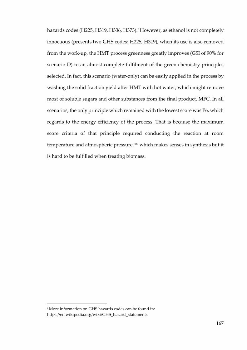
167
hazards codes (H225, H319, H336, H373).f However, as ethanol is not completely
innocuous (presents two GHS codes: H225, H319), when its use is also removed
from the work-up, the HMT process greenness greatly improves (GSI of 90% for
scenario D) to an almost complete fulfilment of the green chemistry principles
selected. In fact, this scenario (water-only) can be easily applied in the process by
washing the solid fraction yield after HMT with hot water, which might remove
most of soluble sugars and other substances from the final product, MFC. In all
scenarios, the only principle which remained with the lowest score was P6, which
regards to the energy efficiency of the process. That is because the maximum
score criteria of that principle required conducting the reaction at room
temperature and atmospheric pressure,307 which makes senses in synthesis but it
is hard to be fulfilled when treating biomass.
f More information on GHS hazards codes can be found in:
https://en.wikipedia.org/wiki/GHS_hazard_statements


169
Chapter 4
4 CONCLUSIONS


171
4.1 Regarding the Obtained Results
As presented in the introduction (Chapter 1), few prior works have been
undertaken on the design of scalable, microwave-based approaches for the
valorisation of orange peel waste.49,126,127 However, these studies neither
considered a fully-integrated (“zero-waste”) process nor were done with in-
depth research. In this work, a new approach based on acid-free hydrothermal
microwave treatment was designed, with focus on the valorisation of the orange
peel cellulosic residue. This valorisation approach resulted in the production of
MFC, a state-of-the-art nanomaterial, besides other valuable biomolecules
extracted from the hydrolysate (pectin, lignin, sugars and other small molecules).
MFC, in particular, was successfully characterised as a nanostructure material
with outstanding physicochemical properties, such as hydrogel formation at low
concentrations. MFC hydrogels presented competitive performance against
conventional rheology modifiers for food and cosmetic applications, as well as
the ability to form strong flexible films, which can find applications in cutting-
edge areas, such as regenerative medicine or flexible electronics. Residual pectin
remaining in DOPR was concomitantly extracted with MFC (but from the
hydrolysate) up to 160 °C. According to its NMR and TGA characterisation, it
presented some degradation of the “hairy” regions (arabinans) above 140 °C,
however, this did not affect its gel formation. Lignin microparticles were
successfully isolated from the hydrolysates generated from high-temperature
HMT experiments (180–220 °C), where several characterisation techniques
confirmed their lignin-like composition and core-shell structure. These lignin
particles can be applied, for instance, as dispersion stabilisers (Pickering
particles), antioxidants, or in composite formulations.297,314 Sugars were the most

172
abundant fraction of soluble molecules identified in the hydrolysates with
important economic value as bioresource, since by means of synthesis or
biotechnology they can be converted into several platform molecules, bio-based
polymers, biofuels and biomaterials.34,39,42
In summary, the hydrothermal microwave treatment applied to the production
of MFC was comparably more energy-efficient than using conventional-heating.
But since current commercial scale of microwave reactors are not optimised for
energy efficiency and scalability,130 the energy consumption values found were
much higher than it would be in an industrial-scale. Also, microwave-heating
presented lower E-factor values than conventional-heating treatment, meaning,
less environmental impact of generated waste per mass of product (MFC). The
overall greenness of the HMT process was found to be higher than that of a
conventional process used in MFC manufacturing, however it could be further
improved by removing the solvent wash steps, which are the main source of
human and environment hazards derived from the HMT process.
In contrast to previous works on this matter,49,126,127 this thesis expands the acid-
free hydrothermal microwave treatment of orange peel waste by including the
valorisation of the overlooked cellulosic residue produced after pectin extraction.
This novel approach offers a more sustainable, scalable and fully-integrated
orange peel biorefinery model, where all by-products are transformed into
valuable materials and biomolecules. This zero-waste biorefinery model is also in
line with the concept of circular-bioeconomy to its fullness, due to increased
circularity of the bio-based resources and products within the economy and the
reduction of waste generation. Another important aspect of this biorefinery

173
model is its feedstock-insensitivity, meaning that it can be applied to other
lignocellulosic biomass besides orange/citrus peel. This study has also greatly
contributed to the nanocellulose research field by presenting a greener and
cleaner alternative methodology for MFC production, which currently is driven
by expensive and not-as-green approaches.1,99,312
4.2 Limitations and Future Work
Although this work was carried out thoroughly, a few limitations were identified
with the purpose to direct and motivate future work.
4.2.1 Regarding MFC characterisation and application
Although a proximate composition analysis of the DOPR and MFC samples was
carried out (Table 3.1), this was based on mixture of indirect data from
instrumental techniques such as TGA, ICP-OES and CHN, which can give a good
approximation of the molecular composition of the material but not as accurate
as it would be using conventional wet chemistry techniques. Therefore, in future
work, proximate composition and analysis should also be carried out by
recommended methodologies, such as the proximate detergent method249 and
other consecutive biomass fractionation methods.315–317 That should also give
clearer separation of biomolecules like pectin and hemicellulose, which cannot
be easily differentiated by TGA for instance.
The assessment of the SEM images of the MFC was slightly affected by the
cellulose fibrils hornification caused mainly by air or oven drying of the sample
prior imaging. Hornification causes the aggregation of the fibrils, which
complicates the dimension measurements of individuals and can alter the
original porous structure of the material. Therefore, for better assessment and

174
accuracy of SEM images, freeze-drying the sample, instead of over or air-drying,
prior to its imaging is recommended. As shown in (Appendix V), the structure
of MFC is better preserved when lyophilised. The concentration of the
suspension should also be kept to a minimum (0.05–0.2%) to avoid overlapping
and aggregation of the fibrils during drying. While TEM is the best available
technique to identify and classify a nanocellulose material as CNF, MFC or
CNC,174,217 other complementary techniques such as (ultra)centrifugation81–83,
mechanical fractionation84 and foam filtration85 should also be explored for the
fractionation of mixed nanocellulose materials (eg. separation of CNF from MFC).
The porous structure of MFC (surface area, pore volume and pore area) analysed
by means of N2 physisorption porosimetry presented some limitations due to the
sample preparation, i.e, the sample had to be dried before the analysis, which
most probably led to hornification, hence the results were not precise. Hence, an
alternative porosimetry method, such as thermoporosimetry (DSC), radiation
scattering and Congo red dye adsorption, that do not require the prior drying of
the sample should be considered in the future.237,240,243
Due to equipment and time limitations, other important characterisation
analyses of MFC, such as surface charge and mechanical properties, were not
investigated in this work, but it is highly recommended for future work, since
these are important properties regarding MFC performance in many
applications, such as dispersions and emulsions stabilizer, composites,
packaging, electronics, etc.77,258
Regarding MFC hydrogels, additional work can be done on its rheological
characterisation, including flow curves (determines the viscosity of the sample at

175
varied shear rates), temperature sweep and structure recovery test (to determine
the rate and extent of viscosity recovery of the sample after shear).266 Moreover,
other application tests should be carried out to test MFC performance in a “real”
product. For example, initial food and cosmetic formulation tests and
antimicrobial activity tests for medical applications.318,319
Although physicochemical analysis and application tests of the MFC films were
beyond the scope of this thesis, the study of its oxygen and other gases barrier
properties, water retention capacity, porosimetry, mechanical properties,
antimicrobial activity, packaging and biomedical applications (i.e. the potential
use of MFC as scaffold for wound dressings) should be explored.
4.2.2 Regarding hydrolysate valorisation
Several valuable products initially identified and extracted from the hydrolysate
in this work can be further characterised and explored for potential applications.
For instance, the GPC analysis of the pectin will add valuable information
regarding the implications of the process temperature (or other parameters) in its
molecular weight, while further testing its gel properties and performance can
give some indication of its potential use in food formulations. Further important
characterisation of lignin microparticles includes GPC, DLS (for particle size),
DSC (thermostability), antioxidant and antimicrobial activity tests. Also,
exploring the performance of lignin microparticles as stabilizer in emulsions and
dispersions, as well as its use in composite formulations (as functional filler,
antimicrobial/antioxidant/hydrophobic agent) is recommended. Lastly, new
research opportunities could be explored by an in-depth analysis of the sugars
and small molecules present in the hydrolysate by LC-MS and GC-MS, as well as

176
the potential of using the extracted sugars in biotechnology for the production of
platform molecules or biofuels (eg. bioethanol).
4.2.3 Regarding the HMT process
Despite the approach presented in this thesis greatly improving and extending
the technical, environmental and economic aspects of previously studied
microwave-based orange peel biorefinery models, there is still room for
improvement.
Starting with the pre-treatment of the feedstock, at lab scale, the biomass should
not be dried (specially oven-dried) prior to any treatment to avoid hornification
of the fibres. Also, particle size should be kept to a minimum (ideally <1 mm) for
better diffusion and extraction of the biomolecules during the microwave
treatment.
Regarding treatment of the feedstock, before the HMT, the extraction of the
essential oil (or d-limonene) by microwave-assisted distillation56 is
recommended, unless the feedstock is coming from an industrial plant which has
already extracted the essential oil as part of their process. That will mimic the
process used in industry but using a cleaner technology (microwave) and should
also reduce the amount of degradation products originating from the presence of
oil residues during the subsequent hydrothermal microwave treatment of orange
peel. The separation of the oil will also add value to the process and its full
characterisation will greatly contribute to the advance of citrus waste valorisation
research. Another step which may be incorporated in the biorefinery model is the
extraction of pigments from orange peel (eg. carotenoids). That could be done by
solvent extraction (Soxhlet or microwave-assisted), however, as the use of

177
solvents like ethanol and acetone has a great impact in the total greenness of the
process (as seen in Section 3.1.4), an organic solvent-free extraction could be
carried out by means of supercritical CO2 for instance, which is a green scalable
technology able to extract less polar compound from biomass feedstocks.111,320 An
integrated pectin and MFC extraction at 120 °C should be carried out in one step
instead of two (as done in this thesis). That should be a better approach regarding
scalability of the process and energy efficiency. In a batch system, increasing
residence time of the sludge in the microwave reactor or/and performing cyclic
re-extractions with new solvent should maximize pectin and sugars extraction
while keeping the cellulosic residue “cleaner”. The extraction temperature of 120
°C is recommend because it: allows the reaction to reach hydrothermal conditions
(autohydrolysis), which might not be achieved at lower temperatures, while
reducing formation of degradation products (such as pseudo-lignin); gives the
best yields for MFC and pectin making the process more profitable; keeps pectin
structure intact with high DE and excellent gel formation and produces an MFC
with most suitable properties for posterior applications (light colour, high WHC,
excellent hydrogel formation with promising rheology behaviour and ability to
form semi-transparent, flexible films).
Regarding the work-up steps for the products isolation (washing and drying), for
MFC, considering that oil, pigments, pectin, sugars and other soluble molecules
has been extracted from the cellulosic matrix, instead of using solvent washes
(which is a major environmental drawback of the process), a better and greener
approach would be repeatedly wash the solid cellulosic residue with hot water
until complete wash of all solubles or using a more reproducible and robust
method, such as membrane ultrafiltration system (also known as tangential flow

178
filtration or cross-flow filtration)41,321, which is a promising green scalable
technology suitable for aqueous systems.120 Finally, for a better performance of
MFC into dispersions and other formulations, the hornification of the cellulose
fibres should be avoided. For that, instead of air- or oven-drying the material
after its isolation and purification, a better drying method would be
lyophilisation (freeze-drying), which should reduce hornification effects,
maintain the porous structure of the material as good as prior drying and
improve its dispersibility in water or other liquids. For the hydrolysate work-up,
cross-flow filtration should be able to successfully separate high-Mw retentate
(pectin) from low-Mw solubles (sugars, oligomers and other small molecules)
and freeze-drying would also be recommended as drying method. Following
these guidelines, a more integrated, greener and efficient biorefinery model for
the orange peel waste valorisation can be designed (Figure 4.1).

179
4.3 Final Remarks
In a broader context, while food waste is still considered an environmental
burden in many countries, due to the lack of incentive from the government body
to support research and technology advancements towards food
waste/agroindustrial biomass valorisation for chemicals and materials, as well as
the lack of technology & knowledge transfer and unviable operational costs,
microwave technology applied to the valorisation of food waste biomass can
bring innumerable benefits for the local economy, environment and scientific
development. Investing in a local microwave-based biorefinery for processing
food waste biomass can drastically reduce operational and logistical costs while
promoting income for food producers and local community, especially in
CITRUS PEEL WASTE
ScCO2 Extraction
Microwave Hydrodistillation
Hydrothermal Microwave Treatment
Solid Residue
Hot Water Wash
Lyophilisation
MFC
Hydrolysate
Cross-flow Filtration
Retentate
PECTIN PROTEINS
Permeate
SUGARS
PIGMENTS
ESSENTIAL OIL
Figure 4.1: Proposed model for a zero-waste orange peel biorefinery generating five high-value
products. Original in colour.

180
developing nations like Brazil, in which the economy is highly dependent on
agriculture. Furthermore, by using an acid-free, water-based process to produce
a high-tech product such as MFC makes the process very competitive and cost-
effective. This approach complies with several of the Sustainable Development
Goals by helping reduce poverty & inequality, creating new job opportunities,
promoting the sustainable use of resources & responsible innovation, reducing
environment & climate impact and promoting circular bioeconomy.

181
REFERENCES
1 Q. Li, S. McGinnis, C. Sydnor, A. Wong and S. Renneckar, ACS Sustain.
Chem. Eng., 2013, 1, 919–928.
2 United Nations, in Climate Change 2013 - The Physical Science Basis, ed.
Intergovernmental Panel on Climate Change, Cambridge University Press,
Cambridge, 2015, pp. 1–30.
3 OECD, Material Resources, Productivity and the Environment,
https://goo.gl/tRhD3z, (accessed 4 April 2018).
4 H. Corvellec, New directions for management and organization studies on
waste, https://bit.ly/2H7WHnO, (accessed 9 November 2018).
5 Plastic Oceans Foundation, The facts, https://bit.ly/2pLpExi, (accessed 17
January 2018).
6 FAO and OECD, OECD-FAO Agricultural Outlook 2015,
https://bit.ly/2BUyJsE, (accessed 9 November 2018).
7 U.S. Energy Information Administration, International Energy Outlook
2017, www.eia.gov/ieo, (accessed 9 January 2018).
8 J. B. Binder and R. T. Raines, J. Am. Chem. Soc., 2009, 131, 1979–1985.
9 Our World in Data (University of Oxford), How long before we run out of
fossil fuels? - Our World in Data, https://bit.ly/2H5pDN3, (accessed 12
January 2018).
10 BP, BP Statistical Review of World Energy 2016,
https://on.bp.com/2VwB3O1, (accessed 12 January 2018).
11 United Nations, Adoption of the Paris Agreement, https://bit.ly/1YbayHO,
(accessed 9 November 2018).
12 C. McGlade and P. Ekins, Nature, 2015, 517, 187–190.
13 Carbon Tracker, Unburnable Carbon 2013: Wasted capital and stranded
assets, https://bit.ly/2deTQMB, (accessed 12 January 2018).
14 IPCC, Special Report on Global Warming of 1.5 oC, https://bit.ly/2pA6aKo,
(accessed 17 October 2018).
15 CICERO, Carbon budget for dummies, https://bit.ly/2tFld7P, (accessed 12
January 2018).

182
16 A. S. Matharu, E. M. de Melo and J. A. Houghton, Bioresour. Technol., 2016,
215, 123–130.
17 S. Liu, Biotechnol. Adv., 2010, 28, 563–582.
18 United Nations, Transforming Our World: The 2030 Agenda for
Sustainable Development, sustainabledevelopment.un.org, (accessed 9
November 2018).
19 FAO, Food wastage footprint. Impacts on natural resources - Summary
Report, https://bit.ly/1kMi2QN, (accessed 9 November 2018).
20 FAO, IFAD, UNICEF, WFP and WHO, The State of Food Security and
Nutrition in the World 2017, https://bit.ly/2jubGOu, (accessed 12 March
2018).
21 D. J. Garcia and F. You, Comput. Chem. Eng., 2016, 91, 49–67.
22 FAO, Global initiative on food loss and food waste reduction,
http://www.fao.org/save-food/en/, (accessed 22 March 2018).
23 M. Bond, T. Meacham, R. Bhunnoo and T. G. Benton, Food waste within
global food systems, www.foodsecurity.ac.uk, (accessed 9 November
2018).
24 E. Vandamme, T. Anthonis and S. Dobbelaere, Industrial Biomass: Source
of Chemicals, Materials, and Energy!
25 A. S. Matharu, E. M. de Melo and J. A. Houghton, in Routledge Handbook of
the Resource Nexus, eds. R. Bleischwitz, H. Hoff, C. Spataru, E. van der Voet
and S. D. VanDeveer, Routledge, 2017, pp. 457–467.
26 B. Bilska, M. Wrzosek, D. Kołożyn-Krajewska and K. Krajewski, Waste
Manag., 2016, 52, 269–277.
27 J. Hargreaves, I. Pulford, M. Balakrishnan and V. Batra, Conversion of Large
Scale Wastes into Value-added Products, CRC Press, 2013.
28 M. Z. Jacobson, J. Geophys. Res. Atmos., 2014, 119, 8980–9002.
29 C. O. Tuck, E. Pérez, I. T. Horváth, R. a Sheldon and M. Poliakoff, Science,
2012, 337, 695–9.
30 E. Scott, F. Peter and J. Sanders, Appl. Microbiol. Biotechnol., 2007, 75, 751–
762.
31 M. Carus and L. Dammer, The " Circular Bioeconomy " – Concepts,

183
Opportunities and Limitations, www.bio-based.eu/nova-papers, (accessed
15 November 2018).
32 MIT, The dirty secret of biomass waste, https://bit.ly/2Tm8zc1, (accessed 9
November 2018).
33 Q. Xu, L.-L. Chen, X. Ruan, D. Chen, A. Zhu, C. Chen, D. Bertrand, W.-B.
Jiao, B.-H. Hao, M. P. Lyon, J. Chen, S. Gao, F. Xing, H. Lan, J.-W. Chang,
X. Ge, Y. Lei, Q. Hu, Y. Miao, L. Wang, S. Xiao, M. K. Biswas, W. Zeng, F.
Guo, H. Cao, X. Yang, X.-W. Xu, Y.-J. Cheng, J. Xu, J.-H. Liu, O. J. Luo, Z.
Tang, W.-W. Guo, H. Kuang, H.-Y. Zhang, M. L. Roose, N. Nagarajan, X.-
X. Deng and Y. Ruan, Nat. Genet., 2013, 45, 59–66.
34 P. Putnik, D. Bursać Kovačević, A. Režek Jambrak, F. Barba, G. Cravotto,
A. Binello, J. Lorenzo and A. Shpigelman, Molecules, 2017, 22, 680–703.
35 FAO, Citrus Fruit Fresh and Processed Statistical Bulletin 2016,
https://bit.ly/2tGIpSS, (accessed 9 November 2018).
36 FAO, FAO Statistics, http://faostat.fao.org, (accessed 9 November 2018).
37 C. Chen, Pigments in fruits and vegetables: Genomics and dietetics, Springer,
Lake Alfred, USA, 2015.
38 U. Ringblom, The Orange Book, Tetra Pak Processing Systems, Lund,
Sweden, 3rd edn., 2017.
39 D. Mamma and P. Christakopoulos, Waste and Biomass Valorization, 2014, 5,
529–549.
40 I. John, K. Muthukumar and A. Arunagiri, Int. J. Green Energy, 2017, 14,
599–612.
41 J. A. Houghton, PhD Thesis, University of York, 2017.
42 C. S. K. Lin, L. A. Pfaltzgraff, L. Herrero-Davila, E. B. Mubofu, S.
Abderrahim, J. H. Clark, A. A. Koutinas, N. Kopsahelis, K. Stamatelatou,
F. Dickson, S. Thankappan, Z. Mohamed, R. Brocklesby and R. Luque,
Energy Environ. Sci., 2013, 6, 426–464.
43 J. Á. S. López, Q. Li and I. P. Thompson, Crit. Rev. Biotechnol., 2010, 30, 63–
69.
44 V. Heuzé, G. Tran, P. Hassoun and F. Lebas, Feedpedia - Citrus pulp, fresh,
https://www.feedipedia.org/node/679, (accessed 15 November 2018).

184
45 V. Negro, G. Mancini, B. Ruggeri and D. Fino, Bioresour. Technol., 2016, 214,
806–815.
46 R. Wikandari, H. Nguyen, R. Millati, C. Niklasson and M. J. Taherzadeh,
Biomed Res. Int., 2015, 2015, 1–6.
47 C. M. Santos, J. Dweck, R. S. Viotto, A. H. Rosa and L. C. de Morais,
Bioresour. Technol., 2015, 196, 469–479.
48 L. Aguiar, F. Márquez-Montesinos, A. Gonzalo, J. L. Sánchez and J. Arauzo,
J. Anal. Appl. Pyrolysis, 2008, 83, 124–130.
49 L. A. Pfaltzgraff, PhD Thesis, University of York, 2014.
50 Brazil, Política Nacional de Resíduos Sólidos, https://bit.ly/2J0A7MJ,
(accessed 14 June 2018).
51 T. L. H. Treuer, J. J. Choi, D. H. Janzen, W. Hallwachs, D. Peréz-Aviles, A.
P. Dobson, J. S. Powers, L. C. Shanks, L. K. Werden and D. S. Wilcove,
Restor. Ecol., 2018, 26, 275–283.
52 A. S. Matharu, E. M. de Melo and J. A. Houghton, in Waste biorefinery:
potential and perspectives, eds. T. Bhaskar, A. Pandey, S. V. Mohan, D. J. Lee
and S. K. Khanal, Elsevier, 1st edn., 2018, pp. 219–233.
53 L. A. Pfaltzgraff, M. De bruyn, E. C. Cooper, V. Budarin and J. H. Clark,
Green Chem., 2013, 15, 307–314.
54 F. R. Marín, C. Soler-Rivas, O. Benavente-García, J. Castillo and J. a. Pérez-
Alvarez, Food Chem., 2007, 100, 736–741.
55 G. Dugo and A. Di Giacomo, Citrus: The Genus Citrus, Taylor & Francis
Group, 1st edn., 2002.
56 J. Bustamante, S. van Stempvoort, M. García-Gallarreta, J. A. Houghton, H.
K. Briers, V. L. Budarin, A. S. Matharu and J. H. Clark, J. Clean. Prod., 2016,
137, 598–605.
57 Intracen, Price information of conventional essential oils,
https://bit.ly/2VsLwdg, (accessed 15 November 2018).
58 R. Ciriminna, N. Chavarría-Hernández, A. Inés Rodríguez Hernández and
M. Pagliaro, Biofuels, Bioprod. Biorefining, 2015, 9, 368–377.
59 J. Harholt, A. Suttangkakul and H. Vibe Scheller, Plant Physiol., 2010, 153,
384–395.

185
60 Global Info Research, Global Pectin Market by Manufacturers, Regions,
Type and Application, Forecast to 2021, https://bit.ly/2VrN0nM, (accessed
15 November 2018).
61 R. Ciriminna, A. Fidalgo, R. Delisi, A. Tamburino, D. Carnaroglio, G.
Cravotto, L. M. Ilharco and M. Pagliaro, ACS Omega, 2017, 2, 7991–7995.
62 R. Ciriminna, A. Fidalgo, R. Delisi, I. M. Ilharco and M. Pagliaro, Agro Food
Ind. Hi Tech, 2016, 27(5), 17–20.
63 B. H. Davison, J. Parks, M. F. Davis and B. S. Donohoe, in Aqueous
Pretreatment of Plant Biomass for Biological and Chemical Conversion to Fuels
and Chemicals, John Wiley & Sons, Ltd, Chichester, UK, 2013, pp. 23–38.
64 G. Costa and I. Plazanet, Adv. Biol. Chem., 2016, 6, 70–105.
65 M. A. C. M. Haniffa, Y. Ching, L. Abdullah, S. Poh and C. Chuah, Polymers
(Basel)., 2016, 8, 246.
66 E. F. Lessa, M. S. Gularte, E. S. Garcia and A. R. Fajardo, Carbohydr. Polym.,
2017, 157, 660–668.
67 P. D. Pathak, S. A. Mandavgane and B. D. Kulkarni, Rev. Chem. Eng., 2015,
31, 361–381.
68 O. Pezoti, A. L. Cazetta, K. C. Bedin, L. S. Souza, R. P. Souza, S. R. Melo and
V. C. Almeida, Chem. Eng. J., 2016, 283, 1305–1314.
69 USPTO, US20080193590, 2008.
70 USPTO, US 7094317 B2, 2006.
71 USPTO, US 2014/0356463 A1, 2014.
72 USPTO, WO2001017376A1, 2000.
73 USPTO, WO1994027451 A1, 1994.
74 Internet, Nanocellulose for tires: something new in performance and
sustainability : Biofuels Digest, https://goo.gl/47VeNO, (accessed 9 March
2017).
75 M. Mariano and A. Dufresne, in Nanocelluloses: Their Preparation, Properties,
and Applications - ACS Symposium Series, American Chemical Society,
Washington, USA, 2017, pp. 203–225.
76 H. Kargarzadeh, M. Ioelovich, I. Ahmad, S. Thomas and A. Dufresne, in

186
Handbook of Nanocellulose and Cellulose Nanocomposites, Wiley-VCH Verlag
GmbH & Co. KGaA, Weinheim, Germany, 2017, pp. 1–49.
77 D. Klemm, F. Kramer, S. Moritz, T. Lindström, M. Ankerfors, D. Gray and
A. Dorris, Angew. Chemie Int. Ed., 2011, 50, 5438–5466.
78 W. Y. Hamad, Cellulose Nanocrystals: Properties, production and applications,
John Wiley & Sons, Chichester, UK, 2017.
79 G. Chinga-Carrasco, Nanoscale Res. Lett., 2011, 6, 417.
80 N. Lavoine, I. Desloges, A. Dufresne and J. Bras, Carbohydr. Polym., 2012,
90, 735–764.
81 S. Alila, I. Besbes, M. R. Vilar, P. Mutjé and S. Boufi, Ind. Crops Prod., 2013,
41, 250–259.
82 R. Salminen, M. Reza, T. Pääkkönen, J. Peyre and E. Kontturi, Cellulose,
2017, 24, 1657–1667.
83 H. Bian, L. Chen, R. Gleisner, H. Dai and J. Y. Zhu, Green Chem., 2017, 19,
3370–3379.
84 A. Tanaka, V. Seppanen, J. Houni, A. Sneck and P. Pirkonen, Nord. Pulp
Pap. Res. J., 2012, 27, 689–694.
85 A. Tanaka, T. Hjelt, A. Sneck and A. Korpela, Sep. Sci. Technol., 2012, 47,
1771–1776.
86 A. Dufresne, Philos. Trans. R. Soc. A Math. Phys. Eng. Sci., 2018, 376,
20170040.
87 USPTO, US20150158955 A1, 2015.
88 S. H. Osong, S. Norgren and P. Engstrand, Cellulose, 2016, 23, 93–123.
89 Internet, Nanocellulose State of the Industry, https://goo.gl/Tzz2WV,
(accessed 14 November 2018).
90 USPTO, US9187865 B2, 2015.
91 Borregaard, Microfibrillated Cellulose at a glance, https://goo.gl/EJHTo9,
(accessed 18 September 2017).
92 A. Dufresne, Mater. Today, 2013, 16, 220–227.
93 Markets and Markets, Global Nanocellulose Market - Forecast until 2019,

187
https://bit.ly/2EBo6wr, (accessed 11 November 2018).
94 G. Ström, C. Öhgren and M. Ankerfors, Nanocellulose as an additive in
foodstuff, https://bit.ly/2Vpl1oT, (accessed 15 November 2018).
95 C. Gómez H., A. Serpa, J. Velásquez-Cock, P. Gañán, C. Castro, L. Vélez
and R. Zuluaga, Food Hydrocoll., 2016, 57, 178–186.
96 T. Abitbol, A. Rivkin, Y. Cao, Y. Nevo, E. Abraham, T. Ben-Shalom, S.
Lapidot and O. Shoseyov, Curr. Opin. Biotechnol., 2016, 39, 76–88.
97 N. Lavoine and L. Bergström, J. Mater. Chem. A, 2017, 5, 16105–16117.
98 H. M. C. Azeredo, M. F. Rosa and L. H. C. Mattoso, Ind. Crops Prod., 2017,
97, 664–671.
99 C. A. de Assis, C. Houtman, R. Phillips, E. M. T. Bilek, O. J. Rojas, L. Pal,
M. S. Peresin, H. Jameel and R. Gonzalez, Biofuels, Bioprod. Biorefining, 2017,
11, 682–700.
100 Internet, Nanocellulose prices, https://www.celluloselab.com/, (accessed
21 September 2017).
101 Y. Mälkki, MOJ Food Process. Technol., 2017, 4, 1–3.
102 K. Nelson, T. Retsina, M. Iakovlev, A. van Heiningen, Y. Deng, J. A. Shatkin
and A. Mulyadi, in Materials Research for Manufacturing - An Industrial
Perspective of Turning Materials into New Products, eds. L. D. Madsen and E.
B. Svedberg, Springer, 2016, pp. 267–302.
103 Fraunhofer, Agri and food waste valorisation co-ops based on flexible
multi-feedstocks biorefinery processing technologies for new high added
value applications., https://bit.ly/2SwG8Ur, (accessed 14 December 2017).
104 M. Mariño, L. Lopes da Silva, N. Durán and L. Tasic, Molecules, 2015, 20,
5908–5923.
105 A. García, A. Gandini, J. Labidi, N. Belgacem and J. Bras, Ind. Crops Prod.,
2016, 93, 26–38.
106 M. Boukroufa, C. Boutekedjiret, L. Petigny, N. Rakotomanomana and F.
Chemat, Ultrason. Sonochem., 2014, 24, 72–79.
107 A. M. Balu, V. Budarin, P. S. Shuttleworth, L. A. Pfaltzgraff, K. Waldron, R.
Luque and J. H. Clark, ChemSusChem, 2012, 5, 1694–1697.
108 J. Tsukamoto, N. Durán and L. Tasic, J. Braz. Chem. Soc., 2013, 24, 1537–

188
1543.
109 B. Satari, J. Palhed, K. Karimi, M. Lundin, M. J. Taherzadeh and A. Zamani,
BioResources, 2017, 12, 1706–1722.
110 J. S. Van Dyk, R. Gama, D. Morrison, S. Swart and B. I. Pletschke, Renew.
Sustain. Energy Rev., 2013, 26, 521–531.
111 S. R. Shirsath, S. H. Sonawane and P. R. Gogate, Chem. Eng. Process. Process
Intensif., 2012, 53, 10–23.
112 K. Kaderides, A. M. Goula and K. G. Adamopoulos, Innov. Food Sci. Emerg.
Technol., 2015, 31, 204–215.
113 I. John, P. Yaragarla, P. Muthaiah, K. Ponnusamy and A. Appusamy,
Resour. Technol., 2017, 3, 429–433.
114 USPTO, US9169523B2, 2015.
115 SAIREM, Industrial Microwave Systems & Components
Manufacturing - SAIREM, https://www.sairem.com/, (accessed 22 June
2018).
116 AMT, Advanced Microwave Technologies, https://bit.ly/2NwnZFi,
(accessed 22 June 2018).
117 IDCO, IDCO - Microwave Technology, http://www.idco-france.com/,
(accessed 22 June 2018).
118 Y. Li, A.-S. Fabiano-Tixier, M. Abert-Vian and F. Chemat, in Microwave-
assisted Extraction for Bioactive Compounds: Theory and Practice, eds. F.
Chemat and G. Cravotto, Springer US, Boston, MA, 2013, pp. 103–125.
119 E. Destandau, T. Michel and C. Elfakir, in Natural Product Extraction:
Principles and Applications, eds. M. A. Rostagno and J. M. Prado, The Royal
Society of Chemistry, 2013, pp. 113–156.
120 N. Flórez, E. Conde and H. Domínguez, J. Chem. Technol. Biotechnol., 2015,
90, 590–607.
121 C. O. Kappe, Angew. Chemie Int. Ed., 2004, 43, 6250–6284.
122 C. O. Kappe, B. Pieber and D. Dallinger, Angew. Chemie Int. Ed., 2013, 52,
1088–1094.
123 S. Tsubaki and J.-I. Azum, in Advances in Induction and Microwave Heating
of Mineral and Organic Materials, InTech, 2011, pp. 697–722.

189
124 D. J. Macquarrie, J. H. Clark and E. Fitzpatrick, Biofuels, Bioprod. Biorefining,
2012, 6, 549–560.
125 J. González-Rivera, A. Spepi, C. Ferrari, C. Duce, I. Longo, D. Falconieri, A.
Piras and M. R. Tinè, Green Chem., 2016, 18, 6482–6492.
126 USPTO, US 2015/0065698 A1, 2015.
127 A. Bagaria, MRes Thesis, University of York, 2014.
128 P. T. Anastas and J. C. Warner, Green Chemistry: Theory and Practice, Oxford
University Press, Incorporated, 1998.
129 D. Kim, S. K. Seol and W. S. Chang, Korean J. Chem. Eng., 2016, 33, 527–531.
130 R. Luque, J. A. Menéndez, A. Arenillas and J. Cot, Energy Environ. Sci., 2012,
5, 5481–5488.
131 J. D. Moseley and C. O. Kappe, Green Chem., 2011, 13, 794–806.
132 J. D. Moseley and E. K. Woodman, Energy & Fuels, 2009, 23, 5438–5447.
133 E. M. de Melo, J. H. Clark and A. S. Matharu, Green Chem., 2017, 19, 3408–
3417.
134 M. J. Serapiglia, K. D. Cameron, A. J. Stipanovic and L. B. Smart, BioEnergy
Res., 2009, 2, 1–9.
135 M. J. Serapiglia, K. D. Cameron, A. J. Stipanovic and L. B. Smart, Appl.
Biochem. Biotechnol., 2008, 145, 3–11.
136 T.-Q. Yuan, F. Xu, J. He and R.-C. Sun, Biotechnol. Adv., 2010, 28, 583–593.
137 K. Werner, L. Pommer and M. Broström, J. Anal. Appl. Pyrolysis, 2014, 110,
130–137.
138 H. Zhu, Z. Fang, C. Preston, Y. Li and L. Hu, Energy Environ. Sci., 2014, 7,
269–287.
139 A. Sluiter, B. Hames, R. Ruiz, C. Scarlata, J. Sluiter, D. Templeton and D.
Crocker, Lab. Anal. Proced., 2012, 1, 1–15.
140 A. M. Magomya, D. Kubmarawa, J. A. Ndahi and G. G. Yebpella, Int. J. Sci.
Technol. Res., 2014, 3, 68–72.
141 J. Zhang, Y. Hu and Y. Li, Gel Chemistry, Springer Singapore, Singapore,
2018, vol. 96.

190
142 S. R. Raghavan and B. H. Cipriano, in Molecular Gels: Materials with Self-
Assembled Fibrillar Networks, Springer-Verlag, Berlin/Heidelberg, 2005, pp.
241–252.
143 S. Park, J. O. Baker, M. E. Himmel, P. A. Parilla and D. K. Johnson,
Biotechnol. Biofuels, 2010, 3, 3–10.
144 L. Segal, J. J. Creely, A. E. Martin and C. M. Conrad, Text. Res. J., 1959, 29,
786–794.
145 A. K. Pathan, J. Bond and R. E. Gaskin, Mater. Today, 2010, 12, 32–43.
146 S. Lowell, J. E. Shields, M. A. Thomas and M. Thommes, Characterization of
Porous Solids and Powders: Surface Area, Pore Size and Density, Springer
Netherlands, Dordrecht, 2004, vol. 16.
147 N. F. Mat Zain, S. M. Yusop and I. Ahmad, J. Nutr. Food Sci., 2014, 05, 10–
13.
148 R. Berggren, F. Berthold, E. Sjöholm and M. Lindström, J. Appl. Polym. Sci.,
2003, 88, 1170–1179.
149 W. Wang and J.-H. Liu, Gene, 2015, 555, 421–429.
150 H.-D. Belitz, W. Grosch and P. Schieberle, Food Chemistry, Springer Berlin
Heidelberg, Berlin, Heidelberg, 2009, vol. 107.
151 G. E. Ravilious and J. M. Jez, Nat. Prod. Rep., 2012, 29, 1138.
152 K. E. M. Hendricks, R. S. Donahoo, P. D. Roberts and M. C. Christman, Am.
J. Plant Sci., 2013, 04, 282–290.
153 E. Rodrigues, I. I. Rockenbach, C. Cataneo, L. V. Gonzaga, E. S. Chaves and
R. Fett, Ciência e Tecnol. Aliment., 2009, 29, 642–645.
154 J. Sidana, V. Saini, S. Dahiya, P. Nain and S. Bala, Int. J. Pharm. Sci. Rev. Res.,
2013, 18, 20–27.
155 Y.-M. Kim, H. W. Lee, S. Kim, C. Watanabe and Y.-K. Park, BioEnergy Res.,
2015, 8, 431–439.
156 F. Hu, S. Jung and A. Ragauskas, Bioresour. Technol., 2012, 117, 7–12.
157 I. Aarum, H. Devle, D. Ekeberg, S. J. Horn and Y. Stenstrøm, ACS Omega,
2018, 3, 4924–4931.
158 S. D. Shinde, X. Meng, R. Kumar and A. J. Ragauskas, Green Chem., 2018,

191
20, 2192–2205.
159 K. Yao, Q. Wu, R. An, W. Meng, M. Ding, B. Li and Y. Yuan, AIChE J., 2018,
64, 1938–1953.
160 P. Sannigrahi, D. H. Kim, S. Jung and A. Ragauskas, Energy Environ. Sci.,
2011, 4, 1306–1310.
161 F. Araya, E. Troncoso, R. T. Mendonça and J. Freer, Biotechnol. Bioeng., 2015,
112, 1783–1791.
162 L. Moghaddam, J. Rencoret, V. R. Maliger, D. W. Rackemann, M. D.
Harrison, A. Gutiérrez, J. C. del Río and W. O. S. Doherty, ACS Sustain.
Chem. Eng., 2017, 5, 4846–4855.
163 L. Zhou, V. Budarin, J. Fan, R. Sloan and D. Macquarrie, ACS Sustain. Chem.
Eng., 2017, 5, 3768–3774.
164 G. van Erven, R. de Visser, D. W. H. Merkx, W. Strolenberg, P. de Gijsel, H.
Gruppen and M. A. Kabel, Anal. Chem., 2017, 89, 10907–10916.
165 A. Duval and M. Lawoko, React. Funct. Polym., 2014, 85, 78–96.
166 M. Carrier, A. Loppinet-Serani, D. Denux, J.-M. Lasnier, F. Ham-Pichavant,
F. Cansell and C. Aymonier, Biomass and Bioenergy, 2011, 35, 298–307.
167 Y. Luo, J. Fan, V. L. Budarin, C. Hu and J. H. Clark, Green Chem., ,
DOI:10.1039/C7GC02300F.
168 S. Sabiha-Hanim and A. Aziatul-Akma, in Polymer Science: Research
Advances, Practical Applications and Educational Aspects, eds. A. Méndez-
Vilas and A. Solano-Martín, Formatex Research Center, Spain, 2016, pp.
404–411.
169 S. Hiasa, S. Iwamoto, T. Endo and Y. Edashige, Ind. Crops Prod., 2014, 62,
280–285.
170 A. T. Quitain, T. Kai, M. Sasaki and M. Goto, Ind. Eng. Chem. Res., 2013, 52,
7940–7946.
171 T. Röder and H. Sixta, Lenzinger Berichte, 2004, 83, 79–83.
172 L.-S. Johansson, T. Tammelin, J. M. Campbell, H. Setälä and M. Österberg,
Soft Matter, 2011, 7, 10917.
173 M. V. Zimmermann, C. Borsoi, A. Lavoratti, M. Zanini, A. J. Zattera and R.
M. Santana, J. Reinf. Plast. Compos., 2016, 35, 628–643.

192
174 M. Kaushik, C. Fraschini, G. Chauve, J.-L. Putaux and A. Moores, in The
Transmission Electron Microscope - Theory and Applications, InTech, 2015.
175 K. Karimi and M. J. Taherzadeh, Bioresour. Technol., 2016, 200, 1008–1018.
176 A. S. Matharu, E. M. de Melo, J. Remón, S. Wang, A. Abdulina and E.
Kontturi, ChemSusChem, 2018, 11, 1344–1353.
177 J. Fan, M. De bruyn, V. L. Budarin, M. J. Gronnow, P. S. Shuttleworth, S.
Breeden, D. J. Macquarrie and J. H. Clark, J. Am. Chem. Soc., 2013, 135,
11728–11731.
178 M. C. Jarvis, Philos. Trans. R. Soc. A Math. Phys. Eng. Sci., 2018, 376,
20170045.
179 I. Usov, G. Nyström, J. Adamcik, S. Handschin, C. Schütz, A. Fall, L.
Bergström and R. Mezzenga, Nat. Commun., 2015, 6, 7564.
180 F. Navarro, PhD Thesis, Virginia Polytechnic Institute and State University,
2010.
181 R. H. Atalla, R. S. Atalla and U. P. Agarwal, in Nanocelluloses: Their
Preparation, Properties, and Applications - ACS Symposium Series, American
Chemical Society, Washington, USA, 2017, vol. 23, pp. 1–18.
182 F. W. Herrick, R. L. Caseiber, J. K. Hamilton and K. R. Sandberg, J. Appl.
Polym. Sci. Appl. Polym. Symp., 1983, 37, 797–813.
183 D. J. Cosgrove, Nat. Rev. Mol. Cell Biol., 2005, 6, 850–861.
184 M. McCann, B. Wells and K. Roberts, J. Cell Sci., 1990, 96, 323–334.
185 N. Billinton and A. W. Knight, Anal. Biochem., 2001, 291, 175–197.
186 J. A. Olmstead, J. H. Zhu and D. G. Gray, Can. J. Chem., 1995, 73, 1955–1959.
187 P. Singh and A. Pandey, Biotechnology for Agro-Industrial Residues
Utilisation, 2009.
188 S. Singh, G. Cheng, N. Sathitsuksanoh, D. Wu, P. Varanasi, A. George, V.
Balan, X. Gao, R. Kumar, B. E. Dale, C. E. Wyman and B. A. Simmons, Front.
Energy Res., 2015, 2, 1–12.
189 T. A. Chimenez, M. H. Gehlen, K. Marabezi and A. A. S. Curvelo, Cellulose,
2014, 21, 653–664.
190 L. Donaldson and A. Vaidya, Sci. Rep., 2017, 7, 1–14.

193
191 V. C. Coletta, C. A. Rezende, F. R. da Conceição, I. Polikarpov and F. E. G.
Guimarães, Biotechnol. Biofuels, 2013, 6, 1–10.
192 H. Wondraczek, A. Kotiaho, P. Fardim and T. Heinze, Carbohydr. Polym.,
2011, 83, 1048–1061.
193 S. Singh, B. A. Simmons and K. P. Vogel, Biotechnol. Bioeng., 2009, 104, 68–
75.
194 J. Zhuang, X. Wang, J. Xu, Z. Wang and M. Qin, Wood Sci. Technol., 2017,
51, 165–174.
195 F. Hu, PhD Thesis, Georgia Institute of Technology, 2014.
196 J. A. Olmstead and D. G. Gray, J. Photochem. Photobiol. A Chem., 1993, 73,
59–65.
197 Y. Wang, Plant Omics, 2012, 5, 508–513.
198 C. Sene, M. C. McCann, R. H. Wilson and R. Grinter, Plant Physiol., 1994,
106, 1623–1631.
199 M.-J. Chen, X.-Q. Zhang, A. Matharu, E. Melo, R.-M. Li, C.-F. Liu and Q.-S.
Shi, ACS Sustain. Chem. Eng., 2017, 5, 7278–7283.
200 F. Lionetto, R. Del Sole, D. Cannoletta, G. Vasapollo and A. Maffezzoli,
Materials (Basel)., 2012, 5, 1910–1922.
201 J. A. Perez-Pimienta, M. G. Lopez-Ortega, J. A. Chavez-Carvayar, P.
Varanasi, V. Stavila, G. Cheng, S. Singh and B. A. Simmons, Biomass and
Bioenergy, 2015, 75, 180–188.
202 J. A. Perez-Pimienta, H. M. Poggi-Varaldo, T. Ponce-Noyola, A. C. Ramos-
Valdivia, J. A. Chavez-Carvayar, V. Stavila and B. A. Simmons, Biomass and
Bioenergy, 2016, 91, 48–55.
203 O. N. Friday and M. M. Muhammad, J. Appl. Sci. Environ. Manag., 2015, 19,
787–792.
204 Y. Pu, B. Hallac and A. J. Ragauskas, in Aqueous Pretreatment of Plant
Biomass for Biological and Chemical Conversion to Fuels and Chemicals, John
Wiley & Sons, Ltd, Chichester, UK, 2013, pp. 369–390.
205 Z. A. Popper, T. J. Bootten, P. J. Harris, L. D. Melton and R. H. Newman,
The Plant Cell Wall, Humana Press, Totowa, NJ, 2011, vol. 715.
206 R. M. S. Ratnayake, I. M. Sims, R. H. Newman and L. D. Melton, J. Agric.

194
Food Chem., 2011, 59, 7186–7193.
207 W. Chen, Q. Li, J. Cao, Y. Liu, J. Li, J. Zhang, S. Luo and H. Yu, Carbohydr.
Polym., 2015, 117, 950–956.
208 H. Halonen, PhD Thesis, Royal Institute of Technology, 2012.
209 M. Bardet, M. F. Foray, J. Bourguignon and P. Krajewski, Magn. Reson.
Chem., 2001, 39, 733–738.
210 M. Dick-Perez, T. Wang, A. Salazar, O. A. Zabotina and M. Hong, Magn.
Reson. Chem., 2012, 50, 539–550.
211 H. Tang, P. S. Belton, A. Ng and P. Ryden, J. Agric. Food Chem., 1999, 47,
510–517.
212 G. D. Love, C. E. Snape and M. C. Jarvis, Phytochemistry, 1998, 49, 1191–
1194.
213 O. D. Bernardinelli, M. A. Lima, C. A. Rezende, I. Polikarpov and E. R.
DeAzevedo, Biotechnol. Biofuels, 2015, 8, 110.
214 S. Xiao, R. Gao, Y. Lu, J. Li and Q. Sun, Carbohydr. Polym., 2015, 119, 202–
209.
215 X. Ouyang, W. Wang, Q. Yuan, S. Li, Q. Zhang and P. Zhao, RSC Adv., 2015,
5, 61650–61656.
216 M. Hajir, R. Graf and W. Tremel, Chem. Commun., 2014, 50, 6534–6536.
217 C. S. Davis, R. J. Moon, S. Ireland, L. Johnston, J. A. Shatkin, K. Nelson, E.
J. Foster, A. M. Forster, M. T. Postek, A. Vladar and J. W. Gilman, in 2014
TAPPI International Conference on Nanotechnology for Renewable Materials
Report, National Institute of Standards and Technology, Gaithersburg, MD,
2015, pp. 1–42.
218 Kathryn Lawson-Wood and Ian Robertson, Decomposition of Calcium
Oxalate Monohydrate using a Hyphenated TG-IR system,
https://bit.ly/2BWtpFh, (accessed 16 September 2017).
219 M. Brebu and C. Vasile, Cellul. Chem. Technol., 2010, 44, 353–363.
220 R. Sánchez Orozco, P. Balderas Hernández, G. Roa Morales, F. Ureña
Núñez, J. Orozco Villafuerte, V. Lugo Lugo, N. Flores Ramírez, C. E.
Barrera Díaz and P. Cajero Vázquez, BioResources, 2014, 9, 1873–1885.
221 A. Potthast, S. Radosta, B. Saake, S. Lebioda, T. Heinze, U. Henniges, A.

195
Isogai, A. Koschella, P. Kosma, T. Rosenau, S. Schiehser, H. Sixta, M. Strlič,
G. Strobin, W. Vorwerg and H. Wetzel, Cellulose, 2015, 22, 1591–1613.
222 J. Oberlerchner, T. Rosenau and A. Potthast, Molecules, 2015, 20, 10313–
10341.
223 B. B. Hallac and A. J. Ragauskas, Biofuels, Bioprod. Biorefining, 2011, 5, 215–
225.
224 V. L. Budarin, J. H. Clark, B. A. Lanigan, P. Shuttleworth and D. J.
Macquarrie, Bioresour. Technol., 2010, 101, 3776–3779.
225 M. Lorenz, S. Sattler, M. Reza, A. Bismarck and E. Kontturi, Faraday
Discuss., 2017, 202, 315–330.
226 Y. Habibi, Chem. Soc. Rev., 2014, 43, 1519–1542.
227 I. Siró and D. Plackett, Cellulose, 2010, 17, 459–494.
228 A. B. Fall, A. Burman and L. Wågberg, Spec. Issue Nanocellulose - Nord. Pulp
Pap. Res. J., 2014, 29, 176–184.
229 O. Ibraheem and B. K. Ndimba, Int. J. Biol. Sci., 2013, 9, 598–612.
230 M. Dashtban, A. Gilbert and P. Fatehi, J. Sci. Technol. For. Prod. Process.,
2012, 2, 44–53.
231 Y. Zhao, H. Lin and S. Wang, Energy Sci. Eng., 2017, 5, 208–216.
232 A. Shafeeq, A. Muhammad, S. Sarfaraz, Z. Akram, H. M. U. Saeed and U.
Farooq, Int. J. Chem. Eng. Appl., 2015, 6, 381–384.
233 J. Nemoto, T. Saito and A. Isogai, ACS Appl. Mater. Interfaces, 2015, 7, 19809–
19815.
234 K. Kekäläinen, PhD Thesis, University of Oulu, 2016.
235 H. Chen, in Biotechnology of Lignocellulose: Theory and Practice, 2014, pp. 1–
511.
236 S. Viamajala, B. S. Donohoe, S. R. Decker, T. B. Vinzant, M. J. Selig, M. E.
Himmel and M. P. Tucker, in Sustainable Biotechnology: Sources of Renewable
Energy, Springer Netherlands, 2010, pp. 1–18.
237 A. Julbe and J. D. F. Ramsay, in Membrane Science and Technology, Elsevier,
1996, vol. 4, pp. 67–118.

196
238 D. Topgaard and O. Söderman, in Magnetic Resonance in Colloid and Interface
Science, Springer Netherlands, Dordrecht, 2002, pp. 631–635.
239 R. G. Munro, Porosity and Specific Surface Area Measurements for Solid
Materials, http://www.ncbi.nlm.nih.gov/pubmed/22544181, (accessed 31
January 2018).
240 L. M. Anovitz and D. R. Cole, Rev. Mineral. Geochemistry, 2015, 80, 61–164.
241 Z. Lu, Z. Su, S. Song, Y. Zhao, S. Ma and M. Zhang, Cellulose, 2018, 25, 619–
629.
242 S. F. Santos, G. H. D. Tonoli, J. E. B. Mejia, J. Fiorelli and H. Savastano Jr,
Mater. Construcción, 2015, 65, e041.
243 K. L. Spence, R. A. Venditti, O. J. Rojas, Y. Habibi and J. J. Pawlak, Cellulose,
2011, 18, 1097–1111.
244 A. Borisova, M. De Bruyn, V. L. Budarin, P. S. Shuttleworth, J. R. Dodson,
M. L. Segatto and J. H. Clark, Macromol. Rapid Commun., 2015, 36, 774–779.
245 N. Mahfoudhi and S. Boufi, Cellulose, 2017, 24, 1171–1197.
246 S. S. Cho and M. L. Dreher, Handbook of dietary fiber, Taylor & Francis, New
York, NY, 2001, vol. 113.
247 R. G. M. van der Sman, E. Paudel, A. Voda and S. Khalloufi, Food Res. Int.,
2013, 54, 804–811.
248 Y. Qin, X. Qiu and J. Y. Zhu, Sci. Rep., 2016, 6, 1–12.
249 P. J. Van Soest, in Nutritional Ecology of the Ruminant, Cornell University
Press, 2nd., 1994, pp. 140–155.
250 N. Lin, J. Huang and A. Dufresne, Nanoscale, 2012, 4, 3274–3294.
251 R. J. Moon, A. Martini, J. Nairn, J. Simonsen and J. Youngblood, Chem. Soc.
Rev., 2011, 40, 3941.
252 M. Bulota, B. Maasdam and S. Tiekstra, Breakthrough technologies,
https://bit.ly/2NxDsF5, (accessed 21 September 2018).
253 K. J. De France, T. Hoare and E. D. Cranston, Chem. Mater., 2017, 29, 4609–
4631.
254 H. Dong, J. F. Snyder, D. T. Tran and J. L. Leadore, Carbohydr. Polym., 2013,
95, 760–767.

197
255 K. Abe and H. Yano, Carbohydr. Polym., 2011, 85, 733–737.
256 M. Chau, S. E. Sriskandha, H. Thérien-Aubin and E. Kumacheva, in
Supramolecular Polymer Networks and Gels, ed. S. Seiffert, Springer
International Publishing, 2015, vol. 268, pp. 167–208.
257 P. Li and R. Liu, in Supramolecular Polymer Networks and Gels, ed. S. Seiffert,
Springer International Publishing, 2015, vol. 268, pp. 209–251.
258 C. Salas, T. Nypelö, C. Rodriguez-Abreu, C. Carrillo and O. J. Rojas, Curr.
Opin. Colloid Interface Sci., 2014, 19, 383–396.
259 Borregaard, Exilva Solvent Compatibility, https://goo.gl/7Tv5JL, (accessed
6 November 2018).
260 S. Banerjee and S. Bhattacharya, Crit. Rev. Food Sci. Nutr., 2012, 52, 334–346.
261 J. Douglas, Gels, 2018, 4, 1–14.
262 S. Holland, C. Tuck and T. Foster, Food Biophys., 2018, 13, 175–185.
263 Malvern Instruments, Understanding Yield Stress, https://bit.ly/2BVNyvc,
(accessed 14 November 2018).
264 A. Carlsson, PhD Thesis, Uppsala University, 2014.
265 B. O. Okesola and D. K. Smith, Chem. Soc. Rev., 2016, 45, 4226–4251.
266 T. G. Mezger, The Rheology Handbook, Vincentz Network, 4th edn., 2014.
267 N. Willenbacher and K. Georgieva, in Product Design and Engineering, eds.
U. Bröckel, W. Meier and G. Wagner, Wiley-VCH Verlag GmbH & Co.
KGaA, Weinheim, Germany, 2013, pp. 7–49.
268 Anton Paar, Amplitude sweeps, https://bit.ly/2IIEbEH, (accessed 24
September 2018).
269 D. R. Picout and S. B. Ross-Murphy, Sci. World J., 2003, 3, 105–121.
270 S. B. Ross-Murphy and K. P. Shatwell, Biorheology, 1993, 30, 217–227.
271 H. Sehaqui, Q. Zhou, O. Ikkala and L. A. Berglund, Biomacromolecules, 2011,
12, 3638–3644.
272 E. Rojo, M. S. Peresin, W. W. Sampson, I. C. Hoeger, J. Vartiainen, J. Laine
and O. J. Rojas, Green Chem., 2015, 17, 1853–1866.

198
273 G. Chinga-Carrasco, Micron, 2013, 48, 42–48.
274 V. A. Barbash, O. V Yaschenko, S. V Alushkin, A. S. Kondratyuk, O. Y.
Posudievsky and V. G. Koshechko, Nanoscale Res. Lett., 2016, 11, 410.
275 A. Ferrer, L. Pal and M. Hubbe, Ind. Crops Prod., 2017, 95, 574–582.
276 M. Park, D. Lee, S. Shin, H.-J. Kim and J. Hyun, Carbohydr. Polym., 2016,
140, 43–50.
277 T. Hakkarainen, R. Koivuniemi, M. Kosonen, C. Escobedo-Lucea, A. Sanz-
Garcia, J. Vuola, J. Valtonen, P. Tammela, A. Mäkitie, K. Luukko, M.
Yliperttula and H. Kavola, J. Control. Release, 2016, 244, 292–301.
278 S. Fan, P. Zhang, F. Li, S. Jin, S. Wang and S. Zhou, Curr. Org. Chem., 2016,
20, 2799–2809.
279 A. S. Matharu, J. A. Houghton, C. Lucas-Torres and A. Moreno, Green
Chem., 2016, 337, 695–699.
280 S. S. Hosseini, F. Khodaiyan and M. S. Yarmand, Carbohydr. Polym., 2016,
140, 59–65.
281 Z. Košťálová, Z. Hromádková, A. Ebringerová, M. Polovka, T. E.
Michaelsen and B. S. Paulsen, Ind. Crops Prod., 2013, 41, 127–133.
282 P. Phyo, T. Wang, C. Xiao, C. T. Anderson and M. Hong, Biomacromolecules,
2017, 18, 2937–2950.
283 C. M. G. C. Renard, M.-J. Crépeau and J.-F. Thibault, Carbohydr. Res., 1995,
275, 155–165.
284 T. J. Foster, S. Ablett, M. C. McCann and M. J. Gidley, Biopolymers, 1996, 39,
51–66.
285 F. Peng, J.-L. Ren, F. Xu, J. Bian, P. Peng and R.-C. Sun, J. Agric. Food Chem.,
2009, 57, 6305–6317.
286 C. M. G. C. Renard, R. M. Weightman and J. F. Thibault, Int. J. Biol.
Macromol., 1997, 21, 155–162.
287 F. H. Larsen, I. Byg, I. Damager, J. Diaz, S. B. Engelsen and P. Ulvskov,
Biomacromolecules, 2011, 12, 1844–1850.
288 N. Babbar, W. Dejonghe, M. Gatti, S. Sforza and K. Elst, Crit. Rev.
Biotechnol., 2015, 8551, 1–13.

199
289 L. Leclere, P. Van Cutsem and C. Michiels, Front. Pharmacol., 2013, 4, 128.
290 W. Zhao, B. Simmons, S. Singh, A. Ragauskas and G. Cheng, Green Chem.,
2016, 18, 5693–5700.
291 X. Zhao, F. Qi and D. Liu, in Nanotechnology for Bioenergy and Biofuel
Production, Green Chemistry and Sustainable Technology, eds. M. Rai and S. S.
da Silva, Springer International Publishing, 2017, pp. 117–151.
292 C. Rezende, M. de Lima, P. Maziero, E. DeAzevedo, W. Garcia and I.
Polikarpov, Biotechnol. Biofuels, 2011, 4, 54.
293 F. S. Panthapulakkal, PhD Thesis, University of Toronto, 2014.
294 S. Tütüncü Konyar, N. Öztürk and F. Dane, Bot. Stud., 2014, 55, 1–9.
295 W. P. Hartl, H. Klapper, B. Barbier, H. J. Ensikat, R. Dronskowski, P.
Müller, G. Ostendorp, A. Tye, R. Bauer and W. Barthlott, Can. J. Bot., 2007,
85, 501–517.
296 Y. Zeng, S. Zhao, H. Wei, M. P. Tucker, M. E. Himmel, N. S. Mosier, R.
Meilan and S.-Y. Ding, Biotechnol. Biofuels, 2015, 8, 1–12.
297 M. Ago, B. L. Tardy, L. Wang, J. Guo, A. Khakalo and O. J. Rojas, MRS Bull.,
2017, 42, 371–378.
298 B. S. Donohoe, S. R. Decker, M. P. Tucker, M. E. Himmel and T. B. Vinzant,
Biotechnol. Bioeng., 2008, 101, 913–925.
299 I. Prabasari, F. Pettolino, M.-L. Liao and A. Bacic, Carbohydr. Polym., 2011,
84, 484–494.
300 A. Wikiera, M. Mika, A. Starzyńska-Janiszewska and B. Stodolak, Food
Chem., 2015, 172, 675–680.
301 T. H. Emaga, N. Rabetafika, C. S. Blecker and M. Paquot, Biotechnol. Agron.
Soc. Environ., 2012, 16, 139–147.
302 V. A. Bampidis and P. H. Robinson, Anim. Feed Sci. Technol., 2006, 128, 175–
217.
303 M. Martinez, R. Yánez, J. L. Alonso and J. C. Parajo, Ind. Eng. Chem. Res.,
2010, 49, 8470–8476.
304 Z. Zhu, R. Simister, S. Bird, S. J McQueen-Mason, L. D Gomez and D. J
Macquarrie, AIMS Bioeng., 2015, 2, 449–468.

200
305 V. Reginatto and R. V. Antônio, Brazilian J. Microbiol., 2015, 46, 323–335.
306 H. Höfte and A. Voxeur, Curr. Biol., 2017, 27, R865–R870.
307 M. G. T. C. Ribeiro, D. A. Costa and A. A. S. C. Machado, Green Chem. Lett.
Rev., 2010, 3, 149–159.
308 M. Tobiszewski, M. Marć, A. Gałuszka and J. Namieśnik, Molecules, 2015,
20, 10928–10946.
309 T. Razzaq and C. O. Kappe, ChemSusChem, 2008, 1, 123–132.
310 M. Ankerfors, PhD Thesis, KTH Royal Institute of Technology, 2012.
311 UK Power, Gas & electricity prices per kWh,
https://www.ukpower.co.uk/home_energy/tariffs-per-unit-kwh, (accessed
30 July 2018).
312 R. Arvidsson, D. Nguyen and M. Svanström, Environ. Sci. Technol., 2015,
49, 6881–6890.
313 M. G. T. C. Ribeiro, S. F. Yunes and A. A. S. C. Machado, J. Chem. Educ.,
2014, 91, 1901–1908.
314 S. Beisl, A. Miltner and A. Friedl, Int. J. Mol. Sci., 2017, 18, 1244.
315 D. Brindha, S. Vinodhini, K. Alarmelumangai and N. S. Malathy, Indian J.
Fundam. Appl. Life Sci., 2012, 2, 217–221.
316 G. Aravantinos-Zafiris, V. Oreopoulou, C. Tzia and C. D. Thomopoulos,
LWT - Food Sci. Technol., 1994, 27, 468–471.
317 D. Xavier, F. Emmanuel, G. Philippe and M. Eric, Cellul. Chem. Technol.,
2012, 46, 541–550.
318 N. Lin and A. Dufresne, Eur. Polym. J., 2014, 59, 302–325.
319 Borregaard, Microfibbrilated Cellulose and Rheology Modification:
Characteristics and Application Examples, https://goo.gl/GrFHSS,
(accessed 6 November 2018).
320 J. Mart Nez, L. Paulo Sales Silva, by A. Mauricio Rostagno and J. M. Prado,
in Natural Product Extraction: Principles and Applications, 2013.
321 A. Saxena, B. P. Tripathi, M. Kumar and V. K. Shahi, Adv. Colloid Interface
Sci., 2009, 145, 1–22.

201
APPENDICES
Appendix I
CHN analysis of DOPR and MFCs. Original in colour.
DOPR
MFC
-1
MFC
-2
MFC
-3
MFC
-4
MFC
-5
MFC
-6
0.250.500.751.001.25
5.56.06.57.0
39.040.542.043.5
%
C
H
N

202
Appendix II
ATR-FTIR spectra of MFC-5 ash (top) and CaCO3 (bottom). Original in colour.

203
Appendix III
MFC suspensions at 3% concentration before homogenisation (at r.t.). Original in
colour.
MFC-1 MFC-2 MFC-3 MFC-4 MFC-5 MFC-6

204
Appendix IV
Inversion test for the selected hydrogel precursors at 3% concentration (at r.t.).
Original in colour.
MFC-1 MFC-2 MFC-3 MFC-4 MFC-5 MFC-6NC

205
Appendix V
Inversion test for MFC-1 where CGC was found to be 2% (at r.t.). Original in
colour.
0.5% 1.0% 2.0% 3.0%


207
ABBREVIATIONS
ALM — Amidated low-methoxyl (pectin)
ATR-FTIR— Attenuated Total Reflection Fourier-transform Infrared
Spectroscopy
BDC — Biorenewables Development Centre (University of York)
BET — Brunauer–Emmett–Teller model for surface area measurements
BJH — Barrett–Joyner–Halenda model for pore structure measurements
CGC — Critical gelator concentration (minimum concentration of a gelator to
form a gel)
CHN — Carbon, hydrogen and nitrogen analysis
CHT — Conventional hydrothermal treatment
CI — Crystallinity Index
CICERO — Centre for International Climate Research
CLSM — Confocal Laser Scattering Microscopy
CNC — Cellulose Nanocrystals
CNF — Cellulose Nanofibrils
DE — Degree of Esterification
DM — Dry matter

208
DOPR — Depectinated Orange Peel Residue
DTG — Derivative Thermogravimetric (curves)
EIA — U.S. Energy Information Administration
EU — European Union
FAO — Food and Agriculture Organization
FSC— Food Supply Chain
GDP — Gross Domestic Product
GHS — Globally Harmonized System of Classification and Labelling of
Chemicals
GPC — Gel Permeation Chromatography
GSI — Green Star Index
HM — High-methoxyl (pectin)
HMT — Hydrothermal Microwave Treatment
HPLC — High-performance Liquid Chromatography
ICP—OES — Inductively Coupled Plasma Atomic Emission Spectroscopy
IPCC — International Panel on Climate Change
LM — Low-methoxyl (pectin)
LVE — Linear Viscoelastic region

209
MFC — Microfibrillated Cellulose
OPEC — Orange Peel Exploitation Company
OPW — Orange peel Waste
Py-GC/MS — Pyrolysis Gas Chromatography coupled with Mass Spectroscopy
PS — Pore size
PV — Pore volume
r.t. — room temperature
SDG — Sustainable Development Goals
SEC — Size Exclusion Chromatography
SSA— Specific Surface Area
(SS)NMR — (Solid State) Nuclear Magnetic Resonance
Td — Temperature of maximum mass loss rate (TGA)
TEMPO — 2,2,6,6-Tetramethylpiperidine-1-oxyl radical
TGA — Thermogravimetric Analysis
UN — United Nations
UFSCW — Unavoidable Food Supply Chain Waste