Microarray Data Analysis

Data quality assessmentand normalization for affymetrix chips

2

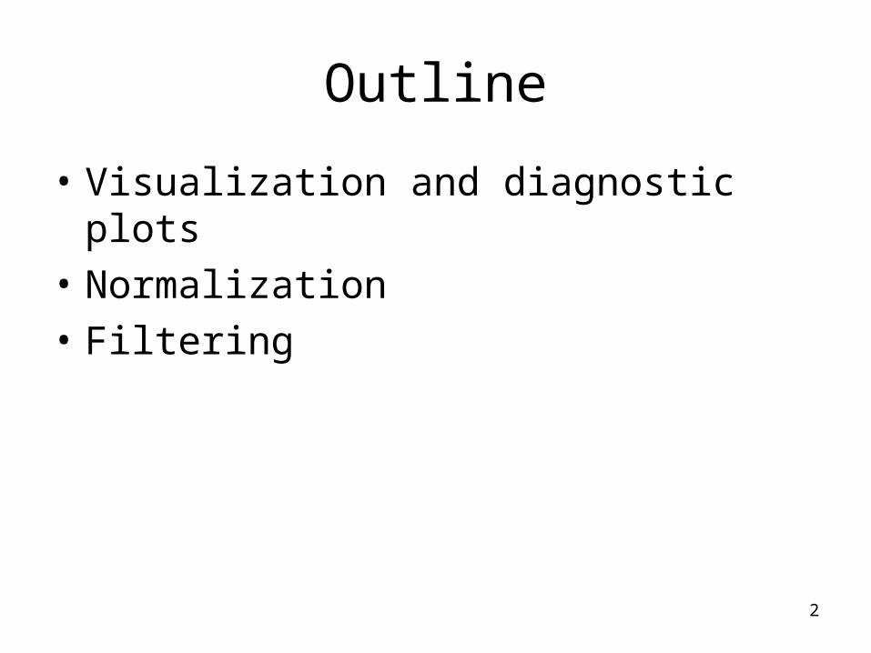
Outline

• Visualization and diagnostic plots• Normalization• Filtering

3

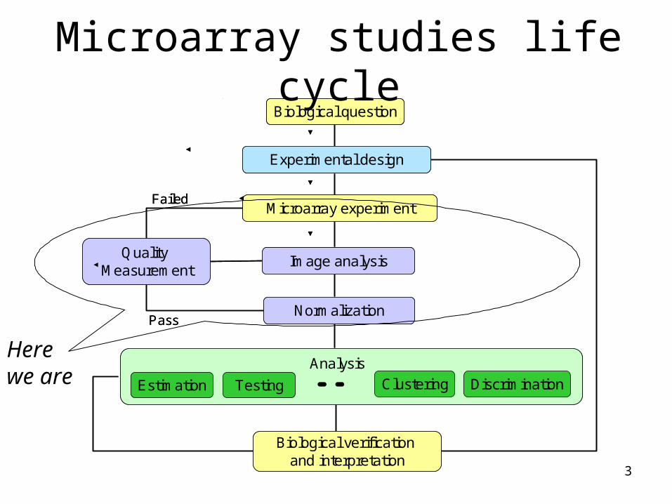
Quality Measurement

Biological verification and interpretation

Microarray experiment

Experimental design

Image analysis

Normalization

Biological question

TestingEstimation Discrimination

Analysis

Clustering

Failed

Pass

Quality Measurement

Biological verification and interpretation

Microarray experiment

Experimental design

Image analysis

Normalization

Biological question

TestingEstimation Discrimination

Analysis

Clustering

Failed

Pass

Microarray studies life cycle

Here we are

Looking at microarray dataDiagnostic Plots

Was the experiment a success?

5

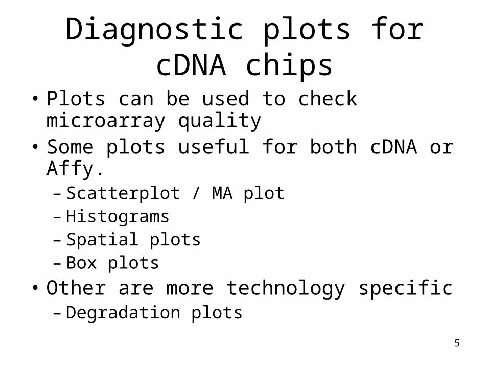
Diagnostic plots for cDNA chips

• Plots can be used to check microarray quality

• Some plots useful for both cDNA or Affy.– Scatterplot / MA plot– Histograms– Spatial plots– Box plots

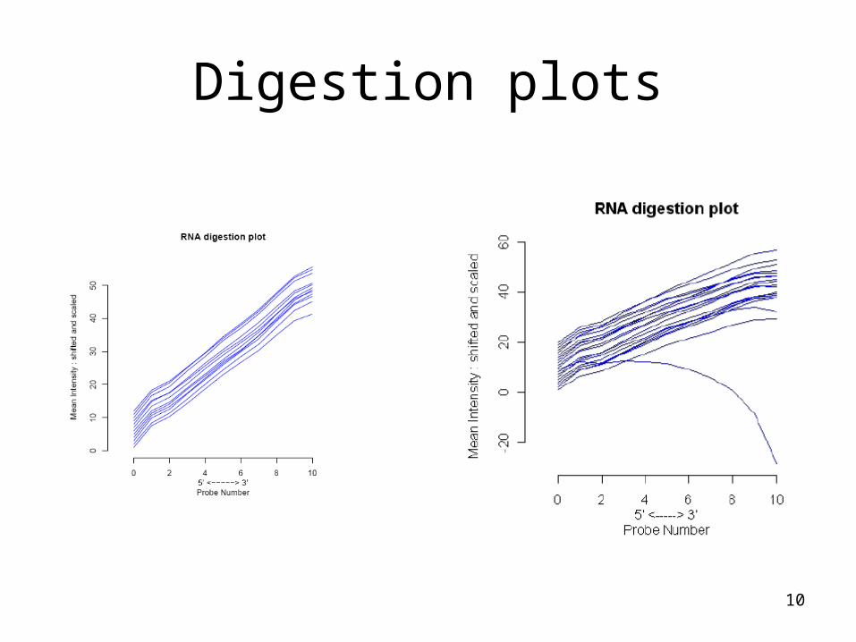
• Other are more technology specific– Degradation plots

6

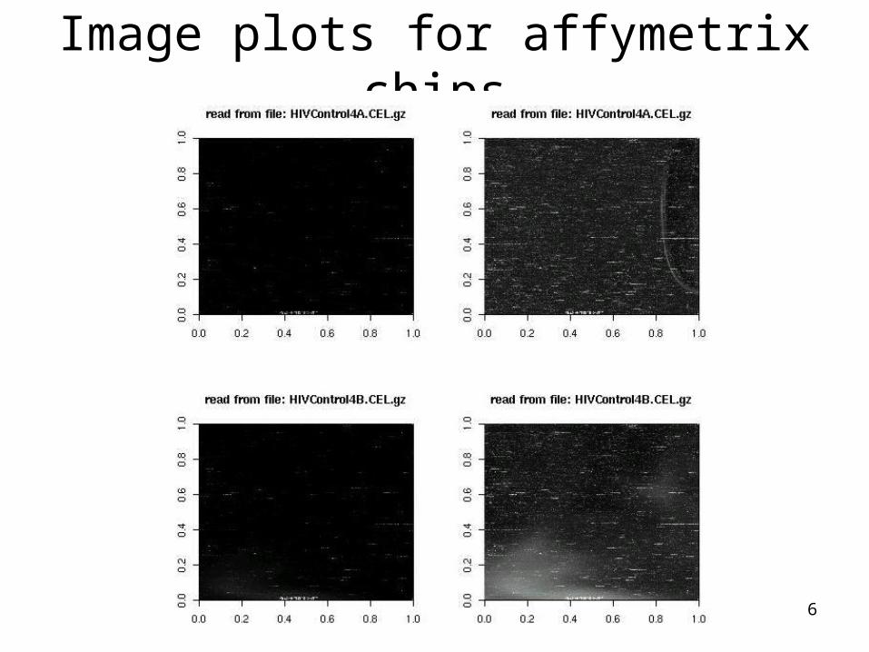
Image plots for affymetrix chips

7

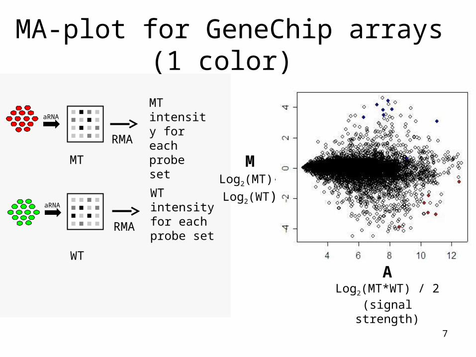
MA-plot for GeneChip arrays (1 color)

MT

WT

RMA

MTintensity for each probe set

RMA

WTintensity for each probe set

aRNA

aRNA

MLog2(MT)- Log2(WT)

ALog2(MT*WT) / 2(signal strength)

8

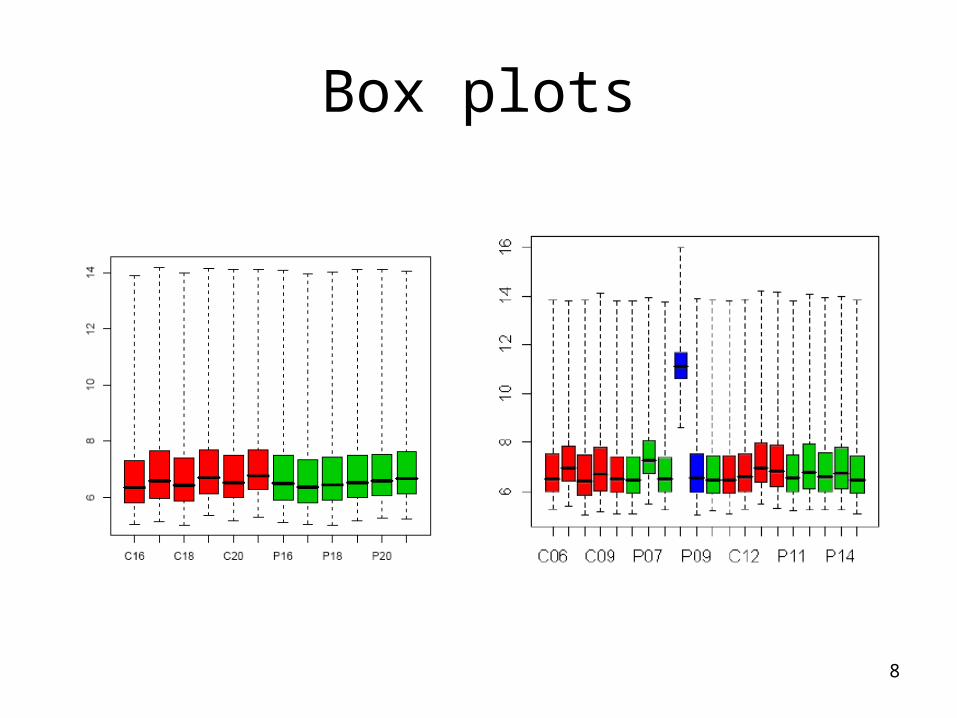
Box plots

9

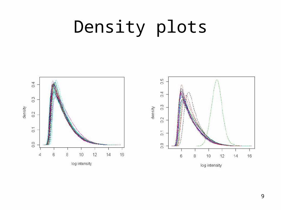
Density plots

10

Digestion plots

Preprocessing affy chips

12

Preprocessing steps

• Computing expression values for each probe set requires 3-steps– Background correction– Normalization– Probe set summaries

13

Most popular approaches

• Affymetrix’s own MAS 5 or GCOS 1.0 algorithms• RMA (Robust Multichip Analysis)

– Irizarry, Bolstad, Collin, Cope, Hobbs, Speed

(2003), Summaries of Affymetrix GeneChip probe level data. NAR 31(4):e15

• dChip http://www.dchip.org: Li and Wong (2001). Model-based analysis of oligonucleotide arrays: expression index computation and outlier detection. PNAS 98, 31-

14

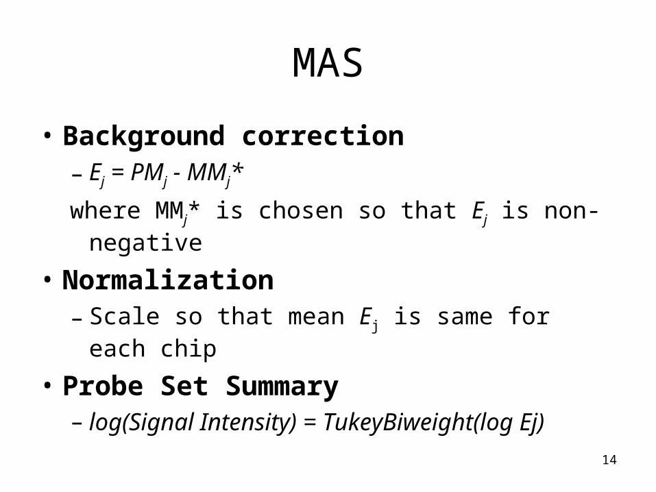
MAS

• Background correction– Ej = PMj - MMj*

where MMj* is chosen so that Ej is non-negative

• Normalization– Scale so that mean Ej is same for each chip

• Probe Set Summary– log(Signal Intensity) = TukeyBiweight(log Ej)

15

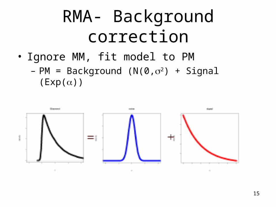
RMA- Background correction

• Ignore MM, fit model to PM– PM = Background (N(0,2) + Signal (Exp())

16

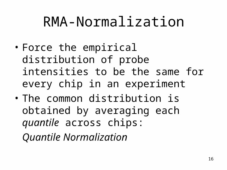
RMA-Normalization

• Force the empirical distribution of probe intensities to be the same for every chip in an experiment

• The common distribution is obtained by averaging each quantile across chips:

Quantile Normalization

17

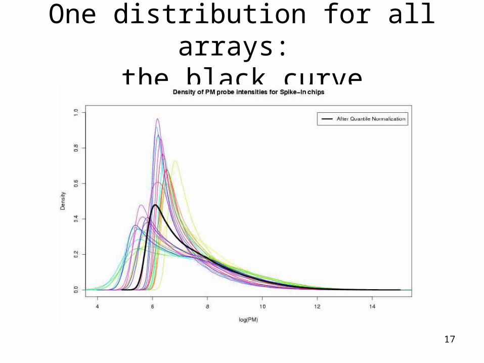
One distribution for all arrays: the black curve

18

RMA: Probe set summary

• Robustly fit a two-way model yielding an estimate of log2(signal) for each probe set

• Fit may be by – median polish (quick) or by – Mestimation (slower but yields standard errors

and good quality

• RMA reduces variability without loosing the ability to detect differential expression

19

MA plots before and after RMA

20

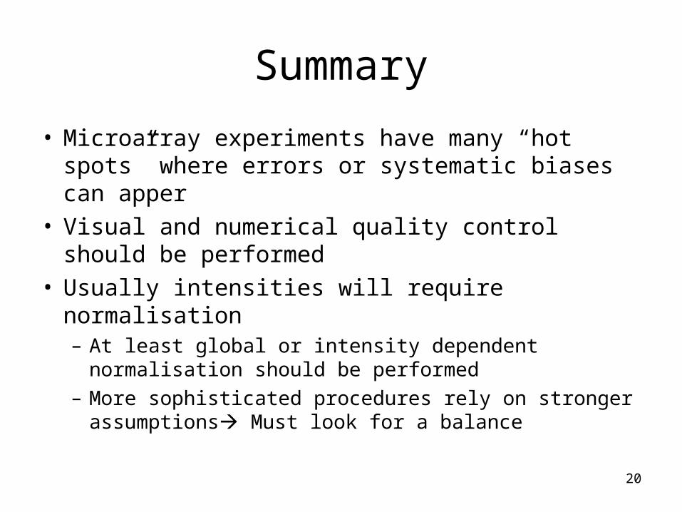
Summary

• Microarray experiments have many “hot spots” where errors or systematic biases can apper

• Visual and numerical quality control should be performed

• Usually intensities will require normalisation– At least global or intensity dependent normalisation

should be performed– More sophisticated procedures rely on stronger

assumptions Must look for a balance