mexico: fiscal sustainability
TRANSCRIPT

Report No. 20236-ME
Mexico:Fiscal Sustainability(In Two Volumes) Volume II: Background Papers
June 13, 2001
Mexico Country Management UnitPREM Sector Management UnitLatin America and the Caribbean Region
u
Document of the World Bank
Pub
lic D
iscl
osur
e A
utho
rized
Pub
lic D
iscl
osur
e A
utho
rized
Pub
lic D
iscl
osur
e A
utho
rized
Pub
lic D
iscl
osur
e A
utho
rized

CURRENCY EQUIVALENTSCurrency Unit - Mexican Peso (mxp$)
EXCHANGE RATE MARCH 17, 20009.35 MXP / 1 USD
WEIGHTS AND MEASURESMetric System
FISCAL YEARJuly I - June 30
ABBREVIATIONS AND ACRONYMSADE Acuerdo de Apoyo Inmediato a Deudores de la BancaADEFAS Adeudos de Ejercicios Fiscales AnterioresASA Aeropuertos y Servicios AuxiliaresBANCOMEXT Banco Nacional de Comercio Exterior, S.N.C.BANJERCITO Banco Nacional del Ejercito, Fuerza Aerea y Armada, S.N.C.BANOBRAS Banco Naciona] de Obras y Servicios Publicos, S.N.C.BANRURAL Banca Nacional de Credito Rural, S.N.C.BoM Banco de MexicoCAPUFE Caminos y Puentes Federales de Ingresos y Servicios ConexosCFE Comisi6n Federal de ElectricidadCNBV Comisi6n Nacional Bancaria y de ValoresCONASUPO Compafdia Nacional de Subsistencias PopularesEMBI Emerging Market Bond IndexFAMEVAL Fondo de Apoyo al Mercado de ValoresFARAC Fideicomiso de Apoyo a] Rescate de Autopistas
FIDEC Fondo para el Desarrollo ComercialFIDELIQ Fideicomiso Liquidario de Instituciones y Organizaciones Auxiliares del CreditoFINA Financiera Nacional AzucareraFINAPE Programa para el Financiamiento del sector Agropecuario y PesqueroFIRA Fideicomisos Instituidos en Relaci6n con la AgriculturaFNM Ferrocarriles Nacionales de MexicoFOBAPROA Fondo Bancario de Protecci6n al AhorroFOPYME Programa de Apoyo Financiero y Fomento a la Micro, Pequeina y Mediana EmpresaFOVI Fondo de Operaci6n y Financiamiento Bancario a la ViviendaGDP Gross Domestic ProductIMF International Monetary FundIMSS Instituo Mexicano del Seguro SocialINEGI Instituto Nacional de Estadistica, Geografia e InformaticaIPAB Instituto de Protecci6n al Ahorro BancarioISSSTE Instituto de Seguridad y Servicios Sociales de los Trabajadores del EstadoLFC Luz y Fuerza del CentroLOTENAL Loteria Nacional para la Asistencia PublicaMXP Mexican PesosNAFINSA Nacional Financiera, S.N.C.NIPA National Income Products AccountOECD Organization for Economic Co-operation and DevelopmentPEMEX Petr6leos MexicanosPIPSA Productora e Importadora de PapelSCNM Sistema de Cuentas Nacionales de MexicoSCT Secretaria de Comunicaciones y TransporteSHCP Secretaria de Hacienda y Credito PublicoVAT Value Added Tax
The Bank team that produced this report was headed by Stephen Everhart (LCSPE)-task manager, under the guidance ofMarcelo Giugale (LCCIC)-program team leader. Members of the Bank team include: Craig Bumside (DECRG), JoostDraaisma (LCCIC), Robert Duval (LCCIC), Andrew Feltenstein (IMF, Virginia Tech), Russ Murphy (Virginia Tech),Claudia Sepulveda (LCSPR), and Aaron Schwartzman (Emst & Young-Mexico). Production assistance was provided byMichael Geller and Elizabeth Toxtle (LCC IC).
The Bank appreciates the invaluable support and advice of Eliana Cardoso (LCSPE) and Vicente Fretes-Cibils(LCC4C). This study was undertaken under the general direction of Mr. Olivier Lafourcade (Director, LCCIC). Peerreviewers are: Messrs. Luis Serven (Lead Specialist - Regional Studies, LCSPR) and Anwar M. Shah (PrincipalEvaluation Officer, OEDCR).

VOLUME I: EXECUTIVE SUMMARYTABLE OF CONTENTS
Fiscal Sustainability-Mexico: A Synthesis
Rationale for the Study ..................................................... 1lIssues and Focus ...................................................... 2Fiscal Policy, Business Cycles, and Growth in Mexico ...................................................... 2Infrastructure, Extemal Shocks, and Mexico's Fiscal Accounts .......................... 3...........................3Infrastructure, Private Costs, and Payoffs from Additions to Infrastructure ................................................... 5Fiscal Impact of Contingent Liabilities ...................................................... 6Fiscal Deficit, Public Debt, and Fiscal Sustainability in Mexico ..................................................... 10An Extension: Balance Sheet Approach and Quality of Fiscal Adjustments ....................... I ........................ 16
The Mexican Case ..................................................... 19Implications of the Balance Sheet Approach ..................................................... 23
Conclusions: The Link Between Fiscal Sustainability and Fiscal Reform ................................................... 25References ..................................................... 27
List of Tables
Table E. 1 Estimate of the Overall Cost of the Financial Rescue, June 1999Table E.2 Contingent Liabilities Recognized by the Federal GovernmentTable E.3 Mexico Federal Debt as a Percentage of GDP
List of Figures
Figure E. 1 Concentration and Growth of Subnational Debt, 1994-1998: Selected StatesFigure E.2 Gross Federal Debt as Percent of GDP: Intemational BenchmnarksFigure E.3 Selected Latin American Eurobond SpreadsFigure E.4 Mexico Budget Indicators: 1980 - 1998Figure E.5 Tax Revenue as Percent of GDP, Selected Countries 1992 - 1998Figure E.6 Primary Deficit vs. Public Investment (percent of GDP)Figure E.7 Primary Deficit vs. Public Investment (percent of GDP) 5 UMI CountriesFigure E.8 Primary Deficit vs. Public Investment (percent of GDP) 6 LMI CountriesFigure E.9 Primary Deficit vs. Privatization Revenues (percent of GDP)Figure E. 10 Primary Deficit vs. Public Investment (percent of GDP) MexicoFigure E. 11 Primary Deficit vs. General Government Consumption (percent of GDP) MexicoFigure E. 12 Public Investment vs. Oil Prices MexicoFigure E. 13 Prograrnmable Expenditure Decomposition (percent of GDP) Mexico.Figure E. 14 Primary Deficit vs. Privatization Revenues (percent of GDP) MexicoFigure E. 15 Deficit Reduction and Oil DependenceFigure E.16 Components of Tax Revenues as a Percent of GDP, Mexico 1980-1998
iii

VOLUME II: BACKGROUND PAPERSTABLE OF CONTENTS
Chapter 1. Fiscal Policy, Business Cycles, and Growth in Mexico
Perspectives on Mexico's Fiscal Accounts from 1980-98 .............................................. 2The Business Cycle in Mexico ............................................. 3Trends and Cycles in Mexico's Fiscal Accounts ............................................. 6The Cyclically Adjusted Budget Surplus in Mexico ............................................. 16Methods for Computing the Cyclically Adjusted Budget Surplus ................. ............................. 17Budget Surplus Estimates for Mexico .............................................. 19How Fiscal Policy and Output Affect Each Other in Mexico .............................................. 23A Small VAR Model of the Mexican Economy ............................................. 24How Does the Fiscal Surplus Affect Output? ............................................. 25Dynamnic Behavior of the Fiscal Surplus ............................................. 27Policy Conclusions ............................................. 29References ............................................. 31Appendix ......................................... 33
Chapter 2. Infrastructure, External Shocks, and Mexico's Fiscal Accounts
Background ...................................... 43Model Structure ...................................... 45Production ...................................... 46Ba.ank.ing ...................................... 48Consumption ...................................... 48The Government ...................................... 49The Foreign Sector and Exchange Rate Determination ...................................... 49Money Supply ...................................... 50Data Sources, Calibration, and Simulation ...................................... 50Simulations ...................................... 55The Benchrnark Case ...................................... 55A Shock to Confidence in the Banking System ...................................... 55Trade Shock ...................................... 57Conclusion ...................................... 60References ...................................... 61Appendix ...................................... 62
Chapter 3. Infrastructure, Private Costs, and Payoffs from Additions to Infrastructure
Background ...................................... 68The Model ...................................... 72The Data ...................................... 74Sanple Horizon ...................................... 75Limitations ...................................... 75Estimation of the Model ...................................... 76Methods ....................................... 76Infreastructure ...................................... 76Estimation Limitations ...................................... 77Results .. . . . . . . . . . . . . . . . . . . . . . . . . . . . . . . . . . . . . . 78Overview ...................................... 79
iv

Payoffs from Additions to Infrastructure ........................................................................ 84Static Costs and Benefits of Increased Infrastructure ........................................................................ 85Optimal Infrastructure Stocks ........................................................................ 86Conclusions ....... ................................................................. 87References ....... ................................................................. 88Appendices ....... ................................................................. 90
Chapter 4. Fiscal Impact of Contingent Liabilities: The Case of Mexico
Coverage of the Study ........................................................................ 107Government Accounting Issues ........................................................................ 110Methodology ........................................................................ 111Deposit Insurance Scheme for Private Banks ......................... ............................................... 112The 1995 Banking Crisis ........................................................................ 113Expected Fiscal Costs of Resolution of the Crisis ........................................................................ 114Government Credit Assistance Programs ........................................................................ 120Characteristics of Direct Loans and Loan Guarantees ........................................................................ 121Expected Fiscal Cost of Government Credit Programs and the Budget ......................... ............................ 126Liabilities Related to Social Security Programs .............................. .......................................... 127The Financial Condition of IMSS ........................................................................ 127The Financial Condition of ISSSTE ........................................................................ 128Expected Fiscal Costs of Social Security Programs and the Budget ................................. ......................... 129Private Provision of Infrastructure and Government Guarantees ........................................... .................... 129Power Plants ....... ................................................................. 129Highways ........................................................................ 130The Fiscal Cost of Government Insurance Programs ................................................................. ....... 130Policy Implications ........................................................................ 132References ........................................................................ 134
Chapter 5. Fiscal Deficit, Public Debt and Fiscal Sustainability in Mexico
The Mexican Fiscal Accounts: Stylized Facts ........................... ............................................. 138Debt Management ........................................................................ 140Budget Indicators ........................................................................ 142Tax System ....... ................................................................. 143Government Expenditure Comnposition ........................................................................ 146Is Mexican Fiscal Policy Sustainable? ........................................................................ 148Accounting Approach to Fiscal Solvency ........................................................................ 148Pricing Approach to Fiscal Solvency ........................................................................ 149Intertemporal Approach to Fiscal Solvency: The Medium and Long Term ................. ............................. 151The Short and Medium Term ........................................................................ 152The Long Term: A Time Series Analysis 1980:01-1999:05 ....................................................................... 154Testing the Interternporal Budget Constraint: Unit Roots ........................................................................ 155The Case of a Stochastic Discount Rate ........................................................................ 156Testing for a Change in Regime ........................................................................ 157Testing the Intertemporal Budget Constraint: A Co-integration Approach .................. ............................. 160Testing Long-Run Relationship Between Government Spending Inclusive of Interest Payments andRevenue ....... ................................................................. 161Testing Long-Run Relationship Between Govermnent Spending Exclusive of Interest Payments,Interest Payments and Revenue ........................................................................ 163Policy Conclusions ........................................................................ 165References ........................................................................ 167Appendix ........................................................................ 169
v

List of Tables
Table 1.1 Sunmmary Budget Figures, 1980-81 1997-98Table 1.2 Cyclical Properties of Public sector Revenue and ExpenditureTable 1.3 Main Components of Public Sector Revenue and Expenditure, 1980-81 and 1997-98Table 1.4 Estimnates of Revenue and Expenditure ElasticitiesTable 1.5 Impulse Response Functions from the VARTable 1.6 Variance Decomposition of OutputTable 1.7 Variance Decomposition of the Unadjusted Primary Fiscal SurplusTable l.Al Estimates of a Piecewise Linear Trend in the Logarithm of Seasonally Adjusted Real GDPTable 2.1 Real GDP, 1980-97Table 2.2 Stocks of Infrastructure, 1970-90Table 2.3 Cost Elasticities by Sector and Infrastructure TypeTable 2.4 A Benchmark Simulation, 1995-2000Table 2.5 Reduction in the Interest Elasticity of Money Demand, 1995-2000Table 2.6 Interest Elasticity Decline Combined with an Infrastructure Increase 1995-200Table 2.7 Trade Shock: Real World Income Stagnates, 1995-2000Table 2.8 Trade Shock Combined with an Infrastructure Increase, 1995-2000Table 2.9 Infrastructure Elasticities = 0Table 3.1 Compound Annual Growth Rates 1960-93Table 3.2 Infrastructure Compound Annual Growth Rates, 1960-93 and 1983-93Table 3.3 Physical Infrastructure, Average Annual Growth RatesTable 3.4 Correlations: Physical and Financial Infrastructure MeasuresTable 3.5 Primary Data: Means and Standard DeviationsTable 3.6 Estimated Private Sector Cost Elasticities with Respect to Public Infrastructure StocksTable 3.7 Estimated Private Sector Cost Elasticities with Respect to Public Infrastructure StocksTable 3.8 Estimated Private Sector Cost Elasticities with Respect to Public Infrastructure StocksTable 3.9 Estimated Private Sector Cost Elasticities with Respect to Public Infrastructure StocksTable 3.10 Mean ElasticitiesTable 3.11 Static Cost and Benefits of Increased InfrastructureTable 3.12 Optimal Infrastructure StocksTable 3.13 OLS Panel ElasticitiesTable 3.14 OLS Random Effects ElasticitiesTable 3.15 FGLS Elasticities - Hetero, ARITable 3.16 Growth Rates Used for Nominal Electricity InfrastructureTable 3.17 Coefficient EstimatesTable 3.18 Coefficient Estimates (se's in (s), Dunmy Variables ExcludedTable 4.1 Fiscal Risk MatrixTable 4.2 Federal Insurance Programs with Major Fiscal RisksTable 4.3 State Government DebtTable 4.4 State Government Pension Liabilities: 1997Table 4.5 Pro Forma Balance Sheet of FOBAPROA, February 1998Table 4.6 Estimation of the Cost of the Financial Rescue, June 1999Table 4.7 Executed Fiscal Cost on Programs of Financial and Debtors RescueTable 4.8 Estimates of Total Losses of Resolving Major Bank InsolvensesTable 4.9 Government Loans by Major Program Area, Fiscal 1997Table 4.10 IMSS Retirement System Actuarial Deficit, December of 1994Table 4.11 Government Net Liability as a Result of the 1995 Pension ReformTable 4.12 Pro Forma Balance Sheet of FARAC as of November 1998Table 4.13 Contingent Liabilities and Fiscal Deficit AdjustmentsTable 4.14 Contingent Liabilities Recognized by the Federal GovernmentTable 5.1 Accounting Approach Mexico in 1998Table 5.2 Short and Medium-Term Indicators of Fiscal Sustainability as a percentage of GDPTable 5.3 Testing for Nonstationarity in Undiscounted and Discounted Net Public Debt, 1980:01-
1999:05
vi
Table 5.4 The Zivot Andrews Unit Root Test for Undiscounted and Discounted Public DebtTable 5.5 Testing for Nonstationarity in Real Interest Rates, 1980:1-1998:07Table 5.6 Testing for Nonstationarity in Real Government Spending Inclusive Interest Payments
and Government Revenues, 1980:1-1999:05Table 5.7 Results of Co-integration Government Spending Inclusive Interest Payments and
Government Revenue, 1980:01-1999:05Table 5.8 Testing for Nonstationarity in Real Government Spending, Interest Payments and Government
Revenues, 1980:1-1999:05Table 5.9 Results of Co-integration Noninterest Government Spending, Interest Payments and Government
Revenue, 1980:01-1999:05
List of Figures
Figure 1.1 Real GDP in Mexico, 1980-98Figure 1.2 Seasonally Adjusted Real GDP, 1980-98Figure 1.3 (a) Trends and Cycles in Real GDP: HP TrendFigure 1.3 (b) Trends and Cycles in Real GDP: Deviations from TrendFigure 1.4 Trends in Public Sector Revenues, 1980-98Figure 1.5 Cyclical Components of Revenue, 1980-98Figure 1.6 Trends in Public Sector Expenditure, 1980-98Figure 1.7 Cyclical Components of Expenditure, 1980-98Figure 1.8 The Budget Surplus and the Fiscal Imnpulse, 1980-98Figure 1.9 Cyclical Fluctuation in Output Caused by Fiscal ShocksFigure l.Al Trends in Real GDPFigure l .A2 Cyclical comnponents of Real GDPFigure 3.1 Changes in Electric, Transport, and Communications InfrastructureFigure 3.2 Education Infrastructure IndexFigure 4.1 Contingent Liabilities related to Potential Crisis of the Banking SectorFigure 5.1 Mexico Public Net Debt and Primary Deficit (+) as a percentage of GDP, 1980 - 1998Figure 5.2 Mexico Overall and Primary Deficit (+) as a percentage of GDP, 1980-1998Figure 5.3 Mexico Domestic and Foreign Public Net Debt as a percentage of GDP, 1980-1998Figure 5.4 Public Sector Domestic Debt as a percentage of GDP, 1982-1998Figure 5.5 Mexico Public Foreign Debt: Term Structure, 1982-1998Figure 5.6 Mexico Budget Indicators, 1980-1998Figure 5.7 Total Tax Revenues as a percentage of GDP-Selected CountriesFigure 5.8 Oil Revenues as a percentage of Total RevenuesFigure 5.9 Seignorage as a Source of Government RevenueFigure 5.10 Federal Government Revenue Tax MixFigure 5.11 Total Expenditure of the Central Government as a percentage of GDP-Selected CountriesFigure 5.12 Total Governnent Expenditure (million p$1994)Figure 5.13 Expenditure CompositionFigure 5.14 Real Annualized Interest Rate CETES 28 daysFigure 5.15 Brady Bonds DiscountsFigure 5.16 EMBI Spread RateFigure 5.17 Credit Rating for Mexico (100 lowest chance of default)Figure 5.18 Mexican Net Public Debt, 1980:1 - 1999:5. Undiscounted at Market Value (in Bill. P$ 1994)Figure 5.19 Sequential Zivot-Andrews Unit Root Test for the Mexican Undiscounted and Discounted Public
Net Debt, 1980:1-1999:5Figure 5.20 Government Spending Inclusive Interest and Govermment Revenues, 1980:1-1999:5Figure 5.21 Governrment Spending, Interest Payments and Government Revenues: 1980:01-1999:05
vii


1FISCAL POLICY, BUSINESS CYCLES, AND GROWTH IN MEXICO
1.1 This chapter investigates one aspect of the sustainability of fiscal policy in Mexico. Itfocuses on the role fiscal policy plays in detennining output in the short and medium term. Italso looks at how fiscal policy, in turn, responds to the business cycle. Finally, it investigates thepersistence of fiscal policy and how the authorities can use this persistence to forecast thegovernment's financing needs.
1.2 The chapter looks at these particular issues for a number of reasons. A traditional rolefiscal policy plays in industrial economies is that of a cyclical stabilizer. Fiscal policy istypically designed to "lean against the wind." That is, it is usually designed to stimulate outputwhen the economy moves into recession and to be contractionary when an expansion broadens.This is usually accomplished in two ways. The first way is by having components in the budgetthat respond automatically to the business cycle, such as tax revenues (which respond positively)or unemployment benefits (an expenditure item that responds negatively). The second way is byusing discretionary components in the budget to provide a stimulus during bad times. A fiscalpolicy designed in this way leads to a strongly procyclical budget surplus.
1.3 Mexico's fiscal policy does not lean against the wind. The analysis in this chapter willshow that the budget surplus is quite strongly countercyclical, so that fiscal policy leans with thewind. The automatic stabilizers in place are weak, and are further weakened by the tendency ofanother automatic component of the budget, oil-based revenue, which responds sensitively toexogenous world oil prices, to move countercyclically. Furthermore, the discretionarycomponent of the budget surplus also tends to move countercyclically.
1.4 If fiscal policy simply did not matter, then whether or not it leaned with or against thewind would be of little consequence. However, in Mexico, as in many other countries, fiscalpolicy does matter. The analysis suggests that an increase in the discretionary surplus of 1percent of gross domestic product (GDP) causes GDP to decline by 0.6 percent in less than ayear. Because in Mexico such increases typically occur during contractions, and thesecontractions are relatively short-lived (typically less than two years), this implies thatdiscretionary policy exacerbates the cycle.
1.5 The results imply that Mexico's fiscal policy lacks a design that makes it a stabilizingfeature of the economy. Furthermore, it has not been designed to render itself more sustainable.With procyclical fiscal policy (a countercyclical fiscal surplus), deficits cause debt to accumulateduring economic expansions, but when the economic expansion inevitably ends, this debtsuddenly becomes extremely costly. To finance it, the government must either take drasticdiscretionary fiscal measures, or it must finance the debt by borrowing at high real interest rates,

Chapter I
or by printing money and inducing rapid inflation. No matter which action the governmenttakes, the implications are similar: a worsening of the economic downturn. This chapter isintended to encourage policymakers to forrnulate fiscal policies that can smooth, rather thanexacerbate, real cycles, and that are therefore more readily sustained in the medium term.
1.6 The chapter begins by looking at the data. The sample period studied here-1980through mid-1998-spans several episodes in recent Mexican economic history. The choice ofperiod was largely driven by the availability of data. Quarterly national accounts data forMexico are available from 1980 onward, while monthly fiscal accounts are available from 1977onward. Trends and cycles in national accounts measures of real GDP are identified. Similarly,with GDP-based definitions of the business cycle in mind, this section describes the trends andcyclical fluctuations observed in various components of the public sector's fiscal accounts.
1.7 The second section of the chapter introduces the concept of the cyclically adjusted budgetsurplus. Historically, the main role of cyclically adjusted budget surplus measures has been astools in policy analysis in the knowledge that cyclical movements in output affect the publicsector's budget surplus. Cyclically adjusted budget surplus measures attempt to factor cyclicaleffects out of conventional measures. Once this is done, the adjusted measures are taken to beindicators of the stance of fiscal policy. This section examines a preferred definition of thecyclically adjusted budget surplus for Mexico. A question that naturally arises is whether this, orany other, adjusted budget measures are of particular use in policy analysis.
1.8 The third section of the chapter moves on to a more complex analysis of the data. Ratherthan working with simple indicators of the stance of fiscal policy, this section builds a simplestructural model of the Mexican economy that isolates several important features, namely:
* The nature of the feedback rule that implicitly determines fiscal policy, including theeffects of economic activity on the budget
- The exogenous shocks to the budget- The short- and medium-run effects of these shocks on economic activity* The extent to which forecasting the public sector's financing requirement is possible.
1.9 The main purpose of such a model is that the summary measures presented in the secondsection are typically useful in the context of a narrowly defined economic model. Furthermore,those summary measures are generally used to describe the effects of current policy on currentactivity. As such, given the lags with which fiscal policy is implemented and its effects are felt,the more forward-looking analysis of the third section should be of greater use to policymakers.
Perspectives on Mexico's Fiscal Accounts from 1980-98
1.10 This section examines quarterly data on Mexico's fiscal accounts from 1980 through mid-1998. While monthly budget data are available dating back to 1977, high-frequency data onGDP are only available from 1980 on. This section starts by defining the business cycle inMexico with reference to quarterly data on real GDP from the national accounts. It then dividesthe fiscal accounts into their revenue and expenditure components and looks at trends in revenueand expenditure.
2

Chapter I
The Business Cycle in Mexico
1.11 Figure 1.1 illustrates the behavior of real GDP in Mexico from 1980 through 1998. Theraw data show a clear pattern of seasonality. Overlying the general upward trend and cycles is apattern that indicates relatively low production in the first and third quarters and relatively highproduction in the second and fourth quarters. To identify these underlying features in the data, aseasonal adjustment filter was applied to the data.'
Figure 1.1 Real GDP in Mexico, 1980-98
1500 -
1400 -
1300-
1200-
1100
1000
900
800
80 81 82 83 84 85 86 87 88 89 90 91 92 93 94 95 96 97 98
Source: National accounts.
1.12 Figure 1.2 shows the seasonally adjusted figures. This figure also delineates recessionsusing shading.2 Several episodes are worth noting namely:
* The recession of 1982 through mid-1983 associated with the debt crisis* The period of slow growth thereafter, followed by the recession of late 1985 and 1986* The implementation of the stabilization program in 1988, with an initial, slightly
recessionary, year* The long expansion of 1989-94* The short and intense recession of 1995 associated with the peso crisis and the
subsequent recovery.
1. The adjustment procedure mimics the X - 11 seasonal adjustment procedure used by the U.S. Bureau of theCensus.
2. The following definitions of expansions and recessions were used to generate the shading in figure 1.2. If theeconomy was not already deemed to be in a recession and seasonally adjusted real GDP fell for two successivequarters, these quarters were marked as the beginning of a recession. Until seasonally adjusted real GDP rose fortwo successive quarters, all subsequent quarters were also deemed to be part of the same recession. A similar,but opposite, definition was used to define an expansion, with the further assumnption that at the beginning of thesample (first quarter of 1980), the economy was in an expansion.
3

Chapter 1
Figure 1.2 Seasonally Adjusted Real GDP, 1980-98
1600
1500
~1300
1200-
1100
1000
900
80080 81 82 83 84 85 86 87 88 89 90 91 92 93 94 95 96 97 98
Source: Author's calculations.
1.13 One way to describe the cyclical properties of fiscal policy would involve comparing thebehavior of revenue and expenditure during recessions to their behavior during expansions.However, with reference to figure 1.2, such an approach would clearly be unsatisfactory, becauseall expansions and all contractions are not alike. For example, the downturn after the peso crisisof December 1994 was much sharper and deeper than the ones experienced during the previousrecessions. It involved a cumulative decline in output of 9.7 percent, versus 6.8, 4.7, and 0.8percent in the previous recessions, and lasted two quarters, compared with six, five, and threequarters in the previous recessions. Similarly, the expansion since that recession has been morerapid than any of the previous expansions.
1.14 Furthermore, whether revenue and expenditure will differ according to whether output isrising or falling, rather than differing according to whether output is high or low is not obvious.The extent to which output, Y,, is high or low is typically measured with regard to some
benchmark, Y,<. That is, the business cycle is typically defined as Y,' = Y, / Y, . The literature
uses a number of benchmarks that can be the basis of a measure of the business cycle:
* The level of potential output* The trend in output as defined by a linear, possibly piecewise, trend in its logarithm* The trend in output as defined by the Hodrick and Prescott (HP) (1997) filter* The permanent component in output as defined by the Beveridge and Nelson (1981)
decomposition* The trend in output as defined by a peak-to-peak trend line.
4
Chapter 1
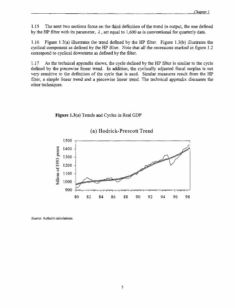
1.15 The next two sections focus on the third definition of the trend in output, the one definedby the HP filter with its parameter, A, set equal to 1,600 as is conventional for quarterly data.
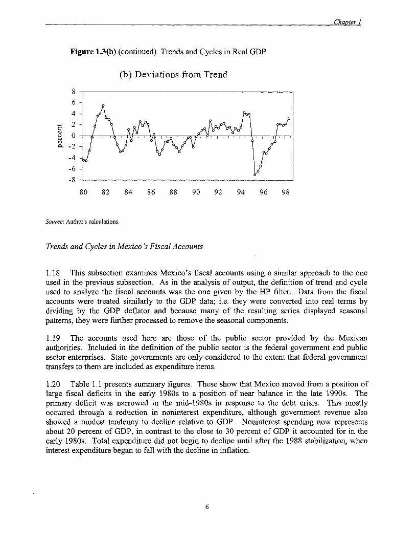
1.16 Figure 1.3(a) illustrates the trend defined by the HP filter. Figure 1.3(b) illustrates thecyclical component as defined by the HP filter. Note that all the recessions marked in figure 1.2correspond to cyclical downturns as defined by the filter.
1.17 As the technical appendix shows, the cycle defined by the HP filter is similar to the cycledefined by the piecewise linear trend. In addition, the cyclically adjusted fiscal surplus is notvery sensitive to the definition of the cycle that is used. Similar measures result from the HPfilter, a simple linear trend and a piecewise linear trend. The technical appendix discusses theother techniques.
Figure 1.3(a) Trends and Cycles in Real GDP
(a) Hodrick-Prescott Trend
1500 -
X 1400-
1300-
1200-
1100-
1000 I
900 -
80 82 84 86 88 90 92 94 96 98
Source: Author's calculations.
5
Chapter 1
Figure 1.3(b) (continued) Trends and Cycles in Real GDP
(b) Deviations from Trend
8- 6 -
0 -
-4-
-6-
80 82 84 86 88 90 92 94 96 98
Source: Author's calculations.
Trends and Cycles in Mexico 's Fiscal Accounts
1.18 This subsection examines Mexico's fiscal accounts using a similar approach to the oneused in the previous subsection. As in the analysis of output, the definition of trend and cycleused to analyze the fiscal accounts was the one given by the HP filter. Data from the fiscalaccounts were treated similarly to the GDP data; i.e. they were converted into real terms bydividing by the GDP deflator and because many of the resulting series displayed seasonalpatterns, they were further processed to remove the seasonal components.
1.19 The accounts used here are those of the public sector provided by the Mexicanauthorities. Included in the definition of the public sector is the federal government and publicsector enterprises. State governments are only considered to the extent that federal governmenttransfers to them are included as expenditure items.
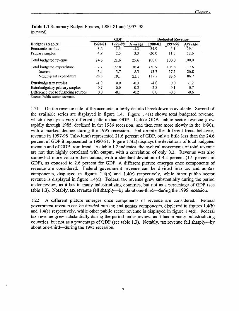
1.20 Table 1.1 presents summary figures. These show that Mexico moved from a position oflarge fiscal deficits in the early 1980s to a position of near balance in the late 1990s. Theprimary deficit was narrowed in the mid-1980s in response to the debt crisis. This mostlyoccurred through a reduction in noninterest expenditure, although government revenue alsoshowed a modest tendency to decline relative to GDP. Noninterest spending now representsabout 20 percent of GDP, in contrast to the close to 30 percent of GDP it accounted for in theearly 1980s. Total expenditure did not begin to decline until after the 1988 stabilization, wheninterest expenditure began to fall with the decline in inflation.
6
Chapter I
Table 1.1 Summary Budget Figures, 1980-81 and 1997-98(percent)
GDP Budgeted RevenueBudget category: 1980-81 1997-98 Average 1980-81 1997-98 AverageEconomic surplus -8.6 -1.3 -5.3 -34.9 -6.1 -19.4Primary surplus -4.9 2.5 3.3 -20.0 11.5 12.6
Totalbudgetedrevenue 24.6 21.6 25.6 100.0 100.0 100.0
Total budgeted expenditure 32.2 22.8 30.4 130.9 105.8 117.6Interest 3.4 3.7 8.3 13.7 17.1 30.8Noninterestexpenditure 28.8 19.1 22.1 117.2 88.6 86.7
Extrabudgetary surplus -1.0 0.0 -0.3 -4.0 0.0 -1.2Extrabudgetary primary surplus -0.7 0.0 -0.2 -2.8 0.1 -0.7Difference due to financing sources 0.0 -0.1 -0.2 0.0 -0.3 -0.6Source: Public sector accounts.
1.21 On the revenue side of the accounts, a fairly detailed breakdown is available. Several ofthe available series are displayed in figure 1.4. Figure 1.4(a) shows total budgeted revenue,which displays a very different pattern than GDP. Unlike GDP, public sector revenue grewrapidly through 1985, declined in the 1986 recession, and then rose more slowly in the 1990s,with a marked decline during the 1995 recession. Yet despite the different trend behavior,revenue in 1997-98 (July-June) represented 21.6 percent of GDP, only a little less than the 24.6percent of GDP it represented in 1980-81. Figure 1.5(a) displays the deviations of total budgetedrevenue and of GDP from trend. As table 1.2 indicates, the cyclical movements of total revenueare not that highly correlated with output, with a correlation of only 0.2. Revenue was alsosomewhat more volatile than output, with a standard deviation of 4.4 percent (1.1 percent ofGDP), as opposed to 2.6 percent for GDP. A different picture emerges once components ofrevenue are considered. Federal government revenue can be divided into tax and nontaxcomponents, displayed in figures 1.4(b) and 1.4(c) respectively, while other public sectorrevenue is displayed in figure 1.4(d). Federal tax revenue grew substantially during the periodunder review, as it has in many industrializing countries, but not as a percentage of GDP (seetable 1.3). Notably, tax revenue fell sharply-by about one-third--during the 1995 recession.
1.22 A different picture emerges once components of revenue are considered. Federalgovernment revenue can be divided into tax and nontax components, displayed in figures 1.4(b)and 1.4(c) respectively, while other public sector revenue is displayed in figure 1.4(d). Federaltax revenue grew substantially during the period under review, as it has in many industrializingcountries, but not as a percentage of GDP (see table 1.3). Notably, tax revenue fell sharply-byabout one-third---during the 1995 recession.
7

Chapter I
Figure 1.4. Trends in Public Sector Revenue, 1980-98
(a) Total Budgeted Revenue (b) Tax Revenue
ss________________ . __________ 40
75 355
65 3
45 20
90 8Z 84 86 S8 90 92 94 96 98 80 82 84 86 98 90 92 94 96 98
(c) Non-Tax Federal Revenue (d) Other Public Sector Revenue
25 145220
235
so 30
~~~~~~~~t5~~~~~~~~~~~~220
80 92 94 86 98 90 92 94 96 98 S0 S2 S4 96 SS 90 92 94 96 98
(e) Income Tax Revenue (h Revenue from Goods & Services Taxes
2 0 - _2___.5
is to0
o t
oo
90 92 84 96 99 90 92 94 96 9S go 92 94 36 99 90 92 94 96 99
(g) Revenue from Trade Taxes (h) Revenue from Hydrocarbon Fees
22 ~ ~ ~ ~ ~ ~ ~~~~~~~~~~~2
.14
90 9 2 94 86 99 90 92 94 96 99 to 92 84 36 99 90 92 94 96 98
(i) Revenue ofPEMEX (j) OtherNon-GovtPublic Sector Ravcoue
24- 24 -
20
2 96~~~~~~~~~~~~~~~~~2
012 16-
12
4
90 92 94 86 99 90 92 94 96 9n so 92 94 96 98 90 92 94 96 98
Source: Public sector- accounts.
8
Chapter I
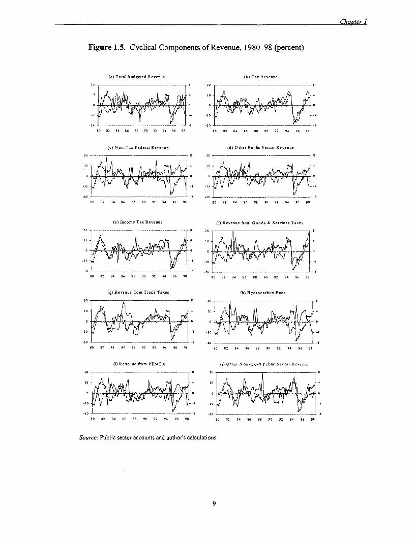
Figure 1.5. Cyclical Components of Revenue, 1980-98 (percent)
(a) Total Budgeted Revenue (b) Tax Revenue
14 - . .................... . 8 20
;. Y fd -4 0 -4
S0 82 84 86 88 90 92 94 96 98 S0 82 84 86 B8 90 92 94 96 98
(c) N on-Tax Federal Revenue (d) Other Public Sector Revenue
60 S8 0 8
(e) Inom Tax 4eeu ceu rmGos&Srie ae
-30 is
60 1 - 8 230 __ -.80 82 84 86 88 90 92 94 96 98 80 82 84 86 88 90 92 94 96 98
(e) Income Tax Revenue (t Revenue from Goods & Services Taxes
-60 -8 20 -8
80 82 84 86 88 90 92 94 96 98 80 82 94 86 88 90 92 94 96 98
(i) Revenue from Trade Taxe Othe ) Hydo carbon'Pbi FecoRes eu
60 5° 1 4
30 4~~~~~~~~~~~~~~~~~~-
-30 -8 -30
80 82 84 86 85 90 92 94 96 98 90 82 84 86 88 90 92 94 96 98
(i) Revenue from Trad X Tax O he Nutonoo Pbl SctorReven
60 9 20- 9
30 4 30 [ -
0 . 0 0 -
-30- -4 tO0 -4
60.3 -60------.- _________________________ -8
S0 82 84 86 88 90 92 94 96 98 80 82 84 86 88 90 92 94 96 98
Source: Reeucfo PM X(j thTN n-o' Public Sector acontendathrnuacuaios
60 20- 9~~~~~~~~
Chapter I
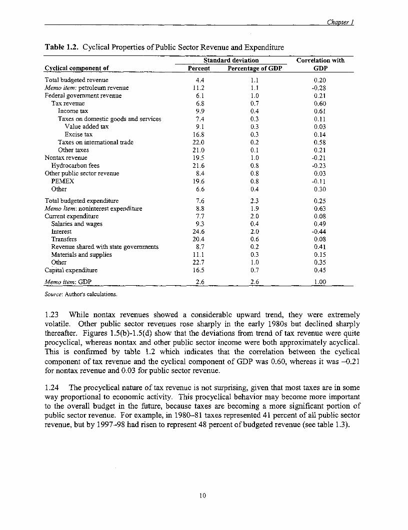
Table 1.2. Cyclical Properties of Public Sector Revenue and Expenditure
Standard deviation Correlation withCyclical component of Percent Percentage of GDP GDP
Total budgeted revenue 4.4 1.1 0.20Memo item: petroleum revenue 11.2 1.1 -0.28Federal government revenue 6.1 1.0 0.21
Tax Tevenue 6.8 0.7 0.60Income tax 9.9 0.4 0.61Taxes on domestic goods and services 7.4 0.3 0.11
Value added tax 9.1 0.3 0.03Excise tax 16.8 0.3 0.14
Taxes on international trade 22.0 0.2 0.58Other taxes 21.0 0.1 0.21
Nontax revenue 19.5 1.0 -0.21Hydrocarbon fees 21.6 0.8 -0.23
Other public sector revenue 8.4 0.8 0.03PEMEX 19.6 0.8 -0.11Other 6.6 0.4 0.30
Total budgeted expenditure 7.6 2.3 0.25Memo Item: noninterest expenditure 8.8 1.9 0.63Current expenditure 7.7 2.0 0.08
Salaries and wages 9.3 0.4 0.49Interest 24.6 2.0 -0.44Transfers 20.4 0.6 0.08Revenue shared with state governments 8.7 0.2 0.41Materials and supplies 11.1 0.3 0.15Other 22.7 1.0 0.35
Capital expenditure 16.5 0.7 0.45
Memo item: GDP 2.6 2.6 1.00
Source: Author's calculations.
1.23 While nontax revenues showed a considerable upward trend, they were extremelyvolatile. Other public sector revenues rose sharply in the early 1980s but declined sharplythereafter. Figures 1.5(b)-l.5(d) show that the deviations from trend of tax revenue were quiteprocyclical, whereas nontax and other public sector income were both approximately acyclical.This is confirmed by table 1.2 which indicates that the correlation between the cyclicalcomponent of tax revenue and the cyclical component of GDP was 0.60, whereas it was -0.21for nontax revenue and 0.03 for public sector revenue.
1.24 The procyclical nature of tax revenue is not surprising, given that most taxes are in someway proportional to economic activity. This procyclical behavior may become more importantto the overall budget in the future, because taxes are becoming a more significant portion ofpublic sector revenue. For example, in 1980-81 taxes represented 41 percent of all public sectorrevenue, but by 1997-98 had risen to represent 48 percent of budgeted revenue (see table 1.3).
10

Chapter I
Table 1.3. Main Components of Public Sector Revenue and Expenditure, 1980-81 and 1997-98(percent)
GDP Budgeted revenueBudget category: 1980-81 1997-98 Average 1980-81 1997-98 Average
Total budgeted revenue 24.6 21.6 25.6 100.0 100.0 100.0Memo item: petroleum revenue 8.2 7.4 9.5 33.3 34.1 36.3Federalgovernmentrevenue 14.6 15.1 15.6 59.3 69.8 61.5
Taxrevenue 10.1 10.3 10.4 41.2 47.7 41.0Income tax 5.1 4.3 4.5 20.8 20.0 17.9Taxes on domestic goods and services 3.5 4.9 4.7 14.4 22.7 18.4
Value added tax 2.6 3.1 2.9 10.4 14.5 11.5Excise tax 1.0 1.8 1.8 4.1 8.2 6.9
Taxes on intemational trade 1.0 0.6 0.8 4.3 2.6 3.0Other taxes 0.4 0.5 0.4 1.7 2.4 1.6
Nontax revenue 4.5 4.7 5.2 18.2 21.9 20.4Hydrocarbon fees 3.7 3.1 3.8 15.0 14.2 14.8
Other public sector revenue 10.0 6.5 10.0 40.7 30.1 38.5PEMEX 4.1 2.3 4.1 16.8 10.8 15.3Other 5.9 4.2 5.9 23.9 19.4 23.1
Totalbudgeted expenditure 32.2 22.8 30.4 130.9 105.8 117.6Memo item: noninterest expenditure 28.8 19.1 22.1 117.2 88.6 86.7Current expenditure 23.5 20.0 26.0 95.8 92.6 100.2
Salaries and wages 5.8 3.4 4.7 23.5 15.8 18.4Interest 3.4 3.7 8.3 13.7 17.1 30.8Transfers 2.9 5.0 2.8 11.7 23.2 11.5Revenue shared with state governments 2.2 3.0 2.7 9.1 14.0 10.6Materials and supplies 3.5 1.6 3.0 14.2 7.2 11.5Other 5.9 3.3 4.4 23.9 15.1 17.2
Capital expenditure *8.8 2.9 4.4 35.9 13.3 17.5
Source: Public Sector accounts.
1.25 Despite their overall procyclical nature, the trends and cycles across various taxcategories exhibit some interesting differences. Figures 1.4(e)-1.4(g) show the most importantcomponents of tax revenue: income tax; taxes on domestic goods and services, namely, valueadded tax (VAT) and excise tax; and taxes on international trade, which are dominated by importtaxes.
1.26 Table 1.3 shows that domestic goods and services taxes have been an increasinglyimportant part of revenue. In 1997-98 these taxes represented 48 percent of all tax revenues,versus 35 percent in 1980-81. Most of this increase has come from taxes of petroleum products:more than half of the increase in VAT receipts has come from PEMEX. Excise taxes on gasolinehave risen sharply, while other excise taxes have fallen. Taxes on domestic goods and servicesare the only tax component that appears to have been rising significantly during the study period.Income taxes have risen somewhat, while taxes from international trade are roughly at the samelevels now as they were in 1980, thus both have fallen as a share of revenue and GDP. Thedeclining reliance on import duties, the slow expansion of income taxation, and the expansion ofVAT are typical of countries at Mexico's stage of development. However, scope exists for thefurther expansion of VAT on commodities other than petroleum.
11

Chapter l
1.27 As concerns cyclical properties, figures 1.5(e)-1.5(g) show the cyclical components ofthe three types of taxes. Income taxes are clearly highly procyclical (table 1.2 indicates that thecorrelation with the cyclical component of GDP is 0.61), though clearly more volatile than thebusiness cycle itself. Taxes on domestic goods and services are not particularly procyclical (thecorrelation with GDP is just 0.11), but this pattern appears to have been changing since 1994.Revenue from trade taxes is highly procyclical (the correlation with GDP is 0.58), reflecting thehighly procyclical nature of imports.
1.28 The sole large component of nontax revenue is hydrocarbon fees, which are included infederal government revenue under one classification scheme, although they are sometimesclassified as PEMEX revenue.3 They are plotted in figure 1.4(h). They display little overalltrend, currently represent about 14 percent of all budgeted revenue, and have been somewhatcountercyclical (the correlation with GDP is -0.23), as indicated by Figure 1.5(h).
1.29 The single largest component of rest of public sector revenue is the revenue of PEMEX,which is displayed in figure 1.4(i). Even when hydrocarbon fees are classified as governmentrevenue PEMEX still represents 11 percent of all budgeted revenue and more than a third of therevenue generated by the nongovemrnment public sector. Although PEMEX's contribution hasdeclined in significance from about 17 percent of revenue in 1980-81, this figure is misleading.If all petroleum-based revenue is aggregated across the public sector, it currently represents 34percent of revenue as opposed to 33 percent of revenue in 1980-81 (see table 1.3). As figure1.5(i) indicates, and table 1.2 confirms, PEMEX's contribution to revenue is somewhatcountercyclical: the correlation with GDP is _0.11 .4
1.30 The rest of the public sector has declined slightly as a source of revenue (see table 1.3)and has somewhat procyclical income as indicated by figure 1.5(j) and table 1.2. Among theimportant contributors are the electrical utilities and railways.
1.31 On the expenditure side of the public sector flow of funds, a distinction will be madebetween interest on public debt and other forms of spending. Noninterest expenditure fell in theearly 1980s, as indicated in figure 1.6(a). This occurred just as interest expenditure (figure 1.6h)accelerated with the inflation rate. As table 1.3 indicates, noninterest expenditure has fallensharply as a fraction of GDP, from 29 percent in 1980-81 to just 19 percent in 1997-98. At thesame time, the public sector has moved to a substantial primary surplus position on budget, withbudgeted noninterest expenditure now representing 89 percent of budgeted revenue, as opposedto 117 percent in 1980-81. Interestingly, noninterest expenditure is highly procyclical, asindicated by figure 1.7(a) and table 1.2. The correlation of its cyclical component with thecyclical component of GDP is 0.63, and it is substantially more volatile than GDP with astandard deviation of 8.8 percent (1.9 percent of GDP), compared with 2.6 percent for GDP(table 1.2). This procyclical behavior of expenditure offsets the procyclical behavior of revenueand tends to make the primary budget close to neutral with respect to the cycle. As a recentstudy by the Inter-American Development Bank indicated (Gavin and others 1996), the public
3. In the "B" accounts of the Secretaria de Hacienda y Credito Puiblico the revenues from hydrocarbons areclassified as government revenue, but in the "G" accounts they are classified as revenues of PEMEX.Consolidation across the entire public sector makes this accounting difference irrelevant.
4. Looking more narrowly, the export revenues of PEMEX, which are more closely tied to the world oil price, aremore strongly countercyclical: the correlation with GDP is -0.29.
12
Chapter I
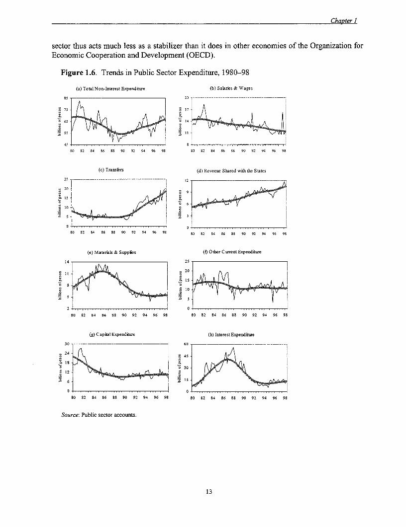
sector thus acts much less as a stabilizer than it does in other economies of the Organization forEconomic Cooperation and Development (OECD).
Figure 1.6. Trends in Public Sector Expenditure, 1980-98
(a) Total Non-Interest Expenditure (b) Salaries & Wages
85 20 -
o75- 1 -1
O65-~ 14-
55 1
45i 8S0 82 84 j6 88 90 92 94 96 98 S0 82 84 86 88 90 92 94 96 98
(c) Transfers (d) Revenue Shared with the States
25- 12
20-
10 O
.05
80 82 84 86 88 90 92 94 96 9S S0 82 84 86 8 90 92 94 96 98
(e) Materials & SuppEes (f) Other Current Expenditure
14- 25-
09 ~ ~ ~ ~ ~ ~ ~ ~ ~~~~~0
5-
(g) C apital Expenditure (h) Interest Expenditure
30 ~ ~ ~ ~ ~ ~ ~ ~~~~~~324
0. 19~ ~~~~~~~~~~~~~~1
80 82 84 86 88 90 92 94 96 98 80 82 84 86 88 90 92 94 96 98
Source: Public sector accounts.
13

Chapter I
Figure 1.7. Cyclical Components of Expenditure, 1980-98(percent)
(a) TotalNon-Interest Expenditure (b) Salaries & Wages
24- _ 8 40-
12- 4 20~ 4
0 k0 0 ~
-12- -4 -20-
-24 -8 -40 -8
80 82 84 86 88 90 92 94 96 98 80 82 84 86 88 90 92 94 96 98
(c) Transfers (d) Revenue Shared with the States
30- 4 15- 4
0 0 0 0
-30 ~ 4 1 -4
-60 - -- -30 -S
80 82 84 86 88 90 92 94 96 98 80 82 84 86 88 90 92 94 96 98
(e) Materials & Supplies () Other Current Expenditure
30-- 8 7018
is V 4 35- 4
0 - m A 0 0 - A ~~~~ 19.0A
-45 -8 7 0
80 82 84 86 88 90 92 94 96 98 80 82 84 86 88 90 92 94 96 98
(g) Capital Expendiure (h) Interest Expenditure
50 -- 8 80 ------- - ----------------- ---- 8
25- 4 40
0- 0W A N 0
-25 -4 -40 -
-5 ----5__._-- _ 8-0 ---- _............................................ _ ___ ..
80 82 84 86 88 90 92 94 96 98 80 82 84 86 88 90 92 94 96 98
Source: Public sector accounts and author's calculations.
1.32 Once expenditure is divided into its components, an even clearer picture emerges.Salaries and wages in the public sector, depicted in figure 1.6(b), have been declining in realterms almost steadily since 1980. Table 1.3 indicates that they now represent just 16 percent ofbudgeted revenue, compared with 24 percent in 1980-81. Most of the decline in the publicsector wage bill has been within the federal government, which is perhaps surprising given the
14

Chapter I
declining importance of the nongovernment component of the public sector. While the wage billhas fallen as the economy has expanded (figure 1.6b), figure 1.7(b) and table 1.2 indicate that themovements around this trend have been quite procyclical. Most of this procyclical behavior isnot due to the federal government wage bill, but is largely determined by the behavior of wageswithin the corporate public sector.5
1.33 Transfers have become an increasingly significant component of the overall public sectorbudget, as indicated by figure 1.6(c). By 1997-98 they represented 23 percent of budgetedrevenue as opposed to just 12 percent in 1980-81 (table 1.3). Because government transfers topublic sector corporations are netted out of this figure, this represents a substantial increase in theimportance of social programs within the economy. However, these transfers have not beencountercyclical as one might have expected. If anything, transfer payments appear to beprocyclical: figure 1.7(c) shows that spending on transfers rose rapidly during the early l990sand then declined sharply during the 1995 recession. On the other hand, table 1.2 indicates that,overall, transfers have been approximately acyclical.
1.34 The lack of cyclical variation in transfer payments deserves some further explanation.The figures used in this chapter for "transfer payments" correspond to that portion of thegovernment's spending category "Aid programs, subsidies and transfers" that is classified ascurrent expenditure. In 1997 this amounted to about 200 billion pesos. Economic classificationof expenditure is available for the entire "Aid programs, subsidies and transfers" category withcapital expenditures included. In 1997 this amounted to about 230 billion pesos. So currentexpenditures make up the bulk of this category. The portion of this overall budget dedicated toaid programs or social assistance spending was only about 32 billion pesos or about 15 percent ofcurrent transfers. Most of the rest of the transfer budget represents revenue sharing, subsidies orfinancing to public sector entities. Given these facts, it is not surprising that transfer spending isapproximately acyclical.
1.35 The federal government shares a substantial portion of its revenue with states, and thisrevenue sharing has increased in importance, as indicated by figure 1.6(d). Revenue distributedto the states rose from 9 percent of budgeted revenue in 1980-81 to 14 percent in 1997-98 (table1.3). It has also been procyclical, its cyclical component having a correlation of 0.41 with thecyclical component of GDP (table 1.2). This is similar in magnitude to the correlation of overalltax revenue with GDP.
1.36 Because the nongovernment public sector is responsible for most of the expenditure onmaterials and supplies, the decline of this component of the public sector is responsible for thedecline in this expenditure relative to public sector revenue from 14 percent in 1980-81 to 7percent in 1997-98.6 This pattern is confirmed by figure 1.6(e). Materials and suppliesexpenditures are only slightly procyclical, as indicated by figure 1.7(e). The correlation of theircyclical component with GDP is just 0.15 (table 1.2).
5. Disaggregated figures not presented in Table 1.2 indicate that the federal governnent's wage bill has a cyclicalcorrelation with GDP of just 0. 18, while the figure for the rest of the public sector is 0.58.
6. Figures not presented in table 1.3 indicate that, on average, more than 90 percent of materials and suppliesexpenditure is accounted for in the nongovernment sector.
15

Chapter 1
1.37 Other current expenditure, illustrated in figure 1.6(f), consists of several items includingpayments for services rendered by the private sector. It has declined significantly as a share ofrevenue from 24 percent in 1980-81 to just 15 percent in 1997-98 (table 1.3). This is largelydue to a decline in this type of spending by the federal government. It is somewhat procyclicalas indicated by Figure 1.7(f), and has a correlation with GDP of 0.35 (table 1.2).
1.38 Capital expenditure is the last category of noninterest expenditure. This has declinedsignificantly since its peak in 1982. Capital expenditure has declined from 36 percent ofbudgeted revenue in 1980-81 to just 13 percent in 1997-98 (table 1.3). The federal governmenthas halved its capital spending from 1 4 to less than 7 percent of budgeted revenue, while the restof the public sector has seen an enormous decline in capital spending from 22 percent of revenueto less than 7 percent. Capital spending has been quite procyclical, as indicated by figure 1.7(g).Its correlation with GDP was 0.45 (table 1.2) during the entire study period. Indeed, duringsevere recessions such as those in 1982 and 1995, capital spending was cut sharply.
1.39 The final item is interest expenditure, illustrated in figure 1.6(h). Inflation effects are thedriving force behind changes in the size of interest flows. Interest expenditure shot up in 1982and 1986, not only because public sector debt increased, but mainly because inflation accelerateddramatically. High real interest rates in the stabilization period after 1988 kept interestexpenditure at high lev-els, but declining debt eventually brought interest spending down. Itagain rose in significance in 1995 as inflation accelerated during the peso crisis, but by the timethe public sector's overall level of indebtedness was by then much lower than in the early 1980s.Interest expenditure is strongly countercyclical, its correlation with GDP being -0.45 (table 1.2),largely because in Mexico inflation has tended to be highest during periods of recession.
1.40 One way to deal with the inflation effects that dominate interest flows would be tocompute real rather than nominal interest flows. Even though the interest flows pictured infigure 1.6(h) are expressed in real terms (that is, they are expressed in constant peso termns), theyare nominal interest flows in the sense that they represent some average nominal interest ratetimes the nominal level of debt divided by the price level. Real interest flows, instead, would becomputed by calculating some average real interest rate times the nominal level of debt, dividedby the price level. Making accurate adjustments of this sort is quite difficult when a significantfraction of the debt is held outside Mexico and is denominated in many different foreigncurrencies. Furthermore, at times, significant portions of domestic debt have been indexed orissued in foreign currency. Hence no attempt at making inflation adjustments is made here. Thisis of little significance, because later sections argue that the focus should be on the primarybudget surplus, which excludes all interest expenditure.
The Cyclically Adjusted Budget Surplus in Mexico
1.41 This section outlines a methodological approach for computing cyclically adjusted budgetsurplus measures for Mexico. It examines several approaches that a variety of intemationalorganizations use and computes historical surplus figures using a preferred method. It then askswhether the adjusted surplus is a useful concept, that is, can it help policymakers make policydecisions?
16

Chapter I
Methods for Computing the Cyclically Adjusted Budget Surplus
1.42 Economists have long recognized that budget surplus figures tend to be procyclical. Inparticular, budget surpluses are procyclical in most OECD countries for a number of reasons thatwill be elaborated upon later. In the context of Keynesian macroeconomic theory, when thepublic sector runs a larger budget surplus than previously, the government is said to have acontractionary fiscal policy stance. However, if the budget surplus is larger simply because theeconomy is going through an expansionary phase of the business cycle, thinking of fiscal policyas contractionary may be inappropriate. Thus, many economists have proposed that budgetsurplus figures should somehow be adjusted to allow for the effects of the business cycle.
1.43 The literature on adjusted budget surplus measures can be traced back to the paper byBrown (1956), where he argued that to measure the stance of fiscal policy correctly one had todistinguish between "automatic" and "discretionary" policies. Brown's paper did not propose anadjusted measure of the budget surplus, because he explicitly argued in favor of the differentialtreatment of the various components of revenue and expenditure with reference to an explicitKeynesian model of the economy.
1.44 Since Brown's paper economists have sought a single indicator of the stance of fiscalpolicy, similar to the budget surplus as a percentage of GDP, but adjusted for the business cycle.A number of government and international agencies produce these sorts of measures includingthe OECD, the World Bank, the International Monetary Fund (IMF), the European Community(EC), and their various member goverunents. A number of indicators have been suggested.Chouraqui, Hagemann, and Sartor (1990) and Price and Muller (1994) present good discussionsof the various indicators. Blanchard (1990) and Buiter (1993) provide arguments against usingsingle indicators.
1.45 Cyclical adjustment of the budget usually begins with the decomposition of output intosome trend, or potential, component and its cyclical component. The technical appendixdescribes several methods including the one used here: the same method that the EC uses (seeEC 1995 for even greater detail regarding its method of estimating structural budget deficits),which adopts the HP filter-based trend in GDP as the measure of potential output.
1.46 To compute cyclically adjusted surplus measures the EC, IMF, and OECD estimate theelasticities of various components of revenue and expenditure with respect to output. They usethe estimated elasticities to make cyclical adjustments to these components of the budget.7 Atthis stage an important set of assumptions must be made: one must decide which revenue andexpenditure components fall into the automatic category and which fall into the discretionarycategory. Because the assumption is that the business cycle causes those that fall into theautomatic category, while those in the discretionary category potentially cause the cycle, onlythose components that fall into the automatic category should be adjusted.
7. Details of how the elasticities are estimated and used to make cyclical adjustments are provided in the technicalappendix.
17

Chapter I
1.47 For the purposes of this chapter, the following revenue and expenditure categories inMexican data were considered for adjustment:
* Income tax revenue, Rlt
* Taxes on domestic goods and services, excluding gasoline, R2 t
* Taxes on intemational trade, excluding taxes on PEMEX imports, R3t
* Other tax revenue, R4t
* Governnent transfers net of transfers to the public sector, X, .
Estimates of the elasticities of these revenue and expenditure categories with respect to thecyclical component of output are found in table 1.4. As the elasticity for transfer payments wasnot statistically significant, no adjustments to this item were made. Adjustments to the fourrevenue categories were made.
1.48 It should be reemphasized that the decision to adjust some revenue/expenditurecategories and not others is based on strong a priori assumptions about causality rather than on astatistical test. The notion is that tax revenues behave cyclically largely because most taxsystems rely on statutory tax rates on various types of economic activity-this naturally leads tocyclical movements in tax revenue. Similarly, in many countries transfer programs arestructured to respond automatically to business cycle movements. As a result, it seemsreasonable, from a theoretical perspective, to treat the cyclical movements of tax revenues andtransfers as being driven by the various factors that drive the business cycle, rather than being thecauses, themselves, of the business cycle. Expenditure categories such as wages and salaries andcapital expenditure are highly procyclical, but they are typically not adjusted for the cycle-theimplicit argument against adjustment is that these categories of expenditure are fundamentallymore discretionary. Of course, if all revenue and expenditure categories were adjusted theadjusted surplus would be uncorrelated, by construction, with the business cycle.
1.49 As described in more detail in the technical appendix, the adjusted surplus measure isgiven by
(1) At = At - Rj, [exp (eR>y )-1
i=,
where A, is the standard budget surplus measure, ej1 is the elasticity of Rj, with respect to
output and y, is the cyclical component of output, as measured using the HP filter.
1.50 As table 1.3 indicates, oil revenue represents about a third of the Mexican public sector'sbudgeted revenue. There is some question as to whether the cyclically adjusted budget measuresshould also reflect this fact. On the one hand, if one wants to make adjustments that purelyreflect the business cycle's effect on the budget, one would make no adjustments to oil revenue.On the other hand, if the purpose of estimating a cyclically adjusted fiscal surplus is to isolatethose components of the budget that are not driven by exogenous forces, correcting for oil prices
18
Chapter I
is important. Two alternative measures of the cyclically adjusted budget surplus are presentedbelow: one that makes no adjustment for oil prices, !A, and one that does, namely:
(2) A, = A - RO[exp(eROpt )-1].
Here Rot represents petroleum revenue, eRG is the elasticity of the cyclical component of
petroleum revenue with respect to the cyclical component of the world oil price, and po is the
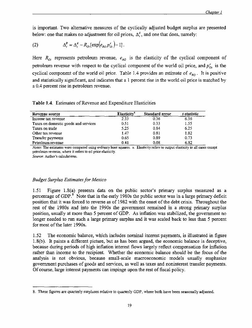
cyclical component of the world oil price. Table 1.4 provides an estimate of eRO. It is positive
and statistically significant, and indicates that a 1 percent rise in the world oil price is matched bya 0.4 percent rise in petroleum revenue.
Table 1.4. Estimates of Revenue and Expenditure Elasticities
Revenue source Elasticitya Standard error t-statisticIncome tax revenue 2.33 0.36 6.56Taxes on domestic goods and services 0.51 0.33 1.55Taxes on trade 5.25 0.84 6.25Other tax revenue 1.47 0.81 1.82Transfer paymnents 0.65 0.89 0.73Petroleum revenue 0.41 0.08 6.82Notes: The estimates were computed using ordinary least squares. a. Elasticity refers to output elasticity in all cases exceptpetroleum revenue, where it refers to oil price elasticity.Source: Author's calculations.
Budget Surplus Estimates for Mexico
1.51 Figure 1.8(a) presents data on the public sector's primary surplus measured as apercentage of GDP.8 Note that in the early 1980s the public sector was in a large primary deficitposition that it was forced to reverse as of 1982 with the onset of the debt crisis. Throughout therest of the 1980s and into the 1990s the government remained in a strong primary surplusposition, usually at more than 5 percent of GDP. As inflation was stabilized, the government nolonger needed to run such a large primary surplus and it was scaled back to less than 5 percentfor most of the later 1990s.
1.52 The economic balance, which includes nominal interest payments, is illustrated in figure1.8(b). It paints a different picture, but as has been argued, the economic balance is deceptive,because during periods of high inflation interest flows largely reflect compensation for inflationrather than income to the recipient. Whether the economic balance should be the focus of theanalysis is not obvious, because small-scale macroeconomic models usually emphasizegovernment purchases of goods and services, as well as taxes and noninterest transfer payments.Of course, large interest payments can impinge upon the rest of fiscal policy.
8. These figures are quarterly surpluses relative to quarterly GDP, where both have been seasonally adjusted.
19
Chapter 1
1.53 The cyclically adjusted primary balance is illustrated in figure 1.8(c). At first glance, thecyclically adjusted balance and the standard measure of the primary balance appear to be quitesimilar. The difference between the two measures is plotted in figure 1.8(e), and at times it issubstantial. Whenever it is negative, it indicates that fiscal policy was more contractionary thanindicated by the standard primary surplus. Whenever it is positive, fiscal policy was moreexpansionary than indicated by the standard primary surplus. Note, for example, that fiscalpolicy looks more expansionary during the 1990-94 with the adjusted budget figures.
1.54 The adjustments for petroleum revenue can also be substantial. Petroleum revenuemoves closely with the world oil price, which is highly volatile. Figure 1.8(f) shows thatadjustments of revenue for exogenous movements in oil prices have amounted to as much as 2percent of GDP. For example, oil revenue shot up in 1991 because of the Gulf War. Removingthis effect from the data requires an adjustment in the amount of 2 percent of GDP; however,figure 1.8(d) shows that the overall picture is little changed by taking movements in oil revenuedue to oil prices into account. Other factors dominate movement in the budget surplus.
1.55 Using the primary balance as a summary measure, Mexico's fiscal policy is procyclical inthe following sense. Countercyclical policy, or leaning against the wind, is usually described asrunning deficits during recessions and surpluses during expansions. In other words, policy iscountercyclical when the budget surplus is procyclical. However, the correlation betweenMexico's primary surplus as a percentage of GDP and the GDP's cyclical component, measuredin percent, is -0.35. This indicates that Mexico has tended to run higher surpluses during hardtimes and smaller surpluses or deficits during good times.
1.56 The cyclical adjustment of the primary surplus only makes this fact starker. Thecorrelation between the cyclically adjusted primary surplus and GDP is -0.44.9 This suggeststhat discretionary policy, rather than leaning against the wind, seems to lean quite strongly withthe wind.
1.57 The finding here is consistent with the discussion in Gavin and others (1996). They studya number of Latin American countries and find that in the typical country, fiscal policy is muchmore procyclical than in the OECD. Both revenue and expenditure are typically much moresensitive to the business cycle than in the OECD, but the expenditure effect is stronger.
1.58 This finding may reflect the fact that during recessions, Mexico's public sector, like thatin many Latin American countries, faces a hard budget constraint. Perhaps discretionary policycannot be expansionary in the traditional sense because the government is liquidity constrained.But this begs the question: how did the government become liquidity constrained in the firstplace? Was procyclical fiscal policy itself the culprit? Whatever the reason, policymakersshould note that policy moves with the business cycle rather than against it.
9. This is to be expected, because the cyclical component of the budget surplus is highly correlated with the cyclicalcomponent of GDP. The cycle- and oil-adjusted budget surplus has a correlation with GDP of -0.40.
20
Chapter I
Figure 1.8. The Budget Surplus and the Fiscal Impulse, 1980-98
(a) Primary Balance (b) Economic Balance
15 5-
-15 ^20 s !
80 82 84 86 88 90 92 94 96 98 80 82 84 86 88 90 92 94 96 98
(c) Cyclically-Adjusted Primary Balance (d) Cycle- and Oil-Adjusted Primnary Balance
15 - . ..............15!
10- C 101S........ 1.5 2.0
80 82 84 86 88 90 92 94 96 98 80 82 84 86 88 90 92 94 96 98
(c) Cy(ca) Cyciedbased PriAdjustm ent (BaOilh) Cycal OR-Adjust me nt s
1.5- 2.0
10- ~~~~~~~~~~~10-
o E
05
_ 0 \ .3 \ F 94\t ~~~~ 0.
--0.5-
10- ~~~~~~~~~~~~~~-10.-1.0 -1.0
80 82 84 86 88 90 92 94 96 98 80 82 84 86 88 90 92 94 96 98
(g)o Fiscale: se b Cyc lAdjustment (h m ls Adjustment s
2.5- 21
o ~~~~~~~~~~~~~~~~~10-0.5-
5-1 ~ ~ ~ ~ ~ ~ ~ ~ ~ ~ ~~~~~05 -
-2 1. -2
80 8 2 84 86 9 2 94 9 88 84 86 88 90 92 94 96 98 jS gour ical Ipublcseco bacdounts.eAjsmnt(Fsa mplebsdo Bt dutet
1~~~~~~~~~~~~2

Chapter 1
1.59 How are the cyclically adjusted budget figures useful to policymakers? Presumably theyare useful because they isolate the component of fiscal policy that is assumed to be exogenouswith respect to the business cycle from the part that is determined by the business cycle. Onecould argue that it is this component of policy that is discretionary, and policymakers should begiven some sense of the effects of these discretionary policies on economic activity.Underpinning the various approaches discussed is the assumption that a simple Keynesian modelcan be used to think about the economy. It is this model that allows the effects on output to beidentified. To summarize fiscal policy with one budget number one must assume that the sameKeynesian multiplier applies to government purchases of goods and services, taxes, and transferpayments. Because even the simplest Keynesian models are inconsistent with such anassumption, the possible limitations of the cyclically adjusted budget balance as an indicator offiscal policy are immediately obvious.
1.60 An altemative fiscal indicator that the IMF uses is the fiscal impulse (the discussion hereis loosely based on Chand 1993). This indicator compares the stance of fiscal policy in twosuccessive budget years, but it continues to treat governmnent purchases, taxes, and transfersvirtually symmetrically. The fiscal impulse measure is based on the so-called cyclical effect ofthe budget, which is defined as the difference between the actual budget surplus and the budgetsurplus that would have been achieved in the absence of discretionary policy. In its simplestform, this method treats all movements in government expenditure that are not proportional totrend output as discretionary. It further treats all changes in revenue because of changes in theaverage rate at which revenue is raised as discretionary. Thus the discretionary component of thebudget surplus is
AD = R, - rY, - (X, - xY,*)
=/, r-t )
where F is the ratio of revenue to output in a typical year, x is the ratio of expenditure to outputin a typical year, and the other variables are defined as before. The fiscal impulse is simplydefined as the negative of the change in the discretionary budget surplus, expressed as a fractionof GDP."'
1.61 The discretionary primary budget surplus for Mexico was calculated, along these lines,by setting r and x equal to their sample averages for 1980-98. The difference between theprimary budget balance and the discretionary primary budget balance is its nondiscretionarycomponent. While the IMF method makes bigger adjustments to the budget surplus fornondiscretionary fiscal policy than the methods described earlier, the overall picture remainsunchanged. The discretionary budget surplus remains countercyclical, and its correlation withthe cyclical component of GDP is -0.46. It is also highly correlated with the cyclically adjustedbudget surplus calculated previously. The correlation coefficient between the two series is0.998. Hence this section continues to use l .
10. The fiscal impulse is the negative of the change in the discretionary budget surplus, because budget deficits areassumed to provide a positive imnpulse to economic activity.
22

Chapter 1
1.62 The fiscal impulse, FI/A = _(YA _), in some sense measures the change in policy
stance. Whenever it is positive, policy is moving toward a more expansionary position. Figure1.8(g) shows the fiscal impulse calculated using the cyclically adjusted budget surplus, whilefigure 1.8(h) shows the fiscal impulse calculated using the cycle- and oil-adjusted budgetsurplus: FIB = -( _J - AB1). Both series are expressed as backward-looking, four-quarter,moving averages, because the quarterly observations are extremely volatile. The two measuresare almost perfectly correlated. They both indicate that in every case where Mexico has goneinto recession, fiscal policy has moved toward a more contractionary stance.
1.63 As Chand (1993) acknowledges, the IMF measure of discretionary fiscal policy, like thecyclically adjusted budget surplus measures, is somewhat flawed in that it treats governmentpurchases, transfers, and taxes symmetrically, at least with regard to the effects of theirdiscretionary components on output. Furthermore, the cyclically adjusted budget surplus andthe discretionary budget surplus are useful tools of policy analysis only to the extent that they areimportant factors in the determination of output. This is usually taken on faith, but whetherdiscretionary policy matters for economic activity, even if it is identified correctly, is notobvious. It will matter only if the economy behaves as if it were a simple Keynesian model. Thenext section addresses this issue for Mexico.
How Fiscal Policy and Output Affect Each Other in Mexico
1.64 Does discretionary fiscal policy actually affect output? Does it affect output in ways thatKeynesian macroeconomic models would predict? That is, is so-called expansionary fiscalpolicy actually expansionary? This section explores these questions in a more complexframework than the previous section by explicitly modeling the feedback between fiscal policyand output. Using a vector autoregressive (VAR) approach, the model is enhanced by explicitconsideration of oil prices (the main determinant of Mexico's terms of trade), the real exchangerate (a possible indicator of monetary policy, wealth effects, or public confidence), the U.S.Federal Funds rate (an indicator of U.S. monetary policy) and GDP in the United States (anindicator of the demand for Mexican exports).
1.65 The approach in the previous section is clearly somewhat limiting. Under the identifyingassumption that some revenue and expenditure components are endogenous to the business cyclewhile others are not, it allows the calculation of cyclically adjusted budget figures, but it does notpermit hypotheses about the dynamic effects of the cyclically adjusted budget to be tested.Furthermore, it does not take into account the full effects of such factors as the terms of trade,external demand, and world interest rates.
1.66 This section addresses the following questions using the VAR approach:
* How does discretionary policy affect economic activity?* What were the fiscal impulses to output in historical episodes?* Is there significant reverse causality from output to the budget not captured with the
methodology used in the previous section?
23

Chapter I
* Is there enough persistence in the budget to allow for short- or medium-term forecastingof financing?
The next subsection describes the time series included in the VAR. The second subsectionanswers the first two questions about effects on output. The third subsection deals with the lasttwo questions concerning feedback effects on the budget and the potential for forecasting.
A Small VAR Model of the Mexican Economy
1.67 A modified VAR is specified for a 6 x 1 vector of time series, zt, where z, consists of
* The logarithm of the world price of oil (expressed in constant 1993 pesos per barrel)* The logarithm of real GDP in the United States (measured in constant 1992 chained
dollars)* The U.S. federal funds rate (measured in percent per year)* The Mexican fiscal surplus (measured in percentage of GDP),* The logarithm of real GDP in Mexico (measured in constant 1993 pesos)* The logarithm of the real Mexico-U.S. exchange rate.
1.68 The logarithm of the oil price, pot, is included not only because oil prices affect thepublic sector budget balance, but also because they largely determine Mexico's terms of trade.They may therefore have an effect on economic activity as well as the real exchange rate. Thelogarithm of real GDP in the United States, Yut, is included because it can be used as an
exogenous indicator of the demand for Mexican exports. The U.S. Federal Funds rate, rut, isused as an indicator of monetary policy in the United States. Because Mexico's ability to borrowfunds might well depend on conditions in the world financial market, American monetary policyis likely to play some role in business cycle fluctuations in Mexico.
1.69 For the Mexican fiscal surplus the cycle- and oil-adjusted primary budget surplus as afraction of GDP, Xt = A, / Y,t, is used in the benchmark VAR. The unadjusted primary surplus
is also used to verify the robustness of the findings. The logarithm of Mexican real GDP, YMt, isincluded to examine the feedback between the fiscal surplus and output. Finally, the logarithmof the real exchange rate, s,, is included, because it is a useful variable that may reflect othershocks to wealth in Mexico, as well as short- and medium-term changes in Mexican monetarypolicy. The logarithm of the real exchange rate is measured as s* = ln(StP, / PF), where St is the
nominal exchange rate in pesos per dollar, P, is the U.S. GDP deflator, and P, is the MexicanGDP deflator.
1.70 So z, = (pot yut rut X YMt s7)t. The technical appendix describes how a
structural VAR model for zt can be identified, estimated, and used to answer the questionsposed.
24
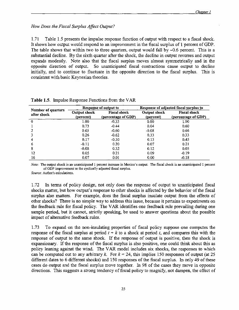
Chapter I
How Does the Fiscal Surplus Affect Output?
1.71 Table 1.5 presents the impulse response function of output with respect to a fiscal shock.It shows how output would respond to an improvement in the fiscal surplus of 1 percent of GDP.The table shows that within two to three quarters, output would fall by -0.6 percent. This is asubstantial decline. By the sixth quarter after the shock, the decline in output reverses and outputexpands modestly. Note also that the fiscal surplus moves almost symmetrically and in theopposite direction of output. So unanticipated fiscal contractions cause output to declineinitially, and to continue to fluctuate in the opposite direction to the fiscal surplus. This isconsistent with basic Keynesian theories.
Table 1.5. Impulse Response Functions from the VAR
Response of output to Response of adjusted fiscal surplus toNumber shofk quarte Output shock Fiscal shock Output shock Fiscal shock
(percent) (percentage of GDP) (percent) (percentage of GDP)a i.oo -0.33 0.00 1.001 0.73 -0.44 0.04 0.602 0.65 -0.60 -0.08 0.663 0.26 -0.62 0.33 0.334 0.17 -0.30 0.13 0.456 -0.11 0.20 0.07 0.218 -0.08 0.32 0.12 0.0512 0.05 0.21 0.09 -0.1916 0.07 0.01 0.00 -0.18
Note: The output shock is an unanticipated I percent increase in Mexico's output. The fiscal shock is an unanticipated I percentof GDP improvement in the cyclically adjusted fiscal surplus.
Source: Author's calculations.
1.72 In tenrs of policy design, not only does the response of output to unanticipated fiscalshocks matter, but how output's response to other shocks is affected by the behavior of the fiscalsurplus also matters. For example, does the fiscal surplus insulate output from the effects ofother shocks? There is no simple way to address this issue, because it pertains to experiments onthe feedback rule for fiscal policy. The VAR identifies one feedback rule prevailing during onesample period, but it cannot, strictly speaking, be used to answer questions about the possibleimpact of alternative feedback rules.
1.73 To expand on the non-insulating properties of fiscal policy suppose one computes theresponse of the fiscal surplus at period t + k to a shock at period t, and compares this with theresponse of output to the same shock. If the response of output is positive, then the shock isexpansionary. If the response of the fiscal surplus is also positive, one could think about this aspolicy leaning against the wind. The VAR model includes six shocks, the responses to whichcan be computed out to any arbitrary k. For k = 24, this implies 150 responses of output (at 25different dates to 6 different shocks) and 150 responses of the fiscal surplus. In only 49 of thesecases do output and the fiscal surplus move together. In 98 of the cases they move in oppositedirections. This suggests a strong tendency of fiscal policy to magnify, not dampen, the effect of
25
Chapter I
shocks on output, given the presumption that improvements in the fiscal surplus arecontractionary.
1.74 Another way to judge the importance of different shocks is the variance decomposition.The variance decomposition breaks forecast errors for each time series into their various sources.For examnple, if one were forecasting output four periods ahead, the forecast error would dependon unanticipated shocks to each of the variables in z,. The relative importance of the six shocks
will vary depending on the forecast horizon. If a shock is relatively important at short horizons,then it is a shock that has relatively short-lived, but important, effects on output; however, if ashock is relatively important at long horizons, then it has more of a long-run impact. Table 1.6illustrates the variance decomposition for Mexican GDP at different forecasting horizons.
Table 1.6 Variance Decomposition of Output(percentage of the variance of the forecast error)
Forecast Fraction of variance due to shocks to
horizon
(quarters) Oil prices U.S. GDP Federal funds Fiscal surplus GDP Real exchange rate
0 0.0 2.6 4.9 15.1 77.4 0.0
1 19.4 1.2 2.6 18.4 52.2 6.3
2 20.9 0.8 1.9 25.2 41.4 9.8
3 24.4 0.9 1.8 29.1 31.5 12.4
4 27.2 1.4 4.8 26.6 26.9 13.1
6 24.4 3.1 15.7 22.2 21.8 12.9
8 20.2 4.0 26.1 20.9 18.2 10.8
12 18.5 3.6 36.4 19.1 13.5 9.0
16 22.9 3.3 37.9 16.1 11.2 8.6
Source: Author's calculations.
1.75 The table indicates that fiscal shocks are in important source of fluctuations in GDP,especially at horizons of about two to six quarters, where they account for almost 25 percent ofthe variance in GDP. At the one-year horizon, fiscal shocks are as important as any other sourceof business cycle fluctuations. II
1.76 Another way to examine the importance of the budget for output is to compute ahistorical decomposition of fluctuations in GDP into their sources. This can be done quite easilyas a by-product of the VAR estimation. The decomposition divides all deviations of GDP fromtrend into seven components: a part due to conditions at the beginning of the sample period, andsix parts each due to the six different shocks in the VAR. Figure 1.9 plots the portion of GDPcaused by fiscal shocks. Note that the fiscal shocks have typically contributed a substantial
11. Notice that shocks to the real exchange rate have no effect on output at the 0 horizon because the real exchange
rate is placed last in the VAR ordering. This placement is based on the notion that all shocks to the economy,
both real and nominal, are likely to be quickly reflected in both prices and the nominal exchange rate. It is also
arguable, however, that one source of shocks to the fiscal surplus is the real exchange rate. If the real exchange
rate is placed before the fiscal surplus in the ordering then the impulse response of output with respect to a fiscalshock is in the same direction as indicated in Table 1.5, though a little less strong. On the other hand, the
variance decomposition does change significantly: for example at a horizon of 8 quarters real exchange rate
shocks and fiscal shocks account for 23 and 13 percent of the variation in output, respectively.
26

Chapter 1
portion of the variation in output, with the possible exception of the expansion of the early 1990swhich appears to have had little to do with fiscal expansion. The recession of 1995, also appearsnot to have been caused by contemporaneous or lagged fiscal shocks to any significant degree.
1.77 From this analysis it seems fair to conclude that the reforms of the late 1980s broughtwith them an improvement in budgetary institutions-fiscal policy has played a less directlydestabilizing role. This does not mean that the feedback rule for fiscal policy cannot play animportant stabilizing role in the future, through further institutional changes.
Figure 1.9. Cyclical Fluctuation in Output Caused by Fiscal Shocks
4-
-4-
-8
80 82 84 86 88 90 92 94 96 98
- Fiscal Shock Component + Cyclical Component of GDP
Source: Author's calculations.
Dynamic Behavior of the Fiscal Surplus
1.78 Table 1.5 also shows that the adjusted fiscal surplus has little response to an outputshock. The lack of a contemporaneous response is based on the identifying assumptions made inestimating the VAR. The subsequent dynamic response is small and tends to be positive,indicating that increases in output tend to improve the fiscal situation.12
12. This finding is robust to using the unadjusted primary fiscal surplus in the VAR with an altemative orderingwhere GDP comes before the fiscal surplus. With this ordering, strictly exogenous shocks to GDP appear tohave little imnpact on the fiscal surplus over any horizon.
27
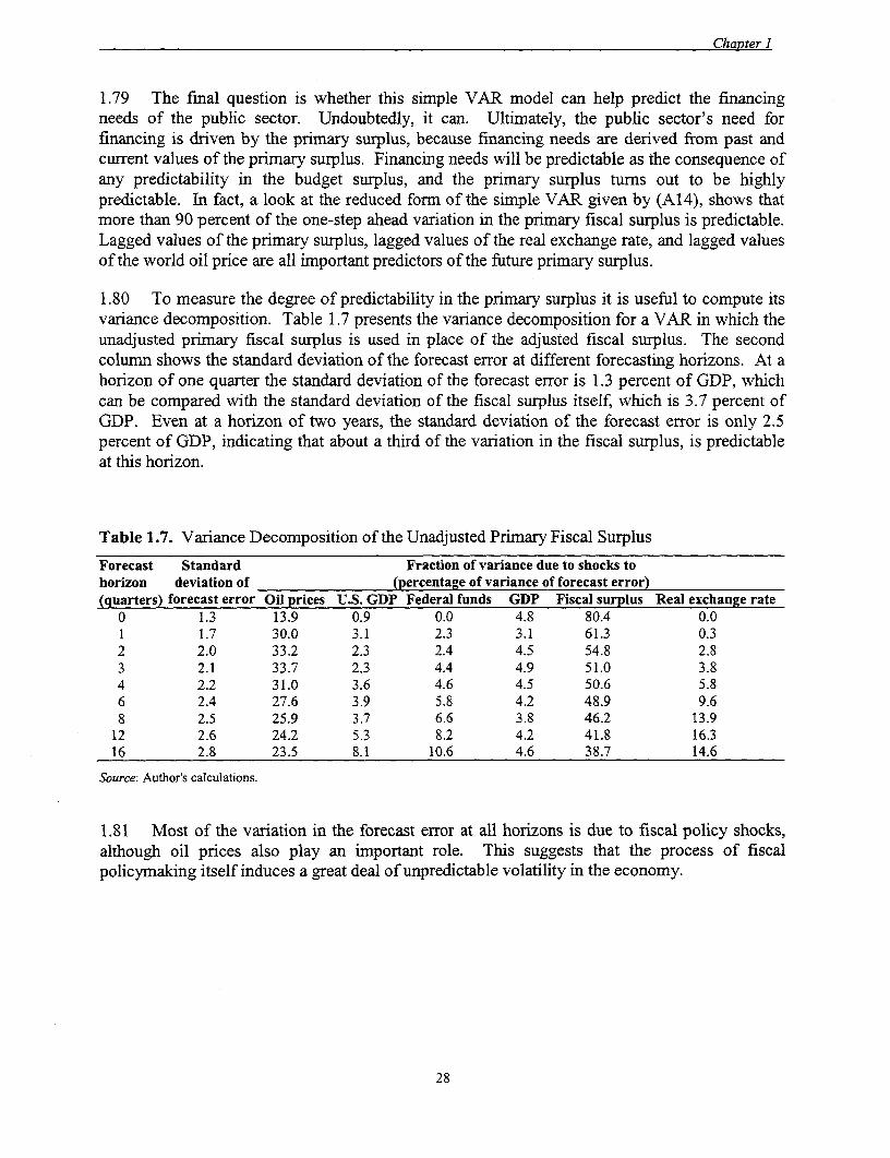
Chapter 1
1.79 The final question is whether this simple VAR model can help predict the financingneeds of the public sector. Undoubtedly, it can. Ultimately, the public sector's need forfinancing is driven by the primary surplus, because financing needs are derived from past andcurrent values of the primary surplus. Financing needs will be predictable as the consequence ofany predictability in the budget surplus, and the primary surplus turns out to be highlypredictable. In fact, a look at the reduced form of the simple VAR given by (A14), shows thatmore than 90 percent of the one-step ahead variation in the primary fiscal surplus is predictable.Lagged values of the primary surplus, lagged values of the real exchange rate, and lagged valuesof the world oil price are all important predictors of the future primary surplus.
1.80 To measure the degree of predictability in the primary surplus it is useful to compute itsvariance decomposition. Table 1.7 presents the variance decomposition for a VAR in which theunadjusted primary fiscal surplus is used in place of the adjusted fiscal surplus. The secondcolumn shows the standard deviation of the forecast error at different forecasting horizons. At ahorizon of one quarter the standard deviation of the forecast error is 1.3 percent of GDP, whichcan be compared with the standard deviation of the fiscal surplus itself, which is 3.7 percent ofGDP. Even at a horizon of two years, the standard deviation of the forecast error is only 2.5percent of GDP, indicating that about a third of the variation in the fiscal surplus, is predictableat this horizon.
Table 1.7. Variance Decomposition of the Unadjusted Primary Fiscal Surplus
Forecast Standard Fraction of variance due to shocks tohorizon deviation of (percentage of variance of forecast error)(quarters) forecast error Oil prices U.S. GDP Federal funds GDP Fiscal surplus Real exchange rate
0 1.3 13.9 0.9 0.0 4.8 80.4 0.01 1.7 30.0 3.1 2.3 3.1 61.3 0.32 2.0 33.2 2.3 2.4 4.5 54.8 2.83 2.1 33.7 2.3 4.4 4.9 51.0 3.84 2.2 31.0 3.6 4.6 4.5 50.6 5.86 2.4 27.6 3.9 5.8 4.2 48.9 9.68 2.5 25.9 3.7 6.6 3.8 46.2 13.9
12 2.6 24.2 5.3 8.2 4.2 41.8 16.316 2.8 23.5 8.1 10.6 4.6 38.7 14.6
Source: Author's calculations.
1.81 Most of the variation in the forecast error at all horizons is due to fiscal policy shocks,although oil prices also play an important role. This suggests that the process of fiscalpolicymaking itself induces a great deal of unpredictable volatility in the economy.
28

Chapter I
Policy Conclusions
1.82 The following subsections highlight the main findings of this chapter and explain whythey are important to policymakers.
Fiscal Policy Is Procyclical
1.83 Mexico's fiscal policy tends to be procyclical. In this way, Mexico resembles manycountries in Latin America. Procyclical policy appears to exacerbate business cycle fluctuations.This begs the question as to how and why fiscal policy behaves in this way.
Automatic Stabilizers Are Weak
1.84 In most of the OECD, taxes and social programs act as natural stabilizers of the businesscycle. Tax revenue, and, in some cases, even marginal tax rates, tend to accelerate duringcyclical upturns. Spending on social programs such as unemployment insurance and welfareincreases during cyclical downturns. These factors tend to make the fiscal surplus move with thebusiness cycle, so that fiscal policy has a natural, and automatic, tendency to dampen businesscycle fluctuations. However, in Mexico these automatic stabilizers are weak. While income taxrevenue, taxes on imports, and VAT revenue all move procyclically, they represent only afraction of the public sector's revenue. Much of this revenue-ultimately about a third of publicsector revenue-comes from petroleum, and this revenue is, if anything, countercyclical.
1.85 Transfer payments appear to be neutral with respect to the business cycle. This isprobably due to the small fraction of transfer payments that is dedicated to social assistance typespending.
Discretionary Policy Is Strongly Procyclical
1.86 Not only are automatic stabilizers weak in Mexico, but the rest of the budget has tendedto be strongly procyclical. Cyclical upturns are an opportunity to expand public sectorinvestment and other forms of discretionary spending. Cyclical downturns bring austerity.However, these effects only exacerbate the business cycle. This chapter has presented evidencethat the discretionary component of policy may have become less destabilizing since the early1990s.
Is Procyclical Policy Really a Problem?
1.87 Procyclical policy makes business cycles more severe. In Latin Arnerican countries itimposes high financing costs as periods of expansion end and recessions begin. As Gavin andothers (1996) point out, international credit dries up when investors recognize that anindustrializing economy is entering a recession. Whether this is exogenous behavior by investorsor not is irrelevant. The fact remains that a recession makes financing a given level of debt moredifficult, so entering a recession with a relatively high level of debt and then having to pay ahigher price for that debt is extremely detrimental to the economy. This is what drives the fiscalcorrections that must be made during recessions. Furthermore, it is what limits the government'sability to shelter the economy's most vulnerable members during bad times.
29

Chapter I
What Can Be Done?
1.88 Automatic stabilizers can be improved. Part of the problem in Mexico is that a third ofall revenue comes from petroleum in one formn or another, and oil prices have tended to becountercyclical. A decreased reliance on oil revenue would be helpful, as would more broadlytargeted taxation of economic activity. Transfer programs could be more narrowly targeted tosoften the blow of cyclical fluctuations.
1.89 Mexico could also improve its discretionary fiscal policy. Discretionary spending,especially public investment, is highly volatile and highly sensitive to the business cycle. Thissuggests that the planning of projects and financing of public expenditure could be bettermanaged so as to smooth it more evenly over time. A commitment to discretionary policies thatlead to larger surpluses during recessions would help the government smooth its financing needs.
1.90 The government could try to smooth its financing needs by smoothing its use of oilrevenues. Interestingly, during the period studied in this chapter (1980-98), oil revenue has been,if anything, countercyclical, so it has been a relatively stabilizing feature of the budget.
1.91 Finally, the government can project its financing needs. Projections of financing over themedium term, along with economic forecasts, should allow the government to manage fiscalpolicy in such a way that a fiscal crunch does not always coincide with a cyclical downturn.
30
Chapter I
References
Beveridge, Stephen, and Charles R. Nelson. 1981. "A New Approach to the Decomposition ofEconomic Time Series into Permanent and Transitory Components with Particular Attentionto Measurement of the 'Business Cycle'." Journal of Monetary Economics 7(March): 151-74.
Blanchard, Olivier. 1990. "Suggestions for a New Set of Fiscal Indicators." Working Paper no.79. OECD Department of Economics and Statistics. Paris.
Brown, E. Cary. 1956. "Fiscal Policy in the Thirties: A Reappraisal." American EconomicReview 46 (December): 857-79.
Buiter, Willem H. 1993. "Measurement of the Public Sector Deficit and Its Implications forPolicy Evaluation and Design." in Mario I. Blejer and Adrienne Cheasty, eds., How toMeasure the Fiscal Deficit. Washington, D.C.: International Monetary Fund.
Chand, Sheetal K. 1993. "Fiscal Impulse Measures and Their Fiscal Impact." in Mario I. Blejerand Adrienne Cheasty, eds., How to Measure the Fiscal Deficit, Washington, D.C.:International Monetary Fund.
Chouraqui, J. C., R. Hagemann, and N. Sartor. 1990. "Indicators of Fiscal Policy: AReexamination." Working Paper no. 78. OECD Department of Economics and Statistics.Paris.
Christiano, Lawrence J., Martin Eichenbaum, and Charles L. Evans. 1998. "Monetary PolicyShocks: What Have We Learned and to What End?" Working Paper no. 6400. NationalBureau for Economic Research, Cambridge, Mass.
de Leeuw, Frank, and Thomas M. Holloway. 1982. "The High-Employment Budget: Revisedand Automatic Inflation Effects." Survey of Current Business 62 (April): 21-33.
. 1983. "Cyclical Adjustment of the Federal Budget and Federal Debt." Survey of CurrentBusiness 63 (December): 25-40.
de Leeuw, Frank, Thomas M. Holloway, Darwin G. Johnson, David S. McClain, and Charles A.Waite. 1980. "The High Employment Budget: New Estimates, 1955-80." Survey of CurrentBusiness 60 (November): 13-43.
EC (European Community), Directorate-General for Economic and Financial Affairs. 1995."Technical Note: The Commission Services' Method for the Cyclical Adjustment ofGovernment Budget Balances." European Economy (60): 35-88.
Fellner, William. 1982. "The High-Employment Budget and Potential Output-A Critique."Survey of Current Business 62 (November): 25-33.
31

Chapter I
Gavin, Michael, Ricardo Hausmann, Roberto Perotti, and Emesto Talvi. 1996. "Managing FiscalPolicy in Latin America and the Caribbean: Volatility, Procyclicality, and LimitedCreditworthiness." Working Paper no. 326. Inter-American Development Bank, Office of theChief Economist, Washington, D.C.
Giomo, Claude, Pete Richardson, Deborah Roseveare, and Paul van den Noord. 1995."Estimating Potential Output, Output Gaps, and Structural Budget Balances." Working PaperNo. 152. OECD Department of Economics, Paris.
Hodrick, Robert J., and Edward C. Prescott. 1997. "Postwar U.S. Business Cycles: An EmpiricalInvestigation." Journal of Money, Credit and Banking 29: 1-16.
Holloway, Thomas M. 1984. "Cyclical Adjustment of the Federal Budget and Federal Debt:Detailed Methodology and Estimates." Bureau of Economic Analysis Staff Paper 40. U.S.Department of Commerce, Washington, D.C.
IIMF (International Monetary Fund). 1993. "Structural Budget Indicators for the Major IndustrialCountries." World Economic Outlook (October): 99-103.
Newey, Whitney K., and Kenneth D. West. 1987. "A Simple, Positive Semi-Definite,Heteroskedasticity and Autocorrelation Consistent Covariance Matrix." Econometrica 55:703-708.
Price, W. R., and P. Muller. 1994. "Structural Budget Indicators and the Interpretation of FiscalPolicy Stance in OECD Economies." OECD Economic Studies (Autumn).
32
Appendix
Alternative Definitions of the Trend in GDP
AL.1 POTENTIAL OUTPUT. The level of potential output is typically defined as the level ofoutput that could be produced if the economy was at full employment or was at the natural rateof employment. The IMF and OECD measures of the cyclically adjusted budget surplus areultimately based on some measure of potential output. Potential output is usually constructedwith reference to some production function that determines GDP as a function of the levels ofcapital and labor in the economy. Suppose output, Y, , is written as a function Y, = f (K,, N, A,)
of the levels of capital, Kt, labor, Nt, and technology, A,. Then potential output is given by
Y = f (KI, N, A,), where N1 is the level of full or natural employment and A, is the trend
level of technology. Making the concept of potential output operational is difficult because itrequires a measure of capital. An annual series on the capital stock is available for Mexico, butideally, some estimate of capital services that took variable utilization into account would beused. Furthermore, the parameters of the production function, f () , must be estimated. Becausetechnology is unobservable, these estimates must be used to decompose fluctuations in outputaccording to their sources: fluctuations in capital, labor, and technology. Finally, the level of fullor natural employment and the trend level of technology must be estimated. Generally speaking,practitioners cannot agree on how to define full or natural employment. For these reasons, theconcept of potential output is not used here.
A1.2 PIECEWISE LINEAR TREND. Figure l.AI(a) illustrates a piecewise linear trend fitted toreal GDP, with a breakpoint at 1988Q1 (first quarter of 1988), the date at which thegovernment's stabilization program was implemented. As table l.Al shows, the break in thetrend is significant at approximately the 5 percent significance level.
33

Figure 1.A1. Trends in Real GDP
(a) Piecewise Linear (b) Hodrick-Prescon
1500 - 1500
° 1400 - 1400-
, 1300 - 1300 -
-1200 -1200-
900 900
80 82 84 86 8 8 90 92 94 96 98 80 82 84 86 8 8 90 92 94 96 98
(c) Beveridge-Nelson (d) Peak-to Peak
1500 - 1500 -. I
°1400 - PK °1400 -
c1300 -N 1300 -5a/
1100 - 1100-
1000 1000
900 900
80 82 84 86 88 90 92 94 96 98 80 82 84 86 88 90 92 94 96 98
Sources: Author's calculations.
Table 1A c Estimates of a Piecewise Linear Trend in the Logarithm of Seasonally AdjustedReal GDP
Coefficient Standard error t-statistic
Constant 13.8 0.051 269
Post-1988 dummy -0.155 0.083 -1.87
Trend 0.0017 0.0023 0.75
Trend x post-1988 dummy 0.0052 0.0027 1.95
Nvote: The estimates were computed using ordinary least squares. The standard errors and t-statistics are robust to
heteroskedasticity and serial correlation. A Newey and West (1987) estimator with five lags was used to compute the
standard errors.
Source: Author's calculations.
A1.3 The deviations fom trend implied by the piecewise linear trend are illustrated in figurel.A2(a). GDP was below trend during the troughs of each of the recessions, as well as at theverCobeginnings ofthe 1980 and 1989-94 expansions.
34
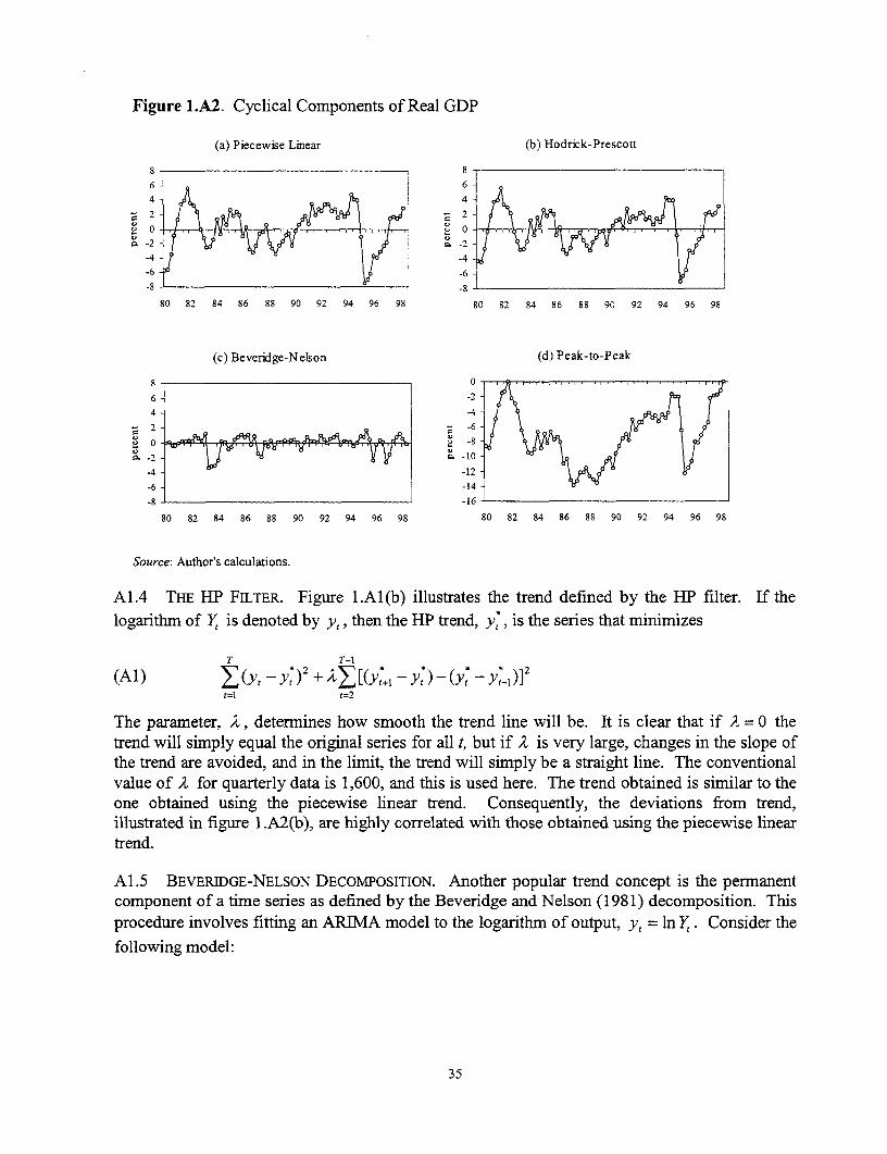
Figure 1.A2. Cyclical Components of Real GDP
(a) Piecewise Linear (b) Hodrick-Prescott
8 -86 - 64 -4
C)(c Beeig-elo d ea-oPa8 0
. -2 , . -2-4 -4
-6 -6
-8 ~~~~~~~~~~~~~~~~~~~~-880 82 84 86 88 90 92 94 96 98 80 82 84 86 88 90 92 94 96 98
(c) Beveridae-Nelson (d) Peak-to-Peak
0
6 -- 2 -
4 -- 4 -
- 2 -- 6-C) 0 ~~~~~~~~~~~~~~~~~~ ~~-8
-2 - -10 d-4 -- 12-
-6 -- 14-
-8 -16
80 82 84 86 88 90 92 94 96 98 80 82 84 86 88 90 92 94 96 98
Source: Author's calculations.
trend will simply equal the original series for all t, but if 2 is very large, changes in the slope ofthe trend are avoided, and in the limit, the trend will simply be a straight line. The conventionalvalue of 2 for quarterly data is 1,600, and this is used here. The trend obtained is similar to theone obtained using the piecewise linear trend. Consequently, the deviations from trend,illustrated in figure .A2(b), are highly correlated with those obtained using the piecewise lineartrend.
A1.5 BEVERIDGE-NELSON DECOMPOSITION. Another popular trend concept is the permanentcomponent of a time series as defined by the Beveridge and Nelson (1981) decomposition. Thisprocedure involves fitting an ARIMA model to the logarithm of output, y, = In Y, . Consider the
following model:
35

(A2) Ayt - u = a, (yt-I - p) + a2 (YI-2 -i) + A + ap (y, p - ,u) + ,
where u is the mean of Ayt. The permanent component of y., yt , is given by its current value
plus any predicted stochastic growth in the series:
(A3) Yt = Yt + Et (yt+l - u) + Et (Yt+ 2 -u) + A.
A1.6 An estimate of the perrnanent component can be obtained by estimating equation (A2)and using it to compute the expectations on the right-hand side of equation (A3). Here, equation(A2) was estimated using maximum likelihood, and the order of the autoregression, p, waschosen according to the Schwartz criterion, which selected p = 2. The resulting trend estimatesare plotted in figure l.Al(c). The deviations from trend are plotted in figure l.A2(c). The mostnotable aspect of the trend is that it closely tracks the original series. The deviations from trendare much smaller, and they behave differently than those identified using the piecewise lineartrend and the HP filter. They are typically most negative during the early part of cyclical upturnsand most positive at the end of expansions. Thus they appear to be more useful as indicators ofcyclical turning points than as indicators of the cycle itself. For this reason, the Beveridge-Nelson procedure is not used here.
A1.7 PEAK-TO-PEAK TREND. Finally, an ad hoc procedure that is sometimes used is to draw apeak-to-peak trend line so that observed output is never above the trend. In this case, a lineartrend in the logarithm of Y, was used to connect the peaks in 1981Q4 and 1998Q2 as illustrated
in figure .AlA(d). With the trend specified in this way, output never lies above the trend. Thedeviations from trend are plotted in figure l.A2(d). They are highly correlated with thedeviations from trend defined by the HP filter and the piecewise linear trend, with correlationcoefficients of 0.78 and 0.73, respectively. Given the high correlation with the other measures,and the ad hoc nature of the peak-to-peak trend, the cycle defined in this way is not used here.
Alternative Definitions of the Cyclical Component of the Budget
A1.8 The baseline method of adjustment used in this chapter follows the methodology of theEC fairly closely. First, a limited number of expenditure and revenue categories are selected foradjustment. To illustrate the method of adjustment, take as an example personal income taxrevenue, 7Y, one of the revenue categories that is usually adjusted. Its elasticity with respect to
output, eTY is given by
(A4) eTy = aln( )
A1.9 The elasticity might be estimated using a purely statistical model of the relationshipbetween income tax revenue and GDP. It could also be obtained with reference to statutory taxrates, and a statistical model of the relationship between personal income and GDP, as in themethod employed by the Bureau of Economic Analysis of the U.S Department of Commerce,discussed below.
36

Al.10 In this chapter estimates of the elasticities of various revenue and expenditure categorieswith respect to the output gap were obtained using the following statistical model, illustrated inthe case of income taxes:
(A5) t = eTYy + E,t
where rTy, and y' represent the cyclical components of income taxes and output, respectively, as
measured using the HP filter.
Al.11 Given an estimate of the elasticity, the EC method adjusts income tax revenue by theamount
(A6) - g [eXp(eTYyt )- 1]
where y' is the cyclical component of output in logarithmic percentage terms. If the cyclical
component is zero, clearly no adjustment to tax revenue is made. If the cyclical component ispositive and the elasticity is positive, then the adjustment will be negative. This makes intuitivesense: during a cyclical upturn tax revenues rise simply because the economy is expanding. Toadjust for this effect, tax revenue should be adjusted downward.
A1.12 In general, with a method such as this the adjusted budget surplus is easy to compute.Any standard budget surplus measure, A, is defined as the difference between revenue, Rt, and
expenditure, X,. To adjust the budget surplus for the business cycle and create a new budget
surplus measure denoted A, one uses data on the cyclical component of output, y', along withestimates of the revenue and expenditure elasticities. Suppose there are N revenue categories,{Rl......,RJ} and M expenditure categories, {X,,..., Xm }, to be adjusted. Suppose the
elasticity of R it with respect to output is given by eR1, while the elasticity of Xj, with respect to
output is given by exi I The adjusted surplus measure is given by
At = A, + adjustment
(A7) = (Rt X, ) - R[exp(eRjy' ) i]-E Xjj [exp(exyu )-lj=1 j=,
A1.13 The Bureau of Economic Analysis (BEA) of the U.S. Department of Commerce has aconcept of the budget surplus, which was originally described as a high employment budgetsurplus. It is described in numerous papers, and attempts to compute the budget surplus thatwould prevail were the economy at full employment and discretionary policies were unchanged.(See, for example, de Leeuw and Holloway 1982, 1983; de Leeuw and others 1980; andHolloway 1984). Later variants make adjustments for the effects of inflation on the budgetsurplus, via its effects on interest expenditure and indexed transfer programs.
Al.14 The BEA's approach is relatively complicated and involves going through the budgetcomponent by component making individual adjustments. For example, to compute adjusted
37

personal income taxes, the adjustment procedure first asks what personal income would be at fullemployment. It denotes this level of income as yp and the actual level of personal income as Yp .
To compute Yp the method proposed involves estimating the elasticity of changes in Yp withrespect to changes in the output gap, which is the difference between actual output and potentialoutput. Roughly speaking, the estimated Yp adds to Y. that elasticity times the measured outputgap. The adjustment process also recognizes that personal taxes are not unit elastic with respectto personal income. In other words, when personal income rises by 1 percent, personal taxesmay rise by some different amount, say e percent. So adjusted personal tax receipts, Tp , will begiven by
(A8)
where Tp represents actual personal tax receipts.
Al .15 The BEA method presents a number of difficulties in the Mexican context. First, ratherthan directly relating each revenue and expenditure category to the output gap, it relates themindirectly. In the example, personal taxes are related to personal income, which is then related tothe output gap. For Mexico, measuring the relevant income concepts would add a difficult layerof complexity. In addition, the output gap concept requires the assessment of potential output,which is a difficult task even for the United States. Fellner (1982) has argued that the potentialoutput concept is not useful, because true potential output depends on a number of unobservablesthat are not involved in its estimation. The BEA method sets potential output equal to what isreferred to as middle-expansion trend gross national production, or gross national product at thenatural rate of unemployment (see de Leeuw and Holloway 1983 for the methods used tocompute these concepts of potential output). For these reasons a simpler method is adopted here.
A1.16 The IMF and OECD methods resemble each other and are described in some detail inIMF (1993) and Giorno and others (1995). Like the BEA method, they both require obtaining anestimate of potential output. Suppose that output is given by a function of capital, labor, andtechnology, and suppose further that this function takes the Cobb-Douglas form:
(A9) Y, = AtK aNI-a
where the notation is defined as before. Then potential output is given by
(A1O) Y' = A;K, (N; a
where N, is the natural level of employment and A, is the trend level of technology. Generallyspeaking, the IMF and OECD measures of potential output are derived by first estimatingequation (A5) and obtaining estimates of the level of technology, A,. The HP filter-based trend
38

of the series A, is generally used to define A; . The OECD computes the natural level of
employment using a model of unemployment rates consistent with nonaccelerating inflation,while the IMF method uses unemployment rates defined by the HP trend in observedunemployment to define natural employment. Both methods use estimates of the actual capitalstock in estimating potential output.
A1.17 Once the estimate of potential output is obtained, the method for estimating the cyclicaladjustments is similar to the one described in the main text. In particular, on the revenue side theEC and OECD make adjustments to corporate taxes, personal income taxes, social security taxes,and indirect taxes. On the expenditure side, the EC and the OECD make an adjustment that ismore complicated, and only adjusts for the effects of the business cycle on unemploymentbenefits. They use a model linking the output gap to the unemployment rate, and hence to thelevel of unemployment benefits. All other expenditure categories are assumed to bediscretionary.
Details of the VAR Model
Al .18 The VAR is defined in terms of z, = (pO, Yu ru, . YMt St) s. A structural VAR
model for z1 that permits contemporaneous feedback between the variables is given by
(Al1) Bzt = A(L)z,-l + st
where B is a nonsingular square matrix, A(L) is a kth-ordered polynomial in the lag operator,
and s, is a vector of mutually orthogonal serially uncorrelated shocks. Premultiplying (Al 1) by
B-1 one obtains
(A12) z, = C(L)zt, + ut
where C(L) = B-'A(L) is a kth-ordered polynomial in the lag operator and u, = B-K1s is a vector
of potentially correlated error terms. The standard procedure for estimating VARs is to choose k,and then simply run ordinary least squares regressions for each equation implicit in (A12). Thecovariance matrix of the residuals from these ordinary least squares regressions, along with a setof identifying restrictions on B, is used to estimate B.
Al.19 The procedure used here is nonstandard in that it imposes zero restrictions on variousparts of A(L) as well as of B. Specifically, because one could argue that the world oil price is
determined strictly exogenously with respect to the other variables in zt, it is assumed that thefirst equation in (Al 1) is given by
(A13) Pot = All]Po1 l + A12po0 -2 +***+ A1kIP0-k +61t
39

A1.20 One could further argue that U.S. real GDP and the U.S. Federal Funds rate aredetermined exogenously with respect to the last three variables in zr.. Furthermore, Christiano,Eichenbaum, and Evans (1998) assume that the U.S. Federal Reserve observes enoughinformation on the U.S. economy that the Federal Funds rate should feed back oncontemporaneous output, but not enough for the reverse to occur. Hence it is assumed here thatthe next two equations in (Al1) can be represented as
(A14) Yu. =-B2 p + (X2, A 2 A(3A)zA A + A + (A'1 Ak2 Ak3)zl,k +
and
(A15) rut =B 3 p- -B3 2 y +(A31 A[2 A13)z,,,+A +(A 1 A 2 Ak )zltk + 3,
where zlt = (ot YUt rut) mutually orthogonal shocks to the six variables.
A1.21 The rest of the VAR is standard. The identifying assumptions imposed on the remainingequations are as follows. The cyclically-adjusted fiscal surplus is assumed to feed backcontemporaneously on the external variables, that is z,,; the level of GDP is assumed to feedback contemporaneously on the external variables and the fiscal surplus; and finally, the realexchange rate is assumed to be determined by contemporaneous feedback from all the othervariables. This implies that B has the usual lower triangular form with ones on the diagonal.
Al.22 With these identifying assumptions the model can be estimated equation by equationusing ordinary least squares. The analysis in the main text was conducted using data that hadbeen HP filtered. This is inappropriate in the context of a VAR model, because a simpleautoregression cannot, by construction, whiten the data.' For this reason, the VAR analysis inthis section is conducted under the assumption that each of the time series in the VAR has alinear deterministic trend (or no trend at all). This allows the VAR to be estimated in levels, witha trend included on the right-hand side.
1. The HP filter is an approximately asymmetric double-sided filter. Thus each observation consists of a doublesided moving average of whatever the true serially uncorrelated innovations in the data are. Given this, anautoregression defined over HP filtered data can never have a serially uncorrelated error as equation (A7)assumes.
40

INFRASTRUCTURE, EXTERNAL SHOCKS,AND MEXICO's FIscAL AccOUNTS
2.1 This chapter develops a dynamic general equilibrium model to analyze issues of stability inthe Mexican economy. It focuses on whether increased provision of infrastructure can reduce theimpact of exogenous shocks on the real economy. That is, would the impact of a shock be less ifhigher levels of infrastructure spending were in place at the time of the shock?
2.2 The answer to this question is a qualified yes. All else being equal, higher stocks ofinfrastructure will tend to reduce the declines in real income caused by certain types of shocks. Wereach this conclusion by carrying out a series of numerical exercises based on a model thatincorporates various types of estimated Mexican data. The model incorporates four types ofinfrastructure in the production process: electricity, telecommunications, transportation, andeducation. In general, the estimates indicate that in Mexico, increased provision of infrastructure,either by the public or private sector, tends to be cost reducing.
2.3 Using a variety of Mexican data sources, we calibrate our model to the years 1995-97 as partof a six year simulation for the years 1995-2000. We subject the model to two types of shocks. Thefirst is a shock to the interest elasticity of money demand that causes the absolute value of theelasticity to decline. Such a shock might be caused by a sudden loss of confidence in the bankingsystem, and tends to increase holdings of money and reduce bank deposits. Over time, this shockbrings about an increase in the real interest rate, a deflation, and a reduction in real gross domesticproduct (GDP) amounting an annual average of about half a percentage points over the six years ofthe simulation.
2.4 We then suppose that prior to the shock infrastructure spending was higher, in real terms, oneach of the four types of infrastructure. The increased provision of infrastructure reduces privatesector costs and, as a result, real GDP rises to a somewhat higher level than in the initial preshocksimulation. We thus conclude that higher levels of infrastructure stocks can indeed insulate theMexican economy from certain types of shocks.
2.5 The second shock is an external shock: stagnation of the world's real income for the sixyears of the simulation. This lowers the demand for Mexican exports and, accordingly, the rate ofgrowth of real Mexican income. In this case, as before, a higher level of expenditure oninfrastructure before the shock and throughout the period of the simulation tends to neutralize theimpact of the shock on real Mexican income. We therefore conclude that the positive implications
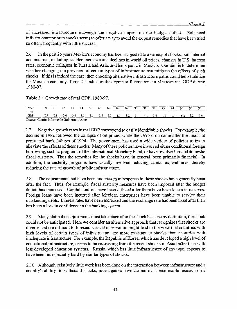
Chapter 2
of increased infrastructure outweigh the negative impact on the budget deficit. Enhancedinfrastructure prior to shocks seems to offer a way to avoid the ex post remedies that have been triedso often, frequently with little success.
2.6 In the past 25 years Mexico's economyhas been subjected to a variety of shocks, both internaland external, including sudden increases and declines in world oil prices, changes in U.S. interestrates, economic collapses in Russia and Asia, and bank panic in Mexico. Our aim is to determinewhether changing the provision of certain types of infrastructure can mitigate the effects of suchshocks. If this is indeed the case, then choosing alternative infrastructure paths could help stabilizethe Mexican economy. Table 2.1 indicates the degree of fluctuations in Mexican real GDP during1980-97.
Table 2.1 Growth rate of real GDP, 1980-97.
Year 80 81 82 83 84 85 86 87 88 89 90 91 92 93 94 95 96 97ReaiGDP 8.4 8.8 -0.6 -0.4 3.6 2.6 -3.8 1.5 1.1 3.2 5.1 4.3 3.6 1.9 4.4 -6.2 5.2 7.0
Source: Cuarto Informe de Gobierno, Annex.
2.7 Negative growth rates in real GDP correspond to easily identifiable shocks. For example, thedecline in 1982 followed the collapse of oil prices, while the 1995 drop came after the financialpanic and bank failures of 1994. The governmnent has used a wide variety of policies to try toalleviate the effects of these shocks. Many of these policies have involved either conditional foreignborrowing, such as programs of the International Monetary Fund, or have revolved around domesticfiscal austerity. Thus the remedies for the shocks have, in general, been primarily financial. Inaddition, the austerity programs have usually involved reducing capital expenditures, therebyreducing the rate of growth of public infrastructure.
2.8 The adjustments that have been undertaken in response to these shocks have generally beenafter the fact. Thus, for example, fiscal austerity measures have been imposed after the budgetdeficit has increased. Capital controls have been utilized after there have been losses in reserves.Foreign loans have been incurred after Mexican enterprises have been unable to service theiroutstanding debts. hiterest rates have been increased and the exchange rate has been fixed after theirhas been a loss in confidence in the banking system.
2.9 Many claim that adjustments must take place after the shock because by definition, the shockcould not be anticipated. Here we consider an alternative approach that recognizes that shocks arediverse and are difficult to foresee. Casual observation might lead to the view that countries withhigh levels of certain types of infrastructure are more resistant to shocks than countries withinadequate infrastructure. For example, the Republic of Korea, which has developed a high level ofeducational infrastructure, seems to be recovering from the recent shocks in Asia better than withless developed education systems. Russia, which has little infrastructure of any type, appears tohave been hit especially hard by similar types of shocks.
2.10 Although relatively little work has been done on the interaction between infrastructure and acountry's ability to withstand shocks, investigators have carried out considerable research on a
42

Chapter 2
related topic, that is the relationship infrastructure provision and a country's rate of real growth.Aschauer (1997) carries out an analysis of a broad range of countries. Among a variety of policies,he considers the impact on economic growth of an increase in public capital, financed by a reductionin government consumption. He finds that the impact of a shift of government expenditure equal toone standard deviation of the sample distribution for public investmnent is, on average, 2.15. In thecase of Mexico, the relevant elasticity is 2.20. Given the structure of the estimates, this would meanthat an increase in public investment by 63 percent of actual output would lead to an increase in theaverage annual growth rate of about 0.6 percent. These magnitudes are quite close to those generatedby our simulations, even though ours are generated by a general equilibrium framework while thesecome from a partial equilibrium analysis. Note also that Mexico lies at approximately the middle ofthe group of 46 sample countries. Uruguay had the highest estimated elasticity, 5.04, while Algeriahad the lowest, 0.38.
2.11 One might suppose that not all types of infrastructure are equal. Thus, for example, having anextensive network of roads might have less of an impact on a country's ability to sustain shocks thanhaving a well-educated populace. At the same time, infrastructure might have different impacts ondifferent sectors of the economy. For instance, what might protect manufacturing from, for example,an oil price shock, might do little for agriculture.
2.12 We therefore construct a dynamic model that incorporates an arbitrary number of types ofinfrastructure. These different types of infrastructure will have varying impacts on the differentsectors of the economy. The next section discusses the Mexican background to our analysis. Thefollowing section develops the analytical model. Next we discuss data sources and simulation resultsobtained from the model using Mexican data, before summarizing our findings and reaching aconclusion.
Background
2.13 A variety of reasons exist for reducing infrastructure expenditures. Governments oftendetermine that the easiest way to reduce public expenditure is to cut capital spending. They feel theydo not need to cut public payrolls drastically, as would be the case if they reduced civil serviceemployment or wages. The costs, if any, of reduc ed formation of infrastructure are usually not feltfor some time. Mexico is an extreme case of government reduction in public investment. Publicinvestment fell from 12.1 percent of GDP in 1981 to 4.2 percent of GDP in 1989. At the same timeeconomic growth slowed down markedly. Real GDP, which grew by 8.8 percent in 1981, grew byonly 1.1 percent in 1988, while private investment remained approximately constant as a percentageof GDP.
2.14 Drawing conclusions from a category as broad as public capital formation is, of course,difficult. Table 2.2 shows the stock of capital in three key types of infrastructure: electricity and gas,transportation, and communications. The rates of growth of all three changed drastically during1970-90. For example, from 1970 to 1980 the stock of capital in electricity and gas grew by 12.8percent per year. From 1980 to 1990 the corresponding rate of growth was only 0.3 percent per year,and the stock of electricity and gas infrastructure declined from 1981 to 1990. The stock of capital in
43

Chapter 2
transportation grew by 8.7 percent from 1970 to 1980, but only by 3.5 percent from 1980 to 1990.Similarly, communications capital grew by 49.8 percent per year from 1970 to 1980 and by 4.1percent from 1980 to 1990.
Table 2.2. Stocks of Infrastructure, 1970-90(millions of pesos at constant prices)
Year Electricity and Gas Transportation Communications1970 19013.1 9062.5 147.81971 22285.4 9562.9 153.61972 26091.1 9863.7 180.71973 30141.8 10066.8 218.21974 33986.5 10045.8 248.31975 37846.9 12244.8 1398.71976 44798.6 17055.9 3658.41977 46669.3 18495.8 5524.51978 51148.1 19536.6 7458.91979 55761.8 20368.6 9137.71980 63419.0 20921.4 8436.31981 70175.4 22809.5 10342.31982 73962.6 23875.1 11124.01983 73587.9 24511.5 11276.71984 71613.8 24630.4 11818.71985 69216.9 25213.3 12471.31986 66555.8 25096.6 11689.61987 64195.5 26583.0 11975.31988 65630.1 31746.4 13409.71989 65340.5 30763.4 12769.11990 65110.6 29372.1 12564.5
Source: La Encuesta de Acervos, Depreciaci6n y Formaci6n de Capital del Banco de Mexico.
2.15 Feltenstein and Ha (1998) develop a two-period model that analyzes the extent to whichinadequate levels of public infrastructure have contributed to slow economic growth in Mexico.Feltenstein and Ha (1995) use a partial equilibrium model to estimate the income shortfall due to thedecline in the stock of Mexican infrastructure. Infrastructure may be either publicly or privatelyprovided. If the infrastructure is publicly provided, as was the case in Mexico until 1990, thenchanges in its rate of provision will effect the government's budget deficit, with correspondingchanges in the domestic interest rate. For example, an increase in the public provision ofinfrastructure may, initially, increase the productivity of private capital, leading to increases inoutput. The rise in interest rates caused by larger budget deficits may, however, dampen privateinvestrnent, leading to a less than expected eventual increase in private output.
2.16 Here we develop a multi period model that allows us to examine not only the effect of changesin both publicly and privately provided infrastructure on GDP, but also upon the stability of theMexican economy in response to shocks. Relatively little analysis of the relationship between
44

Chapter 2
infrastructure provision and a country's ability to withstand shocks has been carried out for othercountries. Nonetheless, we can make certain comparisons. (Our examples are taken from WorldBank 1998.)
2.17 In Mexico, as in many other countries in Latin America, the decline in real growth in theperiod 1984-94 is closely associated with a decline in total factor productivity. Indeed, about 2/3 ofthe decline in the rate of growth of Mexico's per capita real income may be explained by the declinein total factor productivity. The remaining portion of the decline comes from the slow down incapital accumulation. Although physical capital accumulation slowed during this period in Mexico,educational achievement continued to rise, in contrast to most of the other countries in LatinAmerica.
2.18 Evidence concerning Mexico's ability to respond to shocks is mixed. Several studies cited inWorld Bank (1998) note that economic reforms took place essentially after the fact, in much thesame pattern as in most of Latin America. Thus, reforms would be instituted after the shockoccurred, although in the Mexican case, the improvements after the reforms came more slowly thanin many other countries. Chile and Mexico offer a useful comparison. In the early 1980s, Chilesuffered an output collapse similar to that of Mexico. Unlike Mexico, however, Chile had alreadycompleted its trade and financial liberalization programs by the time the shocks occurred. As aresult, Chile's initial collapse was followed by a sustained output recovery. In Mexico, however,measures such as trade liberalization followed after the collapse. Also, Mexico nationalized itsbanking system, thereby reducing savings, and hence private investment, while Chile liberalized itsfinancial system, thereby increasing private savings and, accordingly, the rate of capital formation.
2.19 Along with the failure to carry out financial reformns in advance of the shocks, did Mexico'sfailure to provide adequate rates of growth of infrastructure contribute to the severity of shocks?Using estimated parameters for the entire Mexican economy, in particular, for the elasticities ofoutput with respect to infrastructure, we investigate this issue later. Let us now turn to the model.
Model Structure
2.20 This section analyzes the concepts discussed with the help of a dynamic model designed topermit simulation. The model is based on n discrete time periods. During each period all agentsoptimize over a two-period time horizon. That is, in period t agents optimize given prices for periodst and price expectations for period t + 1, and the future thereafter. When period t + 2 arrives, agentsreoptimize for periods t + 2 and t + 3, based on new information about period t + 2. In particular,after events that take place during the first two periods, shocks may occur. For example, certainsectors in the economy may have become insolvent, leading to bank defaults. Because these defaultswere not anticipated in period t, they cause agents to recalculate the value of their assets as theyoptimize over the next two periods. Alternatively, some external shock could have occurred such asan oil price change, or a foreign interest rate change, that may have implications for the domestic realeconomy.
45

Chapter 2
2.21 The following subsections describe specific details of the model. (See Feltenstein 1992 andFeltenstein and Morris 1990 for the basic structure of production and demand in a perfect foresightcontext.)
Production
2.22 We assume that, in addition to conventional factors, the process of production indirectlyrequires of liquidity, that is, monetary assets, to finance investment. These assets are thereforeimplicitly incorporated as factors in the production function. We assume that domestic productiontakes place in various sectors that use inputs of capital, labor, and land. In addition, infrastructureenters as inputs into private production, possibly as cost-reducing elements. Therefore the productivestructure of the model includes at least three factors of production and three categories of financialassets: domestic currency, bank deposits, and foreign currency. Also, there maybe multiple types ofinfrastructure, some of which are costless to the private producer and some of which requirepayments, for example, publicly provided education maybe free, while privatelyprovided electricityrequires payment. Each of these factors of production, as well as the financial assets, are replicatedin each period and, accordingly, have a price in each period. Domestic currency in period 1 is takenas the numeraire.
2.23 We use an input-output matrix, A,, to determine intermediate and final production in period t.Corresponding to each sector in the input-output matrix, value added is produced using capital, labor,land, and infrastructure' We may now specify the following problem for the firim. Let yKI , YLi be
the inputs of capital and labor to thejth sector in period i (we will ignore land to simplify notation).Let YGi be a vector representing the outstanding stocks of infrastructure of various types in period i.The production of value added in sectorj in period i is then given by
Va1 i = vaii (yK{ , YLi YGI)
Sectorj pays value added taxes on inputs of capital and labor, given by tKij, tLij, respectively, inperiod i.2 Hence the effective price for labor and capital paid by sectorj is
PLY ( + tLY)PLY, PKj (l + tKY)PK#
Thus if P = (IPKi, ILY) are the prices of capital and labor in period i, then the prices of
1. The use of neoclassical value added functions "sitting above" an input-output matrix is conmmon (see Shoven andWhalley 1984 for this approach). An application and a detailed description of functional formrs are given inFeltenstein (1986). Thus, for example, agriculture would use land and labor while manufacturing would use capitaland labor.
2. The interpretation of these taxes is, thus, as a profit tax and a personal income tax that is withheld at the source.
46

Chapter 2
goods charged by enterprises, pi, are given by
(pi) = va (P, YGi) (I + t)(I - A )-'
where va(P, YGd) is the vector of cost-minimizing, value added per unit of output.
2.24 We now suppose that each of the one or more capital types is produced via a sector-specificinvestment technology that uses inputs of capital and labor to produce new capital. Investment iscarried out by the private sector and is entirely financed by domestic borrowing.3Producer's/investor's may receive an investment tax credit as well as a depreciation allowance, andpay a profit tax on the returns to their investments. The appendix provides the specification of theinvestor's problem.
2.25 Investor's take out a loans from the banking system to cover their costs. The operationalassumption is now made that when feasible new investment, as a percentage of the existing sectoralcapital stock, falls below a certain minimum threshold, firns are unable to pay the debt obligations
4that they incurred to finance their capital formation. Accordingly, banks holding these assets nowhold corresponding bad debts. This situation might occur if, unexpectedly during the period, interestrates in the economy rose sufficiently so as to reduce firms' profitable investment below thepredetermined threshold. This assumption implies that each firm has a lower feasibility bound for itsoperations, reflected by its level of investment, below which it cannot operate. This threshold,expressed as a percentage of the existing capital stock, is taken here as exogenously determined, forinstance, by pre-existing technology. We also assume, for simplicity, that the threshold is uniformacross sectors.
3. We assume that all foreign borrowing for investment is carried out by the govemment, so that, implicitly, thegoverniment is borrowing for the private investor, but the debt thereby incurred is publicly guaranteed.
4. It is thus claimed that, as a proxy, a firm whose investments fall below some predetermined rate is, in practice,bankrupt.
47
Chapter 2
Banking
2.26 Without loosening generality, here we simplify the structure of the banking sector. Eachbroad sector of the economy has one bank. To be specific, we will suppose that the economy hasfive such sectors. Each bank lends primarily, but not exclusively, to a certain sector; therefore, banksare potentially, but not fully, specialized. To streamline the simulations, we assume that the assets ofeach bank include 50 percent of the outstanding debt of its particular sector. It then holds 12.5percent of the debt of each of the remaining four sectors.5 This assumption about the diversificationof assets avoids the ease with which the insolvency of a particular sector leads to the automaticinsolvency of its related bank. A solvency requirement is then imposed on individual banks: if 8percent of a bank's assets are in default, caused by a corresponding insolvency of its borrowers, thenthe bank is declared insolvent and is seized by the government. Depositors in the seized bank findtheir assets frozen. Of course, a bank declared insolvent cannot continue to lend.6
2.27 Thus, the bank's supply of loans, and hence its assets determines the demand for loans fromthe productive sectors of the economy. Of course, given the existence of a maximum lending tocapital ratio, that bank's capital restricts its supply of loans. The bank's liabilities (deposits) aredetermined by consumers' savings behavior, which in turn is derived from the intertemporaloptimization of consumption.
Consumption
2.28 We permit an arbitrary number of consumers, each of whom has Cobb-Douglas demandfunctions. The consumers may also differ in their initial allocations of scarce resources and financialassets. The consumers maximize utility functions subject to intertemporal budget constraints-thathave as arguments the levels of consumption and leisure in each of the two periods. The model issimilar to that of a standard cash in advance structure. Consumers save by holding money, bankdeposits, government bonds, and foreign currency. They require money for transactions purposes, buttheir demand for money is sensitive to changes in the interest rate. In addition, the consumers'demand for bank deposits is sensitive to their perception of the solvency of the banking system,reflected in the level of non performing assets in the system. In particular, as banks increasingly incurbad loans, the consumers' interest elasticity of money declines, leading them to reduce their bankdeposits, which reflects the notion that consumers worry about the safety of their deposits as theyperceive banks becoming progressively more insolvent.
5. Clearly these percentages are arbitrary, and should serve only for sinplification and illustrative purposes. Any initialpattem of distribution of bank assets across different sectors will provide results consistent with the hypotheses ofthe chapter.
6. An 8 percent loss of assets would be tantamount to a total liquidation of capital. While other values could be used forthe purpose of the simulation, 8 percent corresponds to intemational standard practices.
48

ChapRter 2
The Government
2.29 The government collects income, profit, and value-added taxes, and import duties. It pays forthe production of infrastructure and public goods, as well as for subsidies. In addition, thegovernment must cover both domestic and foreign interest obligations on public debt. The deficit ofthe central government in period 1, DI, (as before, 1 denotes period i and 2 denotes period i + 1) isthen given by
Di = G1 + Si + ri Bo + rFJ ei BFO - Ti
where SI represents subsidies given in period 1. GI is spending on goods, infrastructure, andservices; while the next two terms reflect domestic and foreign interest obligations of thegovernment based on its initial stocks of debt. TI represents tax revenues.
2.30 The resulting deficit is financed by a combination of monetary expansion, and domestic andforeign borrowing. If AyBGI represents the face value of domestic bonds the government sells inperiod 1 and CFI represents the dollar value of its foreign borrowing, then its budget deficit inperiod2 is given by
D2= G2 + S2 + r2(A YBGI + Bo) +e2rF2(CFl + BFo) -T2
where r2(AyBGI+Bo) represents the interest obligations on its initial domestic debt plus borrowingfrom period 1, and e2rF2(CFL+BFO) is the interest payment on the initial stock of foreign debt plusperiod 1 foreign borrowing.
The Foreign Sector and Exchange Rate Deternination
2.31 The foreign sector is represented by a simple export equation in which aggregate demand forexports is determined by domestic and foreign price indexes and world income. We also permitexogenously determined exports. In the case of Mexico, this would be represented by oil exports,which are not market determined.
2.32 The government also chooses an exchange rate regime. The model permits essentially anyregime, from fixed to floating. In our simulations we will use a modified floating rate. We havetaken foreign lending to be exogenous.7 Thus gross capital inflows are exogenous, but the change inreserves is endogenous. The supply of foreign reserves in period i, yFGi, is given by
YFGi YFG(i-) + Xi Mi + XF(i1) XFi + CFi -
7. Capital inflows in Mexico are, of course, endogenously determined by a variety of factors. We are mnaking asimplifying assumption here, because the determrination of capital flows is not the primary focus of our analysis.
49
Chapter 2
Here xFi represents the demand for foreign assets by citizens of the home country, so XF(i-4) - XFi
represents private capital flows. The govermnent has a demand for foreign assets that is determinedby an exchange rate rule. Let yFi represent whatever the government feels to be the critical level offoreign reserves in period i. The government wishes to peg the exchange rate in period i, ei, at itslevel of the previous period, ei ,,. It will, however, adjust the exchange rate if its stock of reserves,YFGi, deviates from its target, YFi.
Money Supply
2.33 Changes in the money supply in period i, AMs8 , are now given by
A Msi = A ym* + A OMOI + ei YFGi ei- , YFG(i-I)
where Aymlfi is deternined the government financing of its budget deficit, and A OMOi representsmoney created by the central bank via open market operations. The remainder of the right-hand siderepresents the domestic currency value of the external sector balance.
Data Sources, Calibration, and Simulations
2.34 Because our model does not permit an analytical solution, we will use a numerical solutionmethod to derive certain qualitative conclusions about the effect of alternative paths of infrastructuregrowth on stability in the presence of shocks.8 We derive a fixed point that corresponds to anintertemporal equilibrium. This equilibrium thus represents a set of prices in each period at whichall factor and financial markets clear.
2.35 To simulate our model we have used production, demand, export, and migration parameterestimates reported in Feltenstein (1992), Feltenstein and Ha (1995, 1998), Feltenstein and Shah(1995), and Murphy and Feltenstein (1999). We have taken initial allocations to be the stocks at theend of 1994. We carry out a simulation for a six year period representing 1995-2000. All exogenousparameters for the first three years take on values equal to their Mexican values over the period1995-97. We then assume that these parameters maintain the same values for the final 3 years ofthesimulation.
2.36 We wish to use this benchmark case as a reference point for alternative policy simulations.We use a variety of data sources, apart from our estimated parameters. These are as follows:
* There are nine sectors that correspond to Mexican national income accounts, namely,1. agriculture;
8. The solution to the model depends on finding a fixed point for the underlying Arrow-Debreu economy. This fixedpoint does not permit an analytical solution, but depends on an iterative numerical methodology. We use a variant ofMerrill's algorithm to solve the problem.
50

Chapter 2
2. mining and resource extraction;3. manufacturing;4. construction;5. electricity, gas, and water;6. commerce, restaurants, and hotels;7. transport and communications;8. financial and housing services;9. social services.
* Sectoral value added (in real terms) is taken from Estados Unidos Mexicanos (1998, p. 27), for1997. Real value added per unit of final output is fixed, but the shares of factor inputs vary.
2.37 Production functions for value added, incorporating infrastructure are derived from Murphyand Feltenstein (1999). These incorporate estimated elasticities for four types of infrastructure:electricity, transportation, communications, and education. These estimates are based on seeminglyunrelated regression estimates of a two-equation system: sectoral cost and the labor share of totalcosts. Capital and labor shares are computed using the "NIPA" data. Both estimates imposeconstant returns to scale and include dummies for
- Sector- Sector * factor prices- Sector * output- Sector * infrastructure.
2.38 The elasticities are calculated using the sectoral average of the appropriate wage and outputmeasures for the estimation subsample (as opposed to calculating the elasticities for each year usingthat year's sector wage and output and then averaging the elasticities over the estimation period).
The standard errors are calculated using the estimated coefficient variance-covariancematrix and assuming the average wage and output figures are constants. That is, if
b = column vector of infrastructure coefficientsA row vector of "weights" (for example, average wage)V = variance-covariance matrix
then the elasticities (e) are
e=A*b
and
V(e) = A * V(b) * A'.
51

Chapter 2
2.39 Interestingly, almost all the elasticities are relatively small, that is on order of magnitudeof l 0.25 l or so. The electric ones are generally negative, transport and communications have mixedsigns, and the education elasticities generally have positive signs. Two possible problems ariserelative to the education estimates. First the education measure monotonically increases throughtime, therefore, a positive relationship between education and cost is not surprising. Geographicallyless aggregated data might let us obtain better estimates. Second, some kind of simultaneity may beat work in that shifts in the Mexican economy toward higher cost (and higher quality) productionprocesses are associated with greater availability (and reliance on) educated labor.
2.40 We used annual data to estimate the cost equations for 1974-93. We used 14 sectors, whichare slightly different than the 9 sectors, based on national income accounts, of the generalequilibrium model.9 The 14 sectors are: mining, food products, textiles, wood products, paper,chemicals and petroleum, non-metallic minerals, basic metals, machinery, other manufacturing,construction, commerce and hotels, financial services, and medicine. Table 2.3 shows the sectoralelasticities of the different types of infrastructure.
9. Our capital stock data, on which the production functions are based, have a slightly different format than the nationalincome accounts. The capital stock and infrastructure data are obtained from Bank of Mexico (1998).
52
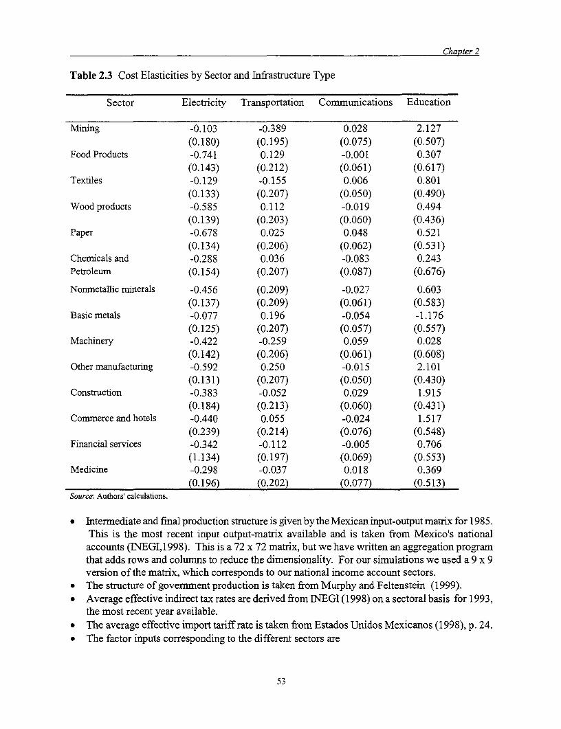
Chapter 2
Table 2.3 Cost Elasticities by Sector and Infrastructure Type
Sector Electricity Transportation Communications Education
Mining -0.103 -0.389 0.028 2.127(0.180) (0.195) (0.075) (0.507)
Food Products -0.741 0.129 -0.001 0.307(0.143) (0.212) (0.061) (0.617)
Textiles -0.129 -0.155 0.006 0.801(0.133) (0.207) (0.050) (0.490)
Wood products -0.585 0.112 -0.019 0.494(0.139) (0.203) (0.060) (0.436)
Paper -0.678 0.025 0.048 0.521(0.134) (0.206) (0.062) (0.531)
Chemicals and -0.288 0.036 -0.083 0.243Petroleum (0.154) (0.207) (0.087) (0.676)
Nonmetallic rminerals -0.456 (0.209) -0.027 0.603(0.137) (0.209) (0.061) (0.583)
Basic metals -0.077 0.196 -0.054 -1.176(0.125) (0.207) (0.057) (0.557)
Machinery -0.422 -0.259 0.059 0.028(0.142) (0.206) (0.061) (0.608)
Othermanufacturing -0.592 0.250 -0.015 2.101(0.131) (0.207) (0.050) (0.430)
Construction -0.383 -0.052 0.029 1.915(0.184) (0.213) (0.060) (0.431)
Comnmerce and hotels -0.440 0.055 -0.024 1.517(0.239) (0.214) (0.076) (0.548)
Financial services -0.342 -0.112 -0.005 0.706(1.134) (0.197) (0.069) (0.553)
Medicine -0.298 -0.037 0.018 0.369(0.196) (0.202) (0.077) (0.513)
Source: Authors' calculations.
* Intermediate and final production structure is given by the Mexican input-output matrix for 1985.This is the most recent input output-matrix available and is taken from Mexico's nationalaccounts (INEGI,1998). This is a 72 x 72 matrix, but we have written an aggregation programthat adds rows and columns to reduce the dimensionality. For our simulations we used a 9 x 9version of the matrix, which corresponds to our national income account sectors.
* The structure of government production is taken from Murphy and Feltenstein (1999).* Average effective indirect tax rates are derived from INEGI (1998) on a sectoral basis for 1993,
the most recent year available.* The average effective import tariff rate is taken from Estados Unidos Mexicanos (1998), p. 24.* The factor inputs corresponding to the different sectors are
53

Chapter 2
1. Agriculture: land, rural labor
2. Mining and resource extraction: capital 1, urban labor
3. Manufacturing: capital 1, urban labor
4. Construction: capital 2, urban labor
5. Electricity, gas, water: capital 3, urban labor
6. Commerce, restaurants: capital 4, urban labor
7. Transport: capital 4, urban labor
8. Financial services: capital 5, urban labor
9. Commerce: capital 5, urban labor
* We derive shares of different financial instruments in financing the budget deficit of the publicsector from the same computer package. This gives us financing from domestic borrowing,money creation, and foreign borrowing.
* Foreign borrowing by the government, in US dollars and foreign borrowing by the private sectorare taken from Estados Unidos Mexicanos, EUM, (1998) pp. 122 and 108 for 1997.
* Initial allocations of factors, capital, land and labor are taken from CD Cuentas Nacionales for1993. We define a unit of the factor as the amount that earned 1 mxp in the base year.
* Initial allocations of money, Ml, for 1997 and while bonds, derived as the 1997 internal debt ofthe federal government are taken from EUM, (1998), pp.9 2 . Allocations of foreign U.S. dollarassets are given by central bank reserves for 1997. EUM, (1998), pp.8 2 .
* Utility weights, assumed to be the same for both urban and rural consumers, are taken asexpenditure shares. These in turn are derived from the aggregation of the 1985 input-outputmatrix.
54

Chapter 2
Simulations
The Benchmark Case
2.41 We now run a six period simulation, that should serve as our benchmark exercise. The goal isto demonstrate that the parameterized model generates results that are consistent with historicaloutcomes in Mexico. Accordingly, we use 1994 as the base year and run a simulation for thefollowing six years. We have historical data for 1995-97, so we can compare actual and simulatedoutcomes for those years. We assume that exogenous policy parameters, such as tax rates, takes ontheir historical values. Table 2.4 shows the resulting macroeconomic outcomes.
Table 2.4 A Benchmark Simulation, 1995-2000 (numbers in parenthesis are historical values).1995 1996 1997 1998 1999 2000
Nominal CTDP 100.0 (100.0) 134.9 (136.3) 186.6 (173.3) 249.5 302.6 419.6Price level 100.0 (100.0) 129.0 (129.6) 170.1 (153.9) 230.8 269.5 378.6Inflation ratea na 29.0 (29.6) 31.9 (18.8) 35.7 16.8 40.5Real GDP 100.0 (100.0) 104.6 (105.2) 107.9 (112.6) 108.0 112.3 110.8Interest rateb 5.0 (37.8) 14.3 (20.7) 16.1 (12.4) 29.0 21.6 35.3Trade Balance (% GDP) 1.4 (2.7) 4.1 (2.1) 2.6 (0.0) 3.8 2.1 2.9Exchange rateb 100.0 (100.0) 122.5 (118.4) 198.5 (123.3) 238.2 325.2 397.4
a. The GE model generates a price level in each year. It is normalized to 1 00 in the first year, hence 1995. Thus you can calculate the rate ofinflation in each year after the first year as P(t)/P(t-l)-l. There is no price level for 1994, since that is before the modelbegins, hence, you cannot calculate a simulated rate of inflation for 1995. Of course there is a real world rate of inflationavailable for 1995, but it is pointless to compare it with a non-existent model number for that year.b. Exchange rates are normalized to the 1995 rate. We use period averages for the historical exchange rates.Source: Author's calculations except as indicated.
2.42 We can make certain observations. Our model does reasonably well in replicating growthrates in both nominal and real income for the three years for which we can make comparisons. RealGDP stagnates after year five, primarily because of the rising interest rate. The simulated tradebalance shows a small surplus throughout the period of the exercise, which is consistent with theassumed floating exchange regime, as well as with historical reality. At the same time, our exchangerate regime generates a small, but steady, real devaluation.
A Shock to Confidence in the Banking System
2.43 It now seems reasonable to use our model to generate counterfactual simulations. As a firstexample let us consider an internal shock. In particular, let us suppose that the economy suffers anunexpected exogenous shock that causes increased anxiety among consumers regarding their bankdeposits. One could argue that such an event is currently happening in Mexico in reaction to thecrisis in Brazil. That is, a financial crisis in one country causes a loss of confidence in the homecountry, even though no reason for such a loss of confidence is apparent. This anxiety is reflected bya fall in the interest elasticity, as demand for money becomes less interest-sensitive because thepublic is suspicious of the banking system.
55

Chapter 2
2.44 To give some numerical value to our example, we will suppose that the elasticity of moneydemand declines from its estimatedvalue of 0.269 to 0.219.1O This reductioninthe elasticitymeansthat, in response to an interest rate increase, consumers are less likely to shift their portfolio structurefrom money into bank deposits. Such a reduction might be caused by, for example, a loss ofconfidence in the banking system's stability. Of course, the actual numerical value of the reductionwe impose is arbitrary. All other exogenous parameter values are assumed to stay the same, and nopolicy response to the shock occurs. The results are given in Table 2.5
Table 2.5 Reduction in the Interest Elasticity of Money Demand, 1995-2000
1995 1996 1997 1998 1999 2000
Nominal GDP 90.6 118.7 158.5 209.9 252.0 343.7Price level 90.8 114.0 147.2 195.4 225.4 311.8Inflation rate na 25.6 29.1 32.7 15.4 38.3Real GDP 99.8 104.2 107.7 107.4 111.8 110.2Interest rate 4.5 14.2 16.3 30.9 23.1 38.3Trade balance (% GDP) 1.4 4.2 3.2 4.1 2.8 3.4Exchange rate 91.9 108.8 174.6 203.3 277.2 332.5Source: Author's calculations.
2.45 The relatively small decrease in the interest elasticity has had measurable effects on theequilibrium outcomes. As might be expected, the price level has declined and the real interest ratehas increased. As a result, real GDP has declined by about 0.6 percentage points, on average, as realinvestment has declined. The trade balance has remained relatively unchanged, given the model'sfloating exchange rate.
2.46 Now suppose that infrastructure had been growing at a faster rate from the time the shock tookhold. In particular, consider a 60 percent increase in real spending on infrastructure in each year ofthe simulation, divided between the four types of infrastructure in proportion to their shares in thetotal stock of infrastructure. Thus the higher rates of infrastructure growth are already in place whenthe interest elasticity shock occurs. Table 2.6 presents the results of this exercise.
10. The numerical value of this reduction is, of course, arbitrary and is used solely to give a sense of the sort ofmagnitudes that we mnight consider.
56

Chapter 2
Table 2.6 Interest Elasticity Decline Combined with an Infrastructure Increase 1995-2000.
1995 1996 1997 1998 1999 2000
Nominal GDP 97.5 128.6 175.2 235.2 285.6 396.2Price level 96.2 121.5 157.2 211.8 242.5 341.2Inflation rate na 26.3 29.4 34.7 14.5 40.7Real GDP 101.4 105.8 111.4 111.1 117.8 116.1Interest rate 5.4 15.2 18.3 32.2 25.2 39.2Trade balance (% of GDP) 1.4 4.1 2.7 3.8 2.3 3.0Exchange rate 96.3 115.6 187.9 223.1 304.4 383.0
Source: Author's calculations.
2.47 The increased expenditure on infrastructure has raised the price level. Such an outcomemight be expected because of the rise in the budget deficit. At the same time, however, the realinterest rate has fallen, primarily because of the increased productivity of capital. This, in turn, is aresult of the higher provision of public infrastructure from the beginning of the simulation. As aresult, real GDP has risen compared with table 2.5, and is now actually higher than in table 2.4,where no elasticity shock occurred. All other macro economic aggregates remain approximatelyunchanged. Thus providing higher rates of infrastructure spending before a shock may, indeed,negate the effects of the shock.
2.48 As noted in the introduction, Aschauer's (1997) partial equilibrium approach indicates that a63 percent real increase in government capital expenditures would lead to about a 0.6 averageincrease in the rate of real GDP growth. A comparison of tables 2.4 and 2.5 shows that a 60 percentreal increase in the corresponding capital expenditure causes the overall growth rate of real GDP torise by 0.7 percent, consistant with Aschauer's results.
Trade Shock
2.49 Let us now consider another type of shock, a stagnation in world income. In particular, realworld income will remain constant for the entire six years of the simulation. This will have a directimpact on Mexico's economy, because real world income affects aggregate demand for export'sequation. Indeed, the estimated elasticity of export demand with respect to world income is 2.33,and in the benchmark simulation world income was assumed to increase. All other parameters willremain the same as in the benchmark case. Table 2.7 gives the results of this exercise.
57

Chapter 2
Table 2.7 Trade Shock: Real World Income Stagnates, 1995-2000
1995 1996 1997 1998 1999 2000
Nominal CUTP 99.2 133.8 183.9 244.6 303.2 40W.9Price level 99.1 128.5 170.4 227.9 270.2 371.5Inflation rate na 29.6 32.6 33.8 18.6 37.5Real GDP 100.0 104.1 108.0 107.3 112.2 110.1Interest rate 4.7 13.8 15.1 28.1 20.4 33.3Trade balance (%GDP) 1.6 3.7 3.5 3.1 3.3 1.8Exchange rate 100.0 141.1 205.8 272.0 340.6 447.4
Source: Author's calculation
2.50 A comparison ofthis case with the benchmark (table 2.4) shows that real GDP is consistentlyabout 0.5 percent lower, the nominal exchange rate depreciates more rapidly, and the Mexicancurrency undergoes real depreciation. The directions and magnitudes of these changes seemplausible. Let us now suppose that the rate of spending on infrastructure was 60 percent higher, inreal terms, than in the benchmark case, and that this was in place before the shock occurred. Table2.8 gives the outcome of this exercise.
Table 2.8 Trade Shock Combined with an Infrastructure Increase, 1995-2000
1995 1996 1997 1998 1999 2000
Nominal GDP 107.6 144.4 203.7 274.4 345.0 469.4Price level 105.7 136.7 182.5 247.5 291.7 405.8Inflation rate na 29.4 33.5 35.6 17.9 39.1Real GDP 101.8 105.6 111.6 110.8 118.3 115.7Interest rate 5.8 14.6 16.9 29.2 21.4 34.0Trade balance (% of GDP) 2.1 3.5 3.1 2.7 2.7 1.4Exchange rate 107.2 149.7 221.3 269.8 373.4 496.7Source: Author's calculations.
2.51 As in the case ofthe internal shock and infrastructure increase, the higherrate of infrastructurespending has brought about a significant increase in real GDP compared with table 2.7. Indeed, theincreased provision of infrastructure has lowered the real interest rate prior to the imposition of theshock, even in comparison with the benchmark case. The increased budget deficit has brought abouta slightly reduced trade surplus in most years, while the domestic price level has risen and theexchange rate has depreciated, compared with table 2.7. Thus once again the results indicate thathaving a higher rate of infrastructure spending in place at the time of a shock tends to alleviate thereal effects of the shock.
2.52 One might ask whether our results stem from the importance of infrastructure in resistingshocks. Could they, on the other hand, be simply the outcome of a public sector spending increase;that is, an increase in aggregate demand? We have therefore carried out a pair of simulations in
58

Chapter 2
which all private cost elasticities with respect to all types of infrastructure are assumed to be 0. Thusinfrastructure is completely ineffective and increases in stocks will not lead to any private sector costefficiencies. We report two simulations. The first is the outcome of the trade shock, assuming 0values for all elasticities. The second, also assuming 0 elasticities, imposes the same 60 percent realincrease in infrastructure spending as in the previous examples. We will only report the real GDPoutcomes, which are given in Table 2.9.
Table 2.9: Infrastructure Elasticities = 0
1995 1996 1997 1998 1999 2000
Shock 97.7 101.7 104.7 104.2 107.8 105.9Shock plus infrastructure 97.9 101.8 104.8 104.3 107.8 105.8
increase
Note: The numbers in the table are real GDP.
We observe that increasing real public expenditure on worthless infrastructure has no effectupon real GDP in the long run, although there is a slight improvement in the initial year. Thus aKeynesian shift in the IS curve leads to no increase in real income, and hence no insulation againstthe shock, unless the expenditure is on useful infrastructure.
59
Chapter 2
Conclusion
2.53 We constructed a dynamic general equilibrium model to analyze issues of stability in theMexican economy and focused on whether an increase in the provision of infrastructure can reducethe impact of exogenous shocks on the real economy. That is, would the impact of a shock be less ifhigher levels of infrastructure spending were in place at the time of the shock?
2.54 Our model incorporates four types of infrastructure in the production process. These areelectricity, telecommunications, transportation, and education. As part of another study (Murphy andFeltenstein 1999), we have estimated their impact on sectoral production functions. In general,increased provision of infrastructure, either by the public or private sector, tends to be cost reducing.We have then incorporated the estimated infrastructure elasticities in the fully parametarized generalequilibrium model.
2.55 Using avarietyofMexican data sources, we calibrated themodel to the years 1995-97 aspartof a six-year simulation for the years 1995-2000. The model generates reasonably accurateapproximations of the macroeconomic outcomes of the actual Mexican economy, therebyjustifyingits use for counterfactual simulations. We then generate a shock to the interest elasticity of moneydemand, causing the absolute value of the elasticity to decline. Such a shock might be caused by asudden loss of confidence in the banking system, and tends to increase holdings of money and reducebank deposits. Over time, this shock brings about an increase in the real interest rate, a deflation,and a reduction in real GDP amounting to about 0.5 percentage points, on average, over the six yearsof the simulations.
2.56 We then suppose that prior to the shock, infrastructure spendingwas 60 percent higher, inrealterms, on each of the four types of infrastructure. The increased provision of infrastructure reducesthe private sector's costs, and as a result, real GDP rises to a somewhat higher level than in the initial,pre shock simulation. We thus conclude that it is, indeed, possible for higher levels of infrastructurestocks to insulate the Mexican economy from certain types of shocks.
2.57 The final set of simulations involves the imposition of an external shock: stagnation of theworld's real income for the six years of the simulation. This lowers the demand for Mexicanexports, and accordingly, the rate of growth of real Mexican income. We then suppose thatexpenditure on all types of infrastructure was uniformly 60 percent higher before the shock occurredand throughout the period of the simulation. Again, this reverses the decline in real Mexican incomeand largely neutralizes the effects of the shock.
2.58 Thus, the positive implications of increased infrastructure provision seem to outweigh thenegative impact on the budget deficit. Enhanced infrastructure, prior to shocks, seems to offer auseful way to avoid the ex post remedies that have been tried so often, and frequently with littlesuccess.
60
Chapter 2
References
Alberro, J. 1989a. "In Search of a Stable Demand for Money in Mexico During the 1969-1987Period," unpublished.
. 1989b. "Capital Outflows in Mexico During the 1970-1987 Period," unpublished.
Aschauer, David. 1997. '?ublic Infrastructure, Capital, and Economic Growth: Some ResultsPertaining to the Mexican Economy" unpublished discussion paper.
Ball, S. and A. Feltenstein. 1997. "Basic Macroeconomic Options for Bangladesh: A NumericalAnalysis" forthcoming, Journal of Asian Economics.
Banco de Mexico. 1998. La Encuesta de Acervos, Depreciacion y Formacion de Capital del Bancode Mexico, Computer disks.
Estados Unidos Mexicanos. 1998. Cuarto Informe de Gobierno, Anexo, Poder Ejecutivo Federal:Presiencia de la Repuiblica, Mexico.
1NEGI. 1998. Cuentas Nacionales de Mexico, CD-ROM.
Feltenstein, A. 1986. "An Intertemporal General Equilibrium Analysis of Financial Crowding Out: APolicy Model and an Application to Australia," Journal of Public Economics, (November),1986, pp. 79-104.
Feltenstein, A. 1992. "Oil Prices and Rural Migration: The Dutch Disease Goes South,"Journal ofInternational Money and Finance, n. 11, pp. 273-291.
Feltenstein, A., and J. Ha. 1995. "The Role of Infrastructure in Mexican Economic Reform," WorldBank Economic Review, v. 9, n.2, pp. 287-304.
1998. "An Analysis of the Optimal Provision of Public Infrastructure: AComputational Model Using Mexican Data," forthcomning, Journal ofDevelopment Economics.
Feltenstein, A., and S. Morris. 1990. "Fiscal Stabilization and Exchange Rate Instability: ATheoretical Approach and Some Policy Conclusions using Mexican Data," Journal of PublicEconomics, (August), 42, pp. 329-356.
Feltenstein, A., and A. Shah. 1995. "General Equilibrium Effects of Investment Incentives inMexico," Journal of Development Economics, 46, pp. 253-269.
International Monetary Fund. Mexico - Recent Economic Developments (various issues),.
Jarque, Carlos. 1988. "An Empirical Study of the Determinants of Production in Mexico"
61
Chapter 2
unpublished manuscript.
Jung, W.S. 1988. "Asset Demands in Mexico," unpublished University of Kansas discussion paper.
Murphy, Russell and Andrew Feltenstein. 1999. "Private Costs and Public Infrastructure: TheMexican Case", unpublished, Virginia Tech.
Paquete de Finanzas Publicas y Deuda Publica (Base de Datos). 1998. 3 disk computer package,provided by the Ministry of Finance of Mexico, that provides disaggregated fiscal time seriesdata.
Shoven, J.B., and J. Whalley. 1984. "Applied General Equilibrium Models of Taxation andInternational Trade," Journal ofEconomnic Literature, vol.22, (September), pp. 1007-105 1.
World Bank. 1998. Mexico: Enhancing Factor Productivity Growth, Country EconomicMemorandum, August.
Zedillo, Emesto. 1986. "Capital Flight: Some Observations on the Mexican Case," Paper presentedat the Conference on Capital Flight and Third World Debt. Institute for InternationalEconomics, Washington, D.C.
Appendix
Investment
Let us adopt the following notation:
ki = investment tax credit in period i (percent)di = depreciation allowance in period i (percent)tki profit tax rate (percent)CHi = the cost of producing the quantity Hi of capital in period iri = the interest rate in period iPKi the return to capital in period iPMi the price of money in period i
Suppose that the rental price of capital in period i +l is PK(+,) . If CHi is the cost of
producing the quantity of capital, Hi, then future debt obligations must equal the return on newcapital. Hence
62

Chapter 2
CHIO - k, - d,) = (l- tK 2 )PK 2 Hl (Al)
where r, the interest rate in period i, given by
ri = 1/PBi (A2)
where PBi is the price of a bond in period i.
Consumption
2.59 Here, and in what follows, x denotes a demand variable and y denotes a supply variable.To avoid unreadable subscripts, 1 will refer to period i and 2 will refer to period i + 1. Theconsumer's maximization problem is thus
Max U(x), x = (xl,xLUl,xLrl,X2,XLu 2 1XLT2 ) (A3)
Such that
(I +ti)PiXi + PLriXLri + PMiXmi +PBiXBi +eiPBflxBF= Ci (A4)PKIKO + PAIAO + PLUILUI + PL,IL,I + PMIMo + roBo + PBI Bo + e,PBFIBFO + TR, = N1
PK2 (1 -)KO + PLu2Lu2 + PLr2Lr2 + PM2XM B + r1XB1 + PB2XBI + e2PBF2XBFI + TR2 N2
C, = N,
logP,ixmi =a +blog(1 +tj)8xj--c1ogrj; c=c(DEFIASSET) (A5)
log PBi XBi-log eiPBFi xBFi=atZ+ p log rj-log-e+IrFi )(A6)
PB2XB2 =S(l+t2 )P2 X2 (A7)
63
Chapter 2
where
Pi= price vector of consumption goods in period ixi= vector of consumption in period i
C =j value of aggregate consumption in period i (including purchases of financial assets)Ni = aggregate income in period i (including potential income from the sale of real and
financial assets)ti = vector of sales tax rates in period i
PL,u =price of urban labor in period iL,i = allocation of total labor to urban labor in period iXYL,,i= demand for urban leisure in period iPLri= price of rural labor in period iL,i= allocation of total labor to rural labor in period i
PKi= price of capital in period iKo = initial holding of capitalPAi = price of land in period iAo= initial holding of land6 rate of depreciation of capital
PMi price of money in period i (money in period 1 is the numeraire, and hence has a priceof 1; a decline in the relative price of money from one period to the next representsinflation)
xmi = holdings of money in period iPBi = discount price of a certificate of deposit in period i
ri= domestic interest rate in period ixBi = quantity of bank deposits, that is, certificates of deposit in period iei = the exchange rate in terms of units of domestic currency per unit of foreign currency
in period iXBFI =quantity of foreign currency held in period iTRi = transfer payments from the government in period i
a, b, a, B estimated constants
DEF = the total value of non-perforning assets in the banking systemASSET = total assets of the banking system
C = a functional form that depends negatively upon the ratio of non performing assets tototal assets in the banking system
2.60 The left-hand side of equation (A4) represents the value of consumption of goods andleisure, as well as of financial assets. The next two equations contain the value of the consumer'sholdings of capital and labor, as well as the principal and interest that the consumer receives from thedomestic and foreign financial assets that he held at the end of the previous period. The equation C1= Ni then imposes a budget constraint in each period. Equation (A5) is a standard money demandequation in which the demand for cash balances depends upon the domestic interest rate and thevalue of intended consumption. There is, however, one modification. The interest elasticity, c,
64
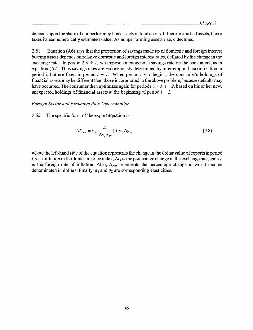
Chapter 2
depends upon the share of nonperforming bank assets in total assets. If there are no bad assets, then ctakes its econometrically estimated value. As nonperforming assets rise, c declines.
2.61 Equation (A6) says that the proportion of savings made up of domestic and foreign interestbearing assets depends on relative domestic and foreign interest rates, deflated by the change in theexchange rate. In period 2 (i + 1) we impose an exogenous savings rate on the consumers, as inequation (A7). Thus savings rates are endogenously determined by intertemporal maximization inperiod i, but are fixed in period i + 1. When period i + 1 begins, the consumer's holdings offinancial assets may be different than those incorporated in the above problem, because defaults mayhave occurred. The consumer then optimizes again for periods i + 1, i + 2, based on his or her new,unexpected holdings of financial assets at the beginning of period i + 2.
Foreign Sector and Exchange Rate Determination
2.62 The specific form of the export equation is:
AXno =oa[ er ]±+2 Ay\Ywi (A8)/Aei7rFi
where the left-hand side of the equation represents the change in the dollar value of exports in periodi, 7ri is inflation in the domestic price index, Aei is the percentage change in the exchange rate, and 7rFi
is the foreign rate of inflation. Also, AyWi represents the percentage change in world incomedenominated in dollars. Finally, a, and a2 are corresponding elasticities.
65

INFRASTRUCTURE, PRIVATE COSTS, AND PAYOFFS FROM ADDITIONSTO INFRASTRUCTURE
3.1 This chapter provides estimates of the potential (partial equilibrium) payoffs fromincreased investment in public infrastructure and calculates (in a static context) the optimalinfrastructure stocks implied by the elasticity estimates. The chapter also considers the role thatpublic infrastructure plays in improving the efficiency of the private sector. In particular, itfocuses on the short-run, static gains that accrue to private firms because of governmentinvestments in electric, transportation, and communications infrastructure. We also consider thepotential role of education in reducing private sector costs, but ultimately conclude that theeducation estimates are not particularly informative, primarily because of the nature of the dataused.
3.2 The role public spending plays in enhancing economic productivity has long been aconcern for policymakers. In recent decades, public expenditure has primarily been evaluated interms of two roles: enhancing macroeconomic stability and mitigating market failure. An equallyimportant role concerns the ability of public investments in infrastructure capital to reduce thecosts of private firms. Particularly for developing economies, this role may be critical because itmay allow the private sector to become more resilient to external shocks. A major concernrelated to the recent fiscal adjustment in Mexico is that it was carried out partly by depletingpublic infrastructure stocks. This depletion could significantly retard future growth by imposingan additional drag on private sector costs and output.
3.3 This chapter shows that public infrastructure in Mexico has generally small, butsignificant, negative effects on private sector costs. The base case estimates of the elasticity ofprivate sector costs with respect to infrastructure suggest a mean value of -0.106 across 14sectors of the economy (with a range of -0.563 to 0.355). In general, electric infrastructureappears to have the most beneficial effects on private sector costs (mean base case elasticity of-0.171), and transportation infrastructure has the next most beneficial effects (mean base caseelasticity of -0.165). Communications infrastructure appears to have little effect on private sectorcosts (the mean base case elasticity is 0.019), but all the base case t-ratios are less than 2.0,indicating that the estimates are not statistically significant.' Education infrastructure elasticity
1. Only 2 of the 14 are larger than 1.0.

Chapter 3
estimates are mixed and difficult to interpret, and most are also statistically insignificant.2
3.4 The communications and education elasticity estimates are surprising. Why are theseestimates so different from our priors? Why are the education estimates at such variance withdifferent, but potentially related figures such as estimates of the social returns to human capitalof roughly 10 to 20 percent. (See Psacharopoulos 1994, who reports social returns of 10 to 14percent for Mexico in the mid 1980s and 12 to 18 percent for Latin America as a whole). Foreducation, these results are likely the result of the combination of two facets of the analysisrather than indications of the true productive (or unproductive) nature of investments ineducation. The analysis is based on aggregate data for several sectors of the Mexican economyduring the period 1960-93. We measure technical progress by time. Unfortunately (for theanalysis), Mexican investment in education has been relatively steady in recent decades whichmeans that there is little opportunity econometrically to separate the effects of time (technicalprogress) and education.
3.5 The most sensible interpretation of the education elasticities is that our aggregate data donot allow us to infer much about the productive spillovers of public investment into humancapital. An alternative approach, based on observations of individual workers and firms, wouldbe more appropriate for understanding the role of education, because we would be able toobserve more variation of educational levels and private sector costs across firms. Investigatorstypically use a micro data approach to estimate social returns to human capital investments.
3.6 The small, positive, and insignificant estimates of the elasticity of private sector costswith respect to investments in communications infrastructure are similar to the estimates of theproductivity-enhancing effects of high technology investments in the United States (Stiroh1998). Some studies (Canning 1998) have found that communications infrastructure (measuredin terms of main lines per capita) is productive, but in general the productivity-enhancing effectsof high technology are not immediately apparent in aggregate data. Several explanations couldaccount for this odd result. One possibility is that reduced technology costs induce firms to factorsubstitute, but do not lead to significantly lower costs. In the United States there are indications,even from the micro data, that while technology use and lower costs are associated, firms that areproductive in other ways (good performers) tend to be the ones that use technology, rather thantechnology use leading to lower costs (McGuckin, Streitweiser, and Doms 1996). This is similarto Hulten's (1996) argument that, in the words of the paper's title, how well you use it may bemore important than how much you have.
3.7 Using the electricity, transportation, and communications estimates, rough calculationsbased on these elasticities suggest that a 1 percent increase in public infrastructure stocks wouldcost approximately mxp 6.6 billion and provide annual benefits across 14 sectors of the economyof mxp 12.4 billion (both in terms of real 1980 pesos). These are static, partial equilibriumestimates, but they suggest that at least in the short run, additional investment in publicinfrastructure stocks could be welfare improving. Given sensible depreciation rates, the presentvalue of these benefits over future years might be roughly nine times the single year grossbenefits. If the base case elasticity estimates are correct, static calculations of the optimal size of
2. Only 4 of the 14 have t-ratios larger han 2.0 in absolute value.
67

Chapter 3
infrastructure stocks suggest that electric and transportation stocks should have been 2.5 and 4times as large as they actually were in 1993.
3.8 However, one of the striking features of the elasticity estimates is that they are generallysmall (the effects of public infrastructure on private sector costs do not appear to be large) andsomewhat noisy (the estimated effects vary, sometimes significantly, across sectors). Thissuggests that a degree of caution is warranted in interpreting the estimates. If large potentialbenefits were associated with public infrastructure, the effects should have been clearer in thedata. The estimates do suggest a role for public sector infrastructure capital in reducing privatesector costs, but a modest role.
3.9 The results presented in this chapter represent improvements over the existing literaturein several respects as follows:
* We consider the role of education as a potential type of public infrastructure.
* We explicitly evaluate the role of different assumptions about cost function characteristicssuch as returns to scale.
- We calculate the precision of estimates of the elasticity of private sector costs with respect topublic infrastructure, rather than just point estimates.
- We consider the potential effects on the estimates of cross-sector heteroskedasticity andcross-time autoregression.
* We calculate the optimal infrastructure levels implied by the elasticity estimates.
3.10 The next section of the chapter briefly discusses the relevant policy environment. It thenintroduces the basic model and the related conceptual issues, briefly considers the data used foranalysis, and discusses empirical implementation. This is followed by the empirical results and aconcluding section. Several annexes discuss details of the production cost estimation model,econometric specification issues, construction of the dataset, and detailed regression results.
Background
3.11 Our dataset is confined to the period 1960-93, so the overview focuses on this period aswell, recognizing that unfortunately we neglect the most recent years. This is necessitated by ourneed to construct a dataset from several sources, not all of which are currently available for thesame periods in the form required (see appendix C).
3.12 Gross domestic product grew strongly during 1960-93. Average growth in real termswas 0.049 per year during this time, and only 1982, 1983, and 1986 saw real declines inaggregate output (INEGI 1997). Furthermore, this growth was experienced across the economy(table 3.1). If anything, infrastructure growth was even more impressive; during this period.Electricity and communications stocks (total net capital stock, in real 1980 pesos, see appendix
68

Chapter 3
C) grew by 0.137 and 0.255 annually (compound annual rates, see table 3.2).
Table 3.1: Compound Annual Growth Rates 1960-93 (real 1980 pesos)
Major Sector GDPSector Sector Growth
Mining 2 0.048Food and tobacco 3 1 0.043Textiles 3 2 0.029Wood products 3 3 0.034Paper 3 4 0.051Chemicals 3 5 0.070Nonmetallic minerals 3 6 0.055Basic metals 3 7 0.052Machinery 3 8 0.068Other manufacturing 3 9 0.028Construction 4 0.048Conmmerce, hotels 6 0.051Financial services 8 0.047Medicine 9 0.048
Table 3.2: Ihfrastructure Compound annual Growth rates, 1960-93 and 1983-93 (real 1980pesos)
Sector 1960-1993 1983-1993Electricity 0.137 -0.003Transport 0.063 0.029
Communic 0.255 0.075ationsEducation 0.021 0.021
3.13 Physical infrastructure stocks have increased at rates comparable to, or perhaps a littlehigher than, rates in several other Latin American countries (Table 3.3 2). The table presents
2 Based on data from Canning (1998), which also include measures of telephones, unpaved roads, and rail lines. Themnain lines data (communications) and paved roads data (transportation) are of most interest here since they presentthe best opportunities for spillover effects which would appear in the national accounts data.
69

Chapter 3
averages of annual growth rates for several periods; the first column is for the whole period; thelast column is for the most recent ten years. Growth has been, on average, somewhat lower inMexico in recent years.
Table 3.3: Physical infrastructure (average annual growth rates)
1950-1995 1950-1970 1970-1990 1980-1995 1985-1995
Electric
Mexico 0.120 0.176 0.071 0.068 0.065
Argentina 0.057 0.072 0.049 0.034 0.021
Brazil 0.081 0.096 0.082 0.038 0.030
Chile 0.048 0.053 0.036 0.033 0.060
Colombia 0.084 0.119 0.064 0.056 0.070
Venezuela 0.098 0.121 0.096 0.057 0.053
Telephone main lines
Mexico 0.087 0.074 0.096 0.082 0.091
Argentina 0.053 0.035 0.046 0.077 0.076
Brazil 0.093 NA 0.099 0.068 0.064
Chile 0.087 0.081 0.068 0.120 0.138
Colombia 0.079 0.081 0.073 0.090 0.086
Venezuela 0.092 0.094 0.088 0.079 0.074
Paved roads
Mexico 0.020 0.058 -0.045 0.019 0.019
Argentina 0.045 0.086 0.031 0.014 0.012
Brazil 0.123 0.212 0.067 0.051 0.039
Chile 0.041 0.091 0.021 0.018 0.038
Colombia 0.052 0.077 0.038 0.021 0.024
Venezuela 0.042 0.086 0.018 0.027 0.033
70

Chapter 3
3.14 Our financial measures are more convenient for analysis, and are reasonableapproximations to the measures of physical infrastructure reported by Canning (1998). Figure 1shows changes in (log3 ) electric, transport, and communications infrastructures over past severaldecades. The physical and financial measures of electric infrastructure, with the exception of theearly 1960s, moved pretty much in tandem over the past few decades. The transportationmeasures also move similarly, although there is a substantial jump in (financial) value in the late1970s. Prior to, and after, this two year jump, the measures move in similar fashions. The valueof communications infrastructure also makes a substantial jump in the late 1970s; an increasewhich we do not see in the telephone main lines data. This, like the jump in transportinfrastructure, may be due to quality changes which the physical measures do not capture.
Figure 3.1 Changes in electric, transport, and communications infrastructure (log 3 )
1000000 -1000000 l
,.. -----------
100000 - --
.o ~~~~~~~~~~~~~100000 .'
10000~~~~~~~~~~~~~~100
1000 100001960 1965 1970 1975 1980 1905 1990 1995 1960 1965 1970 1975 1980 1985 1990 1995
- Electric generating capacity - - - - Electic inc atucture PavedToads ------- TranspoTtation infrastnrctire
100000 - _ _
10000
1OO'. _. ___
loo --
10I
1960 1965 1970 1975 1980 1985 1990 1995
- Tel Main limes ------ Comm. infrastructure
3.15 Table 3.4 shows correlations between the physical and financial measures; the
3 The data are reported in logs to facilitate comparisons of growth rates, which are more relevant in this context thanmagnitudes.
71

Chapter 3
correlations between the logs of financial and physical measures are all over 90 percent; thecorrelations between growth rates are lower, but with the exception of the transport measures,even the growth rates of financial and physical measures are positively correlated.
Table 3.4 Correlations: physical and financial infrastructure measures
In,frastructure ln(Levels) Growth rates
Electric
(generating capacity) 0.9152 0.4766
Transport
(paved roads) 0.9855 0.0638
Comimunications
(main lines) 0.9774 0.3594
3.16 Clearly, however, investment has slowed significantly in recent years. This recentdecline is even more noticeable in the post-sample period 1994-98. It prompts the concern thatwhile necessary for short-term, pressing budgetary reasons, these reductions in publicinfrastructure will ultimately prove to increase costs in the private sector, perhaps even to theextent of raising private sector costs by more than the short-term public sector savings.
The Model
3.17 The model of private sector costs in the Mexican economy is based on a standardtranslog cost model: an approximation of a general private sector cost function from a first-orderTaylor series expansion in logs of a transcendental function (see Berndt 1991, chapter 9 and thereferences cited therein; Takayama 1990). In the following presentation, the data dimensions ofinterest (and their associated indices) are private inputs (indexed by i (- {L,K}) governmentinfrastructure (indexed by m), sectors (indexed byj), and time (indexed by t). For brevity, thetime index is ordinarily suppressed.
3.18 In each sector], the basic specification relates production costs (c) to input prices (w),
72
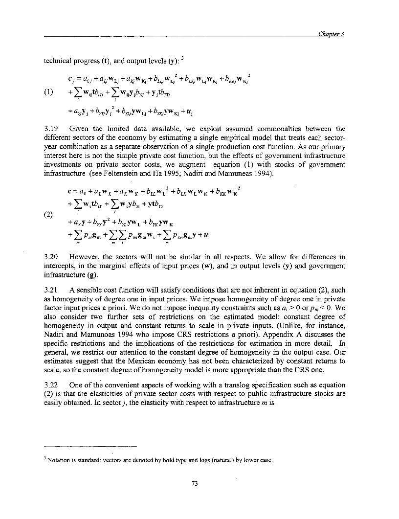
Chapter 3
technical progress (t), and output levels (y): 3
Cj = a,j + aLjwLj + aKjwKj + bljwLj 2 + bjwLJwKj + bKKjWKj
(1) + wijtbiTj + wijyjbyij + yjtbTr
+nay; + byj 2 + byjYW +bywKJ + Uj
3.19 Given the limited data available, we exploit assumed conmmonalties between thedifferent sectors of the economy by estimating a single empirical model that treats each sector-year combination as a separate observation of a single production cost function. As our primaryinterest here is not the simple private cost function, but the effects of government infrastructureinvestments on private sector costs, we augment equation (1) with stocks of governmentinfrastructure (see Feltenstein and Ha 1995; Nadiri and Mamuneas 1994).
+KaLWL +aKW +bLLWL +bLKWLWK +bKWK
+ ±witbiT + ,wiybyi + ytb77(2) i E
+ayy+by 2 +±bYywL +byKYWK
+ Pmg. +Epjimgmwi + pymg.y+um m i m
3.20 However, the sectors will not be similar in all respects. We allow for differences inintercepts, in the marginal effects of input prices (w), and in output levels (y) and governmentinfrastructure (g).
3.21 A sensible cost function will satisfy conditions that are not inherent in equation (2), suchas homogeneity of degree one in input prices. We impose homogeneity of degree one in privatefactor input prices a priori. We do not impose inequality constraints such as ai > 0 orpm < 0. Wealso consider two further sets of restrictions on the estimated model: constant degree ofhomogeneity in output and constant returns to scale in private inputs. (Unlike, for instance,Nadiri and Mamunoas 1994 who impose CRS restrictions a priori). Appendix A discusses thespecific restrictions and the implications of the restrictions for estimation in more detail. Ingeneral, we restrict our attention to the constant degree of homogeneity in the output case. Ourestimates suggest that the Mexican economy has not been characterized by constant returns toscale, so the constant degree of homogeneity model is more appropriate than the CRS one.
3.22 One of the convenient aspects of working with a translog specification such as equation(2) is that the elasticities of private sector costs with respect to public infrastructure stocks areeasily obtained. In sectorj, the elasticity with respect to infrastructure m is
3Notation is standard: vectors are denoted by bold type and logs (natural) by lower case.
73

Chgater 3
(3) elm = Pm + PimWi + PymY
3.23 Because the estimated elasticities are simply linear combinations of estimatedcoefficients, their variances are simple to calculate as well. Let A = [1 WL WK y] and
b=[P. PL. PK. Pym] . Then ejm= Ab and V1(ejim )=AV(b)A'. In the elasticity calculations
below, we construct values for A from the average (over the relevant sample horizon) values ofw and y; we treat those values as constants.
The Data
3.24 We briefly discuss the data used in this analysis here. See appendix A for complete,detailed documentation.
Sources
3.25 All data derive from official Mexican government sources. The two primary sources areINEGI (1997) and Banco de Mexico (1995). For 1980-93, the data were taken from thegovernment sources with little adjustment. For earlier periods (1970-80 and 1960-70), data serieswere often constructed from multiple sources. Appendix C describes these procedures in detail.
3.26 The sectors we use are determined by the Sistema de Cuentas Nacionales de Mexico(SCNM). Our basic delineation of the Mexican economy includes 17 sectors. One, agriculture, isdropped because of a lack of capital stock data. We used two others, electricity (sector 61, majorsector 5) and transport and communications, (Sectors 64 and 65, or major sector 7) are used toconstruct our estimates of public infrastructure. This left us with 14 sectors for analysis (see table3.6 for a list).
The variable definitions are as follows:
pb Gross sectoral output in real 1980 pesospib Sectoral value added in real 1980 pesoslabor Workers employed in the sector (millions)gwage Mean annual sectoral wages in real 1980 pesoslmpts Sectoral payments to labor in real 1980 pesoscap Total sectoral net capital stock in real 1980 pesostbill Treasury bill rate (Mexico)cmpts Sectoral payments to capital in real 1980 pesosielec Electricity infrastructure (total net capital stock of Sector 61 of the SCNM)itran Transport infrastructure (Sector of the SCNM)icomm Communications infrastructure (Sector 65 of the SCNM)primed Index of adult population with at least primary school
74

Chapter 3
Table 3.5 presents the variables of interest and their sample means and standard deviations.
Table 3.5 Primary Data: Means and Standard Deviations (millions of real 1980 pesos)
Variable 1960-93 1960-69 1970-79 1980-93
Pb 333,788 156,940 298,529 485,294(349,484) (131,115) (250,968) (440,396)
Pib 209,708 98,471 186,757 305,555(283,186) (116,221) (221,609) (363,613)
Labor 0.777 0.414 0.735 1.067(1.347) (0.645) (1.160) (1.727)
Gwage 114.0 85.0 134.4 120.2(52.3) (35.5) (47.7) (56.5)
Lpmts 71,277 37,780 74,411 92,964(110,401) (52,010) (103,922) (137,032)
Cap 38,963 17,308 39,159 54,292(34,646) (15,939) (29,598) (39,312)
Tbill 0.150 0.039 0.070 0.288(0.136) (0.012) (0.025) (0.108)
Cpmts 117,082 40,467 104,317 180,925(164,152) (47,853) (134,742) (206,483)
Ielec 195,837 47,624 178,566 314,041(117,121) (26,934) (58,108) (21,461)
Itran 114,124 35,558 90,504 187,115(69,499) (4,729) (30,611) (29,910)
Icomm 30,784 163 10,817 66,917(33,718) (106) (12,535) (19,640)
Primed 0.163 0.134 0.165 0.182(0.024) (0.016) (0.007) (0.014)
Source: Author's calculations.
Sample horizon
3.27 Our dataset covers 1960-93. Because of the significant changes in the Mexican economyduring this time, we estimated models for several subsamples of this period. In particular, weconsider models of the periods 1960-79, 1974-1993, and 1960-93. Our base case was the 1974-93 subsamples because this period should most closely reflect the modem Mexican economy.
Data Limitations
3.28 This analysis is subject to several potential limitations. First, the data include only the
75

Chapter 3
period through 1993 thus to the extent that the experience of the past five years is particularlyinformative about the effects of public sector infrastructure on private sector costs, the analysiswill be deficient. By restricting the base case estimates to 1974-93, we hope that this problemwill be partially mitigated as the estimates are based on relatively recent history.
3.29 , This chapter takes an initial step toward evaluating the role public education has playedas a component of the Mexican economy's infrastructure. Nonetheless, this step is not entirelysatisfying, in part because of data limitations (see appendix C). The private sector cost elasticitiesthat are most compelling are those that ignore education. This is a limitation of the data. Theanalysis does not provide compelling evidence either that education has no cost saving role orthat it has a significant cost saving role. Instead, despite our attempts to date, we are unable toprovide evidence one way or the other.
3.30 The Mexican economy exhibits considerable variation across different geographic areasand within the same industrial sector. This variation is masked in the aggregate data with whichwe work. One can consider this as a form of measurement error. Hence our coefficient estimatesare likely to be biased (in absolute value) toward zero.
Estimation of the Model
Methods
3.31 The translog model allows for convenient simplification of the cost equation (2) into aset of share equations (see appendix A). Each represents the share of total costs for a privatefactor. In our case, with only two factors (labor and capital), we only need to estimate one shareequation because the shares sum to one. We arbitrarily choose to use the labor share equation(given our estimation method, the coefficient estimates should be invariant to this choice).Therefore, let the translog model encompass a cost equation and a labor share equation. Thisallows us to estimate (in a seemingly unrelated regression framework) the two equationssimultaneously and gain efficiency.
Infrastructure
3.32 The data include measures of public infrastructure in four areas: electricity,transportation, communications, and education. In the cases of electricity, transportation, andcommunications, we consider total net capital (the sum of net capital in buildings andconstruction projects, machinery, transportation equipment, and office equipment) as ourmeasure of infrastructure. Typically, these stocks are measured in real 1980 pesos. In the case ofeducation, we use an index representing the proportion of the adult population with at least aprimary school education.
3.33 The education measure is suspect for several reasons. First, while the development andlabor literatures speculates that primary school education is particularly important for economicdevelopment, this claim is by no means certain. For this reason, alternative measures ofeducational infrastructure deserve close attention in the future. Second, even if primary school
76

Chapter 3
education is the appropriate infrastructure benchmark for Mexico, our measure is likely to beprone to measurement error. One form of measurement error arises because the penetration ofprimary school education is likely to vary across different parts of the Mexican economy: bygeographic area, by workers' ages, and by sector of the economy. A second form of measurementerror arises from the lengths to which we had to go to construct our index (see appendix C).Finally, because of the significant and relatively sustained growth in educational attainment inthe Mexican work force during the past 30 years, our measure exhibits little variation that is,growth is concentrated somewhat in the early and later years, but is monotonic (see figure 3.2).More than 85 percent of the variation in the education index can be explained by a time trend;however, our model already captures technical progress by a time trend. For this reason, theeducation measure is unlikely to provide informative estimates.
Figure 3.2 Education infrastructure index
Education Infrastructure Index
0.25
' 0.20
0. 90 0.150 0-u
., '0.10
0 E
0
0. 0.00.
1960 1965 1970 1975 1980 1985 1990 1995
For all these reasons, we consider estimates both with and without the education infrastructurevariable. On the whole, the without education estimates are more plausible.
Estimation limitations
3.34 The formulation of the problem in equation (2) is not entirely satisfactory. There are twoestimation issues related to the role of input prices. The first is that for the economy as a whole,presumably the prices of capital, r, and labor, w, are endogenous. If so, OLS and similarestimators will be inconsistent. Ideally, we would instrument for factor prices, however, in theabsence of good instruments, we argue that factor prices in Mexico are determined in a worldmarket. For our purposes, private factor prices are not endogenous.
3.35 A second objection to the structure above is that instead of government infrastructure
77

Chapter 3
stocks, one would preferably use prices (much as we use private factor prices). If infrastructure isacquired and utilized in the same fashion as other inputs, this objection is appropriate. Here, theuse of stocks may not be problematic. Recall that our interest is in the spillover effects ofpublicly provided infrastructure; we estimate those spillovers through the translog model. Thetranslog specification is appropriate not because our priors (based on, e.g., engineering data)suggest that costs vary as in equation (1), but because equation (1) is a good approximation to anarbitrary cost function. We allow the data to tell us how costs are affected by the inputs. Use ofprivate inputs such as capital and labor, from standard cost theory, are determined by factorprices; therefore r and w are crucial regressors. By extension, this is why one would want toinclude infrastructure usage costs in equation (2). However, in the case of infrastructure,utilization, or congestion, would be more desirable than prices; firms do not demandinfrastructure services, they use the services that are available. Presumably private sector costsvary with utilization, z:
C zGu
or in logs:
c z+g+u
3.36 The problem is an omitted variable one; we estimate c g + u rather than c z + g + u .The effects of utilization on costs will be, in our formulation, attributed to the disturbance termu; if cov(z,g) • 0, the estimates of the effect of government infrastructure, g, on private costs cwill be inconsistent. However, if utilization is uncorrelated with infrastructure levels, theestimates of the cost reducing effects of infrastructure will not be adversely affected by theomission of utilization from the estimated model. A sufficient, but not necessary, condition forthis (omission of utilization not biasing the estimated effects) is that government infrastructure isutilized at the same rate each period. But, a weaker condition, that utilization is not correlatedwith infrastructure levels, is also sufficient. This assumption is more plausible and is the one thatwe make.
3.37 The Mexican economy is apt to exhibit considerable variation across differentgeographic areas and within the same industrial sector. This variation is masked in the aggregatedata with which we work. One can consider this as a form of measurement error; hence, ourcoefficient estimates are likely to be biased (in absolute value) toward zero.
Results
3.38 Our primary interest is in the effects of public infrastructure on private sector costs. Oursummary measures of these effects are the elasticities of private sector costs with respect to thevarious infrastructure measures. The base case consists of estimates based on
* The period 1974-93
* The stocks of electricity, transport, and communications infrastructure (but not education)
* A constant degree of homogeneity in output.
78

Chapter 3
Overview
3.39 Tables 3.6-3.9 present the estimated elasticities and their standard errors for fourdifferent specifications of the basic translog model. The first, which we call our "base case,"includes the three main (measurable) infrastructure stocks: electricity, transport, andcommunications. Recall that we exclude education, not because it is unimportant, but because wecannot econometrically separate the effects of education from the effects of our measure oftechnological progress. The base case estimates are calculated imposing the constraint that costsare homogeneous of degree one in output (doubling output doubles private sector costs).
3.40 The "no restrictions" specification considers how the estimated effects of infrastructurechange if we do not impose as many constraints on the basic translog model. The onlyconstraints imposed on the basic translog specification are those necessary for homogeneity ofdegree one in input prices. The estimates, overall, are not too different from the base caseestimates. The no restrictions estimates of the effects of electric infrastructure are slightly morenegative, while the estimated effects of transport infrastructure are less so. The estimatedcommunications effects are quite similar.
3.41 The constant returns to scale model is similar to the base case, but an additionalconstraint is imposed: the scale of operations does not change marginal costs. Imposing theconstant returns to scale constraint generates larger (more negative) estimated effects of electricinfrastructure, but smaller (more positive) estimated effects of transport and communicationsinfrastructure. A test of rejects the null hypothesis that costs are characterized by CRS.
3.42 The cost elasticity estimates are generally plausible: as table 3.6 shows, the magnitudesare not overly large and most elasticities have appropriate signs (see appendix A for more detailsabout the estimated models). Of the 14 base case elasticity estimates for electricity, 10 arenegative with values of roughly -0.20. The estimated standard errors are in the range of 0.10-0.16. The smaller (in absolute value) elasticity estimates are, by conventional standards,insignificantly different from zero. The larger values (for instance, for sectors 2, 4, and 5),however, do tend to be several times the size of their standard errors. The transportationestimates are fairly similar. Of the 14, 12 are negative and many take on values around -0.15 or-0.35. Again, the standard errors are roughly 0.15.
3.43 The communications elasticities, however, are generally quite small (roughly 0.05), thewrong sign (9 of the 14 are positive), and imprecisely estimated (standard errors of 11 of the 14are larger than their corresponding coefficients).
3.44 The alternative cases generally present a mixed picture. The model with educationgenerates coefficient estimates that are mostly negative (9, 10, 12, and 10 of the 14 sectors foreach of the electricity, transport, communications, and education infrastructures, respectively).However, only 13 of the 56 are at least twice their corresponding standard errors (and one ofthese is a positive elasticity of 1.135 for education in sector 1).
79

Chapter 3
Table 3.6: Estimated Private Sector Cost Elasticities with Respect to Public InfrastructureStocks
Base Case
Rector Fle7tric Trqnqnnrtntinn Commiminstincn
Mining 0.003 -0.086 -0.022
(0.018) (-0.532) (-0.360)
Food and tobacco -0.419 -0.179 0.043
(-3.416) (-1.183) (0.911)
Textiles -0.095 -0.495 0.063
(-0.776) (-3.449) ( 1.578)
Wood products -0.563 -0.433 0.071
(-4.445) (-3.282) ( 1.503)
Paper -0.382 -0.140 0.064
(-3.148) (-0.840) ( 1.291)
Chemicals 0.001 -0.083 -0.061
(0.004) (-0.488) (-0.916)
Non-metallic minerals -0.200 -0.157 0.009
(-1.610) (-1.092) ( 0.190)
Basic metals 0.225 -0.394 0.035
(1.895) (-2.894) (0.799)
Machinery -0.021 -0.338 0.046
(-0.169) (-2.347) ( 0.932)
Other manufacturing -0.396 0.355 -0.030
(-3.283) (2.482) (-0.724)
Construction -0.283 0.019 0.020
(-1.707) (0.142) (0.430)
Commerce, hotels -0.272 -0.003 -0.008
(-1.525) (-0.017) (-0.124)
Financial services -0.085 -0.136 -0.009
(-0.680) (-0.817) (-0.162)
Medical services 0.098 -0.245 0.041
( 0.595) (-1.661) (0.676)
Note: Figures in parenthesis are t-ratios
Source: Author's calculations.
80

Chapter 3
Table 3.7: Estimated Private Sector Cost Elasticities with Respect to Public InfrastructureStocks
Education
Sector Electric Transportation Communications Education
Mining 0.374 -0.353 -0.051 1.135
(2.382) (-2.179) (-0.797) (2.690)
Food and tobacco -0.429 -0.033 -0.020 -0.743
(-3.488) (-0.188) (-0.392) (-1.434)
Textiles -0.145 -0.236 0.012 -1.119(-1.306) (-1.372) (0.293) (-2.645)
Wood products -0.558 0.105 -0.059 -1.394
(-4.810) (0.625) (-1.180) (-3.602)
Paper -0.399 -0.03 -0.007 -0.741
(-3.531) (-0.175) (-0.135) (-1.647)Chemicals 0.019 -0.003 -0.155 -0.450
(0.143) (-0.017) (-2.095) (-0.796)
Nonmetallic minerals -0.183 -0.058 -0.05 -0.692(-1.578) (-0.333) (-0.980) (-1.407)
Basic metals 0.188 0.022 -0.076 -1.586(1.725) (0.127) (-1.583) (-3.448)
Machinery 0.007 -0.380 0.011 -0.180(0.056) (-2.209) (0.216) (-0.357)
Other manufacturing -0.356 0.092 -0.002 0.033(-3.207) (0.535) (-0.049) (0.088)
Construction -0.182 -0.136 -0.003 0.050(-1.167) (-0.768) (-0.059) (0.132)
Commerce, hotels -0.224 0.043 -0.082 -0.254(-1.098) (0.242) (-1.281) (-0.540)
Financial services -0.001 -0.145 -0.066 0.175(-0.009) (-0.890) (-1.138) (0.381)
Medical services 0.073 -0.086 -0.049 -0.534(0.427) (-0.512) (-0.754) (-1.251)
Note: Figures in parenthesis are t-ratios.
81
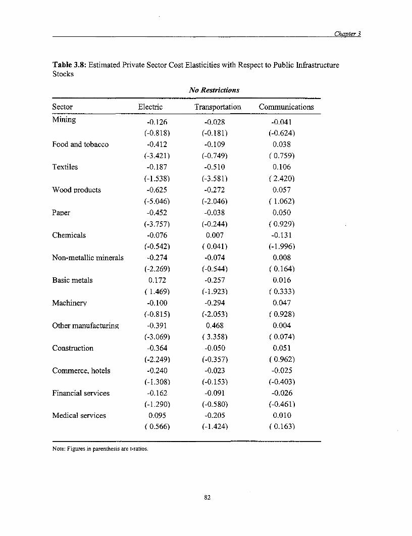
Chapter 3
Table 3.8: Estimated Private Sector Cost Elasticities with Respect to Public InfrastructureStocks
No Restrictions
Sector Electric Transportation Communications
Mining -0.126 -0.028 -0.041
(-0.818) (-0.181) (-0.624)Food and tobacco -0.412 -0.109 0.038
(-3.421) (-0.749) (0.759)
Textiles -0.187 -0.510 0.106
(-1.538) (-3.581) (2.420)
Wood products -0.625 -0.272 0.057
(-5.046) (-2.046) ( 1.062)
Paper -0.452 -0.038 0.050
(-3.757) (-0.244) ( 0.929)Chemicals -0.076 0.007 -0.131
(-0.542) (0.041) (-1.996)Non-metallic minerals -0.274 -0.074 0.008
(-2.269) (-0.544) ( 0.164)
Basic metals 0.172 -0.257 0.016
(1.469) (-1.923) ( 0.333)
Machinery -0.100 -0.294 0.047(-0.815) (-2.053) ( 0.928)
Other manufacturing -0.391 0.468 0.004
(-3.069) (3.358) (0.074)Construction -0.364 -0.050 0.051
(-2.249) (-0.357) (0.962)Commerce, hotels -0.240 -0.023 -0.025
(-1.308) (-0.153) (-0.403)
Financial services -0.162 -0.091 -0.026(-1.290) (-0.580) (-0.461)
Medical services 0.095 -0.205 0.010(0.566) (-1.424) (0.163)
Note: Figures in parenthesis are t-ratios.
82

Chapter 3
Table 3.9: Estimated Private Sector Cost Elasticities with Respect to Public InfrastructureStocks
CRS
Sector Electric Transportation Communications
Mining _n Q -01 79 n (R
(-3.002) (-0.901) ( 1.164)Food and tobacco -0.807 0.044 0.063
(-5.802) (0.251) ( 1.133)Textiles -0.276 -0.153 0.027
(-1.943) (-0.931) ( 0.570)Wood products -0.740 -0.074 0.065
(-4.972) (-0.494) ( 1.176)Paper -0.776 0.048 0.102
(-5.646) (0.248) ( 1.745)Chemicals -0.375 0.019 0.027
(-2.525) ( 0.093) (0.344)Non-metallic minerals -0.571 0.063 0.028
(-4.028) ( 0.380) (0.502)Basic metals -0.212 -0.460 0.113
(-1.624) (-2.902) (2.230)Machinery -0.446 -0.405 0.122
(-3.124) (-2.408) (2.120)Other manufacturing -0.692 0.897 -0.101
(-4.962) ( 5.634) (-2.102)Construction -0.669 0.499 -0.012
(-3.447) ( 3.287) (-0.210)Commerce, hotels -0.771 0.290 0.025
(-3.724) ( 1.668) (0.342)Financial services -0.470 -0.089 0.058
(-3.326) (-0.456) ( 0.878)Medical services -0.342 -0.121 0.105
(-1.808) (-0.700) ( 1.450)
Note: Figures in parenthesis are t-ratios.
3.45 Detailed coefficient estimates are shown in appendix D. Appendix C considersadditional specification issues, such as heteroskedasticity and autoregression. In general, theseheteroskedasticity and autoregressive consistent estimates are larger (not in absolute value) than
83

Chapter 3
the base case estimates (table 3. 10).
Table 3.10. Mean Elasticities
Category Electric Transportation Communications
Base case -0.171 -0.165 0.019
OLS, robust -0.065 0.031 0.072
OLS, random effects -0.036 -0.012 0.060
FGLS, hetero, AR(1) -0.019 -0.005 0.069
Source: Author's calculations.
3.46 This lends further support to the conclusion that the role of public infrastructure inreducing private sector costs in Mexico is modest. A notable feature of table 3.10 is that theestimated infrastructure effects are generally largest for electric infrastructure and smallest forcommunications, with the effects of transportation capital falling somewhere in the middle. Theeffects of communications infrastructure appear to be consistently positive, implying thatadditional public sector communications infrastructure increases private sector costs.
Payoffs from Additions to Infrastructure
3.47 There are several ways to try to evaluate the importance of these estimates forpolicymakers. Estimates of the optimal stocks of public infrastructure would be useful.Unfortunately, in a static context, whether the optimum is knowable is not clear. Here weestimate static elasticities, essentially the slope of the line relating changes in private sector coststo changes in infrastructure stocks. If the elasticities are negative, then naively, the estimatessuggest increasing infrastructure infinitely. An alternative approach is to consider the estimatedcosts and benefits that would be associated with different increases in infrastructure stocks. Notethat these are static calculations that ignore the shadow cost of public funds; ignore firms'reactions to infrastructure increases; and ignore financing costs, such as increases in the realinterest rate.
3.48 We consider three alternatives. The first is an illustrative elasticity calculation: what isthe result of a 1 percent increase in public infrastructure stocks? Second, what would be theeffect of an increase in infrastructure stocks of the same size as current gross investment by 60percent (to 5 percent of GDP)? All this additional investment is assumed to add to infrastructurestocks, that is, we assume that depreciation is covered separately.
84
Chapter 3
Static Costs and Benefits of Increased Infrastructure
3.49 The basic calculation is a simple comparison of the value of the estimated reductions inprivate sector costs following from an increase in public sector infrastructure stocks. The cost ofa d percentage increase in infrastructure stocks is
(4) Edgm
while the estimated benefits across the sectors 1 < j < 14 are:
(5) E E dej,,cj .m
3.50 Using our base case estimates and the 1993 values for infrastructure stocks and sectoralcosts, the estimated cost of a 1 percent increase in infrastructure would be rnxp 6.62 billions (real1980 pesos). The total benefits in private sector cost reduction would be mxp 12.35 billions (real1980 pesos). If these benefits were accrued over several years, the total would be larger. Atdepreciation and discount rates of 10 percent, the present value would be approximately mxp55.6 billion. The two scenarios based on larger expansions of public infrastructure stocks wouldbe associated with similarly larger multiperiod payoffs. Table 3.11 presents estimated costs andbenefits for the three scenarios.
Table 3.11: Static Costs and Benefits of Increased Infrastructure (real 1980 pesos, billions)
Private sector costInvestment costreuto reduction
I % increase ininfrastructure stocks 6.6 12.4
Increase by current
gross spending amount (3% GDP) 186.9 348.7Increase current amount
by 60% (5% GDP) 311.5 581.1
3.51 These are, of course, static calculations which ignore general equilibrium effects ofadditional infrastructure investments through channels such as wage and interest rates. SeeFeltenstein and Murphy (1999) for a discussion of added investments in infrastructure stocks inthe context of a general equilibrium model of the Mexican economy.
3.52 A second approach to evaluating appropriate levels of infrastructure stocks is torecognize that we estimate constant elasticities, but not constant peso changes. Therefore, ourexpression of infrastructure stocks in currency rather than physical terms allows a simple
85
Chapter 3
calculation which yields an estimate of "optimal" infrastructure stocks. For infrastructure stockm, by definition the elasticity of private sector costs with respect to stock m is:
dCl
(6) em C dG
/Gm
A static notion of optimality would require that the marginal benefits of increases in
infrastructure stock (- dCG ) be equal to the marginal costs of those increases. Infrastructure
stocks are measured in pesos and we ignore potential infrastructure production nonlinearities.Therefore the marginal cost of infrastructure increases is -1 (it costs 1 peso to increase stocks by1 peso). Then, at the optimum level of infrastructure Gm :
(7) -dC-1 =0dGm
A slight rearrangement of (7) using (6) gives:
(8) Gm * e=C
This calculation of the optimal stock implicitly assumes:
1. Total private sector cost remains constant (C is fixed)
2. Infrastructure production has constant returns to scale (marginal cost of producinginfrastructure is constant)
3. Increasing infrastructure stocks does not affect the shadow cost of government funds (which isimplicitly assumed to be zero: the cost of 1 peso is 1 peso)
4. Only current period benefits matter in calculating optimal levels.
Optimal Infrastructure Stocks
3.53 The calculated optimal infrastructure stocks are shown in Table 3.12. The calculationsare based on the mean base case elasticities for each infrastructure type with three differentelasticity assumptions for communications: -0.019 (negative of base case), 0.00, and -0.010. Thetable also includes calculations using panel elasticity estimates (feasible GLS, heteroskedasticconsistent, 1 period autoregressive structure; see Table 3.10) with the communications elasticityset to 0.00.
86

Chapter 3
Table 3.12: Optimal Infrastructure Stocks (real 1980 pesos, billions)
em Actual Gm Optimal Gm* Ratio Gm/Gm*
Base case Electric -0.171 335.0 826.8 0A41Transportation -0.165 217.4 797.8 0.27
Communications -0.019 110.0 91.9 1.20Communications 0.000 110.0 0.0
Communications -0.010 110.0 48.4 2.27
Panel Electric -0.019 335.0 91.9 3.65
Transportation -0.005 217.4 24.2 8.98
Comnmunications 0.000 110.0 0.0
3.54 Unfortunately, because the elasticity estimates are not particularly precise, neither arethe calculated levels of optimal infrastructure stocks. If the base case estimates are accurate thencurrent levels of electric and transportation infrastructure are too low; the optimal levels are 2-4times larger. However, the panel estimates suggest much lower elasticities and hence optimalinfrastructure levels. Consideration of the multi-period flow of benefits from infrastructurecapital would suggest higher optimal stocks.
Conclusions
3.55 This chapter provides estimates of the effects of public sector infrastructure stocks onprivate sector production costs. The estimates, although problematic in some respects, aregenerally quite sensible. The estimates are reasonably consistent across different empiricalmodels and, in the base case, estimated precisely. On average, the elasticity of private sectorcosts with respect to public infrastructure costs is approximately -0.10 to -0.15. Given the size ofpublic infrastructure stocks and private sector costs, these elasticity estimates suggest thatmoderate increases in public sector infrastructure stocks would be welfare improving. Theimprecise nature of the estimates suggests that caution is appropriate, however, and thecommunications and education estimates in particular should be regarded as comments on thedata rather than definitive statements about productivity.
87

Chapter 3
References
Banco de Mexico. 1995. "La Encuesta de Acervos, Depreciacion y Formacion de Capital delBanco de Mexico". Computer files.
Bemdt, E.R. 1991. The Practice of Econometrics: Classic and Contemporary. Reading, Mass.:Addison-Wesley.
Canning, D. 1998. "A Database of World Infrastructure Stocks, 1950-1995", Unpublishedworking paper.
Estados Unidos Mexicanos. 1998. Cuarto Informe de Gobierno, Annexo. Poder EjecutivoFederal: Presidencia de la Republica, Mexico.
Feltenstein, A., and Ha. 1995 "The Role of Infrastructure in Mexican Economic Reform", WorldBank Economic Review, 9(2): 287-304.
Feltenstein, A., and R. Muiphy. 1999. "Can Infrastructure Protect Against Shocks?: An Analysisof the Situation of Mexico". Unpublished working paper.
Greene, W. H. (2000). Econometric Analysis (Fourth ed.). Upper Saddle River, N.J.: PrenticeHall.
Hulten, C. R. 1996. "Infrastructure Capital and Economic Growth: How Well You Use It MayBe More Inportant Than How Much You Have." Working paper 5847, National Bureau ofEconomic Research, Cambridge, Mass.
IMNF. 1998. International Financial Statistics CD-ROM.
INEGI.1997. Cuentas Nacionales de Mexico. CD-ROM.
McGuckin, R. H., M. L. Streitsweiser, and M. E. Doms. 1996. 'The Effect of Technology Use onProductivity Growth". Working paper CES 96-2. Center for Economic Studies, U.S. CensusBureau, Washington, D.C.
Nadiri, M. I., and T. P. Mamuneas. 1994. "The Effects of Public Infrastructure and R&D Capitalon the Cost Structure and Performance of U.S. Manufacturing Industries". The Review ofEconomics and Statistics 76 (1): 22-37.
Psacharopoulos, G. 1994. "Returns to Investment in Education: A Global Update". WorldDevelopment 22(9): 1325-43.
Stiroh, K. J. 1998. "Computers, Productivity, and Input Substitution", Economic Inquiry, 36(2):175-91.
88

Chapter 3
Takayama, A. 1990. Mathematical Economics, (2nd ed.), Cambridge University Press,Cambridge, U.K.
89

Chapter 3
Appendix A.
Estimation Model Details
Let the augmented translog model from equation (2) be given by
2 2c = ao + aLwL + aKwK + bLLwL + bLKWLWK + bKKWK
+ witbiT + E wiybyi + ytb,
(9) 2 + a(y + bryy + byLywL + byKywK
+ I Pm*g + IIpjmgm wi + Ipymg.Y + u
m m i m
where the *d coefficient vectors include sector-specific effects. We gain some additionalefficiency in our estimates by noting that from Shepard's Lemma, the above specificationimplies, that the share of total cost attributable to each private factor input is
(10) SL =aL +bLKWK +bLLWL +bLYY+jPL.9 +UL
(11) S<K a' + bKKwK + bKLWL +bKYY + YPK9mm +UK
m
Furthermore, SL and SK must satisfy the adding up constraint: SL + SK. We also know that areasonable cost function must satisfy conditions such as homogeneity of degree one in inputprices, which implies that:
aL + aK =1
aLK + a. =0
aKK +aLX =0
bLy + bKy =0.
We impose these conditions, which allow us to write equation (9) as (letting r = WK and w = WL):
90

Chapter 3
* w w 2c-r =a o + a L-+ bLLW-+ bLKWLWK + bKKr
r r
w+ aTt + bLTt ±+ bTy yt
(12) r2 W+a Yy+byyy +byLY-
r
+ p*mgm +YpLing. n+JPymgiy+Um m ~ ~~~ m
(subject to bKK =bLL)
and
(13) SL =a*L +btL-+bLyy+bLTt+PL.9. +ULr m
In addition to the above, a constant degree of homogeneity in output requires
bLY = bKY = 0
byy =byr =0
bYE =bn =byC =YD =0
where the infrastructure subscripts are E for electricity, R for transportation, C forcommunications, and D for education. Finally, CRS further implies that
(14) ay =1.
In our estimation, we begin with equations (12) and (13), impose the appropriate conditions, andestimate the model parameters in a seemingly unrelated regression framework. This shouldprovide reasonable statistical properties, and the estimates should be invariant to the choice ofwhich cost share equation to delete (see Berndt 1991; Nadiri and Mamuneas 1994).
91

Chapter 3
Appendix B
Specification Issues
3.56 There are several econometric specification issues which we need to consider. A majorconcern is that due to the panel nature of the data (14 sectors of the economy over 34 years), thedisturbance terms in the empirical models may be characterized by heteroskedasticity,autoregression, or both.
3.57 We estimate the basic model (cost equation only) for several alternative specifications.Below (Tables -) are elasticity estimates for three of these:
1. Ordinary least squares (OLS) with robust standard errors (Table 3.13)
2. OLS with random effects (Table 3.14)
3. Feasible generalized least squares (FGLS) with cross-panel heteroskedasticity and withinpanel one period autoregression (Table 3.15)
3.58 If the relationship between private sector costs and public infrastructure is adequatelydescribed by equation (2) except for the error term having a sector specific variance, then theOLS with robust standard errors model will generate consistent estimates of the elasticities andtheir standard errors.
3.59 The random effects estimates allow for sector specific and common error components.That is, we allow the error term to take the form v, + uit; vi is a sector specific disturbance term,while ui, is a sector and period specific term. A Breusch-Pagan test of whether or not the sectorspecific terms are 0 rejects the null hypothesis that they are, suggesting that the random effectsspecification is to be preferred (p-value=0.00). A Hausman test of the appropriateness of therandom effects model relative to a fixed effects alternative (are the subset of coefficientscommon to the random effects and related fixed effects models systematically different whenthey should not be) does not lead us to reject the null hypothesis (p-value = 1.00) that the randomeffects model is appropriate or that the subset of coefficients does not differ systematically (seeGreene (2000) for a discussion of these tests).
3.60 The FGLS estimates allow for cross-sector heteroskedasticity and within sector oneperiod autoregression (common across sectors). Assuming that our sector specific variance andcross-sector one period auto-correlation specification is correct, the FGLS estimates shouldprovide efficient estimates of the standard errors. Think of the FGLS estimates as allowing for(some) sectoral and temporal variation in the disturbance terms.
3.61 All of these models attempt to more carefully construct estimates of the non-systematicpart of the basic cost equation. We also considered several other models with variousspecifications of the way disturbance terms might be related across sectors and time (not reportedhere); none of these models produced compelling estimates.
92

Chapter 3
Appendix C.
The Data
Table 3.13: OLS panel elasticities (robust t-ratios in ('s)
Sector Electric Transportation Communication
Mining n1 M() n 06 n 006
(1.562) ( 0.166) ( 1.665)Food and tobacco -0.107 0.048 0.062
(-1.425) ( 1.144) ( 2.804)Textiles -0.081 -0.147 0.110
(-0.806) (-2.035) ( 3.991)Wood products -0.328 0.023 0.103
(-5.882) ( 0.247) ( 3.533)Paper -0.123 0.070 0.071
(-1.402) ( 1.154) (2.670)Chemicals -0.022 0.067 0.047
(-0.148) ( 0.942) ( 0.941)Non-metallic minerals -0.130 0.054 0.071
(-2.202) ( 0.892) ( 3.044)Basic metals 0.160 0.105 0.023
(1.812) ( 1.056) ( 0.865)Machinery 0.056 -0.087 0.075
(1.061) (-0.828) ( 3.729)Other manufacturing -0.093 0.000 0.116
(-0.900) (0.002) ( 3.383)Construction -0.096 0.062 0.067
(-1.295) (0.738) ( 3.518)Commerce, hotels -0.075 0.011 0.082
(-0.613) ('0.125) (2.437)Financial services -0.075 0.083 0.047
(-0.841) (2.054) (1.482)Medical services -0.156 0.132 0.075
(-1.121) (2.306) (1.873)
93
Chapter 3
Table 3.14: OLS random effects elasticities (t-ratios in ('s)
Sector Electric Transportation CommunicationsMining 0.211 -0.044 0.055
(1.841) (-0.416) (1.096)Food and tobacco -0.084 0.019 0.049
(-0.966) (0.191) (1.338)Textiles -0.006 -0.131 0.066
(-0.068) (-1.433) (2.138)Wood products -0.297 -0.086 0.086
(-3.307) (-1.015) (2.155)Paper -0.082 -0.002 0.063
(-0.942) (-0.022) (1.583)Chemicals -0.050 -0.007 0.080
(-0.483) (-0.058) (1.600)
Non-metallic minerals -0.088 -0.027 0.061(-1.010) (-0.309) (1.620)
Basic metals 0.195 0.082 0.007( 2.278) (0.950) (0.199)
Machinerv 0.057 -0.101 0.064( 0.639) (-1.050) (1.728)
Other manufacturina -0.001 -0.046 0.064(-0.010) (-0.510) ( 1.789)
Construction -0.073 0.064 0.035
(-0.598) (0.706) ( 0.893)Commerce, hotels -0.073 -0.025 0.081
(-0.522) (-0.249) ( 1.706)Financial services -0.072 0.047 0.052
(-0.792) ( 0.435) ( 1.213)Medical services -0.140 0.095 0.080
(-1.102) ( 0.988) ( 1.626)
94

Chapter 3
Table 3.15: FGLS elasticities - hetero, ARI (t-ratios in ('s)
Sector Electric Transportation CommunicationsMining 0.176 -0(039 0.070
(1.212) (-0.275) (1.675)Food and tobacco -0.069 0.006 0.059
(-1.668) (0.138) (3.525)Textiles 0.073 -0.135 0.074
(1.696) (-3.205) (5.127)Wood products -0.249 -0.101 0.099
(-4.225) (-1.903) ( 4.380)Paper -0.087 0.005 0.073
(-1.727) ( 0.083) ( 3.505)Chemicals -0.105 0.005 0.084
(-1.971) ( 0.098) ( 3.579)Non-metallic minerals -0.068 -0.013 0.069
(-1.362) (-0.264) ( 3.480)Basic metals 0.228 0.158 0.004
( 3.244) (2.227) ( 0.146)Machinery 0.087 -0.037 0.061
( 1.747) (-0.706) ( 3.170)Other manufacturing 0.082 -0.028 0.070
( 1.253) (-0.449) (3.001)Construction -0.012 0.031 0.049
(-0.209) (0.719) ( 2.672)Commerce, hotels -0.047 -0.040 0.091
(-0.617) (-0.734) ( 3.913)Financial services -0.104 0.049 0.063
(-3.487) ( 2.238) ( 3.866)Medical services -0.165 0.068 0.095
(-2.261) ( 1.231) ( 3.800)
3.62 The analysis requires several pieces of data, all on an annual basis. The sources of thesedata are described here. Note that one of the primary sources for our data, INEGI (1997), for
95

Chapter 3
some variables presents two separate series of data, one for 1970-84 and one for 1980-93.Unfortunately, these series are not always consistent. Where the series are inconsistent, the laterseries are ordinarily combined with the growth rates implied by the earlier series.
Gross Output
3.63 The needed measure of sectoral output is gross output, not value added. The INEGI(1997) accounts do not include a consistent time series of gross output for 1960-93. Thereforethe data used in this paper are constructed as follows.
3.64 For the 1980-93 period, constant price (in 1980 new pesos) gross production figures andimplicit price deflators (base 1980) are available for the nine major sectors of the economy, aswell as for the major divisions of the manufacturing sector that are of interest. These data arefound in the directories
inegi / cuentas / cn / scnm / ser8O_93 / cue_prod / gd_j / total /
for each major sectorj. This gives us pb, 1980 S t < 1993.
3.65 For the 1970-84 period, constant price (in 1970 pesos) gross production figures andimplicit price deflators (base 1970) are available for all the relevant sectors of the economy.There does not appear to be a ready conversion rate from 1970 pesos to 1980 pesos. These dataare found in the directories
inegi / cuentas / cn / scnm / ser7O_84 / cue_prod / gd_j / total /
for each major sectorj.
3.66 To calculate pb for 1970-79 in 1980 pesos, the data selected include gross output (pb)
and value added (pib). These figures are used to calculate the ratio of gross product to valueadded: This ratio is then multiplied by pib in 1980 pesos. For each year, gross product for eachsector in 1980 pesos is based on real (1980 pesos) value added by sector and the ratio of pb topib in 1970 pesos:
(15) PbIg8o =pib,98o x pb1 970 J for 1970< t • 1979.p1b5970pt
This gives us pb,, 1970 < t < 1993.
96

Chapter 3
For the period 1960-85, gross production (pb) is reported only for the nine major sectors of theeconomy and only in 1970 pesos.
The pb figures in 1980 pesos are calculated as follows:
* From the files in inegi/cuentas/cn/scnm/ser_his/ser60_85/oyu/pb and its subsidiarydirectories, we calculate the growth rates (real 1970 pesos) in pb by sector for each year1960-70.
* Beginning with the 1970 constant peso (1980 pesos) gross output figures calculated above(based on the ratio of pb to pib), we work back to 1960 using the growth rates for 1970 pesobased figures. For the nine Divisions of the manufacturing sector (sectors two to ten in thischapter), we use the overall manufacturing growth rate, because the disaggregated Divisiondata are not available.
In summary, the 1960-93 gross output (pb) figures are derived as follows:
* 1980-93: from (INEGI 1997) published tables
* 1970-84: from pib in 1980 new pesos data and the ratio of pb to pib for 1970 peso data
* 1960-69: from the calculated 1970 value of pb in 1980 pesos and the growth rates of 1970peso pb figures.
Production Cost
Production cost is measured by real (1980 prices) value added, or Producto Interno Bruto (pib).INEGI (1997) reports these figures for 1960-93 in directories
inegi/cuentas/cn/scnm/ser_his/ser6O_93/pib (nine major sectors)
and
inegi/cuentas/cn/scnm/ser_his/ser6O_93/pib/gd_3 (nine manufacturing sectors)
The data are copied (with some rearrangement) directly from the (INEGI 1997) files.
Value added is also reported for major sector 1, Agropecuario, Silvicultura y Pesca, which weignore because there are no capital accounts available for the agriculture sector. To the extentthat the agriculture sector is dominated by small-scale, local farming, this will not materiallychange our results as long as these producers are unlikely to make much use of governmentprovided infrastructure of the types we consider.
97

Chapter 3
Factor Payments
3.67 The two private inputs are labor and capital. We take two approaches to calculatingfactor payments. First, we take sector-specific factor prices (mean wages, Treasury bill rate) andmultiply by sector-specific factor usage (employment, net capital stock). Second, we use nationalincome accounts estimates of wage payments and payments to owners of capital. Our preferredmeasures are those from the national income accounts.
Wage Rates
3.68 For labor, INEGI (1997) reports mean nominal remuneration for 1980-93 and 1970-84by sector (nine major sectors and nine divisions of manufacturing). The 1980-93 figures areconverted to real 1980 pesos using the implicit price deflators for gross output (from the samedirectories). The 1980s data is in datasets wage. dta (nominal data) and rwage. dta (real data) inthe scrrn/ser80_93/cue_prod directory.
3.69 INEGI (1997) also reports nominal 1970 peso figures for 1970-84. These are convertedto real 1970 pesos using the appropriate implicit price deflators. The real 1970 figures are used tocalculate growth rates, which are then successively applied (beginning with real 1980 figures) togenerate real mean wages back to 1970. The 1970s figures are contained in the datasets nom-
wages. dta and rwageg. dta in the scnm/ser70_84/cue_prod directory.
3.70 For 1960-69 we construct three different series based on potential wage paths. In allcases, we work from our constructed 1970 figures, and from 1970 we calculate the 1960-69values assuming that wages grew as follows:
- GDP growth: wages in all sectors grow at the same rate as the growth rate of the Mexicaneconomy
* pib growth: wages in each sector grow at the same rate as value added in that sector
3 No growth: w, = w, , 1960 < t < 1969.
Our base case is that wages grow at the same rate as overall GDP.
Interest Rates
3.71 The interest rate used is the Mexican Treasury Bill rate. This is admittedly crude, but asour primary concem (for purposes of estimation) is variation, it is not too bad. For 1978-93 therate used is the one reported in IFS (1998). This series has a gap in 1986. For 1986 we estimatethe Treasury bill rate based on a OLS regression of the rate on the time deposit rate (alsoreported in IFS 1998) for 1978-93 (excluding 1986). The estimated relationship, which has an F-statistic of F(1,13) = 2137.77 (p = 0.0000), is
98

Chapter 3
(16) t = 0.211 + 1.067d
(1.014) (0.023)
3.72 For the years prior to 1978, we estimate the Treasury bill rate as follows. The 1977 rateis estimated using the 1977 time deposit rate and the estimated equation (16). Nominal interestrates are converted to real interest rates by subtracting the annual growth in the consumer priceindex. Prior to 1977, we calculate the Mexican Treasury bill rate based on an assumed paritybetween U.S. and Mexican rates:
(17) rM,t XM,tX US,t
where the subscripts M and US refer to Mexico and the United States, respectively. Real interestrates are indicated by r, nominal interest rates by R, the nominal exchange rate with the USdollar by x, and price indices by I. All data are taken from IFS (1998).
Employment
3.73 We use sectoral employment to calculate total labor costs. For 1980-93 we use sectoremployment from INEGI (1997). For 1970-79, we use the growth rates of employmentcalculated from the employment data presented for 1970-83 to extend the 1980 figures backannually to 1970. For 1960-69 we use the sector growth rates of pib or value added to extendthe 1970 figures back to 1960.
Private Capital Stocks
3.74 Private sector capital figures are from the banco data. The tables indata/banco/capi tal -constant were edited, and then aggregated into the appropriate industrysectors.
National Income Accounts
3.75 For 1970-93 period, INEGI (1997) reports the disposition of pib into: Remuneracion DeAsalariados, Impuestos Indirectos Menos Subsidios, and Excedente Bruto De Operacion. Weignore taxes and indirect subsidies and calculate labor and capital shares on the basis of the wageand surplus flows only.
99

Chapter 3
For 1970-84 figures are available in 1970 pesos. To construct 1980 new peso equivalents, wecalculate real (1970 peso) flows using the sectoral implicit price deflators and then calculate thereal growth rates. Then we estimate the 1970-79 figures using the real 1980 (1980 new pesosbasis) figures and the 1970-80 growth rates in real 1970 peso terms.
For 1960-69 we assume that labor payments grew at the rate of sectoral pib, while payments tocapital grew at the rate of sectoral net capital stocks.
Government Infrastructure
3.76 We use the net capital stocks of three sectors of the economy, electricity (Rama 61contained in major sector 5), transportation (Rama 64 contained in major sector 7), andcommunications (Rama 65 contained in major sector 7) as our measures of governmentinfrastructure. The transportation and communications figures are presented in Banco de Mexico(1995). We use total net capital for each of these sectors as our measures of nationalinfrastructure stocks.
3.77 Comparable figures have been published for the electric sector, but are not currentlyavailable. We construct net capital stock series for electricity as described here. Banco deMexico (1995) presents both real (1980 new pesos) and nominal capital stock figures.
The real capital stock series for electricity is constructed in stages, as follows:
* Previous Banco de Mexico publications present net capital for sector 61 in 1970 pesos for1960-90.
- We calculate the ratio of real 1980 pesos to real 1970 pesos using implicit price deflators formajor sector 5. INEGI (1997) presents 1970-denominated gross output pb for major sector(which includes sector 61) for 1970-84 and 1980-denominated gross output for 1980-93.
* These ratios are used to convert the 1970-denominated net capital figures for 1980-84 to1980-denominated net capital figures.
* The growth rates in the 1970-denominated net capital figures are used to extend the 1980figure back to 1960 and to extend the 1984 figure up through 1990.
* Estados Unidos Mexicanos (1998) presents estimates of total infrastructure (in megawatts) inthe electric industry for 1988-98. The growth rates in these figures are used to extend the1990 estimates calculated above forward until 1993.
Likewise, the nominal net capital stock series for the electric infrastructure is constructed instages as follows:
* The real (1970 pesos) capital stocks for four types of capital (Edificios, Construcciones eInstalaciones, Maquinaria y Equipo de Operacion, Equipo de Transporte, and Mobiliario y
100
Chapter 3
Equipo de Oficina) in Rama 61 are presented in the previous Banco de Mexico tables. Aseparate file (PRE4 9937.. PRN) presents implicit price deflators for these series. These deflatorsare used to generate nominal capital stock figures for each series, which are then summed toprovided total net capital for 1960-90.
* To convert the 1970 pesos to 1980 pesos, we calculate the ratio of nominal pb (1970 pesos)to nominal pb (1980 pesos) for Rama 61 for 1980-84 and use the average of the ratios forthese five years as our conversion factor (1.325429).
* For the years 1991-93, we calculate real growth (see above) and price level growth for eachyear. The nominal figures are calculated as the product of the prior year's nominal figuretimes one plus the sum of real and price level growth. Price level growth is estimated byusing the implicit price level changes of total net capital in Rama 64 (communications). Thederived growth rates are shown in table 3.16
Table 3.16: Growth rates used for nominal electricity infrastructure
Real Price Total
1991 0.0639 0.2014 0.2653
1992 0.0126 0.1467 0.1593
1993 0.0685 -0.0602 0.2633
101

Chapter 3
Appendix DRegression Results
Coefficient estimates from various specifications are as follows:
Table 3.17: Coefficient estimates
Base With Education 1960-1993 No restrictions CRSCost aL 26.016 25.709 52.041 27.308 1.385
(2.369) (2.393) (2.498) (4.748) (1.164)bLL -0.095 -0.093 -0.121 -0.102 -0.062
(0.007) (0.007) (0.007) (0.006) (0.008)bKK -0.095 -0.093 -0.121 -0.102 -0.062
(0.007) (0.007) (0.007) (0.006) (0.008)ay -15.608 -16.925 3.265 -16.475
(1.374) (1.502) (1.039) (3.465)byy 0.021
(0.157)bLy 0.011
(0.052)aT 0.100 0.109 0.188 0.060 0.008
(0.008) (0.009) (0.009) (0.024) (0.002)bLT -0.012 -0.012 -0.025 -0.013 -0.0001
(0.001) (0.001) (0.001) (0.003) (0.001)byT 0.004
(0.001)
PE -15.196 -15.865 -1.254 -11.281 1.074(2.519) (2.951) (0.307) (3.042) (2.504)
PLE -0.162(0.066)
PYE 1.241 1.326 0.108 0.999 -0.132(0.205) (0.240) (0.028) (0.242) (0.200)
PR -4.127 -5.269 4.062 -2.507 -3.016(2.282) (2.150) (1.159) (3.172) (2.739)
pLR 0.239(0.056)
PYR 0.330 0.402 -0.370 0.073 0.232
(0.185) (0.175) (0.097) (0.249) (0.223)
PC 3.190 4.685 -1.047 4.409 -0.129(0.926) (1.233) (0.320) (1.026) (1.053)
PLC -0.083(0.036)
PYc -0.262 -0.387 0.092 -0.318 0.017(0.079) (0.105) (0.027) (0.085) (0.090)
PD 2.100(9.227)
PYD -0.079(0.752)
aO (dropped) (dropped) -403.097 (dropped) (dropped)(22.920)
102
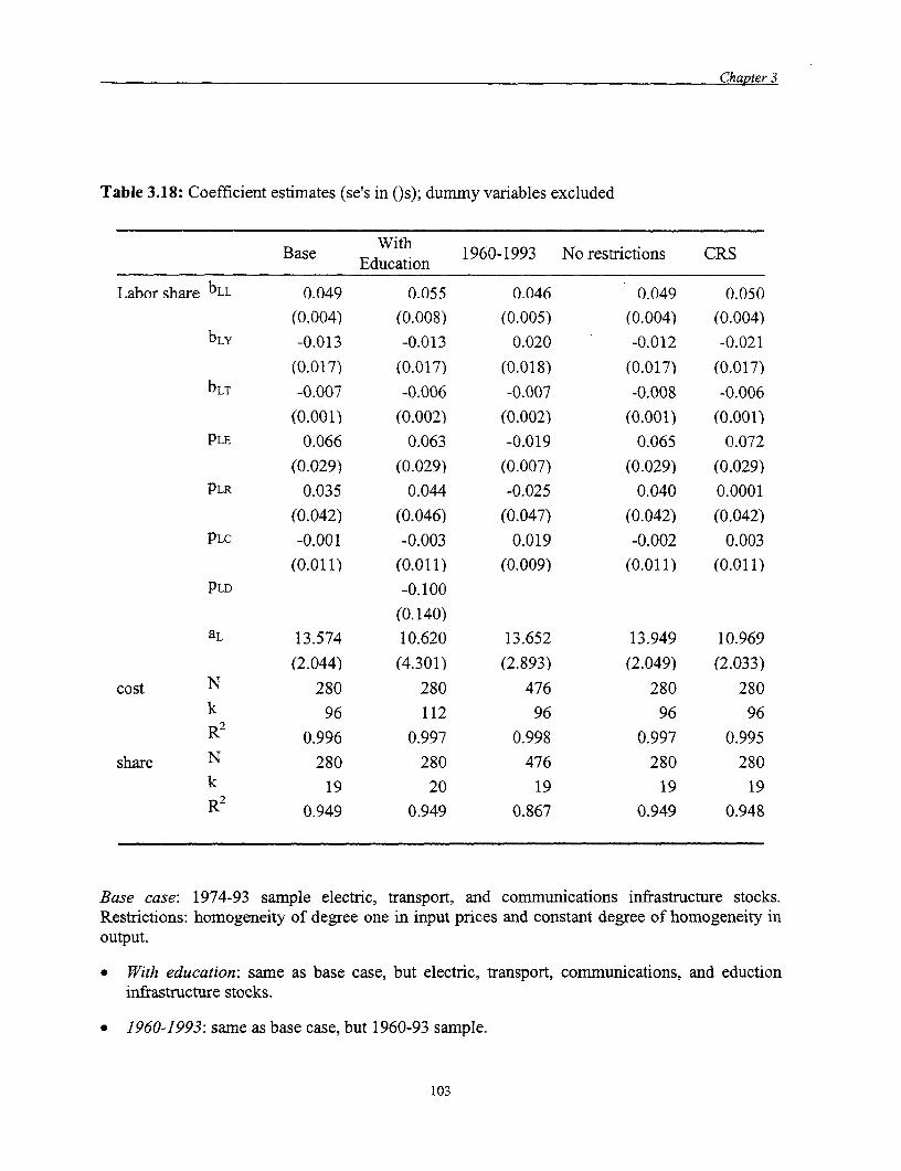
Chapter 3
Table 3.18: Coefficient estimates (se's in (s); dummy variables excluded
Base With 1960-1993 No restrictions CRSEducation
Labor share bLL 0.049 0.055 0.046 0.049 0.050
(0.004) (0.008) (0.005) (0.004) (0.004)
bLy -0.013 -0.013 0.020 -0.012 -0.021
(0.017) (0.017) (0.018) (0.017) (0.017)bLT -0.007 -0.006 -0.007 -0.008 -0.006
(0.001) (0.002) (0.002) (0.001) (0.001)PLE 0.066 0.063 -0.019 0.065 0.072
(0.029) (0.029) (0.007) (0.029) (0.029)PLR 0.035 0.044 -0.025 0.040 0.0001
(0.042) (0.046) (0.047) (0.042) (0.042)PLC -0.001 -0.003 0.019 -0.002 0.003
(0.011) (0.011) (0.009) (0.011) (0.011)PLD -0.100
(0.140)
aL 13.574 10.620 13.652 13.949 10.969(2.044) (4.301) (2.893) (2.049) (2.033)
cost N 280 280 476 280 280k 96 112 96 96 96
R2 0.996 0.997 0.998 0.997 0.995share N 280 280 476 280 280
k 19 20 19 19 19R2 0.949 0.949 0.867 0.949 0.948
Base case: 1974-93 sample electric, transport, and commnunications infrastructure stocks.Restrictions: homogeneity of degree one in input prices and constant degree of homogeneity inoutput.
* With education: same as base case, but electric, transport, communications, and eductioninfrastructure stocks.
* 1960-1993: same as base case, but 1960-93 sample.
103

Chapter 3
* No restrictions: same as base case, but the restrictions are only homogeneity of degree one ininput prices.
* CRS: same as base case, but the restrictions are homogeneity of degree one in input pricesand constant returns to scale in output.
104


4FISCAL IMPACT OF CONTINGENT LLIBILITIES:
THE CASE OF MEXICO
4.1 One result of the financial crises affecting Asia, Latin America and other emergingeconomies over the recent past has been a renewed emphasis on the fiscal risks (liabilities)governments' face and means to quantify and mollify such risks. In general, liabilities can beeither contingent or direct. Contingent liabilities are defined as "obligations that may or may notcome due, depending on whether particular events occur. The probability of their occurrencemay be exogenous to government policies (for example, if they are related to natural disasters) orendogenous (for example, if government programs create moral hazard)." In contrast, directliabilities are defined as "obligations whose outcome is predictable."
4.2 Delineating further, "Explicit liabilities are specific obligations, created by law orcontract, that governments must settle. Implicit liabilities represent moral obligations or burdensthat, although not legally binding, are likely to be borne by govermnents because of publicexpectations or political pressures."'
4.3 A Fiscal Risk Matrix2 developed by the World Bank provides an efficient means ofcategorizing these risks:
Table 4.1 Fiscal Risk Matrix
Liabilities Direct (obligation in any event) Contingent (obligation if a particular event occurs)Explicit * Foreign and domnestic sovereign * State guarantees for nonsovereign borrowing and obligations issued to
borrowing (loans contracted and subnational Governments and pubhc and private sector entities (developrnentGovernment liability as securities issued by central banks)recognized by a law or Government) . Umbrella state guarantees for various types of loans (mortgage loans, studentcontract * Budgetary expenditures loans, agriculture loans, small business loans)
Budgetary expenditures legally binding * Trade and exchange rate guarantees issued by the statein the long termn (civil servants' salaries * State guarantees on private invesrnentsand pensions) * State insurance schemes (deposit insurance, income from private pension
funds, crop insurance, flood insurance, war-risk insurance)
Implicit * Future public pensions (as opposed to * Defaults of subnational Government or public or private entities oncivil service pensions), if not required nongusranteed debt and other obligations
A mnoral obligation of by law * Cleanup of liabilities of entities being privatizedGovermnent that reflects * Social security schemes, if not required * Banking failure (support beyond state insurance)public and interest-group by law . Failwe of a nonguaranteed pension fund, employment fund, or social securitypressures * Future health care financing, if not fund (protection of small investors)
required by law . Default of central bank on its obligations (foreign exchange contracts,Future recurrent costs of public currency defense, balance of paynments stability)investments . Bailouts following a reversal in private capital flows
Environmental recovery, disaster relief, nilitary financing
Polackova, Hana; Contingent Government Liabilities: A Hidden Fiscal Risk; Finance & Development, March 1999.2 Ibid.

Chapter 4
4.4 This chapter addresses the measurement of contingent liabilities for Mexico within thegovernment's traditional budget accounting framework. The key research problem is to identify,quantify, and understand the future fiscal risks posed by the government's contingent liabilities.The lack of a unified measure of contingent liabilities makes difficult the assessment of thesustainability of the fiscal policy. Therefore, the objective of the study is to provide an overviewof the problem in Mexico and suggest an analytical construct for assessing the magnitude of theproblem.
4.5 Prior to 1995, the budgetary treatment of contingent liabilities was never considered inMexico an issue for fiscal sustainability, nor was it viewed as an important determinant of publicsector debt dynamics. The financial crisis of 1995 dramatically changed this view. The crisisresulted in the financial insolvency of the private banking system, the open recognition of theproblems inherent in the pay-as-you-go social security system, the undercapitalization of severaldevelopment banks, and the financial distress of many private firms among which those involvedin providing quasi-public goods (such as highways).
4.6 Since the 1995 financial crisis, fiscal sustainability has been at the forefront of the policyagenda. The fiscal impact of the currency crisis prompted the government to increase the valueadded tax rate from 10 percent to 15 percent in 1995. The restructuring of the pension system,the declining intemational oil prices and the costs of resolving the 1997-98 banking crisis haveput additional pressures on Mexico's fiscal accounts. As a result, the government recentlyrequested a further raise in indirect taxes and an increase in indirect personal income taxes.Congress approved only the latter for fiscal year 1999. Thus, projections indicate that thebudgetary primary surplus for 1999 will be the second lowest since 1987. The surplus isexpected to be 2.7 percent of gross domestic product (GDP), a full 5 percentage points lowerthan the record 7.7 percent surplus posted in 1989.
4.7 A recent study by Solis and Villag6mez (1999) focuses on the issue of fiscalsustainability in this context. Using various tests of the government's present value borrowingconstraint, they conclude that for the period 1988-97 there is no basis for expecting violation ofthe constraint. In other words, the current fiscal policy is sustainable. One limitation on the Solisand Villag6mez study, acknowledged by the authors, is that they did not consider off-budgetitems such as contingent liabilities.
4.8 The main conclusion of this chapter is that contingent liabilities are a significantgovernment liability, and the amount is well beyond official estimates. Rough estimates indicatethat the fiscal deficit projected for 1999 needs to be adjusted significantly, which should put theissue of fiscal sustainability on the policy agenda for the foreseeable future. Given the size of thecontingent liabilities, monitoring the accrual accounting indicators is important. Accountingsystems within federal agencies must be redesigned to ensure the transparency of their programs'fiscal costs. Such information would provide the right incentives to reduce potential costs of thecontingent liabilities to taxpayers.
4.9 This chapter starts by describing the coverage of the study. Given the abundantmeasurement problems, it next provides general qualifications, before moving on to anexplanation of the methodology used. Subsequent sections discuss each contingent liability, with
106

Chapter 4
no attempt to measure the potential social benefits of the government's programs. The chapterconcludes with an estimate of the fiscal cost of the contingent liabilities before presenting severalpolicy recommendations.
Coverage of the Study
4.10 Table 4.2 lists the various contingent liabilities with major fiscal risk. For the sake ofconvenience, government contingent liabilities will be referred collectively as the FederalInsurance Programs (FIPs). As indicated, these liabilities include explicit obligations such asdeposit insurance, pension benefits,3 and various loan guarantees, as well as implicit obligations,such as rescuing development banks and the private firms involved in providing such publicgoods as basic infrastructure.
Table 4.2. Federal Insurance Programs with Potential Fiscal Risks
Insurance program Type of obligation Institutions involved Observations
Pension plan: retirement Required by law IMSS (mostly for private Current fiscal outlaysbenefits and hospital sector employees) and for the two institutionsexpenditures ISSSTE (for civil servants) are in the budget
Deposits in the private Required by law Private banks, National Current fiscal outlaysbanking system Banking Commission, and for FOBAPROA are in
the trust fund FOBAPROA the budget
Loan guarantees and Contractual obligation Private banks, development No fiscal outlays are indirect loans banks, and the central bank the budget for default
cases
Default of private firmns Not required by law Development banks and No fiscal outlays are inand no contractual private firms involved in the the budget for defaultobligation provision of infrastructure cases
4.11 Two important things omitted in this study: first, the expected effects on the fiscalaccounts of the debt restructuring of states and municipalities as a result of 1995 crisis; andsecond, the analysis of the pensions of subnational governmental institutions. Assessing theseareas is difficult because of incomplete and inconsistent data, however these are clearlycontingent liabilities at the Federal level. Table 4.3 below presents estimates of the debt stock atthe state level only (very limited data exists at the municipal level). Note the disturbing trends inboth the size and the concentration of the debt at the state level; the debt of the Federal District,State of Mexico, Nuevo Le6n has grown from 33 percent in 1994 to 65 percent of the totaloutstanding in 1998.
3 This point deserves clarification. Federal Pension liabilities are not strictly speaking a contingent liability, but adirect liability, and barring default, those payments will be made. Subnational pension liabilities are contingentliabilities at the Federal level.
107

Chapter 4
Table 4.3 State Govemment Debt
rnillion of pesos share in the total outstanding debt of the federationState 1994 1995 1996 1997 1998 1994 1995 1996 1997 1998Aguascalientes 364.0 307.5 339.2 287.0 227.3 1.4 0.8 0.6 0.5 0.3Baja Cal. Norte 999.6 960.3 1214.3 1380.3 1528.5 3.7 2.4 2.3 2.4 2.1Baja Cal. Sur 304.3 296.8 350.6 450.4 452.8 1.1 0.7 0.7 0.8 0.6Campeche 499.0 460.9 518.1 419.2 228.4 1.9 1.2 1.0 0.7 0.3Coahuila 515.5 926.0 1116.4 593.5 666.2 1.9 2.3 2.1 1.0 0.9Colima 191.9 263.4 291.0 237.1 192.5 0.7 0.7 0.6 0.4 0.3Chiapas 1024.7 992.0 1088.1 961.6 931.8 3.8 2.5 2.1 1.6 1.3Chihuahua 921.5 1215.2 1538.5 1689.1 1593.4 3.4 3.0 2.9 2.9 2.2Durango 552.0 462.3 606.7 713.9 806.9 2.0 1.2 1.2 1.2 1.1Guanajuato 405.6 411.7 464.5 517.2 569.1 1.5 1.0 0.9 0.9 0.8Guerrero 515.8 858.2 983.7 1168.5 1255.1 1.9 2.2 1.9 2.0 1.8Hidalgo 22.6 14.2 16.1 12.7 10.8 0.1 0.0 0.0 0.0 0.0Jalisco 2811.6 3371.9 3876.2 4006.9 4418.4 10.4 8.5 7.4 6.8 6.2Mexico 4843.0 8643.9 13396.7 16609.5 18574.9 18.0 21.7 25.4 28.4 25.9Michoacan 249.6 256.2 251.8 216.0 251.6 0.9 0.6 0.5 0.4 0.4Morelos 144.3 232.7 244.1 365.2 399.5 0.5 0.6 0.5 0.6 0.6Nayarit 222.6 187.6 178:0 115.2 104.6 0.8 0.5 0.3 0.2 0.1Nuevo Leon 2348.4 6427.4 5463.5 6706.6 7470.5 8.7 16.1 10.4 11.5 10.4Oaxaca 260.3 147.0 192.9 202.8 261.4 1.0 0.4 0.4 0.3 0.4Puebla 156.1 321.4 308.7 351.7 478.1 0.6 0.8 0.6 0.6 0.7Queretaro 1282.8 1090.0 1016.8 1061.1 1163.3 4.8 2.7 1.9 1.8 1.6Quintana Roo 450.3 643.4 740.3 842.5 1009.9 1.7 1.6 1.4 1.4 1.4San Luis Potosi 345.9 426.3 543.9 599.4 708.7 1.3 1.1 1.0 1.0 1.0Sinaloa 873.6 1337.6 1677.4 1931.2 2212.9 3.2 3.4 3.2 3.3 3.1Sonora 3150.1 4869.4 6085.5 3672.4 3990.7 11.7 12.2 11.6 6.3 5.6Tabasco 518.1 343.3 411.1 431.9 598.6 1.9 0.9 0.8 0.7 0.8Tamnaulipas 368.5 531.9 363.8 315.2 279.7 1.4 1.3 0.7 0.5 0.4Tlaxcala 136.2 52.7 0.0 0.0 0.0 0.5 0.1 0.0 0.0 0.0Veracruz 348.3 379.4 262.3 78.8 52.2 1.3 1.0 0.5 0.1 0.1Yucatan 305.1 288.1 320.9 372.2 290.1 1.1 0.7 0.6 0.6 0.4Zacatecas 123.9 380.9 468.8 235.9 136.2 0.5 1.0 0.9 0.4 0.2SUB TOTAL 25255.2 37099.6 44329.9 46545.0 50864.1 93.7 93.0 84.2 79.6 71.0Fed. District 1703.4 2772.5 8322.3 11958.2 20763.2 6.3 7.0 15.8 20.4 29.0TOTAL 26958.6 39872.1 52652.2 58503.2 71627.3 100.0 100.0 100.0 100.0 100.0
Source: SHCP.
108

Chapter 4
4.12 An additional piece missing from the analysis addressed in this review is the pensionliabilities of the states and municipalities. Table 4.4 below presents the very limited publicinfornation available on state-level pension liabilities. A cursory review of the available datareveals a significant problem on the horizon.
TABLE 4.4: State Government Pension Liabilities: 1997 (millions of pesos)
State Actuarial Deficit Reserves Year of Sufficiencv No. of Pensioners No. of WorkersAguascalientes 1,019 2010 868 11,032Baja Cal. Norte 11,987 1999 1,158 10,912Baja Cal. Sur no plan No plan no plan no planCampeche 1,320 NA NA NACoahuila 1,051 2022 700 7,895Coahuila 5,695 2001 2,838 17,173Colima NA in deficit 668 4,125Chiapas 9,837 2011 1,406 19,777Chihuahua 18,602 2000 6,348 27,546Durango NA 1999 1,741 12,046Guanajuato NA in deficit 2,917 33,889Guerrero NA 2000 1,191 13,148Hidalgo NA NA 998 7,610Jalisco 39,814 2011 4,432 85,219Mexico NA 2009 11,248 185,739Michoacan 60 2006 1,347 21,747Morelos NA NA 1,424 10,457Nayarit NA 2050 904 6,878Nuevo Leon NA NA 7,075 34,911Oaxaca NA 2002 919 9,279Puebla NA 2005-2008 2,483 36,806Queretaro NA NA 353 8,597
Quintana Roo no plan No plan no plan no planSan Luis Potosi 6,140 2006 1,140 13,871Sinaloa NA NA 1,013 8,905Sinaloa 5,483 in deficit 2,212 10,959Sonora 3,035 in deficit 4,202 34,226Tabasco NA 2009 1,155 52,001Tamaulipas 2,471 2018 2,085 18,159Tlaxcala 1,426 2013 495 7,503Veracruz 45,805 1999 10,893 58,431Yucatan NA 2015 2,549 17,690Zacatecas 1,320 2020 2,375 45,421
SUB TOTAL 155,065 79,137 831,952Fed. District 11,663 in deficit 11,732 57,891
TOTAL 166,728 90,869 889,843Note: Coahuila & Sinaloa have separate pension systems for state workers and teachers.Source: SHCP.
109
Chapter 4
Government Accounting Issues
4.13 In Mexico, government accounts are reported using the traditional cash approach, whichrecognizes receipts, cash outlays, and borrowing at the time of remittance. Several authors (Bohn1992, Boskin et al, 1987) have criticized the use of cash accounting; the buildup in thegovernment's contingent liabilities suggests a need for accrual accounting, whereby expenses arerecorded when the liability is incurred regardless of when actual payment is made.
4.14 In the case of insurance programs already considered in the budget, their explicit cashoutlays need to be monitored over time, because of the tendency to underestimate future outlays.In the budgeted primary surplus of 1998 the government made explicit for the first time the fiscalcost of the social security reform exercise, and in the 1999 budget it set out the cash outlaysneeded to rescue private banking system. The declaration of some other fiscal costs in the futurefor development banks and for private firms providing infrastructure is essential.
4.15 The current reality is that the govermment must confront new constraints, and accrual dataabout its assets and liabilities are badly needed. Further confounding assessment of the problemis the nature of the data: actuarial and econometric models for certain contingent liabilitiescannot be used to forecast loss patterns when historical data are not publicly available on allprograms. evaluation using option-pricing techniques is not possible because the program assetsand liabilities are not tradeable securities (Lewis and Mody, 1997). An additional difficulty inestimating possible payouts comes from moral hazard problems arising when private agentsoperate with government guarantee programs (Blejer and Cheasty, 1991, and Polackova, 1999).
4.16 Thus we will endeavor to analyze the assets and liabilities of the various federal agenciesand trusts, among them: the Trust Fund for the Protection of Savings (FOBAPROA); the pensioninsurance agencies, IMSS and ISSSTE; the direct and loan guarantee entities, NAFINSA,BANRURAL, and other development banks; and the government trust for roads rescue, FARAC,and we will estimate expected changes in their net debt.
4.17 Regarding estimation of adjustments to the government's fiscal balance, three commentsare in order:
* The size of adjustments to the fiscal accounts should be taken as a point estimate with alarge variance.
* The identification of risk exposures and their changes requires a certain degree ofsubjective analysis that no accounting system will predict accurately.
* The objective of the research is not only the estimation of contingent liabilities, but togather dispersed information that should be part of Mexico's fiscal account assessments.
This chapter looks at a quantitative estimate of the expected fiscal costs of the FlIPs from theviewpoint of net debt (that is, all liabilities minus all financial assets). To be consistent with anaccrual-based balance sheet, it provides altemative estimates for the financial deficit on anaccrual basis.
110

Chapter 4
4.18 The size and characteristics of the FIPs change each year, subject to performance of theagency and budget appropriations from the government. One goal of this chapter is to provide anestimate of the contingent liabilities facing the government and what paths this liability mighttake. Clearly an objective assessment will aid in the long-term budgeting process. Forcomparison, updated official estimates of contingent liabilities are presented as well.
Methodology
4.19 The current situation of the FlIPs is analyzed using the net debt concept, so that expectedfiscal costs on an accrual basis are reflected in adjustments to the primary balance and/or returnsto public debt and assets (the approach is similar to Bohn's 1992 empirical work on govemmentaccounting). Equation (1) defines the public sector financial deficit as the sum of totalexpenditures net of taxes and net debt:
(1) PSFD=(G+I-T)+rB 1,-qK-kA,,=dM+dB-dA
where
PSFD = public sector financial deficit
G = public consumption
T = taxes net of transfers
r = interest rate on public debt
B = nominal stock of public debt
M = nominal stock of high powered money
A = nominal public stock of financial assets
k = net return on A
I = public investment
Q = net return on public capital
K = public capital stock
4.20 Equation (1) states that the government must cover the financial deficit by issuingdomestic debt net of financial assets acquisition and proffering advances from the central bank tothe public sector. Define identity (2) as the additional adjustments to PSFD as a result of theFIPs programs to obtain an accrual-based measure:
(2) PSFD* = G* - I* + rB* - qK* - kA* = dB* - dA*
where:
G* - I* = primary surplus as a result of the FIPsK* = public capital stock of the FIPsB* = liabilities of the FIPsA* = financial assets of the FlIPs1* = FlIPs investment
111

Chapter 4
4.21 Equation (3) below states that the public sector wealth, W, depends on public capitalstock of government and of the FIPs (K+K*) plus financial assets of the government (A) andfinancial assets of the FIPs (A*) minus high powered money, public debt of the government (B)and the explicit and implicit debt of the FlPs (B*)
(3) W=pK+pK*+A+A*-(B+B*)-M.
where:
p - price of capital.
Differentiating equation (3) and substituting in equations (1) and (2) we obtain
(4) dW = pdK + Kdp + pdK* + K*dp - PSFD - PSFD*.
Using the following identity,4
(5) M+B*+B-(A*+A)=L
where L represents public sector net liabilities (including those related to FIPs), substitutingequations (1), (2) and (4) in (5), neglecting the change in the capital stock, and differentiating weobtain
(6) dW = dL = PSFD + PSFD* = (G + I - T) + rB,-, - qK - kAt^, + (G* - I* + rB* - qK* -kA*)-
4.22 Equation (6) implies that changes in net worth can be decomposed into the primarybalance, returns on financial assets and interest rates on government bonds plus the samecomponents for the FIPs. It is within this framework that the next four sections present projectedchanges in the FlIPs assets and liabilities to obtain the adjustments to PSFD, that is PSFD*.5
Deposit Insurance for Private Banks
4.23 The Law of Credit Institutions established FOBAPROA in 1990 to protect depositors'savings. Under this legislation the maximum ordinary and extraordinary premiums that all bankspay are 0.5 percent and 0.7 percent, respectively. According to internal sources at FOBAPROAthe trust has only charged 0.3 percent. The premium is high compared with that prevailing inCanada (0.1 percent) and the United States (0.15 percent). However, in Mexico insurancecoverage on individual deposits is unlimited, in contrast to the other countries where the
4 It is not a perfect identity because potential liabilities and contractual obligations do not have the same legalcharacteristics.
5 In this exercise, net debt is equivalent to net worth because tangible assets can be ignored. This is because they arebut a small component of the balance sheet of the federal agencies involved in insurance provision.
112
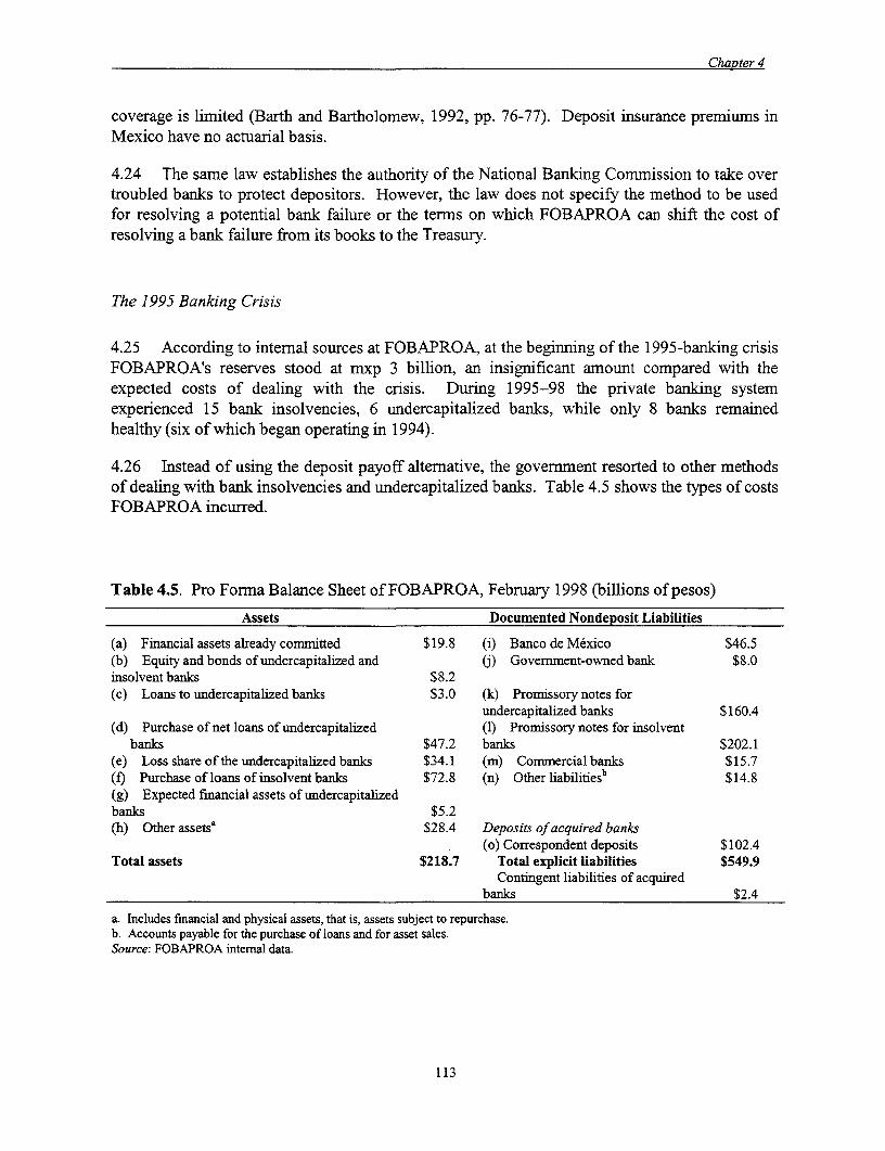
Chapter 4
coverage is limited (Barth and Bartholomew, 1992, pp. 76-77). Deposit insurance premiums inMexico have no actuarial basis.
4.24 The same law establishes the authority of the National Banking Commission to take overtroubled banks to protect depositors. However, the law does not specify the method to be usedfor resolving a potential bank failure or the terms on which FOBAPROA can shift the cost ofresolving a bank failure from its books to the Treasury.
The 1995 Banking Crisis
4.25 According to internal sources at FOBAPROA, at the beginning of the 1995-banking crisisFOBAPROA's reserves stood at mxp 3 billion, an insignificant amount compared with theexpected costs of dealing with the crisis. During 1995-98 the private banking systemexperienced 15 bank insolvencies, 6 undercapitalized banks, while only 8 banks remainedhealthy (six of which began operating in 1994).
4.26 Instead of using the deposit payoff alternative, the government resorted to other methodsof dealing with bank insolvencies and undercapitalized banks. Table 4.5 shows the types of costsFOBAPROA incurred.
Table 4.5. Pro Forma Balance Sheet of FOBAPROA, February 1998 (billions of pesos)
Assets Documented Nondeposit Liabilities
(a) Financial assets already conmiitted $19.8 (i) Banco de Mexico $46.5(b) Equity and bonds of undercapitalized and (j) Govermment-owned bank $8.0insolvent banks $8.2(c) Loans to undercapitalized banks $3.0 (k) Promissory notes for
undercapitalized banks $160.4(d) Purchase of net loans of undercapitalized (1) Promissory notes for insolvent
banks $47.2 banks $202.1(e) Loss share of the undercapitalized banks $34.1 (m) Commercial banks $15.7(f) Purchase of loans of insolvent banks $72.8 (n) Other liabilities" $14.8(g) Expected financial assets of undercapitalizedbanks $5.2(h) Other assetsa $28.4 Deposits of acquired banks
(o) Correspondent deposits $102.4Total assets $218.7 Total explicit liabilities $549.9
Contingent liabilities of acquiredbanks $2.4
a. Includes financial and physical assets, that is, assets subject to repurchase.b. Accounts payable for the purchase of loans and for asset sales.Source: FOBAPROA intemal data.
113

Chapter 4
4.27 The authorities employed two basic measures to deal with bank insolvency: (a) directassistance, which consisted mainly of direct loans or cash infusions from FOBAPROA followedby the Trust's assumption of an equity position in the bank; and (b) financial assistance forpurchase and assumption transactions. In the latter case the insurer solicited bids for the failinginstitution as a going concern. The winning institution would take the good loans and assumedthe liabilities of the failed bank while FOBAPROA acquired any unwanted assets (table 4.4, itemf). In return for capital from the new owners, FOBAPROA issued promissory notes to buyerswith variable maturities of up to ten years (table 4.5, item 1) committing to make a stream offuture payments. According to FOBAPROA officials, in 1999 fiscal resources will be used tofinance this liability.
4.28 A different scheme was developed for undercapitalized banks. Because the quality ofsome assets was difficult to assess or to document, the government decided to acquire someportion of the assets in return for new capital investment from the current owners (table 4.5, itemd). The government assistance took the form of promissory notes with maturity of ten years(table 4.5, item k). The acquisition process required banks to share the possible future losseswith FOBAPROA (table 4.5, item e). The banks have to absorb between 25 to 30 percent of thedifference between the book value of the promissory notes and the actual loan recovery, a rangeFOBAPROA officials determined following negotiations with the banks. In this case, the streamof future payments that FOBAPROA is obligated to pay is contingent on the future performanceof the assets acquired.
4.29 During 1996-98 the government used fiscal resources to motivate various classes ofborrowers to restructure their debts with the banks (table 4.5, item m). In December 1998Congress approved additional fiscal resources to continue with this type of program. The effectof this new measure has not yet been included in the pro forma balance sheet. FOBAPROA hasborrowed from the central bank and from government-owned banks (table 4.5, items i, j, and o)to provide loans and cash infusions to troubled banks.
Expected Fiscal Costs of Resolution of the Crisis
4.30 According to FOBAPROA officials, the 1999 budget includes cash outlays of mxp 18billion for interest payments, or 2.2 percent of total budgeted government expenditure forcontractual obligations.
4.31 The difference of all explicit liabilities and assets shown in table 4.5 represents thenegative net worth (equivalent to net debt) or a present value estimate of the total fiscalassistance provided under FOBAPROA. As of February 1998, this amounted to mxp 331.2billion (mxp 549.9 billion minus 218.7 billion, see table 4.5), or approximately 35 percent of thetotal assets of the troubled banks (at the end of 1994) that remained in the system in 1998.6
4.32 The main assumptions underlying the estimates shown in table 4.5 are a 30 percentrecovery rate of troubled loans and an expected cost of resolving the bank failures of Promex,
6 In contrast, in the 1980s the U.S. Federal Deposit Insurance Corporation averaged losses of approximnately 26percent of the assets of insolvent banks (Brumbaugh and Litan 1992, p. 134).
114
Chapter 4
Atlantico, and Bancrecer of approximately mxp 100 billion. These assumptions are perhapsoptimistic for two reasons. First, the rescue of these three banks has been delayed for more thana year and delays can be expensive (IPAB's June 1999 estimate of the rescue of these three banksis now up to mxp 156.5 billion). Second, the recent increase in real interest rates combined witheconomic and political events will negatively affect FOBAPROA's rate of asset recovery.7 Notconsidered is the possibility that higher real interest rates will reduce the future rate of growth ofthe economy, and consequently the rate of growth of demand deposits and FOBAPROA'sinsurance premiums. It is further assumed that interest rate shocks will not affect the loanrecovery rate of current loans.
4.33 Understanding how the real interest rate shocks will affect FOBAPROA's pro formabalance sheet is important.8 On the asset side we assume that the shock will last almost twoyears and that the elasticity of the loan recovery of FOBAPROA with respect to the real interestrate is unitary. For comparison, Chirinko and Guill (1992, p. 238) estimate the equivalentelasticity for the United States to be around 0.8. Therefore, assuming a real interest rate increasefor 1999 of 20 percent, mxp 47.2 billion in assets from the purchase of the net loans ofundercapitalized banks (table 4.5, item d), and mxp 72.8 billion in assets from the purchase ofthe net loans of insolvent banks (table 4.4, item f), the decline in the value of FOBAPROA'sassets equals (mxp 47.2 + mxp 72.8) x 0.20 = mxp 24.0 billion.
4.34 On the liability side, the recent increase in the real interest rate will not affect the presentvalue cost of financing, because as interest rates on FOBAPROA borrowing change, so will therate at which future outlays are discounted.
4.35 In October 1998, Congress hired Canadian consultant Michael Mackey to audit thebanking operations under FOBAPROA. The audit gave an estimate of a total fiscal cost of mxp633.3 billion and signaled several doubtful transactions according to Mexican banking laws, thelatter amounting to mxp 72 billion.9 The results of this report were used to provide newestimates of the overall cost of the financial rescue. The official estimates through June 1999 areshown in table 4.6.
7 At September, 1999 IPAB's estimation of the rate of recovery of assets was of around 20 percent only.8 Since January 1996 real interest rates have experienced a downward trend. The fitted values of a regression on
January 1996 and August 1998 were 31.1 and 13.8 percent respectively. In September 1998 the actual real interestrate rose to 37.7 percent and remained above 29 percent during the last quarter of 1998. In our example we assumea conservative 20 percent increase in the real interest rate.
9 Whether this transaction becomes public debt is still under a case by case review by the regulatory authorities.
115

Chapter 4
Table 4.6 Estimate of the Overall Cost of the Financial Rescue, June 1999.
Billion ofpesos % of GDPDebtors Aid Programs 174.3 3.9Cost of banking intervention 579 12.8and clean upPurchase of non performing 101.8 2.2assetsToll Roads Program 18 0.4Total 873.1 19.3
Source: IPAB
4.36 Of this 19.3 percent, 3.1 percent as already been spent, leaving a government-acknowledged liability of 16.2 percent of GDP.
4.37 Table 4.7 presents the executed fiscal resources on financial rescue programs, illustratingthat a significant, albeit insufficient, share of fiscal resources have already been channeled toFOBAPROA.
Table 4.7 Executed Fiscal Cost on Programs of Financial and Debtors Rescue (billions of pesos)
Year Current Value Description(billion of pesos)
1995 15 Fiscal surplus used to cover the cost of ADE and other programs
1996 20.5 20 billion for FOBAPROA, the rest corresponds to other programs
1997 39.78 Budget resources used in FOBAPROA (72.8 percent), DevelopmentBanks (24.9 percent) and FOPYME, FINAPE and Debtors of HouseCredits (2 percent)
1998 10.11 Debtors aid (2 billions), Financial Rescue of Nafin, Banrural and others(6.1 billions), FOBAPROA (2 billions)
1999* 25.14 Financial Rescue Programs. Debtors and Conmmercial Bank Programs(88.3 percent), Development Bank Programs (11.7 percent)
Total 110.53* predicted valueSource: SHCP
4.38 Mexico's experience shows that insolvent institutions can not be expeditiously liquidatedor merged with stronger partners. The authorities have engaged in capital forbearance, that is,they have been lenient in solving shortages of private ownership capital at undercapitalizedinstitutions. Kane and Yu (1994) provide empirical evidence that capital forbearance proved tobe a costly strategy for the U.S. thrift industry, resulting from distortionary management and risktaking incentives, and because surviving thrifts had to squeeze their profit margins to meettightened capital requirements.
116

Chapter 4
4.39 Although the cause is not yet known, the expected cost of dealing with Promex,Atlantico, and Bancrecer has already increased by 12 percent from February 199810 to September1998.1" Thus, assuming a similar trajectory, we assume an increase of mxp 10.0 billion in theexpected resolution cost for the three banks. At the present time deciding in terms of equation(5) if this expected loss should be part of the adjusted primary surplus or of the adjusted financialdeficit is not possible.
4.40 As a result of the interest rate shock and delayed bank rescue, FOBAPROA's negative networth will increase by mxp 34 billion (mxp 24 billion plus mxp 10 billion). The decompositionof these new expected losses in terms of equation (5) is mxp 10 billion in the primary surplus andthe rest in a reduction in the rate of return of the assets. Therefore, based on our assumptions, theadjusted fiscal deficit is almost 0.7 percent of GDP higher than the unadjusted fiscal deficit of1.25 percent used in the 1999 budget.
4.41 In order to compare the magnitude of the Mexican banking crisis with the internationalexperience, table 4.8 presents the cost of other banking crises as a percentage of GDP. Here wecan see that the Mexican crisis is among one of the largest crises in the recent history. Figure 4.1presents the potential cost of future banking crisis for several countries as a percent of GDP.
t° The February 1998 estimate was mxp 97.9 billion (see table 4.5, item 1)"As of June 1999 this cost had increased by 60 percent with respect to the February 1998 estimate.
117

Chapter 4
Table 4.8. Estimate of Total Losses of Resolving Major Bank Insolvency
Country % of GDP (*2 Description of the costsArgentina (1980-82) 55.3Chile (1981-83) 41.2 Government assistanceUruguay (1981-84) 31.2 Recapitalizing banks and subsidized credit operationsIsrael (1977-83) 30.0Mexico (1995-99) 19.3Venezuela (1994-95) 18.0Senegal (1988-91) 17.0Spain (1977-85) 16.8 Estimated losses of banksMauritania (1984-93) 15.0 Cost of rehabilitationBulgaria (1990s) 14.0 Banking sector lossesHungary (1991-95) 10.0 Overall resolution costTanzania (1987; 1995) 10.0Brazil (1994/1995) 7.0 Negative net worth of selected state and federal banksSweden (1991) 6.4 Cost of recapitalizationGhana (1982-89) 6.0 Restructuring costsPoland (1990s) 5.7 Recapitalization costColombia (1982-87) 5.0Malaysia (1985-88) 4.7Norway (1987-89) 4.0 Recapitalization costUnited States (1984-91) 3.2 Cost of savings and loan clean upPhilippines (1981-87) 3.0 Central Bank assistanceGuinea (1985) 3.0 Repayment of depositsTurkey (1982-85) 2.5 RescueSource: Caprio. and Klingebiel (1996), Dziobek and Pazarbasioglu (1997); IPAB for Mexico.
118

Chapter 4
Figure 4.1 Contingent Liabilities Related to the Banking Sector (percent of GDP).
0 20 40 60 80 100 120
Korea Thailand-I| M alays ia
'China, _____ _______ Japan
I Czech RepublicEgypt
_ = : = Slovak RepublicI Lebanon
IndonesiaHong Kong
TaiwanIsrael
KuwaitSingapore
AustriaNew Zealand
Greece'. Ireland U * Lower bound (% of GDP)--I Netherlinds
I SwitzerlandPortugal
:SpainBrLazil 0 Difference between upper
IndaaNorway and lower bound (% of
South Africa GDP) Turkey __ rGermany
United KingdomUnited States
ChileColomrbia
Rom aniaAustraliaCanada
ItalyM exico
Russ;iaFrance
HungaryPolarid
VerlezuelaBelgium
DenmarkArgentina
Sw eden:__ _ _ _ _ _ _ __ _ _ _ _ _ ___ _ _ _ _ _ _
Source: Standard & Poor's, Sovereigns Ratings Service. May 1999
119

Chanter 4
Government Credit Assistance Programs
4.42 Government-owned banks provide loan guarantees and direct loans for a variety of policyobjectives. Table 4.9 presents outstanding loans by program area and institution. The totalamount represents 27 percent of total outstanding peso-denominated loans of the banking systemin 1997. For comparison, a recent estimate for 1995 asserts that total federal and federallyassisted borrowing in the US represents 49.6 percent of the total net borrowing in credit marketsby domestic non financial sectors (Cavanaugh 1996).
Table 4.9 Government Loans by Major Program Area, Fiscal 1997 (billions of pesos)
Institution Program area Outstanding loansDirect loans aNafinsa Small and medium businesses 12.2
Government entities 37.3Financial intermediaries 9.0Other credits 1.8
Bancomext Export activities 14.2Government entities 5.4Financial interTmediaries 27.7
Banobras State and municipal infrastructureb 43.4Banrural Agriculture and agro-industry 10.9Banejercito Armny 1.5Fina Sugar industry 11.0Fovic Financial intermediaries (housing) 30.4Firac Financial intermediaries (agro-industry) 19.4Fidecc Wholesale and retail trade 8.1Total 232.3Financial and loan guaranteesdNafinsa 7.3Bancomext 10.9Banobras 5.3Fira 3.4Fovi 11.6Total 38.5a. Excluding loans granted as financial agent of the federal government.b. Mxp 12.5 billion represents loan restructuring in UDI's for states and municipalities.c. Although legally not a development bank, for our purposes it works similarly to a credit agency. The outstanding loans do not
include the asset item by the namne of refinancing of interest.d. Off-balance sheet information.Source: Banks annual reports and CNBV statistical bulletins.
4.43 The loan guarantees are privately held loans, mainly to banks as opposed to firms andindividuals. In the event of default, the government-owned bank guarantees to pay all or some ofthe principal and interest. The financial guarantees (standby letter of credit, note issuancefacilities, and so on) are mainly activities that generate income and/or expenses without thecreation of or holding of an underlying asset or liability.
4.44 Some of the direct loans, for example, the credits to agriculture and housing, involve adegree of subsidy. However, until 1998 the government provided explicit fiscal transfers in the
120

Chapter 4
budget for institutions responsible for providing interest rate subsidies. It discontinued thispractice in the 1999 budget.
Characteristics of Direct Loans and Loan Guarantees'2
4.45 At this point the development banks do not share a common accounting system fortracking loan defaults. In the case of direct loans, some of them are often rescheduled throughtrust funds to delay the appearance of a non-performing loan. With respect to loan guarantees, incase of default the burden of the cost sometimes does not appear in the records of the originatingbank. Therefore, analyzing the situation of each institution in detail is important.
4.46 FOVI is a housing finance liquidity facility administered by the Banco de Mexico. Itsmain objective is to promote and provide affordable mortgage financing to low-incomehouseholds through commercial banks and SOFOLES (special purpose financial companies thatoriginate mortgage loans). FOVI financing is only provided to low-income households that earn2 to 8 monthly minimum wages, about USD$2,000 to USD$8,000 per annum. FOVI's principalmortgage product is targeted for individual new home purchases. It also provides constructionloan mortgages to housing developers to aid in the construction of new homes (up to 65 percentof property sales price). These loans are repaid when individual mortgage loans are originated infavor of the new home owners. FOVI funds projects that are approved though a transparentbidding process where developers bid a certain premium (0.1 percent minimum) on the amountto be borrowed to obtain credit rights. Since 1998, FOVI has also administered the PROSAVIProgram, a small SHCP home mortgage program, targeted to very low-income households. FOVIcurrently obtains its funding from an SHCP loan, from the World Bank, and through its ownequity. FOVI also received preferential tax treatment from SHCP due to the institution'sdevelopment financing nature.
4.47 As a liquidity provider, FOVI's exposure to credit risk is limited to its commercial banksand the SOFOLES only, not to the homeowners. Since March 1994, FOVI has provided a 50percent guarantee to the originating institutions, but this affects only a very small part of FOVI'sbalance sheet. For the PROSAVI loans, FOVI bears no risks. Even though these loans are shownas assets on the FOVI balance sheet, SHCP guarantees 100 percent. It is important to identify thedifference between FOVI's portfolio and the home mortgage portfolio funded by FOVI. Theformer essentially has no defaults or past dues because FOVI, as a trust fund of Banco deMexico, has first call on the banks' and SOFOLES' balances at the central bank; the latter, whichis the credit risk of the participating banks and SOFOLES, does have defaults and past dues.After the financial crisis started in late 1994, in the banks, the "cartera vencida" (default loans)has been on the order of 25 percent, and in the case of SOFOLES, it has been about 3 percent.The difference is due to originating and servicing skills of these two types of institutions.However, this "cartera vencida" is not a contingent liability of FOVI nor of the govermnent.
12 See page ii for directory of acronyms.
121
Chapter 4
4.48 FOVI offers inflation adjusted loans through a double-index mortgage (DIM) instrument.The FOVI DIM is quite different from other DIMs in the Mexico market. In the FOVI DIM,monthly payments are indexed to monthly minimum wages and the mortgage balance is indexedto inflation (CETES or UDIs). The maximum repayment term is fixed but the maturity of theloan oscillates within a band that allows the loan to be paid-off before the maximum repaymentterm. At the same time, FOVI limits the payment factor to a maximum of 25 percent ofhousehold income. The borrowers are not shielded from interest changes, hence under the mostsevere financial crisis, negative amortization can accumulate, creating a contingent liability forFOVI when end-of-term balances build up. FOVI writes these balances off after 30 years of loanlife.
4.49 For years FOVI received subsidized funding from the Government and providedsubsidized funding, plus a spread, to the first tier lending institutions. Therefore, 'FOVI's retumshave been much lower compared to the rest of the market but caused no particular solvencyproblems to the institution. However, this situation is about to change and can cause anasset/liability mismatch when FOVI no longer funds its operations from subsidized resources andhas to move to market funding at market rates. The Government has paid special attention toFOVI's weaknesses and its own exposures. It began to discuss a major restructuring program forFOVI in 1995, and is now implementing it with Bank support. The guiding principles of therestructuring program will include the introduction of a market-based mortgage instrument,improvement of credit quality, emphasis on private market securitization rather than providingGovernment guarantees, and strengthening all participating institutions in the sector.
4.50 In order to implement the FOVI restructuring project, FOVI will move to market-ratemortgage instruments, and on limited scale, combine these with upfront subsidies; introduce aneligibility program for participating institutions; introduce a modified DIM, including a fee forthe end-of-term (i.e., thirty years) exposure; work with a private sector strategic partner todevelop an improved insurance product, with the intention of eventually privatizing this line ofbusiness (50 percent guarantee); work with private, issuers to develop a secondary mortgagemarket such that securitization will eventually become a major source of revenue (firstsecuritization will take place in the year 2000); become an international rated, US GAAPinstitution; bring a second tier of management, including a COO, a CFO and a CIO to implementthe changes proposed; and acquire additional capital.
4.51 INFONAVIT is the largest pension fund, and at the same time, the largest housing fund inMexico. It covers employees in the private sector assigned to the social security system. Createdin 1972 with federal government capital and financed with employers' contributions (5 percent ofworkers'. salary), INFONAVIT provides resources for housing investment and mortgage credit.The federal government, employers, and the employees form the "Board of Directors" of theinstitution.
4.52 Prior to 1992, all contributions were accumulated in a single account, with no distinctionamong workers. The fund did not report the individual savings balance to the worker, andborrowers did not receive a sumnmary report of their credit balance. The companies selected byINFONAVIT to build houses had a captive market in the fund's accredited members, who couldnot choose housing alternatives other than those provided by the institute. In 1992 the National
122

Chapter 4
Housing Fund was linked to the social security system and reforms were implemented inINFONAVIT's operational guidelines. Some examples of these new policies include the reportof saving and debit balances to the workers,13 the use of auctions to assign credits forconstruction, and the possibility of acquiring a house in the open market. Nevertheless, problemsremain. For example, the credit line to acquire a house in the open market was subject to a highlydiscretionary process. In addition, the credit assignment mechanisms generated undesiredoutcomes in terms of the quality of the housing and the population benefiting from thosecredits.'4
4.53 In 1997 INFONAVIT was reformed again to comply with the new, fully-funded socialsecurity system implemented by IMSS. The main reforms included the creation of individual'spension fund housing sub-accounts (as components of the overall social security accounts), theseparation of INFONAVIT resources from these sub-accounts, and several policies intended toreduce administrative costs. The new scheme allows employees to deposit voluntary savings intheir housing sub-account with a monitored and individualized system.
4.54 Despite these reforms, mortgage loan defaults represent a severe problem that threatensthe solvency of the fund. Given the poor disclosure on INFONAVIT's liabilities, it is difficult toquantify the underlying contingent liabilities. From a legal standpoint the federal governmentdoes not have an obligation (because the employers/employees finance the system), yet there isan implicit obligation. Public information on the financial status of the institution is necessary toassess the contingent liabilities of INFONAVIT.
4.55 FIRA offers loans to primary producers and agro-industries through participating privatebanks and the government owned BANRUTRAL. FIRA also offers a loan guarantee programwhereby participating banks can obtain guarantees up to 90 percent of loans by qualifiedcustomers (primary producers and agro-industry). FIRA charges a loan insurance fee ofapproximately 3 percent of the guaranteed loan value. Whether this is an actuarially sound fee isunclear given the large variation in loan defaults this program has experienced (some 1 percent inthe 1980s and 10 percent in the 1990s). Apparently FLRA does make some provision for loanlosses, but it does not show up on the balance sheet. It is possible some of the losses resultingfrom the financial crisis of 1995 actually appear in the books of BANRURAL and FOBAPROA.
4.56 FIRA receives the same preferential tax treatment as FOVI, and has a long-term loan fromthe Central Bank worth mxp 46.1 billion; however, the government has waived repayments forthe past five years. Therefore, because most of FIRA's lending is short term, it has built up asignificant liquidity reserve that has doubled its portfolio of outstanding loans.
13 Nevertheless, the pay-as-you-go system was still dominant.4 First, one outcome was the financing of low quality homes. Second, the points system used to assign mortgage
loans punished young households and growing cities.
123

Chapter 4
4.57 The asset side of the balance sheet shows an item referred to as "lending to refinanceinterest rate payments." This exists because FIRA charges a real interest rate and has acquiredpast due loans from other institutions.1 5
4.58 FIRA has to start repaying the central bank at the end of 1999. This is unlikely to presenta problem initially given FIRA's high liquidity reserves, but the long-term outlook is uncertain.No budgetary fiscal transfers are indicated for FIRA in 1999, and loan recovery will depend onthe economic performance of the agriculture sector. Thus, given current circumstances, FIRA'slending program may not be sustainable in the long run.
4.59 FIDEC offers direct loans for the wholesale and retail trade to participating banks. Loansfrom the central bank totaled mxp 12.8 billion at the end of 1997. However, FIDEC's situation isdifferent from FIRA's because the inflationary component on the asset side is almost null.Therefore, the preferential tax treatment that it receives, combined with its long-term lendingprivileges at the central bank, mean that FIDEC is better positioned to meet its obligations.
4.60 FIDEC has no reserves for loan losses by design. This means that the private banks haveabsorbed any loan defaults prior to 1994, because FIDEC receives loan repayments automaticallyfrom the participating banks. Losses incurred after 1994 would appear on FOBAPROA's booksafter the participating bank has paid FIDEC. As in the case of FIRA, assessing the amount ofloan defaults as a result of this program is difficult.
4.61 NAFINSA provides various types of credits to firms in the manufacturing sector, mainlythrough the banking system. The loan guarantee program for small and medium firms is new andsmall. NAFINSA's financial guarantees cover many different types of off-balance commitments,and as of December 1997 amnounted to mxp 7.4 billion. A clear picture of their riskcharacteristics is hard to derive because the information is confidential at this point.
4.62 Because of the 1995 crisis, as of December 1997 NAFINSA decided to shift mxp 28.9billion from bad loans to private borrowers to a government trust, FIDELIQ. The reality is thatthis amount is already a government liability, as the alternative would have been dealing with aninsolvent bank. As a result of this accounting treatment, the risk of this loan is zero andNAFINSA can comply with the capital adequacy requirement. The governnent has delayedinterest rate payments to NAFINSA.
4.63 BANOBRAS provides direct loans for urban infrastructure, such as water supplyfacilities, sewer systems, highways, housing, mass transit, roads, and bridges. Intergovernmentaltransfers to states and municipalities guarantee most of these loans. Prior to 1995 the bank alsoprovided direct loans and loan guarantees for the road construction by the private sector. Thevalue of the direct loans and loan guarantees for the construction of roads by the private sector atthe end of 1997 was mxp 7.4 billion, 17 percent of the bank's total outstanding loans (excludingloans provided as a financial agent of the government). BANOBRAS is one of the fewdevelopment banks that do not receive direct subsidies or budget transfers from the government.
IS These accounting and lending practices are a response to the distortion introduced by inflation. The nominalinterest rate includes principal amortization, so the burden of the loan for the borrower is artificially higher in theinitial periods. The value of the lending for refinancing interest rate payments was mxp 12.1 billion in 1996.
124

Chapter 4
Funding comes from the World Bank, the IDB, Eximbanks and the emission of bonds in thenational capital markets.
4.64 After the 1995 crisis the government decided to create a trust named FARAC. Throughthis legal structure the government became the owner of the roads that were concessions to theprivate, and therefore has acquired a liability with BANOBRAS. Also as a result of the 1995crisis the government decided to restructure loans to states and municipalities by means ofanother trust administered by BANOBRAS. The renegotiated loan amounts to mxp 9.3 billion.The fiscal risk of this program warrants further investigation.
4.65 BANCOMEXT provides a loan guarantees to assist exporters. A participating bank canobtain a guarantee for up to 70 percent of the loan to a qualified firm oriented toward exportmarkets. The loan insurance fee is between 0.5 percent and 3 percent of the principal, anddepends on the amount of the guarantee and the performance of the participating bank.According to the 1997 annual report, the bank did not incur any losses on operations in which itacted as guarantor. This is quite unusual for small and medium firms. Nevertheless, the bank isin good financial condition, so future problems are not anticipated.
4.66 BANRURAL provides subsidized credit to small farmers and the agro-industry sector.The reality is that the bank is insolvent. According to official statistics, as of June 1998 morethan 50 percent of total outstanding loans were in arrears, amounting to more than seven timesthe value of the stockholders' equity. The government is attempting to recapitalize the bank at anestimated cost of more mxp 9.0 billion, necessary in order to meet capital adequacy requirements(assuming no recovery of past due loans).
4.67 FINA is a loan program designed to assist the sugar industry. According to officialstatistics, the bank's capital adequacy ratio was below the minimum level of 10 percent. during1997 and part of 1998, which indicates that it is undercapitalized. However, in reporting itsassets the bank has not reported past due loans, making determination of its outlook unclear.
4.68 In March 2000 the government will issue a new regulatory framework for developmentbanks compatible with that of commercial banks. Modifications will include improvements incredit monitoring, risk management, and lending control through the use of default records of theclients, as well as new capital adequacy rules. This reform seeks to put an end to the duediligence problems that permeate development banks, as well as to standardize capital normsacross banks. The urgency of the reform made clear by the profitability problems facingdevelopment banks. According to the CNBV, as of September 1999 these banks accumulatedaggregate losses approaching 1.7 billion pesos (85 percent of these losses are FINA andBANOBRAS16). The strength of this initial reform will depend on the scope and enforcement ofthe new rules.
16 Authorities claim that these negative numbers are the result of the stricter banking rules faced by developmentbanks, as well as of the crisis in sugar production (in the case of FINA). Nevertheless, it is irnportant to rememberthat in the past bad loans from development banks have been assumed by funds like FARAC and FIDELIQ.
125
Chapter 4
Expected Fiscal Cost of Government Credit Programs and the Budget
4.69 The lack of accessible data on the life cycle of direct loans and loan guarantees makes itdifficult to predict default risk. Under these circumstances, any estimate of the government'sliability will be subject to criticism.
4.70 With respect to FIDEC, FOVI and FIRA none has a negative net worth, in large partbecause of the way these programs have been designed. However, FIRA's and FOVI's programsmay pose significant risks for the future. Estimating the magnitude of the risk is difficult, but forthe time being our purpose is merely to draw the attention to the problem. Under the worst-casescenario, the Central Bank will continue its support to FIRA and FOVI. The expenses incurredwill show up as a reduction in profits to the Treasury in the event that the agencies postponerepayment of their loans. In the case of NAFINSA, the government has not defined howNAFINSA will cover its explicit liabilities. In determining the fiscal risk exposure forNAFINSA, we assume that the government does not want to maintain NAFINSA under a capitalforbearance policy and we further assume:
- Average annual interest rate for 1998 and 1999 30 percent3 Loan recovery rate before the real interest rate shock of
September 1998 30 percent* Elasticity of the loan recovery rate with respect to the real
interest rate 1* Loan recovery rate assuming an increase of 20 percent in
the real interest rate after the shock of September 1998 24 percent- NAFINSA's asset with FIDELIQ as of December 1997 mxp 28.9 billion.
Under this scenario we can make the following calculations:
4.71 The difference between FIDELIQ's liabilities for NAFINSA (mxp 28.9 billion) and itsassets (mxp 28.9 billion x .30) equaled mxp 20.2 billion as of December 1997. The samedifference equaled mxp 28.9 billion [(mxp 28.9 x 1.30) - (0.30 x mxp 28.9 billion)] in December1998, and will amount to mxp 42.0 billion [(mxp 37.6 billion x 1.30) - (0.24 x mxp 28.9 billion)]in December 1999.
4.72 Therefore the estimated change in the net worth of NAFINSA with FIDELIQ from 1998to 1999 amounts to rnxp 13.1 billion (mxp 42.0 billion - mxp 28.9 billion). Using equation (5),we need to adjust the fiscal balance for 1999 by some 0.25 percent of GDP. Finally, the pendingcapitalization of BANRURAL of approximately mxp 10.0 billion is still on hold and how it willbe financed is unknown. At minimum, the estimated impact would be an increase in the fiscaldeficit by another 0.2 percent of GDP in 1999.
126
Chapter 4
Liabilities Related to Social Security Programs
4.73 In December 1995 the government publicly acknowledged the financial unsustainabilityof the private employment retirement, disability, and medical insurance schemes provided by theIMSS. It introduced reforms that resulted in the elimination of cross-subsidies between medicaland retirement expenses and the substitution of the pay-as-you-go system with a fully fundedsystem with individual accounts and a minimum pension guarantee. The government has not
addressed the financial sustainability of the federal civil service retirement system provided by
the ISSSTE publicly, although some actuarial data are available. No information is availableabout military pensions.
The Financial Condition of IMSS
4.74 The pension reform of 1995 meant that the unfunded liability of the retirement systembecame a government liability. Several estimates of the size of the unfunded liability at the end
of 1994 are available. Sales, Solis and Villag6mez, (1997) claim that the actuarial imbalance of
the pension system was at least 80 percent of GDP. Cerda and Grandolini (1998) mention an
actuarial imbalance of 141 percent of GDP based on IMSS estimates. These numbers seem to bea so-called "open group estimate" that includes the contributions of future participants in thelabor market.1 7 That is why the estimates often cover a longer period than the 70-year standard
long-term actuarial projection period.
4.75 If we use closed group IMSS estimates of the unfunded actuarial liability the deficit ismxp 203.4 billion, or 16 percent GDP, as shown in Table 4.10 (using a 40-year actuarialprojection period). This estimate does not include future generations, uses a real interest rate of3.5 percent, and can be considered optimistic. Although the estimates are not strictly comparable
because of the different assumptions, the structural reform of the retirement system has resulted
in a significant fiscal impact.
Table 4.10 IMSS Retirement System Actuarial Deficit, December of 1994 (billions of pesos)
Category ValuePresent value of projected benefit payments 613.9Present value of future contributions 406.1Current assets 4.4Excess of liabilities over assets 203.4Source: IMSS (1994).
4.76 Table 4.11 presents the government's net liability for the closed group, when futureparticipants are no longer a government liability as of mid-1997. Note this figure approaches 50percent of GDP.
7 The terminology has been adopted from Bohn (1992) and Boskin, Robinson and Huber, (1989). Under a closedgroup approach the expected future taxes and benefits of those currently in the labor market are calculated. In theopen group approach the expected present value of taxes and benefits of individuals who are not yet in the laborforce are counted.
127

Chapter 4
Table 4.11 Government Net Liability as a Result of the 1995 Pension Reform(billions of 1997 pesos)
Assets LiabilitiesFinancial assets (IMSS transfers)a 5.2 Old age benefitsb 1274.9
Death and disability benefits 453.0Excess of liabilities over assets 1722.7
a. Actuarial reserves transferred from the IMSS to the government.b. Approximate present value at a discount rate of 11.5 percent of fiuture flows.Source: Gonzalez (figure 4, 1997); IMSS data.
4.77 The next step is to determine how the accrual estimates of the new social securityobligations should be reflected in the primary balance. We have to use the right-hand side termof equation (5) because actuarial values for 1998 are not available. The correct measure is notcurrent payments to beneficiaries, but new pension obligations. For 1999 the budgetedexpenditure on pensions is 0.7 of GDP. To provide an estimate of the future cost we use 0.85percent of GDP for old age benefits (the average value of Gonzalez 1997, figure 4). The latterestimate does not include the expected future cost of death and disability benefits. Using internalIPSS estimates another 0.05 percent of GDP should be added. Adjusting for these twoadditional factors implies an adjustment to the primary balance of 0.2 percent of GDP (0.85percent + 0.05 percent - 0.7 percent).
4.78 The government has promised to subsidize the hospital insurance program, therebymaking it an explicit liability. The World Bank Mexico Health System Reform Project, IMSS,(May 18, 1998) estimated that the average annual fiscal cost of the health reforms will amount to0.5 percent of GDP for the next ten years. In 1997 and 1998 fiscal transfers to the IPSS wereapproximately 0.4 percent of GDP, the same as budgeted expenditure for 1999. Therefore, theaccrual primary balance should be at least 0.1 percent of GDP more than the current outlay.
The Financial Condition of the ISSSTE
4.79 The government employee pension fund is a liability for the government. In this case anestimate of the open group is important because the pay-as-you-go system is still in place. In1995 the ISSSTE had an estimated actuarial deficit between mxp 715.0 billion to mxp 1,303.0billion (depending on the assumptions used). Thus this obligation is substantial, amounting tosome 28 to 52 percent of GDP in 1996 (see ISSSTE, 1995).
4.80 Current cash outlays do not reflect the future fiscal cost to the government. We canestimate future costs using the same approach as that used for the IMSS. For 1999 the budgetedexpenditure on ISSSTE pensions is 0.3 percent of GDP, of which approximately half will befinanced by fiscal resources. Assuming an actuarial deficit of around 40 percent of GDP(average value of the numbers provided earlier) and a structural reform similar to the IMSS case,
128

Chapter 4
the additional adjustment in the fiscal deficit for the ISSSTE would be some 0.5 percent of GDPin the near future.'8
Expected Fiscal Costs of Social Security Programs and the Budget
4.81 Given the IMSS pension reforms and the significant federal employee pension funds, thefiscal outlook is not promising. In terms of equation (5) we have obtained an adjusted fiscaldeficit of 0.8 percent of GDP, all of which should be included in an adjusted primary balance.
Private Provision of Infrastructure and Government Guarantees
4.82 Since the 1990s the private sector has been involved in the provision of power plants andhighways. Although initially no explicit government guarantees were involved this changedbecause of the 1995 financial crisis, when the government had no option but to absorb anydefaults.
Power Plants
4.83 Since the mid-1990s the Federal Electricity Company (CFE) has signed take-or-paycontracts with independent private producers and/or has leveraged lease schemes. In the formercase, the CFE is required to pay in U.S. dollars for a contractually specified minimum quantity ofenergy, even if delivery is not taken. As concerns leasing schemes, if the leasing fees were equalto the users' cost of CFE capital stock, the company's net worth would remain unchanged.According to CFE estimates, the ratio of average revenues to average costs has been 0.7 in recentyears, and the company has not received any fiscal transfers. Under these circumstances, thecompany had no other option but to resort to subcontracting, given the impossibility ofrecovering the cost of capital.
4.84 According to the General Public Debt Law, current liabilities are defined as the currentyear's and the next year's payments. The balance should be classified as a contingent liability.According to CFE managers they have no clear way to put all this on the balance sheet (forexample, should we consider the subcontracting as a contingent liability for the government?)CFE's retail prices are likely to be insufficient to pay the independent producers. In any event,given the presence of highly subsidized prices, the government could pass the bill on toconsumers, a difficult political proposition.
1 If 50 percent of GDP implies a fiscal cost of 0.9 percent (IMSS case), then 40 percent of GDP implies a fiscal costof 0.7 percent. The difference between this number and the actual fiscal cost (around 0.2 percent) results in 0.5percent of GDP.
129

Chapter 4
Highways
4.85 The government did not guarantee a minimum traffic volume in connection with theprivate provision of toll roads, nevertheless, in 1997 the government rescued the private roads.Table 4.12 presents the balance sheet of FARAC, the trust designed to rescue the roadconcessions to the private sector. In present value terms FARAC has a negative net worth ofmxp 14.0 billion. According to Secretaria de Comunicaciones y Transportes (SCT) officials, thebudget for 1999 has no appropriation for paying private concessionaires or BANOBRAS. Thefiscal risk of this rescue depends on the future growth of the economy, therefore it needs to beevaluated annually.
Table 4.12 Pro Forina Balance Sheet of FARAC as of November 1998 (billions of pesos)
Assets LiabilitiesPhysical assetsa 44.0 Banking loansb 30.8
Promissory notesc 27.4Total assets 44.2 Total liabilities 58.2
a. The present value of the net benefits of the roads assumning a real rate of growth of 3 percent in revenues, real discount rate of5.95 percent, and expenses as 25.43 percent of revenues.b. The private banks and BANOBRAS have sent their bad loans to FARAC.c. The government has issued promissory notes to pay the private concessionaires.Source: SCT data; author estimates.
The Fiscal Cost of Government Insurance Programs
4.86 One purpose of this chapter is to provide a preliminary estimate of the government'scontingent liabilities, sumrnarized in table 4.13 below where we have totaled the previousanalyses. Some of these liabilities have become explicit liabilities, such as those related to thedeposit insurance scheme, to several development banks, and to government trusts. Others areimplicit liabilities such as those related to the social security system.
130
Chapter 4
Table 4.13 Contingent Liabilities and Fiscal Deficit Adjustments
Type of Institution Nominal value of net Net liability Adjustment in theContingent Or liability as a percentage deficit as aLiability Trust fund (billions of pesos) of GDP percentage of GDP
Explicit liabilitiesDeposit insurance FOBAPROA 331.2 (February 1998) 10.7 0.7Direct loans andguarantees ofdevelopment banks
NAFINSA 28.9 (December 1997) 0.9 0.25BANRURAL 10.0 (June 1998) 0.3 0.20FARAC 14.0 (December 1998) 0.4
Implicit liabilitiesFunded social IMSSsecurity 1,593.0 (June 1997) 50.0 0.30Unfunded social ISSSTEsecurity 1,009.0 (December 1995) 40.0 0.50
Total 2,986.1 102.3 1.95
Source: Author's calculations.
4.87 The net liability as a percentage of GDP shown in Table 4.13, column 4 should beinterpreted as the expected fiscal cost. However, strictly speaking, the discounted values of eachof the liabilities refer to different time periods. Nevertheless, the total value of 102.3 percent ofGDP provides a crude estimate of the magnitude of the problem.
4.88 Throughout the chapter equation (6) has provided the link between stocks and flows. Intable 4.13, column (5), the point estimates of each liability represent the adjustment in the fiscaldeficit needed to obtain an accrual basis for accounting. According to the preliminary estimates,the accrual deficit is 1.95 percent of GDP higher than the cash flow deficit of 1.25 percentprojected for 1999.
4.89 Although it has been estimated as an important accrual deficit, it should not be addeddirectly to the budgeted fiscal deficit. The latter includes interest payments on contractualobligations, whereas the former covers different sorts of government responsibilities. What isimportant for reporting purposes along with the budgeted fiscal deficit is a yearly evaluation ofthe projected costs of govenmment insurance programs. The value of the liabilities must bereassessed as further information becomes available.
4.90 Since 1998 the Ministry of Finance has made an effort to report what they recognize asthe contingent liabilities of the government. Table 4.14 presents their most recent report.Although this table is not fully comparable with table 4.13, it is not surprising to see the valueincreasing through time.
131

Chap2ter 4
Table 4.14 Contingent Liabilities Recognized by the Federal Government (billions of pesos)
Balance Balance Change from Balance Change fromDec, 1998 Mar, 1999 Dec 1998 Jun, 1999 Dec 1998
FOBAPROAa 425.03 435.17 10.14 451.79 26.76
FARAC 73.63 79.09 5.46 83.32 9.69
Credit Assistance 143.57 153.51 9.94 160.19 16.62
Prograrns b
Development 10.08 11.34 1.26 12.02 1.94Banks
FAMEVAL 4.07 4.33 0.26 4.48 0.41
Others c 5.18 4.72 -0.46 4.66 -0.52
Total d 661.56 688.16 26.60 716.46 54.90a/ Includes only the explicitly guaranteed liabilities by the Federal Government.b/ Includes mainly FIRA, FOVI, FIDEC and FIDELIQ.c/ Includes mainly the Federal Electricity Company, CFE.d/Prelirninary data. It excludes guarantees established in the organic laws of the Development Bank.Source: SHCP
4.91 Public estimation of these liabilities by the government is an important step towardresolution of the problem. However, it must be pointed out that these estimates exclude all sub-national debt, sub-national pensions, some unrecognized FOBAPROA debt, and obligations ofstate-owned enterprises. The problem with these liabilities is that it is difficult to evaluate theirrisk of default in advance with the limited amount of public information available.
Policy Implications
4.92 Developing additional fiscal indicators that describe constraints on government activity isimportant. One such constraint is the estimated mxp 2,986.1 billion in government netcontingent liabilities estimated in this chapter. Assuming a 7 percent annual real interest rate 9this implies an annual cash requirement, in real terms, of nearly rnxp 210.0 billion (4.5 percent ofGDP in 1999) to satisfy the intertemporal budget constraint.
4.93 The government will have to decide how to finance this contingent liability in the future.Some of the options available are implementing tax reforms, changing government programs, orusing available tangible assets (such as electricity or oil). Clearly much work remains to be doneto achieve a successful fiscal adjustment.
4.94 The cost-effectiveness of the development banks' credit programs needs to be addressed.Rather than reducing risk, government guarantees are shifting risk to taxpayers and adding risk tothe economy.
4.95 Budget accounting reform of federal credit programs is needed. Distinguishing clearlybetween the cost of government subsidies and the benefits to subsidized borrowers is important.
19 It is important to note that in the banking section of the chapter, the real interest rate (RIR) used is an ex-ante shortterm rate, while here we refer to an ex-ante long term RIR.
132

Chapter 4
These programs can no longer be treated as simple off-budget programs. Several credit programsare not financially sustainable in the long run under current circumstances.
4.96 The unfunded liability of the ISSSTE is critical, as is the analysis of the military andsubnational pension systems. This analysis should be conducted in conjunction with reform ofthe federal civil service retirement and health insurance systems.
5.90 The Public Debt Law needs to be examined in connection with the topic of contingentliabilities, particularly for the power plants. Several issues are unclear, and budgetary analysis isrequired given the proposed reform of the electricity sector. In addition, adequate incentives forthe provision of private infrastructure need to be designed to avoid the privatization-nationalization cycle.
5.91 The fiscal costs of the bank rescue may have been underestimated, given the structuralbreak in real interest rates in September 1998 and the delay in addressing bank failures.
5.92 SHCP's new quarterly assessment of the contingent liabilities facing the government is animportant step, although a number of areas are omitted from the analysis.
133

Chapter 4
References
Barth, James R. and Philip F. Bartholomew. 1992. "The Thrift Industry Crisis: RevealedWeaknesses in the Federal Deposit Insurance System." in James Barth and R. DanBrumbaugh, Jr. Eds. The Reform of Federal Deposit Insurance: Discipling the Governmentand Protecting the Taxpayer. New York: Harper Collins.
Blejer M. and A. Cheasty. 1991. "The Measurement of Fiscal Deficits: Analytical andMethodological Issues", Journal of Economic Literature, XXIX, (December):1644-1678.
Bohn, Henning. 1992. "Budget Deficits and Goverunent Accounting." Carnegie-RochesterConference Series on Public Policy 37:1-84, North-Holland.
Boskin, Michael, et al. 1987. "The Federal Budget and Federal Insurance Programs" in MichaelBoskin, ed. Modern Developments in Public Finance: Essays in Honor of Arnold Harberger.New York: Basil Blackwell.
Boskin, Michael, M. Robinson and A. Huber. 1989. "Government Saving, Capital Formation,and Wealth in the U.S, 1947-1985." in Robert E. Lipsey and Helen Stone Tice, eds., TheMeasurement of Savings. Investment, and Wealth. Chicago: University of Chicago Press.
Bosworth, Barry P., Andrew S. Carron, and Elisabeth H. Rhyne. 1987. The Economics of FederalCredit Programs. Washington, D.C.: The Brookings Institution.
Brumbaugh, Dan and Robert Litan. 1992. "A Critique of the Financial Institutions Recovery,Reformn and Enforcement Act (FIRREA) of 1989 and the Financial Strength of theCommercial Banks." in Jamnes Barth and R. Dan Brumbaugh, Jr. eds. The Reform of FederalDeposit Insurance: Discipling the Government and Protecting the Taxpayer. New York:Harper Collins.
Cavanaugh, Francis X. 1996. The Truth about the National Debt. Boston: Harvard BusinessSchool Press.
Cerda, Luis and Gloria Grandolini. 1998. "The 1997 Pension Reform in Mexico." World BankPolicy Research Working Paper No. 1933. Finance, Private Sector, and Infrastructure Unit,Latin America and the Caribbean Regional Office, World Bank, Washington, D.C.
Chirinko, Robert S., and Gene D. Guill. 1992. "Aggregate Shocks, Loan Losses, and PortfolioConcentrations: Lessons for Assessing Depositary Institution Risk." in James Barth and R.Dan Brumbaugh, Jr. eds. The Reform of Federal Deposit Insurance: Discipling theGovernment and Protecting the Taxpayer. New York: Harper Collins.
Gonzalez, Eduardo. 1997. "Costos y Equidad de la Reforma al Sistema de Pensiones." Gaceta deEconomia 2 (Spring).
IMSS (Instituto Mexicano del Seguro Social). 1994. "Valor Actuarial del Seguro." Planning Unit,Mexico City
134

Chapter 4
ISSSTE, (1995), Subdirecci6n General de Finanzas, Valuaci6n Actuarial y Financiera al 31 deDiciembre.
Kane, Edward, and Min-Teh Yu. 1994. "How Much Did Capital Forbearance Add to the Tab forthe FSLIC Mess?" NBER Working Paper No. 4701. National Bureau of Economic Research,Cambridge, Massachusetts.
Lewis, Christopher M., and Ashoka Mody. 1997. "The Management of Contingent Liabilities: ARisk Management Framework for National Government." in Timothy Irwin et al., eds.,Dealing with Public Risk in Private Infrastructure. Washington, D.C.: World Bank.
Polackova, Hana. 1999. "Contingent Government Liabilities: A Hidden Fiscal Risk.", Financeand Development, 36-1:46-49.
Polackova, Hana. 1998. "Government Contingent Liabilities: A Hidden Risk to Fiscal Stability."World Bank Policy Research Working Paper No. 1989. Poverty Reduction and EconomicManagement Unit, Europe and Central Asia Regional Office, World Bank, Washington, D.C.
Sales, Carlos, F. Solis and A. Villag6mez. 1997. "La Reforma al Sistema de Pensiones: El CasoMexicano." Gaceta de Economia, (spring).
Solis, Fernando, and Alejandro Villag6mez. 1999. "Fiscal Sustainability in Mexico."Unpublished paper.
Towe, Christopher, M. 1991. "The Budgetary Control and Fiscal Impact of GovernmentContingent Liabilities." International Monetary Fund Staff Papers 38 (1): 109-34.International Monetary Fund, Washington, D.C.
, 1990. "Government Contingent Liabilities and the Measurement of FiscalImpact." International Monetary Fund Working Paper, WP/90/57, June. InternationalMonetary Fund, Washington, D.C.
, 1989. "Optimal Fiscal Policy and Government Provision of ContingentLiabilities: the Example of Government Loan and Deposits Guarantees." InternationalMonetary Fund Working Paper, WP/89/84, October. International Monetary Fund,Washington, D.C.
135

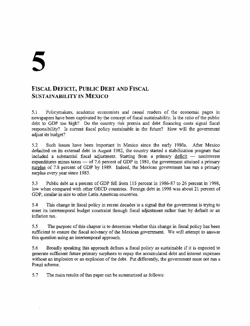
FISCAL DEFICIT, PUBLIC DEBT AND FISCALSUSTAINABILITY IN MEXICO
5.1 Policymakers, academic economists and casual readers of the economic pages innewspapers have been captivated by the concept of fiscal sustainability. Is the ratio of the publicdebt to GDP too high? Do the country risk premia and debt financing costs signal fiscalresponsibility? Is current fiscal policy sustainable in the future? How will the governmentadjust its budget?
5.2 Such issues have been important in Mexico since the early 1980s. After Mexicodefaulted on its external debt in August 1982, the country started a stabilization program thatincluded a substantial fiscal adjustment. Starting from a primary deficit - noninterestexpenditures minus taxes - of 7.6 percent of GDP in 1981, the government attained a primarysurplus of 7.8 percent of GDP by 1989. Indeed, the Mexican government has run a primarysurplus every year since 1983.
5.3 Public debt as a percent of GDP fell from 115 percent in 1986-87 to 26 percent in 1998,low when compared with other OECD countries. Foreign debt in 1998 was about 21 percent ofGDP, similar in size to other Latin American countries.
5.4 This change in fiscal policy in recent decades is a signal that the government is trying tomeet its intertemporal budget constraint through fiscal adjustment rather than by default or aninflation tax.
5.5 The purpose of this chapter is to determine whether this change in fiscal policy has beensufficient to ensure the fiscal solvency of the Mexican government. We will attempt to answerthis question using an intertemporal approach.
5.6 Broadly speaking this approach defines a fiscal policy as sustainable if it is expected togenerate sufficient future primary surpluses to repay the accumulated debt and interest expenseswithout an implosion or an explosion of the debt. Put differently, the government must not run aPonzi scheme.
5.7 The main results of this paper can be summarized as follows:

Chapter 5
5.8 Budgets are affected by oil prices, as total revenues follow the cycle of oil revenues quiteclosely. In response to this vulnerability to oil prices, the stance of fiscal policy has remainedcautious. The latter has been achieved by running consecutive primary (interest exclusive)surpluses since 1983.
5.9 This primary surplus has been obtained primarily by drastic expenditure cuts. As afraction of GDP, non-interest expenditures fell from about 25 percent in the 1980s to 19 percentin the 1990s, a drop of 23 percent. In particular, the major adjustment in the 1990s came fromcapital expenditure. By contrast, non-oil revenue remained roughly constant at about 16.25percent of GDP over this period. The latter in spite of major tax reforms undertaken by Mexicoin the 1980's.
5.10 Mexico's public debt, relative to GDP, fell from 115 percent in 1986-87 to about 26percent in 1998, due to primary surpluses and a debt management strategy centered onlengthening maturity and reducing interest payments.
5.11 The short and medium term projections of fiscal sustainability using an intertemporalapproach for the Mexican economy between 1999-2006 show that the required adjustment in theprimary surplus will be around -0.5 and -0.8 percent of GDP. The government can increasegovernnent spending or reduce taxes. This under the assumption that government expendituresto GDP remained constant at the 1998 level and the bailout of FOBAPROA is not taken intoaccount.
5.12 However, results change if FOBAPROA bailout is included. Assuming a discount rate of5 percent, the government will have to increase taxes or reduce government spending in the nextyears approximately between 0.3 and 0.8 percent of GDP. If the discount rate is 3 percent thisadjustment will be only necessary in 2005 and 2006 for an amount of 0.1 percent of GDP.
5.13 The numbers obtained from this simple exercise do not seem implausible and only barelyaffect the fiscal solvency of the Mexican government. However, we should keep in mind thatthis exercise does not include all contingent liabilities.
5.14 The use of time series techniques confirms the stylized facts obtained by reviewing thefiscal accounts. The discounted and undiscounted debt are stationary for the period 1980:01-1999:05, the government is not running a Ponzi scheme.
5.15 Cointegration tests show that the Mexican government has responded to the increase ininterest payments on the outstanding debt by running primary surpluses. Thus, the change infiscal policy in recent decades is a signal that the government is trying to meet its intertemporalbudget constraint through fiscal adjustment instead of inflation or default.
5.16 Some caveats are in order. All the discussion in this chapter ignores the asset side forlack of information. This omission can distort our view, the fiscal adjustment can be part anillusion if it carried out through asset depletion. For exanple, oil reserves -which are non-renewable- or infrastructure.
137
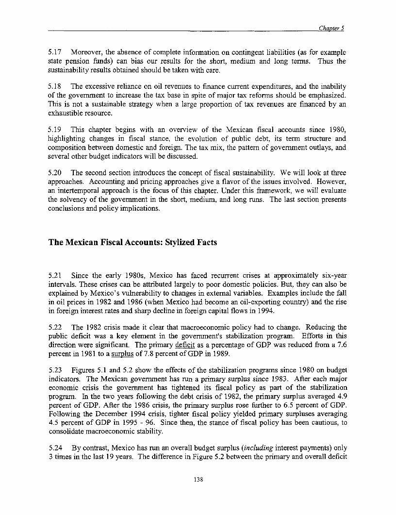
Chapter 5
5.17 Moreover, the absence of complete information on contingent liabilities (as for examplestate pension funds) can bias our results for the short, medium and long terms. Thus thesustainability results obtained should be taken with care.
5.18 The excessive reliance on oil revenues to finance current expenditures, and the inabilityof the government to increase the tax base in spite of major tax reforms should be emphasized.This is not a sustainable strategy when a large proportion of tax revenues are financed by anexhaustible resource.
5.19 This chapter begins with an overview of the Mexican fiscal accounts since 1980,highlighting changes in fiscal stance, the evolution of public debt, its term structure andcomposition between domestic and foreign. The tax mix, the pattern of government outlays, andseveral other budget indicators will be discussed.
5.20 The second section introduces the concept of fiscal sustainability. We will look at threeapproaches. Accounting and pricing approaches give a flavor of the issues involved. However,an intertemporal approach is the focus of this chapter. Under this framework, we will evaluatethe solvency of the govenmment in the short, medium, and long runs. The last section presentsconclusions and policy implications.
The Mexican Fiscal Accounts: Stylized Facts
5.21 Since the early 1980s, Mexico has faced recurrent crises at approximately six-yearintervals. These crises can be attributed largely to poor domestic policies. But, they can also beexplained by Mexico's vulnerability to changes in extemal variables. Examples include the fallin oil prices in 1982 and 1986 (when Mexico had become an oil-exporting country) and the risein foreign interest rates and sharp decline in foreign capital flows in 1994.
5.22 The 1982 crisis made it clear that macroeconomic policy had to change. Reducing thepublic deficit was a key element in the government's stabilization program. Efforts in thisdirection were significant. The primary deficit as a percentage of GDP was reduced from a 7.6percent in 1981 to a surplus of 7.8 percent of GDP in 1989.
5.23 Figures 5.1 and 5.2 show the effects of the stabilization programs since 1980 on budgetindicators. The Mexican government has run a primary surplus since 1983. After each majoreconomic crisis the government has tightened its fiscal policy as part of the stabilizationprogram. In the two years following the debt crisis of 1982, the primary surplus averaged 4.9percent of GDP. After the 1986 crisis, the primary surplus rose further to 6.5 percent of GDP.Following the December 1994 crisis, tighter fiscal policy yielded primary surpluses averaging4.5 percent of GDP in 1995 - 96. Since then, the stance of fiscal policy has been cautious, toconsolidate macroeconomic stability.
5.24 By contrast, Mexico has run an overall budget surplus (including interest payments) only3 times in the last 19 years. The difference in Figure 5.2 between the primary and overall deficit
138
Chapter 5
is the interest payments on the government domestic and foreign debt (as a percentage of GDP).Thus during the 1980s, the overall deficit was largely explained by interest payments.
5.25 Government debt as a percentage of GDP rose steadily between 1980 and 1986 and thenfell between 1986 and 1993. With the peso crisis of December 1994, debt to GDP once againincreased to the level of the early 1980s, owing to a jump in interest rates, but again started togradually fall by mid-1996 (see Figure 5.1).
Figure 5.1: Mexico Public Net Debt and Primary Deficit (+) as percentage of GDP 1980-98
:0
120.
80 S _ \ K
°198 198 198 rW 0 Ed19,80. , ,J 1993 1SS 198 i 1S97 1SA 190~T8 2a
IC PPMGDP
Source: SHCP
Figure 5.2: Mexico Overall and Primary Deficit (+) as percentage of GDP 1980-98
20
is
10
1980 1981 1982
u10 . -..----..-- - ,. ... ___.. . ...... . . . ......... _._. --. .... _. ....... . ... . . .....-.
DPPJMGDP _ECDEFGDPI
139

Chapter 5
Debt Management
5.26 Mexico's public debt, relative to GDP, fell from 115 percent in 1986-87 to about 26percent in 1998. This figure is low when compared to that of most of other OECD countries.
5.27 During the 1990s, Mexico has increasingly relied on foreign (as opposed to domestic)financing. As Figure 5.3 shows, in 1990, about 60 percent of government debt was foreign. By1998, this figure had risen to 80 percent (about 20 percent of GDP).
Figure 5.3: Mexico Domestic and Foreign Public Net Debt as percentage of GDP 1980-98
140-
120
100
SC 40
20
tsiS t96t 1 62 1400 o954 g1 0 6
A oq l 000 ,4AO 19940 %991 A9942 A993 I90 ,95 0990 A9t 0990
ForNgn ^T 00
Source: BoM
5.28 Following the peso crisis of December1994 the domestic debt management strategy hascentered on lengthening maturity and reducing interest payments. In particular, the maturity ofdomestic debt issued has increased.
5.29 Tesobonos, the dollar-linked short-term security that played a key role in the 1994 pesocrisis were eliminated in 1995. Instead, the Mexican authorities have increased the issuance of 1,2, and 3-year treasury bonds (BONDES). As a fraction of GDP, BONDES increased from 0.54percent in 1994 to 3.5 percent in 1998. Also, the recently introduced UDIBONOS, three andfive-year indexed bonds, now comprise about 1 1/2 percent of GDP. Together, as a fraction oftotal domestic debt outstanding, these two instruments comprised over two-thirds in 1998, upfrom 5 percent in 1994 (see Figure 5.4)
5.30 As another indication of longer maturity, foreign short-term obligations (less than oneyear) accounted for only 4.76 percent of Mexico's external public debt in December of 1998 (seeFigure 5.5).
140

Chapter 5
Figure 5.4: Public Sector Domestic Debt as percentage of GDP 1982-98
o AJUSTABONOS: 3and 5 year CPI-indexed securites
0 UDI8ONOS: 3, 5 and 10-year UDI-inked bonds (inflationindexed)
O BONDES: 1,2.3 and 10 year floatng rate bonds
* TESOBONOS: dollar-linked stort-tenn secuities (3, 6months, 1 year maturity)
10.00-0 CETES: 1 mrrnth to 2 -year-hued-rate treasury bills
9 00-
8.00- _
7.00-
6.00-
5.00-
2.00-3.00 XL- Z2eLSjE
0.001982 1983 1984 1985 1986 1987 1988 1989 1990 1991 1992 1993 1994 1995 1996 1997 1998
Source: SHCP
Figure 5.5: Mexico Public Foreign Debt, Term Structure 1982-1998
e5%
1t82 19t3 19#4 19S5 1983 1987 1#3 1989 1990 1991 1992 1993 1994 1996 1993 1997 1998
I M rATURITY OF I YEAR OR LONGER * MATURiTY OF LESS T-AN 1 YEAR
Source: SHCP
141

Chapter 5
Budget Indicators
5.31 Figure 5.6 shows the trends in Mexico's overall budget since 1980. Three elementsshould be noted. First, budgets are affected by oil prices,, as total revenues follow the cycle ofoil revenues quite closely.
5.32 Second, in response to this vulnerability to oil prices, the stance of fiscal policy remainedcautious, providing some margin of maneuverability in case of external shocks. The latter hasbeen achieved by running consecutive primary surpluses since 1983.
5.33 Third, the unpredictability of fiscal revenues as a consequence of its dependence on oilhas forced the government to make drastic expenditure cuts. As a fraction of GDP, non-interestexpenditures fell from about 25 percent in the 1980s to 19 percent in the 1990s, a drop of 23percent. Thus, the major adjustment in the 1990s came in the expenditure side of the budget. Bycontrast, non-oil revenue remained roughly constant at about 16.25 percent of GDP over thisperiod.
Figure 5.6: Mexico Budget Indicators as percentage of GDP 1980-1998
50o
45
40
35
30
25
20
15
10
1980 1981 1982 1983 1984 1985 1986 1987 1988 1989 1990 1991 1992 1993 1994 1995 1996 1997 1998
IITOTAL REVENUE =OILREVENUE TOTAL EXPENDITURE -4 NON INTEREST EXPENDITURES
Source: SHCP
142
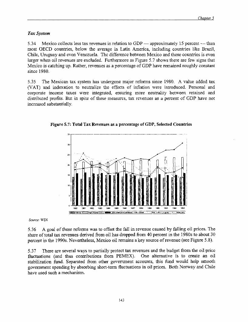
Chapter 5
Tax System
5.34 Mexico collects less tax revenues in relation to GDP - approximately 15 percent - thanmost OECD countries, below the average in Latin America, including countries like Brazil,Chile, Uruguay and even Venezuela. The difference between Mexico and these countries is evenlarger when oil revenues are excluded. Furthermore as Figure 5.7 shows there are few signs thatMexico is catching up. Rather, revenues as a percentage of GDP have remained roughly constantsince 1980.
5.35 The Mexican tax system has undergone major reforms since 1980. A value added tax(VAT) and indexation to neutralize the effects of inflation were introduced. Personal andcorporate income taxes were integrated, ensuring more neutrality between retained anddistributed profits. But in spite of these measures, tax revenues as a percent of GDP have notincreased substantially.
Figure 5.7: Total Tax Revenues as a percentage of GDP, Selected Countries
35
1 0i
1980 1981 1982 1993 1984 1995 1BM 1987 1999 1999 1998 1991 1992 1993
ljex r-= High innOECD _O CinL ,m Anbcea & C.-bs- -.- B- c19. - U V.fl
Source: WDI
5.36 A goal of these reforms was to offset the fall in revenue caused by falling oil prices. Theshare of total tax revenues derived from oil has dropped from 40 percent in the 1980s to about 30percent in the 1990s. Nevertheless, Mexico oil remains a key source of revenue (see Figure 5.8).
5.37 There are several ways to partially protect tax revenues and the budget from the oil pricefluctuations (and thus contributions from PEMEX). One alternative is to create an oilstabilization fund. Separated from other government accounts, this fund would help smoothgovernment spending by absorbing short-term fluctuations in oil prices. Both Norway and Chilehave used such a mechanism.
143

Chapter 5
Figure 5.8: Oil Revenues as a percentage of Total Government Revenues
Souce: SHCP
5.38 Another key revenue source for many developing countries is base money creation, orseignorage. As Figure 5.9 shows, seignorage has steadily decreased as source of revenue inMexico. Between 1986 and 1998, seignorage as a share of total tax revenue fell from 10 percentto about 3 percent. As a fraction of GDP, seignorage fell from about 3.5 percent in 1986 to 0.6in 1998.
Figure 5.9: Seignorage as a Source of Revenue
12.00 _ _ _ _ __ _ _ _ _ _
10 00
0.00
6.00
4.00
2.00
70.X0
1 *C0 1007 100 1099 1090 1991 1992 19 93 1994 90 109 6 1 09 7 16 9
ICSEIGNORAGE /TOTAL REVENUE -0-SEIGNORAAIE GOP
Source: BoM
5.39 Excluding oil revenues, the tax mix in Mexico does not stand as unusual when comparedto other OECD and Latin American countries, as Figure 5. t 0 shows.
144

Chapter 5
5.40 VAT revenues have remained almost unchanged as the rise in VAT rate from 10 to 15percent in 1995 offset the drop in real private consumption and imports from the peso crisis.
5.41 There has been an increasing reliance since the 1980s on excise taxes, whereas taxes oninternational trade have become less important, in part due to the trade liberalization that startedin 1986 and culminated with the NAFTA agreement.
5.42 The primary non-income tax source is the contribution of PEMEX and subsidiaries to thefederal government through a hydrocarbons fee. The hydrocarbons fee paid by PEMEX to thefederal government is comprised of an oil extraction royalty, the regular income tax, and anexcise tax. This is approximately 61 percent of gross revenues excluding VAT. PEMEX alsocontributes to the federal government paying ordinary VAT payments and customs duties, aswell as an "excess profit fee" on windfall gains from oil exports.
Figure 5.10: Federal Government Revenue Tax Mix
100%
80!
60%
40%
20%
0%1980 1981 1982 1983 1984 1985 1986 1987 1988 1989 1990 1991 1992 1993 1994 1995 1996 1997 1998
ISINCOMETAX MVALUEADDEDTAX OEXCISETAX 0 TAXESONINTERNATIONALTRADE UOTHERINCOMETAXES ONON:INCOME TAX
Source: SHCP
145

Chapter 5
Government Expenditure Composition
5.43 In comparison to OECD and Latin American countries, Mexican governnent expenditureas a fraction of GDP is relatively low. This is mainly the response to the low tax revenues andthe need for a prudent fiscal policy (see Figure 5.1 1). More public spending to enhance capacityin areas like education, health, infrastructure and poverty alleviation are desirable, but thefinancing of these expenditures will require a larger tax base.
5.44 Figures 5.12 and 5.13 show the evolution of government expenditure and its compositionsince 1980. The several fiscal adjustments taken place in the last decades have cut substantiallygovernment expenditures. One of the components most affected has been real capitalexpenditure, which fell by 23 percent between the 1980s and the 1990s. By contrast, salaries andwage have declined only about 4.6 percent over the same period.
5.45 Interest payments on public debt fell from 45.5 percent of total expenditures in 1987 toabout 13.5 percent in 1998. This reflects of decline in the public debt and a cautious debtmanagement that includes an increase in average debt maturity. This policy has helped shieldMexico from short-term interest rate movements.
Figure 5.11: Total Expenditure of the Central Government as a percentage of GDP,Selected Countries
40
35
30
25
20
15
10
5
' a1S80 1981 1982 1983 1984 1985 1988 1987 1988 1989 1990 1991 1992 1993
l high ina. OECinLatn Ar-enca & Canbbea=Me,co Mi rBil -s Chile - UWwy -- Venezuel
Source: WDI
5.46 The transfer component of total expenditure has increased since the 1980s by 82 percent.As a fraction of total expenditures, transfers rose from 14.2 percent in 1980 to almost 30 percentby 1998, reflecting a commitment of the Mexican government to reduce poverty.
146

Chapter 5
5.47 Finally the revenue shared with state government has doubled in the last two decades,representing the increasing decentralization of government spending to states and municipalities.
Figure 5.12: Total Government Expenditure (in Mill of $ 94 mxp)
180000
160000
140000
120000
100000
80000
60000
40000
01980 1981 1982 1983 1984 1985 1986 19e7 1988 1989 1990 1991 1992 1993 1994 1995 1996 1997 1998r--1 nterest Payments _Capital expenditure rTransfers|_Reve3nue shared with state govemmfents --m Salares and wages Materials and supplies
Other crraent expenditure -ADEFAS
Source: SHCP
Figure 5.13: Expenditure Composition
100%
60% ;
40%O_
% I1980 1981 1982 1983 1984 1985 1986 1987 198a 1989 1990 1991 1992 1993 1994 1995 1996 1997 1998
3 = = D aaealnds ges * ad t pns ard sOther c.menr e96eMd6urjlCorp1al expenditure STranr.ters ORenele SIshated witth state govemrnents* ADEFAS OT nRedenh Pavmn-rs ,
Source: SHCP
147
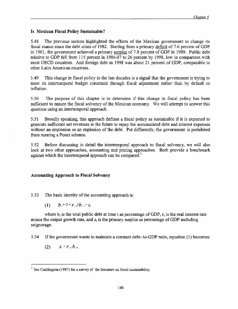
Chapter 5
Is Mexican Fiscal Policy Sustainable?
5.48 The previous section highlighted the efforts of the Mexican government to change itsfiscal stance since the debt crisis of 1982. Starting from a primary deficit of 7.6 percent of GDPin 1981, the government achieved a primary surplus of 7.8 percent of GDP in 1989. Public debtrelative to GDP fell from 115 percent in 1986-87 to 26 percent by 1998, low in comparison withmost OECD countries. And foreign debt in 1998 was about 21 percent of GDP, comparable toother Latin American countries.
5.49 This change in fiscal policy in the last decades is a signal that the government is trying tomeet its intertemporal budget constraint through fiscal adjustment rather than by default orinflation.
5.50 The purpose of this chapter is to determine if this change in fiscal policy has beensufficient to ensure the fiscal solvency of the Mexican economy. We will attempt to answer thisquestion using an.intertemporal approach.
5.51 Broadly speaking, this approach defines a fiscal policy as sustainable if it is expected togenerate sufficient net revenues in the future to repay the accumulated debt and interest expenseswithout an implosion or an explosion of the debt. Put differently, the government is prohibitedfrom running a Ponzi scheme.
5.52 Before discussing in detail the intertemporal approach to fiscal solvency, we will alsolook at two other approaches, accounting and pricing approaches. Both provide a benchmarkagainst which the intertemporal approach can be compared.'
Accounting Approach to Fiscal Solvency
5.53 The basic identity of the accounting approach is:
(1) b, = ( + r,) b, -s,
where bt is the total public debt at time t as percentage of GDP, rt is the real interest rateminus the output growth rate, and st is the primary surplus as percentage of GDP includingseignorage.
5.54 If the government wants to maintain a constant debt- to-GDP ratio, equation (1) becomes:
(2) s,=r,,b,,
See Cuddington (1997) for a survey of the literature on fiscal sustainability
148

Chapter 5
Thus if the government wants to keep fully servicing its debt without increasing its debt to GDPratio, its primary surplus including seignorage as percentage of GDP has to be at least equal tothe real interest rate minus the output growth rate of the economy.
5.55 For example, take the case of Mexico in 1998
Table 5.1: Accounting Approach Mexico in 1998
bt tt-gt Seignorage st rt
25.9% 1.67% 0.60% 2.27% 8.76%
Source: Author's calculations
The stock of public debt outstanding at the end of the period was 25.9 percent of GDP; theprimary surplus inclusive seignorage was 2.3 percent of GDP. Thus, according to equation 2, thegovernment is solvent if the creditors are willing to accept securities at a real interest of 8.76percent plus the output growth rate. This figure appears quite feasible, in light of annual ex-postreal interest rates on CETES averaging around 6 percent in 1998. It should be noted that thisback of the envelope calculation for the Mexican economy omits contingent liabilities such asFOBAPROA.
Pricing Approach to Fiscal Solvency
5.56 Another proxy for fiscal sustainability is the market price of the government debt.Forward looking investors will require a discount on purchases if they anticipate a problem ofsolvency.
5.57 As discussed in the section on fiscal accounts, Mexican investors trade governmentsecurities in two markets, the secondary market for sovereign debt and the domestic treasurybills market.
5.58 Figures 5.14 and 5.15 show the discount at which both types of debt are traded. The ex-post real rates of return on short-term peso denominated treasury bills, CETES, have fluctuatedenormously since 1985. At the highest end, in February 1988 the real annualized interest ratewas 127.64 percent. Since the peso crisis, when the real annual rate peaked in April 1995 at 37percent, the real annualized interest rate has fallen steadily. This suggests increasing confidencein the fiscal solvency of the Mexican government.
5.59 In the external market, the discounts on Brady bonds have also reflected the fiscalproblems of the Mexican economy. In the midst of the peso crisis, March 1995, Brady bonds
149

Chapter 5
were trading at 56 percent of their value. Since then the price has increased steadily with theexception of August 1998, on the heels of the Russian default.
5.60 Another indicator of fiscal sustainability used in the literature is the country credit ratingsand sovereign spreads. Figure 5.16 shows the J. P. Morgan EMBI spread. Mexico's countryspread is below the average for Latin America (including Brazil), and has decreased steadilysince the peso crisis with the exception of the period between the East Asia crisis and theRussian default.
Figure 5.14: Real Annualized Interest Rate Figure 5.15: Brady Bonds DiscountCETES 28 days
100 ------
80
70
Source: BoM Source: Bloomberg
5.61 Drudi and Prati (1999) present a signaling model in which primary surplus andoutstanding debt are complementary inputs in the determnination of the credit rating of a country.An increase in the debt to GDP ratio or an improvement in the primary surplus is expected toraise the rating. One of these credit rating indicators is the Institutional Investor rating publishedtwice a year since 1979. Banks are asked to grade each of the countries on a scale of 0 to 100,with 100 representing those with least chance of default. Figure 5.17 shows the InstitutionalInvestor rating for Mexico. It has trended upward steadily since 1979 with the exception of thepeso crisis.
150
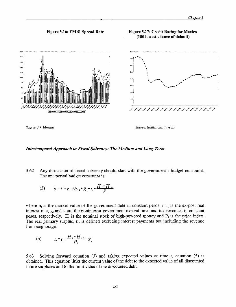
Chapter 5
Figure 5.16: EMBI Spread Rate Figure 5.17: Credit Rating for Mexico(100 lowest chance of default)
iilSt,lili 3iqlitila - - -- i---
S5ource: J.P. Morgan Source: Institutional Investor
Intertemporal Approach to Fiscal Solvency: The Medium and Long Term
5.62 Any discussion of fiscal solvency shou0d start with the governrent's budget constraint.The one period budget constraint is:
(3) b, = G + r,-,) b,-, + H, -H,, 9 ,
where bt is the market value of the govenment debt in constant pesos, r t-m iS the ex-post realinterest rate, gt and tt are the noninterest government expenditures and tax revenues in constantpesos, respectively. Ht is the nominal stock of high-powered money and Pt is the price index.The real primary surplus, st, is defined excluding interest payments but including the revenuefrom seignorage.
(4) s,=t,+ H,-HI, gPI
5.63 Solving forward equation (3) and taking expected values at time t, equation (5) isobtained. This equation links the current value of the debt to the expected value of all discountedfuture surpluses and to the limit value of the discounted debt.
151

Chapter 5
(5) b,= 1 E,Si-limEv'=(- ' (l+r)
5.64 The present value constraint requires that in equation (5), b, equals only the first term onthe right hand side. That is, that the sum of all future surpluses are expected to be sufficient torepay the current outstanding debt. This implies that the following condition must be satisfied:
(6) b, E, s,=l(l+r)
Equivalently, the second term in equation (5) must equal zero.
(7) lim E, b -vN- (I (+r)
this condition rules out explosive debt bubbles, and is thus called the non-Ponzi game condition.
5.65 To summarize, according to the government's intertemporal budget constraint, thecurrent real value of its liabilities, bt, must by definition equal the present value of future primarysurpluses (taxes minus non-interest expenditures). Restating more simply, for fiscal policy to besustainable, a government that has debt outstanding must anticipate that sooner or later it willhave to run primary surpluses. Those surpluses must be large enough to satisfy equation (6).
5.66 Suppose that in equation (6) the right-hand side is much below the left-hand side. Thiswould suggest that sooner or later the government would need to increase its primary surplusthrough taxes or reductions in spending. Barring that, the governnent would have to eventuallyeither monetize or repudiate its debt.
5.67 Equation (6) suggests a number of ways to assess fiscal sustainability in an intertemporalset-up. The difficulty resides in forecasting primary surpluses into the future; two methodologieswill be discussed. In the next section we will address the fiscal sustainability of Mexico in theshort and medium term. This fiscal solvency exercise is an application of Blanchard (1990).
The short and medium term
5.68 Blanchard (1990) suggests as an index of sustainability the gap between t and t*, where tis the ratio of tax revenue to GDP and t* is the sustainable tax rate. t is computed by recallingthat the primary surplus st equals tt-gt. Replacing in equation (6) to solve for the constantsustainable rate, t we get
(8) t =(r-) 1bo
152
Chapter 5
where all variables are normalized by GDP. r is the real interest rate, 0 is the GDP growth rate,g, is the noninterest government expenditure to GDP, and bo the initial debt to GDP.
5.69 The sustainable tax rate is equal to the present value of the expected future noninterestgovernment spending, plus the difference between the ex-ante real interest rate and the growthrate times the ratio of debt to GDP. If t* is greater than the current tax rate t, then taxes will haveto increase or spending to decrease. The gap (t* -t) is the size of the adjustment.
5.70 Note that a positive value in (t*-t) does not imply that taxes should be increased. Theindex is symmetric in the sense that the treatment of taxes and spending is equivalent. Theadjustment can come from taxes, spending cuts or both.
5.71 The simplicity and appeal of this indicator is that it can be implemented for finite timeperiods, such as 1 year or 5 years. Table 5.2 reports the results of this exercise. The initialconditions are those prevailing in 1998.
5.72 The first and third column show the extent of the adjustment needed in the case wheregovernment expenditures to GDP remained constant at the 1998 level and the bailout ofFOBAPROA is not taken into account. The difference in the extent of the adjustment is theassumption made about the path of the real interest rate minus GDP growth (discount rate).
5.73 The one-year as well as the 8-year projection show a negative gap for a discount rate of 5and 3 percent. Thus there is room for an increase in government spending between 0.5 and 0.8percent of GDP.
5.74 However the gap becomes positive once the bailout figures are taken into consideration.Assuming a discount rate of 5 percent, the government will have to increase taxes or reducegovernment spending from 1999 to 2006 between 0.3 and 0.8 percent of GDP. If the discountrate is 3 percent, this will be only necessary in 2005 and 2006 in an amnount of 0.1 percent ofGDP.
5.75 Following the OECD's (1999) estimate, the previous exercise assumes a cost of thebailout of FOBAPROA around 14.4 percent of the GDP. Of this amount 3.2 percent has beenalready disbursed, including 0.3 in 1998. The remainder is assumed to be disbursed equally inthe next years.
5.76 The numbers obtained from this simple exercise seem plausible and barely affect theoverall solvency of the Mexican government. As a cautionary note, due to data limitations thisexercise does not include all contingent liabilities. For example, since the implementation of thesecurity reform of 1997 contributions formerly made to the IMSS are lower, and are nowchanneled to private fund managers. This lower revenue will start to put pressure on the budgetbalance, as higher expenditures to fill the gap will be needed.
153
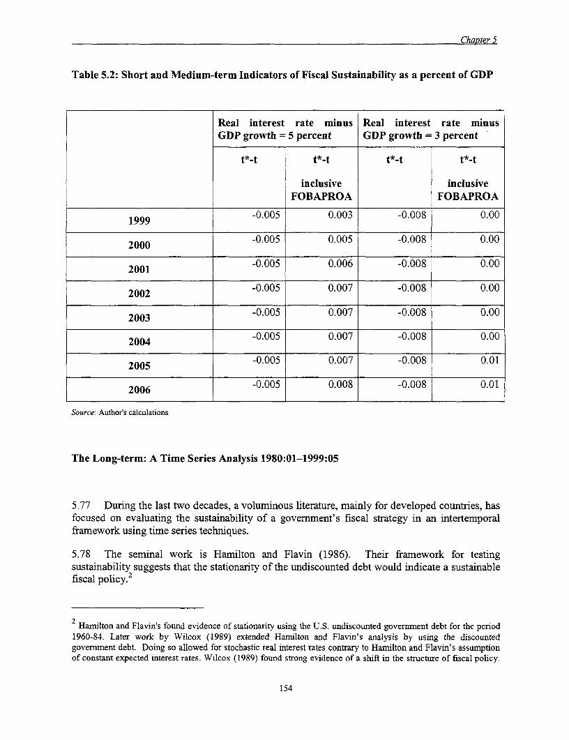
Chapter 5
Table 5.2: Short and Medium-term Indicators of Fiscal Sustainability as a percent of GDP
Real interest rate minus Real interest rate minusGDP growth -5 percent GDP growth = 3 percent
t*-t vI t*-t t*-t t*-t
inclusive inclusiveFOBAPROA FOBAPROA
1999 -0.005 0.003 -0.008 0.00
2000 -0.005 0.005 -0.008 0.00
2001 -0.005 0.006 -0.008 0.00
2002 -0.005 0.007 -0.008 0.00
2003 -0.005 0.007 -0.008 0.00
2004 -0.005 0.007 -0.008 0.00
2005 -0.005 0.007 -0.008 0.01
2006 -0.005 0.008 -0.008 0.01
Source: Author's calculations
The Long-term: A Time Series Analysis 1980:01-1999:05
5.77 During the last two decades, a voluminous literature, mainly for developed countries, hasfocused on evaluating the sustainability of a government's fiscal strategy in an intertemporalframework using time series techniques.
5.78 The seminal work is Hamilton and Flavin (1986). Their framework for testingsustainability suggests that the stationarity of the undiscounted debt would indicate a sustainablefiscal policy.2
2 Hamilton and Flavin's found evidence of stationarity using the U.S. undiscounted govermnent debt for the period1960-84. Later work by Wilcox (1989) extended Harnilton and Flavin's analysis by using the discountedgovemment debt. Doing so allowed for stochastic real interest rates contrary to Hamilton and Flavin's assumptionof constant expected interest rates. Wilcox (1989) found strong evidence of a shift in the structure of fiscal policy.
154

Chapter 5
5.79 Hakkio and Rush (1991), Haug (1991), Smith and Zin (1991) and Trehan and Walsh(1991) developed an alternative framework to test the borrowing constraint. Their test forsustainable fiscal policy relied on co-integration of tax revenues, expenditures and governmentdebt. 3
5.80 The next sections will apply unit root as well as cointegration tests to several indicatorsof fiscal policy in Mexico. For developing countnres the literature of fiscal sustainability in anintertemporal framework is scarce, and hopefully this exercise will broaden our understanding ofthe mechanisms used by developing countries to satisfy their intertemporal budget constraint.4
5.81 It should be kept in mind that our discussion of the long term sustainability will not takeinto account contingent liabilities as we did in the short and medium exercise.
Testing the Intertemporal Budget Constraint: Unit Roots
5.82 Table 5.3 shows the results for the Mexican economy using monthly data of undiscounteddebt from 1980:01 to 1999:05. The Augmented Dickey-Fuller test (ADF) with a drift and atrend tern shows that at a 5 percent level we reject the hypothesis of nonstationarity. TheMexican government is not running a Ponzi scheme.
For the period prior to 1974, he found no evidence of violation of the borrowing constraint. However, after 1974 thestationarity of the discounted debt failed to hold.
3 Trehan and Walsh (1991) and Haug (1991) supported Hamilton and Flavin's results for the full sample. Haugfound that priraary deficit and debt are co-integrated. Trehan and Walsh found the same result using governmentspending inclusive of interest payments and government revenue including seignorage. Hakkio and Rush (1991)imposing breaks obtained similar results to those of Wilcox. Smith and Zin (1991) using Canadian data tested forthe co-integration of government debt and primary deficit and found that the government does not obey the presentvalue constraint. Ahmed and Rogers (1995) tested whether the U.S. and U.K. economic policies are consistent withthe intertemporal budget constraint and external borrowing constraint. They found that the present value constraintholds over the whole sample for the government using government revenue, government spending exclusive ofinterest payments, and interest payments as co-integrating series.
4Tanner (1994, 1995) and Rocha (1997) analyze the case of Brazil. Werner (1992) and Solis Sober6n andVillag6mez (1999) analyze the case of Mexico.
155

Chapter S
Table 5.3: Testing for Nonstationarity in Undiscounted and Discounted NetPublic Debt, 1980:01-1999:05
Abt = r + Strend + (p - I)b t - + k cjAbt -1+ pt
Undiscounted debt Discounted debt(1) bt -0.07 (0.02) (4) btI -0.07 (0.03)
c 58.06 (16.25) c 37.19 (13.97)trend -0.18 (0.05) trend -0.18 (0.07)lags 24 lags 24ADF -3.42 ADF -2.81AIC 9.57 AIC 8.58
(2) b, -0.05 (0.01) (5) bI -0.06 (0.02)c 37.28 (10.53) c 30.48 (9.16)
trend -0.12 (0.04) trend -0.15 (0.04)lags 12 lags 12ADF -3.47 ADF -3.46*AIC 9.44 AIC 8.46
(3) bt- -0.04 (0.01) (6) b,_1 -0.06 (0.02)c 33.81 (3.41) c 29.42 (8.46)
trend -0.10 (0.03) trend -0.14 (0.04)lags 10 lags 10ADF -3.30 ADF -3.61AIC 9.43 AIC 8.44
Note:ADF is the augmented Dickey-Fuller test statistic.Statistics rejecting nonstationarity at the critical 5 percent level are marked by * and those rejectingat I percent by **.AIC is the Akaike information criterion.Conventionally standard errors are in parentheses.All equations have been checked for auto-regressive errors up to the fourth order.
The Case of a Stochastic Discount Rate
5.83 The previous analysis relies on a very restrictive assumption, namely that the real interestrate is constant. To account for a stochastic discount factor, a testing strategy was first proposedby Wilcox (1989). According to this test, it should be verified that the discounted debt timeseries is stationary and its steady-state value be zero. The discount factor was determined as inCorsetti and Roubini (1991). The share of interest expenses in the domestic and external debtstock was weighted by the importance of domestic and external debt in the total debt. This termgive us a proxy for the nominal discount rate for the total debt. Finally, the discounted factor dtwas computed as:
(9) d f li, o,=o 1 + 2Z v,1
156

Chapter S
5.84 Table 5.3 presents the results for the stationarity of the discounted debt. Interestingly, theADF are not very different from the ones obtained for the undiscounted debt. The nullhypothesis of a unit root can be rejected at 5 percent. Thus, the assumption of constant interestrates does not seem to affect the results drastically.
5.85 Before adopting the aforementioned results, we need to investigate the presence of astructural break or breaks in the time series representation of the undiscounted and discounteddebt.
Testing for a change in regime
5.86 Another central issue in the evaluation of the sustainability hypothesis using unit roottests is detecting the presence of a structural break or breaks in the time series representation ofthe public debt. Solis Sober6n and Villag6mez (1999) found evidence of a break in theundiscounted and discounted debt series in the third quarter 1988. The Mexican public debt wasin an explosive path before 1988:3.
5.87 Figure 5.18 shows two changes in the slope of its trend, one in 1988-89 and anothertoward the end of the period.
Figure 5.18: Mexican Net Public Debt, 1980:1-1999:5
Undiscounted at Market Value(in Bill. of $94 mxp)
1000.00
900.00
MeOO.D
700.00
600.00
400.00
400.00 ,/
200.0013
100.00
0.00
- [TDomesticDebt -F0eignDebt -Total Debt
Source: BoM
157
Chapter 5
5.88 At the univariate level the most commonly used test for a constant shift or a trend shift isPerron (1989). Perron's test involves the introduction of appropriately defined dummy variablesin the ADF auxiliary regression. This will allow testing for unit roots with a shift in the mean orthe slope of the trend coefficient. However, Perron's procedure is conditional on a known breakpoint.
5.89 Zivot and Andrews (1992) have proposed a class of tests that circumvents the bias thatresides with the selection of the dates with a priori information. These tests incorporate theestimati on of a break point into the testing procedures using sequential methods (full samplewith dummies). The breakpoint selection procedure relies on identifying the breakpoint thatproduces the lowest value over all possible breakpoints of the relevant one-sided unit root tstatistic denoted by t(X), where X. stands for the break fraction in the sample.
5.90 The Augmented Dickey-Fuller auxiliary regression proposed by Zivot and Andrews canbe written as:
bt + (DUt(2)+ 5DT,(2)+&trend+pb- i+T. IcAbr-ie=
where t=1, 2.T, T =ib and Tb is the break pointT
lift> TA. t-TA if t>TlDUjt(X) = I., DTtQ.) =L0 otherwise o otherwise
5.91 The estimation of the auxiliary regression is performed sequentially with the breakpoint
T= t assuming values in the range ~ (0.15,0.85). In our case it means that we will test forT
breaks in the series between 1982:11 and 1996:06.
5.92 The estimation of this general formulation may be used to evaluate the alternativehypothesis of stationarity around a segmented deterministic trend and/or a shifting mean. Usingthe Zivot and Andrews' procedure we allow for the endogenous determination of structuralbreaks in the Mexican discounted and undiscounted debt. The sequence of unit root t-ratios arereported in Figure 5.19
5.93 Figure 5.19 shows the evolution for t(X). We can think of t(X) as an ADF once the breaksare incorporated explicitly. In that sense a movement to lowest values indicates a possible breakin the series. In the case of the undiscounted debt the break is December 1989 with a t(X) valueof-3.81. But the t test is below the critical value in Zivot and Andrews5. Thus the break is not
5 Table 4 in Zivot and Andrews show a critical value of -5.08 at 5 percent level and -5.57 at 1percent.
158

Chapter 5
significant. The undiscounted debt is, according to this test, absent of breaks. One caveat tokeep in mind is the low power of these tests in small samples.
Figure 5.19: Sequential Zivot-Andrews Unit Root Test for the Mexican Undiscounted andDiscounted Public Net Debt, 1980:1-1999:5
0 00
.uo 141 5p 4<iA5' 9b<Sb 9b *9> oleb b<5>* SI ,6 5;V5 9
-0.60
-0.80
-1.002
-1.20 -
-1.40.. ,
''Y°~~~~ti 10 Ctt,IVa
-2.60 5_
*X1.
'52.00
|_-Z-A ADF t5tetUldiSCOUetd Debt --- Z-A ADF StteStOUsonIed Dbt|
5.94 For the discounted debt the path is similar. The lowest valued for t(R) is -4.52 in January1990, but is above the threshold to accept a break. Table 5.4 shows the auxiliary equationsestimated for the undiscounted and discounted debt.
5.95 In summary, tests for unit roots in the undiscounted and discounted public debt tell usthat we can reject at the 5 percent level that the Mexican government since 1980 has followed anunsustainable path in their fiscal policies. Breaks in the series do not seem to play any role.6
6. Solis Sober6n and Villagomez (1999) found evidence of a break in the undiscounted and discounted debt seriesin the third quarter 1988. However their data end in the last quarter of 1997, and the test used is Perron whichassumes an a priori date for the break.
159
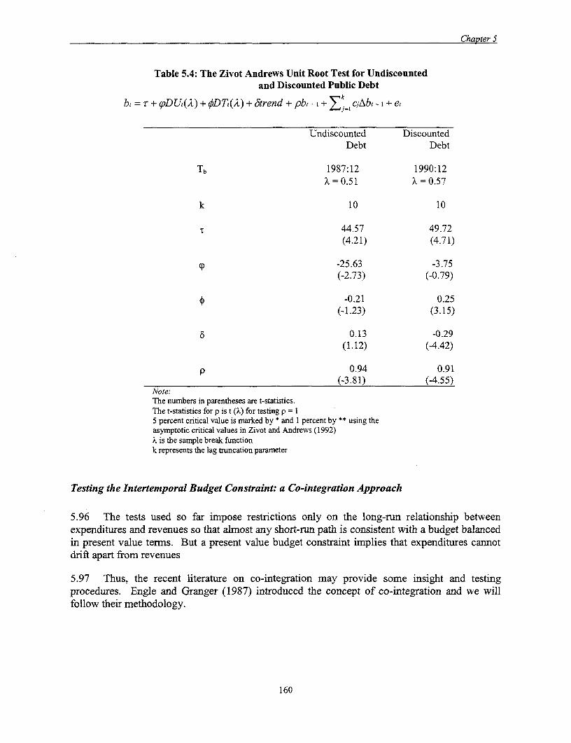
Chapter S
Table 5.4: The Zivot Andrews Unit Root Test for Undiscountedand Discounted Public Debt
bt = r + oDUt(A) + bDTt(A) + Strend + pbt -1 + E cAb= -,+ e
Undiscounted DiscountedDebt Debt
Tb 1987:12 1990:12X = 0.51 X = 0.57
k 10 10
Tr 44.57 49.72(4.21) (4.71)
,p -25.63 -3.75(-2.73) (-0.79)
(p -0.21 0.25(-1.23) (3.15)
6 0.13 -0.29(1.12) (4.42)
p 0.94 0.91(-3.81) (-4.55)
Note:The numbers in parentheses are t-statistics.The t-statistics for p is t (X) for testing p = I5 percent critical value is marked by * and I percent by ** using theasymptotic critical values in Zivot and Andrews (1992)X is the sample break functionk represents the lag truncation parameter
Testing the Intertemporal Budget Constraint: a Co-integration Approach
5.96 The tests used so far impose restrictions only on the long-run relationship betweenexpenditures and revenues so that almost any short-run path is consistent with a budget balancedin present value terms. But a present value budget constraint implies that expenditures cannotdrift apart from revenues
5.97 Thus, the recent literature on co-integration may provide some insight and testingprocedures. Engle and Granger (1987) introduced the concept of co-integration and we willfollow their methodology.
160

Chapter 5
Testing Long-run Relationship Between Government Spending Inclusive of Interest Paymentsand Revenue7
5.98 We will perform the test suggested by Hakkio and Rush (1991), investigating co-integration of government spending, inclusive of interest and govenment revenues. Govemmentspending and revenues cannot drift away if the intertemporal budget constraint holds.
5.99 Hakkio and Rush derived their test assuming a stationary real interest rate. Thus, weneed first to venrfy the behavior of monthly real interest rates. The forrnal results are presentedin Table 5.5. We reject the hypothesis of unit root at a 1 percent level. The real interest rateseries exhibits a tendency to return to a constant mean.
5.100 Once we established the stationarity of the real interest rates, we can use undiscountedvariables and apply the Engle and Granger methodology. The first step is to test for stationarityin government spending inclusive of interest and government revenues. Figure 5.20 shows theplot of both series and Table 5.6 the stationary tests for levels and first differences.
Table 5.5: Testing for Nonstationarity in Real Interest Rates, 1980:1-1998:07
Art = Tr + trend + (p - 1)rt- + k cArt - i +,ut
1980:01-1998:07(l) ~~~bt-I -0.08 (0.02)
c -1.27 (1.06)trend 0.01 (0.01)lags 2ADF -3.69AIC 6.84
(2) bt -0.07 (0.02)c 0.12 (0.49)
lags 2ADF -3.37AIC 6.84
(3) b,.1 -0.07 (0.02)lags 2ADF -3.37**AIC 6.83
Note:ADF is the augmented Dickey-Fuller test statistic.Statistics rejecting nonstationarity at the 5 percent critical level are marked by * and thoserejecting at I percent by **.AIC is the Akaike information criterionConventionally standard errors are in parentheses.All equations have been checked for auto-regressive errors up to the fourth order.
7. In the rest of the paper only the ADF statistic will be reported. The Phillips-Perron statistic rejects the nullhypothesis of unit root as high as 99.7 percent of the time if the MA representation of the error is negative equalsto -0.8. In our case the range is ftom -0.6 to - 0.8. See Banerjee, Dolado, Galbraith and Hendry (1994) pp. 113.
161

Chapter 5
5.101 The hypothesis of nonstationarity cannot be rejected at the 5 percent level for bothgovernment expenditures inclusive of interest payments and govermment revenues. However,when measured as first differences, these variables are stationary. Thus, the co-integration test isadequate.
5.102 The co-integration test implies to check the residuals of the long-run regression forstationaiity. The results are presented in Table 5.7. The co-integration test does not reject thehypothesis of non-co-integration at the 5 percent level.
Table 5.6: Testing for Nonstationarity in Real Government Spending InclusiveInterest Payments and Government Revenues, 1980:1-1999:05
Levels FirstDifference
ADF Lags ADF LagsGovernment -1.70 24 -6.22** 12Expenditure
inclusiveinterest
Govenmment -2.23 23 -10.31 10Revenue
Budget Deficit -5.11** 24 -9.65** 12Note:ADF is the augmented Dickey-Fuller test statistic.Statistics rejecting nonstationarity at the 5 percent critical level are markedby * and those rejecting at 1 percent by **.
Table 5.7: Results of Co-integration Government Spending Inclusive Interest Paymentsand Government Revenue, 1980:01- 1999:05
tt= a + b ggt +tt
ADF Lagst/gg -2.63* 24
-2.10* 12Note:
ADF is the augmented Dickey-Fuller test statistic.Statistics rejecting non co-integration at 5 percent critical level are marked by * and thoserejecting at I percent by .
162

Chapter 5
Figure 5.20: Government Spending Inclusive Interest Payment and Government Revenues:1980:01-1999:05 (in Bill. P$94)
60.00
00.00
40.00
20.00
20.00 .
1000
0.00
.- Primary Revenue (Bill PF 94) -0- Spening inclusive Interest Payments (Bdl P5 94)
Source: SHCP
5.103 An additional issue raised by Hakkio and Rush was whether the co-integrating factor bequals 1. Although a value less than one is consistent with a strict interpretation of theintertemporal budget constraint, it implies increasing difficulties in marketing the debt. One wayto test for b=1 is to examine the stationarity of the differences between spending inclusiveinterests and revenue (deficit).
5.104 The deficit constrains the parameters of the co-integrating regression to a=70 and b=1.Table 5.6 presents the results. The nonstationarity of the deficit is rejected at the 1 percent level.Hence, we conclude the deficit is stationary, and the government is fiscally solvent.
Testing Long-run Relationship Between Government Spending Exclusive of InterestPayments, Interest Payments and Revenue
5.105 Ahmed and Rogers (1995) use the co-integration between government spendingexclusive interest payment, interest payments, and governnent revenue as evidence that thegovernment intertemporal budget constraint holds. Figure 5.21 shows the path of the threeseries. Tables 5.8 and 5.9 show the results for stationarity and co-integration.
163

Chapter 5
Table 5.8: Testing for Nonstationarity in Real Government Spending, Interest Payments andGovernment Revenues, 1980:1-1999:05
Levels First DifferenceADF Lags ADF Lags
Government Expenditure -2.58 23 -4.22** 24
Government Revenue -2.23 23 -10.31 10
Interest Payments -2.93 24 -7.33 10Note:ADF is the augmented Dickey-Fuller test statistic.Statistics rejecting nonstationarity at the 5 percent critical level are marked by * and those rejectingat 1 percent by **.
Table 5.9: Results of Co-integration Noninterest Government Spending, InterestPayments and Government Revenue, 1980:01- 1999:05
ti= a + b gt + c rbt+pt
ADF Lagst/g,rbt -3.32** 24
Note:ADF is the augmented Dickey-Fuller test statisticStatistics rejecting non co-integration at the 5 percent critical level are marked by * and thoserejecting at I percent by **
Figure 5.21: Government Spending, Interest Payments and Government Revenues:1980:01-1999:05 (in Bill. P$94)
60.00
50.00
40.00, _
0.0
PSb t9 9 9 oP P; eP Pb/ P P 9 t .1' 9 9 1 ¢9 + 9 <9 9
lnterest Paymemn (Bil PS 94) Pinary Speding (Bill PS 94) Ptnmary Revenue (BiD PS 94)
Source: SHCP
164

Chapter 5
5.106 The results show that noninterest governnent spending, interest payment and governmentrevenue are co-integrated. The three variables move together and they adjust to a long-runrelationship, so their difference does not drift apart. The stationarity of the deficit assures us thatthe co-integrated vector is (1,,-1).8 For developing countries, this test gives an insight on theimportance of interest payments. The co-integration of g, t and rb indicate that Mexico hasresponded to the increase in interest payments by increasing primary surpluses.
Policy Conclusions
5.107 The main results of this paper can be summarized as follows:
5.108 Budgets are affected by oil prices, as total revenues follow the cycle of oil revenues quiteclosely. In response to this vulnerability to oil prices and the effect of interest rates, the stance offiscal policy has remained cautious. The latter has been achieved by running consecutiveprimary (interest exclusive) surpluses since 1983.
5.109 This primary surplus has been obtained primarily by drastic expenditure cuts. As afraction of GDP, non-interest expenditures fell from about 25 percent in the 1980s to 19 percentin the 1990s, a drop of 23 percent. By contrast, non-oil revenue remained roughly constant atabout 16.25 percent of GDP over this period. In particular, the major adjustment in the 1990scame from capital expenditure.
5.110 Mexico's public debt, relative to GDP, fell from 115 percent in 1986-87 to about 26percent in 1998, due to primary surpluses and a debt management strategy centered onlengthening maturity and reducing interest pavments after the peso crisis.
5.111 The short and medium tern projections of fiscal sustainability using an intertemporalapproach for the Mexican economy between 1999-2006 show that the required adjustment in theprimary surplus will be around -0.5 and -0.8 percent of GDP. The government can increasegovernment spending or reduce taxes. This under the assumption that government expendituresto GDP remained constant at the 1998 level and the bailout of FOBAPROA is not taken intoaccount.
5.112 However, results change if FOBAPROA bailout is included. Assuming a discount rate of5 percent, the government will have to increase taxes or reduce government spending in the nextyears approximately between 0.3 and 0.8 percent of GDP. If the discount rate is 3 percent thisadjustment will be only necessary in 2005 and 2006 for an amount of 0.1 percent of GDP.
5.113 The numbers obtained from this simple exercise do not seem implausible and only barelyaffect the fiscal solvency of the Mexican government. However, we should keep in mind thatthis exercise does not include all contingent liabilities.
8. That is a=O, b=1 and c=1 in the equation t,= a - b gt + c rbt+pt
165

Chapter 5
5.114 The use of time series techniques confirms the stylized facts obtained by reviewing thefiscal accounts. The discounted and undiscounted debt are stationary for the period 1980:01-1999:05, the government is not running a Ponzi scheme.
5.115 Cointegration tests show that the Mexican govermment has responded to the increase ininterest payments on the outstanding debt by running primary surpluses. Thus, the change infiscal policy in recent decades is a signal that the government is trying to meet its intertemporalbudget constraint through fiscal adjustment instead of inflation or default.
5.116 Some caveats are in order. All the discussion in this chapter ignores the asset side forlack of information. This omission can distort our view, the fiscal adjustment can be part anillusion if it carried out through asset depletion. For example, oil reserves -which are non-renewable- or infrastructure.
5.117 Moreover, the absence of complete information on contingent liabilities (as for examplestate pension funds) can bias our results for the short, medium and long terrns. Thus thesustainability results obtained should be taken with care.
5.118 The excessive reliance on oil revenues to finance current expenditures, and the inabilityof the government to increase the tax base in spite of major tax reforms should be emphasized.This is not a sustainable strategy when a large proportion of tax revenues are financed by anexhaustible resource.
166

Chapter 5
References
Ahmed, S. and J. Rogers (1995). "Government Budget Deficits and Trade Deficits: Are PresentValue Constraints Satisfied in Long Term Data? ", Journal of Monetary Economics, Vol. 36,September, pp. 351-74
Banarjee, A.; Dolado, J. et al (1994). "Co-Integration, Error-Correction, and the EconometricAnalysis of Non-Stationary Data", Oxford University Press
Blanchard, 0. (1990) "Suggestions for a New Set of Fiscal Indicators", OECD Working PapersNo 79, April
Buiter, W. (1990) "Principles of Budgetary and Financial Policy", MIT Press
Cuddington. J.T. (1997). "Analyzing the Sustainability of Fiscal Deficits in DevelopingCountries", The World Bank, Policy Research Working Paper #1784, June
Drudi, F. and A. Prati (1999) "Signaling Fiscal Regime Responsibility", IMF Working Papers86, July
Engle, R. and C. Granger (1987). "Cointegration and Error-Correction: Representation,Estimation and Testing", Econometrica, 55, March, pp. 251-76
Hakkio, C.S. and Rush, M. (1991). "Is the Budget Deficit "Too Large"?, Economic Inquiry, Vol.XXIX, July, pp. 429-445
Hamilton, J. and M. Flavin (1986). "On the Limitations of Government Borrowing: AFrameworkfor Empirical Testing", American Economic Review, Vol. 26, pp. 808-819
Haug, A. (1991). "Cointegration and Government Borrowing Constraints: Evidence for theUnited States", Journal of Business and Economics Statistics, 9, pp.97 -1 01
Kremers, J. (1989). "U.S. Federal Indebtedness and the Conduct of Fiscal Policy", Journal ofMonetary Economics, Vol. 23, pp., 219-238
Lustig, N (1992) "Mexico: The Remaking of an Economy", The Brookings Institution
OECD (1999) "OECD Economic Surveys .Mexico"
Perron, P. (1989). "The Great Crash, the Oil Price Shock, and the Unit Root Hypothesis",Econometrica, 57, November, pp. 1,361-1,401
Rocha, F (1997). "Long Run Limits on the Brazilian Government Debt", Revista Brasileira deEonomia, Out/Dez, pp. 447-470
167

Chapter 5
Said, S., and D. Dickey (1984). "Testing for Unit Roots in Autoregressive-Moving AverageModels with Unknown Order", Biometrika, 71, pp. 599-607
Solis Sober6n F. and F.A. Villag6mez (1999). "La Sustentabilidad de la Politica Fiscal enMexico", mimeo
Smith, G. and S. Zin (1991). "Persistent Deficits and the Market Value of Government Debt",Journal of Applied Econometrics, Vol. 6, Jan-March, pp. 31-44
Tanner, E. (1994). Balancing the Budget with Implicit Domestic Default: The case of Brazil inthe 1980's, World Development, Vol. 22, No 1, January, pp. 85-98
Tanner, E. (1995). Intertemporal Solvency and Indexed Debt: Evidencefrom Brazil 1976-1991,Journal of International Money and Finance, August, Vol. 14, and No 4, pp. 549-73
Trehan, B., and C., Walsh (1988). "Common Trends, the Government Budget Constraint andRevenue Smoothing", Journal of Economic Dynamics and Control, Vol. 12, pp. 425-444
Trehan, B., and C. Walsh (1991). "Testing Intertemporal Budget Constraints: Theory andApplications to U.S. Federal Budget and Current Account Deficits", Journal of Money,Credit and Banking, Vol. 23, May, pp. 206-223
Uctum, M. and M. Wickens (1997). "Debt and Deficits Ceilings, and Sustainability of FiscalPolicies: An Intertemporal Analysis", CEPR, Discussion Paper # 1612, March
Werner, M. (1992) "La Solvencia del Sector Pzublico: El Caso de Mexico en 1988", El TrimestreEconomico, Octubre-Diciembre, pp. 751-772
Wilcox, D. (1989). "The Sustainability of Government Deficits: Implications of the Present-Value Borrowing Constraints ", Journal of Money, Credit and Banking, Vol. 21, pp. 291-306
Zivot, E. and Andrews, D. (1992). "Further Evidence of the Great Crash, the Oil-Price Shock,and the Unit Root Hypothesis ", Journal of Business and Economics Statistics, 10, pp. 251-70
168
Chapter 5
Appendix
Issues and Data Measurement
A. 1 The fiscal accounts data used are those of the public sector, included in the definition arethe federal government and public sector enterprises. Data are monthly from 1980:01 to1999:05, and not seasonally adjusted. The source is the Secretaria de Hacienda y CreditoPublico
A.2 Data for the market value of the net government debt are in constant pesos deflated by theconsumer index price (base year 1994). The source of the debt data is the Bank of Mexico.
A.3 High powered money data provided by the Bank of Mexico.
169